Embed Size (px)
Citation preview
The Society for Financial Studies
Maximum Likelihood Estimation of Latent Affine ProcessesAuthor(s): David S. BatesSource: The Review of Financial Studies, Vol. 19, No. 3 (Autumn, 2006), pp. 909-965Published by: Oxford University Press. Sponsor: The Society for Financial Studies.Stable URL: http://www.jstor.org/stable/3844017Accessed: 18/07/2010 10:26
Your use of the JSTOR archive indicates your acceptance of JSTOR's Terms and Conditions of Use, available athttp://www.jstor.org/page/info/about/policies/terms.jsp. JSTOR's Terms and Conditions of Use provides, in part, that unlessyou have obtained prior permission, you may not download an entire issue of a journal or multiple copies of articles, and youmay use content in the JSTOR archive only for your personal, non-commercial use.
Please contact the publisher regarding any further use of this work. Publisher contact information may be obtained athttp://www.jstor.org/action/showPublisher?publisherCode=oup.
Each copy of any part of a JSTOR transmission must contain the same copyright notice that appears on the screen or printedpage of such transmission.
JSTOR is a not-for-profit service that helps scholars, researchers, and students discover, use, and build upon a wide range ofcontent in a trusted digital archive. We use information technology and tools to increase productivity and facilitate new formsof scholarship. For more information about JSTOR, please contact [email protected].
The Society for Financial Studies and Oxford University Press are collaborating with JSTOR to digitize,preserve and extend access to The Review of Financial Studies.
http://www.jstor.org

Maximum Likelihood Estimation
of Latent Affine Processes
David S. Bates
University of Iowa
This article develops a direct filtration-based maximum likelihood methodology for
estimating the parameters and realizations of latent affine processes. Filtration is conducted in the transform space of characteristic functions, using a version of Bayes' rule for recursively updating the joint characteristic function of latent variables and the data conditional upon past data. An application to daily stock market returns over 1953-1996 reveals substantial divergences from estimates based on the Effi? cient Methods of Moments (EMM) methodology; in particular, more substantial and time-varying jump risk. The implications for pricing stock index options are examined.
"The Lion in Affrik and the Bear in Sarmatia are Fierce, but Translated
into a Contrary Heaven, are of less Strength and Courage." Jacob Ziegler; translated by Richard Eden (1555)
While models proposing time-varying volatility of asset returns have been
around for 30 years, it has proven extraordinarily difficult to estimate the
parameters of the underlying volatility process and the current volatility level conditional on past returns. It has been especially difficult to estimate
the continuous-time stochastic volatility models that are best suited for
pricing derivatives such as options and bonds. Recent models suggest that
asset prices jump, and that the jump intensity is itself time-varying, creating an additional latent state variable to be inferred from asset returns.
Estimating unobserved and time-varying volatility and jump risk from
stock returns is an example ofthe general state space problem of inferring latent variables from observed data. This problem has two associated
subproblems:
I am grateful for comments on earlier versions of this article from Yacine Ait-Sahalia, Luca Benzoni, Michael Chernov, Frank Diebold, Garland Durham, Bjorn Eraker, Michael Florig, George Jiang, Michael Johannes, Ken Singleton, George Tauchen, Chuck Whiteman, and the anonymous referee. Comments were also appreciated from seminar participants at Colorado, ESSEC, Goethe University (Frankfurt), Houston, Iowa, NYU, the 2003 WFA meetings, the 2004IMA workshop on Risk Manage? ment and Model Specification Issues in Finance, and the 2004 Bachelier Finance Society meetings. Address correspondence to David S. Bates, Henry B. Tippie College of Business, University of Iowa, Iowa City, IA 52242-1000, or e-mail: [email protected].
? The Author 2006. Published by Oxford University Press on behalf of The Society for Financial Studies. All rights reserved. For permissions, please email: [email protected]. doi:10.1093/rfs/hhj022 Advance Access publication February 17, 2006

The Review of Financial Studies I v 19 n 3 2006
1. the estimation issue of identifying the parameters ofthe state space
system 2. the filtration issue of estimating current values of latent variables
from past data, given the parameter estimates.
For instance, the filtration issue of estimating the current level of under?
lying volatility is the key issue in risk assessment approaches such as
Value at Risk. The popular GARCH approach of modeling latent vola?
tility as a deterministic function of past data can be viewed as a simple method of specifying and estimating a volatility filtration algorithm.1
This article proposes a new recursive maximum likelihood methodol?
ogy for semi-affine processes. The key feature of these processes is that the
joint characteristic function describing the joint stochastic evolution of
the (discrete-time) data and the latent variables is assumed exponentially affine in the latent variable, but not necessarily in the observed data. Such
processes include the general class of affine continuous-time jump- diffusions discussed in Duffie, Pan, and Singleton (2000), the time-
changed Levy processes of Carr, Geman, Madan, and Yor (2003), and
various discrete-time stochastic volatility models such as the Gaussian
AR(1) log variance process. The major innovation is to work almost entirely in the transform space
of characteristic functions, rather than working with probability densities.
While both approaches are, in principle, equivalent, working with char?
acteristic functions has a couple of advantages. First, the approach is
more suited to filtration issues, since conditional moments of the latent
variable are more directly related to characteristic functions than to
probability densities. Second, the set of state space systems with analytic transition densities is limited, whereas there is a broader set of systems for
which the corresponding conditional characteristic functions are analytic. I use a version of Bayes' rule for updating the characteristic function of
a latent variable conditional upon observed data. Given this and the
semi-affine structure, recursively updating the characteristic functions of
observations and latent variables conditional upon past observed data is
relatively straightforward. Conditional probability densities of the data
needed for maximum likelihood estimation can be evaluated numerically
by Fourier inversion.
The approach can be viewed as an extension of the Kalman filtration
methodology used with Gaussian state space models?which indeed are
included in the class of affine processes. In Kalman filtration, the multi?
variate normality of the data and latent variable(s) is exploited to update the estimated mean xt\t and variance Pt\t of the latent variable realization
1 See Nelson (1992), Nelson and Foster (1994), and Fleming and Kirby (2003) for filtration interpretations of GARCH models.
910

Latent Affine Processes
conditional on past data. Given normality, the conditional distribution of
the latent variable is fully summarized by those moment estimates, while
the associated moment generating function is of the simple form
G,|,(\|/) =
exp[x,|,\|/+1/2P,|,\|/2]. My approach generalizes the recursive
updating of Gt\t(y\f) to other affine processes that lack the analytic con-
veniences of multivariate normality. A caveat is that the updating procedure does involve numerical approx?
imation of Gt\t(y\f). The overall estimation procedure is consequently termed approximate maximum likelihood (AML), with potentially some
loss of estimation efficiency relative to an exact maximum likelihood
procedure. However, estimation efficiency could be improved in this
approach by using more accurate approximations. Furthermore, the
simple moment-based approximation procedure used here is a numeri-
cally stable filtration that performs well on simulated data, with regard to
both parameter estimation and latent variable filtration.
This approach is, of course, only the latest in a considerable literature
concerned with the problem of estimating and filtering state space systems of observed data and stochastic latent variables. Previous approaches include
1. analytically tractable specifications, such as Gaussian and regime-
switching specifications 2. GMM approaches based on analytic moment conditions
3. simulation-based approaches, such as Gallant and Tauchen's
(2002) Efficient Method of Moments, or Jacquier, Poison, and
Rossi's (1994) Monte Carlo Markov Chain approach.
The major advantage of AML is that it provides an integrated framework
for parameter estimation and latent variable filtration of value for mana-
ging risk and pricing derivatives. Moment- and simulation-based
approaches, by contrast, focus primarily on parameter estimation, to
which must be appended an additional filtration procedure to estimate
latent variable realizations. Gallant and Tauchen (1998, 2002), for
instance, propose identifying via "reprojection" an appropriate rule for
inferring volatility from past returns, given an observable relationship between the two series in the many simulations. Johannes, Poison, and
Stroud (2002) append a particle filter to the MCMC parameter estimates
of Eraker, Johannes, and Poison (2003). And while filtration is an integral
part of Gaussian and regime-switching models, it remains an open ques? tion as to whether these are adequate approximations of the asset return/
latent volatility state space system.2
' Ruiz (1994) and Harvey, Ruiz, and Shephard (1994) apply the Kalman filtration associated with Gaussian models to latent volatility. Fridman and Harris (1998) essentially use a constrained regime-switching model with a large number of states as an approximation to an underlying stochastic volatility process.
911

The Review of Financial Studies I v 19 n 3 2006
The AML approach has two weaknesses. First, the approach is limited
at present to semi-affine processes, whether discrete- or continuous-time, whereas simulation-based methods are more flexible. However, the affine
class of processes is a broad and interesting one and is extensively used in
pricing bonds and options. In particular, jumps in returns and/or in the
state variable can be accommodated. Furthermore, some recent interest?
ing expanded-data approaches also fit within the affine structure; for
instance, the intradaily "realized volatility" used by Anderson, Bollerslev,
Diebold, and Ebens (2001). Finally, some discrete-time nonaffine pro? cesses become affine after appropriate data transformations [e.g., the
stochastic log variance model examined inter alia by Harvey, Ruiz, and
Shephard (1994) and Jacquier, Poison, and Rossi (1994)]. Second, AML has a "curse of dimensionality" originating in its use of
numerical integration. It is best suited for a single data source; two data
sources necessitate bivariate integration, while using higher-order data is
probably infeasible. However, extensions to multiple latent variables
appear possible. The parameter estimation efficiency of AML appears excellent for two
processes for which we have performance benchmarks. For the discrete-
time log variance process, AML is more efficient than EMM and almost
as efficient as MCMC, while AML and MCMC estimation efficiency are
comparable for the continuous-time stochastic volatility/jump model with
constant jump intensity. Furthermore, AML's filtration efficiency also
appears to be excellent. For continuous-time stochastic volatility pro? cesses, AML volatility filtration is substantially more accurate than
GARCH when jumps are present, while leaving behind little information
to be gleaned by EMM-style reprojection. Section 1 in this article derives the basic algorithm for arbitrary semi-
affine processes, and discusses alternative approaches. Section 2 runs
diagnostics, using data simulated from continuous-time affine stochastic
volatility models with and without jumps. Section 3 provides estimates
of some affine continuous-time stochastic volatility/jump-diffusion mod?
els previously estimated by Andersen, Benzoni, and Lund (2002) and
Chernov, Gallant, Ghysels, and Tauchen (2003). For direct comparison with EMM-based estimates, I use the Anderson et al. data set of daily S&P 500 returns over 1953-1996, which were graciously provided by Luca Benzoni. Section 4 discusses option pricing implications, while
Section 5 concludes.
1. Recursive Evaluation of Likelihood Functions for Affine Processes
Let yt denote an (L x 1) vector of variables observed at discrete dates
indexed by t. Let xt represent an (M x 1) vector of latent state variables
affecting the dynamics of yt. The following assumptions are made:
912

Latent Affine Processes
1. zt = (yu*t) is assumed to be Markov.
2. The latent variables xt are assumed strictly stationary and strongly
ergodic. 3. The characteristic function of zt+\ conditional upon observing zt is
an exponentially affine function of the latent variables xt:
= exp[C(/0, iy\f;yt) + /)(/?, a|/; yt)'xt]
Equation (1) is the joint conditional characteristic function associated
with the joint transition density p(zt+\\zt). As illustrated in the appen? dices, it can be derived from either discrete- or continuous-time specifica? tions of the stochastic evolution of zt. The conditional characteristic
function in Equation (1) can also be generalized to include dependencies of C(#) and /)(?) upon other exogenous variables, such as seasonalities
or irregular time gaps from weekends and holidays. Processes satisfying the above conditions will be called semi-affine
processes (i.e, processes with a conditional characteristic function that is
exponentially linear in the latent variables xt but not neeessarily in the
observed data yt). Processes for which the conditional characteristic
function is also exponentially affine in yt and, therefore, of the form
F(i<b, n|/|zr) = exp[C?(/0, n|/) + C(i<D, ty)'yt + />(/*, ty)'xt] (2)
will be called fully affine processes. Fully affine processes have been exten?
sively used as models of stock and bond price evolution. Examples include
1. The continuous-time affine jump-diffusions summarized in Duffie,
Pan, and Singleton (2000) 2. The time-changed Levy processes considered by Carr, Geman,
Madan and Yor (2001) and Huang and Wu (2004), in which the
rate of information flow follows a square-root diffusion
3. All discrete-time Gaussian state-space models
4. The discrete-time AR(1) specification for log variance xt = ln Vu where yt is either the demeaned log absolute return [Ruiz (1994)] or
the high-low range [Alizadeh, Brandt, and Diebold (2002)].
I will focus on the most common case of one data source and one latent
variable: L = M = 1. Generalizing to higher-dimensional data and/or
multiple latent variables is theoretically straightforward but involves multi-
dimensional integration for higher-dimensional yt. It is also assumed that
the univariate data yt observed at discrete time intervals have been made
stationary if necessary, as is standard practice in time series analysis. In
913
The Review of Financial Studies I v 19 n 3 2006
financial applications this is generally done via differencing, such as the
log-differenced asset prices used below. Alternative techniques can also be
used (e.g., detrending if the data are assumed stationary around a trend). While written in a general form, specification (1) or (2) actually places
substantial constraints upon possible stochastic processes. Fully affine pro? cesses are closed under time aggregation; by iterated expectations, the
multiperiod joint transition densities p(zt+n\zt<>ri) fovn> 1 have associated
conditional characteristic functions that are also exponentially fully affine
in the state variables zt. By contrast, semi-affine processes do not time-
aggregate in general, unless also fully affine. Consequently, while it is possible to derive Equation (2) from continuous-time affine processes such as those in
Duffie, Pan, and Singleton (2000), it is not possible in general to derive
processes satisfying Equation (1) but not Equation (2) from a continuous-
time foundation. However, there do exist discrete-time semi-affine processes that are not fully affine; for instance, zt+i multivariate normal with condi?
tional moments that depend linearly on xt but nonlinearly on yt. The best-known discrete-time affine process is the Gaussian state-space
system discussed in Hamilton (1994, Ch. 13), for which the conditional
density functionp(zt+i \zt) is multivariate normal. As described in Hamilton, a recursive structure exists in this case for updating the conditional Gaussian
densities of xt over time based upon observing yt. Given the Gaussian
structure, it suffices to update the mean and variance of the latent xt, which is done by Kalman filtration.
More general affine processes typically lack analytic expressions for
conditional density functions. Their popularity for bond and option
pricing models lies in the ability to compute densities, distributions, and
option prices numerically from characteristic functions. In essence, the
characteristic function is the Fourier transform of the probability density function, while the density function is the inverse Fourier transform ofthe
characteristic function. Each fully summarizes what is known about a
given random variable.
In order to conduct the equivalent of Kalman filtration using condi?
tional characteristic functions, we need the equivalent of Bayesian updat?
ing for characteristic functions. The following describes the procedure for
arbitrary random variables.
1.1 Bayesian updating of characteristic functions: the static case
Consider an arbitrary pair (y, x) of continuous random variables, with
joint probability density p(y, x). Let
F(/0>, i\|f) = E[eiq>y+i*x)
j*y+i*xp(y,x)dydx (3)
914
//?

Latent Affine Processes
be their joint characteristic function. The marginal densities/?( y) and/?(;*;) have corresponding univariate characteristic functions F(i<S>, 0) and
F(0, n|/), respectively. It will prove convenient below to label the char?
acteristic function of the latent variable x separately:
G(n|/) =
E[e^x)
= je^xp(x)dx (4)
Similarly, G(\|/) = E[e^x] is the moment generating function of x, while
g(y\f) = ln G(\\f) is its cumulant generating function. Derivatives of these
evaluated at \|/ = 0 provide the noncentral moments and cumulants of x,
respectively. The characteristic functions in Equations (3) and (4) are the Fourier
transforms of the probability densities. Correspondingly, the probability densities can be evaluated as the inverse Fourier transforms of the char?
acteristic functions; for instance,
p{x)=^JGme-i"xd^ (5)
and
P(y,x) =
-^TiJjF^ We-^-^dQd^. (6)
The following key proposition indicates that characteristic functions for
conditional distributions can be evaluated from a partial inversion of F
that involves only univariate integrations.
Proposition 1. [Bartlett (1938)]. The characteristic function of x condi?
tional upon observing y is
where
p{y)=^JF{m,0)e-?>?d<b (8)
is the marginal density ofy.
Proof. By Bayes' law, the conditional characteristic function Gx\y can be
written as
915

The Review of Financial Studies I v 19 n 3 2006
Gxb{Hf\y)= [e^p(x\y)dx
i r (9)
=W)Jei"Xp{y'x)dx-
F(/0,?) is therefore the Fourier transform of Gx\y(9\y)p(y):
F(?,ft|r)= f J*>[GAy(iMy)p(y)\dy
ff (10) = // eiQ>y+i*xp(y,x)dxdy.
Consequently, Gx\y(ity\y)p(y) is the inverse Fourier transform of F(/0,#),
yielding Equation (7) above.
1.2 Dynamic Bayesian updating of characteristic functions
While expressed in a static setting, Proposition 1 also applies to condi?
tional expectations and the sequential updating of the characteristic
functions of dynamic latent variables xt conditional upon the latest
datum yt. The following notation will be used below for such filtration:
Yt = {y\,-'-,yt}\s the data observed by the econometrician up through
date /.
E[\ Yt] =
Et(-) is the expectational operator conditional upon observing data Yt.
F(i<f>,i\\r\zt) = E[e?y'+i+i*Xt+l\yt,xt] is the joint characteristic function
[Equation (1)] conditional upon observing the Markov state
variables zt (including the latent variable realization xt).
F(i?,n|/|Yt) = E[e?y*+i+i*x'+l\Yt] is the joint characteristic function
of next period's variables conditional upon observing only past data Yt.
Gt\s(vty) = E[e^Xt\Ys] is the characteristic function ofthe latent variable
xt at time t conditional upon observing Ys.
Given Proposition 1 and the semi-affine structure, the filtered character?
istic function Gt\t(vty) can be recursively updated as follows.
Step 0: At time t = 0, initialize G>|,(/\|/) =
Go|o(^) at the unconditional
characteristic function of the latent variable. This can be computed from
the conditional characteristic function associated with the multiperiod transition density p(xt\yo, *o; t), by taking the limit as t goes to infmity. For fully affine processes, the multiperiod conditional characteristic func?
tion is of the affine form3
3 Semi-affine processes will also generate multiperiod characteristic functions ofthe form in Equation (11) if p(xt+\ \xt) does not depend on yt. Such processes will have cy(i^i,t) =0.
916
Latent Affine Processes
E[e^\y^ xo] = exp[c?(AM) + c?(i\M)>>o + d(ity,t)xo]. (11)
Since xt is assumed strictly stationary and strongly ergodic, the limit as t
goes to infinity does not depend on initial conditions (y0, x0) and con-
verges to the unconditional characteristic function:4
Gb|0(iNO = E[e^]for all t
= lim E[ePx'\y0, x0] (12)
= lim exp [c?(n|/, *)]? ??>oo
For continuous-time (fully affine) models, the time interval between
observations is a free parameter; solving Equation (2) also provides an
analytic solution for Equation (ll).5 For discrete-time models, Equation
(11) can be solved from Equation (2) by repeated use of iterated expecta?
tions, yielding a series solution for c?(/\|/, oo).
Step 1: Given G^(\|/) =
2?[e^*f|Fr], the joint characteristic function of
next period's (yt+\, xt+\) conditional on data observed through date t
can be evaluated by iterated expectations, exploiting the Markov
assumption and the semi-affine structure of characteristic functions
given in Equation (1):
F(/<D,n|/| Yt) = E[E(em^^x^\yn xt)\Yt]
= E\ec^ ^^)+^(/0> ty-yt)* I y i n 3)
= ec^(^ Gtlt[D(iO, i^ yt)l
Step 2: The density function of next period's datum yt+i conditional
upon data observed through date t can be evaluated by Fourier inversion
of its conditional characteristic function:
1 />oo
p(yt+i\Yt)=-j F(iO>,0\Yt)e-*??d<I>. (14)
Step 3: Using Proposition 1, the conditional characteristic function of
next period's xt+\ is
4 See Karlin and Taylor (1981), pp. 220-221 and 241. 5 An illustration is provided in Appendix A.2, Equations (A.19) and (A.20).
917

The Review of Financial Studies I v 19 n 3 2006
Gt+i]t+M)-ju^m- (15)
p(y,+i\Yt)
Step 4: Repeat steps 1-3 for subsequent values of t. Given underlying
parameters 0, the log likelihood function for maximum likelihood estima?
tion is ln L(YT\Q) = lnp(yi\Q) + ?r=2ln/>0;,|r,_i,e).
Gt\t(ty) is the time-f prior characteristic function of the latent variable
xt, while F(iQ>, n|/| Yt) in Equation (13) is the time-r prior joint character?
istic function for (yt+\, xt+\). Step 3 is the equivalent of Bayesian updating and yields the posterior characteristic function of latent xt+\?which is
also the time-(H-l) prior characteristic function for the next time step. The
equivalent steps for updating moment generating functions and the asso?
ciated conditional density functions are given in Table 1.
Table 1 Fourier inversion approach to computing likelihood functions
Densities Associated moment generating functions
Conditional density of jc,:
p(*t\Yt) G?,(v|/)
Joint conditional density of(v,+1,x,+i): r /* , \ i *?,.?,,\r.) mm}-E[*(*?*~???),T,]
?/ = E\ec{<b> *: y'^+D^ *: y*)*11 Yt]
P(yt+\>xt+\\yt,xt)p{xt\Yt)dx, L J rt+i
Conditional density evaluation: = ec^^^Gtlt[D(^t,yt):
P(yt+i|F,)=i JZcF(&, 0|Yt)e~^^dQ>
Updated conditional density of xt+\\
P(X,M=**?# Gl+,?+,w=^Fv^r,M
Moment generating functions:
F{<!>,Myt,xt) = E[e*y>^ +*x^\yt,xt] = exp[C(<D, y\t;yt) + Z)(<D, t,yt)xt]
is the (analytic) joint moment generating function of (yt+\, xt+\) conditional upon knowing (yh xt).
Gt{tM=E[e+x'\Yt] is the moment generating function of x, conditional on observing data Yt = {yi, ...,yt}. Its initial value G0|o(v|/) = ?[exp(v)/;co)] is the unconditional moment generating function of x0. Subsequent G,|,s and the conditional densities of the data used in the likelihood function can be recursively updated as shown in the table.
918
Latent Affine Processes
Filtered estimates of next period's latent variable realization and the
accompanying precision can be computed from derivatives ofthe moment
generating function Gr+i|r+i(\|/) in Equation (15):
*r+i|/+i =
Gj+iir+iCO) 1 f?? ?* 06) -?-/ F+(ia>,0\Yt)e-*??d<l> 't+ilYtjJ-oo 2np{yl
Pt+i\t+i = Vart+l{xt+x)
r+l(0)" 1 /?oo
- ^+i|/+i(0)
_ *h-i|h-i Q7)
27rp(jv
1.3 Implementation The recursion in Equations (13)?(15) indicates that, for a given prior characteristic function Gt\t(i\\f) of latent xt and an observed datum yt+\9 it is possible to compute an updated posterior characteristic function
G>+i|,+i(n|/) that fully summarizes the filtered distribution of latent xt+\. To implement the recursion, it is necessary to temporarily store the entire
function G^(a|/) in some fashion. This is an issue of approximating
functions?a subject extensively treated in Press et al. (1992, Ch. 5) and
Judd (1998, Ch.6). Using atheoretic methods such as splines or Cheby- chev polynomials, it is possible to achieve arbitrarily precise approxima? tions to G,|f(n|/).
However, such atheoretic methods do not neeessarily preserve the
shape restrictions that make a given atheoretic approximating function
Gt\t(ty) a legitimate characteristic function. A simple illustration of
potential pitfalls arises with the symmetric Edgeworth distribution, with
unitary variance and an excess kurtosis of K4. The associated density and
characteristic functions are
p(x)= \l+^(x4-6x2 + 3)\n(x)
G(ft|r) = rW(l+gV)
(18)
where n(x) is the standard normal density function. The Edgeworth distribution requires K4 < 4 to preclude negative probabilities. And
yet, it is not obvious from inspecting G(n|/) that K4 = 4 is a critical
value and that using an approximating function equivalent to a numer?
ical value of K4 = 4.005 would generate invalid densities. To avoid such
919

The Review of Financial Studies I v 19 n 3 2006
potential problems, it appears safer to use approximating character?
istic functions that are generated directly from distributions with
known properties. As the recursion in Equations (13)?(15) is just
Bayesian updating, any legitimate approximate prior G,|,(n|/) from a
known distribution will generate a legitimate posterior characteristic
function Gr+i|/+i(i\|f) .
The choice of approximating function also involves a trade-off between
accuracy and computational speed. Evaluating Gt+\\t+\ (D) at each complex- valued point D involves numerical integration. More evaluations map the surface more accurately but are also slower.
The following analysis therefore uses a simple moment-matching
approximation similar in spirit to Kalman filtration. An approximate
Gr+i|r+i(A|/) from a two-parameter distribution is used at each time
step. The parameter values at each step are determined by the conditional
mean xt+\\t+\ and variance Pt+\\t+\ of the latent variable xt+\, which are
evaluated as described in Equations (16) and (17). The choice of distribu?
tion depends upon the properties of the latent variable. If xt+x is
unbounded, as in the discrete-time log variance model in Appendix B, the natural approximating characteristic function is Gaussian:
ln G,+i|,+1(i\|0 =
x,+i|,+1(n|/) + V2/Vi|H-i(n|')2- (19)
If xt+\ is nonnegative, as in the continuous time square-root variance
process of Appendix A.2, a gamma characteristic function is more appro-
priate:
ln G/+i|,+1(i\|/) = -v,+i ln(l
- ft,+ii\|/)
Kf+l = Pt+\\t+\/Xt+\\t+\ (20)
V/+1 = Xt+\\t+\/Pt+\\t+\-
In both cases, the initial unconditional distribution is a member of the
family of conditional distributions. Given the moment matching, these
approximations can be viewed as second-order Taylor approximations to
the true log characteristic functions. Further details on computing these
moments are in the appendices. Three numerical integrations are required at each time step: one for the conditional density [from Equation (14)] and
two for the moment conditions in Equations (16) and (17). The approach is analogous to the Kalman filtration approach used by
Ruiz (1994) and Harvey, Ruiz, and Shephard (1994) of updating the
conditional mean and variance of the latent state variable based on the
latest datum. The major difference is that Kalman filtration uses strictly linear updating for the conditional mean, whereas Equations (16) and
(17) give the optimal nonlinear moment updating rules, conditional upon
920

Latent Affine Processes
the distributional properties of observed yt+i, and conditional upon a
correctly specified prior characteristic function Gt\t(ity) . Approximation error enters in that the prior characteristic function Gt\t(ity) is approx? imate rather than exact, which can distort the appropriate relative
weights of the datum and the prior when updating posterior moments.
There may well be better approximation methodologies that bring the
approach closer to true maximum likelihood estimation. However, the
above moment-matching approach can be shown to be a numerically stable
filtration, despite the complexity of the concatenated integrations. Filtra?
tion errors die out as more data are observed. This follows from a vector
autoregression representation of the data and the revisions in conditional
moments derived in Appendix A.l. In the fully affine case from Equation
(2), with joint conditional cumulant generating function of the form
ln F(Q>,Myu xt) = C?(0,ik) + Cy(Q>^)yt + />(*,*)*? (21)
the inputs to the algorithm follow a stable VAR of the form
/ y<+1 \ ( <* \
\Pt+lll+iJ \c%)
or
where
(22)
Zt+i=A+BZt+et+i (23)
1. Et is the expectational operator using the approximate prior, con?
ditional upon data Yt; 2. ut+\ = yt+\ - Etyt+\ is the observed prediction error for yt+\ ofthe
approximate prior; 3. ut+\ = (Et+\
? Et)xt+\ is the revision in the latent variable esti?
mate using the above algorithm and approximate prior, given an
additional datum yt+\, 4. w,+i =
(Et+l -
Et)x2t+X -
2vt+l(Cl + C\yt + D^xt\t)-
and all partial derivatives (Cj, D^, etc.) are evaluated at O = \|/ = 0. Since
xt and yt are assumed stationary, the block-triangular matrix B is well
behaved: its eigenvalues have modulus less than 1, and Bn ?? 0 as n ?? oo.
The matrices A and B are determined analytically by the specification
[from Equation (21)] of the affine process. Approximation issues conse?
quently affect only the signals et+i inferred from observing yt+\. Under an
exact prior (Et=Et) , the signals (w?+i, v,+i, wt+\ ) would be serially uncorrelated and independent of all lagged data Yt. But even under an
921

The Review of Financial Studies I v 19 n 3 2006
approximate prior, the impact of inefficiently processing the latest obser?
vation yt+i when computing the signals dies out geometrically over time.
In the absence of news (e.g., when projecting forward in time), the con?
ditional moments converge to the unconditional moments (I ?
B)~lA, where / is the identity matrix.
Since the posterior variance Pt+\\t+\ is computed by Bayesian updating, it is strictly positive.6 Since the approximate Bayesian updating algorithm
depends upon the prior moments (xt\t,Pt\t) and the latest observation
vr+i, all of which are stationary, the signals zt+\ are also stationary, and
the overall system is well behaved. The extent to which the use of an
approximate prior leads to inefficient signals is of course an important issue, which will be examined later in this article for specific models.
However, the matrices A and B that determine the weighting of past
signals when computing the mean and variance of xt+\ are not affected
by approximation issues.
It may be possible to generate better approximations to the conditional
characteristic functions G,|,(n|/) by using multiparameter approximating distributions that match higher moments as well. Noncentral moments of
all orders also have a stable block-triangular VAR representation similar to
Equation (22), so higher-moment filtrations will also be numerically stable.
1.4 Comparison with alternate approaches There have, of course, been many alternative approaches to the problem of estimating and filtering dynamic state space systems. These approaches fall into two categories: those that assume the Markov system zt is fully observable and those for which Zt = (yt,*t) contains latent components xt that must be estimated from past realizations F,_i. Included in the first
category are those approaches that infer the current values of xt from
other data sources: from bond prices for multifactor term structure
models, from option prices for latent volatility, or deterministically from past returns in GARCH models. In the discussion that follows, I
will primarily focus on the approaches for estimating affine models of
stochastic volatility. If zt is fully observable or inferrable, direct maximum likelihood esti?
mation of the parameter vector 9 is, in principle, feasible. In some cases, the log transition densities ln p(zt\zt-\,Q) that enter into the log like?
lihood function can be analytic, as in the multifactor CIR model of
Pearson and Sun (1994).7 Alternatively, the log densities may be
6 In the special case of Kalman filtration, the variance revision wt+\ - v2t+x is a nonpositive deterministic nonlinear function of the prior variance Pt\t, which in turn converges to a steady-state minimal value conditional upon a steady information flow [see Hamilton (1994, Ch. 13) or Appendix B]. For general affine processes, variance revisions are stochastic and can be positive.
7 Pearson and Sun note that, if zt is inferred from observed data, an additional Jacobian term for the data transformation is required in the log likelihood function.
922
Latent Affine Processes
evaluated numerically by Fourier inversion of the conditional character?
istic function, by numerical finite-difference methods [Lo (1988)], by simulation methods [e.g., Durham and Gallant (2002)], or by good
approximation techniques [Ait-Sahalia (2002)]. Some [e.g., Pan (2002)] use GMM rather than maximum likelihood, based on conditional
moment conditions derived from the conditional characteristic function.
Feuerverger and McDunnough (1981a,b) show that a continuum of
moment conditions derived directly from characteristic functions achieves
the efficiency of maximum likelihood estimation. Singleton (2001) and
Carrasco, Chernov, Florens, and Ghysels (2003) explore how to imple- ment this empirical characteristic function approach using a finite number
of moment conditions.
This article is concerned with the second category of state space sys? tems?those that include latent variables. Current approaches for esti?
mating such systems include
1. analytically tractable filtration approaches such as Gaussian and
regime-switching models; 2. GMM approaches that use moment conditions evaluated either
analytically or by simulation methods; and
3. the Bayesian Monte Carlo Markov Chain approach of Jacquier, Poison, and Rossi (1994) and Eraker, Johannes, and Poison (2003).
Filtration approaches typically rely on specific state space structures that
permit recursive updating of the conditional density functions
p(yt\Yt-\,Q) of observed data used in maximum likelihood estimation.
While there exist some affine processes that fall within these categories,8 both Gaussian and regime-switching models can be poor descriptions of
the stochastic volatility processes examined below. The joint evolution of
asset prices and volatility is not Gaussian, nor does volatility take on only a finite number of discrete values. Nevertheless, some articles use such
models as approximations for volatility evolution and estimation.
Harvey, Ruiz, and Shephard (1994) explore the Kalman filtration asso?
ciated with Gaussian models, while Sandmann and Koopman (1998) add
a simulation-based correction for the deviations from Gaussian distribu?
tions. Fridman and Harris (1998) essentially use a constrained regime-
switching model with a large number of states as an approximation to an
underlying stochastic volatility process. One major strand of the literature on GMM estimation of stochastic
volatility processes without or with jumps focuses on models for which
moments ofthe form E\y?y}_L] for m,n>0 can be evaluated analytically.
Examples include Melino and Turnbull (1990), Andersen and Sorensen
See, for example Jegadeesh and Pennacchi (1996) for a Kalman filtration examination ofthe multifactor Vasicek bond pricing model.
923
The Review of Financial Studies I v 19 n 3 2006
(1996), Ho, Perraudin, and Sorensen (1996), Jiang and Knight (2002), and
Chacko and Viceira (2003). This is relatively straightforward for models with
affine conditional characteristic functions. As illustrated in Jiang and Knight
(2002), iterated expectations can be used to generate unconditional charac?
teristic functions F{iQ>) =
E[Qxp(iQ>yt)] or joint characteristic functions
F(/Oo,..., /Ol) =
E[cxp(iQ>oyt + ... + ^zJ^-l)]. Unconditional moments
and cross-moments of returns can then be computed by taking derivatives.
Alternatively, one can generate moment conditions by directly comparing theoretical and empirical characteristic functions. Feuerverger (1990) shows
that a continuum of such moment conditions for different values of <I>s is
equivalent to maximum likelihood estimation premised on the limited-infor-
mation densitiesp{yt\yt-\, ???>yt-L\ 6) ? a result cited in Jiang and Knight
(2002) and Carrasco et al. (2003). The second strand of GMM estimation evaluates theoretical
moments numerically by Monte Carlo methods, using the simulated
method of moments approach of McFadden (1989) and Duffie and
Singleton (1993). Eliminating the requirement of analytic tractability
greatly increases the range of moment conditions that can be used. The
currently popular Efficient Method of Moments (EMM) methodology of Gallant and Tauchen (2002) uses first-order conditions from the
estimation of an auxiliary discrete-time semi-nonparametric time series
model as the moment conditions to be satisfied by the postulated con?
tinuous-time process. The approximate maximum likelihood (AML) methodology is closest
in spirit to the filtration approaches that evaluatep(yt\ Yt-\, 0) recursively over time. Indeed, the discretization of possible variance realizations within the range of ?3 unconditional standard deviations [Fridman and
Harris (1998)] can be viewed as a particular point-mass approximation
methodology for the conditional characteristic function:
Gt\,m * ? MJ) ?p[A|?w] (24)
j
where nt\tU) ? Pr?b \xt = *^l^]- Fridman and Harris use the Bayesian state probability updating of regime-switching models to recursively
update the state probabilities nt\t over time.
The AML methodology has strengths and weaknesses relative to
Fridman and Harris. AML can be used with a broad class of discrete-
or continuous-time affine models, whereas the Fridman and Harris
approach requires a discrete-time model with explicit conditional transi?
tion densities p(xt\xt-\;6) for the latent variable. Second, AML can
accommodate correlations between observed data and the latent variable
evolution (e.g., correlated asset returns and volatility shocks), whereas
the regime-switching structure used by Fridman and Harris relies on
924

Latent Affine Processes
conditional independence when updating state probabilities. Both
approaches generate filtered estimates xt\t, , but the Fridman and Harris
approach can also readily generate smoothed estimates xt\T. Finally, the
AML approach, at present, lacks a systematic method of increasing the
accuracy of Gt\t estimates, whereas it is simple to increase the number of
grid points in Equation (24). The major advantage of AML relative to moment- and simulation-
based approaches is that it directly provides filtered estimates xt\t for use
in assessing risk or pricing derivatives. Most other methods do not and
must append an additional filtration methodology. Melino and Turnbull
(1990), for instance, use an extended Kalman filter calibrated from their
GMM parameter estimates. EMM practitioners use reprojection. The
MCMC approach of Eraker, Johannes, and Poison (2003) provides smoothed but not filtered latent variable estimates, to which Johannes,
Poison, and Stroud (2003) append a particle filter.
The other issue is, of course, how the various methods compare with
regard to parameter estimation efficiency. AML presumably suffers some
loss of efficiency for poor-quality Gt\t approximations. The performance of moment-based approaches depends upon moment selection. Ad hoe
moment selection can reduce the performance of GMM approaches, while EMM's moment selection procedure asymptotically approaches the
efficiency of maximum likelihood estimation. The latent-variable empirical characteristic function approaches of Jiang and Knight (2002) and
Carrasco et al. (2003) can, at best, achieve the efficiency of a maximum
likelihood procedure that uses the limited-information densities
p(yt\yt-x, ...,^_L;8) . Given that L is, in practice, relatively small, there
may be substantial efficiency losses relative to maximum likelihood estima?
tion that uses the densitiesp(yt\Yt-\;6). Conditional moment estimates in
Equation (22) place considerable weight on the signals from longer-lagged observations when the latent variable is persistent (i.e., when D^ is near 1).
It is not possible to state in general which approaches will work best for
which models. However, some guidance is provided by Andersen, Chung, and Sorensen's (1999) summary of the relative estimation efficiency of
various approaches for the benchmark log variance process. In Appendix B, I develop the corresponding AML methodology and append the results
to those of Andersen et al. The Jacquier, Poison, and Rossi (1994) MCMC method competes with Sandmann and Koopman's (1998)
approach for most efficient. The AML and Fridman and Harris (1998)
approaches are almost as efficient, followed by EMM, GMM, and the
inefficient Kalman filtration approach of Harvey, Ruiz, and Shephard
(1994). And although Andersen et al. do not examine the latent-variable
empirical characteristic function approach, Jiang and Knight's (2002) moment conditions resemble those of the GMM procedure and would
probably perform comparably.
925

The Review of Financial Studies I v 19 n 3 2006
A Monte Carlo Examination of Parameter Estimation
and Volatility Filtration
The above algorithm can be used with any discrete- or continuous-time
model that generates a discrete-time exponentially semi-affine conditional
characteristic function of the form of Equation (1) above. One such
process is the continuous-time fully affine stochastic volatility/jump
process
dStlSt = [jio + Ui Vt - (h + h Vt)k)dt + y/Vt(pdWu + V^-92dW2t)
+ {e1'-\)dNt
dVt = (a -
$Vt)dt + <ry/VtdWu (25)
where
dSt ISt is the instantaneous asset return;
Vt is its instantaneous variance conditional upon no jumps;
W\t and W2t are independent Wiener processes;
Nt is a Poisson counter with intensity X0 + X\ Vt for the incidence of
jumps;
ys~N(y, 82) is the random Gaussian jump in the log asset price conditional upon a jump occurring;
k is the expected percentage jump size: k = E(els
- 1) = e^+ ^6 - 1.
This model generates an analytic, exponentially affine conditional charac?
teristic function Fy v for observed discrete-time log-differenced asset prices
yt+\ =ln(St+\/St) and variance xt+\ = Vt+\ that is given in Appendix A.2.
Variants of the model have been estimated on stock index returns
by Andersen, Benzoni, and Lund (2002), Chernov, Gallant, Ghysels, and
Tauchen (2003), and Eraker, Johannes, and Poison (2003). All use simula?
tion-based methods. The first two articles (henceforth ABL and CGGT,
respectively) use the SNP/EMM methodology of Gallant and Tauchen
for daily stock index returns over 1953-1996 and 1953-1999, respectively. The third article (henceforth EJP) uses Bayesian MCMC methods for
daily S&P returns over 1980-1999, as well as NASDAQ returns over
1985-1999. The latter two articles also examine the interesting affine
specification in which there are jumps in latent variance that may be
correlated with stock market jumps.
2.1 Parameter estimates on simulated data
To test the accuracy of parameter estimation from the AML algorithm in
Section 1,100 independent sample paths of daily returns and latent
926
Latent Affine Processes
variance were generated over horizons of 1,000-12,000 days (roughly 4-48 years) using a Monte Carlo procedure described in Appendix A.6.
Three models were examined: a stochastic volatility (SV) process, a
stochastic volatility/jump process (SVJ0) with constant jump intensity
A,0, and a stochastic volatility/jump process (SVJ1) with jump intensity
X\Vt. Parameter values for the SV and SVJ1 models were based upon those estimated in Section 3. By contrast, the SVJ0 parameter values were
taken from Eraker et al. (2003), in order to replicate their study of
MCMC parameter estimation efficiency. The EJP parameter values are
generally close to those estimated in Section 3. However, the annualized
unconditional nonjump variance oc/(3 is somewhat higher: (14.1%)2, as
opposed to the AML estimate of (12.0%)2. Parameters were estimated for each simulated set of returns by
using the Davidon-Fletcher-Powell optimization routine in GQOPT to maximize the log-likelihood function computed using the algo? rithm described in Section 1. The true parameter values were used as
starting values, with parameter transformations used to impose sign constraints. In addition, the parameter space was loosely constrained
to rule out the sometimes extreme parameter values tested at the
early stages of quadratic hill-climbing: o e [.03, .50], |p| <.95, etc.
None of these constraints was binding at the final optimized para? meter estimates, with one exception: the |7|<.15 constraint was bind?
ing for 7 ofthe 100 SVJ1 runs on the shortest 1000-observation data
samples. These runs had very low estimated jump intensities and were
from simulations in which only a few small jumps occurred. As all
seven estimates were observationally identical to the corresponding
no-jump estimates from the SV model, parameter estimates
h = 7 = 8 = 0 were used for these runs when computing the summary statistics reported in Table 4. The problem reflects the difficulty of
estimating jump parameters on small data sets and is not an issue for
longer data samples. Various authors argue that maximum likelihood is ill suited for esti?
mating mixtures of distributions. Arbitrarily high likelihood can be
achieved if the conditional mean equals some daily return and the speci? fication permits some probability of extremely low daily variance on that
day.9 To preclude this, all models were estimated subject to the additional
parameter constraint 2a > o2 ?a constraint that was never binding at
the final estimates. This constraint implies that latent variance cannot
attain its lower barrier of zero and can be viewed as imposing a strong
prior belief that there is not near-zero daily stock market variance when
markets are open.
Hamilton (1994, p.689) discusses the issue in the context of regime-switching models. Honore (1998) raises the issue for jump-diffusion processes.
927
The Review of Financial Studies I v 19 n 3 2006
The optimizations involved, on average, 6-10 steps for the SV model
and 9-15 steps for the SVJ1 model, with on average about 14(18) log likelihood function evaluations per step for the SV (SVJ1) model given linear stretching and numerical gradient computation. The optimizations
converged in fewer steps for the longer data sets. Actual computer time
required for each optimization averaged between 4 minutes (1000 obser?
vations) and 30 minutes (12,000 observations) for the SV model, and
between 10 and 80 minutes for the SVJ1 model, on a 3.2 GHz Pentium 4 PC. Estimation ofthe SVJ0 model on 4000 observations averaged about
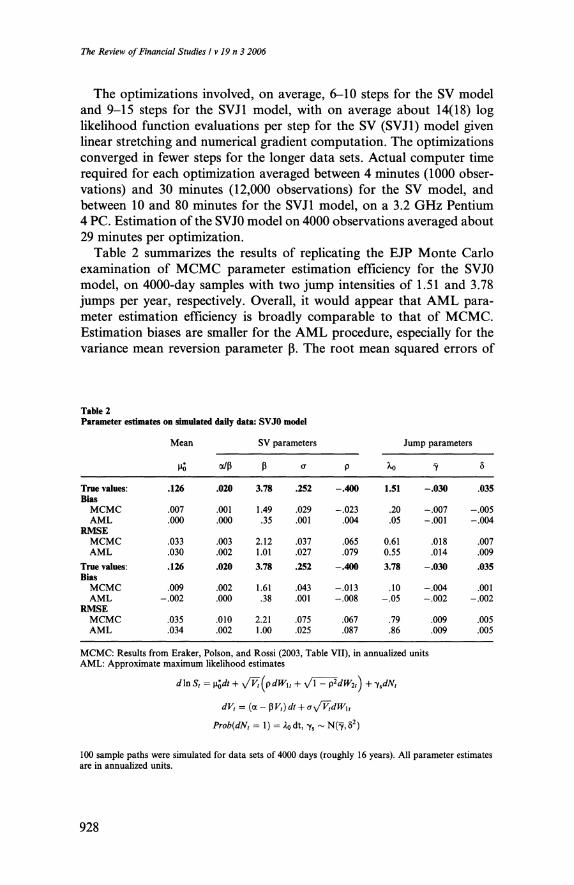
29 minutes per optimization. Table 2 summarizes the results of replicating the EJP Monte Carlo
examination of MCMC parameter estimation efficiency for the SVJ0
model, on 4000-day samples with two jump intensities of 1.51 and 3.78
jumps per year, respectively. Overall, it would appear that AML para? meter estimation efficiency is broadly comparable to that of MCMC.
Estimation biases are smaller for the AML procedure, especially for the
variance mean reversion parameter p. The root mean squared errors of
Table 2 Parameter estimates on simulated daily data: SVJ0 model
d\nSt = \i*0dt + y/Vt(pdWlt + y/1 - p2dW2t^ + ysdNt
dVt = {OL-PVt)dt + <7%/VtdWU
Prob{dNt = 1) = XQ dt, ys ~ Nft, 52)
100 sample paths were simulated for data sets of 4000 days (roughly 16 years). All parameter estimates are in annualized units.
928

Latent Affine Processes
parameter estimates are generally comparable, with neither MCMC nor
AML clearly dominating.10 Tables 3 and 4 summarize the results for the SV and SVJ1 models,
respectively. The tables also report results for parameters (a, P, a) esti?
mated by direct maximum likelihood conditional upon observing the
{Vt}]~Q sample path, using the noncentral %2 transition densities and
initial gamma distribution. These latter estimates provide an unattainable
bound on asymptotic parameter estimation efficiency for those parameters,
given that latent variance is not in fact directly observed.
The AML estimation methodology appears broadly consistent, with
the RMSE of parameter estimates roughly declining at rate l/y/T.
Table 3 Parameter estimates on simulated daily data: SV model
Returns-based estimates
dStISt = (Mo + Ui Vt)dt + y/Vt(pdWu + Vl - pW2r)
dVt = (a - PK,) dt + ay/VtdWu
100 sample paths were simulated for data sets of 1,000-12,000 days (roughly 4-48 years).
The results in EJP's Table VII were converted into annualized units. In addition, it seems likely that EJP are reporting standard deviations rather than root mean squared errors of parameter estimates, since their reported RMSEs are occasionally less than the absolute bias. Consequently, the EJP numbers were also adjusted using RMSE2=SD2 + bias2. As estimated biases were generally small, only the RMSE(p) numbers were significantly affected by this adjustment.
929

The Review of Financial Studies I v 19 n 3 2006
Table 4 Parameter estimates on simulated daily data: SVJ1 model
Returns-based estimates
dSt/St = (no + u, V, - Xx Vtk)dt + y/Vt(pdWu + Vl - P2drV2t) + (f - l)dNt
dVt = (a - p K,) rff + ay/VtdWu
Prob(dN, = 1) = Xi Vtdt, % ~ ^(7,52)
100 sample paths were simulated for data sets of 1,000-12,000 days (roughly 4-48 years). aJump parameter estimates for 7 runs (out of 100) were set to the observationally identical values of zero.
The estimated bias (average bias rows) for all parameters and parameter transformations also generally decreased with longer data samples.
There do not appear to be significant biases in the estimates of jump
parameters: the sensitivity X\ of jump intensities to changes in latent
variance, or the mean and standard deviation of jumps conditional
upon jumps occurring. However, the Xi estimates are quite noisy even
with 48 years of daily data. The RMSE of 21.0 is a substantial fraction of
the true value of 93.4.
There are substantial biases for two parameter estimates: the sensitivity
fii of expected stock returns to the current level of variance and the
parameter P that determines the serial correlation and the associated
half-life ofthe variance process. The p^ bias remains even at 12000-day
930
Latent Affine Processes
(48-year) samples; the p bias is still substantial at 16-year samples but
disappears for longer samples. The latter bias reflects in magnified fash?
ion the small-sample biases for a persistent series that would exist even if
the Vt series were directly observed, as is illustrated in the second sets of P estimates conditioned upon observing Vt.n Here, of course, the values of
latent variance must be inferred from noisy returns data, which almost
double the magnitude of the bias relative to the Frdependent estimates.
The estimates of some of the parameters of the latent stochastic var?
iance process perform surprisingly well. Daily returns are very noisy
signals of daily latent variance, and yet the RMSE of returns-based
parameter estimates of >/oc/P and P is typically less than double that of
estimates conditioned on actually observing the underlying variance.
Furthermore, the parameter estimates are highly correlated with the
estimates conditional on directly observing Vt data.
An interesting exception is the volatility of variance estimator & . Were Vt
observed, its volatility parameter ct would be pinned down quite precisely even for relatively small data sets: a RMSE of .005-.007 on data sets of
1000 observations. By contrast, when Vt must be inferred from noisy stock
returns, the imprecision ofthe Vt\t estimates increases the RMSE ofthe ct
estimate tenfold. Similar results are reported for the discrete-time log variance process in Appendix B. The mean reversion parameter estimate
for latent log variance has two to three times the RMSE of estimates
conditioned on actually observing log variance, while the RMSE of the
estimate of the volatility of log variance rises seven- to eightfold.
2.2 Filtration
A major advantage ofthe filtration algorithm is that it provides estimates
of latent variable realizations conditional upon past data. Figure 1
illustrates how volatility assessments are updated conditional upon the
last observation for three models estimated below: the stochastic volatility model (SV), the stochastic volatility/jump model with constant
jump intensities (SVJO), and the stochastic volatility/jump model with
variance-dependent jump intensities (SVJ1). For comparability with
Hentschel's (1995) study of GARCH models, the figure illustrates volati?
lity revisions (Et+\ -
Et)y/Vt+\, using the conditional moments12 of Vt+\ and the Taylor approximation
11 See Nankervis and Savin (1988) and Stambaugh (1999) for a discussion of these biases. 12 The mean and variance of Vta^t can be derived from those of Kf/r(/?tViand?2v,, respectively) by using
Equation (A.2). The mean and variance of Fr+i|r+i are updated from (k(, vt) conditional on the observed asset return by using the algorithm in Equations (13)?(17).
931

The Review of Financial Studies I v 19 n 3 2006
C o
> ? Q CO
Asset return, in standard deviations
Figure 1 News impact curves for various models The graph shows the revision in estimated annualized standard deviation (Et+\ upon observing a standardized return of magnitude yt+\/JVt\t/252.
Et)y/Vt+i, conditional
E[y/V\ ? y/E[V] ]_Var\V] 8 E[V}2
(26)
The estimates were calibrated from a median volatility day with a prior
volatility estimate of 11.4%, and initial filtered gamma distribution para? meters (?? v,) = (.00229, 5.89).
All news impact curves are tilted, with negative returns having a larger
impact on volatility assessments than positive returns. All models process the information in small asset returns similarly. The most striking result,
however, is that taking jumps into account implies that volatility updating becomes a nonmonotonic function of the magnitude of asset returns.
Under the SVJO model, large moves indicate a jump has occurred, which totally obscures any information in returns regarding latent vola?
tility for moves in excess of seven standard deviations. Under the SVJ1
model, the large-move implication that a jump has occurred still contains
some information regarding volatility, given jump intensities are propor? tional to latent variance. Neither case, however, resembles the U- and
V-shaped GARCH news impact curves estimated by Hentschel (1995).
Figure 2 illustrates the accuracy of the volatility filtration Et\/Vt con?
ditional upon using the true parameters, for the first 1000 observations
(four years) of a 100,000-observation sample generated from the SVJ1
model. The filtered estimate tracks latent volatility quite well, with an
overall R2 of 70% over the full sample. Changes in filtered volatility
932

Latent Affine Processes
0 250 500 750 1000
Figure 2 Annualized latent volatility, and its filtered estimate and standard deviation: SVJ1 model
perforce lag behind changes in the true volatility, since the filtered esti?
mate must be inferred from past returns. The absolute divergence was
usually less than 5% (roughly two standard deviations) but was occasion-
ally larger. To put this error in perspective, the volatility estimate in mid-
sample of 15% when the true volatility was 10% represents a substantial
error when pricing short-maturity options. The magnitude of this error
reflects the low informational content of daily returns for estimating latent volatility and variance.
2.2.1 Filtration diagnostics. A key issue is whether force-fitting poster- ior distributions into a gamma distribution each period reduces the
quality of the filtrations. Two sets of diagnostics were used on simulated
data. First, the accuracy and informational efficiency of the variance
filtration was compared with various GARCH approaches and with
Gallant and Tauchen's (2002) reprojection technique. Second, the extent
of specification error in conditional distributions was assessed using
higher-moment and quantile diagnostics. The diagnostics were run on
two 200,000-day (794-year) data sets simulated from the SV and SVJ1
processes, respectively. The first 100,000 days were used for in-sample estimation and testing, while the subsequent 100,000 days were used for
out-of-sample tests.
Three GARCH models were estimated on the SV simulated data: the
standard GARCH(1,1) and EGARCH specifications and Hentschel's
933

The Review of Financial Studies I v 19 n 3 2006
(1995) generalization (labeled HGARCH) that nests these and other
ARCH specifications. Filtration performance was assessed based on
how well the filtered volatility and variance estimates tracked the true
latent values, as measured by overall R2.
As shown in Table 5, the approximate maximum likelihood SV filtra?
tion outperforms all three ARCH models, when either the true SV para? meters or the parameters estimated from the full sample are used.
However, the EGARCH and HGARCH specifications that take into
account the correlations between asset returns and volatility shocks per? form almost as well as the SV model when estimating latent volatility and
variance from past returns.
For the SVJ1 data with jumps, the ARCH models were modified to t-
ARCH specifications to capture the conditionally fat-tailed property of
returns. Despite the modification, the f-GARCH and f-EGARCH filtra-
tions performed abysmally, while even the r-HGARCH specification sub?
stantially underperformed the SVJ1 filtration The problem is, of course, the
jumps. As illustrated in Figure 1, the optimal filtration under the postu- lated stochastic volatility/jump process is essentially to ignore large outliers.
The GARCH failure to do this can generate extremely high volatility estimates severely at odds with true latent volatility. For instance, the
simulated data happened to include a crash-like -21% return. The (in-
sample) annualized volatility estimates of 108%, 159%, and 32% from the
f-GARCH, f-EGARCH and /-HGARCH models for the day immediately after the outlier greatly exceeded the true value of 10%.
Table 5 Volatility and variance filtration performance under various approaches
Two samples of 200,000 daily observations (794 years) were generated from the SV and SVJ1 processes, respectively. In-sample fits use the first 100,000 observations for parameter estimation and filtration. Out- of-sample fits use the subsequent 100,000 observations for filtration.
934

Latent Affine Processes
The informational efficiency of the algorithm's filtrations was assessed
using a reprojection technique based on that in Gallant and Tauchen
(2002). The true variance Vt was regressed on current and lagged values of
the filtered variance estimates Vt\t, as well as on lags of returns and
absolute returns and a constant. 3 Comparing the resulting R2s with
those of the AML algorithm tests jointly for forecasting biases and for
any information not picked up by the contemporaneous filtered
estimate Vt\t}A The lag length was set equal to 4.32 ln 2/p (4.32 half-
lives of variance shocks), which implies from Equation (22) that less than
5% of the potential information in the omitted data from longer lags is
still relevant for variance forecasting. Given p estimates, this generated 128- and 178-day lag lengths ofthe three dependent variables for the SV
and SVJ1 models respectively. All regressions were run in RATS.
The reprojection results in Table 5 indicate very little information is
picked up by the additional regressors. In-sample, the R2s ofthe variance
estimates increase only from 69.0% to 69.5% for the SV variances generated from the SV process, and from 70.0% to 70.6% for the SVJ1 variances. In
the out-of-sample tests, there is virtually no improvement in forecasting
ability. The in-sample increase in R2 are of course statistically significant,
given almost 100,000 observations. Nevertheless, the virtually identical R2
performance suggests little deterioration in latent variance estimation from
approximating prior distributions by an gamma distribution.
2.2.2 Diagnostics of conditional distributions. Two additional diagnos- tics were used to assess how well gamma approximations captured the
overall conditional distributions of latent variance. The first diagnostic was based upon computing higher conditional moments of posterior distributions. The algorithm uses only the posterior mean and variance
of the latent variable as inputs to next period's prior distribution. How?
ever, the posterior skewness and excess kurtosis can be computed by similar numerical integration methods and compared with the gamma- based values ofl/y/vt+\ and 6/v,+i, respectively.
The results reported in Table 6 indicate the posterior distributions of
latent variance from the SV model are invariably positively skewed and
leptokurtic. The divergences in moments from the gamma moments are
positive but near zero on average, and with a small standard deviation.
Overall, it would appear that the gamma posterior approximation gener?
ally does a good job. However, the min/max ranges for moment
13 Gallant and Tauchen (2002) use lagged variance estimates from their SNP-GARCH approach as regressors.
14 Testing the improvement in R2 via an F-test is statistically equivalent to examining whether the regressors have any explanatory power for the residuals Vt ? Vt\t-
935

The Review of Financial Studies I v 19 n 3 2006
Table 6 Higher Conditional Moments of Latent Variance
Summary statistics of the conditional moment estimates, and of the divergence from gamma-based estimates, based on 100,000 observations of simulated data from the SV and SVJ1 models, respectively.
divergences indicate there are specific days on which a more flexible speci? fication might be preferable.
The posterior moments for the SVJ1 model are also generally close to
the gamma moments. Again, however, there are specific days in which a
more flexible specification is desirable. In particular, the posterior dis?
tribution can occasionally be negatively skewed and platykurtic. This
reflects the fact that the posterior distributions for latent variance from
the SVJ1 model are mixtures of distributions, the posterior distributions
conditional upon n jumps occurring weighted by the posterior probabil? ities of ?jumps. For days with substantially ambiguity ex post regarding whether a jump has or has not occurred, the posterior distribution for
latent variance can be multimodal and platykurtic. It should be emphasized that all of the above posterior moment com-
putations involve updating conditional upon a gamma prior distribution.
As such, they provide a strictly local diagnostic of whether a more flexible
class of distributional approximations would better capture posterior distributions at any single point in time.
A second diagnostic was used to assess the overall performance of the
approximate conditional distributions: the frequency with which simulated
Vt realizations fell within the quantiles of the conditional Vt\t gamma distributions. The realized frequencies over runs of 100,000 observations
indicate the gamma conditional distributions do, on average, capture the
conditional distribution of Vt realizations quite accurately:
Quantile/?: .010 .050 .100 .250 .500 .750 .900 .950 .990
SV SVJ1
936

Latent Affine Processes
The above results were for filtrations using the true parameter vector 9.
The results using in-sample estimated 8 were identical.
In summary, the approximate maximum likelihood methodology per? forms well on simulated data. Parameter estimation is about as efficient
as the MCMC approach for two processes for which we have bench-
marks: the discrete-time log variance process, and the continuous time
stochastic volatility/jump process SVJO. Volatility and variance filtrations
are more accurate than GARCH approaches, especially for processes with jumps, while the filtration error is virtually unpredictable by
EMM-style reprojection. Finally, the mean- and variance-matching
gamma conditional distributions assess the quantiles of variance realiza?
tions quite well on average. However, there are individual days for which
matching higher moments better would be desirable.
3. Estimates from Stock Index Returns
For estimates on observed stock returns, I use the 11,076 daily S&P 500
returns over 1953 through 1996 that formed the basis for Andersen,
Benzoni, and Lund's (2002) EMM/SNP estimates. I will not repeat the
data description in that article, but two comments are in order. First, Andersen et al. prefilter the data to remove an MA(1) component that
may be attributable to nonsynchronous trading in the underlying stocks.
Second, there were three substantial negative outliers: the -22% stock
market crash of October 19, 1987, the 7% drop on September 26, 1955, that followed reports of President Eisenhower's heart attack, and the 6%
minicrash on October 13, 1989.
The first three columns of Table 7 present estimates of the stochastic
volatility model without jumps (SV) from Chernov et al., Andersen et
al., and the AML methodology of this article.15 As discussed in CGGT,
estimating the parsimonious stochastic volatility model without jumps creates conflicting demands for the volatility mean reversion parameter
P and the volatility of volatility parameter o\ Extreme outliers such as
the 1987 crash can be explained by highly volatile volatility that mean-
reverts within days, whereas standard volatility persistence suggests lower volatility of volatility and slower mean reversion. In CGGT's
estimates, the former effect dominates; in ABL's estimates, the latter
dominates.
AML estimates are affected by both phenomena, but matching the
volatility persistence clearly dominates. While constraining a to the
CGGT estimate of 1.024 substantially raises the likelihood of the outliers
in 1955,1987, and 1989, this is more than offset by likelihood reductions for
the remainder of the data. The overall log likelihood fails from 39,234 to
' The ABL estimates are from their Table IV, converted to an annualized basis.
937
The Review of Financial Studies I v 19 n 3 2006
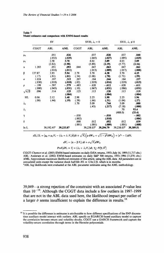
Table 7 Model estimates and comparison with EMM-based results
dS,/St = [mo + u, V, - (Ao + A, Vt)k]dt + y/Vt(pdWu + >/l - pW*) + (e7* - \)dNt
dVt = (a - p F,) A + (Ty/VtdWu
Prob[dNt = 1] = (Ao + A, K,)A, V^[7,52] CGGT: Chernov et al. (2003) EMM-based estimates on daily DJIA returns, 1953-July 16,1999 (11,717 obs.) ABL: Andersen et al. (2002) EMM-based estimates on daily S&P 500 returns, 1953-1996 (11,076 obs.) AML: Approximate maximum likelihood estimates of this article, using the ABL data All parameters are in annualized units except the variance shock half-life HL = 121n2/p, which is in months. aABL log likelihoods were evaluated at the ABL parameter estimates using the AML methodology.
39,049?a strong rejection ofthe constraint with an associated P- value less
than 10~16. Although the CGGT data include a few outliers in 1997-1999
that are not in the ABL data used here, the likelihood impact per outlier of
a larger a seems insufficient to explain the difference in results.16
16 It is possible the difference in estimates is attributable to how different specifications ofthe SNP discrete- time auxiliary model interact with outliers. ABL specify an EGARCH-based auxiliary model to capture the correlation between return and volatility shocks. CGGT use a GARCH framework and capture the volatility-return correlation through terms in the Hermite polynomials.
938

Latent Affine Processes
Although the AML stochastic volatility parameter estimates are
qualitatively similar to those of ABL on the same data set, there are
statistically significant differences. In particular, I estimate a higher
volatility of volatility (.315 instead of .197) and faster volatility mean
reversion (half-life of 1.4 months, instead of 2.1 months). The former
divergence is especially significant statistically, given a standard error
of only .018.17 The estimate ofthe average annualized level of variance
is also higher: (.125)2, rather than (.112)2. The estimates ofthe correla?
tion between volatility and return shocks are comparable. The substan?
tial reduction in log likelihood of the six ABL parameter estimates is
strongly significant statistically, with a P-value of 10~15. It appears that
the two-stage SNP/EMM methodology used by Andersen et al. gener- ates a objective function for parameter estimation that is substantially different from my approximate maximum likelihood methodology.
As found in the earlier studies, adding a jump component substan?
tially improves the overall fit. As indicated in the middle three columns
of Table 7,1 estimate a more substantial, less frequent jump component than previous studies: three jumps every four years, of average size
-1.0% and standard deviation 5.2%. As outliers are now primarily
explained by the jump component, the parameters governing volatility
dynamics are modified: a drops, and the half-life of volatility shocks
lengthens. The divergence of parameter estimates from the ABL esti?
mates is again strongly significant statistically. Bates (2000) shows that a volatility-dependent jump intensity com?
ponent X\Vt helps explain the cross section of stock index option
prices. Some weak time series evidence for the specification is provided in Bates and Craine (1999), while Eraker et al. (2003) find stronger
empirical support. In contrast to the results in ABL, the final column
of Table 7 indicates that jumps are indeed more likely when volatility is
high. The hypothesis that Ai=0 is rejected at a P-value of 5 x 10~8 . The
time-invariant jump component X0 ceases to be statistically significant when X-i is added. The Monte Carlo simulations in Table 4 establish
that the standard error estimates are reasonable, and that the AML
estimation methodology can identify the presence of time-varying
jump intensities.
Standard maximum likelihood diagnostics dating back to Pearson
(1933) can be used to assess model specification. As in Bates (2000), I
use the normalized transition density
yll=N-l[CDF(y^l\YhQ)} (27)
17 The Monte Carlo RMSE results in Tables 2 and 3 for 12,000-observation data samples indicate that the estimated asymptotic standard errors in Table 7 are reliable in general.
939
The Review of Financial Studies I v 19 n 3 2006
where 7V-1 is the inverse ofthe cumulative normal distribution function, and the cumulative distribution function CDF is evaluated from the
conditional characteristic function by Fourier inversion given parameter estimates 0. Under correct specification, the y*s should be independent and identical draws from a normal JV(0, 1) distribution.
Figure 3 examines specification accuracy using normal probability
plots generated by Matlab, which plot the theoretical quantiles (line) and empirical quantiles (+) against the ordered normalized data v*.
Unsurprisingly, the stochastic volatility model (SV) is unable to match
the tail properties of the data; there are far too many extreme outliers.
The models with jumps (SVJO, SVJ1) do substantially better. However, both have problems with the 1987 crash, which is equivalent in probabil?
ity to a negative draw of more than five standard deviations from a
Gaussian distribution. As such moves should be observed only once
every 14,000 years, the single 1987 outlier constitutes substantial evidence
against both models.
To address this issue, an additional stochastic volatility/jump model
SVJ2 was estimated with two separate jump processes, each with Vt-
dependent jump intensity.18 The resulting estimates for the stochastic
volatility component are roughly unchanged; the jump parameters become
Prob[dNu = 1] = 131.1 Vtdt, ln(l +k\) -#[.001, (.029)2]
Prob [dN2t = 1] = 2AVtdt, ln(l + k2) -#[-.222, (.007)*]. 2l (28)
The conditional distribution of daily returns is approximately a mixture
of three normals: diffusion-based daily volatility that varies stochasti-
cally over a range of .2%?1.8%, infrequent symmetric jumps with a
larger standard deviation of 2.9% and a time-varying arrival rate that
averages 1.85 jumps per year, and an extremely infrequent crash corre?
sponding to the 1987 outlier. Log likelihood rises from 39,309.51 to
39,317.81?an improvement almost entirely attributable to a better fit
for the 1987 crash. The increase in log likelihood has a marginal sig? nificance level of .0008 under a likelihood ratio test, given three addi?
tional parameters. The j*-score for the 1987 crash drops in magnitude to a more plausible
value of -3.50. As shown in Figure 3, the resulting empirical and theore?
tical quantiles for the SVJ2 model are much more closely aligned. How?
ever, there remain small deviations from perfect alignment that indicate
some scope for further model improvement.
Multiple-jump processes are equivalent to a single-jump process in which the jump is drawn from ; mixture of distributions.
940

Latent Affine Processes
:s
I
U
s +
i
?8.
9s O
??
fi-S S 1-1
H
'II En Z H
941

The Review of Financial Studies I v 19 n 3 2006
3.1 Filtration
Figure 4 shows the filtered estimates ofthe latent state variable \[Vt from
the SVJ1 model, and the divergence between SVJ1 and SV estimates of
diffusive volatility y/Vt. Those estimates are generally almost identical,
except following large positive or negative stock returns. For instance, the 1955 and 1987 crashes have much more of an impact on volatility assessments under the SV model than under the jump models?as one
would expect from the news impact curves in Figure 1.
The number of jumps on any given day is also a latent variable that can
be inferred from observed returns. It is shown in Appendix A that the
joint conditional distribution of log-differenced asset prices and the num?
ber of jumps AiV,+i = Nt+\ ? Nt has an affine specification. Conse?
quently, the characteristic function GAN(il,\Yt+i) =
E[e^Nt^\yt+x, Yt] can be evaluated by Proposition 1.
While it is possible to evaluate the daily probability that n jumps occurred by Fourier inversion of Gajv, it is simpler to estimate the
number of jumps: E[ANt+\\Yt+\] = G^N(0\Yt+\). At the daily horizon,
ANt+i is essentially binomial, and the estimated number of jumps is
approximately the probability that a jump occurred. Unsurprisingly, in
Figure 5 large moves are attributed to jumps, and small moves are not.
Intermediate moves of roughly three to five times the estimated latent
standard deviation imply a small probability that a jump occurred. It is
the accumulation of these small jump probabilities for the moderately
~i-1-1-1-1-r
53 58 63 68 73 78 83 88 93
Figure 4 Annualized filtered volatility estimate Ety/Vt from the stochastic volatility/jump model SVJ1, and its divergence from SV volatility estimates.
942

Latent Affine Processes
A3r 871019
891013
550926
-G8-
M-
?M-
-M- t*
-16 ?12 -8 -4 0 4 8
Figure 5 /_- Estimated number of jumps, versus standardized returns yt+\/Jvt\t/252, SVJO model The values are approximately the probability for each day that a jump occurred.
frequent intermediate-sized moves that underpin the overall estimate of
jump intensities (e.g., .744 jumps per year in the SVJO model).
4. Implications for Option Prices
One ofthe major advantages of using affine processes is their convenience
for pricing options. If the log ofthe pricing kernel is also affine in the state
variables, the "risk-neutral" asset price process used when pricing options is also affine, and options can be rapidly priced by Fourier inversion of
the associated exponentially affine characteristic function. Under the risk-
neutral parameters 0*, the upper tail probability conditional upon know?
ing latent variance Vt is
P2 = Prob* [ln(St+T/St) > ln(X/St) | Vt)
5 exp[C*(i*,0;r) + Z>*(/O,0;T) Vt - min{X/St)]
~2 +
2ir]_c m dQ>
(29)
where C*(*) and ?>*(?) are variants of C(*) and /)(?) evaluated at the risk-
neutral parameters 9* and time interval T. The value for a European call
option c(St, Vt, T; X) with maturity Tand strike price Xcan be evaluated
by using dc/dX=-e~rTP2, substituting Equation (29) for P2, and inte-
grating with respect to X:
943

The Review of Financial Studies I v 19 n 3 2006
c(Sh Vu T\ X) = Ste~d<T
"1 1 f^ eC*(i?AT)+D*(i?,0;T)Vt-mn(X/St) ^"| (30)
2 2'kJ_oq e~rTX
i*(1-i?)
where dt is the current dividend yield, and the ex-dividend spot price Ste~dtT is a constant of integration determined by the value of a call
option with zero strike price.19 Given the affine structure inside the
integrand in Equation (30), an econometrician's valuation of a European call option conditional upon observing past returns Yt and the current
asset price St is
c(Sh T; X\Yt) = E[c(Sh Vu T- X)\YU St] = Ste -dtT
e~rT) 1 ]_
r?? ec*^ T)Gt^D*^ 0; T^e-mn{x/st)
-
2 +
W-oo i*(1-M>) (31)
The filtration used in estimating the conditional characteristic function
G>l,(*) of current latent variance is based on the objective parameter values, not the risk-neutral parameters. The option valuation in Equation
(31) is roughly equivalent to using a filtered variance estimate Vt\t in (30) and adding a Jensen's inequality correction for state uncertainty Pt\t.
The risk adjustments incorporated into the divergence between the
actual parameters 9 and the risk-neutral parameters 0* depend upon the
pricing kernel Mt. The general affine pricing kernel specification com?
monly used in the affine literature takes the form
d\nMt = \imdt -Rd\nSt- RvdVt - RjysdNt, (32)
where \im is such that Et(dMt/Mt) = -rtdt. This reduced-form specifica? tion nests various approaches. For instance, the submodel with
Rv = Rj = 0 is the myopic power utility pricing kernel used in the
implicit pricing kernel literature and in Coval and Shumway's (2001)
empirical examination of the profits from straddle positions. If St is
viewed as a good proxy for overall wealth, R measures relative risk
aversion. More generally, R reflects the projection of pricing kernel
innovations upon asset returns and can be greater or less than the coeffi?
cient of relative risk aversion.
Rv determines a volatility risk premium in addition to the wealth-
related effect that volatility innovations tend to move inversely with
19 This approach is equivalent to but more efficient than the approaches in Bates (1996, 2000) and Bakshi and Madan (2000). Those approaches require two univariate integrations, whereas Equation (30) has only one, with an integrand that falls off more rapidly in O. Carr and Madan (2000), Lewis (2001), and Attari (2004) have derived similar formulas by alternate methods.
944
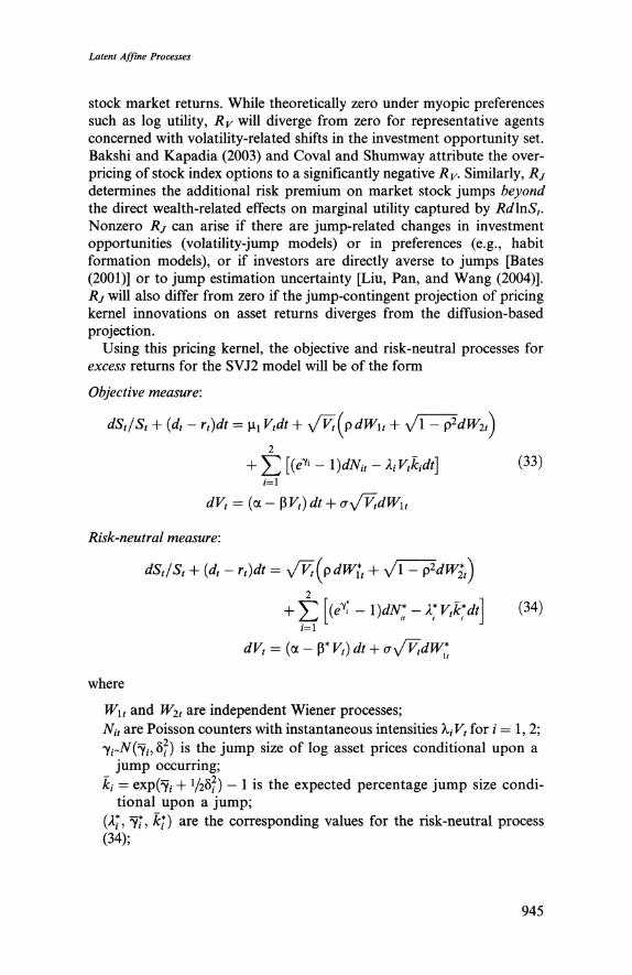
Latent Affine Processes
stock market returns. While theoretically zero under myopic preferences such as log utility, Rv will diverge from zero for representative agents concerned with volatility-related shifts in the investment opportunity set.
Bakshi and Kapadia (2003) and Coval and Shumway attribute the over-
pricing of stock index options to a significantly negative Rv. Similarly, Rj determines the additional risk premium on market stock jumps beyond the direct wealth-related effects on marginal utility captured by RdlnSt. Nonzero Rj can arise if there are jump-related changes in investment
opportunities (volatility-jump models) or in preferences (e.g., habit
formation models), or if investors are directly averse to jumps [Bates
(2001)] or to jump estimation uncertainty [Liu, Pan, and Wang (2004)].
Rj will also differ from zero if the jump-contingent projection of pricing kernel innovations on asset returns diverges from the diffusion-based
projection.
Using this pricing kernel, the objective and risk-neutral processes for
excess returns for the SVJ2 model will be of the form
Objective measure:
dSt/St + (dt -
rt)dt = ]ix Vtdt + y/Vt(pdWu
+ y/\ - P2dW2t^j
2
+ YI K*7i -l ^dNtt -ki v&idt\ (33) i=i
dVt = (a -
PK,) dt + ay/VtdWxt
Risk-neutral measure'.
dSt/St + {dt - rt)dt = y/Vt(pdw;t
+ y/\ - P*dw?)
2 V 1 + 5Z (** ~
x^dNl" KvKdt\ (34)
i=\
dVt = (a - P* Vt) dt -f ay/VtdWl
where
Wu and W2t are independent Wiener processes;
Nit are Poisson counters with instantaneous intensities XtVt for / = 1,2;
li~N(yi, 8?) is the jump size of log asset prices conditional upon a
jump occurring;
kf = exp(7; + V^S?) - 1 is the expected percentage jump size condi?
tional upon a jump;
(A*, 7*, k*) are the corresponding values for the risk-neutral process
(34);
945

The Review of Financial Studies I v 19 n 3 2006
W*t and N*t are the corresponding risk-neutral Wiener processes and
Poisson counters.
If dividend yields and interest rates are nonstochastic, Equation (34) is
also the risk-neutral process for futures returns used in pricing futures
options. The affine pricing kernel constrains both objective and risk-neutral
parameter values. As discussed in Bates (1991, Appendix 1), the instanta-
neous equity premium estimated under the objective probability measure is
(Mo + V>iVt + dt- rt)dt = -Et dSt\fdMt\
St)\Mt) (35)
For the SVJ2 model, this implies
Mo=0 2
ii! = R + Rvpo + Y^ (Kkl ~ Wi)
i=i
while the risk-neutral parameter values used in pricing derivatives are
^=^[1+^1^ = 1
= kt exp[-(tf + Rj)yt + i/2(R + Rj)252}
7* = y. + Cov(yt) dln Mt\dNt = 1
= yi-(R + RJ)82
\dVtdMt
(36)
(37)
P* = P"? Vt Mt
= fi + Rpcr + Rvo2.
4.1 Estimated option prices To illustrate the option pricing implications ofthe AML estimation methodol?
ogy, I will focus upon the myopic power utility pricing kernel, with
Rv = Rj = 0. This is done for two reasons. First, the appropriate risk
adjustments for pricing options can be estimated solely from past stock
index excess returns under the AML methodology presented above, whereas
pricing volatility or jump risk premia under other specifications requires
incorporating additional information from option prices or option returns.
Second, the power utility pricing kernel is a useful performance mea?
sure that has been previously employed for assessing returns on options
946

Latent Affine Processes
[Coval and Shumway (2001)] and on mutual funds [e.g., Cumby and Glen
(1990)]. It is also the standard benchmark against which implicit pricing kernels are compared [Rosenberg and Engle (2002) and Bliss and Pana-
girtzoglou (2004)]. While equivalent to a conditional CAPM criterion
when stock market and option returns are approximately conditionally normal, using a power utility pricing kernel is more robust to the sub?
stantial departures from normality observed with returns on out-of-the-
money options.20 Large deviations of observed option prices from the
power utility valuations indicate investment opportunities with an exces-
sively favorable conditional return/risk tradeoff. Of course, it is possible that such investment opportunities can be rationally explained by inves?
tors' aversions to time-varying volatility or to jump risk, which would
show up in nonzero Rv or Rj. Since Equation (33) requires excess returns, the ABL data were
adjusted by monthly dividend yields and 1-month Treasury bill rates
obtained from the Web sites of Robert Shiller and Ken French, respec?
tively. In addition, the ABL data set was extended through 2001 using CRSP data, for use in out-of-sample tests. Since the substantial autocor-
relations in daily S&P 500 index returns estimated by Andersen et al.
(2002) over 1953-1996 were not apparent over the post-1996 period, post- 1996 excess returns were used directly, without prefiltration.
Table 8 contains estimates of the SVJ2 model on returns and excess
returns and the corresponding estimates of the risk-neutral parameters under the myopic power utility pricing kernel. Unsurprising, the uncon-
strained SVJ2 estimates on raw and excess returns in the first two rows of
each panel are virtually identical, except for a difference in the mean
parameter |ii. The dividend and interest rate series are smooth, inducing little change in the estimates of volatility dynamics and jump risk.
Affine pricing kernel models imply that [i0 = 0 for the SVJ2 model. The
estimated sensitivity |ii of the equity premium to the current level of
variance determines the risk aversion parameter R for the power utility
pricing kernel and constrains the risk aversion parameters for other
models. In Table 8, the |i0 = 0 constraint is borderline insignificant, with a marginal significance level of 6.8% under a likelihood ratio test.
The risk aversion estimate is approximately 4. The implications for the
risk-neutral parameters used in option pricing are twofold. First, the risk-
neutral frequency of 1987-like crashes is more than double that of the
objective frequency. Second, the risk-neutral volatility dynamics implicit in the term structure of implied volatilities involve somewhat slower
mean reversion to a somewhat higher level: a half-life of 2.0 months
Goetzmann, Ingersoll, Spiegel, and Welch (2002) discuss problems with the traditional Sharpe ratio performance measure when funds can take positions in options.
947

The Review of Financial Studies I v 19 n 3 2006
Table 8 Estimates of the multi-jump model SVJ2 and associated risk-neutral parameter estimates
Data: daily S&P 500 returns and excess returns over 1953-1996. Standard errors are in parentheses.
rather than 1.8 months, and a long-run level of (12.8%)2 instead of
(11.9%)2. For comparison, daily settlement prices for the Chicago Mercantile
Exchange's American options on S&P 500 futures and the underlying futures contracts were obtained from the Institute for Financial Markets
for the period from the option contracts' inception on January 28, 1983,
through June 29, 2001. The use of end-of-day option prices synchronizes
nicely with the AML variance filtration, which uses closing S&P 500
index returns. The shortest-maturity out-of-the-money call and put
options with a maturity of at least 14 days were selected. The correspond?
ing implicit standard deviations (ISDs) were computed using the Barone-
Adesi and Whaley (1987) American option pricing formula, for compar? ison with those computed from AML European option price estimates. In
addition, a benchmark at-the-money ISD was constructed for each day
by interpolation.21
Figure 6 shows the observed and estimated volatility smirks for out-of-
the-money put and call options on December 31, 1996, which was the last
day of the ABL data set. Several results are evident. First, the ISDs
21 A minor issue is the difference between American and European options, and the computation of associated ISDs. The price of an American futures option is bounded below by the European price and bounded above by the future value ofthe European price. The resulting error in annualized European at- the-money ISD estimates is bounded by ?lSDt x rT{ ? 0.04% on December 31, 1996), while the errors for out-of-the-money ISD estimates are even smaller.
948

Latent Affine Processes
-15%
Figure 6 Observed and estimated ISDs for 17-day Jan.1997 S&P 500 futures options on Dec.31,1996 The dark grey area is the 95% confidence interval given only parameter estimation uncertainty. The light grey area is the 95% confidence interval given both parameter and state uncertainty.
estimated from stock index returns exhibit a substantial volatility smirk.
This smirk partly reflects the negative correlation between asset returns
and volatility shocks but also reflects the substantial and time-varying crash risk?in particular, the risk-adjusted estimate of infrequent 1987-
like crashes.
Second, estimates are imprecise. Option price estimates and the asso?
ciated ISDs contain two types of error:
9c Tr ,-. dc parameter estimation error, with variance ?7 Var(Q) ?, and
c/0 a9
filtration error (or state uncertainty), with variance '_dcj
KdvAt/ iV
The at-the-money estimated ISD contains little parameter uncertainty,
reflecting the relative robustness of volatility estimates to model specifica? tion. However, there is considerable state uncertainty regarding the cur?
rent level of Vt and the at-the-money ISD. This state uncertainty reflects
the relatively low informational content of daily returns and could be
reduced by using more informative data sources. Out-of-the-money put
949

The Review of Financial Studies I v 19 n 3 2006
and call option prices are less affected by state uncertainty but are more
affected by parameter uncertainty. This reflects the difficulties in estimat?
ing the jump parameters, which are of key importance in determining the
probability of these options paying off.
Third, the deviations between estimated and observed ISDs were some?
times large enough to be statistically significant. S&P 500 futures options were mostly overpriced on December 31, 1996, from the perspective ofa
myopic power utility investor with a risk aversion of 4 who is 100%
invested in S&P 500 stocks. This sort of overpricing is responsible for
the high Sharpe ratios reported by various authors for option-selling
strategies.
Figure 7 shows at-the-money ISDs for short-maturity options on Wednes-
days over 1983-2001, the corresponding AML filtered ISD estimates, and
the divergence between the two. The estimates prior to 1997 are "in-sample," in that the parameter estimates underlying the filtration are from the full
1953-1996 data set. The post-1996 filtered estimates are out-of-sample. Overall, the filtered estimates track the at-the-money option ISDs
reasonably well. There are, however, some interesting and persistent
50%
40%
30%
20%
10%
0 ISD options- I& ts (right scale)
10%
0
-10%
opnons /o ^ ?-' " i
H-1-1-\- H-1-1-1-h 83 84 85 86 87 88 89 90 91 92 93 94 95 96 97 98 99 00 01
Figure 7 Observed and estimated ISD's for at-the-money S&P 500 futures options; Wednesday data Estimated ISD's are based on SVJ2 parameter estimates from 1953-1996, and on filtered variance estimates from daily returns. The grey area is the 95% confidence interval given both parameter and state uncertainty.
950

Latent Affine Processes
deviations between the two series. For instance, at-the-money options were substantially overpriced during the two years preceding the 1987
crash, when judged against the time series estimates of appropriate risk-
adjusted value. The extent of the overpricing soared after the crash but
gradually dwindled over 1988-1991, only to reemerge in late 1996 and in
subsequent years. The mispricing was especially pronounced following the minicrash of October 1997, and in the fall of 1998. Overall, option
overpricing was most pronounced when observed and estimated ISDs
were both relatively high?a result mirroring standard results from
regressing realized volatility on ISDs.
Over 1988-1996, ISDs averaged 2.2% higher than the time series valua-
tions, while the average gap was 4.6% over 1997-2001. It is possible that
this greater gap reflects out-of-sample instabilities in the time series
model. However, it seems more plausible to attribute it to structural shifts
in the stock index options market?in particular, to the bankruptcy of
Long Term Capital Management in August 1998. By 2000, estimated
ISDs were again tracking observed ISDs fairly closely.
5. Conclusions and Extensions
This article has presented a new approximate maximum likelihood
methodology for estimating continuous-time affine processes on dis?
crete-time data: both parameter values and latent variable realizations.
Results on simulated data indicate the parameter estimation efficiency is
excellent for those processes for which we have performance bench-
marks. Furthermore, the approach directly generates a filtration algo? rithm for estimating latent variable realizations, of value for risk
management and derivatives pricing. Most other approaches must
append an additional filtration procedure to the parameter estimation
methodology. The AML approach was used to estimate the parameters of an affine
stochastic volatility/jump process, using the data set of Andersen,
Benzoni, and Lund (2002). Parameter estimates were similar to the
EMM-based estimates of Andersen et al., but differ in statistically sig? nificant fashions. In particular, I find a generally higher volatility of
volatility, a more substantial jump component, and strong support for
the hypothesis that jumps are more likely when volatility is high. Further?
more, Monte Carlo simulations establish that the AML estimation meth?
odology can reliably identify these phenomena. The AML methodology differs substantially from the SNP/EMM
methodology used by Andersen et al., so the source of divergence is not
immediately apparent. It does appear that the EMM methodology may be sensitive to precisely how the auxiliary discrete-time SNP model is
specified?especially in the presence of infrequent large outliers such as
951

The Review of Financial Studies I v 19 n 3 2006
the 1987 crash. Chernov et al. (2003) find very different estimates from
Andersen et al. for the stochastic volatility model, for a similar data set
but a different auxiliary model. A Monte Carlo examination of whether
the EMM estimation procedure is indeed robust to stochastic volatility/
jump processes would appear desirable.
This article has focused on classical maximum likelihood estimation.
However, the recursive likelihood evaluation methodology presented here
can equally be used in Bayesian estimation, when combined with a prior distribution on parameter values.
More recent research into volatility dynamics has focused on the addi?
tional information provided by alternate data sources, for example, high- low ranges, or "realized" intradaily variance. Furthermore, it appears from Alizadeh, Brandt, and Diebold (2002) and Andersen, Bollerslev,
Diebold, and Ebens (2001) that the additional data are sufficiently infor?
mative about latent variance that single-factor models no longer suffice.
The complexities of using alternative data sources in conjunction with
multifactor models of latent variance will be explored in future research.
Appendix A
A.l Conditional moment dynamics For fully affine stochastic processes, the conditional joint cumulant generating function is
ln F(<D, \|/| Yt) = ln ?[*?"+!+**'+' | Yt] (A'1}
= C?(0, v|/) + C'(0>, ?)*+*,!,[/>(*, +)]
where gt\t($) = lnE[e*x'\Yt] is the cumulant generating function of latent xt conditional upon using the approximate maximum likelihood filtration and observing data Yt. Condi? tional means and variances can be evaluated by taking derivatives of the joint cumulant generating function:
^/+i = CS + C^+4(0)Z)?
= C% + Ciyt+x,ltDi>
xt+i\t = Cj + C?yt + *,|r Aj, (A.2)
?t+\\t = C^j, + C^yt + g',|,Ajn|/ + g"\tDl
= tfft + C^yt + *,|/A|n|r + Pt\tD$
where all derivatives of C?, C and D are evaluated at <J> = i|/ = 0. The first and second derivatives of gt\t, evaluated at D(0,0) = 0, give the time-/ conditional mean and variance of xt.
Conditional moment dynamics can be evaluated by writing each noncentral moment as the sum of the prior expectation and the revision in expectations in light of new data. For conditional means this takes the form
(cJ=(^Mc4?)a;M:n:)
952

Latent Affine Processes
where w,+i = yt+l - Etyt+i and v,+i = x,+i|,+i - xt+i\t. Using the same approach for revising the conditional second noncentral moment of the
latent state variable yields
(P,+i|,+i + *?+i|,+i) = (Pt+\\t + *?+i|r) + (?+1 " &t)x}+l. (A.4)
Substituting in the expressions for Pt+i\t and xt+i\t from Equation (A.2) yields the dynamics of conditional variance:
Pr+i,,+i = Cj^ + Cfayt + Z)w^|, + Z^P,,, + (w,+i - n?+1), (A.5)
where w/+i = (P?+i - Et)x2t+l - 2vt+\ (Cj + Cj^ + AiAi*)- This, along with Equation (A.3), yields the vector autoregression for conditional moments that is given in Equation (22).
The dynamics of the higher noncentral conditional moments of xt+i and yt+1 can be evaluated similarly, using derivatives of the moment generating function
P(0>, x|/|Yt) = ec0(*.+)+^(*^G,? [/)(<&, x|/)] (A.6)
to evaluate Etx^+l and Etyf+l for arbitrary integer ra. The mth derivative of Gt\t, evaluated at Z>(0,0) = 0, is the noncentral conditional moment Etxf.
A.2 Joint moment generating functions from continuous-time affine
processes Let
P(0,+,$|5r, ^,AT? r, P) = P^+*Fr+^r|^ ^ ^] (A.7)
be the joint moment generating function of the future variables zt = (sr, VT, NT) condi? tional upon observing zt today, where st is the log asset price, Vt is the instantaneous variance, and Nt is a Poisson counter. Since F is a conditional expectation, it is a martingale:
P,[</P(.|s? V?Nt,t,T)]=0. (A.8)
Expanding this by the jump-diffusion generalization of Ito's lemma yields the backwards
Kolmogorov equation that F must solve for a given stochastic process. For the affine
processes in this article, the solution is exponentially affine in the state variables, and
depends on the time gap r=T ? t between observations:
P(0>,i|/,$|j? VuNt; t) = exp[<Ds, + %Nt + C(G>,x|/,$;r) + Z)(<D,x|/,$;r) Vt\. (A.9)
By Ito's lemma, the stochastic volatility/jump-diffusion in Equation (25) implies a log asset
price evolution of the form
dst = [Mo + (Hi - V2) ̂ - (Ao + k Vt)k]dt + V^(P dWlt + Vl - p2^) + 7, dNt
dVt = (a - P Kr)<fc + (Ty/VtdWu (A. 10)
where (Wu, Fjy are independent Brownian motions, Nt is a Poisson counter with intensity ^o+^i F*, 7* is normally distributed N(y, 82), and k = e^+ && - 1. The corresponding back? wards Kolmogorov equation for P is
953
The Review of Financial Studies I v 19 n 3 2006
FT =[u<) + (m - y2) Vt - (Ao + kx Vt)k}Fs + (a - PK,)*V
+ WtiFss + 2P(7^F + cP-Fvv) (A.H) + (Ao + h Vt)E[F{.\st + 7? JV, + 1, K,; r) - F]
which is solved subject to the boundary condition
F(0>,i|/,^? Vt,Nt-r = 0) = e**++K'+^'. (A.12)
Plugging Equation (A.9) into Equation (A.ll) yields a recursive system of ordinary differ- ential equations in x that C(?;x) and D(?; x) must solve, subject to the boundary conditions C(?; 0) = 0 and /)(?; 0) = \|/. The resulting solutions are:
C( ?>, t|r, ̂ ; t) = Ho*t - ^1 [p<70> - p - 7(<D, $)] + V?(<I>, fc)
2a, -^ln
1 _gY(*,$)T' 1+^O-P -7(0,5)] ^ln[l-K(0,^;r)i|/]
(A.13)
?(<&, x|/, fc r) = 2
27(?, 6)
1/2Q2 + (^i-1/2)<i> + /ii^(a>, y
A(3>, 5; r)\|/
where
l-K(<D,?;x)i|/
?(<&, y = e^+1/252*2 - (1 + kd>) (A. 15)
7(?, 0 = ^(P^ " P)2 - 2<r2[i/20>2 + (u, - i/2)0 + Al7(0>, 0] (A.16)
7(^^)^J|y^r + P-p^>
^,4)rllj "I
A(*,feT)=?^-*--2. (A.18)
Equations (A.13)-(A.18) are identical to those in Appendix D of Pan (2002) when ? = 0, but are written in a form that makes it easy to take analytic derivatives with respect to \|/. In the two-jump SVJ2 model of Equation (28), Ao = 0 and the A\ E(<b, ?) terms are replaced by ?2=1 XtEii?, y, where ?,(<&, %) = expft + 7^ + y2<I>282) - 1 - Ofexp^ + V28?) - !]?
The moment generating functions underlying the marginal transition densities of sT, VT, and NT are of course given by F(<X>, 0, 0|?), F(0,\\f,0\?), and ^(0, 0, ?|?), respectively. In
particular, the marginal transition density of Kj- has the cumulant generating function of a noncentral chi-squared random variable:
ln E[e^\V,] = -gln[l
- AT(0, 0; r)?] + , ^ff^
^ (A.?)
where A(0,0;r) = e"^, K(0,0;r) = ^(1 - e_|3T)/2P, and x = T - t. The unconditional cumulant generating function is the limit as r ?? oo,
954

ln GbioOl,) = ln E[e*vr) = -_ln ( 1 --^/) (A.20)
Latent Affine Processes
2a, /, a2
which is that of a gamma random variable. The empirical applications assume the data are spaced at a regular daily time interval.
Using t (with a slight abuse of notation) to index observations, the joint moment generating function of discrete-time log-differenced prices yt+\ = Ast+i =ln(St+\/St), number of jumps ANt+\ = Nt+\ ? Nti and future variance Vt+i conditional upon observing Vt can be computed from Equation (A.9):
Fy,v,M?, *, Wut) = exp[C(0,x|/,5;r)+/)(*,*,5;r)KJ, (A.21)
where x = 1/252 is the fixed time interval between observations, in years. The case of \? 0 is used only for inferences about the occurrences of jumps. In variance filtration and maximum likelihood estimation, \ is set to zero and the transform of the joint transition density in Equation (1) is
Fy,v(i<l>, i>| Vt) = FyjVAN(i?, *'*,0| Vt,r). (A.22)
As discussed above in Equation (13), iterated expectations can be used to compute the joint characteristic function of (yt+i, Vt+i) conditional upon data Yt observed through time t:
Fy,v(i?, iMYt) = E[FytV(W, *MVt)\Yt] = ec^^?^Gtlt[D(m,iy\f,0;r)}.
( ' j
Gt\t(y\t) = E[e^Vt \ Yt] is the conditional moment generating function of Vt. It is approximated by the gamma moment generating function Gt\t(ty) = (1 ? k;,\|/)_v', by appropriate choice of (k? v,).
A.3 Filtration Density evaluation and variance updating involves three numerical integrations at each date t+1, to evaluate the prior density ofthe asset return yt+\ and the posterior mean and variance of the latent variable Vt+i. The density is evaluated by Fourier in version of Equation (A.23):
1 Z"00
P(yt+i\Y^=2^J FyAM> ?lYt)e-?*?d*. (A.24)
The noncentral moments Pf+i[F"+1] are evaluated as in Equations (16) and (17) by taking analytic derivatives of Equation (15) with respect to \|/.22 Defining
/(fl>, \|/) = ln FyiV(i(S>, M Yt) = C(m, v|/, 0; r) + ln G,|,[Z)(i0, v|/,0; r)] (A.25)
for ln Gt\t(D) ? ? vt ln(l ? KtD), the first two posterior noncentral moments are
?I+1(K/+1) = ^%i *" ^ (A.26) 1 /"OO v '
22 Numerical derivatives are also feasible but reduce the accuracy of the numerically computed log like? lihood gradient used in maximum likelihood estimation.
955
The Review of Financial Studies I v 19 n 3 2006
F (V2 , fffi+HH-lWI &t+i {yt+\)-^71- *V k=o (A27) =
255^)/-l/?(*0) +Mi*' ^mfi)-'*yMd*-
Higher-order posterior moments can be computed similarly, by taking higher-order deriva? tives. In all cases, the integrand for negative Q> is the complex conjugate of the positive-O values. Moments can therefore be evaluated by integrating the real component of the integrand over [0,oo) and doubling the result.
The first two posterior moments were then used to update the parameters (?t+i, Vt+i) of next period's conditional moment generating functionGt+i\t+\(ty). These were based on the posterior moments
Kt+ivt+i =Et+i(Vt+i) i (A.28)
k2+1v,+i = Et+1(Vf+l) - [Et+i(Vl+i)]\
The algorithm is initiated at the unconditional gamma characteristic function of the initial Vq, which is given above in Equation (A.20). The unconditional mean and variance of V0 are ?oVo = a/p and /c?v0 = (a/p)(cr2/2p), respectively.
A.4 Inferring jumps A similar procedure was used to infer whether jumps occurred on a given day. Using Equation (A.9), the prior joint characteristic function of (yt+\, ANr+i) conditional on data through date t is
FyAN{i<t>, i%\Yt) = ec<?'?- *T>G,|,[Z>(W, 0, ife r)]. (A.29)
Proposition 1 can then be invoked to compute the posterior characteristic function
GwfflYt+l)= E[^N^ \yt+l, Yt]. (A.30)
The posterior moments ofthe number of jumps E[(ANt+i)"\Yt+\] can be computed analo- gously to the approach in Equations (A.24)-(A.27). In particular, since the number of jumps on a given day is approximately a binomial variable, the estimated number of jumps E[ANt+\\Yt+i] is approximately the probability that a jump occurred on date t+l. Since
analytic derivatives with respect to ? are messy, numerical derivatives were used instead.
A.5 Outliers and numerical efficiency The integrations in Equations (A.24)-(A.27) are valid but numerically inefficient methods of evaluating densities and moments. For extreme return outliers, p(y) takes on near-zero values (e.g., 2 x 10~22 for the 1987 crash under the SV model) that can create numerical problems for the integrations. The scaled density function can be evaluated more robustly and more efficiently. The Fourier transform ofthe scaled density function eayp(y) is
j[eayp(y)y*>dy = E[e^y}
= exp[f{a + i<D, 0)]
for/defined in Equation (A.25). This transformation is also known as exponential tilting, or the Esscher transform. It is the Fourier transform equivalent of Monte Carlo importance
956

Latent Affine Processes
sampling, and is the basis of saddlepoint approximations. Fourier inversion of this yields a density evaluation
p-ay roo p(y) = e
/ ef(a+iO,0)-myd^ 2tt y.^
ef{a,0)-ay
y/2irf<M>(a, 0)
lf<M>{a> 0) f?? ef(a + i<t>,0)-f(a,0)-i<l>ydQ 2n y.oo
(A.32)
From saddlepoint approximation theory23 the optimal ^-dependent value of #(labeled ay) is given implicitly by the minimum off{a, 0) - ay:
May,0)=y. (A.33)
The scale factor ay equals 0 when y equals its conditional mean y = /$(0,0), and ay is of the same sign as y ? y.
Using this scaling factor has several consequences. First, the term inside the brackets in Equation (A.32) is approximately 1, while the term preceding the brackets is the basic saddlepoint approximation for the density: p(y) ? exp[ f(ay,0) ? ayy\/ y/27rf^^(ay,0). This follows from a second-order Taylor expansion of the exponent in Equation (A.32):
/oo
/?oo r , enay+x>fl)-A*yfi)-*>ydq> ~ /
eXpk(^,0) -y](i?) + l/2fm(ay, 0)(iO)2L/O oo J-oo *- *
/oo exp[-y2fw(ay, 0)^2]JO> ?oo
2?r
given that the first-order term in the Taylor expansion cancels by choice of ay from (A.33). Second, using a = ay makes the numerical integration in Equation (A.32) better behaved.
The cancellation of the imaginary component removes an oscillatory component in the integrand in the neighborhood of <D = 0, and reduces it elsewhere. Furthermore, the inte?
gration is using locally the complex-valued path of steepest descent, for which the integrand fails off most rapidly in magnitude near O = 0. Finally, evaluating the term in brackets in
Equation (A.32) to a given absolute accuracy implies comparable accuracy for the log densities used in maximum likelihood estimation.
Similar rescalings were used to improve the efficiency and robustness of the integrals in
Equations (A.26) and (A.27). For each integral, an upper limit Omax was computed analy? tically for which estimated absolute truncation error would be less than IO-9. The integral was then computed numerically to IO-8 accuracy using IMSI's adaptive Gauss-Kronrod DQDAG integration routine over (0, <?max), exploiting the fact that the integrands for negative O are complex conjugates of those for positive <?. In the Monte Carlo runs, each integration required, on average, about 136 and 150 evaluations ofthe integrand for the SV and SVJ models, respectively.
A.6 Monte Carlo data generation By Ito calculus and Equation (A.10), the orthogonalized state variable qt = ln St ? (p/a)Vt follows a jump-diffusion, with innovations uncorrelated with variance shocks:
! See Kolassa (1997, Ch. 4) or Bamdorff-Nielsen and Cox (1989, Ch. 4).
957
The Review of Financial Studies I v 19 n 3 2006
dqt = &i*> + m*i Vt)dt + yJ(l-p2)VtdW2t + 7,dNt (A.35)
for u^ = l^o ? hk ? oep/cr and \iql = fj,x ? */& ? Ai& + Pp/tf"- Given this orthogonality and the linearity of instantaneous mean, variance, and jump intensity in Vt9 the daily time-aggregated innovation Aq = qt+T - qt conditional upon the intradaily variance sample path {VsYt+T is a mixture of normals, with parameters that depend only upon the average intradaily variance:
Aq\{Vs}\+\njumps ~ tf [(n* + |i*i Vt)r+ ny,(l - p2)Vtr+ nb2) n ~ Poisson [(Ao + k\ Vt)r\.
where x is the daily time interval (1/252 years) between observations and Vtr = f*+T Vsds.
Daily asset returns were therefore generated by
1. generating intradaily variance sample paths and computing average intradaily var? iance Vt and the daily variance shock Vt+T - Vt;
2. randomly generating the daily number of jumps n given daily average Vt\ 3. randomly generating daily Aq given n and sample Vt\ and
4. computing daily log asset returns Aln S = Aq + (p/cr)(Vt+T ? Vt).
Intradaily variance sample paths were generated by dividing days into 50 subperiods, and using the exact discrete-time noncentral chi-squared transition density
nr'Vr%2 (S' 1-Ye~") for
K=i(1" e~*h) and h=T/5?- (A37)
Random numbers were generated in two fashions. For the SV and SVJ1 simulations, the
volatility of volatility parameter ct was rounded to make m = 4a/<r2 integer. This permitted exact Monte Carlo generation of noncentral %2(m, A,) shocks from the sum of m indepen? dent squared normal shocks with unitary variance and mean At/m24 For the SVJO model, noncentral chi-squared random draws were generated using a substantially slower inverse CDF method, in order to duplicate exactly the parameter values used by Eraker, Johannes, and Poison (2003). The initial variance V0 was independently drawn from its unconditional gamma density for each sample path.
The latent variance sample paths are therefore exact discrete-time draws from their
postulated process, while log asset returns are drawn from the correct family of distributions with the appropriate sensitivity to variance shocks. Discretization error enters only in the evaluation of variance at 50 intradaily points rather than continu-
ously, when computing the intradaily average variance used in generating returns via
Equation (A.36).
* The default random number generator in IMSL (a multiplicative congruential generator with a multiplier of 16807) was found to be insufficiently random for generating intradaily data. A comparison of the statistical properties of daily variances generated from intradaily data with those generated directly at daily frequencies revealed low-order serial correlations in the former that biased the estimates of p by 5-10%. Using IMSL's most powerful random number generator (a higher multiplier, combined with shuffling) eliminated the biases.
958

Latent Affine Processes
Appendix B: The Log Variance Process
The benchmark discrete-time log variance process is
Zt+i =vPJ??t+i /g jx ln Vt+i =LJ + (f)ln Vt + cri/nt+\
where( lv rjt) are i.i.d. 7V(0, 1) shocks. By taking logs, the process has an affine state space representation of the form
yt+l = ln z2+l =xt + lne2+1 xt+i =uJ + 4>xt-\-o-l/7]t+l
where xt = ln Vt. The joint characteristic function in Equation (1) conditional upon know?
ing xt takes the exponentially affine form
P(iO, n|/|x,) = E[ei(S>y^+i^ \xt] = [ef*x'E(\it+i I2*)] l^+^Eie^^)] (B.3) = exp[C(/0>, n|/) + D(iQ>, n|/)x,]
where
C(/<D, n|/) = [mn2 + lnr(i/2 + *0>) - lnr(i/2)] + [w(i\|r) + V2^(/v|/)2]
Z>(/0, A|/) = iO + 0(/v|/)
and ln T(?) is the natural logarithm of the gamma function.25
(B.4)
B.l Approximate maximum likelihood Latent log variance xt = ln Vt has an unbounded domain, and an unconditional normal distribution with unconditional moments
E[x] = Xq\q = _
<? (B-5) K?r[x] =P0|o =
r^
and associated unconditional characteristic function
Gb|o W = exp[x0|0/\|/ - Vy\)|oV]- (B.6)
Since the domain ofthe latent variable is unbounded, the natural approximate prior to use in the AML filtration is Gaussian, with associated characteristic function
Gt\tm = exp[x,|,n|/ - y2P,?i|/2]. (B.7)
Conditional upon observing the datum yt+i=lnz2+l, the posterior moments
(icr+i|r+i,P,+1|r+i) can be updated using the algorithm in Equations (13X15), with C, D, and Gt\t defined by Equations (B.4) and (B.7). Those posterior moments then determine the
approximate normal posterior characteristic function Gt+i\t+i(fy) for the next step.
5 The complex-valued log gamma function was evaluated using the Lanczos approach described in Press et al. (1992, Ch. 6), which is accurate to 2 x IO-10. IMSL lacks a double-precision complex log gamma function, while its single-precision CLNGAM function was found to be insufiiciently smooth for use with filtration and parameter estimation.
959
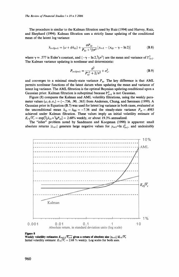
The Review of Financial Studies I v 19 n 3 2006
The procedure is similar to the Kalman filtration used by Ruiz (1994) and Harvey, Ruiz, and Shephard (1994). Kalman filtration uses a strictly linear updating of the conditional mean of the latent log variance:
xr+i|,+i = (u; + #,|,) + <t>Pt\t Pt\t + l/v?
[yt+i -(x,|f-7-ln2)] (B.8)
where 7 ? .577 is Euler's constant, and (-7 - ln2,V27r2) are the mean and variance of ?2+1. The Kalman variance updating is nonlinear and deterministic:
itf+2/** + 02,, (B.9)
and converges to a minimal steady-state variance Pss. The key difference is that AML
permits nonlinear functions of the latest datum when updating the mean and variance of latent log variance. The AML filtration is the optimal Bayesian updating conditional upon a Gaussian prior. Kalman filtration is suboptimal because e2+1 is not Gaussian.
Figure (8) compares the Kalman and AML volatility filtrations, using the weekly para? meter values (u;, 0,<rv) = (-.736, .90, .363) from Andersen, Chung, and Sorensen (1999). A Gaussian prior in Equation (B.7) was used for latent log variance in both cases, evaluated at the unconditional mean xt\t = 3cq|o = ?7.36 and the steady-state variance Pss = .4985 achieved under Kalman filtration. These values imply an initial volatility estimate of Ety/Vt = exp[1/2Xt\t+1/iPt\t] = 2.68% weekly, or about 19.3% annualized.
The "inlier" problem noted by Sandmann and Koopman (1998) is apparent: small absolute returns \zt+\\ generate large negative values for yt+\=\n z2+l, and undesirably
0.001 0.01 0.1 1 10 Absolute return, in standard deviation units (log scale)
Figure 8 Weekly volatility estimates Et+iy/Vt+i given a return of absolute size \zt+i \/Ety/Vt Initial volatility estimate: EtyfVt = 2.68 % weekly. Log scales for both axes.
960

Latent Affine Processes
large downward revisions in Kalman volatility and log variance estimates. The graph illustrates that the Kalman filter also suffers from an "outlier" problem: it substantially underresponds to returns larger than about two standard deviations. The result is inefficient filtration. On a generated sample of 20,000 weekly observations, Kalman filtration had an R2 of 27% when estimating true volatility y/Vt or log variance ln Vt. By contrast, the AML
volatility and log variance filtrations had substantially higher P2s of 37-38%.
B.2 Parameter estimation efficiency The AML approach potentially suffers some loss of estimation efficiency from its use of normal distributions to summarize what is known about the latent variable at each point in time. For the log variance process in Equation (B.l), the estimation efficiency can be directly compared with EMM, MCMC, and other approaches. The efficiency of those approaches for the log variance process is summarized in Andersen, Chung, and Sorensen (1999).
Table 9 appends to Andersen et al.'s Table 5 the results from simulating 500 independent sample paths from Equation (B.l) and estimating the parameters via AML, for sample
Table 9 Comparison of estimation methodologies for the discrete-time log variance process
r=500 r=2000
Zt+i =y/Vt?t+i ln Vt+i = u + (j) ln Vt + o-vfjt+i ?
ML|V and AML estimates are from 500 Monte Carlo sample paths of 500 and 2000 observations, respectively. Results for all other approaches are from comparable runs summarized in Table 5 of Andersen, Chung, and S0rensen (1999). Models: ML|V: ML conditional upon observing {Vt) AML: approximate ML of this article QML: Harvey, Ruiz and Shephard (1994) MCMC: Jacquier, Poison and Rossi (1994) GMM: Andersen and Sorensen (1996) ML: Fridman and Harris (1998) EMM: Andersen, Chung and Sorensen (1999) MCL: Sandmann and Koopman (1996) aAndersen et al. note that the GMM results for T = 500 are from runs that did not crash, and are therefore not comparable to results from other methods.
961

The Review of Financial Studies I v 19 n 3 2006
sizes of T = 500 and T = 2000 weeks, respectively. In addition, parameters were estimated conditional upon observing the log variance draws (denoted ML|V), as an unattainable bound on parameter estimation efficiency. The AML and ML|V approaches were estimated subject to the constraints |p|<l and a > 0, to ensure stationarity and the existence of an unconditional distribution for the initial observation.
The AML approach is definitely one of the more efficient latent-variable methodologies reported in the table. While Jacquier, Poison, and Rossi's (1994) Monte Carlo Markov Chain
approach has the lowest RMSEs for 2000-observation samples and is close to lowest for 500- observation samples, the RMSEs from AML estimation are almost as small. The AML
approach outperforms Gallant and Tauchen's (2002) EMM approach, which in turn outper- forms the GMM approach of Melino and Turnbull (1990) and the very inefficient Kalman filtrations (QML). AML performs about as well on 500-observation samples as Fridman and Harris's (1998) approach (ML), which also provides filtered estimates of latent volatility.
It may be possible to improve the AML performance further by better approximation methodologies for Gt\t. However, Table 9 suggests that even the simple two-moment Gaussian approximation is close to achieving the Cramer-Rao limit.
References Ait-Sahalia, Y., 2002, "Closed-Form Likelihood Expansions for Multivariate Diffusions," Working Paper 8956, National Bureau of Economic Research, May.
Alizadeh, S., M. W. Brandt, and F. X. Diebold, 2002, "Range-Based Estimation of Stochastic Volatility Models," Journal of Finance, 57, 1047-1091.
Andersen, T. G., L. Benzoni, and J. Lund, 2002, "An Empirical Investigation of Continuous-Time Equity Return Models," Journal ofFinance, 57, 1239-1284.
Andersen, T. G., T. Bollerslev, F. X. Diebold, and H. Ebens, 2001, "The Distribution of Stock Return Volatility," Journal of Financial Economics, 61, 43-76.
Andersen, T. G., H. Chung, and B. E. S0rensen, 1999, "Efficient Method of Moments Estimation ofa Stochastic Volatility Model: A Monte Carlo Study," Journal of Econometrics, 91, 61-87.
Andersen, T. G., and B. E. Sorensen, 1996, "GMM Estimation ofa Stochastic Volatility Model: A Monte Carlo Study," Journal of Business and Economic Statistics, 14, 328-352.
Attari, M., 2004, "Option Pricing Using Fourier Transforms: A Numerically Efficient Simplification," Charles River Associates; available at www.ssra.com.
Bakshi, G, and N. Kapadia, 2003, "Delta-Hedged Gains and the Negative Market Volatility Risk Premium," Review of Financial Studies, 16, 527-566.
Bakshi, G., and D. B. Madan, 2000, "Spanning and Derivative-Security Valuation," Journal of Financial Economics, 55, 205-238.
Barndorff-Nielsen, O. E., and D. R. Cox, 1989, Asymptotic Techniques for Use in Statistics, Chapman and Hall, New York.
Barone-Adesi, G., and R. E. Whaley, 1987, "Efficient Analytic Approximation of American Option Values," Journal of Finance, 42, 301-320.
Bartlett, M. S., 1938, "The Characteristic Function of a Conditional Statistic," The Journal of the London Mathematical Society, 13, 63-67.
Bates, D. S., 1991, "The Crash of'87: Was It Expected? The Evidence from Options Markets," Journal of Finance, 46, 1009-1044.
Bates, D. S., 1996, "Jumps and Stochastic Volatility: Exchange Rate Processes Implicit in PHLX Deutschemark Options," Review of Financial Studies, 9, 69-107.
962

Latent Affine Processes
Bates, D. S., 2000, "Post-'87 Crash Fears in the S&P 500 Futures Option Market," Journal of Econo- metrics, 94, 181-238.
Bates, D. S., 2001, "The Market for Crash Risk," working Paper 8557, National Bureau of Economic Research, October.
Bates, D. S., and R. Craine, 1999, "Valuing the Futures Market Clearinghouse's Default Exposure during the 1987 Crash," Journal of Money, Credit, and Banking, 31, 248-272.
Bliss, R. R., and N. Panigirtzoglou, 2004, "Option-Implied Risk Aversion Estimates," Journal of Finance, 59, 407^46.
Carr, P., H. Geman, D. B. Madan, and M. Yor, 2003, "Stochastic Volatility for Levy Processes," Mathematical Finance, 13, 345-382.
Carr, P., and D. B. Madan, 2000, "Option Valuation Using the Fast Fourier Transform," Journal of Computational Finance, 2, 61-73.
Carrasco, M. et al., 2002, "Efficient Estimation of Jump Diffusions and General Dynamic Models with a Continuum of Moment Conditions," University of North Carolina.
Chacko, G., and L. M. Viceira, 2003, "Spectral GMM Estimation of Continuous-time Processes," Journal of Econometrics, 116, 259-292.
Chernov, M., et al., 2003, "Alternative Models for Stock Price Dynamics," Journal of Econometrics, 116, 225-257.
Coval, J. D., and T. Shumway, 2001, "Expected Option Returns," Journal of Finance, 56, 983-1009.
Cumby, R. E., and J. D. Glen, 1990, "Evaluating the Performance of International Mutual Funds," Journal of Finance, 45, 497-521.
Duffie, D., J. Pan, and K. J. Singleton, 2000, "Transform Analysis and Asset Pricing for Affine Jump- Diffusions," Econometrica, 68, 1343-1376.
Duffie, D., and K. J. Singleton, 1993, "Simulated Moments Estimation of Markov Models of Asset Prices," Econometrica, 61, 929-952.
Durham, G. B., and A. R. Gallant, 2002, "Numerical Techniques for Maximum Likelihood Estimation of Continuous-Time Diffusion Processes," Journal of Business and Economic Statistics, 20, 297-316.
Eden, R., 1555, The Decades ofthe neue worlde or west India, conteynyng the nauigations and conquestes of the Spanyardes, with the particular description ofthe moste ryche and large landes and Ilandes lately founde in the west Ocean, perteynyng to the inheritaunce ofthe kinges of Spayne, Rycharde Jug, London.
Eraker, B., M. Johannes, and N. G. Poison, 2003, "The Impact of Jumps in Volatility and Returns," Journal of Finance, 58, 1269-1300.
Feuerverger, A., 1990, "An Efficiency Result for the Empirical Characteristic Function in Stationary Time-Series Models," The Canadian Journal of Statistics, 18, 155-161.
Feuerverger, A., and P. McDunnough, 1981a, "On Some Fourier Methods for Inference," Journal ofthe American Statistical Association, 76, 379-387.
Feuerverger, A., and P. McDunnough, 1981b, "On the Efficiency of Empirical Characteristic Function Procedures," Journal ofthe Royal Statistics Society, Series B, 43, 20-27.
Fleming, J., and C. Kirby, 2003, "A Closer Look at the Relation between GARCH and Stochastic Autoregressive Volatility," Journal of Financial Econometrics, 1, 365-419.
Fridman, M., and L. Harris, 1998, "A Maximum Likelihood Approach for Non-Gaussian Stochastic Volatility Models," Journal of Business and Economic Statistics, 16, 284-291.
Gallant, A. R., and G. Tauchen, 1998, "Reprojecting Partially Observed Systems With Application to Interest Rate Diffusions," Journal ofthe American Statistical Association, 93, 10-24.
963
The Review of Financial Studies I v 19 n 3 2006
Gallant, A. R., and G. Tauchen, 2002, "Simulated Score Methods and Indirect Inference for Continuous- Time Models," University of North Carolina.
Goetzmann, W. N., J. E. Ingersoll, Jr., M. Spiegel, and I. Welch, 2002, "Sharpening Sharpe Ratios," Working Paper 9116, National Bureau of Economic Research, August.
Hamilton, J. D., 1994, Time Series Analysis, Princeton University Press, Princeton, NJ.
Harvey, A., E. Ruiz, and N. Shephard, 1994, "Multivariate Stochastic Variance Models," Review of Economic Studies, 61, 247-264.
Hentschel, L., 1995, "All in the Family: Nesting Symmetric and Asymmetric GARCH Models," Journal of Financial Economics, 39, 71-104.
Ho, M. S., W. R. M. Perraudin, and B. E. Sorensen, 1996, "A Continuous Time Arbitrage Pricing Model with Stochastic Volatility and Jumps," Journal of Business and Economic Statistics, 14, 31-43.
Honore, P., 1998, "Pitfalls in Estimating Jump-Diffusion Models," Aarhus School of Business.
Huang, J. and L. Wu, 2004, "Specification Analysis of Option Pricing Models Based on Time-Changed Levy Processes," Journal of Finance, 59, 1405-1439.
Jacquier, E., N. G. Poison, and P. E. Rossi, 1994, "Bayesian Analysis of Stochastic Volatility Models," Journal of Business and Economic Statistics, 12, 1-19.
Jegadeesh, N., and G Pennacchi, 1996, "The Behavior of Interest Rates Implied by the Term Structure of Eurodollar Futures," Journal of Money, Credit, and Banking, 28, 426-446.
Jiang, G. J., and J. L. Knight, 2002, "Estimation of Continuous Time Processes Via the Empirical Characteristic Function," Journal of Business and Economic Statistics, 20, 198-212.
Johannes, M., N. G. Poison, and J. Stroud, 2002, "Nonlinear Filtering of Stochastic Differential Equations with Jumps," Columbia University
Judd, K. L., 1998, Numerical Methods in Economics, MIT Press, Cambridge (MA).
Karlin, S. and H. M. Taylor, 1981, A Second Course in Stochastic Processes, Academic Press, Boston.
Kolassa, J. E., 1997, Series Approximation Methods in Statistics, Springer-Verlag, New York.
Lewis, A. L., 2001, "A Simple Option Formula for General Jump-Diffusion and Other Exponential Levy Processes," Environ Financial Systems.
Liu, J., J. Pan, and T. Wang, 2004, "An Equilibrium Model of Rare Event Premia," Review of Financial Studies, 18, 131-164.
Lo, A. W., 1988, "Maximum Likelihood Estimation of Generalized Ito Processes with Discretely Sampled Data," Econometric Theory, 4, 231-247.
McFadden, D., 1989, "A Method of Simulated Moments for Estimation of Discrete Response Models without Numerical Integration," Econometrica, 57, 995-1026.
Melino, A., and S. M. Turnbull, 1990, "Pricing Foreign Currency Options with Stochastic Volatility," Journal of Econometrics, 45, 239-265.
Nankervis, J. C, and N. E. Savin, 1988, "The Exact Moments ofthe Least-Squares Estimator for the Autoregressive Model: Corrections and Extensions," Journal of Econometrics, 37, 381-388.
Nelson, D. B., 1992, "Filtering and Forecasting with Misspecified ARCH Models I: Getting the Right Variance with the Wrong Model," Journal of Econometrics, 52, 61-90.
Nelson, D. B., and D. P. Foster, 1994, "Asymptotic Filtering Theory for Univariate ARCH Models," Econometrica, 62, 1-41.
964
Latent Affine Processes
Pan, J., 2002, "The Jump-Risk Premia Implicit in Options: Evidence from an Integrated Time-Series Study," Journal of Financial Economics, 63, 3-50.
Pearson, K., 1933, "On a Method of Determining whether a Sample of Size n Supposed to Have Been Drawn from a Parent Population Having a Known Probability Integral has Probably Been Drawn at Random," Biometrika, 25, 379-410.
Pearson, N. D., and T. Sun, 1994, "Exploiting the Conditional Density in Estimating the Term Structure: An Application to the Cox, Ingersoll, and Ross Model," Journal of Finance, 49, 1279-1304.
Press, W. H. et al, 1992, Numerical Recipes in FORTRAN: The Art of Scientific Computing (2nd ed.), Cambridge University Press, Cambridge.
Rosenberg, J., and R. F. Engle, 2002, "Empirical Pricing Kernels," Journal of Financial Economics, 64, 341-372.
Ruiz, E., 1994, "Quasi-Maximum Likelihood Estimation of Stochastic Volatility Models," Journal of Econometrics, 63, 289-306.
Sandmann, G, and S. J. Koopman, 1998, "Estimation of Stochastic Volatility Models via Monte Carlo Maximum Likelihood," Journal of Econometrics, 87, 271-301.
Singleton, K. J., 2001, "Estimation of Affine Asset Pricing Models Using the Empirical Characteristic Function," Journal of Econometrics, 102, 111-141.
Stambaugh, R. F., 1999, "Predictive Regressions," Journal of Financial Economics, 54, 375?421.
965


![CONSUMPTION AND PORTFOLIO DECISIONS WHEN ...pages.stern.nyu.edu/~dbackus/GE_asset_pricing...ity on portfolio choice. Kim and Omberg [1996] work with a similar framework but, by assuming](https://img.dokumen.tips/doc/110x75/5f02e09c7e708231d406745f/consumption-and-portfolio-decisions-when-pagessternnyuedudbackusgeassetpricing.jpg)