A bound for the number of different basic solutions

generated by the simplex method (Tomonari Kitahara · Shinji Mizuno)

Math. Program., Ser. A (2013) 137:579–586

The Simplex and Policy-Iteration Methods are

Strongly Polynomial for the Markov Decision

Problem with Fixed Discount (Yinyu Ye)

MATHEMATICS OF OPERATIONS RESEARCH

Vol. 36, No. 4, November 2011, pp. 593–603

RZ Abd Aziz (D1)

• Introductions

• Simplex Method for LP

• Analysis

• Markov Decision Problem

• Conclusion

2

Contents

• Introductions

• Simplex Method for LP

• Analysis

• Markov Decision Problem

• Conclusion

3

Next Section

Introduction

• The simplex method for LP was originally developed by Dantzig.

• In practice, the policy-iteration method, including the simple

policy-iteration or Simplex method, has been remarkably

successful and shown to be most effective and widely used.

• In spite of the practical efficiency of the simplex method, do not

have any good bound for the number of iterations (the bound

was only the number of bases 𝑛!

𝑚! 𝑛−𝑚 !).

4

Introduction

• Klee and Minty showed that the simplex method needs an

exponential number of iterations for an elaborately designed

problem LP.

• Melekopoglou and Condon (1990) showed that a simple policy-

iteration method, with the smallest index pivoting rule, needs

an exponential number of iterations for solving an MDP

problem regardless of discount rates.

5

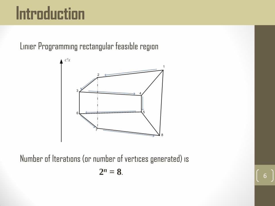
Introduction

Linier Programming rectangular feasible region

Number of Iterations (or number of vertices generated) is

2n = 8. 6

The number of different basic feasible solutions (BFSs) generated by the

simplex method with Dantzig’s rule (the most negative pivoting rule) is

bounded by

𝑛 𝑚𝛾

𝛿log 𝑚

𝛾

𝛿

where

n : The number of variables

m : The number of constraints

𝛿 , 𝛾 : the minimum and the maximum values of all the positive elements of

primal BFSs

When the primal problem is nondegenerate, it becomes a bound for the

number of iterations. The bound depends only on the constraints of LP 7

Result (Tomonari Kitahara · Shinji Mizuno)

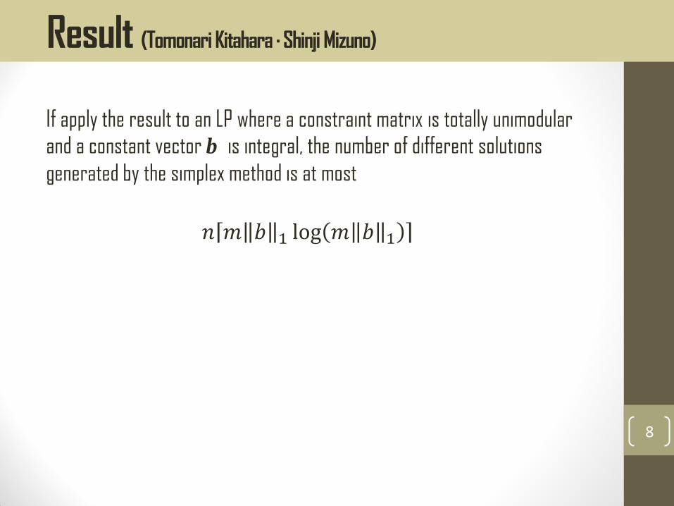
If apply the result to an LP where a constraint matrix is totally unimodular

and a constant vector b is integral, the number of different solutions

generated by the simplex method is at most

𝑛 𝑚 𝑏 1 log 𝑚 𝑏 1

8

Result (Tomonari Kitahara · Shinji Mizuno)

Result (Yinyu Ye)

The classic simplex method, or the simple policy-iteration method, with the greedy

pivoting rule, is a strongly polynomial-time algorithm for MDP with fixed discount

rate:

𝑚2 𝑘 − 1

1 − 𝛾. log

𝑚2

1 − 𝛾

and each iteration uses at most m2k arithmetic operations, where 𝛾 is the fixed

discount rate

In general the number of iterations is bounded by

𝑚2 𝑛 − 𝑚

1 − 𝛾. log

𝑚2

1 − 𝛾

where n is the total number of actions. 9

• Introductions

• Simplex Method for LP

• Analysis

• Markov Decision Problem

• Conclusion

10

Next Section

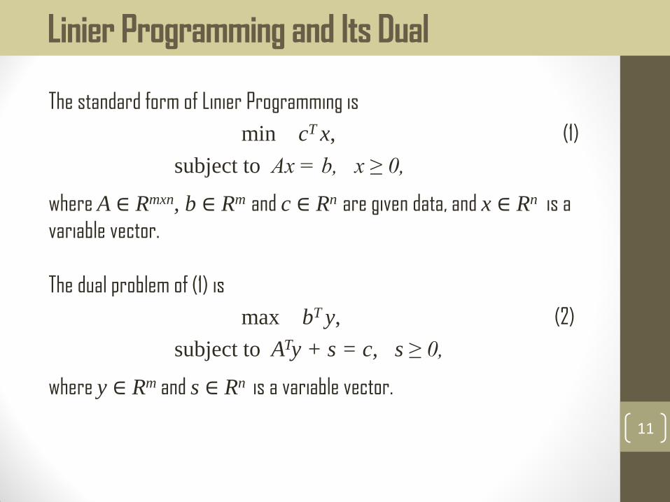
Linier Programming and Its Dual

The standard form of Linier Programming is

min cT x, (1)

subject to Ax = b, x ≥ 0,

where A ∈ Rmxn, b ∈ Rm and c ∈ Rn are given data, and x ∈ Rn is a

variable vector.

The dual problem of (1) is

max bT y, (2)

subject to ATy + s = c, s ≥ 0,

where y ∈ Rm and s ∈ Rn is a variable vector.

11

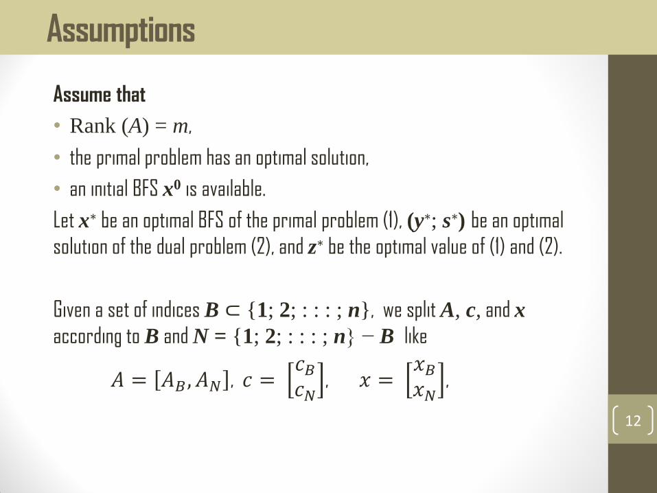
Assumptions

Assume that

• Rank (A) = m,

• the primal problem has an optimal solution,

• an initial BFS x0 is available.

Let x∗ be an optimal BFS of the primal problem (1), (y∗; s∗) be an optimal

solution of the dual problem (2), and z∗ be the optimal value of (1) and (2).

Given a set of indices B ⊂ {1; 2; : : : ; n}, we split A, c, and x according to B and N = {1; 2; : : : ; n} − B like

𝐴 = 𝐴𝐵, 𝐴𝑁 , 𝑐 = 𝑐𝐵

𝑐𝑁, 𝑥 =

𝑥𝐵

𝑥𝑁,

12

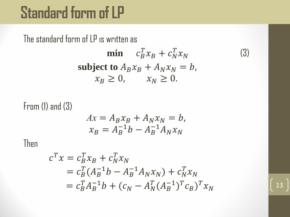
Standard form of LP

The standard form of LP is written as

min 𝑐𝐵𝑇𝑥𝐵 + 𝑐𝑁

𝑇𝑥𝑁 (3)

subject to 𝐴𝐵𝑥𝐵 + 𝐴𝑁𝑥𝑁 = 𝑏, 𝑥𝐵 ≥ 0, 𝑥𝑁 ≥ 0.

From (1) and (3) Ax = 𝐴𝐵𝑥𝐵 + 𝐴𝑁𝑥𝑁 = 𝑏, 𝑥𝐵 = 𝐴𝐵

−1𝑏 − 𝐴𝐵−1𝐴𝑁𝑥𝑁

Then

𝑐𝑇𝑥 = 𝑐𝐵𝑇𝑥𝐵 + 𝑐𝑁

𝑇𝑥𝑁

= 𝑐𝐵𝑇(𝐴𝐵

−1𝑏 − 𝐴𝐵−1𝐴𝑁𝑥𝑁) + 𝑐𝑁

𝑇𝑥𝑁

= 𝑐𝐵𝑇𝐴𝐵

−1𝑏 + (𝑐𝑁 − 𝐴𝑁𝑇 (𝐴𝐵

−1)𝑇𝑐𝐵)𝑇𝑥𝑁

13

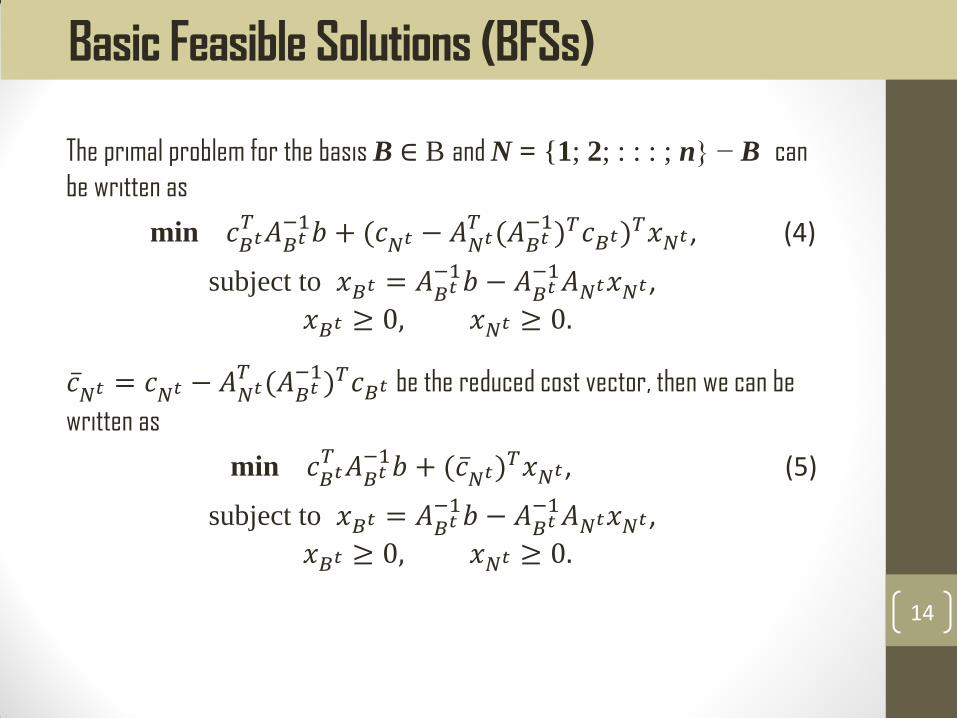
The primal problem for the basis B ∈ B and N = {1; 2; : : : ; n} − B can

be written as

min 𝑐𝐵𝑡𝑇 𝐴𝐵𝑡

−1𝑏 + (𝑐𝑁𝑡 − 𝐴𝑁𝑡𝑇 (𝐴𝐵𝑡

−1)𝑇𝑐𝐵𝑡)𝑇𝑥𝑁𝑡 , (4)

subject to 𝑥𝐵𝑡 = 𝐴𝐵𝑡−1𝑏 − 𝐴𝐵𝑡

−1𝐴𝑁𝑡𝑥𝑁𝑡 ,

𝑥𝐵𝑡 ≥ 0, 𝑥𝑁𝑡 ≥ 0.

𝑐 𝑁𝑡 = 𝑐𝑁𝑡 − 𝐴𝑁𝑡𝑇 (𝐴𝐵𝑡

−1)𝑇𝑐𝐵𝑡 be the reduced cost vector, then we can be

written as

min 𝑐𝐵𝑡𝑇 𝐴𝐵𝑡

−1𝑏 + (𝑐 𝑁𝑡)𝑇𝑥𝑁𝑡 , (5)

subject to 𝑥𝐵𝑡 = 𝐴𝐵𝑡−1𝑏 − 𝐴𝐵𝑡

−1𝐴𝑁𝑡𝑥𝑁𝑡 ,

𝑥𝐵𝑡 ≥ 0, 𝑥𝑁𝑡 ≥ 0.

14

Basic Feasible Solutions (BFSs)

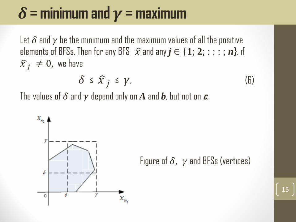
Let 𝛿 and 𝛾 be the minimum and the maximum values of all the positive elements of BFSs. Then for any BFS 𝑥 and any j ∈ {1; 2; : : : ; n}, if

𝑥 𝑗 ≠ 0, we have

𝛿 ≤ 𝑥 𝑗 ≤ 𝛾, (6)

The values of 𝛿 and 𝛾 depend only on A and b, but not on c.

15

𝜹 = minimum and 𝜸 = maximum

Figure of 𝛿, 𝛾 and BFSs (vertices)

When 𝑐 𝑁𝑡 ≥ 0, the current solution is optimal. Otherwise we conduct a

pivot. Under the most negative rule, we choose a nonbasic variable whose

reduced cost is minimum, i.e., we choose an index

j 𝑡

= arg min𝑗∈𝑁𝑡

𝑐j

Set ∆𝑡= −𝑐 j 𝑡 > 0, that is, −∆𝑡 is the minimum value of the reduced

costs

16

Pivoting rule

x* : An optimal basic feasible solution of (1)

(y*; s*): An optimal solution of (2)

z* : The optimal value (1) and (2)

xt : The t-th iterate of the simplex method

Bt : The basis of xt

Nt : The nonbasis of xt

𝑐 𝑁𝑡 : The reduced cost vector at t-th iteration

∆𝑡 : −min𝑗∈𝑁𝑡

𝑐j

j 𝑡 : An index chosen by most negative at t-th iteration 17

Notations

Lemma 1 Let z* be the optimal value of problem (1) and xt be the t-th iterate generated by the simplex method with the most negative rule. Then we have

𝒛∗ ≥ 𝒄𝑻𝒙𝒕 − ∆𝒕𝒎𝜸. (7)

18

A lower bound of Optimal Value of Simplex method

min 𝑐𝐵𝑡𝑇 𝐴𝐵𝑡

−1𝑏 + (𝑐 𝑁𝑡)𝑇

subject to 𝑥𝐵𝑡 = 𝐴𝐵𝑡−1𝑏 − 𝐴𝐵𝑡

−1𝐴𝑁𝑡𝑥𝑁𝑡,

𝑥𝐵𝑡 ≥ 0, 𝑥𝑁𝑡 ≥ 0.

• Introductions

• Simplex Method for LP

• Analysis

• Markov Decision Problem

• Conclusion

19

Next Section

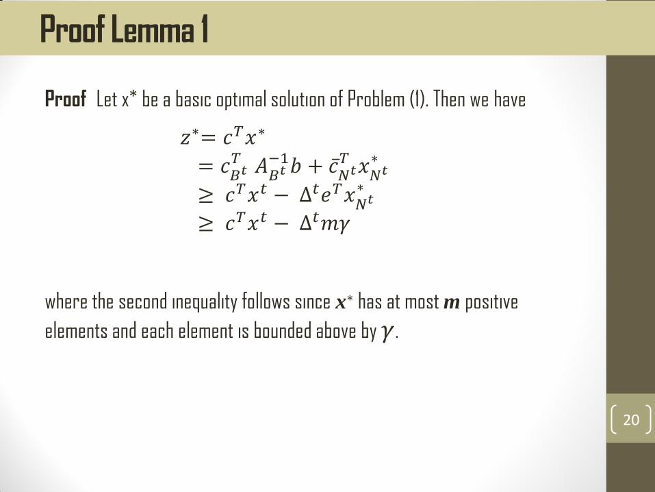
Proof Let x* be a basic optimal solution of Problem (1). Then we have

where the second inequality follows since x∗ has at most m positive

elements and each element is bounded above by 𝛾.

20

Proof Lemma 1

𝑧∗= 𝑐𝑇𝑥∗

= 𝑐𝐵𝑡𝑇 𝐴𝐵𝑡

−1𝑏 + 𝑐 𝑁𝑡𝑇 𝑥𝑁𝑡

∗

≥ 𝑐𝑇𝑥𝑡 − ∆𝑡𝑒𝑇𝑥𝑁𝑡∗

≥ 𝑐𝑇𝑥𝑡 − ∆𝑡𝑚𝛾

A constant reduction of the gap (𝒄𝑻𝒙𝒕 − 𝒛∗) whenban iterate is updated.

The reduction rate 1 −𝛿

𝑚𝛾 does not dependent on the objective vector c.

Theorem 1 Let xt and xt+1 be the t-th and (t + 1)-th iterates generated by the simplex method with the most negative rule. If xt+1 , xt , then we have

𝒄𝑻𝒙𝒕+𝟏 − 𝒛∗ ≤ 1 −𝛿

𝑚𝛾𝒄𝑻𝒙𝒕 − 𝒛∗ . (8)

21

Reduction Rate (Theorem 1)

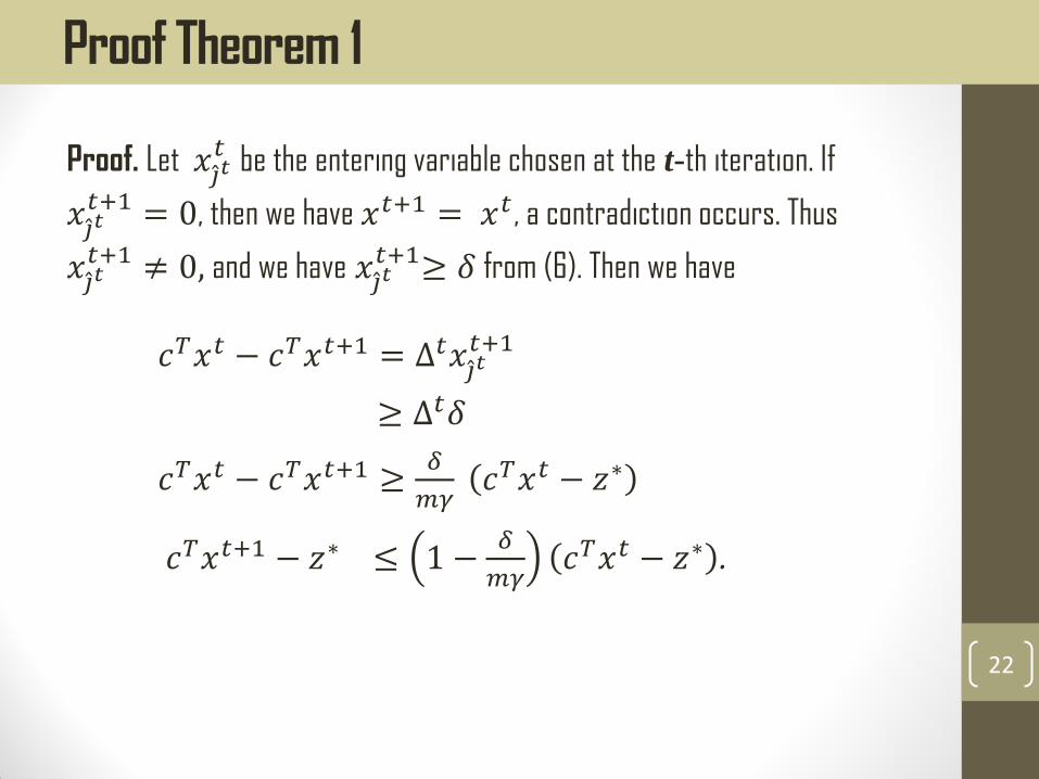
Proof. Let 𝑥𝑗 𝑡𝑡 be the entering variable chosen at the t-th iteration. If

𝑥𝑗 𝑡𝑡+1 = 0, then we have 𝑥𝑡+1 = 𝑥𝑡 , a contradiction occurs. Thus

𝑥𝑗 𝑡𝑡+1 ≠ 0, and we have 𝑥𝑗 𝑡

𝑡+1≥ 𝛿 from (6). Then we have

𝑐𝑇𝑥𝑡 − 𝑐𝑇𝑥𝑡+1 = ∆𝑡𝑥𝑗 𝑡𝑡+1

≥ ∆𝑡𝛿

𝑐𝑇𝑥𝑡 − 𝑐𝑇𝑥𝑡+1 ≥𝛿

𝑚𝛾 𝑐𝑇𝑥𝑡 − 𝑧∗

𝑐𝑇𝑥𝑡+1 − 𝑧∗ ≤ 1 −𝛿

𝑚𝛾𝑐𝑇𝑥𝑡 − 𝑧∗ .

22

Proof Theorem 1

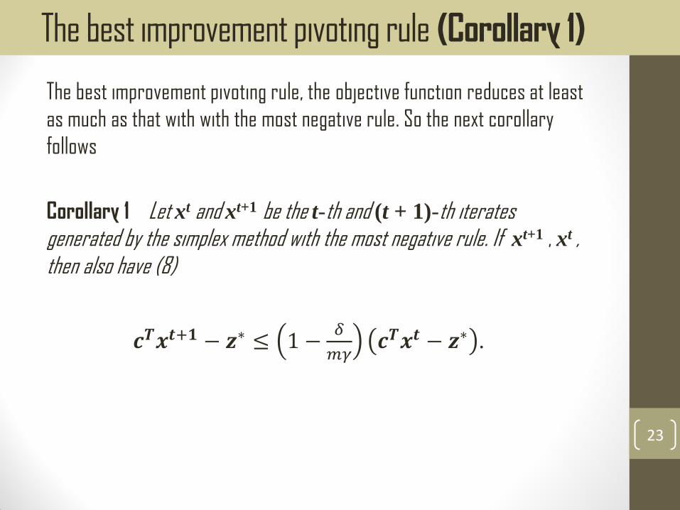
The best improvement pivoting rule, the objective function reduces at least

as much as that with with the most negative rule. So the next corollary

follows

Corollary 1 Let xt and xt+1 be the t-th and (t + 1)-th iterates generated by the simplex method with the most negative rule. If xt+1 , xt , then also have (8)

𝒄𝑻𝒙𝒕+𝟏 − 𝒛∗ ≤ 1 −𝛿

𝑚𝛾𝒄𝑻𝒙𝒕 − 𝒛∗ .

23

The best improvement pivoting rule (Corollary 1)

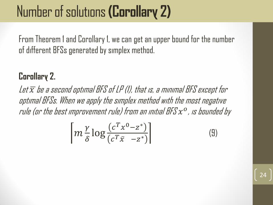
From Theorem 1 and Corollary 1, we can get an upper bound for the number

of different BFSs generated by simplex method.

Corollary 2.

Let 𝑥 be a second optimal BFS of LP (1), that is, a minimal BFS except for optimal BFSs. When we apply the simplex method with the most negative rule (or the best improvement rule) from an initial BFS 𝑥𝑜 , is bounded by

𝑚𝛾

𝛿log

𝑐𝑇𝑥0−𝑧∗

𝑐𝑇𝑥 −𝑧∗ (9)

24

Number of solutions (Corollary 2)

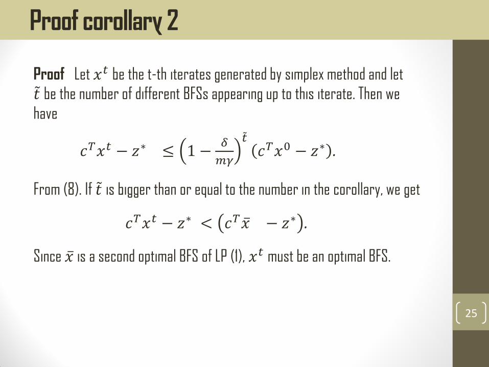
Proof Let 𝑥𝑡 be the t-th iterates generated by simplex method and let

𝑡 be the number of different BFSs appearing up to this iterate. Then we

have

𝑐𝑇𝑥𝑡 − 𝑧∗ ≤ 1 −𝛿

𝑚𝛾

𝑡

𝑐𝑇𝑥0 − 𝑧∗ .

From (8). If 𝑡 is bigger than or equal to the number in the corollary, we get

𝑐𝑇𝑥𝑡 − 𝑧∗ < 𝑐𝑇𝑥 − 𝑧∗ .

Since 𝑥 is a second optimal BFS of LP (1), 𝑥𝑡 must be an optimal BFS.

25

Proof corollary 2

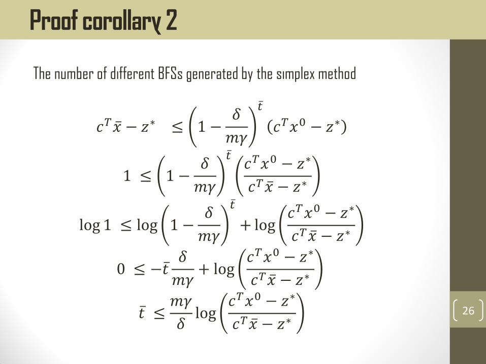
The number of different BFSs generated by the simplex method

𝑐𝑇𝑥 − 𝑧∗ ≤ 1 −𝛿

𝑚𝛾

𝑡

𝑐𝑇𝑥0 − 𝑧∗

1 ≤ 1 −𝛿

𝑚𝛾

𝑡 𝑐𝑇𝑥0 − 𝑧∗

𝑐𝑇𝑥 − 𝑧∗

log 1 ≤ log 1 −𝛿

𝑚𝛾

𝑡

+ log𝑐𝑇𝑥0 − 𝑧∗

𝑐𝑇𝑥 − 𝑧∗

0 ≤ −𝑡 𝛿

𝑚𝛾+ log

𝑐𝑇𝑥0 − 𝑧∗

𝑐𝑇𝑥 − 𝑧∗

𝑡 ≤𝑚𝛾

𝛿log

𝑐𝑇𝑥0 − 𝑧∗

𝑐𝑇𝑥 − 𝑧∗

26

Proof corollary 2

If the current solution is not optimal, there is a basic variable which has an

upper bound proportional to the gap between the objective value and the

optimal value

Lemma 2 Let 𝑥𝑡 be t-th iterate generate by simplex method. If 𝑥𝑡 is not

optimal, there exists j ∈ 𝐵𝑡 such that 𝑥j 𝑡 > 0 and

𝑥j 𝑘 ≤

𝑚 𝑐𝑇𝑥𝑘−𝑧∗

𝑐𝑇𝑥𝑡−𝑧∗ 𝑥j 𝑡 (10)

For any feasible solution x.

27

An Upper Bound proportional gap (Lemma 2)

An Upper Bound proportional gap (Lemma 2)

min 𝑐𝐵∗𝑇 𝐴𝐵∗

−1𝑏 + (𝑐 𝑁∗)𝑇

subject to 𝑥𝐵𝑡 = 𝐴𝐵∗−1𝑏 − 𝐴𝐵∗

−1𝐴𝑁∗𝑥𝑁∗ , 𝑥𝐵𝑡 ≥ 0, 𝑥𝑁𝑡 ≥ 0.

𝑥j 𝑘 ≤

𝑚 𝑐𝑇𝑥𝑘 − 𝑧∗

𝑐𝑇𝑥𝑡 − 𝑧∗𝑥j

𝑡

28

Proof. From primal (1) and dual (2), we have

𝑐𝑇𝑥𝑡 − 𝑧∗ = 𝑐𝑇𝑥𝑡 − 𝑏𝑇𝑦∗

= 𝑥𝑡 𝑇𝑐 − 𝑥𝑡 𝑇𝐴𝑇𝑦∗

= 𝑥𝑡 𝑇 𝑐 − 𝐴𝑇𝑦∗

= 𝑥𝑡 𝑇𝑠∗ = 𝑥𝑡𝑠𝑗∗

𝑗∈𝐵𝑡

There exists j ∈ 𝐵𝑡 which satisfies

𝑐𝑇𝑥𝑡 − 𝑧∗ = 𝑥𝑡 𝑇𝑠∗ ≤ 𝑚𝑥j 𝑡𝑠j

∗

𝑚𝑥j 𝑡𝑠j

∗ ≥ 𝑐𝑇𝑥𝑡 − 𝑧∗

𝑠j ∗ ≥

1

𝑚𝑥j 𝑡 𝑐𝑇𝑥𝑡 − 𝑧∗

29

Proof Lemma 2

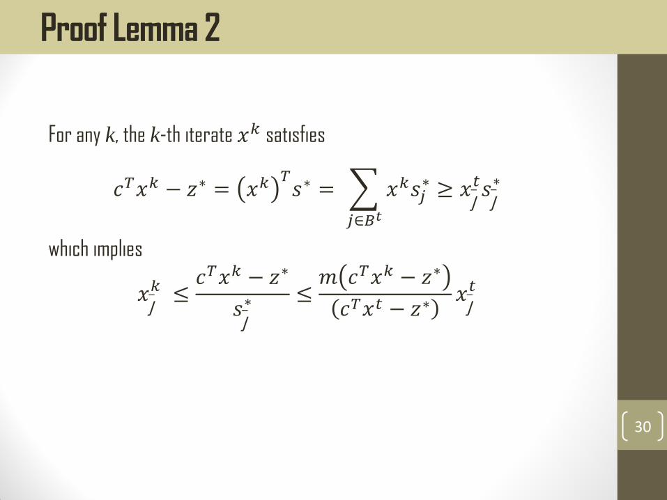
For any k, the k-th iterate 𝑥𝑘 satisfies

𝑐𝑇𝑥𝑘 − 𝑧∗ = 𝑥𝑘 𝑇𝑠∗ = 𝑥𝑘𝑠𝑗

∗

𝑗∈𝐵𝑡

≥ 𝑥j 𝑡𝑠j

∗

which implies

𝑥j 𝑘 ≤

𝑐𝑇𝑥𝑘 − 𝑧∗

𝑠j ∗ ≤

𝑚 𝑐𝑇𝑥𝑘 − 𝑧∗

𝑐𝑇𝑥𝑡 − 𝑧∗𝑥j

𝑡

30

Proof Lemma 2

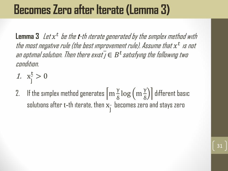
Lemma 3 Let 𝑥𝑡 be the t-th iterate generated by the simplex method with the most negative rule (the best improvement rule). Assume that 𝑥𝑡 is not an optimal solution. Then there exist j ∈ 𝐵𝑡satisfying the following two condition.

1. xj t > 0

2. If the simplex method generates mγ

δlog m

γ

δ different basic

solutions after t-th iterate, then xj becomes zero and stays zero

31

Becomes Zero after Iterate (Lemma 3)

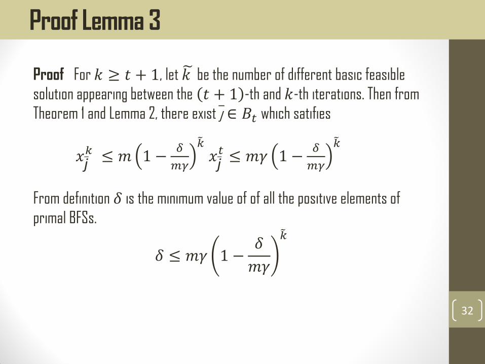
Proof For 𝑘 ≥ 𝑡 + 1, let 𝑘 be the number of different basic feasible

solution appearing between the 𝑡 + 1 -th and 𝑘-th iterations. Then from

Theorem 1 and Lemma 2, there exist j ∈ 𝐵𝑡 which satifies

𝑥j 𝑘 ≤ 𝑚 1 −

𝛿

𝑚𝛾

𝑘

𝑥j 𝑡 ≤ 𝑚𝛾 1 −

𝛿

𝑚𝛾

𝑘

From definition 𝛿 is the minimum value of of all the positive elements of

primal BFSs.

𝛿 ≤ 𝑚𝛾 1 −𝛿

𝑚𝛾

𝑘

32

Proof Lemma 3

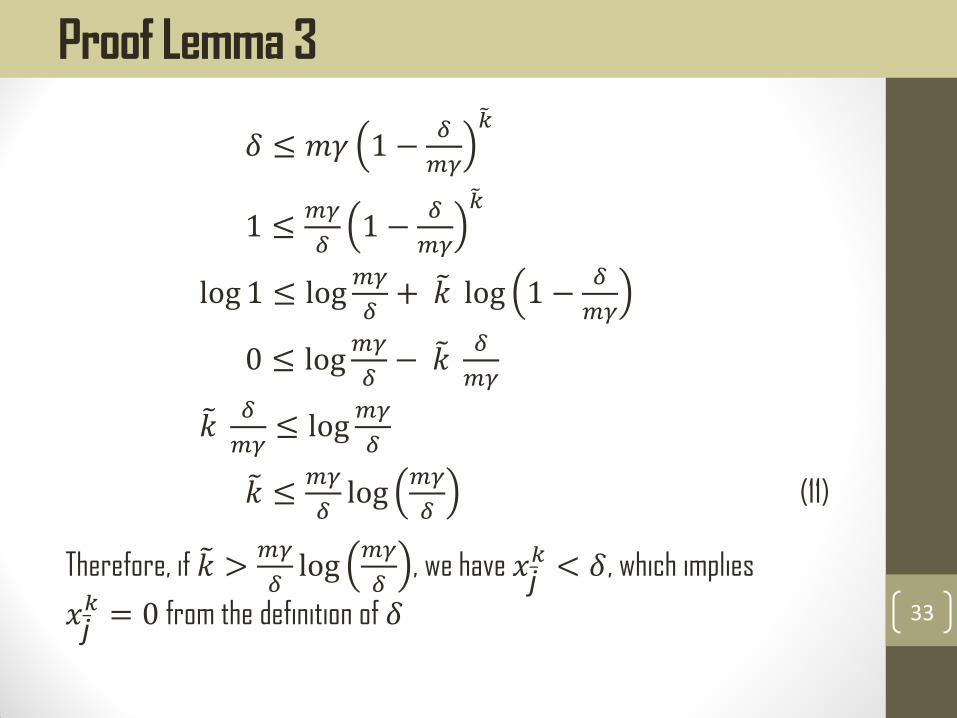
𝛿 ≤ 𝑚𝛾 1 −𝛿

𝑚𝛾

𝑘

1 ≤𝑚𝛾

𝛿1 −

𝛿

𝑚𝛾

𝑘

log 1 ≤ log𝑚𝛾

𝛿+ 𝑘 log 1 −

𝛿

𝑚𝛾

0 ≤ log𝑚𝛾

𝛿− 𝑘

𝛿

𝑚𝛾

𝑘 𝛿

𝑚𝛾≤ log

𝑚𝛾

𝛿

𝑘 ≤𝑚𝛾

𝛿log

𝑚𝛾

𝛿 (11)

Therefore, if 𝑘 >𝑚𝛾

𝛿log

𝑚𝛾

𝛿, we have 𝑥j

𝑘 < 𝛿, which implies

𝑥j 𝑘 = 0 from the definition of 𝛿

33

Proof Lemma 3

The event described in Lemma 3 can occur at most once for each variable.

Thus we get the following result

Theorem 2 when we apply the simplex method with the most negative rule (the best improvement rule for LP (1) having optimal solutions, we encounter at most

n𝑚𝛾

𝛿log

𝑚𝛾

𝛿 (12)

different basic feasible solutions.

34

Bound for the Number of Solutions (Theorem 2)

Note that the result is valid even if the simplex method fails to find an

optimal solution because of a cycling

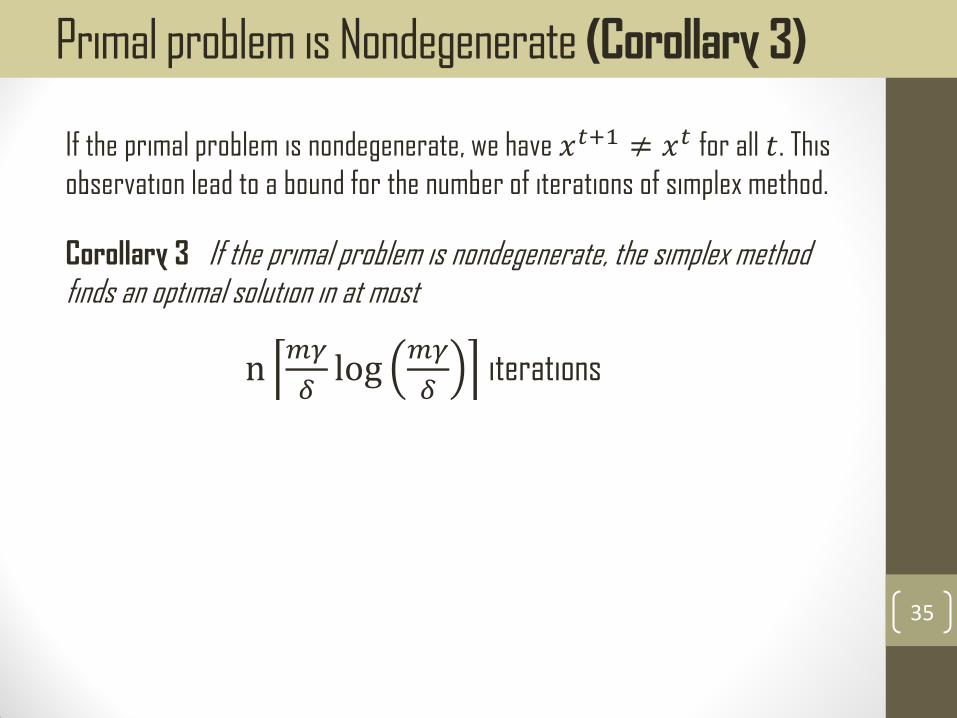
If the primal problem is nondegenerate, we have 𝑥𝑡+1 ≠ 𝑥𝑡 for all 𝑡. This

observation lead to a bound for the number of iterations of simplex method.

Corollary 3 If the primal problem is nondegenerate, the simplex method finds an optimal solution in at most

n𝑚𝛾

𝛿log

𝑚𝛾

𝛿 iterations

35

Primal problem is Nondegenerate (Corollary 3)

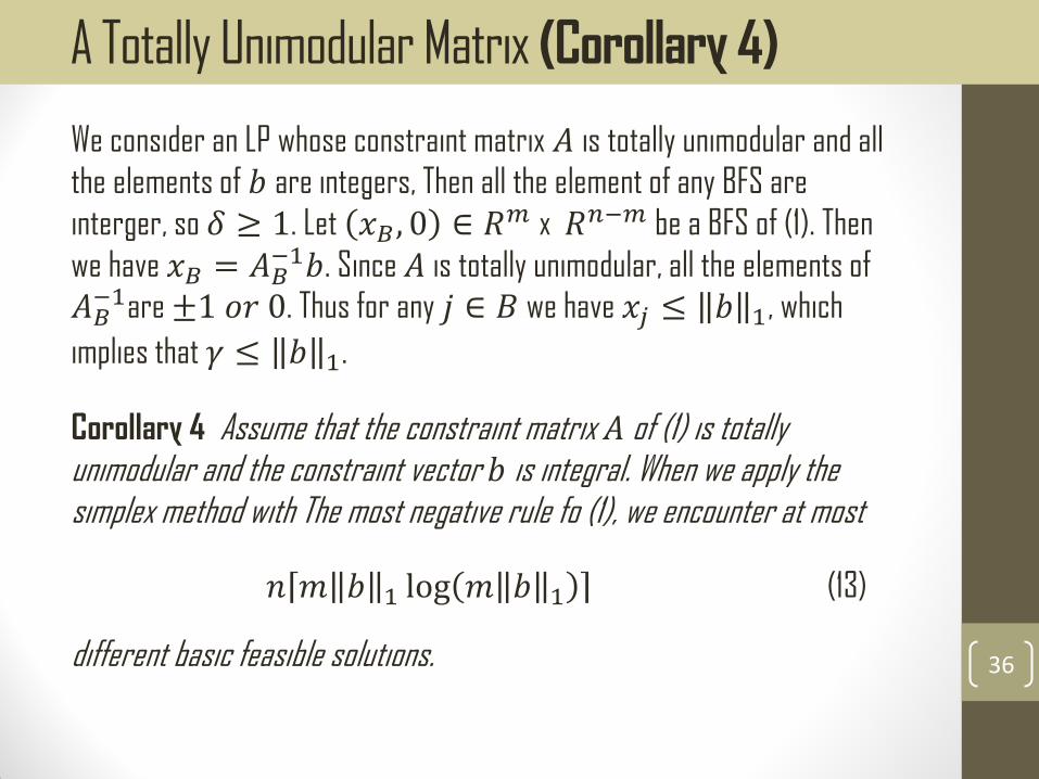
We consider an LP whose constraint matrix 𝐴 is totally unimodular and all

the elements of 𝑏 are integers, Then all the element of any BFS are

interger, so 𝛿 ≥ 1. Let 𝑥𝐵 , 0 ∈ 𝑅𝑚 x 𝑅𝑛−𝑚 be a BFS of (1). Then

we have 𝑥𝐵 = 𝐴𝐵−1𝑏. Since 𝐴 is totally unimodular, all the elements of

𝐴𝐵−1are ±1 𝑜𝑟 0. Thus for any 𝑗 ∈ 𝐵 we have 𝑥𝑗 ≤ 𝑏 1, which

implies that 𝛾 ≤ 𝑏 1.

Corollary 4 Assume that the constraint matrix 𝐴 of (1) is totally unimodular and the constraint vector 𝑏 is integral. When we apply the simplex method with The most negative rule fo (1), we encounter at most

𝑛 𝑚 𝑏 1 log 𝑚 𝑏 1 (13)

different basic feasible solutions.

36

A Totally Unimodular Matrix (Corollary 4)

• Introductions

• Simplex Method for LP

• Analysis

• Markov Decision Problem

• Conclusion

37

Next Section

The Markov Decision Problem (MDP)

min 𝑐1𝑇𝑥1 + 𝑐2

𝑇𝑥2 (14)

subject to 𝐼 − 𝜃𝑃1 𝑥1 + 𝐼 − 𝜃𝑃2 𝑥2 = 𝑒,

𝑥1, 𝑥2 ≥ 0

Where 𝐼 is the 𝑚 x 𝑚 identity matrix, 𝑃1 and 𝑃2 are 𝑚 x 𝑚 Markov

matrices, 𝜃 is a fixed discount rate, and e is the vector of all ones. MDP

(14) has the following properties.

1. MDP (14) is nondegenerate.

2. The minimum value of all the positive elements of BFSs is greater than

or equal to 1, or equivalently, 𝛿 ≥ 1.

3. The maximum value of all the positive elements of BFSs is less than or

equal to 𝑚

1−𝜃 or equivalently, 𝛾 ≤

𝑚

1−𝜃.

38

Markov Decision Problem (MDP)

The result obtain a similar result to (Yinyu Ye)

Corollary 5 The simplex method for solving MDP (14) finds an optimal solution in at most

n𝑚2

1−𝜃𝑙𝑜𝑔

𝑚2

1−𝜃 iterations

where 𝑛 = 2𝑚

Result (Yinyu Ye)

𝑚2 𝑛 − 𝑚

1 − 𝛾. log

𝑚2

1 − 𝛾

39

Number of Iterations for MDP

• Introductions

• Simplex Method for LP

• Analysis

• Markov Decision Problem

• Conclusion

40

Next Section

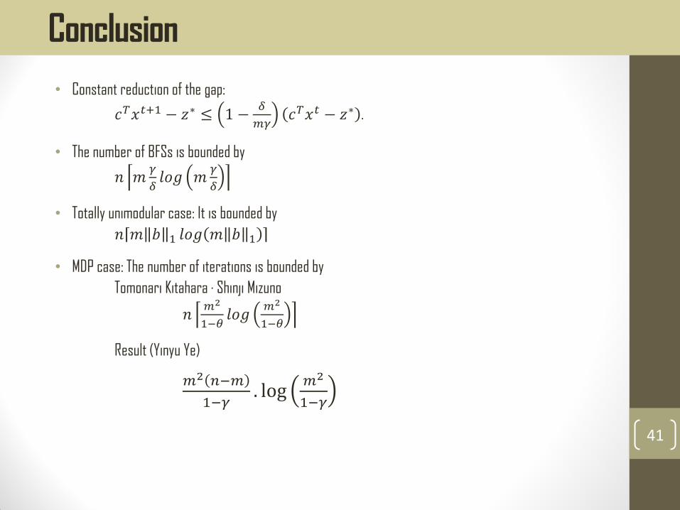
• Constant reduction of the gap:

𝑐𝑇𝑥𝑡+1 − 𝑧∗ ≤ 1 −𝛿

𝑚𝛾𝑐𝑇𝑥𝑡 − 𝑧∗ .

• The number of BFSs is bounded by

𝑛 𝑚𝛾

𝛿𝑙𝑜𝑔 𝑚

𝛾

𝛿

• Totally unimodular case: It is bounded by

𝑛 𝑚 𝑏 1 𝑙𝑜𝑔 𝑚 𝑏 1

• MDP case: The number of iterations is bounded by

Tomonari Kitahara · Shinji Mizuno

𝑛𝑚2

1−𝜃𝑙𝑜𝑔

𝑚2

1−𝜃

Result (Yinyu Ye)

𝑚2 𝑛−𝑚

1−𝛾. log

𝑚2

1−𝛾

41

Conclusion