This article was downloaded by: [USC University of Southern California]On: 04 October 2014, At: 01:51Publisher: Taylor & FrancisInforma Ltd Registered in England and Wales Registered Number: 1072954 Registered office: Mortimer House,37-41 Mortimer Street, London W1T 3JH, UK

Journal of Hydraulic ResearchPublication details, including instructions for authors and subscription information:http://www.tandfonline.com/loi/tjhr20

The significance of single value variables in turbiditycurrentsM. Felix aa Department of Earth Sciences , University of Leeds , Leeds , LS2 9JT , UK E-mail:Published online: 26 Mar 2012.

To cite this article: M. Felix (2004) The significance of single value variables in turbidity currents, Journal of HydraulicResearch, 42:3, 323-330, DOI: 10.1080/00221686.2004.9728398

To link to this article: http://dx.doi.org/10.1080/00221686.2004.9728398

PLEASE SCROLL DOWN FOR ARTICLE

Taylor & Francis makes every effort to ensure the accuracy of all the information (the “Content”) contained in thepublications on our platform. However, Taylor & Francis, our agents, and our licensors make no representationsor warranties whatsoever as to the accuracy, completeness, or suitability for any purpose of the Content. Anyopinions and views expressed in this publication are the opinions and views of the authors, and are not theviews of or endorsed by Taylor & Francis. The accuracy of the Content should not be relied upon and should beindependently verified with primary sources of information. Taylor and Francis shall not be liable for any losses,actions, claims, proceedings, demands, costs, expenses, damages, and other liabilities whatsoever or howsoevercaused arising directly or indirectly in connection with, in relation to or arising out of the use of the Content.

This article may be used for research, teaching, and private study purposes. Any substantial or systematicreproduction, redistribution, reselling, loan, sub-licensing, systematic supply, or distribution in anyform to anyone is expressly forbidden. Terms & Conditions of access and use can be found at http://www.tandfonline.com/page/terms-and-conditions

IAHR~

•~ AJRH

Journal ofHydraulic Research Vol. 42, No.3 (2004), pp. 323-330~ 2004 International Association of Hydraulic Engineering and Researcl

The significance of single value variables in turbidity currents

Signification des variables de valeur simple carateristique dans descourants de turbidite . ,M. FELIX, Department ofEarth Sciences, University ofLeeds, Leeds LS2 9JT. UK. E-mail: mjelix@earth.leeds.ac.uk

, •. f

ABSTRACTA comparison is made between depth-averaged variables and characteristic variables (such as maximum velocity and height of maximum velocity:in natural scale turbidity currents, using a two-dimensional numerical model. These different single value variables are calculated for a range 01simulated turbidity currents and illustrated in more detail for two flows. Single value variables describe the flow structure trend directly for slowl)varying parts of flows, but for rapidly ch~ging parts such variables describe flow only indirectly through momentum and total sediment transport.Different variables indicate the same spatIal development of thickness, velocity and concentration, but only variables that describe totaltranspol1properties (sediment transport and momentum) are similar as their ratios do not vary much between flows. Single value variables cannot be used tcdescribe flow behaviour with derived properties such as Froude numbers, or in equations such as CMzy-type equations.

RESUMEDne comparaison est faite entre les variables moyennes sur la profondeur et les variables caract~ristiques (telles que la vitesse maximum et S2

profondeur) dans les courants de turbidite en nature, en utilisant un mod~le num~rique bidimensionnel. Ces diff~rentes variables de valeur simplecaracteristique sont calculees pour une garnme de courants simules de turbidite et iIIuslrees avec plus de details pour deux ~coulements. Les variablesde valeur simple caracteristique decrivent la tendance de structure de l'ecoulement directement pour les parties d'ecoulements lentement variables,mais pour les parties changeant rapidement de telles variables d6crivent l'ecoulement seulement indirectement par les quantites de mouvement et Ietransport total de sediment. Differentes v~ables indiquent Ie meme developpement spatial de l'epaisseur, de la vitesse et de la concentration, maisseules les variables qui decrivent les propnetes globales de transport (transport de sediment et quantites de mouvement) sont semblables car leursrapports ne changent pas beaucoup avec les ecoulements. Des variables de valeur simple caracteristique ne peuvent pas eire employees pour dccrireIe comportement d'ecoulement avec les proprietes derivees teUes que des nombres de Froude, ou dans les equations telles que celie de Chezy.

Keywords: Single value variables, turbidity currents, depth-averaged variables.

1 Introduction

Quantitative analysis of turbidity currents almost always uses asingle value of flow variables such as velocity or concentration.Using a single value to describe a flow variable greatly simplifiesthe analysis, and the flow behaviour can be easily characterizedby non-dimensional numbers such as ~amongst others) Reynoldsand densiometric Froude numbers (MIddleton, 1966) and can beused in simple equations such as Chezy-type equations (Daly,1936; Kuenen, 1937, 1952). Single value variables can be char-cteristic values such as maximum velocity, nose velocity, visual~ow thickness (based on flow turbidity) or initial sediment con­centration (in the case of lock-release laboratory experiments),Other commonly used single value variables are depth-averagedvariables. which are derived by integrating a vertical profile to

btain a single value describing the variable. Depth-averagedo 'abies are most commonly used in numerical models where~:s are assumed to have ~~prox~alely similar vertical profileshapes at all horizontal pOSItIons 10 the flow, so that the profiles

only differ in magnitude, which is given by the depth-averagedvalue (see e.g. Parker et al., 1986).

Different single value variables have been used for non;dimensionalizing vertical profiles. For example, Garda (1993,1994) and Lee and Yu (1997) used depth-averaged values, whileAltinakar etal. (1996), Buckee etal. (2001) and Felix (2002) usedcharacteristic values. It is unclear whether these different meth­ods result in the same answer and are interchangeable or whethelusing different variables represents different processes so thairesults cannot be compared. It is also unclear to what extent singlevalues can represent the flow behaviour or flow regime as indiocated by, for example, the Froude number. This is especially truefor depth-averaged variables, which are derived from verticall)integrated momentum and concentration. Can these variables Ixused to indicate a specific thickness. velocity or concentratiordirectly or can they only be used indirectly through quantitielsuch as momentum and total sediment transport? Are the differ·ent variables interchangeable ordo they all indicate different flo\\behaviour?

.. n received January 12,2004. Open for discussion till September 30 2004RevIslo ' .

323

Journal ofHydraulic Research Vol. 42, No.3 (2004), pp. 323-330© 2004 International Association of Hydraulic Engineering and Researcl

""'-' A1RH

The significance of single value variables in turbidity currents

Signification des variables de valeur simple carateristique dans descourants de turbidite . . ~. ~ . .". f

M. FELIX, Department ofEarth Sciences, University ofLeeds, Leeds LS2 9JT, UK. E-mail: mje/ix@earth./eeds.ac.uk

ABSTRACTA comparison is made between depth-averaged variables and characteristic variables (such as maximum velocity and height of maximum velocity:in natural scale turbidity currents, using a two-dimensional numerical model. These different single value variables are calculated for a range 01simulated turbidity currents and illustrated in more detail for two flows. Single value variables describe the flow structure trend directly for slowl)varying parts of flows, but for rapidly ch~ging parts such variables describe flow only indirectly through momentum and total sediment transportDifferent variables indicate the same spatIal development of thickness, velocity and concentration, but only variables that describe total transpor1properties (sediment transport and momentum) are similar as their ratios do not vary much between flows. Single value variables cannot be used tcdescribe flow behaviour with derived properties such as Froude numbers, or in equations such as CMzy-type equations.

RESUMEUne comparaison est faite entre les variables moyennes sur la profondeur et les variables caract~ristiques (telles que la vitesse maximum et S2

profondeur) dans les courants de turbidit6 en nature, en utilisant un mod~le num~rique bidimensionnel. Ces diff~rentes variables de valeur simplecaracteristique sont calculees pour une gamme de courants simules de turbidit6 et iIlustrees avec plus de d~tails pour deux ~coulements. Les variablesde valeur simple caracteristique decrivent la tendance de structure de I'ecoulement directement pour les parties d'~coulements lentement variables,mais pour les parties changeant rapidement de telles variables d6crivent I'ecoulement seulement indirectement par les quantites de mouvement et Ietransport total de sedin:'ent. ?ifferentes v~ables indiquent Ie meme developpement sp?tial de l'epais~eur, de la vitesse et de la concentration, maisseules les variables qUI decnvent les propnetes globales de transport (transport de sedIment et quantltes de mouvement) sont semblables car leursrapports ne changent pas beaucoup avec les ecoulements. Des variables de valeur simple caracteristique ne peuvent pas etre employees pour dccrireIe comportement d'ecoulement avec les proprietes derivees telles que des nombres de Froude, ou dans les equations telles que celie de ChCzy.

Keywords: Single value variables, turbidity currents, depth-averaged variables.

1 Introduction

Quantitative analysis of turbidity currents almost always uses asingle value of flow variables such as velocity or concentration.Using a single value to describe a flow variable greatly simplifiesthe analysis, and the flow behaviour can be easily characterizedby non-dimensional numbers such as (amongst others) Reynoldsand densiometric Froude numbers (Middleton, 1966) and can beused in simple equations such as Chezy-type equations (Daly,1936~ Kuenen. 1937, 1952). Single value variables can be char-

teristic values such as maximum velocity, nose velocity, visual~~w thickness (based on flow turbidity) or initial sediment con­centration (in the case of lock-release laboratory experiments).Other commonly used single value variables are depth-averagedvariables, which are derived by integrating a vertical profile to

btain a single value describing the variable. Depth-averagedo .abIes are most commonly used in numerical models where~:s are assumed to have ~~prox~mately similar vertical profileshapes at all horizontal posltlons 10 the flow, so that the profiles

only differ in magnitude, which is given by the depth-averagedvalue (see e.g. Parker et al., 1986).

Different single value variables have been used for non;dimensionalizing vertical profiles. For example, Garda (1993,1994) and Lee and Yu (1997) used depth-averaged values, whileAltinakar erat. (1996), Buckee erat. (2001) and Felix (2002) usedcharacteristic values. It is unclear whether these different meth·ods result in the same answer and are interchangeable or whethelusing different variables represents different processes so thairesults cannot be compared. It is also unclear to what extent singlevalues can represent the flow behaviour or flow regime as indiocated by, for example, the Froude number. This is especially truefor depth-averaged variables, which are derived from verticall)integrated momentum and concentration. Can these variables beused to indicate a specific thickness, velocity or concentratiordirectly or can they only be used indirectly through quanti tie!such as momentum and total sediment transport? Are the differ­ent variables interchangeable ordo they all indicate different flo\\behaviour?

. 'on received January 12,2004. Open for discussion till September 30 2004ReVISI ' •

323

Dow

nloa

ded

by [

USC

Uni

vers

ity o

f So

uthe

rn C

alif

orni

a] a

t 01:

51 0

4 O

ctob

er 2

014

324 Felix

The numerical model of Felix (200 I) is used here to compareseveral single value variables derived from concentration andvelocity to each other and to the flow structure of natural scaleflows. The use of single value variables is illustrated by applyingthe thickness and concentration results to obtain velocities using aChezy-type equation and by determining Froude numbers. Othervariables that can influence flow, such as temperature, salinity,non-zero ambient flow, etc. are not looked at here.

each specific run are topography, initial sediment distri,~~ti?~

(grain sizes and volume fractions) and initial size of the sed­iment column. The equations are solved numerically using afinite volume method with a second order implicit BackwardDifferentiation Formula method. For a complete descriptionof the governing equations and solution method see Fe~i~

(2001). '> rf l'

2 Mathematical model description 3 Determination of single value variables

a0~i"~:;.:~"~"~-;:;";::-:~:.5~'-:::~2~!~2~.5~~~3e1l-~3.5x(km)

3.532.521.50.5

lOa velocity (m/s)

100 concentration

gN 50

The single value variables are determined for the vertical profilesat all horizontal grid points of 36 different runs. This was d~~~

at four different times during the flow development of each run~

giving some tens of thousands of vertical profiles (see below).The initial conditions of the runs systematically varied total ini­tial sediment concentration (3, 15 or 30%), slope (0.5, 2.0?r5.0°) and average grain size (0.1 or 0.5 mm), leading to a total'of3 x 3 x 2 = 18 different input conditions. All of these 18 con­ditions were used for runs on two different domain sizes (initialsediment columns of 50 m long and 15 m high and 500 x75 m)~thus giving a total of 2 x 18 = 36 runs. For illustration pur7poses the analysis is described in more detail for two flows.One flow is a small coarse-grained flow (initial sediment col­umn is SO by 15 m) of initial low concentration of 3%, withaverage grain size of 0.5 mm, and slope OS. The other flowis a large fine-grained flow (initial sediment column is 500 by75 m) of initial high concentration of 30%, with average grainsize 0.1 mm and slope 5°. Flows run down an initial slope ~dthen continue on a horizontal bed (see Figs 1 and 2). These36 runs are used to determine the following depth-averaged and

characteristic variables.

I- H - .... Zll2l

Figure 1 Contour plots for velocity (top) and concentration (bottom)with single value variables shown. Small, low density coarse-grainedflow. Flow is from left to right. Thin lines are contour lines, thick lines

are Hand 2 1/2. Velocity contours are 0.001. 0.01. 0.025. 0.05.0.075and 0.1 m1s. Concentration contours are volumetric fractions 10-8

• 10-7

•

10-6 and 5 x 10-6 • Initial concentration was 3%, initial sediment column

was 50 by 15 m, average grain size is 0.5 mm.

au; -0ax; - ,

The hydrostatic numerical model of Felix (2001) describes flowin a two-dimensional vertical plane. The model calculates bulkfluid (sediment + water) velocity and is valid for low concen­trations (<< I% volumetric fraction of solids) to moderately highconcentrations (~50%) of non-cohesive particles for multiplegrain sizes. The following equations are solved for continuity,momentum and concentration:

where u is velocity, p is density, P is hydrostatic pressure,f.J.r = viscosity of the water-particle mixture calculated usingthe empirical equation of Krieger and Dougherty (1959), g isgravitational acceleration, Ck is volumetric fraction of grain sizeclass k, Wlik is settling velocity of grain size class k and KM andKH are mixing terms calculated from the Mellor-Yamada level2.5 second order turbulence closure model (Mellor and Yamada,1982) which solves equations for turbulent kinetic energy q2 andturbulent lengthscale 1:

ckOq2 ocouq2 0 ( aq2 ) ( au )2--+--=- COKH- + 2co -at ax; aX3 aX3 aX3

8p q3+2gKH- - ZCo-,

aX3 B,I

Ikoq21 ocouq21 _ ~(aq21) (~)2':l + ':l - ':l coKq ':l + colE)of OXi OX) oX3 aX3

op+IE1gKH";;-

oX3

_2co£ (1 + E2 (_I)),BII KL

where E) =1.8. E2 =1.33 and E3 =0.25 are empirical modelconstants, Co is water volume fraction, K = 0.4 and L is distancefrom the wall. The mixing terms K M, KHand Kq are calculatedfollowing Galperin et al. (1988).

The run starts as an initial static column (fixed volume)of uniformly distributed suspended sediment. Initial velocityand turbulence are zero. The variables that are changed for

324 Felix

The numerical model of Felix (200 I) is used here to compareseveral single value variables derived from concentration andvelocity to each other and to the flow structure of natural scaleflows. The use of single value variables is illustrated by applyingthe thickness and concentration results to obtain velocities using aChezy-type equation and by determining Froude numbers. Othervariables that can influence flow, such as temperature, salinity,non-zero ambient flow, etc. are not looked at here.

each specific run are topographY, initial sediment distri,~~ti?~

(grain sizes and volume fractions) and initial size of the sed­iment column. The equations are solved numerically using afinite volume method with a second order implicit BackwardDifferentiation Formula method. For a complete descriptionof the governing equations and solution method see Fe~i~

(2001). '> rf l'

2 Mathematical model description 3 Determination of single value variables

I- H - - - Zll2l

Figure 1 Contour plots for velocity (top) and concentration (bottom)with single value variables shown. Small, low density coarse-grainedflow. Flow is from left to right. Thin lines are contour lines, thick linesare Hand 2 1/2. Velocity contours are 0.001. 0.01. 0.025, 0.05.0.075and 0.1 m1s. Concentration contours are volumetric fractions 10-8

• 10-7

•

10-6 and 5 x 10-6 • Initial concentration was 3%, initial sediment column

was 50 by 15 m, average grain size is 0.5 mm.

3.51.5 2x(km)

0.5aa

lOa velocity (m/s)

I 50N

°0 0.5 1.5 2 2.5 3 3.5

100 concentration

E---N 50

,. ............. .". - -,-

The single value variables are determined for the vertical profilesat all horizontal grid points of 36 different runs. This was d~~~

at four different times during the flow development of each run~

giving some tens of thousands of vertical profiles (see below).The initial conditions of the runs systematically varied total ini­tial sediment concentration (3, 15 or 30%), slope (0.5, 2.0?r5.0°) and average grain size (0.1 or 0.5 mm), leading to a total'of3 x 3 x 2 = 18 different input conditions. All of these 18 con­ditions were used for runs on two different domain sizes (initialsediment columns of 50 m long and 15 m high and 500 x75 m)~thus giving a total of 2 x 18 = 36 runs. For illustration pur7poses the analysis is described in more detail for two flows.One flow is a small coarse-grained flow (initial sediment col­umn is SO by 15 m) of initial low concentration of 3%, withaverage grain size of 0.5 mm, and slope OS. The other flowis a large fine-grained flow (initial sediment column is 500 by75 m) of initial high concentration of 30%, with average grainsize 0.1 mm and slope 5°. Flows run down an initial slope ~dthen continue on a horizontal bed (see Figs 1 and 2). These36 runs are used to determine the following depth-averaged and

characteristic variables.

The hydrostatic numerical model of Felix (2001) describes flowin a two-dimensional vertical plane. The model calculates bulkfluid (sediment + water) velocity and is valid for low concen­trations (<< I% volumetric fraction of solids) to moderately highconcentrations (~50%) of non-cohesive particles for multiplegrain sizes. The following equations are solved for continuity,momentum and concentration:

au;-=0,ax;

where u is velocity, p is density, P is hydrostatic pressure,f.J.r = viscosity of the water-particle mixture calculated usingthe empirical equation of Krieger and Dougherty (1959), g isgravitational acceleration, Ck is volumetric fraction of grain sizeclass k, Wlik is settling velocity of grain size class k and KM andKH are mixing terms calculated from the Mellor-Yamada level2.5 second order turbulence closure model (Mellor and Yamada,1982) which solves equations for turbulent kinetic energy q2 andturbulent lengthscale 1:

ckOq2 ocouq2 0 ( aq2 ) ( au )2--+--=- COKH- + 2co -at ax; aX3 aX3 aX3

8p q3+2gKH- - ZCo-,

aX3 B,I

Ikoq21 ocouq21 _ ~(aq21) (~)2':l + ':l - ':l coKq ':l + colE)ot OXi oX) oX3 aX3

op+IE1gKH";;-

oX3

_2co£ (1 + E2 (_I)),BII "L

where E) =1.8. E2 =1.33 and E3 =0.25 are empirical modelconstants, Co is water volume fraction, K = 0.4 and L is distancefrom the wall. The mixing terms K M, KHand Kq are calculatedfollowing Galperin et al. (1988).

The run starts as an initial static column (fixed volume)of uniformly distributed suspended sediment. Initial velocityand turbulence are zero. The variables that are changed for

Dow

nloa

ded

by [

USC

Uni

vers

ity o

f So

uthe

rn C

alif

orni

a] a

t 01:

51 0

4 O

ctob

er 2

014

Single value variables in turbidity currents 325

All of these integrated concentrations are depth-averaged con­centrations for part of the flow and describe the concentrationof sediment transported in that part of the flow. The differencebetween these and the depth-averaged concentration C is thatthese concentrations are not derived from a momentum formula­tion but describe concentrations in parts of the flow determinedby heights directly related to the velocity profile.

The relationship between the spatial flow structure of turbiditycurrents and the single value variables, is illustrated in Figs 1and 2, where single value thicknesses H and are ZI/2 super­imposed on velocity and concentration contour plots for thecoarse-grained and fine-grained flows. The single value variablesshow the same downstream thickness increase as indicated by thecontours of velocity (for both flows) and concentration (for thefine-grained flow only, Fig. 2) and even coincide with specificcontours for part of the spatial extent of the flows. For the fine­grained flow (Fig. 2) the overlap occurs from the nose to the tail

ofthe flows, while for the coarse-grained flow (Fig. 1) the overlapoccurs near the nose but not near the tail. In the fine-grained flowboth concentration and velocity decrease gradually from the headto the tail, while in the coarse-grained flow the velocity changesgradually but concentration decreases more rapidly from head totail. The thickness derived from the momentum (and thus fromthe velocity) cannot be applied to describe the concentration. At

the rear of both flows. the velocity decreases and thus the valueof the depth-averaged velocity decreases and therefore coincideswith a different velocity contour.

These results show that for parts of the flow where variableschange slowly (the frontal part of the flows in Figs I and 2), thesingle value thicknesses describe flow structure directly and achange in flow structure is related to a change in single valuethickness. Single value thickness trends correspond to trends ofactual heights ofthe flow structure. This is not the case for rapidlyvarying parts of the flow (the rear part of the flows in Figs I and 2),where the flow structure indicates a faster change in thicknessthan the single value thicknesses and thus the single value vari­ables only indicate flow structure indirectly for a relative heighton the vertical profiles.

4 Flow structure and single value variables

S Relationships between different single value variables

Figures I and 2 show that the single value thicknesses Hand Z 1/2

follow the same trend but are of different magnitude. The rela­tionships between the different single value variables (thicknessas well as velocity and concentration) are looked at more closelyin Figs 3 and 4. The ratios of the different single value variablesare given in Tables I and 2.

From Figs 3 and 4 it is clear that not only do all the singlevalue thicknesses follow the same trends, but the single valuevelocities and concentrations do as well. The main exception tothis is the concentration Cm (Fig. 4), which is the average con­centration below the height of the velocity maximum. As shown

35

35

30

30

2520

. 1 l Z1/2C I /2 = -- cdz and,

ZI/2 0

15

velocity (mls)

concentration

10

10 15 20 25x(km)

5

5

200 ri\'ir.nil"lr---,-----.-----.,.--~---r-­

150

g 100N

50

00

200 r-7."7-,-----,---r--~---.------r-----,

150

g 100N

50

00

Depth-averaged velocity U, concentration C and thickness Hare calculated with (following e.g. Ellison and Thrner, 1959)

UH = 100

udz,

U2H =100

u2

dz.

CH = 100

cdz.

In this paper, the depth-averaged values are calculated by inte­grating from z = 0 to the top of the computational domain, whereall variables are zero (domain thickness is always chosen so thatthis is the case). Physically, depth-averaged variables representthe thickness and velocity of a slab with uniform velocity thathas the same momentum as the turbidity current.

These depth-averaged values are compared with a numberof characteristic values. The characteristic velocity used is themaximum velocity Umax and multiples thereof (!Umax and~ Umax). The characteristic thicknesses are Zmax (the height of thevelocity maximum), ZI/2 and ZI/4, which are the heights abovethe velocity maximum where the velocity equals half and one­quarter of the maximum velocity, respectively, i.e. the heights

such that

1-H - - - Zl!21

Figure 2 Contour plots for velocity (top) and concentration (bottom)with single value variables shown. Large, high density fine-grained flow.Flow is from left to right. Thin lines are contour lines, thick lines are Hand ZI/2. Velocity contours are 0.01, 0.1, 0.5, 0.8 and 1.2m/s. Concen­tration contours are volumetric fractions 10-7 • 10-6• 5 x 1O-~ •5 x 10-4

and 10-3 . Initial concentration was 30%, initial sediment column was250 by 75 m, average grain size is 0.1 rom.

I IU(ZI/2) = 2Urnax, and U(ZI/4) = 4UmllX.

The characteristic concentrations are Cm, Ct/2 and CI/4, whichare calculated from

1 l zmax

Cm ::= -- cdz,Zmax 0

I l ZI/4

CI/4 = -- cdz.ZI/4 0

Single value variables in turbidity currents 325

All of these integrated concentrations are depth-averaged con­centrations for part of the flow and describe the concentrationof sediment transported in that part of the flow. The differencebetween these and the depth-averaged concentration C is thatthese concentrations are not derived from a momentum formula­tion but describe concentrations in parts of the flow determinedby heights directly related to the velocity profile.

4 Flow structure and single value variables

The relationship between the spatial flow structure of turbiditycurrents and the single value variables. is illustrated in Figs 1and 2, where single value thicknesses H and are ZI/2 super­imposed on velocity and concentration contour plots for thecoarse-grained and fine-grained flows. The single value variablesshow the same downstream thickness increase as indicated by thecontours of velocity (for both flows) and concentration (for thefine-grained flow only. Fig. 2) and even coincide with specificcontours for part of the spatial extent of the flows. For the fine­grained flow (Fig. 2) the overlap occurs from the nose to the tailof the flows, while for the coarse-grained flow (Fig. I) the overlapoccurs near the nose but not near the tail. In the fine-grained flowboth concentration and velocity decrease gradually from the headto the tail. while in the coarse-grained flow the velocity changesgradually but concentration decreases more rapidly from head totail. The thickness derived from the momentum (and thus fromthe velocity) cannot be applied to describe the concentration. Atthe rear of both flows, the velocity decreases and thus the valueof the depth-averaged velocity decreases and therefore coincideswith a different velocity contour.

These results show that for parts of the flow where variableschange slowly (the frontal part of the flows in Figs I and 2). thesingle value thicknesses describe flow structure directly and achange in flow structure is related to a change in single valuethickness. Single value thickness trends correspond to trends ofactual heights of the flow structure. This is not the case for rapidlyvarying parts of the flow (the rear part of the flows in Figs I and 2),where the flow structure indicates a faster change in thicknessthan the single value thicknesses and thus the single value vari­ables only indicate flow structure indirectly for a relative heighton the vertical profiles.

S Relationships between different single value variables

Figures I and 2 show that the single value thicknesses Hand Z 1/2

follow the same trend but are of different magnitude. The rela­tionships between the different single value variables (thicknessas well as velocity and concentration) are looked at more closelyin Figs 3 and 4. The ratios of the different single value variablesare given in Tables I and 2.

From Figs 3 and 4 it is clear that not only do all the singlevalue thicknesses follow the same trends. but the single valuevelocities and concentrations do as well. The main exception tothis is the concentration Cm (Fig. 4), which is the average con­centration below the height of the velocity maximum. As shown

35

35

30

3025

25

. I l Z1/2C1/2 = -- cdz and,

ZI/2 0

15 20

x (km)

15 20

velocity (mls)

concentration

10

10

5

5

200 rT"r.:rn'iir'""--.-----,....-----,--...,.-.----.-----,

150

g 100N

50

00

200 r--;;-:---.-----,..----.----..--...,.-.----r----,

150

g 100N

50

00

Depth-averaged velocity U. concentration C and thickness Hare calculated with (following e.g. Ellison and Thrner, 1959)

UH = 100

udz.

U2H =100

u2 dz.

1-H - - - Z,121Figure 2 Contour plots for velocity (top) and concentration (bottom)with single value variables shown. Large. high density fine-grained flow.Row is from left to right. Thin lines are contour lines. thick lines are Hand ZI/2' Velocity contours are 0.01, 0.1, 0.5, 0.8 and 1.2m1s. Concen­tration contours are volumetric fractions 10-7 , 10-6, 5 x 1O-~ , 5 x 10-4

and 10-3 . Initial concentration was 30%. initial sediment column was250 by 75 m, average grain size is 0.1 rom.

CH = l cc

cdz.

In this paper, the depth-averaged values are calculated by inte­grating from z = 0 to the top of the computational domain. whereall variables are zero (domain thickness is always chosen so thatthis is the case). Physically, depth-averaged variables representthe thickness and velocity of a slab with uniform velocity thathas the same momentum as the turbidity current.

These depth-averaged values are compared with a numberof characteristic values. The characteristic velocity used is themaximum velocity Umax and multiples thereof (!Umax and~ Umax). The characteristic thicknesses are Zma. (the height of thevelocity maximum), ZI/2 and ZI/4. which are the heights abovethe velocity maximum where the velocity equals half and one­quarter of the maximum velocity, respectively, i.e. the heightssuch that

I IU(ZI/2) = 2Urnax, and U(ZI/4) = 4Umax.

The characteristic concentrations are Cm. CI/2 and C'/4. whichare calculated from

1 l zmax

Cm ::= -- cdz.Zmax 0

1 l Z'/4

CI/4 = -- cdz.ZI/4 0

Dow

nloa

ded

by [

USC

Uni

vers

ity o

f So

uthe

rn C

alif

orni

a] a

t 01:

51 0

4 O

ctob

er 2

014

326 Feli.t

/ -H- Zmax

- - Zll2

Z'/4

lr0' . -" "",...,-J_- ___ ---_II __ .... ___ I

60

oo 0.5 1.5 2 2.5 3 3.5 4 4.5 5

u 0.5

0.1

~';'0.05

0.5

. --'-'--

1.5 2 2.5 3

--- ......

-cCm

- - C112C1f4

3.5 4 4.5 5

-u- Umax

- - U112U

1/4

Oll:t::::;..,;...........--'-_---'__-'-_-'-_--I....J-_-'---_-'--_--'-_---Jo 0.5 1.5 2 2.5 3 3.5 4 4.5 5

x (km)

Figure 3 Relationship between several single value variables for a slow, low density flow near the end of its ron out (same flow as in Fig. 1). Fromtop to bottom: thickness, concentration, velocity. Initial concentration was 3%, initial sediment column was 50 by 15 m. average grain size is 0.5 rom.

80 -H..... 60 _. Zmax

E - - Z'12:c- 40 ,-Z1/4

20 ----- ---~ ",,' ..:.: ",. ./' - /-0

0 5 10 15 20 25 30 35 40

4 X 10-3

40

35 40

3530

IJ \ \

.-

251510

5 10 15 20 25 30

-'"....

- -'_.-..... -- ----5

3

U2

'iii':E.1::::I

0.5

20x (km)

Figure 4 Relationship between several single value variables for a large high density flow (same flow as in Fig. 2). From top to bottom: thickness,concentration. velocity. Initial concentration was 30%. initial sediment column was 500 by 50 m, average grain size is 0.1 nun.

in Fig. 4, at x = 17 km, em decreases rapidly and does not fol­low the same trends as the other concentration values. The valueem seems to be influenced by the break in slope at x = 20 kmfor this flow, while the other single value concentrations are

not. An increase in Zmax is present at the same location. Thisshows the strong variation of sediment concentration close tothe bed, while for the flow as a whole the variation is more

gradual.

326 Feli.t

60

:[40.::.

20 ~-H- Zmax

- - Zll2

Z'/4

'.C' --" ",,...,-J_- ___ ---\1 __ .... .- f

0.5 1.5 2 2.5 3 3.5 4 4.5 5

x10-S1

I' -C

" 1Cm

u 0.5 I I - - C112/ oJ \1 C1f4

71//

0,£/

0 0.5 1.5 2 2.5 3 3.5 4 4.5 5

0.1

~';'0.05

- -- - U- \ Umax/' -J

,. I - U112-/ U1/4) -- - ..../ -" .- - -,. "

oJ - ~

~ - - "

54.543.532, .50,5 2.5x (km)

Figure 3 Relationship between several single value variables for a slow. low density flow near the end of its run out (same flow as in Fig. 1). Fromtop to bottom: thickness. concentration. velocity. Initial concentration was 3%. initial sediment column was 50 by 15 m. average grain size is 0.5 mm.

-H-, Zmax

/- - Z'12

Z1/4

----- ---/-:,.,000',,:, ,. - )

5 10 15 20 25 30 35 40

...... 60E~40

20

aL-al..'o......___....-.....JC-=-=-..:t:..:...:=----'-__-'--_..:.....u--_--'-_----Jo

80

4 )( 10-3

I,J \ \

"

403530

1252015

.,' -, ~ .....-' I -.;...-';--~- - - - "\1. -'l ", ..... , .,.-;-

~ A/---': --- --

3

u2

403530

-''''

25

-- -

15

-,-

105

/'.:O"-'-'.L...I<l'--'-----L__-I.,__--'-__-'-__~__.1___ ____'

a

2r--~-~----r----r----r--~_;:::::::c::==:;_,-u

1.5 ...',_, Umall- - U112

U'/4

'iii'!1;:,

0.5

20x (km)

Figure 4 Relationship between several single value variables for a large high density flow (same flow as in Fig. 2). From top to bottom: thickness.concentration. velocity. Initial concentration was 30%, initial sediment column was 500 by 50 m. average grain size is 0.1 mm.

in Fig. 4. at x = 17 km. em decreases rapidly and does not fol­low the same trends as the other concentration values. The valueem seems to be influenced by the break in slope at x = 20 kmfor this flow, while the other single value concentrations are

not. An increase in Zmax is present at the same location. Thisshows the strong variation of sediment concentration close tothe bed, while for the flow as a whole the variation is more

gradual.

Dow

nloa

ded

by [

USC

Uni

vers

ity o

f So

uthe

rn C

alif

orni

a] a

t 01:

51 0

4 O

ctob

er 2

014

Single value variables in turbidity currents 327

Table 1 Ratios of characteristic velocity and thicknesses todepth-averaged values. Velocities from 25,618 profiles. thicknesses from25,418 profiles

cap =coarse-grained flow; FOP =fine-grained flow.

h,H ~ 1.3,Z;ax. .... 0 3

H '" . •

Altinakar et al. (1996) report the following relationshipsbetween depth-averaged variables and maximum variables ofboth particulate and saline currents. For thickness and velocitythey found the following ratios

where h, is the height where the velocity is zero (u(h ,) = 0).Kneller et al. (1999) found for saline currents

0.88 ±0.12

0.87 ± 0.050.87 ±0.04

0.09:±: 0:05 0.53:±: 0.100.06 :±: 0.02 ' 0'.49 ± 0.Q70.11 :±: 0.04 0.53 :±: 0.07

1.65 :±: 0.23

1.70:±: 0.121.63 :±: 0.13

All runsCGFFGF

Table 2 Ratios of characteristic concentrations to depth-averaged con· .' _centration. Concentrations from 20,562 profiles . _ 'w, ,

Zma" ~ 0.2.h,

5.1 Comparison with experimental data

Several experimental studies have looked at similar relation­ships. using both particulate and saline currents. These laboratoryexperiments were on a smaller scale and of lower concentra­tion than the present runs and generally only a few profiles wereused to determine the relationships. The following values werefound from calculations using a limited number of measurement

heights.

A similar pattern is clear in the ratios of the characteristic val­ues to the depth-averaged values (Tables 1 and 2). The values of

Cm/ C and Zmax/H have a large standard deviation. As describedin Felix (2002). the height of the velocity maximum is stronglydependent on the grain size distribution in the flow (in coarse­grained flows the velocity maximum will be closer to the bedthan in fine-grained flows), and thus the ratio Zma..1H will varya lot. The average concentration below the velocity maximum.Cm, also depends on the grain size distribution. Both the heightand the concentration will influence the magnitude of Unw.". butthe variation of Umax with respect to U is still smaller than ofeither the height or the concentration.

The variation in the ratios decreases for values at heights

higher up in the flow. The variation Z 1/21H in and C1/21C isless than for the values at the height of the velocity.maximumand the variation of ZI/41 Hand C1/ 4/C is less still. This showsthat the flow as a whole is Dot influenced strongly by the lowerpart of the flow (which varies widely for the different runs) andthus the overall transport characteristics of the flows (in terms ofmomentum and total sediment transport) are comparable for dif­ferent single value variables. Variations within individual flowsare less than the variations for all runs combined (Tables 1and 2),as indicated by the values for the two individual flows that aredescribed in more detail. For those two flows, the deviations areabout half that for all the runs combined.

CGP = coarse-grained flow; FGF = fine-grained flow.

6 Chezy-type equations

ZmaK ~ 0.08 ± 0.03,H

UmOK:::::; 1.64 ± 0.17,

U

Z,/2' ~ 0 54 ± 0.04.H .

u =canst· $.

To illustrate the use of single value variables. the Chezy equationis examined more closely. Chezy-type equations are commonlyused as a simple relationship between velocity, concentration andflow thickness. If two of these variables are known or approxi­mated by reasonable assumptions, the third can be determined.Originally this approach was used to determine flow thickness, aparameter which could not otherwise be determined (Daly, 1936;Kuenen, 1952). The equation is only valid for steady, uniformflow and is of the form:

Because of the comparable flow structure, these values comparewell with the values given in Table 1 for natural scale flows, even

though these laboratory currents were not particulate currents but

saline density currents.

This c~mpares weil 'wi~ Zmax./ h, ~ 0.23 from the data ofAltinakar et a1. (1996). The difference between these laboratoryvalues and the results of the present study (Table 1) are a resultof a counterflow on top of the flume in the experimental currents.This causes the velocity at the top of the current to go to zero ata lower height than is the case in unrestricted flows and thus thedifferent heights related to the velocity maximum appear to berelatively higher up in the flow.

Counterflow was, avoided in the experimental ..set-up ofBuckee (2000) and Buckee et al. (2001) by pumping out water atthe end of the flume while topping up the level along the top ofthe flume. For these experiments the following values were foundfor, maximum and depth-averaged values of six saline density

currents:

where g' = g!1pI Po, 6p is the difference of the current densitywith ambient density PO and h is the flow thickness. Von Kmnan(1940) and Benjamin (1968) analytically derived a ~alue of 1.4for the constant. Middleton (1966) gives a value of 0.5 but in hisexpression the initial density in a lock-box was used rather than

1.11 ± 0.071.13 :I: 0.031.12:1: 0.04

1.63 ± 0.201.69:1: 0.151.64 ± 0.13

Cm/C

3.09 :±: 1.002.80 :±: 0.563.08,:±: 0.77

All runsCGFFGF,

Single value variables in turbidity currents 327

Table 1 Ratios of characteristic velocity and thicknesses todepth-averaged values. Velocities from 25,618 profiles. thicknesses from25,418 profiles

cap =coarse-grained flow; FOP =fine-grained flow.

h,- ~ 13H .,

where h, is the height where the velocity is zero (u(h,) = 0).Kneller et al. (1999) found for saline currents

Altinakar et al. (1996) report the following relationshipsbetween depth-averaged variables and maximum variables ofboth particulate and saline currents. For thickness and velocitythey found the following ratios

0.88 ±0.12

0.87 ± 0.05

0.87 ±0.04

Zmu/H

0.09 ± 0:05 0.53 ± 0.100.06 ± 0.02 ' OA9' ± 0.Q7

0.11 ± 0.04 0.53 ± 0.07

1.65 ±0.23

1.70 ±0.121.63 ± 0.13

UmulU

All runsCOFFGF

Table 2 Ratios of characteristic concentrations to depth-averaged con· .. _centralion. Concentrations from 20,562 profiles . _ 'w, •

5.1 Comparison with experimental data

Several experimental studies have looked at similar relation­ships, using both particulate and saline currents, These laboratoryexperiments were on a smaller scale and of lower concentra­tion than the present runs and generally only a few profiles wereused to determine the relationships. The following values werefound from calculations using a limited number of measurement

heights.

A similar pattern is clear in the ratios of the characteristic val­ues to the depth-averaged values (Tables I and 2). The values of

Cm/ C and Zmax/H have a large standard deviation. As describedin Felix (2002), the height of the velocity maximum is stronglydependent on the grain size distribution in the flow (in coarse­grained flows the velocity maximum will be closer to the bedthan in fine-grained flows), and thus the ratio 2 m.....I H will vary

a lot. The average concentration below the velocity maximum,Cm, also depends on the grain size distribution. Both the heightand the concentration will influence the magnitude of Umax• butthe variation of Umax with respect to U is still smaller than ofeither the height or the concentration.

The variation in the ratios decreases for values at heights

higher up in the flow. The variation 2 1/2/ H in and C1/21C isless than for the values at the height of the velocity ,maximumand the variation of 21/4/Hand C1/ 4/C is less still. This showsthat the flow as a whole is not influenced strongly by the lowerpart of the flow (which varies widely for the different runs) andthus the overall transport characteristics of the flows (in terms ofmomentum and total sediment transport) are comparable for dif­ferent single value variables. Variations within individual flowsare less than the variations for all runs combined (Tables 1and 2),as indicated by the values for the two individual flows that aredescribed in more detail. For those two flows, the deviations areabout half that for all the runs combined.

CGP = coarse-grained flow; FGF = fine-grained flow.

Zmalt ~ 0.08 ± 0.03,H

Umax ~ 1.64 ±0.17,U

2,/2'~ 0.54 ±O.04.H

Zmax ~ 0.2.h,

To illustrate the use of single value variables, the Chezy equationis examined more closely. Chezy-type equations are commonlyused as a simple relationship between velocity, concentration andflow thickness. If two of these variables are known or approxi­mated by reasonable assumptions, the third can be detennined.Originally this approach was used to determine flow thickness, aparameter which could not otherwise be determined (Daly, 1936;Kuenen, 1952). The equation is only valid for steady, uniformflow and is of the fonn:

6 Chezy-type equations

Because of the comparable flow structure, these values comparewell with the values given in Table 1 for natural scale flows, eventhough these laboratory currents were not particulate currents but

saline density currents.

where g' = g!1p/ Po, !1p is the difference of the current densitywith ambient density Po and h is the flow thickness. Von Kmnan(1940) and Benjamin (1968) analytically derived a ~alue of 1.4for the constant. Middleton (1966) gives a value of 0.5 but in hisexpression the initial density in a lock-box was used rather than

u =const . Rh,

This compares weilwith 2 max / h, ~ 0.23 from the data ofAltinakar et a1. (1996).'The difference between these laboratoryvalues and the results of the present study (Table 1) are a resultof a counterflow on top of the flume in the experimental currents.This causes the velocity a't the top of the current to go to zero ata lower height than is the case in unrestricted flows and thus thedifferent heights related to the velocity maximum appear to berelatively higher up in the flow.

Counterflow was .avoided in the experimental ..set-up ofBuckee (2000) and Buckee et al. (2001) by pumping out water atthe end of the flume while topping up the level along the top ofthe flume. For these experiments the following values were foundfor, maximum and depth-averaged values of six saline density

currents:

1.11 ± 0.071.13 ± 0.03

1.12 ± 0.04

1.63 ± 0.201.69 ± 0.15

1.64 ± 0.13

Cm/C

3.09± 1.00

2.80 ± 0.56

3.08,±0.77

All runsCOFFGF.

Dow

nloa

ded

by [

USC

Uni

vers

ity o

f So

uthe

rn C

alif

orni

a] a

t 01:

51 0

4 O

ctob

er 2

014

328 Felix

, 0.15 r----..,r----..,.----,..----,----,---....,...---,coarse grained flow

fine grained flow2r----r----..----..-----r-----r-----,----,

1.5

~..... 1~

0.5

5 10 15 20 25 30 35x (km)

Figure S Velocity calculations using depth-averaged and characteristic values to determine Chezy velocities. The velocities determined from'~emodel results are the depth-averaged velocity U. maximum velocity Um_. and! Um... The velocities calculated from the eMzy-type equation areu~•• Um and U 1/2'

en 0.1

:E.~ 0.05

the density of the turbidity current during flow. It is not clearwhich velocity is calculated from a CMzy-type equation: is thisthe maximum velocity, the depth-averaged velocity orsome other'velocity?

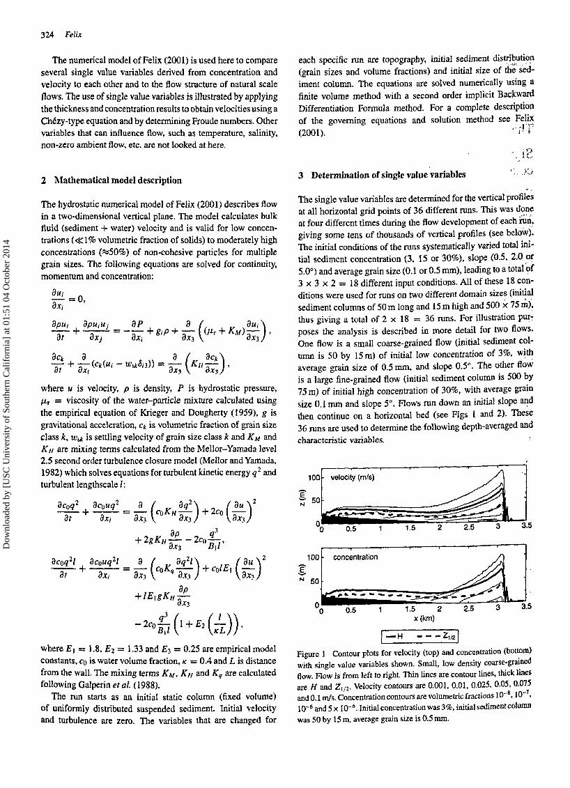
To compare the single value velocities with results of theCMzy-type equation. three velocities were calculated with theChezy-type equation of von Karman and Benjamin using threedifferent sets of single value variables. The depth-averaged con­centration C and thickness H were used to calculate a velocityUda. the characteristic values Ca and Zrnax at the height of thevelocity maximum were used to calculate Urn and the values CI/2and 2 1/2 were used to calculate U 1/2. These three sets ofvariablescan be taken to characterize the flow. The eMzy velocities arecompared to U and Urnax • determined for the two flows shownearlier. The results in Fig. 5 show that Uda and U 1/2 are ofcompa­rable magnitude but Urn is smaller than either. The similarity ofUda and U I /2 indicates that most of the momentum and sedimenttransport of the flow is in the part of the flow below 2 1/ 2, and theupper part does not contribute significantly to the flow dynamics.Porthe fine-grained flow, Uda and UI/2 have values between U andUmax while Urn is lower than either. For the coarse-grained flowthis is only true in the nose of the flow, while for the rest of the flowthe CMzy velocities are smaller than U and Urnax . The differencebetween these results is caused by the different rate of changeof the flows. The fine-grained flow varies slowly and can thusbe described reasonably well by Chezy-type equations but thecoarse-grained flow cannot; only the nose of the coarse-grainedflow changes slowly while the flow structure of the body changesrapidly. None ofthe equations recovers either the depth-averagedvelocity or the velocity at the height for which the concentra­tion and thickness values were used, and the CMzy velocitiesdo not follow the same trends as the velocities to which they arecompared. The CMzy-type equation thus only gives an order ofmagnitude velocity for the part of the flow that changes slowly,but cannot characterize the velocity for the flow as a whole.

7 Froude numbers

The single value variables were also used to calculate densiomej~ric Froude numbers

UFr=--

"fiih'

where the single value variables are used for u. g' and h. A~for the Chezy-type equations, the three different sets of s~ricg~:

value variables were used to obtain three different Proude nu~:bers. shown in Pig. 6. The Proude numbers differ Significan~~~for the different sets of values used. The Froude number Frma:cusing the values at the height of the velocity maximum i~~i:;cates that the bottom part of both flows is supercritical. In ~~

fine-grained flow. the Froude number Frl/2 calculated using ,t?,~

values at 21/2 indicates that the flow goes from being SuP~!;

critical in the tail to (sub)critical towards the nose. The s~;is shown by Frda calculated using the depth-averaged valu~s.~

The transition from supercritical towards (sub)critical is shown. "even more strongly for the coarse-grained flow. The densJomet~

ric Froude numbers in the tail of this flow are very high a~ aresult of the negligible concentration. The transition fro~sulr

critical to supercritical from the nose of the flow to the tail o,fthe flow shows that the interpretation of these Froude numberscannot be the same as in open channel flows. The nose of theflow is not a fast thin flow (as indicated by a supercritical num­ber) nor is the tail a thick slow flow (as indicated by a subcritica!Froude number). The combination ofdeposition, velocity changeand thickness change might give a Proude number that indi­cates a change of regime, even when this does not take placein reality.

Similarly, a hydraulic jump for the entire flow cannot beinferred if the Froude number calculated with single value vari­ables goes from > 1 to < 1. This is the case for the fine-grainedflow. which does not go through a hydraulic jump, even though

328 Felix

, 0.15 r-----...-----,------...----,----,----,----,coarse grained flow

fine grained flow2,----.,----.,..---.,..---...----.....----,----,

1.5

~..... 1~

0.5

en 0.1

:E.~ 0.05

O.....~=__'____'____~__.L..___J..___......._ __.I

o 5 10 15 20 25 30 35x (km)

Figure S Velocity calculations using depth-averaged and characteristic values to determine Chezy velocities. The velocities determined from'~emodel results are the depth-averaged velocity U. maximum velocity Um_. and! Um... The velocities calculated from the eMzy-type equation areu~•• Um and U 1/2'

the density of the turbidity current during flow. It is not clearwhich velocity is calculated from a CMzy-type equation: is thisthe maximum velocity, the depth-averaged velocity orsome other'velocity?

To compare the single value velocities with results of theCMzy-type equation. three velocities were calculated with theChezy-type equation of von Karman and Benjamin using threedifferent sets of single value variables. The depth-averaged con­centration C and thickness H were used to calculate a velocityUda. the characteristic values Ca and Zrnax at the height of thevelocity maximum were used to calculate Urn and the values CI/2and 2 1/2 were used to calculate U 1/2. These three sets ofvariablescan be taken to characterize the flow. The eMzy velocities arecompared to U and Urnax • determined for the two flows shownearlier. The results in Fig. 5 show that Uda and U 1/2 are ofcompa­rable magnitude but Urn is smaller than either. The similarity ofUda and U I /2 indicates that most of the momentum and sedimenttransport of the flow is in the part of the flow below 2 1/ 2, and theupper part does not contribute significantly to the flow dynamics.Porthe fine-grained flow, Uda and UI/2 have values between U andUmax while Urn is lower than either. For the coarse-grained flowthis is only true in the nose of the flow, while for the rest of the flowthe CMzy velocities are smaller than U and Urnax . The differencebetween these results is caused by the different rate of changeof the flows. The fine-grained flow varies slowly and can thusbe described reasonably well by Chezy-type equations but thecoarse-grained flow cannot; only the nose of the coarse-grainedflow changes slowly while the flow structure of the body changesrapidly. None ofthe equations recovers either the depth-averagedvelocity or the velocity at the height for which the concentra­tion and thickness values were used, and the CMzy velocitiesdo not follow the same trends as the velocities to which they arecompared. The CMzy-type equation thus only gives an order ofmagnitude velocity for the part of the flow that changes slowly,but cannot characterize the velocity for the flow as a whole.

7 Froude numbers

The single value variables were also used to calculate densiomej~ric Froude numbers

UFr=--

"fiih'

where the single value variables are used for u. g' and h. A~for the Chezy-type equations, the three different sets of s~ricg~:

value variables were used to obtain three different Proude nu~:bers. shown in Pig. 6. The Proude numbers differ Significan~~~for the different sets of values used. The Froude number Frma:cusing the values at the height of the velocity maximum i~~i:;cates that the bottom part of both flows is supercritical. In ~~

fine-grained flow. the Froude number Frl/2 calculated using ,t?,~

values at 21/2 indicates that the flow goes from being SuP~!;

critical in the tail to (sub)critical towards the nose. The s~;is shown by Frda calculated using the depth-averaged valu~s.~

The transition from supercritical towards (sub)critical is shown. "even more strongly for the coarse-grained flow. The densJomet~

ric Froude numbers in the tail of this flow are very high a~ aresult of the negligible concentration. The transition fro~sulr

critical to supercritical from the nose of the flow to the tail o,fthe flow shows that the interpretation of these Froude numberscannot be the same as in open channel flows. The nose of theflow is not a fast thin flow (as indicated by a supercritical num­ber) nor is the tail a thick slow flow (as indicated by a subcritica!Froude number). The combination ofdeposition, velocity changeand thickness change might give a Proude number that indi­cates a change of regime, even when this does not take placein reality.

Similarly, a hydraulic jump for the entire flow cannot beinferred if the Froude number calculated with single value vari­ables goes from > 1 to < 1. This is the case for the fine-grainedflow. which does not go through a hydraulic jump, even though

Dow

nloa

ded

by [

USC

Uni

vers

ity o

f So

uthe

rn C

alif

orni

a] a

t 01:

51 0

4 O

ctob

er 2

014

Single value variables in turbidity currents 329

100

coarse grained flow11. , '.- 50 ~ I I'rU. 'f'.\

"\ ....\:

a -'-.a 0.5 1.5 2 2.5 3 3.5 4

4 fine gra~e~ fIQ\'Y" .3 .,.. . ./ -.., ,.. - "". -' "'". - - .""

U:: 2

- Frda. _. Fr

max_ ~ Fr

l12

O'----.J..-_-J....__-l-.__.l--_----l__-.l-__--L-_----l

a 5 10 15 20 25 30 35 40x (km)

Figure 6 Froude numbers for the coarse-grained flow (top) and fine-grained flow (bottom) calculated using different sets of single value variables.The concentration of the coarse-grained flow is zero near the origin of the flow (see Fig. 1) so densiometric Froude numbers cannot be calculated.

Fig. 6 shows a change from supercritical to subcritical. As canbe seen in Figs 2 and 4, there is no sudden change of thickness,concentration or velocity at the position of the transition of theFroude number Frl/2. This is not to say that flows cannot undergoa hydraulic jump, as Garda (1993) showed experimentally thatthis can take place, but such behaviour cannot be inferred from asimple Froude number approach.

Since turbidity currents have highly variable values of veloc­ity and concentration at different positions in the flow, bothhorizontally and vertically, flow behaviour is different in differentparts of the flow (Felix, 2002). These differences cannot be rep­resented by single value variables. Hence, although single valuevariables might be useful to describe overall flow properties, theycannot describe internal flow structure, and dimensionless num­bers derived from singlevalue variables must be used with cautionto determine flow processes.

8 Conclusions

Single value variables that describe overall flow transport (totalsediment transport and momentum thickness and velocity), cor­respond to actual physical values of the flow structure for partsof turbidity currents that vary little along flow. For rapidly vary­ing parts of the flow, single value variables only describe valuesrelative to a specific position of the flow structure, e.g. ZI/4.

Single value variables all follow similar trends so to a certainextent they can be used interchangeably. The values that indi­cate overall transport properties are similar for depth-averagedvariables and characteristic variables, as shown by H ~ ZI/4,

U ~ 4Umax and C ~ C1/4. The values at the height of the veloc­ity maximum vary too much to be directly compared to the othersingle value variables, but values higher up in the flow vary muchless between flows.

In this regard, for non-dimensionalizing, ZI/2 may be easierto use than H since the former can be more easily determined

as fewer measurement points are required and only the .lowerpart of the profile needs to be measured.. Although the deter­mination of H, U and C uses information from the entire flow,most of the flow momentum and sediment transport is taken upby the part of the flow below ZI/2 so this value characterizesflow behaviour well and can be used to non-dimensionalize thevertical coordinate.

Single value variables are not indicative of the entire flowstructure of turbidity currents. Flow structure is highly vari­able and depends, among other things, on grain-size distribution,which cannot be taken into account using single value variables.Thus single value variables cannot be used in derived propertiessuch as Froude numbers, or in equations such as the Chezy-typeequation to describe flows with highly variable flow structure.

Acknowledgments

Comments of Lawrence Amy, Jeff Peakall and Susan Sturtongreatly improved the clarity and quality ofearlier versions of thispaper.

Notation

e(z) =concentrationC =depth-averaged concentration

Cm = average concentration below Zmax

CI/2 = average concentration below ZI/2

CI/4 =average concentration below ZI/4

H =depth-averaged flow thicknessu(z) = velocity

U =depth-averaged velocityUmax = maximum velocityZmax =height of velocity maximumZI/2 =height above velocity maximum where u = O.5UmaxZI/4 = height above velocity maximum where u = O.25Umax

Single value variables in turbidity currents 329

100

coarse grained flowI I. , ".- 50 ~ I Il rU. .,..\

"\

\;:

a _.-.a .0.5 1.5 2 2.5 3 3.5 4

4 fine g(ajned flQw.... I" .3 .,. . J -." ,- _ "" _. \,,0 ...... - ...

~.~-_._.~."-.

- Frda. _. Frmax_ ~ Fr,12

OL...-_--J..__-J....__-l-..__"--_----l__-.l-__-L.._---'

o 5 10 15 20 25 30 35 40x (km)

Figure 6 Froude numbers for the coarse-grained flow (top) and fine-grained flow (bottom) calculated using different sets of single value variables.The concentration of the coarse-grained flow is zero near the origin of the flow (see Fig. 1) so densiometric Froude numbers cannot be calculated.

Fig. 6 shows a change from supercritical to subcritical. As canbe seen in Figs 2 and 4, there is no sudden change of thickness,concentration or velocity at the position of the transition of theFroude number Frl/2. This is not to say that flows cannot undergoa hydraulic jump, as Garda (1993) showed experimentally thatthis can take place, but such behaviour cannot be inferred from asimple Froude number approach.

Since turbidity currents have highly variable values of veloc­ity and concentration at different positions in the flow, bothhorizontally and vertically, flow behaviour is different in differentparts of the flow (Felix, 2002). These differences cannot be rep­resented by single value variables. Hence, although single valuevariables might be useful to describe overall flow properties, theycannot describe internal flow structure, and dimensionless num­bers derived from singlevalue variables must be used with cautionto determine flow processes.

8 Conclusions

Single value variables that describe overall flow transport (totalsediment transport and momentum thickness and velocity), cor­respond to actual physical values of the flow structure for partsof turbidity currents that vary little along flow. For rapidly vary­ing parts of the flow, single value variables only describe valuesrelative to a specific position of the flow structure, e.g. ZI/4.

Single value variables all follow similar trends so to a certainextent they can be used interchangeably. The values that indi­cate overall transport properties are similar for depth-averagedvariables and characteristic variables, as shown by H ~ ZI/4,

U ~ 4Umax and C ~ C1/4. The values at the height of the veloc­ity maximum vary too much to be directly compared to the othersingle value variables, but values higher up in the flow vary muchless between flows.

In this regard, for non-dimensionalizing, ZI/2 may be easierto use than H since the former can be more easily determined

as fewer measurement points are required and only the .lowerpart of the profile needs to be measured.. Although the deter­mination of H, U and C uses information from the entire flow,most of the flow momentum and sediment transport is taken upby the part of the flow below ZI/2 so this value characterizesflow behaviour well and can be used to non-dimensionalize thevertical coordinate.

Single value variables are not indicative of the entire flowstructure of turbidity currents. Flow structure is highly vari­able and depends. among other things, on grain-size distribution,which cannot be taken into account using single value variables.Thus single value variables cannot be used in derived propertiessuch as Froude numbers. or in equations such as the ebezy-typeequation to describe flows with highly variable flow structure.

Acknowledgments

Comments of Lawrence Amy, Jeff Peakall and Susan Sturtongreatly improved the clarity and quality ofearlier versions of thispaper.

Notation

e(z) =concentrationC =depth-averaged concentration

Cm = average concentration below Zmax

Cl/2 = average concentration below ZI/2

C'/4 =average concentration below ZI/4

H =depth-averaged flow thicknessu(z) = velocity

U =depth-averaged velocityUmax = maximum velocityZmax =height of velocity maximumZI/2 =height above velocity maximum where u = O.5Umax

ZI/4 = height above velocity maximum where u = O.25Umax

Dow

nloa

ded

by [

USC

Uni

vers

ity o

f So

uthe

rn C

alif

orni

a] a

t 01:

51 0

4 O

ctob

er 2

014

330 Felix

References

1. ALTINAKAR, M.S., GRAF, W.H. and HopfiNGER, E.l. (1996).

"Flow Structure in Thrbidity Currents". J. Hydraul. Res.34(5), 713-718.

2. BENJAMIN, T.B. (1968). "Gravity Currents and RelatedPhenomena". J. Fluid Mech. 31(2),209-248.

3. BUCKEE. C.M. (2000). "Mean Flow and Turbulence Struc­ture in Experimental Gravity Currents". PhD Thesis,University of Leeds, UK, 214 ppo

4. BUCKEE, C., KNELLER, B. and PEAKALL, J. (2001). ''Thrbu­lence Structure in Steady, Solute-Driven Gravity Currents".In: MCCAfFREY, W.D., KNELLER, B.C. and PEAKALL, J.(eds), Particulate Gravity Currents. lAS Spec. Publ., 31,pp.173-187.

5. DALY, R.A. (1936). "Origin of Submarine Canyons".Am. J. Sci. 31(186),401-420.

6. EWSON, T.H. and TURNER, ].S. (1959). "Turbulent Entrain­ment in Stratified Flows". J. Fluid Mech. 6, 423-448.

7. FELIX, M. (2001). "A 1\vcrDimensional NumericalModel for a Turbidity Current... · In: MCCAFFREY, W.D.,KNELLER, B.C. and PEAKALL, J. (eds), Particulate GravityCurrents. lAS Spec. Pub!., 31, pp. 71-81.

8. FELIX, M. (2002). "Flow Structure of Turbidity Currents".Sedimentology 49,397-419.

9. GALPERlN, Bo, KANTHA, L.H... HASSID, S. and ROSATI, A.(1988). " A Quasi-Equilibrium Thrbulent Energy Model forGeophysical Flows". J. Atm. Sci. 450), 55~2.

10. GARCIA, M.H. (1993). "Hydraulic Jumps in Sediment­Driven Bottom Currents". J. Hydraulo Engng. 119(10),1094-1117.

11. GARdA, M.H. (1994). "Depositional Thrbidity CurrentsLaden with Poorly Sorted Sediment". J. Hydraul. Engng.120(11),1240-1263.

12. KNELLER, B.C., BENNETT, SJ. and MCCAfFREY, WD.(1999). "Velocity Structure, Turbulence and Fluid Stressesin Experimental Gravity Currents". J. Geophys. Res.104(C3),5381-5391.

13. KRIEGER, I.M. and DOUGHERTY, TJ. (1959). "A Mechanismfor Non-Newtonian Flow in Suspension of Rigid Spheres".Trans. Soc. Rheol. 3, 137-152.

14. KUENEN, Ph.H. (1937). "Experiments in Connectionwith Daly's Hypothesis on the Formation of SubmarineCanyons". I..eidsche Geol. Meded. VIII(2), 327-351.

15. KUENEN, Ph.H. (1952). "Estimated Size of the Grand BanksTurbidity Current". Am. J. Sci. 250(12),874-884.

16. LEE, H.-Y. and Yu, W-S. (1997). "Experimental Study ofReservoir Thrbidity Current". J. Hydraul. Engng. 123(6),

520-528.17. MELLOR, G.L. and YAMADA, T. (1982). "Develop­

ment of a Thrbulence Closure Model for GeophysicalFluid Problems". Rev. Geophys. Space Phys. 20(4),851-875. ..

18. MIDDLETON, G.V. (1966). "Experiments on Density andTurbidity Currents. I. Motion of the Head". Can. J. EarthSci. 3(4),523-546.

19. PARKER, G., fuKUSHIMA, Y. and PANTIN, H.M. (1986)."Self-Accelerating Thrbidity Currents". J. Fluid Mech. 171,

145-181.20. VON KARMAN, T. (1940). "The Engineer Grapples

with Nonlinear Problems". Bull. Am. Math. Soc. 46,615-683.

330 Felix

References

1. ALTINAKAR, M.S., GRAF, W.H. and HopfiNGER, E.J. (1996).

"Flow Structure in Thrbidity Currents". J. Hydraul. Res.34(5),713-718.

2. BENJAMIN, T.B. (1968). "Gravity Currents and RelatedPhenomena". J. Fluid Mech. 31(2),209-248.

3. BUCKEE, C.M. (2000). "Mean Flow and Thrbulence Struc­ture in Experimental Gravity Currents". PhD Thesis,University of Leeds, UK, 214 pp,

4. BUCKEE, C., KNELLER, B. and PEAKALL, J. (2001). ''Turbu­lence Structure in Steady, Solute-Driven Gravity Currents".In: MCCAFFREY, W,O., KNELLER, B.C. and PEAKALL, J.(eds), Particulate Gravity Currents. lAS Spec. Publ., 31,pp.173-187.

5. DALY, R.A. (1936). "Origin of Submarine Canyons".Am. J. Sci. 31(186),401-420.

6. EWSON, T.H. and TURNER, J.S. (1959). "Thrbulent Entrain­ment in Stratified Flows", J. Fluid Mech, 6, 423-448.

7. FELIX, M. (2001). "A Two-Oimensional NumericalModel for a Thrbidity Current".' In: MCCAFFREY, W.O.,KNELLER, B.C. and PEAKALL, 1. (cds), Particulate GravityCurrents. lAS Spec. Pub!., 31, pp. 71-81.

8. FELIX, M. (2002). "Flow Structure of Thrbidity Currents".Sedimentology 49,397-419.

9. GALPERIN, B., KANTHA. L.H. .. HASSID, S. and ROSATI, A.(1988)... A Quasi-Equilibrium Thrbulent Energy Model forGeophysical Flows". J. Atm. Sci. 45(1), 55-62.

10. GARCIA, M.H. (1993). "Hydraulic lumps in Sediment­Driven Bottom Currents". J. Hydraul, Engng. 119(10),1094-1117.

11. GARCIA, M.H. (1994). "Depositional Thrbidity CurrentsLaden with Poorly Sorted Sediment". J. Hydraul. Engng.120(11),1240-1263.

12. KNELLER, B.C., BENNETT, S.J. and McCAfFREY, WO.(1999). "Velocity Structure, Turbulence and Fluid Stressesin Experimental Gravity Currents". J. Geophys. Res.104(C3),5381-5391.

13. KRIEGER, I.M. and DOUGHERTY, T.1. (1959). "A Mechanismfor Non-Newtonian Flow in Suspension of Rigid Spheres".

Trans. Soc. Rheol. 3, 137-152.14. KUENEN, Ph.H. (1937). "Experiments in Connection

with Daly's Hypothesis on the Formation of SubmarineCanyons". uidsche Geol. Meded. VIII(2), 327-351.

15. KUENEN, Ph.H. (1952). "Estimated Size of the Grand BanksTurbidity Current". Am. J. Sci. 250(12),874-884.

16. LEE, H.-Y. and YU. W-S. (1997). "Experimental Study ofReservoir Thrbidity Current", J. Hydraul. Engng. 123(6).

520-528.17. MELLOR, G.L. and YAMADA, T. (1982). "Develop­

ment of a Turbulence Closure Model for GeophysicalFluid Problems". Rev. Geophys. Space Phys. 20(4),

851-875.'18. MIDDLETON, G.V. (1966). "Experiments on Density and

Turbidity Currents. I. Motion of the Head". Can. J. EarthSci. 3(4),523-546.

19. PARKER, G., fuKUSHIMA, Y. and PANTIN. H.M. (1986)."Self-Accelerating Thrbidity Currents". J. Fluid Mech. 171,

145-181.20. VON KARMAN, T. (1940). "'The Engineer Grapples

with Nonlinear Problems". Bull. Am. Math. Soc. 46,615-683.

Dow

nloa

ded

by [

USC

Uni

vers

ity o

f So

uthe

rn C

alif

orni

a] a

t 01:

51 0

4 O

ctob

er 2

014