The Short and Long-Run Financial Impact of Corporate

The Short and Long-Run Financial Impact of Corporate Outsourcing Transactions

University of Pittsburgh

2006

Submitted to the Graduate Faculty of

Joseph M. Katz Graduate School of Business in partial fulfillment

of the requirements for the degree of

Doctor of Philosophy

by

Ning Gao

B.A. in Accounting, Ren Min University, 1998

M.A. in Economics, Florida State University, 2001

ii

UNIVERSITY OF PITTSBURGH

Joseph M. Katz Graduate School of Business

This dissertation was presented

by

Ning Gao

It was defended on

July 25, 2006

and approved by

Steven Husted, PhD, Professor

Frederik Schlingemann, PhD, Associate Professor

Shawn Thomas, PhD, Associate Professor

Chad Zutter, PhD, Assistant Professor

Dissertation Advisor: Kuldeep Shastri, PhD, Professor

iii

Copyright © by Ning Gao

2006

iv

This dissertation investigates the financial impact of a large sample of outsourcing contracts

signed by corporations listed on the US markets from 1990 through 2003. We construct a data

set that identifies the outsourcing client and vendor firms and use this data set to examine (a) the

announcement effects of outsourcing contracts on firm value, (b) the impact of outsourcing

contracts on long-run stock and accounting performance and (c) the impact of outsourcing

contracts on the relation between client and vendor firms.

The Short and Long-Run Financial Impact of Corporate Outsourcing Transactions

Ning Gao, PhD

University of Pittsburgh, 2006

v

TABLE OF CONTENTS

1.0 INTRODUCTION........................................................................................................ 1

2.0 A REVIEW OF THE LITERATURE........................................................................ 5

3.0 THE TESTABLE HYPOTHESES ........................................................................... 10

3.1 THE SHORT-RUN FINANCIAL IMPACT OF THE ANNOUNCEMENT

OF OUTSOURCING TRANSACTIONS......................................................................... 10

3.1.1 Information Asymmetry............................................................................. 10

3.1.2 Economies of scale....................................................................................... 10

3.1.3 Focus on core competency.......................................................................... 11

3.1.4 Flexibility ..................................................................................................... 11

3.1.5 Contract Size ............................................................................................... 12

3.1.6 Country of origin......................................................................................... 12

3.2 THE LONG-RUN FINANCIAL IMPACT OF THE SIGNING OF

OUTSOURCING TRANSACTIONS ............................................................................... 13

3.3 OUTSOURCING TRANSACTIONS AS STRATEGIC

ALLIANCES/PARTNERSHIPS....................................................................................... 13

4.0 THE METHODOLOGY ........................................................................................... 14

4.1 ESTIMATING THE SHORT-RUN IMPACT OF THE ANNOUNCEMENT

OF OUTSOURCING TRANSACTIONS......................................................................... 14

4.1.1 Estimating Abnormal Returns and Test Statistics .................................. 14

4.1.2 Cross-Sectional Tests .................................................................................. 16

4.2 ESTIMATING THE LONG-RUN IMPACT OF THE SIGNING OF


4.2.1 Calculating long-run buy-and-hold stock returns ................................... 18

4.2.2 Measuring changes in accounting performance....................................... 20

vi

4.2.3 Measuring Abnormal Returns in Calendar Time.................................... 21

4.3 MEASURING THE IMPACT OF OUTSOURCING TRANSACTIONS

WHEN VIEWED AS STRATEGIC ALLIANCES/PARTNERSHIPS......................... 22

4.3.1 Measuring the Relation between Client and Vendor Stock Prices......... 22

4.3.2 Measuring Correlations in Accounting Performance ............................. 24

5.0 THE SAMPLE AND DATA...................................................................................... 26

5.1 THE SAMPLE ................................................................................................... 26

5.2 A DESCRIPTION OF THE DATA ................................................................. 27

6.0 EMPIRICAL RESULTS ........................................................................................... 29

6.1 SHORT-RUN IMPACT OF THE ANNOUNCEMENT OF


6.1.1 Univariate results ........................................................................................ 29

6.1.2 Multivariate results..................................................................................... 33

6.2 THE LONG-RUN IMPACT OF THE SIGNING OF OUTSOURCING

TRANSACTIONS .............................................................................................................. 35

6.2.1 Long-Run Stock Returns for Client Firms after the Signing of

Outsourcing Transactions ......................................................................................... 35

6.2.2 Long-Run Accounting Performance of Client Firms after the Signing of

Outsourcing Transactions ......................................................................................... 37

6.3 THE LONG-RUN INTEGRATION OF THE CLIENT AND VENDOR

FIRMS 39

6.3.1 The Relation between Client and Vendor Stock Returns in the Pre and

Post-Signing Period.................................................................................................... 40

6.3.2 The Relation between Client and Vendor Accounting Performance in

the Pre and Post-Signing Period ............................................................................... 42

7.0 CONCLUSIONS ........................................................................................................ 43

REFERENCE.............................................................................................................................. 45

vii

LIST OF FIGURES

Figure 1. Frequency of outsourcing deals..................................................................................... 47

Figure 2. Value of outsourcing deals ............................................................................................ 47

viii

LIST OF TABLES

Table 1. Descriptive Statistics for Signed Contracts, Client and Vendor Firms........................... 48

Table 2. Descriptive Statistics for Cancelled Contracts................................................................ 50

Table 3: Abnormal returns for client firms around outsourcing contract announcements ........... 51

Table 4: Abnormal returns for vendors around outsourcing contract announcements................. 58

Table 5: The relation between client firms’ announcement day abnormal stock returns and

measures of firm and contracts’ characteristics ............................................................................ 63

Table 6: The relation between vendors’ announcement day abnormal stock returns and measures

of firm and contracts’ characteristics............................................................................................ 65

Table 7: Ex-post long-run holding period abnormal returns for client firms................................ 66

Table 8: Ex-ante holding-period abnormal returns for client firms.............................................. 69

Table 9: Calendar-time three-factor model for client firms.......................................................... 70

Table 10: Regressions of client firms’ long-run abnormal stock returns...................................... 71

Table 11: Ex-post long-run holding period abnormal returns of vendor firms............................. 72

Table 12: Ex-post accounting performance changes for client firms ........................................... 73

Table 13: Ex-ante accounting performance changes of client firms............................................. 83

Table 14: Regressions of client firms’ long-run accounting performance changes...................... 84

Table 15: Ex-post accounting performance changes of vendor firms........................................... 85

Table 16: Regressions of vendor firms’ long-run abnormal stock returns and accounting

performance changes .................................................................................................................... 86

Table 17: The changes in daily stock return cross-correlations between client and vendor firms87

Table 18: Cross-sectional regression of daily returns cross-correlation changes ......................... 88

Table 19: Long-run buy-and-hold stock return cross-correlations between client and vendor firms

....................................................................................................................................................... 90

ix

Table 20: Granger causality tests.................................................................................................. 91

Table 21: Unadjusted accounting performance change cross-autocorrelation test....................... 92

Table 22: Industry-median adjusted accounting performance change cross-autocorrelation tests93

Table 23: Cross-autocorrelations of percentage changes in return on assets................................ 94

1

1.0 INTRODUCTION

Outsourcing defined as the delegation of non-core operations from internal production within a

firm (client firm) to an external entity that specializes in that operation (vendor firm) became a

popular buzzword in business in the mid 1990s. Although outsourcing has been a management

practice for over 200 years it has received more attention in the recent past since the volume of

international outsourcing has grown rapidly.1 Proponents of outsourcing argue that this activity

helps client firms by providing them with the ability to (i) purchase intellectual capital that may

otherwise not be available to them, (ii) focus more on core competencies, (iii) better anticipate

future costs and (iv) lower costs. This implies that outsourcing helps US firms become more

profitable, thereby benefiting shareholders.2 Opponents of international outsourcing argue that

this activity hurts the economy of the United States of America, reduces the quality of service

provided and jeopardizes security. For example, in the 2004 presidential campaign, Democratic

candidate John Kerry claimed that international outsourcing was a major cause of unemployment

in the US and blasted companies and Chief Executive Officers (CEOs) that outsource calling

them “Benedict Arnold Corporations and CEOs” and argued for intervention by the US

government. This view seems to be shared by the American public since a Zoghy International

poll in 2004 reported that 71 percent of those polled believed that outsourcing jobs overseas

hurts the US economy and 62 percent think that the government should impose legislative

restrictions on outsourcing. In contrast, a Wall Street Journal poll of economists reports that only

16 percent of those surveyed saw outsourcing as having a significant impact on jobs. As a matter

of fact, many suggested that outsourced jobs are replaced by better paying jobs in another

1 For example, there was not much publicity when Eastman Kodak Company contracted away the management of its data centers to IBM Corporation in 1989 or when American Express set up its back-office operation in India more than a decade ago. 2 For example, on December 9, 2002 when Anthem Inc. signed an information technology (IT) outsourcing contract with Affiliated Computer Services, Inc., the stock of Anthem Inc, displayed a market-adjusted abnormal return of 1.14 percent.

2

area/industry and that outsourcing is just a new way of doing international trade. For example,

Drezner (2004) reports that although 70,000 computer programmers lost their jobs between 1999

and 2003, 115,000 computer software engineers found higher paying jobs within the same

period. In addition, the McKinsey Global Institute has estimated that for every dollar spent on

outsourcing to India, the US reaps between $1.12 and $1.14 in benefits.

As stated previously, outsourcing has been part of business practice for many years but

has garnered much more attention recently because of both the historical and forecasted growth

in the number and volume of these transactions. Figures 1 and 2 provide a historical perspective

on the annual number and total value of outsourcing transactions signed by firms with stocks

listed in the US over the period starting in January 1990 and ending in December 2003. As can

be seen from these figures, the number of outsourcing deals per year has grown from 7 in 1990

to 216 in 2003 with a peak of 241 in 2002. The corresponding figures for the total value of

outsourcing deals signed per year (in 2000 dollars) are $226.25 million, $27.78 billion and

$61.98 billion (in 2002), respectively.3 Deavers (1997) argues that this increase in outsourcing

activities is a result of rapid technological change, increased risk and the search for flexibility,

greater emphasis on core competencies and globalization.

In terms of future growth, the McKinsey Global Institute estimates that the size of this

market is going to grow at a rate between 30 and 40 percent per year for the next five years. In

addition, a recent report by the business consultant company INPUT states that outsourcing

expenditures on the Information Technology (IT) sector alone is expected to grow from $10

billion in fiscal year 2005 to approximately $18 billion in fiscal year 2010.

Given the magnitude of the market for these transactions and the controversy surrounding

offshore outsourcing, a natural question that arises is as follows: what is the magnitude of the

benefits of outsourcing to the client and vendor firms and what are its determinants? The

purpose of this paper is to examine the short and long-run financial impact of outsourcing

transactions on client and vendor firms over the 1990 to 2003 period. Specifically, we first

analyze the impact of announcements of outsourcing contracts on the stock prices of the client

and vendor firms and provide an examination of the cross-sectional determinants of the

announcement effect. Second, we study the impact of outsourcing contracts on the long-run

3 The numbers reported in Figures 1 and 2 are based on the outsourcing sample used in this study. See Section 5 for more details on our sample.

3

accounting and stock performance of the client firms. Third, we analyze the impact of

outsourcing contracts on the relation between the long-run accounting and stock performance of

the client and vendor firms.

Our results indicate that the average abnormal return for client firms on the

announcement day of outsourcing contracts (day 0) is an insignificant 0.145 percent. On the

other hand, multivariate tests indicate that the announcement is associated with positive day 0

abnormal returns. Specifically, we find that the abnormal return decrease with client firm size

and client firm flexibility while they increase with the relative size of the vendor firm to the

client firm and client firm opacity. Based on these results, we conclude that the short-run of

outsourcing transactions can be partially attributed information asymmetry. In addition, our

results are consistent with the hypothesis that outsourcing is undertaken to take advantage of

economies of scale, to have the ability to focus more on core competencies and to provide more

operating flexibility.

We also find that the rivals of the client firms experience a negative day 0 abnormal

return. This suggests that in the eyes of the market, signing the outsourcing contract provides the

client firm with competitive advantages vis-à-vis the rest of the industry.

With respect to vendor firms we find that they gain 1.303 percent on the announcement

day. This gain decreases with vendor size and increases with the size of the deal. We also find

those deals that are renewals of previously signed deals have a smaller impact on day 0 stock

prices. Overall this suggests support for hypothesis that the short-term effect of the

announcements of outsourcing transactions on vendor firms are partially driven by information

asymmetry. In addition, the results also indicate support for the hypotheses that the sources of

gains to vendor firms from outsourcing are economies of scale and the amount the contract

enhances the vendor’s revenue stream.

We also find that the rivals of vendor firms experience a positive abnormal return on day

0. This result is consistent with the good news associated with the announcement having a

contagion effect in the industry.

Given that vendors experience a positive abnormal return when it is learned that they

have been awarded an outsourcing contract, one would expect the opposite on an announcement

of a contract being cancelled by the client firm or when the client firm announces that the vendor

was not chosen to be the partner in a particular transaction. Our results are consistent with this

4

hypothesis. Specifically, we find that vendors experience a negative day 0 abnormal return

around such announcements.

In the case of client firms, long-run stock and accounting performance is consistent with

the results reported above for short-run stock performance. Specifically, we find that the buy-

and-hold returns (BHARs) for client firm stocks in the 3-year period prior to the outsourcing

transaction are not significantly different from the BHARs for a control group of firms. On the

other hand, BHARs for client firms in the post-outsourcing period are significantly larger than

that for the control group. The same result hold for measures of accounting performance

including sales per employee, income per employee, gross profit margin, net profit margin, and

asset turnover.

Finally our results are consistent with the view that outsourcing transactions create a

strategic partnership between client and vendor firms. Specifically we find that client and vendor

firm stock returns are not correlated prior to outsourcing transactions but the correlation becomes

significantly positive in the post-outsourcing period. The same result holds true for changes in

accounting performance when accounting performance is measured by return on assets and asset

turnover.

The remainder of this dissertation is organized as follows. Section 2 reviews the literature

of the financial impact of outsourcing. Section 3 identifies the specific hypotheses that are tested

here. Section 4 describes the methodology used in the tests of the hypotheses, while Section 5

contains a description of the sample and data. The empirical results and the interpretation of the

results are contained in Section 6 and Section 7 concludes.

5

2.0 A REVIEW OF THE LITERATURE

The early outsourcing literature employs the “economics of transaction cost” model of the firm

as the primary theoretical lens to examine outsourcing arrangements. 4 According to Coase

(1937), the limits of the firm are determined by the relative production costs inside the firm as

compared with the costs of using the market (outsourcing). Williamson (1985) attributes

transactions costs to supplier hold-ups after customers have already invested in relationship

specific assets. Thus, when hold-up problems are very costly, internal hierarchies are more

advantageous to external relationships (outsourcing).

Grossman and Helpman (2002) theoretically examine a firm’s decision to produce in-

house or outsource. They model the “make or buy” decision as a trade-off between diseconomies

of scope and the transaction costs that stem from search frictions and incomplete contracts. They

find that where the cost advantage of specialized component producers is large and their

bargaining power vis-à-vis specialized final producers is great, outsourcing is more likely to

emerge in a stable equilibrium the greater is the substitutability between varieties of final goods.

The transaction cost theory of the firm suggests that as firms evolve and compare the

costs of an internal versus external hierarchy, they will engage in outsourcing as they start to

recognize that the production costs of managing their own internal operations may be reduced by

outsourcing due to the effect of considerable economies of scale.5 Specifically, by outsourcing,

client firms can benefit from economies of scale when there are large specialist vendor firms that

can provide the services at lower average cost..

Another possible reason for firms recognizing the value of outsourcing could be a result

of an external shock to their operating environment. For example, Sharpe (1997) suggests that

4 For more details on the theory of the firm based on the economics of transactions costs, see Coase (1937) and Williamson (1979). 5 For example, see Abraham and Taylor (1996), Sharpe (1997), Deavers (1997) and McCarthy and Anagnostou (2004).

6

deregulation of telecommunications companies in the 1980s and public utility companies in the

1990s caused a change in the operating environment of these companies resulting in their

embracing outsourcing as a more efficient way of doing business. Specifically, Sharpe states that

“outsourcing did not emerge as the consequence of a sudden technical breakthrough, nor did it

grow out of a best selling book by a well-known management guru. Rather, it was the result of

market forces that emerged in response to demands for more efficient ways to address

organizational competitiveness.”

Quinn and Hilmer (1994) make a core competency argument for the use of outsourcing.

Specifically, they suggest that the potential gains offered by outsourcing are optimized when

outsourcing enhances a “core competency” business strategy. Thus, when correctly or optimally

combined, core competency and extensive outsourcing strategies provide more flexibility,

greater efficiency and better responsiveness to customer needs at lower costs. Most importantly,

they suggest that strategic outsourcing provides organizations with a competitive edge in the

long run.

There is anecdotal evidence that corporate decision makers act in a way consistent with

this strategic outsourcing theory. For example, at the time of signing a five-year outsourcing

contract worth $2.1 billion in July 1991 by LaBarge Inc. and McDonnell Douglas Co., William

Maender, LaBarge’s vice president, said that “it is an effort to improve operating efficiency,

control costs, standardize practices among plants and comply with the demanding government

reporting requirements of manufacturing for the defense market.” In another example when

Affiliated Computer Services Inc. (ACS) announced the renewal of a comprehensive IT

outsourcing agreement with Affiliated Health Services of Mt. Vernon, Washington in January

2000, Tom Litaker, CFO of Affiliated Health Services said that "ACS has the experience and

expertise to integrate technology with our business and help us reach our goals in the future. We

expect ACS' broad range of services and industry knowledge to bring us efficiency and cost

effectiveness in operations as we focus on providing the best possible care to our constituents."

In summary, the rationale for firms to outsource is that this activity helps organizations

increase operating efficiency, reduce operating costs, while achieving an increased focus on core

competencies. This would suggest that client and vendor firms should benefit in the short-run

and long-run from signing these outsourcing contracts.

7

There are a few studies that have examined the short-run stock price impact of

outsourcing transactions. One of the earliest papers is one by Hayes, Hunton and Reck (2000) in

which they analyze the effect of the announcement to outsource all or a portion of a firm’s

information systems (IS) functions on the market value of the client firm. The first hypothesis

they test is that IS outsourcing announcements will have a greater positive impact on the market

value of smaller firms as compared to the market value of larger firms, because there tends to be

more information asymmetry about smaller firms. Specifically, announcements made by small

firms are expected to yield a greater market response because of the bigger surprise they

generate. Second, they hypothesize that the impact of IS outsourcing announcements would have

a greater positive impact on the market values of service firms as compared to the market values

of non-service firms. This hypothesis is based on the argument that there is more information

asymmetry about service firms since standard financial-reporting systems do not capture many

factors (such as intellectual capital and other “soft” assets) important to service industries and

that service firms allocate a higher proportion of their resources to information technology as

compared to non-service firms. This implies that the reaction to the announcement should be

more positive because it is more of a surprise and is more meaningful to the firm.

Using a sample of client firms that announce IS outsourcing arrangements from 1990

through 1997, they find no statistically significant stock price change for a two-day event

window for their complete sample of client firms.6 For their sub-sample of small firms, they

report weakly significant positive abnormal stock returns for the two-day event window. For a

one-day window (the day after the announcement day), they report significant positive abnormal

stock returns for both small firms and service firms. Finally, they find support for both their

hypotheses in a multivariate regression analysis.

There are several other papers that follow Hayes et. al. (2000) and employ the event

study methodology to examine the short-run impact of the announcement of outsourcing

transactions. For example, Farag and Krishnan (2003) examine IT outsourcing deals announced

between January 1994 and August 2001 and find that there are positive announcement effects for

outsourcing decisions by firms in the IT and service industries. They also find that the stock

price react positively to the announcement of strategic sourcing projects but not to cost cutting

projects. Gellrich and Gewald (2005) examine outsourcing decisions by firms in the financial

6 The two-day event window consists of the announcement day and the day after the announcement day.

8

services industry and find that there are positive announcement effects associated with large

deals, deals that involve experienced vendors and those that involve the IT function.

There is a paucity of empirical evidence on the long-run effects of outsourcing

transactions. One exception is Gilma and Görg (2004) who examine the impact of outsourcing

decisions by UK manufacturing firms on the labor productivity. They find that outsourcing is

associated with improved labor productivity in the long-run.

A majority of the empirical literature on outsourcing focused on only one party in the

contract, that is, either the client or vendor firm. In contrast, on the theoretical level the literature

recognized outsourcing transactions as a project assigned by the client firm (the principal) to the

vendor firm (the agent). This could lead to potential agency problems since the two parties do

not have perfectly matched goal.7 These agency issues can be mitigated by developing contracts

between the two parties that specify the relationship between the two parties and define the

performance metrics that can be used by the principal to monitor the agent.8 More recently, it has

been argued in the literature that rather than viewing outsourcing transactions as simple

transactional contracts, they should be viewed as strategic alliances/partnerships between the

client and vendor firms.9 For example, Natovich (2003) uses a case study of a project failure to

argue that a contract-driven approach to mitigate vendor risk in outsourcing transactions may not

be as effective as a partnership approach to sharing risk.10

This strategic alliance view of outsourcing transactions has significant implications for

the future relation between the accounting and stock price performance of the client and vendor

firms. Specifically, one would expect the performance metrics for the two firms to become more

correlated with each other after the signing of the outsourcing transaction.

This dissertation extends the extant finance and IS literature on outsourcing in a number

of ways. First, it provides a more complete picture of the impact of the announcement of the

signing of outsourcing transaction by looking at both the client and vendor firms. Second, it

7 For example, see Banker and Kemerer (1992) 8 For example, see Chaudhury, Nam and Rao (1995). 9 For example, see Gallivan and Oh (1999). 10 The case study in Natovich (2003) is that of an outsourcing contract between a telecommunications company, Bezeq (the client) and a software company, AMS (the vendor) to develop the code for a new billing system that was signed in September 1997. Bezeq cancelled the contract in August 1999 and terminated the project before even a single line of code was delivered.

9

analyzes the long-run impact of outsourcing transactions on client firms, an area not explored

previously. Finally, it provides a direct test of the “strategic alliance” hypothesis.

10

3.0 THE TESTABLE HYPOTHESES

3.1 THE SHORT-RUN FINANCIAL IMPACT OF THE ANNOUNCEMENT OF

OUTSOURCING TRANSACTIONS

The argument presented in the previous section would suggest that the announcement of

outsourcing transactions should be associated with an increase in the client and vendor firms’

stock prices. Again, the previous literature suggests that the magnitude of the stock price increase

should vary across firms based on a number of factors that include firm size, economies of scale

involved, the degree of focus on core competencies, flexibility provided by the outsourcing, the

size of the contract and the location of the vendor firm.

3.1.1 Information Asymmetry

It is well recognized in the literature that the amount of publicly available information is not

equal for firms of different sizes. Since large firms are more closely followed by media and

analysts than small firms one would expect less information asymmetry to be associated with

large firms. This would imply that announcements by smaller firms should be associated with a

larger announcement-day movement in stock price. This suggests that the market reaction of the

client (vendor) firm’s stock to corporate outsourcing announcements will be a decreasing

function of the size of the client (vendor) firm.

3.1.2 Economies of scale

It was argued earlier that outsourcing takes advantage of the economies of scale available

through the vendor firm by saving overall production costs and improving operating efficiency

11

for the client firm. It has also been suggested that larger firms enjoy better economies of scale

than their smaller counterparts.11 Thus, one would expect the market reaction of the client firm’s

stock to corporate outsourcing announcements to be the smallest for contracts between large

clients and small vendors and the largest for contracts between small clients and large vendors.

3.1.3 Focus on core competency

It was argued earlier that by focusing on its core competencies and strategically outsourcing

other activities, a firm can create unique value for their customers and that, in turn, can help the

firm maintain its competitive edge in the long run. Therefore, this increase focus in core

competencies should translate into higher stock values for the client firm.

We use opacity as a measure of the degree to which a firm has focused on core

competencies. Specifically, opacity measures whether a firm’s earnings are more dependent on

the realization of future growth opportunities than on assets already in place. The specific

measure of opacity used here is net plant, property and equipment (PPE) divided by total assets

(PPE/TA) with firms having high values of PPE/TA being considered more transparent and

being more focused on core competencies. This suggests that the market reaction of the client

firm’s stock to corporate outsourcing announcements will be a decreasing function of opacity

(PPE/TA).12

3.1.4 Flexibility

Outsourcing can also help provide greater flexibility, especially in the purchase of rapidly

developing new technologies, fashion goods, or the myriad components of complex systems.13 It

11 For example, see Sharpe (1997). 12 One possible problem with this conclusion is that our measure of opacity may just be a proxy for firms in the business service industry since such firms tend to have a low PPE to total assets ration. To ensure that are results are not driven by this factor, we examine firms that do not belong to the business service industry separately. Our results indicate that firms with low opacity in this group experience a day 0 abnormal return of 1.455 percent with an associated significance level of 10 percent. This suggests that the argument that client firms outsource to focus on core competencies is not driven by firms in the business service industry. 13 For example, see Carlson (1989) and Domberger (1998).

12

allows companies to incorporate the latest technology and respond to changes in business

environment more quickly and at a lower cost than vertically integrated organizations. Flexibility

is measured here by two liquidity ratios - the current ratio and the quick ratio. Specifically, the

higher a firm’s liquidity ratio, the better able they are to meet short-term obligations and the

greater their financial flexibility. Since client firms with low liquidity ratios have less financial

flexibility, we would expect them to benefit more from outsourcing. Therefore, the market

reaction of the client firm’s stock to corporate outsourcing announcements will be decreasing

function of firm liquidity.

3.1.5 Contract Size

It can be argued that a larger contract size represents potentially larger cost savings for the client

firm and a potentially larger revenue stream for the vendor firm. This would suggest that the

market reaction of both the client firm’s and vendor firm’s stocks to outsourcing contract

announcements increases with the size of the contract.

3.1.6 Country of origin

A number of groups have suggested that international outsourcing is not good for the US

economy because it results in a firm substituting higher paying jobs in the US for lower paying

jobs in another country. This would imply that the announcement of international outsourcing

contracts should be associated with a larger market reaction in the client firm’s stock price as

compared to the announcement of domestic outsourcing contracts. On the other hand, it has been

argued that outsourcing of any sort is a response by firms facing a complex change in its cost

boundaries and the choice between domestic and international vendor firms is solely dependent

on which firm provides the best strategic fit.14 In this scenario, the market reaction of both the

client firm’s stock to outsourcing contract announcements should not be dependent on the

country of origin of the vendor.

14 For example, see Deavers (1997)

13

3.2 THE LONG-RUN FINANCIAL IMPACT OF THE SIGNING OF


As stated previously, the second objective of this dissertation is to examine the impact of

outsourcing transactions on the long-run performance of the client firms. In the previous section

we argued that the announcement of outsourcing transactions should be associated with an

increase in the client firm’s stock price. This hypothesized increase in stock price results from an

expectation in the market that the client firm will be operating more efficiently in the future.

Thus one would expect that client firms would exhibit abnormally positive long-run accounting

and stock price performance. In addition, since the impact of outsourcing is hypothesized to be

more positive for smaller, more opaque and less flexible client firms, we would expect the same

to be true with long-run abnormal performance.

3.3 OUTSOURCING TRANSACTIONS AS STRATEGIC

ALLIANCES/PARTNERSHIPS

As stated earlier, it has been argued in the literature that rather than viewing outsourcing

transactions as simple transactional contracts, they should be viewed as strategic

alliances/partnerships between the client and vendor firms. This strategic alliance view of

outsourcing transactions has significant implications for the future relation between the

accounting and stock price performance of the client and vendor firms. Specifically, one would

expect the performance metrics for the two firms to become more correlated with each other

after the signing of the outsourcing transaction.

14

4.0 THE METHODOLOGY

4.1 ESTIMATING THE SHORT-RUN IMPACT OF THE ANNOUNCEMENT OF


4.1.1 Estimating Abnormal Returns and Test Statistics

We estimate the short-run impact of the announcement of outsourcing transactions using the

methodology outlined in Brown and Warner (1985) to calculate abnormal returns on stocks

around a day of interest. Specifically, for all the outsourcing deals in our sample, we define the

contract announcement day as event day zero. 15 A trading date that is t days before the

announcement day is denoted as day –t, while a trading day t days after the announcement is

denoted as day +t. The analysis is based on stock returns over a period starting at day -250 and

ending at day +10 (-250, +10). The first 240 days in this period (-250, -11) are designated as the

“estimation period”, and the following 21 days (-10, +10) are designated as the “announcement

period”. The “market model” is used to adjust for market-wide risk factors. Specifically, for any

security j , the abnormal or excess return over each of the t=-10, ...,10 days around the time of

the contract announcement is defined as,

)ˆˆ( mtjjjtjt RRA βα +−= (1)

where jtA is the abnormal return for security j at event day t , Rjt is return on security j at

event day t and Rmt is return on Center for Research in Security Price (CRSP) value-weighted

index at event day t . The coefficients $α j and

$β j are Ordinary Least Squares (OLS) estimates

15 A description of our sample and the methods used to identify the announcement date are provided in Section 5.

15

from the regression of the return on security j on the CRSP value-weighted index over the

estimation period.

The statistical significance of the abnormal returns is assessed in two ways depending on

whether the returns under consideration are one event day or multiple event days in the

announcement period. For a single event day, the t statistic is calculated as the ratio of that event

day’s mean excess return to its estimated standard deviation. Specifically, let tN represent the

number of sample securities whose excess returns are available on event day t . Then we can

express the test statistic for any single event day t as,

)(ˆ/ tt ASA (2)

where

∑=

=tN

jjt

tt A

NA

1

1

(3)

∑−

−=

−=11

250

2 239/))(()(ˆt

tt AAAS (4)

and

∑−

−=

=11

2502401

ttAA (5)

The test statistic has a Student-t distribution.

For tests over multi-day intervals, our test statistic is calculated as follows. The measure

of abnormal performance of any security j between any two days 1d and 2d in the

announcement period is given by the cumulative abnormal returns,

∑=

=2

1

d

dtjtj ACAR

(6)

The mean cumulative abnormal return between days 1d and 2d for the N securities in

the sample is given by,

∑=

=N

jjCAR

NCAR

1

1

(7)

The test statistic is defined as the ratio of the mean cumulative abnormal return to its

estimated standard deviation, which is expressed as,

16

∑=

2

1

)(ˆ 2d

dttAS

CAR

(8)

where )(ˆtAS in the denominator is defined as in equation (4). This test statistic is also distributed

as a Student-t.

4.1.2 Cross-Sectional Tests

Cross-sectional tests are conducted to ascertain what firm and contract characteristics have an

impact on the stock price reaction to announcements of outsourcing transactions. Specifically,

we regress the client (vendor) firms’ day 0 abnormal returns on measures of firm and contract

characteristics. The regression for client firms is of the form:

jjjjjj

jjjjj

eInteractivEarlyForeignVnewalLiquidity

OpacitySizelativeDealCzeCSizevsVSiCSizeA

επθγηϕ

φδχβα

++++++

++++=

Re

Re

(9)

where jA is the client j ’s day 0 abnormal return, jCSize is either the log of client firm sales or

market value of equity (MVE), jzeCSizevsVSi is the log of vendor size divided by client firm

size, jSizelativeDealC Re is the log of contract value per year divided either by client firm’s

costs of goods sold or by MVE, jOpacity is the log of client firm’s ratio of property plant and

equipment (PPE) to total assets, jLiquidity is the log of client firm’s current or quick ratio,

jnewalRe is a dummy variable that equals 1 when the contract is a renewal of a existing

contract, jForeignV is a dummy variable that takes on a value of 1 if the vendor firm of the

contract is a foreign firm, jEarly is a dummy variable tthat takes on a value of 1 if the deal

occurs before 1998 and jeInteractiv is the interaction of the time dummy with other independent

variables. 16

16 All variables based on accounting data are measured at the end of the year preceding the contract

announcement year.

17

Based on arguments presented previously, we would expect the coefficients of client size

( β ), relative client to vendor size ( χ ), opacity (φ ), flexibility (ϕ ) and the renewal dummy (η )

to be negative, while that of deal size (δ ) to be positive.17 The coefficient of the foreign vendor

dummy (γ ) is an empirical question.

The regression for the vendor firms is of the form:

jjj

jjjjj

eInteractivEarly

GovnewalSizelativeDealVVSizeA

ϖρϑ

ονλικ

+++

++++= ReRe

(10)

where jA is the vendor j ’s day 0 abnormal return, jVSize is the log of vendor firm sales or MVE

and jGov is a dummy variable that equals 1 when vendor signs a contract with a governmental

entity, jEarly is a dummy variable that takes on the value of 1 when the deal occurs before 1998

and jeInteractiv is the interaction of the time dummy with other independent variables.18 Based

on arguments presented previously, we would expect the coefficients of vendor size (τ ), the

renewal dummy (ν ) and the government dummy (ο ) to be negative, while that of deal size (λ )

to be positive.19

4.2 ESTIMATING THE LONG-RUN IMPACT OF THE SIGNING OF


We use three techniques to analyze the long-run financial impact of the signing of outsourcing

transactions. First, we examine buy-and hold returns for the client stock from the effective day of

the contract to the three-year anniversary of the effective date.20 Second, we compute changes in

accounting performance measures from one year before to three years after the effective date of

17 The predicted negative sign for the renewal dummy is based on the argument that announcement of renewals should have a smaller market impact than the announcement of new contracts. 18 All variables based on accounting data are measured at the end of the year preceding the contract announcement year. 19 The predicted negative sign for the government dummy is based on the argument that an outsourcing transaction with the government does not represent a strategic alliance. 20 If the firm gets delisted prior to the three-year anniversary, we use the delisting date as the ending date for the buy-and-hold period.

18

the contract. The specific accounting performance measures used are sales efficiency, income

efficiency, gross profit margin, net profit margin, asset turnover and return on assets. Finally, we

use the Fama and French (1993) three-factor model to determine the 3-year abnormal return on

portfolios on client firms. This approach is similar to analyzing buy-and-hold returns but is

considered superior since it eliminates the problem of cross-sectional dependence among sample

firms and yields more robust test statistics. Each one the three set of tests are described in more

details in the following sections.

4.2.1 Calculating long-run buy-and-hold stock returns

For the purposes of calculating buy-and-hold returns for the client firm stocks, we define the

contract effective day as event day zero. A trading date t days before the effective day is denoted

as day –t and that t days after day 0 is denoted as day +t. We follow each client (vendor) firm

from day zero until the earlier of its delisting date or the date of the contract’s third anniversary.

We define a year as twelve 21-trading day intervals (252 days). A three-year window of 756

trading days is used in order to facilitate comparisons with other studies. The percentage buy-

and-hold return for firm j is defined as:

1

[ (1 ) 1]T

jT jtt

R r=

= + −∏ (11)

where T is the earlier of the delisting date or the end of the three-year window, and jtr is the

return for firm j on date t .

For each firm in the sample, we choose a matching control firm using a variation of the

matching procedure suggested by Barber and Lyon (1996). They suggest that if the tests of

interest are designed to detect abnormal performance following an event, sample firms should be

matched with control firms based on pre-event performance as of year prior to the event year.

Barber and Lyon (1997) provide evidence that the procedure of matching sample firms to control

firms of similar sizes and book-to-market ratios gives well-specified test statistics and yields

more powerful, and unbiased test statistics than other matching procedures. As suggested by

Barber and Lyon, our matching procedure attempts to match client (vendor) firms with control

firms on the basis of size and book-to-market effects.

19

Specifically, size-matched firms are selected from all public companies (excluding the

sample firms) at the end of the year prior to the contract effective year. The size matched firm is

the firm closest in market capitalization to the client (vendor) firm. When matching on size and

book-to-market ratios, we select the subset of firms that have market equity values within 30% of

the market equity value of the sample firm. This subset is then ranked again according to book-

to-market ratios. The size and book-to-market matched firm is the firm with the book-to-market

ratio, measured at the end of the year prior to the contract effective year, which is closest to the

client (vendor) firm’s ratio. Matched firms are included for each sample firm for the full 3-year

holding period or until the date of delisting. If a matching firm is delisted before the ending date

for its corresponding sample firm, a second matching firm is spliced in after the delisting date of

the first matching firm. The replacement firm is the non-sample firm with size (size and book-to-

market) at the original ranking immediately next to the original matching firm. This matching

methodology helps reduce any bias from survivorship.

Buy-and-hold abnormal returns are defined as the average of equally weighted paired

differences between buy-and-hold returns for the sample firms and those for the matching

control firms. That average equals 0 if the sample firms do not have a better long-run stock

performance compared to their control firms. The average T -year abnormal buy-and-hold return

is measured as,

1

1 ( )N

jT mTj

R R RNτ

=

= −∑ (12)

where jTR is the percentage buy-and-hold return on firm j for holding period T , mTR is the

percentage buy-and-hold return on firm i ’s matching firm for the same holding period T , and

N is the number of firms in the sample.

Based on our previous discussion, we would expect this abnormal buy-and hold return to

be positive and significant for our sample of client firms. In addition, we regress the abnormal

buy-and hold return on the same set of independent variables used in the multivariate analysis in

Section 4.1.2 to determine what firms and contract characteristics contribute to the correlation

change.

20

4.2.2 Measuring changes in accounting performance

From both academic and anecdotal evidence, the often cited motivation for outsourcing is to

increase the focus on the core operation of the client firms, thus improving their operating

efficiency. To examine whether operating efficiency improves after outsourcing transactions, we

examine changes in accounting performance/efficiency measures around the signing of

outsourcing transactions. Specifically, operating efficiency is proxied by six measures: sales

efficiency (SALEFF) defined as sales divided by the number of employees, income efficiency

(IEFF) defined as operating income divided by the number of employees,21 gross profit margin

(GRSMRGN) defined as one minus the ratio of costs of goods sold to sales, net profit margin

(NETMRGN) defined as the ratio of net income to sales, asset turnover (TURNOVER) defined

as the ratio of sales to total assets and return on assets (ROA) defined as the ratio of operating

income to total assets.

Again, if we define the year the contract is effective as year zero, we calculate these six

ratios for our sample firms and their matching firms one year prior to the contract effective year

(year -1) and three years after (year 3). For each year, we define the adjusted performance

measure as the sample firm’s ratio minus the benchmark ratio. Because of skewness and the

potential influence of outliers when using accounting ratios, we follow Loughran and Ritter

(1997) and focus on median values.

Two groups of benchmarks are used in the analysis. To control for industry effects, the

operating efficiency measures are adjusted by subtracting the median value of the corresponding

measures for all firms in the primary two-digit SIC industry in which the firm was active one

year before the event. A two-digit industry definition is used because Clarke (1989) has shown

that the two-digit definition captures similarities among firms as effectively as industry

definitions based on three- or four- digit SIC groupings.

A matching-firm approach is used to facilitate comparisons of industry-adjusted

operating efficiency. The specific matching algorithm follows the matching method of Fee and

Thomas (2004). In the case of each efficiency proxy, we first identify all firms that are not in our

sample with the same first two-digit SIC code as our sample firm, asset size at the end of year -1

21 SALEFF and IEFF are deflated by normalizing year -1 numbers to unity. This implies that the values in other year are expressed as a fraction of the value in the base year.

21

between 25% and 200% of the sample firm, and the efficiency proxy between 90% and 110% of

the sample firm. From these firms we choose as the matching firm the company with the

efficiency proxy closest to that of our sample firm. If no firm meets these criteria, then we relax

the efficiency proxy screen to between 70% and 130% of the sample firm. If no matching firm is

available this time, we relax the industry screen to require only a one-digit SIC code match, and

then relax the efficiency proxy requirement accordingly. If there is still no match, we eliminate

the industry matching requirement and match on size and the efficiency proxy. Finally, if no

match is available after eliminating the industry matching requirement, we eliminate the size

requirement and match purely on the efficiency proxy. In all but 4 percent of the cases, client

firms have matches at the two-digit SIC level. The corresponding figures based on matching on

one-digit SIC codes, matching on size and the efficiency proxy and matching on the efficiency

proxy alone are 1.9, 2 and 0.1 percent, respectively.

Based on our previous discussion, we would expect the client firms to show

improvements in operating efficiency from the pre-outsourcing period to the post-outsourcing

period. Specifically, we would expect income efficiency, sales efficiency, gross profit margin,

net profit margin, asset turnover and return on assets to increase from year -1 to year +3. Finally,

we regress the changes in accounting performance on the same set of independent variables used

in the multivariate analysis in Section 4.1.2 to determine what firms and contract characteristics

contribute to the change in operating efficiency.

4.2.3 Measuring Abnormal Returns in Calendar Time

In this section we discuss a calendar-time approach to calculating abnormal returns after the

signing of the outsourcing transaction for a portfolio of client firms. As opposed to an event-time

approach such as calculating buy-and-hold returns, the calendar-time approach offers some

advantages. First, this approach eliminates the problem of cross-sectional dependence among

sample firms because the returns on sample firms are aggregated into a single portfolio. Second,

the calendar-time portfolio methods yield more robust test.

We use the three-factor model developed by Fama and French (1993). The calendar-time

period considered in the analysis represents a 36-month post-event window. For each calendar

month, we calculate the return on a portfolio composed of firms that has an event within our

22

calendar window. The calendar-time return on this portfolio is used to estimate the following

regression:

ittitiftmtiiftpt HMLhSMBsRRRR εβα +++−+=− )( (13)

where ptR is the simple monthly return on the calendar-time portfolio, ftR is the monthly return

on three-month Treasury bills, mtR is the return on the CRSP value-weighted market index,

tSMB is the difference in the returns of value-weighted portfolios of small stocks and big stocks,

and tHML is the difference in the returns of value-weighted portfolios of high book-to-market

stocks and low book-to-market stocks.

The estimate of the intercept term iα provides an estimate of the abnormal return on a

portfolio of client firms. Based on our previous discussion we would expect this abnormal return

to be positive and significant for the portfolio of client firms.

4.3 MEASURING THE IMPACT OF OUTSOURCING TRANSACTIONS WHEN

VIEWED AS STRATEGIC ALLIANCES/PARTNERSHIPS

In this section we discuss the methodology used to analyze the evolution of the relation between

client and vendor firms from a time period in the pre-contract signing period to a time period in

the post-contract signing period to determine if the signing of the outsourcing contract results in

a closer link between the performances of the two parties involved in the contract.

4.3.1 Measuring the Relation between Client and Vendor Stock Prices

One implication of viewing an outsourcing transaction as a strategic alliance between the client

and vendor firms is that the correlation between the stock returns for the firms should increase

from the pre-effective to the post-effective period.22 For purposes of implementation, the exact

specification of the pre-effective and post-effective periods depends on whether the vendor

22 The effective date of a contract is the start date of the contract.

23

appears once (single contract vendors) or multiple times (serial contract vendors) in 3-year (756

trading day) windows within our sample period. For single contract vendors, the pre-period

(post-period) is defined as the 378 trading days before (after) the contract effective date (day 0).

For the serial contract vendors, the pre-period is defined as the 756 trading days before day 0

while the post-period is the day after the contract effective day (day +1) to one day before the

same vendor takes another contract.

Cross-autocorrelation coefficients are calculated using the Pearson product-moment

correlation method applied to daily stock returns for the client and vendor firms. In order to

minimize the effect of non-synchronous trading on cross-autocorrelation, returns for both client

and vendor firm stocks on a particular trading day are excluded from the computation of

correlation if either the client or vendor stocks did not trade on that date.

The cross-autocorrelation coefficient for each pair of client and vendor firm stocks in the

pre-effective period is denoted by ( , ; )PRE c vr rρ while that in the post-effective period is denoted

by ( , ; )POST c vr rρ where ( )c vr r is the return on the client (vendor) firm stock. If the outsourcing

transaction does create a strategic alliance between the client and vendor firms, one would expect

the change in cross-autocorrelation to be positive. We also regress the changes in cross-

autocorrelations on the same set of independent variables used in Section 4.1.2 to determine what

firms and contract characteristics contribute to the correlation change.

Another implication of the strategic alliance hypothesis is that the outsourcing transaction

can result in a lead-lag relation between the client and vendor firm stocks in the post-effective

period where none existed in the pre-effective period. We use a vector autoregression (VAR)

approach with a lead-lag of one day to test whether there is a lead-lag relation between client and

vendor stock returns.23 The specific equations estimated are given as:

titCitViitV iiirarar ,1,2,1,1,0,, να +++= −− (14a)

titCitViitC iiirbrbr ,1,2,1,1,0,, μβ +++= −− (14b)

where , , ( )i iV t C tr r represents the returns on the vendor (client) firm associated with contract i . If

the daily stock returns of the client firms lead those of the vendor firms, one would expect

23 The order of the VAR model is determined by using both the Akaike information criterion (AIC) and the Bayes information criterion (BIC). Both criteria suggest a lead-lag of one day.

24

02, >ia and 01,2, >− ii ba . On the other hand, if the daily stock returns of the vendor firms lead

those of the client firm, one would expect 01, >ib and 02,1, >− ii ab . We estimate a separate

VAR regression for each contract in the pre-effective and post-effective periods and compute

cross-section averages across all contracts.

In order to control for the size effect documented in the literature, we stratify our client

(vendor) firms into 5 different size quartiles using the Fama and French market value of equity

(ME) breakpoints.24,25 We group client and vendor pairs into three categories: (1) clients that are

bigger than vendors, (2) clients and vendors that belong to the same size quartiles and (3) clients

that are smaller than the vendors. The VAR regression is also estimated separately for these

groups to determine if the lead-lag relation changes with relative size.

Finally, following the methodology outlined in section 4.2.1, we estimate buy and hold

returns for the client and vendor firm stocks for the pre-effective and post-effective period. We

compute the cross-correlations between each pair of client and vendor stocks in the pre-effective

and post-effective periods. Again, the strategic alliance hypothesis would suggest that the change

in this cross-correlation difference from the pre-effective to post-effective periods would be

positive.

4.3.2 Measuring Correlations in Accounting Performance

To examine whether the post-effective operating performance of the client and vendor firms are

more closely correlated as compared to their value in the pre-effective period, we analyze four

proxies for operating performance: gross profit margin (GRSMRGN), net profit margin

(NETMRGN), asset turnover (TURNOVER) and return on assets (ROA), where all variables

have been defined previously in Section 4.2.2.

As in Section 4.3.1., our tests are based on correlations between changes in the

performance measures for the client and corresponding vendor firms. Specifically we compute

the correlation of the change in the performance measures in the pre-effective period (year – 3, -

24 For example, Lo and MacKinlay (1990) show that returns of large stocks lead those of smaller stocks. 25 Fama and French compute ME breakpoints on a monthly basis. ME is defined as the price per share multiplied by shares outstanding (divided by 1000) at month end. .See French’s website for more details ( http://mba.tuck.dartmouth.edu/pages/faculty/ken.french/data_library.html).

25

2 and -1 to year 0) and that in the post-effective period (year 0 to year +1, +2 and +3). Again, as

in the case of stock returns, correlations are computed using the Pearson product-moment

correlation method.

To control for industry effects, the raw operating performance measures are adjusted by

subtracting the median value of the corresponding measures for all firms in the primary two-digit

SIC industry in every event year and the tests described above are repeated using the industry-

adjusted measures. Again, the rationale for the use of two-digit codes is that they have been

shown to capture similarities among firms as effectively as industry definitions based on three-

or four- digit SIC groupings.26

If the outsourcing transaction does create a strategic alliance between the client and

vendor firms, one would expect the correlations to increase in the post-effective period relative

to the pre-effective period.

26 See Clarke (1979).

26

5.0 THE SAMPLE AND DATA

5.1 THE SAMPLE

Outsourcing contracts signed by organizations for the period 1990-2003 were obtained from

Factiva using a variety of keywords including the terms outsourcing, contract, agreement, deal

and transaction. This initial search provided us with information on 1,118 outsourcing contracts.

Further analysis of the information obtained from Factiva helped us classify these 1,118

observations into two categories – 1071 observations that had announcements of finalized

contracts and 47 announcements in which either contracts were cancelled or lost to a competitor.

The initial sample is filtered based on a number of criteria. First we require that the client

and vendor firms be listed on the American Stock Exchange (AMEX), the New York Stock

Exchange (NYSE) or Nasdaq with stock returns available on the Center for Research in Security

Prices (CRSP) database. Second, we require the firms to be listed in Compustat on a

consolidated basis so that we can obtain financial accounting data on these firms. Finally, we

require there should be no other financial events announced by the firm around the outsourcing

contract announcement days as reported in Factiva or in the firms 10K filings. This criterion

ensures that the results reported in the next section can be identified with the outsourcing

announcement and are not contaminated by other events.

Our final sample of signed contracts consists of 482 contracts signed by 341 client firms

and 936 contracts signed by 239 vendor firms. For canceled deals, there are 22 cancelled

contracts on the client firm side and 43 cancelled and lost contracts on the vendor firm side.

27

5.2 A DESCRIPTION OF THE DATA

Summary statistics of signed deals and the firms involved in these deals are presented in Table 1.

Panel C of the table indicates that the average (median) deal has a duration of 6 (5) years and has

an annual average (median) value of $77 (13) million. Panel D indicates that 13.73 percent of the

deals are renewals, 12.14 percent involve a governmental entity as the client firm and 5.71

percent outsource to foreign vendors.27

The results in Panel A and B indicate that client firms are larger than vendor firms in

terms of sales and market value of equity. Specifically the mean (median) value of sales for the

client firms is $16.5 (6.3) billion while the corresponding figures for the vendors are $12.7 ($1.8)

billion. In terms of market value of equity the mean (median) for clients is $21.8 ($4.9) billion

while that for vendors is $19.6 (2.6) billion. The relative deal size measured by contract size per

year divided the market value of equity averages 6 and 9 percent for the client and vendor firms,

respectively.28 The corresponding median value is 2 percent for both clients and vendors. The

clients have an average (median) current ratio of 1.50 (1.25) while the corresponding number for

the quick ratio is 1.17 (0.97). 29 The mean (median) opacity for the clients is 0.27 (0.19)

implying that on average 27 percent of the assets of the client firm is in property plant and

equipment.

Panel C of Table 1 indicates that the median ratio of vendor size to client size is 55 (60)

percent in terms of sales (market value of equity) indicating that the vendors in our sample are in

general smaller than the client.

Finally, Panel E and Panel F of Table 1 report the top 4 major industry groups

outsourcing or providing outsourcing services. Interestingly enough, the top three outsourcing

industries are also the top three industries providing outsourcing services, only in a slightly

different order, that is, business services (SIC code 73), electronic and other electrical equipment

and components except computer equipment (36) and industrial and commercial machinery and

computer equipment (35).

27 This foreign outsourcing number is relative small because we require the vendor to be listed on AMEX, NYSE or Nasdaq. 28 The minimum cutoff point for the relative deal size is 0.01. This is to ensure that the contracts have at least some impact on client firms’ cash outflows. 29 The current ratio is the ratio of current assets to current liabilities. The quick ratio is the ratio of current assets less inventory to current liabilities.

28

Table 2 reports the characteristic of the cancelled deals and the firms involved in these

deals. As with signed deals, vendors are, on average, relatively smaller in size as compared to

client firms. Finally, Panel D the industries in which the major cancellations occur. The results in

this panel indicate that a large fraction of the cancelled deals involve vendors in the business

services industry (SIC code 73).

29

6.0 EMPIRICAL RESULTS

6.1 SHORT-RUN IMPACT OF THE ANNOUNCEMENT OF OUTSOURCING

TRANSACTIONS

6.1.1 Univariate results

Table 3 presents abnormal returns for client firms for various windows around the announcement

of outsourcing contracts. As can be seen from the table, for the complete sample of outsourcing

announcements the client firms experience an abnormal return of 0.145 percent. The t-statistic

associated with this return implies that it is not different from 0 at conventional levels of

significance. This is consistent with results reported previously in Hayes et. al. (2000) and Farag

and Krishnan (2003).

Columns labeled 2 through 24 in Table 3 present announcement period abnormal returns

for sub-samples of client firms stratified by client size, relative size of vendor to client, deal size,

opacity, flexibility and whether the contract was announced prior to or after 1988.30 As can be

seen from the table, small firms realize a positive and significant announcement day abnormal

returns while that for large firms is not significantly different from 0. Specifically, when size is

measured as sales, small firms experience an abnormal return of 0.531 percent with an associated

significance level of 5 percent while the abnormal return for large firms is an insignificant -0.303

percent. When size is measured by market value of equity, the corresponding figures are 0.459

percent (significance level of 10 percent) and an insignificant -0.149 percent, respectively. This

result is consistent with the information asymmetry hypothesis that suggests that small clients

will react more to the announcement of outsourcing transactions.

30 In each case the stratification is based on the sample median for the variable under consideration except for the current and quick ratios, where the stratification is based on the value of one..

30

We had argued earlier that due to economies of scale, the announcement day reaction

should be more positive for deals with larger ratios of vendor size to client size. The results

presented in columns labeled 8, 9, 10 and 11 provide some evidence on this hypothesis.

Specifically, the results in columns 8 and 9 suggest the announcement day abnormal return for

deals that involve firms with a value of the ratio of vendor sales to client sales above one is 0.526

percent with a significance level of 10 percent while that for deals with the ratio below one is an

insignificant -0.378 percent. 31 Similar results obtain when the stratification is based on size

defined as the market value of equity.

Columns labeled 12, 13, 14 and 15 contain results with the sample stratified by relative

contract size. Earlier we had hypothesized that larger contracts should be associated with larger

savings and, therefore, result in a larger abnormal return. The results in these columns do not

support this hypothesis since the day 0 abnormal returns for both the small and large contract

sub-samples are not significantly different from zero.

In the hypothesis section we argued that outsourcing was a way for companies to focus

more on their core competencies and since more opaque companies are less focused on core

competencies, we would expect such companies to gain more from outsourcing. Columns 16 and

17 present abnormal returns for the sample stratified by firm opacity (defined as net property,

plant and equipment divided by total assets). As can be seen from these columns the abnormal

return for more opaque firms is 0.974 percent with an associated significance level of 10 percent

while that for more transparent firms is an insignificant -0.087 percent.

Columns 18, 19, 20 and 21 present results for sub-samples stratified by flexibility where

flexibility is proxied by the current ratio and quick ratio. It was argued that firms with less

flexibility have more to gain from outsourcing since it improves the degrees of freedom available

to them. The results in these columns support this hypothesis. Specifically, firms with less

flexibility in terms of the current ratio have a day 0 abnormal return of 0.596 percent with a

significance level of 10 percent while the corresponding number for clients that are more flexible

is an insignificant 0.001 percent. Similar results are obtained when flexibility is measured by the

quick ratio.

31 The results are even stronger for a (0, +1) event window where the abnormal return for large group is 0.933 percent with a significance level of 5 percent while that for the small group is an insignificant -0.257 percent.

31

Column 22 provides the results for the sub-sample of contracts that were renewals. We

expect renewal to be associated with a smaller announcement day abnormal return than the

overall sample if there is less surprise associated with a renewal. On the other hand, if the

announcement of a renewal is viewed by the market as an announcement of a strategic alliance

between the client and the vendor, one could argue that these announcements would be greeted

with a larger abnormal return than the overall sample. Our results are consistent with the latter

argument. Specifically, we find that announcements of renewal are associated with a day 0

abnormal return of 0.781 percent with a significance level of 10 percent.

We argued earlier that the outcry associated with foreign outsourcing would imply that

clients that outsource to foreign vendors should realize more cost savings than those that

outsource to US vendors. Columns 23 and 24 provide results for sub-samples stratified on the

domicile of the vendor firm. Our results are not consistent with this argument. As a matter of

fact, we find that the day zero abnormal return for clients that outsource to non-US vendors is –

1.102 percent with a significance level of 10 percent while that for clients who outsource to US

vendors is an insignificant 0.03 percent.

Columns 25 to 27 in Table 3 report abnormal returns for the rivals of the client firms

involved in the outsourcing contracts.32 Based on the literature on market reaction of rival firms

to corporate announcements, one could argue for either negative or positive abnormal returns.

For example, if one argues that increasing efficiency by using outsourcing puts the client firm at

a competitive edge relative to its rivals, it would be reasonable to expect rivals to react

negatively. On the other hand, if the adoption of outsourcing by a client signals that its rivals are

likely to take that same course of action in the futures, the rivals could react positively in

anticipation of a future gain in efficiency. Our results are consistent with the competitive edge

argument. Specifically, we find that the rivals of the client firms involved in the outsourcing

experience a day 0 abnormal return of -0.48%, with a significant level of 10 percent. With the

negative abnormal return being primarily driven by those rivals that do not announce an

outsourcing transaction during our sample period.33

32 A rival is defined as firm with the same 2 digit SIC code as the client and market value of equity closest to the client in year -1. 33 As a robustness test, we group the rival firms for each contract announcement into a portfolio and estimate the abnormal returns for these rival portfolios. The results are similar to those reported in Table 3 for individuals rivals.

32

Column 28 reports abnormal returns for client firms when they cancel an outsourcing

contract. The results suggest that these cancelled contracts have outlived their usefulness to the

clients since the day 0 abnormal return is an insignificant -1.03 percent.

Table 4 presents abnormal returns for vendor firms for various windows around the

announcement of outsourcing contracts. As can be seen from the table, for the complete sample

of outsourcing announcements the vendor firms experience a day 0 abnormal return of 1.303

percent with an associated significance level of 1 percent.

Columns 2 through 13 of Table 4 provide abnormal returns for various sub-samples

based on above-sample median and below sample-median values of vendor size (measured by

sales and market value of equity) and relative contract size (measured in terms of market value of

equity and sales) and whether the contract was announced prior to or after 1988. The information

symmetry hypothesis implies that smaller vendors should gain more at the announcement date of

the contract. Our results are consistent with this argument. Specifically, we find that small

vendors (as measured by sales) experience a day 0 abnormal return of 2.062 percent with a

significance level of 1 percent wile larger vendors gain a much smaller 0.489 percent with the

same significance level. Results are similar if size is measured by market value of equity.

Finally, we find that contracts announced after 1988 are associated with a larger abnormal return

as compares to those announced prior to 1988.

We also argued that since larger contracts may be associated with larger revenue gains,

vendors receiving larger contracts should have a more positive stock price reaction. Columns 8,

9, 10 and 11 confirm this hypothesis. Specifically, vendors receiving large contracts (defined

relative to their market value of equity) experience a day 0 abnormal return of 2.303 percent with

a significance level of 1 percent while that for vendors receiving small contracts is an

insignificant 0.087 percent.

The results in column 12 indicate that renewal deals are less valuable than other deals

since they are associated with an insignificant day 0 abnormal return of – 0.272 percent. Deals

where the client firm is a governmental entity are as valuable as deals with private entities since

the day 0 abnormal returns associated with such announcements is 1.484 percent with a

significance level of 1 percent (see column 13).

33

Columns 14 to 16 report results for rivals of the vendor firms involved in the outsourcing

transactions.34 The results indicate that the rivals of vendors experience a day 0 abnormal return

of 1.584 percent with a significance level of 1 percent with the positive abnormal returns being

driven by the group of vendors that receive contracts later in our sample period. This is

consistent with the argument that there are contagion effects when a member of an industry

receives a contract that is perceived as having positive value to the contract recipient.

Since receiving a contract adds value to a vendor’s stock, cancelled contracts should have

the opposite impact. This is confirmed from the results for cancelled contracts reported in

Column 17. Specifically, the day 0 abnormal return for a vendor stock on the announcement of a

cancellation of an outsourcing transaction is -1.89 percent with a significance level of 5 percent.

The majority of the cancelled contracts are when the contracts are won by vendors’ rivals.

ISpecifically, when we focus on this group of vendors who lose the contract to a rival, they

experience an significantly negative announcement day abnormal return of -2.91 percent

announcement.

6.1.2 Multivariate results

Table 5 reports the results of the estimation of equation (9). Specifically, we estimate a

regression of the client firm’s day zero abnormal return on firm size (either sales or market value

of equity), the ratio of vendor size to client size, relative deal size (relative to market value of

equity or cost of goods sold), opacity (ratio of net property, plant and equipment to total assets),

flexibility (current ratio or quick ratio), a dummy variable that takes on a value of 1 for renewals,

a dummy variable that takes on a value of 1 if the vendor is not based in the US, a dummy

variable that takes on a value of 1 if the deal is before 1998 and a set of interactive variables.

Based on our previous discussion, we expect the coefficients of client size, opacity, liquidity and

the renewal dummy to be negative while that for relative vendor to client size, relative contract

size and the foreign vendor dummy to be positive.

34 A rival of a vendor firm is a firm in the same 2 digit SIC code as the vendor and is closest in market value of equity to the vendor in year -1.

34

Our results are consistent with the predictions for client size, relative vendor to client

size, opacity and liquidity coefficients. On the other hand, the coefficients of relative contract

size and the two dummy variables are not significantly different from zero.

Overall this suggests support for hypothesis that the short-term effect of the

announcements of outsourcing transactions on client firms are partially driven by information


gains to client firms from outsourcing are economies of scale, the renewed focus on core

competencies and increased flexibility.

Table 6 presents results from the estimation of equation (10). Specifically, we estimate a

regression of the vendor firm’s day zero abnormal return on firm size (either sales or market

value of equity), relative deal size (relative to market value of equity or sales), a dummy variable

that takes on a value of 1 for renewals, a dummy variable that takes on a value of 1 if the client is

a governmental entity, a dummy variable that takes on a value of 1 if deal is before 1998, and a

set of interactive variables. Based on our previous discussion, we expect the coefficients of

vendor size, the renewal dummy. the government dummy and the time dummy to be negative

while that for relative contract size to be positive.

Our results are consistent with our prediction for the coefficients of size and relative deal

size. On the other hand, the coefficients of the two dummies are not significantly different from

zero.

Overall this suggests support for hypothesis that the short-term effect of the





35

6.2 THE LONG-RUN IMPACT OF THE SIGNING OF OUTSOURCING

TRANSACTIONS

In this section we report the results of an analysis of stocks returns and changes in operating

performance for client and vendor firms after the effective date of outsourcing transactions.35 As

described in Section 4.2, the analysis of stock returns is based on buy-and-hold returns (BHARs)

and calendar-time based abnormal returns. Operating performance is proxied by sales efficiency

(SALEFF), income efficiency (IEFF), Gross profit margin (GRSMRGN), net profit margin

(NETMRGN), asset turnover (TURNOVER) and return on assets (ROA).

6.2.1 Long-Run Stock Returns for Client Firms after the Signing of Outsourcing

Transactions

Table 7 reports the results of the analysis of BHARs for client firm stocks for the period starting

the day after the effective date of the outsourcing transaction and ending the earlier of the

delisting date of the stock or three years (756 trading days) after the effective date. The third

column of the table reports the average BHAR client firm stocks, column 4 contains the

corresponding figure for the matching control firms, and the difference in the two BHARs is in

column 5 with column 6 containing the test statistic for the difference in BHARs. Panel A of the

table presents the results for the entire sample of client firms. The remaining panels present

results for sub-samples stratified on client firm size (either sales or market value of equity), size

of vendor relative to client, contract size, opacity, current ratio, quick ratio and whether the

vendor firm is based in the US or not.

As can be seen for Panel A, when matched by size alone, client firms have an abnormal

BHAR of 21.66 percent with an associated significance level of 5 percent. For matching based

on size and the market value of equity, the corresponding figures are 27.84 and 1 percent. This

suggests that firms that use outsourcing perform significantly better than a control group

suggesting that outsourcing improves the efficiency of client firms.

35 The effective date of the outsourcing transaction is the start date of the contract.

36

Panels B, C, D and E indicate some mixed results when the sample is stratified by client

firm size. Small client firms perform better in the long run when compared to a size-matched

control firm as compared to large client firms regardless of how client firm size is measured. The

same holds true when client firm size is measured by market value of equity and the control

firms are matched based on size and the ratio of book to market. On the other hand, when client

firm size is measured by sales and the control firm is based on size and the ratio of book to

market, small and large client firms perform equally well in the long-run. The remaining panels

also show that opaque client firms perform well in the long-run.

The above results are in contrast to those presented in Table 8 for BHARs in the period

starting three years (756 trading) days and ending one day before the effective date of the

outsourcing contract. As can be seen from this table, for average client firm either

underperformed or performed equally as well as the control firms in the pre-effective period.

This suggests that the improvement in performance exhibited by the client firms can be attributed

to the signing of the outsourcing contract.

The results reported in Table 7 are robust to the method used to calculate long-run

abnormal returns. Table 9 reports results for abnormal returns calculated using the calendar-time

portfolio method of Fama and French (1993). Column 2 of this table presents abnormal returns

for a portfolio of client firms with portfolio formation periods of 12, 24 and 36 months. As can

be seen from the table, client firms exhibit abnormal returns of 12.33 (significance level of 5

percent), 21.6 (significance level of 1 percent) and 28.1 percent (significance level of 1 percent)

for 12, 24 and 36 month portfolio formation periods, respectively. This implies that our result

that the client firms have positive abnormal long-run stock returns after signing outsourcing

contracts is robust to the specification of abnormal returns.

Table 10 presents the results of the estimation of the following regression with client’s 3-

year ex-post BHAR as the dependent variable:

iii

iiiii

ForeignVeLiquidityeOpacityeSizelativeDealCezeCSizevsVSieCSizeeeBHAR

ε+++++++=

65

43210 Re (15)

where iBHAR is the client firm’s 3-year buy-and-hold abnormal return, iCSize is the log of the

client firm’s sales or market value of equity at year -1, izeCSizevsVSi is the log of vendor size

divided by client size, iSizelativeDealC Re is the log of contract value per year divided either by

the client firm’s costs of goods sold or market value of equity, iOpacity is the log of client firm’s

37

ratio of net property, plant and equipment to total sales, iLiquidity is the log of client firm’s

current or quick ratio, and ilForeignV , is a dummy variable, which equals 1 when a client firm

signs a contract with a non-US vendor. For each firm, all the accounting variables are taken from

Compustat for the year-end before the contract effective year. As can be seen from the results of

this multivariate estimation, smaller firms and more opaque firms show a marginally better

improvement in long-run stock return performance.

Finally, Table 11 presents results for the analysis of the long-run BHARs after the

signing of outsourcing contracts for vendor firms. As can be seen from this table, there is no

significant difference between the BHARs for vendor firms and their controls. This suggests that

vendor firms do not have any significant improvement in long-run performance that is not

already impounded into stock prices at the announcement date.

6.2.2 Long-Run Accounting Performance of Client Firms after the Signing of

Outsourcing Transactions

Table 12 presents the results of the analysis of changes in accounting performance measured

from one year before to three years after the effective dates of the outsourcing transactions.36 The

results are presented for raw (unadjusted) change in performance and two versions of adjusted

changes, one adjusted by the industry median and the other adjusted by the median for control

firms that are industry and prior accounting performance matched. The second column presents

the results for the complete sample, while the remaining panels present results for sub-samples

stratified by size (either sales or market value of equity), size of vendor relative to client, contract

size, opacity, current ratio, quick ratio and whether the contract was awarded to a US-based or a

non-US based vendor. Panel A, B, C, D, E and F present the results for SALEFF, IEFF,

GRSMRGN, NETMRGN, TURNOVER and ROA, respectively.

As can bee seen from column 2, client firms show improvements, on average, in all six

efficiency measures. For expositional purposes we focus on control firm-adjusted changes. The

results indicate that sales efficiency improves by $0.083 per employee, income efficiency

improves by $0.055 per employee, net profit margin improves by 0.90 percent and asset turnover

36 The results are qualitatively similar for time windows of year -1 to year +1 and year -1 to year +2.

38

improves by 0.0054 with all being statistically significant at a level of 10 percent or below.37 By

and large, the same conclusions can be drawn from the various sub-samples. Overall, these

results suggest that client firms experience a significant improvement in operating performance

after signing an outsourcing contract.

The above results are in contrast to those presented in Table 13 for changes in measures

of operating performance in the period starting three years and ending one year before the

effective date of the outsourcing contract. As can be seen from the third and fourth columns of

this table, the average client firm performed equally as well as the industry or the control firms in

the pre-effective period. This suggests that the improvement in performance exhibited by the

client firms can be attributed to the signing of the outsourcing contract.

Table 14 presents the results of the estimation of the following regression with client’s 3-

year ex-post change in operating efficiency as the dependent variable, with operating efficiency

being proxied by the six variables mentioned earlier:

iilii

iiii

ForeignVeLiquidityeOpacityeSizelativeDealCezeCSizevsVSieCSizeeeEFFICIENCY

υ+++++++=Δ

,131211

10987 Re (16)

where iEFFICIENCYΔ is the accounting performance change from year -1 to year +3, iCSize is

the log of client firm sales or market value of equity at year -1, izeCSizevsVSi is the log of

vendor size divided by client firm size, iSizelativeDealC Re is the log of contract value per year

divided either by client firm’s costs of goods sold or by market value of equity, iOpacity is the

log of client firm’s opacity level, iLiquidity is the log of client firm’s current or quick

ratio, ilForeignV , is a dummy variable, which equals 1 when US client firm signs a contract with

a non-US vendor and the efficient measures used have been defined previously. For each firm,

all the accounting variables are taken from Compustat for the year-end before the contract

effective year. As can be seen from columns 2 through 7 of this table the results from this

multivariate estimation indicate that smaller firms and more opaque firms have a marginally

better improvement in operating performance. The results here are consistent with those reported

for long-run stock return performance.

Next, Table 15 presents results for the analysis of the long-run operating performance

after the signing of outsourcing contracts for vendor firms. Again focusing on control firm-

37 The results are qualitatively similar for the unadjusted and industry adjusted measures.

39

adjusted changes, as can be seen from this table, there is, in general, no significant difference

between the operating performance for vendor firms and their controls. This suggests that vendor

firms do not have any significant improvement in long-run performance that is not already

impounded into stock prices at the announcement date, a result that is consistent with that for

long-run stock returns.

Finally, Table 16 presents the results of the estimation of the following regressions with

vendor’s 3-year ex-post change in BHAR and operating efficiency as the dependent variables,

iiiii GoveSizelativeDealVeVSizeeeBHAR ϖ++++= 17161514 Re (17)

iiiii GoveSizelativeDealVeVSizeeeEFFICIENCY ζ++++=Δ 21201918 Re (18)

where iBHAR is vendor firms’ 3-year buy-and-hold abnormal return as defined in table 11,

iEFFICIENCYΔ is the accounting performance changes from year -1 to year +3. iVSize is the

log of vendor’s size. iSizelativeDealV Re is the log of contract value per year divided by

vendor’s size. iGov is a dummy variable representing that vendor sign a contract with a

governmental entity and the efficiency measures used have been defined previously. The results

are consistent with the univariate results for vendors.

6.3 THE LONG-RUN INTEGRATION OF THE CLIENT AND VENDOR FIRMS

In this section we present results on the long-run relation between post-signing stock returns for

client and vendor firms. We also analyze the impact of outsourcing transactions on the long-run

relation between measures of operating performance for the two firms. We had argued earlier

that the correlations of these various measures for client and vendor firms should increase in the

post-signing period if outsourcing transactions are viewed as strategic alliances between the two

firms. We would also expect the result to be stronger for vendor firms that appear once in our

sample versus those that appear more than once. This follows from the argument that for the

“strategic alliance” hypothesis to be valid, the vendor firm should be establishing a strong

relation with a particular client firm and this would not be true for vendors who link up with

many client clients, a feature more likely for “serial” vendors.

40

6.3.1 The Relation between Client and Vendor Stock Returns in the Pre and Post-Signing

Period

Table 17 reports the change in the Pearson correlation from the pre-signing to the post-signing

period for vendors that appear once in our sample (Panel A) and for those that appear more than

once in our sample (Panel B). For single contract vendors we consider three specifications of the

pre and post-signing periods: three years (756 trading days), two years (504 trading days) and 1

year (252 trading days). 38 For three-year periods, the correlation coefficient for clients and

vendor stock returns increases by 0.0296 with a significance level of 1 percent for vendors that

appear once in our sample. The corresponding figures for the two year and three year periods are

0.0420 and 0.026, respectively with both being significant at the 1 percent level. As predicted the

change in correlation is not significant for vendors that appear more than once in our sample.

Table 18 provides the results of an estimation of a regression of the change in correlation

on a number of dependent variables that were defined in section 6.1. The estimated regression is:

iii

iiii

iiiitVtCtVtC

NumberForeignVLiquidityOpacitySizelativeDealVSizelativeDealC

zeCSizevsVSiVSizeCSizerrrriiii

σιηγϕφε

δχβαρρ

+++++++

+++=− −−

ReRe

),(),( ,,,,

(19)

where ρ is the stock cross-correlation coefficient, tCir , ( tCi

r −, ) is the daily stock return of the

client firm for contract i during the post-effective (pre-effective) period, itVr , ( tVi

r −, ) is the daily

stock return of the vendor for the same contract i during the post-effective (pre-effective) period,

iCSize is the log of client firm sales or MVE, iVSize is the log of vendor firm sales or MVE,

izeCSizevsVSi is the log of vendor size divided by client firm size, iSizelativeDealC Re is the

log of contract value per year divided either by client firm’s costs of goods sold or by MVE,

iSizelativeDealV Re is the log of contract value per year divided either by vendor’s sales or by

MVE, iOpacity is the log of client firm’s opacity level, iLiquidity is the log of client firm’s

current or quick ratio, iForeignV is a dummy variable representing that vendor firm is a foreign

firm listed on US markets and iNumber is the log of number of contract that vendor is awared

38 We cannot do this for multiple contract vendors since we are not guaranteed the length of the post-signing period after a particular contract since the vendor may sign with another contract with another client that period.

41

within the 7-year time frame of our sample. As can be seen from this table there are no

systematic factors that explain the increase in correlation.

Table 19 presents correlation changes based on buy-and-hold returns. The results in this

table are consistent with those presented earlier. Specifically, correlations between client firm

and vendor firm BHARs are not significant in the pre-effective period but are significantly

different from zero in the post-effective period.

Table 20 presents some evidence on the lead-lag relation between client and vendor stock

returns in the post-signing period. The analysis of lead-lag relations is based on the estimation of

the following VAR equations:

titCitViitV iiirarar ,1,2,1,1,0,, να +++= −− (20a)

titCitViitC iiirbrbr ,1,2,1,1,0,, μβ +++= −− (20b)

where all variables have been defined before.

The results in Table 20 indicate that for the whole sample, the mean value of 2a is

0.0354 while that for 12 ba − is 0.0269 with both being statistically significantly at the 1 percent

level. The above results suggest not only that the lagged returns of client firms can predict

current returns of vendor firms, controlling for the predictive power of lagged returns of vendors

themselves, but that the ability of lagged returns of client firms to predict current returns of

vendors is better than the ability of lagged returns of vendors to predict current returns of client

firms.

Panel B through Panel D report results for three different sub-samples based on a

comparison on client and vendor sizes. Panel B reports results for the sub-sample where the

client firm is bigger than the vendor firm. Panel C contains results for sub-samples where the two

are the same size while Panel D reports result for the sub-sample where clients are smaller than

vendors. In Panel B, the mean value of 2a is 0.0357 with an associated significant level of 5

percent. The estimated value of 12 ba − is 0.0384 with an associated significant level of 10

percent. In Panel C, the value of 2a is 0.0369 and the coefficient 12 ba − is 0.0422 with both

being statistically significant at the 1 percent level. In Panel D, the corresponding coefficients are

0.0238 and -0.0116, respectively with the former being significant at the 1 percent level and the

latter being not significantly different from zero. Overall our results suggest that the stock returns

of the client firms lead those of the vendor firms implying that the two stocks become closely

42

linked to each other subsequent to the initiation of the outsourcing contract. The fact that the

client leads the vendor is not surprising given the fact that the vendor’s future revenues depend

on the client.

6.3.2 The Relation between Client and Vendor Accounting Performance in the Pre and

Post-Signing Period

Table 21, 22 and 23 report results for an analysis of the correlations between changes in

operating performance of the client and vendor firms from years -3, -2 and -1 to the year of the

effective date of the outsourcing contract (year 0) and from the effective date to years +1, +2 and

+3. Accounting performance is proxied by gross profit margin (GRSMRGN), net profit margin

(NETMRGN), return on assets (ROA) and asset turnover (TURNOVER). Table 21 presents

results for correlation based on raw performance changes, correlations based on industry-

adjusted changes are in Table 22. In Tables 21 and 22, the change in a performance measure

from time 1t to 2t is measured as 2 1t tPerformance Performance− , while in Table 23, the change is

measured in percentage terms as

2 1

1

t t

t

Performance PerformancePerformance

−

.

As can be seen from Tables 21 and 22, the correlation between the accounting

performance measures for the two firms is not significantly different from zero in the pre-

effective period. On the other hand, post-effective correlations are significantly positive. For

example, the correlation between changes in raw (industry-adjusted) ROA from year -2 to year 0

is an insignificant 0.069 (0.058) while that from year 0 to +2 is 0.984 (0.964) with a significance

level of 0.01 (0.01) percent. This result is robust to the method used to measure changes in

performance. Specifically, if change is measured in percentage terms as in Table 23, the

correlation for raw (industry-adjusted) changes from year -2 to 0 is an insignificant -0.025

(0.041) while that from year 0 to +2 is 0.999 (0.259) with a significance level of 0.01 (0.02)

percent.

The above results are consistent with those based on stock returns and are supportive of

the “strategic alliance” hypothesis.

43

7.0 CONCLUSIONS

We investigate a sample of outsourcing contracts signed by US publicly listed firms from 1990

to 2003. Our results indicate that the average abnormal return for client firms on the

announcement day of outsourcing contracts (day 0) is an insignificant 0.145 percent. On the

other hand, multivariate tests indicate that the announcement is associated with positive day 0

abnormal returns. Specifically, we find that the abnormal return decrease with client firm size

and client firm flexibility while they increase with the relative size of the vendor firm to the

client firm and client firm opacity. Based on these results, we conclude that the short-run of

outsourcing transactions can be partially attributed information asymmetry. In addition, our

results are consistent with the hypothesis that outsourcing is undertaken to take advantage of

economies of scale, to have the ability to focus more on core competencies and to provide more

operating flexibility.

We also find that the rivals of the client firms experience a negative day 0 abnormal

return. This suggests that in the eyes of the market, signing the outsourcing contract provides the

client firm with competitive advantages vis-à-vis the rest of the industry.

With respect to vendor firms, we find that they gain 1.303 percent on the announcement

day. This gain decreases with vendor size and increases with the size of the deal. We also find

those deals that are renewals of previously signed deals have a smaller impact on day 0 stock

prices. Overall this suggests support for hypothesis that the short-term effect of the





44

We also find that the rivals of vendor firms experience a positive abnormal return on day

0. This result is consistent with the good news associated with the announcement having a

contagion effect in the industry.

Given that vendors experience a positive abnormal return when it is learned that they

have been awarded an outsourcing contract, one would expect the opposite on an announcement

of a contract being cancelled by the client firm or when the client firm announces that the vendor

was not chosen to be the partner in a particular transaction. Our results are consistent with this

hypothesis. Specifically, we find that vendors experience a negative day 0 abnormal return

around such announcements.

In the case of client firms, long-run stock and accounting performance is consistent with

the results reported above for short-run stock performance. Specifically, we find that the buy-

and-hold returns (BHARs) for client firm stocks in the 3-year period prior to the outsourcing

transaction are not significantly different from the BHARs for a control group of firms. On the

other hand, BHARs for client firms in the post-outsourcing period are significantly larger than

that for the control group. The same result hold for measures of accounting performance

including sales per employee, income per employee, gross profit margin, net profit margin and

asset turnover.

Finally are results are consistent with the view that outsourcing transaction create a

strategic partnership between client and vendor firms. Specifically we find that client and vendor

firm stock returns are not correlated prior to outsourcing transactions but the correlation becomes

significantly positive in the post-outsourcing period. The same result holds true for changes in

accounting performance when accounting performance is measures by return on assets and asset

turnover.

45

REFERENCE

Banker, R. and C. Kemerer, 1992. Performance evaluation metrics for Information System Development. Information Systems Research 3, 379-400.

Barber, B. M. and J. D. Lyon, 1996. Detecting abnormal operating performance: the empirical power and specification of test statistics. Journal of Financial Economics 41, 359-399.

Barber, B. M. and J. D. Lyon, 1997. Detecting long-run abnormal stock returns: the empirical power and specification of test statistics. Journal of Financial Economics 43, 341-372.

Bradford M. and D. Pagach, 2005. Information conveyed in IS outsourcing announcements. Working paper, North Carolina State University.

Brown, S. J. and J. B. Warner, 1985. Using daily stock returns. Journal of Financial Economics 14, 3-31.

Chaudhury, A., K. Nam and H. R. Rao, 1995. Management of IS outsourcing: a bidding perspective. Journal of Management Information Systems 12, 131-159.

Clarke, R.N., 1989. SICs as delineators of economic markets, Journal of Business 62, 17-31.

Coase, R., 1937. The nature of the firm. Economica 4, 386-405.

Deavers, K., 1997. Outsourcing: a corporate competitiveness strategy, not a search for low wages. Journal of Labor Research 4, 503-519.

Drezner, D., 2003. The outsourcing bogeyman, Foreign Affairs, May-June.

Fama, E. F. and K. R. French, 1993. Common risk factors in the returns on stocks and bonds. Journal of Financial Economics 33, 3-56.

Farag, N. I. and M. S. Krishnan, 2003. The market value of IT outsourcing investment announcements: an event-study analysis. Ninth Americas Conference on Information Systems.

Fee, C. E. and S. Thomas, 2004. Sources of gains in horizontal mergers: evidence from customer, supplier, and rival firms. Journal of Financial Economics 74, 423-460.

46

Gallivan, M. J. and W. Oh, 1999. Analyzing IT outsourcing relationships as alliances among multiple clients and vendors. Proceedings of the 32nd Hawaii International Conference on System Sciences, 1-15.

Gellrich, T. and H. Gewald, 2005. Sourcing risk and the capital markets perspective: a study of the global financial services industry. E-FinanceLab working paper.

Girma, S. and H. Gorg, 2004. Outsourcing, foreign ownership and productivity: evidence from UK establishment level data. Review of International Economics 12, 817-832.

Grossman, G. and E. Helpman, 2002. Integration versus outsourcing in industry equilibrium. Quarterly Journal of Economics 117, 85-120.

Hayes, D. C., J. E. Hunton and J. L. Reck, 2000. Information systems outsourcing announcements: investigating the impact on the market value of contract-granting firms. Journal of Information Systems 14, 109-125.

Loughran, T. and J. R. Ritter, 1997. The operating performance of firms conducting seasoned equity offerings. The Journal of Finance 52, 1823-1850.

Lo, A. W. and A.C. MacKinlay, 1990. When are contrarian profits due to stock market overreaction? Review of Financial Studies 3, 175-205.

Natovich, J., 2003. Vendor related risks in IT development: a chronology of an outsourced project failure. Technology Analysis & Strategic Management 15, 409-419.

Quinn, J.B. and F. G. Hilmer, 1994. Strategic outsourcing. Sloan Management Review 35, 43-55.

Sharpe, M., 1997. Outsourcing, organizational competitiveness, and work. Journal of Labor Research 18, 535-549.

Williamson, O., 1979. Transaction-cost economics: the governance of contractual relations. Journal of Law and Economics 22, 233-261.

Williamson, O., 1985. Assessing Contract. Journal of Law, Economics, & Organization1, 177-208.

47

This figure is a year-by-year graph of the frequency of outsourcing deals signed by firms listed

on the US markets from 1990 to 2003.

Frequency of outsourcing deals

0

50

100

150

200

250

300

1990 1992 1994 1996 1998 2000 2002

Year

Num

ber o

f dea

ls

Figure 1. Frequency of outsourcing deals

This figure is a year-by-year graph of the value (in 2000 dollars) of outsourcing deals signed by

firms listed on the US markets from 1990 to 2003.

Value of outsourcing deals

$0$10,000$20,000$30,000$40,000$50,000$60,000$70,000

1990 1992 1994 1996 1998 2000 2002

Year

Con

trac

t val

ue ($

mill

ions

)

Figure 2. Value of outsourcing deals

48

This table provides descriptive statistics for signed outsourcing contracts between 1990 and 2003 identified from Factiva and meet the following criteria: (a) client and vendor firms are publicly traded on AMEX, NYSE or Nasdaq, (b) they have stocks returns available on Center for Research in Security Prices (CRSP) data base, (c) they have financial statement data available in Compustat on a consolidated basis and there are no other financial events around the announcement of the outsourcing contract. All accounting data are for the end of the year before the contract announcement year. All values are reported in 2000 dollars. MVE is the market value of equity, relative deal size is contract size per year divided by either MVE or cost of goods sold (CGS) for client firms (MVE or sales for vendor firms), opacity is net plant, property and equipment divided by total assets, current ratio is current assets divided by current liabilities and quick ratio is difference between current assets and inventories divided by current liabilities.

Table 1. Descriptive Statistics for Signed Contracts, Client and Vendor Firms

Variable # obs. Mean Median Maximum Minimum Std. dev.

Panel A: Client firm characteristics Sales ($ millions) 463 16,504.36 6,284.04 180,743.33 0.13 25,406.36 MVE ($ millions) 461 21,749.36 4,870.15 467,092.88 3.27 41,807.97 Relative deal size

(MVE) 69 0.06 0.02 0.86 0.01 0.12

Relative deal size (CGS) 84 0.13 0.02 6.23 0.01 0.68

Opacity 424 0.27 0.19 0.94 0.01 0.23 Current ratio 331 1.50 1.25 13.27 0.10 1.13 Quick ratio 331 1.17 0.97 12.50 0.10 1.06

Panel B: Vendor characteristics Sales ($ millions) 847 12,683.57 1,836.03 94,737.80 0.90 24,139.99 MVE ($ millions) 817 19,632.82 2,567.82 256,307.20 1.62 44,862.44 Relative deal size

(MVE) 143 0.09 0.02 2.37 0.01 0.27

Relative deal size (sales) 153 0.10 0.02 3.22 0.01 0.31

Panel C: Deal characteristics Contract years 471 6.13 5.00 20.00 1.00 2.94

Contract size ($ millions) 575 479.24 67.50 30,000.00 0.46 1,591.01

Contract size per year ($ millions) 471 77.37 13.20 6,000.00 0.19 324.11

(Vendor sales)/(Client firm

sales) 365 4.85 0.55 82.68 0.01 12.82

(Vendor MVE)/(Client

firm MVE) 372 13.61 0.60 526.92 0.01 57.28

Panel D: Deal classifications # obs. Ratio of total

1. Deal is a renewal 147 13.73%

49

2. Governmental deal (client firm is

a governmental entity)

130 12.14%

3. US client firms outsource to

foreign vendors 21 5.71%

4. US client firms outsource to US

vendors 297 80.71%

Panel E: Client firm industry distribution Major outsourcing

industries (SIC code)

Description of industry group Percent of total (%)

35 Industrial And Commercial Machinery And Computer

Equipment 11.05

73 Business Services 9.70

36 Electronic And Other Electrical Equipment And Components, Except Computer Equipment

8.36

37 Transportation Equipment 8.36 Panel F: Vendor industry distribution

73 Business Services 47.41

36 Electronic And Other Electrical Equipment And Components, Except Computer Equipment

7.33


Equipment 6.03

50 Wholesale Trade-durable Goods 5.60

50

This table provides descriptive statistics for cancelled outsourcing contracts between 1990 and 2003 identified from Factiva and meet the following criteria: (a) client and vendor firms are publicly traded on AMEX, NYSE or Nasdaq, (b) they have stocks returns available on Center for Research in Security Prices (CRSP) data base, (c) they have financial statement data available in Compustat on a consolidated basis and there are no other financial events around the announcement of the outsourcing contract. All accounting data are for the end of the year before the contract announcement year. All values are reported in 2000 dollars. MVE is the market value of equity.

Table 2. Descriptive Statistics for Cancelled Contracts

Specifications # obs. Mean Median Maximum Minimum Std. dev.

Panel A: Client firm characteristics Sales ($ millions) 23 16,732.22 10,602.12 75,483.05 48.12 19,368.28MVE ($ millions) 22 27,756.49 4,103.60 259,598.33 9.13 57,568.23

Panel B: Vendor characteristics Sales ($ millions) 42 16,377.51 7,443.33 83,783.14 3.74 23,393.78MVE ($ millions) 43 22,565.98 7,641.59 202,184.42 8.84 40,369.77

Panel C: Deal characteristics (Vendor

sales)/(Client firm sales)

18 8.08 0.54 77.13 0.02 20.83

(Vendor MVE)/(Client firm

MVE) 16 4.26 0.51 48.54 0.02 11.91

Panel D: Client firm industry distribution Major outsourcing

industries (SIC code)

Description of industry group Percent of total (%)

73 Business Services 18.18 63 Insurance Carriers 13.64


Equipment 9.09

Panel E: Vendor industry distribution 73 Business Services 51.16 48 Communications 6.98

51

This table presents abnormal returns for client firm stocks around the announcement of outsourcing contracts. Abnormal returns are calculated using the market model. The result for the whole sample is reported in Column 1. Columns 2 to 24 report the results for various sub-samples based on contract year (early deals are deals before 1998, late deals are from 1998 to 2003), client firm size, size of vendor relative to client, contract size, opacity, current ratio, quick ratio, whether the contract is a renewal and whether the vendor is a foreign-based company. Columns 25 to 27 report abnormal returns for the rivals of client firms. Column 28 reports abnormal returns for clients who cancel their contracts. t-statistics are based on tests that the mean cumulative abnormal returns are equal to zero and are reported in parentheses. MVE is the market value of equity, opacity is net plant, property and equipment divided by total assets, current ratio is current assets divided by current liabilities, quick ratio is difference between current assets and inventories divided by current liabilities and CGS is the cost of goods sold. *, **, *** denote statistical significance at 10%, 5%, and 1% level, respectively.

Table 3: Abnormal returns for client firms around outsourcing contract announcements

1 2 3 4 Days relative to

contract announcement

day

All (n=475)

Early deals (n=111)

Late deals (n=364)

Small firms (sales)

(n=232)

[-10, -1] -0.00641 (-1.37)

-0.01132 (-1.38)

-0.00411 (-0.74)

-0.01356 (-1.65)

[-5, -2] -0.00253 (-0.85)

-0.00741 (-1.01)

0.00016 (0.05)

-0.00604 (-1.16)

[-5, 0] -0.00146 (-0.40)

-0.00219 (-0.92)

0.00216 (0.50)

-0.00279 (-0.44)

[-1, +1] 0.00071 (0.28)

-0.00365 (-0.81)

0.00206 (0.67)

0.00353 (0.78)

[-1, 0] 0.00107 (0.51)

-0.00180 (-0.49)

0.00200 (0.80)

0.00327 (0.89)

0 0.00145 (0.98)

-0.00221 (-0.85)

0.00223 (1.26)

0.00531 (2.04)**

[0, +1] 0.00103 (0.49)

-0.00388 (-1.06)

0.00224 (0.90)

0.00542 (1.47)

[0, +5] 0.00537 (1.48)

0.00925 (1.46)

0.00350 (0.81)

0.00934 (1.47)

[+2, +5] 0.00434 (1.46)

0.01313 (2.53)**

0.00125 (0.35)

0.00392 (0.75)

[+1, +10] 0.00009 (0.02)

0.00676 (0.83)

-0.00231 (-0.41)

-0.00477 (-0.58)

52



day

Large firms (sales)

(n=231)

Small firms (MVE)

(n=231 )

Large firms (MVE)

(n=230 )

(Vendor sales)/(client

sales) > 1 (n=163)

[-10, -1] -0.00191 (-0.32)

-0.01430 (-1.76)*

-0.00180 (-0.27)

-0.02770 (-2.79)**

[-5, -2] 0.00018 (0.05)

-0.00495 (-0.96)

-0.00091 (-0.22)

-0.00784 (-1.25)

[-5, 0] -0.00268 (-0.58)

-0.00259 (-0.41)

-0.00268 (-0.52)

-0.00617 (-0.80)

[-1, +1] -0.00332 (-1.02)

0.00289 (0.65)

-0.00229 (-0.63)

0.00585 (1.07)

[-1, 0] -0.00287 (-1.08)

0.00238 (0.65)

-0.00177 (-0.59)

0.00167 (0.38)

0 -0.00303 (-1.61)

0.00459 (1.79)*

-0.00149 (-0.71)

0.00526 (1.67)*

[0, +1] -0.00336 (-1.26)

0.00495 (1.36)

-0.00197 (-0.66)

0.00933 (2.10)**

[0, +5] 0.00039 (0.08)

0.00639 (1.01)

0.00270 (0.52)

0.01038 (1.35)

[+2, +5] 0.00375 (0.99)

0.00143 (0.28)

0.00467 (1.11)

0.00105 (0.17)

[+1, +10] 0.00297 (0.50)

-0.00508 (-0.63)

0.00211 (0.32)

-0.00467 (-0.47)

53



day

(Vendor sales)/(client

sales) < 1 (n=209)

(Vendor MVE)/(client

MVE) > 1 (n= 165)

(Vendor MVE)/(client

MVE) < 1 (n=211)

Small relative deal size (MVE) (n=34)

[-10, -1] -0.00534 (0.69)

-0.03120 (-3.14)***

-0.00224 (-0.27)

0.00009 (0.01)

[-5, -2] 0.00155 (0.32)

-0.01017 (-1.62)

0.00574 (1.09)

-0.00343 (-0.59)

[-5, 0] -0.00256 (-0.43)

-0.00617 (0.80)

-0.00145 (-0.22)

-0.00028 (-0.04)

[-1, +1] -0.00294 (-0.70)

0.00971 (1.78)*

-0.00717 (-1.56)

0.00092 (0.18)

[-1, 0] -0.00411 (-1.19)

0.00399 (0.90)

-0.00720 (-1.92)*

0.00315 (0.76)

0 -0.00378 (-1.55)

0.00551 (1.75)*

-0.00368 (-1.39)

0.00427 (1.46)

[0, +1] -0.00257 (-0.75)

0.01112 (2.50)**

-0.00360 (-0.96)

0.00198 (0.48)

[0, +5] 0.00338 (0.57)

0.01728 (2.25)**

-0.00285 (-0.44)

0.00681 (0.95)

[+2, +5] 0.00595 (1.22)

0.00616 (0.98)

0.00075 (0.14)

0.00482 (0.82)

[+1, +10] 0.00500 (0.65)

0.00820 (0.83)

-0.00475 (-0.57)

0.01018 (1.10)

54



day

Large relative deal size (MVE) (n=35)

Small relative deal size (CGS) (n=42 )

Large relative deal size (CGS)

(n=42)

Opaque firms (n= 212)

[-10, -1] -0.00304 (-0.29)

0.00859 (0.97)

-0.00989 (-0.92)

-0.01517 (-1.94)*

[-5, -2] 0.00126 (0.19)

0.00574 (1.02)

-0.00710 (-1.04)

-0.00743 (-1.51)

[-5, 0] 0.00427 (0.53)

0.00609 (0.88)

-0.00213 (-0.26)

-0.00372 (-0.62)

[-1, +1] 0.00640 (1.13)

-0.00184 (-0.38)

0.00848 (1.44)

0.00363 (0.85)

[-1, 0] 0.00301 (0.65)

.000353305 (0.09)

0.00497 (1.03)

0.00371 (1.06)

0 -0.00396 (-1.21)

-0.00109 (-0.39)

0.00004 (0.01)

0.00974 (1.82)*

[0, +1] -0.00042 (-0.09)

-0.00326 (-0.82)

0.00351 (0.73)

0.00352 (1.01)

[0, +5] -0.00131 (-0.16)

-0.00696 (-1.01)

0.01214 (1.46)

0.00537 (0.89)

[+2, +5] -0.00089 (-0.14)

-0.00370 (-0.66)

0.00862 (1.27)

0.00185 (0.37)

[+1, +10] -0.01170 (-1.13)

-0.00906 (-1.02)

0.00684 (0.64)

-0.00819 (-1.05)

55



day

Transparent firms

(n=212)

Firms with low current ratio

(n=96)

Firms with high current ratio

(n=235)

Firms with low quick ratio

(n=175)

[-10, -1] -0.00292 (-0.46)

-0.00990 (-0.98)

-0.00634 (-0.85)

-0.01168 (-1.32)

[-5, -2] -0.00025 (-0.06)

0.00118 (0.19)

-0.00501 (-1.06)

-0.00110 (-0.20)

[-5, 0] -0.00310 (-0.63)

-0.00029 (-0.04)

-0.00306 (-0.53)

-0.00050 (-0.07)

[-1, +1] -0.00261 (-0.74)

-0.00029 (-0.05)

0.00213 (0.52)

0.00262 (0.54)

[-1, 0] -0.00286 (1.00)

-0.00147 (-0.33)

0.00196 (0.58)

.000598065 (0.15)

0 -0.00087 (-0.43)

0.00596 (1.87)*

0.00001 (0.01)

0.00717 (1.79)*

[0, +1] -0.00059 (-0.21)

0.00702 (1.56)

0.00019 (0.06)

0.00603 (1.52)

[0, +5] 0.00634 (1.28)

0.01071 (1.37)

0.00528 (0.91)

0.00849 (1.24)

[+2, +5] 0.00692 (1.71)*

0.00369 (0.58)

0.00509 (1.08)

0.00246 (0.44)

[+1, +10] 0.00526 (0.82)

0.00474 (0.47)

-0.00294 (-0.39)

0 .00192 (0.22)

56



day

Firms with high quick ratio

(n=156)

Announcement is a contract

renewal (n=62)

US firms outsource to

foreign vendors (n= 21)

US firms outsource to US

vendors (n=297 )

[-10, -1] -0.00306 (-0.36)

-0.02623 (-2.53)**

-0.01243 (-0.64)

-0.00556 (-0.93)

[-5, -2] -0.00533 (-0.98)

-0.00872 (-1.33)

-0.00529 (-0.43)

-0.00047 (-0.13)

[-5, 0] -0.00401 (-0.60)

-0.00781 (-0.97)

-0.01912 (-1.26)

0.00041 (0.09)

[-1, +1] 0.00024 (0.05)

0.00422 (0.74)

-0.01215 (-1.14)

0.00121 (0.37)

[-1, 0] 0.00132 (0.34)

0.00093 (0.20)

-0.01382 (-1.58)

0.00089 (0.33)

0 -0.000595 (-0.22)

0.00781 (1.68)*

-0.01102 (-1.78)*

0.00029 (0.15)

[0, +1] -0.00166 (-0.43)

0.00467 (1.42)

-0.00935 (-1.07)

0.00061 (0.23)

[0, +5] 0.00524 (0.79)

0.01043 (1.30)

0.01646 (1.09)

0.00099 (0.21)

[+2, +5] 0.00690 (1.27)

0.00262 (0.40)

0.02580 (2.09)**

0.00038 (0.10)

[+1, +10] -0.00332 (-0.39)

0.00788 (0.76)

0.00117 (0.06)

-0.00450 (-0.76)

57



day

Rivals (n=461)

Rivals which later outsource

(n=76)

Rivals which later do not outsource (n=385)

Firms who cancelled deals

(n=22)

[-10, -1] 0.00089 (0.13)

-0.01566 (-1.10)

0.00044 (0.06)

-0.02483 (-0.93)

[-5, -2] -0.00216 (-0.49)

-0.00194 (-0.22)

-0.00634 (-1.25)

-0.02780 (-1.65)

[-5, 0] -0.00677 (-1.25)

-0.00230 (-0.21)

-0.00962 (-1.55)

-0.03267 (-1.58)

[-1, +1] -0.00697 (-1.83)*

-0.00168 (-0.22)

-0.00496 (-1.13)

0.00960 (0.66)

[-1, 0] -0.00476 (-1.53)

-0.00036 (-0.06)

-0.00340 (-0.95)

-0.00487 (-0.41)

0 -0.00476 (-2.16)**

-0.00315 (-0.70)

-0.00529 (-2.23)**

-0.01030 (-1.22)

[0, +1] -0.00682 (-2.19)**

-0.00414 (-0.65)

-0.00383 (-1.47)

0.00584 (0.49)

[0, +5] -0.00575 (-1.07)

-0.00770 (-0.70)

-0.00378 (-0.61)

-0.00405 (-0.20)

[+2, +5] 0.00106 (0.24)

-0.00356 (-0.40)

0.00150 (0.30)

-0.00989 (-0.59)

[+1, +10] -0.00249 (-0.36)

-0.00087 (-0.06)

-0.00312 (-0.39)

0.03689 (1.39)

58

This table presents abnormal returns for vendor firm stocks around the announcement of outsourcing contracts. Abnormal returns are calculated using the market model. The result for the whole sample is reported in Column 1. Columns 2 to 13 report the results for various sub-samples based on contract year (early deals are deals before 1998, late deals are from 1998 to 2003), vendor size, contract size, whether the contract is a renewal and whether the client is a governmental entity. Columns 14 to 16 report abnormal returns for the rivals of vendor firms. Column 17 reports abnormal returns for vendors when clients cancel their contracts. Column 18 reports abnormal returns for vendors when a rival is awarded a contract. t-statistics are based on tests that the mean cumulative abnormal returns are equal to zero and are reported in parentheses. MVE is the market value of equity. *, **, *** denote statistical significance at 10%, 5%, and 1% level, respectively.

Table 4: Abnormal returns for vendors around outsourcing contract announcements



day

All (n=932)

Early deals (n=209)

Late deals (n=723)

Small firms (sales)

(n=424)

[-10, -1] 0.00099 (0.24)

0.00179 (0.24)

0.00270 (0.60)

0.01250 (1.70)*

[-5, -2] 0.00139 (0.54)

0.00311 (0.67)

0.00065 (0.23)

0.00618 (1.33)

[-5, 0] 0.01475 (4.65)***

0.01463 (2.58)**

0.01456 (4.18)***

0.02774 (4.87)***

[-1, +1] 0.01512 (6.74)***

0.01426 (3.56)***

0.01564 (6.34)***

0.02397 (5.95)***

[-1, 0] 0.01336 (7.30)***

0.01151 (3.52)***

0.01392 (6.91)***

0.02156 (6.55)***

0 0.01303 (10.07)***

0.01245 (5.38)***

0.01331 (9.35)***

0.02062 (8.86)***

[0, +1] 0.01452 (7.93)***

0.01482 (4.53)***

0.01481 (7.36)***

0.02288 (6.95)***

[0, +5] 0.01457 (4.60)***

0.01898 (3.35)***

0.01389 (3.98)***

0.02837 (4.98)***

[+2, +5] 0.00005 (0.02)

0.00416 (0.90)

-0.00092 (-0.32)

0.00549 (1.18)

[+1, +10] 0.00160 (0.39)

0.00850 (1.16)

-0.00066 (-0.15)

0.00518 (0.70)

59

5 6 7 8

Days relative to contract

announcement day

Large firms (sales)

(n=423)

Small firms (MVE) (n=408)

Large firms (MVE) (n=409)

Small relative deal size (MVE) (n=71)

[-10, -1] -0.00695 (-1.76)*

0.01641 (2.24)**

-0.00820 (-2.01)**

-0.01304 (-2.07)**

[-5, -2] -0.00390 (-1.56)

0.01097 (2.36)**

-0.00521 (-2.02)**

-0.00165 (-0.41)

[-5, 0] 0.00093 (0.31)

0.03619 (6.37)***

-0.00270 (-0.86)

-0.00311 (-0.64)

[-1, +1] 0.00648 (3.00)***

0.02774 (6.90)***

0.00395 (1.77)*

0.00099 (0.29)

[-1, 0] 0.00483 (2.74)**

0.02522 (7.68)***

0.00251 (1.38)

-0.00146 (-0.52)

0 0.00489 (3.92)***

0.02348 (10.11)***

0.00313 (2.43)**

0.00087 (0.44)

[0, +1] 0.00639 (3.62)***

0.02587 (7.88)***

0.00447 (2.46)**

0.00329 (1.17)

[0, +5] 0.00219 (0.72)

0.03132 (5.51)***

0.00003 (0.01)

0.00109 (0.22)

[+2, +5] -0.00420 (-1.68)*

0.00545 (1.17)

-0.00444 (-1.73)*

-0.00220 (-0.55)

[+1, +10] -0.00234 (-0.59)

0.00731 (1.00)

-0.00300 (-0.74)

0.00032 (0.05)

60

9 10 11 12

Days relative to contract

announcement day

Large relative deal size (MVE) (n=72)

Small relative deal size (sales) (n=78)

Large relative deal size (sales)

(n=78)

Announcement

is a contract renewal (n=123)

[-10, -1] 0.01038 (0.99)

-0.01335 (-2.12)**

0.00696 (0.66)

0.00195 (0.23)

[-5, -2] -0.00271 (-0.41)

-0.00315 (-0.79)

-0.00554 (-0.83)

0.00663 (1.25)

[-5, 0] 0.02964 (3.65)***

-0.00317 (-0.65)

0.02485 (3.03)***

-0.00020 (-0.03)

[-1, +1] 0.03847 (6.71)***

0.00145 (0.42)

0.03758 (6.48)***

-0.00400 (-0.87)

[-1, 0] 0.03234 (6.91)***

-0.00002 (-0.01)

0.03039 (6.42)***

-0.00584 (-1.32)

0 0.02303 (6.95)***

0.00255 (1.28)

0.02021 (6.03)***

-0.00272 (-1.02)

[0, +1] 0.02872 (6.13)***

0.00393 (1.39)

0.02715 (5.73)***

0.00023 (0.06)

[0, +5] 0.03683 (4.54)***

0.00084 (0.17)

0.03638 (4.43)***

0.00017 (0.03)

[+2, +5] 0.00811 (1.22)

-0.00309 (-0.77)

0.00923 (1.38)

-0.00007 (-0.01)

[+1, +10] 0.02071 (1.98)*

-0.00078 (-0.12)

0.02493 (2.35)**

0.00587 (0.70)

61



day

Client is a governmental

entity (n=82)

Rivals (n=887)

Rivals which later get contracts (n=303)

Rivals which later do not get

contracts (n=584)

[-10, -1] -0.00893 (-0.72)

-0.01719 (-1.73)*

-0.01978 (-1.87)*

-0.00646 (-0.25)

[-5, -2] -0.00724 (-0.92)

-0.00081 (-0.13)

-0.00030 (-0.04)

-0.01120 (-0.69)

[-5, 0] 0.01303 (1.35)

0.00729 (0.94)

0.00904 (1.10)

-0.00802 (-0.40)

[-1, +1] 0.02162 (3.18)***

0.00659 (1.21)

0.00785 (1.35)

-0.00008 (-0.01)

[-1, 0] 0.02028 (3.65)***

0.00849 (1.91)*

0.00984 (2.08)**

0.00318 (0.28)

0 0.01484 (3.78)***

0.01584 (5.09)***

0.018026 (5.39)***

0.00473 (0.58)

[0, +1] 0.01619 (2.92)***

0.01372 (3.08)***

0.01561 (3.30)***

0.00146 (0.13)

[0, +5] 0.02089 (2.17)**

0.01199 (1.55)

0.01397 (1.71)*

0.01212 (0.61)

[+2, +5] 0.00469 (0.60)

-0.00175 (-0.28)

-0.00166 (-0.25)

0.01065 (0.65)

[+1, +10] -0.00873 (-0.70)

0.00086 (0.09)

0.00078 (0.07)

0.00660 (0.26)

62

17 18 Days relative to


day

Cancelled deals (n=43)

Contracts won by a vendor

rival (n=33)

[-10, -1] 0.00604 (0.27)

0.01267 (0.51)

[-5, -2] -0.00054 (-0.04)

0.01402 (0.90)

[-5, 0] -0.00834 (-0.48)

0.00029 (0.02)

[-1, +1] -0.02243 (-1.83)*

-0.04120 (-3.04)***

[-1, 0] -0.00818 (-0.82)

-0.01425 (-1.29)

0 -0.01891 (-2.67)**

-0.02913 (-3.72)***

[0, +1] -0.03177 (-3.17)***

-0.05272 (-4.76)***

[0, +5] -0.01430 (-0.82)

-0.02411 (-1.26)

[+2, +5] 0.01747 (1.23)

0.02860 (1.83)*

[+1, +10] 0.03928 (1.75)

0.02654 (1.07)

63

This table reports the results from an estimation of the following regression:

jjjjjj

jjjjj

eInteractivEarlyForeignVnewalLiquidity

OpacitySizelativeDealCzeCSizevsVSiCSizeA

επθγηϕ

φδχβα

++++++

++++=

Re

Re

Where jA is the client’s abnormal return for the day of the announcement of contract j . jCSize is the log of

client firm sales or MVE and jzeCSizevsVSi is the log of vendor size divided by client firm size.

jSizelativeDealC Re is the log of annual contract size divided by client firm CGS or MVE. jOpacity is the log

of client firm’s opacity level. jLiquidity is the log of client firm’s current or quick ratio. jnewalRe is a dummy

variable that equals 1 when the contract is a renewal. jForeignV is a dummy variable representing that vendor

firm is a foreign firm listed on US markets. jEarly is a dummy variable that takes on a value of 1 when the deal is

before 1998. jeInteractiv is the interaction of the time dummy with other independent variables. All the accounting variables are obtained from Compustat for the end of the year before the contract announcement year. All values are in 2000 dollars. t-statistics are reported in parentheses. *, **, *** denote statistical significance at 10%, 5%, and 1% level, respectively.

Table 5: The relation between client firms’ announcement day abnormal stock returns and measures

of firm and contracts’ characteristics

Dependent variable A

Specifications 1 2 3 4 5 6 Observations 317 302 183 189 69 84

Constant 0.0154 (1.33)

0.0055 (0.77)

-0.0084 (-1.01)

-0.0179 (-1.40)

-0.0095 (-0.36)

-0.0006 (-0.03)

CSize (sales) -0.0036

(-3.10)***

CSize (MVE) -0.0029 (-2.32)**

zeCSizevsVSi (sales) 0.0008 (1.81)*

zeCSizevsVSi (MVE) 0.0008 (1.78)*

SizelativeDealC Re (MVE) -0.0024 (-1.01)

SizelativeDealC Re (CGS) -0.0013 (-0.57)

Opacity -0.0257 (-2.05)**

-0.0334 (-1.83)*

-0.0349 (-1.97)**

-0.0226 (-2.03)**

-0.0268 (-1.97)**

-0.0091 (-1.98)**

Liquidity (Current ratio)

-0.0168 (-1.96)** -0.0104

(-1.71)* -0.0115 (-2.23)**

Liquidity (Quick ratio)

-0.0143 (-1.59) -0.0078

(-1.77)* -0.0064 (-1.69)*

newalRe 0.0083 (1.09)

0.0069 (0.87)

0.0055 (0.73)

0.0027 (0.34)

0.0160 (1.10)

0.0159 (1.13)

ForeignV 0.0023 (0.74)

0.0033 (0.99)

-0.0075 (-0.61)

-0.0088 (-0.64)

-0.0190 (-0.59)

-0.0124 (-0.81)

Early -0.0055 (-0.87) -0.0086

(-1.03) -0.0027 (-0.57)

64

eInteractiv ( CSizeEarly × )

0.0004 (0.44)

eInteractiv ( zeCSizevsVSiEarly × )

0.0008 (0.91)

eInteractiv ( SizelativeDealCEarly Re× )

0.0023 (0.64)

Adjusted 2R 0.0875 0.0746 0.0682 0.0587 0.0840 0.0729

65

This table reports the results from an estimation of the following regression: jjjjjjjj eInteractivEarlyGovnewalSizelativeDealVVSizeA ϖρϑονλικ +++++++= ReRe

where jA is the vendor’s abnormal return for on the day of the announcement of contract j .

jVSize is the log of vendor’s size. jSizelativeDealV Re is the log of contract value per year divided by vendor’s size. jnewalRe is a dummy variable that equals 1 when the contract is a renewal. jGov is a dummy variable representing that vendor sign a contract with a governmental entity. jEarly is a dummy variable that takes on a value of 1 when the deal is before 1998.

jeInteractiv is the interaction of the time dummy with other independent variables. For a contract j , all the accounting variables are for the year-end before the contract announcement year. All values are in 2000 dollars. T-statistics are reported in parentheses. *, **, *** denote statistical significance at 10%, 5%, and 1% level, respectively.

Table 6: The relation between vendors’ announcement day abnormal stock returns and measures of

firm and contracts’ characteristics

Dependent variable A Specifications 1 2 3 4 Observations 834 808 143 156

Constant 0.0319 (1.87)*

0.0310 (1.97)**

0.0145 (0.57)

0.0323 (1.22)

VSize (sales) -0.0134 (-2.39)**

VSize (MVE) -0.0143 (-2.88)***

SizelativeDealV Re (MVE) 0.0060 (2.74)***

SizelativeDealV Re (sales) 0.0111 (2.02)**

newalRe -0.0104 (-1.13)

-0.0187 (-1.29)

-0.0051 (-0.41)

-0.0117 (-0.44)

Gov -0.0112 (-0.77)

-0.0116 (-1.03)

-0.0182 (-0.67)

0.0194 (0.82)

Early -0.0098 (-1.74)* -0.0088

(-1.81)*

eInteractiv ( VSizeEarly × ) 0.0013

(1.15)

eInteractiv ( SizelativeDealVEarly Re× ) 0.0007

(1.01) Adjusted 2R 0.0856 0.0722 0.0693 0.0775

66

This table reports buy-and-hold returns from one day after to three years (756 trading days) after outsourcing contract takes effect. If a firm is delisted prior to its three-year contract anniversary date, we treat the delisting date as the end-of-period date. Panel A reports the results for the complete sample. The remaining panels report results for the sample stratified by client firm size, size of vendor relative to client, contract size, opacity, current ratio, quick ratio and whether the vendor is a foreign-based company . *, **, *** denote the statistical significance level of 10%, 5%, and 1%, respectively.

Table 7: Ex-post long-run holding period abnormal returns for client firms

Matching criterion N Client firm Matching

firm Difference t-stat

Panel A: All Size 306 0.4184 0.2018 0.2166 2.53**

Size and book-to-market

299 0.4426 0.1642 0.2784 3.18***

Panel B: Small firms (sales) Size 153 0.5101 0.2675 0.2426 1.76*


150 0.5097 0.2120 0.2977 2.39**

Panel C: Large firms (sales) Size 153 0.4374 0.3759 0.0615 0.58


149 0.4923 0.1871 0.3052 2.50***

Panel D: Small firms (MVE) Size 153 0.5975 0.3036 0.2938 2.12**


150 0.5854 0.2004 0.3850 3.08***

Panel E: Large firms (MVE) Size 153 0.3458 0.3598 -0.0140 -0.15


149 0.3939 0.2318 0.1621 1.64*

Panel F: (Vendor sales/client sales)>1 Size 108 0.6507 0.2505 0.4002 2.42**


105 0.4835 0.2035 0.2800 2.44**

67

Panel G: (Vendor sales/client sales)<1 Size 169 0.4415 0.2485 0.1930 1.86*


164 0.6270 0.4685 0.1585 0.80

Panel H: (Vendor MVE/client MVE)>1 Size 125 0.7541 0.4660 0.2881 1.58


119 0.7507 0.2242 0.5265 3.54***

Panel I: (Vendor MVE/client MVE)<1 Size 141 0.3395 0.2616 0.0779 0.91


138 0.3189 0.2075 0.1114 1.16

Panel J: Opaque firms Size 153 0.6069 0.3170 0.2899 1.71*


150 0.6528 0.1373 0.5155 3.13***

Panel K: Transparent firms Size 153 0.3691 0.3098 0.0593 0.61


149 0.3780 0.2640 0.1140 1.29

Panel L: Low current ratio firms Size 66 0.5455 0.3111 0.2344 1.56


64 0.5386 0.2454 0.2932 1.93*

Panel M: High current ratio firms Size 220 0.2320 0.2950 -0.0630 -0.41


118 0.2348 0.1545 0.0803 0.63

Panel N: Low quick ratio firms Size 145 0.5889 0.3188 0.2701 1.39


142 0.5658 0.2131 0.3527 1.75*

Panel O: High quick ratio firms Size 131 0.3227 0.3029 0.0198 0.17


128 0.3448 0.2370 0.1078 1.05

68

Panel P: Small relative deal size (MVE) Size 30 0.4442 0.4600 -0.0158 -0.15


29 0.3833 0.2401 0.1432 1.47

Panel Q: Large relative deal size (MVE) Size 31 0.5385 0.3707 0.1678 0.90


30 0.4493 0.1539 0.2954 2.19**

Panel R: Small relative deal size (CGS) Size 36 0.3684 0.3542 0.0142 0.15


35 0.2915 0.1610 0.1305 1.24

Panel S: Large relative deal size (CGS) Size 36 0.5585 0.4257 0.1328 0.73


35 0.4957 0.2302 0.2655 2.02**

Panel T: US client firms that outsource to non-US vendors Size 17 0.1451 0.0499 0.0952 0.98


17 0.1134 0.0584 0.0550 0.31

Panel U: US client firms that outsource to US vendors Size 250 0.5653 0.4090 0.1563 1.46


249 0.5813 0.2595 0.3218 3.39***

69

This table reports buy-and-hold return from three years (756 trading days) before to one day before the effective date of the outsourcing contract. The percentage buy-and-hold return for firm

i is ∏−=

=

−+=1

],3min[

]1)1([t

listedeYearsBefortitiT rR . *, **, *** denote the statistical significance level of 10%, 5%,

and 1%, respectively.

Table 8: Ex-ante holding-period abnormal returns for client firms

Marching criterion N Client firm Matching


Size 287 0.3665 0.6342 -0.2677 -2.14** Size and book-to-market

257 0.3675 0.4411 -0.0736 -0.78

70

This table reports the calendar-time abnormal returns for a portfolio of client firms using the Fama and French (1993) methodology. Specifically, we report the results of the estimation of the following regression:

ittitiftmtiiftpt HMLhSMBsRRRR εβα +++−+=− )( where ptR is the simple monthly return on the calendar-time portfolio, ftR is the monthly return on three-month Treasury bills, mtR is the return on a value-weighted market index, tSMB is the difference in the returns of value-weighted portfolios of small stocks and big stocks, and tHML is the difference in the returns of value-weighted portfolios of high book-to-market stocks and low book-to-market stocks. The estimate of the intercept term iα provides a test of the null hypothesis that the mean monthly excess return of our sample is zero. t-statistics are reported in parentheses. *, **, *** denote statistical significance at 10%, 5%, and 1% level, respectively.

Table 9: Calendar-time three-factor model for client firms

Specifications α MKT SMB HML Adjusted

2R

12 months 0.12331 (2.45)**

0.73452 (2.43)**

0.37345 (3.35)***

0.19123 (1.76)* 0.35

24 months 0.21604 (3.67)***

0.67127 (2.28)**

0.31452 (3.24)***

0.15077 (2.08)** 0.51

36 months 0.28104 (3.46)***

0.67011 (2.25)**

0.37927 (3.30)***

0.22182 (2.85)*** 0.56

71

This table presents estimates of the following regression:

iii

iiiii

ForeignVeLiquidityeOpacityeSizelativeDealCezeCSizevsVSieCSizeeeBHAR

ε+++++++=

65

43210 Re

where iBHAR is client firms’ 3-year buy-and-hold abnormal return as defined in table 7, iCSize is the log of

client firm sales or market value of equity at year -1, izeCSizevsVSi is the log of vendor size divided by client

firm size, iSizelativeDealC Re is the log of contract value per year divided either by client firm’s costs of goods

sold or by market value of equity, iOpacity is the log of client firm’s opacity level, iLiquidity is the log of client

firm’s current or quick ratio, and ilForeignV , is a dummy variable, which equals 1 when US client firm signs a contract with a non-US vendor. t-statistics are reported in parentheses. *, **, *** denote statistical significance at 10%, 5%, and 1% level, respectively.

Table 10: Regressions of client firms’ long-run abnormal stock returns

Dependent variable BHAR Observations 241 239 241 239 72 61

Constant -0.9775 (-1.49)

0.8723 (1.34)

0.9456 (1.42)

-0.9315 (-1.29)

1.2720 (1.85)*

1.0357 (1.56)

CSize (sales) -0.0734 (-1.81)* -0.0914

(-1.90)*

CSize (MVE) -0.0888

(-1.66)*

-0.1391 (-2.05)**

zeCSizevsVSi (sales)

-0.0074 (-0.13)

zeCSizevsVSi (MVE)

-0.0055 (-0.37)

SizelativeDealRe (CGS)

-0.0617 (-0.91)

SizelativeDealRe (MVE)

0.0279 (0.39)

Opacity -0.0042 (-0.67)

-0.1456 (-

1.64)*

-0.0497 (-2.02)**

-0.0645 (-2.20)**

-0.1677 (-1.71)*

-0.1551 (-1.65)*


-0.1892 (-1.67) -0.0028

(-0.73) -0.0029 (-0.74)


-0.2307

(-1.81)*

-0.0047 (-0.05) -0.0413

(-0.40)

ForeignV -0.3571 (-0.37)

-0.5466 (-0.57)

-0.7580 (-1.16)

-0.7561 (-1.18)

-0.8615 (-1.20)

-0.6815 (-1.04)

Adjusted 2R 0.0987 0.0816 0.0667 0.0714 0.0547 0.0529

72

This table reports buy-and-hold returns from one day after to three years (756 trading days) after outsourcing contract takes effect. If a firm is delisted prior to its three-year contract anniversary date, we treat the delisting date as the end-of-period date. *, **, *** denote the statistical significance level of 10%, 5%, and 1%, respectively.

Table 11: Ex-post long-run holding period abnormal returns of vendor firms

Matching criterion N Vendor firm Matching


Size 215 0.2126 0.3040 -0.0914 -0.94 Size and book-to-market

215 0.1616 0.3459 -0.1843 -1.31

73

This table reports median changes in accounting performance from one year before to three years after the outsourcing contract takes effect. Three different measures are reported: unadjusted changes, changes adjusted by subtracting SIC two-digit industry median changes (industry-adjusted), and changes adjusted by subtracting changes for a control group matched by both industry and prior accounting performance (control group-adjusted). SALEFF is sales efficiency defined as sales divided by number of employees, IEFF is income efficiency defined as operating income divided by number of employees, GRSMRGN is gross profit margin defined as costs of goods sold divided by sales, NETMRGN is net profit margin defined as net income divided by sales, TURNOVER is asset turnover defined as sale divided by total assets, and ROA is return on assets defined as operating income divided by total assets. Sample sizes and p-values based on the Wilcoxon signed-rank test are reported in parentheses. *, **, *** denote statistical significance at the 10%, 5%, and 1% level, respectively.

Table 12: Ex-post accounting performance changes for client firms

All Small firms (sales)

Large firms (sales)

Small firms (MVE)

Large firms ( MVE)

Panel A: Changes in SALEFF

Unadjusted 0.19349

(254, <.0001)***

0.18915 (127,

<.0001)***

0.19682 (127,

<.0001)***

0.16022 (127,

<.0001)***

0.22660 (127,

<.0001)*** Industry median-adjusted

0.08173 (254,

0.0433)**

0.10819 (127,

0.0238)**

0.09010 (127,

0.0968)*

0.10997 (127,

0.0246)**

0.09628 (127,

0.0607)* Control group-

adjusted

0.08275 (251,

0.0291)**

0.08550 (126,

0.0982)*

-0.00609 (125,

0.1355)

0.08275 (126,

0.0568)*

0.05270 (125,

0.5640) Panel B: Changes in IEFF

Unadjusted 0.24062

(251, <.0001)***

0.21340 (126,

0.0040)***

0.25407 (125,

<.0001)***

0.26615 (126,

0.0002)***

0.23070 (125,


0.06822 (251,

0.0388)**

0.08230 (126,

0.6631)

0.02730 (125,

0.3887)

0.05364 (126,

0.0170)**

0.07821 (125,

0.0520)** Control group-

adjusted

0.05542 (249,

0.0381)**

0.07212 (125,

0.0706)*

-0.01261 (124,

0.5853)

0.05591 (125,

0.0562)*

0.04373 (124,

0.9296) Panel C: Changes in GRSMRGN

Unadjusted 0.00137

(251, 0.4740)

-0.00348 (126,

0.9032)

0.00629 (125,

0.4397)

-0.00232 (126,

0.9922)

0.01217 (125,

0.1595) Industry median-adjusted

0.01302 (251,

0.0371)**

0.02015 (126,

0.0295)**

-0.00805 (125,

0.2708)

0.01307 (126,

0.0986)*

-0.01093 (125,

0.2693) Control group-

adjusted

0.00045 (249,

0.6977)

0.01154 (125,

0.7483)

-0.01503 (124,

0.5384)

0.01042 (125,

0.7605)

-0.013088 (124,

0.5085)

74

Panel D: Changes in NETMRGN

Unadjusted 0.02251

(251, 0.0255)**

0.02025 (126,

0.0486)**

0.02372 (125,

0.0622)*

0.01438 (126,

0.0323)**

0.02842 (125,

0.0584)* Industry median-adjusted

0.01589 (251,

0.0731)*

0.02841 (126,

0.0773)*

0.01993 (125,

0.2467)

0.01022 (126,

0.0934)*

0.01766 (125,


adjusted

0.00898 (249,

0.0586)*

0.01702 (125,

0.0926)*

0.00903 (124,

0.1146)

0.00937 (125,

0.0652)*

0.01154 (124,

0.1755) Panel E: Changes in TURNOVER

Unadjusted 0.01216

(254, 0.7403)

0.01281 (127,

0.8137)

0.01533 (127,

0.8398)

0.02287 (127,

0.9038)

0.01170 (127,

0.5309) Industry median-adjusted

0.02578 (254,

0.0069)***

0.02924 (127,

0.0518)**

0.02186 (127,

0.1003)*

0.02643 (127,

0.0647)*

0.01872 (127,


adjusted

0.00541 (252,

0.1043)*

0.01522 (126,

0.2359)

-0.01356 (126,

0.7168)

0.01719 (126,

0.0873)*

-0.01356 (126,

0.7514) Panel F: Changes in ROA

Unadjusted 0.00463

(251, 0.0597)*

0.00686 (126,

0.0449)**

-0.00181 (125,

0.4075)

0.00049 (126,

0.6923)

0.01082 (125,

0.0195)** Industry median-adjusted

-0.00263 (251,

0.9700)

-0.01233 (126,

0.1734)

0.00471 (125,

0.1349)

0.00858 (126,

0.6186)

-0.00174 (125,


adjusted

0.00281 (249,

0.8529)

0.00043 (125,

0.7212)

0.00253 (124,

0.6864)

0.01536 (125,

0.0966)*

-0.00519 (124,

0.3817)

75

(Vendor

sales/client sales)>1

(Vendor sales/client

sales)<1

(Vendor MVE/client

MVE)>1

(Vendor MVE/client

MVE)<1 Panel A: Changes in SALEFF

Unadjusted 0.30717

(97, <.0001)***

0.19637 (157,

<.0001)***

0.31127 (119,

<.0001)***

0.20849 (135,


0.18797 (97, 0.0375)**

0.05972 (157, 0.8905)

-0.02528 (119, 1.0000)

0.16983 (135, 0.2927)

Control group-adjusted

0.08530 (96, 0.4827)

-0.35107 (156, 0.1167)

0.16312 (119, 0.0614)*

-0.37167 (135, 0.1851)

Panel B: Changes in IEFF

Unadjusted 0.25628 (96, 0.0029)***

0.27431 (157, 0.0310)**

0.26557 (119, 0.0168)**

0.28004 (135,


0.24405 (96, 0.1034)*

0.03491 (157, 0.8567)

0.02271 (119, 0.8030)

0.14595 (135, 0.0846)*


0.13970 (96, 0.3817)

-0.10496 (156, 0.9259)

0.23045 (119, 0.0586)*

0.14911 (135, 0.4959)

Panel C: Changes in GRSMRGN

Unadjusted 0.00753 (96, 0.3356)

0.00494 (157, 0.1752)

-0.00046 (119, 0.6402)

0.00652 (135, 0.1972)

Industry median-adjusted

-0.01644 (96, 0.3573)

-0.00197 (157, 0.9542)

-0.00794 (119, 0.4030)

-0.00450 (135, 0.6379)


-0.00748 (96, 0.4456)

0.01503 (156, 0.1373)

-0.00155 (119, 0.9129)

0.00800 (135, 0.2333)


Unadjusted 0.01772 (96, 0.1209)

0.00517 (157, 0.7738)

0.01718 (119, 0.0401)**

0.00590 (135, 0.5490)


-0.00161 (96, 0.4333)

0.00170 (157, 0.6079)

-0.00161 (119, 0.3692)

0.00818 (135, 0.4902)


-0.00599 (96, 0.9425)

0.01296 (156, 0.1598)

0.01300 (119, 0.2996)

0.00877 (135, 0.2577)

Panel E: Changes in TURNOVER

Unadjusted -0.00672 (97, 0.4777)

-0.00781 (157, 0.9577)

0.02612 (119, 0.7302)

-0.01354 (135, 0.6009)


0.02890 (97, 0.7546)

0.03621 (157, 0.1496)

0.07711 (119, 0.0278)**

0.03315 (135, 0.2664)


0.03429 (96, 0.1766)

0.00420 (156, 0.5238)

0.09328 (119,

0.0090)***

-0.00303 (135, 0.9744)

76

Panel F: Changes in ROA

Unadjusted -0.00545 (96, 0.6543)

-0.00583 (157, 0.2329)

0.00248 (119, 0.8898)

-0.00852 (135, 0.1144)


0.01093 (96, 0.4475)

-0.00398 (157, 09856)

-0.00263 (119, 0.7746)

-0.00286 (135, 0.8378)


0.00537 (96, 0.7515)

0.00279 (156, 0.4378)

0.02625 (119, 0.0666)*

0.00154 (135, 0.9088)

77

Opaque firms Transparent firms

Low current ratio firms

High current ratio firms


Unadjusted 0.18975

(127, <.0001)***

0.20566 (127,

<.0001)***

0.18250 (50,

<.0001)***

0.20566 (204,


0.15799 (127, 0.0383)**

-0.00522 (127, 0.3038)

0.00332 (50, 0.8846)

0.17799 (204, 0.7966)


0.12331 (126, 0.1007)*

0.11970 (126, 0.1990)

0.16577 (49, 0.6080)

-0.97140 (203, 0.3004)


Unadjusted 0.21340 (127, 0.0405)**

0.25328 (127,

<.0001)***

0.24046 (50, 0.0053)***

0.22265 (204,

0.0002)*** Industry median-adjusted

0.10249 (127, 0.0447)**

0.01895 (127, 0.8145)

-0.06533 (50, 0.8535)

0.22194 (204, 0.1022)*


0.07512 (126, 0.0731)*

0.04982 (126, 0.8267)

0.30484 (49, 0.8145)

0.10185 (203, 0.7478)


Unadjusted 0.01207 (127, 0.1613)

-0.00309 (127, 0.5685)

-0.00145 (50, 0.2160)

-0.00181 (204, 0.4148)


-0.00752 (127, 0.5426)

0.01923 (127, 0.0578)*

-0.01886 (50, 0.8984)

-0.01914 (204, 0.0732)*


0.01034 (126, 0.9312)

-0.00349 (126, 0.9680)

0.02544 (49, 0.1205)

-0.01527 (203, 0.1568)


Unadjusted 0.01006 (127, 0.9205)

0.00520 (127, 0.4398)

0.00891 (50, 0.6209)

0.00595 (204, 0.5991)


0.00403 (127, 0.7322)

0.01091 (127, 0.1152)

0.00038 (50, 0.2379)

0.01091 (204, 0.1166)


0.00005 (126, 0.5485)

-0.00052 (126, 0.4306)

-0.00191 (49, 0.9622)

-0.00142 (203, 0.8805)


Unadjusted -0.01086 (127, 0.8604)

-0.00860 (127, 0.5625)

0.00469 (50, 0.8113)

-0.01021 (204, 0.4948)


0.03603 (127, 0.0876)*

0.02802 (127, 0.2705)

0.04041 (50, 0.7856)

0.03259 (204, 0.2817)


0.01279 (126, 0.6839)

0.01330 (126, 0.3833)

-0.01175 (49, 0.8032)

0.00440 (203, 0.3695)

78


Unadjusted -0.00573 (127, 0.3392)

-0.00400 (127, 0.3506)

-0.01782 (50, 0.6052)

-0.00518 (204, 0.2031)


-0.00661 (127, 0.2570)

0.00145 (127, 0.4776)

0.02070 (50, 0.0488)**

0.00081 (204, 0.9486)


-0.00700 (126, 0.2855)

0.00413 (126, 0.4178)

0.00270 (49, 0.7728)

0.00426 (203, 0.8514)

79

Low quick ratio firms

High quick ratio firms

Small relative deal size (MVE)

Large relative deal size (MVE)


Unadjusted 0.22660

(134, <.0001)***

0.18996 (120,

<.0001)***

0.41163 (30,

<.0001)***

0.14109 (31, 0.0051)***


0.03417 (134, 0.2888)

0.07450 (120, 0.0987)*

0.34882 (30, 0.9673)

0.01992 (31, 0.9700)


-0.11853 (132, 0.2887)

-0.64310 (118, 0.2151)

-0.08536 (29, 0.7706)

0.37167 (30, 0.7429)


Unadjusted 0.26459

(134, <.0001)***

0.16900 (120, 0.0277)**

0.27959 (30,

<.0001)***

0.00713 (31, 0.0639)*


0.02663 (134, 0.3636)

0.14385 (120, 0.3705)

0.20361 (30, 0.2821)

0.22926 (31, 0.2315)


-0.14490 (132, 0.4197)

-0.13371 (118, 0.5332)

-0.14490 (29, 0.5786)

-0.58969 (30, 0.6625)


Unadjusted -0.00207 (134, 0.9108)

-0.00188 (120, 0.8216)

-0.00309 (30, 0.5105)

0.00040 (31, 0.6244)


-0.01255 (134, 0.1552)

-0.01954 (120, 0.1870)

-0.02438 (30, 0.3644)

-0.02678 (31, 0.1571)


-0.00560 (132, 0.7790)

-0.01169 (118, 0.5223)

0.00474 (29, 0.0660)*

-0.01049 (30, 0.1346)


Unadjusted 0.00696 (134, 0.3692)

0.00485 (120, 0.8840)

0.00522 (30, 0.1583)

0.01479 (31, 0.0698)*


0.00120 (134, 0.7281)

0.01618 (120, 0.3261)

-0.00085 (30, 0.7541)

0.03129 (31, 0.5287)


-0.00292 (132, 0.7077)

0.00105 (118, 0.6952)

-0.00603 (29, 0.1470)

0.01385 (30, 0.2757)


Unadjusted 0.00202 (134, 0.6290)

-0.01516 (120, 0.1181)

0.01363 (30, 0.1738)

-0.00672 (31, 0.7626)


0.04729 (134, 0.1031)*

0.01977 (120, 0.7772)

0.06902 (30, 0.1403)

0.05367 (31, 0.0970)*


0.01631 (132, 0.2583)

-0.01214 (118, 0.8992)

0.00771 (29, 0.5196)

0.07899 (30, 0.0239)**

80


Unadjusted 0.01332 (134, 0.0294)**

-0.01824 (120, 0.1756)

-0.00945 (30, 0.9341)

0.01998 (31, 0.0071)***


0.00338 (134, 0.1877)

0.00940 (120, 0.7323)

-0.01202 (30, 0.0848)*

0.00174 (31, 0.9811)


0.00043 (132, 0.7980)

0.00409 (118, 0.3806)

-0.00569 (29, 0.5279)

0.01074 (30, 0.6896)

81

Small relative deal size (CGS)

Large relative deal size (CGS)

US firms that outsource to

non-US vendors

US firms that outsource to US

vendors


Unadjusted 0.36323

(36, <.0001)***

0.16151 (36,

<.0001)***

0.16169 (13, 0.0195)**

0.18955 (231,


0.14944 (36, 0.1879)

0.00541 (36, 0.9006)

0.02913 (13, 0.4961)

0.09449 (231, 0.0809)*


-0.37960 (35, 0.9369)

0.02029 (35, 0.2976)

-0.02038 (11, 0.6523)

0.05191 (230, 0.0506)**


Unadjusted 0.24381 (36, 0.0181)**

0.04338 (36, 0.1045)*

0.07675 (13, 0.7344)

0.23070 (230,


0.20152 (36, 0.2699)

0.22194 (36, 0.3043)

0.01510 (13, 0.9102)

0.13199 (230, 0.0454)**


0.10185 (35, 0.5646)

0.69558 (35, 0.3269)

-0.01262 (11, 0.2087)

0.05591 (228, 0.0927)*


Unadjusted -0.00079 (36, 0.7917)

-0.01170 (36, 0.2680)

-0.01210 (13, 0.3008)

0.00394 (227, 0.0892)*


-0.01368 (36, 0.2792)

-0.03647 (36, 0.1904)

-0.02351 (13, 0.4258)

0.00900 (227, 0.0916)*


0.01087 (35, 0.5181)

-0.01506 (35, 0.1112)

-0.03253 (13, 0.7344)

-0.00390 (226, 04322)


Unadjusted 0.00942 (36, 0.4194)

0.00951 (36, 0.5239)

0.02659 (13, 0.6523)

-0.02026 (227, 0.3221)


0.00699 (36, 0.9951)

0.00914 (36, 0.6132)

0.02680 (13, 0.8203)

0.01009 (227, 0.5708)


0.00554 (35, 0.6987)

0.00199 (35, 0.9492)

0.03616 (13, 0.4961)

0.00837 (226, 0.3007)


Unadjusted 0.00891 (36, 0.6184)

0.01166 (36, 0.7085)

-0.09605 (13, 0.8386)

-0.01021 (225, 0.5114)


0.06500 (36, 0.0954)*

0.08336 (36, 0.0495)**

0.07534 (13, 0.8201)

0.03157 (225,

0.0038)*** Control group-

adjusted 0.00706

(35, 0.8202) 0.08247

(35, 0.0690)* 0.00236

(13, 0.9293) 0.00487

(223, 0.0936)*

82


Unadjusted -0.01510 (36, 0.1196)

0.01706 (36, 0.2776)

-0.03416 (13, 0.1797)

-0.00864 (230, 0.1652)


-0.01072 (36, 0.4100)

0.00219 (36, 0.9908)

-0.01271 (13, 0.4258)

-0.00301 (230, 0.9690)


-0.00732 (35, 0.4347)

-0.00196 (35, 0.8544)

-0.02725 (11, 0.3594)

-0.00208 (228, 0.7247)

83

This table reports median changes in accounting performance from three years before to one year before the outsourcing contract takes effect. Three different measures are reported: unadjusted changes, changes adjusted by subtracting SIC two-digit industry median changes (industry-adjusted), and changes adjusted by subtracting changes for a control group matched by both industry and prior accounting performance (control group-adjusted). SALEFF is sales efficiency defined as sales divided by number of employees, IEFF is income efficiency defined as operating income divided by number of employees, GRSMRGN is gross profit margin defined as costs of goods sold divided by sales, NETMRGN is net profit margin defined as net income divided by sales, TURNOVER is asset turnover defined as sale divided by total assets and ROA is return on assets defined as operating income divided by total assets. Sample sizes and p-values based on the Wilcoxon signed-rank test are reported in parentheses. *, **, *** denote statistical significance at the 10%, 5%, and 1% level, respectively.

Table 13: Ex-ante accounting performance changes of client firms

Specifications Unadjusted changes Industry median- adjusted changes

Control group- adjusted changes

SALEFF 0.13142 (278, 0.3442)

-0.01670 (278, 0.5378)

-0.06720 (278, 0.5779)

IEFF 0.11997 (278, 0.1455)

0.03363 (278, 0.4394)

-0.02855 (278, 0.4959)

GRSMRGN -0.00061 (257, 0.9343)

0.00218 (257, 0.3174)

0.000095 (254, 0.5971)

NETMRGN -0.00528 (274, 0.1892)

0.00217 (274, 0.7971)

0.00033 (271, 0.7766)

TURNOVER -0.02128 (257, 0.0307)**

-0.00165 (257, 0.2805)

0.00504 (254, 0.6916)

ROA -0.00993 (278, 0.0016)***

0.00076 (278, 0.7520)

0.00198 (278, 0.6853)

84

This table presents estimates of the following regression:

iilii

iiii

ForeignVeLiquidityeOpacityeSizelativeDealCezeCSizevsVSieCSizeeeEFFICIENCY

υ+++++++=Δ

,131211

10987 Re

where iEFFICIENCYΔ is the accounting performance change from year -1 to year +3. Table 12 provides a

description of the efficiency measures that are used. iCSize is the log of client firm sales or market value of equity

at year -1, izeCSizevsVSi is the log of vendor size divided by client firm size, iSizelativeDealC Re is the log of contract value per year divided either by client firm’s costs of goods sold or by market value of equity,

iOpacity is the log of client firm’s opacity level, iLiquidity is the log of client firm’s current or quick ratio,

and ilForeignV , is a dummy variable, which equals 1 when US client firm signs a contract with a non-US vendor. t-statistics are reported in parentheses. *, **, *** denote statistical significance at 10%, 5%, and 1% level, respectively.

Table 14: Regressions of client firms’ long-run accounting performance changes

Dependent variable SALEFFΔ IEFFΔ GRSMRGNΔ NETMRGNΔ TURNOVERΔ ROAΔ Observations 243 72 239 61 243 241

Constant 0.7567 (1.32)

0.6718 (1.22)

0.7441 (1.28)

0.8123 (1.44)

0.4001 (1.02)

0.5665 (1.20)

CSize (sales) -0.0937 (-1.81)* -0.1628

(-2.15)**

CSize (MVE) -0.0404 (-1.88)*

-0.0949 (-1.86)*

zeCSizevsVSi (sales)

-0.0046 (-0.33)

zeCSizevsVSi (MVE)

-0.0061 (-0.73)

SizelativeDealRe (CGS)

-0.0259 (-0.57)


-0.0455 (-0.67)

Opacity -0.0622 (-2.20)**

-0.0435 (-1.78)*

-0.0913 (-0.97)

-0.0877 (-0.64)

-0.0745 (-0.61)

-0.0623 (-0.44)


-0.0216 (-0.54) 0.0025

(0.04) -0.0717 (-0.89)


-0.1190 (-0.24) 0.0194

(0.19) -0.1235 (-0.98)

ForeignV 0.7984 (0.80)

-0.4228 (-0.16)

0.5703 (0.80)

0.0523 (0.37)

0.3244 (0.11)

0.5571 (0.70)

Adjusted 2R 0.0725 0.0620 0.0552 0.0533 0.0584 0.0512

85

This table reports median changes in accounting performance from one year before to three years after the outsourcing contract takes effect. Three different measures are reported: unadjusted changes, changes adjusted by subtracting SIC two-digit industry median changes (industry-adjusted), and changes adjusted by subtracting changes for a control group matched by both industry and prior accounting performance (control group-adjusted). SALEFF is sales efficiency defined as sales divided by number of employees, IEFF is income efficiency defined as operating income divided by number of employees, GRSMRGN is gross profit margin defined as costs of goods sold divided by sales, NETMRGN is net profit margin defined as net income divided by sales, TURNOVER is asset turnover defined as sale divided by total assets and ROA is return on assets defined as operating income divided by total assets. Sample sizes and p-values based on the Wilcoxon signed-rank test are reported in parentheses. *, **, *** denote statistical significance at the 10%, 5%, and 1% level, respectively.

Table 15: Ex-post accounting performance changes of vendor firms

Specifications Unadjusted changes Industry median- adjusted changes

Control group- adjusted changes

SALEFF 0.18993 (216, <.0001)***

-0.11012 (216, 0.9872)

-0.03403 (216, 0.2451)

IEFF 0.10090 (215, 0.0932)*

0.06801 (215, 0.0518)**

-0.03081 (215, 0.3821)

GRSMRGN -0.01806 (215, 0.0464)**

-0.00412 (215, 0.4912)

0.01875 (215, 0.1427)

NETMRGN 0.01710 (214, 0.0303)**

0.01991 (214, 0.1152)

-0.00686 (214, 0.1295)

TURNOVER 0.06324 (214, 0.9340)

0.09196 (214, 0.0203)**

-0.02425 (214, 0.1850)

ROA -0.02405 (215, 0.3703)

-0.00342 (215, 0.5254)

-0.01838 (215, 0.0772)*

86

This table presents estimates of the following regressions:

iiiii GoveSizelativeDealVeVSizeeeBHAR ϖ++++= 17161514 Re

iiiii GoveSizelativeDealVeVSizeeeEFFICIENCY ζ++++=Δ 21201918 Re

where iBHAR is vendor firms’ 3-year buy-and-hold abnormal return as defined in table 11, iEFFICIENCYΔ is the accounting performance changes from year -1 to year +3. Table 15 provides a description of the efficiency measures that are used. iVSize is the log of vendor’s size. iSizelativeDealV Re is the log of contract value per

year divided by vendor’s size. iGov is a dummy variable representing that vendor sign a contract with a governmental entity. For a contract i , all the accounting variables are taken from Compustat one year before the contract announcement year. All values are in 2000 dollars. T-statistics are reported in parentheses. *, **, *** denote statistical significance at 10%, 5%, and 1% level, respectively.

Table 16: Regressions of vendor firms’ long-run abnormal stock returns and accounting

performance changes

Dependent variable BHAR Observations 215 215 62 70

Constant 0.2467 (1.09)

0.3453 (1.47)

0.3211 (1.14)

0.5247 (1.82)*

VSize (sales) -0.0048 (-0.18) 0.0037

(0.10)

VSize (MVE) -0.0162 (-0.59) -0.0693

(-1.90)* SizelativeDealRe

(sales) 0.0694

(1.82)* SizelativeDealRe

(MVE) 0.0084

(0.21)

Gov -0.5208 (-1.82)*

-0.5356 (-1.90)*

-0.3812 (-1.40)

-0.3724 (-1.23)

Adjusted 2R 0.0663 0.0600 0.0422 0.0457

Dependent variable SALEFFΔ IEFFΔ GRSMRGNΔ NETMRGNΔ TURNOVERΔ ROAΔ Observations 216 70 215 62 214 215

Constant 0.7567 (1.32)

0.6718 (1.22)

0.2455 (1.33)

-0.3557 (-1.42)

0.2220 (1.27)

0.1945 (1.19)

VSize (sales) -0.1274 (-2.33)** 0.0341

(0.80) -0.0359 (-1.42)

VSize (MVE) -0.1360 (-1.88)*

-0.1620 (-2.14)** -0.1363

(2.15)** SizelativeDealRe

(sales) -0.0096

(-0.22)


0.1193 (2.37)**

Gov -0.0681 (-0.49)

-0.4547 (-1.34)

0.2827 (1.19)

-0.1294 (-0.74)

-0.1611 (-0.59)

-0.0721 (-0.51)

Adjusted 2R 0.0517 0.0421 0.0531 0.0433 0.0545 0.0529

87

This table reports Pearson correlation coefficients between client and vendor stock returns in the pre-contract signing period to the post-contract signing period. Single (multiple) contract vendors appear (more than) once in our sample. p-values are in parentheses. *, **, *** denote statistical significance at 10%, 5%, and 1% level, respectively.

Table 17: The changes in daily stock return cross-correlations between client and vendor firms

Pre-effective period correlation

Post-effective period correlation

Mean change in Cross-correlation coefficient

Panel A: Single contract vendor Period 1: (-756, -1) and (1, 756)

0.1628 0.1918 0.0296 (0.0012)*** Period 2: (-504, -1) and (1, 504)

0.1481 0.1949 0.0420 (0.0006)*** Period 3: (-252, -1) and (1, 252)

0.1556 0.1871 0.0260 (0.0489)** Panel B: Multiple contract vendor

0.1675 0.1918 0.0243 (0.1470)

88

This table reports the results of an estimate of the following, cross-sectional regression is run for each contract i :

iii

iiii

iiiitVtCtVtC

NumberForeignVLiquidityOpacitySizelativeDealVSizelativeDealC

zeCSizevsVSiVSizeCSizerrrriiii

σιηγϕφε

δχβαρρ

+++++++

+++=− −−

ReRe

),(),( ,,,,

where ρ is the stock cross-correlation coefficient, tCir , ( tCi

r −, ) represents the daily stock return of the client firm

for contract i during the post-effective (pre-effective) period, itVr , ( tVi

r −, )represents the daily stock return of the

vendor for the same contract i during the post-effective (pre-effective) period, iCSize is the log of client firm sales

or MVE, iVSize is the log of vendor firm sales or MVE, izeCSizevsVSi is the log of vendor size divided by client

firm size, iSizelativeDealC Re is the log of contract value per year divided either by client firm’s costs of goods

sold or by MVE, iSizelativeDealV Re is the log of contract value per year divided either by vendor’s sales or by

MVE, iOpacity is the log of client firm’s opacity level, iLiquidity is the log of client firm’s current or quick

ratio, iForeignV is a dummy variable representing that vendor firm is a foreign firm listed on US markets, and

iNumber is the log of number of contract that vendor takes within the 7 year frame. All the accounting variables are obtained from Compustat one year before the year the contract becomes effective. p-values are reported in parentheses. *, **, *** denote statistical significance at 10%, 5%, and 1% level, respectively.

Table 18: Cross-sectional regression of daily returns cross-correlation changes

1 (n=231)

2 (n=231)

3 (n=231)

4 (n=231)

Constant -0.0279 (0.78)

-0.0946 (0.35)

0.0480 (0.47)

0.0186 (0.76)

CSize (sales) -0.0018 (0.80)

CSize (MVE) 0.0040 (0.60)

VSize (sales) 0.0114 (0.08)*

VSize (MVE) -0.0101 (0.18)

zeCSizevsVSi (sales) -0.0070 (0.16)

zeCSizevsVSi (MVE)

0.0030 (0.58)

SizelativeDealC Re (CGS)

SizelativeDealC Re (MVE)

SizelativeDealV Re (sales)

SizelativeDealV Re (MVE)

Opacity -0.2533 (0.06)*

-0.0419 (0.69)

-0.1492 (0.09)*

-0.0442 (0.68)


-0.0105 (0.83) -0.0190

(0.71)

Liquidity 0.0038 -0.0082

89

(Quick ratio) (0.94) (0.87)

ForeignV 0.0240 (0.66)

0.0216 (0.72)

0.0331 (0.54)

0.0340 (0.57)

Number -0.0156 (0.07)*

-0.0104 (0.05)**

-0.0086 (0.53)

-0.0013 (0.93)

Adjusted 2R 0.0589 0.0496 0.0559 0.0457

5 (n=80)

6 (n=65)

7 (n=80)

8 (n=65)

Constant 0.2262 (0.34)

-0.7146 (0.43)

-0.3488 (0.20)

0.1481 (0.53)

CSize (sales) -0.0042 (0.83)

CSize (MVE) 0.0021 (0.90)

VSize (sales) 0.0157 (0.22)

VSize (MVE) 0.0096 (0.53)

zeCSizevsVSi (sales) zeCSizevsVSi

(MVE)

SizelativeDealC Re (CGS)

-0.0002 (0.98)

SizelativeDealC Re (MVE)

-0.0050 (0.78)

SizelativeDealV Re (sales)

0.0159 (0.10)*

SizelativeDealV Re (MVE)

-0.0200 (0.23)

Opacity -0.3996 (0.08)*

-0.2960 (0.16)

-0.4167 (0.07)*

-0.3261 (0.13)


-0.2502 (0.08)* -0.2626

(0.06)*


-0.2134 (0.09)* -0.2125

(0.08)*

ForeignV 0.0091 (0.96)

0.0003 (0.98)

-0.0108 (0.94)

0.0700 (0.70)

Number -0.0479 (0.13)

-0.0285 (0.35)

-0.0427 (0.08)*

-0.0335 (0.26)

Adjusted 2R 0.0582 0.0456 0.0568 0.0435

90

This table reports Pearson correlation coefficients between client and vendor buy-and-hold stock returns in the pre-contract effective period to the post-contract effective period. Single (multiple) contract vendors appear (more than) once in our sample. p-values are in parentheses. *, **, *** denote statistical significance at 10%, 5%, and 1% level, respectively.

Table 19: Long-run buy-and-hold stock return cross-correlations between client and vendor firms

),( ,, tVtC rr −−ρ ),( ,, tVtC rrρ Panel A: 3 years before and after

0.0912 (0.3595) 0.1904 (0.0405)** Panel B: 2 years before and after

0.1013 (0.3087) 0.2611 (0.0066)*** Panel C: 1 year before and after

0.1407 (0.1565) 0.3237 (0.0007)***

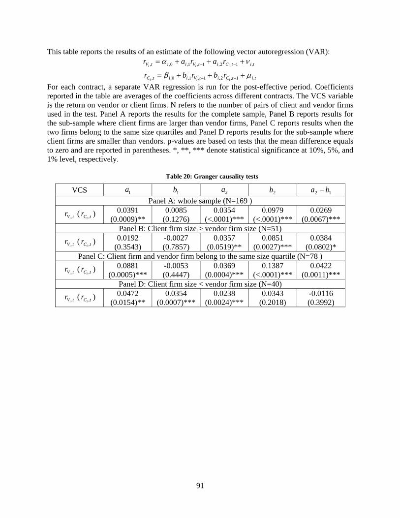
91

This table reports the results of an estimate of the following vector autoregression (VAR): titCitViitV iii

rarar ,1,2,1,1,0,, να +++= −−

titCitViitC iiirbrbr ,1,2,1,1,0,, μβ +++= −−

For each contract, a separate VAR regression is run for the post-effective period. Coefficients reported in the table are averages of the coefficients across different contracts. The VCS variable is the return on vendor or client firms. N refers to the number of pairs of client and vendor firms used in the test. Panel A reports the results for the complete sample, Panel B reports results for the sub-sample where client firms are larger than vendor firms, Panel C reports results when the two firms belong to the same size quartiles and Panel D reports results for the sub-sample where client firms are smaller than vendors. p-values are based on tests that the mean difference equals to zero and are reported in parentheses. *, **, *** denote statistical significance at 10%, 5%, and 1% level, respectively.

Table 20: Granger causality tests

VCS 1a 1b 2a 2b 12 ba − Panel A: whole sample (N=169 )

tVir , ( tCi

r , ) 0.0391 (0.0009)**

0.0085 (0.1276)

0.0354 (<.0001)***

0.0979 (<.0001)***

0.0269 (0.0067)***

Panel B: Client firm size > vendor firm size (N=51)

tVir , ( tCi

r , ) 0.0192 (0.3543)

-0.0027 (0.7857)

0.0357 (0.0519)**

0.0851 (0.0027)***

0.0384 (0.0802)*

Panel C: Client firm and vendor firm belong to the same size quartile (N=78 )

tVir , ( tCi

r , ) 0.0881 (0.0005)***

-0.0053 (0.4447)

0.0369 (0.0004)***

0.1387 (<.0001)***

0.0422 (0.0011)***

Panel D: Client firm size < vendor firm size (N=40)

tVir , ( tCi

r , ) 0.0472 (0.0154)**

0.0354 (0.0007)***

0.0238 (0.0024)***

0.0343 (0.2018)

-0.0116 (0.3992)

92

This table reports Pearson correlation coefficients for measures of accounting performance in the pre-effective and post-effective periods where year 0 is the year the contract goes into effect. p-values are reported in parentheses. *, **, *** denote statistical significance at 10%, 5%, and 1% level, respectively.

Table 21: Unadjusted accounting performance change cross-autocorrelation test

Correlation/ Year (-3, 0) (-2, 0) (-1, 0) (0, 1) (0,2) (0,3)

GRSMRGN 0.0157 (0.8772)

-0.0123 (0.8977)

-0.0132 (0.8866)

-0.0838 (0.3999)

-0.0464 (0.6750)

-0.0832 (0.5168)

NETMRGN 0.0863 (0.3932)

-0.0072 (0.9404)

-0.0276 (0.7657)

0.0371 (0.7098)

0.1792 (0.1001)*

0.0210 (0.8701)

TURNOVER 0.0314 (0.5215)

0.0299 (0.5341)

0.0130 (0.7858)

0.1345 (0.0133)***

0.1237 (0.0709)*

0.2661 (0.0018)***

ROA 0.0433 (0.1322)

0.0692 (0.1529)

0.0696 (0.1471)

0.8269 (<.0001)***

0.9840 (<.0001)***

0.2973 (0.0006)***

93

This table reports Pearson correlation coefficients for measures of accounting performance in the pre-effective and post-effective periods where year 0 is the year the contract goes into effect. The performance measures are adjusted the industry medians. p-values are reported in parentheses. *, **, *** denote statistical significance at 10%, 5%, and 1% level, respectively.

Table 22: Industry-median adjusted accounting performance change cross-autocorrelation tests

Correlation/ Year (-3, 0) (-2, 0) (-1, 0) (0, 1) (0, 2) (0, 3)

GRSMRGN 0.0542 (0.5925)

-0.0406 (0.6726)

-0.0133 (0.8857)

-0.0439 (0.6600)

-0.0122 (0.9121)

-0.0676 (0.5987)

NETMRGN 0.1030 (0.3076)

-0.0143 (0.8816)

-0.0235 (0.7999)

0.0434 (0.6635)

0.0008 (0.9944)

-0.0461 (0.7201)

TURNOVER 0.0658 (0.1785)

0.0381 (0.4273)

0.0393 (0.4095)

0.2107 (<.0001)***

0.2165 (0.0014)***

0.3365 (<.0001)***

ROA 0.0303 (0.5277)

0.0581 (0.2306)

0.0669 (0.1635)

0.8176 (<.0001)***

0.9640 (<.0001)***

0.1909 (0.0296)**

94

This table reports Pearson correlation coefficients for percentage changes in return on assets in the pre-effective and post-effective periods where year 0 is the year the contract goes into effect. p-values are reported in parentheses. *, **, *** denote statistical significance at 10%, 5%, and 1% level, respectively.

Table 23: Cross-autocorrelations of percentage changes in return on assets

(-3, 0) (-2, 0) (-1, 0) (0, 1) (0,2) (0,3) Panel A: Unadjusted change ratio cross-autocorrelation test

ROA -0.0530 (0.2844)

-0.0252 (0.6037)

0.0512 (0.2866)

0.9495 (<.0001)***

0.9990 (<.0001)***

0.1837 (0.0371)**

Panel B: Industry-median adjusted change ratio cross-autocorrelation test

ROA -0.0043 (0.9314)

0.0414 (0.3934)

0.0114 (0.8145)

0.3078 (<.0001)***

0.2585 (0.0002)***

0.0528 (0.5523)

Documents

The Short and Long-Run Financial Impact of Corporate