The shock waves in decaying supersonic turbulence · PDF fileties of the shock waves produced. ... The example we explore in detail is the decay of hyper-sonic hydrodynamic ... The

arX

iv:a

stro

-ph/

0002

291v

1 1

4 Fe

b 20

00

A&A manuscript no.(will be inserted by hand later)

Your thesaurus codes are:08 (02.08.1; 02.19.1; 02.20.1; 09.03.1; 09.11.1 )

ASTRONOMYAND

ASTROPHYSICS1.3.2018

The shock waves in decaying supersonic turbulence

Michael D. Smith1, Mordecai-Mark Mac Low2,3 & Julia M. Zuev4

1 Armagh Observatory, College Hill, Armagh BT61 9DG, Northern Ireland2 Max-Planck-Institut fur Astronomie, Konigstuhl 17, D-69117 Heidelberg, Germany3 Department of Astrophysics, American Museum of Natural History, 79th St. at Central Park West, New York, New York,10024-5192, USA4 JILA, University of Colorado, Boulder, Campus Box 440, Boulder, CO 80309, USAInternet: [email protected], [email protected], [email protected]

Received; accepted

Abstract. We here analyse numerical simulations of su-personic, hypersonic and magnetohydrodynamic turbu-lence that is free to decay. Our goals are to understandthe dynamics of the decay and the characteristic proper-ties of the shock waves produced. This will be useful forinterpretation of observations of both motions in molecu-lar clouds and sources of non-thermal radiation.

We find that decaying hypersonic turbulence possessesan exponential tail of fast shocks and an exponential de-cay in time, i.e. the number of shocks is proportional tot exp(−ktv) for shock velocity jump v and mean initialwavenumber k. In contrast to the velocity gradients, thevelocity Probability Distribution Function remains Gaus-sian with a more complex decay law.

The energy is dissipated not by fast shocks but by alarge number of low Mach number shocks. The power losspeaks near a low-speed turn-over in an exponential dis-tribution. An analytical extension of the mapping closuretechnique is able to predict the basic decay features. Ouranalytic description of the distribution of shock strengthsshould prove useful for direct modeling of observable emis-sion. We note that an exponential distribution of shockssuch as we find will, in general, generate very low excita-tion shock signatures.

Key words: Hydrodynamics – Turbulence –Shock waves– ISM: clouds – ISM: kinematics and dynamics

1. Introduction

Many structures we observe in the Universe have beenshaped by fluid turbulence. In astronomy, we often ob-serve high speed turbulence driven by supersonic ordered

Send offprint requests to: M.D. Smith

motions such as jets, supernova shocks and stellar winds(e.g. Franco & Carraminana 1999). Hypersonic speeds,with Mach numbers above 10, are commonly encountered.Clearly, to understand the structure, we require a theoryfor supersonic turbulence. Here, we concentrate on decay-ing turbulence, such as could be expected in the wakesof bow shocks, in the lobes of radio galaxies or followingexplosive events. Two motivating questions are: how fastdoes supersonic turbulence decay when not continuouslyreplenished and how can we distinguish decaying turbu-lence from other dynamical forms? The first question hasbeen answered through recent numerical simulations de-scribed below. The answer to the second question is soughthere. We look for a deep understanding of the dynamicsand physics which control decaying supersonic turbulence.From this, and a following study of driven turbulence, wecan derive the analytical characteristics and the observa-tional signatures pertaining to supersonic turbulence. Wecaution that we specify to uniform three dimensional tur-bulence with an isothermal equation of state, an initiallyuniform magnetic field and periodic boundary conditions.

Numerical studies of decaying supersonic turbulencein three dimensions have revealed a power-law decay ofthe energy in time following a short low-loss period (MacLow et al. 1998; Stone et al. 1998). Simulations of decay-ing subsonic and incompressible turbulence show similartemporal behaviour (e.g. Galtier et al. 1997), as discussedby Mac Low et al. (1999). In the numerical experiments,random Gaussian velocity fields were generated with smallwavenumber disturbances. Magnetic fields were includedof various strengths. Mac Low (1999) concluded that thedecay is so rapid under all conditions that the motions weobserve in molecular clouds must be continuously driven.In this work, we analyse the Mach 5 simulations from MacLow et al. (1998) as well as a new Mach 50 simulation.The hypersonic run should best illustrate the mechanisms

http://arxiv.org/abs/astro-ph/0002291v1

2 Smith, Mac Low & Zuev: Supersonic Turbulence

behind the development and evolution of the shock field,possibly revealing asymptotic solutions.

The major goal is to derive the spectrum of shocks(the Shock Probability Distribution Function) generatedby turbulence. Shocks are often responsible for detailedbright features, such as filamentary and sheet structures,within which particles are highly excited. An example ofa region which appears to contain a chaotic mixture ofshocks, termed a ’Supersonic Turbulent Reactor’ is theDR 21 molecular hydrogen outflow, driven by a collimatedwind from a high mass young star (Smith et al. 1998).The shock spectrum is related to the molecular excita-tion, with weak shocks being responsible for rotationalexcitation and strong shocks for vibrational excitation.

Previous studies of compressible turbulence have con-centrated on the density and velocity structure of the coldgas rather than the shocks. Three dimensional subsonicand transonic simulations (e.g. Porter et al. 1994; Fal-garone et al. 1994), two dimensional supersonic motions(Vazquez-Semadeni 1994) as well as three dimensionalsupersonic turbulence have been discussed (Vazquez-Semadeni et al. 1996, Padoan et al. 1998). One attemptsto describe and fit the density and velocity structures ob-served in molecular clouds. This is often appropriate forthe interpretation of clouds since, although the Mach num-ber is still high, the shock speeds are too low to producebright features. The simulations analysed here are also be-ing interpreted by Mac Low & Ossenkopf (2000) in termsof density structure.

Despite a diversity of theory, and an increase in ana-lytical knowledge, a succinct understanding of turbulencehas not been attained (see Lesieur 1997). Therefore, weneed not apologise for not fully interpreting the resultsfor the supersonic case. We do not look for a Kolmogorov-inspired theory for two reasons. First, fully developed tur-bulence becomes increasingly non-Gaussian towards smallscales. These intermittency effects dominate the statisticsof velocity jumps in supersonic turbulence. Second: thestrong compressibility implies that a wavenumber analy-sis is irrelevant since the energy spectrum of a shock or ofa system of shocks is simply k−2 (e.g. Gotoh & Kraich-nan 1993). Note that the Kolmogorov-like spectra foundby Porter et al. (1994) appeared at late times when theflow is clearly subsonic (and also note that even the initialRMS Mach number was only unity, which rather stretchesthe definition of supersonic turbulence).

We attempt here to construct a physical model todescribe the non-Gaussian Probability Density Functions(PDFs) for the shock waves. We adapt the mapping clo-sure analysis, as applied to Navier-Stokes (incompressible)and Burgers (one dimensional and pressure free) turbu-lence (Kraichnan 1990), to compressible turbulence. Phe-nomenological approaches, such as multifractal models orthe log-normal model, are avoided since they have lim-ited connection to the underlying physical mechanisms.In contrast, mapping closure follows the stretching and

squeezing of the fluid, and the competition between rampressure, viscosity and advection determines the spectralform.

We study here compressible turbulence without grav-ity, self-gravity or thermal conduction. No physical viscos-ity is modelled, but numerical viscosity remains present,and an artificial viscosity determines the dissipation in re-gions of strong convergence. By strong convergence, wemean high negative divergence of the velocity field, whichthus correspond to the shock zones as shown in Fig. 1.Periodic boundary conditions were chosen for the finitedifference ZEUS code simulations, fully described by MacLow et al. (1998).

The ZEUS code itself is a time-explicit second-orderaccurate finite difference code (Stone & Norman 1992a,b).It is ideal for problems involving supersonic flow and isversatile, robust and well-tested. Although higher ordercodes are potentially more accurate, the high speed of thealgorithms means that large problems can be solved athigh resolution. This enables us to test for convergenceof the energy dissipation rate (Mac Low et al. 1998),shock distributions (Sect. 2.4) and numerical viscosity(Sect. 2.6). Furthermore, the basic hydrocode results havebeen confirmed on solving the same problems with thecontrasting method of smoothed particle hydrodynamics(Mac Low et al. 1998). The constrained transport algo-rithm (Evans & Hawley 1988) updated through use of themethod of characteristics (Hawley & Stone 1995) is usedto maintain a divergence-free magnetic field to machineaccuracy and to properly upwind the advection.

We begin by discussing the method used to countshocks from grid-based simulations (Sect. 2.1-2.2). Wethen present the shock jump PDFs and provide analyticalfits for the hypersonic M = 50 case (Sect. 2.3-2.5). Theone-dimensional counting procedures are verified througha comparison with full three-dimensional integrations ofthe dissipated energy (Sect. 2.6). Supersonic hydrody-namic M = 5 (Sect. 3) and magnetohydrodynamic (Alfvennumbers A = 1 and A = 5) simulations (Sect. 4) are thenthen likewise explored. Note the definition of the AlfvenMach number A = vrms/vA, where v2A = B2/4πρ wherevrms is the initial root mean square (RMS) velocity and vAis the Alfven speed. The evolution of the velocity PDFsare then presented and modelled (Sect. 5). Finally, we in-terpret the results in terms of the dynamical models (Sect.6).

2. Hydrodynamic hypersonic turbulence

2.1. Model description

The example we explore in detail is the decay of hyper-sonic hydrodynamic turbulence (Fig. 1). The three dimen-sional numerical simulation on a D3 = 2563 grid with peri-odic boundary conditions began with a root mean squareMach number of M = 50. The initial density is uniform

Smith, Mac Low & Zuev: Supersonic Turbulence 3

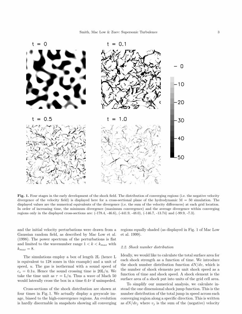
Fig. 1. Four stages in the early development of the shock field. The distribution of converging regions (i.e. the negative velocitydivergence of the velocity field) is displayed here for a cross-sectional plane of the hydrodynamic M = 50 simulation. Thedisplayed values are the numerical equivalents of the divergence (i.e. the sum of the velocity differences) at each grid location.In order of increasing time, the minimum divergence (maximum convergence) and the average divergence within convergingregions only in the displayed cross-sections are: (-178.4, -46.6), (-441.9, -48.0), (-146.7, -13.74) and (-99.9, -7.3).

and the initial velocity perturbations were drawn from aGaussian random field, as described by Mac Low et al.(1998). The power spectrum of the perturbations is flatand limited to the wavenumber range 1 < k < kmax withkmax = 8.

The simulations employ a box of length 2L (hence Lis equivalent to 128 zones in this example) and a unit ofspeed, u. The gas is isothermal with a sound speed ofcs = 0.1u. Hence the sound crossing time is 20L/u. Wetake the time unit as τ = L/u. Thus a wave of Mach 50would laterally cross the box in a time 0.4τ if unimpeded.

Cross-sections of the shock distribution are shown atfour times in Fig. 1. We actually display a greyscale im-age, biased to the high-convergence regions. An evolutionis hardly discernable in snapshots showing all converging

regions equally shaded (as displayed in Fig. 1 of Mac Lowet al. 1999).

2.2. Shock number distribution

Ideally, we would like to calculate the total surface area foreach shock strength as a function of time. We introducethe shock number distribution function dN/dv, which isthe number of shock elements per unit shock speed as afunction of time and shock speed. A shock element is thesurface area of a shock put into units of the grid cell area.

To simplify our numerical analysis, we calculate in-stead the one dimensional shock jump function. This is thenumber distribution of the total jump in speed across eachconverging region along a specific direction. This is writtenas dN/dvj where vj is the sum of the (negative) velocity


gradients (i.e. Σ [−δvx] across a region being compressedin the x-direction). We employ the jump Mach number inthe x-direction Mj = vj/cs rather than vj since this is theparameter relevant to the dynamics. Thus, each boundedregion of convergence in the x-direction counts as a singleshock and the total jump in Mj across this region is takenas its strength.

Numerically, over the whole simulation grid (x,y,z), wecalculate each shock jump through

Mj =

x=xf∑

x=xi

(∆vx/cs) (1)

with the condition that ∆vx < 0 in the range xi ≤ x < xf .This is then binned as a single shock element. The shocknumber distribution dN/dMj is obviously dimensionless.

The 1D approach neglects both the shock angle andfull shock strength. The distribution of shock jumps, how-ever, is found by adding up an enormous number of con-tributions over the whole grid. This method has the ad-vantage of being extremely robust, involving no model as-sumptions. To be a direct representation of the true shockstrength function, however, it requires a few assumptionsto be justified: (1) a one-dimensional shock jump is re-lated to the actual shock speed, (2) not too many shocksare excluded because their surfaces are aligned with thechosen direction, (3) the shock velocities are distributedisotropically and (4) unsteepened compressional waves canbe distinguished from true shocks.

First, we note that it is an extremely difficult taskto calculate the actual shock speed for each shock. Itis, however, unnecessary since the shock speed and one-dimensional shock jump are closely related statistically.We also take the number of zones at which compressivejumps are initiated as the number of shocks (where shocksare colliding, the method will be inaccurate). Assumption(3) will not hold for the magnetohydrodynamic turbulencewhich has a defined direction. In these cases, the jump dis-tributions must be calculated both parallel and transverseto the original magnetic field. Assumption (4) will not bemade: we include all acoustic waves, but we have followedthe width of the jumps and so can verify whether shocksor waves are being counted. This is important since broadcompressional waves also dissipate energy and become in-creasingly significant, of course, as the high-speed shocksdecay and the flow eventually becomes subsonic.

Many shock surfaces are distorted, occasionally bow-shaped. This does not negate our counting procedure pro-vided the curvature is not too strong. Here the relevantlengths are the shock radius of curvature and the shockwidth. The latter is determined by our numerical method,involving von Neumann & Richtmyer (1950) artificial vis-cosity, which here constrains strong shocks to just a fewzones. As seen from Fig. 1, we can confidently take one-dimensional cuts across the shock surfaces and equate the

measured jump to the actual jump in speed of fluid ele-ments to a good first approximation.

In Sect. 2.6, we check our method by demanding con-sistency with integrated quantities derived directly fromthe numerical simulations.

2.3. Hypersonic turbulence

The randomGaussian field rapidly transforms into a shockfield in the Mach 50 case (Fig. 1). The shock steepeningis reflected in the initial increase in the minimum value ofthe divergence (see the caption to Fig. 1). Note that theaverage value of the divergence does not change i.e. thetotal number of converging zones only falls from half toabout one third, despite the steepening. The explanationis that the shocks have time to form in the strongly con-verging regions but the compression in most of the flowprogresses slowly. After the time t = 0.1, the number offast shocks decays and the average convergence decreases.The total number of zones with convergence, however, re-mains constant throughout. This fact, that the total shocksurface area is roughly conserved, is verified in the follow-ing analysis.

The one-dimensional distribution of the number ofshock jumps as a function of time is presented in Fig. 2 forthe case with RMS Mach number M = 50. This demon-strates that the shock jump function both decays andsteepens. One can contrast this to the decay of incom-pressible turbulence where the distribution function, asmeasured by wavenumber, maintains the canonical Kol-mogorov power-law in the inertial range during the decay(Lesieur 1997). Here we remark that a power-law fit is im-possible (Fig. 2a) but stress that this result applies onlyto the case at hand: decaying turbulence.

The jump distribution is very close to being exponen-tial in both velocity and time. This remarkably simpleconclusion is based on the good fits shown in Fig. 2b. Notethat the pure exponential only applies to the medium andstrong shock regime. To also account for the low Machnumber regime, we fitted a further time dependence asshown in Fig. 3, yielding

dN

dMj= 105.72 t exp(−Mj t/2.0) (2)

in terms of the 1-D jump Mach number. Better fits canbe obtained with a somewhat more complex time depen-dence. We find excellent fits for

dN

dMj= 105.79 t exp [− βMj t

α] (3)

with α ∼ 0.88 ± 0.03 and β ∼ 0.52 ± 0.03. The valuesand errors are derived from parameter fitting of all thedisplayed curves to within a factor of ∼ 1.5. We exclude inthis process the phase where collisional equilibrium wouldnot be expected: at early times and low Mach numberstMj < 0.5. Also, we exclude the jump speeds where thejump counts are low (shock numbers dN/dMj < 3000).


Fig. 2. The jump velocity distribution. Two representations of the number of compressive layers in the x-direction as a functionof the total x-speed change across the layer at 10 equally-spaced times beginning at time t = 0.5 (solid line) and continuing,with a monotonic decay of the high-speed jumps, in time steps of 0.5. They demonstrate the decay and steepening and that (a)no power law can represent the behaviour at any stage, and (b) a series of exponentials of the form exp(−t(vj − 2)/2) fit thehigh velocities well.

Fig. 3. The jump velocity distribution extracted from the M = 50 hydrodynamic simulation as a function of time, as in Fig. 2.The fitted function is dN/dMj = 105.42 t exp(−tMj/2).


Fig. 4. The evolution of the jump velocity distribution at tworesolutions for M = 50 hydrodynamic simulation with kmax =2. The shock number for the 643 simulation has been multipliedby 4 to adjust for the larger zone sizes.

2.4. Convergence and dependence on initial conditions

Resolution studies are essential to confirm numerical re-sults. One hopes that the results demonstrate conver-gence. This is plausible for supersonic flow in which thedecay does not depend on the details of the viscosity orthe details of the shock transitions. This has been con-firmed for the analysis of the total energy (Mac Low et al.1998).

We compare available simulations for the hypersonicstudy with 643 and 1283. We also set the initial wavenum-ber range to kmax = 2 and can thus examine the depen-dence on the chosen initial state.

The results at the two different resolutions are inquite good agreement, especially in the high Mach numberregime (Fig. 4). The density of high Mach number shocksis quite low and they are well resolved. At low Mach num-bers, the lower resolution simulation fails, of course, tocapture the vast quantities of weak compressional wavescontained in the higher resolution example. It is to be ex-pected that shock turbulence configurations get extremelycomplex on small scales, through the interactions whichproduce triple-point and slip-layer structures. To capturethis structure requires adaptive grid codes. This does notmean, however, that the simulations are inaccurate for ourpurposes since energy dissipation is not controlled by theweak shocks until very late times, as verified in Fig. 5.

A similar formula for the shock jump function is found.The evolution, however, is three times slower. We show inFig. 6 the model fit

dN

dMj= 104.23 t exp(−Mj t/6.0). (4)

Fig. 6. The jump velocity distribution extracted fromthe 1283 M = 50 hydrodynamic simulation with kmax

= 2 as a function of time. The fitted function isdN/dMj = 103.93 t exp(−tMj/6).

This suggests that the rate of decay is proportional tothe initial mean wavenumber of the wave distribution. Thedecay kmax = 2 simulation is a factor of three slower thanin the kmax = 8 simulation. The mean wavenumber ofthe two simulations are km = 1.5 and 4.5, with flat initialenergy distributions. Hence, given that Mj = vx/cs and tis in units of L/10cs, the shock numbers are approximately∝ t exp(−kot vj) where ko ∼ 1.1 km. The dependence onthe initial mean wavenumber is expected since the boxsize should not influence the decay rate if we are indeed,as we wish, following the unbounded decay.

Note that two parameter fitting, as above, in this caseyields

dN

dMj= 104.23 t exp [− βMj t

α] (5)

with α ∼ 1.02± 0.03 and β ∼ 0.168± 0.008.

2.5. Shock power distribution

How is the spectrum of shock jumps related to the decayof energy? Here we show that the energy dissipation inthe fast shocks is directly correlated with their numberwhich is decreasing exponentially. Furthermore, the weak-est shocks, which merge into an area of ’compressionalwaves’, are ineffective in the overall dissipation. The resultis that the moderately-supersonic part of the turbulencerapidly becomes and remains responsible for the energydissipation for an extended time.

The shock power distribution function is here definedas the energy dissipated per unit time per unit jump speedvj as a function of jump speed. Here again we employ theuni-directional jump Mach number Mj . We actually cal-culate the energy dissipated by artificial viscosity acting


Fig. 5. The power dissipated as a function of the jump velocity. The power is displayed per unit Mj where Mj = vj/cs,and the data is extracted from the M = 50 hydrodynamic simulation for times t = 1,2,3,4 & 5. The fitted function isdE/dMj = 0.016 tM2.5

j exp(−tMj/2).

along a specific direction within the shocks as defined byconvergence along this direction. Hence we anticipate thatin isotropic turbulence one third of the full loss will be ob-tained. The relative contributions of artificial and numer-ical viscosity, which also confirms the method employedhere, are discussed in Sect. 2.5.

The jump number distribution includes a high propor-tion of very weak compressional waves that dissipate lit-tle energy. The one-dimensional shock power distribution,dE/dMj , shown in Fig. 5, illustrates this. The functionalfit is guided by the above shock number distributions,which we would expect to remain accurate for the highMach number jumps. We display the fit to:

dE

dMj= 0.016M2.5

j t exp(−kMj t) (6)

with k = 0.5, which is again remarkably accurate giventhe lack of adjustable parameters. Hence dE/dMj ∝M2.5

j dN/dMj. Note that the energy dissipated across anisothermal steady shock of Mach number M and pre-shockdensity ρ is Es = (ρc3s/2)M

3(1 - 1/M2) and that the jump

in Mach number is MJ = M(1 - 1/M2). This yields

Es = 0.5 ρc3s M3J

[

1 +

√(1 + 4/M2

J) − 1

2

]

. (7)

Therefore, the numerical result suggests a (statistical) in-verse correlation between density and shock strength.

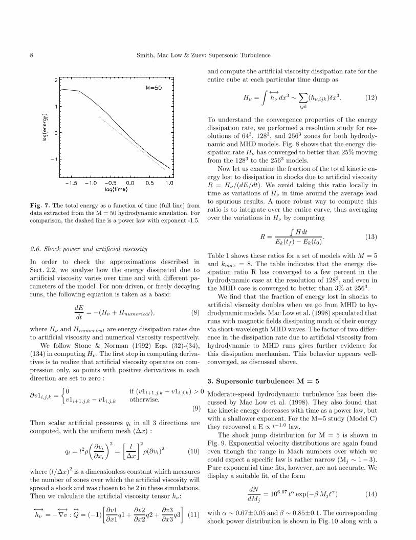
Note that Eq. 6 yields E ∝ t−2.5 (on integrating overMj and substituting the variable w = Mjt) Thus, oneobtains a power-law decay in total energy of the form E∝ t−1.5. This behaviour of the total energy decay and theenergy dissipation rate, is indeed found in the simulations,as shown in Fig. 7. Hence the results are fully consistentwith the simple fits. Note that the energy decay deviatesfrom a pure power law: there is an early transition phasebetween times t = 0.1 - 0.5 during which the decay ismore rapid (Fig. 7). This was not found in simulations ofmoderate Mach number supersonic turbulence (Mac Lowet al. 1998) but appears here and also in simulations inwhich the supersonic turbulence is initially driven (MacLow 1999).


Fig. 7. The total energy as a function of time (full line) fromdata extracted from the M = 50 hydrodynamic simulation. Forcomparison, the dashed line is a power law with exponent -1.5.

2.6. Shock power and artificial viscosity

In order to check the approximations described inSect. 2.2, we analyse how the energy dissipated due toartificial viscosity varies over time and with different pa-rameters of the model. For non-driven, or freely decayingruns, the following equation is taken as a basic:

dE

dt= −(Hν +Hnumerical), (8)

where Hν and Hnumerical are energy dissipation rates dueto artificial viscosity and numerical viscosity respectively.

We follow Stone & Norman (1992) Eqs. (32)-(34),(134) in computingHν . The first step in computing deriva-tives is to realize that artificial viscosity operates on com-pression only, so points with positive derivatives in eachdirection are set to zero :

∂v1i,j,k =

{

0 if (v1i+1,j,k − v1i,j,k) > 0v1i+1,j,k − v1i,j,k otherwise.

(9)

Then scalar artificial pressures qi in all 3 directions arecomputed, with the uniform mesh (∆x) :

qi = l2ρ

(

∂vi∂xi

)2

=

[

l

∆x

]2

ρ(∂vi)2

(10)

where (l/∆x)2 is a dimensionless constant which measuresthe number of zones over which the artificial viscosity willspread a shock and was chosen to be 2 in these simulations.Then we calculate the artificial viscosity tensor hν :

←→

hν = −←→

∇v :↔

Q = (−1)

[

∂v1

∂x1q1 +

∂v2

∂x2q2 +

∂v3

∂x3q3

]

(11)

and compute the artificial viscosity dissipation rate for theentire cube at each particular time dump as

Hν =

∫

←→

hν dx3 ∼

∑

ijk

(hν,ijk)δx3. (12)

To understand the convergence properties of the energydissipation rate, we performed a resolution study for res-olutions of 643, 1283, and 2563 zones for both hydrody-namic and MHD models. Fig. 8 shows that the energy dis-sipation rateHν has converged to better than 25% movingfrom the 1283 to the 2563 models.

Now let us examine the fraction of the total kinetic en-ergy lost to dissipation in shocks due to artificial viscosityR = Hν/(dE/dt). We avoid taking this ratio locally intime as variations of Hν in time around the average leadto spurious results. A more robust way to compute thisratio is to integrate over the entire curve, thus averagingover the variations in Hν by computing

R =

∫

Hdt

Ek(tf )− Ek(t0). (13)

Table 1 shows these ratios for a set of models with M = 5and kmax = 8. The table indicates that the energy dis-sipation ratio R has converged to a few percent in thehydrodynamic case at the resolution of 1283, and even inthe MHD case is converged to better than 3% at 2563.

We find that the fraction of energy lost in shocks toartificial viscosity doubles when we go from MHD to hy-drodynamic models. Mac Low et al. (1998) speculated thatruns with magnetic fields dissipating much of their energyvia short-wavelengthMHD waves. The factor of two differ-ence in the dissipation rate due to artificial viscosity fromhydrodynamic to MHD runs gives further evidence forthis dissipation mechanism. This behavior appears well-converged, as discussed above.

3. Supersonic turbulence: M = 5

Moderate-speed hydrodynamic turbulence has been dis-cussed by Mac Low et al. (1998). They also found thatthe kinetic energy decreases with time as a power law, butwith a shallower exponent. For the M=5 study (Model C)they recovered a E ∝ t−1.0 law.

The shock jump distribution for M = 5 is shown inFig. 9. Exponential velocity distributions are again foundeven though the range in Mach numbers over which wecould expect a specific law is rather narrow (Mj ∼ 1− 3).Pure exponential time fits, however, are not accurate. Wedisplay a suitable fit, of the form

dN

dMj= 106.07 tα exp(−βMjt

α) (14)

with α ∼ 0.67±0.05 and β ∼ 0.85±0.1. The correspondingshock power distribution is shown in Fig. 10 along with a


Comparison of Ratios

run B C D N P Q J L

grid 643 1283 2563 643 1283 2563 643 2563

physics Hydro Hydro Hydro MHD MHD MHD MHD MHDA ∞ ∞ ∞ 1 1 1 5 5R 0.62 0.68 0.68 0.38 0.36 0.35 0.59 0.49

Table 1. The fraction of the energy dissipated through artificial viscosity for models of supersonic turbulence. Ratio R is definedby Eq. (13). Model labels correspond to those of Table 1 of Mac Low et al. (1998). A is the RMS Alfven Mach number.

Fig. 9. The jump velocity distribution extracted from the M = 5 hydrodynamic simulation (Mac Low et al. 1998) as a functionof time. The fitted function is exponential in velocity but more complicated in time (see text) (α = 0.67 and β = 0.85 displayed).The time sequence shown is t = 1,2,3,5 and 10.

best-fit family of curves calculated from

dE

dMj= 0.10M3.6

j tα exp(−βMjtα) (15)

with α = 0.62 ± 0.04 and β = 1.6 ± 0.1.Hence, an ex-ponential velocity distribution is maintained. The decay,however, is slightly slower. Integrating over Mj , yieldsE ∝ t−1.00.

Integrating overMj, with the limits of integration from0 to ∞ (to account for all the jumps), and with the sub-stitution x = Mtα, we observe that the integral becomestime-independent. Thus, integration of Eq. 15 over Mj

yields dE/dt ∝ t−2.23. This yields dE/dt ∝ t−1.23, whichis quite close to the E ∝ t−1 law found by Mac Low et al.(1998).

Now we want to compare how the two quantities varywith time: dE/dt from Eq. 15 and the energy dissipationrate due to artificial viscosity Hν , derived using the algo-rithm discussed in Sect. 2.6. Fig. 11 shows that the twomethods indeed agree. Thus, the shock power distributionmethod (Sect. 2.6) confirms that the statistical approachworks with power calculations for each 1D converging re-gion.


Fig. 10. The power dissipated as a function of the jump velocity. The power is displayed per unit Mj where Mj = vj/cs, andthe data is extracted from the M = 5 hydrodynamic simulation for times t = 1,2,3,4 & 5. The fitted function, given in the text,takes α = 0.62 and β = 1.6.

4. MHD turbulence: M = 5, A = 1 and 5

An analysis of simulations of MHD turbulence allows usto determine which wave modes are involved. The timedependence of the kinetic energy of freely decaying MHDturbulence has been discussed by Mac Low et al. (1998).Remarkably, the kinetic energy also decreases with timeas a power law, although with only a slightly shallower ex-ponent than the equivalent hydrodynamic simulation. Weconsider here the high-field example in which the initialRMS Mach number M = 5 and the initial RMS Alfvennumber A is unity and the low-field equivalent with A =5. Mac Low et al. recovered: E ∝ t−0.87. (at the highestresolution of 2563) for the high field case.

The initial field configuration is simply a uniform fieldaligned with the z-axis. Thus the imposed velocity fieldcontrols the turbulent energy input, and some energy issubsequently transferred into magnetic waves. We imposeno turbulent diffusion here: magnetic energy may, how-ever, still be lost through numerical diffusion or MHDwave processes.

The jump number distribution function for these sim-ulation (Fig. 12) possesses exponential velocity distribu-

tions over a range in Mj . The displayed fit to the highfield case (Fig. 13) is

dN

dMj= 105.94 tα exp(−βMjt

α). (16)

where α ∼ 0.66 ± 0.03 and β ∼ 0.62 ± 0.03. For the A =5 case, α ∼ 0.57± 0.03 and β ∼ 1.01± 0.05.

This analysis indicates that (1) supersonic MHD tur-bulence is, mathematically at least, no different from hy-drodynamic turbulence in that the shock distribution isexponential and (2) the time dependencies are also sim-ilar to the hydrodynamic M = 5 case. From Fig. 12, weconclude (1) that the distribution of high speed shocks re-mains unchanged and isotropic in the low-field case, (2)the distribution of transverse waves is somewhat faster todecay when a weak field is present, whereas in the strongfield case (3) the high speed transverse waves survive sig-nificantly longer from the outset and (4) the whole spec-trum of parallel waves is suppressed by a factor ∼ 2.

The velocity jump distributions plotted here are a com-bination of shocks and waves. Due to the high Alfvenspeed, the shocks are predominantly slow shocks in the


Fig. 8. Resolution study for 3D models – Energy dissipationrate due to artificial viscosity versus time. Top graph: modelB (643, triangle), model C (1283, dashed line), and modelD (2563, solid line). Bottom graph: model N (643, triangle),model P (1283, dashed line), and model Q (2563, solid line).For hydrodynamic models we observe that the energy dissipa-tion rate Hν has converged to better than 35% moving from643 to the 1283 models, and to better than 25% moving fromthe 1283 to the 2563 models. These values are 37% and 23% forthe MHD models. Thus, energy dissipation rate due to artificialviscosity converges as we go to finer grids.

Fig. 11. Top: dE/dt versus time - the graph presents Hν formodel C (grid 128, M=5, hydrodynamic) for 21 time dumps(rhombs), and integral of Eq. (8) over dMj (solid line). Bothare energy dissipation rates due to artificial viscosity. We see aclose fit of the methods. For comparison, dashed line representstotal kinetic energy changes dE/dt directly from the numericalsimulation output. Bottom: the absolute value of the relativeerror between Hν and integrated Eq. (15).

A = 1 case. These shocks can propagate with wave vec-tors in all directions except precisely transverse to thefield. Their propagation speeds are relatively slow sincethe (initially-uniform) Alfven speed is 5 times the soundspeed), and therefore their energy may be transferred intofaster waves via the turbulence raised in the magneticfield. In any case, it appears from Fig. 12 that about two-thirds of the compressional wave/shock energy is in trans-verse compression modes for the case A = 1. The wavesin this case, as measured here by regions of convergencealong the axes, are fast magnetosonic waves (close to com-pressional Alfven waves). The proportion of each can beestimated from the simulations by calculating the jumpwidths (in practice, we here place the extra requirementthat the one-dimensional jump across each individual zoneexceeds 0.2 cs, in order to distinguish the shocks from the


Fig. 12. The jump velocity distribution extracted from the M= 5 low magnetic field (A = 5) and high field (A = 1) MHD2563 simulations (Mac Low et al. 1998) as a function of time.The 5 times shown are t = 1,2,3,6 and 10. The two curvesshown for each time are the velocity jumps transverse to thefield (dashed) and parallel to the field (solid lines). The fittedexponentials are described in the text.

waves). We then find that at Mj = 1, just over half thejumps are slow shocks (with an average resolution of ∼ 3.0and 3.3 zones transverse and parallel, respectively), whilefor Mj > 4, 76% of the ’jumps’ are actually waves (an aver-age of ∼ 6.0 and 7.7 zones in each converging region). Thiscontrasts with the hydrodynamic simulations where, quiteuniformly, well over 90 % of the jumps are indeed narrowshocks, resolved only by the artificial viscosity. These areof course estimates which ignore the possibility that manyflow regions may be quite complex combinations of wavesand shocks.

An explanation of why such different types of turbu-lence decay in the same functional manner is offered inSect. 6.5.

Fig. 13. Exponential fits to the jump velocity distributions forthe high magnetic field (M = 5, A = 1) MHD 2563 simulation.A mean value for the number of shocks in each direction hasbeen taken. The 5 times shown are t = 1,2,3,6 and 10. Thefitted exponentials are described in the text with α = 0.66 andβ = 0.62.

5. The probability distribution functions

A traditional aid to understanding numerically-createdturbulence is the probability distribution function (PDF)of the velocities. Here, we determine the one-dimensionalMass Distribution Function by calculating the mass perunit Mach number interval of the motion in the x-direction. Note all zones contribute here, whether in theshocks or not.

We recover Gaussian distributions in the velocity, asapparent in Fig. 14. This is clearly displayed on a Mass-log(M2) plot for the high-speed wings (Fig. 15) where aGaussian would generate a linear relationship. Note thateach time step produces two lines, one for positive andone for negative absolute velocities. At early times, theimposed symmetry is still dominant but later on, smallasymmetries become more apparent. To estimate the timedependence we have taken the mean mass fraction of eachpair, on defining the initial mass density to be unity (i.e.a unit mass is initially contained in a box of size L3) andfound that a fit of the form

d(mass)

dM= 1.6 t0.75 exp(−0.088M2t1.5) (17)

is reasonable (Fig. 16). Interestingly, the decay in time ofthe PDF is not exponential. It is a faster decay law thanfor the shocks. This is inherent to the nature of decayingturbulence: in the beginning, closely-following shocks ac-celerate the fluid to high speeds. At late times, the fastshocks are quite evenly spread out and do not combine toproduce high acceleration.


Fig. 14. The decay of the PDF for the M=50 simulation. Thedistributions are shown for the 8 equal time steps from 0.5 to4

Fig. 15. A log-v2 display of the decay of the PDF for the M=50simulation demonstrates the Gaussian nature of the PDFs.The distributions for positive and negative absolute speeds areshown for the 8 equal time steps from 0.5 to 4, in descendingorder.

6. Interpretation of shock number distribution

6.1. The mapping closure method

A satisfying understanding of turbulence has been elu-sive. One can hope that supersonic turbulence may pos-sess some simplifying aspects. We have thus devoted muchtime trying to interpret the above shock distributions ofdecaying turbulence. In this section, we first relate the nu-merical simulations to theoretical models which have pre-

Fig. 16. Fits (dashed lines) to the decay of the PDF for theM=50 simulation. The mean distributions (full lines) are shownfor the 8 equal time steps from 0.5 to 4. The model fits are givenby Eq. 17, which is tailored so that the total mass in the boxis conserved.

dicted exponential velocity gradient PDFs for other formsof turbulence. We then interpret the evolution of the shockPDFs with an extension of these models utilising the bal-listic (ram pressure) principles behind hypersonic turbu-lence.

We require a model based on local interaction in phys-ical space in order to model shock interactions. We adaptthe heuristic ‘mapping closure’ model in the form pre-sented by Kraichnan (1990), in which analytical approx-imations were used to describe the evolution of Burg-ers turbulence. First, the initial competition between thesqueezing and viscous processes is followed. An assumedGaussian reference field is distorted non-linearly in timeinto a dynamically evolving non-Gaussian field. Velocityamplitude and physical space are remapped by choosingtransformations of particular forms. The PDF of a two-point velocity difference changes smoothly from Gaussianat very large separations (relating independent points) tosome function ξ at small distances. The mapping functionsare then determined by matching the evolution equationswith the dynamical equations. The closure is obtained bylimiting the form of the distortions to locally determinedtransformations.

The model for Burgers turbulence provides our inspira-tion since, in the hypersonic flow simulations of isothermalgas, thermal pressure is only significant within the thinshock fronts. Furthermore, individual shock structures arepredominantly one-dimensional. Care must be exercised,however, since regions of vorticity are created behindcurved shocks which are absent in the one-dimensionalBurgers turbulence.


6.2. Background formulation

We assume a known reference field for the initial velocityuo(z) as a function of a reference coordinate system z(Gotoh & Kraichnan 1993). The ’surrogate’ velocity fieldis u(x, t) and is related to uo and the reference coordinatesby vector and tensor mapping functions X and J:

ui = Xi(uo, t), (18)

∂zi/∂xj = Jij(uo, ξo, t) (19)

where reference velocity gradients are ξij,o = ∂ui,o/∂zjand velocity gradients are ξij = ∂ui/∂xj. The goal is tofind the distortions described by X and J for which thesurrogate velocity field is a valid approximation to the ve-locity field as given by the equations of motion. The abovetransformations, however, constrain the allowed forms ofhigher order statistics and, hence, neglect some physicswhich affect the long-term evolution (Gotoh & Kraichnan1993).

Mapping closure also assumes that the velocity PDFsP (uo) and P (u) are related to multivariate-Gaussiansthrough prescribed forms. The justification is simply thestatistical mechanics argument, as applied to particlespeeds in equilibrium thermodynamics. The velocity gra-dient PDF is written as Q(ξ, t) with u and ξ taken to bestatistically independent.

For convenience, we concentrate on the component ofthe velocity, ui, in the xi direction. We rewrite the decayof velocity amplitudes in the simpler form

ui = Xi(uo, t) = ri(t)ui,o(zi), (20)

and the velocity gradients then map through

∂ui

∂xi= ξii = ri(t)ξii,oJii(uo, ξo, t) = Yii(ξo, t), (21)

so defining Y. The velocity gradient PDF, which containsthe shock PDF, can now be written

Q(ξii) = Qo(ξii,o)

[

ξiiξii,o

]

−1N

Jii(22)

where N(t) normalises the PDF. This is the framework inwhich we can discuss the statistical evolution of velocitygradients.

6.3. Dynamical input

The momentum equations being solved, with the pres-sure gradients neglected, areDui/Dt = (1/ρ)(∂/∂xj)µσi,j

where Dui/Dt = ∂ui/∂t + uj∂ui/∂xj , σi,j is the stresstensor and µ is the viscosity. Differentiation yields the ve-locity gradient equation:

DξiiDt

+ ξikξki = −1

ρ

∂

∂xi

∂

∂xj(µσi,j) (23)

where the usual summation rule applies to j and k (but iis a chosen direction).

To continue, we can derive the evolution of the func-tions J, by equatingQ(ξ, t) as derived from these equations(yielding a rather complex form of the reduced Liouvilleequation, see Gotoh & Kraichnan 1993) with the Q derivedfrom the mapping closure approximation (Eq. 22). Then,however, the analysis becomes mathematically dense andnumerical solutions are probably the best option.

We here revert to a simple heuristic form of mappingclosure, taking ξ to be any component of ξii and the map-ping function J = Jii to be determined by requiring theprobability function Q as derived from substituting forDξ/Dt from the reduced Eq. 23 into the reduced Liouvilleequation,

∂Q

∂t+

∂

∂ξ

(

[

Dξ

Dt

]

c:u,ξ

Q

)

= ξQ, (24)

(where [..]c:u,ξ denotes the ensemble mean conditional ongiven values of u and ξ) to be equal to the Q derived fromthe equivalent for mapping closure (see Gotoh & Kraich-nan 1993),

∂Q(ξ, t)

∂t+

∂

∂ξ

(

∂Y (ξo, t)

∂tQ(ξ, t)

)

= γQ(ξ, t), (25)

where γ = (∂/∂t) ln(N/J). After some manipulation, thisyields an equation for the evolution of J of the form (seealso Eq. 24 of Gotoh & Kraichnan (1993))

∂J

∂t= −rξoJ

2 − µk2dJ3 +D(J3) (26)

where k2d = 〈(∂ξo/∂z)2〉/〈ξ2o〉, angled brackets denotingthe ensemble mean and D(J3) is a function consisting offurther non-linear derivative terms of the form J3. Also,an integral term involving Q is neglected here, which a

posteriori limits the solutions to high jump Mach numbers|ξ| > r2χo (χo being defined below)

Note that the left hand side and the first two termson the right are close to the Navier-Stokes form given byKraichnan (1990), with the addition of the function r = riwhich accounts for compressibility. These terms providethe statistics of the field through a non-linear transfor-mation of the initial field with known statistics. The fi-nal term combines together non-linear derivatives, a stepwhich permits further manipulation but with the loss ofinformation concerning the constants of integration.

The evolution of J begins rapidly by the steepeningof large velocity gradients (first term on the right), untilbalance with the viscous term (second term on the righthand side) is achieved. Equating these two terms yieldsthe form of the mapping function: J = −rξo/(µk

2d). Sub-

stitution into Eq. 21 yields ξ = −r2(t)ξo2/(µk2d). We con-

vert the initial Gaussian PDF Qo(ξo) into Q1(ξ1) by using


Eq. 22 to yield the result that the velocity gradient PDFis transformed into an exponential function:

Q1(ξ1) =

( 〈ξ2o〉8πr2χ2

o

)1

2 N(t)

|ξ1|exp

[

− |ξ1|2r2χo

]

(27)

where χo = 〈ξ2o〉/(νk2d). This function has been derivedfor the high gradients i.e. the shocks, consistent with thenumerical simulations.

The exponential being set up, the gradients are thendetermined by the inviscid terms. Thus, the continued evo-lution of J is described by the first two terms in Eq. 26which, on substituting the mapping J = ξ/(rξ1) yield

∂

∂t

(

ξ/ξ1r

)

= ξ1(ξ/ξ1)

2

r. (28)

This has an asymptotic power law solution of the formξ/ξ1 = 1/(1+ t/(t1)), t1 being a constant. Hence, at larget, the velocity gradient associated with a fluid trajectory isinversely proportional to time, as physically plausible for ahigh Mach number expanding flow. Substituting ξ1 = (1+t/t1)ξ for ξ1 in Eq. 27, and normalising the PDF throughN, yields

Q(ξ) = kξoξexp

[

− ξt

χξoto

]

. (29)

for large t, where χ = 2 r2o〈ξ2o〉/(µk2dξo) and k is a constant.Hence, mapping closure predicts, for zero-pressure hydro-dynamic flow, the same fast shock decay law as uncoveredin the hypersonic simulations.

The above mapping closure technique provides insightinto the rapid build up of velocity gradients and transfor-mation to an exponential, as well as the evolution of theexponential term. The form of the prefactor excludes anextension to low speeds.

6.4. A direct physical model

The interpretation we now present is an extension of thedynamic basis of the mapping closure model. First, weneglect viscosity since the long term evolution must bederivable from purely inviscid theory. The critical addi-tion to the above analysis is a result of the simulations: thetotal number of zones across which the gas is convergingremains at approximately 30%, independent of time. Thiscan also be derived from integrating Eqs. (2) and (4) overMj which yields constant total shock surfaces of 1.05 106

and 0.10 106 zone surface elements, respectively (the dif-ference being mainly the factor of 8 more zones in theformer 2563 calculation). As can be seen from Fig. 3), thestrong shocks disappear, being replaced by weak shocks.We interpret this empirical conservation law as due tothe fluid being contained predominantly within the layerswhich drive the shocks and the looser-defined layers whichdrive the weaker compressional waves. These layers inter-act, conserving the total shock area. This is expected from

shock theory since the two driving layers merge but theleading shock waves are both transmitted or reflected. Theneed for layers to drive the shocks, as opposed to shocksto sweep up the layers, is a necessity in an isothermal flowwhere the pressure behind a shock must be associated withenhanced density. Nevertheless, a shock will sweep up andcompress pre-existing density structures ahead of it.

The decay of a single shock is controlled by the de-cay of the momentum of the driving layer. The decay of adriving layer is here modelled as due to the time-averagedinteraction with numerous other layers. These layers canbe represented by an ’ensemble mean’ with the averagedensity ρ. Thus a shock is decelerated by the thrust ofother shock layers, but its mass is not altered. Mass isnot accumulated from the oncoming shock layer, but in-stead remains associated with the oncoming layer. Then,a layer of column density Σ will experience a decelerationof Σdu/dt = -Cdρu

2 where Cd is a drag coefficient of orderunity and u is the velocity jump (i.e the relative velocity ofthe layer). Integration yields the result ut/L ∼ Σ/(Lρ) fortimes exceeding Σ/ρuo where uo is the initial layer speed.

We impose three physical conditions on the shock dis-tribution.

– At high speeds we take a standard decay law for anumber of independently-decaying layers. The decayrate of fast shocks is proportional to the number ofshocks present. In this regime, significant numbers ofnew shocks are not generated.

– Secondly, we shall require that the total number ofshocks (plus compressional waves, since there is no di-viding line in the numerical simulations) remains con-stant. The function which satisfies both these condi-tions clearly obeys, on integrating over all shocks withspeed exceeding v1,

d

dt

∫

∞

v1

dN

dvdv = −κ(v1)

∫

∞

v1

dN

dvdv (30)

with the decay rate function κ(v) → 0 as v → 0, toconserve the shock number. This has solutions

dN

dv= a t

dκ

dve−κt. (31)

where a is a constant.– The third condition we invoke is based on the abovefunctional form for individual shock deceleration forwhich vt is a constant. Then, the number of shocksabove any v = vo(to/t) should be conserved i.e.

∫

∞

vo(to/t)

dN

dvdv = constant. (32)

This is similar to the result obtained for the velocitygradients in the mapping closure analysis. IntegratingEq. 30 with this condition then yields the jump distri-bution function

dN

dv=

No

Lote−vt/Lo , (33)


where No and Lo are constants.

This implies that we have only two constants with whichto fit, not a single line, but a whole family of lines! Yet,remarkably, this is quite well achieved, as shown in Fig. 3.Note that the exponential time-dependence is indeed cor-rect at high speeds, but there is a linear time-dependenceat low speeds, where the weak shocks accumulate.

6.5. The MHD connection

We have shown that the decaying MHD turbulence withM=5 possesses similar decay properties to the M=5 hy-drodynamic case despite the different wave phenomenainvolved. Slow shocks, however, possibly dominate the en-ergy dissipation in the high-field A=1 case. The poweris dissipated within shock jumps with Mach numbers inthe range Mj ∼ 1 − 2. Alfven waves are an importantingredient in the exponential tail of the velocity jumps.In a uniform medium, Alfven waves do not decay evenwhen they posess non-linear amplitudes. However, theAlfven waves in a turbulent medium will interact non-linearly with other Alfven waves, slow shocks, and den-sity structures. Each Alfven wave moves through a meanfield of other waves. Similarly, each shock layer propagatesthrough the ‘mean field’ of other shocked layers, the basisutilised in the above physical model for the hydrodynamiccase. Hence, the MHD wave interactions could well leadto the decay of the velocity jump distribution in the samemanner as shocks.

7. Conclusions

Diffuse gas under various guises is subject to supersonicturbulence. Large-scale numerical simulations of 3D MHDnow allow us to explore many variants. Here, we have stud-ied an isothermal gas in which large-scale Gaussian veloc-ity perturbations are introduced and freely decay withina ’periodic box’. Our main aim here is to analyse the dis-tribution of shocks, with the ensuing aim of determiningthe observational signatures. For this purpose, we havesupplemented the original RMS Mach 5 simulations (MacLow et al. 1998) with hypersonic Mach 50 runs. Indeed, wefind that the hypersonic case leads to simple mathemati-cal descriptions for the shock distribution function, fromwhich the M = 5 runs deviate moderately. The Mach 50runs obey a steeper energy decay law and (hence) have afaster decay of the spectrum of shocks. The velocity PDFsremain near-Gaussian but with increasing asymmetry athigher speeds and lower masses.

It should be remarked that the velocity PDFs distri-bution and shock distributions decay at different rates.The mass fraction at high speeds decreases faster than thenumber of shocks with similar speeds. This indicates thatthe turbulence is indeed decaying from its fully-developedstate, and the individual shock structures interfere less

with each other as the flow evolves. That is, the saw teethtend to become more regular with time.

Further conclusions are as follows.

– The magnetic field tends to slow down the spectraldecay as well as the overall energy decay. Fast shockssurvive longer.

– Transverse waves of a given strength decay faster thanwaves travelling parallel to the magnetic field.

– Apart from a small initial period, the energy is not dis-sipated by the fast shocks but by the moderate shockswith jumps in the Mach number from upstream todownstream approximately in the range Mj = 1 − 3,even in the M = 50 simulation. This is due to the expo-nential fall in fast shock numbers, combined with therelatively ineffective dissipation in the weakest shocks.

Our studies show that for hydrodynamic models theratio of Hν to dEkin/dt stays at about 65 percent throughtime, but this ratio varies more with time and has a meanvalue of 30 percent for MHD models. We conclude thatshort wavelength MHD waves are present, and energy lossis distributed rather than occuring primarily in thin layers.

In the hypersonic case, we have found simple laws forthe evolution and velocity distribution of shock speeds.The same basic exponential spectra are also found forthe very closely related high negative velocity gradientsof Navier-Stokes and Burgers turbulence, in both simula-tions and analytical theory (e.g. Kraichnan 1990, Gotoh &Kraichnan 1993). We have extended their heuristic map-ping closure model to the present case to reproduce ourcomputed spectral forms, and thus demonstrated some ofthe dynamical properties which are inherent to supersonicturbulence.

The relevance of studies of decaying supersonic turbu-lence to star-forming clouds was questioned by Mac Lowet al. (1999). The rapid decay implies that such turbulencewould be hard to catch in action within long-lived molecu-lar clouds. Possible sites, however, within which decayingturbulence should prove relevant include the regions down-stream of bow shocks, clouds suffering a recent impact anddisrupted jets. An exponential distribution of shocks suchas we find will generate very low excitation atomic andmolecular spectra and inefficient electron scattering, lead-ing to steep synchrotron spectra.

In a following paper, these shock spectra will be em-ployed to calculate emission line spectra. On comparisonwith driven turbulence, we may then begin to understandthe type of turbulence we observe and what may be pro-ducing the turbulence.

Acknowledgements. MDS benefitted greatly from the hospital-ity of the Max-Planck-Institut fur Astronomie. We thank E.Zweibel for advice and discussions. Computations were per-formed at the MPG Rechenzentrum Garching. JMZ thanksthe American Museum of Natural History for hospitality. Par-tial support for this research was provided by the US NationalScience Foundation under grant AST-9800616.


References

Evans C., Hawley J.F. 1988, ApJ 332, 659Falgarone E., Lis D.C., Phillips T.G. et al. 1994, ApJ 436, 728Franco J., Carraminana A., 1999, Interstellar Turbulence,

CUP, CambridgeGaltier S., Politano H., Pouquet A., 1997, Phys. Rev. Lett. 79,

2807Gotoh T., Kraichnan R.H. 1993, Phys. Fluids A, 5, 445Hawley J.F., Stone J.M. 1995, Comp. Phys. Comm. 89, 127Kraichnan R.H. 1990, Phys. Rev Lett. 65, 575Lesieur M., 1997, Turbulence in Fluids, Kluwer (Dordrecht).Mac Low M.-M., 1999, ApJ 524, 169Mac Low M.-M., Ossenkopf V., 2000, A&A 353, 339Mac Low M.-M., Burkert A., Klessen R., Smith M.D. 1998,

Phys. Rev. Lett. 80, 2754.Mac Low M.-M., Smith M.D., Klessen R., Burkert A., 1999,

Ap&SS 246, 195Padoan P., Juvela M., Bally J., Nordlund A., 1998, ApJ 504,

300Porter D.H., Pouquet A., Woodward P.R. 1994, Phys. Fluids

6, 2133Smith M.D., Eisloffel J., Davis C.J. 1998, MNRAS 297, 687Stone J.M., Norman M.L. 1992a, ApJS 80, 753Stone J.M., Norman M.L. 1992b, ApJS 80, 791Stone J.M., Ostriker E.C., Gammie C.F. 1998, ApJ 508, 99Vazquez-Semadeni E. 1994, ApJ 423, 681Vazquez-Semadeni E., Passot T., Pouquet A. 1996, ApJ 473,

881von Neumann J., Richtmyer R.D. 1950, J. Appl. Phys. 21, 232

This article was processed by the author using Springer-VerlagLATEX A&A style file L-AA version 3.

Documents

The shock waves in decaying supersonic turbulence · PDF fileties of the shock waves produced. ... The example we explore in detail is the decay of hyper-sonic hydrodynamic ... The