The shape of expansion induced by a linewith fast diffusion in Fisher-KPP

equations

Henri Berestyckia , Jean-Michel Roquejoffreb , Luca Rossic

a Ecole des Hautes Etudes en Sciences Sociales

CAMS, 54, bd Raspail F-75270 Paris, France

b Institut de Mathematiques de Toulouse, Universite Paul Sabatier

118 route de Narbonne, F-31062 Toulouse Cedex 4, France

c Universita degli Studi di Padova

Dipartimento di Matematica, Via Trieste, 63 - 35121 Padova, Italy

April 9, 2018

Abstract

We establish a new property of Fisher-KPP type propagation in a plane,in the presence of a line with fast diffusion. We prove that the line enhancesthe asymptotic speed of propagation in a cone of directions. Past the criticalangle given by this cone, the asymptotic speed of propagation coincides withthe classical Fisher-KPP invasion speed. Several qualitative properties arefurther derived, such as the limiting behaviour when the diffusion on the linegoes to infinity.

1 Introduction

In [9] we introduced a new model to describe biological invasions in the plane when astrong diffusion takes place on a straight line. In this model, we consider a coordinatesystem on R2 with the x-axis coinciding with the line, referred to as “the road”.The rest of the plane is called “the field”. For given time t ≥ 0, we let v(x, y, t)denote the density of the population at the point (x, y) ∈ R2 of the field and u(x, t)denote the density at the point x ∈ R of the road. Owing to the symmetry ofthe problem, one can restrict the field to the upper half-plane Ω := R × (0,+∞).There, the dynamics is assumed to be given by a standard Fisher-KPP equationwith diffusivity d, whereas, on the road, there is no reproduction nor mortality andthe diffusivity is given by another constant D. We are especially interested in thecase where D is much larger than d. On the vicinity of the road there is a constant

1

arX

iv:1

402.

1441

v2 [

mat

h.A

P] 8

Jan

201

5

exchange between the densities u, and the one in the field adjacent to the road,v|y=0, given by two rates µ, ν respectively. That is, a proportion µ of u jumps offthe road into the field while a proportion ν of v|y=0 goes onto the road.

This model gives rise to the following system:∂tu−D∂xxu = νv|y=0 − µu, x ∈ R, t > 0

∂tv − d∆v = f(v), (x, y) ∈ Ω, t > 0

−d∂yv|y=0 = µu− νv|y=0 , x ∈ R, t > 0,

(1)

where d,D, µ, ν are positive constants and f ∈ C1([0,+∞)) satisfies the usual KPPtype assumptions:

f(0) = f(1) = 0, f > 0 in (0, 1), f < 0 in (1,+∞), f(s) ≤ f ′(0)s for s > 0.

These hypotheses will always be understood in the following without further men-tion. We complete the system with initial conditions:

u|t=0 = u0 in R, v|t=0 = v0 in Ω,

where u0, v0 are always assumed to be nonnegative, bounded and continuous. Theexistence of a classical solution for this Cauchy problem has been derived in [9],together with the weak and strong comparison principles.

Let cK denote the KPP spreading velocity (or invasion speed) [15] in the field:

cK = 2√df ′(0).

This is the asymptotic speed at which the population would spread in any directionin the open space - i.e., when the road is not present (see [1], [2]).The question that we treat in this paper is the following. In [9] (c.f. also Theorem1.1 in [10]) we proved that there exists c∗ ≥ cK such that, if (u, v) is the solution of(1) emerging from (u0, v0) 6≡ (0, 0), there holds that

∀c > c∗, limt→+∞

sup|x|>cty≥0

|(u(x, t), v(x, y, t))| = 0,

∀c < c∗, a > 0, limt→+∞

sup|x|<ct0≤y<a

|(u(x, t), v(x, y, t))− (ν/µ, 1)| = 0.(2)

Moreover, c∗ > cK if and only if D > 2d. In other words, the solution spreads atvelocity c∗ in the direction of the road.

Clearly, the convergence of v to 1 in the second limit cannot hold uniformly in y.The purpose of this paper is precisely to understand the asymptotic limits in variousdirections, and this turns out to be a rather delicate issue. Here is one of our mainresults.

Theorem 1.1. There exists w∗ ∈ C1([−π/2, π/2]) such that

∀c > w∗(ϑ), limt→+∞

v(x0 + ct sinϑ, y0 + ct cosϑ, t) = 0,

2

∀0 ≤ c < w∗(ϑ), limt→+∞

v(x0 + ct sinϑ, y0 + ct cosϑ, t) = 1,

locally uniformly in (x0, y0) ∈ Ω and uniformly in (c, ϑ) ∈ R+ × [−π/2, π/2] suchthat |c− w∗(ϑ)| > ε, for any given ε > 0.

Moreover, w∗ ≥ cK and, if D > 2d, there is ϑ0 ∈ (0, π/2) such that w∗(ϑ) > cKif and only if |ϑ| > ϑ0.

In other words, this theorem provides the spreading velocity in every direction(sinϑ, cosϑ), and reveals a critical angle phenomenon: the road influences the prop-agation on the field much further than just in the horizontal direction. In Section 2,we state a slightly more general result, Theorem 2.1.

The paper is organised as follows. In Section 2 we state the main results anddiscuss them. In Section 3 we compute the planar waves of system (1) linearisedaround v ≡ 0. In Section 4, we construct compactly supported subsolutions to (1),based on the already computed planar waves. This is perhaps the most technicalpart of the paper, but which yields a lot of of information about the system. Themain result, that is, the asymptotic spreading velocity in every direction, is provedin Section 5. Section 6 is devoted to further properties of the asymptotic speedin therms of the angle of the spreading directions with the road. Finally, Section7 describes the modifications that should be made when further effects, namelytransport and mortality on the road, are included. A comparison result betweengeneralised sub and supersolutions is given in the appendix.

2 Statement of results and discussion

2.1 The main result and some extensions

We say that (1) admits the asymptotic expansion shape W if any solution (u, v)emerging from a compactly supported initial datum (u0, v0) 6≡ (0, 0) satisfies

∀ε > 0, limt→+∞

sup(x,y)∈Ω

dist( 1t (x,y),W)>ε

v(x, y, t) = 0, (3)

∀ε > 0, limt→+∞

sup(x,y)∈Ω

dist( 1t (x,y),Ω\W)>ε

|v(x, y, t)− 1| = 0. (4)

Roughly speaking, this means that the upper level sets of v look approximately liketW for t large enough. Let us emphasise that the shape W does not depend on theparticular initial datum – which is a strong property. In order for conditions (3),(4) in this definition to genuinely make sense (and not be vacuously satisfied – thinkof the set W = Q2 ∩ Ω), we further require that the asymptotic expansion shapecoincides with the closure of its interior. This condition automatically implies thatthe asymptotic expansion shape is unique when it exists.

In the sequel, we will sometimes consider the polar coordinate system with theangle taken with respect to the vertical axis. Namely, we will write points in theform r(sinϑ, cosϑ). We now state the main result of this paper.

3

Theorem 2.1. Assume the above conditions on f .

(i) (Spreading). Problem (1) admits an asymptotic expansion shape W.

(ii) (Shape of W). The set W is convex and it is of the form

W = r(sinϑ, cosϑ) : −π/2 ≤ ϑ ≤ π/2, 0 ≤ r ≤ w∗(ϑ).

Here, w∗ ∈ C1([−π/2, π/2]), is even and there is ϑ0 ∈ (0, π/2) such that

w∗ = cK in [0, ϑ0], w′∗ > 0 in (ϑ0, π/2].

Moreover, W contains the set

W := conv((BcK ∩ Ω) ∪ [−w∗(π/2), w∗(π/2)]× 0

),

and the inclusion is strict if D > 2d.

(iii) (Directions with enhanced speed). If D ≤ 2d then ϑ0 = π/2. Otherwise, ifD > 2d, ϑ0 < π/2. Furthermore, as functions of D, ϑ0 is strictly decreasingfor D > 2d and w∗(ϑ) is strictly increasing if ϑ > ϑ0.

If D ≤ 2d then W ≡ BcK ∩ Ω, that is, the road has no effect on the asymptoticspeed of spreading, in any direction, which means that the asymptotic speed coin-cides with the Fisher -KPP invasion speed cK . On the contrary, in the case D > 2d,the spreading speed is enhanced in all directions outside a cone around the normalto the road. The closer the direction to the road, the higher the speed. Of course,w∗(±π/2) coincides with c∗ from (2). The opening 2ϑ0 of this cone is explicitly givenby (13) below. The case D > 2d is summarized by Figure 1.

Figure 1: The sets W (solid line) and W (dashed line) in the case D > 2d.

The inclusion W ⊃W yields the following estimates on W :

ϑ0 < ϑ1 := arcsincKc∗, ∀ϑ ≥ ϑ1, w∗(ϑ) >

cK c∗

cK sinϑ+√c2∗ − c2K cosϑ

.

4

Consider now w∗ and c∗ as functions of D, with the other parameters frozen. Weknow from [9] that c∗ →∞ as D →∞. Hence, the above inequalities yield

limD→∞

ϑ0 = limD→∞

ϑ1 = 0, ∀ϑ > 0, lim infD→∞

w∗(ϑ) ≥ cKcosϑ

.

Since w∗(ϑ) ≤ cK/ cosϑ, as it is readily seen by comparison with the tangent liney = cK , we have the following

Proposition 2.2. As functions of D, the quantities ϑ0 and w∗ satisfy

limD→∞

ϑ0 = 0, ∀ϑ ∈ [−π/2, π/2], limD→∞

w∗(ϑ) =cK

cosϑ.

That is, as D ∞, the set W increases to fill up the whole strip R× [0, cK).

Let us give an extension of Theorem 2.1. In [10], we further investigated theeffects of transport and reaction on the road. This results in the two additionalterms q∂xu and g(u) in the first equation of (1). We were able to extend the resultsof [9] under a concavity assumption on f and g. The additional assumption on fis not required if g is a pure mortality term, i.e., g(u) = −ρu with ρ ≥ 0. Thisis the most relevant case from the point of view of the applications to populationdynamics. The system with transport and pure mortality on the road reads

∂tu−D∂xxu+ q∂xu = νv|y=0 − µu− ρu, x ∈ R, t > 0

∂tv − d∆v = f(v), (x, y) ∈ Ω, t > 0

−d∂yv|y=0 = µu− νv|y=0 , x ∈ R, t > 0,

(5)

with q ∈ R and ρ ≥ 0. The first difference with (1) is that (ν/µ, 1) is no longer asolution if ρ 6= 0. However, we showed in [10] that (5) admits a unique positive,bounded, stationary solution (US, VS), with US constant and VS depending only on yand such that VS → 1 as y → +∞. We then derived the existence of the asymptoticspeed of spreading (to (US, VS)) in the direction of the line. This is not symmetricif q 6= 0. There are indeed two asymptotic speeds of spreading c±∗ , in the directions±(1, 0) respectively. They satisfy c±∗ ≥ cK , with strict inequality if and only if

D

d> 2 +

ρ

f ′(0)∓ q√

df ′(0). (6)

The method developed in the present paper to prove Theorem 2.1 can be adaptedto the case of system (5). The details on how this is achieved are given in Section 7below. In this framework, the notion of the asymptotic expansion shape is modifiedby replacing 1 with VS(y) in (4).

Theorem 2.3. For system (5), the following properties hold true:

(i) (Spreading). There exists an asymptotic expansion shape W.

5

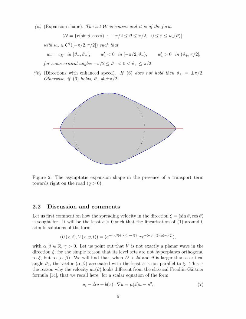
(ii) (Expansion shape). The set W is convex and it is of the form

W = r(sinϑ, cosϑ) : −π/2 ≤ ϑ ≤ π/2, 0 ≤ r ≤ w∗(ϑ),

with w∗ ∈ C1([−π/2, π/2]) such that

w∗ = cK in [ϑ−, ϑ+], w′∗ < 0 in [−π/2, ϑ−), w′∗ > 0 in (ϑ+, π/2],

for some critical angles −π/2 ≤ ϑ− < 0 < ϑ+ ≤ π/2.

(iii) (Directions with enhanced speed). If (6) does not hold then ϑ± = ±π/2.Otherwise, if (6) holds, ϑ± 6= ±π/2.

Figure 2: The asymptotic expansion shape in the presence of a transport termtowards right on the road (q > 0).

2.2 Discussion and comments

Let us first comment on how the spreading velocity in the direction ξ = (sinϑ, cosϑ)is sought for. It will be the least c > 0 such that the linearisation of (1) around 0admits solutions of the form

(U(x, t), V (x, y, t)) = (e−(α,β)·((x,0)−ctξ), γe−(α,β)·((x,y)−ctξ)),

with α, β ∈ R, γ > 0. Let us point out that V is not exactly a planar wave in thedirection ξ, for the simple reason that its level sets are not hyperplanes orthogonalto ξ, but to (α, β). We will find that, when D > 2d and ϑ is larger than a criticalangle ϑ0, the vector (α, β) associated with the least c is not parallel to ξ. This isthe reason why the velocity w∗(ϑ) looks different from the classical Freidlin-Gartnerformula [14], that we recall here: for a scalar equation of the form

ut −∆u+ b(x) · ∇u = µ(x)u− u2, (7)

6

with µ > 0, µ and b 1-periodic, the spreading velocity in the direction ξ is given by

w∗(ξ) = infξ·ξ′>0

c∗(ξ)

ξ · ξ′(8)

where c∗(ξ) is the least c such that the linearisation of (7) around 0:

ut −∆u+ b(x) · ∇u = µ(x)u, (9)

admits solutions of the form

φ(x)eλ(x·ξ−ct), φ > 0, 1-periodic.

The optimal assumption for µ is not, by the way, µ > 0. A more general assumptionis λper1 (−∆ − µ(x)) < 0, where λper1 denotes the first periodic eigenvalue. In anycase, (8) gives the formula

∀ξ, ξ′ ∈ RN\0, c∗(ξ) ≥ w∗(ξ)ξ · ξ′.

We will see in Section 6 (Lemma 6.1 below) that a similar, but different, formulaholds in our case, namely,

∀ϑ ∈ [ϑ0, π/2], ϑ ∈ [0, π/2], w∗(ϑ) ≤ cos(ϑ− ϕ∗(ϑ))

cos(ϑ− ϕ∗(ϑ))w∗(ϑ).

It will, in fact, be derived as a consequence of the expression of the spreading velocity.Several proofs of the Freidlin-Gartner formula have been given, besides that

of [14]. See Evans-Souganidis [12] for a viscosity solutions/singular perturbations ap-proach, Weinberger [17] for an abstract monotone system proof; Berestycki-Hamel-Nadin [4] for a PDE proof. See also [5] for equivalent formulae and estimates of thespreading speed in periodic media, as well as [8] for one-dimensional general media.Many of these results are explained, and developped, in [3].

Let us now discuss the shape of the set W in Theorem 2.1, and how it comparesto W . The latter has a very natural interpretation as the reachable set from theorigin in time 1 by moving with speed c∗ on the road and cK in the field. Indeed,considering trajectories obtained by moving on the road until time λ ∈ [0, 1] andthen on a straight line in the field for the remaining time 1− λ, one finds that thereachable set is the convex hull of the union of the segment [−c∗, c∗]× 0 and thehalf-disc BcK ∩ Ω, that is, W .

Another way to obtain the set W is the following: consider a set-valued mapt 7→ Ut ∈ Ω and impose that the trace of Ut expands at speed c∗ on the x-axis, andthat the rest evolves by asking that the normal velocity of its boundary equals cK .In PDE terms, Ut = (x, y) : φ(x, y, t) ≥ 1, where φ solves the eikonal equation

φt − cK |∇φ| = 0 t > 0, (x, y) ∈ Ω

φ(x, 0, t) = 1[−c∗t,c∗t](x) t > 0, x ∈ R

So, the family of sets (Ut)t>0 is simply obtained by applying the Huygens principlewith the segment [−c∗t, c∗t] on the road as a source. In other words, tW = Ut and it

7

evolves with normal velocity cK . Notice that imposing that a family of sets (tA)t>0

evolves with normal velocity cK forces the curvature of A to be either 1/cK or 0,i.e.,A is locally either a disc of radius cK or a half-plane. It would have been temptingto think that W coincides with W , just as in the singular perturbation approachto front propagation in parabolic equations or systems - see Evans-Souganidis [12],[13]. The fact that the asymptotic expansion shape is actually larger than this setis remarkable. And, as a matter of fact, we estimate in Proposition 6.4 below thedifference between W and W in terms of the normal velocities of their boundarieswhen magnified by t. Namely, we discover that the normal speed of (tW)t>0 at aboundary point t(sinϑ, cosϑ), ϑ > ϑ0, coincides with the normal speed of the levellines of the planar wave for the linearised system which defines w∗(ϑ) - see the nextsection. This speed is larger than cK because the exponential decay rate of V inthe direction orthogonal to its level lines is less than the critical one:

√f ′(0)/d.

We expect this decay to be approximatively satisfied for large time by the solutionof (1) emerging from a compactly supported initial datum. Thus, heuristically, thepresence of the road would result in an “unnatural” decay for solutions of the KPPequation with compactly supported initial data, which, in turns, would be the reasonwhy W does not coincide with the set W following from Huygens’ principle.

3 Planar waves for the linearised system

Consider the linearisation of system (1) around v = 0:∂tu−D∂xxu = νv|y=0 − µu x ∈ R, t > 0

∂tv − d∆v = f ′(0)v (x, y) ∈ Ω, t > 0

−d∂yv|y=0 = µu(x, t)− νv|y=0 x ∈ R, t > 0.

(10)

Take a unit vector ξ = (ξ1, ξ2), with ξ2 ≥ 0. By symmetry, we restrict to ξ1 ≥ 0. Assaid above, solutions are sought for in the form

(U(x, t), V (x, y, t)) = (e−(α,β)·((x,0)−ctξ), γe−(α,β)·((x,y)−ctξ)), (11)

with c ≥ 0, γ > 0 and α, β ∈ R (not necessarily positive). This leads to the systemc ξ · (α, β)−Dα2 = νγ − µc ξ · (α, β)− d(α2 + β2) = f ′(0)

dγβ = µ− νγ.

The third equation yields γ = µ/(ν + dβ) and then β > −ν/d. Setting χ(s) :=µs/(ν + s), the system on (α, β) reads

cξ1α + cξ2β −Dα2 = −χ(dβ)

cξ1α + cξ2β − d(α2 + β2) = f ′(0).(12)

The first equation in the unknown α has the roots

α±D(c, β) :=1

2D

(cξ1 ±

√(cξ1)2 + 4D (cξ2β + χ(dβ))

),

8

which are real if and only if β is larger than some value β(c) ∈ (−ν/d, 0]. The set ofreal solutions (β, α) of the first equation in (12) is then Σ(c) = Σ−(c)∪Σ+(c), with

Σ±(c) := (β, α±D(c, β)) : β ≥ β(c).

This is a smooth curve with leftmost point (β(c), cξ1/2D). Rewriting the second

equation in (12) as |(α, β)− c

2dξ|2 =

c2

4d2− f ′(0)

d, we see that it has solution if and

only if c ≥ cK , where cK := 2√df ′(0) is the invasion speed in the field. In the (β, α)

plane, it represents the circle Γ(c) of centre C(c) and radius r(c) given by

C(c) =c

2d(ξ2, ξ1), r(c) =

√c2 − c2K

2d.

Let S(c) denote the closed set bounded from below by Σ−(c) and from above byΣ+(c) and let G(c) denote the closed disc with boundary Γ(c). Exponential functionsof the type (11) are supersolutions of (10) if and only if (β, α) ∈ S(c) ∩ G(c). Sincethe centre C(c) belongs to the line s 7→ s(ξ2, ξ1) and the closest point of Γ(c) to theorigin, P (c) := C(c)− r(c)(ξ2, ξ1), satisfies

P ′(c) · (ξ2, ξ1) =1

2d− c

d√c2 − c2K

< 0, limc→+∞

P (c) = 0,

we find that

∀c′ ≥ c ≥ cK , G(c′) ⊃ G(c),⋃c≥cK

G(c) = (β, α) : (β, α) · (ξ2, ξ1) > 0.

On the other hand, α+D(c, β) is increasing in c and concave in β, the latter following

from the concavity of cξ2β + χ(dβ).Therefore, there exists w∗ ≥ cK , depending on ξ, such that

S(c) ∩ G(c) 6= ∅ ⇔ c ≥ w∗,

with S(w∗) ∩ G(w∗) consisting in a singleton, denoted by (β∗, α∗), see Figures 3and 4. Moreover, w∗ = cK if and only if C(cK) ∈ S(cK), namely, if and only ifC(cK) satisfies the first condition in (12) with = replaced by ≥ :

c2K2d− Dc2K

4d2ξ21 ≥ −

µcKξ22ν + cKξ2

.

Since ξ21 = 1− ξ22 , this inequality rewrites

2d+D(ξ22 − 1) +4d2µξ2

2νcK + c2Kξ2≥ 0.

The function Φ : [0,+∞)→ R defined by

Φ(s) := 2d+D(s2 − 1) +4d2µs

2νcK + c2Ks,

9

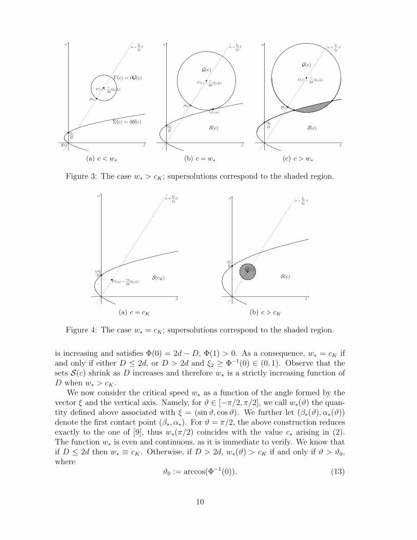
(a) c < w∗ (b) c = w∗ (c) c > w∗

Figure 3: The case w∗ > cK ; supersolutions correspond to the shaded region.

(a) c = cK (b) c > cK

Figure 4: The case w∗ = cK ; supersolutions correspond to the shaded region.

is increasing and satisfies Φ(0) = 2d −D, Φ(1) > 0. As a consequence, w∗ = cK ifand only if either D ≤ 2d, or D > 2d and ξ2 ≥ Φ−1(0) ∈ (0, 1). Observe that thesets S(c) shrink as D increases and therefore w∗ is a strictly increasing function ofD when w∗ > cK .

We now consider the critical speed w∗ as a function of the angle formed by thevector ξ and the vertical axis. Namely, for ϑ ∈ [−π/2, π/2], we call w∗(ϑ) the quan-tity defined above associated with ξ = (sinϑ, cosϑ). We further let (β∗(ϑ), α∗(ϑ))denote the first contact point (β∗, α∗). For ϑ = π/2, the above construction reducesexactly to the one of [9], thus w∗(π/2) coincides with the value c∗ arising in (2).The function w∗ is even and continuous, as it is immediate to verify. We know thatif D ≤ 2d then w∗ ≡ cK . Otherwise, if D > 2d, w∗(ϑ) > cK if and only if ϑ > ϑ0,where

ϑ0 := arccos(Φ−1(0)). (13)

10

Notice that ϑ0 is a decreasing function of D. We finally define

W := r(sinϑ, cosϑ) : −π/2 ≤ ϑ ≤ π/2, 0 ≤ r ≤ w∗(ϑ).

The object of Sections 4 and 5 is to show that W is the asymptotic expansion setfor (1).

4 Compactly supported subsolutions

This section is dedicated to the construction, for all ϑ ∈ (−π/2, π/2), of compactlysupported subsolutions moving in the direction ξ = (sinϑ, cosϑ) with speed lessthan, but arbitrarily close to, w∗(ϑ). We derive the following

Lemma 4.1. For all ϑ ∈ (−π/2, π/2) and ε > 0, there exist c > w∗(ϑ) − ε and apair (u, v) of nonnegative functions with the following properties: u|t=0 and v|t=0 arecompactly supported,

∃(x, y) ∈ Ω, ∀t ≥ 0, v(x+ ct sinϑ, y + ct cosϑ, t) = v(x, y, 0) > 0, (14)

and κ(u, v) is a generalised subsolution of (1) for all κ ∈ (0, 1].

By symmetry, it is sufficient to prove the lemma for ϑ ≥ 0. The case ϑ = π/2 wastreated in [9]. If ϑ ∈ [0, ϑ0] then w∗(ϑ) = cK and the construction is standard, aswe will see in Section 4.2. In Section 4.3 we treat the remaining cases by exploitingthe analysis of planar waves performed in the previous section. We will proceed asfollows:

1. We first give a definition of generalised subsolutions adapted to our context.

2. For c ∈ (0, w∗(ϑ)) close enough to w∗(ϑ), we apply Rouche’s theorem to provethe existence of a complex exponential solution (U, V ) of the linearised system,which moves in the direction ξ = (sinϑ, cosϑ) with speed c. We actually workon a perturbed system in order to get strict subsolutions of the nonlinear one.

3. The connected components of the positivity set of u := ReU are boundedintervals and those of v := ReV are infinite strips. In order to truncate thosestrips, we consider the reflection vL of v with respect to the line (x, y) · ξ⊥ =L > 0. We then define the pair (u, v) by setting (u, v) = (u, v − vL) in aconnected component of the positivity sets of u and v − vL, (0, 0) outside.

4. The function v is automatically a generalised subsolution of the equation inthe field. We show that, choosing L large enough, (u, v) is a generalisedsubsolution of the equations on the road too.

11

4.1 Sub/supersolutions

In the sequel, we will need to compare the solution of the Cauchy problem with apair (u, v) which is a subsolution inside some regions, vanishes on their boundaries,and is truncated to 0 outside. In the case of a single equation, such type of functionsare generalised subsolutions, in the sense that they satisfy the comparison principlewith supersolutions. This kind of properties has the flavour of those presented in [7].In the case of a system, this property may not hold because, roughly speaking, onecould truncate one component in a region where it is needed for the others to besubsolutions. This is why we need a different notion of generalised subsolution.

We consider pairs (u, v) such that u is the maximum of subsolutions of the firstequation in (1) with v = v, while v is the maximum of subsolutions of the secondequation and of the last equation with u = u. More precisely:

Definition 4.2. A pair (u, v) is a generalised subsolution of (1) if u, v are continuousand satisfy the following properties:

(i) for any x ∈ R, t > 0, there is a function u such that u ≤ u in a neighbourhoodof (x, t) and, at (x, t) (in the classical sense),

u = u, ∂tu−D∂xxu+ µu ≤ νv|y=0 ;

(ii) for any (x, y) ∈ Ω, t > 0, there is a function v such that v ≤ v in a neighbour-hood of (x, y, t) and, at (x, y, t),

v = v, ∂tv − d∆v ≤ f(v) if y > 0, −d∂yv + νv ≤ µu if y = 0.

Although this will not be needed in the paper, we may define generalised super-solutions in analogous way, by replacing “≤” with “≥” everywhere in Definition 4.2.This notion is stronger than that of viscosity solution (see, e.g., [11]). Nevertheless,it recovers: (i) classical subsolutions, (ii) maxima of classical subsolutions and (iii)generalised subsolutions in the sense of [9]. From now on, generalised sub and su-persolutions are understood in the sense of Definition 4.2. The comparison principlereads:

Proposition 4.3. Let (u, v) and (u, v) be respectively a generalised subsolutionbounded from above and a generalised supersolution bounded from below of (1) suchthat (u, v) is below (u, v) at time t = 0. Then (u, v) is below (u, v) for all t > 0.

The proof is similar to the one of Proposition 3.3 in [9], even if the notion of suband supersolution is slightly more general here. It is included here in Appendix 7for the sake of completeness.

4.2 The case ϑ ≤ ϑ0

Let λ(R) and ϕ be the principal eigenvalue and eigenfunction of the operator −d∆−c(sinϑ, cosϑ) ·∇ in the two dimensional ball BR, with Dirichlet boundary condition.

12

This operator can be reduced to a self-adjoint one by multiplying the functions timese(sinϑ,cosϑ)·(x,y)c/2d. One then finds that (λ(R) − c2/4d)/d is equal to the principaleigenvalue of −∆ in BR. Whence, for 0 < c < w∗(ϑ) = cK ,

limR→∞

λ(R) =c2

4d< f ′(0).

There is then R > 0 such that f(s) ≥ λ(R)s for s > 0 small enough, and thereforewe can normalise the principal eigenfunction ϕ in such a way that

∀κ ∈ [0, 1], −d∆(κϕ)− c(sinϑ, cosϑ) · ∇(κϕ) ≤ f(κϕ) in BR.

It follows that the pair (u, v) defined by u ≡ 0,

v(x, y, t) =

ϕ(x− ct sinϑ, y −R− ct cosϑ) if (x, y −R)− ct(sinϑ, cosϑ) ∈ BR

0 otherwise

satisfies the properties stated in Lemma 4.1.

4.3 The case ϑ > ϑ0

Suppose now that D > 2d and consider ϑ ∈ (ϑ0, π/2). Call

ξ := (sinϑ, cosϑ), ξ⊥ := (− cosϑ, sinϑ),

and, to ease notation, w∗ = w∗(ϑ), α∗ = α∗(ϑ), β∗ = β∗(ϑ).

4.3.1 Complex exponential solutions for the penalised system

We start with the following

Lemma 4.4. For c ∈ (0, w∗) close enough to w∗, (10) admits an exponential solution(U, V ) of the type (11) with α, β, γ ∈ C\R satisfying

Reα,Re β > 0, 0 <Imα

Im β<

Reα

Re β<ξ1ξ2. (15)

Proof. For c < w∗, problem (10) does not admit exponential solutions of the type(11), with α, β, γ ∈ R. However, if w∗− c is small enough, applying the Rouche the-orem to the distance between Γ and Σ as a function of β, one obtains an exponentialsolution (U, V ) with α, β, γ ∈ C, depending on c, and satisfying

α = αr + iαi, β = βr + iβi, γ =µ

ν + dβ,

βr = β∗ +O(w∗ − c), 0 6= βi = O(√w∗ − c).

See the proof of Lemma 6.1 in [9] for the details. Writing separately the real andcomplex terms of the second equation of the system (12) satisfied by α, β, we get

cξ · (αr, βr)− d(α2r − α2

i + β2r − β2

i ) = f ′(0)

cξ · (αi, βi)− 2d(αrαi + βrβi) = 0.(16)

13

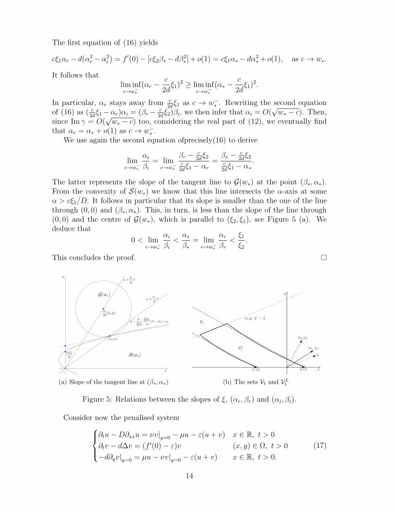
The first equation of (16) yields

cξ1αr − d(α2r −α2

i ) = f ′(0)− [cξ2β∗− dβ2∗ ] + o(1) = cξ1α∗− dα2

∗+ o(1), as c→ w∗.

It follows thatlim infc→w−∗

(αr −c

2dξ1)

2 ≥ lim infc→w−∗

(α∗ −c

2dξ1)

2.

In particular, αr stays away from c2dξ1 as c → w−∗ . Rewriting the second equation

of (16) as ( c2dξ1−αr)αi = (βr− c

2dξ2)βi, we then infer that αi = O(

√w∗ − c). Then,

since Im γ = O(√w∗ − c) too, considering the real part of (12), we eventually find

that αr = α∗ + o(1) as c→ w−∗ .We use again the second equation ofprecisely(16) to derive

limc→w−∗

αiβi

= limc→w−∗

βr − c2dξ2

c2dξ1 − αr

=β∗ − c

2dξ2

c2dξ1 − α∗

.

The latter represents the slope of the tangent line to G(w∗) at the point (β∗, α∗).From the convexity of S(w∗) we know that this line intersects the α-axis at someα > cξ1/D. It follows in particular that its slope is smaller than the one of the linethrough (0, 0) and (β∗, α∗). This, in turn, is less than the slope of the line through(0, 0) and the centre of G(w∗), which is parallel to (ξ2, ξ1), see Figure 5 (a). Wededuce that

0 < limc→w−∗

αiβi<α∗β∗

= limc→w−∗

αrβr

<ξ1ξ2.

This concludes the proof.

(a) Slope of the tangent line at (β∗, α∗) (b) The sets Vt and VLt

Figure 5: Relations between the slopes of ξ, (αr, βr) and (αi, βi).

Consider now the penalised system∂tu−D∂xxu = νv|y=0 − µu− ε(u+ v) x ∈ R, t > 0

∂tv − d∆v = (f ′(0)− ε)v (x, y) ∈ Ω, t > 0

−d∂yv|y=0 = µu− νv|y=0 − ε(u+ v) x ∈ R, t > 0.

(17)

14

A small perturbation ε does not affect the qualitative results of Section 3 1 northat of Lemma 4.4. Thus, for ε small enough, there exists wε∗ such that (17) admitsexponential solutions in the form (11) with α, β, γ ∈ R for c ≥ wε∗, and with α, β, γ ∈C\R satisfying (15) for c < wε∗ close enough to wε∗. Moreover, wε∗ → w∗ as ε→ 0. Weare interested in the complex ones. Until the end of Section 4, (U, V ) will denote anexponential solution of (17), with ε > 0 sufficiently small, α, β, γ ∈ C\R satisfying(15) and c < wε∗ close to wε∗. Changing the sign to the imaginary part of both Uand V we still have a solution. Hence, by (15), it is not restrictive to assume thatImα, Im β > 0.

We set for short αr := Reα, αi := Imα, βr := Re β, βi := Im β. Since γ−1 =(ν+ε+dβ)/(µ−ε) by the last equation of (17), it follows that Arg (γ−1) ∈ (0, π/2).Resuming, we have:

αr, αi, βr, βi > 0,αiβi<αrβr

<ξ1ξ2, Arg (γ−1) ∈ (0, π/2). (18)

4.3.2 Truncating the exponential solution and the equation in the field

The pair (u, v) defined by

u := ReU = e−(αr,βr)·[(x,0)−ctξ] cos((αi, βi) · [(x, 0)− ctξ]),

v := ReV = |γ|e−(αr,βr)·[(x,y)−ctξ] cos((αi, βi) · [(x, y)− ctξ]− Arg γ),

is a real solution of (17). Consider the following connected components of thepositivity sets of u, v at time 0:

U =

(− π

2αi,π

2αi

), V := (x, y) ∈ R2 : (αi, βi)·(x, y) ∈ (−π

2+Arg γ,

π

2+Arg γ).

As the time t increases, these connected components are shifted, becoming

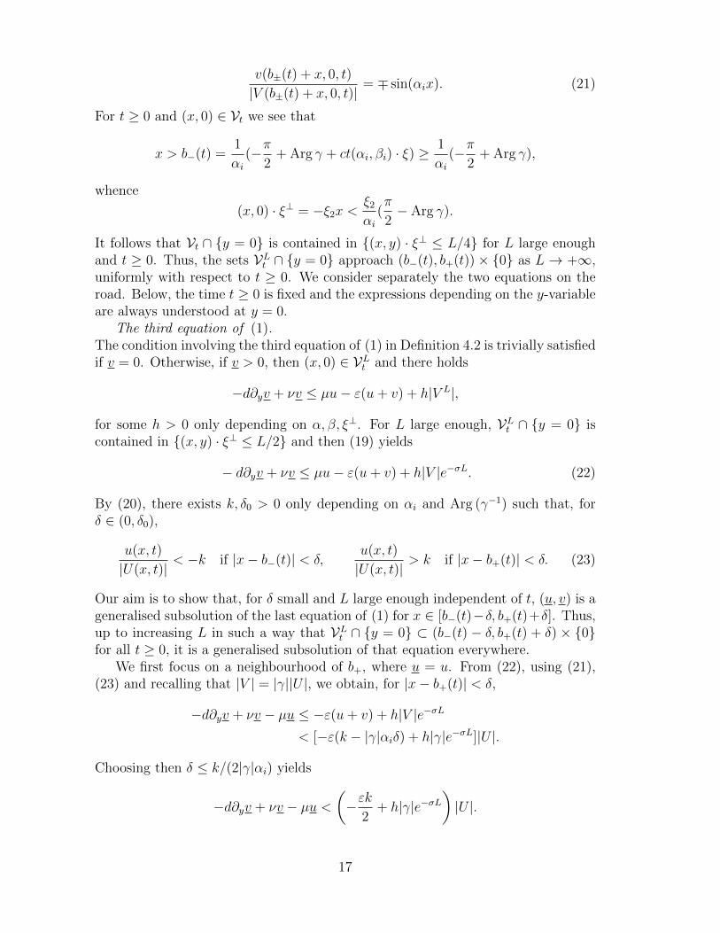
Ut := U + ctξ1 +βiαiξ2, Vt := V + ctξ.

In order to truncate the sets Vt we consider the reflection with respect to the line(x, y) · ξ⊥ = L, with L > 0, where, we recall, ξ⊥ := (− cosϑ, sinϑ). Namely

RL(x, y) = (x, y) + 2(L− (x, y) · ξ⊥)ξ⊥.

We then define

V L(x, y, t) := V (RL(x, y), t), vL := ReV L.

The function v − vL vanishes on (x, y) · ξ⊥ = L and satisfies the second equationof (17). The quotient |V L|/|V | satisfies

|V L||V |

=e−(αr,βr)·[R

L(x,y)−ctξ]

e−(αr,βr)·[(x,y)−ctξ]= e−2(αr,βr)·ξ

⊥(L−(x,y)·ξ⊥).

1 the curves Σ,Γ are replaced by some curves converging locally uniformly to Σ,Γ as ε → 0,together with their derivatives

15

Let us call σ := (αr, βr) · ξ⊥. It follows from (18) that σ > 0. Hence,

|V L||V |≤ 1 if (x, y) · ξ⊥ ≤ L,

|V L||V |≤ e−σL if (x, y) · ξ⊥ ≤ L

2. (19)

We deduce that, when restricted to the half-plane (x, y) · ξ⊥ ≤ L/2, a connectedcomponent of the set where (v− vL) is positive at time t, denoted by VLt , convergesin Hausdorff distance to Vt as L→∞, uniformly in t ≥ 0. We can now define

u(x, t) :=

u(x, t) if x ∈ Ut0 otherwise,

v(x, y, t) :=

(v − vL)(x, y, t) if (x, y) ∈ VLt0 otherwise.

We claim that v is bounded. The set VLt satisfies

VLt ⊂ (x, y) · ξ⊥ ≤ L ∩ −π + Arg γ ≤ (αi, βi) · [(x, y)− ctξ] ≤ π + Arg γ,

as it is seen by noticing that v = −|V | on the boundary of the latter set and|vL| ≤ |V | if (x, y) · ξ⊥ ≤ L. Thus

v ≤ 2|γ| sup(x,y)·ξ⊥≤L

[(x,y)−ctξ]·(αi,βi)≥−π+Arg γ

e−(αr,βr)·[(x,y)−ctξ] = 2|γ| sup(x,y)·ξ⊥≤L

(x,y)·(αi,βi)≥−π+Arg γ

e−(αr,βr)·(x,y).

It follows from geometrical considerations that the latter supremum is finite, c.f. Fig-ure 5 (b). Analytically, one sees that it is finite if and only if

(x, y) · (−ξ⊥) ≥ 0 ∩ (x, y) · (αi, βi) ≥ 0 ⊂ (x, y) · (αr, βr) ≥ 0,

which is equivalent to require that (αr, βr) = λ1(−ξ⊥) + λ2(αi, βi) with λ1, λ2 ≥0. This property holds true by (18). We therefore have that (u, v) is bounded.Furthermore, v is a generalized subsolution of the second equation of (17). Sincef(s) ≥ (f ′(0) − ε)s for s > 0 small enough, we can renormalise (u, v) in such away that κv is a generalized subsolution of the second equation of (1) too, for allκ ∈ [0, 1]. Next, like v, vL satisfies vL((x, y)+ctξ, t) = vL(x, y, 0) and thus (14) holds.It only remains to show that (u, v) is a generalized subsolution of the equations onthe road in the sense of Definition 4.2.

4.3.3 The equations on the road

Let us write

Ut = (a−(t), a+(t)), Vt ∩ y = 0 = (b−(t), b+(t))× 0.

Since Arg (γ−1) ∈ (0, π/2) by (18), we deduce that

b−(t) = a−(t)−Arg (γ−1)

αi< a−(t) < b−(t)+

π

αi= b+(t) = a+(t)−Arg (γ−1)

αi< a+(t).

We further see that

u(b±(t) + x, t)

|U(b±(t) + x, t)|= ± sin(−αix+ Arg (γ−1)). (20)

16

v(b±(t) + x, 0, t)

|V (b±(t) + x, 0, t)|= ∓ sin(αix). (21)

For t ≥ 0 and (x, 0) ∈ Vt we see that

x > b−(t) =1

αi(−π

2+ Arg γ + ct(αi, βi) · ξ) ≥

1

αi(−π

2+ Arg γ),

whence

(x, 0) · ξ⊥ = −ξ2x <ξ2αi

(π

2− Arg γ).

It follows that Vt ∩ y = 0 is contained in (x, y) · ξ⊥ ≤ L/4 for L large enoughand t ≥ 0. Thus, the sets VLt ∩ y = 0 approach (b−(t), b+(t))× 0 as L→ +∞,uniformly with respect to t ≥ 0. We consider separately the two equations on theroad. Below, the time t ≥ 0 is fixed and the expressions depending on the y-variableare always understood at y = 0.

The third equation of (1).The condition involving the third equation of (1) in Definition 4.2 is trivially satisfiedif v = 0. Otherwise, if v > 0, then (x, 0) ∈ VLt and there holds

−d∂yv + νv ≤ µu− ε(u+ v) + h|V L|,

for some h > 0 only depending on α, β, ξ⊥. For L large enough, VLt ∩ y = 0 iscontained in (x, y) · ξ⊥ ≤ L/2 and then (19) yields

− d∂yv + νv ≤ µu− ε(u+ v) + h|V |e−σL. (22)

By (20), there exists k, δ0 > 0 only depending on αi and Arg (γ−1) such that, forδ ∈ (0, δ0),

u(x, t)

|U(x, t)|< −k if |x− b−(t)| < δ,

u(x, t)

|U(x, t)|> k if |x− b+(t)| < δ. (23)

Our aim is to show that, for δ small and L large enough independent of t, (u, v) is ageneralised subsolution of the last equation of (1) for x ∈ [b−(t)−δ, b+(t)+δ]. Thus,up to increasing L in such a way that VLt ∩ y = 0 ⊂ (b−(t) − δ, b+(t) + δ) × 0for all t ≥ 0, it is a generalised subsolution of that equation everywhere.

We first focus on a neighbourhood of b+, where u = u. From (22), using (21),(23) and recalling that |V | = |γ||U |, we obtain, for |x− b+(t)| < δ,

−d∂yv + νv − µu ≤ −ε(u+ v) + h|V |e−σL

< [−ε(k − |γ|αiδ) + h|γ|e−σL]|U |.

Choosing then δ ≤ k/(2|γ|αi) yields

−d∂yv + νv − µu <(−εk

2+ h|γ|e−σL

)|U |.

17

We eventually infer that, for L large enough independent of t, (u, v) is a generalisedsubsolution of the last equation of (1) in the δ neighbourhood of b+(t). Considernow points such that |x− b−(t)| < δ, where u = 0. By (22) we get

−d∂yv + νv − µu ≤ (µ− ε)u− εv + h|V |e−σL

< [−(µ− ε)k + ε|γ|αiδ + h|γ|e−σL]|U |,

provided that ε < µ. Taking ε < µ/2 we end up with the same inequality as in thecase |x−b+(t)| < δ treated above. It remains the case x ∈ [b−(t)+δ, b+(t)−δ]. Therewe have that v ≥ k′|V |, for some k′ > 0 only depending on αi, δ. Consequently,using the fact that u = max(u, 0), we obtain

−d∂yv + νv ≤ (µ− ε)u− εv + h|V |e−σL

≤ µu− (εk′ − he−σL)|V |.

We get again a subsolution for L large enough.The second equation of (1).

The non-trivial case is x ∈ Ut = (a−(t), a+(t)), where

∂tu+ µu− νv = (ν − ε)v − εu− νv.

If x ∈ [b+(t), a+(t)) then ∂tu + µu − νv ≤ 0, provided that ε ≤ ν. As before,let k, δ0 > 0 be such that (23) holds for δ ∈ (0, δ0). Using (21) and the equality|V | = |γ||U | we get, if |x− b+(t)| < δ,

∂tu+ µu− νv ≤ [|ν − ε||γ|αiδ − εk]|U |,

which is negative for δ small, independent of t. Consider the remaining case x ∈(a−(t), b+(t)−δ]. There, from one hand v ≥ k′|V | with k′ only depending on αi, γ, δ,from the other, by (19), vL ≤ |V |e−σL provided that L is large enough in such a waythat −a−(t) cosϑ ≤ L/2. Hence,

∂tu+ µu− νv = νvL − εv − εu ≤ (νe−σL − εk′)|V |.

We eventually infer that, for L large enough independent of t, (u, v) is a generalisedsubsolution of the second equation of (1). This concludes the proof of Lemma 4.1.

5 Proof of the spreading property

In this section we show that the setW defined in Section 3 is indeed the asymptoticexpansion shape of the system (1). This proves Theorem 2.1 part (i). Moreover, bythe definition of the critical angle ϑ0, part (iii) also follows.

We show separately that solutions spread at most and at least with the velocitysetW , c.f. (3) and (4) respectively. The upper bound (3) follows by comparison withthe planar waves of Section 3. The proof of (4) is more involved. It combines the

18

convergence result close to the road given by [9] with the existence of compactly sup-ported subsolutions provided by Lemma 4.1. Then one concludes using a standardLiouville-type result for strictly positive solutions.

Throughout this section, (u, v) denotes a solution of (1) with an initial datum(u0, v0) 6≡ (0, 0) compactly supported. As already mentioned in the introduction,the well-posedness of the Cauchy problem is proved in [9].

5.1 The upper bound

Proof of (3). We prove (3) showing that, for any ε > 0, there exists T > 0 suchthat the following holds:

∀ϑ ∈ [−π/2, π/2], c ≥ w∗(ϑ) + ε, t ≥ T, v(ct sinϑ, ct cosϑ, t) < ε.

By symmetry, we can restrict ourselves to ϑ ∈ [0, π/2]. Let R > 0 be such that

suppu0 ⊂ [−R,R], supp v0 ⊂ BR.

For ϑ ∈ [−π/2, π/2], let (Uϑ, Vϑ) be the planar wave for the linearised system (10)defined by (11) with ξ = (sinϑ, cosϑ), c = w∗(ϑ), α = α∗(ϑ), β = β∗(ϑ) andγ = µ/(ν + dβ∗(ϑ)). It is straightforward to check that the functions α∗ and β∗ arecontinuous, hence bounded. Since for ϑ ∈ [0, π/2] it holds that

∀(x, y) ∈ BR, Uϑ(x, 0) ≥ e−|R|α∗(ϑ), Vϑ(x, y, 0) ≥ µ

ν + dβ∗(ϑ)e−|R|(α∗(ϑ),β∗(ϑ)),

there exists κ > 0, independent of ϑ, such that all the κ(Uϑ, Vϑ) are above (u, v) attime 0. The pairs κ(Uϑ, Vϑ) are still supersolutions of (10), and then of (1) because,by the KPP hypothesis, f ′(0)κVϑ ≥ f(κVϑ). The comparison principle then yieldsthat, for ϑ ∈ [0, π/2] and t ≥ 0, κVϑ ≥ v, whence, in particular,

∀c ≥ 0, v(ct sinϑ, ct cosϑ, t) ≤ κµ

ν + dβ∗(ϑ)e−(c−w∗(ϑ))t(α∗(ϑ),β∗(ϑ))·(sinϑ,cosϑ).

Notice now that the functions α∗ and β∗ are strictly positive, excepted at 0 whereα∗ = 0, β∗ 6= 0, and at π/2 where α∗ 6= 0, β∗ = 0 if D ≤ 2d. It follows that(α∗(ϑ), β∗(ϑ)) · (sinϑ, cosϑ) is positive on [0, π/2], thus it has a positive minimumby continuity. The result then follows.

5.2 The lower bound

Proof of (4). We first show that v is bounded from below away from 0 in somesuitable expanding sets. This allows us to conclude by means of a standard Liouville-type result for entire solutions with positive infimum.

Step 1. For ε ∈ (0, cK) and ϑ ∈ [−π/2, π/2], there exist (x, y) ∈ Ω and an openset A in the relative topology of Ω such that

A ⊃ r(sinϑ, cosϑ) : 0 ≤ r ≤ w∗(ϑ)− ε, inft≥1

(x,y)∈tA

v(x+ x, y + y, t) > 0.

19

Consider the case ϑ 6= ±π/2. Let (u, v) be a generalised subsolution given by Lemma4.1, with c > w∗(ϑ)− ε > 0, and set

δ :=c− w∗(ϑ) + ε

2c∈ (0, 1/2).

Even if it means multiplying u, v by a small factor κ > 0, we can assume thatsup u|t=0 < ν/µ, sup v|t=0 < 1. We now make use of the spreading result from[9], summarized here by (2). Recalling that the c∗ there coincides with w∗(π/2),the second limit implies the existence of τ > 0 such that, for λ ∈ (δ, 1] and |c′| <w∗(π/2)− ε/2, the following holds true:

∀(x, y) ∈ Ω, t ≥ τ, v(x+ c′λt, y, λt) > v(x, y, 0), u(x+ c′λt, λt) > u(x, 0).

Then, by comparison, v(x + c′λt, y, λt + s) ≥ v(x, y, s) for t ≥ τ and s ≥ 0, fromwhich, taking s = (1− λ)t and (x, y) = (x, y) + c(1 − λ)t(sinϑ, cosϑ), where (x, y)is such that (14) holds, we get

v(x+ [c(1− λ) sinϑ+ c′λ]t, y + [c(1− λ) cosϑ]t, t) > v(x, y, 0) > 0.

Namely,inft≥τ

(x,y)∈tA

v(x+ x, y + y, t) > 0,

where A is the following set:

A = (c(1− λ) sinϑ+ c′λ, c(1− λ) cosϑ) : δ < λ ≤ 1, |c′| < w∗(π/2)− ε/2,

which is open in the relative topology of Ω. By the choice of δ, restricting to thevalues c′ = 0 and 2δ ≤ λ ≤ 1 in the expression of A we recover the segmentr(sinϑ, cosϑ) : 0 ≤ r ≤ w∗(ϑ) − ε. While, restricting to λ = 1 and |c′| ≤w∗(π/2)−ε, we obtain [−w∗(π/2)+ε, w∗(π/2)−ε]×0, which is the sought segmentin the case ϑ = ±π/2. The proof of the step 1 is thereby complete, because theminimum of v on compact subsets of Ω× [1, τ ] is positive by the strong comparisonprinciple with (0, 0).

Step 2. Conclusion.Fix ε ∈ (0, cK). Let ((xn, yn))n∈N be a sequence in Ω and (tn)n∈N a sequence in R+

such that

limn→∞

tn = +∞, ∀n ∈ N, dist

(1

tn(xn, yn),Ω\W

)> ε.

By the boundedness of v it follows that (v(xn, yn, tn))n∈N converges up to subse-quences. In order to prove (4) we need to show that the limits of all convergingsubsequences are equal to 1. Let us still call (v(xn, yn, tn))n∈N one of such subse-quences and set

m := limn→∞

v(xn, yn, tn).

20

If (yn)n∈N admits a bounded subsequence (ynk)k∈N then, since

ε < dist

(1

tnk(xnk , ynk),Ω\W

)≤ dist

(xnktnk

,R\[−w∗(π/2), w∗(π/2)]

)+ynktnk

,

we derive |xnk | ≤ (w∗(π/2) − ε/2)tnk for k large enough. It then follows from (2)that m = 1 in this case. Consider now the case where (yn)n∈N diverges. Let us write1/tn(xn, yn) = rn(sinϑn, cosϑn), with |ϑn| ≤ π/2 and 0 ≤ rn ≤ w∗(ϑn)− ε, and callϑ, r the limit of (a subsequence of) (ϑn)n∈N, (rn)n∈N respectively. The continuity ofw∗ yields 0 ≤ r ≤ w∗(ϑ)− ε. Consider the sequence of functions (vn)n∈N defined by

vn(x, y, t) := v(x+ xn, y + yn, t+ tn).

For n large enough, the vn are defined in any given K ⊂⊂ R2 × R and, by interiorparabolic estimates (see, e.g., [16]) they are uniformly bounded in C2,δ(K) andC1,δ(K) with respect to the space and time variables respectively, for some δ ∈ (0, 1).Hence, (vn)n∈N converges (up to subsequences) locally uniformly to a solution v∞ of

∂tv∞ − d∆v∞ = f(v∞), (x, y) ∈ R2, t ∈ R. (24)

Moreover, v∞(0, 0, 0) = m. Consider the point (x, y) and the set A given by thestep 1, associated with ε and ϑ. For (x, y) ∈ R2 and t ∈ R, we see that

limn→∞

1

t+ tn(x+ xn − x, y + yn − y) = r(sinϑ, cosϑ) ∈ A.

Thus, for n large enough, since y + yn − y > 0 and A is open in Ω, we have that(x+ xn− x, y+ yn− y) ∈ (t+ tn)A, whence vn(x, y, t) ≥ h > 0, with h independentof (x, y, t). It follows that v∞ ≥ h in all R2 × R. Since f > 0 in (0, 1) and f < 0in (1,+∞), it is straightforward to see by comparison with solutions of the ODEz′ = f(z) in R, that the unique bounded solution of (24) which is bounded frombelow away from 0 is v∞ ≡ 1. As a consequence, m = v∞(0, 0, 0) = 1, whichconcludes the proof of (4).

6 Further properties of the function w∗

We now study the function w∗ : [−π/2, π/2] → R+ defined in Section 3. This willcomplete the proof of Theorem 2.1 part (ii). Since w∗ is even, we restrict ourselvesto [0, π/2]. If D ≤ 2d then w∗ ≡ cK . Thus, throughout this section, we assume thatD > 2d. We recall that (β∗(ϑ), α∗(ϑ)) is the unique intersection point between thesets S(w∗(ϑ)) and G(w∗(ϑ)) associated with ξ = (sinϑ, cosϑ).

We start with the following observation.

Lemma 6.1. The function w∗ satisfies

∀ϑ ∈ [ϑ0, π/2], ϑ ∈ [0, π/2], w∗(ϑ) ≤ cos(ϑ− ϕ∗(ϑ))

cos(ϑ− ϕ∗(ϑ))w∗(ϑ),

where ϕ∗(ϑ) = arctanα∗(ϑ)/β∗(ϑ).

21

Proof. Take ϑ, ϑ as in the statement of the lemma. The pair (U, V ) defined by (11),with ξ = (sinϑ, cosϑ), c = w∗(ϑ), α = α∗(ϑ), β = β∗(ϑ) and γ = µ/(ν + dβ∗(ϑ)), isa solution of (10). We call

ξ := (sin ϑ, cos ϑ), c :=(α∗(ϑ), β∗(ϑ)) · ξ(α∗(ϑ), β∗(ϑ)) · ξ

w∗(ϑ),

and we rewrite (U, V ) in the following way:

(U(t, x), V (t, x, y)) = (e−(α∗(ϑ),β∗(ϑ))·((x,0)−ctξ), γe−(α∗(ϑ),β∗(ϑ))·((x,y)−ctξ)).

Thus, by the definition of w∗(ϑ), we derive

w∗(ϑ) ≤ c =(α∗(ϑ), β∗(ϑ)) · ξ(α∗(ϑ), β∗(ϑ)) · ξ

w∗(ϑ). (25)

The result then follows.

Proposition 6.2. The function w∗ satisfies

w∗ ∈ C1([0, π/2]), w∗ = cK in [0, ϑ0], w′∗ > 0 in (ϑ0, π/2].

Proof. The fact that w∗ = cK in [0, ϑ0] is just what defines ϑ0, see Section 3. Thesmoothness of w∗ outside the point ϑ0 is an easy consequence of the implicit functiontheorem. Lemma 6.1 implies that, for fixed ϑ ∈ (ϑ0, π/2), the smooth function

ϑ 7→ cos(ϑ−ϕ∗(ϑ))cos(ϑ−ϕ∗(ϑ))

w∗(ϑ) touches w∗ from above at the point ϑ, whence we derive

∀ϑ ∈ (ϑ0, π/2), w′∗(ϑ) = tan(ϑ− ϕ∗(ϑ))w∗(ϑ).

In particular, w′∗(π/2) = w∗(π/2)β∗(π/2)/α∗(π/2) > 0. For ϑ ∈ (ϑ0, π/2), we deducethat w′∗(ϑ) > 0 if and only if ϑ > ϕ∗(ϑ), which is equivalent to tanϑ > α∗(ϑ)/β∗(ϑ).Calling as usual ξ := (sinϑ, cosϑ), this inequality reads ξ1/ξ2 > α∗(ϑ)/β∗(ϑ),which holds true by geometrical considerations, as already seen in the proof ofLemma 4.4, see Figure 5 (a). As ϑ → ϑ+

0 , the disc G(w∗(ϑ)) collapses to the pointcK/2d(cosϑ0, sinϑ0), whence w∗(ϑ) → cK , ϕ∗(ϑ) → ϑ0 and eventually w′∗(ϑ) → 0.This shows that w′∗ is continuous at ϑ0 too.

To conclude the proof of Theorem 2.1 part (ii) it remains to show that W isconvex and that

W )W := conv((BcK ∩ Ω) ∪ [−c∗, c∗]× 0

),

where, we recall, c∗ = w∗(π/2). Proposition 6.2 implies that ∂W is of class C1,except at the extremal points (±c∗, 0). The exterior unit normal to W at thosepoints is understood as the limit of the normals to points of Ω ∩ ∂W converging to(±c∗, 0).

Proposition 6.3. The set W is strictly convex and, for ϑ ∈ (ϑ0, π/2], its exteriorunit normal at the point w∗(ϑ)(sinϑ, cosϑ) is parallel to (α∗(ϑ), β∗(ϑ)).

In particular, W )W.

22

Proof. Fix ϑ ∈ [ϑ0, π/2]. For (x, y) ∈ W ∩ x ≥ 0, we write (x, y) = r(sin ϑ, cos ϑ)for some ϑ ∈ [0, π/2] and 0 ≤ r ≤ w∗(ϑ). Using the inequality given by Lemma 6.1in the form (25), with ξ = (sinϑ, cosϑ) and ξ := (sin ϑ, cos ϑ), yields

(α∗(ϑ), β∗(ϑ)) · (x, y) = r(α∗(ϑ), β∗(ϑ)) · ξ≤ w∗(ϑ)(α∗(ϑ), β∗(ϑ)) · ξ ≤ w∗(ϑ)(α∗(ϑ), β∗(ϑ)) · ξ,

and equality holds if and only if (x, y) = w∗(ϑ)ξ. This shows thatW∩x ≥ 0 is con-tained in the half-plane (α∗(ϑ), β∗(ϑ)) · (x, y) < w∗(ϑ)(α∗(ϑ), β∗(ϑ)) · (sinϑ, cosϑ),except for the point w∗(ϑ)(sinϑ, cosϑ) which belongs to its boundary. Then, clearly,the same property holds for the whole W . This shows the convexity of W and thedirections of the normal vectors.

Let us prove the last statement of the proposition. Proposition 6.2 implies thatW contains BcK ∩Ω, whence, being convex, it contains W . We prove that W 6≡ Wby showing that the (acute) angle ϕ∗ formed by W with the x-axis is strictly largerthan the one formed by W , which is ϑ1 := arcsin(cK/c∗). We know from the firstpart of the proposition that ϕ∗ = arctan(α∗/β∗), where, for short, α∗ := α∗(π/2)and β∗ := β∗(π/2). Recall that (β∗, α∗) is the tangent point between the sets S(c∗)and G(c∗) associated with ξ = (1, 0), defined in Section 3. It then follows fromgeometrical considerations that ϕ∗ > ϑ1, see Figure 6.

Figure 6: The angles ϕ∗ and ϑ1.

We deduce from Proposition 6.3 and Figure 3 (b) that, for ϑ ∈ (ϑ0, π/2], theexterior normal at the point w∗(ϑ)(sinϑ, cosϑ) is steeper than (sinϑ, cosϑ).

Let us finally estimate by how much W is larger than W .

Proposition 6.4. The family of sets (tW)t>0 evolves with normal speed cK in thesector (sinϑ, cosϑ) : |ϑ| ≤ ϑ0 and with normal speed strictly larger than cK inthe sectors (sinϑ, cosϑ) : ϑ0 < |ϑ| ≤ π/2.

23

Proof. The assertion for the sector (sinϑ, cosϑ) : |ϑ| ≤ ϑ0 trivially holds becauseW coincides with BcK there. Consider ϑ ∈ (ϑ0, π/2] and set ξ := (sinϑ, cosϑ). ByProposition 6.3, the exterior unit normal to W at the point w∗(ϑ)ξ is

n(ϑ) :=(α∗(ϑ), β∗(ϑ))

|(α∗(ϑ), β∗(ϑ))|.

Hence, the speed of expansion of the set tW at the point tw∗(ϑ)ξ in the normaldirection n(ϑ) is cn(ϑ) := w∗(ϑ)ξ · n(ϑ). This is precisely the normal speed of thelevel lines of the function V defined by (11) with c = w∗(ϑ), α = α∗(ϑ), β = β∗(ϑ)and γ = µ/(ν + dβ∗(ϑ)). Indeed, we can rewrite

V (x, y, t) = γe−|(α∗(ϑ),β∗(ϑ))|[(x,y)·n(ϑ)−cn(ϑ)t].

Plugging the above expression in the second equation of (10) satisfied by V , we get

cn(ϑ) =f ′(0)

|(α∗(ϑ), β∗(ϑ))|+ d|(α∗(ϑ), β∗(ϑ))|.

The function R+ 3 λ 7→ f ′(0)/λ + dλ attains its minimum cK at the uniquevalue λ =

√f ′(0)/d. Thus, to prove the proposition we need to show that

|(α∗(ϑ), β∗(ϑ))| 6=√f ′(0)/d. This follows from the geometrical interpretation of

the point P∗ ≡ (β∗(ϑ), α∗(ϑ)), see Figure 3 (b): the convexity of S(c) impliesthat the angle between the segments P∗C(c) and P∗O, O denoting the origin,is larger than π/2, whence, since these segments have length

√c2 − c2K/2d and

c/2d respectively, elementary considerations about the triangle OP∗C(c) show that|(α∗(ϑ), β∗(ϑ))| < c2K/2d =

√f ′(0)/d.

7 The case with transport and mortality on the

road

We now describe how to modify the arguments used for problem (1) in order totreat the case of (5). This is done section by section, keeping the same notation.

Section 3.We need to consider the values ξ1 ≤ 0 too. The transport and mortality terms affect(12) through the additional term −qα+ ρ in the left-hand side of the first equation.This results in the new functions

α±D(c, β) =1

2D

(cξ1 − q ±

√(cξ1 − q)2 + 4D(cξ2β + χ(dβ) + ρ)

).

One can readily check that α+D(c, β) is still increasing in c and concave in β. It

further satisfies the following property, that will be crucial in the sequel: α+D(c, 0) ≥

0. We can therefore define w∗ as before. We have that w∗ = cK if and only ifC(cK) ∈ S(cK), which now reads

c2K2d− Dc2K

4d2ξ21 −

qcK2d

ξ1 + ρ ≥ − µcKξ22ν + cKξ2

.

24

This inequality can be rewritten in terms of ξ1 as Φ(ξ1) ≥ 0, with

Φ(s) := 2− D

ds2 − 2q

cKs+

4dρ

c2K+

4dµ√

1− s2

2νcK + c2K√

1− s2.

Explicit computation shows that all the above terms are concave in s. Hence, sinceΦ(0) > 0 and Φ(±∞) = −∞, there are two values s− < 0 < s+ such that w∗ = cKif and only if ξ1 ∈ [s−, s+]. We have that |s±| < 1 if and only if Φ(±1) < 0, whichis precisely condition (6). Therefore, writing w∗ as a function of the angle ϑ, wederive the condition for the enhancement of the speed stated in Theorem 2.3, withϑ± = arcsin s± if (6) holds, ϑ± = ±π/2 otherwise. For ϑ = ±π/2, we recover theasymptotic speeds of spreading c±∗ in the directions ±(1, 0) given by Theorem 1.1 of[10].

Section 4.The only point one has to check is the argument to derive (15) in the proof ofLemma 4.4. That argument is based on the fact that the slope of the tangent lineto G(w∗) at the point (β∗, α∗) is less than α∗/β∗, which, in turn, is less than ξ1/ξ2.This properties follow exactly as before, from the fact that α+

D is concave in β andit is nonnegative at β = 0.

Section 5.The proof of the upper bound (3) works exactly as for Theorem 2.1. In the lowerbound (4), the value 1 is now replaced by the function VS(y). However, sinceVs(+∞) = 1, we can proceed exactly as in Section 5.2, by use of the compactlysupported subsolutions and the convergence result close to the road. The latter isnow provided by Theorem 1.1 of [10].

The arguments in Section 6 are unaffected by the presence of the additionalterms.

Appendix: the generalised comparison principle

Proof of Proposition 4.3. Following the arguments of the proof of Proposition 3.2in [9], we start with reducing (u, v) to a strict supersolution (u, v) which is strictlyabove (u, v) at time 0 and satisfies

lim|x|→∞

u(x, t) = +∞, lim|(x,y)|→∞

v(x, y, t) = +∞, uniformly w.r.t. t ≥ 0. (26)

To do this, we first multiply (u, v) and (u, v) by e−lt, where l is the Lipschitz constantof f , and we end up with generalised sub and supersolutions 2 (still denoted (u, v)and (u, v)) of the new system

∂tu−D∂xxu+ (µ+ l)u = νv|y=0 , x ∈ R, t > 0

∂tv − d∆v = h(t, v), (x, y) ∈ Ω, t > 0

−d∂yv|y=0 + νv|y=0 = µu, x ∈ R, t > 0,

(27)

2formally, but it is straightforward to verify it in the generalised sense of Definition 4.2

25

with h(t, v) := e−ltf(velt)−lv. In such a way we gain the nonincreasing monotonicityin v of the nonlinear term h. Next, we introduce a nonnegative smooth functionχ : R→ R satisfying

χ = 0 in [0, 1], limr→+∞

χ(r) = +∞, |χ′′| ≤ δ,

where δ > 0 will be chosen later. Then, for ε > 0, we set

u(x, t) := u(x, t)+ε(χ(|x|)+t+1), v(x, y, t) := v(x, y, t)+µ

νε(χ(|x|)+χ(y)+t+1),

We claim that δ can be chosen small enough, independently of ε, in such a way that(u, v) is still a generalised supersolution of (27), in the strict sense for the first twoequations. Take x ∈ R and t > 0. By the definition of generalised supersolution,there exists a function u satisfying u ≥ u in a neighbourhood of (x, t) and, at (x, t),

u = u, ∂tu−D∂xxu+ (µ+ l)u ≥ νv|y=0 .

The function u(x, t) := u(x, t) + ε(χ(|x|) + t+ 1) satisfies u ≥ u in a neighbourhoodof (x, t) and, at (x, t),

u = u, ∂tu−D∂xxu+ (µ+ l)u ≥ νv|y=0 + ε(1−Dχ′′(|x|)).

Then the desired strict inequality holds provided δ < 1/D. For the second equation,we start from a “test function” v at some (x, y) ∈ Ω, t > 0 and we see thatv(x, y, t) := v(x, y, t) + µ

νε(χ(|x|) + χ(y) + t+ 1) satisfies, at (x, y, t),

∂tv − d∆v ≥ h(t, v) +µ

νε(1− 2dδ).

If δ < 1/2d, the right hand side is strictly larger than h(t, v), which, in turn, islarger than h(t, v) by the monotonicity of h. The case of the third equation isstraightforward. The claim is thereby proved.

The pair (u, v) is strictly above (u, v) at t = 0. Assume by contradiction that(u, v) is not strictly above (u, v) for all time and call

T := supt ≥ 0 : u < u in R× [0, t], v < v in Ω× [0, t] ∈ [0,+∞).

It follows that u ≤ u in R × [0, T ], v ≤ v in Ω × [0, T ]. Moreover, by (26) andthe continuity of the functions we see that T > 0 and either u − u or v − v vanishsomewhere at time T . Suppose that (u− u)(x, T ) = 0 for some x ∈ R. We now usethe fact that (u, v) and (u, v) are a subsolution and a strict supersolution respectivelyof (27), in the generalised sense. There exist u1, u2 such that u1 ≤ u ≤ u ≤ u2 insome cylinder C := Bδ(x)× (T − δ, T ] and, at (x, T ), u1 = u = u = u2 and

∂tu1 −D∂xxu1 + (µ+ l)u1 ≤ νv|y=0 ≤ νv|y=0 < ∂tu2 −D∂xxu2 + (µ+ l)u2.

Since (x, T ) is a maximum point for u1 − u2 in C, we have that, there, ∂tu1 = ∂tu2and ∂xxu1 ≤ ∂xxu2. We then get a contradiction with the above strict inequality.

26

Thus, minR(u−u)(·, T ) > 0 and there exists (x, y) ∈ Ω such that (v−v)(x, y, T ) = 0.Using the other two equations of (27), we find v1, v2 such that v1 ≤ v ≤ v ≤ v2 ina cylinder C := Bδ(x, y)× (T − δ, T ] and, at (x, y, T ), v1 = v = v = v2 and

∂tv1 − d∆v1 ≤ h(T, v1) = h(T, v2) < ∂tv2 − d∆v2 if y > 0,

−d∂yv1 + νv1 ≤ µu < µu ≤ −d∂yv2 + νv2 if y = 0.

As before, we get a contradiction with the fact that v1 − v2 has a maximum in C at(x, y, T ).

Acknowledgement

The research leading to these results has received funding from the EuropeanResearch Council under the European Union’s Seventh Framework Programme(FP/2007-2013) / ERC Grant Agreement n.321186 - ReaDi -Reaction-DiffusionEquations, Propagation and Modelling. Part of this work was done while HenriBerestycki was visiting the University of Chicago. He was also supported by an NSFFRG grant DMS - 1065979. Luca Rossi was partially supported by the FondazioneCaRiPaRo Project “Nonlinear Partial Differential Equations: models, analysis, andcontrol-theoretic problems”.

References

[1] Aronson, D.G; Weinberger, H.F. Nonlinear diffusion in population genetics, combustion,and nerve pulse propagation. In Partial differential equations and related topics (Program,Tulane Univ., New Orleans, La., 1974), 446 5–49. Springer, Berlin, 1975.

[2] Aronson, D. G.; Weinberger, H. F. Multidimensional nonlinear diffusion arising in popula-tion genetics. Adv. in Math. 30 (1978), no. 1, 33–76.

[3] Berestycki, H; Hamel, F. Reaction-diffusion equations and propagation phenomena. AppliedMathematical Sciences, 2014.

[4] Berestycki, H; Hamel, F.; Nadin, G. Asymptotic spreading in heterogeneous diffusive ex-citable media. J. Funct. Analysis, 255 (2008), 2146–2189.

[5] Berestycki, H.; Hamel, F.; Nadirashvili, N. The speed of propagation for KPP type problems.I. Periodic framework. J. Eur. Math. Soc. (JEMS), 7(2005), 173–213.

[6] Berestycki, H; Hamel, F.; Nadirashvili, N. The speed of propagation for KPP type problems.II. General domains. J. Amer. Math. Soc., 23 (2010), 1–34.

[7] Berestycki, H.; Lions, P.-L. Some applications of the method of super and subsolutions. inBifurcation and nonlinear eigenvalue problems (Proc., Session, Univ. Paris XIII, Villeta-neuse, 1978), Lecture Notes in Math., vol. 782, pp. 16–41, Springer, Berlin, 1980.

[8] Berestycki, H.; Nadin, G. Spreading speeds for one-dimensional monostable reaction-diffusion equations. J. Math. Phys., 53 (2012).

27

[9] Berestycki, H.; Roquejoffre, J.-M.; Rossi, L. The influence of a line with fast diffusion onFisher-KPP propagation. J. Math. Biol. 66 (2013), no. 4-5, 743–766.

[10] Berestycki, H.; Roquejoffre, J.-M.; Rossi, L. Fisher-KPP propagation in the presence of aline: Further effects. Nonlinearity 26 (2013), no. 9, 2623–2640.

[11] Crandall, M. G.; Ishii, H.; Lions, P.-L. User’s guide to viscosity solutions of second orderpartial differential equations. Bull. Amer. Math. Soc. (N.S.) 27 (1992), no. 1, 1–67.

[12] Evans, L. C.; Souganidis, P. E. A PDE approach to certain large deviation problems for sys-tems of parabolic equations. Analyse non lineaire (Perpignan, 1987). Ann. Inst. H. PoincareAnal. Non Lineaire 6 (1989), suppl., 229–258.

[13] Evans, L.C; Souganidis, P.E. A PDE approach to geometric optics for certain semilinearparabolic equations. Indiana Univ. Math. J. 38 (1989), 141–172.

[14] Gartner, J.; Freidlin, M.I. The propagation of concentration waves in periodic and randommedia. Dokl. Akad. Nauk SSSR, 249 (1979), 521?525.

[15] Kolmogorov, A. N.; Petrovskiı, I. G.; Piskunov, N. S. Etude de l’equation de la diffusionavec croissance de la quantite de matiere et son application a un probleme biologique. Bull.Univ. Etat. Moscow Ser. Internat. Math. Mec. Sect. A 1 (1937), 1–26.

[16] Ladyzenskaja, O. A.; Solonnikov, V. A.; Ural′ceva, N. N. Linear and quasilinear equationsof parabolic type, Translated from the Russian by S. Smith. Translations of MathematicalMonographs, Vol. 23, American Mathematical Society, Providence, R.I., 1967.

[17] Weinberger, H. F. On spreading speeds and traveling waves for growth and migration modelsin a periodic habitat. J. Math. Biol. 45 (2002), no. 6, 511–548.

28