Embed Size (px)
Citation preview

Preliminary Draft
The Role of Trade Facilitation in Central Asia: A Gravity Model
Jesus Felipe, Utsav Kumar, and Damaris Yarcia∗
Abstract Keywords: Central Asia, Gravity model, trade facilitation
∗ Jesus Felipe is Principal Economist, and Utsav Kumar and Damaris Yarcia are consultants at the Asian
Development Bank. We are thankful to seminar participants at the CAREC Institute Research Workshop in
Almaty (October 23, 2009) and at the Economics and Research Department seminar series (November 25,
2009) of the Asian Development Bank (Manila) for helpful comments and suggestions. This paper
represents the views of the authors and does not represent those of the Asian Development Bank, its
Executive Directors, or the countries that they represent.
1. Introduction
As formal trade barriers, tariff as well as non-tariff, have come down, issues related to
trade facilitation have caught the attention of policymakers. WTO (1998) defines trade
facilitation as “the simplification and harmonization of international trade procedures,
including the activities, practices, and formalities involved in collecting, presenting,
communicating, and processing data and other information required for the movement of
goods in international trade”. More generally, trade facilitation refers to the ease of
moving goods across borders. This includes efficiency of customs administration and
other agencies, quality of physical infrastructure as well as telecommunications, and a
competent logistics sector. The importance of trade facilitation has also been recognized
within the framework of the WTO, and formal negotiations were launched on trade
facilitation in July 2004. This paper measures the impact of trade facilitation measures on
trade flows with a focus on Central Asia.1
A challenge for all the Central Asian countries has been to generate sustainable economic
growth by reducing reliance on natural resources and diversifying the economy into
manufacturing activities through a process of structural transformation. All the Central
Asian countries, except Georgia, are also landlocked. Lack of a coastline increases the
time and cost of transportation as well as the dependence on the quality of the
infrastructure network across the region as a whole, particularly that of the neighboring
countries. As the Central Asian countries strive to diversify their manufacturing base and
seek markets beyond their own borders, it is imperative that an enabling environment
comprising (but not limited to) a good infrastructure network, efficient customs and other
agencies, and a well developed logistics industry are made available to facilitate trade
across borders. Improvement in trade facilitation measures translates into gains in trade;
the latter in turn contribute to income growth which enhances human development
1 Central Asian countries inlcude Armenia, Azerbaijan, Georgia, Kazakhstan, Kyrgyz Republic, Mongolia,
Tajikistan, Turkmenistan, and Uzbekistan. Due to lack of data on trade facilitation, our key variable of
interest, for Georgia and Turkmenistan, in the rest of the paper we exclude these two countries from the
definition of Central Asia.
2

(Wilson et al., 2003). It is in the context of the overall impact on economic growth that
trade assumes importance.
In this paper, we examine the relationship between bilateral trade flows and trade
facilitation (TF) as well as estimate the gains in trade from improvements in trade
facilitation in the Central Asian countries. We estimate the gains in trade using a gravity
model of bilateral trade flows rather than relying on a computable general equilibrium
approach (CGE). A key issue relates to the definition and measurement of trade
facilitation. In this paper we use the World Bank’s Logistic Performance Index (LPI) ,
World Bank (2007a), as a measure of trade facilitation.
Our results show that there are significant gains in trade from improving trade facilitation
in Central Asian countries. These gains in trade vary from 28% in the case of Azerbaijan
to as much as 63% in the case of Tajikistan. Furthermore, intra-regional trade increases
by 100%. While exports increase the most, the majority of the gains in total trade come
from imports.
The LPI also allows us to focus on different components of TF. We find that the greatest
increase in total trade comes from improvement in infrastructure, followed by logistics
and efficiency of customs and other border agencies.
The rest of the paper is organized as follows. Section 2 reviews some of the
characteristics of the Central Asian countries as well as the economic challenges that they
face. Section 3 provides a discussion of the previous work on gravity models as well as
the work on the role of trade facilitation. Section 4 discusses the estimation strategy and
the key estimation issues. Section 5 provides an overview of the data. Section 6 presents
the results as well as estimates of the gains in trade derived from improvement in trade
facilitation in Central Asia. Section 7 concludes and provides policy implications.
2. Central Asia’s Growth Challenges and Regional Integration
3
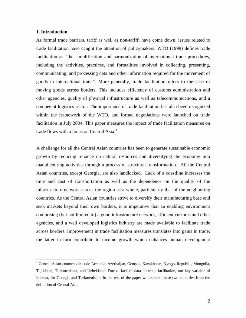
Since independence, the Central Asian economies have faced the challenge how to
generate sustained economic growth through a process of structural transformation and
reduced reliance on natural resources. As shown in Figure 1, exports of natural resources
constitute the bulk of total trade in the case of some the Central Asian countries. As much
as three-fourths of Azerbaijan’s exports and two-thirds of Kazakhstan’s are accounted for
by natural resources.2 The process of structural transformation involves a change in what
a country produces and a shift away from low-productivity, low-wage activities to high-
productivity and high-wage activities. A very clear example of structural transformation
is found in Asian economies such as the PRC, Vietnam, Malaysia, or the NIEs. The
output and employment structures are changing very fast in the direction of high value-
added sectors.
While the resource-rich Central Asian countries will continue to rely on natural resources
as the driver of economic growth, this has long term implications. First, is the well known
problem of the so-called Dutch disease. This refers to the negative effect that natural
resources tend to have on a country’s growth prospects. Resource exports cause the
country’s currency to appreciate making manufacturing activities uncompetitive. These
latter export activities might have had the potential to induce structural change. Second,
reliance on natural resources exposes the country to the vagaries of international markets.
Third, abundance in natural resources poses the problem of resource management and
rent seeking.
Fourth, and most relevant from the point of view of this paper, is that resource-rich
countries make for “bad neighbors” because of limited spillovers to surrounding
countries. This is important from the perspective of promoting greater regional
integration among the Central Asian countries. Enhancing intra-regional trade may offer
better potential for export upgrading than extra-regional trade. Increasing trade within the
same geographical region can be more conducive to diversification, structural change and
2 Natural resource exports covers SITC Rev 2 categories 0, 2, 3 and 4 which are food and live animals
chiefly for food, crude materials (inedible) except fuels, mineral fuels and related materials, and animal and
vegetable oils, fats and waxes, respectively.
4

industrial upgrading than trade with countries outside the region. It is not only the relative
pace of trade expansion but also the composition of intra-regional exports that makes
regional integration a promising strategy for accelerating economic development. Recent
literature (e.g., Hausmann et. al, 2007) has shown that the composition of exports impacts
long-term growth. In other words, countries with a more sophisticated export basket tend
to grow faster. Such a strategy relying on regional integration will require regional
production networks, a spatially coordinated expansion of regional infrastructure, and
better trade facilitation to encourage greater and timely flows of goods across borders.
Table 1 examines the extent of regional integration, as measured by intra-regional trade,
among the Central Asian countries. Intra-regional trade in Central Asia is lower than
within other regional arrangements such as the EU or ASEAN. Intra-regional trade in
manufacturing products accounted for only 1.6% of the total trade of Central Asian
countries in 2005, as opposed to 68% and 25% in case of the EU and ASEAN,
respectively.
Figure 2 shows the average un-weighted tariff rates for different groups of countries
categorized by income, and for a sub-group of the Central Asian countries (namely, the
CAREC countries).3 In all countries, including those in the CAREC region, tariffs have
fallen rapidly over the last decade. Tariffs in the CAREC countries are just above those of
the high income countries and far below those of the middle income and low income
countries. While tariffs are not prohibitively high in the CAREC countries, all of them are
landlocked which substantially increases trading cost and time as well as reliance on
infrastructure beyond one’s own borders (all countries in Central Asia are landlocked
except Georgia).
However, the Central Asian countries perform poorly when it comes to man-made non-
tariff barriers. These barriers take the form of inefficient customs administration and
other border agencies, long-delays at the ports, transit fees, unofficial payments, poor
3 CAREC countries include Azerbaijan, Kazakhstan, Kyrgyz Republic, Mongolia, Tajikistan, and
Uzbekistan.
5

physical infrastructure, and absence of a competent logistics sector. Man-made non tariff
barriers, such as those listed above, pose significant obstacles to trade. For example,
using the World Bank’s Doing Business Survey (World Bank, 2007b), the cost of
exporting (importing) a 20-foot container from/to is among the highest for the Central
Asian countries, not only in absolute US$ terms (see Figure 3).
Figure 4 provides a comparison of trade facilitation (measured by the LPI) in the Central
Asian countries with other countries. Not only are the Central Asian countries ranked the
lowest in terms of the overall index but are also at the bottom of the list when we
compare different components of LPI (see Figure 5). Clearly, there is scope for
improving trade facilitation in the region.
3. Literature Review
Gravity models are a widely used empirical approach to model bilateral trade flows. The
first empirical attempt to explain trade flows by the market size of the trading partners
and the distance between them goes back to Tinbergen (1962) and Pöyhönen (1963).4
The standard specification of the gravity model estimation involves GDP per capita (to
account for intra-industry trade and level of income), a measure of remoteness (this
captures the idea that it is the relative cost of trading that matters), adjacency and
geographical characteristics such as being landlocked. In this paper, we add a variable to
examine the impact of trade facilitation on bilateral trade flows. Recent developments in
the literature focus on choosing the right estimation procedure. We discuss some of the
estimation issues and the new developments in the next section.5
4 Anderson (1979) and Anderson and van Wincoop (2003) provide theoretical foundations for the gravity
model confirming its usefulness in empirical testing of bilateral trade flows. 5 An alternative to using the gravity model approach is to use CGE models to estimate the gains in trade
from improved trade facilitation. CGE models involve modeling trade facilitation as a reduction in the costs
of international trade or an improvement in the productivity of the international transportation sector
(Wilson et al., 2003).
6
Using a gravity model approach, Wilson et al. (2003) find that enhancing facilitation in
the APEC member countries will increase intra-APEC trade by as much as $254 billion
or a 21% increase. In a follow up paper (Wilson et al., 2005), using global bilateral trade
data, the authors show that improving the different components of trade facilitation
increases trade flows by $377 billion.
Djankov et al. (2006) use data on time taken to export and import from the World Bank’s
Doing Business Survey to estimate the impact of delays on trade. They show that each
additional day taken to move the goods from the firm’s warehouse to the ship reduces
trade by at least 1%. This is equivalent to a country distancing itself from its trade partner
by 85 km.
Limão and Venables (2001) show that deterioration in the infrastructure from the median
to the 75th percentile reduces trade volumes by 28%, which is equivalent to being 1,627
km away from trading partners. Fink et al. (2005) show that international variations in
bilateral communications costs have a significant influence on bilateral trade flows.
Hertel and Mirza (2009) show that trade facilitation reforms in South Asia translate into a
75% increase in intra-regional trade and a 22% increase in trade with the other regions.
In general, past studies on trade facilitation, using different measures of trade facilitation,
either incorporating all the possible dimensions of trade facilitation or by focusing on the
specific components, show that there are gains in trade from improving trade facilitation.
Wilson et al. (2003, 2005) include different measures from a variety of sources to include
the different components of trade facilitation. Djankov et al. (2006) use time taken to
export and import, from the World Bank’s Doing Business Survey, to measure the ease of
moving goods from firm’s warehouse to the ship. Other studies quoted above use
different components of trade facilitation. Hertel and Mirza (2009), on the other hand, use
the World Bank’s LPI (World Bank, 2007a) to capture trade facilitation. LPI and its sub-
components provide the first cross-country assessment of the logistics gap. It provides a
comprehensive picture of the different aspects of trade facilitation, ranging from customs
7
procedures to logistics costs, infrastructure quality to quality and competence of the
domestic logistics industry.
This paper also uses the same measure, LPI, to examine the impact of trade facilitation
and estimates the potential gains in trade from enhancing trade facilitation. There are,
however, important differences between this study and that of Hertel and Mirza (2009).
First, we tackle directly the problems arising from zero trade observations by using a
sample selection estimation procedure. Hertel and Mirza (2009) do not include zero trade
observations in their sample.6 This might result in biased estimates arising from sample
selection, an issue which we discuss in the next section. Second, while looking at the
different components of LPI we incorporate the different components of LPI in the same
equation whereas Hertel and Mirza (2009) estimate a different equation for each
component. This allows us to compare the effectiveness of the different components of
LPI directly. Third, we use 2005 data (Hertel and Mirza’s (2009) use 2001 data ) for 140
countries (Hertel and Mirza (2009) use a sample of 95 countries).
4. Estimation Strategy
The gravity model that we estimate is as follows:
0 1 2 3 4 5 6
7 8 9 10 11 12
ln( ) ln( ) ln( ) ln( ) ln( ) ln( ) ln
ln ln lnij ij i j i j i
j i j ij i j ij
T d GDP GDP GDPpc GDPpc LPI
LPI Landlocked Landlocked Border remote remote
β β β β β β β
β β β β β β
= + + + + + +
+ + + + + + ε+
(1)
where i denotes the exporter and j denotes the importer. The variables are defined as
follows. The dependent variable, Tij, is the bilateral trade flow in manufacturing products
from country i to country j.7 Dij is the distance between countries i and j. Size is captured
6 Their sample comprises of 95 countries which translates into 8,930 bilateral trading pairs. The number of
observations they report is only 3,614. 7 We also estimate the model using total trade and find that our results are qualitatively similar. However,
we restrict ourselves only to the bilateral trade in manufacturing products. This is because trade facilitation
measures for enhancing trade in natural resources are unlikely to be the same as for manufacturing goods.
For example, a gas pipeline will be exclusively used for exporting gas whereas improvements in domestic
logistics will help the manufacturing sector at large.
8

by the gross domestic product of the exporting (and the importing) country, GDPi
(GDPj). GDPpci (GDPpcj) is the GDP per capita of the exporting (and the importing
country). LPIi (LPIj) is the logistics performance index of the exporter (and the importer).
We are most interested in the coefficients of LPI, our measure of trade facilitation.
Landlocked is a dummy variable which takes on the value 1 if either the exporting (i) or
the importing (j) country is landlocked, and 0 otherwise. Border is also a dummy variable
takes on the value 0 if the trading partners share a common border, and 0 otherwise.8.
An important contribution of the Anderson and van Wincoop (2003) paper is that it
highlights that bilateral trade is determined by relative trading costs. In other words, it is
not just the distance between the two countries that matters; but also the bilateral distance
relative to the distance of the pair from their other trading partners. For example, consider
two trading pairs, Australia-New Zealand and Portugal-Slovakia. The distance between
the trading partners in the two pairs is similar. However, both Portugal and Slovakia have
other trading partners close by, whereas Australia and New Zealand do not. In other
words, Australia and New Zealand have fewer alternatives and therefore are likely to
trade more with each other. One way to control for the relative trading cost or the
multilateral resistance term is to use importer and exporter fixed effects. The main focus
of this paper is to study the impact of trade facilitation, which is measured at the country
level. Using importer and exporter fixed effect will wipe out the effect of trade
facilitation due to perfect multicollinearity. Instead, we control for remoteness using the
remotei (remotej) variable for the exporting country (and the importing country). It is
defined as the GDP-weighted average distance to all other countries (Figure 6 compares
the remoteness of select group of countries). Except for the indicator variables, all the
other variables used are in log terms.
A key estimation issue in gravity models is that of issue of zero bilateral trade.
Approximately 30% of the observations in our sample are zeros. This is important both
8 We do not consider the issue of “closed borders” or the “quality of the border”, i.e., countries that share a
border but, due to disputes, the border might be closed for trading purposes or countries might share a
border but may be unusable due to geographic terrain.
9

theoretically and econometrically. Theoretically, zero trade might not be missing
information and zero-trade may actually be reflecting the absence of any trade between
country pairs. If the zero trade data were randomly distributed, there would be little need
to worry about the issue. Figure 7 shows the distribution of zero trade across four
different sub-regions of the world. Clearly, the zeros are not randomly distributed, which
leads to the problem of selection bias if zero trade observations were to be dropped. In
other words, one needs to correct for the sample selection problem as zero trade might be
conveying important information. Recent papers such as Helpman et al. (2008) provide
theoretical underpinnings for zero trade. These papers argue that zero trade arises because
of the presence of fixed costs associated with establishing trade flows.
Econometrically, it is well known that zero values of the dependent variable can create
large biases (Tobin, 1958) and therefore, the choice of the estimation procedure becomes
important. Past studies using the gravity models suggest different ways of treating zero
trade observations. Common approaches include simply discarding them from the sample
(truncation), or adding a constant factor to each bilateral trade flow data so that zero trade
data does not drop out of the sample when working with logarithms. However, when
moving from a truncated sample to a sample containing zero values it is important to
change the estimation procedure and acknowledge the presence of zeros in the sample.
Not doing so will result in estimates being biased downwards. One such estimation
procedure is the Tobit technique. Limão and Venables (2001) used a Tobit estimator to
take into account the censored nature of the data. They replaced the zero trade
observations with the minimum value of trade flows in the sample.
More recently, Santos Silva and Tenreyro (2006) show that a log linear model estimated
by OLS leads to biased estimates in the presence of a heteroscedastic error term (a
consequence of Jensen’s inequality). They recommend using a Poisson Pseudo Maximum
Likelihood (PPML) estimator. Martin and Pham (2008) argue that while the PPML
estimator solves the problem of heteroscedasticity, it yields biased estimates when zero
trade values are frequent. Martin and Pham argue that standard threshold-Tobit estimators
perform better as long as the heteroscedastic nature of the error term is taken into account
10
adequately. They show that Heckman Maximum Likelihood estimators also perform well
if true identifying restrictions are available.
In this paper, we use the Heckman Maximum Likelihood estimator and use common
language, colonial ties and common colonizer as the exclusion restrictions. Common
language captures the cost related to cultural and linguistic barriers between two
countries. A firm exporting to a foreign country with connections from the past is likely
to be able to face lower fixed costs of entry into that country, as it does not incur large
adjustment costs arising from the unfamiliarity and the insecurity related to transaction
contingencies. All the three are indicator variables. Common language takes the value 1
if importer and exporter share a common language and zero otherwise. If importer (or
exporter) colonized its trading partner, then colonial ties takes the value 1 and 0
otherwise, and if both importer and exporter shared a common colonizer then common
colonizer takes the value 1 and 0 if not.
5. Data Sources
Data used in this paper comes from a variety of sources. The key data on bilateral trade
flows comes from Gaulier et. al (2008) for the year 2005.9 BACI data contains bilateral
trade flow data for almost 5,000 products (6-digit Harmonized System) and 200
countries. BACI data is based on the COMTRADE database. Each bilateral trade flow is
a weighted average of the exports and the corresponding mirror flow (adjusted for CIF).
Estimated qualities of reporting data are used as weights in the averaging of exports and
the corresponding mirror flows. Our key results are based on bilateral trade flows of
manufacturing goods corresponding to SITC Rev 2 categories 5 to 8 except 68.10 Given
the data availability for other countries, especially the LPI, we are left with 140 countries.
This results in 19,460 observations. According to the documentation accompanying the
9 Dataset is referred to as BACI in the paper. 10 Concordance from, with modifications, CEPII (Centre d'Etudes Prospectives et d'Informations
Internationales) and Jon Haveman
(http://www.macalester.edu/research/economics/page/haveman/Trade.Resources/tradeconcordances.html)
is used to map HS-6 to SITC Rev 2 (4-digit)
11
BACI dataset, data does not include flows below US$ 1,000. Consequently, after
aggregating manufacturing trade flows, any trade flow less than US$ 1,000 is treated as
zero trade.
We use GDP and GDP per capita for the year 2004 (to address any reverse causality
concerns) and both are measured in PPP terms. They are taken from the World
Development Indicators. Remoteness is calculated as the GDP-weighted average distance
to all other countries. Landlocked, common border, common language, colonial ties and
colonizer come from CEPII.
The key variable of interest in this paper is the measure of trade facilitation. We use the
World Bank’s Logistic Performance Index (World Bank, 2007a). We use the overall LPI
as well as examine the impact of its components separately. LPI is a composite measure
comprised of 7 variables: efficiency of customs and other border agencies, quality of
transport and information technology (IT) infrastructure, ease and affordability of
international shipments, competence of local logistics industry, ability to track and trace,
domestic logistics costs (this component is not used in the overall LPI as reported), and
timeliness of shipments in reaching destination. LPI is provided on a 5-point scale.
As shown in Table 2, these variables are highly correlated and any specification which
includes all six (domestic logistics is not used) will suffer from multicollinearity
problems. This will result in some of the components being statistically insignificant or
having a perverse sign. To avoid this problem we aggregate the components into 3
categories: customs efficiency, infrastructure, and logistics. Customs efficiency and
infrastructure correspond to efficiency of customs and other border agencies, and quality
of transport and IT infrastructure respectively. Logistics is a simple average of ease and
affordability of international shipments, competence of local logistics industry, and the
ability to track and trace.
Table 3 presents the summary statistics. The average trade flow within Central Asia is
almost 36 times smaller than that of the whole world. Countries in Central Asia region
12
are well below the world average for the LPI and its components (see Figures 4 and 5). In
our sample of 140 countries, there are 28 landlocked countries of which 7 are in Central
Asia.11
6. Results
6.1 Estimation Results
Table 4 shows the results from the estimation of equation 1. Estimates from the Heckman
ML estimation, our preferred estimator, are presented in Column 4. The first two columns
of Table 4 show the OLS estimates of equation 1 on the truncated sample, and the
censored OLS model in logarithms (with 1 added to all values of the dependent variable
to avoid the log-of-zero problem). Column 3 presents the results from Tobit estimation,
which replaces zero trade values in the sample with the minimum of the sample.
Comparing the coefficients in Columns 1 and 2 with those in Column 3 confirms that in
the case of a sample containing zero trade values, standard estimation procedures are
likely to bias downwards the estimated coefficients.
Column 4 presents the main results of the paper and the beta coefficients (to allow for
direct comparison of the importance of different variables) are shown in Table 5. Our
results are in line with the results found previously in the literature. Specifically, decrease
in distance by 1% increases trade by 1.56%. Size of the trading partners positively
impacts trade flows. While GDP per capita of the exporter has a positive and a
statistically significant impact on trade flows, GDP per capita of the importer does not
have any impact. Landlocked exporters (importers) trade 25% (38%) less than coastal
exporters (importers). Countries with a common border trade 2.4 times more than
countries that do not share a common border. In other words, having a common border is
11 Our sample has 19,460 bilateral trade observations. Of these, 432 have a common border with each other,
1,590 share a common language, 266 had a trading partner which colonized the other trading partner, and
1,546 share a common colonizer. Out of 42 trading relationships in Central Asia, 12 have a common
border, 2 share a common language, none had colonial ties with their partners, but 30 of them (all the
trading pairs excluding Mongolia) shared a common colonizer (note that the definition of colonizer here is
as defined in CEPII).
13

equivalent to a reduction in distance of about 3,147 km (evaluated at the mean distance).
Remoteness of the exporter has a positive and a statistically significant impact on trade
flows. Other things equal, if country A is farther from the rest of the world than country
B by 1%, then A’s exports to (imports from) a common third country C will be higher
than those of B by 0.43% (1.13%).
Our key variable of interest is LPI. We find that an improvement in trade facilitation
(LPI) of the exporting country by 1% increases exports by 5.5%. Trade facilitation of the
exporter has a higher impact on trade flows. An improvement in trade facilitation (LPI)
of the importing country by 1% boosts imports by 2.8%. 12
Column 5 shows the results using total trade as the dependent variable rather than trade in
manufacturing goods. Results using total trade as the dependent variable are qualitatively
similar to the ones obtained using trade in manufacturing goods only. The difference lies
in the magnitude of the coefficients of our variables of interest, namely the LPI of the
exporter and the importer. While LPI for the exporter is lower for total trade, LPI for the
importer is higher. There is no a priori reason to expect why the LPI of the exporter
should matter any less or why the LPI of the importer should matter more in the case of
total trade when compared with trade in manufacturing products. Since the difference
between the two columns is the trade in primary commodities, clearly that seems to be
the driving force. As discussed above, trade facilitation measures in the case of primary
commodities are likely to be different from those required for manufacturing products
which may be causing the difference in the estimated coefficients. We try to uncover
these differences across sectors in section 6.3 where we examine the role of trade
facilitation across different sectors.
12 We also estimate a specification with an additional variable, log of tariffs (results not shown). The data
on MFN tariffs is taken from CEPII’s MacMap database. Tariffs at the product level are averaged using the
corresponding share in total imports by country A from country B. We lose significant number of
observations due to lack of data on tariffs as well as lose the “square matrix” nature of our sample. We no
longer have 139 trading partners for each country. However, our results continue to hold qualitatively even
in the reduced sample.
14

We also examine the impact of the individual components of LPI. As discussed in section
5 due to potential multicollinearity, we use three categories of LPI—customs,
infrastructure, and logistics. Estimation results are presented in Table 6. The first column
reports the estimated coefficients, and the second shows the beta coefficients.
Coefficients on other variables are qualitatively similar to the benchmark result reported
in Table 4.
As expected, customs efficiency of the exporter has no impact on trade flows. It is the
customs efficiency of the importer, where all the documentation takes places, that
matters. Our results show that an improvement in customs efficiency of the importing
country by 1% improves trade flows by 1.04%. On the exporter side, it is infrastructure
that seems to have the greatest impact on trade flows, followed by the logistics of the
exporting country. On the other hand, for the importing country it is customs that matter
the most. Infrastructure and logistics of the importing country have a positive and a
statistically significant impact on trade flows but the impact is smaller than that derived
from improvement in customs efficiency.
Estimation results discussed above suggest that trade facilitation plays a very significant
role in enhancing trade flows. Further, different aspects of trade facilitation impact trade
differently. In the next section, we quantify the gains in trade from improvements in trade
facilitation.
6.2 “What-if” exercise
To quantify the effects of improvements in trade facilitation we do a simple “what-if”
exercise. The design of the exercise follows Wilson et al. (2003). The gravity model
results discussed above show that trade facilitation has a statistically significant trade-
enhancing effect. In this section we show that the gains are economically significant as
well. We quantify the potential increase in trade (both total trade and intra-regional trade)
derived from improving the overall LPI as well as the different components of LPI. This
15

will shed light on differences in benefits from various aspects of trade facilitation and
inform policymakers about gains from different kinds of trade facilitation measures.
Figures 4 and 5 show that trade facilitation in Central Asia, as measured by the LPI, is
among the poorest in the world and far below the average (Table 3). Some of the trade
facilitation measures, especially those related to infrastructure, are costly and time
consuming to implement. As a result, improvement in trade facilitation and its various
components in the Central Asian countries may happen in a phased manner rather than as
a one-off improvement in trade facilitation. As argued by Wilson et al. (2003), any
quantification of the gains in trade from enhancing trade facilitation measures must take
into account the feasibility of the improvements. Taking into account the feasibility
aspect, the exercise estimates the effect on total trade of improvement in the LPI of all the
nine Central Asian countries (as exporters and importers) up to halfway of the distance
between each country’s LPI and the average of all countries in the sample. Consequently,
the extent of the improvement in LPI differs across the different countries. For example,
Tajikistan, which has the lowest LPI, sees the highest improvement. Kyrgyz Republic,
which has the highest LPI among the Central Asian countries, has the smallest increase in
LPI.
Another feature of the exercise is that the estimated gains in trade are calculated taking
into account improvements in a country’s LPI as an exporter, and also considering the
improvement in its trading partners’ index. Note that the gravity equation contains the
LPI of both the exporter and the importer. For example, Azerbaijan’s exports increase as
a result of improving its trade facilitation but also as a result of the improvement in its
trading partners trade facilitation (i.e., those importing from Azerbaijan) in Central
Asia.13
Table 7 shows the gains in total trade with the rest of the world (exports plus imports)
from improvement in the overall LPI are significant. Overall trade of the Central Asian
13 Azerbaijan benefits from improvements in LPI of its trading partners in the Central Asia only because
LPI is assumed to change only for countries in the Central Asia.
16

countries increases by 44%. Tajikistan’s total trade increases by as much as 63%,
followed by Mongolia, 51%, Armenia, 49%, Kazakhstan and Uzbekistan, 47%, Kyrgyz
Republic, 34%, and Azerbaijan’s total trade increases by 28%. Increase in total trade due
to increase in imports is higher, as shown in Columns 2 and 3 of Table 7. This is because
imports are a greater share in total trade than exports. Column 1 of Table 5 shows that the
exporter’s estimated coefficient on LPI is higher than that for the importer. This is
reflected in the change in exports and imports seen separately (Table 8) and as expected
exports increase more than imports. Central Asia’s exports increase by 74% and imports
by 36%.
We also calculate the gains in intra-regional trade and find that intra-Central Asian trade (
from improvements in LPI) increases by as much as 100% (by construction, both intra-
Central Asian exports and imports increase by 100%). Change in intra-Central Asian
trade for the nine countries is shown in Table 9 (Table 10 shows the changes in exports
and imports).
Use of LPI as a measure of trade facilitation allows us to look at the different aspects of
the trade facilitation agenda such as customs efficiency, infrastructure and logistics.
Table 6 shows the estimated coefficients for the different components using the gravity
model. We estimate the gains in trade by repeating the same “what-if” exercise discussed
above, except that this time each of the three components, in the case of the Central Asian
countries, are improved to halfway of the sample average for the respective component.
Table 11 shows the gains in trade. The largest gains in total trade come from
improvement in infrastructure, followed by logistics and then improvement in the
customs efficiency of customs and other border agencies. However, one has to keep in
mind the cost aspect, time taken to complete, and ease of implementation. Regional
infrastructure will bring the maximum gains but the time taken to complete infrastructure
projects, costs involved and political economy issues of cross-border infrastructure
projects need to be weighed in. On other hand, improving customs efficiency, though it
results in smaller gains, may be easier to achieve as it relies largely on domestic reforms
and are less costly to implement.
17
6.3 Results by sector
The results so far discuss the gains in manufacturing sector trade from improving trade
facilitation. However, the importance of trade facilitation might differ across different
sectors within manufacturing. Table 12 shows the results of the gravity model estimated
for different sectors within the manufacturing sector. Here we discuss only the
coefficients on the trade facilitation measures, for all other variables results are similar as
in the benchmark regression. Column 1 of Table 12 reproduces the benchmark results in
Column 4 of Table 4. Column 2 shows the estimates using primary commodity exports.14
The LPI of the exporting country in the case of primary commodity exports has less
impact on trade flows than in the case of trade in manufacturing goods. This is also
reflected in the lower coefficient on LPI for exporter when using total trade in Column 5
of Table 4. This could be due to different trade facilitation requirements in the case of
primary exports.
Within the manufacturing sector (columns 3 to 8, Table 12) we find that LPI of the
exporting country for textiles & garments (column 3) and metals (column 4) has a similar
or a lower impact on bilateral trade flows than for total manufacturing trade. In the rest of
the sectors, with the exception of chemicals (column 5), LPI of the exporting country has
a greater impact on trade flows than for total manufacturing trade. In all sectors, the
impact of LPI of the importing country is similar to that for overall manufacturing. This
highlights that the trade facilitation measures in the exporting country are more important
and this difference is greater in sectors such as machinery (column 6), transport (column
7), and medical apparatus and optical instruments etc (column 8).
14 Primary commodities correspond to SITC Rev 2 categories 0 to 4 and 68. These correspond to food and
live animals chiefly for food (SITC Rev 2 category 0), beverages and tobacco (SITC Rev 2 category 1)
crude materials (inedible) except fuels (SITC Rev 2 category 2), mineral fuels and related materials (SITC
Rev 2 category 3), animal and vegetable oils, fats and waxes (SITC Rev 2 category 4), and non-ferrous
metals (SITC Rev 2 category 68).
18
One common characteristic of manufacturing goods where LPI of the exporting country
matters more than the total manufacturing exports is that they are more sophisticated,
differentiated, and high technology goods. In Table 13, we present results for
manufacturing goods classified according to their sophistication level, use of high
technology, and degree of differentiation. Our main focus is on the LPI variables and
results on other variables are similar to those in the benchmark regression. In Columns 1
and 2 of Table 13, we classify products as being highly sophisticated if they are in the top
quartile of the sophistication distribution (this variable is denoted as PRODY) and less
sophisticated if they are in the first quartile.15 We find that trade facilitation in the case of
the exporting country has a greater influence in the case of high PRODY products
(Column 2) than in the case of low PRODY products (Column 1) and for total
manufacturing exports (benchmark regressions).16 Among the manufacturing sectors,
most of the goods under machinery, transport, medical apparatus and optical instruments
etc., and a few of the chemical sector fall into high PRODY category. On the other hand,
most of the goods in the textiles & garments, and metals sector fall into the low PRODY
category.
In Columns 3 and 4 products are classified as high-tech and low-tech. We find that the
LPI of the exporting country matters more in the case of the high-tech products.17 In the
case of the high PRODY products and high technology products, LPI of the importing
country has a smaller impact on trade flows than in the case of overall manufacturing
trade flows (see benchmark regression). On the other hand, in the case of the low
PRODY and the low technology products, we find the opposite to be true i.e., LPI of the
15 Sophistication of the product is computed as the weighted average of the GDP per capita of all countries
exporting that product, where the weight reflect the revealed comparative advantage of the respective
country in that product (see Hausmann et al. (2007) for further details). 16 If we also classify products as being more sophisticated if their PRODY is above median in the
distribution of PRODYs and less sophisticated if PRODY is below the median, our results continue to hold
qualitatively. 17 Classification of goods as high technology goods comes from OECD (2008). We assume the rest, i.e. the
non-high technology products, to be low technology products.
19

importing country matters more for bilateral trade. In fact, in the low technology and the
low PRODY products, LPI of the importing country matters more.
Finally, in columns 5 to 7 three groups of products are formed using the classification
developed by Rauch (1999).18 This classification uses all products and not just
manufacturing sector. This classification categorizes products as being homogeneous and
differentiated. The homogenous goods are in turn divided into two categories—goods
traded on organized exchanges (e.g., commodities traded on London metal exchange such
as lead, steel, copper, aluminum) and goods not traded on organized exchanges but still
have a reference price (e.g., some chemicals). Our results show that trade facilitation
measures of the exporting country matter more for differentiated goods (Column 5). In
the case of the homogeneous goods (both traded on commodity exchanges and those with
a reference price), LPI of the importing country matters more. This could be due to the
fact that for commodities with organized exchanges and reference prices, there is little
role of trade facilitation and hence less incentive to improve the trade facilitation
measures in the exporting country. In the case of the differentiated goods, on the other
hand, trade facilitation measures by the exporting country act as a differentiation
mechanism from other countries.
In general, our results in Tables 12 and 13 show that an improvement in exporting
country’s trade facilitation leads to a greater increase in bilateral trade in highly
sophisticated goods, high technology products and more differentiated commodities than
increase in trade in less sophisticated, low technology and homogeneous commodities.
7 Conclusions and policy implications 18 Rauch (1999) classification is available online at
http://www.macalester.edu/research/economics/PAGE/HAVEMAN/Trade.Resources/Data/Classification/ra
uch_classification_rev2.xlsx. Some products that did not match with our trade data were dropped. We use
the liberal classification which maximizes the products categorized as homogeneous. Results using Rauch’s
conservative classification are qualitatively similar. It is to be noted that categorization of products as
highly sophisticated and high technology is based on HS-6 classification, Rauch classification is based on
SITC Rev 2.
20

Using a standard gravity model of bilateral trade flows, augmented to include a measure
of trade facilitation, we show that trade facilitation has a positive and a statistically
significant impact on bilateral trade flows. We also look at the different components of
trade facilitation. Our results show that, on the exporter side, it is the infrastructure that
has the greatest impact on trade flows; and on the importer side, it is the customs
efficiency that has the greatest impact on trade flows.
Our focus throughout the paper has been on the gains in trade in the case of the Central
Asian countries. These countries are ranked the lowest in terms of trade facilitation on the
basis of the World Bank’s cross-country LPI. Overall trade in the Central Asian countries
increases by 44% from improvements in LPI and intra-Central Asia trade doubles. The
increase in exports is greater than imports. However, because the share of imports in total
trade is higher imports contribute a larger share of the increase in total trade. In terms of
the different components, infrastructure improvements lead to the largest gains in trade,
followed by logistics and then customs. However, the gains should be weighed against
the ease of implementing. For example, from a short term perspective, improvements in
customs efficiency are relatively easier and cheaper to implement as opposed to
infrastructure. Though improvements in customs efficiency may deliver quicker results,
infrastructure is very important from the perspective of Central Asian countries,
especially given their landlocked nature. In what is a corollary of our findings,
developing regional infrastructure will provide transport corridors for trade within and
outside the region, help reduce trading time, further integrate countries in the region as
well with the rest of the world.
Further, our results show that the gains in trade resulting from improvement in trade
facilitation differ within the manufacturing sector. Increase in bilateral trade, due to an
improvement in exporting country’s LPI, in highly sophisticated, more differentiated and
high technology products is more than the increase in trade in less sophisticated, less
differentiated and low technology products. This is particularly important for the Central
Asian countries as they try to reduce dependence on natural resources, diversify
manufacturing and move towards higher value added. This will require these countries to
21

have access to international markets and in doing so trade facilitation has an important
role to play.
22

Bibliography Anderson, J. & E. van Wincoop. 2003. "Gravity with Gravitas: A Solution to the Border Puzzle." American Economic Review 93(1): 170-192. Anderson, J. 1979. "A Theoretical Foundation for the Gravity Equation." American Economic Review 69(1): 106-16. Djankov S., C. Freund, and C. Pham. 2006. Trading on Time. World Bank Policy Research Working Paper 3909. The World Bank, Washington, DC. Fink, C., A. Mattoo, and I. C. Neagu. 2005. "Assessing the Impact of Communication Costs on International Trade." Journal of International Economics 67(2): 428-445. Gaulier, G. and S. Zignago. July 2008 (draft). BACI: A World Database of International Trade at the Product-level: The 1995-2004. Centre d'Etudes Prospectives et d'Informations Internationales (CEPII). Hausmann, R., J. Hwang, and D. Rodrik. 2007. “What You Export Matters.” Journal of Economic Growth 12(1): 1-25. Helpman, E., M. Melitz and Y. Rubinstein. 2008. "Estimating Trade Flows: Trading Partners and Trading Volumes." The Quarterly Journal of Economics 123(2): 441-487. Hertel T. and and T. Mirza. 2009. "The Role of Trade Facilitation in South Asian Economic Integration." Study on Intraregional Trade and Investment in South Asia. ADB, Mandaluyong City. Limão, Nuno and A. J. Venables. 2001. "Infrastructure, Geographical Disadvantage, Transport Costs, and Trade." The World Bank Economic Review 15(3):451–479. Martin, W. and Pham, C. S. 2008. "Estimating the Gravity Equation when Zero Trade Flows are Frequent." Unpublished. MPRA Paper No. 9453, posted 05. July 2008/14:50. http://mpra.ub.uni-muenchen.de/9453/. OECD.2008. “Increasing the Relevance of Trade Statistics: Trade by High-Tech Products.” STD/SES/WPTGS(2008)10, OECD, Paris. van der Ploeg, F. and A. Venables. 2009. “Economic Integration in Central Asia”. Unpublished mimeograph. Pöyhönen, P. 1963. "A Tentative Model for the Volume of Trade Between Countries." Weltwirtschaftliches Archiv 90(1): 93-99. Rauch, J. E. 1999. “Networks versus Markets in International Trade.” Journal of International Economics 48(1): 7-35.
23

Santos Silva, J. M. C. and S. Tenreyro. 2006. "The Log of Gravity," The Review of Economics and Statistics 88(4): 641-658. Tinbergen, J. 1962. Shaping the World Economy: Suggestions for an International Economic Policy. The Twentieth Century Fund, New York. Tobin, J. 1958. Estimation of Relationships for Limited Dependent Variables,” Econometrica 26:24-36 Wilson, J., C. Mann and T. Otsuki. 2003. Trade Facilitation and Economic Development. World Bank Policy Research Working Paper 2988, The World Bank, Washington, DC.
Wilson, J., C. Mann and T. Otsuki. 2005. Assessing the Potential Benefit of Trade Facilitation: A Global Perspective. World Bank Policy Research Working Paper 3224, The World Bank, Washington, DC.
World Trade Organization. 1998. Report by the Secretariat on the March 1998 WTO Trade Facilitation Symposium.
World Bank. 2007a. Connecting to Compete: Trade Logistics in the Global Economy: The Logistics Performance Index and Its Indicators. The World Bank, Washington, DC. __________. 2007b. Doing Business 2007. The World Bank, Washington, DC.
24

Figure 1: Share of natural resources in total trade
0
20
40
60
80
100
0
20
40
60
80
100
1994
1996
1998
2000
2002
2004
2006
1994
1996
1998
2000
2002
2004
2006
1994
1996
1998
2000
2002
2004
2006
1994
1996
1998
2000
2002
2004
2006
1994
1996
1998
2000
2002
2004
2006
1994
1996
1998
2000
2002
2004
2006
1994
1996
1998
2000
2002
2004
2006
Armenia Azerbaijan Kazakhstan Kyrgyz Rep
Mongolia Tajikistan Uzbekistan
natural resources others
Exp
ort S
hare
(%)
Graphs by country
Source: UN COMTRADE
25

Figure 2: Tariff in CAREC countries Source: van der Ploeg and Venables (2009)
26
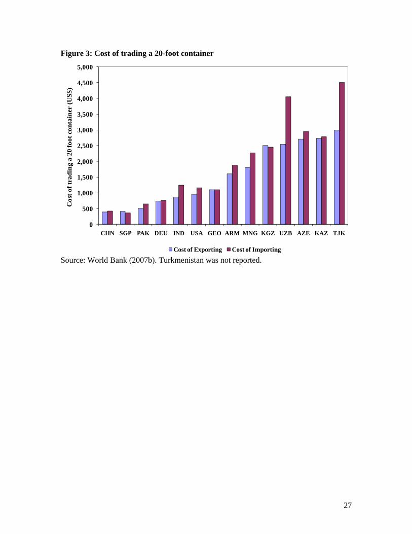
Figure 3: Cost of trading a 20-foot container
0
500
1,000
1,500
2,000
2,500
3,000
3,500
4,000
4,500
5,000
CHN SGP PAK DEU IND USA GEO ARM MNG KGZ UZB AZE KAZ TJK
Cos
t of t
radi
ng a
20
foot
con
tain
er (U
S$)
Cost of Exporting Cost of Importing Source: World Bank (2007b). Turkmenistan was not reported.
27
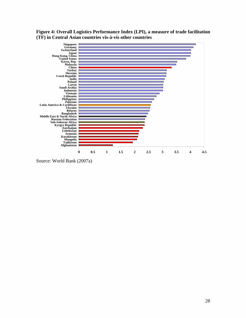
Figure 4: Overall Logistics Performance Index (LPI), a measure of trade facilitation (TF) in Central Asian countries vis-à-vis other countries
0 0.5 1 1.5 2 2.5 3 3.5 4 4.5
AfghanistanTajikistanMongolia
KazakhstanArmenia
UzbekistanAzerbaijan
Kyrgyz RepublicSub-Saharan AfricaRussian Federation
Middle East & North AfricaBangladesh
BelarusUkraine
Latin America & CaribbeanPakistan
PhilippinesLithuania
VietnamIndonesia
Saudi ArabiaLatviaPoland
IndiaCzech Republic
SloveniaTurkey
ChinaMalaysia
Korea, Rep.United States
Hong Kong, ChinaJapan
SwitzerlandGermany
Singapore
Source: World Bank (2007a)
28

Figure 5: Components of LPI
0
0.5
1
1.5
2
2.5
3
3.5
4
4.5
Overall LPI Customs Infrastructure Logistics Source: World Bank (2007), authors’ calculations
29

Figure 6: Remoteness
0 2000 4000 6000 8000 10000 12000 14000 16000
DNKNORSWEESTNLDFIN
LTUPOLSVKAUTCHEUKRGBRDEURUSESP
TURARMAZEKAZCANUZBKGZTJK
MNGPAKIND
KORGHACHNVNMUSAJPN
MEXTHAPHLSGPBRAIDNPRYARGCHLAUSNZL
Source: World Bank, CEPII, authors’ calculations
30

Figure 7: Zero trade by region
0%
10%
20%
30%
40%
50%
60%
70%
80%
90%
100%
Latin America
EU East Asia SAARC Central Asia Total
Positive trade in both directions Positive trade in one direction No trade in either direction Source: BACI, authors’ calculations
31

Table 1: Intra-regional trade in Central Asia vis-à-vis other regions
% of total trade which is
intra-regional % of trade in manufacturing goods which is intra-regional
Central Asia 4.8 1.6 ASEAN 27.4 25.3 SAARC 5.3 4.1 EU 63.7 68.3 Latin America 19.4 14.7 Source: BACI, authors’ calculations Table 2: Correlation between overall LPI and its components
Overall LPI Customs Infrastructure
Ease of arranging international shipments
Competence of local logistics
Ability to track and trace
Timeliness of shipments
Overall LPI 1 Customs 0.97 1 Infrastructure 0.97 0.96 1 Ease of arranging international shipments
0.96 0.91 0.91 1
Competence of local logistics
0.98 0.94 0.94 0.94 1
Ability to track and trace
0.97 0.93 0.93 0.91 0.94 1
Timeliness of shipments 0.93 0.88 0.87 0.86 0.88 0.89 1
Source: World Bank (2007a), authors’ calculations
32
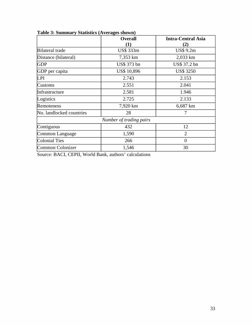
Table 3: Summary Statistics (Averages shown) Overall
(1) Intra-Central Asia
(2) Bilateral trade US$ 333m US$ 9.2m Distance (bilateral) 7,353 km 2,033 km GDP US$ 373 bn US$ 37.2 bn GDP per capita US$ 10,896 US$ 3250 LPI 2.743 2.153 Customs 2.551 2.041 Infrastructure 2.581 1.946 Logistics 2.725 2.133 Remoteness 7,920 km 6,687 km No. landlocked countries 28 7
Number of trading pairs Contiguous 432 12 Common Language 1,590 2 Colonial Ties 266 0 Common Colonizer 1,546 30 Source: BACI, CEPII, World Bank, authors’ calculations
33
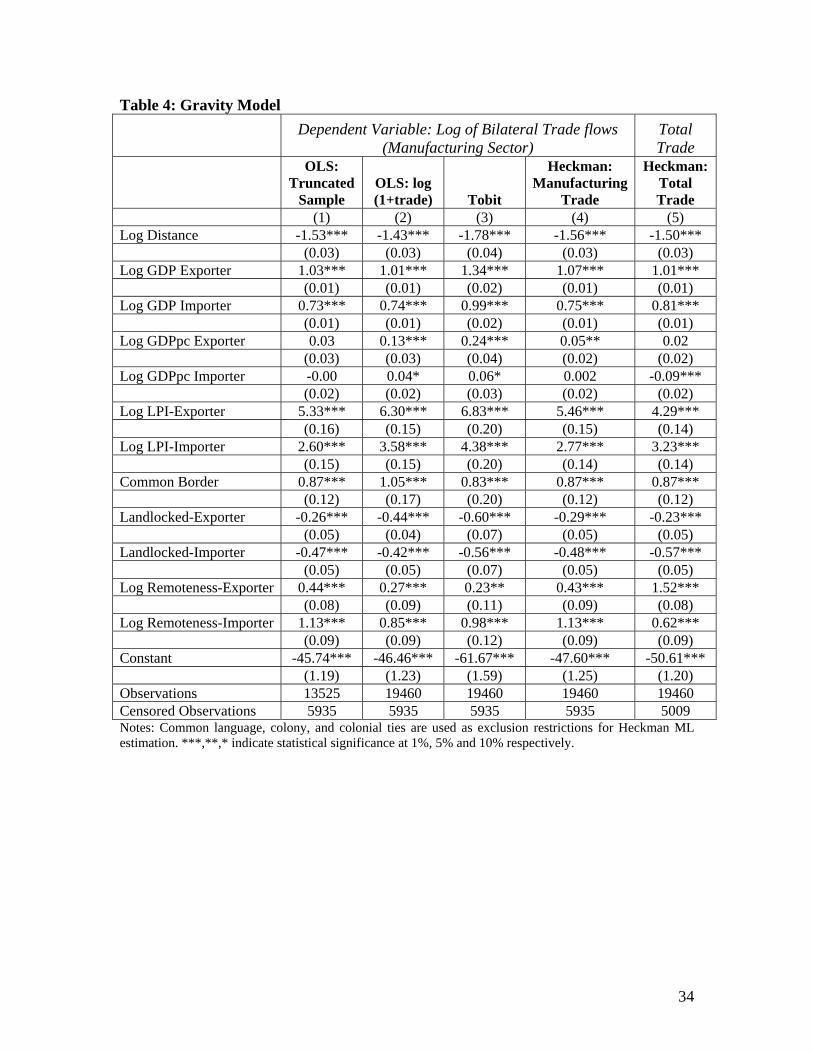
Table 4: Gravity Model
Dependent Variable: Log of Bilateral Trade flows
(Manufacturing Sector) Total Trade
OLS: Truncated
Sample OLS: log (1+trade) Tobit
Heckman: Manufacturing
Trade
Heckman: Total Trade
(1) (2) (3) (4) (5) Log Distance -1.53*** -1.43*** -1.78*** -1.56*** -1.50*** (0.03) (0.03) (0.04) (0.03) (0.03) Log GDP Exporter 1.03*** 1.01*** 1.34*** 1.07*** 1.01*** (0.01) (0.01) (0.02) (0.01) (0.01) Log GDP Importer 0.73*** 0.74*** 0.99*** 0.75*** 0.81*** (0.01) (0.01) (0.02) (0.01) (0.01) Log GDPpc Exporter 0.03 0.13*** 0.24*** 0.05** 0.02 (0.03) (0.03) (0.04) (0.02) (0.02) Log GDPpc Importer -0.00 0.04* 0.06* 0.002 -0.09*** (0.02) (0.02) (0.03) (0.02) (0.02) Log LPI-Exporter 5.33*** 6.30*** 6.83*** 5.46*** 4.29*** (0.16) (0.15) (0.20) (0.15) (0.14) Log LPI-Importer 2.60*** 3.58*** 4.38*** 2.77*** 3.23*** (0.15) (0.15) (0.20) (0.14) (0.14) Common Border 0.87*** 1.05*** 0.83*** 0.87*** 0.87*** (0.12) (0.17) (0.20) (0.12) (0.12) Landlocked-Exporter -0.26*** -0.44*** -0.60*** -0.29*** -0.23*** (0.05) (0.04) (0.07) (0.05) (0.05) Landlocked-Importer -0.47*** -0.42*** -0.56*** -0.48*** -0.57*** (0.05) (0.05) (0.07) (0.05) (0.05) Log Remoteness-Exporter 0.44*** 0.27*** 0.23** 0.43*** 1.52*** (0.08) (0.09) (0.11) (0.09) (0.08) Log Remoteness-Importer 1.13*** 0.85*** 0.98*** 1.13*** 0.62*** (0.09) (0.09) (0.12) (0.09) (0.09) Constant -45.74*** -46.46*** -61.67*** -47.60*** -50.61*** (1.19) (1.23) (1.59) (1.25) (1.20) Observations 13525 19460 19460 19460 19460 Censored Observations 5935 5935 5935 5935 5009 Notes: Common language, colony, and colonial ties are used as exclusion restrictions for Heckman ML estimation. ***,**,* indicate statistical significance at 1%, 5% and 10% respectively.
34

Table 5: Benchmark specification and beta coefficients Dependent Variable: Log of Bilateral Trade flows (Manufacturing Sector)
Estimated Coefficient (1)
Beta Coefficient (2)
Log Distance -1.56*** -0.25 Log GDP Exporter 1.07*** 0.45 Log GDP Importer 0.75*** 0.32 Log GDPpc Exporter 0.05** 0.01 Log GDPpc Importer 0.002 0.0004 Log LPI-Exporter 5.46*** 0.24 Log LPI-Importer 2.77*** 0.12 Common Border 0.87*** 0.03 Landlocked-Exporter -0.29*** -0.02 Landlocked-Importer -0.48*** -0.04 Log Remoteness-Exporter 0.43*** 0.02 Log Remoteness-Importer 1.13*** 0.05 Observations 19,460 Estimated coefficients are the ones reported in Column 4 of Table 3. ***,**,* indicates statistical significance at 1%, 5% and 10%
35

Table 6: Gravity Model using components of LPI and beta coefficients Dependent Variable: Log of Bilateral Trade Flows (Manufacturing Sector)
Estimated Coefficient
(1) Beta Coefficient
(2) Log Distance -1.55*** -0.25 (0.028) Log GDP Exporter 1.06*** 0.45 (0.013) Log GDP Importer 0.76*** 0.32 (0.013) Log GDPpc Exporter -0.02 -0.005 (0.03) Log GDPpc Importer -0.02 -0.005 (0.02) Log Customs- Exporter -0.001 -0.00003 (0.26) Log Customs- Importer 1.04*** 0.05 (0.26) Log Infrastructure- Exporter 3.09*** 0.16 (0.28) Log Infrastructure- Importer 0.86*** 0.04 (0.27) Log Logistics- Exporter 2.19*** 0.10 (0.26) Log Logistics- Importer 0.75*** 0.03 (0.25) Common Border 0.90*** 0.03 (0.12) Landlocked-Exporter -0.24*** -0.02 (0.05) Landlocked-Importer -0.45*** -0.04 (0.05) Log Remoteness-Exporter 0.36*** 0.02 (0.09) Log Remoteness-Importer 1.11*** 0.05 (0.09) Observations 19,460 Notes: Heckman ML estimation procedure is used (constant is included but not shown here). Common language, colony, and colonial ties are used as exclusion restrictions. ***,**,* indicate statistical significance at 1%, 5% and 10% respectively.
36

Table 7: Gains in total trade from improvement in overall LPI
% change in total trade Due to exports Due to imports
(1) (2) (3) Armenia 49.2 (15.3) 25.5 23.7 Azerbaijan 28.4 (9.6) 3.2 25.2 Kazakhstan 46.8 (14.3) 16.6 30.2 Kyrgyz Republic 34.1 (16.0) 12.3 21.8 Mongolia 50.8 (23.5) 18.6 32.2 Tajikistan 62.5 (15.7) 11.2 51.3 Uzbekistan 46.6 (11.7) 20.3 26.3 Numbers in brackets are percentage point increase in total trade as share of GDP in 2005 Table 8: Change in total exports and imports from improvement in overall LPI As Exporter As Importer % Change in total exports % Change in total imports Armenia 72 (7.9) 37 (7.4) Azerbaijan 54 (1.1) 27 (8.5) Kazakhstan 76 (5.1) 39 (9.2) Kyrgyz Republic 62 (5.8) 27 (10.2) Mongolia 81 (8.6) 42 (14.9) Tajikistan 105 (2.8) 57 (12.9) Uzbekistan 73 (5.1) 37 (6.6) Numbers in brackets are percentage point increase in exports or imports as share of GDP in 2005
37

Table 9: Gains in intra-Central Asia trade from improvement in overall LPI
% change in total trade Due to exports Due to imports
(1) (2) (3) Armenia 108.8 52.6 56.3 Azerbaijan 95.3 26.7 68.6 Kazakhstan 100.8 49.0 51.8 Kyrgyz Republic 88.0 51.7 36.3 Mongolia 115.2 4.0 111.2 Tajikistan 115.8 3.7 112.1 Uzbekistan 103.5 70.2 33.3 Table 10: Change in intra-Central Asia exports and imports from improvement in overall LPI As Exporter As Importer
% Change in exports to Central Asian countries
% Change in imports from Central Asian countries
Armenia 109 109 Azerbaijan 88 98 Kazakhstan 107 95 Kyrgyz Republic 84 95 Mongolia 111 115 Tajikistan 137 115 Uzbekistan 104 103
38

Table 11: Gains in total trade from improvement in different components of LPI % change in total trade
Infrastructure (1)
Customs (2)
Logistics (3)
Armenia 33.6 6.9 17.2 Azerbaijan 14.1 6.9 7.8 Kazakhstan 24.4 12.8 14.7 Kyrgyz Republic 19.7 7.8 10.4 Mongolia 22.4 10.4 15.3 Tajikistan 18.1 14.5 20.6 Uzbekistan 21.3 11.5 16.7 Each cell shows the percent increase in total trade (exports + imports) from improvement in different components of LPI
39

Table 12: Estimates of gravity model using sector level trade
All manufacturing goods
Primary products
Textiles & garments Metals Chemicals Machinery Transport Medical appartus &
optical instruments
(1) (2) (3) (4) (5) (6) (7) (8)Log Distance -1.56*** -1.39*** -1.59*** -1.81*** -1.72*** -1.53*** -1.65*** -1.17***
(0.03) (0.03) (0.04) (0.04) (0.03) (0.03) (0.04) (0.03)Log GDP Exporter 1.07*** 0.78*** 1.08*** 1.22*** 1.00*** 1.00*** 1.17*** 0.97***
(0.01) (0.02) (0.02) (0.02) (0.02) (0.02) (0.02) (0.02)Log GDP Importer 0.75*** 0.76*** 0.67*** 0.68*** 0.82*** 0.75*** 0.65*** 0.78***
(0.01) (0.01) (0.02) (0.02) (0.02) (0.02) (0.02) (0.02)Log GDPpc Exporter 0.05** -0.16*** -0.70*** -0.01 0.21*** -0.05 -0.20*** 0.02
(0.02) (0.03) (0.03) (0.03) (0.03) (0.03) (0.04) (0.03)Log GDPpc Importer 0.00 -0.13*** 0.22*** 0.10*** -0.03 0.13*** 0.08** 0.18***
(0.02) (0.03) (0.03) (0.03) (0.03) (0.03) (0.04) (0.03)Log LPI-Exporter 5.46*** 3.46*** 5.46*** 3.45*** 4.52*** 8.60*** 7.21*** 7.85***
(0.15) (0.17) (0.20) (0.19) (0.18) (0.18) (0.25) (0.20)Log LPI-Importer 2.77*** 2.54*** 2.64*** 1.84*** 1.28*** 2.05*** 2.26*** 2.29***
(0.14) (0.16) (0.19) (0.18) (0.17) (0.17) (0.22) (0.17)Commom Border 0.87*** 1.09*** 0.73*** 1.05*** 0.83*** 0.90*** 0.90*** 0.85***
(0.12) (0.12) (0.14) (0.13) (0.12) (0.13) (0.15) (0.12)Landlocked-Exporter -0.29*** -0.30*** -0.29*** 0.05 -0.33*** -0.03 0.21** 0.19***
(0.05) (0.06) (0.07) (0.07) (0.06) (0.06) (0.08) (0.07)Landlocked-Importer -0.48*** -0.66*** -0.43*** -0.68*** -0.43*** -0.20*** -0.56*** 0.02
(0.05) (0.05) (0.06) (0.06) (0.06) (0.06) (0.08) (0.06)Log Remoteness-Exporter 0.43*** 2.60*** 1.07*** 0.28*** 0.47*** 0.48*** 0.61*** 0.51***
(0.09) (0.10) (0.11) (0.11) (0.10) (0.10) (0.13) (0.10)Log Remoteness-Importer 1.13*** -0.12 0.90*** 1.64*** 2.14*** 1.25*** 0.97*** 0.99***
(0.09) (0.10) (0.11) (0.11) (0.10) (0.10) (0.14) (0.11)Constant -47.61*** -45.65*** -47.21*** -50.51*** -56.20*** -52.26*** -50.23*** -56.66***
(1.25) (1.37) (1.65) (1.61) (1.47) (1.45) (1.94) (1.51)Observations 19460 19460 19460 19460 19460 19460 19460 19460Censored Observations 5935 7329 9537 9856 9749 8471 11308 11405
Dependent variable: log of bilateral trade flows (overall or sectoral as specified)
Notes: Heckman ML estimation procedure is used (constant is included but not shown here). Common language, colony, and colonial ties are used as exclusion restrictions. ***,**,* indicate statistical significance at 1%, 5% and 10% respectively.
40
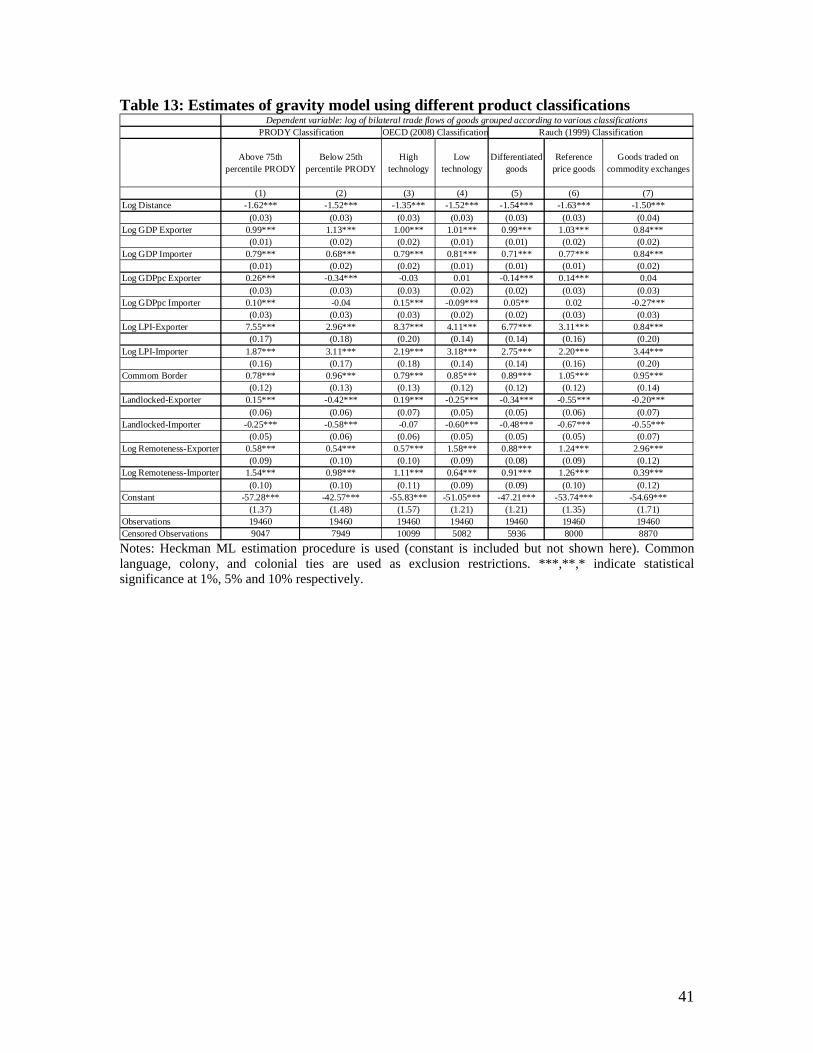
Table 13: Estimates of gravity model using different product classifications
Above 75th percentile PRODY
Below 25th percentile PRODY
High technology
Low technology
Differentiated goods
Reference price goods
Goods traded on commodity exchanges
(1) (2) (3) (4) (5) (6) (7)Log Distance -1.62*** -1.52*** -1.35*** -1.52*** -1.54*** -1.63*** -1.50***
(0.03) (0.03) (0.03) (0.03) (0.03) (0.03) (0.04)Log GDP Exporter 0.99*** 1.13*** 1.00*** 1.01*** 0.99*** 1.03*** 0.84***
(0.01) (0.02) (0.02) (0.01) (0.01) (0.02) (0.02)Log GDP Importer 0.79*** 0.68*** 0.79*** 0.81*** 0.71*** 0.77*** 0.84***
(0.01) (0.02) (0.02) (0.01) (0.01) (0.01) (0.02)Log GDPpc Exporter 0.26*** -0.34*** -0.03 0.01 -0.14*** 0.14*** 0.04
(0.03) (0.03) (0.03) (0.02) (0.02) (0.03) (0.03)Log GDPpc Importer 0.10*** -0.04 0.15*** -0.09*** 0.05** 0.02 -0.27***
(0.03) (0.03) (0.03) (0.02) (0.02) (0.03) (0.03)Log LPI-Exporter 7.55*** 2.96*** 8.37*** 4.11*** 6.77*** 3.11*** 0.84***
(0.17) (0.18) (0.20) (0.14) (0.14) (0.16) (0.20)Log LPI-Importer 1.87*** 3.11*** 2.19*** 3.18*** 2.75*** 2.20*** 3.44***
(0.16) (0.17) (0.18) (0.14) (0.14) (0.16) (0.20)Commom Border 0.78*** 0.96*** 0.79*** 0.85*** 0.89*** 1.05*** 0.95***
(0.12) (0.13) (0.13) (0.12) (0.12) (0.12) (0.14)Landlocked-Exporter 0.15*** -0.42*** 0.19*** -0.25*** -0.34*** -0.55*** -0.20***
(0.06) (0.06) (0.07) (0.05) (0.05) (0.06) (0.07)Landlocked-Importer -0.25*** -0.58*** -0.07 -0.60*** -0.48*** -0.67*** -0.55***
(0.05) (0.06) (0.06) (0.05) (0.05) (0.05) (0.07)Log Remoteness-Exporter 0.58*** 0.54*** 0.57*** 1.58*** 0.88*** 1.24*** 2.96***
(0.09) (0.10) (0.10) (0.09) (0.08) (0.09) (0.12)Log Remoteness-Importer 1.54*** 0.98*** 1.11*** 0.64*** 0.91*** 1.26*** 0.39***
(0.10) (0.10) (0.11) (0.09) (0.09) (0.10) (0.12)Constant -57.28*** -42.57*** -55.83*** -51.05*** -47.21*** -53.74*** -54.69***
(1.37) (1.48) (1.57) (1.21) (1.21) (1.35) (1.71)Observations 19460 19460 19460 19460 19460 19460 19460Censored Observations 9047 7949 10099 5082 5936 8000 8870
PRODY Classification OECD (2008) Classification Rauch (1999) ClassificationDependent variable: log of bilateral trade flows of goods grouped according to various classifications
Notes: Heckman ML estimation procedure is used (constant is included but not shown here). Common language, colony, and colonial ties are used as exclusion restrictions. ***,**,* indicate statistical significance at 1%, 5% and 10% respectively.
41

42
Appendix Table 2: Change in LPI Initial LPI New LPI % change in LPIArmenia 2.14 2.44 13.50% Azerbaijan 2.29 2.52 10.04% Kazakhstan 2.12 2.43 14.62% Kyrgyz Republic 2.35 2.55 8.51% Mongolia 2.08 2.41 15.86% Tajikistan 1.93 2.34 21.24% Uzbekistan 2.16 2.45 13.42%