The Role of Time-Varying Contextual Factors in Latent

Zurich Open Repository andArchiveUniversity of ZurichMain LibraryStrickhofstrasse 39CH-8057 Zurichwww.zora.uzh.ch

Year: 2021

The role of time-varying contextual factors in latent attrition models forcustomer base analysis

Bachmann, Patrick ; Meierer, Markus ; Näf, Jeffrey

Abstract: Customer base analysis of noncontractual businesses builds on modeling purchases and latentattrition. With the Pareto/NBD model, this has become a straightforward exercise. However, thissimplicity comes at a price. Customer-level predictions often lack precision. This issue can be addressedby acknowledging the importance of contextual factors for customer behavior. Considering contextualfactors might contribute in two ways: (1) by increasing predictive accuracy and (2) by identifying theimpact of these determinants on the purchase and attrition process. However, there is no generalizationof the Pareto/NBD model that incorporates time-varying contextual factors. Preserving a closed-formmaximum likelihood solution, this study proposes an extension that facilitates modeling time-invariantand time-varying contextual factors in continuous noncontractual settings. These contextual factors caninfluence the purchase process, the attrition process, or both. The authors further illustrate how tocontrol for endogenous contextual factors. Benchmarking with three data sets from the retailing industryshows that explicitly modeling time-varying contextual factors significantly improves the accuracy ofout-of-sample predictions for future purchases and latent attrition.

DOI: https://doi.org/10.1287/mksc.2020.1254

Posted at the Zurich Open Repository and Archive, University of ZurichZORA URL: https://doi.org/10.5167/uzh-197236Journal ArticlePublished Version

The following work is licensed under a Creative Commons: Attribution 4.0 International (CC BY 4.0)License.

Originally published at:Bachmann, Patrick; Meierer, Markus; Näf, Jeffrey (2021). The role of time-varying contextual factors inlatent attrition models for customer base analysis. Marketing Science, 40(4):783-809.DOI: https://doi.org/10.1287/mksc.2020.1254

This article was downloaded by: [130.60.36.151] On: 21 January 2021, At: 04:38Publisher: Institute for Operations Research and the Management Sciences (INFORMS)INFORMS is located in Maryland, USA

Marketing Science

Publication details, including instructions for authors and subscription information:http://pubsonline.informs.org

The Role of Time-Varying Contextual Factors in LatentAttrition Models for Customer Base AnalysisPatrick Bachmann, Markus Meierer, Jeffrey Näf

To cite this article:Patrick Bachmann, Markus Meierer, Jeffrey Näf (2021) The Role of Time-Varying Contextual Factors in Latent Attrition Modelsfor Customer Base Analysis. Marketing Science

Published online in Articles in Advance 15 Jan 2021

. https://doi.org/10.1287/mksc.2020.1254

Full terms and conditions of use: https://pubsonline.informs.org/Publications/Librarians-Portal/PubsOnLine-Terms-and-Conditions

This article may be used only for the purposes of research, teaching, and/or private study. Commercial useor systematic downloading (by robots or other automatic processes) is prohibited without explicit Publisherapproval, unless otherwise noted. For more information, contact [email protected].

The Publisher does not warrant or guarantee the article’s accuracy, completeness, merchantability, fitnessfor a particular purpose, or non-infringement. Descriptions of, or references to, products or publications, orinclusion of an advertisement in this article, neither constitutes nor implies a guarantee, endorsement, orsupport of claims made of that product, publication, or service.

Copyright © 2021, The Author(s)

Please scroll down for article—it is on subsequent pages

With 12,500 members from nearly 90 countries, INFORMS is the largest international association of operations research (O.R.)and analytics professionals and students. INFORMS provides unique networking and learning opportunities for individualprofessionals, and organizations of all types and sizes, to better understand and use O.R. and analytics tools and methods totransform strategic visions and achieve better outcomes.For more information on INFORMS, its publications, membership, or meetings visit http://www.informs.org

http://pubsonline.informs.org

https://doi.org/10.1287/mksc.2020.1254

https://pubsonline.informs.org/Publications/Librarians-Portal/PubsOnLine-Terms-and-Conditions

https://pubsonline.informs.org/Publications/Librarians-Portal/PubsOnLine-Terms-and-Conditions

http://www.informs.org

MARKETING SCIENCEArticles in Advance, pp. 1–38

http://pubsonline.informs.org/journal/mksc ISSN 0732-2399 (print), ISSN 1526-548X (online)

The Role of Time-Varying Contextual Factors in Latent AttritionModels for Customer Base Analysis

Patrick Bachmann,a Markus Meierer,a Jeffrey Näfb

aUniversity Research Priority Program Social Networks, University of Zurich, 8050 Zurich, Switzerland; bDepartment of Mathematics,Eidgenossische Technische Hochschule (ETH) Zurich, 8092 Zurich, Switzerland

Contact: [email protected], https://orcid.org/0000-0002-3938-2697 (PB); [email protected],https://orcid.org/0000-0003-1995-5897 (MM); [email protected], https://orcid.org/0000-0003-0920-1899 (JN)

Received: July 5, 2017

Revised: August 3, 2018; April 16, 2019;September 17, 2019; March 12, 2020

Accepted: May 12, 2020

Published Online in Articles in Advance:January 15, 2021


Copyright: © 2021 The Author(s)

Abstract. Customer base analysis of noncontractual businesses builds on modelingpurchases and latent attrition. With the Pareto/NBD model, this has become a straight-forward exercise. However, this simplicity comes at a price. Customer-level predictionsoften lack precision. This issue can be addressed by acknowledging the importance ofcontextual factors for customer behavior. Considering contextual factors might contributein twoways: (1) by increasing predictive accuracy and (2) by identifying the impact of thesedeterminants on the purchase and attrition process. However, there is no generalization ofthe Pareto/NBD model that incorporates time-varying contextual factors. Preserving aclosed-formmaximum likelihood solution, this study proposes an extension that facilitatesmodeling time-invariant and time-varying contextual factors in continuous noncontractualsettings. These contextual factors can influence the purchase process, the attrition process,or both. The authors further illustrate how to control for endogenous contextual factors.Benchmarking with three data sets from the retailing industry shows that explicitlymodeling time-varying contextual factors significantly improves the accuracy of out-of-sample predictions for future purchases and latent attrition.

History: Yuxin Chen served as the senior editor and Peter Fader served as associate editor for this article.Open Access Statement: This work is licensed under a Creative Commons Attribution- NonCommercial 4.0

International License. You are free to download this work and share with others for any purpose, exceptcommercially, and you must attribute this work as “Marketing Science. Copyright © 2020 The Author(s).https://doi.org/10.1287/mksc.2020.1254, used under a Creative Commons Attribution License: https://creativecommons.org/licenses/by-nc/4.0/.”

Funding: This work was funded by the University Research Priority Program Social Networks at theUniversity of Zurich and the Swiss National Science Foundation [Project 100018_163189].

Supplemental Material: The data files and online appendix are available at https://doi.org/10.1287/mksc.2020.1254.

Keywords: probability models • Pareto/NBD • customer relationship management • latent attrition • contextual factors • customer lifetime value

1. IntroductionModeling customer purchases and attrition in non-contractual businesses has become a straightforwardtask, but this simplicity comes at a price. Havingaccess to recency and frequency data of customers’past transactions allows marketers to apply the Pareto/NBD model (Schmittlein et al. 1987). However, pre-dictions are said to represent an educated guess ratherthan a precise value (Wübben andWangenheim 2008,Malthouse 2009, Fader 2012). If the focus is on theaggregated level, that is, the entire customer base, thisdifference can be rather negligible. In contrast, theapplicability of individual level predictions is oftenlimited. For example, an increased level of precision isrequired when allocating resources for customer re-tention activities to individual customers.

There have been many attempts to improve theoriginal Pareto/NBD model. However, there existsno generalization that allows modeling time-varying

contextual factors in a continuous noncontractualsetting. Extensions to the Pareto/NBD model or re-lated models mainly focus on the computationalcomplexity of the estimation procedure (Fader et al.2005a), the correlation between the modeled pro-cesses (Glady et al. 2015), or the integration of time-invariant contextual factors (Fader and Hardie 2007,Abe 2009, Singh et al. 2009). Recent studies illustratehow regularity patterns (Platzer and Reutterer 2016)and stationary transaction attributes can be includedin the customer’s purchase process (Braun et al. 2015)or how differences across customer cohorts may becaptured in latent attrition models (Gopalakrishnanet al. 2017). An approach by Schweidel and Knox(2013) goes one step further and provides the possi-bility of including other time-varying contextual fac-tors (i.e. direct mailing activity) into a discrete latentattrition model. Although the Pareto/NBD model isvery popular in research and practice, no extension

1

http://pubsonline.informs.org/journal/mksc

mailto:[email protected]

https://orcid.org/0000-0002-3938-2697

https://orcid.org/0000-0002-3938-2697


https://orcid.org/0000-0003-1995-5897

https://orcid.org/0000-0003-1995-5897


https://orcid.org/0000-0003-0920-1899

https://orcid.org/0000-0003-0920-1899



https://creativecommons.org/licenses/by-nc/4.0/

https://creativecommons.org/licenses/by-nc/4.0/



allows for the inclusion of time-varying contex-tual factors.

The impact of two broad categories of time-varyingcontextual factors on customer behavior has beenhighlighted in the previous literature (Schweidel andKnox 2013, Hanssens and Pauwels 2016): (1) sea-sonality in purchase patterns and (2) tactical mar-keting activities. Seasonality in purchase patternsis common in many noncontractual settings, espe-cially in the retailing industry. Customer behavior isheavily influenced at the aggregate level by publicholidays (e.g., Christmas and Thanksgiving) and atthe individual level by recurring personal events (e.g.,birthdays and paydays). In addition to seasonality,tactical marketing activities are an important time-varying determinant of customer behavior. Customerscan be targeted by either individual- or aggregate-leveltactical marketing activities, such as personalized ormass marketing campaigns. Explicitly modeling mar-keting variables, such as time-varying contextual factors,explains the heterogeneity across customers that wasintroduced by the firm in the first place. Including eitherkind of time-varying contextual factors improves thepredictive accuracy of probabilistic customer attritionmodels. However, the impact of these contextual factorsis likely to vary. Probabilistic customer attrition modelsoperationalize customer behavior through two pro-cesses: (1) the purchase process and (2) the attritionprocess. When contextual factors are added to themodel, they are allowed to influence customer be-havior through these two processes. However, thesefactors do not necessarily have to affect both pro-cesses. It is reasonable that some of the contextualfactors influence only customers’ purchases or attri-tion. For example, although personalized couponingwill likely impact only the purchase process, directmailing information about loyaltyprogrameventsmightonly impact the attrition process. Furthermore, it is avalid assumption that marketing activities irritate cus-tomers and thus increase customer attrition (Ascarzaet al. 2016). Similarly, seasonality patterns, such asthose caused by holiday seasons, are likely to have anexclusive impact on the purchase process, whereasother seasonality patterns, such as those caused byindividual paydays might additionally impact cus-tomer attrition. The latter may cause customers to re-consider their existing business relationships. Being ableto test such hypotheses is a desired feature when ana-lyzing contextual factors in latent attrition models.

In this paper, we propose a latent attrition modelthat allows time-varying contextual factors to bemodeled in continuous noncontractual settings. Com-plementing previous literature, we combine the fol-lowing characteristics in the proposed approach: (1) thecontinuous nature of both the purchase and the attrition

processes; (2) the inclusion of multiple time-varying andtime-invariant contextual factors that can separately in-fluence both, one, or none of the processes; (3) gammaheterogeneity for both processes; (4) the ability to reduceto the Standard Pareto/NBDmodel when it is estimatedwithout any contextual factors; (5) a closed-formmaximum-likelihood solution; and (6) the deriva-tion of relevant managerial expressions. We conducttwo simulation studies and an empirical analysis ofthree retailing datasets. Benchmarking the proposedapproach against state-of-the-art Pareto- and non–Pareto-type models, the results provide evidence onthe inferential and predictive ability of the extendedPareto/NBD model. We find that (a) predictive ac-curacy generally increases when the contextual fac-tors are included and (b) differences in the increasein predictive accuracy depend on the scope of themodeled contextual factors, that is, individual levelcontextual factors increase predictive accuracy morethan aggregated-level contextual factors. Furthermore,we can (c) reliably identify the impact of the exogenousfactors on both, the purchase and the attrition processand (d) reliably identify the impact of endogenous fac-tors on both processes when applying (latent) instru-mental variable (IV) approaches. Last, we provide evi-dence that (e) controlling for endogeneityhas akey role inreliably identifying parameter estimates but little im-portance for predictive accuracy. A latent attritionmodelwith such characteristics and performance could be usedfor numerous managerial applications. For example,combinedwith a Gamma/Gammamodel (Colombo andJiang 1999, Fader et al. 2005b), this model enablesacademics and managers to improve the identifica-tion of the best future customers. In addition, con-trolling for endogenous contextual factors allows forthe rigorous identification and quantification of driversof customers’ purchase and attrition processes.The remainder of the paper is structured as follows.

In the next section, we provide an overview of therelevant literature on latent customer attrition models.Then, we present our modeling framework. We derivethe likelihood function and related expressions for pre-dicting latent customer attrition and discuss modelidentification. In this context, we then propose threeapproaches for addressing potential endogeneity ofthe contextual factors. Next, the model is empiricallyvalidated with three real-world datasets from the re-tailing industry. We compare the proposed modelagainst the standard Pareto/NBDmodel, three relatedPareto-type models (Schweidel and Knox 2013, Braunet al. 2015, Platzer and Reutterer 2016), and a recentlypublished model, which builds on an Bayesian non-parametric framework with Gaussian process priors(Dew and Ansari 2018). We conclude with a discus-sion of limitations and future research possibilities.

Bachmann, Meierer, and Näf: The Role of Time-Varying Contextual Factors in Latent Attrition Models2 Marketing Science, Articles in Advance, pp. 1–38, © 2021 The Author(s)

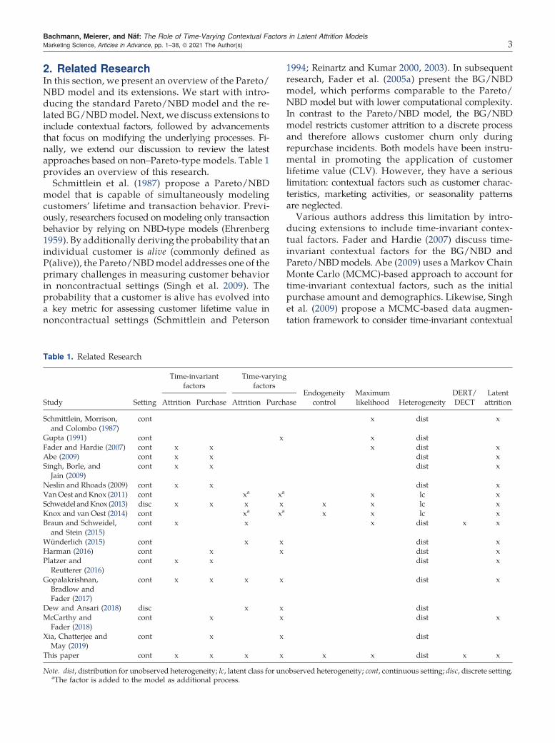
2. Related ResearchIn this section, we present an overview of the Pareto/NBD model and its extensions. We start with intro-ducing the standard Pareto/NBD model and the re-lated BG/NBDmodel. Next, we discuss extensions toinclude contextual factors, followed by advancementsthat focus on modifying the underlying processes. Fi-nally, we extend our discussion to review the latestapproaches based on non–Pareto-type models. Table 1provides an overview of this research.

Schmittlein et al. (1987) propose a Pareto/NBDmodel that is capable of simultaneously modelingcustomers’ lifetime and transaction behavior. Previ-ously, researchers focused onmodeling only transactionbehavior by relying on NBD-type models (Ehrenberg1959). By additionally deriving the probability that anindividual customer is alive (commonly defined asP(alive)), the Pareto/NBDmodel addresses one of theprimary challenges in measuring customer behaviorin noncontractual settings (Singh et al. 2009). Theprobability that a customer is alive has evolved intoa key metric for assessing customer lifetime value innoncontractual settings (Schmittlein and Peterson

1994; Reinartz and Kumar 2000, 2003). In subsequentresearch, Fader et al. (2005a) present the BG/NBDmodel, which performs comparable to the Pareto/NBD model but with lower computational complexity.In contrast to the Pareto/NBD model, the BG/NBDmodel restricts customer attrition to a discrete processand therefore allows customer churn only duringrepurchase incidents. Both models have been instru-mental in promoting the application of customerlifetime value (CLV). However, they have a seriouslimitation: contextual factors such as customer charac-teristics, marketing activities, or seasonality patternsare neglected.Various authors address this limitation by intro-

ducing extensions to include time-invariant contex-tual factors. Fader and Hardie (2007) discuss time-invariant contextual factors for the BG/NBD andPareto/NBDmodels. Abe (2009) uses a Markov ChainMonte Carlo (MCMC)-based approach to account fortime-invariant contextual factors, such as the initialpurchase amount and demographics. Likewise, Singhet al. (2009) propose a MCMC-based data augmen-tation framework to consider time-invariant contextual

Table 1. Related Research

Study Setting

Time-invariantfactors

Time-varyingfactors

Endogeneitycontrol

Maximumlikelihood Heterogeneity

DERT/DECT

LatentattritionAttrition Purchase Attrition Purchase

Schmittlein, Morrison,and Colombo (1987)

cont x dist x

Gupta (1991) cont x x distFader and Hardie (2007) cont x x x dist xAbe (2009) cont x x dist xSingh, Borle, and

Jain (2009)cont x x dist x

Neslin and Rhoads (2009) cont x x dist xVanOest andKnox (2011) cont xa xa x lc xSchweidel andKnox (2013) disc x x x x x x lc xKnox and van Oest (2014) cont xa xa x x lc xBraun and Schweidel,

and Stein (2015)cont x x x dist x x

Wünderlich (2015) cont x x dist xHarman (2016) cont x x dist xPlatzer and

Reutterer (2016)cont x x dist x

Gopalakrishnan,Bradlow andFader (2017)

cont x x x x dist x

Dew and Ansari (2018) disc x x distMcCarthy and

Fader (2018)cont x x dist x

Xia, Chatterjee andMay (2019)

cont x x dist

This paper cont x x x x x x dist x x

Note. dist, distribution for unobserved heterogeneity; lc, latent class for unobserved heterogeneity; cont, continuous setting; disc, discrete setting.aThe factor is added to the model as additional process.

Bachmann, Meierer, and Näf: The Role of Time-Varying Contextual Factors in Latent Attrition ModelsMarketing Science, Articles in Advance, pp. 1–38, © 2021 The Author(s) 3

factors when modeling latent customer attrition. How-ever, none of these extensions are able to model con-textual factors that vary over time.

Gupta (1991) is the first to introduce time-varyingcontextual factors to NBD-type models. However, incontrast to latent customer attrition models, NBD-type models focus only on customer purchases andneglect customer attrition. Recent extensions to latentcustomer attrition models include time-varying contex-tual factors for discrete and mixed noncontractualbusiness settings have been proposed. Schweidel andKnox (2013) present a discrete probabilistic latentattrition model, which captures the purchase processwith a discrete Bernoulli process and latent customerattrition with a Geometric distribution. The authorsfocus on time-discrete transactions in a charity set-ting, that is, whether a person has donated in a certainyear. Gopalakrishnan et al. (2017) present a vectorchangepointmodel in ahierarchicalBayesian frameworkto capture differences across a series of customer cohorts.Their approach allows for the probability of purchaseand attrition to vary by individual and time.

Another stream of research focuses on adding time-varying contextual factors to the transaction process.Building on the BG/NBD model (Fader et al. 2005a),Braun et al. (2015) propose an approach for incor-porating transaction-specific attributes. The authors’approach accounts for transaction characteristics atthe time of purchase as contextual factors. However,these characteristics remain constant after the trans-action and affect only the attrition process and notthe purchase process. The authors use the model toevaluate the impact of a customer’s service experienceat the time of purchase. Using a MCMC approach,Harman (2016) includes time-varying contextual factorsin the transaction process of the BG/NBD model.McCarthy and Fader (2018) develop an approach forcustomer-based corporate valuation in noncontrac-tual settings. The authors use a beta-geometric/mixed-log-normal model and allow time-varying contextualfactors to affect the purchase process.

A complementary stream of research modifies theunderlying processes to address issues caused byspecific contextual factors: Van Oest and Knox (2011)propose an extension of the BG/NBD model thatconsiders customer complaints by adding a thirdprocess to the customer purchase and attrition pro-cess of the standard model. Later, Knox and vanOest (2014) add the possibility for customer recov-ery after complaints. Wünderlich (2015) proposes thehierarchical Bayesian seasonal model with drop-out(HSMDO), which is capable of capturing individualand cross-sectional seasonality. The foundation forthis model is a discretely sampled inhomogeneousPoisson process with discrete periodic death op-portunities. Platzer and Reutterer (2016) propose an

extension of the Pareto/NBD model to describe reg-ularity patterns in purchase timing. They replace theNBD distribution with a mixture of gamma distribu-tions to allow for a varying degree of regularity acrosscustomers. The authors find empirical evidence on theimportance of the regularity of timing patterns acrossmultiple industries.Recently, non–Pareto-type models were proposed

as alternative approaches for customer base analysis.Dew and Ansari (2018) use a nonparametric frame-work for customer base analysis and propose theGaussian process propensity model (GPPM). Theauthors use Bayesian nonparametric Gaussian priorsto combine the latent functions of customer purchasebehavior and further include a latent function forcalendar-based time. Their model relies on a normalpopulation distribution to control for unobservedcustomer heterogeneity. Xia et al. (2019) apply deep-learning algorithms in the form of conditional re-stricted Boltzmann machines to predict customerpurchase patterns. Their approach does not distin-guish between purchases and attrition but rathermodels the customer’s purchase pattern as a whole.However, the model allows to include time-invariantand time-varying contextual factors, such as demo-graphics and marketing activities.

3. ModelOur approach builds on the Pareto/NBD model for con-tinuous noncontractual business settings (Schmittleinet al. 1987). To model time-varying contextual factors,we draw on Gupta (1991), who proposes an extensionto NBD-type models. Such models were widely usedin marketing research at this time (Jeuland et al. 1980,Schmittlein et al. 1985, Ehrenberg 1988). In contrast tolatent attrition models, NBD-type models do not takecustomer attrition into account and focus solely on thepurchase process.In the following, we explain how to include time-

varying contextual factors in the Pareto/NBD modelthat affect both the purchase and attrition rate. First,we introduce time-varying contextual factors into thepurchase process, and second, we introduce thesefactors into the customer attrition process. In bothcases, this will be achieved using a proportionalhazard approach. Third, we add both processes to asingle closed-form expression while also introducingcustomer heterogeneity to the two processes. Fourth,we derive the related expressions to determine theprobability that a customer is alive at the end of theestimation period (in previous studies sometimes alsonamed calibration period) (Schmittlein et al. 1987),the conditional expectation, and the discounted ex-pected conditional transactions (DECT; analogous tothe DERT proposed by Fader et al. 2005b, 2010). Fi-nally, we discuss model identification and propose


three generalized approaches to control for endoge-nous contextual factors. In this context, we also dis-cuss the impact of controlling for endogenous con-textual factors on predictive accuracy.

3.1. Purchase Process

Introducing time-varying contextual factors to thepurchase process consists of multiple steps. First,we build on the same assumptions as the standardPareto/NBD model, where customer purchases aremodeled according to a Poisson process with expo-nentially distributed interpurchase times. Second, weallow the purchase rate to be a function of the time-varying contextual factors and, therefore, also time.Next, to simplify all further derivations, we followGupta (1991) and assume that those contextual factorsare time invariant for a time interval of fixed length.Finally, we derive a general expression for the purchaseprocess. Later, we refer to these steps to facilitate abetter understanding of the model derivation. Wedenote variables specific for the purchase process withthe superscript P.

Without time-varying contextual factors being pres-ent, the purchase behavior of a customer i is modeledas a Poisson process with rate λi with regard to thenumber of purchases made during a specified timeinterval (i.e., the estimation period, (0, t]). It followsthat the probability of the number of purchases x in atime interval (0, t] is given by

P Y t( ) x( ) λit[ ]x

x!exp −λit[ ]. (1)

The probability of zero purchases for (1) defines thesurvivor function for the interpuchase time

P Y t( ) 0( ) SP t( ) exp −λit( ), (2)

and therefore, the density function for the inter-purchase time is given by

f P t( ) λi exp −λit( ). (3)

This corresponds to an exponentially distributed inter-purchase time for an individual customer.

To include time-varying contextual factors, we buildon theproportional hazardapproach.Thus,weallow thepurchase rate λi to be a function of the contextualfactors and therefore also of time:

λi t( ) λ0 exp γ′purchx

Pit

( ), (4)

where xPit denotes the vector of contextual factorsinfluencing the purchase process at time t, γpurch

represents a vector of contextual factor effect sizes, andλ0 is the base purchase rate. For simplicity, we assumeλ0 to be identical for all customers. This assumptionwill be relaxed later when customer heterogeneity is

introduced to the model. To simplify the notation, weremove the customer index i for all subsequent der-ivations. The coefficient γpurch may be directly inter-preted as rate elasticity. A 1% change in a contextualfactor xP changes the purchase rate by γ′

purchxP%. An

increase of the purchase rate corresponds to a de-crease in interpurchase time (Gupta 1991). Becauseλ(t) is now a function of time-varying contextual factors,the purchase process is now a nonhomogenous Poissonprocess (Ross 2014). In particular, the times betweenthe purchases of an individual customer are no longerindependent and identically distributed, except ifλ(t) λ. It follows that the probability of the numberof purchases x in a time interval (0, t] is given by (1)where we substitute λt by

θP0 t( )

∫ t

0λ τ( ) dτ. (5)

Note that (5) reduces to λt for a homogenous Poissonprocess. The survivor function and the density for theinterpurchase time are given as (2) and (3) with λtsubstituted by (5).In contrast to the standard Pareto/NBD model, the

timing of purchases becomes relevant when intro-ducing time-varying contextual factors. In particular,the interpurchase time between events j and j + 1mayhave a different distribution compared with the onebetween events j + 1 and j + 2. To account for this fact,we rewrite (1) using indices specifying the transac-tions. We denote for all subsequent derivations tj asthe time of transaction j with j 1, . . . , x and zj−1,j tj − tj−1 the time passed between transaction j − 1 and j.The probability of the number of purchases in a timeinterval (tj−1, tj] is then given by

P Y tj−1, tj( )

x( )

θPtj−1

zj−1,j( )[ ]x

x!exp −θP

tj−1zj−1,j( )[ ]

, (6)

with

θPtj−1

zj−1,j( )

∫ tj

tj−1

λ τ( ) dτ. (7)

With Zj−1,j as a random variable specifying the timebetween purchases j − 1 and j, we may derive thesurvivor function:

P Zj−1,j > zj−1,j|tj−1( )

P X tj−1, tj( )

0( )

exp −θPtj−1

zj−1,j( )[ ]

(8)

and arrive at the following density function of theinterpurchase time:

f P zj−1,j|tj−1( )

f P zj−1,j|z0,1, z1,2, . . . , zj−2,j−1( )

λ tj( )

exp −θPtj−1

zj−1,j( )[ ]

. (9)


Following Gupta (1991), we simplify θPtj−1

(t) by as-suming that the contextual factors are time-invariantfor time intervals of fixed length (e.g., one week).Therefore, the contextual factors change only fordifferent intervals while staying constant in between.In principle, these time intervals can be arbitrarilysmall. It is important to emphasize that while thetime-varying contextual factors are discretized, theunderlying purchase process remains continuous.In consequence, θP(t), will consist of multiple λ(t)components. We denote kj as the number of intervalssince purchase j − 1. Simplifying the notation, weindex the contextual factors as xP1 , . . . , x

Pkj. By doing so,

the factors are indexed relative to the purchases,where the interval count starts at one for every pur-chase. In particular, x1 specifies the contextual factorsin the interval that contains the (j − 1)th transaction,

whereas xkj specifies the ones in the interval of the jthtransaction. d1 is defined as the time of the transaction(j − 1) to the end of the first interval for any two suc-cessive transactions (j − 1) and j. Note that d1 is indexedrelative to the purchases. To illustrate the differentcomponents of θP

tj−1(t) in (7), let us outline three possible

cases. The different cases are illustrated in Figure 1.

Case 1. The two purchases that define the interpurchasetime occur during the same time interval (e.g., the firsttime interval),

λ t( ) λ1 λ0 exp γ′purchx

P1

( )

θPtj−1

t( )

∫ tj

tj−1

λ τ( ) dτ

∫ zj−1,j

0λ1 dτ

λ1zj−1,j.

Figure 1. Timeline of the Purchase Process Adapted from Gupta (1991)


Case 2. The two purchases that define the interpurchasetime occur in two consecutive time intervals (e.g., the firstand the second time interval),


P2

( )

θPtj−1

t( )

∫tj

tj−1

λ τ( ) dτ

∫d1+tj−1

tj−1

λ1 dτ +

∫tj

d1+tj−1

λ2 dτ

λ1d1 + λ2 zj−1,j − d1( )

.

Case 3. The two purchases that define the inter-purchase time occur in two nonconsecutive time in-tervals (e.g., the first and the third time interval),


P3

( )

θPtj−1

t( )

∫tj

tj−1

λ τ( ) dτ

∫d1+tj−1

tj−1

λ1 dτ

+

∫ 1+d1+tj−1

d1+tj−1

λ2 dτ +

∫tj

1+d1+tj−1

λ3 dτ

λ1d1 + λ2 + λ3 zj−1,j − d1 − 1( )

.

All further cases, with more time intervals betweenthe two purchase events, are composed in the samemanner. To derive a general expression for this pat-tern, we define

λ t( ) λ0 exp γ′purchx

Pl

( ), (10)

where l 1, . . . , kj denotes the interval in which t lies.It follows that λ(tj) λkj , and we arrive at a morepractical version of (7):

θPkjzj−1,j( )

λ1d1+∑kj−1

l2

λl+λkj zj−1,j−d1−δ kj−2( )[ ]

, (11)

where δ 0 if kj 1 and δ 1 if kj ≥ 2. δ accounts forthe special case, where two subsequent purchasesoccur within the same time interval. Substituting λ(t)and θP

kj(zj−1,j) from (10) and (11) into (8) and (9) pro-

vides the survivor and density functions with time-varying contextual factors. Remember that contextualfactors which are constant over time, result in a ho-mogeneous process (i.e., λ(t) λ and θ(t) λt).

Thus far, we have introduced time-varying con-textual factors into the purchase process. In the nextsection, we introduce time-varying contextual factorsinto the attrition process.

3.2. Attrition Process

To include time-varying contextual factors in theattrition process, we proceed analogously. AlthoughGupta (1991) introduces contextual factors to thepurchase process only, the underlying methodol-ogy is also applicable for the attrition process. In a

first step, we build on the assumption of the standardPareto/NBD model, where customer attrition is mod-eled by an exponential distribution. Next, we allow theattrition rate to be a function of the time-varying con-textual factors and then assume that those contextualfactors are time invariant for a time interval of fixedlength. Finally, we derive a general expression for theattrition process. The following discussion is structuredanalogously to the model derivation of the purchaseprocess. We denote variables specific for the attritionprocess with the superscript A.Without time-varying contextual factors being pres-

ent, the unobserved lifetime Ω of an individual cus-tomer is exponentially distributed. At the end of thislifetime, the customer is considered inactive. Thisleads to the following density and the survivor functionfor the attrition process:

fA ω( ) μi exp −μiω( )

, (12)

SAi ω( ) P Ω > ω( ) exp −μiω( )

, (13)

where μi is the attrition rate of an individual customer i.To compare the attrition process to the purchaseprocess, we can express attrition as a purchase-likeprocesswith two events for every customer: the initialtransaction is the first and a customer’s (unobserved)attrition is the second event. Therefore, the propertiesand derivations of the two processes are very similar.When including time-varying contextual factors,

the attrition rate becomes a function of the contextualfactors and of time:

μi ω( ) μ0 exp γ′attrx

Aiω

( ), (14)

where xAiω denotes the vector of contextual factorsinfluencing a customer’s attrition process during hislifetime ω. The variable γattr represents a vector ofeffect sizes for contextual factors. μ0 is the base at-trition rate. These contextual factors may or may notbe the same as xPit. Initially, we assume that μ0 is thesame for all customers. This assumption will be re-laxed later. The interpretation of the effect sizes γattr isidentical to the purchase process: a 1% change in acontextual factor xA changes the attrition rate byγ′attrx

A%. Again, we remove the customer index i in allsubsequent derivations to simplify the notation.Based on the density derived for the transaction

process (9), the density of a customer’s lifetime Ω isgiven by

f A ω( ) μ ω( ) exp −θA0 ω( )

[ ], (15)

where

θA0 ω( )

∫ω

0μ τ( ) dτ. (16)


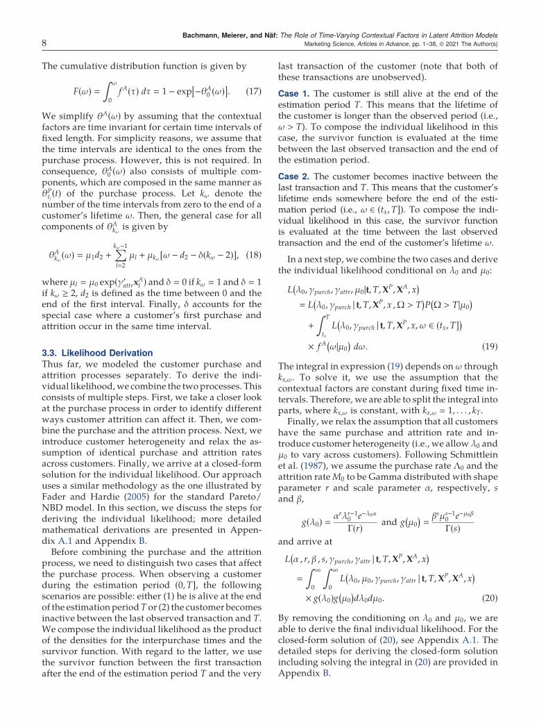
The cumulative distribution function is given by

F ω( )

∫ ω

0fA τ( ) dτ 1 − exp −θA

0 ω( )[ ]

. (17)

We simplify θA(ω) by assuming that the contextualfactors are time invariant for certain time intervals offixed length. For simplicity reasons, we assume thatthe time intervals are identical to the ones from thepurchase process. However, this is not required. Inconsequence, θA

0 (ω) also consists of multiple com-ponents, which are composed in the same manner asθPtj(t) of the purchase process. Let kω denote the

number of the time intervals from zero to the end of acustomer’s lifetime ω. Then, the general case for allcomponents of θA

kωis given by

θAkω

ω( ) μ1d2 +∑kω−1

l2

μl + μkω ω − d2 − δ kω − 2( )[ ], (18)

where μl μ0 exp(γ′attrx

Al ) and δ 0 if kω 1 and δ 1

if kω ≥ 2, d2 is defined as the time between 0 and theend of the first interval. Finally, δ accounts for thespecial case where a customer’s first purchase andattrition occur in the same time interval.

3.3. Likelihood Derivation

Thus far, we modeled the customer purchase andattrition processes separately. To derive the indi-vidual likelihood,we combine the two processes. Thisconsists of multiple steps. First, we take a closer lookat the purchase process in order to identify differentways customer attrition can affect it. Then, we com-bine the purchase and the attrition process. Next, weintroduce customer heterogeneity and relax the as-sumption of identical purchase and attrition ratesacross customers. Finally, we arrive at a closed-formsolution for the individual likelihood. Our approachuses a similar methodology as the one illustrated byFader and Hardie (2005) for the standard Pareto/NBD model. In this section, we discuss the steps forderiving the individual likelihood; more detailedmathematical derivations are presented in Appen-dix A.1 and Appendix B.

Before combining the purchase and the attritionprocess, we need to distinguish two cases that affectthe purchase process. When observing a customerduring the estimation period (0,T], the followingscenarios are possible: either (1) he is alive at the endof the estimation periodT or (2) the customer becomesinactive between the last observed transaction and T.We compose the individual likelihood as the productof the densities for the interpurchase times and thesurvivor function. With regard to the latter, we usethe survivor function between the first transactionafter the end of the estimation period T and the very

last transaction of the customer (note that both ofthese transactions are unobserved).

Case 1. The customer is still alive at the end of theestimation period T. This means that the lifetime ofthe customer is longer than the observed period (i.e.,ω > T). To compose the individual likelihood in thiscase, the survivor function is evaluated at the timebetween the last observed transaction and the end ofthe estimation period.

Case 2. The customer becomes inactive between thelast transaction and T. This means that the customer’slifetime ends somewhere before the end of the esti-mation period (i.e., ω ∈ (tx,T]). To compose the indi-vidual likelihood in this case, the survivor functionis evaluated at the time between the last observedtransaction and the end of the customer’s lifetime ω.

In a next step, we combine the two cases and derivethe individual likelihood conditional on λ0 and μ0:

L λ0, γpurch, γattr, μ0|t,T,XP,XA, x

( )

L λ0, γpurch | t,T,XP, x ,Ω > T

( )P Ω > T|μ0

( )

+

∫ T

tx

L λ0, γpurch | t,T,XP, x, ω ∈ tx,T( ]

( )

× fA ω|μ0

( )dω. (19)

The integral in expression (19) depends on ω throughkx,ω. To solve it, we use the assumption that thecontextual factors are constant during fixed time in-tervals. Therefore, we are able to split the integral intoparts, where kx,ω is constant, with kx,ω 1, . . . , kT.Finally, we relax the assumption that all customers

have the same purchase and attrition rate and in-troduce customer heterogeneity (i.e., we allow λ0 andμ0 to vary across customers). Following Schmittleinet al. (1987), we assume the purchase rate Λ0 and theattrition rateM0 to be Gamma distributed with shapeparameter r and scale parameter α, respectively, sand β,

g λ0( ) αrλr−1

0 e−λ0α

Γ r( )and g μ0

( )βsμs−1

0 e−μ0β

Γ s( )

and arrive at

L α , r, β , s, γpurch, γattr | t,T,XP,XA, x

( )

∫∞

0

∫∞

0L λ0, μ0, γpurch, γattr | t,T,X

P,XA, x( )

× g λ0( )g μ0

( )dλ0dμ0. (20)

By removing the conditioning on λ0 and μ0, we areable to derive the final individual likelihood. For theclosed-form solution of (20), see Appendix A.1. Thedetailed steps for deriving the closed-form solutionincluding solving the integral in (20) are provided inAppendix B.


3.4. P(alive)

In noncontractual settings, customer churn is notobserved. Therefore, the probability of being alive atthe end of the estimation period T, P(alive), is a keycomponent of predicting future purchase behavior.P(alive) is the probability that the lifetime of thecustomer is larger than T, P(Ω > T), given all availableinformation. To obtain P(alive), we first apply theBayes’ theorem to obtain the posterior probability ofbeing alive. Because the purchase rate λ0 and theattrition rate μ0 are not directly observed, we furtherneed to include the posterior distribution of (λ0, μ0),before we can integrate them out and arrive at theclosed-form solution for P(alive).

Applying Bayes’ theorem to the individual likeli-hood (19) results in

P Ω > T|λ0, μ0,XP,XA, γpurch, γattr, x, t,T

( )

L λ0, γpurch|X

P, x, t,T,Ω > T( )

P Ω > T|μ0

( )

L λ0, γpurch, γattr, μ0|t,T,XP,XA, x( ) . (21)

Because the purchase rate λ0 and the attrition rate μ0

are not directly observed, we multiply (21) by theposterior distribution of (λ0, μ0), which is given as

g λ0, μ0|r, α, s, β, γpurch, γattr,XP,XA, x, t,T

( )

L λ0, γpurch, γattr, μ0|X

P,XA, x, t,T( )

g λ0( )g μ0

( )

L α, r, β, s, γpurch, γattr|XP,XA, x, t,T

( ) .

(22)

Then, we take the integral with respect to this jointdistribution to obtain the final P(alive) expression:

P Ω > T|r, α , s, β , γpurch, γattr,XP,XA, x, t,T

( )

∫∞

0

∫∞

0P Ω > T|λ0, μ0,X

P,XA, γpurch, γattr, x, t,T( )

× g λ0, μ0|r, α , s, β , γpurch, γattr,XP,XA, x, t,T

( )

× dλ0dμ0. (23)

The closed-form solution to (23) is reported inAppendix A.2, and related derivations are reportedin Appendix C.

3.5. Conditional Expectation

The conditional expectation metric allows practi-tioners and researchers to predict the future numberof purchases of an individual given a customer’s pastpurchase behavior. To derive the expression, wefollow multiple steps. We start with the assumptionthat the customer did not stop purchasing before theprediction period. However, we still have to distin-guish two cases for a customer’s possible attritionduring the prediction period. We use the character-istics of nonhomogenous Poisson processes and the

fact that the contextual factors are assumed to be timeinvariant for an interval of fixed length to derive thefirst conditional expectation. Last, we relax our initialassumption and allow attrition before the predictionperiod. In this section, we discuss the steps for de-riving the conditional expectation; more mathemat-ical derivations are presented in Appendix C.We start by deriving E[Y(T,T + t)|r, α, s , β, γpurch,

γattr,XP,XA, x, t,T], where Y(T,T + t) is a random var-

iable specifying the number of purchases made afterthe estimation period in the interval (T,T + t]. Our ap-proach is based on Fader and Hardie (2005). We startderiving the conditional expectation under the as-sumption that the customer is alive after the end of theestimation period T. This assumption is relaxed later.Under this assumption, the conditional expectationis a special case of the purchase process, where wehave two transactions, the first one at T and thesecond one at ω, with ω ∈ (T,T + t].Although we assume that all customers are alive at

the end of the estimation period, there are still twodifferent cases to consider about the timing of cus-tomer attrition. The customer may stop buying afterthe end of the prediction period or during the pre-diction period.

Case 1. The lifetime of the customer is longer than theprediction period, that is, ω > T + t. In this case, we getthe expectation of the nonhomogenous purchase pro-cess with ω > T + t:

E Y T,T + t( )|λ0,XP, γpurch,Ω > T + t

[ ].

Case 2. The customer stops purchasing betweenthe end of the observation period and the end ofthe prediction period. In this case, we get the ex-pectation of the nonhomogenous attrition processwith ω ∈ (T,T + t]:

E Y T,T + t( )|λ0,XP, γpurch,Ω ∈ T,T + t( ]

[ ].

We combine the two cases, but because we do notobserve the customer lifetime ω, we also have toconsider the attrition process:

E Y T,T + t( )|λ0, μ0,XP,XA, γpurch, γattr,Ω > T

[ ]


[ ]

× P Ω > T + t|μ0,Ω > T( )

+

+

∫ T+t

TE Y T,T + t( )|λ0,X

P, γpurch,[(

ω ∈ T,T + t( ]])

× fA ω|μ0,Ω > T( )

dω. (24)

For expression (24), we assume that customers are aliveat the end of the observation period T, that is, ω > T.


To relax this assumption, we add the posterior distri-butionof being alive atT, P(alive), fromEquation (A.2).

E Y T,T + t( )|λ0, μ0,XP,XA, γpurch, γattr, x, t,T

[ ]

E Y T,T + t( )|λ0, μ0,XP,XA, γpurch, γattr,

[x, t,Ω > T

]

× P Ω > T|λ0, μ0,XP,XA, γpurch, γattr, x, t,T

( ). (25)

By removing the conditioning on λ0 and μ0, we arriveat the closed-form solution reported in Appendix A.3.

3.6. DECT

To estimate individual customer lifetime values withthe proposed model in combination with a Gamma/Gamma model (Colombo and Jiang 1999, Fader et al.2005b), we need to derive the present value of the ex-pected future transactions and account for the discountrate. We define the DECT. The concept of this metricis very similar to the discounted expected residualtransactions (DERT) (Fader et al. 2005b, 2010).

The general formulation of the customer lifetimevalue (CLV) is

E CLV( )

∫∞

0

v t( )S t( )d t( )dt,

where v(t) is the customer value at t, S(t) 1 − F(t) P(Ω > t) denotes the survivor function ofΩ and d(t) aspecific discount factor. Assuming that the value ofeach transaction remains constant, v(t) can be factoredout leaving only the purchase rate λ(t) in the integral:

∫∞

0λ t( )S t( )d t( )dt.

These are the discounted expected transactions (DETs).Starting instead at t T, the end of the estimation

period, for continuous discounting with a rate of ∆,gives the DERT (Fader et al. 2005b, 2010):

DERT ∆|λ0, μ0,XP,XA, γpurch, γattr,Ω > T

( )

∫∞

T

λ t( )P Ω > t|Ω > T( )d t( )dt

∫∞

Tλ0 exp xPt

( )exp −μ0 θ0 t( ) −θ0 T( )( )

[ ]

× exp −∆ t−T( )[ ]dt.

Whenmodeling time-varying contextual factors, we facethe issue that the measurements of the time-varyingcontextual factors are likely not known up to infinity.Thus, we make predictions only within a time frame forwhich the time-varying contextual factors are known.Therefore, we truncate the time horizon of our predic-tions and approximate the DERT as DECT:

DECT ∆, t|r, α, s , β, γpurch, γattr,XP,XA, x, t,T

( )

∫ T+t

Tλ0 exp xPτ

( )exp −μ0 θ0 τ( ) − θ0 T( )( )

[ ]

× exp −∆ τ − T( )[ ] dτ, (26)

where t > 0 is theprediction length.Wepresent theclosed-form solution to the integral in (26) in Appendix A.4.

3.7. Model Identification

When considering contextual factors in the Pareto/NBDmodel,model identification has to be addressed.In the following, we focus on the ability of the ex-tended Pareto/NBD model to separately identify theeffects of time-varying contextual factors on the pur-chase process and the attrition process. The identifica-tion of standard latent customer attrition models with-out contextual factors has been thoroughly discussed inprior studies (Schmittlein et al. 1987, Fader andHardie2005, Schweidel and Knox 2013).First, we describe the effects of contextual factors:

modeling contextual effects means that a part of theunobserved heterogeneity is substituted by system-atic differences, which are expressed by the contex-tual factors. As such, the parameter r, whichmeasureshomogeneity in the purchase process, and the pa-rameter s, which measures homogeneity in the attritionprocess, should increase when modeling contextual ef-fects (Gupta 1991). The effects of contextual factors mayinfluence both the purchase and the attrition processes,just one of the processes, or neither of the processes.Although this applies to both time-invariant and time-varying contextual factors, the identification of these twocategories of contextual effects relies on different sourcesof variation.To identify time-invariant contextual factors, it is

possible to leverage the variation across customergroups. For example, female customers might pur-chase more. However, their loyalty is the same as thatof male customers. Thus, gender will influence onlythe purchase process and not the attrition process.Another example is that older customers might bemore loyal to the retailer, and, therefore, more timemust pass until they stop purchasing. However, theirpurchase rate may be the same as that of youn-ger customers.The identification of time-varying contextual fac-

tors, which allow us to capture the effects of dynamicchanges in a customer’s context (e.g., personalizedmarketing), is more complex. Individual customersare allowed to change their purchase and attritionbehavior over time. Temporal events may cause astrictly temporary change in the purchase rate (e.g.,shortly after receiving a personalized marketing of-fer, customers tend to purchasemore). However, suchan event may also influence a customer’s futurepurchase behavior. For example, personalized mar-keting might encourage customers to return to thestore in the future and therefore can reduce thelikelihood that a customerwill stop purchasing at thispoint in time. To identify such patterns, variationacross time must be considered.


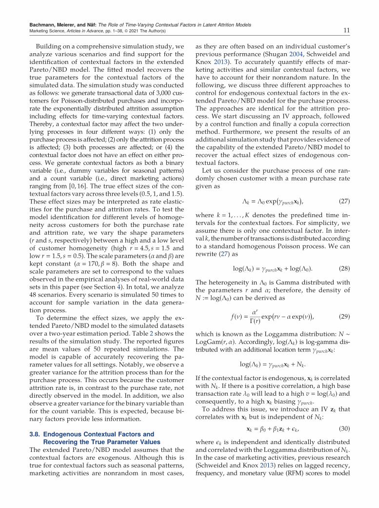
Building on a comprehensive simulation study, weanalyze various scenarios and find support for theidentification of contextual factors in the extendedPareto/NBD model. The fitted model recovers thetrue parameters for the contextual factors of thesimulated data. The simulation study was conductedas follows: we generate transactional data of 3,000 cus-tomers for Poisson-distributed purchases and incorpo-rate the exponentially distributed attrition assumptionincluding effects for time-varying contextual factors.Thereby, a contextual factor may affect the two under-lying processes in four different ways: (1) only thepurchase process is affected; (2) only the attrition processis affected; (3) both processes are affected; or (4) thecontextual factor does not have an effect on either pro-cess. We generate contextual factors as both a binaryvariable (i.e., dummy variables for seasonal patterns)and a count variable (i.e., direct marketing actions)ranging from [0, 16]. The true effect sizes of the con-textual factors vary across three levels (0.5, 1, and 1.5).These effect sizes may be interpreted as rate elastic-ities for the purchase and attrition rates. To test themodel identification for different levels of homoge-neity across customers for both the purchase rateand attrition rate, we vary the shape parameters(r and s, respectively) between a high and a low levelof customer homogeneity (high r 4.5, s 1.5 andlow r 1.5, s 0.5). The scale parameters (α and β) arekept constant (α 170, β 8). Both the shape andscale parameters are set to correspond to the valuesobserved in the empirical analyses of real-world datasets in this paper (see Section 4). In total, we analyze48 scenarios. Every scenario is simulated 50 times toaccount for sample variation in the data genera-tion process.

To determine the effect sizes, we apply the ex-tended Pareto/NBD model to the simulated datasetsover a two-year estimation period. Table 2 shows theresults of the simulation study. The reported figuresare mean values of 50 repeated simulations. Themodel is capable of accurately recovering the pa-rameter values for all settings. Notably, we observe agreater variance for the attrition process than for thepurchase process. This occurs because the customerattrition rate is, in contrast to the purchase rate, notdirectly observed in the model. In addition, we alsoobserve a greater variance for the binary variable thanfor the count variable. This is expected, because bi-nary factors provide less information.

3.8. Endogenous Contextual Factors and

Recovering the True Parameter Values

The extended Pareto/NBD model assumes that thecontextual factors are exogenous. Although this istrue for contextual factors such as seasonal patterns,marketing activities are nonrandom in most cases,

as they are often based on an individual customer’sprevious performance (Shugan 2004, Schweidel andKnox 2013). To accurately quantify effects of mar-keting activities and similar contextual factors, wehave to account for their nonrandom nature. In thefollowing, we discuss three different approaches tocontrol for endogenous contextual factors in the ex-tended Pareto/NBD model for the purchase process.The approaches are identical for the attrition pro-cess. We start discussing an IV approach, followedby a control function and finally a copula correctionmethod. Furthermore, we present the results of anadditional simulation study that provides evidence ofthe capability of the extended Pareto/NBD model torecover the actual effect sizes of endogenous con-textual factors.Let us consider the purchase process of one ran-

domly chosen customer with a mean purchase rategiven as

Λk Λ0 exp γpurchxk( )

, (27)

where k 1, . . . ,K denotes the predefined time in-tervals for the contextual factors. For simplicity, weassume there is only one contextual factor. In inter-val k, thenumberof transactions isdistributedaccordingto a standard homogenous Poisson process. We canrewrite (27) as

log Λk( ) γpurchxk + log Λ0( ). (28)

The heterogeneity in Λ0 is Gamma distributed withthe parameters r and α; therefore, the density ofN : log(Λ0) can be derived as

f ν( ) αr

Γ r( )exp rν − α exp ν( )

( ), (29)

which is known as the Loggamma distribution: N ∼LogGam(r, α). Accordingly, log(Λk) is log-gamma dis-tributed with an additional location term γpurchxk:

log Λk( ) γpurchxk +Nk.

If the contextual factor is endogenous, xk is correlatedwith Nk. If there is a positive correlation, a high basetransaction rate λ0 will lead to a high v log(λ0) andconsequently, to a high xk biasing γpurch.To address this issue, we introduce an IV zk that

correlates with xk but is independent of Nk:

xk β0 + β1zk + ǫk, (30)

where ǫk is independent and identically distributedand correlatedwith the Loggammadistribution ofNk.In the case of marketing activities, previous research(Schweidel and Knox 2013) relies on lagged recency,frequency, and monetary value (RFM) scores to model


a firm’s targeting decision. This leads us to the fol-lowing two-step approach: first, we estimate (30) usingleast squares to obtain xk : β0 + β1zk. Second, weestimate the extended Pareto/NBD model, but in-stead of using the endogenous contextual factor xk, weuse xk. The procedure is similar for the attritionprocess. The proposed two-step IV approach assumesa linear combination of the explanatory variables

(i.e., linear-in-parameters model). A second methodto control for endogenous variables is the controlfunction approach (Rivers and Vuong 1988, Petrinand Train 2010). It offers a parsimonious way to ac-count for endogeneity of a contextual factor even if itinteractswith other exogenous variables (Wooldridge2015). Instead of estimating the extended Pareto/NBD model with xk, we add the error term ǫk in (30)

Table 2. Simulation Results for Recovering Exogenous Contextual Factors

Contextualfactor type Homogeneity

True valueγpurch

Meanestimateγpurch

Estimate SDγpurch

True valueγattr

Meanestimateγattr

EstimateSD γattr

Contextual factor influences Binary High 0.5 0.516 0.081 0.5 0.555 0.135both processe Binary High 1 0.989 0.072 1 0.990 0.149

Binary High 1.5 1.473 0.074 1.5 1.538 0.118Binary High 0.5 0.482 0.106 1.5 1.539 0.149Binary High 1.5 1.488 0.065 0.5 0.518 0.060Binary Low 0.5 0.488 0.070 0.5 0.506 0.241Binary Low 1 0.998 0.066 1 0.968 0.285Binary Low 1.5 1.509 0.073 1.5 1.439 0.312Binary Low 0.5 0.516 0.085 1.5 1.462 0.313Binary Low 1.5 1.516 0.070 0.5 0.553 0.209Count High 0.5 0.516 0.045 0.5 0.527 0.071Count High 1 1.006 0.043 1 1.043 0.071Count High 1.5 1.436 0.019 1.5 1.483 0.089Count High 0.5 0.480 0.095 1.5 1.452 0.114Count High 1.5 1.433 0.029 0.5 0.506 0.058Count Low 0.5 0.480 0.095 0.5 1.452 0.114Count Low 1 0.999 0.033 1 0.975 0.120Count Low 1.5 1.454 0.028 1.5 1.429 0.092Count Low 0.5 0.496 0.051 1.5 1.450 0.157Count Low 1.5 1.454 0.019 0.5 0.492 0.087

Contextual factor influences Binary High 0.5 0.488 0.065 0 0.002 0.125only purchase process Binary High 1 1.018 0.066 0 −0.002 0.108

Binary High 1.5 1.508 0.063 0 0.032 0.093Binary Low 0.5 0.512 0.072 0 0.056 0.179Binary Low 1 0.999 0.061 0 0.011 0.227Binary Low 1.5 1.500 0.051 0 −0.017 0.186Count High 0.5 0.507 0.040 0 0.020 0.083Count High 1 0.995 0.028 0 0.023 0.067Count High 1.5 1.414 0.018 0 0.016 0.057Count Low 0.5 0.505 0.039 0 0.004 0.163Count Low 1 0.964 0.023 0 0.005 0.094Count Low 1.5 1.449 0.019 0 −0.024 0.095

Contextual factor influences Binary High 0 −0.008 0.111 0.5 0.528 0.172only attrition process Binary High 0 0.021 0.102 1 1.012 0.174

Binary High 0 −0.039 0.121 1.5 1.467 0.179Binary Low 0 0.007 0.095 0.5 0.054 0.261Binary Low 0 0.002 0.085 1 0.925 0.271Binary Low 0 −0.006 0.098 1.5 1.451 0.345Count High 0 0.006 0.066 0.5 0.507 0.077Count High 0 −0.002 0.095 1 0.984 0.117Count High 0 −0.046 0.136 1.5 1.486 0.129Count Low 0 −0.006 0.052 0.5 0.472 0.193Count Low 0 0.014 0.061 1 1.013 0.178Count Low 0 0.005 0.067 1.5 1.421 0.212

No influence Count High 0 0.001 0.059 0 0.002 0.102Count Low 0 0.010 0.050 0 0.058 0.161Binary High 0 −0.007 0.080 0 −0.009 0.100Binary Low 0 0.018 0.091 0 0.068 0.268


as an additional contextual factor, to the model (inaddition to the endogenous contextual factor).

A third approach that can be used to control forendogenous variables is based on the copula correc-tion method proposed by Park and Gupta (2012).Similar to control function approach, this approachadds a factor to the model. However, this additionalfactor is derived using a Gaussian copula and themarginal distribution of the endogenous factor. Thismeans, in addition to the endogenous contextual fac-tor xk, we add the contextual factor p∗k , where

p∗k Φ−1 H xk( )( ), (31)

with H(xk) as the marginal distribution of the en-dogenous regressor andΦ−1 as the inverse cumulativedistribution function of a standard normal distribu-tion. Including the marginal distribution of the en-dogenous contextual factors solves the correlationbetween the endogenous contextual factor and thestructural error and therefore results in consistentparameter estimates. Although it is more complex,the copula correction method has two key advan-tages: (1) there is no need to add an instrumentalvariable as all required information is extracted fromthe already available data and (2) it is applicable todiscrete endogenous variables. A drawback of thecopula approach is the possibility of introducingmulticollinearity to the model, which may affect modelconvergence. To ensure identification, the discrete en-dogenous contextual factor must not be binomiallydistributed (Park and Gupta 2012).

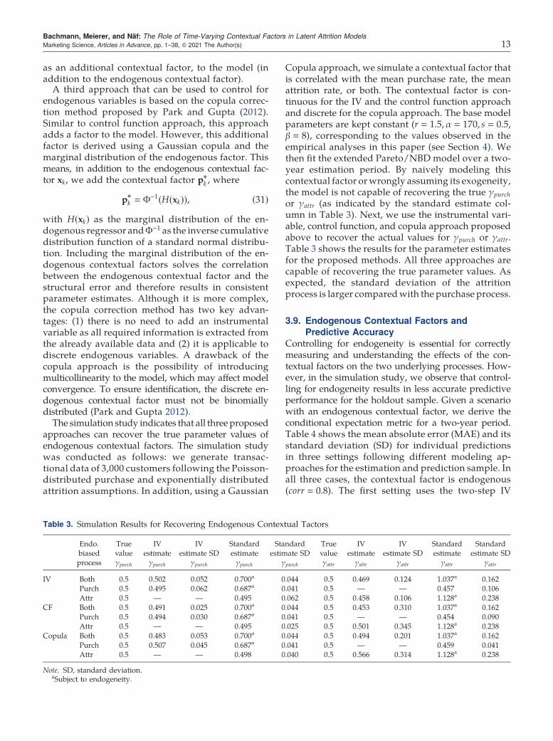
The simulation study indicates that all three proposedapproaches can recover the true parameter values ofendogenous contextual factors. The simulation studywas conducted as follows: we generate transac-tional data of 3,000 customers following the Poisson-distributed purchase and exponentially distributedattrition assumptions. In addition, using a Gaussian

Copula approach, we simulate a contextual factor thatis correlated with the mean purchase rate, the meanattrition rate, or both. The contextual factor is con-tinuous for the IV and the control function approachand discrete for the copula approach. The base modelparameters are kept constant (r 1.5, α 170, s 0.5,β 8), corresponding to the values observed in theempirical analyses in this paper (see Section 4). Wethen fit the extended Pareto/NBD model over a two-year estimation period. By naively modeling thiscontextual factor orwrongly assuming its exogeneity,the model is not capable of recovering the true γpurch

or γattr (as indicated by the standard estimate col-umn in Table 3). Next, we use the instrumental vari-able, control function, and copula approach proposedabove to recover the actual values for γpurch or γattr.Table 3 shows the results for the parameter estimatesfor the proposed methods. All three approaches arecapable of recovering the true parameter values. Asexpected, the standard deviation of the attritionprocess is larger comparedwith the purchase process.

3.9. Endogenous Contextual Factors and

Predictive Accuracy

Controlling for endogeneity is essential for correctlymeasuring and understanding the effects of the con-textual factors on the two underlying processes. How-ever, in the simulation study, we observe that control-ling for endogeneity results in less accurate predictiveperformance for the holdout sample. Given a scenariowith an endogenous contextual factor, we derive theconditional expectation metric for a two-year period.Table 4 shows the mean absolute error (MAE) and itsstandard deviation (SD) for individual predictionsin three settings following different modeling ap-proaches for the estimation and prediction sample. Inall three cases, the contextual factor is endogenous(corr 0.8). The first setting uses the two-step IV

Table 3. Simulation Results for Recovering Endogenous Contextual Tactors

Endo.biasedprocess

Truevalueγpurch

IVestimateγpurch

IVestimate SD

γpurch

Standardestimateγpurch

Standardestimate SD

γpurch

Truevalueγattr

IVestimateγattr

IVestimate SD

γattr

Standardestimateγattr

Standardestimate SD

γattr

IV Both 0.5 0.502 0.052 0.700a 0.044 0.5 0.469 0.124 1.037a 0.162Purch 0.5 0.495 0.062 0.687a 0.041 0.5 — — 0.457 0.106Attr 0.5 — — 0.495 0.062 0.5 0.458 0.106 1.128a 0.238

CF Both 0.5 0.491 0.025 0.700a 0.044 0.5 0.453 0.310 1.037a 0.162Purch 0.5 0.494 0.030 0.687a 0.041 0.5 — — 0.454 0.090Attr 0.5 — — 0.495 0.025 0.5 0.501 0.345 1.128a 0.238

Copula Both 0.5 0.483 0.053 0.700a 0.044 0.5 0.494 0.201 1.037a 0.162Purch 0.5 0.507 0.045 0.687a 0.041 0.5 — — 0.459 0.041Attr 0.5 — — 0.498 0.040 0.5 0.566 0.314 1.128a 0.238

Note. SD, standard deviation.aSubject to endogeneity.


approach to correct for endogenous contextual factorsfor the model estimation, but no IV is used to predictcustomer behavior during the holdout period. In thesecond setting, we control for endogenous contextualfactors during both model estimation and prediction.In the third setting, we naively use the endogenousfactor to estimate the model and predict customerbehavior, that is, we do not control for endogeneity.The prediction period is two years. We observe thatthe setting that does not control for endogenouscontextual factors outperforms the other two ap-proaches. These findings are in line with those inEbbes et al. (2011). Consistent with these authors, wesuggest that researchers carefully think about theirkey model objective and thus decide whether con-trolling for endogenous contextual factors is advis-able in their specific research context. Although it israrely advisable if the study’s focus is primarilypredictive modeling, controlling for endogeneity is ofutmost importance if the study’s focus is on disen-tangling causal relationships.

4. Empirical AnalysisWe use three real-world data sets from the retailingindustry to test the extended Pareto/NBDmodel. Thefirst data set is from amultichannel catalogmerchant,the second data set is from an electronic retailer, andthe third data set is from a sporting goods retailer. Thefirst two data sets are publicly available.

Although all three datasets are from the retailingindustry, they have distinct characteristics that relateto commonly observed scenarios across various in-dustry groups. First, the nature of available time-varying contextual factors differs across firms. Somefirms can rely on detailed information about contex-tual factors for individual customers. This is not thecase for other firms, which either do not store suchrecords or are not allowed to use them for customerbase analyses, for example, because of data privacyregulations. Second, customer transactions across firmsare characterized by varying interpurchase times. Al-though some firms record multiple transactions forindividual customers eachmonth, the time between thetransactions of individual customers is considerablylonger for other firms. To account for these varyingcharacteristics, we analyze data sets that include threecommonly observed scenarios in this context. The firstdata set corresponds to the scenario where firms have

access to a wide set of contextual factors for each in-dividual and at the aggregate level. Furthermore, thetransactions for customers occur rather frequently. Thesecond data set is widely comparable to the first dataset, but information on contextual factors is limited.This means that information is only available foraggregate-level time varying contextual factors. Ad-ditionally, interpurchase times are longer than those inthe first data set. The third data set again includesinformation on both individual and aggregate-levelcontextual factors and is characterized by longer inter-purchase times. Analyzing multiple datasets facilitatesa more robust discussion of when and how modelingcontextual factors contribute to increasing the pre-dictive accuracy of latent probabilistic customer at-trition models.First, we compare our extended Pareto/NBDmodel,

which includes time-varying and time-invariant con-textual factors, with the standard Pareto/NBDmodel,which does not account for any contextual factors. Wecompare the parameter estimates and the in-sampleperformance of these two models. To evaluate the in-sample performance during the estimation period, weuse the Bayesian information criteria (BIC) and the log-likelihood (LL) values. Because these two models arenested, the parameters and LL values are directlycomparable. Second, for the customer base analysis,we benchmark the out-of-sample predictive perfor-mance at the individual and aggregate level andcompare it with that of the standard Pareto/NBDmodel and four state-of-the-art models. We compareit with that of the pareto/GGG model (Platzer andReutterer 2016), which is the latest published Pareto-typemodel, and the transaction attributemodel (TAM),which was introduced by Braun et al. (2015). More-over, we apply the GPPM, a Bayesian nonparametricframework proposed by Dew and Ansari (2018),which is the latest published non–Pareto-type ap-proach used for customer base analysis. Finally, webenchmark it against the latent attrition model withdirect marketing activities (LAMDMA) proposed bySchweidel and Knox (2013). The parameter estimatesare obtained either by maximum likelihood estima-tion or by using a MCMC-based approach in accor-dance with the original studies. Comparisons aremade for each of the three datasets. To evaluate out-of-sample performance at the individual level, we usethe mean absolute error (MAE) and the correlation

Table 4. Simulation Results for Predictive Accuracy with Endogenous Contextual Factors

Two-year prediction period MAE Standard deviation of MAE

Approach used IV only during estimation 0.347 0.107Approach used IV during estimation and prediction 0.130 0.020Approach did not use IV 0.125 0.010


between the predicted and observed number of trans-actions for the individual customers. The MAE is basedon the absolute difference between the predictednumber of transactions and the observed transac-tions up to the specified time point for every cus-tomer. We report the mean of these errors acrossindividual customers. Similarly, the individual-levelcorrelation measures the relationship between thepredicted number of transactions and the observednumber of transactions of individual customers up tothe specified time point. We use the conditional ex-pectation metric. To examine the robustness of ourfindings, we assess the predictive accuracy of themodels for different prediction periods. Furthermore,we compare model performance in terms of identifyingthe future best 10% and 20% of customers (Wübben andWangenheim 2008). We measure MAE at the aggre-gate level for both the predicted and observedweeklycumulative transactions.

4.1. Multichannel Catalog Merchant

The first data set is from a multichannel catalogmerchant. We analyze the purchase history of 1,402customers who made a purchase for the first timebetween January 2005 andMarch 2005. The data set ispublicly available from Marketing EDGE (MarketingEDGE 2013). The customer cohort accounts for 2,929transactions between January 2005 and September2012. A transaction record consists of the purchasedate and customer ID. Table 5 summarizes the keydescriptive statistics. We fit the models based onrepeated transactions during a one-year estimationperiod and examine the predictive performance of allfour models based on different prediction periods.

In the Extended Pareto/NBD model, we considerthree contextual factors: (1) catalog mailings, (2) sea-sonal purchase patterns, and (3) acquisition channels.Although the first two contextual factors are timevarying on a weekly basis, the last is time invariant,that is, does not change over time. Customers receivemultiple catalogs by mail every year, with timingof these mailings differing across customers. Catalogmailings are sent to the customers irrespective of theirprevious purchase histories. We include catalog mail-ings as an individual-level time-varying contextual

factor in the extended Pareto/NBD model. Thevariable is operationalized as a dummy variable. Fur-thermore, like many retailing companies, this multi-channel merchant is subject to seasonal purchase pat-terns. During the Christmas season, the firm observes asignificant increase in purchases, for example. We in-clude the seasonal pattern as a time-varying contextualfactor at the aggregate level, that is, although varyingover time, this contextual factor is the same for all cus-tomers. The information on high season is derived fromhistorical data and expert knowledge. Finally, we dis-tinguish between online and offline customers and in-clude the first-purchase channel for every customer as atime-invariant contextual factor.Our results show that the extended Pareto/NBD

model has a better in-sample fit in terms of the LL andBIC. The parameter estimates andmodel fit are shownin Table 6. The frequency plot of repeat transactionsin Figure 2 indicates a good in-sample fit. Becauseheterogeneity in the data are captured by Gammadistributions, the parameters r and s are direct mea-sures of the extent of heterogeneity in customers’purchase and attrition rates, respectively. The higherthe value of parameter r, the higher the homogene-ity in the purchase process, and the higher the valueof parameter s, the higher the homogeneity in theattrition process (Gupta 1991). Explicitly modelingcontextual factors in the extended Pareto/NBD modelexplains unobserved heterogeneity among customers.In the extended Pareto/NBD,we observe higher valuesfor r and s, indicating more homogeneity among cus-tomers for both processes.The coefficients of the contextual factors may be

directly interpreted as rate elasticity. A 1% change in acontextual factor XP or XA changes the purchase orattrition rates by γpurchX

P or γattrXA%, respectively

(Gupta 1991). Every contextual factor has two coeffi-cients. While the first coefficient represents the influenceon the transaction rate, the second coefficient representsthe effects on the customer’s lifetime. The coefficients ofthe contextual factors suggest that (1) seasonal pat-terns increase purchase levels but do not significantlyaffect customer attrition and (2) the first-purchasechannel does not significantly affect purchase levels,but the customers acquired online churn faster.

Table 5. Descriptive Statistics for the Multichannel Catalog Merchant Data Set

Three-month cohort Estimation period Holdout period Total

Sample size — — 1,402Available timeframe and split 1 year 6.7 years 7.7 yearsAverage number of purchases per customer 1.242 2.682 2.089Standard deviation of repeated purchases 0.619 2.202 2.449Number of purchases 1741 1188 2929Zero repeaters 1156 959 850


Table 7 compares the aggregate and individual out-of-sample performance of the extended Pareto/NBDmodel with that of the standard Pareto/NBD model,the TAM, the Pareto/GGGmodel, the GPPM, and theLAMDMA based on the future level of transactions

(conditional expectation). The extended Pareto/NBDmodel outperforms all other models at the individ-ual and aggregate level except for the aggregateone-year prediction of the GPPM. The TAM andLAMDMA do not fulfill the Karush-Kuhn-Tucker

Table 6. Parameter Estimates for the Multichannel Catalog Merchant Data Set

Extended Pareto/NBD

Standard Pareto/NBD Description

LL value −2,025.322 −2,056.098BIC 4,123.100 4,141.178r 1.548* 1.137* Homogeneity (purchase process)α 174.482* 108.174** Scale parameter (purchase process)s 0.531 0.181*** Homogeneity (attrition process)β 8.954 0.373 Scale parameter (attrition)γpurch, 1 0.194 — Direct marketing (purchase process)γpurch, 2 0.821*** — Seasonality (purchase process)γpurch, 3 0.210 — Channel (purchase process; online = 1, offline = 0)γattr, 1 −5.131 — Direct marketing (attrition process)γattr, 2 −0.132 — Seasonality (attrition process)γattr, 3 1.907** — Channel (attrition process; online = 1, offline = 0)

*p < 0.05; **p < 0.01; ***p < 0.001.

Figure 2. In- and Out-Sample Performance for the Multichannel Catalog Merchant Data Set


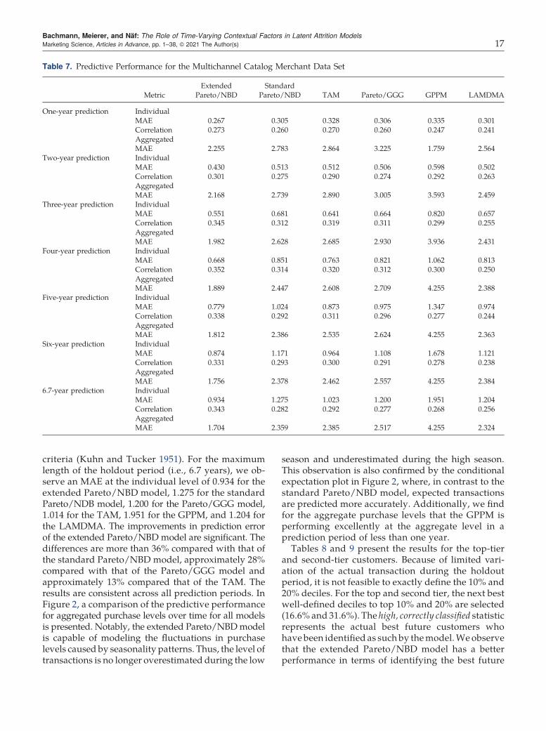
criteria (Kuhn and Tucker 1951). For the maximumlength of the holdout period (i.e., 6.7 years), we ob-serve an MAE at the individual level of 0.934 for theextended Pareto/NBD model, 1.275 for the standardPareto/NDB model, 1.200 for the Pareto/GGG model,1.014 for the TAM, 1.951 for the GPPM, and 1.204 forthe LAMDMA. The improvements in prediction errorof the extended Pareto/NBD model are significant. Thedifferences are more than 36% compared with that ofthe standard Pareto/NBD model, approximately 28%compared with that of the Pareto/GGG model andapproximately 13% compared that of the TAM. Theresults are consistent across all prediction periods. InFigure 2, a comparison of the predictive performancefor aggregated purchase levels over time for all modelsis presented. Notably, the extended Pareto/NBDmodelis capable of modeling the fluctuations in purchaselevels caused by seasonality patterns. Thus, the level oftransactions is no longer overestimated during the low

season and underestimated during the high season.This observation is also confirmed by the conditionalexpectation plot in Figure 2, where, in contrast to thestandard Pareto/NBD model, expected transactionsare predicted more accurately. Additionally, we findfor the aggregate purchase levels that the GPPM isperforming excellently at the aggregate level in aprediction period of less than one year.Tables 8 and 9 present the results for the top-tier

and second-tier customers. Because of limited vari-ation of the actual transaction during the holdoutperiod, it is not feasible to exactly define the 10% and20% deciles. For the top and second tier, the next bestwell-defined deciles to top 10% and 20% are selected(16.6% and 31.6%). The high, correctly classified statisticrepresents the actual best future customers whohave been identified as such by themodel.We observethat the extended Pareto/NBD model has a betterperformance in terms of identifying the best future

Table 7. Predictive Performance for the Multichannel Catalog Merchant Data Set

MetricExtended

Pareto/NBDStandard

Pareto/NBD TAM Pareto/GGG GPPM LAMDMA

One-year prediction IndividualMAE 0.267 0.305 0.328 0.306 0.335 0.301Correlation 0.273 0.260 0.270 0.260 0.247 0.241AggregatedMAE 2.255 2.783 2.864 3.225 1.759 2.564

Two-year prediction IndividualMAE 0.430 0.513 0.512 0.506 0.598 0.502Correlation 0.301 0.275 0.290 0.274 0.292 0.263AggregatedMAE 2.168 2.739 2.890 3.005 3.593 2.459

Three-year prediction IndividualMAE 0.551 0.681 0.641 0.664 0.820 0.657Correlation 0.345 0.312 0.319 0.311 0.299 0.255AggregatedMAE 1.982 2.628 2.685 2.930 3.936 2.431

Four-year prediction IndividualMAE 0.668 0.851 0.763 0.821 1.062 0.813Correlation 0.352 0.314 0.320 0.312 0.300 0.250AggregatedMAE 1.889 2.447 2.608 2.709 4.255 2.388

Five-year prediction IndividualMAE 0.779 1.024 0.873 0.975 1.347 0.974Correlation 0.338 0.292 0.311 0.296 0.277 0.244AggregatedMAE 1.812 2.386 2.535 2.624 4.255 2.363

Six-year prediction IndividualMAE 0.874 1.171 0.964 1.108 1.678 1.121Correlation 0.331 0.293 0.300 0.291 0.278 0.238AggregatedMAE 1.756 2.378 2.462 2.557 4.255 2.384

6.7-year prediction IndividualMAE 0.934 1.275 1.023 1.200 1.951 1.204Correlation 0.343 0.282 0.292 0.277 0.268 0.256AggregatedMAE 1.704 2.359 2.385 2.517 4.255 2.324


customers compared with all other models, exceptfor the top-tier customers, where the LAMDMA per-forms equally well. When classifying the second-tierfuture customers over the maximum length of theholdout period, the extended Pareto/NBD modelimproves the prediction accuracy by more than 40%compared with the standard Pareto/NBD model. Theextended Pareto/NBD model identifies 59.59% of thesecond-tier customers compared with 40.86% identi-fied by the standard Pareto/NBD model, 42.21%identified by the Pareto/GGG, 45.60% by the TAM,and 42.21% by the GPPM. The LAMDMA performswell, identifying 55.53% of the second-tier customers.The results are similar for prediction periods of lessthan 6.7 years. A popular application of latent attri-tion models in combination with a Gamma/Gammamodel (Colombo and Jiang 1999, Fader et al. 2005b) isprediction of CLV. To do so, DERT (standard Pareto/NBDmodel) or DECT (extended Pareto/NBDmodel)metrics are required. The performance assessment ofDECT/DERT yields the same results as an assessmentbased on the conditional expected transactions. Thisis not surprising, as these metrics are variations of thesame statistical concept. Detailed results for DECT/DERT are reported in Appendix D.

4.2. Electronics Retailer

The second data set was obtained from an onlineretailer selling a wide variety of electronic goods (Niet al. 2012). We analyze the transaction details forindividual customers who purchased first in the three-month period between January andMarch 1999. These829 customers account for 5,007 transactions betweenJanuary 1999 and November 2004. Table 10 provides

the key descriptive statistics. Because of an increasedinterpurchase time, we fit the models for a two-yearestimation period. The predictive performance of allfour models is evaluated for the following four years.We model three contextual factors in the extended

Pareto/NBD model: (1) seasonal patterns, (2) cus-tomer gender, and (3) customer income. The firstcontextual factor is time varying, whereas the secondand third remain constant over time. Increased pur-chase levels just before Christmas lead to a seasonalpattern in the transaction history of the retailer. Thus,we include the seasonal pattern as a time-varyingcontextual factor at the aggregate level. The sea-sonal pattern variable is modeled as a dummy vari-able based on historical data and expert knowledge.Furthermore, we include information on customergender and income at the time of the first purchase.We include these customer characteristics as time-invariant contextual factors in our model. Gender ismodeled as a dummy variable, whereas customerincome is modeled as a continuous variable.Our results show that the extended Pareto/NBD

model has a better in-sample fit than the standardPareto/NBD model in terms of LL and BIC. Thefrequency plot of repeat transactions in Figure 3indicates a mediocre in-sample fit for both extendedPareto/NBD and the standard Pareto/NBDmodel. Theaggregate purchase level plot in Figure 3 indicates aslightly better in-sample fit for the extended Pareto/NBD model as it is capable to cope with the seasonalpattern. Table 11 shows the parameter estimatesfor the standard and extended Pareto/NBD models.The coefficients of the contextual factors suggest that(1) seasonal patterns increase the level of purchases

Table 8. Predictive Performance for Identifying the Top-Tier Customers in the Multichannel Catalog Merchant Data Set

Top-tier customers (6.7-yearprediction)

ExtendedPareto/NBD

StandardPareto/NBD TAM

Pareto/GGG GPPM LAMDMA

High, correctly classified (%) 38.79 36.64 37.07 36.21 36.21 36.64Low, correctly classified (%) 87.86 87.44 87.52 87.35 87.35 87.44Overall correctly classified (%) 79.74 79.03 79.17 78.89 78.89 79.03High, incorrectly classified (%) 12.14 12.56 12.48 12.65 12.65 12.56Low, incorrectly classified (%) 61.21 63.36 62.93 63.79 63.79 63.36Overall incorrectly classified (%) 20.26 20.97 20.82 21.11 21.11 20.97

Table 9. Predictive Performance for Identifying the Second-Tier Customers in the Multichannel Catalog Merchant Data Set

Second-tier customers (6.7-yearprediction)

ExtendedPareto/NBD

StandardPareto/NBD TAM

Pareto/GGG GPPM LAMDMA



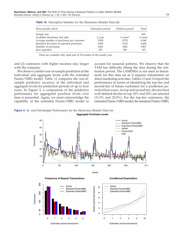
and (2) customers with higher incomes stay longerwith the company.

We observe a better out-of-sample prediction at theindividual and aggregate levels with the extendedPareto/NBD model. Table 12 compares the out-of-sample predictive accuracy at the individual andaggregate levels for prediction periods of up to fouryears. In Figure 3, a comparison of the predictiveperformance for aggregated purchase levels overtime is presented. Again, we must acknowledge thecapability of the extended Pareto/NBD model to

account for seasonal patterns. We observe that theTAM has difficulty fitting the data during the esti-mation period. The LAMDMA is not used as bench-mark for this data set as it requires information ondirect marketing activities. Tables 13 and 14 report theperformance in terms of identifying the top-tier andsecond-tier of future customers for a prediction pe-riod of four years. As top and second tier, the next bestwell-defined deciles to top 10% and 20% are selected(11.9% and 20.9%). For the top-tier customers, theextended Pareto/NBDmodel, the standard Pareto/NBD,

Table 10. Descriptive Statistics for the Electronics Retailer Data Set


Sample size — — 829Available timeframe and split 2 year 4 yearsa 6 yearsAverage number of purchases per customer 3.090 4.570 6.040Standard deviation of repeated purchases 2.980 5.023 6.406Number of purchases 2562 2445 5007Zero repeaters 276 294 129

aData are available only until end of November in the fourth year.

Figure 3. In- and Out-Sample Performance for the Electronics Retailer Data Set


and Pareto/GGG models identify 41.41% correctly.The TAM and GPPM reach 40.40%. For the pre-diction of the second-tier customers, the extendedPareto/NBD model and the standard Pareto/NBDmodel perform the same with 47.40% and slightly bet-ter compared with the Pareto/GGG model (46.24%),the TAM (43.35%), and the GPPM (45.66%). Resultsfor DECT/DERT show similar performance for thestandard and the extended Pareto/NDB model.Detailed results for DECT/DERT are reported inAppendix D. We elaborate on possible reasons forvarying degrees of performance improvements ofthe extended Pareto/NBD model in the discus-sion section.

4.3. Sporting Goods Retailer

The third data set contains transactional recordsfrom a sporting goods retailer that cover 1,071 cus-tomers who first purchased in the three-month periodbetween January andMarch 2008. In total, the data setcontains 2,226 transactions between January 2008 toDecember 2013. It is important to note that the retaileris highly specialized and sells goods for a niche sport.The key descriptive statistics are shown in Table 15.Because of the relatively large interpurchase times,the standard and extended Pareto/NBD models arefitted for a two-year estimation period. We evaluatethe predictive performance of the models for thefollowing four years.

Table 11. Parameter Estimates for the Electronics Retailer Data Set

ExtendedPareto/NBD

StandardPareto/NBD Description

LL value −7,713.724 −7,763.564BIC 15,494.651 15,554.009r 1.446*** 1.633*** Homogeneity (purchase process)α 36.771*** 40.490*** Scale parameter (purchase process)s 0.524*** 0.308*** Homogeneity (attrition process)β 12.963 · 7.238** Scale parameter (attrition)γpurch, 1 0.674*** — Seasonality (purchase process)γpurch, 2 0.021 — Gender (purchase process; male = 0, female = 1)γpurch, 3 −0.102 — Income (purchase process)γattr, 1 −0.376 — Seasonality (attrition process)γattr, 2 0.377 — Gender (attrition process; male = 0, female = 1)γattr, 3 −0.978* — Income (attrition process)

.; p < 0.1; *p < 0.05; **p < 0.01; ***p < 0.001.

Table 12. Predictive Performance for the Electronic Retailer Data Set

MetricExtended

Pareto/NBDStandard

Pareto/NBD TAM Pareto/GGG GPPM

One-year prediction IndividualMAE 0.809 0.835 0.847 0.851 0.976Correlation 0.520 0.519 0.401 0.520 0.434AggregatedMAE 3.935 5.353 12.164 5.137 7.639

Two-year prediction IndividualMAE 1.493 1.542 1.621 1.541 1.657Correlation 0.504 0.504 0.337 0.490 0.419AggregatedMAE 4.788 5.941 12.626 5.824 6.919

Three-year prediction IndividualMAE 2.118 2.200 2.353 2.142 2.286Correlation 0.491 0.493 0.287 0.481 0.406AggregatedMAE 4.573 5.545 12.895 5.807 6.381

Four-year predictiona IndividualMAE 2.522 2.659 2.791 2.564 2.783Correlation 0.468 0.471 0.248 0.461 0.378AggregatedMAE 4.635 5.482 12.738 5.768 6.150

Note. Because no direct marketing variables are available for this data set, LAMDMA results are not reported.aData are available only until end of November in the fourth year.


We include three contextual factors: (1) direct mar-keting, (2) direct marketing squared, and (3) seasonalbuying patterns. The direct marketing activities of theretailer are based on emails, which are sent out by themarketing department. The marketing activities aremeasured on a weekly basis. There is also an option toopt-out of the newsletters. To model the saturationeffects of direct marketing, we also include its squaredvalue (Schroeder and Hruschka 2016). Furthermore,an increased level of purchases is reported by thestoremanager during the Christmas season.Wemodelthis seasonal pattern by using a weekly dummy var-iable indicating high season as an aggregate-levelcontextual factor (based on expert knowledge). Thecontextual factor of direct marketing is highly likelyto be endogenous. We observe that regular customersare more often subject to marketing emails than cus-tomers who do not make frequent purchases. Therefore,we additionally estimate a variation of the extendedPareto/NBD model, where we control for the endoge-nous direct marketing contextual factors using theproposed copula correction approach.

Our results show that the extended model has abetter in-sample fit based on LL and BIC,which is alsoconfirmed by the frequency of repeat transactionsplot in Figure 4. We observe that controlling forendogeneity slightly reduces the in-sample fit. Allparameter estimates are reported in Table 16. Thecoefficients of the contextual factors suggest the fol-lowing. (1) Direct marketing activities increase thetransaction levels. However, the impact of directmarketing on customer attrition is not significant.We observe that controlling for endogeneity changesthe effect size of directmarketing. (2) Seasonal patterns

increase the transaction levels and decrease cus-tomer churn.The extended model outperforms all benchmark

models in terms of the out-of-sample prediction andthe identification of the future best customers. How-ever, likely because of the small sample size, theGPPMdid not converge after multiple trials, and thus, theresults are not reported. Table 17 compares the out-of-sample predictive accuracy of the four models at theindividual and aggregate levels. The performanceis compared for prediction periods of up to fouryears. We observe better predictive performanceacross all prediction periods. Controlling for theendogenous contextual direct marketing factor inthe estimation and the holdout period reduces thepredictive accuracy of the extended Pareto/NBDmodel. In Figure 4, the model performance for ag-gregated purchases levels in comparison with theactual levels of transactions are reported. The ex-tended Pareto/NBD model captures the increase inpurchase levels caused by seasonal patterns. Tables 18and 19 illustrate the performance in terms of identi-fying the top-tier and second-tier future customersfor a prediction period of four years. As top andsecond tier, the next best well-defined deciles to top10% and 20% are selected (11.67% and 24.18%). Weobserve that the extended Pareto/NBD model iden-tifies the best future customers more accurately. Theextended model identifies 55.77% of the second-tiercustomers correctly compared with 50.77% in thestandard model. This is a 10% improvement. A per-formance assessment based on DECT/DERT yieldsthe same results. Detailed results are reported inAppendix D.

Table 13. Predictive Performance in Identifying the Top-Tier Customers in the Electronics Retailer Data Set

Top-tier customers(four-year prediction)

ExtendedPareto/NBD

StandardPareto/NBD TAM Pareto/GGG GPPM

High, correctly classified (%) 42.41 41.41 40.40 41.41 40.40Low, correctly classified (%) 92.05 92.05 91.92 92.05 91.92Overall correctly classified (%) 86.01 86.01 85.77 86.01 85.77High, incorrectly classified (%) 7.95 7.95 8.08 7.95 8.08Low, incorrectly classified (%) 58.59 58.59 59.60 58.59 59.60Overall incorrectly classified (%) 13.99 13.99 14.24 13.99 14.23

Table 14. Predictive Performance in Identifying the Second-Tier Customers in the Electronics Retailer Data Set

Second-tier customers(four-year prediction)

ExtendedPareto/NBD

StandardPareto/NBD TAM Pareto/GGG GPPM

High, correctly classified (%) 47.40 47.40 43.35 46.24 45.66Low, correctly classified (%) 86.13 86.13 85.06 85.82 85.67Overall correctly classified (%) 78.05 78.05 76.36 77.56 77.32High, incorrectly classified (%) 13.87 13.87 14.94 14.18 14.33Low, incorrectly classified (%) 52.60 52.60 56.65 53.76 54.34Overall incorrectly classified (%) 21.95 21.95 23.64 22.44 22.68


5. DiscussionAlthough probabilistic latent customer attritionmodelsare widely used for customer base analyses, it has notbeen possible to account for time-varying contextualfactors in continuous noncontractual settings. Com-plementing the previous literature, we propose anapproach that combines the following properties:(1) the continuous nature of both the purchase and theattrition processes, (2) the inclusion of multiple time-varying and time-invariant contextual factors that canseparately influence one, both, or none of the pro-cesses, (3) gamma heterogeneity for both processes,

(4) the ability to reduce to the standard Pareto/NBDmodel when it is estimated without any contextualfactors, (5) a closed-form maximum-likelihood solu-tion, and (6) the derivation of relevant managerialexpressions. These properties have been found to beadvantageous by previous studies but have not yetbeen combined within a single modeling approach.Using three continuous, noncontractual retailing

data sets, we show that including time-invariant andtime-varying contextual factors significantly improvesthe model fit and predictive accuracy over those ofthe standard Pareto/NBD model and various other

Figure 4. In- and Out-Sample Performance for the Sporting Goods Retailer: The Extended Pareto/NBD Model with andwithout Copula Results in an Almost Identical Aggregated Curve

Table 15. Descriptive Statistics for the Sporting Goods Retailer


Sample size — — 1,071Available timeframe and split 2 years 4 years 6 yearsAverage number of purchases per customer 1.490 2.423 2.078Standard deviation of repeated purchases 0.948 2.580 2.267Number of purchases 1596 630 2226Zero repeaters 738 811 629


Pareto- and non–Pareto-type models. In particular,we observe better accuracy for individual-level pre-dictions for the first and third data set. For thesedatasets, we include time-varying contextual factorsthat affect customers not only at the aggregate level,that is, all customers in the same way, but also at theindividual level. For the second data set, we in-clude only an aggregate-level time-varying contex-tual factor. Althoughwe stillfindbetter individual-levelpredictive accuracy, the improvements are smaller thanthose of the other two data sets. To significantly improvethe individual-level prediction, additional time-varyinginformation on the individual customer is needed.

Adding time-varying contextual factors that affect thecustomers at the aggregate-level only (i.e., seasonalitypattern) mainly leads to better aggregate-level pre-dictions; however, they do not seem to have a sig-nificant effect on the individual-level predictions. Insummary, adding contextual factors enhances themanagerial applicability of the Pareto/NBD modelbecause it enables managers to better identify the bestfuture customers andpaves theway formore accurateindividual predictions for future customer purchaseand attrition behavior. Hence, fully leveraging thecapabilities of the proposedmodel requires that time-varying contextual factors be considered. Although this

Table 17. Predictive Performance for the Sporting Goods Retailer Data Set

MetricExtended

Pareto/NBDExtended

Pareto/NBD CopulaStandard

Pareto/NBD TAM Pareto/GGG LAMDMA

One-year prediction IndividualMAE 0.274 0.275 0.547 0.284 0.283 0.335Correlation 0.484 0.459 0.286 0.448 0.468 0.143AggregatedMAE 1.989 1.991 2.042 2.081 2.225 2.075

Two-year prediction IndividualMAE 0.452 0.452 0.547 0.467 0.470 0.587Correlation 0.524 0.500 0.286 0.503 0.519 0.140AggregatedMAE 1.824 1.828 1.885 2.704 2.056 2.058

Three-year prediction IndividualMAE 0.594 0.599 0.715 0.626 0.625 0.799Correlation 0.551 0.538 0.296 0.518 0.533 0.191AggregatedMAE 1.659 1.660 1.759 2.492 1.954 2.045

Four-year prediction IndividualMAE 0.741 0.759 0.843 0.787 0.779 1.010Correlation 0.551 0.536 0.297 0.518 0.532 0.198AggregatedMAE 1.610 1.624 1.698 2.412 1.877 2.048

Note. The GPPM did not converge; results are not reported.

Table 16. Parameter Estimates for the Sporting Goods Retailer Data Set

Extended Pareto/NBD Extended Pareto/NBD Copula Standard Pareto/NBD Description

LL value −3,107.808 −3,112.204 −3,212.551BIC 6,285.379 6,322.077 6,453.008r 1.838*** 1.583*** 1.412** Homogeneity (purchase process)α 179.429** 177.629*** 163.862*** Scale parameter (purchase process)s 0.451** 0.442** 0.270** Homogeneity (attrition process)β 29.203* 23.484* 5.784* Scale parameter (attrition)γpurch, 1 1.950*** 1.911*** — Direct marketing (purchase process)

γpurch, 2 0.406*** 0.336* — (Direct marketing)2 (purchase process)γpurch, 3 0.747*** 0.755*** — Seasonality (purchase process)γpurch, 4 — 0.010 — Copula correction term DM (purchase process)γpurch, 5 — 0.004 — Copula correction term DM2 (purchase process)γattr, 1 0.064 0.157 — Direct marketing (attrition process)γattr, 2 2.591 2.251 — (Direct marketing)2 (attrition process)γattr, 3 −0.101** −0.091** — Seasonality (attrition process)γattr, 4 — −0.013 — Copula correction term DM (attrition process)γattr, 5 — −0.222 — Copula correction term DM2 (attrition process)

*p < 0.05; **p < 0.01; ***p < 0.001.


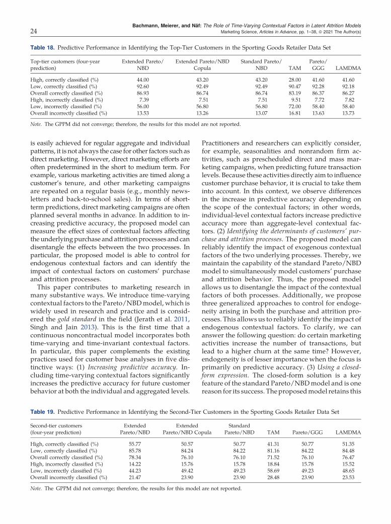
is easily achieved for regular aggregate and individualpatterns, it is not always the case for other factors such asdirect marketing. However, direct marketing efforts areoften predetermined in the short to medium term. Forexample, various marketing activities are timed along acustomer’s tenure, and other marketing campaignsare repeated on a regular basis (e.g., monthly news-letters and back-to-school sales). In terms of short-term predictions, direct marketing campaigns are oftenplanned several months in advance. In addition to in-creasing predictive accuracy, the proposed model canmeasure the effect sizes of contextual factors affectingthe underlyingpurchase and attritionprocesses and candisentangle the effects between the two processes. Inparticular, the proposed model is able to control forendogenous contextual factors and can identify theimpact of contextual factors on customers’ purchaseand attrition processes.

This paper contributes to marketing research inmany substantive ways. We introduce time-varyingcontextual factors to the Pareto/NBDmodel, which iswidely used in research and practice and is consid-ered the gold standard in the field (Jerath et al. 2011,Singh and Jain 2013). This is the first time that acontinuous noncontractual model incorporates bothtime-varying and time-invariant contextual factors.In particular, this paper complements the existingpractices used for customer base analyses in five dis-tinctive ways: (1) Increasing predictive accuracy. In-cluding time-varying contextual factors significantlyincreases the predictive accuracy for future customerbehavior at both the individual and aggregated levels.

Practitioners and researchers can explicitly consider,for example, seasonalities and nonrandom firm ac-tivities, such as prescheduled direct and mass mar-keting campaigns, when predicting future transactionlevels. Because these activities directly aim to influencecustomer purchase behavior, it is crucial to take theminto account. In this context, we observe differencesin the increase in predictive accuracy depending onthe scope of the contextual factors; in other words,individual-level contextual factors increase predictiveaccuracy more than aggregate-level contextual fac-tors. (2) Identifying the determinants of customers’ pur-chase and attrition processes. The proposed model canreliably identify the impact of exogenous contextualfactors of the two underlying processes. Thereby, wemaintain the capability of the standard Pareto/NBDmodel to simultaneously model customers’ purchaseand attrition behavior. Thus, the proposed modelallows us to disentangle the impact of the contextualfactors of both processes. Additionally, we proposethree generalized approaches to control for endoge-neity arising in both the purchase and attrition pro-cesses. This allows us to reliably identify the impact ofendogenous contextual factors. To clarify, we cananswer the following question: do certain marketingactivities increase the number of transactions, butlead to a higher churn at the same time? However,endogeneity is of lesser importance when the focus isprimarily on predictive accuracy. (3) Using a closed-form expression. The closed-form solution is a keyfeature of the standard Pareto/NBDmodel and is onereason for its success. The proposedmodel retains this

Table 18. Predictive Performance in Identifying the Top-Tier Customers in the Sporting Goods Retailer Data Set

Top-tier customers (four-yearprediction)

Extended Pareto/NBD

Extended Pareto/NBDCopula

Standard Pareto/NBD TAM

Pareto/GGG LAMDMA


Note. The GPPM did not converge; therefore, the results for this model are not reported.

Table 19. Predictive Performance in Identifying the Second-Tier Customers in the Sporting Goods Retailer Data Set

Second-tier customers(four-year prediction)

ExtendedPareto/NBD

ExtendedPareto/NBD Copula

StandardPareto/NBD TAM Pareto/GGG LAMDMA


Note. The GPPM did not converge; therefore, the results for this model are not reported.


key feature. The closed-form solution allows us toderive additional expressions such as P(alive) and theconditional expectation for any customer. These ex-pressions allow researchers and practitioners to gainan intuitive understanding of the predicted customerbehavior. Additionally, a closed-form solution allowsfor robust, scalable, and efficient implementation.Although the computational resources needed forcalculations have increased significantly during thelast few years, in an ever-increasing competitiveenvironment, efficient implementation is still key formarketers to gain access to relevant and reliable in-formation in a timely manner. (4) Scenario analysis. Byproposing an approach that involves an efficientmodel that controls for endogenous contextual fac-tors, we have taken the first step toward enablingpractitioners to perform scenario analyses (Hruschka2010). Given that many contextual factors can bedirectly influenced by the company itself, a scenarioanalysis might help practitioners make the right de-cisions. For example, in the case of direct marketingactivities, managers, who have access to informationon the cost of specific actions and are bound to budgetrestrictions, could assess a hypothetical sequence ofvarious personalized marketing campaigns to de-termine which one is most efficient in improving ei-ther the lifetime value of an individual customer orthe firm’s customer equity. (5) DECT. To ensure themanagerial relevance of modeling customer latentattrition, we propose, similar to Fader et al. (2005b), acorresponding metric. The proposed DECT metricmeasures the flow of future transactions discountedto the present value, which is important for mana-gerial applications. Furthermore, managers can as-sess individual customer valuations by using theDECTmetric in combination with a Gamma/Gammamodel for modeling customer spending.

Finally, we identified five limitations that can beaddressed by future research efforts in this field. First,the impact of tactical marketing activities is usuallynot restricted to the customer purchase and attritionprocesses. These marketing activities likely influencecustomer spending. Neither the Pareto/NBD model

nor our extension accounts for the spending processof customers. Further research could focus on mod-eling the impact of contextual factors on the spendingprocess. Second, a study may leverage the extendedPareto/NBD model to gain further insights on theimportance of clumpiness (Zhang et al. 2015) or dif-ferences in the interpurchase times of customers (Platzerand Reutterer 2016). Platzer and Reutterer (2016)showed that patterns of interpurchase times mayprovide additional insights for the prediction of fu-ture customer behavior. However, their model doesnot account for any contextual factors other than fixedregularity patterns. Future research may combine thecapabilities of the extended Pareto/NBD and thePareto/GGG model. Third, future research may an-alyze the individual responsiveness of customers tocontextual factors. The proposed extended Pareto/NBDmodel assumes that all customers have the samedegree of responsiveness. A fourth promising direc-tion for future research is to model common patternsacross cohorts. Most studies on probabilistic cus-tomer attrition models, including this one, assumethat the cohorts are independent of each other. Al-though it is possible to use a pooled model and toaccount for cohort-specific differences by includingfixed effects in the extended Pareto/NBD model, thisis not an optimal solution. Leveraging the common-alities between cohorts, similar to the cross-cohortmodel introduced by Gopalakrishnan et al. (2017),could possibly improve the predictions, especially forcohorts that have been observed for only a relativelyshort period of time. Fifth, future research may addfurther benchmarks. Although we provide a com-parison with a wide set of benchmark models, thereexist further approaches that the proposed extendedPareto/NBD model can be compared with (e.g., thehiddenMarkowmodel proposed byNetzer et al. 2008or the approach proposed by Allenby et al. 1999).Finally, on a different note, the computational aspectsof the extended Pareto/NBD model deserve furtherattention. The complexity of the extended Pareto/NBD model increases computational requirements.See Table 20 for a run time comparison of all benchmark

Table 20. Run Time Comparison

Model Timing Implementation

With time-varying contextualfactors

Extended Pareto/NBD

6 h, 51min CLVTools (Bachmann et al.2020)

Transaction attribute 8 h, 10 min OwnGPPM 9 h, 57min Dew and Ansari (2018)LAMDMA 5 h, 48min Own

No time-varying contextual factors Standard Pareto/NBD

<1 min CLVTools (Bachmann et al.2020)

Pareto/GGG 8 min BTYDplus (Platzer 2018)

Note. Detailed specifications for the run time comparison are provided in Appendix E.


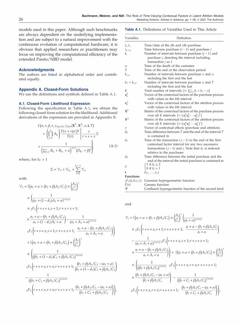
models used in this paper. Although such benchmarksare always dependent on the underlying implementa-tion and are subject to a natural improvement with thecontinuous evolution of computational hardware, it isobvious that applied researchers or practitioners mayfocus on improving the computational efficiency of theextended Pareto/NBD model.

AcknowledgmentsThe authors are listed in alphabetical order and contrib-uted equally.

Appendix A. Closed-Form SolutionsWe use the definitions and symbols defined in Table A.1.

A.1. Closed-Form Likelihood Expression

Following the specification in Table A.1, we obtain thefollowing closed-form solution for the likelihood.Additionalderivations of the expression are provided in Appendix B.


( )

∏x

j1

Akj

( )Γ x + r( )αrβs

Γ r( )

s

r + s + xZ

[

+1

∑xj1 Bkj + BkT + α

( )x+rDkT + β( )s

⎤⎥⎥⎥⎥⎥⎥⎥⎥⎥⎥⎥⎥⎥⎥⎥⎥⎥⎥⎥⎥⎥⎥⎥⎦, (A.1)

where, for kT > 1

Z Y1 + YkT +∑kT−1

i2

Yi,

with

Y1 I a1 +α > b1 + β( )

A1/C1

×

A1

C1

( )s

×1

a1 + 1− d1( )A1 +α( )r+s+x

(

× 2F1 r+ s+ x, s+ 1; r+ s+ x+ 1;

(

×a1 +α− b1 + β

( )A1/C1

a1 + 1− d1( )A1 +α

)−

1

a1 +A1 +α( )r+s+x

2F1 r+ s+ x, s+ 1; r+ s+ x+ 1;

(a1 +α− b1 + β

( )A1/C1

a1 +A1 +α

))

+ I a1 +α < b1 + β( )

A1/C1

×

A1

C1

( )s

×1

b1 + 1− d1( )C1 + β( )

A1/C1

( )r+s+x

(

2F1 r+ s+ x, r+ x; r+ s+ x+ 1;

(b1 + β( )

A1/C1 − a1 +α( )

b1 + 1− d1( )C1 + β( )

A1/C1

)

−1

b1 +C1 + β( )

A1/C1

( )r+s+x .

2F1 r+ s+ x, r+ x; r+ s+ x+ 1;b1 + β( )

A1/C1 − a1 +α( )

b1 +C1 + β( )

A1/C1

( ))

,

and

Yi I ai +α > bi + β( )

Ai/Ci

×

Ai

Ci

( )s 1

ai +α( )r+s+x

(

× 2F1

(

r+ s+ x, s+ 1; r+ s+ x+ 1;ai +α− bi + β

( )Ai/Ci

ai +α

)

−1

ai +Ai +α( )r+s+x2F1 r+ s+ x, s+ 1; r+ s+ x+ 1;

(

×ai +α− bi + β

( )Ai/Ci

ai +Ai +α

))

+ I ai +α < bi + β( )

Ai/Ci

×

Ai

Ci

( )s

×1

bi + β( )

Ai/Ci

( )r+s+x

(

2F1 r+ s+ x, r+ x; r+ s+ x+ 1;

(

×bi + β( )

Ai/Ci − ai +α( )

bi + β( )

Ai/Ci

)

−1

bi +Ci + β( )

Ai/Ci

( )r+s+x

2F1 r+ s+ x, r+ x; r+ s+ x+ 1;

(bi + β( )

Ai/Ci − ai +α( )

bi +Ci + β( )

Ai/Ci

))

,

Table A.1. Definitions of Variables Used in This Article

Variables Definition

tj, tx Time/date of the jth and xth purchasezj−1,j Time between purchase (j − 1) and purchase jkj Number of intervals between purchase (j − 1) and

purchase j, denoting the interval includingtransaction j as 1

ω Time of the death of the customerT Time of the end of the observation periodkx,ω Number of intervals between purchase x and ω

including the first and the lastkT kx,T Number of intervals between purchase x and T

including the first and the lastK Total number of intervals: [

∑xj1 kj + kT − x]

xPk Vector of the contextual factors of the purchase processwith values in the kth interval

xAk Vector of the contextual factors of the attrition processwith values in the kth interval

XP Matrix of the contextual factors of the purchase processover all K intervals: [ xP1x

P2 · · · x

PK

( )′]

XA Matrix of the contextual factors of the attrition processover all K intervals: [ xA1 x

A2 · · · xAK

( )′]

γ Vector of contextual effects (purchase and attrition).dT Time difference between T and the end of the interval T

is contained ind1 Time of the transaction ( j − 1) to the end of the first

contextual factor interval for any two successivetransactions ( j − 1) and j. Note that d1 is indexedrelative to the purchases

d2 Time difference between the initial purchase and theend of the interval the initial purchase is contained in

δ1 if kj ≥ 20 if kj 1

t (t1, . . . , tx)Functions

2F1(a, b; c; z) Gaussian hypergeometric functionΓ(x) Gamma functionΨ Confluent hypergeometric function of the second kind


for i 2, . . . , k − 1 and

YkT I akT + α > bkT + β( )

AkT/CkT

×

AkT

CkT

( )s

×1

akT + α( )r+s+x

(

2F1 r + s + x, s + 1; r + s + x + 1;

(

akT + α − bkT + β( )

AkT/CkT

akT + α

)

−1

a∗T + α( )r+s+x

2F1 r + s + x, s + 1; r + s + x + 1;

(

akT + α − bkT + β( )

AkT/CkT

a∗T + α

))

+ I akT + α < bkT + β( )

AkT/CkT

×

AkT

CkT

( )s

×1

bkT + β( )

AkT/CkT

( )r+s+x

(

2F1 r + s + x, r + x; r + s + x + 1;

(

bkT + β( )

AkT/CkT − akT + α( )

bkT + β( )

AkT/CkT

)

−1

b∗T + β( )

AkT/CkT

( )r+s+x

2F1 r + s + x, r + x; r + s + x + 1;

(

bkT + β( )

AkT/CkT − akT + α( )

b∗T + β( )

AkT/CkT

))

.

While for kT 1,

Z I a1 + α > b1 + β( )

A1/C1

×

A1

C1

( )s

×1

a1 + 1 − d1( )A1 + α( )r+s+x

(

2F1 r + s + x, s + 1; r + s + x + 1;

(a1 + α − b1 + β

( )A1/C1

a1 + 1 − d1( )A1 + α

)

−1

aT1 + α( )r+s+x 2F1 r + s + x, s + 1; r + s + x + 1;

(

a1 + α − b1 + β( )

A1/C1

aT1 + α

))

+ I a1 + α < b1 + β( )

A1/C1

×

A1

C1

( )s

×1

b1 + 1 − d1( )C1 + β( )

A1/C1

( )r+s+x

(

2F1

(

r + s + x, r + x; r + s + x + 1; .

b1 + β( )

A1/C1 − a1 + α( )

b1 + 1 − d1( )C1 + β( )

A1/C1

)

−1

bT1 + β( )

A1/C1

( )r+s+x

2F1

(

r + s + x, s + 1; r + s + x + 1; .

b1 + β( )

A1/C1 − a1 + α( )

bT1 + β( )

A1/C1

))

,

with i 1, . . . , kT ,

Akj exp γ′purchx

Pkj

( ),

Bkj exp γ′purchx

P1

( )d1 +

∑kj−1

l2

exp γ′purchx

Pl

( )

+ exp γ′purchx

Pkj

( )zj−1,j − d1 − δ kj − 2

( )[ ],

Ai exp γ′purchx

Pi

( ),

Ci exp γ′attrx

Ai

( ),

Bi exp γ′purchx

P1

( )d1 +

∑i−1

l2

exp γpurchxPl

( )

+ exp γ′purchx

Pi

( )−tx − d1 − I i ≥ 2 i − 2( )[ ],

Di exp γ′attrx

A1

( )d2 +

∑k0,x+i−2

l2

exp γ′attrx

Al

( )+

+ exp γ′attrx

Ak0,x+i−1

( )−d2 − I k0,x + i − 1 ≥ 2

[

× k0,x + i − 3( )],

DkT exp γ′attrx

Ak0,x+kT−1

( )T + DkT ,

ai ∑x

j1

Bkj + Bi + tx + d1 + i − 2( )( )Ai,

bi Di + tx + d1 + i − 2( )( )Ci,

a∗T ∑x

j1

Bkj + BkT + TAkT ,

b∗T DkT + TCkT ,

aT1 ∑x

j1

Bkj + B1 + TA1,

bT1 D1 + TC1.

A.2. P(alive)

Following the specifications in Table A.1 and Appendix A.1,we obtain the following closed-form solution for P(alive):

P Ω > T|r, α, s, β, γpurch, γattr,XP,XA, x, tx,T

( )

∏x

j1

Akj

Γ x + r( )αrβs

Γ r( )∑x

j1 Bkj + BkT + α( )x+r

DkT + β( )s

×1


( )

∫∞

0

∫∞

0

∏x

j1

λ0Akj exp −λ0Bkj

[ ][ ]

exp −λ0BkT

[ ]

× exp −μ0DkT

[ ]g λ0( )g μ0

( )dλ0dμ0

×1


( )

1


( )x+rDkT + β( )s s

r+s+xZ + 1. (A.2)


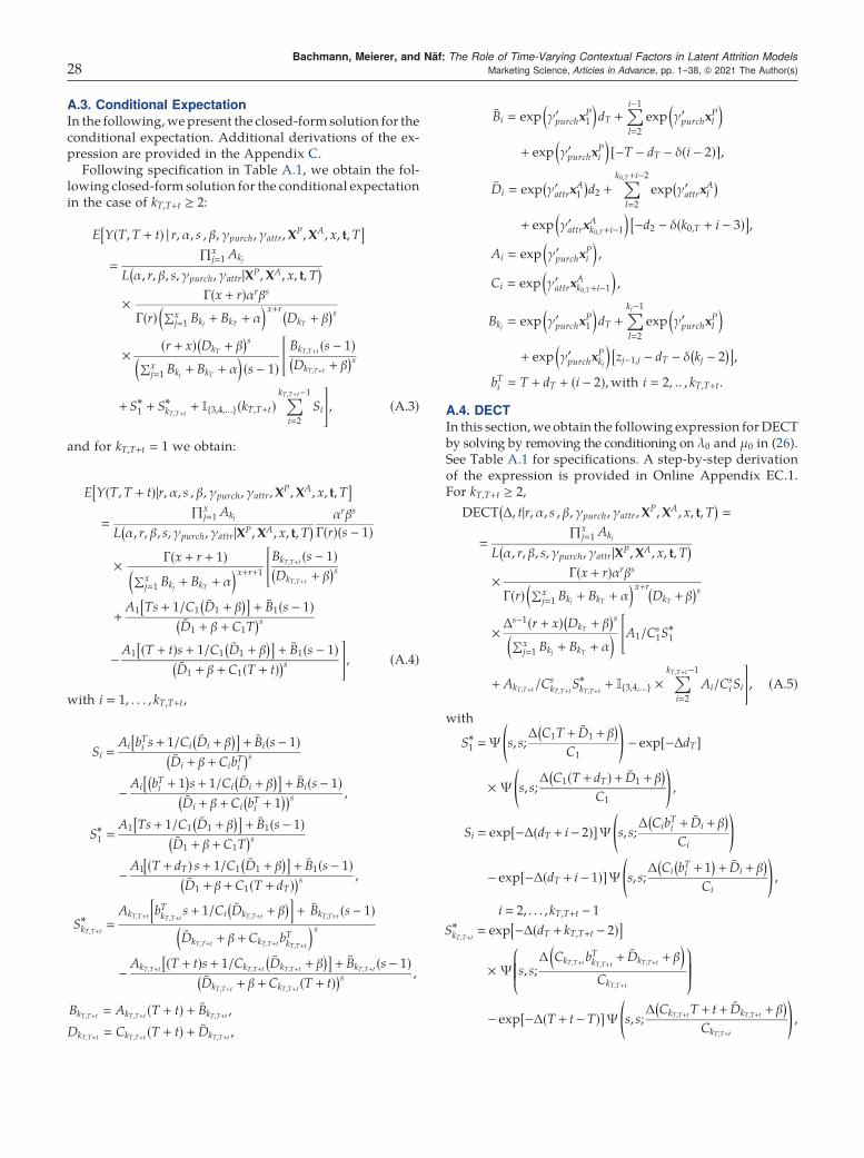
A.3. Conditional Expectation

In the following,we present the closed-form solution for theconditional expectation. Additional derivations of the ex-pression are provided in the Appendix C.

Following specification in Table A.1, we obtain the fol-lowing closed-form solution for the conditional expectationin the case of kT,T+t ≥ 2:

E Y T,T + t( ) | r, α, s , β, γpurch, γattr,XP,XA, x, t,T

[ ]

∏xj1 Akj


( )

×Γ x + r( )αrβs

Γ r( )∑x


DkT + β( )s

×r + x( ) DkT + β

( )s


( )s − 1( )

BkT,T+t s − 1( )

DkT,T+t + β( )s

[

+S∗1 + S∗kT,T+t + I 3,4,... kT,T+t( )∑kT,T+t−1

i2

Si

]

, (A.3)

and for kT,T+t 1 we obtain:

E Y T,T + t( )|r, α, s , β, γpurch, γattr,XP,XA, x, t,T

[ ]

∏xj1 Akj


( ) αrβs

Γ r( ) s − 1( )

×Γ x + r + 1( )


( )x+r+1BkT,T+t s − 1( )

DkT,T+t + β( )s

[

+A1 Ts + 1/C1 D1 + β

( )[ ]+ B1 s − 1( )

D1 + β + C1T( )s

−A1 T + t( )s + 1/C1 D1 + β

( )[ ]+ B1 s − 1( )

D1 + β + C1 T + t( )( )s

]

, (A.4)

with i 1, . . . , kT,T+t,

Si Ai b

Ti s + 1/Ci Di + β

( )[ ]+ Bi s − 1( )

Di + β+ CibTi( )s

−Ai bTi + 1

( )s+ 1/Ci Di + β

( )[ ]+ Bi s − 1( )

Di + β+ Ci bTi + 1( )( )s ,

S∗1 A1 Ts+ 1/C1 D1 + β

( )[ ]+ B1 s− 1( )

D1 + β+ C1T( )s

−A1 T + dT( ) s + 1/C1 D1 + β

( )[ ]+ B1(s− 1)

D1 + β + C1 T + dT( )( )s ,

S∗kT,T+t AkT,T+t b

TkT,T+t

s+ 1/Ci DkT,T+t + β( )[ ]

+ BkT,T+t s− 1( )

DkT,T+t + β + CkT,T+tbTkT,T+t

( )s

−AkT,T+t T + t( )s + 1/CkT,T+t DkT,T+t + β

( )[ ]+ BkT,T+t s− 1( )

DkT,T+t + β+ CkT,T+t T + t( )( )s ,

BkT,T+t AkT,T+t T + t( ) + BkT,T+t ,

DkT,T+t CkT,T+t T + t( ) + DkT,T+t ,

Bi exp γ′purchx

P1

( )dT +

∑i−1

l2

exp γ′purchx

Pl

( )

+ exp γ′purchx

Pi

( )−T − dT − δ i − 2( )[ ],

Di exp γ′attrx

A1

( )d2 +

∑k0,T+i−2

l2

exp γ′attrx

Al

( )

+ exp γ′attrx

Ak0,T+i−1

( )−d2 − δ k0,T + i − 3( )[ ]

,

Ai exp γ′purchx

Pi

( ),

Ci exp γ′attrx

Ak0,T+i−1

( ),

Bkj exp γ′purchx

P1

( )dT +

∑kj−1

l2

exp γ′purchx

Pl

( )

+ exp γ′purchx

Pkj

( )zj−1,j − dT − δ kj − 2

( )[ ],

bTi T + dT + i − 2( ),with i 2, .. , kT,T+t.

A.4. DECT

In this section,we obtain the following expression forDECTby solving by removing the conditioning on λ0 and μ0 in (26).See Table A.1 for specifications. A step-by-step derivationof the expression is provided in Online Appendix EC.1.For kT,T+t ≥ 2,

DECT ∆, t|r, α, s , β, γpurch, γattr,XP,XA, x, t,T

( )

∏xj1 Akj


( )

×Γ x + r( )αrβs

Γ r( )∑x


DkT + β( )s

×∆s−1 r + x( ) DkT + β

( )s


( ) A1/Cs1S∗1

[

+ AkT,T+t/CskT,T+t

S∗kT,T+t + I 3,4,... ×∑kT,T+t−1

i2

Ai/CsiSi

]

, (A.5)

with

S∗1 Ψ s, s;∆ C1T + D1 + β( )

C1

( )

− exp −∆dT[ ]

× Ψ s, s;∆ C1 T + dT( ) + D1 + β( )

C1

( )

,

Si exp −∆ dT + i− 2( )[ ]Ψ s, s;∆ Cib

Ti + Di + β

( )

Ci

( )

− exp −∆ dT + i− 1( )[ ]Ψ s, s;∆ Ci b

Ti + 1

( )+ Di + β

( )

Ci

( )

,

i 2, . . . , kT,T+t − 1

S∗kT,T+t exp −∆ dT + kT,T+t − 2( )[ ]

× Ψ s, s;∆ CkT,T+tb

TkT,T+t

+ DkT,T+t + β( )

CkT,T+t

⎛⎜⎜⎜⎜⎜⎜⎜⎜⎜⎜⎜⎝

⎞⎟⎟⎟⎟⎟⎟⎟⎟⎟⎟⎟⎠

− exp −∆ T + t−T( )[ ]Ψ s, s;∆ CkT,T+tT + t+ DkT,T+t + β( )

CkT,T+t

( )

,


DkT,t CkT,t t + DkT,t ,

Di exp γ′attrx

A1

( )d2 +

∑k0,T+i−2

l2

exp γ′attrx

Al

( )

+ exp γ′attrx

Ak0,T+i−1

( )−d2 − δ k0,T + i − 3( )[ ]

,

DkT DkT,0 CkTT + DkT ,

Ai exp γ′purchx

Pi

( ), i 1, . . . , kT,T+t

Ci exp γ′purchx

Ak0,T+i−1

( ),

bTi T + dT + i − 2( ), i 2, .. , kT,T+t

Ψ : is the confluent hypergeometric function

of the second kind.

A.5. Unconditional Expectation E[Y (t)]

In the following,we present the closed-form solution for theunconditional expectation of the number of transactions inthe interval (0, t], E[Y(t)], which is used for for the incre-mental tracking plots (Figures 2–4) to asses the aggregatedperformance of the model. We obtain the following numberof transactions in k0t 1:

E Y t( )|r, α, s , β, γpurch, γattr,XP,XA

[ ]

βsr

s − 1( )α

A1t s − 1( )

β + C1t( )s +

A1/C1

βs−1

[

−A1 ts + 1/C1β

( )

β + C1t( )s

]

,

and for k0t ≥ 2,

E Y t( )|r, α, s , β, γpurch, γattr,XP,XA

[ ]

βsr

s − 1( )α

Bk0,t s − 1( )

β +Dk0,t

( )s + S∗1 + S∗k0,t +∑k0,t−1

i2

Si

[ ]

,

where

Si Ai b

0i s + 1/Ci β + Di

( )[ ]+ Bi s − 1( )

β + Di + Cib0i

( )s

−Ai b0i + 1

( )s + 1/Ci β + Di

( )[ ]+ Bi s − 1( )

β + Di + Ci b0i + 1

( )( )s ,

S∗1 A1/C1 β + D1

( )+ B1 s − 1( )

β + D1

( )s

−A1 d1s + 1/C1 β + D1

( )[ ]+ B1 s − 1( )

β + D1 + C1d1( )s ,

S∗k0,t Ak0,t b

0k0,ts + 1/Ck0,t β + Dk0,t

( )[ ]+ Bk0,t s − 1( )

β + Dk0,t + Ck0,tb0k0,t

( )s

−Ak0,t ts + 1/Ck0,t β + Dk0,t

( )[ ]+ Bk0,t s − 1( )

β + Dk0,t + Ck0,t t( )s ,

Bk0,t Ak0,t t + Bk0,t ,

Dk0,t Ck0,t t + Dk0,t ,

Bi exp γ′purchX

P1

( )d1 +

∑i−1

l2

exp γ′purchX

Pl

( )

+ exp γ′purchX

Pi

( )−d1 − I i ≥ 2 i − 2( )[ ], i 1, . . . , k0,t

Di exp γ′attrX

A1

( )d2 +

∑i−1

l2

exp γ′attrX

Al

( )+ exp

× γ′attrX

Ai

( )−d2 − I i ≥ 2 i − 2( )[ ] , i 1, . . . , k0,t

b0i d1 + i − 2( ), i 2, .. , k0,t.

A.6. Probability Mass Function P[Y([u, t + u])) x]

In the following,we present the closed-form solution for theprobability mass function. Additional derivations of theexpression are provided in Online Appendix EC.2.

We obtain the following expression for the probabilityof the number of purchases in a given time interval [u, u + t].The expressionP(Y((u, t + u]) x|r, α, s, β, γpurch, γattr,X

P,XA)

is used for the in-sample histograms in Figures 2–4.

P X u,t+u( ]( )( x|r,α,s,β,γpurch,γattr,XP,XA

)

S1+Γ s+1( )Γ r+x( )

Γ r+s+x+1( )

∑x

j0

S21,j+S2ku,t+u ,j+∑ku,t+u−1

i2

S2i,j

( )

,

(A.6)

with

S1 Bxku,t+u

x!

Γ x + r( )

Γ r( )

αrβs

Bku,t+u + α( )x+r Dku,t+u + β

( )s ,

S2i,j I Bi + α > Di + β( )

Ai/Ci

× B

ji

1

j!

∑x−j

n0

1

n!

×As+n

i

Csi

Γ r + s + j + n( )

Γ r( )Γ s( )

bui[ ]nαrβs

Bi + Aibui + α

( )r+s+j+n

[

× 2F1 s + r + j + n, s + 1; r + s + x + 1;

(

Bi + α − Di + β( )

Ai/Ci

Bi + Aibui + α

)−

bui + 1[ ]nαrβs

Bi + Ai bui + 1( )

+ α( )r+s+j+n

× 2F1 s + r + j + n, s + 1; r + s + x + 1;

(

Bi + α − Di + β( )

Ai/Ci

Bi + Ai bui + 1( )

+ α

)]

+ I Bi + α < Di + β( )

Ai/Ci

× B

ji

1

j!

∑x−j

n0

1

n!

×Γ r + s + j + n( )

Γ r( )Γ s( )

As+ni

Csi

bui[ ]nαrβs

Di + Cibui + β

( )Ai/Ci

( )r+s+j+n

[

2F1 s + r + j + n, r + x; r + s + x + 1;

(

Di + β( )

Ai/Ci − Bi + α( )

Di + Cibui + β( )

Ai/Ci

)

−bui + 1[ ]nαrβs

Di + Ci bui + 1

( )+ β

( )Ai/Ci

( )r+s+j+n

2F1 s + r + j + n, r + x; r + s + x + 1;

(

Di + β( )

Ai/Ci − Bi + α( )

Di + Ci bui + 1( )

+ β( )

Ai/Ci

)]


S21,j I B1 + α > D1 + β( )

A1/C1

× Bj1

1

j!

∑x−j

n0

1

n!

As+n1

Cs1

Γ r + s + j + n( )

Γ r( )Γ s( )

unαrβs

B1 + A1u + α( )r+s+j+n

[

2F1 s + r + j + n, s + 1; r + s + x + 1;

(

B1 + α − D1 + β( )

A1/C1

B1 + A1u + α

)−

bu2[ ]nαrβs

B1 + A1bu2 + α( )r+s+j+n

2F1 s + r + j + n, s + 1; r + s + x + 1;

(

B1 + α − D1 + β( )

A1/C1

B1 + A1bu2 + α

)]

+ I B1 + α < D1 + β( )

A1/C1

× Bj1

1

j!

∑x−j

n0

1

n!

Γ r + s + j + n( )

Γ r( )Γ s( )

As+n1

Cs1

unαrβs

D1 + C1u + β( )

A1/C1

( )r+s+j+n

[

2F1 s + r + j + n, r + x; r + s + x + 1;

(

D1 + β( )

A1/C1 − B1 + α( )

D1 + C1u + β( )

A1/C1

)

−bu2[ ]nαrβs

D1 + C1bu2 + β( )

A1/C1

( )r+s+j+n

2F1 s + r + j + n, r + x; r + s + x + 1;

(

D1 + β( )

A1/C1 − B1 + α( )

D1 + C1bu2 + β( )

A1/C1

)

,

S2ku,t+u ,j I Bku,t+u + α > Dku,t+u + β( )

Aku,t+u/Cku,t+u

× Bjku,t+u

1

j!

∑x−j

n0

1

n!

As+nku,t+u

Csku,t+u

Γ r + s + j + n( )

Γ r( )Γ s( )

buku,t+u

[ ]nαrβs

Bku,t+u + Aku,t+ubuku,t+u

+ α( )r+s+j+n

⎡⎢⎢⎢⎢⎢⎢⎢⎢⎢⎢⎢⎢⎢⎢⎢⎢⎢⎢⎢⎢⎢⎢⎢⎢⎢⎣

2F1 s + r + j + n, s + 1; r + s + x + 1;

(

Bku,t+u + α − Dku,t+u + β( )

Aku,t+u/Cku,t+u

Bku,t+u + Aku,t+ubuku,t+u

+ α

)

−u + t[ ]nαrβs

Bku,t+u + Aku,t+u u + t( ) + α( )r+s+j+n

2F1 s + r + j + n, s + 1; r + s + x + 1;

(

Bku,t+u + α − Dku,t+u + β( )

Aku,t+u/Cku,t+u

Bku,t+u + Aku,t+u u + t( ) + α

)⎤⎥⎥⎥⎥⎥⎥⎥⎥⎥⎥⎥⎥⎥⎥⎥⎥⎥⎥⎥⎥⎥⎥⎥⎥⎥⎦

+ I Bku,t+u + α < Dku,t+u + β( )

Aku,t+u/Cku,t+u

× Bjku,t+u

1

j!

∑x−j

n0

1

n!

Γ r + s + j + n( )

Γ r( )Γ s( )

As+nku,t+u

Csku,t+u

buku,t+u

[ ]nαrβs

Dku,t+u + Cku,t+ubuku,t+u

+ β( )(

Aku,t+u/Cku,t+u

)r+s+j+n

⎡⎢⎢⎢⎢⎢⎢⎢⎢⎢⎢⎢⎢⎢⎢⎢⎢⎢⎢⎢⎢⎢⎢⎢⎢⎢⎢⎣

2F1 s + r + j + n, r + x; r + s + x + 1;

⎛⎜⎜⎜⎜⎜⎜⎜⎜⎜⎜⎜⎜⎝

Dku,t+u + β( )

Aku,t+u/Cku,t+u − Bku,t+u + α( )

Dku,t+u + Cku,t+ubuku,t+u

+ β( )

Aku,t+u/Cku,t+u

⎞⎟⎟⎟⎟⎟⎟⎟⎟⎟⎟⎟⎟⎠

−u + t[ ]nαrβs

Dku,t+u + Cku,t+u u + t( ) + β( )(

Aku,t+u/Cku,t+u

)r+s+j+n

2F1 s + r + j + n, r + x; r + s + x + 1;

(

Dku,t+u + β( )

Aku,t+u/Cku,t+u − Bku,t+u + α( )

Dku,t+u + Cku,t+u u + t( ) + β( )

Aku,t+u/Cku,t+u

)⎤⎥⎥⎥⎥⎥⎥⎥⎥⎥⎥⎥⎥⎥⎥⎥⎥⎥⎥⎥⎥⎥⎥⎥⎥⎥⎥⎦,

for i 1, . . . , ku,t+u,

Ai exp γ′purchX

Pi

( ),

Ci exp γ′attrX

Ak0,u+i−1

( ),

Bku,t+u Aku,t+u t + u( ) + Bku,t+u ,

Dku,t+u Cku,t+u t + Du,t+u,

Bi exp γ′purchX

P1

( )d1 +

∑i−1

l2

exp γ′purchX

Pl

( )

+ exp γ′purchX

Pi

( )−u − d1 − I i ≥ 2 i − 2( )[ ],

Di exp γ′attrX

A1

( )d2 +

∑k0,u+i−2

l2

exp γ′attrX

Al

( )

+ exp γ′attrX

Ak0,u+i−1

( )−d2 − I k0,u + i ≥ 3

[k0,u + i − 3( )

],

and for i 2, . . . , ku,t+u,

bui u + d1 + i − 2.

Appendix B. Additional Derivations for the

Likelihood ExpressionIn this section, we show the detailed stop for deriving theclosed-form likelihood expression. We start by distinguishingtwo cases that affect the purchase process:

Case 1. The customer is still alive at the end of the esti-mation period T. Let t (t1, . . . , tx)

′ denote the vector oftransaction times and zx,T be the time between the lasttransaction of a customer and the end of the estimation period.The probability that the lifetime of a customer is larger than T,that is, with Zx,x+1 as a random variable for the time between xand x + 1, is

P Zx,x+1 > zx,T |t( ) SP zx,T |t( ) exp −θPtxzx,T( )

[ ]. (B.1)


Then, the individual likelihood is the product of the densityfor the interpurchase time and the corresponding survivorfunction is

L λ0, γpurch|t,T,XP, x,Ω > T

( )

f P z0,1( ) ·∏x

j2

f P zj−1,j|z0,1, . . . , zj−2,j−1( )

[ ]

SP zx,T |t( )

∏x

j1


[ ][ ]

exp −λ0BkT

[ ], (B.2)

with

Akj exp γ′purchx

Pkj

( ),

Bkj exp γ′purchx

P1

( )d1 +

∑kj−1

l1

exp γ′purchx

Pl

( )[ ]

+ exp γ′purchx

Pkj

( )zj−1,j − d1 − δ kj − 2

( )[ ].

With kT as the number of intervals between the last trans-action and the end of the estimation period plus 1 and withthe discretized version of θtx (zx,T),

BkT exp γ′purchx

P1

( )d1 +

∑kj−1

l1

exp γ′purchx

Pl

( )[ ]

+ exp γ′purchx

PkT

( )T − tx( ) − d1 − δ kT − 2( )[ ].

Case 2. The customer becomes inactive between the lasttransaction and T. This means that the customer’s lifetimeends somewhere before the end of the estimation period(i.e., ω ∈ (tx,T]). Therefore, we need the probability for somefixed ω ∈ (tx,T]:

P Zx,x+1 > zx,ω|t( ) SP zx,ω|t( ) exp −θPtxzx,ω( )

[ ]. (B.3)

Thus, we have the following likelihood for a single customer:

L λ0, γpurch|t,T,XP, x,Ω ∈ tx,T( ]

( )

f P z0,1( ) ·∏x

j2

f P zj−1,j|z0,1, . . . , zj−2,j−1( )

[ ]

SP zx,ω|t( )

∏x

j1


[ ][ ]

exp −λ0Bkx,ω

[ ], (B.4)

with Akj and Bkj defined previously and the special case forBkx,ω where

Akx,ω exp γ′purchx

Pkx,ω

( ),

Bkx,ω exp γ′purchx

P1

( )d1 +

∑kx,ω−1

l2

exp γ′purchx

Pl

( ),

+ exp γ′purchx

Pkx,ω

( )−tx − d1 − I kx,ω ≥ 2

[kx,ω − 2( )

]

Bkx,ω Akx,ωω + Bkx,ω ,

with kx,ω 1, . . . , kT . For ω T,Bkx,ω BkT . Ikx,ω ≥ 2 1, ifkx,ω ≥ 2, else 0. To combine the two cases, we multiply Case 1

by P(Ω > T) and take the integral from tx to T of Case 2multiplied by fA(ω|μ0). Adding everything, we get Equa-tion (19).

Finally, we introduce customer heterogeneity in (19) andallow the purchase and attrition rate to vary across cus-tomer (i.e., we allow λ0 and μ0 to vary across customers).Following Schmittlein et al. (1987), we assume the purchaserate Λ0 and the attrition rate M0 to be Gamma distrib-uted with shape parameter r and scale parameter α, respec-tively, s and β,

g λ0( ) αrλr−1

0 e−λ0α

Γ r( )and g μ0

( )βsμs−1

0 e−μ0β

Γ s( ).

Thus,


( )

∫∞

0

∫∞

0

∏x

j1


[ ][ ](

× exp −λ0BkT

[ ]exp −μ0DkT

[ ]

+∏x

j1


[ ]μ0

[ ]

× I∗1 λ0, μ0

( )+ I∗kT

[

λ0, μ0

( )+∑kT−1

i2

Ii λ0, μ0

( )])

× g λ0( )g μ0

( )dλ0dμ0. (B.5)

By removing the conditioning on λ0 and μ0, we are able toderive the final individual likelihood:


( )

∫∞

0

∫∞

0

∏x

j1


[ ][ ](

× exp −λ0BkT

[ ]exp −μ0DkT

[ ]

+∏x

j1


[ ]μ0

[ ]

× I∗1 λ0, μ0

( )+ I∗kT

[λ0, μ0

( )+∑kT−1

i2

Ii λ0, μ0

( )])

× g λ0( )g μ0

( )dλ0dμ0. (B.6)

Note that (B.6) equates (B.5) presented in the main body ofthe paper. We solve the integral separately for the twosummands. For the first summand, we obtain

∫∞

0

∫∞

0

∏x

j1


[ ][ ]

exp −λ0BkT

[ ]exp −μ0DkT

[ ]

× g λ0( )g μ0

( )dλ0dμ0

∏x

j1

Akj

Γ x + r( )

Γ r( )

αrβs


( )x+rDkT + β( )s .

(B.7)


For the second summand, we obtain

∫∞

0

∫∞

0

∏x

j1


[ ]μ0

[ ]

× I∗1 λ0, μ0

( )[

+ I∗kT λ0, μ0

( )+∑kT−1

i2

Ii λ0, μ0

( )]

× g λ0( )g μ( )

dλ0dμ0

∏x

j1

Akj

∫∞

0

∫∞

0λx0 exp −λ0

∑x

j1

Bkj

[ ]

× μ0I∗1

[

λ0, μ0

( )+ μ0I

∗kT

λ0, μ0

( )+∑kT−1

i2

μ0Ii λ0, μ0

( )]

× g λ0( )g μ0

( )dλ0dμ0. (B.8)

For one Ii, i 2, . . . , kT − 1, we obtain

∫∞

0

∫∞

0

λx0 exp −λ0

∑x

j1

Bkj

[ ]

μ0Ii λ0, μ( )

g λ0( )g μ( )

dλ0dμ0

Ci

∫∞

0

∫∞

0

λx0μ0

λ0Ai + μ0Ci

× exp − λ0

∑x

j1

Bkj + Bi + tx + d1 + i − 2( )( )

(([(

Ai

)

+ μ0 Di + tx + d1 + i − 2( )( )Ci

( ))]

− exp − λ0

∑x

j1

Bkj + Bi + tx + d1 + i − 1( )( )

(

Ai

( )[

+ μ0 Bi + tx + d1 + i − 1( )( )Ci

( ))])

× g λ0( )g μ0

( )dλ0dμ0. (B.9)

Using the integral expression form in Online AppendixEC.3, for ai + α ≥ (bi + β)Ai/Ci, we obtain

αrβs

r + s + x

Γ s + 1( )Γ r + x( )

Γ r( )Γ s( )

Asi

Csi

1

ai + α( )r+s+x

[

× 2F1 r + s + x, s + 1; r + s + x + 1;

(

ai + α − bi + β( )

Ai/Ci

ai + α

)−

1

ai + Ai( ) + α( )r+s+x

2F1 r + s + x, s + 1; r + s + x + 1;

(

ai + Ai( ) + α − bi + Ci( ) + β( )

Ai/Ci

ai + Ai( ) + α

)], (B.10)

and if ai + α ≤ (bi + β)Ai/Ci, then

αrβs

r+ s+ x

Γ(s+ 1)Γ(r+ x)

Γ r( )Γ s( )

Asi

Csi

1

bi + β( )

Ai/Ci

( )r+s+x

[

2F1 r+ s+ x, r+ x; r+ s+ x+ 1;

(bi + β( )

Ai/Ci − ai + α( )

bi + β( )

Ai/Ci

)

−1

bi +Ci( ) + β( )

Ai/Ci

( )r+s+x

2F1 r+ s+ x, r+ x; r+ s+ x+ 1;

(

bi +Ci( ) + β( )

Ai/Ci − ai +Ai( ) + α( )

bi +Ci( ) + β( )

Ai/Ci

)]

, (B.11)

with

ai ∑x

j1

Bkj + Bi + tx + d1 + i − 2( )( )Ai, i 1, . . . , kT

bi Di + tx + d1 + i − 2( )( )Ci, i 1, . . . , kT .

Similarly for I∗1 (λ0, μ0), we get for (a1 + A1) + α ≥ ((b1 + C1) +

β)A1/C1,

αrβs

r + s + x

Γ s + 1( )Γ r + x( )

Γ r( )Γ s( )

As1

Cs1

1

a1 + 1 − d1( )A1( ) + α( )r+s+x

[

2F1 r + s + x, s + 1; r + s + x + 1;

(

a1 + 1 − d1( )A1( ) + α − b1 + 1 − d1( )C1( ) + β( )

A1/C1

a1 + 1 − d1( )A1( ) + α

)

−1

a1 + A1( ) + α( )r+s+x

2F1 r + s + x, s + 1; r + s + x + 1;

(

a1 + A1( ) + α − b1 + C1( ) + β( )

A1/C1

a1 + A1( ) + α

)], (B.12)

whereas for (a1 + A1) + α ≤ ((b1 + C1) + β)A1/C1,

αrβs

r+ s+ x

Γ s+ 1( )Γ r+ x( )

Γ r( )Γ s( )

As1

Cs1

1

b1 + 1− d1( )C1( ) + β( )

A1/C1

)r+s+x

[

2F1 r+ s+ x, r+ x; r+ s+ x+ 1;

(

b1 + 1− d1( )C1( ) + β( )

A1/C1 − a1 + 1− d1( )A1( ) +α( )

b1 + 1− d1( )C1( ) + β( )

A1/C1

)

−1

b1 +C1( ) + β( )

A1/C1

( )r+s+x

2F1 r+ s+ x, r+ x; r+ s+ x+ 1;

(

b1 +C1( ) + β( )

A1/C1 − a1 +A1( ) +α( )

b1 +C1( ) + β( )

A1/C1

)]

, (B.13)


where a1, b1 are defined previously. In the same manner forI∗kT (λ0, μ) with akT + α ≥ (bkT + β)AkT/CkT ,

αrβs

r + s + x

Γ s + 1( )Γ r + x( )

Γ r( )Γ s( )

AskT

CskT

1

akT + α( )r+s+x

[

2F1 r + s + x, s + 1; r + s + x + 1;

(akT + α − bkT + β

( )AkT/CkT

akT + α

)

−1

a∗T + α( )r+s+x

2F1 r + s + x, s + 1; r + s + x + 1;

(a∗T + α − b∗T + β

( )AkT/CkT

a∗T + α

)]

,

(B.14)

whereas for akT + α ≤ (bkT + β)AkT/CkT ,

αrβs

r+ s+x

Γ s+1( )Γ r+x( )

Γ r( )Γ s( )

AskT

CskT

1

bkT +β( )

AkT/CkT

( )r+s+x

[

2F1 r+ s+x,r+x;r+ s+x+1;

(bkT +β( )

AkT/CkT − akT +α( )

bkT +β( )

AkT/CkT

)

−1

b∗T +β( )

AkT/CkT

( )r+s+x

2F1 r+ s+x,r+x;r+ s+x+1;

(b∗T +β( )

AkT/CkT − a∗T +α( )

b∗T +β( )

AkT/CkT

)]

,

(B.15)

with

a∗T ∑x

j1

Bkj + BkT + TAkT ,

b∗T DkT + TCkT ,

respectively. The term 2F1(a, b; c; z) is the Gaussian hyper-geometric function of the second kind. Combining these partsresults in the closed-form expression reported in Appen-dix A.1. In Online Appendix EC.4, we show that the extendedPareto/NBD model nests the standard Pareto/NBD model.

Appendix C. Additional Derivations for the

Conditional ExpectationIn this section, we present additional derivations for theexpression of the conditional expectation. In particular,step-by-step solutions to two integral expressions shown inthe main body of the paper are presented. This section isbased on the Section 3.5, where the concept of the condi-tional expectation is introduced. See Section 3.5, Table A.1,and Appendix A.1 for specifications.

We start by deriving the conditional expectation underthe assumption that the customer is alive after the end of theestimation period T. As such, we define

λl λ0 exp γ′purchx

Pl

( ),

AkT,ω exp γ′purchx

PkT,ω

( ),

BkT,ω exp γ′purchx

P1

( )d1 +

∑kT,ω−1

l2

exp γ′purchx

Pl

( )

+ exp γ′purchx

PkT,ω

( )−T − d1 − δ kT,ω − 2( )[ ]

,

BkT,ω AkT,ωω + BkT,ω ,

and kT,T+t as the number of time intervals between T andT + t including both of them.

Let N(t)t≥0 be a nonhomogenous Poisson process with abounded rate λ(t). Then, for the number of events in theinterval (s, t + s] with 0 ≤ s < t, N(t + s) −N(t),

N t + s( ) −N t( ) ∼ Poi m t( )( ),

where m(t) ∫t+s

sλ(y) dy. Although we assume that all

customers are alive at the end of the estimation period, thereare still two different cases to consider about the timing ofcustomer attrition.

Case 1. The lifetime of the customer is longer than theprediction period, that is, ω > T + t. In this case, for ω > T + tand l 1, . . . , kT,T+t, we get


[ ]

λ1d1 +∑kT,T+t−1

l2

λl + λkT,T+t tT,T+t − d1[

− δ kT,T+t − 2( )]

λ0Bkt ,T+t.

Case 2. The customer stops purchasing between the end ofthe observation period and the end of the prediction period,that is, ω ∈ (T,T + t]. In this case, we get the followingwith tT,ω ω − T:

E Y T,T + t( )|λ0,XP, γpurch, ω ∈ T,T + t( ]

[ ]

λ1d1 +∑kT,ω−1

l2

λl + λkT,ω tT,ω − d1 − δ kT,ω − 2( )[ ]

λ0 exp γ′purchx

PkT,ω

( )ω + λ0BkT,ω .

Combining the two cases that distinguish whether acustomer is still active at the end of the prediction pe-riod (i.e., ω > T + t) or has stopped purchasing betweenthe end of the estimation period and the end of the pre-diction period (i.e., ω ∈ [T,T + t)), we derive the follow-ing expression:

E Y T,T + t( )|λ0, μ0,XP,XA, γpurch, γattr, x, t,Ω > T

[ ]

E Y T,T + t( )|λ0, μ0,XP,XA, γpurch, γattr,Ω > T

[ ]


[ ]

× P Ω > t + T|μ0,Ω > T( )

+

+

∫ T+t

TE Y T,T + t( )|λ0,X

P, γpurch,[(

ω ∈ T,T + t( ]])

× f ω|μ0,Ω > T( )

dω

λ0BkT,T+tP Ω > t + T|μ0,Ω > T( )

+

+

∫ T+t

Tλ0 exp γ′

purchxPkT,ω

( )ω + λ0BkT,ω

( )

× f ω|μ0,Ω > T( )

dω. (C.1)

Note that (C.1) is the same as Equation (24) in the mainbody of the paper.

To solve (C.1), we define for the attrition process:

CkT,ω exp γ′attrx

Ak0,T+kT,ω−1

( ),

DkT,ω exp γ′attrx

Ak0,T+kT,ω−1

( )ω + DkT,ω ,


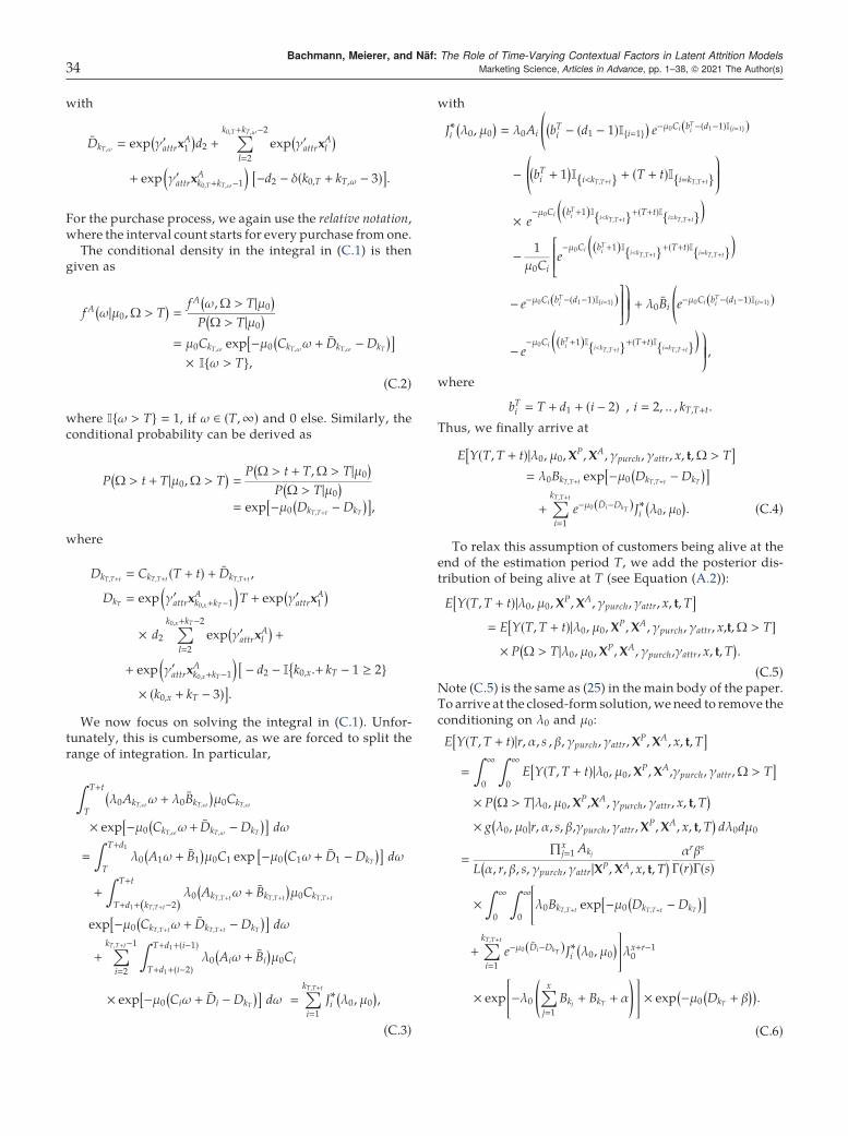
with

DkT,ω exp γ′attrx

A1

( )d2 +

∑k0,T+kT,ω−2

l2

exp γ′attrx

Al

( )

+ exp γ′attrx

Ak0,T+kT,ω−1

( )−d2 − δ k0,T + kT,ω − 3( )[ ]

.

For the purchase process, we again use the relative notation,where the interval count starts for every purchase from one.

The conditional density in the integral in (C.1) is thengiven as

fA ω|μ0,Ω > T( )

fA ω,Ω > T|μ0

( )

P Ω > T|μ0

( )

μ0CkT,ω exp −μ0 CkT,ωω + DkT,ω −DkT

( )[ ]

× I ω > T ,

(C.2)

where Iω > T 1, if ω ∈ (T,∞) and 0 else. Similarly, theconditional probability can be derived as

P Ω > t + T|μ0,Ω > T( )

P Ω > t + T,Ω > T|μ0

( )

P Ω > T|μ0

( )

exp −μ0 DkT,T+t −DkT

( )[ ],

where

DkT,T+t CkT,T+t T + t( ) + DkT,T+t ,

DkT exp γ′attrx

Ak0,x+kT−1

( )T + exp γ′

attrxA1

( )

× d2∑k0,x+kT−2

l2

exp γ′attrx

Al

( )+

+ exp γ′attrx

Ak0,x+kT−1

( )[− d2 − I k0,x

.+ kT − 1 ≥ 2

× k0,x + kT − 3( )].

We now focus on solving the integral in (C.1). Unfor-tunately, this is cumbersome, as we are forced to split therange of integration. In particular,

∫T+t

Tλ0AkT,ωω + λ0BkT,ω

( )μ0CkT,ω

× exp −μ0 CkT,ωω([

+ DkT,ω −DkT

)]dω

∫ T+d1

Tλ0 A1ω + B1

( )μ0C1 exp −μ0 C1ω + D1 −DkT

( )[ ]dω

+

∫T+t

T+d1+ kT,T+t−2( )λ0 AkT,T+tω + BkT,T+t

( )μ0CkT,T+t

exp −μ0 CkT,T+tω + DkT,T+t −DkT

( )[ ]dω

+∑kT,T+t−1

i2

∫ T+d1+ i−1( )

T+d1+ i−2( )

λ0 Aiω + Bi

( )μ0Ci

× exp −μ0 Ciω + Di −DkT

( )[ ]dω

∑kT,T+t

i1

J∗i λ0, μ0

( ),

(C.3)

with

J∗i λ0, μ0

( ) λ0Ai

(

bTi − d1 − 1( )I i1

( )e−μ0Ci bTi − d1−1( )I i1 ( )

−

(

bTi + 1( )

I i<kT,T+t + T + t( )I ikT,T+t

⎞⎟⎟⎟⎟⎟⎟⎟⎠

× e−μ0Ci bTi +1( )I

i<kT,T+t + T+t( )I

ikT,T+t

( )

−1

μ0Cie−μ0Ci bTi +1( )I

i<kT,T+t + T+t( )I

ikT,T+t

( )⎡⎢⎢⎢⎢⎢⎢⎢⎢⎢⎢⎢⎢⎢⎢⎢⎢⎢⎢⎣

− e−μ0Ci bTi − d1−1( )I i1 ( )⎤⎥⎥⎥⎥⎥⎥⎥⎥⎥⎥⎥⎥⎥⎥⎥⎥⎥⎥⎦

⎞⎟⎟⎟⎟⎟⎟⎟⎠ + λ0Bi

(

e−μ0Ci bTi − d1−1( )I i1 ( )

− e−μ0Ci bTi +1( )I

i<kT,T+t + T+t( )I

ikT,T+t

( )⎞⎟⎟⎟⎟⎟⎟⎟⎠,

where

bTi T + d1 + i − 2( ) , i 2, .. , kT,T+t.

Thus, we finally arrive at

E Y T,T + t( )|λ0, μ0,XP,XA, γpurch, γattr, x, t,Ω > T

[ ]

λ0BkT,T+t exp −μ0 DkT,T+t −DkT

( )[ ]

+∑kT,T+t

i1

e−μ0 Di−DkT( )J∗i λ0, μ0

( ). (C.4)

To relax this assumption of customers being alive at theend of the estimation period T, we add the posterior dis-tribution of being alive at T (see Equation (A.2)):

E Y T,T + t( )|λ0, μ0,XP,XA, γpurch, γattr, x, t,T

[ ]

E Y T,T + t( )|λ0, μ0,XP,XA, γpurch, γattr, x,

[t,Ω > T]

× P Ω > T|λ0, μ0,XP,XA, γpurch,

(γattr, x, t,T

).

(C.5)Note (C.5) is the same as (25) in the main body of the paper.To arrive at the closed-form solution, we need to remove theconditioning on λ0 and μ0:

E Y T,T + t( )|r, α, s , β, γpurch, γattr,XP,XA, x, t,T

[ ]

∫∞

0

∫∞

0

E Y T,T + t( )|λ0, μ0,XP,XA,

[γpurch, γattr,Ω > T

]

× P Ω > T|λ0, μ0,XP,

(XA, γpurch, γattr, x, t,T

)

× g λ0, μ0|r, α, s, β,(

γpurch, γattr,XP,XA, x, t,T

)dλ0dμ0

∏xj1 Akj


( ) αrβs

Γ r( )Γ s( )

×

∫∞

0

∫∞

0λ0BkT,T+t exp −μ0 DkT,T+t −DkT

( )[ ][

+∑kT,T+t

i1

e−μ0 Di−DkT( )J∗i λ0, μ0

( )]

λx+r−10

× exp −λ0

∑x

j1

Bkj + BkT + α

( )[ ]

× exp −μ0 DkT + β( )( )

.

(C.6)


To solve (C.6), we ignore the constant term for the mo-ment and look at the summands of the integral separately.First, we solve

∫∞

0

∫∞

0

λ0BkT,T+t exp −μ0 DkT,T+t −DkT

( )[ ]λx+r−10

exp −λ0

∑x

j1

Bkj + BkT + α

( )[ ]

exp −μ0 DkT + β( )( )

μs−10 dλ0dμ0

BkT,T+t

Γ x + r + 1( )∑x

j1 Bkj + BkT + α( )x+r+1

Γ s( )

DkT,T+t + β( )s .

(C.7)

We solve the second summand for i 1, . . . , kT,T+t. How-ever, we look at three cases separately: (1) i 2, . . . , kT,T+t − 1,(2) i 1, and (3) i kT,T+t.

Case 1. We first look at the middle part consisting ofi 2, . . . , kT,T+t − 1. The calculation is tedious, but straight-forward, as Γ(s)

Γ(s−1) s − 1:

∫∞

0

∫∞

0

e−μ0 Di−DkT( )J∗i λ0,μ0

( )λx+r−10 exp −λ0

∑x

j1

Bkj +BkT +α

( )[ ]

× exp −μ0 DkT +β( )( )

μs−10 dλ0dμ0

Γ x+ r+1( )Γ s−1( )

∑xj1Bkj +BkT +α

( )x+r+1

×Ai b

Ti s+1/Ci Di+β

( )[ ]+ Bi s−1( )

Di+β+CibTi( )s

[

−Ai bTi +1

( )s+1/Ci Di+β

( )[ ]+ Bi s−1( )

Di+β+Ci bTi +1( )( )s

]

:Γ x+ r+1( )Γ s−1( )

∑xj1Bkj +BkT +α

( )x+r+1Si.

Case 2. The first part i 1:

∫∞

0

∫∞

0e−μ0 D1−DkT( )J∗1 λ0,μ0

( )λx+r−10

exp −λ0

∑x

j1

Bkj +BkT +α

( )[ ]

exp −μ0 DkT +β( )( )

μs−10 dλ0dμ0

Γ x+ r+1( )Γ s−1( )

∑xj1Bkj +BkT +α

( )x+r+1

×A1 Ts+1/C1 D1+β

( )[ ]+ B1 s−1( )

D1+β+C1T( )s

[

−A1 T+d1( )s+1/C1 D1+β

( )[ ]+ B1 s−1( )

D1+β+C1 T+d1( )( )s

]

:Γ x+ r+1( )Γ s−1( )

∑xj1Bkj +BkT +α

( )x+r+1S∗1 .

Case 3. Finally for i kT,T+t,

∫∞

0

∫∞

0e−μ0 DkT,T+t

−DkT

( )J∗kT,T+t λ0, μ0

( )λx+r−10

× exp −λ0

∑x

j1

Bkj +BkT +α

( )[ ]

exp −μ0 DkT + β( )( )

μs−10 dλ0dμ0

Γ x+ r+ 1( )Γ s− 1( )

∑xj1 Bkj +BkT +α

( )x+r+1

×AkT,T+t b

TkT,T+t

s+ 1/Ci DkT,T+t + β( )[ ]

+ BkT,T+t s− 1( )

DkT,T+t + β+CkT,T+tbTkT,T+t

( )s

⎡⎢⎢⎢⎢⎢⎢⎢⎢⎢⎢⎢⎢⎢⎢⎢⎢⎢⎢⎢⎢⎢⎢⎢⎣

−AkT,T+t T + t( )s+ 1/CkT,T+t DkT,T+t + β

( )[ ]+ BkT,T+t s− 1( )

DkT,T+t + β+CkT,T+t T + t( )( )s

⎤⎥⎥⎥⎥⎥⎥⎥⎥⎥⎥⎥⎥⎥⎥⎥⎥⎥⎥⎥⎥⎥⎥⎥⎦

:Γ x+ r+ 1( )Γ s− 1( )

∑xj1 Bkj +BkT + α

( )x+r+1 S∗kT,T+t

.


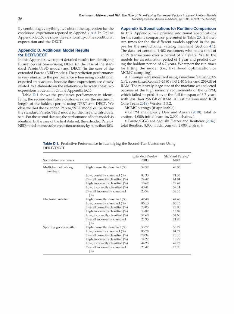
By combining everything, we obtain the expression for theconditional expectation reported in Appendix A.3. In OnlineAppendix EC.5, we show the relationship of the conditionalexpectation and the DECT.

Appendix D. Additional Model Results

for DERT/DECTIn this Appendix, we report detailed results for identifyingfuture top customers using DERT (in the case of the stan-dard Pareto/NBD model) and DECT (in the case of theextended Pareto/NBDmodel). The prediction performanceis very similar to the performance when using conditionalexpected transactions, because those expressions are closelyrelated. We elaborate on the relationship between these twoexpressions in detail in Online Appendix EC.5.

Table D.1 shows the predictive performance in identi-fying the second-tier future customers over the maximumlength of the holdout period using DERT and DECT. Weobserve that the extended Pareto/NBDmodel outperformsthe standard Pareto/NBDmodel for the first and third datasets. For the second data set, the performance of bothmodels isidentical. In the case of the first data set, the extended Pareto/NBDmodel improves thepredictionaccuracybymore than40%.

Appendix E. Specifications for Runtime ComparisonIn this Appendix, we provide additional specificationsfor the runtime comparison presented in Table 20. It showsrun times for the the different models applied in the pa-per for the multichannel catalog merchant (Section 4.1).The data set contains 1,402 customers who had a total of2,929 transactions over a period of 7.7 years. We fit themodels for an estimation period of 1 year and predict dur-ing the holdout period of 6.7 years. We report the run timesfor fitting the model (i.e., likelihood optimization orMCMC sampling).

All timings weremeasured using amachine featuring 32-CPU cores (Intel Xeon E5-2680 v4@ 2.40GHz) and 256GB ofRAM. The relatively large size of the machine was selectedbecause of the high memory requirements of the GPPM,which failed to predict over the full timespan of 6.7 yearswith less than 256 GB of RAM. All estimations used R (RCore Team 2018) Version 3.5.2.

MCMC settings (if applicable):• GPPM analogously Dew and Ansari (2018): total it-

eration, 4,000; initial burn-in, 2,000; chains, 1• Pareto/GGG analogously Platzer and Reutterer (2016):

total iteration, 8,000; initial burn-in, 2,000; chains, 4

Table D.1. Predictive Performance in Identifying the Second-Tier Customers UsingDERT/DECT

Second-tier customersExtended Pareto/

NBDStandard Pareto/

NBD

Multichannel catalogmerchant

High, correctly classified (%) 59.59 40.86

Low, correctly classified (%) 81.33 71.53Overall correctly classified (%) 74.47 61.84High, incorrectly classified (%) 18.67 28.47Low, incorrectly classified (%) 40.41 59.14Overall incorrectly classified

(%)25.54 38.16

Electronic retailer High, correctly classified (%) 47.40 47.40Low, correctly classified (%) 86.13 86.13Overall correctly classified (%) 78.05 78.05High, incorrectly classified (%) 13.87 13.87Low, incorrectly classified (%) 52.60 52.60Overall incorrectly classified

(%)21.95 21.95

Sporting goods retailer High, correctly classified (%) 55.77 50.77Low, correctly classified (%) 85.78 84.22Overall correctly classified (%) 78.34 76.10High, incorrectly classified (%) 14.22 15.78Low, incorrectly classified (%) 44.23 49.23Overall incorrectly classified

(%)21.47 23.90


References

Abe M (2009) Counting your customers one by one: A hierarchicalBayes extension to the Pareto/NBD model. Marketing Sci. 28(3):541–553.

Allenby GM, Leone RP, Jen L (1999) A dynamic model of purchasetiming with application to direct marketing. J. Amer. Statist.Assoc. 94(446):365–374.

Ascarza E, Iyengar R, Schleicher M (2016) The perils of proactivechurn prevention using plan recommendations: Evidence from afield experiment. J. Marketing Res. 53(1):46–60.

Bachmann P, Naef J, Schilter P, Kuebler N,MeiererM (2020) CLVTools:Tools for customer lifetime value estimation. Accessed September17, 2020, https://CRAN.R-project.org/package=CLVTools.

Braun M, Schweidel DA, Stein E (2015) Transaction attributes andcustomer valuation. J. Marketing Res. 52(6):848–864.

Colombo R, Jiang W (1999) A stochastic RFM model. J. InteractiveMarketing 13(3):2–12.

Dew R, Ansari A (2018) Bayesian nonparametric customer baseanalysis with model-based visualizations. Marketing Sci. 37(2):216–235.

Ebbes P, Papies D, van Heerde HJ (2011) The sense and non-sense ofholdout sample validation in the presence of endogeneity.Marketing Sci. 30(6):1115–1122.

Ehrenberg AS (1959) The pattern of consumer purchases. J. RoyalStatist. Soc. Ser. C. Appl. Statist. 8(March):26–41.

Ehrenberg AS (1988) Repeat-Buying: Facts, Theory, and Applications,2nd ed. (Charles Griffin and Company, London).

Fader PS (2012) Customer Centricity: Focus on the Right Customers forStrategic Advantage (Wharton Digital Press, Philadelphia).

Fader PS, Hardie BG (2005) A note on deriving the Pareto/NBDmodel and related expressions. Accessed September 17, 2020,http://www.brucehardie.com/notes/009/pareto_nbd_derivations_2005-11-05.pdf.

Fader PS, Hardie BG (2007) Incorporating time-invariant covariatesinto the Pareto/NBD and BG/NBD models. Accessed, http://www.brucehardie.com/notes/019/time_invariant_covariates.pdf.

Fader PS, Hardie BG, Lee K (2005a) Counting your customers theeasy way: An alternative to the Pareto/NBD model. MarketingSci. 24(2):275–284.

Fader PS, Hardie BG, Lee K (2005b) RFM and CLV: Using iso-valuecurves for customer base analysis. J. Marketing Res. 42(4):415–430.

Fader PS, Hardie BGS, Shang J (2010) Customer-base analysis ina discrete-time noncontractual setting. Marketing Sci. 29(6):1086–1108.

Glady N, Lemmens A, Croux C (2015) Unveiling the relationshipbetween the transaction timing, spending and dropout behaviorof customers. Internat. J. Res. Marketing 32(1):78–93.

Gopalakrishnan A, Bradlow ET, Fader PS (2017) A cross-cohortchangepoint model for customer-base analysis. Marketing Sci.36(2):195–213.

Gupta S (1991) Stochastic models of interpurchase time with time-dependent covariates. J. Marketing Res. 28(1):1–15.

Hanssens DM, Pauwels KH (2016) Demonstrating the value ofmarketing. J. Marketing 80(6):173–190.

Harman DM (2016) Stochastic process customer lifetime valuemodels with time-varying covariates. Dissertation, University ofIowa, Iowa City.

Hruschka H (2010) Considering endogeneity for optimal catalogallocation in direct marketing. Eur. J. Oper. Res. 206(1):239–247.

Jerath K, Fader PS, Hardie BGS (2011) New perspectives on customerdeath using a generalization of the Pareto/NBD model. Mar-keting Sci. 30(5):866–880.

Jeuland AP, Bass FM, Wright GP (1980) A multibrand stochasticmodel compounding heterogeneous Erlang timing and multi-nomial choice processes. Oper. Res. 28(2):255–277.

Knox G, van Oest R (2014) Customer complaints and recovery ef-fectiveness: A customer base approach. J. Marketing 78(5):42–57.

Kuhn HW, Tucker AW (1951) Nonlinear programming. Neyman J,ed. 2nd Berkeley Sympos. Math. Statist. Probab.y (University ofCalifornia Press, Berkeley), 481–492.

Malthouse EC (2009) The results from the lifetime value and cus-tomer equitymodeling competition. J. Interactive Marketing 23(3):272–275.

Marketing EDGE (2013) Specialty multi-channel catalog company.Accessed September 17, 2020, http://www.marketingedge.org/marketing-programs/data-set-library.

McCarthy D, Fader P (2018) Customer-based corporate valuation forpublicly traded non-contractual firms. J. Marketing Res. 55(5):617–635.

Neslin SA, Rhoads EE (2009) A model and empirical analysis ofpatient compliance and persistence in pharmaceuticals. Workingpaper, Dartmouth College, Dartmath, MA.

Netzer O, Lattin JM, Srinivasan V (2008) A hidden Markov model ofcustomer relationship dynamics. Marketing Sci. 27(2):185–204.

Ni J, Neslin AS, Sun B (2012) The ISMS durable goods data sets.Marketing Sci. 31(6):1008–1013.

Park S, Gupta S (2012) Handling endogenous regressors by jointestimation using copulas. Marketing Sci. 31(4):567–586.

Petrin A, Train K (2010) A control function approach to endogeneityin consumer choice models. J. Marketing Res. 47(1):3–13.

Platzer M (2018) BTYDplus: Probabilistic models for assessing andpredicting your customer base. Accessed September 17, 2020,https://github.com/mplatzer/BTYDplus#readme.

Platzer M, Reutterer T (2016) Ticking away the moments: Timingregularity helps to better predict customer activity.Marketing Sci.35(5):779–799.

R Core Team (2018) R: A Language and Environment for StatisticalComputing (R Foundation for Statistical Computing, Vienna).

Reinartz WJ, Kumar V (2000) On the profitability of long-life cus-tomers in a noncontractual setting: An empirical investigationand implications for marketing. J. Marketing 64(4):17–35.

Reinartz WJ, Kumar V (2003) The impact of customer relationshipcharacteristics on profitable lifetime duration. J. Marketing 67(1):77–99.

Rivers D, Vuong Q (1988) Limited information estimators and exo-geneity tests for simultaneous probit models. J. Econometrics39(3):347–366.

Ross SM (2014) Introduction to Probability Models, 11th ed. (Elsev-ier, Amsterdam).

Schmittlein DC, Peterson RA (1994) Customer base analysis: An in-dustrial purchase process application. Marketing Sci. 13(1):41–67.

Schmittlein DC, Bemmaor AC, Morrison DG (1985) Why does theNBD model work? Robustness in representing product pur-chases, brand purchases and imperfectly recorded purchases.Marketing Sci. 4(3):255–266.

Schmittlein DC, Morrison DG, Colombo R (1987) Counting yourcustomers: Who are they and what will they do next? Man-agement Sci. 33(1):1–24.

Schroeder N, Hruschka H (2016) Investigating the effects of mailingvariables and endogeneity onmailing decisions. Eur. J. Oper. Res.250(2):579–589.

Schweidel DA, Knox G (2013) Incorporating direct marketing activityinto latent attrition models. Marketing Sci. 32(3):471–487.

Shugan SM (2004) Endogeneity in marketing decision models.Marketing Sci. 23(1):1–3.

Singh SS, Jain DC (2013) Measuring Customer Lifetime Value:Models and Analysis. INSEAD Working Paper No. 2013/27/MKT, http://www.ssrn.com/abstract=2214860.

Singh SS, Borle S, Jain DC (2009) A generalized framework for es-timating customer lifetime valuewhen customer lifetimes are notobserved. Quant. Marketing Econom. 7(2):181–205.


https://CRAN.R-project.org/package=CLVTools

http://www.brucehardie.com/notes/009/pareto_nbd_derivations_2005-11-05.pdf

http://www.brucehardie.com/notes/009/pareto_nbd_derivations_2005-11-05.pdf

http://www.brucehardie.com/notes/019/time_invariant_covariates.pdf

http://www.brucehardie.com/notes/019/time_invariant_covariates.pdf

http://www.marketingedge.org/marketing-programs/data-set-library

http://www.marketingedge.org/marketing-programs/data-set-library

https://github.com/mplatzer/BTYDplus#readme

http://www.ssrn.com/abstract=2214860

VanOest R, KnoxG (2011) Extending the BG/NBD:A simplemodel ofpurchases and complaints. Internat. J. Res. Marketing 28(1):30–37.

Wooldridge JM (2015) Control function methods in applied econo-metrics. J. Human Resources 50(2):420–445.

Wübben M, Wangenheim F (2008) Instant customer base analysis:Managerial heuristics often “get it right”. J. Marketing 72(3):82–93.

Wünderlich R (2015) Hierarchical Bayesian models for predictingpurchase behavior in noncontractual settings based on individual

and cross-sectional purchase patterns. Dissertation, TechnischeUniversitat München, Germany.

Xia F, Chatterjee R, May JH (2019) Using conditional restrictedBoltzmann machines to model complex consumer shoppingpatterns. Marketing Sci. 38(4):711–727.

Zhang Y, Bradlow ET, Small DS (2015) Predicting customer valueusing clumpiness: From RFM to RFMC. Marketing Sci. 34(2):195–208.


Documents

The Role of Time-Varying Contextual Factors in Latent