The role of specific cations and water entropy on the stability of branched DNA motif structures

Tod A Pascal, William A Goddard III, Prabal K Maiti and Nagarajan Vaidehi

Supporting Information

1. Figures

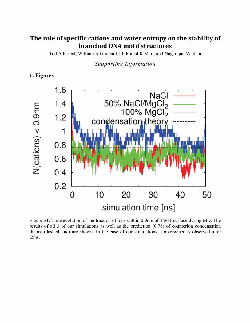
Figure S1. Time evolution of the fraction of ions within 0.9nm of TWJ1 surface during MD. The results of all 3 of our simulations as well as the prediction (0.78) of counterion condensation theory (dashed line) are shown. In the case of our simulations, convergence is observed after 25ns.

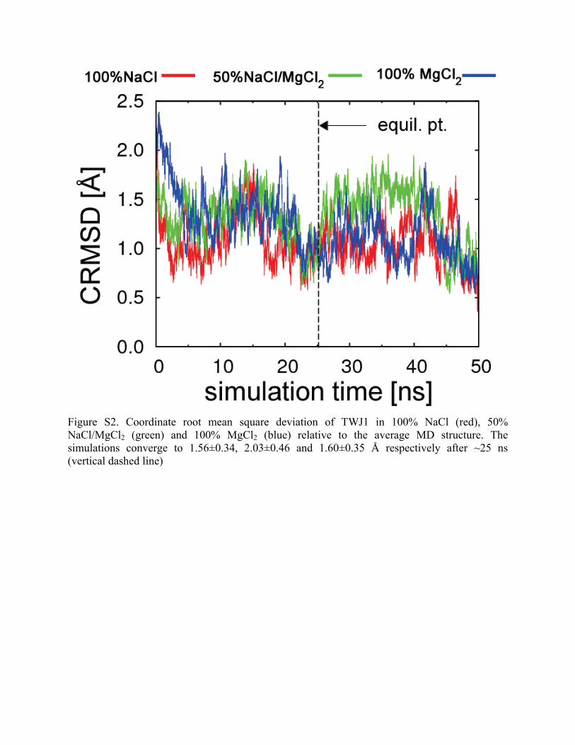
Figure S2. Coordinate root mean square deviation of TWJ1 in 100% NaCl (red), 50% NaCl/MgCl2 (green) and 100% MgCl2 (blue) relative to the average MD structure. The simulations converge to 1.56±0.34, 2.03±0.46 and 1.60±0.35 Å respectively after ~25 ns (vertical dashed line)

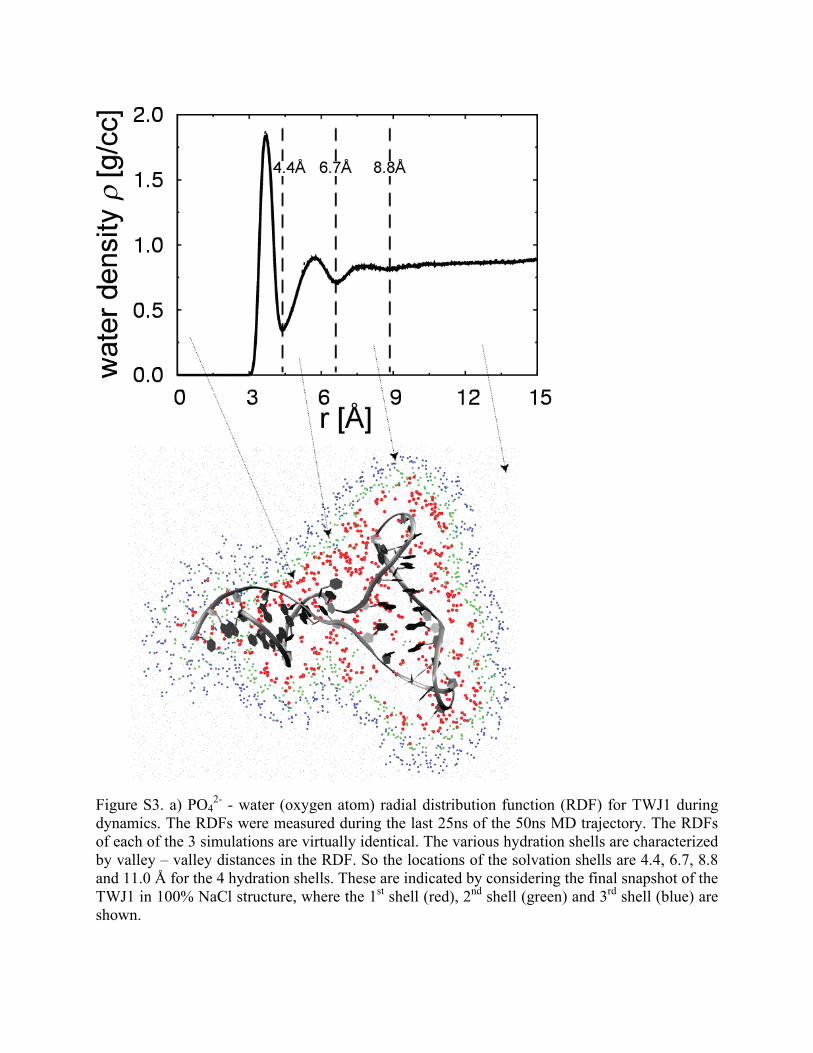
Figure S3. a) PO42- - water (oxygen atom) radial distribution function (RDF) for TWJ1 during

dynamics. The RDFs were measured during the last 25ns of the 50ns MD trajectory. The RDFs of each of the 3 simulations are virtually identical. The various hydration shells are characterized by valley – valley distances in the RDF. So the locations of the solvation shells are 4.4, 6.7, 8.8 and 11.0 Å for the 4 hydration shells. These are indicated by considering the final snapshot of the TWJ1 in 100% NaCl structure, where the 1st shell (red), 2nd shell (green) and 3rd shell (blue) are shown.

2. Tables.

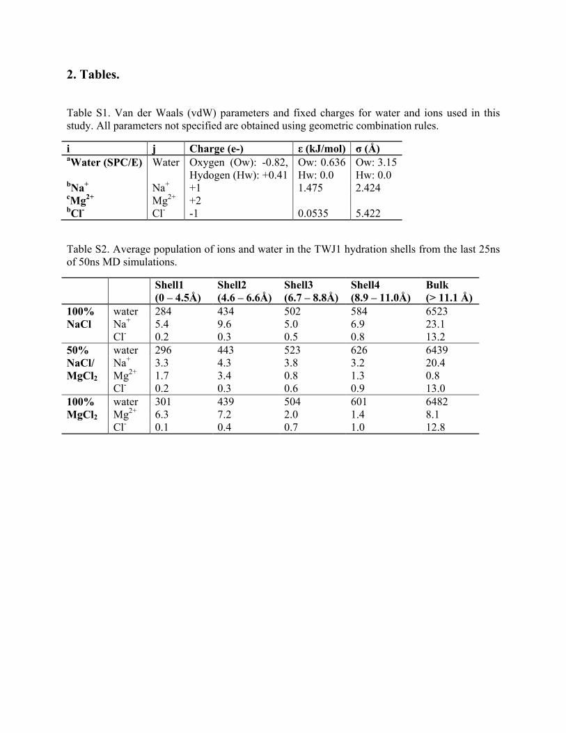
Table S1. Van der Waals (vdW) parameters and fixed charges for water and ions used in this study. All parameters not specified are obtained using geometric combination rules.

i j Charge (e-) ε (kJ/mol) σ (Å) aWater (SPC/E) Water Oxygen (Ow): -0.82,

Hydogen (Hw): +0.41 Ow: 0.636 Hw: 0.0

Ow: 3.15 Hw: 0.0

bNa+ Na+ +1 1.475 2.424 cMg2+ Mg2+ +2 bCl- Cl- -1 0.0535 5.422

Table S2. Average population of ions and water in the TWJ1 hydration shells from the last 25ns of 50ns MD simulations.

Shell1 (0 – 4.5Å)

Shell2 (4.6 – 6.6Å)

Shell3 (6.7 – 8.8Å)

Shell4 (8.9 – 11.0Å)

Bulk (> 11.1 Å)

100% NaCl

water 284 434 502 584 6523 Na+ 5.4 9.6 5.0 6.9 23.1 Cl- 0.2 0.3 0.5 0.8 13.2

50% NaCl/ MgCl2

water 296 443 523 626 6439 Na+ 3.3 4.3 3.8 3.2 20.4 Mg2+ 1.7 3.4 0.8 1.3 0.8 Cl- 0.2 0.3 0.6 0.9 13.0

100% MgCl2

water 301 439 504 601 6482 Mg2+ 6.3 7.2 2.0 1.4 8.1 Cl- 0.1 0.4 0.7 1.0 12.8

Table S3. Thermodynamics of TWJ1 systems

Pure NaCl nmol <G> kJ/mol <H> kJ/mol <S> J/mol/K avg std Avg std avg std avg std Shell1 284 15 -53.8 0.1 -36.3 0.1 58.7 0.5 Shell2 434 20 -53.9 0.1 -34.0 0.1 67.0 0.4 Shell3 502 26 -54.1 0.1 -34.7 0.1 65.2 0.3 Shell4 584 29 -54.1 0.1 -34.6 0.1 65.4 0.3 Bulk 6523 50 -54.0 0.0 -34.5 0.0 65.5 0.2 DNA 1 -25055.0 89.1 -21890.1 103.5 10807.1 85.7 Na+ 50 -405.7 0.9 -392.8 0.8 43.1 0.9 Cl- 15 -392.9 1.1 -373.4 0.9 65.0 2.0 50% NaCl/MgCl2 Shell1 296 17 -55.5 0.2 -38.2 0.2 58.0 0.5 Shell2 443 19 -55.2 0.2 -35.0 0.2 67.7 0.4 Shell3 523 25 -54.2 0.1 -34.8 0.2 65.1 0.3 Shell4 626 32 -54.1 0.1 -34.6 0.1 65.3 0.3 Bulk 6439 50 -54.0 0.0 -34.5 0.0 65.3 0.2 DNA 1 -26829.2 97.4 -23642.1 111.8 10873.5 89.1 Na+ 34 -406.4 0.8 -393.0 0.8 44.5 1.1 Cl- 15 -392.7 1.0 -373.2 1.0 65.2 1.9 Mg2+ 8 -1629.4 2.4 -1622.0 2.3 24.9 1.5 Pure MgCl2 Shell1 301 16 -58.3 0.4 -42.2 0.4 54.1 0.5 Shell2 439 19 -57.2 0.3 -37.5 0.3 66.1 0.4 Shell3 504 24 -55.3 0.2 -36.8 0.3 61.9 0.4 Shell4 601 25 -55.1 0.2 -36.5 0.2 62.3 0.3 Bulk 6482 38 -55.0 0.1 -36.4 0.1 62.5 0.2 DNA 1 -24301.2 93.9 -21226.0 105.9 10502.4 88.9 Mg2+ 25 -1650.5 1.6 -1642.9 1.6 25.3 0.9 Cl- 15 -393.8 1.0 -375.1 1.0 62.5 1.8

Table S4. Analysis of rotational (Srot) and translational (Strans) water entropy (J/mol/K) in various solvation shells around TWJ1.

pure NaCl 50% NaCl/MgCl2 pure MgCl2 avg std avg std avg std Srot Shell 1 9.89 0.10 9.68 0.10 8.93 0.10 Shell 2 12.48 0.09 12.39 0.09 12.61 0.08 Shell 3 10.54 0.08 10.50 0.08 9.78 0.07 Shell 4 10.54 0.06 10.50 0.07 9.81 0.07 Bulk 10.53 0.04 10.51 0.05 9.81 0.04 Water boxa 10.41 0.04 Strans Shell 1 48.76 0.45 48.27 0.43 45.15 0.44 Shell 2 54.48 0.33 55.27 0.35 53.51 0.34 Shell 3 54.67 0.30 54.56 0.30 52.15 0.31 Shell 4 54.90 0.27 54.77 0.27 52.53 0.28 Bulk 54.99 0.14 54.81 0.13 52.67 0.14 Water box 49.87 0.14 aReference 1

3. Methods Estimating of the system thermodynamics from MD simulations

3.a.i. Solids: Debye theory of solids

The canonical partition function Q of a system is related to the entropy S, internal energy E, Helmholtz free energy A and constant volume heat capacity Cv by2

2

ln ln (1)

ln

ln

B B

B

B

v

QS k T k QT

QE k TT

A E TS k T QECT

∂= +

∂∂

=∂

= − = −∂

=∂

where kB is Boltzmann’s constant. In the harmonic limit, one approximates the normal modes of a system as a set of 3N harmonic oscillators, so that the partition function Q can be expressed in term of the partition function qi for the individual modes3:

3

1

(2.1)N

ii

Q q=

=∏

or

3

1ln (2.2)

N

ii

Q q=

=∑

and for a continuous distribution of normal frequencies

( ) ( )0

ln ln (2.3)Q DoS v q v dv∞

= ∫

where DoS(v) is the density of states function at frequency v. The DoS(v) can be extracted directly from a MD trajectory as the Fourier transform of the integrated atomic velocity autocorrelation function (VACF) C(t):

( ) ( ) ( )1lim exp 2 (3.1)2

DoS v C t vt dtkT

τ

ττ

π→∞

−

= −∫

where

( ) ( ) ( )3

1 1

1lim ' ' (3.2)2

N j ji i ii j

C t m v t t v t dtτ

ττ τ= = −→∞

= + ∑ ∑ ∫

mi is the mass and ( )jiv t is the j-th component of the velocity of atom i at time t. Thus all that

remains to extract the thermodynamics in eqn (1) is the weighting function q(v) in 2.3, which becomes that of a quantum harmonic oscillator2

( ) ( )( )

exp 2(4)

1 exphv

q vhv

ββ

−=

− −

where β = 1/kBT is the energy of the harmonic oscillator at temperature T.

2.a.ii. Gases: Carnahan-Starling hard sphere

For a hard-sphere gas of N particles at constant pressure P and temperature T, the VACF decays exponentially2

( ) ( ) ( ) ( )30 exp exp (5.1)gas gas kTC t C t tm

α α= − = −

and

( ) ( ) ( )0

4 3 exp cos 2 (5.2)DoS v NkT t vt dtkT

α π∞

= −∫

where α is the Enskog friction constant related to the collisions between hard spheres. The absolute thermodynamics can then be obtained from integrating (5.2) with the appropriate weighting functions:

0.5 (6)

3

1.53

E vgas

SB

gasB

AB

W CSW

kk TSW E TS

k

= =

=

−= − =

where Sgas can be obtained from the accurate Carnahan–Starling equation of state4:

( ) ( )( )

( )( )

2

2 3

3

3 4ln (7)

1

11

gasB

y yS k z y

y

y y yz yy

− = + − + + −

=−

where y is the hard-sphere packing fraction defined as 3 6y πρσ= .

3.a.iii. Liquids: 2PT method for condensed phase systems

By inspection, one observes that substituting eqn (4) into (2.3) results in a singularity at v = 0 for a finite DoS(0). While a DoS(0) = 0 for a solid, in a liquid and generally for strongly interacting systems, DoS(0) > 0 due to diffusion

( ) 120 (8)B

mNDDoSk T

=

where D is the self-diffusion constant. One method of addressing this issue is the Two-Phase Thermodynamics (2PT) method1,5 which is based on the Lin, Blanco and Goddard (LBG) theory of condensed phase thermodynamics. The 2PT method builds on an idea first proposed by Eyring and Rae6 whereby the DoS function of a liquid is expressed as a linear combination of a gas (eqn 5.2) and a solid (eqn 2.3):

( ) ( ) ( ) ( )1 (9)tot gas solidDoS v fDoS v f DoS v= + −

where f, termed the “fluidicity” factor, is the number of diffusive modes in the system. Thus as implemented in 2PT, LGB showed that by setting DoStot(0) = DoSgas(0), DoSsolid(0) = 0, the singularity in eqn 4 is avoided and the thermodynamics obtained by integrating with the appropriate weighting functions in eqn 1 and 6. All that remained is to define the f factor. Thus a defining feature of LBG theory is that f can be determined self-consistently from the MD trajectory

( ) ( ) 120 0 (10.1)tot gasfNDoS DoSα

= =

since f is related to the packing fraction y by1

( ) ( )3 3 2 22 6 2 6 2 0 (10.2)y f y y f y f− + + + − =

3.b. Application to real systems

For strongly coupled system such as liquids, there are quantifiable differences in the zero-point energy motions, enthalpy and heat capacity of the system described quantum-mechanically (with discrete energy states) and classically (with a continuum of states), where the quantum description being closer to the experimental reality. These quantum effects are especially important in accurately describing the physics of water7, even at room temperature where one would expect the effect to by minimal8. In lieu of performing prohibitive quantum dynamics, one can approximate the quantum effects from classical trajectories by Feyman-Hibbs9 path integral techniques10, or by the Wigner-Kirkwod technique11,12 of adding the first term in the power series expansion of the energy in h2 to the classical values. An alternative approached introduced by Berens et al3 approximates the quantum effects as the difference in the DoS using the weighting function of the quantum harmonic oscillator in Eqn. 4 and the classical harmonic

oscillator ( ) ( ) 1Cq v hvβ −= . Thus in addition to providing an efficient estimate of the quantum molar entropy, the 2PT method allows for the approximation of quantum effects in the internal energy U:

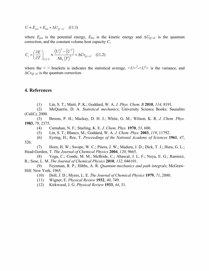
(11.1)pot kin Q CU E E U −>≈ + + ∆

where Epot is the potential energy, Ekin is the kinetic energy and ∆UQ→C is the quantum correction, and the constant volume heat capacity Cv

2 2

2, ,

(11.2)v Q CN V T b

U UEC CvT Nk T −>

−∂ = ≈ + ∆ ∂

where the < > brackets is indicates the statistical average, <U>2-<U2> is the variance, and ∆CvQ→C is the quantum correction.

4. References

(1) Lin, S. T.; Maiti, P. K.; Goddard, W. A. J. Phys. Chem. B 2010, 114, 8191. (2) McQuarrie, D. A. Statistical mechanics; University Science Books: Sausalito (Calif.), 2000. (3) Berens, P. H.; Mackay, D. H. J.; White, G. M.; Wilson, K. R. J. Chem. Phys. 1983, 79, 2375. (4) Carnahan, N. F.; Starling, K. E. J. Chem. Phys. 1970, 53, 600. (5) Lin, S. T.; Blanco, M.; Goddard, W. A. J. Chem. Phys. 2003, 119, 11792. (6) Eyring, H.; Ree, T. Proceedings of the National Academy of Sciences 1961, 47, 526. (7) Horn, H. W.; Swope, W. C.; Pitera, J. W.; Madura, J. D.; Dick, T. J.; Hura, G. L.; Head-Gordon, T. The Journal of Chemical Physics 2004, 120, 9665. (8) Vega, C.; Conde, M. M.; McBride, C.; Abascal, J. L. F.; Noya, E. G.; Ramirez, R.; Sese, L. M. The Journal of Chemical Physics 2010, 132, 046101. (9) Feynman, R. P.; Hibbs, A. R. Quantum mechanics and path integrals; McGraw-Hill: New York, 1965. (10) Doll, J. D.; Myers, L. E. The Journal of Chemical Physics 1979, 71, 2880. (11) Wigner, E. Physical Review 1932, 40, 749. (12) Kirkwood, J. G. Physical Review 1933, 44, 31.