RFF REPORT

The Role of Land Use in Adaptation to Increased Precipitation and Flooding:

A Case Study in Wisconsin’s Lower Fox River Basin

Carolyn Kousky, Sheila Olmstead, Margaret Walls, Adam Stern, and Molly Macauley

NOVEMBER 2011

Table of Contents

Executive Summary............................................................................................................................................... i

1. Introduction and Motivation ........................................................................................................................ 1

2. Background on Study Area ........................................................................................................................... 4

2.1. Introduction ............................................................................................................................................... 4

2.2. Population, Income, and Land Use in Lower Fox River Basin ................................................ 4

2.3. History of Extreme Precipitation and Flooding in the LFRB ................................................... 7

2.4. Water Quality Problems in the River Basin ................................................................................ 10

2.5. The East River Watershed ................................................................................................................. 11

3. Climate Change in the Great Lakes Area .............................................................................................. 14

3.1. Future Temperature and Precipitation in the Great Lakes Region ................................... 14

3.2. Extreme Precipitation in the Great Lakes Region .................................................................... 16

3.3. Projected Economic Impacts from Changes in Extreme Precipitation ............................ 18

4. Modeling and Estimating the Economic Costs of Flooding ........................................................... 20

4.1. Estimating Flood Damages with Hazus ........................................................................................ 20

4.2. Improving Estimation with Hazus .................................................................................................. 22

4.3. Flood Damages in the East River Watershed ............................................................................. 23

4.4. Who Pays for Flood Damage? ........................................................................................................... 30

5. Policy Options Other Than Land Use for Reducing Flood Damages .......................................... 34

5.1. Structural Flood Control..................................................................................................................... 34

5.2. Insurance .................................................................................................................................................. 34

5.3. Building Regulations ............................................................................................................................ 35

5.4. Warnings and Evacuation .................................................................................................................. 36

6. Land-Use Options for Mitigating Flood Damage ............................................................................... 36

6.1. Wetlands as Reservoirs ...................................................................................................................... 36

© 2011 Resources for the Future. Resources for the Future is an independent, nonpartisan think tank that, through its social science research, enables policymakers and stakeholders to make better, more informed decisions about energy, environmental, and natural resource issues. Headquartered in Washington, DC, its research scope comprises programs in nations around the world.

FAGAN AND DEFRIES 1

6.2. Pervious Surface Area and Infiltration ......................................................................................... 37

6.3. Reducing Exposure ............................................................................................................................... 37

7. Comparing the Benefits of Flood Damage Mitigation with the Costs ........................................ 37

7.1. The Benefits of Avoided Flood Damages ..................................................................................... 38

7.2. The Costs of Avoided Flood Damages ........................................................................................... 40

7.3. Improving Efficiency and Cost-effectiveness: Better Targeting of Parcels .................... 45

8. Co-Benefits and Co-Damages Associated with Flood Damage Mitigation Policies .............. 46

8.1. Effects on Water Quality ..................................................................................................................... 46

8.2. Monetizing Water Quality Co-Benefits or Co-Damages ......................................................... 48

8.3. Recreational and Other Co-Benefits Directly from Land-Use Change .............................. 52

8.4. Monetizing Recreation and Other Co-Benefits from Open Space ....................................... 52

9. Policy Tools for Changing Land Use ....................................................................................................... 55

9.1 Purchase of Development Rights ..................................................................................................... 55

9.2. Transfer of Development Rights ..................................................................................................... 56

9.3. Development Fees or Taxes .............................................................................................................. 57

9.4. Zoning ........................................................................................................................................................ 58

9.5. Summary of Policy Instruments ...................................................................................................... 58

9.6. Funding Opportunities for Wisconsin Fee Simple Land Purchase and PDR Programs .......................................................................................................................................................... 58

10. Conclusions ................................................................................................................................................... 62

Acknowledgments ............................................................................................................................................. 64

References ............................................................................................................................................................ 65

i KOUSKY ET AL.

THE ROLE OF LAND USE IN ADAPTATION TO INCREASED

PRECIPITATION AND FLOODING: A CASE STUDY IN

WISCONSIN’S LOWER FOX RIVER BASIN Carolyn Kousky, Sheila Olmstead, Margaret Walls, Adam Stern,

and Molly Macauley*

Executive Summary

limate models predict that storms and flooding will increase in frequency and severity in some

regions. In light of these predictions, and with appreciation for the great uncertainty in these

forecasts, communities will be looking for ways to improve their resilience to extreme events.

Protection of natural areas and open space is one option.

Strategically protecting natural lands and open space can reduce damages from flooding and

also provide environmental and social benefits, including improved water quality in streams and

rivers, protection of groundwater sources, and enhanced recreational opportunities. Governments

around the world are increasingly recognizing that “green infrastructure” can often be a cost-

effective substitute for the gray infrastructure—pipes, dams, levees—traditionally used to control

flooding.

Nevertheless, many questions remain for communities. How much land should be protected,

and where? How does the community balance flood protection and the co-benefits of green

infrastructure in choosing which lands to target? And how does it maximize the net benefits of the

actions—the benefits of flood protection, water quality, recreation, and so forth, minus the costs of

protecting the land from development? Finally, how can the local government bring about this land-

use change? What policies and approaches are feasible and cost-effective?

We address such questions in a case study of the Lower Fox River basin in Wisconsin. The

Lower Fox River flows northeast from central Wisconsin to Green Bay, the largest freshwater

estuary in the world. Water quality here has been a problem for decades, and many areas

experience flooding. Scientists predict that these problems will worsen in the future with climate

change: extreme precipitation events are expected to increase, leading to more flooding and

exacerbating water pollution. Moreover, some parts of the basin are experiencing development

pressures. The impervious surfaces that come with development tend to intensify flooding and

some water quality problems, and flooding damages increase with the number of buildings located

in floodplains.

* Kousky, Fellow, Resources for the Future (RFF); Olmstead, Fellow, RFF; Walls, Senior Fellow and Thomas Klutznick Chair, RFF; Adam Stern, Research Assistant, RFF; Molly Macauley, Vice Presdient for Research and Senior Fellow, RFF.

C

ii KOUSKY ET AL.

Local government planners in other areas facing similar issues will find a framework here for

determining the costs and benefits of using land-use policy to mitigate flood damage. While the case

study is specific to Wisconsin, the methodology applies equally to other locations.

Background Information on the Lower Fox River Basin

Current and Projected Land Use

Less than 15 percent of the land in the Lower Fox River basin is in natural uses, such as

wetlands and forests, and more than half is used for agriculture. Sediment and nutrients, such as

nitrogen and phosphorus, cause eutrophication, toxic algae blooms, and reductions in water clarity

in Green Bay. These problems can necessitate beach closures, diminish the quality of recreation,

and harm both commercial and recreational fishing by contributing to fish mortality.

Local governments predict that population growth—nearly 55,000 additional new residents by

2025—will create demand for approximately 21,000 acres of new residential development and

2,450 acres of commercial development in Brown County, in the eastern portion of the river basin.

Residential, commercial, and industrial land uses are expected to increase by 46 percent over this

period, much of it in the floodplain.

Expected Changes in Climate and Their Consequences

Scientific research suggests that climate change is already taking place in the Great Lakes

region. For the past three decades, temperatures and precipitation have often been above average.

Most researchers agree that the frequency and severity of extreme precipitation events will rise,

increasing the risk of flooding and the expected damages to buildings and infrastructure in flood

zones. In addition, greater average annual precipitation and more extreme events will increase the

total urban and agricultural runoff into rivers and lakes, exacerbating water quality problems.

Modeling Flood Damage

Flooding damages structures, their contents, infrastructure, and crops. The costs of flooding

also include debris cleanup, loss of income when businesses shut down, emergency response costs,

and temporary housing costs for displaced people. We estimate flood damages with Hazus, a GIS-

based model developed for the Federal Emergency Management Agency (FEMA) to help local

officials and emergency planners estimate losses from floods, earthquakes, and hurricanes. For

flooding, Hazus relies on a digital elevation model to delineate the stream network for a region and

draws from national databases of the inventory of structures at the census block level and for

critical facilities at the site-specific level. Depth-damage curves, which link the depth of flooding to

the amount of damage to a structure and its contents, are coupled with the flood surface elevation

layer to estimate physical damages. These vary by occupancy class and building material.

Hazus can operate at three levels depending on the needs and expertise of the user. A Level 1

analysis uses default data and models. A Level 2 analysis integrates detailed user-supplied data. In a

Level 3 analysis, the user can import results from third-party studies that offer a more sophisticated

hydrological analysis. As one moves to higher levels, the results of the model become more precise.

In this study, we undertake a Level 2 analysis.

iii KOUSKY ET AL.

Baseline and Development Scenario Model Runs

The East River watershed in the Lower Fox River basin lies almost entirely within Brown

County and is an area notable for flooding problems and water quality concerns. Moreover, it is one

of the areas with the most serious development pressures. We focus our benefit-cost analysis on

this watershed. We model baseline flood damage estimates for 10-year, 50-year, 100-year, and

500-year flood events in terms of total building, content, and inventory loss; business interruption

loss; the number of moderately damaged buildings; the truckloads of debris generated; the number

of displaced households; and agricultural losses—all based on the current (2010) land-use pattern.

Total building, content, and inventory losses range from $47.5 million for a 10-year flood event to

almost $109 million for a 500-year flood. These losses all appear to be larger than the damages

sustained in the area during recent floods. For example, 1990 flood damages were estimated at $11

million (in 2009 dollars). Intuitively, the areas of greatest damage occur where flooding is deeper

and more extensive and structures are more numerous.

The county’s forecasts of growth are the basis for the future development scenario. The county

provided a geographic information (GIS) file of expected land uses in the county in 2025. The

amount of land in developed uses is predicted to increase by 35 percent over the 2010 baseline.

When we run Hazus for 10-, 50-, 100-, and 500-year floods with expected future development,

building losses increase, depending on the event, by roughly $8 million to $13 million. Total

building, content, and inventory losses, for example, range from about $60 million to $124 million.

For both the 2010 and future development model runs, we had to convert GIS parcel-level data

from Brown County into a database of building counts and exposure at the census block level for

the 32 building occupancy classes in Hazus. For the 2010 runs, this was done using maps of land

use coupled with information from the tax assessor’s office on the value of properties. We had to

match each land use type for each property in the Brown County data to the 32 classes in Hazus.

For the future runs, we used the projection of future land use, coupled with the 2010 parcel map

and assessor’s data. We identified all parcels that were natural areas or agricultural land in 2010

but expected to be developed in the future. After mapping the future land uses to Hazus categories,

each parcel was assigned the mean value of that class in the watershed from the 2010 assessor’s

information. From this, counts and values were aggregated to the census block level, and the Hazus

inventory was updated.

A drawback of using a level-2 Hazus analysis in this way is that the hydrology does not update if

impervious surface area changes. So our future development scenario runs are based solely on

increased damages from building in flood-prone areas. If the development also increases runoff and

flood risk outside the current floodplain, or if it causes deeper flooding within the current

floodplain, or if return intervals change and severe floods become more frequent, the damages

could be greater than our estimates suggest.

The Potential for Green Infrastructure to Reduce Flood Damages

Green infrastructure can reduce flood damages in several ways. First, restoring or preserving

wetlands can lower flood damages because wetlands can be a natural sponge, absorbing

floodwaters. Research has found that having wetland areas of only 5 to 10 percent can reduce peak

stream flows by 50 percent compared with the case of no wetlands. Second, water can be stored in

the soil column, so increasing greenways can allow some water to infiltrate into the ground,

iv KOUSKY ET AL.

reducing runoff. Carefully constructed and located rain gardens, detention basins, and bioswales

that mimic natural hydrology can increase infiltration and slow runoff. Third, by removing

structures from the floodplain, there is less property to damage in the event of a flood. This last

impact is the one we focus on through our Hazus modeling in this study. We present alternative

green infrastructure scenarios and provide a rough estimate of the costs of each scenario.

Costs and Benefits of Using Land Conservation to Reduce Flood Damages

In the report, we present a framework for analyzing the benefits and costs of land conservation

in the floodplain as a means of mitigating the damages from flooding. We present benefit and cost

estimates for targeting land parcels for preservation. We take as our starting point a comparison of

expected flood damages for today’s land-use patterns with those for the future scenario, in which

more land in the watershed is in developed uses. If the lands projected to be developed are instead

protected as natural areas or remain in agricultural use, flood damages will be lower. These avoided

damages are our estimates of the flood benefits of land conservation. The costs are the expense of

protecting open space. Here, a government can take many approaches. Two of the most common

are: it can purchase land and retain it as publicly owned and managed open space or parkland, or it

can purchase easements that keep the land in private ownership but restrict residential or

commercial development.

We do not perform a definitive benefit-cost calculation for the East River watershed. Rather, we

illustrate how such an analysis could be carried out, how the Hazus model can be used to estimate

the benefits of reduced flooding, and how to evaluate the merits of various land conservation

options in a floodplain.

Procedure for Comparing Costs and Benefits

To evaluate policy options for reducing flood risk, local officials need some assessment of the

annual risk, in dollars. Expected flood damages in any given year are a more intuitive number and

easier to compare with the costs of policy alternatives than projected damages for a single flood of a

given magnitude (e.g., a 100-year flood or other return interval). The expected annual damages,

called the average annualized loss (AAL), are the sum of the probabilities that floods of each

magnitude will occur, multiplied by the damages if they do. We calculate this number for both the

2010 land-use scenario and the future developed scenario. The difference in the AAL estimates

between these two scenarios is the increase in expected annual flood damages from the new

development. It is also equivalent to the avoided damages, or benefit, of a policy that prevents this

development. The AAL can thus be compared with the costs of protecting land in the floodplain

from development .

To precisely calculate the AAL, we would need to know the damages of all the flood events that

could occur and their probabilities of occurring. We can estimate the AAL by making assumptions

above the intervals between the events for which we have obtained damage estimates from Hazus.

To do this, we conducted additional Hazus runs for the 2-year, 5-year, and 200-year flood events for

both scenarios and identified all building-related damages. Our estimated benefits are

underestimates because we do not include the avoided expenses of removing debris, damages to

vehicles, or agricultural damages.

v KOUSKY ET AL.

The difference between the two AAL numbers for the East River watershed is approximately

$2.6 million. This is an estimate of the annual benefits in terms of reduced flood damages if 833

parcels of land in the floodplain, covering approximately 7,400 acres, were protected from

development. These are parcels that the county expects to otherwise be developed by 2025, so their

development potential is high; preventing development on these lands thus comes at a cost.

The assessed property values for the parcels provide a rough approximation of the costs if the

government undertakes fee simple purchases of the properties, i.e., the property values roughly

reflect the prices that property owners would accept to sell their land. If the government purchases

easements instead, the costs will be lower. A careful benefit-cost analysis could assess the likely

cost of an easement on each parcel; we simply assume, based on literature and results from

easement purchase programs around the country, that the easement option is 60 percent of full

purchase costs.

The annualized cost of a fee simple purchase is $5.1 million. If easements were purchased

instead of the land, the annualized cost would be $3.1 million. Either way, the costs are greater than

our estimated benefits of reducing flood risk. Making a decision based solely on flood risk, the local

government would not make this expenditure. However, flood damages across these 833 parcels

are not distributed equally. Selective targeting of parcels might yield a significant portion of the

benefits at only a fraction of the costs.

Targeting Parcels to Improve Cost-Effectiveness

The question is how best to target preservation of parcels. We present three alternatives. First,

the simplest approach: we protect only those parcels that have a mean flood depth from the 100-

year flood of more than one foot. Our one-foot cutoff is somewhat arbitrary and chosen for the

purpose of illustration, but damages clearly rise with flood depth.

In the second and third scenarios, we take into account the acreage of each parcel, since

damages in a future development scenario are likely to vary by both flood depth and parcel size. We

multiply parcel acreage by mean flood depth for each parcel and use this acre-foot measure as a

proxy for the expected magnitude of flood damages. In Scenario 2, we assess the costs of preserving

those parcels that account for 90 percent of the total damages using this acre-foot measure. The 90

percent figure is chosen arbitrarily. In a more complete analysis, one could try alternatives to more

carefully maximize the difference between benefits and costs. In Scenario 3, we divide the acre-foot

measure of damages into the costs, as measured by property values, to obtain an estimate of the

cost-effectiveness of protecting each parcel from development. We then target those parcels that

are below the median cost per acre-foot. The table below provides the estimates of annualized costs

for each of these three targeting scenarios, along with the estimate for preserving all land in the

floodplain from development.

All three targeting approaches have lower costs than the baseline case above since fewer

parcels are purchased and preserved from development; also, in the final scenario, parcels with

lower costs per acre-foot of flooding are targeted, and this further brings down the costs.. The low

cost of this last option shows how costs of a land conservation program can be minimized.

Assessing the costs per acre-foot of damages avoided is a “bang for the buck” approach: the

government tries to get as much flood protection as it can with its land conservation dollars. It is

interesting to note that while total costs of this scenario are less than 10 percent of the costs of

vi KOUSKY ET AL.

protecting all land in the floodplain from development, the acreage protected is 86 percent of the

full acreage expected to convert from natural areas or agriculture to developed uses. We do not

calculate updated benefit numbers for each of these scenarios. However, it is likely that the benefits

of protecting 86% of the floodplain lands projected to be developed will not be substantially

smaller than the benefits of 100% protection, while costs fall dramatically. An economically

efficient approach to targeting parcels to reduce flood damages would rank and select parcels

according to their benefit-to-cost ratio. The approach we have used here is in this spirit but is

simpler and less precise. It presents a useful first step to indicate the potential cost savings from

targeting.

Costs of Providing Green Infrastructure in the East River Watershed Floodplain

Annualized cost Acres of green infrastructure

All parcels in floodplain $5.1 million 7,406

Targeting Scenarios

Parcels with >1 foot of water in 100-year flood

$3.7 million 4,646

Parcels accounting for 90% of acre-feet of flooding

$1.2 million 6,385

Parcels below median cost per acre-foot of flooding

$496,000 6,379

Calculating Co-Benefits

Land-use policies that create or preserve open space to reduce flood damages may generate

other benefits as well, such as better water quality and recreational opportunities. Although these

goods and services are not traded in markets, economists have developed ways to monetize their

value. A full benefit-cost analysis of specific land-use policies would account for all such benefits,

but this was beyond our scope here. Rather, the report discusses the range of estimated economic

values of such nonmarket goods in the literature.

Other studies suggest that proposed pollution management efforts that would improve water

quality in the Great Lakes and increase fish abundance by an estimated 30 to 75 percent would

have economic value ranging from $1 billion to almost $6 billion for the region. Improvements in

water quality for recreational swimmers in the Great Lakes would also have economic value; one

study found that fewer beach closings and better water clarity would be worth $4.5 billion to $5.5

billion. These improvements accrue not just to anglers and swimmers but also to property owners.

Other benefits of preserving land in floodplains may include reductions in urban heat islands, air

quality benefits, aesthetic benefits, and improved wildlife habitat (both “use” values to

birdwatchers, for example, and “nonuse” values to those who enjoy the habitat for its own sake).

Floodplain land use in agricultural and natural areas differs in our baseline and development

scenarios by between roughly 4,700 and 7,400 acres. Preventing development on this acreage

would substantially increase open space in Brown County. That would undoubtedly create

additional economic value, either directly (e.g., from recreational access or property value increases

for nearby developed land) or through improvements in local and regional water quality. It is

vii KOUSKY ET AL.

possible that the value of these co-benefits would be larger than the benefits of avoided flood

damages, themselves.

Other Topics Covered

Distribution of Costs

The report describes how the costs of flood damage are distributed among individuals,

businesses, and all levels of government. The incentive for communities and residents to mitigate

flood damages depends, in part, on what fraction of the costs of flood damage they bear.

Theoretically at least, when the costs of a flood are not borne fully by those making mitigation

decisions, inefficient outcomes can result. Communities are likely to cover the majority of public

flood costs through federal or state funding. Taxpayers across the state or country are thus covering

some of the flood damages even when they do not choose to reside in a floodplain. This

subsidization of local government (or private) costs may discourage property owners from taking

protective measures for their buildings or infrastructure and it may discourage local governments

from investing in green infrastructure and other flood mitigation measures.

Policy Tools for Changing Land Use

The report also discusses the merits of alternative local government land use policies, including

purchase of development rights programs, transfer of development rights, zoning, and development

impact fees, and it describes existing funding sources for land conservation in Wisconsin.

Conclusions

Our study illustrates that the benefits of some land preservation in a Wisconsin floodplain, if

carefully targeted toward high-benefit, low-cost parcels, would likely be economically worthwhile

in anticipation of future effects of a changing climate. The report also provides a blueprint for other

communities wishing to quantify the trade-offs in assessing land-use options for flood protection.

The prospect that climate change may increase the frequency and intensity of extreme precipitation

events likely to cause significant flooding makes it important for local governments to develop a

better understanding of what potential policy solutions can accomplish, and at what cost.

Our analysis uses Hazus, a model developed for FEMA, to estimate the expected economic costs

of floods of varying magnitude in the East River watershed, part of Wisconsin’s Lower Fox River

basin. Local planning agencies anticipate substantial conversion of land from natural and

agricultural areas to developed uses in the next 15 years. A significant portion of that development

is expected to be in the floodplain. When we simulate these projected land-use changes in Hazus,

expected flood damage estimates increase from $48 million to $56 million for a 10-year flood and

from $109 million to $124 million for a 500-year flood. These damages offer a starting point for

economic analysis and policy design but are likely to be underestimates, since a changing climate

may increase both the frequency and the intensity of extreme precipitation events that contribute

to flooding.

Our analysis of land use change as a means of mitigating these flood damages showed that if

parcels are targeted appropriately, preventing some development in floodplains is likely to pass a

viii KOUSKY ET AL.

benefit-cost test – i.e., the benefits in terms of the reductions in flood damages are likely to be

greater than the costs in terms of property or easement purchases prices. Including co-benefits in

the form of water quality improvements and recreation would reinforce this result. While

estimating these co-benefits was beyond our scope, a comprehensive review of the literature shows

that these co-benefits may be larger than the direct flood benefits.

Local communities searching for “no regrets” or “low regrets” options for addressing the

problems associated with climate change may be looking to green infrastructure as a solution. This

study shows how communities can go about doing this. It provides a framework for evaluating

particular land preservation scenarios and it shows how alternative land targeting options can

affect the benefits and costs of this approach to flood protection.

1 KOUSKY ET AL.

THE ROLE OF LAND USE IN ADAPTATION TO INCREASED

PRECIPITATION AND FLOODING: A CASE STUDY IN

WISCONSIN’S LOWER FOX RIVER BASIN

Carolyn Kousky, Sheila Olmstead, Margaret Walls, Adam Stern, and Molly Macauley

1. Introduction and Motivation

Strategically protecting natural lands and open space can provide environmental and social

benefits, including improved water quality in streams and rivers, protection of groundwater

sources, reduced flood risks and damages from flooding, and enhanced recreational opportunities.

Governments around the world are increasingly recognizing that “green infrastructure” can often

be a cost-effective substitute for traditional gray infrastructure—pipes, dams, water treatment

plant upgrades, and other structures and equipment.

In the area of flood control, some communities in the United States are recognizing the benefits

of green infrastructure and the important recreational and other co-benefits that these lands

convey. The “Nashville: Naturally” program is one example. This joint effort between the city and

local land trusts aims to increase the city’s parkland and green infrastructure by 6,000 acres in the

next 10 years, along with 10,000 additional acres of land in the floodplain. The Milwaukee

Municipal Sewerage District’s “Green Seams” program purchases privately owned properties that

provide flood control benefits and are under threat of development. Stormwater management fees

are used to fund the program. The U.S. Department of Agriculture’s Natural Resources Conservation

Service has purchased easements on Wisconsin farmland and removed dikes and levees to restore

floodplain functions. Property buy-out programs in floodplains, often supported with Federal

Emergency Management Agency (FEMA) grant funds, are in operation in a number of communities,

including Charlotte–Mecklenberg County, North Carolina, and several communities in Missouri that

have experienced severe flooding.1 Outside the United States, the Dutch have led the way with their

“Room for the River” program, a strategic long-term plan to return green space to the floodplain to

absorb floodwaters rather than restrain them with dikes, dams, and pipes.2

In the future, extreme precipitation events that result from climate change are likely to make

these green infrastructure approaches even more appealing. Many climate models predict that

storms and flooding will increase in frequency and severity. In light of these predictions, but also

with appreciation for the great uncertainty in these forecasts, communities will be looking for

options that not only improve their resilience to extreme events but also provide multiple

1 See http://v3.mmsd.com/Greenseams.aspx for more information on the Milwaukee program. The Mecklenburg County

buyout program is described in Charlotte-Mecklenburg Stormwater Services (2007), and results from the Missouri program are described in Missouri State Emergency Management Agency (n.d.). A recent New York Times article describes the Nashville effort (Peterka 2011); see also Nashville: Naturally (2011).

2 See http://www.deltacommissaris.nl/english/topics/Index.aspx for information on the Netherlands’ Delta Program.

2 KOUSKY ET AL.

environmental and social benefits at low cost. Protection of natural areas and open space may fit

the bill in many locations.

But while green infrastructure is appealing, many specific questions remain for communities

seeking to implement the approach. How much land should be protected and exactly which parcels

should be targeted? How does the community balance flood protection and the other co-benefits of

green infrastructure in choosing which lands to target? And how does it maximize the net benefits

of the actions—the benefits in terms of flood protection, water quality, recreation, and so forth,

minus the costs of protecting the land from development? Finally and importantly, what policy

tools can the local government use to bring about this land-use change? Buyouts with FEMA funds

are currently one popular option, but federal funds are limited and likely to be more limited in the

future. What other policies and approaches are feasible and cost-effective?

In this study, we provide a framework for addressing such questions in a case study of the

Lower Fox River basin in Wisconsin. The Lower Fox River flows from Lake Winnebago in the

central part of the state northeastward to Lake Michigan’s Green Bay, the largest freshwater

estuary in the world. Like many places in the United States, the broader region has been

experiencing an increase in extreme precipitation (Chagnon et al. 1997; Kunkel et al. 2003;

Groisman et al. 2004). Heavy rainfall during June 2008, for example, led to extensive flooding in

southern and central Wisconsin: 31 counties were declared federal disaster areas, and critical

facilities, utilities, and infrastructure incurred extensive damage (Fitzpatrick et al. 2008; Wisconsin

Recovery Task Force 2008). Some regional projections suggest that such events are likely to recur

and perhaps intensify (Diffenbaugh et al. 2005; Tebaldi et al. 2006; Parry et al. 2007; Patz et al.

2008). Water quality concerns in the Lower Fox River, its tributaries, and Green Bay are also

significant. We focus attention on a subwatershed in the basin, the East River watershed: it has

pronounced flooding and water quality problems, and a substantial amount of land in the floodplain

is slated for development in the next quarter century.

We take special care to address the economic factors that local governments need to consider in

assessing land-use options for flood protection. The sections that follow provide information on the

Lower Fox River basin and offer a way of thinking and methodological tools to help local

communities address changing flood risk through development choices. Specifically, we present

here the results of five integrated research efforts:

we summarize the scientific research on projected changes in extreme precipitation events

in the Lower Fox River basin and identify the potential economic consequences of such

events;

we use a GIS-based model developed for FEMA, called Hazus, to estimate the expected flood

damages associated with current land use in the East River subwatershed and the increase

in expected damages should development expand as predicted, and we analyze who bears

these costs;

we summarize non-land-use options for mitigating flood risk and compare these with the

role of land-use changes;

we offer a rough estimate of the costs and benefits of land conservation in the floodplain to

lower flood damages and discuss the associated co-benefits that may be equally or more

important to local stakeholders; and

3 KOUSKY ET AL.

we identify and evaluate policy tools for achieving land-use change in the watershed.

The increase in expected flood damages from projected future development in the East River

watershed is potentially significant, though perhaps smaller in magnitude than flood damages

experienced by other areas of the United States. We calculated expected losses of $83.7 million in

buildings, content, and inventory from a 100-year flood event. This is only approximately 2 percent

of the assessed improved values of all structures in the watershed in 2010 but 11 percent of the

improved value of all properties that are projected to get some amount of water in a 100-year flood.

When we simulate local government projections of future development in the floodplain by 2025,

these losses rise by more than 14 percent, to $95.6 million. Neither estimate includes losses to

agriculture, business interruption, or costs of debris disposal and temporary housing for displaced

residents. With climate change, the 100-year flood of today could be the 50-year flood of tomorrow.

Accordingly, our analysis of expected damage underestimates the actual damage that this area will

see and thus the benefits of the land conservation scenarios we consider.

We simulate several floodplain land conservation scenarios that might reduce future flood

damages. These scenarios have very different costs, depending on which lands are targeted for

protection. We estimate that the costs of preserving all the parcels in the floodplain that local

governments predict will be developed by 2025 would likely swamp the benefits of reduced flood

damage. But the parcels differ greatly in depth of expected flooding, size, and price (as proxied by

current property value). This means that selective targeting could reduce costs significantly with

only a small reduction in benefits. This portion of the study, reported in Section 7, is essentially a

cost-effectiveness analysis; although we do not recalculate benefits (reduced flood damages) for

each land conservation scenario, we do show the dramatic reduction in costs achievable with

targeting scenarios that take into account both benefits and costs.

Finally, we discuss the potential co-benefits, aside from reduced flood damages, associated with

preserving land in open space or agriculture, rather than allowing residential or commercial

development. Here, we draw from the existing literature to illustrate the potential effects on water

quality and their economic value, and the value of open space for recreation, aesthetics, and other

uses of green infrastructure in the watershed.

We emphasize that the estimates of flood damages presented in this report should be taken

only as indicative of magnitude and not as precise predictions. The predominant goal of this

analysis was not to develop accurate flood damage predictions for the watershed but to

demonstrate how flood-prone local communities can use Hazus as a planning tool and go about the

business of calculating benefits and costs of alternative land-use scenarios to reduce the risks of

flooding. Land-use change can add resilience to communities, helping them be “climate-ready” and

able to adapt to a wider range of climate futures than might be possible using gray infrastructure

alone.

The report proceeds as follows. Sections 2 and 3 provide background on our study area. We

summarize the history of extreme precipitation events and flooding in the region and discuss the

water quality problems that this area has struggled with for decades, and how flood events

exacerbate these problems. We also summarize the current literature on the projected changes in

extreme precipitation events in the Great Lakes area and the projected economic consequences of

such changes. We then turn in Section 4 to our analysis of the economic costs of flooding,

presenting estimates of flood damage for 2010 land use in the East River watershed and Brown

4 KOUSKY ET AL.

County’s projected increase in development for 2022. We also discuss how FEMA’s model, Hazus,

can be improved using locally specific data. Section 4 concludes with a discussion of the distribution

of flood costs across individuals, businesses, and government and how this alters incentives for risk

reduction. Sections 5, 6, and 7 focus on land-use changes and other options for addressing flood

damages. We briefly discusses non-land-use options for addressing flood damages and how land-

use changes can be used to mitigate flood risk, and then provide a rough comparison of the costs of

land-use changes with the benefits in terms of avoided flood damages. Section 8 discusses other co-

benefits to land-use policies, such as water quality improvements. In Section 9, we discuss the

policy tools available to local governments to achieve land use changes. Section 10 concludes.

2. Background on Study Area

2.1. Introduction

The Lower Fox River flows northeast from Lake Winnebago in central Wisconsin to Green Bay,

an elongated arm of Lake Michigan partially separated from the lake by the Door County peninsula.

Green Bay is the largest bay in Lake Michigan and at 186 square miles is the largest freshwater

estuary in the world. The Lower Fox River basin (LFRB) is part of the Fox-Wolf basin, which at

nearly 6,400 square miles is the largest drainage to Lake Michigan. The LFRB itself is 638 square

miles and comprises six watersheds—the East River, Apple/Ashwaubenon, Plum Creek, Fox

River/Appleton, Duck Creek, and Little Lake Butte des Morts.

Our research focuses on the LFRB and as a case study within the basin, the East River

watershed. Water quality in Green Bay and the rivers in the LFRB has been a problem for decades,

and many parts of the basin experience flooding. Scientists predict that these problems will worsen

in the future with climate change: extreme precipitation events are expected to increase, leading to

more flooding and exacerbating water pollution (see Section 3). We focus on the East River

watershed because this river is a significant contributor to the pollution problems of the bay and

local officials are concerned about increasing flood damages in this watershed. Moreover, the

watershed is one of the areas within the LFRB experiencing significant development pressures. The

impervious surfaces that come with more development tend to intensify flooding and some water

quality problems, and flooding damages increase as the number of buildings rises.

In this section of our study, we provide background on the LFRB and the East River watershed.

We describe current land-use patterns, population and expected population growth, estimates of

water pollution and sources of that pollution, and the flooding history in the region. We begin with

the LFRB and conclude with more specific background information on the East River watershed.

2.2. Population, Income, and Land Use in Lower Fox River Basin

The LFRB spans four counties—Brown, Calumet, Outagamie, and Winnebago—as shown in

green in Figure 2.1. (All maps in this report were generated by the authors using data provided by

the Brown County Land Planning and Services Department.3) The basin includes much of the land

area of Brown and Outagamie counties, plus smaller portions of Calumet and Winnebago counties.

3 We would like to thank Jeff DuMez for providing us with these data.

5 KOUSKY ET AL.

Figure 2.1 also shows the six subwatersheds within the basin. The East River watershed is the

easternmost subwatershed.

Figure 2.1. Lower Fox River Basin, Wisconsin

The four counties in the LFRB have a combined population of 632,000 and have grown faster

than the rest of Wisconsin since 2000. As Table 2.1 shows, Brown, Calumet, and Outagamie counties

have all experienced population growth approximately twice the state average. All four counties

have median household incomes above the state average.

6 KOUSKY ET AL.

Table 2.1. Population and Income for Counties in Lower Fox River Basin

Brown Calumet Outagamie Winnebago Wisconsin

Population, 2009 247,319 44,739 177,155 163,370 5,654,774

Percentage population

change, 2000–2009

9.1% 10.1% 10.0% 4.2% 5.4%

Median household income $53,558 $63,183 $54,779 $53,661 $52,103

Source: U.S. Census Bureau. 2011. U.S. Census. Available at http://www.census.gov/.

Table 2.2 summarizes the distribution of land uses in the LFRB. The land-use designations in

the table are those used in the recent total maximum daily load (TMDL) analysis for the LFRB

(CADMUS 2010).4 Less than 15 percent of the land in the basin is in natural uses, such as wetlands

and forests, and more than half is used for agriculture. Table 2.3 breaks down the size and number

of farms for the four counties in the basin. Most farmland in the basin (81 to 86 percent) is

cropland. Corn, most of which is used for cattle feed, is the primary crop grown in all four counties.

Dairy farming is the most valuable agricultural activity—approximately 88 percent of income

earned in agriculture in Brown County is from dairy cattle operations; the other three counties have

similarly high percentages.5 This background on agriculture is important for understanding water

quality problems in the basin, many of which are related to nutrient runoff from farms. We return

to a discussion of this issue in Section 2.4.

Table 2.2. Land Uses in Lower Fox River Basin, 2010

Land-use category Acres

Percentage of

drainage basin

Agriculture (includes barnyards) 202,580 50.2%

Urban (nonregulated) 34,955 8.7%

Urban (regulated MS4)1 104,598 25.9%

Construction 2,275 0.6%

Natural areas (forests, wetlands) 59,249 14.7%

TOTAL 403,657 100%

Source: CADMUS (2010). Note: 1MS4 refers to a municipal storm sewer system that is regulated and permitted by the U.S. Environmental Protection Agency.

4 Section 303(d) of the Clean Water Act requires the U.S. Environmental Protection Agency and states to develop TMDLs for all

pollutants violating or causing violation of applicable water quality standards for each impaired water body. For each such contaminant, a TMDL sets a “pollution budget” that would bring impaired waters back to compliance with water quality standards. The TMDL for the Lower Fox River basin and Lower Green Bay (actually a collection of 45 separate TMDLs for the region’s various impaired water bodies) focuses on phosphorus and sediment and was finalized in June 2010. 5 U.S. Department of Agriculture: National Agriculture Statistics Service. 2007 . Available at http://www.agcensus.usda.gov/.

7 KOUSKY ET AL.

Table 2.3. Agricultural Activities in Lower Fox River Basin, 2007

County Farms

Farmland

(acres)

Percentage change in

farmland acreage,

1987–2007

Average

farm

(acres)

Percentage of

farmland

producing

crops

Top

crop

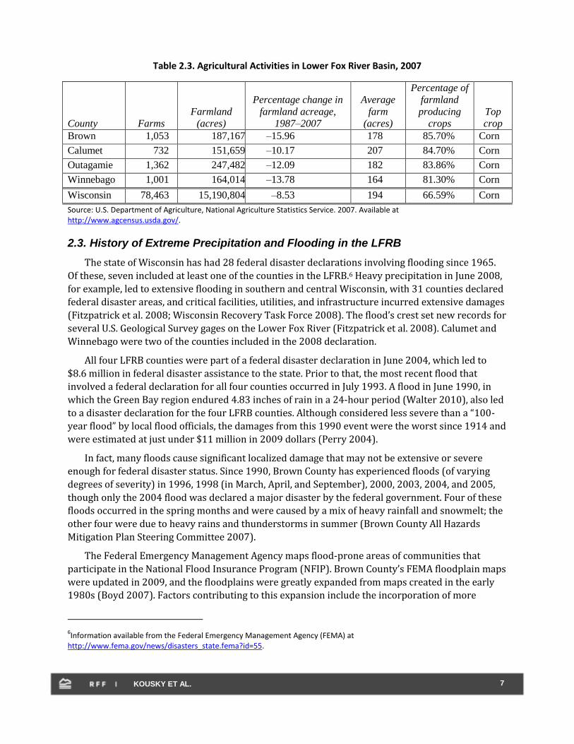
Brown 1,053 187,167 –15.96 178 85.70% Corn

Calumet 732 151,659 –10.17 207 84.70% Corn

Outagamie 1,362 247,482 –12.09 182 83.86% Corn

Winnebago 1,001 164,014 –13.78 164 81.30% Corn

Wisconsin 78,463 15,190,804 –8.53 194 66.59% Corn

Source: U.S. Department of Agriculture, National Agriculture Statistics Service. 2007. Available at http://www.agcensus.usda.gov/.

2.3. History of Extreme Precipitation and Flooding in the LFRB

The state of Wisconsin has had 28 federal disaster declarations involving flooding since 1965.

Of these, seven included at least one of the counties in the LFRB.6 Heavy precipitation in June 2008,

for example, led to extensive flooding in southern and central Wisconsin, with 31 counties declared

federal disaster areas, and critical facilities, utilities, and infrastructure incurred extensive damages

(Fitzpatrick et al. 2008; Wisconsin Recovery Task Force 2008). The flood’s crest set new records for

several U.S. Geological Survey gages on the Lower Fox River (Fitzpatrick et al. 2008). Calumet and

Winnebago were two of the counties included in the 2008 declaration.

All four LFRB counties were part of a federal disaster declaration in June 2004, which led to

$8.6 million in federal disaster assistance to the state. Prior to that, the most recent flood that

involved a federal declaration for all four counties occurred in July 1993. A flood in June 1990, in

which the Green Bay region endured 4.83 inches of rain in a 24-hour period (Walter 2010), also led

to a disaster declaration for the four LFRB counties. Although considered less severe than a “100-

year flood” by local flood officials, the damages from this 1990 event were the worst since 1914 and

were estimated at just under $11 million in 2009 dollars (Perry 2004).

In fact, many floods cause significant localized damage that may not be extensive or severe

enough for federal disaster status. Since 1990, Brown County has experienced floods (of varying

degrees of severity) in 1996, 1998 (in March, April, and September), 2000, 2003, 2004, and 2005,

though only the 2004 flood was declared a major disaster by the federal government. Four of these

floods occurred in the spring months and were caused by a mix of heavy rainfall and snowmelt; the

other four were due to heavy rains and thunderstorms in summer (Brown County All Hazards

Mitigation Plan Steering Committee 2007).

The Federal Emergency Management Agency maps flood-prone areas of communities that

participate in the National Flood Insurance Program (NFIP). Brown County’s FEMA floodplain maps

were updated in 2009, and the floodplains were greatly expanded from maps created in the early

1980s (Boyd 2007). Factors contributing to this expansion include the incorporation of more

6Information available from the Federal Emergency Management Agency (FEMA) at

http://www.fema.gov/news/disasters_state.fema?id=55.

8 KOUSKY ET AL.

accurate topographical data and the addition of major commercial and residential development in

flood-prone areas.7 In addition, FEMA used a model for the impact of Green Bay flooding on river

flows based on new estimates of wave run-up (Boyd 2007). There is controversy among local and

state planners and engineers regarding the accuracy of this new wave run-up model, in addition to

sentiment that the use of even more accurate topographical data (available but not used by FEMA

for the 2009 maps) would have generated different results.8

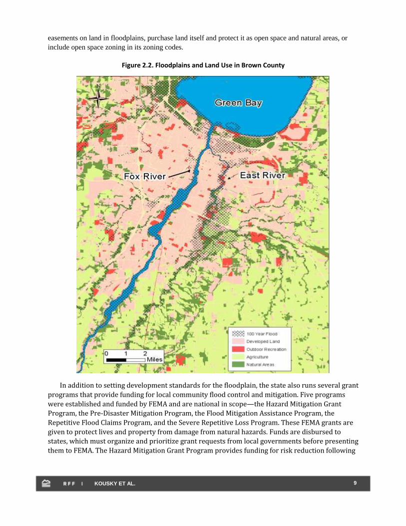
Figure 2.2 shows the updated 100-year floodplains in Brown County, along with accompanying

land uses. The black-hatched areas are the floodplains. In addition to the floodplain near the bay

itself, the map shows a substantial land area in the East River watershed in the 100-year floodplain.

Our overlay of the map with land uses highlights the potential for property damage from flooding,

since the East River floodplain includes a substantial amount of land in developed uses (shown in

beige). We return to the East River watershed issues in Section 2.5.

All cities, villages, and counties in Wisconsin are required to map floodplains and adopt zoning

ordinances that set the rules and requirements governing development in the floodplain. The guidelines

and standards for those ordinances are established in state statutes and administrative code and enforced

by the state’s Department of Natural Resources (DNR).9 State law prohibits many uses in the floodway,

the portion of the floodplain that includes the channel of a river or stream and is associated with moving

water. DNR allows municipalities to issue permits for land uses in these areas that have a relatively low

flood damage potential, such as open space, recreation, agriculture, and parking lots. Most structural

development, however, is prohibited in the floodway. DNR allows only campgrounds, some minimal

structures associated with open space and historical areas, and some structures that are not for habitation,

have low flood damage potential, and/or are functionally dependent on the waterfront.

Most activities and uses are permitted in the flood fringe, the portion of the floodplain that is covered

by standing water during a regional flood but typically not moving water. These uses are subject to

specific development codes and standards, however. Chapter N.R. 116 of the Wisconsin administrative

code requires all residential and commercial structures in the flood fringe to be placed on fill, with the

elevation of the lowest floor of the structure (excluding the basement or crawl space) at least 2 feet above

the regional flood elevation. The fill must be 1 foot or more above the regional flood elevation and extend

at least 15 feet beyond the limits of the structure. The surface of the floor of any basement or crawl space

must be at or above the regional flood elevation. These standards are stricter than the standards that

FEMA requires for communities to participate in the NFIP.10

DNR mandates that all of those standards be incorporated into local subdivision regulations, building

and sanitary codes, flood insurance regulations, and stormwater management regulations where

necessary. In lieu of meeting all the DNR floodplain ordinance requirements, a community can purchase

7 Information provided by Bob Watson, Wisconsin Department of Natural Resources, August 12, 2011.

8 Note that the analysis we perform in Section 4 does not examine coastal flooding from Green Bay, since our focus is on the

East River watershed, where bay flooding is much less of an issue.

9 DNR laws governing floodplains are found in Chapter 87 of the state code; the statutes covering navigable waters and dams

and bridges are Chapters 30 and 31. All chapters are available at http://legis.wisconsin.gov/rsb/Statutes.html. Detailed requirements governing floodplain zoning ordinances and requirements for local communities are in Chapter N.R. 116 of the state administrative code, which is available at https://docs.legis.wisconsin.gov/code/admin_code/nr/116.

10 NFIP floodplain management requirements are discussed on the FEMA website, at

http://www.fema.gov/plan/prevent/floodplain/fm_sg.shtm.

9 KOUSKY ET AL.

easements on land in floodplains, purchase land itself and protect it as open space and natural areas, or

include open space zoning in its zoning codes.

Figure 2.2. Floodplains and Land Use in Brown County

In addition to setting development standards for the floodplain, the state also runs several grant

programs that provide funding for local community flood control and mitigation. Five programs

were established and funded by FEMA and are national in scope—the Hazard Mitigation Grant

Program, the Pre-Disaster Mitigation Program, the Flood Mitigation Assistance Program, the

Repetitive Flood Claims Program, and the Severe Repetitive Loss Program. These FEMA grants are

given to protect lives and property from damage from natural hazards. Funds are disbursed to

states, which must organize and prioritize grant requests from local governments before presenting

them to FEMA. The Hazard Mitigation Grant Program provides funding for risk reduction following

10 KOUSKY ET AL.

a disaster declaration, whereas the Pre-Disaster Mitigation Program offers grants annually. The

goal of the Flood Mitigation Assistance Program is to reduce NFIP claims. The Repetitive Flood

Claims Program and the Severe Repetitive Flood Claims Program are both intended to reduce

repeat claims for NFIP-insured structures.

The state also operates the Municipal Flood Control Grant program, which allows communities

to apply for two types of grants: local assistance grants for administrative activities, and acquisition

and development grants, which can be used to acquire and remove structures in the floodplain,

elevate structures, restore riparian areas, acquire land and easements in the floodplain, and

construct flood control structures. Local communities are required to contribute a minimum 30

percent cost share on each project for the state grants. Grants are awarded every two years with

total funding of approximately $2.5 million to $3.5 million in each round. More than $15 million has

been awarded since 2002. The largest number of grants is for property acquisition and structure

removal projects—approximately half of all funded projects since 2002 fall into this category and

account for slightly more than half of all dollars awarded.11

2.4. Water Quality Problems in the River Basin

There are currently 27 river and stream segments in the LFRB with excessive phosphorus

and/or sediment levels, and these require 45 individual TMDLs under the Clean Water Act

(CADMUS 2010). Between 1993 and 2008 the annual summer median total phosphorus

concentration found at the mouth of the Fox River ranged from 0.12 to 0.28 mg/L, above the 0.1

mg/L target set in the TMDL plan. In the same time frame and sampling station, annual summer

median total suspended solids (TSS) concentrations ranged from 26 to 62 mg/L, exceeding the

TMDL, 18 mg/L (CADMUS 2010). Nutrients and sediment create problems such as eutrophication,

toxic algae blooms, and related reductions in water clarity. These problems can necessitate

swimming advisories and beach closures, diminish the quality of recreation, and harm both

commercial and recreational fishing by contributing to fish mortality. For example, a bloom of

aquatic plants may include toxic blue-green algae, or cyanobacteria, which are harmful to fish and

pose risks to humans. In addition, high levels of phosphorus act as a fertilizer for aquatic plants and

create large areas of excessive vegetation that prevent access to waterways for recreational

activities (CADMUS 2010). These issues are occurring in other areas of the Great Lakes region, and

some studies have estimated that restoration of the lakes would generate large economic benefits

to the region. For example, a 2007 study by the Brookings Institution estimated that a cleanup of

the Great Lakes costing $20 billion would generate more than $50 billion in long-term benefits

(Austin et al. 2007a). The current TMDL plan for the LFRB calls for a 59.2 percent and 54.9 percent

reduction in pounds per year of total phosphorus and TSS, respectively.

Approximately 47 percent of phosphorus loadings in the LFRB are from agriculture (Hafs

2011). Manure from cattle operations is spread on fields and runs off into waterways, leading to

high levels of nitrogen and phosphorus. Although less land is in agriculture in the LFRB now than in

1987 (see Table 2.3), the number of cattle has remained steady as dairy operations have become

concentrated on smaller amounts of land. Thus a relatively constant amount of manure is spread on

fewer acres of land, leading to increasing nutrient loads to area waters. Moreover, to support

concentrated animal feeding operations, farmers have switched from alfalfa and other grasses to

11

Information provided by Jeffrey Soellner, Wisconsin Department of Natural Resources, August 12, 2011.

11 KOUSKY ET AL.

row crops like corn and soybeans, which provide less groundcover in the winter months and

increase runoff from fields in the spring months. Between 1987 and 2007, forage land (land planted

in hay, alfalfa, and grass silage) declined between 77 and 84 percent in the four LFRB counties,

replaced by soybeans and corn (and converted from agriculture to developed uses).

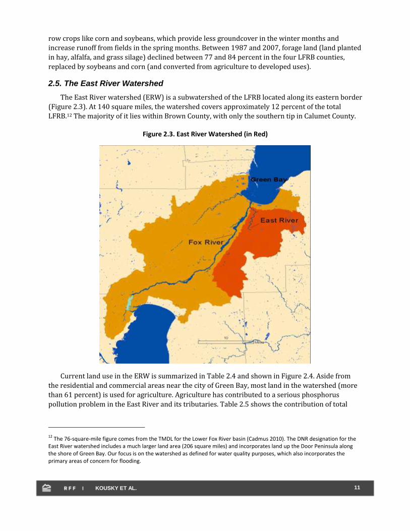
2.5. The East River Watershed

The East River watershed (ERW) is a subwatershed of the LFRB located along its eastern border

(Figure 2.3). At 140 square miles, the watershed covers approximately 12 percent of the total

LFRB.12 The majority of it lies within Brown County, with only the southern tip in Calumet County.

Figure 2.3. East River Watershed (in Red)

Current land use in the ERW is summarized in Table 2.4 and shown in Figure 2.4. Aside from

the residential and commercial areas near the city of Green Bay, most land in the watershed (more

than 61 percent) is used for agriculture. Agriculture has contributed to a serious phosphorus

pollution problem in the East River and its tributaries. Table 2.5 shows the contribution of total

12

The 76-square-mile figure comes from the TMDL for the Lower Fox River basin (Cadmus 2010). The DNR designation for the East River watershed includes a much larger land area (206 square miles) and incorporates land up the Door Peninsula along the shore of Green Bay. Our focus is on the watershed as defined for water quality purposes, which also incorporates the primary areas of concern for flooding.

12 KOUSKY ET AL.

phosphorus in each of the subwatersheds in the LFRB; at 89,000 pounds per year, the ERW has the

highest contribution, except for the Lower Fox River itself.

Table 2.4. Distribution of Land Use in East River Watershed1

Land use Acres Percentage

Agriculture 54,334 60.64

Natural areas 16,138 18.01

Residential 12,220 13.64

Recreation 2,123 2.37

Industrial 1,726 1.93

Commercial 1,293 1.44

Government, institutional 963 1.07

Transportation 422 0.47

Utilities 379 0.42

Total 89,598 100% 1Numbers in this table were calculated using GIS data on land use in Brown County, obtained from the Brown

County Land Planning and Services Department.

Table 2.5. Sources of Total Phosphorus Loads in LFRB, by Subwatershed

Subwatershed Total phosphorus (lbs/yr)

Lower Fox River (main) 237,339

East River* 89,003

Duck Creek 63,172

Apple Creek 35,088

Plum Creek 31,569

Kankapot Creek 20,050

Ashwaubenon Creek 15,681

Dutchman Creek 15,280

Lower Green Bay 12,652

Neenah Slough 11,912

Mud Creek 6,594

Garners Creek 6,575

Trout Creek 4,518

Total (basin) 549,703 Source: Hafs (2011). *Includes Baird and Bower Creek.

A defining feature of the landscape in Brown County and the ERW is the Niagara escarpment,

which forms the eastern boundary of the Fox River valley and rises abruptly 200 to 250 feet above

the valley floor. Several small streams drain down the western side of the escarpment and into the

East River. Associated with the escarpment are karst features—cracked bedrock that lies close to

the ground surface. These cracks are easily dissolved by water and allow pollutants to reach

groundwater. Many shallow soils and sinkholes are in the area (Brown County All Hazards

Mitigation Plan Steering Committee 2007; Hafs 2011). An additional problem is the conversion of

land on the escarpment from natural uses to development. The accompanying impervious surfaces

exacerbate flooding and some pollution problems.

13 KOUSKY ET AL.

Figure 2.4. Land Use in East River Watershed

Currently, more than 10,000 parcels (a parcel is a contiguous plot of land under one ownership)

lie in the 100-year floodplain in Brown County, covering 56,375 acres of land (17 percent of the

county). The improved value of structures on this land was estimated at $1.5 billion in 2007 (Brown

County All Hazards Mitigation Plan Steering Committee 2007). There is a 46 percent projected

increase in residential, commercial, and industrial land uses in the entire county by 2025; the

expected increase in values for floodplain lands is $500,000 (Brown County All Hazards Mitigation

Plan Steering Committee 2007). Much of the increase in development is expected to occur in

communities that have a substantial portion of their land areas in the floodplain. The villages of

Bellevue and Ledgeview, for example, have more than 300 residential parcels in the floodplain,

constituting approximately 68 percent of all parcels in those communities. These are two of the

fastest-growing municipalities in the county. Figure 2.5 shows the land that is in the 100-year flood

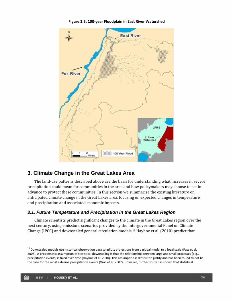
floodplains in the ERW. We say more about future development and flood damages in Section 4.

14 KOUSKY ET AL.

Figure 2.5. 100-year Floodplain in East River Watershed

3. Climate Change in the Great Lakes Area

The land-use patterns described above are the basis for understanding what increases in severe

precipitation could mean for communities in the area and how policymakers may choose to act in

advance to protect these communities. In this section we summarize the existing literature on

anticipated climate change in the Great Lakes area, focusing on expected changes in temperature

and precipitation and associated economic impacts.

3.1. Future Temperature and Precipitation in the Great Lakes Region

Climate scientists predict significant changes to the climate in the Great Lakes region over the

next century, using emissions scenarios provided by the Intergovernmental Panel on Climate

Change (IPCC) and downscaled general circulation models.13 Hayhoe et al. (2010) predict that

13

Downscaled models use historical observation data to adjust projections from a global model to a local scale (Patz et al. 2008). A problematic assumption of statistical downscaling is that the relationship between large and small processes (e.g., precipitation events) is fixed over time (Hayhoe et al. 2010). This assumption is difficult to justify and has been found to not be the case for the most extreme precipitation events (Vrac et al. 2007). However, further study has shown that statistical

15 KOUSKY ET AL.

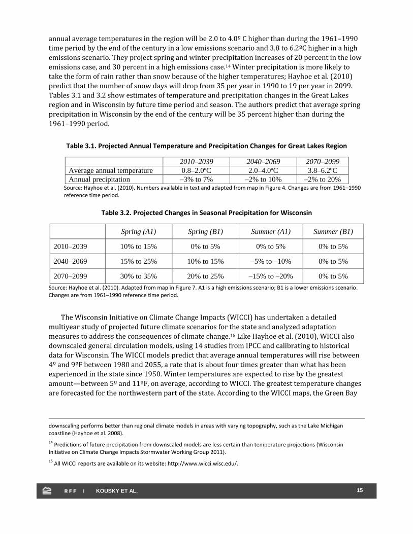
annual average temperatures in the region will be 2.0 to 4.0º C higher than during the 1961–1990

time period by the end of the century in a low emissions scenario and 3.8 to 6.2ºC higher in a high

emissions scenario. They project spring and winter precipitation increases of 20 percent in the low

emissions case, and 30 percent in a high emissions case.14 Winter precipitation is more likely to

take the form of rain rather than snow because of the higher temperatures; Hayhoe et al. (2010)

predict that the number of snow days will drop from 35 per year in 1990 to 19 per year in 2099.

Tables 3.1 and 3.2 show estimates of temperature and precipitation changes in the Great Lakes

region and in Wisconsin by future time period and season. The authors predict that average spring

precipitation in Wisconsin by the end of the century will be 35 percent higher than during the

1961–1990 period.

Table 3.1. Projected Annual Temperature and Precipitation Changes for Great Lakes Region

2010–2039 2040–2069 2070–2099

Average annual temperature 0.8–2.0ºC 2.0–4.0ºC 3.8–6.2ºC

Annual precipitation –3% to 7% –2% to 10% –2% to 20% Source: Hayhoe et al. (2010). Numbers available in text and adapted from map in Figure 4. Changes are from 1961–1990 reference time period.

Table 3.2. Projected Changes in Seasonal Precipitation for Wisconsin

Spring (A1) Spring (B1) Summer (A1) Summer (B1)

2010–2039 10% to 15% 0% to 5% 0% to 5% 0% to 5%

2040–2069 15% to 25% 10% to 15% –5% to –10% 0% to 5%

2070–2099 30% to 35% 20% to 25% –15% to –20% 0% to 5%

Source: Hayhoe et al. (2010). Adapted from map in Figure 7. A1 is a high emissions scenario; B1 is a lower emissions scenario. Changes are from 1961–1990 reference time period.

The Wisconsin Initiative on Climate Change Impacts (WICCI) has undertaken a detailed

multiyear study of projected future climate scenarios for the state and analyzed adaptation

measures to address the consequences of climate change.15 Like Hayhoe et al. (2010), WICCI also

downscaled general circulation models, using 14 studies from IPCC and calibrating to historical

data for Wisconsin. The WICCI models predict that average annual temperatures will rise between

4º and 9ºF between 1980 and 2055, a rate that is about four times greater than what has been

experienced in the state since 1950. Winter temperatures are expected to rise by the greatest

amount—between 5º and 11ºF, on average, according to WICCI. The greatest temperature changes

are forecasted for the northwestern part of the state. According to the WICCI maps, the Green Bay

downscaling performs better than regional climate models in areas with varying topography, such as the Lake Michigan coastline (Hayhoe et al. 2008).

14 Predictions of future precipitation from downscaled models are less certain than temperature projections (Wisconsin

Initiative on Climate Change Impacts Stormwater Working Group 2011).

15 All WICCI reports are available on its website: http://www.wicci.wisc.edu/.

16 KOUSKY ET AL.

area, in northeastern Wisconsin, is expected to see an average temperature increase that is

approximately equal to the average for the state.

Model forecasts of future temperature and precipitation increases are supported by historical

data that show climate change is already taking place in the Great Lakes region and in Wisconsin.

Temperatures in the past three decades have often been above average, with several months

recorded as the hottest on record. The last spring freeze has been occurring earlier, water

temperatures have increased in some locations, periods of ice cover on the lakes have been shorter,

and summer and winter precipitation has been above average for the past three decades (Kling et

al. 2003). Time-series analyses of climate records going back to the beginning of the 20th century

show that air temperatures have been increasing by approximately 0.11ºC per decade in spring and

0.06ºC in winter since 2011 (Magnuson et al. 1997). WICCI has uncovered similar evidence for

Wisconsin: the average annual temperature in the state rose by 1.5ºF between 1950 and 2006

(WICCI 2011). Most of the increase has come in the winter months; the state has experienced a

sharp decline in the number of winter nights below 0ºF. The Green Bay region, for example,

experienced six fewer nights per year below 0ºF in 2006 than in 1950.

Some studies have found that average annual precipitation for the state has risen in recent

decades. WICCI (2011) shows that the average rose 10 percent, or 3.1 inches, between 1950 and

2006, though this has been highly variable across the state. The Green Bay region has seen

precipitation increases slightly below average—between 1.75 and 2.0 inches, according to the

WICCI Stormwater Working Group (2011). That study found no statistically significant increase

over the 1950–2006 period in average annual precipitation totals for three cities—Madison, Green

Bay, and Minneapolis; only Milwaukee saw a significant increase. Studies of precipitation from the

early part of the 20th century show that annual average precipitation in the Great Lakes region as a

whole has increased 2.1 percent per decade since 1911 (Magnuson et al. 1997; Kling et al. 2003).

3.2. Extreme Precipitation in the Great Lakes Region

Most researchers agree that the frequency and severity of extreme precipitation events will

increase in the future. Some evidence suggests that this has already occurred. In a study analyzing

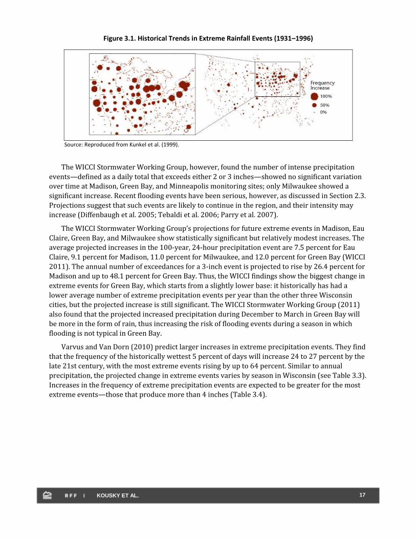
time trends of extreme precipitation events for the United States and Canada, Kunkel et al. (1999)

found that the frequency of extreme precipitation events occurring on average once per year—that

is, “one-year” floods16—has increased 3 percent per decade nationally in the U.S. since the early

part of the century; five-year floods have increased by 4 percent per decade nationally in the U.S.17

The Great Lakes region has accounted for a large portion of this increase, as shown in Figure 3.1,

with frequencies rising over 50 percent (Kunkel et al. 1999). And in Wisconsin, some evidence

suggests a significant increase in extreme precipitation events in recent decades. Angel and Huff

(1997) show that the number of extreme events over the past three decades was twice the number

projected using pre-1957 data.

16

A 1-year flood in this context refers to an extreme precipitation event that has a recurrence interval of 1 year. This classification can be extended to a 5- or 100-year flood based on the severity and probability of its occurring.

17 It is important to note that flooding is not solely related to extreme precipitation.

17 KOUSKY ET AL.

Figure 3.1. Historical Trends in Extreme Rainfall Events (1931–1996)

Source: Reproduced from Kunkel et al. (1999).

The WICCI Stormwater Working Group, however, found the number of intense precipitation

events—defined as a daily total that exceeds either 2 or 3 inches—showed no significant variation

over time at Madison, Green Bay, and Minneapolis monitoring sites; only Milwaukee showed a

significant increase. Recent flooding events have been serious, however, as discussed in Section 2.3.

Projections suggest that such events are likely to continue in the region, and their intensity may

increase (Diffenbaugh et al. 2005; Tebaldi et al. 2006; Parry et al. 2007).

The WICCI Stormwater Working Group’s projections for future extreme events in Madison, Eau

Claire, Green Bay, and Milwaukee show statistically significant but relatively modest increases. The

average projected increases in the 100-year, 24-hour precipitation event are 7.5 percent for Eau

Claire, 9.1 percent for Madison, 11.0 percent for Milwaukee, and 12.0 percent for Green Bay (WICCI

2011). The annual number of exceedances for a 3-inch event is projected to rise by 26.4 percent for

Madison and up to 48.1 percent for Green Bay. Thus, the WICCI findings show the biggest change in

extreme events for Green Bay, which starts from a slightly lower base: it historically has had a

lower average number of extreme precipitation events per year than the other three Wisconsin

cities, but the projected increase is still significant. The WICCI Stormwater Working Group (2011)

also found that the projected increased precipitation during December to March in Green Bay will

be more in the form of rain, thus increasing the risk of flooding events during a season in which

flooding is not typical in Green Bay.

Varvus and Van Dorn (2010) predict larger increases in extreme precipitation events. They find

that the frequency of the historically wettest 5 percent of days will increase 24 to 27 percent by the

late 21st century, with the most extreme events rising by up to 64 percent. Similar to annual

precipitation, the projected change in extreme events varies by season in Wisconsin (see Table 3.3).

Increases in the frequency of extreme precipitation events are expected to be greater for the most

extreme events—those that produce more than 4 inches (Table 3.4).

18 KOUSKY ET AL.

Table 3.3. Projected Change in Frequency of Extreme Precipitation Events for Wisconsin, Late 20th to Late 21st Century

Percentage change

Winter 5 to 41%

Spring 35 to 61

Summer –28 to 60

Autumn –2 to 12

Annual 10 to 40

Source: Patz et al. (2008). Adapted from images showing changes for the Great Lakes region. Extreme precipitation events are defined as the wettest 5% of all days in the late 20th century.

Table 3.4. Projected Change in Frequency of Heavy Precipitation in Wisconsin by Late 21st Century

Rainfall (inches) Percentage change

1 to 1.5 7 to 9.5%

1.5 to 2 10 to 18

2 to 2.5 10 to 18

2.5 to 3 15 to 22

3 to 4 24 to 32

4+ 33 to 63

Source: Patz et al. (2008). Adapted from images showing changes for the Great Lakes region.

3.3. Projected Economic Impacts from Changes in Extreme Precipitation

An increase in the average number of extreme precipitation events and/or an increase in the

severity of events will increase the risk of flooding and the expected damages to buildings and

infrastructure in flood zones. In addition, greater average annual precipitation and more extreme

events will increase the total urban and agricultural runoff into rivers and lakes. Cherkauer and

Sinha (2010) estimate the change in average seasonal runoff volumes in Wisconsin for 2070–2099

due to climate change. These projections are shown in Table 3.5. Most of the increased runoff is

expected in winter and spring because in those seasons, greater precipitation is expected, the soils

are frozen and thus exacerbate runoff, and the precipitation usually coincides with snowmelt (Kling

et al. 2003).

19 KOUSKY ET AL.

Table 3.5. Projected Change in Total Runoff in Wisconsin, 2070–2099

Percentage change

Winter 60 to 90%

Spring 20 to 40

Summer –14 to 21

Autumn –18 to 6

Source: Cherkauer and Sinha (2010). Note: Average seasonal cumulative total runoff (runoff + baseflow) is shown as a percentage change from the base to the late-century period for each of the three scenarios modeled.

Although those projections are far into the future, we can surmise about their link with a

changing climate and illustrate the range of associated problems that could arise, based on

historical experience. More frequent, more extreme precipitation events increase runoff and

flooding, which exacerbate water quality problems. In many areas of the LFRB, and the ERW in

particular, the soils are saturated with phosphorus as a result of decades of agricultural activity.

Flood events lead to a great deal of phosphorus pollution in waterways, which can contribute to

algal blooms and “dead zones”—areas of water depleted of oxygen where marine life cannot be

supported. Many lakes and streams of the Great Lakes region, including the LFRB, have struggled

with dead zones. The earlier springs associated with climate change may also contribute to dead

zones because an earlier spring means a longer period of stratification in lakes, when new oxygen is

not mixing into the water column. In the Great Lakes, mixing usually occurs in the spring and again

in the fall; the deeper lakes, such as Lake Michigan, become stratified in summer (Kling et al. 2003;

Allen and Ingram 2002). Vital Great Lakes species such as the northern pike are especially affected

by these problems.

Another costly result of increased stormwater runoff in past experience—one that illustrates

the breadth of problems that can arise with future extreme precipitation—is the effect on public

health and recreational activity. An example is the closing of public beaches due to bacterial

contamination (Curriero et al. 2001; McLellan et al. 2007). In 2005, the Great Lakes region

experienced a total of 3,000 days of beach closures and advisories, an increase of 4 percent from the

previous year (Austin et al. 2007a). In 2008, Wisconsin alone had 578 closures and advisories (Silva

and McLellan 2010). High levels of Escherichia coli and other potentially harmful pathogens are

most often the cause of a beach closure (McLellan et al. 2007). Potential sources of E. coli

contamination of Wisconsin beaches include urban stormwater, leaky sanitary sewer pipes, sewage

overflows, and agriculture runoff (Silva and McLellan 2010). Contamination from stormwater

runoff reaches public beaches most often during times of high precipitation (Silva and McLellan

2010). Although the city of Green Bay has a storm sewer system that is separate from its sanitary

sewer system, aging water infrastructure can allow sanitary sewer overflow to infiltrate

stormwater pipes and discharge directly into recreational waters (Silva and McLellan 2010). In

addition, wildlife and waterfowl feces contribute to high levels of E. coli in both beach sand and

20 KOUSKY ET AL.

water (Wisconsin DNR 2009).18 In addition to the costs to human health, the reduction in

beachgoers contributes to economic losses in the tourism sector and the overall economic value of

Great Lakes beaches (Austin et al. 2007a).

4. Modeling and Estimating the Economic Costs of Flooding

We turn next to considering the economic costs of flooding, focusing in this section on damage

to property. During the 20th century in the United States, floods were the natural disaster

responsible for the highest amount of property damage (Perry 2000).19 Flooding damages

structures, their contents, infrastructure, and crops. The costs of flooding also include debris clean-

up, the loss of income when businesses must shut down, emergency response costs, and temporary

housing costs for displaced people. Further, flooding can wash sediment and nutrients into waters,

causing pollution problems and associated damages. For instance, it is thought that the 2011

flooding on the Missouri and Mississippi and tributaries may lead to one of the largest recorded

dead zones in the Gulf of Mexico.

We estimate the economic costs of flooding using a model called Hazus-MH, developed by FEMA

and the National Institute of Building Sciences. We describe this model in Section 4.1. We use Hazus

to estimate flood damages in the ERW based on 2010 land-use data and then again for projected

increases in development in roughly 2025 (the year varies for some of the communities in the

county, ranging from 2022 to 2025). These results are presented sequentially. We conclude the

section by discussing who pays for flood damages and the incentives created by the way these flood

costs are distributed.

It is important to note that the estimates of flood damages presented in this report should be

taken only as indicative of magnitude and not as precise predictions. The predominant goal of this

analysis was not to develop accurate flood damage predictions for the ERW but to demonstrate

how Hazus can be used as a planning tool to help local communities at risk for flooding design

policies to mitigate that risk. To this end, the section also includes information for local

governments on how to improve and customize the use of Hazus.

4.1. Estimating Flood Damages with Hazus20

Floods are often discussed in return periods—for example, the 100-year flood event. The 100-

year flood has a 1 in 100, or 1 percent, chance of occurring in any given year. This is equivalent to a

26 percent chance of flooding over the life of a 30-year mortgage. In this study, we focus on four

costs of flooding: damages to structures and contents, damages to crops, damages to infrastructure,

and debris removal. We estimate these damages for 10-year, 50-year, 100-year, and 500-year flood

18

Polychlorinated biphenyls (PCBs) are a significant ecological stressor that historically entered the Green Bay ecosystem through discharge from paper mills (Wenger and Harris 2010). Although they are important regional pollutants, their presence and transport in sediments may be less influenced by climate change than the nutrients and bacteria we discuss here.

19 Floods are also the natural disaster responsible for the most loss of life. We do not focus on loss of life in this analysis since

advanced warning systems and evacuation have dramatically reduced lives lost to flooding, particularly of the sort likely to be experienced in Green Bay. Still, flash flooding and the risk to lives is something local governments need to address in their hazard mitigation plans.

20 We thank Jeff Stone of the Association of State Floodplain Managers for his guidance in our use of Hazus and his comments

on this section of the report. Remaining errors are, of course, our own.

21 KOUSKY ET AL.

events. Estimating damages across multiple flood severity levels gives a better indication of the

possible distribution of losses. The 100-year flood is often used for federal regulatory programs, but

examining losses for other flood levels may be of use to local officials and planners.

We estimate flood damages with Hazus (version MR5, run using ArcGIS 9.3.1, SP1), a national,

GIS-based model developed for FEMA by the National Institute of Building Sciences. Hazus is

designed to be used by local officials and emergency planners to estimate losses from floods,

earthquakes, and hurricanes. For example, Maryland has used Hazus to examine vulnerability to

flooding in Maryland counties (Joyce and Scott 2005). The flood component of Hazus allows

estimation of both coastal and riverine inundation. We focus on riverine inundation when

estimating losses for the ERW. To estimate damages, in brief, Hazus couples a flood hazard analysis

(depth and velocity of inundation) with an analysis of economic losses to estimate physical damage

to structures and contents, vehicles, infrastructure, and agriculture. It also estimates indirect

economic losses and displacement for emergency shelter needs.

To implement the flood hazard module, Hazus relies on a digital elevation model (DEM) to

delineate the stream network for a region. The default DEM for Hazus is from the National Elevation

Dataset maintained by the U.S. Geological Survey (USGS) and has a resolution of 1 arc-second

(about 30 meters). Finer-resolution DEMs can be used instead where available. The level of

resolution for the stream network can be varied from 0.25 to 10 square miles. Finer resolution

allows for evaluation of a more detailed drainage network but requires a trade-off in processing

time (and sometimes, ability of the model to run successfully). Once the stream network is created,

Hazus invokes a hydrology and hydraulics model to generate a flood surface elevation layer for the

study region. For a given return period or discharge volume, this estimates the depth of the flood

from a depth-frequency curve. For more detail on the flood hazard module, see Scawthorn, Blais et

al. (2006).

For the loss module, Hazus draws from national databases of the inventory of structures at the

census block level and for critical facilities at the site-specific level. The data come from the U.S.

Bureau of the Census, and for nonresidential structures, from Dun & Bradstreet. (Users can also

incorporate detailed local-level data on the location and characteristics of structures.) Depth-

damage curves, which link the depth of flooding to the amount of damage to a structure and its

contents, are coupled with the flood surface elevation layer to estimate physical damages. These

vary by occupancy class and building material. Hazus draws on more than 900 depth-damage

curves for structures, their contents, and facilities (Scawthorn, Flores et al. 2006). For each census

block and occupancy class (e.g., residential, commercial, industrial), a damage function is assigned

and, based on the depth of flooding, a percentage of the building is estimated as damaged. This

percentage is then multiplied by the full or depreciated replacement value of that occupancy class.

Hazus also estimates debris generation, indirect losses (such as loss of income or relocation

expenses), and displacement of people. For more information on the loss estimation, see

Scawthorn, Flores et al. (2006).

Hazus can operate at three levels depending on the needs and expertise of the user. A Level 1

analysis uses default data and models. A Level 2 analysis integrates detailed user-supplied data. A

Level 3 analysis requires even more sophistication—such as importing results from third-party

studies and modifying assumed relationships, such as depth-damage curves—but can greatly

improve estimation. In this study, we undertake a Level 2 analysis. We upgrade the DEM to a

22 KOUSKY ET AL.

resolution of 1/3 arc-second (10 meters), from USGS. We also update the building inventory using

local data, as we discuss further in Section 4.2.

As with any model, caution is needed when interpreting Hazus results. The Hazus model makes

simplifying assumptions in the hydrology, hydraulics, and damage estimation modules. For

instance, the damage sustained to a structure depends on its age (because this proxies for building

codes) and its foundation type, which determines the elevation of the first floor. For age, Hazus

assumes a distribution based on Census data. Foundation types are assumed based on whether

homes are in a riverine zone, a lake zone, or the coast. In some instances, more detailed, locally

specific data can improve estimation. In any case, because of these and other assumptions made in

the model, damage and flood depths from Hazus should be taken only as indicative of magnitude

and not as precise predictions.

4.2. Improving Estimation with Hazus

A Level 1 Hazus analysis is designed to be easy for an inexperienced user to run. The software is

free to the public but does require purchase and installation of ArcGIS Desktop software from the

Environmental Systems Research Institute (ESRI). A user manual and a technical manual that can

be downloaded from the FEMA website, and both FEMA and ESRI offer tutorials. Ease of use is the

reason to undertake a Level 1 analysis. Used as a starting point to get a ballpark understanding of

local or regional hazards, it can be helpful to local planners and officials. The drawback is that

estimates may have large error bars from the default assumptions made.

In a Level 2 analysis, users have many options for improving model results. First, they can use a

finer-scale DEM. USGS has higher-resolution DEMs available, or local officials may have their own.

This generally improves the estimation of the stream network. However, the cost is a large increase

in computer processing power and time, and it may not be worth the extra hours of run time to use

the finest-resolution DEM available. Here, we used a 1/3 arc-second DEM, as opposed to the 1 arc-

second default DEM. Even higher-resolution DEMs are available.

Second, users can update the inventory data in Hazus. There are many ways this can be done;

we mention two options using the Comprehensive Data Management System (CDMS). Users can

update either site-specific inventory data (information on particular facilities) or the inventory data

that are aggregated at the census block level. The site-specific inventory data can be used for close

examination of critical facilities, such as hospitals or schools. Users can improve the information on

these places beyond the defaults used in Hazus. Additionally, users can update the aggregated

building counts or exposure data, as we have done in this report. This requires processing tax

assessors’ data (or other parcel-specific data) to match Hazus inventory categories and then

aggregating to the census block level. This can be a time-consuming process, depending on the state

of the parcel data. It may introduce some error as well, since all structures must be slotted into

Hazus categories. Still, it should improve the estimation of building counts and loss estimates. How

much of an improvement will depend on how closely the census data approximate local conditions.

All individual structures can be analyzed without aggregating to the census block level by using the

user-defined facility tools in Hazus; we did not do this, however, because it required either detailed

information on the structures that was not available in Brown County or making assumptions about

their values.

23 KOUSKY ET AL.

In a Level 2 analysis, the user can also improve the hydrology and hydraulics modeling by using

the flood information tool in Hazus. This allows the user to have a floodplain delineated based on

user-supplied data, such as FEMA’s digital flood insurance rate map. The user needs to have a DEM,

flood elevation cross sections, and a floodplain analysis boundary layer. The flood information tool

tool was not used here, however, because it requires one seamless polygon of the floodplain, which

would have taken a large amount of processing time to create (the FEMA data consist of many tiny

polygons).

Several parameters in Hazus can be adjusted by users who have information superior to the

defaults used in the model. The expected debris generated from different types of structures can be

updated based on the depth of flooding, for example. For the shelter and displaced households

analysis, users can specify an evacuation buffer and the percentage of the population assumed to

seek shelter based on demographic factors. For analysis of agricultural damage, users can set the

assumed date of the flood. For business impacts, users can specify annual gross sales per square

foot for different commercial and industrial classes, as well as the estimated time for repair and

parameters governing loss of income and relocation expenses. Finally, more experienced users can

also update information on the assumptions of structure types (foundation material, first-floor

elevation, age) as well as choose (or modify) different default depth-damage curves from among

those available in Hazus.

Local governments will need to trade off the costs of model improvements with the benefits of

improved estimation. This will depend in part on why and how Hazus is being used. If Hazus is

being used to get a broad, general look at potential flood risks, it may not be worth the time to

improve the model. If, however, local officials or planners would like to use Hazus to get better

estimates for flood policy decisions, at least some improvement in the model would be

recommended. Hazus can be difficult to work with when moving beyond a Level 1 analysis, so local

officials should be prepared to spend time learning how to use the model and adapting tabular and

geospatial data. The Hazus support desk provides help on questions that are not answered in the

user and technical manuals.

A final note on using Hazus is that it should be run on a machine with more processing power

than the recommended amount. The flood module is very time consuming to run, and improving

the hardware can make an enormous difference in run time (or ability of the model to run at all).

The next release of Hazus, planned for the fall of 2011, will be 64-bit compatible, which should

improve matters significantly.

4.3. Flood Damages in the East River Watershed

We first estimate damages from 10-year, 50-year, 100-year, and 500-year flood events on the

East River and its tributaries using an updated building inventory based on local 2010 parcel data

from Brown County.21 The methodology for this is discussed in more detail below. The updating

allowed us to improve estimation of economic damages. Although Hazus still performs analysis at

the census block level, thus averaging water depth and damages over each census block, we have

updated the inventory to more accurately reflect the number and value of structures within each

block.

21 We thank Jeff DuMez, GIS Coordinator/Land Information Officer for Brown County, for providing this information.

24 KOUSKY ET AL.

We next updated the building inventory to reflect increased development in the ERW by 2025,

basing the simulated land-use changes on local planning documents. This allowed us to obtain a

rough estimate of flood damages if development were to increase in the watershed, as projected.

For both current and future runs, we used the 1/3 arc-second DEM from USGS. The Hazus user

can specify the size of the drainage area to be used. We chose to create a highly defined stream

network that includes more tributaries by making the size of the drainage area 0.5 square miles. We

set the date of the flood to June 1 (this date is used in estimating agricultural losses).

4.3.1 Damages with 2010 Inventory

To develop more accurate estimates of flood damage, we updated the default inventory in

Hazus using the CDMS22 based on two parcel-level GIS files obtained from Brown County.23 A

parcel-level file of 2010 land use let us match each parcel to the 32 occupancy classes used in

Hazus. Some matches were straightforward, such as single-family dwellings, whereas others were

more complicated and required us to make some assumptions. For instance, Brown County

identified specific utilities and communications structures, such as power substations, landfills, and

pumping stations. We had to map these into a Hazus class, ultimately choosing to label them IND2,

or light industrial. This introduces some errors into the updated inventory, but updating should still

produce a more accurate representation of the building stock in the region than relying on the

default data because the number of structures and exposure at a block level will be more accurate.

We used this land-use file to improve the estimate of the counts of structures in each block.

To improve the estimates of exposure of structures, we used a parcel-level file from the tax

assessor. This gave the assessed value of both land and improvements. The value of improvements

was taken as our estimate of exposure (damages are calculated from this number; Hazus defaults

are estimates of replacement cost). This was then matched to the Hazus land-use categories and

aggregated to the census block level for entry into Hazus using CDMS.24

For a 100-year flood, we compared the results of this updating with results using the Hazus

default inventory. Although updating the inventory theoretically leads to more accurate results, we

found the actual change to be somewhat small. We are aware that there is a false level of precision

in Hazus output numbers, but we report here the model output, while again cautioning the reader

about interpretation. With the default inventory, Hazus estimated that 136 buildings would be

moderately damaged, and with the updated inventory, this jumped to 287 buildings. Estimated total

building-related losses were $85.02 million with the default inventory, versus $83.66 million with

the updated inventory (all values adjusted to 2010 dollars). This is a very small difference, but

other locations might see larger differences, depending on how well the default data characterize

the region. Our update uses assessed values of structures, whereas Hazus default data are estimates

22

ESRI offers an online tutorial on how to accomplish this: http://training.esri.com/gateway/index.cfm?fa=catalog.webCourseDetail&courseid=2073.

23 We thank Jeff DuMez for these files.

24 One complication was that some parcels in the assessor’s data had been subdivided in the land-use file because of different

land uses on one parcel. We thus had to decide, for these parcels, which land-use code to use in Hazus when matching the exposure to an occupancy class. We ultimately decided that for parcels that had a small amount of open space or agriculture and the rest in a higher-valued category, we would use the higher-valued code. For the remaining small number of split parcels, we chose randomly.

25 KOUSKY ET AL.

of replacement cost. Note that the building number count changed dramatically, likely because the

default building count numbers in Hazus are less accurate: for many occupancy categories they are

calculated based on the average square footage of buildings in that class.

Figure 4.1 shows the flood depth grid generated from the 100-year flood on the ERW. Note that

although the Lower Fox River is visible (on the left), the run estimated flooding in the ERW only,

which does not encompass the Lower Fox. Hazus may not reliably identify areas of shallow ponding

during a flood event, and these areas thus might not be showing on this map. For this and other

reasons mentioned above, the map and damage estimates should be taken as an indication of

possible flood depths and damages, not as precise predictions.

Figure 4.1. East River Watershed Flood Depth Grid

We summarize the damage estimates for 10-year, 50-year, 100-year, and 500-year flood events

in Table 4.1, which provides estimates of total building, content, and inventory loss; business

interruption loss; the number of moderately damaged buildings; the truckloads of debris

generated; the number of displaced households; and agricultural losses. These losses all appear to

be larger than the damages sustained in the area during recent floods. For example, 1990 flood

damages were estimated at $11 million (in 2009 dollars). Table 4.1 also shows that, naturally,

losses increase with higher severity flood events, although interestingly, the increase in estimates is

not dramatic for this watershed. This could be because development in the outer reaches of the

26 KOUSKY ET AL.

floodplain is currently rather limited.

Table 4.1. Summary of Damage Estimates for East River and Its Tributaries

10-year

flood

50-year

flood

100-year

flood

500-year

flood

Total building, content, and inventory loss

(million 2010$)

47.48 70.22 83.66 108.88

Business interruption loss1 (million 2010$) 1.05 1.19 1.30 1.50

Moderately damaged2 buildings 113 236 287 406

Truckloads of debris generated (25 tons each) 74 110 129 173

Displaced households3 2,811 3,201 3,439 3,827

Direct economic loss for agricultural products

(million 2010$)4

4.62 5.54 5.84 6.27

1 This includes relocation costs, income loss, rental income loss, and wage loss.

2 Hazus defines “moderately damaged” as a structure that is 10% to 50% damaged.

3 These numbers are quite high across all runs and we have less faith in them. Hazus estimates more displaced households than

damaged homes because it counts homes that are cut off by flooded roadways and households displaced by a warning. 4 Estimates listed here are based on a three-day flood; agricultural losses depend on duration of inundation.

Table 4.2 breaks down building damages by residential, commercial, industrial, and other

categories. This distribution will be influenced by the choices we made with the 2010 data when

mapping land uses to Hazus categories. The greatest damages are sustained by commercial

structures, quite possibly because they are higher value than residential structures and there is less

industrial development. This is also, obviously, a function of the type of development in the

floodplain. Table 4.3 provides business interruption losses for each category for the 100-year flood,

as an example of the distribution of losses across types of damage. Figure 4.2 shows the flood depth

grid from the 100-year run overlaid with 2010 land use categories.

Table 4.2. Building Loss by Type of Building (million 2010$) for East River and Its Tributaries

10-year flood 50-year flood 100-year

flood

500-year

flood

Residential 15.14 23.43 27.97 37.71

Commercial 26.91 37.61 44.17 55.07

Industrial 5.35 9.06 11.41 15.95

Other 0.08 0.11 0.12 0.15

Table 4.3. Business Interruption Loss by Type of Building for 100-year Flood (million 2010$)

for East River and Its Tributaries

Income Relocation Rental

Income

Wage

Residential 0.00 0.11 0.02 0.00

Commercial 0.24 0.04 0.02 0.27

Industrial 0.00 0.00 0.00 0.00

Other 0.02 0.00 0.00 0.58

27 KOUSKY ET AL.

Figure 4.2. East River Watershed Flood Depth and 2010 Land Use

To show how losses vary spatially across the watershed, Figure 4.3 maps total building related

losses by census block for the 100-year flood. The areas of greatest damage occur where flooding is

deeper and more extensive and structures are more numerous. In all the Hazus runs for the ERW,

two schools have at least moderate damage. There are no losses to major transportation

infrastructure, utilities, or hospitals.

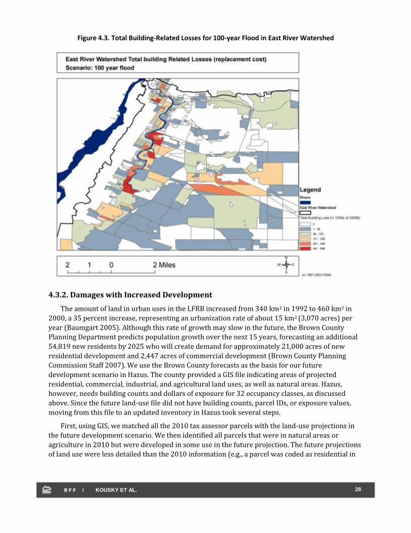
28 KOUSKY ET AL.

Figure 4.3. Total Building-Related Losses for 100-year Flood in East River Watershed

4.3.2. Damages with Increased Development

The amount of land in urban uses in the LFRB increased from 340 km2 in 1992 to 460 km2 in

2000, a 35 percent increase, representing an urbanization rate of about 15 km2 (3,070 acres) per

year (Baumgart 2005). Although this rate of growth may slow in the future, the Brown County

Planning Department predicts population growth over the next 15 years, forecasting an additional

54,819 new residents by 2025 who will create demand for approximately 21,000 acres of new

residential development and 2,447 acres of commercial development (Brown County Planning

Commission Staff 2007). We use the Brown County forecasts as the basis for our future

development scenario in Hazus. The county provided a GIS file indicating areas of projected

residential, commercial, industrial, and agricultural land uses, as well as natural areas. Hazus,

however, needs building counts and dollars of exposure for 32 occupancy classes, as discussed

above. Since the future land-use file did not have building counts, parcel IDs, or exposure values,

moving from this file to an updated inventory in Hazus took several steps.

First, using GIS, we matched all the 2010 tax assessor parcels with the land-use projections in

the future development scenario. We then identified all parcels that were in natural areas or

agriculture in 2010 but were developed in some use in the future projection. The future projections

of land use were less detailed than the 2010 information (e.g., a parcel was coded as residential in

29 KOUSKY ET AL.

2025, but whether it was a single-family home, a condominium, or a duplex was unknown). Based

on the predominant land uses in the county, we made assumptions about what Hazus code would

be used for all parcels that became developed. They were then each assigned the mean value of that

class in the watershed from the 2010 assessor’s information. From this, counts and values were

aggregated to the census block level, and the Hazus inventory was updated using CDMS. Ultimately,

our scenario shows approximately 22,000 additional acres of development, slightly less than the

county’s forecasts.

The biggest drawback of using Hazus for this type of future analysis is that the hydrology does

not update if impervious surface area changes. So our future development scenario runs presented

here for the ERW are based on increased damages from building in floodprone areas. If the

development also increases runoff and flood risk outside the current floodplain, or increases the

flood depth within the current floodplain, the associated damage is not captured in our estimates.

Thus, the change in damages from 2010 to our future scenario is an underestimate. We discuss this

more in Section 6.

Table 4.4 shows a summary of costs for the loss categories of total building loss, business

interruption loss, number of moderately damaged buildings, truckloads of debris, and number of

displaced households with the new development.25 Building losses have increased, depending on

the event, by roughly $8 million to $13 million.

Table 4.4. Summary of Developed Scenario Damage Estimates for East River and Its Tributaries

10-year flood 50-year

flood

100-year

flood

500-year

flood

Total building, content, and inventory loss

(million 2010 $)

55.88 80.11 95.62 123.78

Business interruption loss1 (million 2010 $) 1.05 1.19 1.31 1.50

Moderately damaged2 buildings 122 261 317 434

Truckloads of debris generated (25

tons/truck)

74 110 129 172

Displaced households3 2,811 3,201 3,439 3,827

1 This includes relocation costs, income loss, rental income loss, and wage loss.

2 Hazus defines “moderately damaged” as a structure that is 10% to 50% damaged.

3 These numbers are quite high across all runs and we have little faith in them. Hazus estimates more displaced households

than damaged homes because it counts homes that are cut off by flooded roadways and households displaced by a warning. 4

Estimates listed here are based on a three-day flood; agricultural losses depend on duration of inundation.

For all runs, two schools sustain moderate damage. For the 10-year flood, only one school has

loss of use, but for the 50-year, 100-year, and 500-year floods, both schools face loss of use. No

other critical facilities are damaged.

The increase in flood damages from development in the ERW is not trivial. Other research has

found that development will increase flood risk, particularly in the near term, much more than

climate change. Still, as discussed earlier, changes in climate will alter the hydrology in Brown

County, potentially leading to increases in flooding. With climate change, the 100-year flood of

25

We did not run estimates of future agricultural losses because it required making assumptions about how acreage change from agriculture would link to yields, by crop, within in the entire county. This was beyond the scope of our study.

30 KOUSKY ET AL.

today could be the 50-year flood of tomorrow. Thus, our estimates of damage in the current land-

use scenario may be underestimates of the damage that this area will see. In the subsequent

sections of this report we focus on land-use options for mitigating increases in flood risk. Such

approaches can add resiliency to a community, helping them be “climate-ready” for a wider range of

climate futures than is possible using gray infrastructure.

4.4. Who Pays for Flood Damage?

The costs of flood damage are distributed among individuals, businesses, and all levels of

government. Research reported in Shabman et al. (2011) looked closely at federal payments for

flood damage, and this section draws heavily from that analysis. The incentive communities and

residents have to mitigate flood damages depends, in part, on what fraction of the costs of flood

damage they bear. Theoretically at least, when the costs of a flood are not borne fully by those

making mitigation decisions, inefficient outcomes can result. We look in this section at how the

damages estimated by Hazus are distributed among individuals, businesses, the local government,

the state, and the federal government.

For minor flooding, government bears a smaller portion of the cost than for large flood events.

This is because for large disasters, the president can make a disaster or emergency declaration,

which frees federal relief dollars. (Disasters and emergencies are declared by the president after a

request by a governor and a recommendation from FEMA.) For emergencies, the federal response is

limited to immediate and short-term assistance. Expenditures by FEMA may not exceed $5 million

(GAO 2001), but there is no spending limit for disaster declarations. Once approved, FEMA

distributes money from the Disaster Relief Fund. Each year, funds are appropriated into the

account, where they remain until spent. Congress must pass supplemental legislation for

catastrophes that require more aid than is in the fund. In addition to FEMA, the U.S. Department of

Housing and Urban Development (HUD) and other agencies also offer relief funds following a

presidential disaster declaration and require congressional appropriation of funds.

Whether a disaster declaration is made, therefore, determines whether the federal government

will bear much of the costs of a flood event. It is difficult to say whether flood events in the ERW

would be substantial enough to trigger a disaster declaration, as there are currently no

requirements for a declaration. The Stafford Act requires that for a declaration, a disaster must be

judged to exceed state and local capacity to respond. The act also, however, specifically prohibits

allocating funding based on “an arithmetic formula or sliding scale based on income or population.”

To find a middle ground, in 1999, FEMA published criteria it would use in recommending a

declaration. To determine whether a disaster exceeds state capacity, FEMA considers per capita

damages and total statewide damages from the preliminary assessment. In 1999, it set a trigger of

$1 for the former, to be adjusted for inflation annually, and $1 million for the latter, but not adjusted

for inflation (GAO 2001). These are low thresholds, giving the president considerable discretion in

making a declaration.

Beyond those financial measures, FEMA considers five other criteria before issuing its

recommendation to the president.26 First is the concentration of damages at a local level, since

severe local impacts may warrant federal aid even if the statewide per capital damage trigger is not

met. Second, FEMA reduces the amount of anticipated assistance if there is more insurance in force

26

64 Fed. Reg. 169 (1 September 1999).

31 KOUSKY ET AL.

in a state (or if should have been more in-force insurance, based on current laws and regulations).

Third, if a state has adopted mitigation efforts, such as a building code, FEMA is more likely to grant

assistance even if damages fall below the triggers above. Fourth, FEMA considers whether the state

has recently had to cope with other disasters. And finally, FEMA examines whether relief from other

federal agencies, such as the Department of Agriculture or Federal Highway Administration, would

be more appropriate.

Once the president makes a declaration, FEMA decides how much money to give to states,

counties, and other eligible entities. Not all counties are eligible for assistance when a state receives

a declaration. FEMA provides money through three channels: (1) the Public Assistance Grant

Program, which aids state, local, and tribal governments; (2) individual assistance, which could be

for housing (rental or rebuilding), crisis counseling, unemployment compensation, or other aid to

victims for expenses not covered by insurance or Small Business Administration loans; and (3) the

Hazard Mitigation Grant Program, which gives extra funding to states that help communities

implement measures to reduce future damages (GAO 2001).

Following a declaration, Congress may also direct funding to community development block

grants (CDBG) administered by HUD. Communities can use these funds for a range of rebuilding

and reconstruction costs or cleanup costs not covered by FEMA. In at least two instances

(Hurricane Katrina and the September 11 attacks), HUD allowed states to use CDBG funds to direct

grant programs to individuals (Shabman et al. 2011). Generally speaking, however, this money is

for local governments and not individuals and will be treated as such here.

A final source of aid is Small Business Administration (SBA) loans for rebuilding. These are

provided to individuals or businesses in a disaster declaration area. The loans have a lower interest

rate and longer terms than loans from private financial institutions. Of note, SBA will not lend to

property owners who were required to have flood insurance but did not. The loans are not

available for upgrades beyond what is required by building codes and are capped at $200,000 for

primary residences and $2 million for businesses.

It seems likely that a declaration would be made for 100-year and 500-year flood events along

the East River and tributaries, since if the East River is flooding, nearby rivers are also likely to

flood. Here, we will examine damages from the 100-year flood event as estimated by Hazus with

current 2010 inventory along the East River and its tributaries and discuss who would pay these

damages, either with or without a disaster declaration.

Many federal funds are funneled through the state to local governments. Often the state plays a

role in prioritizing projects for funding and in allocating dollars to localities. Wisconsin also will use

state funds toward relief from flood disasters. The Wisconsin Department of Transportation has a

program to help local governments pay for damaged roads. The state’ Disaster Recovery Fund

issues money to local governments when the county or the state is denied a federal disaster

declaration.

4.4.1. Costs Borne by Homeowners

In the 100-year run for the East River and its tributaries, 195 residential buildings are

estimated to sustain $15.55 million in losses and residential contents another $12.42 million.

Although not all structures will sustain the same amount of damage (indeed, Hazus breaks down

the building losses by percentage damaged), to simplify things, we assume that all homes sustain

32 KOUSKY ET AL.

equal damage, so there is roughly $80,000 damage to each home and $63,700 contents damage to

each household. The various entities that cover some of these residential losses will be discussed in

turn.

First, Brown County participates in the National Flood Insurance Program. This federal

program offers flood insurance to homeowners and businesses in participating communities. For

individuals, the NFIP offers building coverage up to $250,000 and contents coverage up to

$100,000. For homeowners who have purchased the coverage, damages up to coverage limits are

reimbursed. Average annual premium rates (available on the FloodSmart website) can vary from a

few hundred dollars for low-risk homes to several thousand for high-risk homes. Since damages for

the 100-year flood are predicted to be less than the maximum amount of coverage available, if most

homeowners completely insured their houses and contents through the NFIP, they would be fully

reimbursed for the damage. As discussed below in Section 5.2, however, take-up rates for flood

insurance are quite low in Brown County.

If there is no disaster declaration, the only other aid available to homeowners is the ability to

deduct uninsured disaster losses from federal income taxes. Individuals may deduct damages to

their home, household items, and vehicles. The amount must be reduced by any salvage value,

insurance payment, or other aid received.

If a disaster declaration is made, individuals could be eligible for aid from FEMA’s Individual

and Households Program. This is either housing assistance or “other needs assistance.” The former

can be used for repair and rebuilding or to cover costs of temporary housing. The latter can be used

for replacing personal property, transportation, medical costs, or funeral expenses. States must

match 25 percent of the funds, and grants are limited to $30,200 in 2011 (this limit is adjusted

annually for inflation) per person or household. The average grant, however, is only $5,000.

Whereas homeowners must pay premiums for the NFIP insurance, FEMA aid is a cost-free grant to

cover damages, but in a 100-year flood, it would cover only a fraction of the total damages a

household sustained. Homeowners could also receive an SBA loan for primary residences; the

benefit to them is the difference in the interest rate between an SBA loan and a conventional loan.

Individuals can thus receive tens of thousands of dollars in grant money from the federal

government, but for substantial damage, this would be insufficient to make them whole. That said,

riverine flooding on small streams or runoff flooding will not damage a house to the same extent as

full submergence. So for homeowners who face a risk of some damage but are unlikely to suffer a

total loss, federal grants may provide a disincentive to locate out of harm’s way or a disincentive to

adopt risk-reduction measures. That said, in the 100-year flood estimates here, on average damage

is more than double what FEMA would pay, and homeowners would bear these costs.

4.4.2. Costs Borne by Businesses

In the 100-year run with the 2010 updated inventory, commercial structures are estimated to

sustain $13.59 million in damages. Commercial damage to contents is estimated at $29.87 million

and commercial damage to inventory is estimated at $0.70 million. The corresponding three

damage estimates for industrial facilities are $1.85 million, $8.13 million, and $1.43 million. In

addition to this direct damage, commercial institutions are estimated to sustain $0.24 million in

income losses, $0.04 million in relocation expenses, $0.02 million in lost rental income, and $0.27 in

lost wages. Industrial facilities did not experience these losses.

33 KOUSKY ET AL.

Businesses willing to pay the premiums can insure both buildings and contents for up to

$500,000 each through the NFIP. Businesses with exposure beyond the NFIP limits may purchase

private insurance covering the remaining amount. Some businesses, particularly large or diversified

companies, may choose to self-insure against flood risk. Businesses are generally not eligible for

FEMA grants. They may, however, apply for SBA loans with reduced interest rates. Loans are

available for both physical damage and economic injury.

Businesses are eligible for less direct aid than individuals. They likely have either insured

themselves (and thus paid premiums in advance for the claims payouts at the time of the event) or

will take out an SBA or conventional loan to cover damages ex post. The lower rates on SBA loans

represent a small subsidy to businesses hit by a disaster, but, absent empirical investigation into

this issue, the subsidy does not appear to be large enough to significantly alter incentives about

where to locate or whether to invest in risk reduction measures.

4.4.3. Costs Borne by Local Governments

Local governments may sustain damage to buildings or other public infrastructure in a flood

event. In the 100-year run for the ERW, two schools sustained at least moderate damage that would

need to be repaired. The local government would also pay for debris removal. The 100-year flood

run estimated 129 truckloads of debris would need to be cleared. Finally, local governments

provide shelter for displaced people. We believe the Hazus estimates of displaced people are likely

to be overestimates. Regardless, Hazus does not offer estimates of the costs to a local government of

providing shelter.

Local governments can insure their buildings through the NFIP or with a private insurance

company. If the buildings that were damaged had an insurance policy, the government would

receive the claim payment. In addition, communities can receive FEMA grants (passed through the

state) for costs in seven categories: debris removal, emergency protective measures, roads and

bridges, water control facilities, building and equipment, utilities, and parks, recreational facilities,

and other items. There is a 25 percent matching requirement, but the president can waive it. How

this cost-share is split between the state and the community is determined by the state. FEMA will

not provide funds for structures that could have been insured under the NFIP but were not.

Communities may also receive CDBG funds to fill in gaps in relief costs not covered by FEMA.

Damages not covered by the federal government may be covered by the state. Wisconsin has

funds to help rebuild roadways, as mentioned above, and a fund for local governments when a

disaster declaration is not made. If a per capita threshold of damages is met, the community can

apply to the administrator of Wisconsin Emergency Management for funds. Locals must pay a 30

percent cost-share, and the funds can be used to clear debris, institute emergency protective

measures, and rebuild roads.

In short, communities are likely to cover the majority of public flood costs through federal or

state funding. Taxpayers across the state or country are thus covering some of the flood damages

even when they do not choose to reside in a hazard-prone area. This subsidization of local

government costs may discourage the local government from taking protective measures for their

own buildings or infrastructure.

34 KOUSKY ET AL.

5. Policy Options Other Than Land Use for Reducing Flood Damages

This study focuses on land-use changes to mitigate flood damages. There are, however, several

other approaches that can address flood-related costs. We briefly discuss several such options here.

Section 6 provides an overview of the land-use options that can be used to mitigate flood damages.

As this section elucidates, we focus on land-use changes because land-use policies are usually well

within a local government’s control, they can be more affordable than gray infrastructure, they can

produce many co-benefits of concern to local governments, and they can be extremely effective in

lowering flood damages.

5.1. Structural Flood Control

Historically, the predominant approach to flood control in the United States has been the use of

engineered structures, such as levees, floodwalls, and dams. Structural methods of flood control

date back to the earliest settlements along U.S. rivers. With legislation in 1928 and 1936, however,

flood protection became a policy of the federal government. Over the decades, the Corps of

Engineers has overseen the construction of miles of levees, flood walls, dams, and other forms of

gray infrastructure to protect many communities from rising waters.

Structural flood control projects are not cheap, however. Despite a common perception that the

Corps continues to construct massive flood control projects, the reality today is quite different. The

Corps has a huge backlog of flood control projects and a smaller budget than in decades past,

making new federally funded structural flood control projects much less likely (Shabman et al.

2011). In addition, structural flood protection requires periodic maintenance, which the local

government may not have the budget to cover, and for which federal funds may be hard to obtain. If

structural protection is not maintained, over time it may fail to provide the level of protection it was

designed for, increasing the flood risk for unsuspecting local residents.

Research also suggests that flood control construction can impose costs on communities across

the river and communities downstream. Levees hold back waters up to a certain level flood,

protecting those located behind them, but in so doing, they increase flood stages upstream,

accelerate the flow of water downstream, and push water onto neighboring communities. Data on

flood volume and stages for the Missouri and Mississippi rivers show that flood stages have

increased for large discharges of water, most likely because of the construction of engineering

works along the rivers (Belt 1975; Criss and Shock 2001; Pinter and Heine 2002). That is, for a

given amount of water now, the river will rise higher than it would have before the structural flood

control was in place. Land-use changes to control flooding do not create these types of external

costs.27

5.2. Insurance

Flood insurance is available to homeowners and businesses through the National Flood

Insurance Program, as already mentioned. Flooding is usually not a covered peril under

homeowners insurance policies. Indeed, the NFIP was created in 1968 partly in response to the lack

of availability of flood insurance in the private market. The program is designed to be a partnership

27

If the land-use policies decrease the amount of development, it will lower the tax base for a local government. If the development is simply directed away from the floodplain, however, this would not be the case. This is discussed further below.

35 KOUSKY ET AL.

between communities and the federal government. When a community joins the program, it must

adopt minimum floodplain regulations, and in return, flood insurance becomes available to

residents. As we noted already in Section 4, the NFIP offers up to $250,000 coverage for homes and

$100,000 for contents for residential structures, and $500,000 each of building and contents

coverage to businesses.

Flood insurance can help reduce recovery times, spur rebuilding, and limit total property losses

in the event of a flood. For their yearly premiums, homeowners and businesses can have their

covered losses reimbursed after a flood. Despite this benefit, take-up rates for flood insurance have

been quite low in many at-risk areas, spurring Congress in 1973 to adopt a mandatory purchase

requirement that makes flood insurance mandatory for homeowners in 100-year floodplains with

loans from a federally backed or regulated lender. Further, to be eligible for disaster assistance, the

1973 law requires communities to participate in the NFIP.

In 2008 there were 1,613 NFIP policies-in-force in Brown County, and 1,401 of these were in

FEMA-designated 100-year floodplains.28 The Census Bureau estimates there are just over 96,000

households in the county, giving a total take-up rate of about 1.6 percent. The land-use file we

received from Brown County indicates that there are approximately 14,500 parcels that intersect

the FEMA 100-year floodplains, giving a take-up rate in the floodplain of just under 10 percent. In

any event, take-up rates appear to be quite low, and flood insurance will thus likely play only a

limited role in Brown County during significant flood events. Encouraging more widespread

adoption may be socially desirable.

Insurance could also be viewed as a complement to and not a substitute for other mitigation

measures. Cost-effective mitigation measures could be adopted and any residual risk then covered

by insurance, presumably at lower rates reflecting the lower risk.

5.3. Building Regulations

Building regulations can be adopted to reduce damages when a flood occurs. Flood damages

depend on the height of the floodwaters relative to the structure, so common floodplain regulations

include minimum requirements for the ratio of building height to the base-flood elevation. Various

flood-proofing techniques can also be adopted to retrofit structures to reduce potential flood

damages. Some of these activities may be required by local or state law; homeowners may find

adoption of some of them cost-effective and do so voluntarily. Regulations in Brown County were

discussed in Section 2.

The NFIP also requires that buildings be subject to certain regulations. The consequence for

damages can be seen by comparing estimated damages to buildings built before the community

joined the NFIP and those built after, when building codes were in effect. This is estimated in all

Hazus runs. When a community joins the NFIP, a flood insurance rate map (FIRM) is created;

structures before this time are referred to as pre-FIRM, and those after are called post-FIRM. For all

flood events with the 2010 inventory, Hazus estimates less damage to structures that are post-FIRM

compared with those pre-FIRM.

28

We thank Tim Scoville and Erwann Michel-Kerjan for these data.

36 KOUSKY ET AL.

5.4. Warnings and Evacuation

There are many types of floods, from shallow stormwater runoff, to flash floods in narrow

canyons, to slowly rising floods on large river systems. The ability to detect and issue early

warnings varies somewhat for each type, but for the most part, the United States has an effective

system of detection and warning that can be used to evacuate residents in advance of inundation.

Early warning and evacuation save lives and can reduce damage to property that is readily moved,

such as vehicles, and a small amount of personal possessions. Although such systems are critical to

avoid loss of life, they are of limited value in reducing damage to structures. Warning and

evacuation should thus be undertaken in conjunction with other risk reduction measures.

6. Land-Use Options for Mitigating Flood Damage

Converting land to open space or preserving open space can reduce flood damages in three

ways, each of which will be discussed briefly here. First, restoring or preserving wetlands can lower

flood damages because wetlands can act as a natural sponge, absorbing floodwaters. Second, water

can be stored in the soil column, so increasing greenways can allow some water to infiltrate into the

ground, reducing runoff. Finally, if all structures and other assets are removed from an area, then if

the land floods, there is nothing to be damaged. This latter effect of reducing exposure is all that can

be modeled in Hazus. We mention the other benefits of open space in lowering flood damages,

however, because they may be important for local communities when choosing “green” approaches

to flood control.

6.1. Wetlands as Reservoirs

Wetlands can act as natural reservoirs. They store floodwaters and then slowly release them,

delaying and attenuating peak flood flows. There are several examples around the country where

wetlands have been preserved or restored for this purpose. For instance, along the Charles River in

Massachusetts, wetlands were acquired by the Corps of Engineers several decades ago for their

ability to mitigate flooding.

Estimating the flood storage potential of restored wetlands requires hydrologic simulation

(Potter 1994), for which local governments would have to hire outside experts. Still, some rules of

thumb have emerged from modeling studies to date. Perhaps obviously, flood attenuation increases

as wetland area in the watershed increases. Less intuitively, with wetland areas of only 5 to 10

percent, peak flows can be reduced by 50 percent compared with the case of no wetlands (De Laney

1995).

Since wetlands drain slowly, at the time of any given storm, their full storage potential may not

be available; this is especially important for large, regional floods of long duration (Potter 1994).

Because of this, wetlands are most likely to be effective in mitigating the effects of smaller floods

and may not substantially attenuate peaks for very large flood events. For small and medium-sized

floods, however, land cover can have a significant effect (Change and Franczyk 2008).

There is conflicting evidence on whether wetlands are more effective at reducing flood peaks if

scattered in the upper reaches of the watershed or if consolidated downstream. A community

trying to optimize the flood mitigation role of wetlands would need to undertake advanced

modeling for the specific watershed.

37 KOUSKY ET AL.

6.2. Pervious Surface Area and Infiltration

During and after a storm, water can be stored in the soil column. When the ground is compacted

or covered with impervious surface, this storage potential is lost. Precipitation then washes much

more quickly into stream channels, potentially increasing flood peaks and discharge volumes

(Booth et al. 2002). When carefully constructed and located, green areas that mimic natural

hydrology can increase infiltration and slow runoff. Such greenways are often referred to as green

infrastructure and include rain gardens, detention basins, and bioswales, as well as the wetlands

discussed in Section 6.1. Green infrastructure can also reduce pollutant loadings, recharge

groundwater, and increase wildlife habitat, among other benefits. A review of studies of green

infrastructure found them as effective, on average, as conventional infrastructure at reducing water

pollution and also found them to be effective in reducing stormwater peaks and runoff volumes

(Jaffee et al. 2010).

Most research to date has found that green infrastructure is best suited to managing “average”

levels of stormwater. Extreme precipitation events may overwhelm such systems. In areas at risk of

flooding from storm runoff, however, green infrastructure approaches can prove useful. A review

found that green infrastructure could reduce peak flow by 50 percent or more, although sites and

storm events were limited (Jaffee et al. 2010).

In addition to actual land-use change, changes in land management practices could improve

flood control. Manale (2000) has proposed voluntary, targeted payments to landowners to plug

drainage ditches and tile drains so that agricultural land can store more floodwaters. One example

of this type of system has been developed for storing water and sequestering nutrients on

rangelands in Florida (Bohlen et al. 2009).

6.3. Reducing Exposure

During a flood, water overflows stream banks into the surrounding floodplain, damaging

structures located in these areas. Removing structures reduces exposure and thus lowers damage

when a flood occurs. Conversely, increasing exposure in floodplains can increase damages. This was

modeled for the ERW using Hazus in Section 4. Further, if there are natural areas surrounding

rivers into which water can spread, flood heights downstream will be lower than where the river

channel is leveed and water is pushed up and down the river. Whether and where floodplain

development should occur requires weighing the benefits of the development against the expected

costs of flood damage. We turn to this next.

7. Comparing the Benefits of Flood Damage Mitigation with the Costs

In this section, we present a framework for analyzing the benefits and costs of land

conservation in the floodplain as a means of mitigating the damages from flooding. We present

benefit and cost estimates for four alternative scenarios for targeting land parcels for preservation.

We take as our starting point a comparison of expected flood damages in the future, when more

land in the watershed is in developed uses, with expected damages under today’s development

patterns. If the lands that the county projects to be developed are instead protected as natural areas

or remain in agricultural use, flood damages will be lower. These avoided damages are our

estimates of the flood benefits of land conservation. The government can purchase land and retain

it as publicly owned and managed open space or parkland, or it can purchase easements that keep

38 KOUSKY ET AL.

the land in private ownership but restrict development. With agricultural easements, some farming

activity can continue on the land. We discuss and assess the costs of both options.

Finally and importantly, the costs of this approach vary dramatically depending on how parcels

are targeted for preservation. We present a baseline scenario in which all parcels in the floodplain

projected to be developed in the future land-use scenario are instead preserved. We then compare

the costs of that approach (with either fee simple purchase or an easement) with the costs of three

alternative scenarios that more carefully target a subset of parcels. Our scenarios are chosen based

on logic and common sense, and they focus exclusively on flooding concerns. Many experts,

including several environmental economists, have written on the subject of targeting land

conservation for ecosystem services. We discuss that literature and describe how it could be put to

use in our context in Section 7.3.

Our calculations in this section are not meant to be a definitive benefit-cost calculation for the

ERW. Rather, they are illustrative of the way in which such an analysis could be carried out, how the

Hazus model can be used to estimate the benefits of reduced flooding, and how to go about

evaluating the merits of various land conservation options in the floodplain. Targeting parcels is

critical for both maximizing benefits and minimizing costs. Our scenarios shed some light on this

issue, but much work could be done to further refine the approach. We say more about this in

Section 7.3. Finally, the co-benefits of land conservation in the floodplain—most importantly, water

quality improvements and recreational benefits—may be large and even dwarf the flood benefits.

We do not include such co-benefits here in any formal way but discuss them at length in Section 8.

They would need to be considered in any complete benefit-cost analysis.

7.1. The Benefits of Avoided Flood Damages

Although flood magnitudes are often discussed in terms of return intervals—such as the 100-

year flood or the 50-year flood—to evaluate policy options for reducing flood risk, local officials

need some assessment of the annual risk. Expected flood damage in any given year is a more

intuitive number and easier to compare with the costs of policy alternatives than simply projected

damages for a single flood of a given magnitude (return interval). The expected annual damages,

often referred to as the average annualized loss (AAL), is the sum of the probability that a flood of a

certain magnitude will occur, multiplied by the damages if it does. We calculate this number for

both the 2010 land-use scenario and the future developed scenario that we examined in Section 4.

The difference in the AAL estimates between these two scenarios is the increase in expected annual

flood damages from the new development. It is also equivalent to the avoided damages, or benefit,

of a policy that prevents this development. The AAL can thus be compared with the costs of a new

flood policy to determine whether the policy makes economic sense.

To accurately calculate the AAL, we would need to know the damages of all the flood events that

could occur and their probability of occurring. In practice, this is not possible, but we can estimate

the AAL by defining intervals between the events for which we have obtained damage estimates

from Hazus. To do this, we conducted additional Hazus runs for the 2-year, 5-year, and 200-year

flood events for both the 2010 land-use and the future scenarios. For all these runs, we identify all

building-related damages, shown in Table 7.1. Our estimates here will be underestimates of the

benefits of a policy to avoid flood damages because they do not include the cost of removing debris,

damages to vehicles, or agricultural damages (of course, agricultural damages will be less, but

structural damage will be more if land is converted from agriculture to other denser uses). Our

39 KOUSKY ET AL.

intent is to simply demonstrate the methodology. For actual decisionmaking, a more complete

assessment can be done.

Table 7.1. Average Building Damage Estimates for Current and Future Land-Use Scenarios

Event

2010 land-use scenario

(million 210$)

Future development scenario

(million 2010$)

2-year flood $ 22.49 $ 25.15

5-year flood 36.48 41.24

10-year flood 47.48 53.79

50-year flood 70.22 80.11

100-year flood 83.66 95.62

200-year flood 95.32 110.22

500-year flood 108.88 123.78

The annual probability of a flood is simply 1 divided by the flood’s return period. To estimate

the entire range of return periods, however, we need to make a few assumptions.29 First, we assume

damages to be constant in the intervals between return periods and equal to the average of

damages at each end point. So for the return interval 2–5 years, we assume damages are equal to

the damages for the 5-year flood plus the damages from the 2-year flood, divided by 2. Then, we

assume that the probability of a flood in this range is equal to the probability of the first endpoint

(in this example, ½, or 0.5) minus the probability of the second endpoint (here, 1/5, or 0.2). We do

this for all the intervals and then calculate the average damages multiplied by that probability.

These calculations are shown for the 2010 land-use scenario in Table 7.2 and for the future

development scenario in Table 7.3.

Table 7.2. Average Annualized Loss Calculations for 2010 Land-Use Scenario

Event

Annual

probability

Average damages (million

2010$)

Damages x

probability

(million 2010$)

2- to 5-year flood 0.3 $ 29.49 $ 8.85

5- to 10-year flood 0.1 41.98 4.12

10- to 50-year flood 0.08 58.85 4.71

50- to 100-year flood 0.01 76.94 0.77

100- to 200-year flood 0.005 89.49 0.45

200- to 500-year flood 0.003 102.1 0.31

500+ 0.002 108.88 .22

AAL 19.43

29

This is based on the methodology used in Hazus to calculate the AAL. In theory, this could be run straight in Hazus instead of doing the calculations by hand, as we do here. In practice, when we tried to do this, Hazus ran for more than three days without completing the analysis, so we demonstrate how to do it outside the software. This demonstration also provides deeper intuition for what the software would be calculating.

40 KOUSKY ET AL.

Table 7.3. Average Annualized Loss Calculations for Future Development Scenario

Event

Annual

probability

Average damages

(million 2010$)

Damages x probability

(million 2010$)

2- to 5-year flood 0.3 $ 33.12 $ 9.96

5- to 10-year flood 0.1 47.52 4.75

10- to 50-year flood 0.08 66.95 5.36

50- to 100-year flood 0.01 87.87 0.88

100- to 200-year flood 0.005 102.92 0.51

200- to 500-year flood 0.003 117.00 0.35

500+ 0.002 123.78 0.25

AAL 22.06

The difference between the two AAL numbers, $2.63 million, is the increase in expected annual

flood damages from future development. If the development projected by Brown County did not

occur, this would be the annual savings in flood damages. Of course, this does not mean that the

development should be prevented, since the costs of doing so need to be considered. And even if

some prevention of development is warranted, it will need to be carefully targeted, since some of

the land projected to be developed will not flood and thus does not contribute to these AAL

estimates, or it would sustain only minor damage, and the benefits of development of some parcels

may outweigh the flood risk reduction benefits. The next section adds to these benefit estimates a

consideration of costs.

7.2. The Costs of Avoided Flood Damages

Preventing development comes at a cost. The assessed property values for the parcels slated for

development provide a rough approximation of the costs of preservation if the government

undertakes fee simple purchases of the properties. Presumably, the property values reflect, at least

in a rough way, the prices that property owners are willing to accept to sell their land. Under a fee

simple purchase option, all the land becomes publicly owned. If the government purchases an

easement instead, the costs will be lower. Agricultural or conservation easements keep property in

private ownership but restrict the activities that can take place on the land. In the case of

agricultural easements, some farming activities are generally allowed but future residential or

commercial development is not. For example, in the U.S. Department of Agriculture’s floodplain

easement program in Wisconsin, purchased easements may be used for grazing, haying, and

managed timber harvest, but not row crops (Wisconsin NRCS 2009b).

How much lower the cost of an easement purchase program would be is unclear, but results

from programs in other areas provide some guidance. The Maryland Agricultural Land Preservation

Foundation (MALPF), for example, purchases farmland easements and has been in operation since

1977. MALPF uses appraisals to calculate an easement value on each potential farm that could be

preserved.30 That easement value is the maximum the program will pay for the farm. Interested

farmers then submit bids that they are willing to accept and MALPF pays either that amount or the

easement value, whichever is lower. The average per acre easement purchase price has been below

30

Only farms that meet particular criteria are eligible. In a program that focused on flooding, a major criterion would be location in the floodplain; other criteria could also be established.

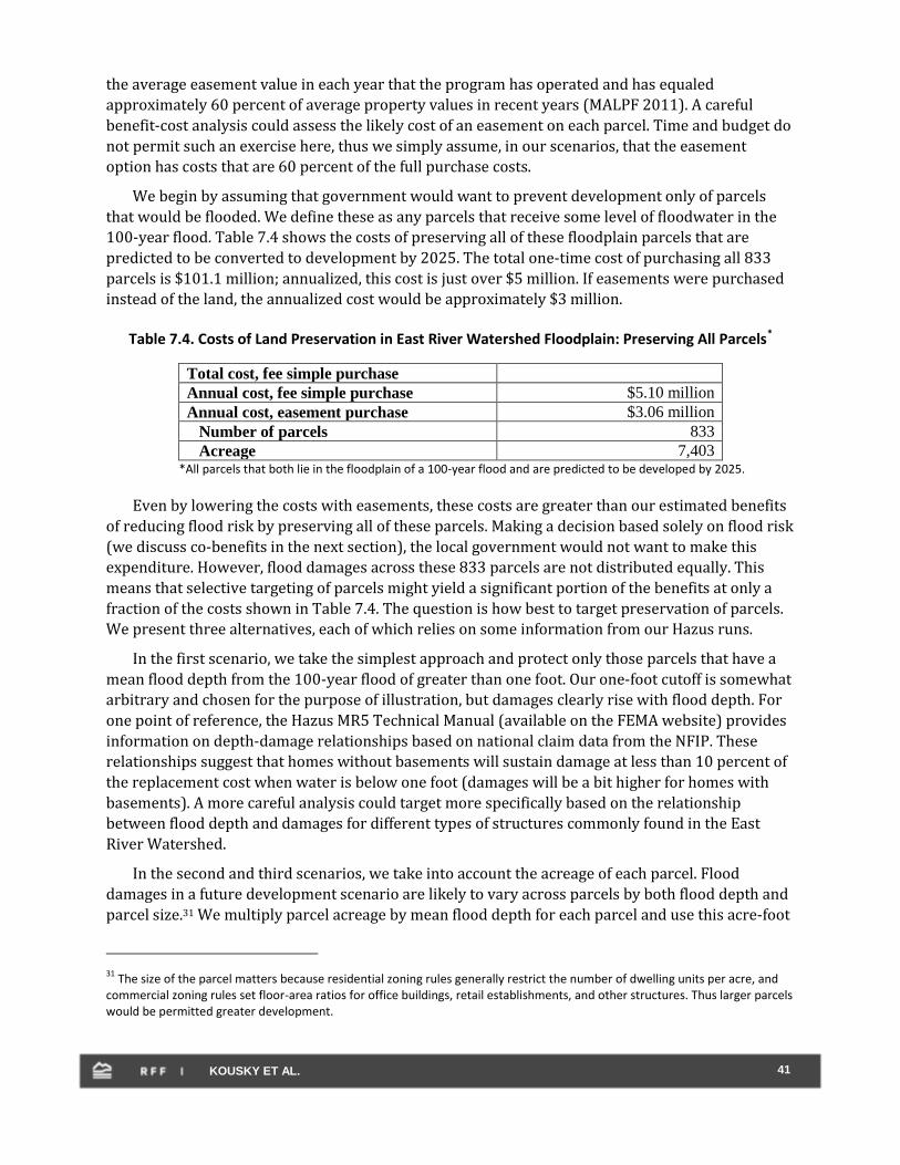
41 KOUSKY ET AL.

the average easement value in each year that the program has operated and has equaled

approximately 60 percent of average property values in recent years (MALPF 2011). A careful

benefit-cost analysis could assess the likely cost of an easement on each parcel. Time and budget do

not permit such an exercise here, thus we simply assume, in our scenarios, that the easement

option has costs that are 60 percent of the full purchase costs.

We begin by assuming that government would want to prevent development only of parcels

that would be flooded. We define these as any parcels that receive some level of floodwater in the

100-year flood. Table 7.4 shows the costs of preserving all of these floodplain parcels that are

predicted to be converted to development by 2025. The total one-time cost of purchasing all 833

parcels is $101.1 million; annualized, this cost is just over $5 million. If easements were purchased

instead of the land, the annualized cost would be approximately $3 million.

Table 7.4. Costs of Land Preservation in East River Watershed Floodplain: Preserving All Parcels*

Total cost, fee simple purchase $101.1 million

Annual cost, fee simple purchase $5.10 million

Annual cost, easement purchase $3.06 million

Number of parcels 833

Acreage 7,403 *All parcels that both lie in the floodplain of a 100-year flood and are predicted to be developed by 2025.

Even by lowering the costs with easements, these costs are greater than our estimated benefits

of reducing flood risk by preserving all of these parcels. Making a decision based solely on flood risk

(we discuss co-benefits in the next section), the local government would not want to make this

expenditure. However, flood damages across these 833 parcels are not distributed equally. This

means that selective targeting of parcels might yield a significant portion of the benefits at only a

fraction of the costs shown in Table 7.4. The question is how best to target preservation of parcels.

We present three alternatives, each of which relies on some information from our Hazus runs.

In the first scenario, we take the simplest approach and protect only those parcels that have a

mean flood depth from the 100-year flood of greater than one foot. Our one-foot cutoff is somewhat

arbitrary and chosen for the purpose of illustration, but damages clearly rise with flood depth. For

one point of reference, the Hazus MR5 Technical Manual (available on the FEMA website) provides

information on depth-damage relationships based on national claim data from the NFIP. These

relationships suggest that homes without basements will sustain damage at less than 10 percent of

the replacement cost when water is below one foot (damages will be a bit higher for homes with

basements). A more careful analysis could target more specifically based on the relationship

between flood depth and damages for different types of structures commonly found in the East

River Watershed.

In the second and third scenarios, we take into account the acreage of each parcel. Flood

damages in a future development scenario are likely to vary across parcels by both flood depth and

parcel size.31 We multiply parcel acreage by mean flood depth for each parcel and use this acre-foot

31

The size of the parcel matters because residential zoning rules generally restrict the number of dwelling units per acre, and commercial zoning rules set floor-area ratios for office buildings, retail establishments, and other structures. Thus larger parcels would be permitted greater development.

42 KOUSKY ET AL.

measure as a proxy for the expected magnitude of flood damages to rank the parcels. In Scenario 2,

we assess the costs of preserving those parcels that account for 90 percent of the total damages

using this acre-foot measure. The 90 percent figure is chosen arbitrarily. In a more complete

analysis, one could try alternatives to more carefully maximize the difference between benefits and

costs.

Finally, in Scenario 3, we divide this acre-foot measure of damages into the costs, as measured

by property values, to obtain an estimate of the cost-effectiveness of protecting each parcel from

development. By cost-effectiveness, we mean the cost per acre-foot of flooding avoided for each

parcel. These cost-effectiveness numbers vary greatly across parcels both because property values

(and thus costs) vary greatly and because the acre-foot measure of flooding (benefits) varies

greatly, though the variance in property values is more substantial. We also find a small negative

correlation between the property values and the acre-feet of flooding, which further contributes to

the wide range in values. The cost-effectiveness estimates range from a low of $26 per acre-foot to a

high of $171 million per acre-foot. The median is $9,959 per acre-foot. The third scenario preserves

only those parcels that are below this median—that is, we target the most cost-effective parcels,

those with the lowest cost per acre-foot of flooding. Again, choosing the median is somewhat

arbitrary, but it provides a benchmark for further analysis and serves to illustrate how costs can

vary depending on how parcels are targeted.

The results for these three targeting scenarios are shown in Table 7.5. As expected, all three

have lower costs than the baseline case above, since fewer parcels are purchased and preserved

from development. In Scenario 1, where we purchase only those parcels that receive more than one

foot of water in the 100-year flood, the annual cost of a fee simple purchase is $3.7 million. In this

case, 69 percent of all flooded parcels slated for development are purchased—575 of the 833

parcels. This accounts for 63 percent of all acreage, 4,646 acres compared with 7,403 acres. In

Scenario 2, which targets based on both flood depth and acreage, far fewer parcels are purchased—

328 of the 833 total. However, a greater amount of acreage ends up protected—6,385 acres, or 86

percent of all acreage that lies in the floodplain and would be developed by 2025. Because far fewer

parcels are being purchased, the cost of Scenario 2, at $1.15 million for a fee simple purchase, is

much less than Scenario 1.

43 KOUSKY ET AL.

Table 7.5. Costs of Land Preservation in East River Watershed Floodplain: Three Alternative Targeting Scenarios*

Scenario 1: targeting based on flood depth

Total cost, fee simple purchase $72.9 million

Annual cost, fee simple purchase $3.67 million

Annual cost, easement purchase $2.20 million

Number of parcels 575

Acreage 4,646

Scenario 2: targeting based on flood depth

and parcel acreage

Total cost, fee simple purchase $22.8 million

Annual cost, fee simple purchase $1.15 million

Annual cost, easement purchase $690,000

Number of parcels 328

Acreage 6,385

Scenario 3: targeting based on costs, flood

depth, and parcel acreage

Total cost, fee simple purchase $9.8 million

Annual cost, fee simple purchase $496,000

Annual cost, easement purchase $298,000

Number of parcels 417

Acreage 6,379 *All parcels that both lie in the floodplain of a 100-year flood and are predicted to be developed by 2025.

Finally, Scenario 3 has the lowest costs of all, less than $500,000 in annual terms for a fee

simple purchase and even less for purchase of easements. This estimate is less than half the cost of

Scenario 2, even though 89 more parcels are purchased. But of the 328 parcels preserved in

Scenario 2, about 83 percent are also preserved in Scenario 3. The acreage of land preserved from

development is virtually the same as in Scenario 2. Scenario 3 is thus acquiring more small, cheap

properties. This option shows how costs of a land conservation program can be minimized if the

cheaper parcels are targeted for conservation. This approach doesn’t just look at costs, of course; by

assessing the costs per acre-foot of damages avoided, it is essentially taking a “bang for the buck”

approach and trying to get as much flood protection as it can with its land conservation dollars.

The differences in parcels preserved among the base case and the three scenarios can be seen in

Figure 7.1. The base case preserves many more parcels—they trace the 100-year floodplain of the

East River and its tributaries. The three scenarios all target parcels for less overall acreage

preserved. The parcels preserved seem very similar in Scenarios 2 and 3, since 83 percent of those

preserved in Scenario 2 are also in Scenario 3, and the parcels are small. All the targeting scenarios

avoid preserving some parcels in the downtown core, where development value may outweigh

flood risk. Figure 7.1 also shows agricultural and natural areas projected for the future to see the

proximity of preserved parcels to other areas of open space or development.

44 KOUSKY ET AL.

Figure 7.1. Parcels Preserved in Base Case and Scenarios 1–3

To accurately compare costs, local governments should obtain new benefit estimates for each

scenario. Here, we presented benefit numbers only for preserving all the land slated for future

development. Clearly, all the benefits will be obtained by only focusing on those properties that are

Base Case Scenario 1

Scenario 2 Scenario 3

45 KOUSKY ET AL.

in the floodplain, as we do in the base case—that is, while the future scenario had more

development outside the floodplain, these properties will not sustain flood damage and thus

preventing them from developing will not generate flood damage reduction benefits. What fraction

of the benefits will be achieved with our targeted scenarios is unclear. It seems safe to assume that

multiplying depth by acreage, as we do here, will at least roughly proxy for flood damages and that

a large fraction of benefits would be achieved with our targeted cases. Costs are much lower than

the benefits estimated above for our third case, and this scenario would very likely pass a cost-

benefit test. Our simple analysis, even given all the caveats we have mentioned, suggests that some

targeted preservation of open space in the watershed would produce economic net benefits to

Brown County.

Local decisionmakers can use the last approach on its own, thereby saving time and money

running the Hazus model to obtain property damage estimates from flooding in alternative land-

use scenarios. In other words, a cost-effectiveness analysis can substitute for a full benefit-cost

analysis. It is also useful when the budget for land or easement purchases is fixed. The county (or

conservation agency or land trust) can pick off the most cost-effective parcels for flood protection

purposes until the budget is exhausted. We emphasize that such an analysis is not a perfect

substitute for fully assessing the benefits and costs, including the important co-benefits of land

conservation that we discuss in Section 8, but it is a useful first step.

7.3. Improving Efficiency and Cost-effectiveness: Better Targeting of Parcels

The problem of targeting parcels for the purpose of reducing flood damages resembles policy

problems in other realms, such as the design of conservation areas to preserve biodiversity, or

riparian restoration programs to improve drinking water quality downstream in a watershed. In

the natural and physical sciences, one standard approach uses either a single biophysical criterion

or a set of such criteria (often combined into a single index) to rank individual parcels or sites in

terms of the benefits delivered by a policy intervention (see, e.g., Dobson et al. 1997; Qiu 2010). For

example, Yeo and Guldmann (2006) develop model land-use policies to reduce nonpoint source

pollution from stormwater runoff in the Old Woman Creek watershed in the southwestern basin of

Lake Erie. They relate peak discharge to land-use variables and then simulate optimal future land

use in the watershed, so as to minimize peak discharge at the creek’s outlet. Where policy analysis

is performed in these cases, the policy prescription is first to fund the intervention that offers the

greatest biophysical benefit, and then to continue down the list until the budget is exhausted. A

related method from the planning literature is a “land-use suitability” analysis, which is designed to

rank the suitability of sites for future land uses based on a set of weighted requirements,

preferences, or other factors (Malczewski 2004).

Our first two targeting scenarios above, taken without any calculation of costs, could be used in

a similar way as in these studies. For example, one could purchase parcels with the greatest mean

flood depth first and continue purchasing until the budget is exhausted, or one could purchase

parcels with the greatest damage in terms of flood depth and acreage.

An economically efficient approach to targeting parcels to reduce flood damages would

consider (1) the monetized benefits of intervention at each potential site (rather than just

biophysical benefits), taking into account any spatial correlation across sites; and (2) the costs of

each potential site in the site selection phase (Ando et al. 1998). An efficient ranking would then

select parcels according to their benefit-to-cost ratio, until the budget is exhausted (Ferraro 2003).

46 KOUSKY ET AL.

Although we stop short of monetizing the full benefits of floodplain land preservation (see

Section 8), our third scenario above does take costs into account in the ranking and selection of

parcels and is thus preferable from an economic perspective. This distinction is particularly

important (1) when the benefits and costs of parcel selection are positively correlated (high-benefit

parcels are also expensive to preserve); (2) when costs are more variable than benefits across

space; and (3) when the budget allows only a small fraction of the desired amount of preservation.

In each of these cases, selecting parcels according to the amount of benefit generated per dollar

spent will result in greater net benefits than selection on the basis of benefits alone (Ferraro 2003;

Newburn et al. 2004; Messer 2006; Newbold and Siikamäki 2009). In our case, the first and third

points are valid. Costs are more variable than benefits over space, and a typical local government

budget would likely allow only a small fraction of desired preservation. If benefits and costs were

also positively correlated (they are negatively correlated in our case), the differences in parcels

selected under Scenario 3 and those in Scenarios 1 and 2 might be even greater (with resulting

consequences for net benefits). Local governments should consider these rules of thumb in

designing local land-use policies to reduce flood damages.

The constrained optimization methods used to determine the economically efficient set of

targeted land parcels to achieve a certain policy goal within a specified budget combine economics,

the natural and physical sciences, and operations research (Siikamäki and Newbold 2009). We have

done something much less precise here. Nonetheless, some of the most important intuition arising

from these more careful methods is illuminated by our simple scenarios.

8. Co-Benefits and Co-Damages Associated with Flood Damage Mitigation Policies

If land-use policies to reduce flood damages also create or preserve additional open space, or if

they change the distribution of open space across the local landscape, recreational opportunities

may be an important co-benefit of such policies. In addition, if these policies reduce or redistribute

impervious cover, affecting stormwater and other types of runoff, they may also improve water

quality within and downstream of the East River watershed, providing additional co-benefits. A

significant local water quality modeling effort, beyond the scope of this study, would be required to

quantify the effects of land-use changes like those we simulate in Hazus on local and regional water

quality. Nonetheless, we can draw on existing literature to describe both the potential

consequences and the range of estimated economic values of these types of water quality changes.

We also can draw from the large economics literature on the value of open space to provide some

information on the benefits of increased green infrastructure in the watershed. A full benefit-cost

analysis of specific land-use policies to reduce flood damages would incorporate all of these

monetized benefits.

8.1. Effects on Water Quality

Essentially all of the LFRB’s water bodies, including the East River and its tributaries, are

impaired (Cadmus 2010). Future increases in extreme precipitation will exacerbate runoff and

further degrade water quality. Section 2.5 described the contribution of agricultural land in the

ERW to water quality problems, particularly eutrophication and other problems stemming from

excessive flows of nutrients to area waterways. Increased runoff from agricultural fields and

combined animal feeding operations due to increases in extreme precipitation could put surface

47 KOUSKY ET AL.

water quality and potentially groundwater quality at risk (Wisconsin DNR 2006; Lowery et al.

2009).

However, the development and urbanization that are the focus of the future flood-damage

assessment Section 4 also pose risks to water quality. As of 2003, more than 225 research studies

had documented the adverse consequences of urbanization for hydrologic, physical, water quality,

and biological indicators in small urban streams and receiving waters (Center for Watershed

Protection 2003). Construction activities during the transition from agricultural land or open space

to residential and commercial development are significant sources of sediment, even when erosion

control practices are followed (Nelson and Booth 2002). Once land is developed, the percentage of

impervious cover grows, intensifying the problem of urban runoff, as described in Figure 8.1. The

percentage of land covered by impervious surface associated with various types of development

varies widely. A survey done by the village of Howard, outside the ERW but within the LFRB,

suggests that impervious surface covers 7 to 34 percent of single-family residential lots (with the

percentage increasing monotonically as lot size shrinks) and 42 to 75 percent of commercial and

industrial parcels (Fink 2005).32 The impervious cover on agricultural land in the ERW is not

described in the literature, but for comparison, impervious surface on agricultural land abutting

suburban development in the Chesapeake Bay region covers less than 2 percent of land area

(Cappiella and Brown 2001).

In the ERW’s Baird Creek subwatershed, a significant contributor to water quality problems in

the East River and Green Bay, urban land covered 18.5 percent of the land area in 2004 but

contributed 60 to 70 percent of the total sediment load during summer precipitation events (Fink

2005). In addition, storm event concentrations of total phosphorus in Baird Creek are significantly

higher on the more rapidly urbanizing South Branch than on the North Branch, with its higher

concentration of agricultural land use (Fink 2005).

However, the potential effect of urbanization in the watershed on water quality is ambiguous.

Though the fraction of impervious cover is greater in urban areas, the concentrations of nutrients in

agricultural runoff may be higher than from urban runoff. A careful water quality study of the LFRB

suggests that if the urban area in the basin doubled by 2030, with no change in the management of

urban runoff, total suspended solid loads from the LFRB to Green Bay would increase, relative to

the 2000 baseline, by 2.3 percent, but total phosphorus loads would decrease by 16.5 percent

(Baumgart 2005).33 If areas urbanized after 2000 adopted more stringent stormwater mitigation

practices than older urban areas, both sediment and phosphorus loads to Green Bay from the LFRB

could be significantly reduced (Baumgart 2005).

On the other hand, if land-use policies to reduce flood damages cause a significant amount of

land currently developed (or likely to be developed in the future) for urban or agricultural purposes

to be converted to open space, water quality will improve. In the extreme, if the entire LFRB (with

32

During the establishment of its stormwater utility, the village used aerial photography to estimate these percentages, using a random sample of 30 properties from each of 13 residential and commercial land-use subcategories.

33 This modeling effort uses the Soil and Water Assessment Tool (SWAT) to predict the effect of several land-use-change

scenarios on pollutant loads to Green Bay from the LFRB. The authors emphasize that the simulated changes in TSS and P loads depend on the assumed yields of these pollutants from urban versus agricultural sources (since most of the land expected to urbanize between 2000 and 2030 will convert from agriculture). The information used to calibrate the modeling of agricultural runoff was developed specifically for the LFRB; the urban component used data primarily from Wisconsin but not specific to the LFRB (Baumgart 2005).

48 KOUSKY ET AL.

the exception of wetlands) reverted to forested land, TSS loadings from the subbasin to Green Bay

would be reduced by an estimated 93 percent, and total phosphorus loadings would fall by almost

90 percent (Baumgart 2005). We mention this not as a realistic or desirable scenario but simply to

illustrate the strong relationship between land use and water quality in the region.

A flood damage mitigation policy that alters the spatial distribution of open space and

residential, commercial, and agricultural development will affect water quality. A full benefit-cost

analysis of any such policy would monetize water quality improvements as co-benefits, or include

water quality degradation on the cost side, or both.

Figure 8.1. Effect of Urbanization on Stormwater Discharges

Source: U.S. Environmental Protection Agency. 2010. Stormwater rulemaking consultation with state and local governments. Available at http://www.naco.org/legislation/policies/Documents/Energy, Environment,Land%20Use/EPA%20SW%20Rulemaking%20Briefing.pdf.

8.2. Monetizing Water Quality Co-Benefits or Co-Damages

Environmental and natural resource economists have developed methods to estimate the

benefits of preserving environmental goods and services and, conversely, the damages when such

resources are destroyed or depleted. The economic benefit provided by an environmental good or

service is the sum of what all members of society would be willing to pay for it (or the minimum

compensation they would be willing to accept to preserve their well-being after the damage is

done). For resources traded in markets, such as oil, land, timber, and crops, the value of small

changes in quality and quantity can be measured by observed prices; this is why, in estimating the

direct economic losses from flooding in Section 4, we used the value of structures and furnishings

49 KOUSKY ET AL.

on developed land, and crop losses on agricultural land.34 In competitive markets, prices reflect

both the marginal cost of producing the good to suppliers and the marginal value to consumers.

Prices are readily observed and constantly updated.

For goods and services that are not traded in markets (“nonmarket goods”), such as water

quality and recreational opportunities, the methods are less straightforward, though the basic idea

is the same. Economic techniques—theoretically consistent with market prices and demand and

supply functions—must be used to estimate economic value.35 Two broad classes of methods are

used for this purpose: behavioral (revealed preference) and attitudinal (stated preference). Both

types of methods are designed to measure the value of goods and services in the absence of explicit

markets. Revealed-preference methods measure values by observing choices that people make in

markets, though not direct markets for the “good” being valued. For example, when people travel to

a recreation site, they value their visit to the site at least as much as they paid to travel there.

Stated-preference methods generally use surveys to assess the trade-offs people would be willing

to make for nonmarket goods by creating hypothetical scenarios that simulate market transactions.

In the case of water quality improvements that might be achieved through land-use policies

designed to mitigate flooding from extreme precipitation, several categories of market and

nonmarket benefits are possible. Fish catch rates might improve in the ERW, the LFRB more

generally, and even downstream in Green Bay, affecting both commercial and recreational fishing.

Beach water quality might improve for swimmers in Green Bay, reducing the frequency of beach

closures or otherwise improving local swimming experiences, whether aesthetically (e.g., water

clarity, odor) or in terms of reduced health risk. Wildlife viewing (e.g., bird watching) and hunting

opportunities could improve. Homeowners’ property values could also increase as a function of any

of these listed impacts or other factors.

If a water quality modeling effort produced estimates of the water quality consequences of the

land-use changes simulated in Section 4, a formal “benefit transfer” analysis or a new original

valuation study could be conducted to carefully translate biophysical water quality improvements

into dollar values. Though we know of no estimates of the economic value of specific water quality

improvements in the ERW, let alone those related to a reduction in the runoff intensity of

precipitation events, we can summarize a range of potentially relevant estimates by drawing on a

substantial economic literature on nonmarket benefit estimation. The reader should be cautious in

interpreting these estimates; they merely illustrate the point that water quality improvements can

have substantial economic value.

About three-quarters of published estimates of the economic value of nonmarket goods and

services in the United States that are provided by water quality are recreational benefit studies, and

recreation may constitute the greatest share of economic benefits from water quality

improvements (Van Houtven et al. 2007). Perhaps the estimates most relevant to our purposes are

34

For larger changes in market goods, prices would also be used as a measure of economic value, but current prices could not necessarily play this role, as they would likely shift with market-level changes in demand and supply. For example, if a flood wiped out dairy production in Wisconsin for several months, and this significantly reduced supply, the market price of milk might rise. An assessment of agricultural losses from the flood would have to take this into account.

35 More detailed recent summaries of these techniques and many applications, prepared for the noneconomist, can be found in

Mendelsohn and Olmstead (2009), and Bockstael et al. (2000).

50 KOUSKY ET AL.

those summarized in a recent study of the economic value of water quality improvements in the

Great Lakes (Austin et al. 2007b).

Recreational fishing represents a substantial portion of the benefits of water quality

improvement in that study. Table 8.1 summarizes estimates of the economic benefit of increasing

fish catch rates in the Great Lakes by 10 percent, in dollars per angler per day. They range from

$0.26 per day for Michigan anglers for trout and salmon in Lake Michigan, to $3.17 for Wisconsin

anglers for all species in Green Bay. The higher value by Green Bay anglers for a 10 percent increase

in catch rates for all species is roughly consistent with adding up the value estimates (to Green Bay

anglers) for major individual species in Table 8.1.36

Table 8.1. Estimated Value to Great Lakes Anglers of 10 Percent Increase in Fish Catch Rates

Study Fish species Lake Affected anglers

Benefit per

angler per day

Breffle et al. 1999 All species Michigan (Green

Bay)

Wisconsin anglers near

Green Bay, 1998

$3.17

Jones and Lupi 2000 Trout, salmon Michigan Michigan anglers,

1983-84

$0.26

Samples and Bishop

1985

Trout, salmon Michigan Wisconsin anglers near

Lake Michigan, 1979

$0.83

Breffle et al. 1999 Trout, salmon Michigan (Green

Bay)

Wisconsin anglers near

Green Bay, 1998

$0.95

Breffle et al. 1999 Walleye Michigan (Green

Bay)

Wisconsin anglers near

Green Bay, 1998

$0.49

Breffle et al. 1999 Smallmouth

bass

Michigan (Green

Bay)

Wisconsin anglers near

Green Bay, 1998

$0.80

Breffle et al. 1999 Yellow perch Michigan (Green

Bay)

Wisconsin anglers near

Green Bay, 1998

$0.92

Source: Austin et al. (2007b), Table B-2.

A critical step in monetizing the water quality benefits associated with any land-use change

policy is establishing a link between that policy and its anticipated biophysical impact. If a land-use

policy is implemented to reduce flood damages in the ERW, by how much will this policy improve

water quality (for each affected contaminant) and therefore fish catch rates downstream in Green

Bay? The Great Lakes study by Austin et al. (2007b) offers a list of goals for Great Lakes restoration

that are broadly relevant to this issue. For example, the fish catch rate changes they value result

from several significant proposed pollution management efforts in the Great Lakes region as a

whole: a 40 to 70 percent decrease in livestock’s contribution to nonpoint source pollution loading,

restoration of 550,000 acres of wetlands over five years, restoration of 35,000 acres of urban and

suburban buffer areas, and a 40 percent reduction in soil loss in 10 regional watersheds, to name a

few. If these measures and others were taken, the study anticipates a 30 to 75 percent increase in

fish abundance in the lakes, valued at $1.1 billion to $5.8 billion. A similar analysis would need to be

36

Values would also be expected to increase for a greater improvement in fish catch rates; for example, the same study that estimated a value of $3.17 per angler per day for a 10 percent increase in Wisconsin anglers’ catch rates of all species in Green Bay also estimated a value of $15.82 per angler per day for a doubling of the all-species catch rate (Breffle et al. 1999).

51 KOUSKY ET AL.

completed for the ERW specifically, to translate expected water quality impacts from new land-use

policies, to impacts on fish abundance, to the economic value of increases in fish catch rates.37

Similarly, improvements in beach water quality for recreational swimmers would have

economic value. The Great Lakes study anticipates a 20 percent reduction in beach closings and

advisories as a result of federal and state investment in the Great Lakes Restoration Program, as

well as a 5 percent improvement in beach water clarity; the combined value of these improvements

to swimmers would be $4.5 billion to $5.5 billion. Obviously, improvements in the ERW, or even the

LFRB, alone, would be on a much smaller scale. But even studies of changes at individual beaches

suggest a significant value of improved water quality. For example, for beachgoers at Ohio’s

Maumee Bay State Park on Lake Erie, the aggregate annual benefit of reducing bacterial

contamination from runoff (which causes beach closures) using constructed wetlands is estimated

to be $6.19 million (Awondo et al. 2011).

Higher fish catch rates, better swimming opportunities, and other benefits of water quality

improvement accrue not just to periodic visitors to Green Bay and the surrounding watersheds, but

also to property owners in the region. Economic analyses have linked improvements in water

quality with increases in local property values, in many cases using “hedonic property models,”

which statistically estimate the relationship between changes in local water quality and observed

changes in home prices.38 For example, residential waterfront land prices in the Chesapeake Bay

region increase with reductions in fecal coliform contamination (Leggett and Bockstael 2000), and

lakefront home values in Maine are lower on lakes where water clarity (measured by Secchi depth)

is poorer (Poor et al. 2001; Boyle et al. 1999).

Perhaps the most relevant research on this issue, given the focus of this study, is a recent study

of property owners’ total willingness to pay for improvements in Green Bay water quality through

reductions in nonpoint source pollution (Moore et al. 2011). The authors use a stated-preference

survey rather than a hedonic analysis. Their survey asked homeowners to value a summer average

water clarity improvement of four feet (Secchi depth) in lower Green Bay; the survey also explained

the links between runoff and water clarity, and between water clarity, wildlife abundance, and

recreation (Moore et al. 2011). The survey asked each respondent for a “yes or no” vote on a

hypothetical referendum to reduce nutrient runoff to Green Bay, at the cost of an increase in state

and local taxes ranging from $50 to $1,000 per year (these prices were randomly assigned, and

each homeowner faced a single price). The estimated average annual willingness to pay varies

significantly with homeowners’ distance from the bay, current water quality in their area of the bay,

frequency of recreation on and near the bay, income, and many other factors. The main model in the

study suggests that local property owners’ aggregate willingness to pay for a nutrient reduction

program resulting in an average four-foot improvement in summer water clarity in the bay is more

than $10 million per year (Moore et al. 2011).

37

Anglers in Green Bay, Lake Winnebago, and the Lower Fox River are also willing to pay to avoid fish consumption advisories due to PCB contamination (MacNair and Desvousges 2007). If land-use policies to reduce flood damages affected the distribution and transport of PCB-laden sediments in the LFRB and Green Bay, a full benefit-cost analysis of these policies would incorporate the value of these effects as well.

38 To be more precise, hedonic models express the price of a product as a function of the characteristics or attributes of the

product; when the model is econometrically estimated using data on market prices and attributes, the resulting estimated coefficients represent the marginal implicit prices of the attributes.

52 KOUSKY ET AL.

8.3. Recreational and Other Co-Benefits Directly from Land-Use Change

In addition to reducing flooding and improving water quality, natural areas and open space can

provide a range of other direct benefits, such as enhanced recreational opportunities, improved

wildlife habitat, reductions in urban heat island effects, air quality benefits, and general aesthetic

benefits to nearby residents. The magnitudes of the benefits depend on several factors, including

the type of open space (forested, wetland, agricultural, developed recreational space, or other), the

ownership structure (public versus private), and proximity to centers of population and other

protected land uses.

The recreational benefits of green infrastructure have been emphasized by many park

proponents and advocates for land conservation (e.g., Nashville: Naturally 2011), but these benefits

depend critically on public access. Thus undeveloped land that remains in private ownership may

provide flooding and water quality benefits but little or no opportunity for recreation if public

access is restricted. Placing a conservation easement or deed restriction on the land may not

entirely address this accessibility issue. In addition, recreational benefits depend on the attributes

of the property. For example, benefits from camping and hiking depend on the presence of

campsites and trails; benefits from bird watching and wildlife viewing may be high for forested

lands or wetlands but relatively low for developed parks; benefits from sports-related recreation

depends on the existence of ball fields and other developed landscapes.

Improved wildlife habitat may contribute to recreational benefits—it enhances wildlife viewing

and bird watching—but may also provide a “nonuse” value to residents who value knowing that

habitat has been retained or restored even if they do not plan to spend time viewing wildlife

themselves (Freeman 2003). Other nonuse benefits may include the simple aesthetic benefits of

more green space and/or benefits from reduced congestion associated with development. These

benefits may be difficult to quantify separately but can be a part of the overall benefits of green

infrastructure. Finally, urban heat island benefits from tree canopy and other green infrastructure

have been documented for many cities, but it is unlikely that these benefits would be large in a city

the size of Green Bay located in a northern area with mild summers. Similarly, trees and other

plants can reduce urban smog, or ground-level ozone, but Green Bay is not on EPA’s list of ozone

nonattainment areas; thus these benefits should also be small in our study area.

8.4. Monetizing Recreation and Other Co-Benefits from Open Space

McConnell and Walls (2005) comprehensively review the economics literature on the value of

open space, summarizing more than 60 studies that assess values of urban and suburban parks,

natural areas, greenbelts, forest reserves, wetlands, and farmland. The studies rely on the

techniques introduced in Section 8.2: a revealed-preference, hedonic property value approach and a

stated-preference, survey-based approach.

Hedonic property models have proved particularly useful for estimating the value of both

nonmarket environmental amenities, such as parks and open space, and disamenities, such as air

pollution, noise, and proximity to noxious facilities like landfills. The methodology has the

advantage of relying on “revealed” data about preferences in the marketplace, but it has the

potential disadvantage of missing some of the benefits of the amenity. This may be the case if

benefits accrue to residents outside the housing market used in the analysis. It also may be the case

if nonuse values are large and not fully capitalized into property values. In addition, while the

53 KOUSKY ET AL.

hedonic technique is good at measuring marginal changes in open space—studies have used

distance to open space, open space acreage, percentage of land surrounding a house that is in open

space, and combinations of these metrics as explanatory variables—it is less well suited to valuing

large nonmarginal open space projects.

Stated-preference surveys have been used extensively to value open space. These methods have

the advantage of capturing the full range of benefits and of relying on carefully constructed

experiments such that the nature of the good being valued is clear. They also can adequately

address nonmarginal changes in amenities. But they have the disadvantage, long recognized in the

economics literature, of relying on hypothetical constructs. Well-designed and executed studies

minimize this problem, but it is difficult to eliminate it entirely.

Some recent studies have developed a new technique for valuing open space and other spatially

differentiated environmental amenities using general equilibrium models of urban land and

housing markets (Klaiber and Phaneuf 2010; Walsh 2007). These models, often referred to as

equilibrium sorting models (Epple and Sieg 1999; Bayer and Timmins 2007), assume that

households choose their locations in response to both their own preferences and the existence of

spatially differentiated amenities and public goods. The studies use data on both household

characteristics and housing and neighborhood characteristics (as in hedonic models) to obtain the

values of these public goods. The estimation procedure accounts for the fact that households may

sort into neighborhoods with certain characteristics, causing willingness to pay to be a driver of

open space amenities; the opposite relationship (which hedonic models attempt to estimate) is also

true. Policy simulations in these models account for the new equilibrium brought about by the

policy. For example, provision of parkland or open space would shift households around on the

landscape and alter housing prices; these changes affect the welfare estimates for the policy. The

results from these studies often show significant differences between the partial equilibrium and

general equilibrium estimates, justifying the use of this new approach. Like the basic hedonic

property value studies, however, this methodology assumes that open space values are fully

capitalized into property values.

Recreation benefits are sometimes measured using the travel cost methodology, which uses

observations of individuals’ out-of-pocket travel expenditures and time costs to get to a recreation

site to infer values. Since the technique was developed, thousands of travel cost studies have been

published. However, they tend to focus primarily on state or national parks located far from

population centers and not on urban open space. Moreover, they are usually focused sharply on

specific recreational activities and are not related to changes in land use. Thus, these approaches

are less relevant to our study.

The open space studies reviewed by McConnell and Walls (2005) suggest a wide range in the

value of recreational benefits to local residents. Values within individual studies vary by location,

type of open space, and household type—in fact, this result is emphasized as a finding by many

authors (Anderson and West 2006; Irwin 2002; Klaiber and Phaneuf 2010)—and values across

studies vary even more widely. In fact, comparison across studies is complex given the different

methodologies and open space metrics used. This makes benefits transfer to a new area, such as the

ERW, difficult. In a study of parks in the Twin Cities, Anderson and West (2006) find that city

residents would be willing to pay an additional $600 to live 200 meters closer to a regional park or

natural area, but suburban residents were found to have no positive value from being closer to such

parks. Irwin (2002), in a study of Maryland counties, estimated that conversion of one acre of

54 KOUSKY ET AL.

developable farmland to permanently protected conservation land (such as farmland under a

permanent easement) would be worth an average of $3,300 per household, or 1.87 percent of the

price of an average house, but converting one acre to public land (such as a park) was worth only

$994. Thorsnes (2002) in a study of forest reserves within subdivisions in Michigan found that this

kind of open space had no impact on house prices unless the houses were adjacent to the reserve, in

which case the reserve added 2.9 to 6.8 percent to average house prices.

Studies of wetlands show a range of values depending on the type of wetland and location.

Reynolds and Regalado (1998) find that forested and emergent palustrine wetlands, which account

for 94 percent of the wetlands in their rural Florida study, have negative effects on property values.

Scrub-shrub and shallow pond wetlands, however, appear to have a positive effect. Doss and Taff

(1996) use data from Ramsey County, Minnesota (suburban St. Paul), to estimate how distance to

four types of wetlands affects property values. They find that as the distance to forested wetlands

decreases, property values decrease, but as distance to the other types of wetlands—open water,

emergent vegetation, and scrub-shrub wetlands—decreases, property values rise. Mahan et al.

(2000), on the other hand, in a study of the Portland, Oregon, housing market, find that wetland

type does not matter and that the price of a house tends to be higher the closer it is to any type of

wetland and the larger that wetland is. Results from two recent open space valuation studies are

shown in Table 8.2. These studies are based on the new equilibrium sorting model approach

described above.

Table 8.2. Value of Open Space from Recent General Equilibrium Spatial Models of Urban Housing Markets

Study area Open space policy simulation Average benefit per household

Wake County, North

Carolina1

5.2% increase in protected open

space (4,176 acres)

$25

Twin Cities metropolitan

area, Minnesota2

2.5% increase in protected

(nonpark) open space (1,128

acres)

$255–$510

1 Walsh (2007).

2 Klaiber and Phaneuf (2010). The benefits vary by proximity to the city center, with the lowest values for households

residing within 10 miles of either Minneapolis or St. Paul, a midrange value for households who live between 10 and 18

miles, and the highest value for households beyond 18 miles.

As with the earlier literature, these newer studies also show wide-ranging estimates of open

space values. Although the techniques, types of open space considered in the policy simulations

(general protected lands but not developed parks), and open space metrics are similar for these

two studies, the average benefit numbers differ by an order of magnitude. In the Klaiber and

Phaneuf (2010) study, the average benefits vary by location. Also, beyond the policy simulation

results shown in the table, Klaiber and Phaneuf find widely varying benefit estimates for different

kinds of open space by household type, a point that the authors emphasize.

Monetization of the potential water quality impacts of the ERW land-use scenarios we simulate

in Section 7.2 is beyond the scope of this study. Nonetheless, land use in agricultural and natural

areas differ in our predevelopment and postdevelopment scenarios by approximately 22,000 acres.

Preventing development on this full acreage would imply a 43 percent increase in open space over

Brown County’s projected future land-use scenario—rather than 48,472 acres in agricultural and

55 KOUSKY ET AL.

natural areas in 2025, the ERW would retain its current level of 70,472 acres. These changes would

undoubtedly create additional economic value, either directly (e.g., from recreational access or

property value increases for nearby developed land) or through improvements in local and regional

water quality. It is possible that the value of these co-benefits would be larger than the benefits of

avoided flood damages, themselves. Consider that, if Brown County’s population increased to about

302,000 in 2025, as in the county’s expected future growth scenario, benefits of $8.71 per

household would create aggregate county co-benefits equal to the value of avoided flood damages

($2.63 million) from our Hazus runs in Section 7.1. This is about one-third of the most conservative

per household benefit of open space from Table 8.2 (which does not include water quality

improvements).

9. Policy Tools for Changing Land Use

The benefit-cost analysis in Section 7 assumes that the government purchases land and retains

it as public open space or that the government purchases the development rights on the properties,

leaving the land itself in private ownership but placing it under easement. Although the easement

approach is less costly than fee simple purchases, both options require a source of funding. In the

last part of this section of the report, we discuss existing funding sources for land conservation in

Wisconsin. But we begin here with a more general discussion of the merits of Purchase of

Development Rights (PDR) programs and a variety of other land-use policy options: Transfer of

Development Rights (TDR) programs, zoning, and development impact fees.

9.1 Purchase of Development Rights

In a PDR program, property owners sell their development rights to either a government

agency or a private conservation organization or land trust; typically, the easements are permanent

and prohibit any development on the land beyond what may be there when the development rights

are sold (usually a single dwelling unit so that the existing residents can remain on the property).

There are advantages and disadvantages to PDRs. First, because they are voluntary, PDRs allow

landowners to make decisions that are in their own best interests. Therefore, unlike zoning

regulations, which set uniform requirements across all parcels in a particular zoning category, PDRs

provide some flexibility, which generally reduces the cost of meeting a particular acreage goal.39 On

the other hand, their voluntary nature means that there is no guarantee any particular parcel will

end up with an easement on it. In addition, although they are less expensive than outright land

purchases, PDRs still impose a heavy financial burden on local governments. This is one of their

most serious drawbacks, particularly in today’s economic environment. Often, local governments

have only a limited budget for land preservation; raising taxes to pay for PDR programs can be

politically unpopular and, because of the cost of public funds, increases the overall social cost of the

program.40 Moreover, when funds are limited and there are more property owners willing to sell

39

Environmental economists have long touted the virtues of incentive-based instruments such as fees, subsidies, and tradable permits for achieving environmental goals for this same reason: unlike command-and-control mandates and regulations, they allow flexibility across individual polluters and thus lead to least-cost outcomes.

40 Because distortionary taxes are used to raise revenues to fund government programs such as PDR programs, the total social

cost of the program includes the welfare loss from those taxes (Browning 1987).

56 KOUSKY ET AL.

development rights than the county can afford to purchase, difficult decisions must be made about

which properties to preserve.

PDRs are a popular land preservation tool used widely across the country. The first PDR

program was instituted in Suffolk County, New York, in 1974, and the American Farmland Trust

estimates that more than 1.3 million acres of farmland has been preserved through such programs

(AFT 2003). The approach is also used beyond agriculture, to protect environmentally sensitive

lands, wetlands, stream buffers, forests, and other lands. Private land trusts have turned

increasingly to purchase (or donation) of easements instead of direct ownership of lands in recent

years. The Land Trust Alliance (2006), an organization that represents local land trusts nationwide,

estimates that 6.2 million acres of land was under easement in 2005, compared with 1.7 million in

direct ownership by land trusts. Over the five years between 2000 and 2005, land under easement

rose 148 percent, swamping the 40 percent growth in land directly owned.

9.2. Transfer of Development Rights

TDRs transfer development from one property to another. Like PDRs, a permanent easement is

attached to the property from which the development rights are sold, but unlike PDRs, those rights

are used to increase development on another property. TDRs are bought and sold in a private

marketplace, with landowners voluntarily selling their rights usually to developers who use the

rights to develop more intensively elsewhere. TDRs require no expenditures of government funds,

and that is one of their most appealing aspects to local governments, especially in the current

economic environment.41

TDR programs work hand-in-hand with the zoning rules established in a community. In the

TDR “receiving” area, for example, the baseline zoning rules allow developers to build a particular

number of houses per acre; with TDRs in hand, developers are given a density “bonus,” a

percentage over the baseline. This is what generates a demand for TDRs. The supply comes from

the TDR “sending” areas, the areas targeted for preservation. If the baseline zoning on those

properties is restrictive, then the profitability of development is low and a greater supply of TDRs

can be expected from landowners.

There are approximately 140 TDR programs in operation in the United States, but very few

have active and functioning TDR markets and a significant amount of acreage preserved from

development (Pruetz 2003; Walls and McConnell 2007). Some research suggests that a limited

demand for additional density in receiving areas, and thus a limited demand for TDRs, is the main

reason for the poor performance of most programs (McConnell and Walls 2009; Kopits et al. 2008;

Walls and McConnell 2007). In many cases, this limited demand is a result of the local government’s

design of the program and accompanying zoning rules.

Some successful programs do exist, however. The Calvert County, Maryland, program has been

quite successful, protecting over 13,000 acres of farmland since the late 1970s through a flexible

and well-functioning market (Walls and McConnell 2007). The Montgomery County, Maryland,

program is often held up as the premier example of a successful program, and indeed, more land

41

Some of the economic efficiency implications of TDRs are described and evaluated in Thorsnes and Simon (1999), Mills (1980), McConnell et al. (2006), and Kopits et al. (2008).

57 KOUSKY ET AL.

has been protected in that program than in any other—some 49,000 acres.42 But the Montgomery

County program relied on very restrictive downzoning of a large area of agricultural land at the

outset of the program: development was reduced from one house per 5 acres to one house per 25

acres (Walls and McConnell 2007). This generated an enormous supply of TDRs. Accompanied by a

robust demand for development in the Washington, D.C., suburbs, the TDR market has been very

active. A handful of other programs around the country have also had some success (Pruetz 2003;

Walls and McConnell 2007).

A recent feature of several TDR programs is the option for developers to pay a fee in lieu to the

local government rather than purchase TDRs from private landowners. This option is given when

developers are unable to close a transaction in the private marketplace. The difficulty of getting

TRD markets going in many locations spurred the move to the fee in lieu option. In these programs,

the local government uses the collected revenues from the fees to purchase land for preservation.43

Many TDR programs target farmland for preservation. Some programs focus on historic

properties; others target land in environmentally sensitive areas to prevent erosion, protect

wetlands, or protect water resources. No programs, to our knowledge, currently target land in a

floodplain, but a TDR program would be ideal for this purpose. Designing and implementing an

effective program are difficult tasks, but the strapped budgets of local governments may lead many

communities to consider the TDR option in the future.

9.3. Development Fees or Taxes

Many economists have suggested a fee or tax per acre as an efficient means to reduce

development and limit sprawl (Brueckner 1997, 2001; Bento et al. 2006). As an incentive-based

instrument, such a fee could be a low-cost way to reduce land in developed uses. In theory, the fee

could vary by location, with developers of the floodplain paying a higher fee per acre than for land

elsewhere. In addition, this approach has the added benefit of raising money for communities,

compared with PDRs and other approaches that rely on expenditures.

Development fees currently exist in many communities. So-called development “impact fees”

are up-front charges applied to new developments to cover the cost of providing public services,

such as roads, sewers, and schools. The basic premise is that new developments should cover the

full marginal costs that they impose on the community; existing residents should not have to pay, in

the form of increased property or other taxes, the additional costs of servicing the new

developments. But the fees are not usually set on a per acre basis; rather, they are one-time fixed

fees charged for each housing unit built, or they vary with the square footage of a house (Walls et al.

2011). Several court cases have determined that impact fees can be set to cover only the marginal

infrastructure costs associated with new development, limiting their use for environmental

purposes and to prevent or reduce development in particular locations. This suggests it may be

difficult to use development fees or taxes to reduce development in the floodplain. Even if such fees

could be used in this way, the land is not permanently protected.

42

Montgomery County is approximately 2.5 times larger than Calvert County. Both counties have protected additional acreage through PDR programs. Total acreage under easement in Calvert County is about 26,000 (McConnell and Walls 2009).

43 Cities with fee in lieu programs include Livermore, California; Scarborough, Maine; Bertoud, Colorado; Clifton Park and

Goshen, New York; and Seattle (Pruetz, personal communication, May 12, 2009).

58 KOUSKY ET AL.

9.4. Zoning

The most direct way that local governments control the amount, location, and density of

development is with zoning. Most counties and municipalities establish commercial, industrial,

residential, and other zoning categories, carefully prescribing the uses that are allowed in each

category and then determining the locations in the jurisdiction for each zoning designation. In

addition, the intensity of use in each category is defined in the zoning code. Residential properties

usually face a specified limit on the number of dwelling units per acre, and there may be several

residential zoning categories in a county. For example, a typical suburban county may have areas

devoted to high-density multifamily uses (perhaps with 12 to 20 dwelling units per acre); areas

permitting medium-density single-family dwellings (3 to 4 dwelling units per acre); and low-

density residential (1 unit per acre). One of the most straightforward ways of limiting total

development in an area is to change zoning to allow fewer dwelling units per acre. In fact, many

communities on the urban fringe have used this approach to try to protect rural lands from

development, often downzoning lands to 1 unit per 10, 20, or even 50 acres.

There are several problems with this approach. First, property owners often view downzoning

as a form of “takings,” since it reduces the value of their land. This may lead to numerous

applications for zoning variances, court battles, and other problems. Second, downzoning can

encourage urban sprawl because houses are built over a larger area of land. And third, zoning is a

blunt policy instrument that is unable to allow for differences in costs of building and preferences

of homeowners and the community that might exist within a zoning designation or particular

geographic area. This is true of zoning density limits and of allowable use zoning, such as

agricultural zoning or conservation zoning. This may prove particularly problematic for floodplains

where flood depths and damages can vary greatly across parcels.

9.5. Summary of Policy Instruments

Table 9.1 summarizes the policy instruments we have discussed here, as well as FEMA buyouts

and a modified FEMA buyout option. The benefits of each instrument depend primarily on how well

it is able to target land parcels that provide the greatest amount of flooding benefits. Some of the

instruments do a better job than others. The costs also depend, to some extent, on targeting but also

on how flexible the instrument is. If a policy allows landowners some choice in their actions, the

lower-cost properties are likely to be preserved first. We also include information on who bears the

costs and on co-benefits of each option. These co-benefits depend, to a great extent, on whether

recreation options are enhanced, and this depends in turn on whether lands are publicly accessible.

Finally, the table includes some other important issues for each policy tool.

9.6. Funding Opportunities for Wisconsin Fee Simple Land Purchase and PDR Programs

States vary widely in their funding of conservation activities (Walls et al. 2009). Some states

have dedicated funding sources from sales tax surcharges, real estate transfer taxes, hunting and

fishing license fees, lottery revenues, bond sales, and various other sources. Other states do not

have such dedicated funds. Even for the ones that do have funds, the sums available vary widely

and are spent in different ways. The primary source of state funding for land conservation in

Wisconsin is the Knowles-Nelson Stewardship Program, which currently provides $60 million per

year for land conservation. The program, which is funded through general obligation bonds, funds

59 KOUSKY ET AL.

land acquisition for the state DNR and provides 50 percent matching grants to local governments

and land trusts for land acquisition, restoration activities, and development of trails and other

amenities. The local matching requirement is typical of state programs that provide conservation

funds to local government. Local government grants will account for only $8 million of the $60

million in FY2011 and 2012.44 Since it began in 1989, the program has protected more than

600,000 acres of land, mostly through its land purchases for DNR. According to the Trust for Public

Land’s Conservation Almanac, Wisconsin ranked 16th among states in conservation spending per

capita over the 1998–2005 period.45

As we mentioned in Section 2, Wisconsin also provides grants to local governments through the

Municipal Flood Control Grant program; this money can be used to acquire land and easements in

the floodplain. Approximately $2.5 million to $3.5 million of funding is available in each two-year

round of funding. Local communities are required to contribute 30 percent matching funds.

Some federal funds for land conservation activities flow to the states through the U.S.

Department of Agriculture’s Natural Resources Conservation Service. NRCS operates the Farm and

Ranchland Protection Program (FRPP), the Wetlands Reserve Program, and the Emergency

Watershed Protection (EWP) Easement Program, among many others. In 2011, Wisconsin had just

under $2 million for purchase of easements on agricultural land through FRPP. This program

requires a 50 percent match by a local government or nonprofit and is focused on prime

agricultural properties that meet specific NRCS criteria. The Wetlands Reserve Program targets

wetlands on agricultural lands. More than $10.6 million was spent in Wisconsin in 2010 protecting

2,589 acres of land. The EWP easement program targets agricultural properties in floodplains that

have had a history of repeated flooding. The federal stimulus sharply increased funding for the

program in 2009. Wisconsin received $19.7 million to purchase easements on 23 properties

comprising 4,000 acres of land (Wisconsin NRCS 2009a). According to American Rivers (2011), a

significant unmet demand for EWP easements exists in Wisconsin: between 2008 and 2010, 66

percent of the acreage that applied to the program was unawarded. EWP program funding has been

cut to zero in the most recent federal budget.

Although sources of funding for land conservation in Wisconsin are not insignificant, they are

probably inadequate, at current levels, to bring about significant protection of lands in the

floodplain. The Knowles-Nelson program and the federal NRCS programs have their own priorities,

so even though flood control may be a co-benefit of some of the land conservation achieved through

those programs, it is not a program focus. The state’s Municipal Flood Control Grant program is

small, and the federal EWP easement program is currently unfunded. In our scenarios analyzed in

Section 4, between 4,600 and 7,400 acres of land in a single watershed in the state was preserved.

As we stated at the beginning of this section, land purchase and PDR programs may not be available

to do the job. Communities need to consider the other policy options to bring about land-use

change.

44

The governor temporarily halted all spending from the program in February 2011. When the state passed its budget, annual appropriations were reduced from $86 million to $60 million. See http://dnr.wi.gov/stewardship/ for more details on the changes to the program.

45 The Conservation Almanac is available at http://www.conservationalmanac.org/secure/index.shtml.

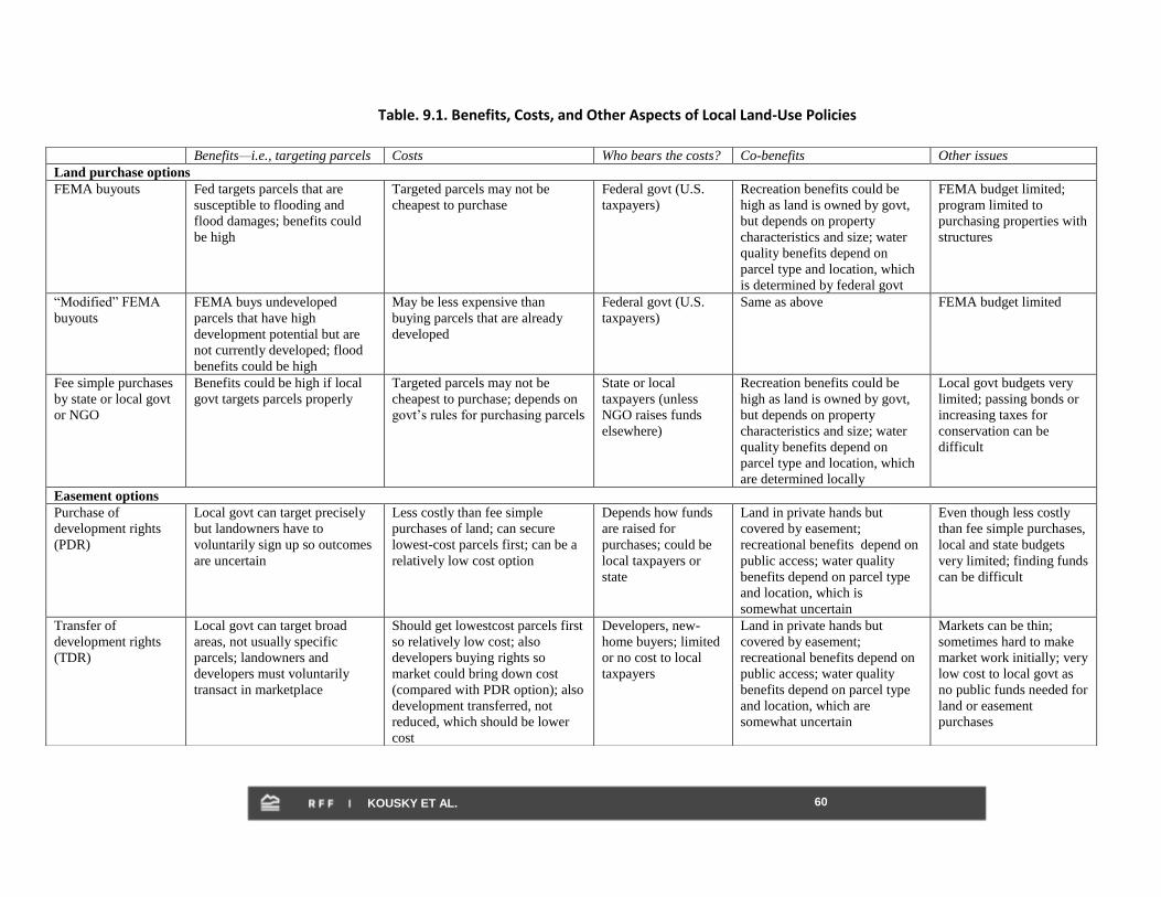
60 KOUSKY ET AL.

Table. 9.1. Benefits, Costs, and Other Aspects of Local Land-Use Policies

Benefits—i.e., targeting parcels Costs Who bears the costs? Co-benefits Other issues

Land purchase options

FEMA buyouts Fed targets parcels that are

susceptible to flooding and

flood damages; benefits could

be high

Targeted parcels may not be

cheapest to purchase

Federal govt (U.S.

taxpayers)

Recreation benefits could be

high as land is owned by govt,

but depends on property

characteristics and size; water

quality benefits depend on

parcel type and location, which

is determined by federal govt

FEMA budget limited;

program limited to

purchasing properties with

structures

“Modified” FEMA

buyouts

FEMA buys undeveloped

parcels that have high

development potential but are

not currently developed; flood

benefits could be high

May be less expensive than

buying parcels that are already

developed

Federal govt (U.S.

taxpayers)

Same as above FEMA budget limited

Fee simple purchases

by state or local govt

or NGO

Benefits could be high if local

govt targets parcels properly

Targeted parcels may not be

cheapest to purchase; depends on

govt’s rules for purchasing parcels

State or local

taxpayers (unless

NGO raises funds

elsewhere)

Recreation benefits could be

high as land is owned by govt,

but depends on property

characteristics and size; water

quality benefits depend on

parcel type and location, which

are determined locally

Local govt budgets very

limited; passing bonds or

increasing taxes for

conservation can be

difficult

Easement options

Purchase of

development rights

(PDR)

Local govt can target precisely

but landowners have to

voluntarily sign up so outcomes

are uncertain

Less costly than fee simple

purchases of land; can secure

lowest-cost parcels first; can be a

relatively low cost option

Depends how funds

are raised for

purchases; could be

local taxpayers or

state

Land in private hands but

covered by easement;

recreational benefits depend on

public access; water quality

benefits depend on parcel type

and location, which is

somewhat uncertain

Even though less costly

than fee simple purchases,

local and state budgets

very limited; finding funds

can be difficult

Transfer of

development rights

(TDR)

Local govt can target broad

areas, not usually specific

parcels; landowners and

developers must voluntarily

transact in marketplace

Should get lowestcost parcels first

so relatively low cost; also

developers buying rights so

market could bring down cost

(compared with PDR option); also

development transferred, not

reduced, which should be lower

cost

Developers, new-

home buyers; limited

or no cost to local

taxpayers

Land in private hands but

covered by easement;

recreational benefits depend on

public access; water quality

benefits depend on parcel type

and location, which are

somewhat uncertain

Markets can be thin;

sometimes hard to make

market work initially; very

low cost to local govt as

no public funds needed for

land or easement

purchases

61 KOUSKY ET AL.

TDR with fee in lieu:

developers pay fee in

lieu of buying

development rights;

govt uses revenue to

buy development

rights elsewhere

Same as TDR but does not

depend on transactions in

marketplace, as long as govt

purchases easements with fee

revenues

Costs similar to PDR option Developers, new-

home buyers; limited

or no cost to local

taxpayers

Land in private hands but

covered by easement;

recreational benefits depend on

public access; water quality

benefits depend on parcel type

and location, which are

somewhat uncertain

Has benefits of TDR but

developers can opt out if

market is not working;

provides source of

revenue to local govt for

purchase of easements

Zoning rules and regulations

Conservation zoning

districts, agricultural

zoning districts

Local govt can target general

areas (not parcel-specific) and

set mandatory land use rules

Inflexible; imposing same rules on

all property owners could be

costly

Local landowners Land in private hands with no

easement; recreational benefits

small or nonexistent; may be

water quality benefits with

conservation zoning

Property owners may

resist (“takings” issue);

most local planning

departments familiar with

concept; local govt

budgets are limited

Minimum lot size

restrictions (set at

restrictive limits, e.g.,

10-acre and above)

Local govt can target precisely

and landowners must abide by

rules; benefits may be high

Inflexible; imposing same rules on

all property owners could be

costly

Local landowners Land in private hands, may still

be developed but at low density

or subject to other restrictions;

benefits depend on parcel type

and location, which are

determined by local govt

Property owners may

resist (“takings” issue);

most local planning

departments very familiar

with lot size restrictions;

local govt budgets are

limited

Fee and tax instruments

Development fee or

tax (per unit, square

foot, acre, or

combination) on

permitting for new

development

Local govt can target areas in

which fee applies; fee may not

deter development

Flexible: developer can pay fee or

develop elsewhere; relatively low

cost

Developers,

landowners,

homeowners

Land in private hands with no

easement; recreational benefits

small or nonexistent; may be

water quality benefits if fee

works to limit development

Uncertain outcomes;

legality of using

development impact fees

for this purpose unclear;

other taxes difficult

because landowners resist

and local govt may not

have authority

62 KOUSKY ET AL.

10. Conclusions

Our study illustrates that the benefits of some land preservation in the East River watershed

floodplain, if carefully targeted toward high-benefit, low-cost parcels, would likely be economically

worthwhile for local communities to undertake in anticipation of future effects of a changing climate

on the region. The study also provides a blueprint for other communities wishing to quantify the

trade-offs that must be considered in assessing land-use options for flood protection. Public agencies

throughout the United States and around the world are investing in “green infrastructure” as a cost-

effective substitute for the pipes, dams, levees, and other gray infrastructure that have typically been

used to manage local and regional flood risk. Local examples include the Milwaukee Municipal

Sewerage District’s “Green Seams” program and purchases of easements on Wisconsin farmland by the

U.S. Department of Agriculture’s Natural Resources Conservation Service. The prospect that climate

change may increase the frequency and intensity of extreme precipitation events likely to cause

significant flooding makes it even more important for local governments to develop a better

understanding of what these land-use policies can accomplish, and at what cost.

Our analysis employs Hazus, a widely used, GIS-based model developed by FEMA. We use Hazus to

estimate the expected economic costs of floods of varying magnitude in the East River watershed, part

of Wisconsin’s Lower Fox River basin. Given current levels of development, expected costs of flooding

in this watershed, in terms of damaged buildings, contents, and inventory, range from $47.5 million for

a 10-year flood to $108.9 million for a 500-year flood. In the future, however, as communities in the

region grow and additional structures and other assets are exposed to the risk of flooding, expected

damages across the range of flood magnitudes will increase. Local planning agencies anticipate

conversion of about 22,000 acres of open space and agricultural land in the watershed’s floodplain to

residential and commercial uses between 2010 and 2025. When we simulate these projected land-use

changes in Hazus, expected flood damage estimates increase to $55.9 million for a 10-year flood and

$123.8 million for a 500-year flood. These damages offer a starting point for economic analysis and

policy design but are likely to be underestimates, since a changing climate may shift the distribution of

extreme precipitation events that contribute to flooding, increasing both the frequency and the

intensity of such events.

To develop an estimate of flood damages that might be averted by policy changes, so that we can

compare the avoided damages with policy costs, we convert the range of estimates of building-related

damages across flood return intervals to average annualized losses. These AAL estimates represent

the “amortized” value of expected flood damages in a single year—$19.4 million under current land

uses, rising to $22.1 million when we incorporate the anticipated additional 22,000 acres converted to

developed uses by 2025. Anticipated development through 2025 (even with our underestimates) will

impose an extra $2.7 million per year in annualized flood losses on communities in the watershed. As

we stated earlier, however, these numbers should not be taken as precise predictions, given the

simplifying assumptions that had to be made.

Local communities have many options for reducing their exposure to future flood damages. This

study focuses on the potential role of land-use policies for this purpose. On the suburban or exurban

fringe, where much new development takes place, the per acre market value of property in residential

and commercial development is higher than that in agriculture and open space, reflecting the typically

higher economic returns to these uses. Restricting development in floodplains in these areas can thus

be quite costly. For example, given 2010 property values in the East River watershed, if local

63 KOUSKY ET AL.

governments were to purchase (at market value) all land parcels that (a) would receive some

floodwater in a 100-year flood; and (b) are slated to convert from agriculture or open space to

developed uses by 2025, the annual cost would be $5.1 million, well in excess of the additional $2.7

million in annual flood damages imposed by this new floodplain development. Even the purchase of

easements on all these properties, rather than outright purchase, would imply an annual cost of $3.1

million. Such a policy would not be economically efficient unless the annual co-benefits to

preservation (e.g., water quality improvements, recreational opportunities) were sufficiently high to

make up the difference between benefits (avoided flood damages) and costs. Monetization of these

kinds of co-benefits is beyond the scope of this study. But even if co-benefits were sufficient to

generate net benefits from preventing all future 100-year floodplain development through land

purchases, the annual cost of this policy might be too steep for local government land preservation

budgets, especially in the current fiscal environment.

We demonstrate, however, that targeting floodplain preservation efforts to properties that would

incur the greatest flood damage and that might be purchased (or for which easements might be

purchased) at lowest cost, may generate net benefits. For example, in the lowest-cost scenario of the

three we analyze, local governments in the watershed could purchase just under 6,400 acres of

floodplain property likely to be developed by 2025, targeting parcels on the basis of cost, flood depth,

and acreage, at an annualized cost of less than $500,000 (less than $300,000 if easements, rather than

properties, are purchased). Though a recalculation of the benefits of this approach (in terms of

avoided flood damages) is beyond the scope of this study, it is likely that this approach would pass a

benefit-cost test.

Preserving agricultural land and open space in floodplains has significant co-benefits that have

been demonstrated and monetized in many other regions—and in a few cases, in or near the East

River watershed. We review the literature on the estimation of the economic value of these types of

benefits, including improvements in water quality (definitively linked to land use in the watershed by

research in the natural and physical sciences) and the direct benefits of open space, such as recreation

and aesthetic value. A full benefit-cost analysis of floodplain preservation policies would include these

benefits. Development of the water quality models and economic models needed to link the land-use

changes we simulate with their biophysical impacts and economic impacts is beyond the scope of this

study. Nonetheless, we note that even conservative estimates from the literature of the value of open

space to local households are well above the per household benefits that would be required, in our

study, to generate aggregate benefits from floodplain preservation equal to the value of avoided future

flood damages. The economic value of the co-benefits from preserving land in the floodplain may be

even more important to local governments and households than the intended reduction in future flood

damages. These approaches to land-use change can add resilience to communities, helping them be

“climate-ready” and able to adapt to a wide range of climate futures.

64 KOUSKY ET AL.

Acknowledgments

Funding for this project was received via the federal Great Lakes Restoration Initiative (see

www.greatlakesrestoration.us). We thank Nicholas Schmidt, Jeff Adkins, Lori Cary-Kothera, and John

Gerhard for their support of and input to this project. We are also grateful to the many contacts in

Green Bay and Brown County who aided our data collection and modeling efforts and graciously

agreed to meet with us and answer many questions in person, on the phone, and by e-mail. They

include, at Brown County, Jeff DuMez, Bill Hafs, Bill Bosiacki, Matt Heyroth, and Chuck Lamine; at the

University of Wisconsin–Green Bay, Bud Harris, Kevin Fermanich, Paul Baumgart, and Vicky Harris; at

the Association of State Floodplain Managers, Jeff Stone; at the Bay-Lake Regional Planning

Commission, Angela Pierce; at the Oneida Nation, Michael Finney; at the Wisconsin Department of

Natural Resources, Nicole Clayton, Miles Winkler, and Dick Koch; at the University of Wisconsin–

Madison, Ken Potter and David Liebl. Early in the project, comments and suggestions from participants

in the 2011 GEOTools Conference were also helpful. Responsibility for errors and opinions rests

exclusively with the authors.

65 KOUSKY ET AL.

References

Allen, M. R., and W. J. Ingram. 2002. Constraints on future changes in climate and the hydrologic cycle.

Nature 419 (September 12).

American Farmland Trust (AFT). 2003. Fact sheet: State of state PACE programs. Washington, DC: AFT,

September.

American Rivers. 2011. The multiple benefits of floodplain easements: an assessment of American

recovery and reinvestment act-funded emergency watershed protection program floodplain

easements in the upper Mississippi river basin. Washington, DC: American Rivers.

Anderson, S. and S. West. 2006. Open space, residential property values, and spatial context. Regional

Science and Urban Economics 36(6): 773–789.

Ando, A., J. Camm, S. Polasky, and A. Solow. 1998. Species distributions, land values, and efficient

conservation. Science 279: 2126-2128. DOI: 10.1126/science.279.5359.2126.

Angel, J., and F. Huff. 1997. Changes in heavy rainfall in midwestern United States. Water Resources

Research 123: 246–249.

Austin, J. C., S. Anderson, P. N. Courant, and R. E. Litan. 2007a. Healthy waters, strong economy: the

benefits of restoring the Great Lakes ecosystem. Washington, DC: Brookings Institution.

Austin, J. C., S. Anderson, P. N. Courant, and R. E. Litan. 2007b. America’s north coast: a benefit-cost

analysis of a program to protect and restore the Great Lakes. Healing our Waters Great Lakes

Coalition and Council of Great Lakes Industries, Ann Arbor, Michigan. Available at

http://www.healthylakes.org/site_upload/upload/America_s_North_Coast_Report_07.pdf.

Awondo, S. N., K. J. Egan, and D. F. Dwyer. 2011. Increasing beach recreation benefits by using

wetlands to reduce contamination. Marine Resource Economics 26: 1–15.

Baumgart, P. 2005. Lower Green Bay and Lower Fox tributary modeling report: source allocation of

suspended sediment and phosphorus loads to Green Bay from the Lower Fox River subbasin

using the Soil and Water Assessment Tool (SWAT). Green Bay, WI. Available at

http://www.uwgb.edu/watershed/reports/related_reports/load-allocation/lowerfox_tss-

p_load-allocation.pdf.

Bayer, P. and C. Timmins. 2007. Estimating equilibrium models of sorting across locations. The

Economic Journal 57(3): 462–77.

Belt, C. B., Jr. 1975. The 1973 flood and man’s constriction of the Mississippi River. Science 189(4204):

681-684.

Bento, A., S. Franco, and D. Kaffine. 2006. The efficiency and distributional impacts of alternative anti-

sprawl policies. Journal of Urban Economics 59: 121–41.

66 KOUSKY ET AL.

Bockstael, N. E., A. Myrick Freeman III, R. J. Kopp, P. R. Portney, and V. K. Smith. 2000. On measuring

economic values for nature. Environmental Science and Technology 34: 1384–89.

Bohlen, P. J., S. Lynch, L. Shabman, M. Clark, S. Shukla, and H. Swain. 2009. Paying for environmental

services from agricultural lands: an example from the northern Everglades. Frontiers in

Ecology and the Environment 7(1): 46–55.

Booth, D. B., D. Hartley, and R. Jackson. 2002. Forest cover, impervious-surface area, and the mitigation

of stormwater impacts. Journal of the American Water Resources Association 38(3): 835–45.

Boyd, S. 2007. FEMA proposed flood plain maps cause concern in area. Green Bay Press Gazette, 12

January. Available at

http://www.greenbaypressgazette.com/article/99999999/GPG0101/709160650/FEMA-

proposed-flood-plain-maps-cause-concern-in-area.

Boyle, K. J., P. J. Poor, and L. O. Taylor. 1999. Estimating the demand for protecting freshwater lakes

from eutrophication. American Journal of Agricultural Economics 81: 1118–22.

Breffle, W. S., E. R. Morey, R. D. Rowe, D. M. Waldman, and S. M. Wytinck. 1999.

Recreational fishing damages from fish consumption advisories in the waters of green bay. Stratus

Consulting, Boulder, Colorado, November.

Brueckner, J. 1997. Infrastructure financing and urban development: the economics of impact fees.

Journal of Public Economics 66 (December): 383–407.

———. 2001. Urban sprawl: lessons from urban economics. Brookings-Wharton Papers on Urban

Affairs, 65–97.

Brown County All Hazards Mitigation Plan Steering Committee. 2007. All Hazards Mitigation Plan.

Brown County, Wisconsin, Bay-Lake Regional Planning Commission, September.

Brown County Planning Commission Staff. 2007. Brown County comprehensive plan: a vision for great

communities.

Browning, E. K. 1987. On the marginal welfare cost of taxation. American Economic Review 77: 11–23.

CADMUS. 2010. Total maximum daily load and watershed management plan for total phosphorus and

total suspended solids in the Lower Fox River basin and Lower Green Bay. Brown, Calumet,

Outagamie, and Winnebago Counties Wisconsin Department of Natural Resources, Oneida

Tribe of Indians of Wisconsin, and the U.S. Environmental Protection Agency.

Cappiella, K., and K. Brown. 2001. Impervious cover and land use in the Chesapeake Bay watershed.

Report prepared for the U.S. Environmental Protection Agency Chesapeake Bay Program.

Center for Watershed Protection. Ellicott City, MD. Available at

http://www.cwp.org/documents/cat_view/78-other-center-publications.html.

Center for Watershed Protection. 2003. Impacts of impervious cover on aquatic systems. Watershed

Protection Research Monograph No. 1. Center for Watershed Protection. Ellicott City, MD.

Available at http://www.mckenziewaterquality.org/documents/ImpactsofImperviousCover-

CWPReport.pdf.

67 KOUSKY ET AL.

Changnon, S. A., D. Winstanley, and K. E. Kunkel. 1997. An investigation of historical temperature and

precipitation data at climate benchmark stations in Illinois. State of Illionois Department of

Natural Resources. Available at http://www.isws.illinois.edu/pubdoc/C/ISWSC-184.pdf

Change, H., and J. Franczyk. 2008. Climate change, land-use change, and floods: toward an integrated

assessment. Geography Compass 2(5): 1549–79.

Charlotte-Mecklenburg Stormwater Services. 2007. Charlotte-Mecklenburg Storm Water Services

Floodplain Buyout Program. Charlotte, NC. Available at http://stormwater.charmeck.org.

Cherkauer, K. A., and T. Sinha. 2010. Hydrologic impacts of projected future climate change in the Lake

Michigan region. Journal of Great Lakes Research 36(2): 33–50.

Criss, R. E., and E. L. Shock. 2001. Flood enhancement through flood control. Geology 29(10): 875–78.

Curriero, F. C., J. A. Patz, J. B. Rose, and S. Lele. 2001. The association between extreme precipitation

and waterborne disease outbreaks in the United States, 1948–1994. American Journal of Public

Health 91(8): 1194–99.

De Laney, T. A. 1995. Benefits to downstream flood attenuation and water quality as a result of

constructed wetlands in agricultural landscapes. Journal of Soil and Water Conservation 50(6):

620–26.

Diffenbaugh, N. S., J. S. Pal, R. J. Trapp, and F. Giorgi. 2005. Fine-scale processes regulate the response

of extreme events to global climate change. Proceedings of the National Academy of Sciences

102: 15774–78.

Dobson, A. P., J. P. Rodriguez, W. M. Roberts, and D. S. Wilcove. 1997. Geographic distribution of

endangered species in the United States. Science 275: 550–53. DOI:

10.1126/science.275.5299.550.

Doss, C. R. and S. J. Taff. 1996. The influence of wetland type and wetland proximity on residential

property values. Journal of Agricultural and Resource Economics 21(1): 120-129.

Epple, D. and H. Sieg. 1999. Estimating Equilibrium Models of Local Jurisdictions. The Journal of

Political Economy 107(4): 645–681.

Ferraro, P. J. 2003. Assigning priority to environmental policy interventions in a heterogeneous world.

Journal of Policy Analysis and Management 22: 27–43.

Fink, J. C. 2005. The effects of urbanization on Baird Creek, Green Bay, Wisconsin. Masters thesis,

University of Wisconsin, Green Bay. Available at

http://www.uwgb.edu/watershed/REPORTS/Thesis/baird_JFink.htm.

Fitzpatrick, F. A., M. C. Peppler, J. F. Walker, W. J. Rose, R. J. Waschbusch, and J. L. Kennedy. 2008. Flood

of June 2008 in southern Wisconsin. Scientific Investigations Report 2008–5235. Reston, VA:

U.S. Geological Survey.

Freeman, A. M., III. 2003. The measurement of environmental and resource values: theory and methods.

Washington, DC: Resources for the Future. 2nd ed.

68 KOUSKY ET AL.

Government Accountabililty Office (GAO). 2001. Disaster assitance: improvement needed in disaster

declaration criteria and eligibility assurance procedures. Washington, DC: GAO.

Groisman, P. Y., R. W. Knight, T. R. Karl, D. R. Easterling, B. Sun and J. H. Lawrimore. 2004.

Contemporary Changes of the Hydrological Cycle over the Contiguous United States: Trends

Derived from In Situ Observations. Journal of Hydrometeorology 5(1): 64–85.

Hafs, B. 2011. Life study. Presentation during personal meetings in Green Bay, WI.

Hayhoe, K., C. P. Wake, B. Anderson, X-Z. Liang, E. Maurer, J. Zhu, J. Bradbury, A. DeGaetano, A. Hertel,

and D. Wuebbles. 2008. Regional climate change projections for the Northeast U.S. Mitigation

and Adaptation Strategies for Global Change 13(5–6): 425–36.

Hayhoe, K., J. VanDorn, T. Croley II, N. Schlegal, and D. J. Wuebbles. 2010. Regional climate change

projections for Chicago and the US Great Lakes. Journal of Great Lakes Research 36(2): 7–21.

Irwin, E. G.. 2002. The effects of open space on residential property values. Land Economics 78(4):

465–480.

Jaffee, M., M. Zellner, E. Minor, M. Gonzalez-Meler, L. Cotner, D. Massey, H. Ahmed, M. Elberts, H.

Sprague, S. Wise, and B. Miler. 2010. Using green infrastructure to manage urban stormwater

quality: a review of selected practices and state programs. Illinois Environmental Protection

Agency, September 30.

Jones, C. A. and F. Lupi. 2000. The effect of modeling substitute activities on recreational benefit

estimates. Marine Resource Economics (14): 357–374.

Joyce, J. M., and M. S. Scott. 2005. An assessment of Maryland’s vulnerability to flooding. Baltimore:

Maryland Department of the Environment, August.

Klaiber, H. A. and D. Phaneuf. 2010. Valuing open space in a residential sorting model of the Twin

Cities. Journal of Environmental Economics and Management (60): 57–77.

Kling, G. W., K. Hayhoe, L. B. Johnson, J. J. Magnuson, S. Polasky, S. K. Robinson, B. J. Shuter, M. M.

Wander, D. J. Wuebbles, and D. R. Zak. 2003. Confronting climate change in the Great Lakes

region: impacts on our communities and ecosystems. Cambridge, MA: Union of Concerned

Scientists and the Ecological Society of America,

Kopits, E., V. McConnell, and M. Walls. 2008. Making markets for development rights work: what

determines demand? Land Economics 94(1) (February): 1–16.

Kunkel, K., K. Andsager, and D. Easterling. 1999. Long-term trends in extreme precipitation events

over the conterminous United States and Canada. Journal of Climate 12: 2515–27.

Land Trust Alliance. 2006. The 2005 National Land Trust Census Report. Washington, DC: Land Trust

Alliance.

Langpap, C., I. Hascic, and J. J. Wu. 2008. Protecting watershed ecosystems through targeted local land

use policies. American Journal of Agricultural Economics 90: 684–700.

Leggett, C. G., and N. E. Bockstael. 2000. Evidence of the effects of water quality on residential land

prices. Journal of Environmental Economics and Management 39: 121–44.

69 KOUSKY ET AL.

MacNair, D. J., and W. H. Desvousges. 2007. The economics of fish consumption advisories: Insights

from revealed and stated preference data. Land Economics 83: 600–16.

Magnuson, J. J., K. E. Webster, R. A. Assel, C. J. Bowser, P. J. Dillon, J. G. Eaton, H. E. Evans, E. J. Fee, R. I.

Hall, L. D. Mortsch, D. W. Schindler, and F. H. Quinn. 1997. Potential effects of climate changes

on aquatic systems: Laurentian Great Lakes and Precambrian Shield region. Hydrological

Processes 11: 825–71.

Mahan, B. L., S. Polasky, and R. M. Adams. 2000. Valuing urban wetlands: a property price approach.

Land Economics 76(1): 100–13.

Malczewski, J. 2004. GIS-based land-use suitability analysis: a critical overview. Progress in Planning

62: 3–65.

Manale, A. 2000. Flood and water quality management through targeted, temporary restoration of

landscape functions: paying upland farmers to control runoff. Journal of Soil and Water

Conservation 55(3): 285–95.

Maryland Agricultural Land Preservation Foundation. 2011. Annual Report: Fiscal Year 2009-2010.

Annapolis, MD: Maryland Department of Agriculture, Agricultural Land Preservation

Foundation (May 1).

McConnell, V., and M. Walls. 2005. The Value of Open Space: Evidence from Studies of Non-Market

Benefits. Washington, DC, Resources for the Future, September.

———. 2009. U.S. experience with transferable development rights. Review of Environmental

Economics and Policy, Summer.

McConnell, V., M. Walls, and E. Kopits. 2006. Zoning, TDRs, and the density of development. Journal of

Urban Economics 59(3) (May): 440–57.

McLellan, S. L, E. J. Hollis, M. M. Depas, M. Van Dyke, J. Harris, and C. O. Scopel. 2007. Distribution and

fate of Escherichia coli in Lake Michigan following contamination with urban stormwater and

combined sewer overflows. Journal of Great Lakes Research 33:566–80.

Mendelsohn, R., and S. M. Olmstead. 2009. The economic valuation of environmental amenities and

disamenities: methods and applications. Annual Review of Environment and Resources 34: 325–

47.

Messer, K. D. 2006. The conservation benefits of cost-effective land acquisition: a case study in

Maryland. Journal of Environmental Management 79: 305–15.

Mills, D. E. 1980. Transferable development rights markets. Journal of Urban Economics 7: 63–74.

Missouri State Emergency Management Agency. n.d. Stemming the tide of flood loss: stories of success

from the history of Missouri’s Flood Mitigation Program. Available at

http://sema.dps.mo.gov/docs/publications/stemming.pdf.

Moore, R., B. Provencher, and R. C. Bishop. 2011. Valuing a spatially variable environmental resource:

reducing non-point source pollution in Green Bay, Wisconsin. Land Economics 87: 45–59.

70 KOUSKY ET AL.

Morgan, C., and N. Owens. 2001. Benefits of water quality policies: the Chesapeake Bay. Ecological

Economics 39(2): 271–84.

Nashville: Naturally. 2011. Nashville open space plan: creating, enhancing, and preserving the places

that matter. Arlington, VA: Conservation Fund, March. Available at

http://www.conservationfund.org/sites/default/files/Conservation_Fund_Nashville_Naturally

_2011.pdf.

Nelson, E. J., and D. B. Booth. 2002. Sediment sources in an urbanizing, mixed land-use watershed.

Journal of Hydrology 264: 51–68.

Newbold, S., and J. Siikamäki. 2009. Prioritizing conservation activities using reserve site selection

methods and population viability analysis. Ecological Applications 19: 1774–90.

Newburn, D., S. Reed, P. Berck, and A. Merenlender. 2004. Economics and land-use change in

prioritizing private land conservation. Conservation Biology 19: 1411–20.

Parry, O. F., J. P. Canziani, P. J. v. d. L. Palutikof, and C. E. Hanson (eds.). 2007. Climate change 2007:

impacts, adaptation and vulnerability. Contribution of Working Group II to the Fourth

Assessment Report of the Intergovernmental Panel on Climate Change. Cambridge, UK:

Cambridge University Press.

Patz, J. A., S. J. Vavrus, C. K. Uejio, and S. L. McLellan. 2008. Climate change and waterborn disease risk

in the Great Lakes region of the U.S. American Journal of Preventive Medicine 35(5): 451.

Perry. T. 2004. Heavy rains bring back memories of 1990 flood. Green Bay Press Gazette, May 25.

Perry, C. A. 2000. Significant floods in the United States during the 20th century—USGS measures a

century of floods. USGS Fact Sheet 024–00. Lawrence, KS: U.S. Geological Service.

Peterka, A. 2011. A year after floods, Nashville looks to heal ‘naturally.’ New York Times, April 15.

Pinter, N., and R. A. Heine. 2002. Hydrologic history of the Lower Missouri River. St. Louis: Great Rivers

Habitat Alliance.

Poor, P. J., K. J. Boyle, L. O. Taylor, and R. Bouchard. 2001. Objective versus subjective measures of

water clarity in hedonic property value models. Land Economics 77: 482–93.

Potter, K. W. 1994. Estimating potential reduction flood benefits of restored wetlands. Water Resources

Update 97(Autumn): 34–38.

Pruetz, R. 2003. Beyond takings and givings: saving natural areas, farmland, and historic landmarks

with transfer of development rights and density transfer charges. Burbank, CA: Arje Press.

Qiu, Z. 2010. Prioritizing agricultural lands for conservation buffer placement using multiple criteria.

Journal of the American Water Resources Association 46(5): 944–56.

Reynolds, J. and A. Regalado. 1998. Wetlands and Their Effects on Rural Land Values. Paper presented

at the Southern Agricultural Economics Association Meetings.

Samples, K. C. and R. C. Bishop. 1985. Estimating the value of variations in in aglers’ success rates: an

application of the multiple-site travel cost method. Marine Resource Economics 2(1): 55–74.

71 KOUSKY ET AL.

Scawthorn, C., N. Blais, H. Seligson, E. Tate, E. Mifflin, W. Thomas, J. Murphy, and C. Jones. 2006. Hazus-

MH flood loss estimation methodology I: overview and flood hazard characterization. Natural

Hazards Review 7(2): 60–71.

Scawthorn, C., P. Flores, N. Blais, H. Seligson, E. Tate, S. Chang, E. Mifflin, W. Thomas, J. Murphy, C.

Jones, and M. Lawrence. 2006. Hazus-MH flood loss estimation methodology II: damage and

loss assessment. Natural Hazards Review 7(2): 72–81.

Shabman, L., P. Scodari, C. Kousky, and D. Woolley. 2011. Improving the Corps of Engineers’

contribution to national flood risk management. Report to the U.S. Army Corps of Engineers,

Institute for Water Resources. Fort Belvoir, VA. In preparation. (For further information,

contact Leonard Shabman at shabman@rff.org.)

Siikamäki, J., and S. Newbold. 2009. Prioritizing investments for improved biodiversity conservation

outcomes. RFF Policy Commentary, June 15. Available at

http://www.rff.org/Publications/WPC/Pages/09-06-15-Prioritizing-Investments-Improved-

Biodiversity-Conservation.aspx.

Silva, M., and S. McLellan. 2010. Environmental and social impact of stormwater outfalls and Lake

Michigan beaches. International Journal of Social Ecology and Sustainable Development 1(3):

34–48.

Tebaldi, C., K. Hayhoe, J. M. Arblaster, and G. A. Meehl. 2006. Going to the extremes. Climatic Change 79:

185–211.

Thorsnes, P. 2002. The value of a suburban forest preserve: estimates from sales of vacant residential

building lots. Land Economics 78(3): 426–41.

Thorsnes, P., and G. P.W. Simon. 1999. Letting the market preserve land: the case for a market-driven

transfer of development rights program. Contemporary Economic Policy 17(2): 256–66.

Van Houtven, G., J. Powers, and S. K. Pattanayak. 2007. Valuing water quality improvements in the

United States using meta-analysis: is the glass half-full or half-empty for national policy

analysis? Resource and Energy Economics 29: 206–28.

Varvus, S., and J. Van Dorn. 2010. Projected future temperature and precipitation extremes in Chicago.

Journal of Great Lakes Research 36(sp2): 22–32.

Vrac, M., M. L. Stein, K. Hayhoe, and X. Z. Liang. 2007. A general method for validating statistical

downscalingmethods under future climate change. Geophysical Research Letters 34.

Walls, M., and V. McConnell. 2007. Transfer of development rights in U.S. communities: evaluating

program design, implementation, and outcomes. Washington, DC: Resources for the Future,

September.

Walls, M., S. Darley, and J. Siikamaki. 2009. The state of the great outdoors: America’s parks, public

lands, and recreation resources. Washington, DC: Resources for the Future, September.

Walls, M., V. McConnell, and N. Magliocca. 2011. How do development impact fees affect land and

housing prices and spatial patterns of land use on the urban fringe? Paper presented at

Association of Environmental and Resource Economists Summer Conference, Seattle, June 9.

72 KOUSKY ET AL.

Walsh, R. 2007. Endogeneous open space amenities in a locational equilibrium. Journal of Urban

Economics 61(2): 319–344.

Walter, T. 2010. 1990 East River Flood Changed Carol Jicha’s Life Forever. Green Bay Press Gazette.

June 23.

Wenger, R. B., and H. J. Harris. 2010. The Green Bay ecosystem and assessment of climate change

impacts. Frontiers of Earth Science China 4(3): 326–32.

———. 2009. Beaches monitoring season begins at Great Lakes beaches. Retrieved June 1, 2011, from

http://dnr.wi.gov/news/DNRNews_Article_Lookup.asp?id=1111.

Wisconsin Initiative on Climate Change Impact (WICCI) Stormwater Working Group. 2011.

Stormwater management in a changing climate: managing high flow and high water levels in

Wisconsin. Wisconsin Initiative on Climate Change.

Wisconsin Natural Resource Conservation Service (NRCS). 2009a. NRCS announces floodplain

easement assistance for landowners. News release, June 2. Available at

http://www.wi.nrcs.usda.gov/news/newsreleases/fperel3.html.

Wisconsin Natural Resource Conservation Service (NRCS). 2009b. Questions and answers regarding

the NRCS floodplain easement option. March.

Wisconsin Recovery Task Force. 2008. Report to the governor on FEMA–1768–DR–WI, severe storms,

tornadoes, and flooding. Wisconsin Emergency Management Report. Draft, October 31.

Yeo, I.-Y., and J.-M. Guldmann. 2006. Land-use optimization for controlling peak flow discharge and

nonpoint source water pollution. Environment and Planning B: Planning and Design 33: 903–

21.