The Role of Households’ Collateralized Debtin Macroeconomic Stabilization

Jeffrey R. Campbell∗ Zvi Hercowitz†

September 2004

Abstract

This paper presents a macroeconomic model combining hetero-geneity in time preference with the imposition of collateral constraintson households. The question analyzed is to what degree the financialreforms in the early 1980s, which lead to the relaxation of these con-straints in the United States, can explain the subsequent decline inaggregate volatility. The model predicts a large fraction of the volatil-ity decline in hours worked, output, household debt, and householddurable goods purchases.

1 Introduction

This paper presents a macroeconomic model featuring collateral constraintson households. The purpose is to assess the implications of the financialreforms in the early 1980’s, which relaxed these constraints, for aggregatevolatility. The model combines trade between a patient saver and an im-patient borrower with realistic features of most household loan contractsin the U.S.–such as a required downpayment and a rapid amortization. Inequilibrium, the borrower household has no financial assets. Hence, when ex-panding purchases of home capital goods, it must borrow as well as increaselabor supply to finance downpayments. Expanded labor supply persists be-cause of debt repayment. Relaxing the collateral constraints–by reducing

∗Federal Reserve Bank of Chicago and NBER e-mail: jcampbell@frbchi.org†Tel Aviv University. e-mail: zvih@post.tau.ac.il

1

the downpayment rate or extending the term of the loans–weakens the linkbetween durable purchases, debt, and labor, and results in lower variabilityof output.The financial market reforms embodied in the Monetary Control Act of

1980 and the Garn-St. Germain Act of 1982 expanded households’ options inmortgage markets. Among the new possibilities were refinancing and homeequity loans with dramatically lower transactions costs. Practically, thesenew possibilities relaxed households’ collateral constraints.1

The broad-based decline in macroeconomic volatility occurred a shorttime after these financial reforms. Because the decline was particularly dra-matic in residential investment, Stock and Watson (2002, 2003) suggest thepossibility of causality between these two phenomena. Examination of thebehavior of household debt, reported below, supports the existence of such alink. Debt starts to accelerate at about the same time that macroeconomicvolatility declines, and its volatility goes down along with the other vari-ables’. Additionally, debt is strongly correlated with hours worked until theearly 1980s, and much less so afterwards.Our analysis of these issues builds on general equilibrium models with

macroeconomic fluctuations driven by technology shocks. We stress the roleof collateral constraints by first considering a version of the model with stan-dard preferences and production possibilities. In this version, output volatil-ity depends primarily on the variance of the technology shocks, as in the basicRBC model, given that the variation of inputs is relatively small. Hence, re-laxation of the collateral constraints reduces output’s volatility modestly,in spite of a large proportional reduction in that of hours worked. Follow-ing King and Rebelo (2000), we then introduce preferences and productionpossibilities that enhance the contribution of labor fluctuations to output.This version of the model predicts that relaxing collateral constraints doessubstantially reduce macroeconomic volatility.The remainder of this paper proceeds as follows. In the next section, we

discuss the history of household loan markets and their reforms. In Section3 we present evidence on the cyclical behavior of household debt and itsassociation with the decline of macroeconomic volatility. Section 4 presentsa borrower-saver model, and in Section 5 the model’s steady state is usedto analyze long-run responses to financial market reforms. Section 6 builds

1For a detailed chronology of events leading to financial market deregulation, see Florida(1986), and the articles contained therein.

2

intuition by analyzing the borrower’s labor supply decisions in partial equi-librium. The quantitative results from calibrated versions of the model arereported in Section 7. Section 8 contains a discussion of the links betweenthis paper and the previous literature and Section 9 concludes.

2 A Long-Run Perspective on Household DebtMarkets

Prior to the Great Depression, the typical mortgage offered by savings andloans institutions was mainly of the interest-only type, with the principalbeing refinanced every few years. Semer et. al. (1986) report that first mort-gages had extremely low loan-to-value ratios, but second and third mortgageswith higher interest rates were common. For other household durables, a mul-titude of finance companies provided installment credit through retailers forthe purchases of automobiles, appliances and other durable goods during the1920’s. (Olney (1991)).The Great Depression and its aftermath affected these two segments of the

household lending market quite differently. Federal involvement in the mort-gage market became massive, while consumer credit was regulated to a muchsmaller extent. Deflation during the depression period eroded housing valueswithout affecting nominal balances due at maturity, so many borrowers wereunable to find lenders to refinance their principles. The resulting defaults mo-tivated the Hoover and Roosevelt administrations to exercise greater federalcontrol over mortgage lending.The Federal Home Loan Bank Act of 1932 and the Home Owners’ Loan

Act of 1933 established a new regulatory environment for savings and loansinstitutions. This regulation can be described as based on three elements:1. Insulation of the mortgage market from the capital market, constrain-ing savings and loans to raise funds mainly by short-term deposits, 2. TheFederal Government became the lender of last resort for savings and loansinstitutions, and 3. Long-term amortized mortgages replaced the previousinterest-only, periodically refinanced mortgages. The third implied a tight-ening of the collateral constraint on home lending, given that the previousmortgage didn’t require amortization.The maturity imbalance between savings and loans’ long-term assets and

short-term liabilities was enhanced in 1966 by the extension of Regulation Q

3

to these institutions. This imbalance posed no challenge in a stable monetaryenvironment, but the volatile financial markets of the late 1960’s and 1970’spushed many savings and loans into insolvency. By 1980, Volker’s monetarypolicy made the existing environment for savings and loans unsustainable,and compelled the federal government to abandon the New Deal financialsystem.Restrictions on savings and loans were eased by Congress in the Mone-

tary Control Act of 1980. Nevertheless, thrifts still remained unable to offervariable-rate mortgages or freely borrow in capital markets. The Garn-St.Germain Act of October 1982 eliminated these and other remaining restric-tions, and at the same time opened mortgage lending to a wide variety offinancial institutions. Mortgage lending was reintegrated with the capitalmarket.Figure 1 illustrates the implications of the developments of 1982, as well

as the preceding financial distress, by presenting the ratio of mortgage debtto households’ real estate, and the ratio of households’ total debt to their realestate and other durable goods. From 1966 to the end of 1982, these ratioshave a declining trend, while in early 1983 they start a dramatic increase.This surge reflects the emergence of the subprime mortgage lending marketand households’ greater use of home equity loans and mortgage refinancingto cash-out previously accumulated home equity. After 1995, the ratio ofmortgage debt to households’ real estate slowed down significantly. A pos-sible interpretation of this stabilization is the convergence of the mortgagemarket to the new environment.Although only the mortgage market underwent dramatic regulatory changes,

also the automobile loanmarket was subject to long-run important evolution–probably due in part to the diffusion of information technology, such as creditscoring, that improved the terms of installment loans. For the 1920’s, Olney(1991) reports typical terms of car loans of 1/3 down and a repayment periodof 12-18 months. During the 1972-1982 period, the average figures are 13%down and repayment period of 40 months, while in the 1995-2003 period, thecorresponding averages are 8% down and repayment period of 54 months.2

Hence, credit markets finance a much larger fraction of households’ stocks ofcollateralizable durable goods in the recent past than prior to 1983.

2The source of these observations is Federal Reserve Statistical Release G-19, ConsumerCredit.

4

3 The Cyclical Behavior of Household Debt

The financial developments at the end of 1982 were followed not only bya fast increase in household debt–as suggested by the debt/stocks ratiosin Figure 1–but also by a dramatic change in its cyclical behavior. Thedecline in macroeconomic volatility in the early 1980s, stressed in the litera-ture, extends to household debt. Figures 2 and 3 show the cyclical behaviorof household debt–total debt and mortgage debt, respectively–and its co-movement with hours worked. Nominal debt is deflated by the GDP priceindex, and hours worked is an index of total private weekly hours. Thethree variables are logged and HP-filtered. The graphs show two remarkablephenomena regarding the cyclical behavior of household debt. First, debt’svolatility declines dramatically in the early to mid 1980s–around the sametime overall macroeconomic volatility declines as documented in the litera-ture. Second, debt and hours worked comove strongly until the early 1980’s,while afterwards, their movements became much less synchronized.Tables 1 and 2 summarize these two phenomena quantitatively. Three pe-

riods are considered: (1) From the beginning of the sample in 1964:I through1982:IV–the quarter corresponding to the Garn-St. Germain Act, (2) From1983:I onwards, and (3) From 1995:I onwards. The latter period was in-terpreted in Section 2 as corresponding to the convergence of the mortgagemarket to the reforms of 1982. Clearly, we do not precisely identify this date.Table 1 reports the volatility of total household debt and mortgage debt,

along with those of other key macroeconomic variables, in these three peri-ods. The standard deviation of total debt declines from 3% in the periodthrough 1982:IV, to 0.7% from 1995:I onwards. The corresponding figuresfor mortgage debt are 2.5% and 1%, respectively. Table 1 also illustrates thedecline in general macroeconomic volatility reported in the literature. Thestandard deviation of hours worked goes down from 2.2% to 0.9%. Stock andWatson (2002, 2003) stress that the decline in investment’s volatility reflectsprimarily residential investment. Its standard deviation falls from 13.6% to2.5%, while the standard deviation of nonresidential investment drops from5.3% to 3.6%. The behavior of the remaining variables is consistent withprior results in the literature. The standard deviations of durable consump-tion expenditures, nondurable consumption expenditures, and GDP all fallsubstantially following 1983; and they are lower still in the post 1994 period.Table 2 documents an even more dramatic change in the cyclical behavior

of household debt and hours worked. Prior to 1983, the correlation coeffi-

5

cients of household debt with hours worked are 0.90 and 0.87 for total andmortgage debt, respectively. These correlations are substantially lower in thepost-1982 sample, and they are nearly zero in the post-1994 sample. Thus,the link between hours worked and debt may have broken down sometimeafter 1982.Finally, Figures 4 and 5 show the debt and hours worked in levels for the

two definitions of the debt. The variables are expressed in per-capita terms,using the civilian noninstitutional population, 16 years and older. The debtcorresponds to nominal values deflated by the GDP price index, base year2000. The figures display a clear breaking point in the behavior in the debt in1983:I, when it begins to grow at a faster rate. This is consistent with Figure1 regarding the debt/durable goods ratios. Interestingly, hours worked seemsto have a break point around the same time. From a modest declining trendprior to 1983, hours worked per-capita begin to trend up.The evidence presented in this section indicates that the financial re-

forms of the early 1980’s coincided with substantial macroeconomic changes.First, the levels of households’ debt and hours worked increase. Second, thevolatility of most macroeconomic time series declined. This is particularlythe case for household debt, residential investment and hours worked. Third,the strong positive comovement between hours worked and debt largely di-minished. The remainder of this paper develops a macroeconomic model inwhich most of these changes arise endogenously following an exogenous re-duction of the ownership stake required for the consumption of housing andother durable goods.3

3Of course, other events of the early 1980’s could account for these changes. Fordiscussions of explanations focusing on other factors, see McConnell and Perez-Quiros(2000), Blanchard and Simon (2001), Kahn, McConnell and Perez-Quiros (2002), andStock and Watson (2002, 2003).

6

Table 1Volatility Statistics

Percent Standard Deviations of HP-filtered Data — US 1964:1—2003:I1964:I-1982:IV 1983:I-2003:I 1995:I-2003:I 1964:I-2003:I

Total Debt 3.01 2.02 0.72 2.56Mortgage Debt 2.55 1.89 0.95 2.25Hours Worked 2.23 1.45 0.88 1.87Residential Investment 13.60 5.82 2.45 10.44Non-Residential Inv. 5.27 4.27 3.57 4.78Durable Consumption 5.70 3.31 2.11 4.66Non-Dururable Cons. 1.40 0.83 0.64 1.14GDP 1.97 1.11 0.92 1.59

Table 2Comovement of Hours Worked with Household Debt

Correlation Coefficients of HP-filtered Data — US 1964:I-2003:I1964:I-1982:IV 1983:I-2003:I 1995:I-2003:I 1964:I-2003:I

Total Debt 0.90 0.56 −0.13 0.79Mortgage Debt 0.87 0.39 0.17 0.70

4 The Borrower-Saver Model

The main feature of the model is the combination of heterogeneity in timepreference and the imposition of collateral constraints on household borrow-ing. Household debt reflects intertemporal trade between two households, animpatient borrower and a patient saver. We denote their rates of time pref-erence with ρ and , where ρ > . Debt collateralized by homes and vehiclesaccounted for 85 percent of total U.S. household debt in 1962 and for almost90 percent in 2001.4 In the model economy, durable goods collateralize all

4From the Survey of Financial Characteristics of Consumers, conducted in 1963, Projec-tor and Weiss (1966), Table 14, report that homes and real estate secure 77% of householddebt, and automobiles another 8%. Using data from the 2002 Survey of Consumer Fi-nances, Aizcorbe, Kennickell, and Moore (2003) report that borrowing collateralized byresidential property account for 81.5% of households’ debt in 2001 (Table 10), and install-ment loans, which include both collateralized vehicle loans and unbacked education andother loans, amounts to an additional 12.3%. Credit card balances and other forms ofdebt account for the remainder. The reported uses of borrowed funds (Table 12) indicatethat vehicle debt represents 7.8% of total household debt, and, hence, collateralized debt

7

consumer debt.Without collateral constraints, the patient saver lends to the impatient

borrower; and the debt increases over time. In the limit the borrower doesnot consume and works to only service debt. Consequently, such an econ-omy possesses no steady state. Imposing collateral constraints limits theborrower’s debt, so the economy possesses a (unique) steady state with pos-itive consumption by both households. In general, the borrower’s collateralconstraint may bind only occasionally. However, it always binds if the econ-omy remains close to its steady state; so standard log-linearization techniquescan characterize its equilibrium for small disturbances. This is the path wefollow below.The remainder of this section proceeds to present the economy’s primi-

tives, discusses the borrower’s and saver’s optimization problems, and definesa competitive equilibrium.

4.1 Preferences

The borrower’s preferences over random sequences of durable and nondurableconsumption and leisure are

E

" ∞Xt=0

e−ρt³θ ln St + (1− θ) ln Ct + ϕ ln

³1− Nt

´´#, 0 < θ < 1, ϕ > 0,

(1)where St, Ct and Nt represent the borrower’s consumption of the two goodsand labor supply.The saver’s preferences differ from those of a borrower in two respects:

the rate of time discount is strictly smaller, i.e., < ρ, and it does notinvolve labor supply. The latter is an approximation to a situation where thesaver’s accumulated wealth is large enough so that the labor supply decisionis quantitatively unimportant, both for her problem and for the economy’sequilibrium. The saver’s preferences are given by

E

" ∞Xt=0

e− t³θ ln St + (1− θ) ln Ct

´#. (2)

(by homes and vehicles) represents almost 90% of total household debt in 2001.

8

In (2), St and Ct are the saver’s consumption of durable and nondurablegoods, respectively.

4.2 Technology

The aggregate production technology is represented by a Cobb-Douglas pro-duction function with constant returns to scale:

Yt = Kα (AtNt)1−α , 0 < α < 1, (3)

in which Yt is output, K is the capital stock, assumed to be constant, Nt islabor input, and At is an index of productivity. The assumption that K isconstant simplifies the analysis. It reduces the complexity of the model in anaspect that is marginal in the present context, which focuses on household’scapital goods. Additionally, capital stock movements are slow and thus notimportant for output volatility.Output can be costlessly transformed into nondurable consumption and

durable goods purchases. That is,

Yt = Ct + St+1 − (1− δ)St,

where Ct and St are the aggregate nondurable consumption and durablegoods stock, respectively, at time t. The durable good is accumulated usinga standard perpetual-inventory technology with depreciation rate δ.The productivity shock follows the AR(1) stochastic process

lnAt = η lnAt−1 + ut, 0 ≤ η ≤ 1, (4)

where ut is an i.i.d. disturbance with zero mean and constant variance. Weabstract from growth in this paper.

4.3 Trade

A large number of firms rent the fixed capital stock from households, purchasehouseholds’ labor services, and sell output in perfectly competitive markets.The price of the nondurable consumption good is normalized to one, and therental rate of capital and the wage rate are denoted by Ht and Wt.The collateralizable value of the durable goods stock is generally less than

its replacement cost, and given by

Vt+1 = (1− π)∞Xj=0

(1− φ)j (St−j+1 − (1− δ)St−j) . (5)

9

Here, π is the fraction of a new durable good that cannot serve as collateral,and φ is the rate at which a good’s collateral value depreciates. We assumethat φ ≥ δ, so that the good’s value to a creditor declines at least as rapidlyas its value to its owner. Collateral limits household borrowing. That is,

Bt+1 ≤ Vt+1, (6)

Bt+1 ≤ Vt+1,

where Bt+1 and Bt+1 are the outstanding debts of the two households at theend of period t, and Vt+1 and Vt+1 are the collateral values of their durablegoods stocks.To complete the model’s market structure, we assume that unbacked

state-contingent claims are unenforceable. Consequentially, the only securitytraded is one-period collateralized debt. Within this environment, the twohouseholds choose asset holdings, consumption of the two goods, and (forthe borrower) labor supply to maximize utility subject to the budget and theborrowing constraints. Firms choose their outputs and inputs to maximizetheir profits. We now turn to the characterization of each of these decisionproblems.

4.4 Utility Maximization

The two types of households differ only in their preferences. However, thecondition that the market in collateralized debt must clear implies that theborrowing constraint in (6) will bind for at most one type of household.We conjecture that at the steady state, (6) binds for the borrower. Weexamine fluctuations that remain close enough to the steady state so thatthe borrowing constraint always binds for the borrower but not for the saver.After characterizing the model’s competitive equilibrium in the steady state,verifying that our conjecture is correct is straightforward. We now turn tothe analysis of the borrower’s and saver’s utility maximization problems.

4.4.1 Utility Maximization by the Borrower

Consider first the borrower’s problem given the assumption that (6) alwaysbinds. This allows us to replace Vt+1 with Bt+1 in (5) and rewrite this as

Bt+1 = (1− φ) Bt + (1− π)³St+1 − (1− δ) St

´. (7)

10

Given B0 and S0, the borrower chooses state-contingent sequences of Ct,St+1, Nt, and Bt+1 to maximize the utility function in (1) subject to the debtaccumulation constraint in (7), and the sequence of budget constraints

Ct + St+1 − (1− δ) St ≤WtNt + Bt+1 −RtBt, (8)

where Rt is the gross (real) interest rate on debt issued at date t−1. With aperpetually binding borrowing constraint, this household will never purchaseproductive capital. Hence, we can omit capital income from the borrower’sbudget constraint.Denote the current-value Lagrange multiplier on (8) with Ψt, which will

always be positive. If we then express the Lagrange multiplier on (7) as ΞtΨt,then Ξt measures the value in units of either consumption good of marginallyrelaxing the constraint on debt accumulation. In addition to the two bindingconstraints, the optimality conditions for this utility maximization problemare

Ψt =1− θ

Ct

, (9)

1− Ξt (1− π) = e−ρE

"Ψt+1

Ψt

Ãθ

1− θ

Ct+1

St+1+ (1− δ) (1− Ξt+1 (1− π))

!#,

(10)

Wt =ϕ

1− θ

Ct

1− Nt

, (11)

Ξt = 1− e−ρE·Ψt+1

ΨtRt+1

¸+ (1− φ) e−ρE

·Ψt+1

ΨtΞt+1

¸. (12)

A state-contingent sequence of Ct, St+1, Nt, Bt+1,Ψt and Ξt that satisfiesthese, the two constraints, and the transversality conditions

limt→∞

E£e−ρtΨt

¤= lim

t→∞E£e−ρtΨtΞt

¤= 0 (13)

is a solution to the borrower’s utility maximization problem.Equation (11) is the familiar labor supply condition. It can be used to

stress the key role that durable goods have for labor supply in this model.Suppose that θ = 0, so that all consumption goods are nondurable. In this

11

case, the impatient household is completely disconnected from the capitalmarket and Ct =WtNt always. Substituting this into (11) yields

1 = ϕNt

1− Nt

.

Hours of work are constant. The income and substitution effects of any wagechange, regardless of its persistence, always exactly offset. Thus, eliminatingopportunities for intertemporal substitution eliminates labor supply fluctu-ations. In this sense, the opportunity to accumulate durable goods and toborrow against them fundamentally shape this economy’s aggregate dynam-ics.Equation (9) looks familiar, but the collateral constraint changes its inter-

pretation. For an unconstrained household, such as the saver, it defines thevalue of relaxing the intertemporal budget constraint. The borrower does nothave an intertemporal budget constraint, so Ψt represents only the marginalvalue of additional current resources.With unlimited borrowing, the household equates the marginal rate of

substitution between durable and nondurable goods with the relative priceof durable goods. This is the condition that arises if we artificially set Ξt andΞt+1 to zero in (10). If we define 1− Ξt (1− π) as the net relative price of adurable good–the actual price less the benefit from relaxing the borrowingconstraint by purchasing one more unit–then this condition has a similarinterpretation.Similarly, setting Ξt and Ξt+1 to zero reduces (12) to the standard Euler

equation, which equates the marginal rate of intertemporal substitution tothe interest rate. When the collateral constraint binds, Ξt in (12) can beinterpreted as the price of an asset which equals the payoff to additionalborrowing–the violation of the standard Euler equation–plus the asset’sappropriately discounted expected resale value.

4.4.2 Utility Maximization by the Saver

The utility maximization problem of the saver is standard, but we describethe solution here for the sake of completeness. Because the borrower neverowns part of the capital stock if his borrowing constraint binds at all times,the saver must own all the capital stock in equilibrium. Hence, we impose thisownership directly on the saver. Given the constant stock, K, and her initialdurable goods and bonds, S0 and −B0, the saver chooses state-contingent

12

sequences of Ct, St+1 and Bt+1 to maximize utility subject to the sequenceof budget constraints

Ct + St+1 − (1− δ) St − Bt+1 ≤ HtK −RtBt. (14)

The right-hand side of (14) sums the sources of funds, capital rental pay-ments, and principle and interest income on her bonds. The left-hand sideincludes the three uses of these funds: nondurable consumption, accumula-tion of the durable good, and saving.We denote the current-value Lagrange multiplier on (14) with Υt. The

first-order conditions for the saver’s utility maximization problem are

Υt =1− θ

Ct

, (15)

1 = e− E

"Υt+1

Υt

Ãθ

1− θ

Ct+1

St+1+ 1− δ

!#, (16)

1 = e− E

·Υt+1

ΥtRt+1

¸, (17)

and the budget constraint. Equation (16) equates the marginal rate of sub-stitution between durable and nondurable consumption to the relative price,and (17), associated with the choice of Bt+1, is the standard Euler equation.

4.5 Production and Equilibrium

The representative firm takes the input prices as given and choose a pro-duction plan to maximize profits. Letting Nt denote labor used by the firm,profit maximization implies that

Wt = (1− α)A1−αt

µK

Nt

¶α

, (18)

Ht = αA1−αt

µK

Nt

¶α−1. (19)

With the economic agents’ maximization problems specified, we considertheir interactions in a competitive equilibrium. Given the two types of house-holds’ initial stocks of durable goods, S0 and S0, the stock of outstanding

13

debt issued by the borrower and held by the saver, B0 = B0 = −B0, and theinitial value of the technology shock, a competitive equilibrium is a set ofstate contingent sequences for all prices, the borrower’s choices, the saver’schoices, and the representative firm’s choices such that both households max-imize their utility subject to the given constraints, the representative firmmaximizes its profit, and

Nt = Nt, (20)

K = K

Yt = Ct + Ct + St+1 + St+1 − (1− δ) (St + St), (21)

Bt+1 = Bt+1 = −Bt+1. (22)

That is, input, product, and debt markets clear.

5 The Deterministic Steady State

We now proceed to characterize the economy’s steady state. In light ofthe substantial long-run increase in the ratio of debt to durable goods andin hours worked after 1983, we are particularly interested here in the leveleffects of changing the parameters of the collateral constraint, π and φ.In the steady state, the saver’s Euler equation immediately determines

the interest rate, R = e . The calculation of the remaining steady-state quan-tities and prices proceeds by computing first the borrower’s hours worked.Because the borrower’s preferences satisfy the balanced growth requirementsof King, Plosser, and Rebelo (1988), this choice does not depend on W , thesteady-state real wage. Given the borrower’s hours worked and the fixedcapital stock, the rental prices H and W follow immediately from the repre-sentative firm’s optimality conditions.We begin with the borrower’s variables. With R in hand, the borrower’s

Euler equation immediately implies that

Ξ =1− e−ρR

1− e−ρ (1− φ)=

1− e −ρ

1− e−ρ (1− φ)> 0. (23)

Hence, the collateral constraint on the borrower binds at the steady state,as conjectured in Section 4.4.5 From (10), the borrower’s ratio of durable to

5From (23), Ξ can be interpreted as the present discounted value of the violation of thestandard Euler equation.

14

nondurable consumption is

S

C=

θ

1− θ

e−ρ

(1− Ξ (1− π)) (1− e−ρ (1− δ)). (24)

As usual, this ratio depends negatively on the relative price of durable goods,which corresponds here to 1−Ξ (1− π) .6 Using (23), S/C can be expressedas function of the primitive parameters.The collateral constraint in (7) immediately yields B/S. Using this, S/C

from (24), the borrower’s budget constraint (8), and the optimal labor supplycondition (11), yields C as a linear function of W .

C =W/

"1 + (R− 1)B

S

S

C+ δ

S

C+

ϕ

1− θ

#. (25)

Given C/W, the optimal labor supply condition (11) determines N . Obtain-ing W , H, and all of the borrower’s steady-state choices is then straightfor-ward. The steady-state capital rental rate, outstanding consumer debt, andthe steady-state versions of (14) and (16) then determine the saver’s variablesC and S.The steady state can be used to examine the long-run implications of

changes in the collateral requirements. Lowering the downpayment rate, π,has no impact on Ξ and directly increases S/C and B/S. Hence, C/W de-creases from (25), and N increases according to (11). Intuitively, loweringthe downpayment rate reduces the net cost of durable goods to the borrower,inducing a shift towards durable goods and away from both nondurable con-sumption and leisure. Also, the ratio of household debt to the aggregatestock of durables, B/

³S + S

´, the model’s counterpart to the ratio plotted

in Figure 1, increases as the downpayment rate declines.7

Lowering the rate of debt repayment, φ, has the same qualitative implica-tions as reducing π. In this case, the effect in (24) on the net cost of durablesworks through Ξ. Thus, the changes in the model’s steady state followinga reduction in downpayment and repayment rates qualitatively replicates

6Note that (24) implies that a household facing a binding collateral constraint willdirect its consumption more heavily towards durable goods than a household withoutsuch constraint, given that the net purchase price of durables is lower than 1 when Ξ > 0.

7The ratio S/B declines along with S/B. The effect on S/B can be shown using thebudget constraints of the two households, and HK = α

(1−α)NW.

15

the long-run changes in hours worked and debt observed in the U.S. econ-omy after 1983. In Section 7, we evaluate quantitatively how these parameterchanges affect the steady-state levels of these variables and the model’s cycli-cal dynamics.

6 The Borrower’s Labor Supply Decision

To develop intuition that will be useful to interpret the next section’s results,we focus here on the borrower’s response to wage changes in partial equilib-rium. This discussion is simplified by assuming that φ = δ, i.e., there is noaccelerated repayment. The downpayment is still required.With φ = δ, it follows from the borrowing constraint in (7) that if the

borrower starts off with no assets and no durables, that is, B0 = S0 = 0,then Bt = (1− π) St for all t ≥ 1. Replacing Bt+1 and Bt with (1− π) St+1and (1− π) St, the budget constraint in (8) can be expressed as

Ct + πSt+1 ≤WtNt +Rt

·π − Rt − 1 + δ

Rt

¸St. (26)

In this form of the constraint, the uses of the borrower’s funds appear asnondurable consumption and downpayments on the desired stock of durablegoods, and the sources of funds are labor income, WtNt, and the value of thedepreciated durable goods net of the current debt.The first-order conditions can be combined to yield

e−ρθ

St+1=

ϕπ

Wt

³1− Nt

´ − ϕe−ρE

Rt+1

³π − Rt+1−1+δ

Rt+1

´Wt+1

³1− Nt+1

´ . (27)

Here, the marginal utility of durable goods consumption is equated with theutility cost of working to acquire the downpayment, less the expected util-ity in the following period from the leisure equivalent of accumulated equity,(1− δ)−(1− π)Rt+1–which can be written asRt+1 (π − (Rt+1 − 1 + δ) /Rt+1) .A key term in both equations is π − (Rt − 1 + δ) /Rt–the difference be-

tween the downpayment rate and the conventionally defined user cost ofdurable goods. When the downpayment is higher than the user cost, theborrowing constraint forces the borrower household to acquire some owner-ship of its durable goods stock. We focus next on two cases regarding thisterm.

16

6.1 Full Collateral

A benchmark case consists of setting Rt equal to a constant, R, and settingthe downpayment rate to π = (R− 1 + δ) /R. This downpayment coversonly the user cost, so we call this the case of full collateral. In the repaymentperiod, the values of the outstanding debt and the depreciated durable goodsstock are equal.Consider the effects of changes inWt. Because the last terms in both (26)

and (27) are now equal to zero, these equations and the first order conditionfor Nt are satisfied only by an immediate and full adjustment of Ct andSt+1 to the wage change, while Nt remains constant. If the wage change ispermanent, then these choices correspond exactly to those of a householdfacing no borrowing constraints. Here, however, this result holds regardlessas to whether the change is permanent or transitory. An unconstrainedhousehold borrows to finance leisure when the wage falls temporarily, butthis option is unavailable to the present household because borrowing mustbe backed by purchases of durable goods. Therefore, full collateral eliminatescompletely the variation of hours worked following wage changes.

6.2 Partial Collateral

When π > (R− 1 + δ) /R, the borrowing constraint forces the borrowerhousehold to accumulate equity on its durable goods stock. Correspondingly,only a fraction of the durable stock can serve as collateral, and thus we labelthis case as one of partial collateral.Here, whenWt changes, the choice of immediate proportional adjustment

in Ct and St+1 leaving Nt unchanged violates the budget constraint in (26)–given that the last term on the right is now positive. Hence, the adjustmentof Ct and St+1 is less than proportional to the wage. The optimal laborsupply condition (11) and the decline of Ct/Wt imply that Nt is higher thanits long-run level. This occurs for both permanent and transitory changes inwages.The main conclusion in this section is that partial collateral generates

variability in hours worked to wage changes while full collateral does not.

17

7 Quantitative Results

To assess the quantitative implications of this framework for macroeconomicvolatility, we solve the model and simulate the impact of empirically rele-vant changes in household loan markets.8 We consider first a regime of highcollateral requirements, for which the parameters π and φ are matched toobservations from the period 1964:I through 1982:IV. The effects of the fi-nancial market reforms in the early 1980s are then assessed by considering aregime of low collateral requirements, which is matched to observations fromthe period 1995:I—2003:I.

7.1 Calibration

Consider the parameters π and φ, which are the only ones to be assumed todiffer across the two regimes. For the sample of high collateral constraints,the average term of a first mortgage for a new home purchase is 98 quarters,and the average term of a new car loan over the period 1971-1982 is 13.4quarters.9 The corresponding quarterly linear repayment rates are 0.01 and0.075, respectively. We assume here and throughout this section that non-automobile consumer credit has the same loan terms as automobile loans.Using the shares of mortgage debt and consumer credit during the sample–0.7 and 0.3 respectively–φ is set at the weighted average of the two linearrepayment rates, 0.03.10

The average loan-to-value ratios for home and car loans from the sam-ple with high collateral constraints are 0.27 and 0.13. We calibrate π as aweighted average of these two downpayment rates. Without observations ofthe flow of loans extended for the purchase of newly constructed homes, wecompute the weights indirectly. In a steady state, loans extended in eachcategory should equal the principle repayment rate multiplied by the cate-gory’s steady-state debt. Given the repayment rates and debt shares used tocalibrate φ, the implied shares of home and automobile loans in total credit

8The solution procedure is a standard log-linearization technique.9Evidence on the terms of mortgages comes from Federal Housing Finance Board’s

Interest Rate Survey. Federal Reserve Statistical Release G.19 reports the terms of newautomobile loans.10The decomposition of household debt into mortgage debt and consumer credit is from

Banking and Historical Statistics: 1941-1970.

18

extended are 0.24 and 0.76.11 The value of π is set at the weighted averagedownpayment rate of 0.16.The values of π and φ for the low collateral constraints regime are more

difficult to calibrate, because the available data on loan-to-value ratios andother home loan terms cover only first mortgages. For the period prior to1983, these data are representative of the collateral constraints in this mar-ket, given the scarcity of refinancing and home equity loans options. Thefinancial reforms in the early 1980s substantially widened these options, sothat the terms of first mortgages cease to represent actual collateral con-straints. In automobile finance, however, refinancing and second loans havenever been prominent features. Hence, the terms of new car loans continueto reflect actual collateral constraints. During the 1995-2003 period, the av-erage downpayment rate for cars fell five percentage points, and the averageterm of car loans increased to 18 quarters.Given that the post-1982 credit market liberalization affected mainly the

mortgage market, we assume that a decline in the effective downpayment forhomes of 5 percentage points–the decline for car loans–is a conservative es-timate. Hence, we set π = 0.11 for this regime. We assume that refinancingmakes it possible to avoid home equity accumulation altogether. In this case,the mortgage repayment rate equals residential structures’ physical depreci-ation rate, 0.0018. An 18 quarter auto loan term implies a linear repaymentrate of 0.055. The appropriately weighted average of these two repaymentrates is φ = 0.015.The remaining parameters are held constant across the two regimes. The

production function elasticity α equals 0.3, the standard value for capital’sshare of income. The parameters of the exogenous productivity shock processare set as follows. Using the value η = 0.95 from Hansen and Prescott(2001), ση is calibrated so that the model’s standard deviation of outputmatches its actual counterpart in the 1964:I—1982:IV sample. The resultingvalue is 0.0087. The same values of η and ση are then used in the simulationof the second regime. Durable goods’ depreciation rate equals its empiricalanalogue, constructed from the Bureau of Economic Analysis’ Fixed Tan-gible Reproducible Wealth. The value of δ is 0.0115, which is the appropri-ately weighted average of 0.0018 for residential structures and 0.034 for otherdurable goods.12

11The weight for homes is computed as 0.01× 0.7/(0.01× 0.7 + 0.075× 0.3) = 0.237 .12The sample period used to estimate the two depreciation rates is 1964 through 2001.

19

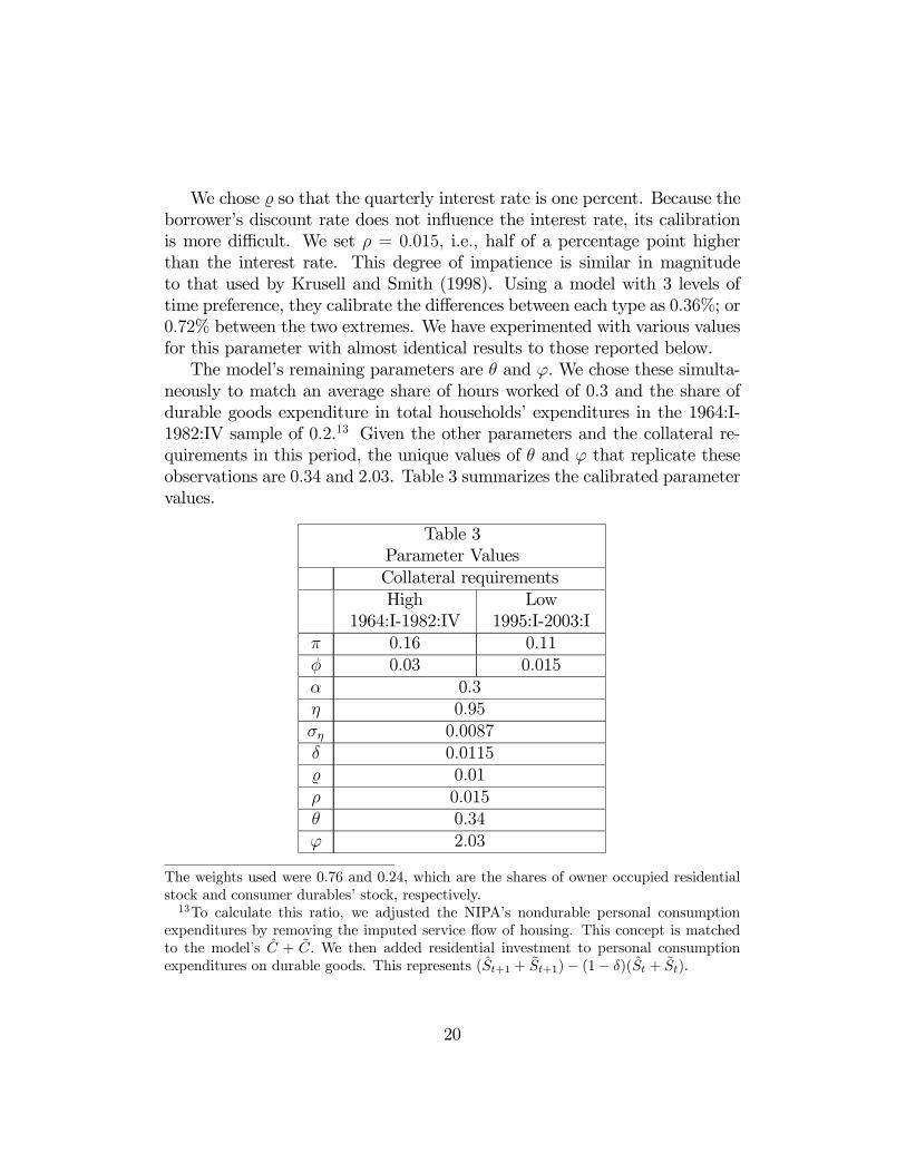
We chose so that the quarterly interest rate is one percent. Because theborrower’s discount rate does not influence the interest rate, its calibrationis more difficult. We set ρ = 0.015, i.e., half of a percentage point higherthan the interest rate. This degree of impatience is similar in magnitudeto that used by Krusell and Smith (1998). Using a model with 3 levels oftime preference, they calibrate the differences between each type as 0.36%; or0.72% between the two extremes. We have experimented with various valuesfor this parameter with almost identical results to those reported below.The model’s remaining parameters are θ and ϕ. We chose these simulta-

neously to match an average share of hours worked of 0.3 and the share ofdurable goods expenditure in total households’ expenditures in the 1964:I-1982:IV sample of 0.2.13 Given the other parameters and the collateral re-quirements in this period, the unique values of θ and ϕ that replicate theseobservations are 0.34 and 2.03. Table 3 summarizes the calibrated parametervalues.

Table 3Parameter ValuesCollateral requirementsHigh

1964:I-1982:IVLow

1995:I-2003:Iπ 0.16 0.11φ 0.03 0.015α 0.3η 0.95ση 0.0087δ 0.0115

0.01ρ 0.015θ 0.34ϕ 2.03

The weights used were 0.76 and 0.24, which are the shares of owner occupied residentialstock and consumer durables’ stock, respectively.13To calculate this ratio, we adjusted the NIPA’s nondurable personal consumption

expenditures by removing the imputed service flow of housing. This concept is matchedto the model’s C + C. We then added residential investment to personal consumptionexpenditures on durable goods. This represents (St+1 + St+1)− (1− δ)(St + St).

20

7.2 Household Borrowing and Aggregate Dynamics

To illustrate how the model works, and in particular the dynamic behavior ofhousehold debt, we consider first the evolution of the two households’ deci-sions in general equilibrium, with the model calibrated to the high collateralregime. Figure 6 plots impulse responses of the two households’ nondurableand durable consumption, the borrower’s hours worked and debt to a posi-tive productivity shock of 1/ (1− α) percent. All the variables are expressedas percent deviations from their steady-state values.The price responses are not shown since they are similar to those in the

standard model. The technology shock directly shifts up labor demand, sothe wage sharply rises and falls slowly to its steady-state level. The interestrate response has a similar shape, given the increased demand for consump-tion by both households, but it is very small given high interest sensitivityof both households.The individual households’ responses to the technology shock strongly

reflect the intertemporal exchange between them. Although the technologyshock increases the rental price of capital and thereby the saver’s income,her durable purchases and nondurable consumption reflect the higher inter-est rate: durable consumption declines and nondurable consumption trendsupwards. The saver’s main reaction to the interest rate is to save by purchas-ing household debt. Thereby, she helps to finance a surge in the borrower’sconsumption. As in the partial equilibrium discussion in Section 6, the in-crease in hours worked by the borrower reflects partial collateral: Laborsupply has to increase to finance durable purchases.A peculiar characteristic of the borrower’s behavior is that temporarily

higher income induces the borrower to increase his debt–in sharp contrastwith the response of a household in a standard model, or the saver in thismodel. The reason for this behavior is that impatience is assumed to beimportant enough for the collateral constraint to bind at all times. Hence,borrowing cannot be a vehicle for consumption smoothing. It is a componentof the transaction of purchasing a durable good.

7.3 Collateral Requirements and Aggregate Volatility

Now we turn to the main issue in the paper: How important is the relaxationof the collateral constraints for aggregate dynamics? Figure 7 compares theimpulse responses of the aggregate variables under the two regimes, high and

21

low collateral constraints, to the same 1/ (1− α) percent increase in At.In the low collateral regime, the responses of hours worked and the debt

are of about half the magnitude of the responses in the high collateral regime.The response of hours worked reflects the mechanism discussed in Section 6:Moving closer to full collateral reduces the labor supply reaction to wagechanges. The change in the response of the debt reflects mainly the declinein the repayment rate φ. When φ > δ, a young durable good has morecollateral value than an old good. Given that the borrower fully exploits thiscollateral value, a positive shock that raises durable purchases increases thedebt even more. Over time, as the average age of the durable goods returns tothe steady-state, the debt converges to its long-run value. This overshootingis eliminated when φ = δ, because age is irrelevant for the collateral value ofa durable good. Lowering the collateral constraint makes φ much closer toδ, and thus the overshooting of the debt is greatly reduced. The response ofdurable expenditures declines.The large proportional decline in the response of hours worked, however,

is translated into a small decline in the response of output, as shown in Figure7. The reason is that given the standard utility and production functions, theresponse of hours worked is small, and hence output dynamics are dictatedprimarily by the exogenous productivity shock. In the next subsection wefollow King and Rebelo (2000) and introduce preferences and productionpossibilities that enhance the contribution of labor fluctuations to output,and thereby reduce the exogenous variation of the shocks that is necessaryto match the volatility of output to the data.

7.4 Collateral Requirements and Aggregate Volatilityin a High-Substitution Economy

Here we adopt both Hansen’s (1985) utility function and a production func-tion with variable capital utilization. The borrower’s utility function is now

E

" ∞Xt=0

e−ρt³θ ln St + (1− θ) ln Ct + γ(1− Nt

´#,

22

where 0 < θ < 1 and γ > 0.14 For the saver, there is no labor supply decision,so that the utility function remains the same.The production structure is changed so as to increase the elasticity of

output with respect to labor without changing the income shares of borrowersand savers. Assume that the production function is now

Yt = (MtK)α (AtNt)

1−α , 0 < α < 1,

where Mt is the composite

Mt =

µZ 1

0

M (i)ζt di

¶1/ζ, 0 < ζ < 1,

of intermediate materials required for capital utilization. Each of these ma-terials is purchased from a profit-maximizing monopoly that produces at theconstant marginal cost. Savers own all the shares in these monopolies.It can be shown that the optimal level of capital utilization is proportional

to output, and thus the production function, solved for capital utilization,can then be expressed as

Yt = κAtNt,

where κ is a constant depending on K, α and the marginal cost of producingM. The elasticity of output with respect to labor is now unity, and thusthere is no return to the ownership of K. However, labor’s share in incomeis not one because the saver receives monopoly profits. These profits are thedifference between total payments to the monopolies and their productioncosts. It can be shown that the share of savers and borrowers in income are,respectively, ν = α (1− α) /(1− α2) and 1− ν = (1− α) /(1− α2).Given that in this economy the capital share is ν, we now calibrate this

parameter, and not α, as 0.3. Also the parameter ση is recalibrated. As forthe basic economy, the criterion is that the simulated standard deviation ofoutput in the high collateral regime equals the standard deviation of output inthe 1964:I-1982:4 period. Given the high-substitution nature of this economy,this parameter is now reduced from 0.0087 in the baseline economy to 0.0038.Figure 8 shows the impulse responses for the two regimes in this economy.

Here, the difference between the high and the low collateral regimes are much

14For computational purposes, we actually use the form θ ln St + (1− θ) ln Ct +

γ(1−Nt)

1−χ

1−χ , with a very small value for χ.

23

more pronounced on impact than for the baseline economy, and somewhatlarger later on.Table 4 presents the standard deviations of HP-filtered data from both

economies. The standard deviations for the baseline economy reflect theimpulse response functions in Figure 7: The decline in volatility is not broadbased. It is concentrated in debt and hours.The results are substantially different for the high-substitution economy,

on which we focus from now on. For labor, the ratio of the standard deviationin the low-collateral regime to its high-collateral counterpart is 0.41. This isclose to the ratio of standard deviations from the periods 1995:I-2003:I and1964:I-1982:IV in Table 1, 0.39. For output, the corresponding ratios fromthe model and data are 0.69 and 0.47. Hence, the mechanism we study canreproduce a large part of the decline in output’s volatility. The same holdsfor the volatility of the debt: the standard-deviation ratio in the model is0.38 and in the data is 0.24.The model does less well in accounting for the behavior of durable goods.

The ratio of standard deviations from the low- and high-collateral regimesis 0.56. The actual ratios for residential investment and durable consump-tion purchases are 0.18 and 0.37. The model’s most counterfactual result isthe small decline in the volatility of nondurable consumption–the standarddeviation ratio is 0.92. The actual volatility ratio is 0.46.The decline in the correlation of hours worked with the debt, which is

very strong in the data–as shown in Table 2–is much weaker in the model.Here, the responses of both variables to shocks are weaker in the low collateralregime, but not very different in shape than in the high collateral regime. Thereason for this result is that the present framework has only one shock. Ifother unrelated disturbances were also included–which do not generate apositive comovement of hours with the debt–weakening the strength of thepresent mechanism would lead to a weaker correlation of hours and the debt.

24

Table 4Model Second Moments

Percent Standard Deviations of HP-Filtered DataBaseline Economy High-Substitution EconomyHigh

CollateralLow

CollateralHigh

CollateralLow

CollateralDebt 2.08 0.95 1.94 0.73Hours Worked 0.56 0.28 1.16 0.47Nondurable Consumption 0.90 0.95 0.73 0.67Durable Purchases 6.31 4.93 7.30 4.11Output 1.97 1.77 1.97 1.36

7.5 Comparison of Level Changes

Figures 1, 4 and 5 indicate that the increase in the debt/durable stock ratiofollowing the reforms in the early 1980s seems to coincide with the trendchange in hours worked per capita. The analysis in Section 5 predicts qual-itatively that both hours worked and the debt/durable stock ratio shouldincrease following a relaxation of the collateral constraints. Here, using theparameter values and the model’s steady state, we can evaluate quantita-tively these changes and compare them to the actual changes of the averagesin the period 1964:I-1982:IV to the averages in the 1995:I-2003:I period.The actual percentage increase in hours per-capita across these two pe-

riods is 11.1%. In the baseline economy, the steady state increase from thehigh to the low collateral regime is 5.3%, and in the high-substitution econ-omy it is 7.7%. Regarding the debt/durable stock ratio, the average ratiofor the period 1964:I-1982:IV is 0.35. For 1995:I-2003:I it is 0.47. In the twomodel economies, the ratio from the high collateral regime is 0.21. Changingto the low collateral regime raises this to 0.42.

8 Links with the Literature

This paper follows Krusell and Smith (1998) in studying the cyclical interac-tion of agents having heterogeneous thrift attitudes in an environment withborrowing constraints. Krusell and Smith stress in particular the role of con-straints on non-collateralized borrowing for the cyclical behavior of savingand investment. They use a setup where the rate of time preference is sto-

25

chastic, although persistent, so that “borrowers” and “savers” interchangeat some point. Beyond the different modelling strategy, the main departureof our analysis from theirs is the introduction of household durables andcollateralized debt, and the interaction with labor supply. The key role ofdurables in this context was stressed in Section 6: If all consumption goodsare nondurable, the agents who supply labor may not vary hours worked overthe business cycle at all.The different rates of time preference in a two-agents setup as the present

one are endogenous in Gomme and Greenwood (1995), as negative functionsof wealth accumulation. Possibly, adopting that specification could generatea setup similar to the current one as the limit of a process starting from identi-cal agents and a one-time perturbation in income–that triggers increasinglydifferent rates of time preference and wealth.Microeconomic evidence supporting the notion that collateral constraints

tie together labor supply and household debt include Fortin (1995) and DelBoca and Lusardi (2003). Using Canadian and Italian data, they foundthat labor participation of married women increases with their households’mortgage debt.The possible implications of financial market innovations for the decline

of macroeconomic volatility in the early 1980s were discussed by Blanchardand Simon (2001) and Stock and Watson (2002, 2003). Blanchard and Simonpoint out that an enhanced ability of smoothing consumption due to financialinnovations does not seem a promising route for explaining the greater macro-economic stability: One would expect these developments both to reduce thevolatility of nondurable consumption and services and to increase the volatil-ity of durable purchases–due to easier adjustment to optimal stocks. How-ever, in the early 1980s the volatility of the three components of consumptiondeclines, and to a similar degree. Stock and Watson stress the innovationsin the mortgage market in particular, and the observed drastic decline inthe volatility of residential investment in the early 1980s, among one of thepossible sources of the increased macroeconomic stability since then. This isthe direction adopted in this paper.Kiyotaki and Moore (1997) focused on the cyclical implications of collat-

eral constraints on firms. In their analysis, productive capital serves a dualrole, as collateral for loans and in production. In the present paper, durablegoods play a dual role for households, as collateral for loans and in utility.Both setups generate endogenous transmission of shocks, but the mechanismsare very different. In Kiyotaki and Moore, an exogenous shock that increases

26

investment of a credit-constrained firm is transmitted to further investmentdue to the additional collateral obtained. Here, an exogenous shock thatincreases income of a credit-constrained household is magnified by a laborsupply effect, but only under partial collateral–with full collateral, the laborsupply response disappears.The cyclical interaction of home durables with hours worked was also

addressed from a home production perspective, as, for example, in Rupert,Rogerson and Wright (2000) and Fisher (2001). In these models, which in-corporate perfect capital markets, the interaction between the two variablesdepends on the technological role assigned to home capital. Rupert, Roger-son and Wright point out that home production by itself should not generatea link between home capital and labor supply under perfect capital mar-kets. Fisher incorporates a mechanism by which home capital improves theeffectiveness of hours worked in the market, and thus generates a positivecomovement between household capital and labor supply. The long-run re-lationship between home durables and labor participation was analyzed byGreenwood, Seshadri and Yorukoglu (2003). In their model, the adoptionof new home durables substitutes labor in home activities, and thus induceshigher participation in market production.

9 Concluding Remarks

The present mechanism of relaxing the collateral constraints on householdsseems quantitatively important for explaining the decline in macroenomicvolatility since the early 1980s. This framework is consistent with differentaspects of actual behavior of household debt and other key macroeconomicvariables, particularly labor and output. Aggregate volatility declines as thelevel of household debt and hours worked start to increase after the financialreforms of 1982.The present analysis could be extended in different directions. One ex-

ample is a cross-country comparison that exploits different features of thehousehold credit markets. This model could also prove useful for the analysisof fiscal issues, such as the macroeconomic implications of mortgage interestdeductions from income tax, or optimal taxation of capital and labor.In general, the model presented here is a tractable alternative to the

representative-agent framework for macroeconomic analysis, and it seemsparticularly appropriate for the analysis of issues involving the credit market.

27

References

[1] Aizcorbe, Ana M., Arthur B. Kennickell, and Kevin B. Moore, 2003,“Recent Changes in U.S. Family Finances: Evidence from the 1998 and2001 Survey of Consumer Finances,” Federal Reserve Bulletin, 89, 1-32.

[2] Blanchard, Olivier, and John Simon, 2001, “The Long and Large Declinein U.S. Output Volatility,” Brookings Papers on Economic Activity, 135-164.

[3] Del Boca, Daniela, and Annamaria Lusardi, 2003, “Credit Market Con-straints and Labor Market Decisions,” Labour Economics, 681-703.

[4] Fisher, Jonas D. M., 2001, “A Real Explanation for Heterogenous In-vestment Dynamics,” Federal Reserve Bank of Chicago working paper.

[5] Florida, Richard, L. 1986, “Housing and the New Financial Markets,”Rutgers-The State University of New Jersey.

[6] Fortin, Nicole, M., 1995, “Allocation Inflexibilities, Female Labor Sup-ply, and Housing Assets Accumulation: Are Women Working to Pay theMortgage?,” Journal of Labor Economics, 13, 524-557.

[7] Gomme, Paul, and Jeremy Greenwood, 1995, “On the Cyclical Alloca-tion of Risk,” Journal of Economic Dynamics and Control, 19, 91-124.

[8] Greenwood, Jeremy, Seshadri, Ananth and Mehmet Yorukoglu, 2003,“Engines of Liberation,” forthcoming in theReview of Economic Studies.

[9] Hansen, Gary D, 1985, “Indivisible Labor and the Business Cycle,” Jour-nal of Monetary Economics, 16, 309-327.

[10] Hansen, Gary D., and Edward C. Prescott, 2001, “Capacity Constraints,Asymmetries, and the Business Cycle,” manuscript.

[11] Kahn, James, Margaret M. McConnell, and Gabriel Perez-Quiros, 2002,“On the Causes of the Increased Stability of the U.S. Economy,” FederalReserve Bank of New York Economic Policy Review, 8, 183-202.

[12] King, Robert, G., Charles I. Plosser and Sergio T. Rebelo, 1988, “Pro-duction, Growth and Business Cycles I.” Journal of Monetary Eco-nomics, 21, 195-232.

28

[13] King, Robert G., and Sergio T. Rebelo, 2000, “Resuscitating Real Busi-ness Cycles,” in John Taylor and Michael Woodford (eds) Handbook ofMacroeconomics, North Holland, 927-1007.

[14] Kiyotaki, Nobuhiro, and John Moore, 1997, “Credit Cycles,” Journal ofPolitical Economy, 105, 211-248.

[15] Krusell, Per, and Anthony A. Smith, Jr., 1998, “Income and WealthHeterogeneity in theMacroeconomy,” Journal of Political Economy, 106,867-896.

[16] McConnell, Margaret. M., and Gabriel Perez-Quiros, 2000, “OutputFluctuations in the United States: What Has Changed Since the Early1980s,” American Economic Review, 90, 1464-1476.

[17] Olney, Martha, L., 1991, “Buy Now Pay Later,” The University of NorthCarolina Press.

[18] Projector, Dorothy S., and Gertrude S. Weiss, 1966, “Survey of Finan-cial Characteristics of Consumers,” Federal Reserve Technical Papers,August.

[19] Rupert, Peter, Rogerson, Richard, and Randall Wright, 2000, “Home-work in Labor Economics: Household Production and IntertemporalSubstitution,” Journal of Monetary Economics, 46, 557-579.

[20] Semer, Milton P., Julian H. Zimmerman, John M. Frantz and AshleyFord, 1986, “Evolution of Federal Legislative Policy in Housing: HousingCredits,” in Richard L. Florida (ed.) Housing and the New FinancialMarkets, Rutgers-The State University of New Jersey.

[21] Stock, James H., and Mark W. Watson, 2002, “Has the Business CycleChanged and Why?,” NBER Macroeconomics Annual, 159-218.

[22] Stock, James H., and Mark W. Watson, 2003, “Has the Business CycleChanged? Evidence and Explanations,” manuscript.

29

.28

.32

.36

.40

.44

.48

65 70 75 80 85 90 95 00

Ratios of Household Debt to Durable Goods

Total Debt/Total Stock

Mortgage Debt/Residential Stock

Figure 1

30

-.08

-.06

-.04

-.02

.00

.02

.04

.06

.08

65 70 75 80 85 90 95 00

Hours

Debt

Household Debt and Hours WorkedHP-filtered

Figure 2

-.08

-.06

-.04

-.02

.00

.02

.04

.06

65 70 75 80 85 90 95 00

Debt

Hours

Mortgage Debt and Hours WorkedHP-filtered

Figure 3

31

5

10

15

20

25

30

35

0.85

0.90

0.95

1.00

1.05

1.10

65 70 75 80 85 90 95 00

Household Debt and Hours Worked

Deb

t per

Cap

ita (t

ens

of th

ousa

nds

of 2

000

dolla

rs)

Hours per C

apita (Index)

HoursDebt

Figure 4

5

10

15

20

25

0.85

0.90

0.95

1.00

1.05

1.10

65 70 75 80 85 90 95 00

Mortgage Debt and Hours Worked

Hours per C

apita (Index)D

ebt p

er C

apita

(ten

s of

thou

sand

s of

200

0 do

llars

)

Hours

Debt

Figure 5

32

0 4

812

1620

0

0.250.5

Hou

rs W

orke

d

0 4

812

1620

0

0.51

1.5

Deb

t

04

812

1620

-0.50

0.5

Bor

row

er's

Dur

able

Con

sum

ptio

n

04

812

1620

-0.50

0.5

Sav

er's

Dur

able

Con

sum

ptio

n

04

812

1620

0

0.2

0.4

0.6

0.8B

orro

wer

's N

ondu

rabl

e C

onsu

mpt

ion

04

812

1620

0

0.2

0.4

0.6

0.8

Sav

er's

Non

dura

ble

Con

sum

ptio

n

04

812

1620

0

0.2

0.4

Hou

rs W

orke

d

04

812

1620

0

0.51

1.5

Deb

t

04

812

1620

0

0.2

0.4

0.6

Non

dura

ble

Con

sum

ptio

n

04

812

1620

024

Dur

able

Con

sum

ptio

n E

xpen

ditu

res

04

812

1620

0.51

1.5

Out

put

Hig

h C

olla

tera

l Reg

ime

Low

Col

late

ral R

egim

e

04

812

1620

0123H

ours

Wor

ked

04

812

1620

0123D

ebt

04

812

1620

0.4

0.6

0.81

Non

dura

ble

Con

sum

ptio

n

04

812

1620

051015D

urab

le C

onsu

mpt

ion

Exp

endi

ture

s

04

812

1620

024O

utpu

t

Hig

h C

olla

tera

l Reg

ime

Low

Col

late

ral R

egim

e