Embed Size (px)
Citation preview

DI
SC
US
SI
ON
P
AP
ER
S
ER
IE
S
Forschungsinstitut zur Zukunft der ArbeitInstitute for the Study of Labor
The Role of Demographics in Precipitating Crises in Financial Institutions
IZA DP No. 4436
September 2009
Diane J. Macunovich

The Role of Demographics in Precipitating
Crises in Financial Institutions
Diane J. Macunovich University of Redlands
and IZA
Discussion Paper No. 4436 September 2009
IZA
P.O. Box 7240 53072 Bonn
Germany
Phone: +49-228-3894-0 Fax: +49-228-3894-180
E-mail: [email protected]
Any opinions expressed here are those of the author(s) and not those of IZA. Research published in this series may include views on policy, but the institute itself takes no institutional policy positions. The Institute for the Study of Labor (IZA) in Bonn is a local and virtual international research center and a place of communication between science, politics and business. IZA is an independent nonprofit organization supported by Deutsche Post Foundation. The center is associated with the University of Bonn and offers a stimulating research environment through its international network, workshops and conferences, data service, project support, research visits and doctoral program. IZA engages in (i) original and internationally competitive research in all fields of labor economics, (ii) development of policy concepts, and (iii) dissemination of research results and concepts to the interested public. IZA Discussion Papers often represent preliminary work and are circulated to encourage discussion. Citation of such a paper should account for its provisional character. A revised version may be available directly from the author.

IZA Discussion Paper No. 4436 September 2009
ABSTRACT
The Role of Demographics in Precipitating Crises in Financial Institutions
There are significant effects of changing demographics on economic indicators: growth in GDP especially, but also the current account balance and gross capital formation. The 15-24 age group appears to be one of the key age groups in these effects, with increases in that age group exerting strong positive effects on GDP growth, and negative effects on the CAB and GCF. There have been major shifts in the share of the population aged 15-24 during the past half century or more, many of which correspond closely to periods of institutional turmoil. The hypothesis presented in this paper is that increases in the share of the 15-24 age group lead producers to ratchet up their production expectations and take out loans to expand production capacity; but then reductions in that share – or even declining rates of increase – confound these expectations and precipitate a downward spiral of missed loan payments and even defaults and bankruptcies, putting pressure on central banks and causing foreign investors to withdraw funds and speculators to unload the local currency. This appears to have been the pattern not only during the 1996-98 crisis with the Asian Tigers, but also during the “Tequila” crisis of the early 1990s, the crises that occurred in the early 1980s among developed as well as developing nations, and the economic problems Japan has experienced since about 1990. The effect appears to be even more pronounced for the current 2008-2009 period. JEL Classification: J1, E3, F3, F4 Keywords: age structure, currency crisis, demographic change, financial crisis Corresponding author: Diane J. Macunovich Department of Economics University of Redlands Redlands, CA 92346 USA E-mail: [email protected]
3
The intention in this paper is to describe an empirical regularity concerning changes in the age structure
of the population – specifically, changes affecting those portions of a country’s population most
responsible, on a per capita basis, for growth in aggregate demand. Historically, in many instances when
financial institutions have experienced crises, there has been a reversal in the rate of growth of those
segments of the population, across a number of countries affected by the crises. That reversal appears to
have been correlated, in turn, with economic slowdowns which may be qualitatively different from those
associated with a normal business cycle. If so, it might suggest an early warning signal provided by
demographic structure established some decades earlier.
The plan in this paper is first to consider the possible role of slowdowns in the growth of aggregate
demand, in triggering institutional crises (section I); set out the demographic argument central to this
paper (section II); discuss the potential significance of demographics in economic activity generally
(section III); explore empirically the relationship between demographics and indicators of economic
activity (section IV); and then finally to illustrate the demographic changes that have occurred
simultaneously with crises (section V).
I. The Role of Aggregate Demand in Institutional Crises
In 1997 and 1998 the “Asian Tigers” -- Indonesia, Korea, Malaysia, the Philippines and Thailand --
experienced a sharp drop in the value of their currencies and a reversal of private capital flows from
abroad. Whereas foreign investors had been pouring massive amounts of capital into these countries prior
to 1997, they began to withdraw funds at an even faster rate after June of 1997, severely depressing
economic indicators and even in some cases creating political turmoil. There was a similar type of
occurrence among Latin American countries earlier in the 1990s (often referred to as the “Tequila” crisis),
and in Chile in 1982. The literature abounds with analyses and models put forward to explain these
phenomena, but all of them tend to focus on financial and policy aspects of the upheavals, without

4
seeming to consider whether the episodes might have been demand driven. The words “population” and
“demographics” are conspicuously absent from the literature.
It is possible to insert demographics into the various models without actually altering them. We just need
to recognize the demographic factors at work behind the mechanisms outlined in those models. To see
this, we need to consider the two primary models which have emerged from the literature. The first
focuses on macroeconomic fundamentals, such as the current account balance, international capital flows,
the exchange rate and interest rates, and finds unsustainable imbalances and problematic government
policies. This model sees a central bank attempting to defend its exchange rate -- and thus drawing down
its foreign reserves -- while at the same time finding it necessary to shore up and then ultimately bail out
banks and other financial institutions that begin failing under the pressure of increasing numbers of non-
performing loans -- loans which had been made at breakneck rates in the previous years. Speculators
attack the currency, and foreign investors call in loans, in anticipation of an exchange rate devaluation.
This is what occurs in a country
"whose private sector is subject to a series of shocks that threaten corporate and banking profitability. These financial difficulties may require the government to bail out troubled institutions. . .Agents observing the weaknesses of the private sector can see that the government will be forced to adopt an expansionary monetary stance in the future to finance the costs of bailout intervention. Since such expansion is inconsistent with maintaining the exchange rate peg, investors will expect the currency to depreciate, and this expectation will trigger a speculative attack. (Pesenti & Tille, 2000:4-5)
The second model is closely related – so much so that Pesenti and Tille (2000) argue that the two are
actually complementary – but focuses on the role of speculators in creating a self-fulfilling crisis. That is,
in anticipation of a possible exchange rate devaluation, speculators unload the local currency, thus
drawing down foreign reserves and ultimately forcing the government to actually devalue. Pesenti and
Tille present a model of contagion in which
“A currency depreciation in one country weakens fundamentals in other countries by reducing the competitiveness of their exports. . .initial turmoil in one country can lead outside creditors to recall their loans elsewhere.”

5
“. . .a currency crisis in one country can worsen market participants' perception of economic outlook in countries with similar characteristics.”
And this idea of contagion can also apply within a country, spreading the effects of bankruptcy:
“Debt rollover difficulties, even when located in one sector of the economy, can spill over the whole economy and result in vanishing credit and a major welfare loss. (Calvo, 2000:91)
However, as Calvo (2000) points out, none of the models explain why the crises happened when they did:
Without question, there were macroeconomic imbalances, weak financial institutions, widespread corruption, and inadequate legal foundations in each of the affected countries. These problems needed attention and correction, and they clearly contributed to the vulnerability of the Asian economies. However, most of these problems had been well known for years. . .(Calvo, 2000:150)
The focus here is on those bankruptcies and non-performing loans mentioned earlier. They could well be
the result of a slowing economy: investors who had counted on continuing economic growth to generate
revenues, are caught when growth slows and revenue streams fall short of those anticipated. Similarly,
“[c]ontinuing and in some cases increasing, high economic growth gave confidence to foreign investors”
(Calvo, 2000:117) prior to 1997 -- but seeing revenue streams drying up with a slowdown, they withdrew
their funds. There is evidence of slowdowns:
A stylized fact . . .is that output and consumption growth the year of the crisis are lower than the averages in the three preceding years. . .( Milesi-Ferretti & Razin, 2000 )
Among the Asian Tigers, the first indicator that a problem might exist was the bankruptcy of three major
companies in Korea, in January of 1997 – Hanbo Steel, Sammi Steel and Kia Motors -- and payments on
its foreign debt were missed by Samprasong Land in Thailand (Calvo, 2000:134-5). This was
accompanied by a general fall in property markets, and increasing numbers of non-performing loans.
This picture, of demand-driven crisis, seems to be supported by some:
“Speculative attacks leading to currency crises can follow a collapse in domestic asset markets (as seems to have been the case recently in Asia). . .”(Milesi-Ferretti & Razin, 2000:286
6
“. . .microeconomic indicators (such as corporate profitability and debt-to-equity ratios) can help predict the imminence and the likelihood of a currency crisis better than the standard macroeconomic indicators (such as fiscal imbalances and current account deficits).” (Pesenti & Tille, 2000:7)
However, much of the literature seems to assume that any slowdown was a result of the crisis, rather than
its cause:
“. . .the experience of emerging economies has suggested to many that currency crises, by forcing these countries to move suddenly from current account deficit to surplus, cause severe economic downturns.”(Krugman, 2000:5) “. . .currency crashes are normally associate with sharp declines in output.” (Krugman, 2000:5) “Recent financial crises in emerging markets have shared the following characteristics. . .(4) They led to a sharp growth slowdown, if not sheer output collapse.” (Calvo, 2000:71) “Output loss can be rationalized in terms of "new classical" and price-stickiness models: in the first one because a crisis changes relative prices and may cause a generalized financial crash and in the second one for textbook-type Keynesian reasons associated with a contraction of aggregate demand.” (Calvo, 2000:72)
II. The Argument Put Forward in This Paper
The assumption in this paper is that the slowdown led to the bankruptcies and subsequent lack of
confidence among investors -- and that the slowdown itself was generated at least in part by demographic
changes. The argument hinges on the notion that a significant portion of the growth in demand in the
economy comes from new household formation. Some of this new household formation will result from
immigration, but the vast majority of it results from young adults leaving their parents’ homes and
forming their own households. They generate demand for housing and consumer durables including
automobiles. If there is growth in this segment of the population, there will be overall growth in
consumption, and similarly rates of growth in consumption will fall with declines in the growth rate of
this significant group.

7
This group's expenditures do not appear significant in Consumer Expenditure Surveys (CES) such as
those conducted by the Bureau of Labor Statistics in the U.S., but shelter costs are represented there only
in terms of interest or rental payments, not total expenditure. (Expenditures on house purchase appear as
changes in total assets and liabilities.) Thus the actual total expenditure generated in the economy by the
age group in providing new housing units – whether rental or owned – is not represented as expenditure in
the CES. This effect is magnified by the fact that a good deal of expenditure on cars, housing, and
furnishings for the group is often made by parents, and reported as expenditure by the parental age group
rather than by the target age group. The only way to see the total impact of this or any age group is to
analyze econometrically the relationship between the growth in various age group shares, and growth in
GDP per capita.
Consider a representative producer: demand for his product has been growing steadily for several years
now, and in the manner of most analysts, his marketing people have simply extrapolated that pattern of
growth into the future, suggesting that he should be expanding his production capacity. He takes out a
loan to finance a plant expansion, and contracts with suppliers for continually increasing amounts of
input, attempting to build up an inventory in anticipation of future sales. But then fairly suddenly the rate
of growth in demand slows – or even turns negative – and he finds himself with significant over-capacity
and heavy loan payments. He cancels contracts with suppliers – thus causing his own slowdown to
snowball down through the supply chain – and begins to miss loan payments. Then he finds himself, like
Hanbo Steel, in bankruptcy. The problem was not so much the slowing growth, as his expectations of
increasing growth, which led him to plan for expansion that later could not be supported.
“Of the components of aggregate demand, it is the investment spending by firms and households that is the prime mover in economic fluctuations, being by far the most cyclical and the most volatile. . .If an economic slowdown reduces profit margins and dims the outlook for profits, the likely reaction of business firms will consist first in cutbacks on decisions to invest, then if matters do not improve, in reductions of inventories, output and employment.” (Victor Zarnowitz, 1999:73-74)

8
If this happens throughout the economy, it could well lead to the economic scenario described by the
crisis models, as banks become pressured by non-performing loans and find themselves unable to pay
foreign creditors. All because of faulty expectations and a shift in the population age structure.
III. The Role of Demographics in Economic Activity
An earlier study (Macunovich, 2007) demonstrated a strong age-related pattern of consumption using
state-level personal consumption expenditure data, and population by single year of age, for the U.S. from
1900 through 1987. That work suggested that the passage of the U.S. baby boom from childhood through
the teen years and into family formation caused marked swings in patterns of aggregate consumption
demand in the United States during the second half of the twentieth century. Applying that study’s
estimated age-group effects to time trends of national U.S. population age structure suggested that,
holding other factors constant (including income and total population size), the baby boom-generated
changes in age structure accounted for swings of about 25% in total real aggregate personal consumption
demand.
Similarly, Fair and Dominguez (1991) found significant effects of detailed age structure in the adult
population, on all forms of consumption demand in the U.S., including housing demand, and on the
demand for money.
A strong differential effect of specific age groups on economic performance has also been demonstrated
in the work of Jeffrey Williamson and his colleagues, using the “Asian Tigers” and also the pre-1914
Atlantic economy1. They have shown that the proportion of children relative to working age adults has
dramatic effects on savings rates and the demand for capital – and hence on foreign capital dependence.
Like the findings in Macunovich (2007), but unlike those of Fair and Dominguez (who looked only at age
1 Bloom and Williamson (1998), Higgins and Williamson (1997) and Higgins (1998)

9
structure among adults), the work of Williamson and colleagues addressed distributional effects using
detailed age breakdowns throughout the entire age structure, including children, finding a negative effect
of population growth per se, but a positive effect of the proportion of the population in the prime working
ages. They attribute much of the “Asian miracle” – and of pre-1914 growth in the Western world – to the
entry into prime working ages of these countries’ “baby boomers” – the population swell produced during
their respective demographic transitions.
Four other papers look at the effect of changing age structure on economic growth as well. Della Vigna
and Pollet (2007) find a strong effect on industry portfolio returns based on long term growth due to
demographics. Feyrer (2007, 2008) examines the effect of demographics on productivity and output per
worker, finding a strong positive effect of the 40-49 age group (but looking only at workers aged 10-69,
rather than at the entire population). Bloom and Finlay (2009), in turn, demonstrate a strong effect of the
working age (15-64) population on economic growth, in terms of income per capita, in thirteen South and
East Asian nations.
Much of the work to date gives credit to changing population age structure, in generating strong economic
growth. But although these researchers allude to growth slowdowns as populations age, they don’t seem
to address the potential for economic turmoil created by the transition from high to low growth in specific
age groups. This is probably because to a great extent their models attribute growth to the entire working-
age population – the 15-64 age group – and any transition in such a large age group’s population share
would be very gradual: barely discernable on a year-to-year basis.
Given the fact that they are forming new households, it seems that changes in the size of the young adult
age group – say, approximately from age 15 to 24 – will have a very different effect on the economy than,
say, changes in the numbers of 55-64 year olds, who are simply existing households passing from one age
10
group to another. To the extent that this is the case, when the 15-24 age group’s share of population
begins to decline, producers will be hit with an unexpected drop in the growth of demand for their
products, leading to inventory build-ups and production cutbacks — as alluded to by J.M.Keynes:
“An increasing population has a very important influence on the demand for capital. Not only does the demand for capital — apart from technical changes and an improved standard of life — increase more or less in proportion to population. But, business expectations being based much more on present than prospective demand, an era of increasing population tends to promote optimism, since demand will in general tend to exceed, rather than fall short of, what was hoped for. Moreover a mistake, resulting in a particular type of capital being in temporary over-supply, is in such conditions rapidly corrected. But in an era of declining population the opposite is true. Demand tends to be below what was expected, and a state of over-supply is less easily corrected. Thus a pessimistic atmosphere may ensue; and, although at long last pessimism may tend to correct itself through its effect on supply, the first result to prosperity of a change-over from an increasing to a declining population may be very disastrous.” (John Maynard Keynes, 1937, emphasis added)
Through a chain reaction of similar types of cutback the economy may tailspin into an economic slump –
as suggested by J.K.Galbraith:
“The bankers yielded to the blithe, optimistic, and immoral mood of the times. . .one failure led to other failures, and these spread with a domino effect” (John Kenneth Galbraith, 1954)
This is not to say that decline in the young adult age group in and of itself is harmful for an economy:
many have argued eloquently against such a notion, even in the case of population decline generally.2
Rather, it is the turning point from rising to falling proportions of young adults that appears to pose a
potential threat to economic stability, and “unexpected” is the key word in the previous paragraph —
again as suggested by Keynes above. Producers can in time accommodate themselves to decline, as long
as it’s expected: it is the unexpected, that occurs at turning points, which “may be very disastrous”
(Keynes, 1937).
2 See, for example, Easterlin (1996).

11
The extent of any institutional turmoil induced by such turning points is undoubtedly a function of many
factors in addition to changes in population age structure — most notably, the integrity of the banking
system, and the financial sector generally, and the ability of the public sector to prevent escalation.
Schumpeter (1946) attributed the virulence of the 1929 crash to “. . . supernormal sensitivity of the
economic system to adverse occurrences and. . . the weaknesses in the institutional setup”. As
international trade has grown and strengthened, the integrity and stability of trade partners has become
significant, as well.
Thus it could be that a relatively small change in the growth rate of the young adult age group in the U.S.
in 1929, when financial systems were less robust, and major trading partners experienced more severe
declines, had significantly greater effects than a much larger change in age structure in 1973, when
monetary and fiscal policies of the government had a more stabilizing influence and most trade partners
had not yet experienced any decline. Unforeseen changes in population age structure have the potential
for triggering catastrophic institutional turmoil — and virtually always appear to cause at least a degree of
economic dislocation.
There appears to be evidence that this process has been at work in the U.S. over the past one hundred
years, as demonstrated in Figure 1. The curve on the graph represents the annual rate of change in the
proportion of young adults in the U.S. population. “Young adults” are defined as those aged 15-19 prior
to 1950, and 20-24 in the years thereafter, given changing levels of educational attainment over time. The
vertical lines mark the start of recessions, as defined by NBER. There is a very close correspondence
between the vertical lines, and peaks in the curve, as well as points where the curve goes negative. In
addition, the deep trough between 1937 and 1958 contained another four recessions, and there were two
in the trough between 1910 and 1920 (not marked on the graph). The only recessions over the last one
hundred years that don’t appear to correspond to features of the curve, are those in 1920, 1926 and 1960.

12
The pattern of causation – if it is one – cannot for the most part run from the economy to demographics,
since these are young people born over 15 years before each economic downturn. To control for the
possibility that the size of the young adult age group might be affected by economically-induced
migration, lagged values of age shares have been used. That is, the graph actually shows the pattern of
change in the 14-18 and 19-23 year age groups, one year earlier. (The pattern is virtually unchanged from
that obtained using unlagged values.)
A similar type of relationship is presented for Japan in Figure 2 (again using lagged values to instrument
the actual rates of change). There it can be seen that Japan experienced a substantial drop in the growth
rate of the 20-24 age group during the period now referred to as its "lost decade".
IV. The Analysis
The goal of this analysis was to test for a significant relationship between macroeconomic variables and
population age shares, at both the national and the international level. The economic data were taken
from an unbalanced panel for approximately 155 countries in the period 1960 through 2004/5, prepared
by the World Bank (2007): annual growth rate of GDP per capita (GDPpc), the Current Account Balance
as a percent of GDP (CAB), and Gross Capital Formation as a percent of GDP (GCF). Summary
statistics for these variables are presented in Table 1. All of the regressions were estimated using Stata’s
cross-sectional time series “xtreg” procedure, with fixed effects.
Rates of growth in population age shares for all countries except the U.S. were calculated from data
prepared by the UN (1999), which provides population in five year age groups for approximately 170
countries from 1950 – 2000, with forecasts to 2050. The U.S. data are for single year age groups, 1900-
1995 and forecast to 2050, provided on diskette by the U.S. Bureau of the Census (1996). Although age

13
groups other than the 0-4 are in large part pre-determined in any current time period, as births which
occurred in earlier periods, there is some possibility of endogeneity in the sense that current economic
conditions might induce immigration or emigration. For this reason, lagged values of the population
variables have been used in all analyses presented in this paper. For example, the change in the share
aged 15-24 in a given year is instrumented using the change in the share of the same cohort five years
earlier (that is, the change in the 10-19 age group five years earlier)
It is important, in such an analysis, to work with fairly small age groupings – to divide the population into
a fairly large number of age groups – in order to allow for effects which may vary significantly, even
between age groups that are fairly close. (Think, for example, of 0-4 year olds as compared with 10-14
year olds. These are typically lumped together in the “dependent” 0-14 age group, and yet their own
behavior – and parental spending on the two groups – can vary significantly.)
Ideally a large number of age groups would be separately identified as independent variables in the
analysis to avoid this age group identification problem. But a model that includes a large number of age
groups in order to overcome the possibility of erroneous groupings, might encounter a problem of severe
multicollinearity that calls into question the accuracy of any individual coefficient estimates. And
problems of multicollinearity are compounded by the marked loss of degrees of freedom in estimating
those coefficients, as the number of age groups is increased — an important consideration in time series
analyses. As observed by David (1962), “Age varies continuously and there are few convenient
demarcations between age groups with significantly different behavior patterns.” Thus we face a
conundrum: construct “artificial” and possibly erroneous age groupings, or face the possibility of severe
multicollinearity among more finely disaggregated groupings.

14
In the first stage of the analysis, in order to minimize problems associated with the identification of
“homogeneous” age groups within the population, detailed age breakdowns of the total population were
used, in a method first implemented by Fair and Dominguez (1991), and used in later analyses by Higgins
and Williamson (1997) and Higgins (1998).3 The Fair-Dominguez method of parameterizing multiple
age groups is based on Almon’s (1965) distributed lag technique. This methodology has subsequently
been adopted in more recent studies, and is described in more detail in the Appendix. In general terms, it
is one that permits the estimation of coefficients on single year population age shares by constraining
those coefficients to lie along a polynomial. The coefficients φj on J population age shares pj are assumed
to enter the consumption equation in the form
j
J
jj p∑
=1
ϕ (1)
which is estimated as a polynomial
nnj
J
jj ZZZp ςςςϕ +++=∑
=
…22111
(2)
in which n is the degree of the polynomial and
∑∑∑===
−=J
j
nJ
jj
nJ
jjn jpJjpZ
111
/1 (3)
Each Z that results from this procedure is essentially a summation of weighted population age shares. In
the first variable, Z1, the age weights are raised to the first power, while in Z2 they are squared, and then
in Z3 they are cubed, and so on. In the regression results, the estimated coefficients on the individual
population age shares can be easily recovered from the coefficients estimated for the Z’s.
3 It must be emphasized that the inclusion of the full age distribution – including infants and children – in a more aggregated model does not in any way imply or necessitate decision-making on the part of children themselves, with regard to their patterns of consumption. It simply allows for the fact that children in one household might affect the spending patterns of individuals in other age groups and/or households.

15
Determining the degree of the polynomial, n – the number of these population age Z’s to include as
explanatory variables – appears in earlier studies to have been based largely on economic theory,
assuming a quadratic at the aggregate level based on the hypothesized life cycle “hump-shaped” pattern at
the micro level. (That is, using just two Z’s, Z1 and Z2.) But as emphasized earlier in this paper, because
of inter-household effects a different pattern may emerge at the aggregate level, and this pattern might
vary across cultures, depending on, for example, the role of children in society, the age at which young
people leave their parents’ homes, and whether the government provides any form of financial support in
old age.
There is more danger in under- than in over-estimating the degree of the polynomial. Judge et al
(1985:359-60) state that while overestimates of the true degree of the polynomial produce estimators that
are unbiased but inefficient, underestimates of the true degree produce estimates that are “always biased”.
For this reason, they suggest starting with a higher level than is assumed to apply in the true model and
stepping down, testing each additional restriction and finally accepting the level that “produces the last
acceptable hypothesis [their italics]”. That procedure has been adopted in this study, beginning with n=9
and working down until a regression produces significant coefficients on the highest Z amalgams.
This technique was applied to four groups of countries:
- all countries taken together
- the "Asian Tigers" that experienced a financial crisis in the 1996-98 period: Korea, Indonesia,
Malaysia, Philippines and Thailand
- the "Tequila Group" that experienced a financial crisis in the 1992-1994 period: Mexico. Brazil,
Argentina, Colombia and Peru
- the USA and Japan

16
In this way it was determined that n=6 for the “Asian Tigers” regression, n= 3 for the Tequila Group, and
n=7 for the other two groups. Table 2 and Figure 3 present the results of this first stage of the analysis,
using the Fair-Dominguez methodology.
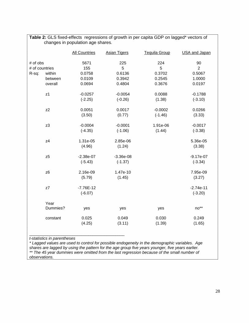
Table 2 presents the results of regressing the rate of growth in per capita GDP on lagged rates of growth
in population age shares, as represented using the Z’s. There it can be seen that all coefficients are
significant for "All Countries" and for the USA and Japan, while the highest Z's are significant at about
the 0.15 level for the Asian Tigers and the Tequila Group. In Figure 3, the age share coefficients have
been recovered from the coefficients on the Z’s and are displayed for each of the four country groups.
Although at first glance the shapes in the four graphs in Figure 3 might appear quite different, upon closer
examination it can be seen that there is a striking similarity among the four, in terms of the effect of
children under 15 (negative), and young adults aged 15-24 (positive -- marked by the two vertical bars).
In addition, there is also a positive effect of middle-aged groups in all but the Tequila Group, where the
third degree polynomial of the regression does not permit a finer demarcation of age groups. The positive
effect of the middle-aged groups is consistent with findings in studies mentioned earlier4. These earlier
studies do not specifically examine the 15-24 age group, however. The significant positive effect of the
15-24 age group estimated here is consistent with the hypothesis stated in earlier sections: that growth in
the share of young adults in the household formation stage, between ages 15 and 24, will tend to have a
very strong positive effect on growth in consumption, as they set up and furnish their own homes, buy
cars, and start families.
The effects of older age groups on the growth rate of per capita GDP are noteworthy. While the oldest
age groups exert a negative influence for the Asian Tigers, the Tequila Group and the USA and Japan, 4 Bloom and Williamson (1998), Higgins and Williamson (1997), Higgins (1998), Feyrer (2007, 2008), and Bloom and Finlay (2009).

17
that effect is reversed for "all countries" taken together, in which less developed countries predominate.
Perhaps this difference would be due to the presence or absence of government-sponsored programs for
support in old age.
However, because other studies to date using the Fair-Dominguez method have restricted their models to
the quadratic form, some may think that the more complex effects shown in Figure3 are simply the result
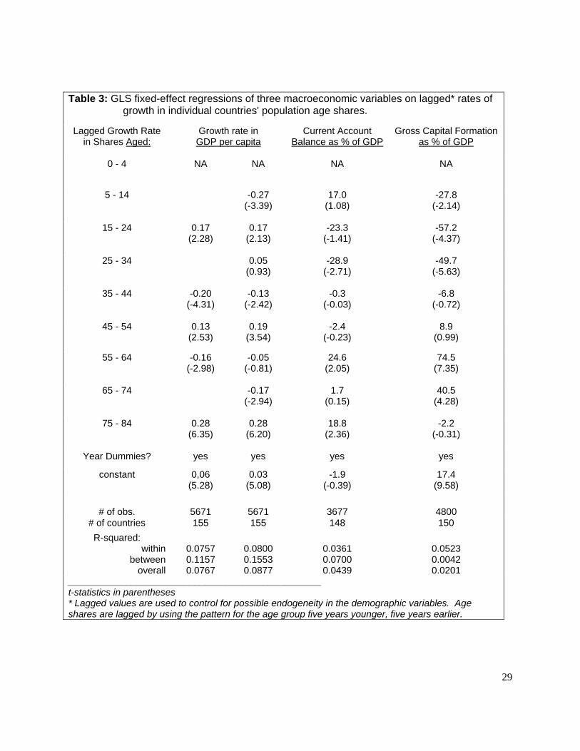
of over-fitting the data. In order to guard against this, the regressions have been estimated in Table 3 for
all countries using a selection of age groups, to test for consistency. Because of multicollinearity it is not
possible to include all 17 five-year age groups in the regressions, but ten-year age groups whose effects in
Figure 3 appear to trace out the general shape of the curves for "all countries" have been included: 15-24,
35-44, 45-54, 55-64, and 75-84. The result of this regression is presented in the first column of results in
Table 3, where it can be seen that there is a direct correspondence between the results of the two
approaches, in terms of the sign of the effects. No doubt without the corroboration of the Fair-
Dominguez method, one might assume that the many changes in sign in the first column of Table 3 were
due to simple multicollinearity, rather than representative of true age group effects on per capita GDP
growth.
In fact, the use of a complete set of lagged ten-year age groups produces the same pattern of effect as that
shown in Figure 3, as illustrated in the second column of results in Table 3: a positive and significant
effect of the 15-24, 45-54 and 75-84 age groups, with a significant negative effect of the 35-44 and 64-74
age groups.5 Apparently the correlations among these growth rates, shown in Table 4, are not high
enough, for "all countries", to create spurious signs in a more complete regression.
5 Some comparison can be made here with findings in Feyrer(2007,2008), who imputes a significant positive effect on output of first differences in the share of the work force aged 40-49, with a negative coefficient on the share aged 20-29. There are a few differences in approach here, in that this study uses rates of change, rather than first difference, in population shares and uses slightly different age groupings (45-54 and 15-24). In addition, Feyrer looks only at the workforce aged 10-69, rather than the full population and age groups, as in this paper. However,

18
The 15-24 age group, which has such a consistently positive effect on per capita GDP growth, has
consistently negative effects on a countries' current account balance (CAB) and gross capital formation
(GCF). This is shown in the third and fourth columns of results in Table 3, where the effect of the 15-24
age group is negative at about the 0.15 level of significance for the CAB, while the effect is negative and
significant at higher than a 0.001 level for GCF. Their strong positive effect on consumption would tend
to increase imports, thus reducing the CAB, and drain funds away from capital formation in favor of
current consumption, thus reducing GCF.
In addition to the effect of changes in a country’s own age distribution, there could be strong effects of
changes that occur in that country’s trading partners’ age distributions. For example, if growth of the
share of 15-24 year olds in the U.S. increases the U.S.’s tendency to import goods, that would have a
direct effect on U.S. trading partners, where exports would increase. Thus one would expect an
improvement in the current account balance (CAB) of less developed countries with whom the U.S.
trades. Similarly, if gross capital formation (GCF) in the U.S. is negatively affected by increases in the
proportion there aged 15-24, then FDI from the U.S. to other countries might also be reduced.
However if, after a period of strong increases, the share of the U.S. population aged 15-24 were to
decline, the U.S. economy would slow and U.S. trading partners would feel negative repercussions:
“Crashes are more likely if growth in industrial countries has been sluggish. A possible channel is through lower demand for developing country exports, a decline in foreign exchange reserves, and a more likely collapse of the currency.” (Milesi-Ferretti & Razin, 2000:308)
the results in Table 3 and in Figure 3 also show a significant positive effect of the 45-54 group. Direct comparisons for the 15-24 group can't be made, however, since Feyrer's negative coefficient on the 20-29 age group simply indicates that the coefficient on the 20-29 age group is less than that on the 40-49 group. This is supported by the finding in column 2 of Table 3, although the difference is slight.

19
That hypothesis, of effects on trading partners, has been tested by regressing the CAB, GCF, and GDP –
in the Asian Tigers and the Tequila group, and in OECD and non-OECD countries – on changes in the
proportion aged 15-24 in the U.S. The results of those regressions are presented in Table 5, where it can
be seen that there are indeed significant effects. They in general support the hypothesis outlined above.
The effect on GDP in all groups except the Asian Tigers is positive and highly significant. The effect on
CAB is positive for all groups, and significant in all cases except for the Tequila Group. The effect on
GCF is more mixed, with highly significant effects in all groups, but negative only in "all countries", the
Asian Tigers, and non-OECD countries.
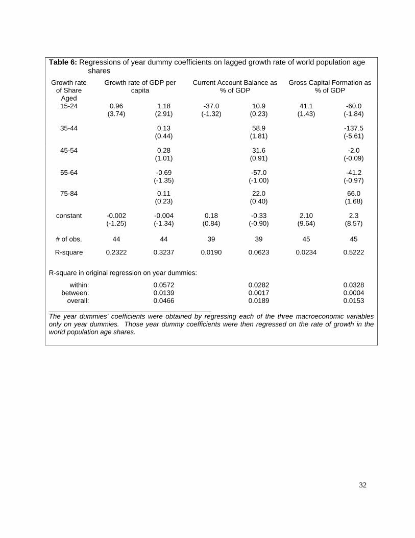
Another way of looking at the strength of the effect of the 15-24 age group can be seen in Table 6, where
the three macroeconomic variables – GDP, CAB, and GCF – have been regressed just on a set of year
dummies, in order to ascertain the overall time pattern of each variable at the global level over the 45 year
period. The coefficients of these regressions have then been regressed on the world's lagged population
age share growth rates, using the age groups indicated by the pattern for "all countries" in Figure 3. The
results are not impressive for CAB and GCF, suggesting that the population variables do not have a very
significant effect overall. This is understandable when one considers the differential effect of own versus
trading partner age patterns. In addition, the actual explanatory power of the original regression used to
obtain the coefficients was quite low, explaining less than 0.02 of variation overall. But the effect is much
more significant for GDP (with an overall R-square in the original regression of 0.0466), where the effect
of the 15-24 age group is overwhelmingly positive both in terms of a country's own population as well as
in terms of the population of trading partners. There we see a surprisingly high proportion of the global
time pattern of change in GDP being explained by demographic variables. The R-square for the full
regression in the second column is a high 0.3237, with the 15-24 age group carrying most of the
explanatory power. The R-square for the 15-24 age group on its own is 0.2322.
20
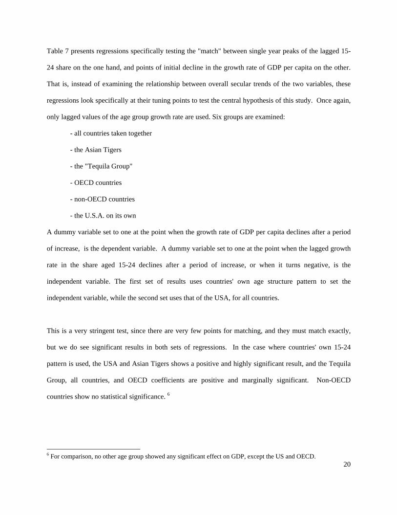
Table 7 presents regressions specifically testing the "match" between single year peaks of the lagged 15-
24 share on the one hand, and points of initial decline in the growth rate of GDP per capita on the other.
That is, instead of examining the relationship between overall secular trends of the two variables, these
regressions look specifically at their tuning points to test the central hypothesis of this study. Once again,
only lagged values of the age group growth rate are used. Six groups are examined:
- all countries taken together
- the Asian Tigers
- the "Tequila Group"
- OECD countries
- non-OECD countries
- the U.S.A. on its own
A dummy variable set to one at the point when the growth rate of GDP per capita declines after a period
of increase, is the dependent variable. A dummy variable set to one at the point when the lagged growth
rate in the share aged 15-24 declines after a period of increase, or when it turns negative, is the
independent variable. The first set of results uses countries' own age structure pattern to set the
independent variable, while the second set uses that of the USA, for all countries.
This is a very stringent test, since there are very few points for matching, and they must match exactly,
but we do see significant results in both sets of regressions. In the case where countries' own 15-24
pattern is used, the USA and Asian Tigers shows a positive and highly significant result, and the Tequila
Group, all countries, and OECD coefficients are positive and marginally significant. Non-OECD
countries show no statistical significance. 6
6 For comparison, no other age group showed any significant effect on GDP, except the US and OECD.
21
The second set of results in Table 7, using a dummy for the USA's 15-24 pattern as the independent
variable in all cases, shows a strong dependence of other countries on changes in the U.S. share aged 15-
24. All except the Tequila Group show a significant result. The Asian Tigers are significant only at the
0.10 level, but for the OECD, all countries taken together, non-OECD countries and of course the U.S.,
the result is positive and highly significant.7
Table 8 presents the number and percentage of times, for each group of countries, in which there is a
coincidence between an initial decline in the growth rates of both GDP per capita and the (lagged) share
aged 15-24. The upper half of the table considers coincidences with the USA pattern of changes in the
15-24 group, while the bottom half looks at coincidences using the countries' own pattern of changes in
the 15-24 group. This table shows that in nearly all cases, more than 70% of the times when the growth
rate of the share aged 15-24, declined, the growth rate of GDP per capita also declined, in the same or
adjacent period. For the USA this occurred 100% of the time.
Table 9 presents the same type of information as Table 8, except that here the focus is not on simple
declines in the growth rate, but rather periods in which the growth rate actually turns negative – that is,
when GDP per capita declines on an absolute basis. There we can see that for countries overall, there was
a coincidence between the decline in GDP and the U.S. change in the 15-24 group 45.6 percent of the
time; and for countries' own change in the 15-24 group, this occurred 50.1 percent of the time.
V. Patterns of Change in Age Shares
Figures 4-7 examine graphically the approach used in Tables 7, 8 and 9. That is, they look at the actual
time pattern of (lagged) growth rates in the 15-24 share, to show instances where financial crises
correspond with turning points in the demographic variable. 15-24 is a very broad age group, and it is
7 Again, for comparison, in this case no other age group showed any significant effect, for any country group.
22
likely that the effects studied here will occur at various points within that age group, depending on the
level of educational attainment in a country. For this reason, the graphs in Figures 4-7 make use of two
subsets of the 15-24 age group: 15-19 in less developed countries, and 20-24 in the industrialized nations.
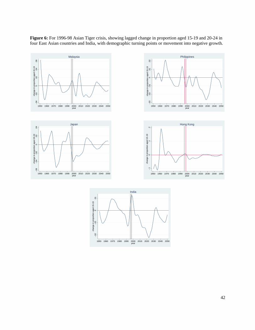
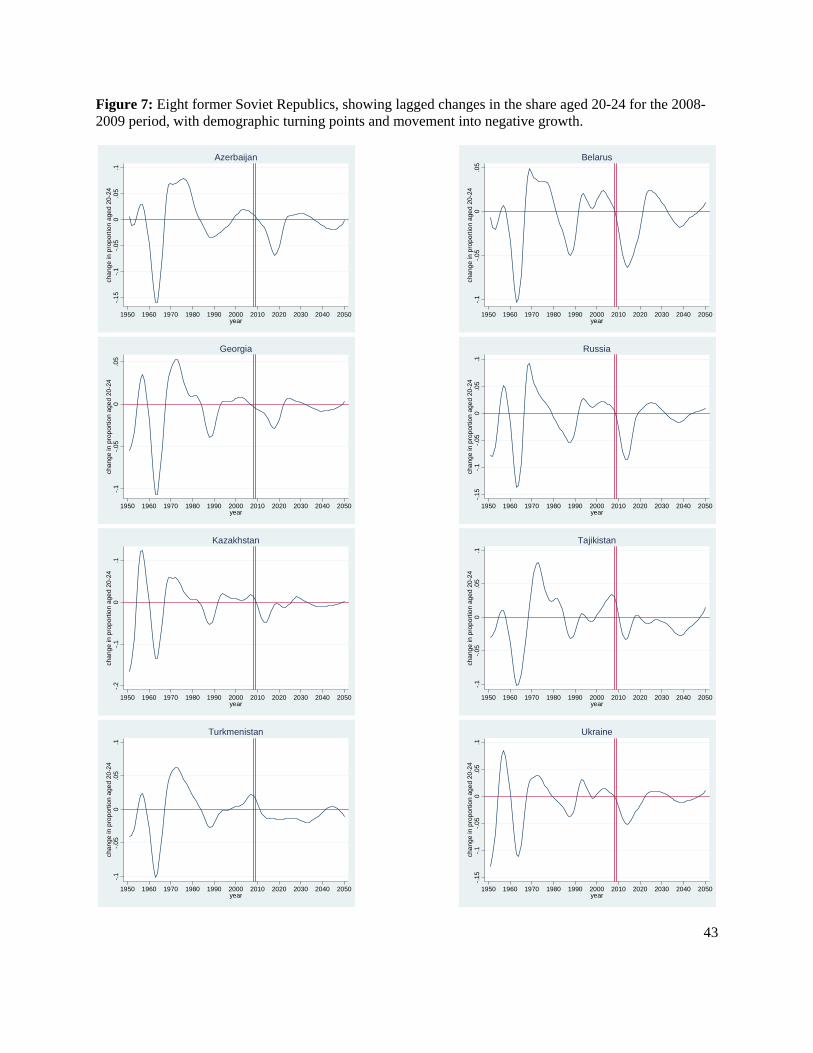
Figures 4-7 present graphs for the 1980-82, 1992-94 ("Tequila" crisis), 1996-98 (Asian Tigers' crisis), and
2008-2009 periods, respectively, where in country after country one sees a dip into declining 15-24
growth rates during each crisis period, or even movements into negative growth rates.
Figure 4 presents graphs for five Latin American countries (Brazil, Chile, Colombia, Peru, Uruguay and
Venezuela) and nine industrialized nations (Austria, Canada, Germany, Great Britain, Italy, Netherlands,
Russia, Spain and the U.S.) that all experienced either the beginning of a downturn in growth rates, or
even a movement into negative growth rates in the 1980-1982 period of economic turmoil.
Figure 5 presents a similar picture for seven countries (Argentina, Brazil, Colombia, Ecuador, Peru,
Uruguay and Venezuela) involved in the crisis among what has become to be known as the Tequila
Group, in 1992-1994. Figure 6 in turn presents graphs for two of the Asian Tigers affected in the 1996-
1998 crisis (Malaysia and the Philippines), together with three countries closely associated with them
(Japan, Hong Kong and India), all of which experienced similar downturns, or movements into negative
growth, in the key age groups. Here, as many have pointed out, there appears to have been a "contagion
effect" in the development of the crisis.
And finally, Figure 7 presents some of the extremely large number of countries that have or are
experiencing downturns or movements into negative 15-24 growth in this 2008-2009 crisis period: eight
former Soviet Republics – Russia, Belarus, Georgia, Ukraine, Azerbaijan, Kazakhstan, Tajikistan and
Turkmenistan; seven industrialized nations – Belgium, Germany, Great Britain, Netherlands, Norway,
Sweden and the U.S.; and six Latin American countries – Bolivia, Colombia, El Salvador, Honduras,

23
Nicaragua and Puerto Rico. The OECD countries, which had averaged in the decade before the 2008-
2009 crisis, only 1.8 declines per year in the growth rate of the 15-24 group, experienced seven in 2008
and nine in 2009.
All of the graphs in Figures 4-7 are summarized in Table 10: an impressive array of occurrences in which
economic actors must have experienced a fairly sharp jolt to their expectations of continually increasing
rates of growth.
VI. Conclusions
At least two things appear clear from the previous analyses. One is that there are significant effects of
changing demographics on economic indicators: growth in GDP especially, as many have suggested
earlier, but also the current account balance (CAB), and gross capital formation (GCF). The 15-24 age
group appears to be key in these effects, with increases in that age group exerting strong positive effects
on GDP growth, and negative effects on the CAB and GCF. The second is that there have been major
shifts in demographic age structure – especially the share of the population aged 15-24 – during the past
half century or more, many of which correspond closely to periods of institutional turmoil. The
hypothesis presented in this paper, which appears to be supported by the data, is that increases in the share
of the 15-24 age group lead producers to ratchet up their production expectations and take out loans to
expand production capacity; but then reductions in that share – or even declining rates of increase –
confound these expectations and precipitate a downward spiral of missed loan payments and even defaults
and bankruptcies, putting pressure on central banks and causing foreign investors to withdraw funds and
speculators to unload the local currency.
This appears to have been the pattern not only during the 1996-98 crisis with the Asian Tigers, but also
during the “Tequila” crisis of the early 1990s, the crises that occurred in the early 1980s, among

24
developed as well as developing nations, and the economic downturn experienced by Japan after about
1990. The effect is even more pronounced for the current 2008-2009 period. These results suggest that a
good deal more study of demographic effects is warranted.

25
Bibliography Bloom, D.E and J.G.Williamson (1998). “Demographic Transitions and Economic Miracles in Emerging
Asia”. World Bank Economic Review, 12(3):419-455. Bloom, D.E. and J.E.Finlay (2009). "Demographic Change and Economic Growth in Asia", Asian
Economic Policy Review, (2009)4:45-64. Calvo, Guillermo (2000). “Balance-of-Payments Crises in Emerging Markets”, pp.71-104 in Allan
Krugman (ed.) Currency Crises. University of Chicago Press. Della Vigna, S. and J.M.Pollet (2007). "Demographics and Industry Returns" American Economic
Review, December, 97(5):1667-1702. Easterlin, R.A. (1996) Growth Triumphant: The Twenty-First Century in Historical Perspective. Ann
Arbor: University of Michigan Press. Fair, Ray C. and Kathryn Dominguez (1991). “Effects of the changing U.S. age distribution on
macroeconomic equations”, American Economic Review, 81(5):1276-1294. Feyrer, James (2007) "Demographics and Productivity" Review of Economics and Statistics, 89(1):100-
109. Feyrer, James (2008) "Aggregate Evidence on the Link Between Demographics and Productivity"
Population and Development Review, March 2008 , 34(supplement):78-99. Frankel, J.A. (2000). Panel Presentation: Involving the Private Sector in Crisis Resolution”, pp.327-338 in
Alan Krugman (ed.) Currency Crises. University of Chicago Press. Galbraith, J.K. (1958). “The Dependence Effect” in The Affluent Society. Boston: Houghton-Mifflin. Higgins, Matthew (1998). “Demography, National Savings, and International Capital Flows” International Economic Review, 39(2):343-369. Higgins M and Williamson JG (1997). “Age Structure Dynamics in Asia and Dependence on Foreign
Capital” Population and Development Review, 23(2):262-293. Judge, George G., W.E.Griffiths, R.Carter-Hill, H. Lütkepohl and Tsoung-Chao Lee (1985). The Theory
and Practice of Econometrics, Second Edition, John Wiley and Sons: New York. Keynes, J.M. (1937). “Some Economic Consequences of a Declining Population.” Eugenics Review,
29(1):13-17. Krugman, Alan (2000). “Introoduction”, Currency Crises. University of Chicago Press. Macunovich, D.J. (2007). “Effects of Changing Age Structure and Intergenerational Transfers on Patterns
of Consumption and Saving”, pages 243 - 277 in Allocating Public And Private Resources Across Generations, edited by Anne Gauthier, Cyrus Chu and Shripad Tuljapurkar. Springer/Kluwer Academic Publishers: Dordrecht, The Netherlands.
26
Milesi-Feretti, G.M. and A. Razin (2000). Current Account Reversals and Currency Crises: Empirical Regularities, pp.285-326 in Alan Krugman (ed.) Currency Crises. University of Chicago Press.
Pesenti, P. and C. Tille (2000). “The Economics of Currency Crises and Contagion: An Introduction”,
FRBNY Economic Policy Review, September, p.3-16. Rostow, W.W. (1998). The Great Population Spike and After: Reflections on the 21st Century. Oxford
University Press. Schumpeter, J.A. (1946) “The American Economy in the Interwar Period: The Decade of the Twenties”,
American Economic Review 36:1-10. United Nations (1999). World Population 1950-2050 (the 1998 Revision). Diskette, United Nations, New
York. Unites States Bureau of the Census (1996). Diskette, U.S. population by single year of age, 1900-1995
and projections to 2050, July 1, 1996. World Bank Group (2007). World Development Indicators (WDI). online at http://ddp-ext.worldbank.org/ext/DDPQQ/member.do?method=getMembers&userid=1&queryId=135

27
Table 1: Summary statistics for key variables
Rate of growth of share of population
aged 15-24
Rate of change in GDP per capita
Current Account Balance as
percent of GDP
Gross Capital Formation as
percent of GDP
range -.204, .301 -.505, .898 -48.1, 56.7 0, 113.5
mean .0007 .020 -3.03 22.47
Standard deviation .017 .065 8.49 10.32
Percentiles: 10%
-.018
-.042
-11.79
11.92
25% -.007 -.004 -6.46 16.33
50% .001 .022 -2.71 21.00
75% .009 .046 0.55 26.63
90% .019 .076 4.91 33.97
Number of single-year observations
with values in excess of three
std.dev.from mean
132 below 82 above
54 below 52 above
49 below 38 above
0 below (0) 95 above
28
Table 2: GLS fixed-effects regressions of growth in per capita GDP on lagged* vectors of
changes in population age shares. All Countries Asian Tigers Tequila Group USA and Japan # of obs 5671 225 224 90 # of countries 155 5 5 2 R-sq: within 0.0758 0.6136 0.3702 0.5067 between 0.0109 0.3942 0.2545 1.0000 overall 0.0694 0.4804 0.3676 0.0197 z1 -0.0257 -0.0054 0.0088 -0.1788 (-2.25) (-0.26) (1.38) (-3.10) z2 0.0051 0.0017 -0.0002 0.0266 (3.50) (0.77) (-1.46) (3.33) z3 -0.0004 -0.0001 1.91e-06 -0.0017 (-4.35) (-1.06) (1.44) (-3.38) z4 1.31e-05 2.85e-06 5.36e-05 (4.96) (1.24) (3.38) z5 -2.38e-07 -3.36e-08 -9.17e-07 (-5.43) (-1.37) (-3.34) z6 2.16e-09 1.47e-10 7.95e-09 (5.79) (1.45) (3.27) z7 -7.76E-12 -2.74e-11 (-6.07) (-3.20) Year
Dummies?
yes
yes
yes
no** constant 0.025 0.049 0.030 0.249 (4.25) (3.11) (1.39) (1.65) __________________________________________ t-statistics in parentheses * Lagged values are used to control for possible endogeneity in the demographic variables. Age shares are lagged by using the pattern for the age group five years younger, five years earlier. ** The 45 year dummies were omitted from the last regression because of the small number of observations.
29
Table 3: GLS fixed-effect regressions of three macroeconomic variables on lagged* rates of
growth in individual countries' population age shares.
Lagged Growth Rate in Shares Aged:
Growth rate in GDP per capita
Current Account Balance as % of GDP
Gross Capital Formation as % of GDP
0 - 4 NA NA NA NA
5 - 14 -0.27 (-3.39)
17.0 (1.08)
-27.8 (-2.14)
15 - 24 0.17 (2.28)
0.17 (2.13)
-23.3 (-1.41)
-57.2 (-4.37)
25 - 34 0.05 (0.93)
-28.9 (-2.71)
-49.7 (-5.63)
35 - 44 -0.20 (-4.31)
-0.13 (-2.42)
-0.3 (-0.03)
-6.8 (-0.72)
45 - 54 0.13 (2.53)
0.19 (3.54)
-2.4 (-0.23)
8.9 (0.99)
55 - 64 -0.16 (-2.98)
-0.05 (-0.81)
24.6 (2.05)
74.5 (7.35)
65 - 74 -0.17 (-2.94)
1.7 (0.15)
40.5 (4.28)
75 - 84 0.28 (6.35)
0.28 (6.20)
18.8 (2.36)
-2.2 (-0.31)
Year Dummies? yes yes yes yes
constant 0,06 (5.28)
0.03 (5.08)
-1.9 (-0.39)
17.4 (9.58)
# of obs.
5671
5671
3677
4800
# of countries 155 155 148 150 R-squared:
within between
overall
0.0757 0.1157 0.0767
0.0800 0.1553 0.0877
0.0361 0.0700 0.0439
0.0523 0.0042 0.0201
________________________________________________ t-statistics in parentheses * Lagged values are used to control for possible endogeneity in the demographic variables. Age shares are lagged by using the pattern for the age group five years younger, five years earlier.

30
Table 4: Correlations among growth rates in population age shares 0 - 4 5 - 14 15 - 24 25 - 34 35 - 44 45 - 54 55 - 64 65 - 74 75 - 84 0 – 4 1.0000 5 – 14 0.7015 1.0000 15 – 24 0.3425 0.3741 1.0000 25 – 34 0.0592 -0.0751 0.1008 1.0000 35 – 44 -0.4897 -0.3218 -0.2003 0.0690 1.0000 45 – 54 -0.5925 -0.6512 -0.2767 -0.0008 0.3499 1.0000 55 – 64 -0.5833 -0.6215 -0.5523 -0.0829 0.3268 0.6179 1.0000 65 – 74 -0.5959 -0.6272 -0.4919 -0.2229 0.3177 0.6068 0.7921 1.0000 75 - 84 -0.5413 -0.5787 -0.4783 -0.1648 0.2365 0.5717 0.7589 0.8729 1.0000

31
Table 5: GLS fixed-effects estimates of effect on other countries, of growth rate in USA share aged 15-24
All
Countries Asian Tigers
Tequila Group
OECD Countries
Non-OECD Countries
Current Account Balance # of obs 3919 143 154 888 3031 # of groups 170 5 5 29 141 R-square: within 0.0033 0.2103 0.0048 0.0086 0.0034 between 0.0206 0.0254 0.0732 0.0773 0.0154 overall 0.0050 0.2040 0.0064 0.0068 0.0043 est. coeff. on Δ in U.S.share 15-24 37.7 200.8 16.3 21.7 43.4 t-statistic (3.54) (6.04) (0.84) (2.72) (3.12) Gross Capital Formation # of obs 5042 228 229 1031 4011 # of groups 171 5 5 28 143 R-square: within 0.0007 0.3528 0.1058 0.0303 0.0035 between 0.0274 0.0924 0.0493 0.0178 0.0339 overall 0.0016 0.2990 0.0934 0.0211 0.0047 est. coeff. on Δ in U.S.share 15-24 -12.6 -254.5 66.9 56.1 -29.3 t-statistic (-1.89) (-11.00) (5.14) (5.60) (-3.69) Growth in per capita GDP # of obs 5995 228 224 1221 4774 # of groups 179 5 5 29 150 R-square: within 0.0262 0.0155 0.0548 0.0692 0.0246 between 0.0581 0.0244 0.3116 0.0603 0.0583 overall 0.0206 0.0133 0.0538 0.0658 0.0182 est. coeff. on Δ in U.S.share 15-24 0.58 -0.24 0.54 0.43 0.62 t-statistic (12.52) (-1.86) (3.55) (9.41) (10.80)
32
Table 6: Regressions of year dummy coefficients on lagged growth rate of world population age
shares Growth rate
of Share Aged
Growth rate of GDP per capita
Current Account Balance as % of GDP
Gross Capital Formation as % of GDP
15-24 0.96 (3.74)
1.18 (2.91)
-37.0 (-1.32)
10.9 (0.23)
41.1 (1.43)
-60.0 (-1.84)
35-44 0.13 (0.44)
58.9 (1.81)
-137.5 (-5.61)
45-54 0.28 (1.01)
31.6 (0.91)
-2.0 (-0.09)
55-64 -0.69 (-1.35)
-57.0 (-1.00)
-41.2 (-0.97)
75-84 0.11 (0.23)
22.0 (0.40)
66.0 (1.68)
constant -0.002 (-1.25)
-0.004 (-1.34)
0.18 (0.84)
-0.33 (-0.90)
2.10 (9.64)
2.3 (8.57)
# of obs. 44 44 39 39 45 45
R-square 0.2322 0.3237 0.0190 0.0623 0.0234 0.5222
R-square in original regression on year dummies:
within: between:
overall:
0.0572 0.0139 0.0466
0.0282 0.0017 0.0189
0.0328 0.0004 0.0153
___________________________________________ The year dummies' coefficients were obtained by regressing each of the three macroeconomic variables only on year dummies. Those year dummy coefficients were then regressed on the rate of growth in the world population age shares.

33
Table 7: GLS fixed-effect regressions1 to test whether initial declines in the lagged growth rate in
share 15-24 match initial downturns in growth rate of GDP per capita.
All Countries
Asian Tigers
Tequila Group
OECD
Non-OECD Countries
USA1
Using each country's own lagged growth rate in share aged 15-24:
Initial decline or turn to negative in lagged growth rate of 15-24?
0.0188 (1.31)*
0.191
(1.91)***
0.159 (1.48)*
0.067
(1.67)**
0.010 (0.62)
1.34
(2.45)***
constant 0.19 (44.19)
0.25 (8.11)
0.26 (8.68)
0.25 (19.78)
0.18 (39.61)
-0.77 (-3.54)
R-square: within:
between: overall:
0.0002 0.0112 0.0001
0.0153 0.0336 0.0154
0.0092 0.0021 0.0092
0.0020 0.0259 0.0022
0.0001 0.0070 0.0000
0.1107
Using USA's lagged growth rate in share aged 15-24:
Initial decline or turn to negative in lagged USA growth rate of 15-24?
0.054
(4.73****
0.137
(1.72)**
-0.021 (-0.25)
0.161
(4.98)****
0.026
(2.83)****
1.34
(2.45)***
constant 0.18 (41.47)
0.23 (7.66)
0.28 (8.82)
0.22 (17.76)
0.18 (37.51)
-0.77 (-3.54)
R-square: within:
between: overall:
0.0026 0.0002 0.0024
0.0124
. 0.0124
0.0003
. 0.0003
0.0179 0.0000 0.0175
0.0011 0.0003 0.0010
0.1107
_____________________________________________ Dependent variable is a dummy set to one for a year in which the GDPpc growth rate drops after increasing
in previous period t-statistics in parentheses 1Probit was used for the USA regression For the USA over a 45-year period, the independent variable takes on the value of "1" for seven years, and
five of those correspond to a "1" in the dependent variable. The other two are off by just one year (with the change in 15-24 immediately preceding the change in GDP per capita).
* significant at the .25 level ** significant at the .10 level *** significant at the .05 level ****significant at the .005 level

34
Table 8: Number and percent of times when decline in growth rate of GDP per capita
coincided with (lagged) decline in growth rate of 15-24 age group share.
Group
Total number of declines in
GDP per capita
Total number of declines in growth rate of 15-24 group*
Number of matches +1**
Number of matches ± 1***
Percent of matches ± 1****
Based on decline in USA 15-24: All countries 1,688 899 596 726 80.8
OECD 337 189 138 159 84.1
Non-OECD 1,351 710 458 567 79.9
Asian Tigers 61 35 27 29 82.9
Tequila Group 66 35 22 28 80.0
USA 14 7 6 7 100.0
Japan 10 7 4 5 71.4
Mexico 13 7 4 6 85.7
Canada 11 6 5 6 100.0
Great Britain 12 7 4 5 71.4
Germany 10 5 5 5 100.0
Based on decline in countries' own 15-24:
All countries 1,688 557 321 436 78.3
OECD 337 124 77 94 75.8
Non-OECD 1,351 433 244 342 79.0
Asian Tigers 61 21 13 18 85.7
Tequila Group 66 19 10 17 89.5
Japan 10 5 2 2 40.0
Mexico 13 3 2 3 100.0
Canada 11 3 1 2 66.7
Great Britain 12 6 3 5 83.3
Germany 10 3 2 2 66.7
* Number of declines in 15-24 in periods when own GDP per capita was reported. ** Number of times when GDP decline occurred in same year as 15-24 decline, or in following year. *** Number of times when GDP decline occurred in same year as 15-24 decline, or in a year just before or
after. **** This is the percent of total declines in the growth rate of the 15-24 group that coincided with a decline in
the growth rate of GDP per capita.

35
Table 9: Number and percent of times when a decline in GDP per capita (negative growth)
coincided with (lagged) decline in growth rate of 15-24 age group share.
Group
Total number of negative GDP per
capita
Total number of declines in growth rate of 15-24 group*
Number of matches +1**
Number of matches ± 1***
Percent of matches ± 1****
Based on decline in USA 15-24: All countries 1,664 899 313 410 45.6
OECD 167 189 27 46 24.3
Non-OECD 1,497 710 286 364 51.3
Asian Tigers 25 35 5 8 22.9
Tequila Group 59 35 11 15 42.9
USA 7 7 2 3 42.9
Japan 5 7 2 2 28.6
Mexico 8 7 2 2 25.0
Canada 5 6 0 1 16.7
Great Britain 6 7 1 1 14.3
Germany 6 5 1 2 40.0
Based on decline in countries' own 15-24:
All countries 1,664 557 216 279 50.1
OECD 167 124 24 32 25.8
Non-OECD 1,497 433 192 247 57.0
Asian Tigers 25 21 3 5 23.8
Tequila Group 59 19 7 9 47.4
Japan 5 5 0 0 0.0
Mexico 8 3 1 1 33.3
Canada 5 3 0 0 0.0
Great Britain 6 6 1 1 16.7
Germany 6 3 1 1 33.3
* Number of declines in 15-24 in periods when own GDP per capita was reported. ** Number of times when negative GDP occurred in same year as 15-24 decline, or in following year. *** Number of times when negative GDP occurred in same year as 15-24 decline, or in a year just before or after. **** This is the percent of total declines in the growth rate of the 15-24 group that coincided with an absolute decline
in GDP per capita.

36
Table 10: Some of the countries that experienced downturns in the periods indicated, in growth
rates of age groups indicated 1980 - 1982 1992 - 1994 1996 - 1998 2008-2009
15 - 19: Brazil* Argentina Hong Kong Bolivia* Chile* Brazil India Colombia Colombia* Colombia Malaysia El Salvador Peru* Ecuador* Philippines* Honduras* Venezuela* Peru Nicaragua Uruguay* Puerto Rico Venezuela
20 - 24: Austria Japan* Belgium Canada* Germany* Germany Great Britain Great Britain Netherlands Italy* Norway Netherlands Sweden Russia* USA Spain Belarus* USA* Georgia* Russia* Kazakhstan Tajikistan Turkmenistan Uzbekhistan Ukraine* * asterisk indicates an age group whose growth rate not only declined -- it actually turned negative in or very
near the period indicated

37
Figure 1: The curve on the graph represents a three year moving average of the (one year) lagged annual rate of change in the proportion of young adults in the U.S. population, as reported by the U.S. Census Bureau. “Young adults” are defined as those aged 15-19 prior to 1950, and 20-24 in the years after, given changing levels of education over time. The vertical lines mark the start of recessions, as defined by NBER. There is a very close correspondence between the vertical lines, and peaks in the curve, as well as points where the curve goes negative. In addition, the deep trough between 1937 and 1958 contained another four recessions, and there were two in the trough between 1910 and 1920 (not marked on the graph). The only recessions over the last one hundred years that don’t appear to correspond to features of the curve, are those in 1920, 1926 and 1960. Figure 2: The curve on this graph indicates annual rates of change in the (five year) lagged proportion aged 15-24 in Japan's population. The vertical lines indicate the period that has generally been referred to as Japan's "lost decade".
-.04
-.02
0.0
2.0
4C
hang
e in
Pop
ulat
ion
Sha
re
1900 1910 1920 1930 1940 1950 1960 1970 1980 1990 2000 2010 2020 2030 2040 2050Year
Change in Population Share of Young Adults in the U.S.
-.06
-.04
-.02
0.0
2ch
ange
in p
ropo
rtion
age
d 20
-24
1950 1960 1970 1980 1990 2000 2010 2020 2030 2040 2050year
Change in Population Share of Young Adults in Japan

38
Figure 3: Estimated coefficients on age groups, in terms of effect on growth rate of GDP per capita. Vertical bars demarcate the 15-24 age group. Lagged values of age groups' growth rates are used, to control for possible endogeneity of demographic variables.
-.06
-.04
-.02
0.0
2.0
4co
effic
ient
on
age
shar
e
0 20 40 60 80age
Asian Tigers
-.04
-.02
0.0
2.0
4co
effic
ient
on
age
shar
e
0 20 40 60 80age
All countries
-.04
-.02
0.0
2.0
4co
effic
ient
on
age
shar
e
0 20 40 60 80age
Tequila Group-.2
-.10
.1.2
coef
ficie
nt o
n ag
e sh
are
0 20 40 60 80age
USA and Japan

39
Figure 4: For 1980-82, lagged change in proportion aged 15-19 in five Latin American countries and in proportion aged 20-24 in three industrialized countries, showing demographic turning points or movement into negative growth.
-.02
-.01
0.0
1.0
2.0
3ch
ange
in p
ropo
rtion
age
d 15
-19
1950 1960 1970 1980 1990 2000 2010 2020 2030 2040 2050year
Brazil
-.03
-.02
-.01
0.0
1.0
2ch
ange
in p
ropo
rtion
age
d 15
-19
1950 1960 1970 1980 1990 2000 2010 2020 2030 2040 2050year
Chile
-.015
-.01
-.005
0.0
05.0
1ch
ange
in p
ropo
rtion
age
d 15
-19
1950 1960 1970 1980 1990 2000 2010 2020 2030 2040 2050year
Peru
-.06
-.04
-.02
0.0
2.0
4C
hang
e in
20-
24 a
ge s
hare
1950 1960 1970 1980 1990 2000 2010 2020 2030 2040 2050year
Austria
-.05
0.0
5C
hang
e in
20-
24 a
ge s
hare
1950 1960 1970 1980 1990 2000 2010 2020 2030 2040 2050year
Canada
-.1-.0
50
.05
Cha
nge
in 2
0-24
age
sha
re
1950 1960 1970 1980 1990 2000 2010 2020 2030 2040 2050year
Germany
-.02
-.01
0.0
1.0
2ch
ange
in p
ropo
rtion
age
d 15
-19
1950 1960 1970 1980 1990 2000 2010 2020 2030 2040 2050year
Venezuela
-.03
-.02
-.01
0.0
1.0
2ch
ange
in p
ropo
rtion
age
d 15
-19
1950 1960 1970 1980 1990 2000 2010 2020 2030 2040 2050year
Colombia

40
Figure 4 cont’d: For 1980-82, lagged change in proportion aged 20-24 in six industrialized nations, showing demographic turning points or movement into negative growth.
-.04
-.02
0.0
2.0
4C
hang
e in
20-
24 a
ge s
hare
1950 1960 1970 1980 1990 2000 2010 2020 2030 2040 2050year
Great Britain
-.06
-.04
-.02
0.0
2C
hang
e in
20-
24 a
ge s
hare
1950 1960 1970 1980 1990 2000 2010 2020 2030 2040 2050year
Spain
-.04
-.02
0.0
2.0
4C
hang
e in
20-
24 a
ge s
hare
1950 1960 1970 1980 1990 2000 2010 2020 2030 2040 2050year
United States
-.15
-.1-.0
50
.05
.1ch
ange
in p
ropo
rtion
age
d 20
-24
1950 1960 1970 1980 1990 2000 2010 2020 2030 2040 2050year
Russia
-.04
-.02
0.0
2.0
4.0
6C
hang
e in
20-
24 a
ge s
hare
1950 1960 1970 1980 1990 2000 2010 2020 2030 2040 2050year
Netherlands
-.06
-.04
-.02
0.0
2ch
ange
in p
ropo
rtion
age
d 20
-24
1950 1960 1970 1980 1990 2000 2010 2020 2030 2040 2050year
Italy

41
Figure 5: For 1992-1994 Tequila Crisis, showing lagged change in proportion aged 15-19 in seven Latin American countries, with demographic turning points or movement into negative growth.
-.02
-.01
0.0
1.0
2.0
3ch
ange
in p
ropo
rtion
age
d 15
-19
1950 1960 1970 1980 1990 2000 2010 2020 2030 2040 2050year
Argentina
-.02
-.01
0.0
1.0
2.0
3ch
ange
in p
ropo
rtion
age
d 15
-19
1950 1960 1970 1980 1990 2000 2010 2020 2030 2040 2050year
Brazil
-.01
0.0
1.0
2.0
3ch
ange
in p
ropo
rtion
age
d 15
-19
1950 1960 1970 1980 1990 2000 2010 2020 2030 2040 2050year
Ecuador
-.015
-.01
-.005
0.0
05.0
1ch
ange
in p
ropo
rtion
age
d 15
-19
1950 1960 1970 1980 1990 2000 2010 2020 2030 2040 2050year
Peru
-.03
-.02
-.01
0.0
1.0
2ch
ange
in p
ropo
rtion
age
d 15
-19
1950 1960 1970 1980 1990 2000 2010 2020 2030 2040 2050year
Uruguay
-.03
-.02
-.01
0.0
1.0
2ch
ange
in p
ropo
rtion
age
d 15
-19
1950 1960 1970 1980 1990 2000 2010 2020 2030 2040 2050year
Colombia
-.02
-.01
0.0
1.0
2ch
ange
in p
ropo
rtion
age
d 15
-19
1950 1960 1970 1980 1990 2000 2010 2020 2030 2040 2050year
Venezuela
42
Figure 6: For 1996-98 Asian Tiger crisis, showing lagged change in proportion aged 15-19 and 20-24 in four East Asian countries and India, with demographic turning points or movement into negative growth.
-.04
-.02
0.0
2.0
4.0
6ch
ange
in p
ropo
rtion
age
d 15
-19
1950 1960 1970 1980 1990 2000 2010 2020 2030 2040 2050year
Malaysia
-.03
-.02
-.01
0.0
1.0
2ch
ange
in p
ropo
rtion
age
d 15
-19
1950 1960 1970 1980 1990 2000 2010 2020 2030 2040 2050year
Philippines
-.06
-.04
-.02
0.0
2.0
4ch
ange
in p
ropo
rtion
age
d 20
-24
1950 1960 1970 1980 1990 2000 2010 2020 2030 2040 2050year
Japan
-.10
.1.2
chan
ge in
pro
porti
on a
ged
15-1
9
1950 1960 1970 1980 1990 2000 2010 2020 2030 2040 2050year
Hong Kong
-.02
-.01
0.0
1ch
ange
in p
ropo
rtion
age
d 15
-19
1950 1960 1970 1980 1990 2000 2010 2020 2030 2040 2050year
India
43
Figure 7: Eight former Soviet Republics, showing lagged changes in the share aged 20-24 for the 2008-2009 period, with demographic turning points and movement into negative growth.
-.15
-.1-.0
50
.05
.1ch
ange
in p
ropo
rtion
age
d 20
-24
1950 1960 1970 1980 1990 2000 2010 2020 2030 2040 2050year
Azerbaijan
-.1-.0
50
.05
chan
ge in
pro
porti
on a
ged
20-2
4
1950 1960 1970 1980 1990 2000 2010 2020 2030 2040 2050year
Belarus
-.1-.0
50
.05
chan
ge in
pro
porti
on a
ged
20-2
4
1950 1960 1970 1980 1990 2000 2010 2020 2030 2040 2050year
Georgia
-.15
-.1-.0
50
.05
.1ch
ange
in p
ropo
rtion
age
d 20
-24
1950 1960 1970 1980 1990 2000 2010 2020 2030 2040 2050year
Russia
-.2-.1
0.1
chan
ge in
pro
porti
on a
ged
20-2
4
1950 1960 1970 1980 1990 2000 2010 2020 2030 2040 2050year
Kazakhstan
-.1-.0
50
.05
.1ch
ange
in p
ropo
rtion
age
d 20
-24
1950 1960 1970 1980 1990 2000 2010 2020 2030 2040 2050year
Tajikistan
-.1-.0
50
.05
.1ch
ange
in p
ropo
rtion
age
d 20
-24
1950 1960 1970 1980 1990 2000 2010 2020 2030 2040 2050year
Turkmenistan
-.15
-.1-.0
50
.05
.1ch
ange
in p
ropo
rtion
age
d 20
-24
1950 1960 1970 1980 1990 2000 2010 2020 2030 2040 2050year
Ukraine

44
Figure 7 (cont'd): For 2008-2009 crisis, showing lagged change in proportion aged 20-24 in seven industrialized countries, with demographic turning points or movement into negative growth.
-.04
-.02
0.0
2.0
4C
hang
e in
Sha
re A
ged
20-2
4
1950 1960 1970 1980 1990 2000 2010 2020 2030 2040 2050Year
United States
-.02
0.0
2.0
4.0
6ch
ange
in p
ropo
rtion
age
d 20
-24
1950 1960 1970 1980 1990 2000 2010 2020 2030 2040 2050year
Belgium
-.06
-.04
-.02
0.0
2.0
4ch
ange
in p
ropo
rtion
age
d 20
-24
1950 1960 1970 1980 1990 2000 2010 2020 2030 2040 2050year
Sweden
-.1-.0
50
.05
chan
ge in
pro
porti
on a
ged
20-2
4
1950 1960 1970 1980 1990 2000 2010 2020 2030 2040 2050year
Germany
-.04
-.02
0.0
2.0
4ch
ange
in p
ropo
rtion
age
d 20
-24
1950 1960 1970 1980 1990 2000 2010 2020 2030 2040 2050year
Great Britain
-.04
-.02
0.0
2.0
4.0
6ch
ange
in p
ropo
rtion
age
d 20
-24
1950 1960 1970 1980 1990 2000 2010 2020 2030 2040 2050year
Netherlands
-.04
-.02
0.0
2.0
4ch
ange
in p
ropo
rtion
age
d 20
-24
1950 1960 1970 1980 1990 2000 2010 2020 2030 2040 2050year
Norway

45
Figure 7 (cont'd): For 2008-2009 crisis, showing lagged change in proportion aged 15-19 in six Latin American economies, with demographic turning points or movement into negative growth.
-.015
-.01
-.005
0.0
05.0
1ch
ange
in p
ropo
rtion
age
d 15
-19
1950 1960 1970 1980 1990 2000 2010 2020 2030 2040 2050year
Bolivia
-.03
-.02
-.01
0.0
1.0
2ch
ange
in p
ropo
rtion
age
d 15
-19
1950 1960 1970 1980 1990 2000 2010 2020 2030 2040 2050year
Colombia
-.04
-.02
0.0
2ch
ange
in p
ropo
rtion
age
d 15
-19
1950 1960 1970 1980 1990 2000 2010 2020 2030 2040 2050year
El Salvador
-.02
-.01
0.0
1.0
2ch
ange
in p
ropo
rtion
age
d 15
-19
1950 1960 1970 1980 1990 2000 2010 2020 2030 2040 2050year
Honduras
-.03
-.02
-.01
0.0
1.0
2ch
ange
in p
ropo
rtion
age
d 15
-19
1950 1960 1970 1980 1990 2000 2010 2020 2030 2040 2050year
Nicaragua
-.04
-.02
0.0
2.0
4ch
ange
in p
ropo
rtion
age
d 15
-19
1950 1960 1970 1980 1990 2000 2010 2020 2030 2040 2050year
Puerto Rico

46
Appendix: Method Used to Estimate Coefficients on Population Age Shares It is assumed that population age shares would enter an equation in the form
j
J
jj p∑
=1
ϕ (a.1)
where pj is the share of total population represented by age group j, and φj is the coefficient to be
estimated. Shares by individual year of age from 0 to 80+ have been estimated using the five-year
groupings provided by the United Nations (1999), so that J – the total number of age shares – is 81 in this
analysis. However, it would be impossible to attempt to estimate 81 separate coefficients. As an
alternative this analysis has adopted a method suggested by Fair and Dominguez (1991), which is in turn
similar to Almon’s (1965) distributed lag technique. The φj are constrained to lie along a polynomial of
degree n (where n is to be determined in fitting the model) such that
Jjjjjj nnj …… 13
32
210 =+++++= ςςςςςϕ (a.2)
and the following constraint has been imposed, following Fair and Dominguez, for ease of interpretation:
01
=∑=
J
jjϕ (a.3)
Substituting Equation (a.3) into equation (a.2) produces
21 2
1 1 1(1/ ) (1/ ) (1/ )
J J Jn
o nj j j
J j J j J jς ς ς ς= = =
= − − − −∑ ∑ ∑… (a.4)
and thus
nnj
J
jj ZZZp ςςςϕ +++=∑
=
…22111
(a.5)
where
∑∑∑===
−=J
j
nJ
jj
nJ
jjn jpJjpZ
111
/1 (a.6)