The role of breaking synoptic scale Rossby waves

for the North Atlantic oscillation

and its coupling with the stratosphere

Dissertation

Zur Erlangung des Doktorgrades der Naturwissenschaften

im Department fur Geowissenschaften

der Universitat Hamburg

vorgelegt von

Torben Kunz

aus

Buxtehude

Hamburg

2008

Als Dissertation angenommen vom Department fur Geowissenschaften der Universitat Hamburg

auf Grund der Gutachten von Prof. Dr. Klaus Fraedrich

und Dr. Frank Lunkeit

Hamburg, den 08. 07. 2008

(Datum der vorlaufigen Bescheinigung)

Prof. Dr. Jurgen Oßenbrugge

Leiter des Department fur Geowissenschaften

ABSTRACT

This thesis investigates, from a modeling and observational perspective, the role of breaking synoptic scale

Rossby waves for the North Atlantic oscillation (NAO) and its coupling with the stratosphere. The issue is ad-

dressed from three different approaches: (i) Forced-dissipative simulations with a simplified general circulation

model are carried out to investigate both, the evolution of baroclinic wave packets in a mid-latitude eddy-driven

jet which result in either anticyclonic (AB) or cyclonic wave breaking (CB) during their saturation stage, and its

sensitivity to stratospheric flow conditions. (ii) Adiabatic and frictionless simulations of individual baroclinic wave

life cycles are performed, using different initial stratospheric flow conditions to study its influence on baroclinic

wave breaking. (iii) Observational data are used to analyze AB and CB events in the North Atlantic sector. Their

impact on the NAO and its connection to the stratosphere is investigated by a composite analysis, based either on

wave breaking events in the troposphere or on episodes of negative stratospheric northern annular mode (NAM).

From the synthesis of the results of these approaches, the following picture is obtained: (1) Stratospheric per-

turbations (characterized by a negative NAM) appear first in at upper stratospheric levels and propagate down-

ward into the lower stratosphere where they persist for about two months. (2) As a response, the behavior of

tropospheric baroclinic waves is changed through a non-linear wave–mean flow interaction, with the consequence

of more frequent CB than AB events. (3) This change in wave breaking frequencies is intimately linked — by a

positive feedback — with a concurrent negative NAO anomaly at the Earth’s surface. (4) Baroclinic wave packets

of AB- (CB-) like behavior drive meridional circulation dipoles resembling the positive (negative) phase of the

NAO. (5) A distinct asymmetry is found between the two kinds of synoptic scale wave breaking: Major AB events

emerge from eastward and equatorward propagating wave packets as the center of the packet reaches the equator-

ward side of the jet, and are typically preceded by a minor AB event that occurs immediately upstream within the

same wave group, due to downstream development of the dispersive Rossby waves. Furthermore, the interaction

of these two AB events leads to an asymmetry in the vertical in the sense that the resulting positive phase NAO-like

dipole is much stronger at the surface than at upper tropospheric levels. On the other hand, CB events emerge from

eastward propagating wave packets within a zonal wave guide, and are triggered preferably on the poleward flank

of the jet as the center of the packet reaches the diffluent flow field to the west of a preexisting blocking pattern.

The resulting negative phase NAO-like dipole is more pronounced at upper levels than at the surface. (6) Despite

the asymmetry in the vertical, an equivalent barotropic NAO-like variability pattern may arise from the successive

occurrence of AB and CB events within the zonally confined North Atlantic storm-track region.

3

Contents

1 Introduction 71.1 Conceptual background . . . . . . . . . . . . . . . . . . . . . . . . . . . . . . . . . . . 7

1.2 Motivation and key questions . . . . . . . . . . . . . . . . . . . . . . . . . . . . . . . . 19

1.3 Outline and structure of the thesis . . . . . . . . . . . . . . . . . . . . . . . . . . . . . 21

2 Synoptic scale wave breaking and its potential to drive NAO-like circulation dipoles:A simplified GCM approach 232.1 Introduction . . . . . . . . . . . . . . . . . . . . . . . . . . . . . . . . . . . . . . . . . 23

2.2 Model and experimental setup . . . . . . . . . . . . . . . . . . . . . . . . . . . . . . . 25

2.3 Wave breaking detection method . . . . . . . . . . . . . . . . . . . . . . . . . . . . . . 27

2.4 Anticyclonic and cyclonic wave breaking . . . . . . . . . . . . . . . . . . . . . . . . . 34

2.5 Discussion and conclusions . . . . . . . . . . . . . . . . . . . . . . . . . . . . . . . . . 47

3 Response of idealized baroclinic wave life cycles to stratospheric flow conditions 493.1 Introduction . . . . . . . . . . . . . . . . . . . . . . . . . . . . . . . . . . . . . . . . . 49

3.2 Model and experimental setup . . . . . . . . . . . . . . . . . . . . . . . . . . . . . . . 51

3.3 Stratosphere induced LC1–LC2 transition . . . . . . . . . . . . . . . . . . . . . . . . . 54

3.4 Baroclinic wave breaking and its relation to the NAO . . . . . . . . . . . . . . . . . . . 64

3.5 Discussion and Conclusions . . . . . . . . . . . . . . . . . . . . . . . . . . . . . . . . 67

4 Impact of synoptic scale wave breaking on the NAO and its connection with the stratospherein the ERA-40 reanalysis 714.1 Introduction . . . . . . . . . . . . . . . . . . . . . . . . . . . . . . . . . . . . . . . . . 71

4.2 Data and methodology . . . . . . . . . . . . . . . . . . . . . . . . . . . . . . . . . . . 73

4.3 Impact of wave breaking on the NAO . . . . . . . . . . . . . . . . . . . . . . . . . . . 76

4.4 Connection with the stratosphere . . . . . . . . . . . . . . . . . . . . . . . . . . . . . . 81

4.5 Discussion and conclusions . . . . . . . . . . . . . . . . . . . . . . . . . . . . . . . . . 88

5 Discussion and conclusions 915.1 Synopsis . . . . . . . . . . . . . . . . . . . . . . . . . . . . . . . . . . . . . . . . . . . 91

5.2 Discussion and answers to key questions . . . . . . . . . . . . . . . . . . . . . . . . . . 93

5.3 Perspective . . . . . . . . . . . . . . . . . . . . . . . . . . . . . . . . . . . . . . . . . 95

Acknowledgments 97

A Specification of equilibrium temperature 99

4

B Setup of balanced initial zonal flow 101

C Northern annular mode time series 103

References 107

5

6

1 Introduction

An understanding of the large scale dynamical processes in the atmosphere is fundamental for both

climate prediction and weather forecasting. Since long, one central aspect has been the investigation

of intra-seasonal low-frequency variability on time scales between ten days and a season, and its link

with the high-frequency synoptic scale processes on shorter time scales. One of the most relevant low-

frequency variability modes for European climate and weather is the North Atlantic oscillation, which

also exhibits substantial variability on inter-annual and longer time scales. However, synoptic scale

processes provide a major source of its internal variability and, in particular, breaking Rossby waves

may play an important role (as it will be discussed in sections 1.1 and 1.2). On the other hand, it is

the chaotic nature of these synoptic scale processes that limits deterministic weather forecasts of the

extratropical troposphere to periods of less than ten days and, thus, makes it difficult to predict intra-

seasonal low-frequency modes of variability like the North Atlantic oscillation. However, the much

longer memory of the stratospheric circulation may be used to improve extended-range forecasts of the

troposphere over time scales of several weeks, if the dynamical coupling between the stratosphere and

troposphere is understood. Different coupling mechanisms have been proposed in the literature and a

brief overview will be given at the end of section 1.1. Particularly, the possibility that stratospheric

information is mediated to tropospheric low-frequency modes through individual synoptic scale systems

is still actively debated and, hence, it represents a challenging issue in large scale atmospheric dynamics

— and motivates the subject of this thesis: The role of breaking synoptic scale Rossby waves for the

North Atlantic oscillation and its coupling with the stratosphere. The remainder of this chapter is divided

into three sections which provide a short introduction to the basic concepts (section 1.1), a detailed

motivation (section 1.2) and the outline of this study (section 1.3).

1.1 Conceptual background

The purpose of this section is to introduce and illustrate the basic concepts of this thesis, specifi-

cally, the concept of (a) breaking Rossby waves, (b) the North Atlanic oscillation and (c) stratosphere–

troposphere coupling. The reader who is familiar with these concepts may skip this part and proceed

directly with the motivation in section 1.2.

7

a. Breaking Rossby waves

Planetary (or Rossby) waves, propagating through the Earth’s atmosphere, provide the perhaps most

important dynamical source of variability of the extratropical large scale flow. These waves, which were

first identified by Rossby (1939), owe their existence, in the most general case of a three-dimensional

compressible flow, to horizontal gradients of isentropic potential vorticity (IPV ), defined by

IPV = ρ−1(ζθ + f)∂θ

∂z, (1.1)

where ζθ is the isentropic relative vorticity (i.e., on surfaces of constant potential temperature θ), f =

2Ω sinφ is the planetary vorticity (i.e., the vertical component of the Earth’s rotation 2Ω at latitude φ), z

is height and ρ the density of the air (for an introduction to the concept of isentropic potential vorticity

in large scale dynamics, see Hoskins et al., 1985). The primary origins for Rossby wave excitation

are (i) the mountain-torques due to large scale topography, especially the Rocky Mountains and the

Himalaya in the northern hemisphere, responsible for the quasi-stationary ultra-long planetary waves of

zonal wavenumbers 1 to 3, and (ii) baroclinic instability that gives rise to the growth and decay of the

much shorter synoptic scale Rossby waves associated with time scales of a few days, and which account

for day-to-day variations of mid-latitude weather.

The most explicit signature of Rossby wave propagation are wave-like IPV contours that reversibly

undulate back and forth along the mean horizontal IPV gradient. This simply indicates the transverse

parcel oscillations due to the wave motion, since contours of equal IPV also coincide with material

contours in the adiabatic and frictionless limit. More generally, such an undulation of material contours

is characteristic for all waves in fluids as long as amplitudes remain small and thus the waves behave, at

least approximately, linear.

For large amplitude waves non-linear advection processes significantly contribute to the wave dy-

namics and material contours undergo strong deformations. Eventually, for sufficiently large amplitudes,

the waves may break. This process of wave breaking is characterized by an overturning, that is, an ir-

reversible deformation of material contours. The probably most illustrative example of this process are

breaking ocean surface waves on a shelving beach as they grow in amplitude, characterized by over-

turning material contours that coincide with the ocean surface, due to the circular trajectories of surface

particles. Irreversible mixing across the surface takes place and the previously wave-like surface undu-

lation is inhibited. Another example are breaking internal gravity waves, propagating upward from the

lower into the middle atmosphere, and which rely on positive vertical gradients of potential temperature

θ, that is, ∂θ/∂z > 0. Due to the decreasing density the wave amplitude increases with height (since

wave energy is approximately conserved on typical gravity wave time scales of minutes to hours) and,

consequently, the horizontal component of the associated parcel oscillations can lead to an overturning

of material contours that coincide with surfaces of constant θ, indicating wave breaking. Then, locally

∂θ/∂z < 0 and irreversible mixing across θ-surfaces occurs due to static instability. An introduction

to gravity wave dynamics can be found in Andrews et al. (1987), while an extensive review is given by

Fritts and Alexander (2003).

8

FIG. 1.1 Sequence of northern hemisphere maps (north of 20N) of isentropic potential vorticity (IPV ) on the 600 K potential

temperature surface, located in the middle stratosphere, from February 23rd to March 13th 1993, as derived from the ERA-40

reanalysis. Red colors indicate large values of IPV (inside the stratospheric polar vortex), blue indicates small values and light

yellow shading marks the vortex edge. Black shading indicates values beyond 220 PVU (1 PVU = 1 potential vorticity unit =

10−6s−1Km2kg−1).

Similarly, the concept of wave breaking applies to Rossby waves, though in this case it is associated

with horizontal overturning of material or IPV contours. The most striking example is the breaking of

planetary waves in the stratosphere as presented by McIntyre and Palmer (1983). These waves essen-

tially represent upward propagating ultra-long planetary waves of tropospheric origin, which attain large

amplitudes again due to the decrease of density with height. For illustration, Fig. 1.1 presents an ex-

ample of a breaking Rossby wave of zonal wavenumber one in the middle stratosphere that occurred in

March 1993. The figure shows a sequence of maps of IPV on the 600 K-isentrope (near 25 km above

the Earth’s surface) where large potential vorticity values inside the stratospheric polar vortex are shaded

9

in red, while the vortex edge, characterized by the band of steepest horizontal IPV gradients, appears

in light yellow colors. On February 23rd, large amplitude waves of wavenumber one and two propagate

along the edge of the polar vortex, as seen by undulating IPV contours that coincide with the vortex

edge. During the following two weeks, a highly transient wavenumber two disturbance significantly

grows in amplitude until March 7th, from which an equatorward propagating wavenumber one distur-

bance emerges on March 10th (marked by the NE-SW tilted tongue of high IPV air over western Siberia

to southeastern Europe). Over the subsequent three days the clear signature of wave breaking is observed

as the wave is affected by the meridional shear of the ambient flow and approaches a critical line in the

subtropics. The most distinct feature, however, is the strong deformation of IPV contours that reflects

the intrinsic property of a breaking wave and comes along with irreversible mixing of high IPV air with

the environment of the polar vortex. The relevance of such stratospheric Rossby wave breaking for the

dynamics and large scale mixing in the stratosphere is discussed by, for example, McIntyre and Palmer

(1983, 1985), Juckes and McIntyre (1987), Waugh et al. (1994), Polvani and Saravanan (2000) and Scott

et al. (2004). Although the concept of Rossby wave breaking may be demonstrated most clearly in

terms of stratospheric planetary waves, the dynamics of breaking synoptic scale Rossby waves in the

troposphere differs in several aspects and deserves additional consideration.

In the troposphere Rossby wave breaking results from synoptic scale waves which grow in amplitude

due to baroclinc instability, and represents their barotropic decay stage. However, in contrast to strato-

spheric planetary waves which break almost uniquely equatorward (as in the above example), synoptic

scale waves in the troposphere are frequently observed to break either equatorward or poleward. Much

has been learned about the evolution of baroclinic waves through simulations of idealized baroclinic

wave life cycles, whereby different approximations of the equations of motion are used depending on

the aspect to be investigated. In particular, many studies of non-linear adiabatic and frictionless baro-

clinic wave life cycles have been carried out by integration of primitive equation models with spherical

geometry, and which capture much of the dynamical evolution of observed baroclinic waves. One of

the most relevent of these studies regarding the different kinds of baroclinic wave breaking is given by

Thorncroft et al. (1993), who provide a detailed presentation of the two paradigms of baroclinic wave

life cycle behavior, first obtained by Simmons and Hoskins (1980), and which are usually referred to

as the LC1 and LC2 life cycle. The decay stage of LC1 exhibits equatorward wave propagation while

poleward, though weaker, wave propagation is found for LC2. However, distinct asymmetries exist in

the synoptic evolution of these two types of life cycles. Specifically, the upper tropospheric evolution

during the late stage of LC1 is characterized by a thinning trough of high IPV air that is stretched in the

NE-SW direction and advected around the prevailing anticyclones (anticyclonic behavior), while LC2

produces a broadening and NW-SE tilted trough that rolls up itself cyclonically and poleward, and from

which a persistent large scale cut-off cyclone emerges (cyclonic bahavior). The term anticyclonic wave

breaking is commonly used to describe the evolution during the barotropic decay stage of LC1, and the

term cyclonic wave breaking for LC2.

Real atmosphere examples of anticyclonic (AB) and cyclonic wave breaking (CB) in January and

10

FIG. 1.2 Sequence of northern hemisphere maps (north of 20N) of isentropic potential vorticity (IPV ) on the 320 K potential

temperature surface from January 7th to January 12th 1986, as derived from the ERA-40 reanalysis. The black contour marks

the intersection of the θ-surface with the dynamical tropopause at 2 PVU. Red colors indicate stratospheric air and blue refers

to tropospheric air. Black shading indicates values beyond 7 PVU.

February 1986 are shown in Fig. 1.2 and Fig. 1.3, respectively — before further dynamical aspects con-

cerning the asymmetries in baroclinic wave life cycles are discussed below. Fig. 1.2 presents daily maps

of IPV on the 320 K-isentrope which at mid-latitudes is located near the tropopause where wave breaking

signatures are most pronounced. The intersection of the 320 K-isentrope with the dynamical tropopause

(defined as the 2 PVU-surface; where 1 PVU = 1 potential vorticity unit = 10−6s−1Km2kg−1) is

marked by a black contour and, thus, red shading indicates stratospheric air (IPV > 2 PVU) while

blue refers to tropospheric air (IPV < 2 PVU). Two AB events are seen, one that occurs from January

7th to January 9th over the central and eastern U.S., and another one over southern Europe and northern

Africa from January 10th to January 12th. Both events exhibit the thinning trough of high IPV air that

is advected to the southwest and west around the upstream anticyclones (see the ridges of low IPV air

which, at θ = 320 K, is of tropospheric origin) as described above, and wave breaking is indicated most

clearly by the horizontal overturning and thus irreversible deformation of the 2 PVU-contour. This evo-

lution closely resembles that of the LC1 life cycle (see, e.g., Thorncroft et al., 1993, or Fig. 3.2 of this

thesis) and epitomizes a non-linear absorption scenario at a subtropical critical line. Fig. 1.3, on the other

hand, illustrates a series of CB events. The large amplitude synoptic scale wave over the central northern

North Atlantic on February 11th breaks cyclonically on the 12th and a cut-off anticyclone is produced

at high latitudes by February 13th which persists for several days between Scandinavia and Greenland.

11

FIG. 1.3 Same as Fig. 1.2, but for February 11th to February 16th 1986.

Note, that the above mentioned cut-off cyclone (as it appears in the LC2 life cycle) is not apparent here,

but is seen at lower levels in the troposphere (not shown). Subsequently, another and smaller scale wave

with its trough near the east coast of Canada on February 14th propagates eastward, characterized by

undulation of the 2 PVU-contour, and eventually also breaks cyclonically on February 16th, clearly in-

dicating the cyclonic roll-up of the high IPV trough as described above for LC2, and positive poleward

IPV gradients are destroyed locally by the overturning 2 PVU-contour. Furthermore, CB events occur

over the northeastern North Pacific from February 11th to February 13th, and over the northeast coast of

the U.S. from February 14th to February 16th. These examples of AB and CB events show (i) how wave

breaking in the tropopshere leads to large scale overturning of IPV contours and thus locally reverses the

horizontal IPV gradient, and (ii) that the concept of anticyclonic and cyclonic wave breaking motivated

by highly idealized baroclinic wave life cycles applies well to the real atmosphere.

Finally, some aspects concerning the asymmetries in developing baroclinic waves are discussed,

leading to either anticyclonic or cyclonic behavior, since this is essential for an understanding of the two

types of life cycles associated with either kind of wave breaking. Though different effects contribute

to such asymmetries, it is basically the rotation and the spherical geometry of the Earth that favour the

prevalence of either the anticyclonic or cyclonic circulations of an individual baroclinic wave. Note, that

at the same time these are the most fundamental ingredients for Rossy wave propagation itself through

the meridional gradient of planetary vorticity, that is, the basic contribution to horizontal IPV gradients.

This implies an intrinsic tendency for baroclinic Rossby waves to develop asymmetries between their

12

vortical centers. The following mechanisms may induce an asmmetry between the positive and negative

vorticity anomalies:

(i) An important source of vorticity of either sign is the stretching term in the vorticity equation

which expresses the conservation of angular momentum and mass. Once a negative and positive vorticity

anomaly (i.e., a wave) is present, the reinforcement of the cyclonic anomaly by production of positive

vorticity due to vertical stretching within the cyclonic region exceeds the corresponding opposite effect

on the anticyclone, since the vortex spin-up is the stronger the larger the absolute rotation of the fluid (i.e.,

the absolute vorticity in the cyclonic center is larger than in the anticyclone and, thus, its product with

the horizontal divergence in the stretching term is also larger in the cyclonic region). In fact, this bias

to more intense cyclones than anticyclones does not occur when the quasi-geostrophic approximation is

applied, where the relative vorticity contribution is not included in the stretching term (for reference see

Snyder et al., 1991; Whitaker and Snyder, 1993). This effect becomes even more obvious when the wave

attains large amplitudes and, consequently, the negative relative vorticity anomaly of the anticyclones

is restricted for reasons of inertial stability (i.e., the potential or absolute vorticity cannot change sign;

see, for example, Orlanski, 2003, for a discussion in the context of anticyclonic or cyclonic life cycle

behavior).

(ii) Whitaker and Snyder (1993) show how the Earth’s spherical geometry may induce an opposite

asymmetry, that is, stronger anticyclones than cyclones. They argue that, for wave disturbances of fixed

zonal wavenumber, the zonal scale of those vorticity centers which migrate to lower (higher) latitudes

during the non-linear stage must increase (decrease) due to the meridional convergence of the meridians

and, through the scale dependence of the PV inversion operator, induce a stronger (weaker) circulation.

Additionally, since in a baroclinically unstable wave the upper level disturbance is shifted westward

against that at lower levels, upper level potential vorticity anomalies induce a lower level circulation that

displaces lower level anticyclones (cyclones) to lower (higher) latitudes, while lower level PV anomalies

induce an upper level circulation that displaces upper level anticyclones (cyclones) to higher (lower)

latitudes. From this and the previous PV inversion argument, anticyclonic (cyclonic) circulations should

increasingly dominate the lower (upper) level flow. However, due to the positive vertical shear of a

westerly baroclinic jet, the upper level disturbance has a larger intrinsic phase speed than that at lower

levels, and, consequently, meridional parcel displacements are smaller at upper levels, also leading to

smaller meridional migration of the respective vortical anomalies at upper levels. Hence, the tendency to

prevailing anticyclonic behavior at lower levels will eventually overwhelm the upper level evolution and

dominate the overall baroclinic wave development.

(iii) Balasubramanian and Garner (1997) suggest that small asymmetries in the linear unstable mode,

as expressed by meridional momentum fluxes, may positively feed back onto the mean flow and, thus,

initiate large asymmetries during the later stage of the life cycle. Also Thorncroft et al. (1993) and

Hartmann and Zuercher (1998) discuss effects during the linear stage, specifically, feedbacks between

the normal mode and the refractive index structure of the mean flow, and the proximity to a subtropical

critical line from which the wave is shielded more or less effectively depending on the position and

13

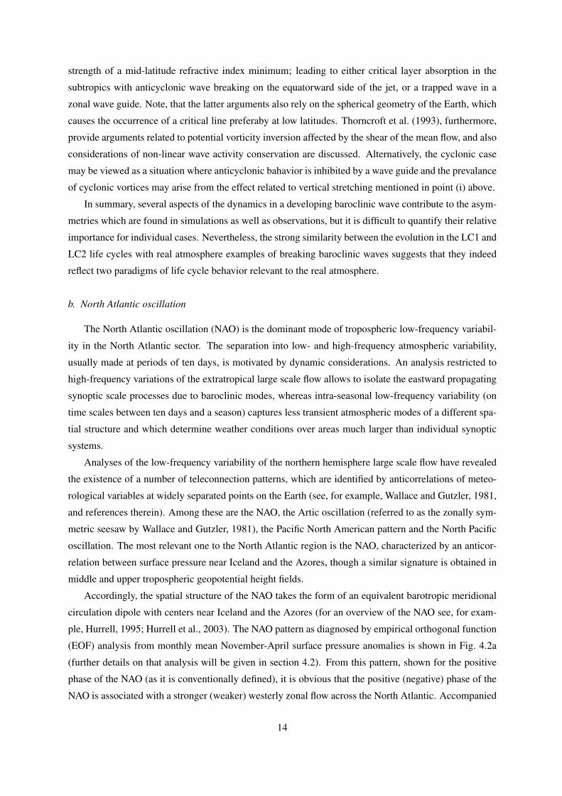
strength of a mid-latitude refractive index minimum; leading to either critical layer absorption in the

subtropics with anticyclonic wave breaking on the equatorward side of the jet, or a trapped wave in a

zonal wave guide. Note, that the latter arguments also rely on the spherical geometry of the Earth, which

causes the occurrence of a critical line preferaby at low latitudes. Thorncroft et al. (1993), furthermore,

provide arguments related to potential vorticity inversion affected by the shear of the mean flow, and also

considerations of non-linear wave activity conservation are discussed. Alternatively, the cyclonic case

may be viewed as a situation where anticyclonic bahavior is inhibited by a wave guide and the prevalance

of cyclonic vortices may arise from the effect related to vertical stretching mentioned in point (i) above.

In summary, several aspects of the dynamics in a developing baroclinic wave contribute to the asym-

metries which are found in simulations as well as observations, but it is difficult to quantify their relative

importance for individual cases. Nevertheless, the strong similarity between the evolution in the LC1 and

LC2 life cycles with real atmosphere examples of breaking baroclinic waves suggests that they indeed

reflect two paradigms of life cycle behavior relevant to the real atmosphere.

b. North Atlantic oscillation

The North Atlantic oscillation (NAO) is the dominant mode of tropospheric low-frequency variabil-

ity in the North Atlantic sector. The separation into low- and high-frequency atmospheric variability,

usually made at periods of ten days, is motivated by dynamic considerations. An analysis restricted to

high-frequency variations of the extratropical large scale flow allows to isolate the eastward propagating

synoptic scale processes due to baroclinic modes, whereas intra-seasonal low-frequency variability (on

time scales between ten days and a season) captures less transient atmospheric modes of a different spa-

tial structure and which determine weather conditions over areas much larger than individual synoptic

systems.

Analyses of the low-frequency variability of the northern hemisphere large scale flow have revealed

the existence of a number of teleconnection patterns, which are identified by anticorrelations of meteo-

rological variables at widely separated points on the Earth (see, for example, Wallace and Gutzler, 1981,

and references therein). Among these are the NAO, the Artic oscillation (referred to as the zonally sym-

metric seesaw by Wallace and Gutzler, 1981), the Pacific North American pattern and the North Pacific

oscillation. The most relevant one to the North Atlantic region is the NAO, characterized by an anticor-

relation between surface pressure near Iceland and the Azores, though a similar signature is obtained in

middle and upper tropospheric geopotential height fields.

Accordingly, the spatial structure of the NAO takes the form of an equivalent barotropic meridional

circulation dipole with centers near Iceland and the Azores (for an overview of the NAO see, for exam-

ple, Hurrell, 1995; Hurrell et al., 2003). The NAO pattern as diagnosed by empirical orthogonal function

(EOF) analysis from monthly mean November-April surface pressure anomalies is shown in Fig. 4.2a

(further details on that analysis will be given in section 4.2). From this pattern, shown for the positive

phase of the NAO (as it is conventionally defined), it is obvious that the positive (negative) phase of the

NAO is associated with a stronger (weaker) westerly zonal flow across the North Atlantic. Accompanied

14

FIG. 1.4 Idealized relationships between pressure and temperature anomalies associated with the North Atlantic oscillation

(after Wallace and Gutzler, 1981).

are these changes in the large scale flow by significant temperature changes during winter over the sur-

rounding continents. Specifically, during the positive phase of the NAO, temperatures in northern Europe

and the eastern U.S. are anomalously high while anomalously low over the Greenland-Labrador region

and the Middle East due to advection of maritime and continental air masses, respectively, as illustrated

schematically in Fig. 1.4, and vice versa for the negative phase of the NAO. It is this temperature seesaw

between Greenland and northern Europe, linked with North Atlantic surface pressure variations, that

prompted Walker and Bliss (1932) to term this phenomenon the North Atlantic oscillation; and its strong

influence on European and North American surface climate makes the NAO such an important mode of

low-frequency variability.

The variability of the NAO is largest on inter-annual time scales as seen, for instance, in the power

spectrum of the daily NAO index time series (defined by the projection coefficients of daily anomaly

fields onto the NAO pattern). This spectrum is explained at the 95% confidence level by a red noise

process with an autocorrelation e-folding time scale of about ten days, as shown by Feldstein (2000) —

and such a process has larger inter-annual than intra-seasonal variance. Additionally, this short character-

istic time scale (compared to that where the largest variance occurs) suggests that monthly or seasonally

averaged NAO anomalies do not reflect a steady response to a steady forcing over that period, but in-

stead represent the averaged response to an averaged forcing, both of which consist of much shorter time

scale fluctuations than a month or a season. In this picture, low-frequency (e.g., monthly or seasonal

mean) NAO anomalies may simply arise due to more or less frequent high-frequency forcing episodes

of a particular sign during a longer period. Thus, an analysis based on monthly or seasonally averaged

data should be expected to obscure the fundamental dynamics that drive the NAO, although the use of

averaged data will improve statistical significance of the NAO itself due to an increased signal-to-noise

ratio. In fact, several studies (e.g., Feldstein, 2003) provide evidence that the NAO is driven, to a large

extent, by high-frequency eddy fluxes from synoptic scale processes, though also low-frequency eddies

contribute to its growth and decay. The role of synoptic scale processes, in particular, that of synoptic

scale wave breaking, will be discussed further in the motivation (section 1.2) and throughout this thesis.

15

FIG. 1.5 NAO-like circulation dipole induced by anomalous meridional eddy vorticity fluxes. Thin arrows examplify anoma-

lous northward vorticity fluxes (driving a positive phase NAO-like circulation dipole), and thick arrows pointing to the right

(left) indicate the induced anomalous eastward (westward) circulation (after Vallis et al., 2004).

Basically, the link between synoptic scale processes and the NAO can be understood in terms of

fluctuating high-frequency eddy vorticity fluxes across the mid-latitude eddy-driven jet. If a zonally con-

fined region like that of the North Atlantic storm-track is exposed to anomalous northward eddy vorticity

fluxes, then a cyclonic (anticyclonic) circulation is induced on the poleward (equatorward) side of the

jet due to convergent (divergent) vorticity fluxes. Conversely, a meridional circulation dipole of oppo-

site polarity results from anomalous southward vorticity fluxes. This demonstrates how anomalous eddy

vorticity fluxes, caused by variations of mid-latitude baroclinic processes, drive meridional circulation

dipoles that closely resemble either phase of the NAO, as shown schematically in Fig. 1.5. This simple

picture of eddy-driven meridional circulation dipoles is illustrated explicitly by Vallis et al. (2004), where

high-frequency meridional eddy vorticity fluxes are parameterized by stochastic forcing of the barotropic

vorticity equation in a mid-latitude band and which locally result in NAO-like circulation dipoles, even

for a zonally uniform basic state and forcing. Consequently, it is suggested that the NAO reflects a lo-

cal manifestation of such NAO-like circulation dipoles at longitudes where synoptic scale eddy vorticity

fluxes are maximized, namely, in the North Atlantic storm-track region. Furthermore, this concept moti-

vates the term ’NAO-like circulation dipole’ which also applies to idealized model settings with a zonally

uniform basic state, in contrast to the NAO as a spatially fixed pattern within a zonally non-uniform flow.

c. Stratosphere–troposphere coupling

In the stratosphere the extratropical circulation during winter is characterized by the westerly polar

night jet with an average latitudinal position near 60 latitude and its maximum near the stratopause. At

these levels in the northern hemisphere zonal mean zonal wind speeds can sometimes exceed 100 ms−1

and local wind speeds near 200 ms−1 are occasionally observed. The primary origin of this jet are the

strong meridional gradients of radiative heating across the boundary of the polar night at those latitudes,

north of which absorption of short wave radiation by ozone does not take place and thus radiative cooling

is not balanced by diabatic heating. However, from a potential vorticity perspective (referring to a non-

16

rotating frame of reference) the middle and high latitude circulation in the wintertime stratosphere is

suggestive of a large scale vortex centered near the pole, rather than an isolated jet stream as it appears

in the Eulerian zonal mean framework. This stratospheric polar vortex is characterized by steep potential

vorticity gradients on the equatorward flank of the polar night jet and a more homogeneous potential

vorticity distribution in its interior as well as outside the vortex (see, for example, the potential vorticity

maps of the polar vortex in Fig. 1.1).

The large potential vorticity gradients on the vortex edge allow for vertical propagation of Rossby

waves from the troposphere, largely excited by the quasi-stationary ultra-long planetary wave patterns

near the tropopause. At stratospheric levels these waves strongly interact with the vortex, and this inter-

action can be described either by wave-vortex dynamics (for references see the literature cited at the end

of the discussion of stratospheric planetary wave breaking in section 1.1a) or, alternatively, by the trans-

formed Eularian mean framework (e.g., Andrews et al., 1987). Since on average there must be a sink of

planetary wave activity in the stratosphere (associated with Eliassen-Palm flux convergence), the waves

act to reduce the strength of the polar vortex or polar night jet, compared to a purely radiatively forced cir-

culation. Hence, the variability of tropospheric planetary waves excites variability in stratospheric wave

drag and, thus, variations in the strength of the polar vortex. The fact that only those planetary waves of

largest zonal scale (wavenumbers 1 to 3) can penetrate into the stratosphere (as shown by the Charney-

Drazin criterion; see Charney and Drazin, 1961; Andrews et al., 1987) explains the predominance of

coherent hemispheric scale variability in the stratosphere, compared to the more regional character of

tropospheric low-frequency modes as, for example, the NAO. Consequently, stratospheric variability is

dominated by variations in the strength of the polar vortex, which is measured by the northern annular

mode (NAM), defined as the first EOF of northern hemisphere low-frequency filtered geopotential height

anomalies at a given pressure level. Accordingly, the corresponding NAM patterns exhibit a near zonally

uniform structure, as seen in Fig. 4.2b for the 50 hPa NAM (further details on that analysis will be given

in section 4.2).

The tropospheric NAM has a larger zonally non-uniform component with its mid-latitude centers

of action confined to the North Atlantic and Pacific storm-track regions (see, for example, Baldwin and

Dunkerton, 1999, 2001), and its signature in surface pressure corresponds to the Arctic oscillation (AO;

see Ambaum et al., 2001). In the North Atlantic sector the pattern of the NAM/AO is very similar to

that of the NAO. And, in fact, several observational and modeling studies find a close relation between

the more zonally confined NAO and the NAM/AO which reflects coherent hemispheric scale variations

(Wallace, 2000; Ambaum et al., 2001; Vallis et al., 2004; Feldstein and Franzke, 2006). Furthermore, it

is suggested that the structure of the NAO is a dynamically more representative mode of variability than

that of the tropospheric NAM/AO in the sense that the hemispheric scale NAM/AO signature may arise

solely due to the method of statistical analysis, that is, an EOF analysis of hemispheric scale anomaly

fields.

Additionally, evidence exists that also in the context of dynamical stratosphere–troposphere coupling

the NAO is the most relevant variability mode in the troposphere, rather than the NAM. Specifically,

17

episodes of an anomalously weak stratospheric polar vortex at 10 hPa (as measured by the 10 hPa NAM)

are associated by a negative NAO-like response in surface pressure over a period of 60 days after the

weak vortex event onset, as shown by Baldwin and Dunkerton (2001). It also turns out from this and

related studies that on average negative anomalies of the stratospheric NAM originate at upper strato-

spheric levels and then migrate downward into the lower stratosphere where these anomalies persist for

about two months (if sufficiently strong weak vortex events are selected at 10 hPa), and also induce

the aforementioned NAO-like response in the troposphere. However, for an analysis of the downward

migration of stratospheric NAM anomalies into the troposphere it is more convenient to use the NAM

also at tropospheric levels to prevent any discontinuity at the tropopause. Fig. C.1 in appendix C shows

the NAM index time series during all the extended winter seasons (November-April) from 1957/58 to

2001/02 and from 1 hPa near the stratopause down to the surface (further details on that analysis will

be given in section 4.2). This illustrates the variability of the coupled stratosphere–troposphere sys-

tem during winter. Evidently, most stratospheric weak vortex events are followed by an anomaly in the

troposphere of the same sign.

Different mechanisms have been proposed in the literature for dynamical stratosphere–troposphere

coupling. Thompson et al. (2006) present evidence that part of the observed tropospheric response to

stratospheric zonal mean circulation anomalies can be explained by anomalous stratospheric planetary

wave drag, which induces a zonal mean secondary circulation that closes off in the planetary boundary

layer and, thus, drives near surface zonal wind anomalies. This analysis is motivated by the downward

control principle, studied extensively by, for example, Haynes et al. (1991). Ambaum and Hoskins (2002)

propose a hydrostatic/geostrophic adjustment process and show how a strengthened (weakened) strato-

spheric polar vortex acts to raise (lower) the arctic tropopause which, in turn, leads to vertical stretching

(contraction) of the high-latitude troposphere beneath and, thus, to an increased (decreased) cyclonic

rotation that projects onto the positive (negative) AO as well as NAO. The study of Perlwitz and Harnik

(2003), on the other hand, focuses on coupling through zonally non-uniform processes. Specifically,

upward propagating ultra-long planetary waves of tropospheric origin encounter different flow condi-

tions in the stratosphere and, consequently, are either absorbed or reflected back into the troposphere

where the waves may interfere and, thus, alter tropospheric planetary wave amplitudes and phases.

Note, that the positive (negative) phase of the NAO also reflects states of reduced (incrreased) quasi-

stationary planetary wave amplitudes in the North Atlantic sector. However, a number of observational

and modeling studies also suggests the possibility that stratospheric information is mediated to tropo-

spheric low-frequency modes through synoptic scale systems in the sense that they respond to variations

of the stratospheric flow conditions, such that associated synoptic eddy fluxes are systematically altered

(Baldwin and Dunkerton, 1999, 2001; Baldwin et al., 2003; Kushner and Polvani, 2004; Charlton et al.,

2004; Wittman et al., 2004, 2007; Gerber and Polvani, 2008). Then the aggregated effect of several

individual synoptic scale systems may strongly project onto the NAO.

As mentioned at the beginning of this chapter, an understanding of the dynamical coupling between

the stratosphere and troposphere is of particular interest for extended-range (intra-seasonal) tropospheric

18

weather forecasts due to the relatively long dynamical time scales in the stratosphere. Explicit observa-

tional evidence for different time scales of NAM related variability at various levels in the troposphere

and stratosphere is given by, for example, Baldwin et al. (2003). The longest autocorrelation e-folding

time scale of the NAM index time series is found during mid-winter just above the tropopause and attains

values near 30 days. In the middle stratosphere as well as in the troposphere the NAM exhibits shorter

time scales of about two weeks. However, during all other seasons middle stratospheric time scales are

longer than during mid-winter, while in the troposphere they are shorter. Thus, the tropospheric NAM

time scale maximizes at the same time as does the NAM in the lowermost stratosphere. Also the tro-

pospheric response to stratospheric weak vortex events, which originate at upper stratospheric levels as

mentioned above, occurs almost simultanously with the persistent negative NAM anomaly in the lower-

most stratosphere (Baldwin and Dunkerton, 2001; Gerber and Polvani, 2008).

Hence, these time scale considerations further support the proposed mechanism of stratosphere–

troposphere coupling through a direct modulation of synoptic scale systems by variations of the lower

stratosphric flow. Note, that synoptic scale disturbances of much smaller spatial scale than the quasi-

stationary planetary waves can penetrate only into the lower stratosphere. Since, moreover, low-frequency

anomalies of the NAO are driven, to a large extent, by synoptic scale processes (as detailed in sec-

tion 1.1b) which arise from baroclinic instability, it is of great interest to investigate the response of

baroclinic waves in the troposphere to lower stratospheric flow conditions.

1.2 Motivation and key questions

The NAO which represents the dominant mode of low-frequency variability in the North Atlantic

sector is driven, to a large extent, by high-frequency eddy fluxes due to synoptic scale processes, as

discussed in section 1.1b. Although studies like that of Feldstein (2003) or Vallis et al. (2004) highlight

the importance of high-frequency eddy fluxes for the growth and decay of the NAO, they do not pro-

vide any details on the associated synoptic evolution. To bridge this gap Benedict et al. (2004) compute

composites for either phase of the NAO of daily unfiltered tropopause charts, showing potential temper-

ature on the tropopause (i.e., θ on 2 PVU, very similar to IPV on the 320 K-isentrope as presented in

section 1.1a). This composite analysis exhibits the signature of anticyclonic (cyclonic) synoptic scale

wave breaking in the North Atlantic sector prior to and during the positive (negative) phase of the NAO.

Specifically, in this picture the positive phase comes along with two anticyclonic wave breaking (AB)

events, one over the U.S. and another one over the eastern North Atlantic, while for the negative phase

the evolution indicates a single cyclonic wave breaking (CB) event over the central North Atlantic. Con-

sequently, it is suggested that the different phases of the NAO are the remnants of breaking synoptic

scale Rossby waves in the North Atlantic storm-track region (for details on the structure and dynamics of

northern hemisphere storm-tracks, see Blackmon, 1976; Chang et al., 2002). However, the appearance

of either kind of wave breaking in the composite does not necessarily imply the suggested causal rela-

tionship. Hence, it will be necessary to explicitly determine the response of the NAO to synoptic scale

19

FIG. 1.6 Time series of the NAO index (NAOI) during January and February 1986. For details on the computation of the

NAOI time series see section 4.2c. Upward (downward) arrows mark Jan 08th and Jan 11th (Feb 12th and Feb 16th) which are

the days when the anticyclonic (cyclonic) wave breaking events discussed in section 1.1a (and shown in Figs. 1.2 and 1.3) are

observed.

Rossby wave breaking.

Individual examples of AB and CB events are indeed supportive of the suggested relation, as illus-

trated in Fig. 1.6. The figure shows the daily NAO index time series during January and February 1986,

together with the dates of those AB and CB events which are presented in section 1.1a (and in Figs. 1.2

and 1.3). The two AB events on January 08th and January 11th occur near the locations found in the

composite analysis of Benedict et al. (2004) (see Fig. 1.2) and are also associated with the strong rise of

the NAO index during those days. Conversely, the CB event on February 12th initiates the rapid amplifi-

cation of the negative NAO period over the subsequent four days and the event on February 16th helps to

maintain this anomaly, and both events occur over the central North Atlantic region. Further CB events

occur later during the second half of February and during the significant decrease of the NAO index at

the end of January and beginning of February, and further AB events can be found during the increase

of the NAO index just after January 15th (not shown). From this synoptic view point, positive (negative)

monthly or seasonal mean NAO anomalies may then arise simply due to more frequent AB (CB) events

during that period within the North Atlantic storm-track.

Furthermore, the NAO is known to shift into its positive (negative) phase when the stratospheric polar

night jet or polar vortex is anomalously strong (weak), as discussed in section 1.1c (with reference to, for

example, Baldwin and Dunkerton, 2001). In particular, the potential relevance of synoptic scale systems

for dynamical stratosphere–troposphere coupling was highlighted in that discussion. Accordingly, from

the above NAO–wave breaking view it is highly suggestive that a stronger (weaker) westerly flow in the

lower stratosphere that persists over several weeks may cause synoptic scale waves in the troposphere to

break preferably anticyclonically (cyclonically) and, thereby, induce a low-frequency signal in the NAO.

This motivates the following three key questions of this thesis, which will be addressed in the fol-

20

lowing chapters from a modeling (Q-1 and Q-2) as well as observational perspective (Q-3):

Q-1 Does synoptic scale anticyclonic (cyclonic) wave breaking drive meridional circulation dipoles

resembling the positive (negative) phase of the NAO?

Q-2 Does stronger (weaker) westerly flow in the lower stratosphere induce anticyclonic (cyclonic) wave

breaking in the troposphere?

Q-3 What explicit observational evidence does exist for the suggested stratosphere–wave breaking–

NAO connection?

1.3 Outline and structure of the thesis

The outline of this thesis is as follows: Chapter 2 is primarily concerned with key question Q-1.

Specifically, a method for the detection of anticyclonic and cyclonic synoptic scale wave breaking is

constructed and applied to forced-dissipative simulations with a simplified general circulation model,

using a zonally uniform basic state. While in that study Q-2 is only briefly addressed, it is the main

focus of chapter 3, where the response of idealized baroclinic wave life cycles to lower stratospheric

flow conditions is investigated. In particular, changes in life cycle behavior from LC1 (associated with

anticyclonic wave breaking) to LC2 (cyclonic wave breaking) are discussed, together with its relation

to the NAO. Explicit observational evidence for the suggested relation between synoptic scale wave

breaking, the NAO and the stratosphere (Q-3) is provided in chapter 4 by applying the wave breaking

detection method, introduced in chapter 2, to the ERA-40 reanalysis. Finally, a discussion of the results,

the conclusions and perspective follow in chapter 5.

Since the chapters 2 to 4 have been submitted separately as individual journal publications (and are

presented here in their first submitted version, beside some minimal changes to adjust cross references

among the chapters of this thesis), each of these chapters has its own abstract, introduction and clonclu-

sions section. By virtue of this structure each of these chapters represents a stand-alone unit and, thus, is

readable independently — though it is also associated with the effect that a few aspects appear repeatedly

throughout the whole thesis, in particular, in the introductions of chapter 2 to 4.

21

22

2 Synoptic scale wave breaking and its potential

to drive NAO-like circulation dipoles:

A simplified GCM approach

ABSTRACT

Recent studies suggest a synoptic view of the North Atlantic oscillation (NAO) with its positive (negative) phase

being the remnant of anticyclonic (cyclonic) synoptic scale wave breaking. This study examines the potential

of such wave breaking events alone (in the absence of a zonally non-uniform background flow and boundary

conditions) to drive NAO-like meridional circulation dipoles by investigating the synoptic evolution of anticyclonic

(AB) and cyclonic wave breaking (CB) events in a mid-latitude eddy-driven jet in a simplified GCM with zonally

uniform basic state. First, a method for the detection of AB and CB events from daily maps of isentropic potential

vorticity and horizontal deformation is constructed. Then, from the obtained large sample of wave breaking events

AB- and CB-composites of the upper and lower tropospheric flow are computed, and a distinct spatial and temporal

asymmetry in the response to AB and CB events is found. While from the interaction of two AB events (with a mean

lifetime of 2.6 days) a strong and short-lived positive phase NAO-like dipole is produced at the surface but not at

upper levels, single CB events (4.3 days) are found to drive a strong and more persistent negative phase NAO-like

dipole at upper levels but not at the surface. It is concluded that AB (CB) is not capable of driving a positive

(negative) phase NAO-like dipole individually. However, the results suggest that an equivalent barotropic NAO-

like variability mode may arise from the successive occurrence of AB and CB events. Further, a sensitivity to the

strength of the stratospheric polar vortex is found with more (less) frequent AB (CB) events under strong vortex

conditions.

2.1 Introduction

The North Atlantic oscillation (NAO) is the dominant mode of low-frequency variability (time scales

of 10 days and longer) over the North Atlantic in winter, and accounts for a significant fraction of variance

of European climate and weather (Hurrell, 1995; Hurrell et al., 2003). Although the NAO has significant

variability on inter-annual and longer time scales it has been shown that its intrinsic time scale is of the

order of 10 days (Feldstein, 2000, 2003), in the sense of both composite positive/negative phase NAO

23

events and the autocorrelation e-folding time scale of a daily NAO index. Consistently, the NAO is

driven, to a large extent, by high-frequency eddy fluxes, though also low-frequency eddies contribute

to its growth and decay (e.g., Feldstein, 2003). Nonetheless, other factors of much longer time scales

such as sea surface temperatures, tropical variability and influences from the stratosphere play a role for

inter-annual variability (Hurrell et al., 2003).

In the simplest picture, the dynamical process that drives the different phases of the NAO, that is, a

meridional circulation dipole of opposite vorticity anomalies appears to be fluctuating meridional eddy

vorticity fluxes by mid-latitude synoptic scale waves. A simple and illustrative model of this mechanism

is presented by Vallis et al. (2004), where high-frequency eddy vorticity fluxes are parameterized by

stochastic forcing of the barotropic vorticity equation in a mid-latitude band and which locally results

in NAO-like meridional circulation dipoles. Although this model captures the dynamical essence of

NAO-like variability, it is, certainly, only a crude approximation to the real atmosphere where a large

contribution to eddy vorticity fluxes comes from meridional wave propagation during the decay stage of

baroclinic waves, characterized by the occurrence of synoptic scale wave breaking (Riviere and Orlanski,

2007). From the synoptic view point of Benedict et al. (2004), Franzke et al. (2004) and Riviere and

Orlanski (2007), accounting for the much more complex nature of the real atmosphere, it is suggested that

the positive phase NAO emerges from anticyclonic synoptic scale wave breaking1 over North America

and the North Atlantic, while the negative phase NAO arises from cyclonic wave breaking over the

North Atlantic. Woollings et al. (2008) give a different interpretation of the positive (negative) phase

NAO being driven by less (more) frequent wave breaking at the tropopause.

The above studies suggest that the two kinds of synoptic scale wave breaking are capable of driving

NAO-like meridional circulation dipoles of opposite sign. In this context it is reasonable to ask whether

additional aspects of the North Atlantic storm-track other than the pure synoptic scale wave breaking,

such as a zonally non-uniform background flow, sea surface temperatures or tropical influences, are

essential for such wave breaking to merge in a pattern of either phase of the NAO. One possibility to

address this point is to investigate the response of the large scale flow to anticyclonic and cyclonic wave

breaking in the absence of these potential aspects. From this approach, we pose the main question of this

study: What is the potential of anticyclonic (cyclonic) wave breaking alone for driving positive (negative)

phase NAO-like circulation dipoles? To address this question a set of forced-dissipative simulations of a

mid-latitude eddy-driven jet is carried out with a simplified GCM, using a zonally uniform basic state. In

order to investigate the synoptic evolution of both kinds of wave breaking in the context of the generation

of NAO-like circulation dipoles a method for the detection of such events is first constructed.

Consequently, this paper is organized as follows: The model and the specific setup used for this study

is described in section 2.2. The wave breaking detection method is introduced in section 2.3. Section 2.4

presents composites of the wave breaking events detected from the model simulations, and also briefly

investigates the influence of the strength of the stratospheric polar vortex on tropospheric wave breaking1Anticyclonic and cyclonic wave breaking according to the LC1 and LC2 idealized baroclinic wave life cycle, respectively

(see, e.g., Thorncroft et al., 1993).

24

characteristics, since the NAO is known to depend also on stratospheric conditions (e.g., Baldwin et al.,

1994). Though a closer treatment of such stratospheric impacts is left to a subsequent study including

stationary planetary waves.

2.2 Model and experimental setup

a. Model

For the numerical experiments of this study we use the dry primitive equation model PUMA (Fraedrich

et al., 1998, 2005)2. Such simplified general circulation models provide a platform for a systematic anal-

ysis of the dynamics of planetary atmospheres under idealized conditions, with minimal computational

expenses allowing for sufficiently long model time series for statistical data analysis. Here, we use this

model with T42 spectral horizontal resolution, 30 σ-levels in the vertical, and a timestep of 15 minutes.

Nine model levels are located in the troposphere (equally spaced w.r.t. σ) and 21 levels above (equally

spaced w.r.t. lnσ) with the uppermost model level at about 112 km (as in Scinocca and Haynes, 1998, see

their Appendix, but with σtran = 0.223). Diabatic heating is represented by Newtonian relaxation towards

an equilibrium temperature with heating timescales of 5, 10, 15, 20, and 30 days on the five lowermost

model levels, respectively, and 40 days above. Rayleigh friction is applied to the three lowermost model

levels to account for frictional effects in the planetary boundary layer with damping timescales of 1.168,

1.759, and 3.562 days, corresponding to the Held and Suarez (1994) scheme. Further, a sponge layer is

introduced by applying Rayleigh friction to all levels above 0.5 hPa (as in Polvani and Kushner, 2002,

see their Appendix) to avoid spurious wave reflection at the model top and numerical instability due to

large amplitude gravity waves. Finally, the model employs horizontal 8th-order (∇8) hyperdiffusion with

a dissipation timescale of 6 hours on the smallest resolved scale.

b. Experimental Setup

Since this study focuses on the effect of synoptic scale wave breaking events on the background

flow, we integrate the model with zonally uniform forcing and boundary conditions to avoid any explicit

forcing of stationary planetary waves. The dynamical fields of the simulations are, therefore, statistically

independent of longitude. Four different simulations are carried out which differ only in the diabatic

forcing in terms of the equilibrium temperature in the winter polar stratosphere above 100 hPa. The

strength of the polar vortex is controlled by changing the vertical lapse rate γ in that region (see the

Appendix for an exact specification of the equilibrium temperature). One simulation is performed with

no polar vortex (Sim-0) and three further simulations with weak (Sim-1), medium (Sim-2) and strong

(Sim-3) vortex forcing, where γ = 0, 1, 2, 3 K/km, respectively. All other parameters are kept fixed. The

forcing is time-independent and represents perpetual northern winter conditions. For each simulation the

model is integrated over 30 years (10800 days) and the initial five years are discarded to exclude effects2Model code and users guide are freely available at http://www.mi.uni-hamburg.de/puma

25

FIG. 2.1 Equilibrium temperature (in K, left) and zonally and time averaged zonal winds (in ms−1, right) of the simulations

with no (Sim-0), weak (Sim-1), medium (Sim-2) and strong (Sim-3) stratospheric polar vortex (from top to bottom; using the

last 25 years each). Zonal winds are shown together with the θ = 320 K surface (thick line); and the thin dashed vertical line

marks 46N. Only the lower part of the model domain is shown.

from the model’s spin-up phase.

Fig. 2.1 shows the different equilibrium temperatures together with the corresponding time and

zonal mean zonal winds of the respective simulations. Clearly, the strengthened stratospheric polar

vortex is the main response to increased high-latitude stratospheric cooling. However, there are also

changes in the tropospheric circulation, specifically, a slight poleward shift of the mid-latitude eddy-

driven jet. This tropospheric response resembles that found by Polvani and Kushner (2002) and Kushner

and Polvani (2004), using a similar model and setup, and where it is suggested that a baroclinic response

in the troposphere essentially accounts for those changes. Our choice of the tropospheric and lower

26

stratospheric forcing, however, differs from those studies in the sense that it always produces an eddy-

driven jet at mid-latitudes, which is more suggestive of the dynamical state over the North Atlantic

in winter, compared to a jet at 30N in the North Pacific sector. Moreover, the simulated jet shifts

over almost the same latitudinal range (from 46N in Sim-0 to 49N in Sim-3) as does the observed

eddy-driven jet over the North Atlantic depending on the NAO (for reference see, e.g., Ambaum et al.,

2001, their Fig. 7). Recalling the conceptual background of this study, namely the investigation of the

relevance of synoptic scale wave breaking for the NAO, this appears as one advantage of the configuration

of our forcing. Finally, the subtropical jet at the edge of the Hadley cell is weak compared to the real

atmosphere, as it is often the case for simplified dry general circulation models due to the lack of tropical

moist convective variability. Hence, this model setup is optimal for the study of extratropical synoptic

scale wave breaking in a mid-latitude eddy-driven jet, excluding potential external factors like tropical

variability, sea surface temperatures or ultralong (wavenumber 1 to 3) quasi-stationary planetary waves.

2.3 Wave breaking detection method

The concept of Rossby wave breaking (McIntyre and Palmer, 1983, 1985) was first applied to ultra-

long planetary waves in the winter stratosphere. However, many studies are also concerned with breaking

synoptic scale Rossby waves near the tropopause during their barotropic decay stage, and its dynami-

cal relevance for the large scale tropospheric circulation (e.g., Thorncroft et al., 1993; Nakamura and

Plumb, 1994; Peters and Waugh, 1996; Esler and Haynes, 1999; Benedict et al., 2004; Abatzoglou and

Magnusdottir, 2006; Martius et al., 2007; Woollings et al., 2008), or mass/tracer transport between the

stratosphere and troposphere (e.g., Appenzeller and Davies, 1992; Waugh et al., 1994). Rossby wave

propagation ultimatively originates from background PV gradients which provide the restoring force for

the associated parcel oscillations. When such waves attain large amplitudes non-linear advection pro-

cesses come into play, leading to large horizontal parcel displacements and, eventually, to irreversible

mixing of PV. This can be seen best in the large scale overturning of isentropic PV contours near the

tropopause, indicating a local reversal of the PV gradient and, therefore, inhibiting further Rossby wave

propagation in that region. This reversed PV gradient is the essential dynamical aspect of breaking

Rossby waves, and, therefore, has been used in different studies for their detection (e.g., Abatzoglou

and Magnusdottir, 2006; Woollings et al., 2008). Our wave breaking detection method is also based

on this idea and introduced in the following together with a kinematic criterion for classification into

anticyclonically and cyclonically breaking waves.

a. Detection of a breaking wave

The method for the detection of breaking synoptic scale Rossby waves in the troposphere used in

this model study works as follows. First, daily maps of isentropic (Ertel’s) PV (IPV for short) on an

upper tropospheric isentropic surface are calculated, poleward of 20 latitude in the winter hemisphere.

We choose the θ = 320 K potential temperature surface, which is located between 400 hPa and 350 hPa

27

in the tropics and around 270 hPa at polar latitudes for this model setup (see Fig. 2.1). Then, on this θ-

surface an individual wave breaking event is, basically, defined as a two-dimensional horizontal structure

characterized by a reversed (i.e., negative) meridional IPV gradient, and is detected and tracked in time

by the following three steps:

Step 1 (search for meridional IPV reversal). At each longitude (of the corresponding Gaussian

model grid with 128 longitudes at T42) the meridional IPV profile is searched for reversals of the pole-

ward IPV gradient from positive to negative values. Specifically (see Fig. 2.2a for illustration), starting

from φ0 = 20N , the method looks for the latitude φmax of the first IPV maximum IPV (φmax). Next,

if φmax < 90N , the absolute IPV minimum north of φmax is searched, located at φmin. Finally, the

absolute IPV maximum between φmin and φmax is determined, IPV (φ′max).3 Now, if

IPV (φ′max)− IPV (φmin) > ∆IPV, (2.1)

with a prescribed threshold value ∆IPV , then this IPV reversal is said to belong to a wave breaking

event. If condition (2.1) is true for ∆IPV = ∆IPVdetect = 1 PVU, it is called a strong reversal, if

(2.1) is true only for ∆IPV = ∆IPVextend = 0.75 PVU it is called a weak reversal (where 1 PVU =

1 potential vorticity unit = 10−6s−1Km2kg−1). φ′max and φmin are the southern and northern bounds,

respectively, of this wave breaking event at the particular longitude, and correspond to the latitude of the

associated IPV trough and ridge, respectively. Subsequently, the same longitude is searched for further

IPV reversals at higher latitudes by iteration of step 1, starting from the northern bound of the previously

detected reversal, say, with φ0 = φmin.

Step 2 (longitudinal extension). Different IPV reversals found by step 1, which occur at neighboring

longitudes λ, are grouped together and taken as the same wave breaking event, if the difference in their

latitudinal position in terms of φmax is less than two gridpoints (∼ 5 latitude at T42), and if at least

one strong reversal is contained in this group. Note, that with ∆IPVdetect (2.1) becomes the necessary

condition for detection of an event, while with ∆IPVextend (2.1) becomes a sufficient condition for

longitudinal extension of an event. Now, individual wave breaking events consist of two-dimensional

horizontal IPV structures, characterized by an IPV trough-ridge-pair with anticyclonic IPV north of

cyclonic IPV ; and the wave breaking region is defined as the area within the longitude-latitude box

spanned by the westernmost and easternmost longitude of the event, and the southernmost point of the

IPV trough axis (given by φ′max) and the northernmost point of the IPV ridge axis (given by φmin). The

central point, (λc, φc), of an event is defined as the center of its wave breaking region.

Step 3 (time tracking). Two wave breaking events found by step 2, which occur on subsequent days,

are taken as the same event in case of spatial overlap of their wave breaking regions. See Fig. 2.2b for an

illustration of this tracking in time. Thus, each wave breaking event persists for a certain number of days

Nt. In order to exclude very short-lived events which only marginally fulfill the conditions for detection,

all events with Nt = 1 are discarded.

3Note, that φ′max may be equal to φmax.

28

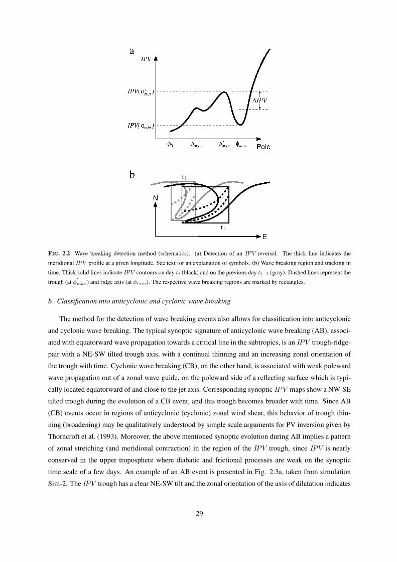
FIG. 2.2 Wave breaking detection method (schematics). (a) Detection of an IPV reversal. The thick line indicates the

meridional IPV profile at a given longitude. See text for an explanation of symbols. (b) Wave breaking region and tracking in

time. Thick solid lines indicate IPV contours on day ti (black) and on the previous day ti−1 (gray). Dashed lines represent the

trough (at φ′max) and ridge axis (at φmin). The respective wave breaking regions are marked by rectangles.

b. Classification into anticyclonic and cyclonic wave breaking

The method for the detection of wave breaking events also allows for classification into anticyclonic

and cyclonic wave breaking. The typical synoptic signature of anticyclonic wave breaking (AB), associ-

ated with equatorward wave propagation towards a critical line in the subtropics, is an IPV trough-ridge-

pair with a NE-SW tilted trough axis, with a continual thinning and an increasing zonal orientation of

the trough with time. Cyclonic wave breaking (CB), on the other hand, is associated with weak poleward

wave propagation out of a zonal wave guide, on the poleward side of a reflecting surface which is typi-

cally located equatorward of and close to the jet axis. Corresponding synoptic IPV maps show a NW-SE

tilted trough during the evolution of a CB event, and this trough becomes broader with time. Since AB

(CB) events occur in regions of anticyclonic (cyclonic) zonal wind shear, this behavior of trough thin-

ning (broadening) may be qualitatively understood by simple scale arguments for PV inversion given by

Thorncroft et al. (1993). Moreover, the above mentioned synoptic evolution during AB implies a pattern

of zonal stretching (and meridional contraction) in the region of the IPV trough, since IPV is nearly

conserved in the upper troposphere where diabatic and frictional processes are weak on the synoptic

time scale of a few days. An example of an AB event is presented in Fig. 2.3a, taken from simulation

Sim-2. The IPV trough has a clear NE-SW tilt and the zonal orientation of the axis of dilatation indicates

29

FIG. 2.3 Examples of an anticyclonic (AB, a) and cyclonic wave breaking event (CB, b), detected by the wave breaking

detection method on day 2433 and day 7001, respectively, of Sim-2. IPV at θ = 320 K is shown by contours and shading.

Contour interval is 0.5 PVU; solid contours are at 2, 2.5, 3 and 3.5 PVU; darker shading represents larger values. Isentropic

deformation is depicted by axes of dilatation; length of line segments indicates rate of deformation. Rectangles encircle grid

points of the strongest IPV reversal of the respective event, i.e., from (λmax, φ′max) to (λmax, φmin).

zonal stretching. During a typical CB event, on the other hand, we have meridional stretching (and zonal

contraction) in the region of the IPV trough, that makes this trough broader with time. The respective

example of a CB event (Fig. 2.3b) exhibits a NW-SE tilted trough and a meridional orientation of the

axis of dilatation.

We use these different characteristics of the deformation field to define a kinematic criterion to clas-

sify the detected wave breaking events into AB and CB. First, daily maps of isentropic horizontal stretch-

ing deformation

S =1

a cos φ

(∂u

∂λ− ∂

∂φ(v cos φ)

)(2.2)

are calculated for the same area and level as the IPV , where u and v are the isentropic zonal and

meridional wind components, respectively, and a the Earth’s radius. Positive (negative) S indicates zonal

(meridional) stretching. Next, for each individual wave breaking event that occurs on days t1, . . . , tNt

the initial stretching S1 = S(λmax, φ′max, t1) is determined. Here, (λmax, φ

′max) is that point on the

IPV trough axis with the maximum meridional IPV reversal IPV (φ′max) − IPV (φmin) (marked by a

rectangle in Fig. 2.3). Then, given a threshold value S?1 , a wave breaking event may be classified as

follows:

Wave breaking event is of type

AB, if S1 > S?

1

CB, if S1 < S?1

. (2.3)

Alternatively, to extract the most distinct AB and CB events from a set of wave breaking events for the

computation of AB- and CB-composites, two thresholds are defined by the upper (Q+) and lower (Q−)

quantiles of the S1 distribution, respectively:

Wave breaking event is used for

AB-composite, if S1 > S

Q+

1

CB-composite, if S1 < SQ−1

. (2.4)

For the composite analysis in the next section we choose the 15.9%-quantiles and, thus, there are 15.9%

of all events with S1 > SQ+1 and 15.9% with S1 < SQ−

1 .

30

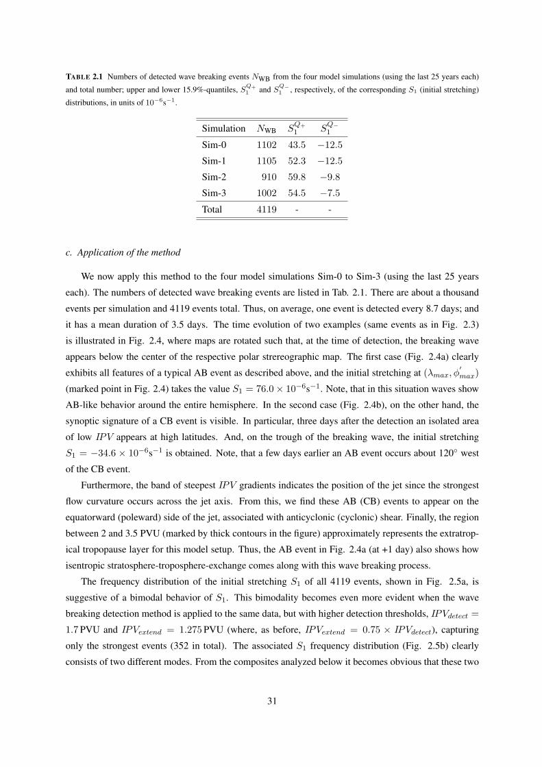
TABLE 2.1 Numbers of detected wave breaking events NWB from the four model simulations (using the last 25 years each)

and total number; upper and lower 15.9%-quantiles, SQ+1 and S

Q−1 , respectively, of the corresponding S1 (initial stretching)

distributions, in units of 10−6s−1.

Simulation NWB SQ+

1 SQ−1

Sim-0 1102 43.5 −12.5

Sim-1 1105 52.3 −12.5

Sim-2 910 59.8 −9.8

Sim-3 1002 54.5 −7.5

Total 4119 - -

c. Application of the method

We now apply this method to the four model simulations Sim-0 to Sim-3 (using the last 25 years

each). The numbers of detected wave breaking events are listed in Tab. 2.1. There are about a thousand

events per simulation and 4119 events total. Thus, on average, one event is detected every 8.7 days; and

it has a mean duration of 3.5 days. The time evolution of two examples (same events as in Fig. 2.3)

is illustrated in Fig. 2.4, where maps are rotated such that, at the time of detection, the breaking wave

appears below the center of the respective polar strereographic map. The first case (Fig. 2.4a) clearly

exhibits all features of a typical AB event as described above, and the initial stretching at (λmax, φ′max)

(marked point in Fig. 2.4) takes the value S1 = 76.0× 10−6s−1. Note, that in this situation waves show

AB-like behavior around the entire hemisphere. In the second case (Fig. 2.4b), on the other hand, the

synoptic signature of a CB event is visible. In particular, three days after the detection an isolated area

of low IPV appears at high latitudes. And, on the trough of the breaking wave, the initial stretching

S1 = −34.6 × 10−6s−1 is obtained. Note, that a few days earlier an AB event occurs about 120 west

of the CB event.

Furthermore, the band of steepest IPV gradients indicates the position of the jet since the strongest

flow curvature occurs across the jet axis. From this, we find these AB (CB) events to appear on the

equatorward (poleward) side of the jet, associated with anticyclonic (cyclonic) shear. Finally, the region

between 2 and 3.5 PVU (marked by thick contours in the figure) approximately represents the extratrop-

ical tropopause layer for this model setup. Thus, the AB event in Fig. 2.4a (at +1 day) also shows how

isentropic stratosphere-troposphere-exchange comes along with this wave breaking process.

The frequency distribution of the initial stretching S1 of all 4119 events, shown in Fig. 2.5a, is

suggestive of a bimodal behavior of S1. This bimodality becomes even more evident when the wave

breaking detection method is applied to the same data, but with higher detection thresholds, IPVdetect =

1.7 PVU and IPVextend = 1.275 PVU (where, as before, IPVextend = 0.75 × IPVdetect), capturing

only the strongest events (352 in total). The associated S1 frequency distribution (Fig. 2.5b) clearly

consists of two different modes. From the composites analyzed below it becomes obvious that these two

31

FIG. 2.4 Same examples of an AB (a) and CB event (b) as in Fig. 2.3. IPV at θ = 320 K (north of 20N) is shown by contours

and shading. Contour interval is 0.5 PVU; lowest contour is at 0.5 PVU; thick contours are at 2, 2.5, 3 and 3.5 PVU; darker

shading represents larger values. Cross symbols mark the point (λmax, φ′max) where the initial stretching S1 is evaluated.

Numbers are days relative to the time of detection.

modes are associated with anticyclonic and cyclonic wave breaking, confirming the usefulness of the

initial stretching S1 for classification into AB and CB. Also the S1 values of the above mentioned two

examples of an AB and CB event fall into the opposite tails of the frequency distribution. Note, however,

that for all further analysis the low detection thresholds IPVdetect = 1.0 PVU and IPVextend = 0.75 PVU

are used to obtain a larger sample of events. Although smaller detection thresholds further increase the

sample size, a large number of sub-synoptic scale IPV reversals is then included which are not the focus

of this study. Testing different values (not shown) we found the aforementioned detection thresholds to

32

FIG. 2.4 continued.

be a reasonable choice.

AB- and CB-composites of IPV are shown in Fig. 2.6a and b, taken on the first day of each event,

shifted in longitude and latitude in a way that the central point (λc, φc) of each event is located in the

center of the map (with relative longitude λrel = λ − λc and latitude φrel = φ − φc). Here, the events

are classified into AB and CB according to (2.3), with S?1 = 26 × 10−6s−1. This threshold roughly

separates the two modes in the S1 frequency distribution. Both, AB- and CB-composites, reveal the

typical synoptic signature of a thin NE-SW tilted trough for AB and a broad NW-SE tilted trough for CB

with the formation of a cut-off cyclone. These composites are compared to those calculated according

to (2.4), using the 15.9%-quantiles (Fig. 2.6c, d), and strong similarity between the respective patterns

is found. Note, that the quantiles are calculated for each simulation separately, and are listed in Tab.

33

FIG. 2.5 Frequency distribution of isentropic stretching deformation (in 10−6s−1) at the time of detection, S1 (initial stretch-

ing), of each wave breaking event, for (a) ∆IPVdetect = 1 PVU and (b) ∆IPVdetect = 1.7 PVU.

2.1. The according composites for the separate simulations (not shown) are very similar to the total

composites in Fig. 2.6 which our analysis is, thus, based on. Also for the remaining composite analysis

in the next section we only show composites calculated according to (2.4), since the two modes in

the S1 frequency distribution strongly overlap at intermediate values of S1 and, therefore, using (2.4)

for composite classification is cleaner. Though, all composites were also calculated using (2.3) and,

qualitatively, the same results are obtained.

FIG. 2.6 AB- (a, c) and CB-composites (b, d) of IPV at θ = 320 K (at the time of detection), using the threshold S?1 =

26× 10−6s−1 (a, b) and the 15.9%-quantiles SQ−1 and SQ+

1 (c, d) for classification into AB and CB. Contour interval is 0.125

PVU; thick contours are at 2, 2.5, 3 and 3.5 PVU. Coordinates are relative longitude and latitude.

2.4 Anticyclonic and cyclonic wave breaking

In this section we extend the previously described composite analysis to gain insight into the synoptic

evolution of the AB and CB events detected by our method, and to investigate its potential to drive NAO-

like meridional dipole patterns. Subsequently, the main results are quantitatively confirmed by studying

the impact of the two kinds of wave breaking on the annular mode, that is, the dominant dynamical mode

in the model. Finally, at the end of this section, we briefly discuss some differences in the wave breaking

statistics among the simulations with different stratospheric forcing.

34

a. Synoptic evolution of breaking waves

First, lagged AB- and CB-composites4 of IPV at θ = 320 K are presented (Fig. 2.7) to illustrate

the temporal evolution of the detected wave breaking events. Shown are IPV anomalies with respect to

the zonal mean at lag -14 days (lag -14 for short) when the respective composites are virtually zonally

uniform. Thus, anomalies in Fig. 2.7 represent the total change in the course of a wave breaking event,

including zonal mean changes. As before, composites are shown with relative longitude λrel and latitude

φrel. Each individual relative latitude φrel occurs for a certain number of wave breaking events N(φrel)

which can be smaller than the total number of events Ntot, since for some events a few relative latitudes

correspond to absolute latitudes φ beyond the north pole. Thus, composites are reliable only where

the ratio r(φrel) = N(φrel)/Ntot is close to one. This ratio is included in Fig. 2.7 by white (black)

shading where r = 1 (r = 0). The much smaller values of r at high relative latitudes in the CB-

composite compared to the AB case clearly indicate the more poleward ocurrence of CB events. This is a

consequence of the fact that CB events take place on the poleward side and AB events on the equatorward

side of the jet.

Both, the AB- and CB-composites show a wave group propagating eastward on the background

IPV gradient in the westerly jet, with a clear downstream development signature as it is typical for

Rossby waves. Moreover, these wave groups grow in amplitude as lag 0 is approached, as indicated

by the increasing isentropic north-south parcel displacement (or IPV contour undulation), and, conse-

quently, the waves become more and more affected by the meridionally varying background flow.

In the AB-composite, under the influence of anticyclonic background shear, the wave group shows

equatorward propagation, and, subsequently, the NE-SW tilted IPV trough of the detected wave breaking

event becomes zonally stretched and, eventually, quickly dissipates away. From this trough also a small

and short-lived cut-off low is produced by lag 2. This is often observed in the real atmosphere as well

as in idealized baroclinic wave life cycles during anticyclonic wave breaking events, and frequently

initiates cold-frontal cyclogenesis as mentioned by, e.g., Thorncroft et al. (1993) and investigated in

more detail by Thorncroft and Hoskins (1990). The northern part of this trough, however, travels further

downstream along the northern flank of the jet and also quickly dissipates. Note, that all other troughs

of this wave group also have a marked NE-SW tilt and thus the waves to the west of the breaking wave

undergo an evolution similar to that of the breaking wave itself as the center of the group passes by. In

particular, the trough immediately to the west of the detected trough is split (by lag 1) in qualitatively

the same manner as described above. This suggests that, in most individual cases, there is a percursory

wave breaking event to the west of the detected one (see Fig. 2.4a for an example) which, however,

does not fully develop as the center of the wave group progresses further eastward, in the sense that the

associated wave does not completely propagate to the equatorward side of the jet; as it is the case for the

finally detected major wave breaking event. This sequence of the successive occurrence of a precursory

and a major wave breaking event closely resembles the two anticyclonically breaking waves over North

America and the North Atlantic observed during the onset of the positive phase of the NAO (Benedict4AB- / CB-composite classification according to (2.4), with each composite including 655 events total.

35

FIG. 2.7 AB- (left) and CB-composite (right) of IPV anomalies (with respect to zonal mean at lag -14 days) from lag -6 days

to +6 days. Contour interval is 0.1 PVU, the zero contour is omitted, and dashed contours indicate negative values. Thick

contours show total IPV at 2, 2.5, 3 and 3.5 PVU. Coordinates are relative longitude and latitude. Relative latitudes which

occured for all (zero) events are shaded in white (black).

et al., 2004, see their Fig. 3). Also the occurrence of the precursory event at a slightly higher latitude is

in agreement with that observational study. In the course of the major wave breaking event, then, part of

the wave activity is deposited on the equatorward side of the jet near a critical line and, consequently, the

amplitude of the wave group reduces. Hence, no further AB-like wave breaking is found downstream of

the wavebreaking region.

36

In the according CB-composite, influenced by cyclonic background shear, the wave group shows

poleward propagation. From the NW-SE tilted IPV trough of the breaking wave a large scale cut-off low

emerges at lag 0 and the corresponding cyclonic IPV anomaly propagates further downstream along the

jet. This behavior is well known also from cyclonic wave breaking events in idealized baroclinic wave life

cycles. The most distinct feature of the cyclonically breaking event in the composite, however, appears to

be the large scale and quasi-stationary anticyclonic IPV anomaly at high relative latitudes, produced by

poleward advection of low IPV air. Moreover, this anomaly persists for about a week after the detection

of the event. Furthermore, it is worth mentioning that a meridional dipole pattern with anticyclonic

north of cyclonic IPV , being suggestive of the remnant of a blocking anomaly, is found in the wave

breaking region already four days before the wave breaks. When during the subsequent days the wave

group passes through that region, the wave breaking process appears to reinforce this preexisting pattern

by generation of the anticyclonic IPV anomaly, though the final anticyclonic anomaly occurs at sightly

higher relative latitudes. This reinforcement is seen even more clearly in geopotential height composites

discussed below (Fig. 2.8). Finally, in this composite neither the signature of NW-SE (or NE-SW) tilted

troughs is found outside the wave breaking region, indicating wave propagation within a zonal wave

guide on the eddy-driven jet, nor does any other CB-like wave breaking event occur. Hence, cyclonic

wave breaking appears as a more zonally localized process and, additionally, the results suggest that CB

events occur most likely in the region of a preexisting blocking pattern with an anticyclonic anomaly

poleward of the jet, which is associated also with diffluent background flow (see absolute IPV contours

at lag -4). These characteristics resemble the single cyclonically breaking wave over the North Atlantic

observed during the onset of the negative phase of the NAO (Benedict et al., 2004, see their Fig. 5), and

also captures some aspects known from simple models of positive synoptic eddy feedbacks on blocking

anticyclones (Shutts, 1983; Illary, 1984; Haines and Marshall, 1987; Frisius et al., 1998; Luo, 2005).

In summary, both AB- and CB-composites reveal the typical characteristics of anticyclonic and cy-

clonic synoptic scale wave breaking, respectively. We can further conclude that there is a distinct asym-

metry between our AB- and CB-composites, in agreement with findings from AB- and CB-like wave

breaking in idealized baroclinic wave life cycles. This asymmetry is characterized as follows: (i) While

in the AB case the breaking wave quickly dissipates, the CB event produces a quasi-stationary and per-

sistent anticyclonic anomaly at high relative latitudes. Accordingly, the average lifetimes of the events

detected by the method are 2.6 days for AB and 4.3 days for CB. (ii) The AB-composite shows equator-

ward propagation of the entire wave group, whereas in the CB case poleward wave propagation occurs

exclusively in a zonally confined region. (iii) CB-like wave breaking takes place preferably in a region

of a preexisting diffluent pattern in the background flow, while AB-events occur at an arbitrary longi-

tude. The two latter points are consequences of the tendency to equatorward wave propagation due to

the Earth’s spherical geometry (e.g., Whitaker and Snyder, 1993) and also of the fact that wave breaking

is generally facilitated by diffluent background flows (e.g., Peters and Waugh, 1996). Hence, the CB-

composite reflects a situation where anticyclonic wave breaking is inhibited by a zonal wave guide, and

isolated cyclonic wave breaking is triggered locally by background diffluence in the jet exit to the west

37

of a preexisting blocking pattern.

b. Upper and lower tropospheric flow evolution

Next, the upper tropospheric large scale flow evolution during AB and CB events is illustrated by

composites of 300 hPa geopotential height, z300, anomalies (Fig. 2.8). Not surprisingly, similar struc-

tures are found as in the IPV composite for the upper tropospheric θ-surface. Nonetheless, some sys-

tematic differences exist due to the scale dependent relation between PV and geopotential height and the

latitudinal dependence of the Coriolis parameter coupling the large scale flow to the height field.

In the AB-composite the anticyclonic and cyclonic IPV anomalies have almost the same magnitude

at lag 0 and 1 (Fig. 2.7), whereas in the corresponding z300 composite (Fig. 2.8) the larger scale an-

ticyclone has a larger amplitude than the corresponding smaller scale trough and dominates the upper

tropospheric flow. Furthermore, the northern part of the trough of the precursory wave breaking event

is emphasized in the geopotential height field and appears as a distinct cyclonic anomaly through lag

2. This cyclonic anomaly of the precursory wave breaking event is advected north- and eastward by

the circulation around the strong anticyclonic anomaly of the major wave breaking event and, thus, a

meridional dipole pattern emerges after lag 0, resembling the observed evolution during the onset of

the positive phase of the NAO (Benedict et al., 2004). Since, however, in our AB-composite also the

cyclonic anomaly of the major wave breaking event is advected around the anticyclonic anomaly south-

and westward, a tripole pattern is eventually produced rather than a clear positive phase NAO-like dipole

pattern.

In the related CB-composite the anticyclonic anomaly at high relative latitudes (at zero relative lon-

gitude and negative lags) is more evident and, thus, the above mentioned reinforcement of the preexist-

ing blocking pattern by the cyclonically breaking wave is seen more clearly in the geopotential height

anomalies, than in the IPV composite. This pattern closely resembles a stationary negative phase NAO-

like dipole. Note, that the anticyclonic pole consists of a single stationary anticyclonic anomaly poleward

of the jet, whereas the cyclonic pole is accounted for by eastward propagating cyclonic anomalies within

the eddy-driven jet.

Finally, composites of surface pressure anomalies are shown since significant differences are to be

expected between the upper and lower tropospheric large scale flow during baroclinic wave breaking

processes (Fig. 2.9). In the AB-composite at negative lags and western relative longitudes the cyclonic

(anticyclonic) surface pressure anomalies propagate to higher (lower) latitudes during the life cycle of

each individual wave as the wave group progresses eastward, reflecting the equatorward mass shift across

the jet; as a consequence of the jet acceleration by eddy momentum fluxes caused by NE-SW tilted waves

on its equatorward flank. Furthermore, since the eastward Rossby wave group velocity exceeds the phase

velocity but also has an equatorward component, the corresponding anticyclones appear at successively

lower latitudes as the wave group propagates to the equatorward side of the jet, where finally the major

wave breaking event takes place and from which a strong positive phase NAO-like meridional surface

pressure dipole emerges at lag 1. The south-eastern and southern flank of the associated anticyclones

38

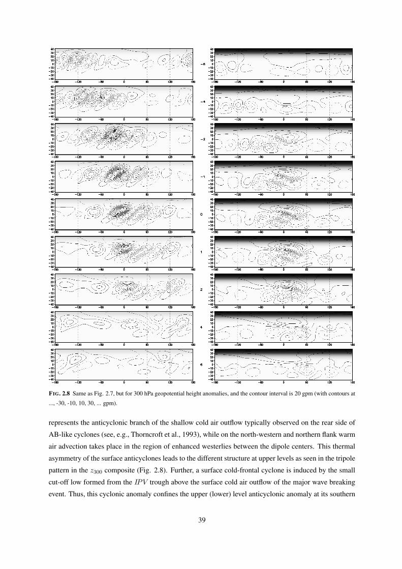
FIG. 2.8 Same as Fig. 2.7, but for 300 hPa geopotential height anomalies, and the contour interval is 20 gpm (with contours at

..., -30, -10, 10, 30, ... gpm).

represents the anticyclonic branch of the shallow cold air outflow typically observed on the rear side of

AB-like cyclones (see, e.g., Thorncroft et al., 1993), while on the north-western and northern flank warm

air advection takes place in the region of enhanced westerlies between the dipole centers. This thermal

asymmetry of the surface anticyclones leads to the different structure at upper levels as seen in the tripole

pattern in the z300 composite (Fig. 2.8). Further, a surface cold-frontal cyclone is induced by the small

cut-off low formed from the IPV trough above the surface cold air outflow of the major wave breaking

event. Thus, this cyclonic anomaly confines the upper (lower) level anticyclonic anomaly at its southern

39

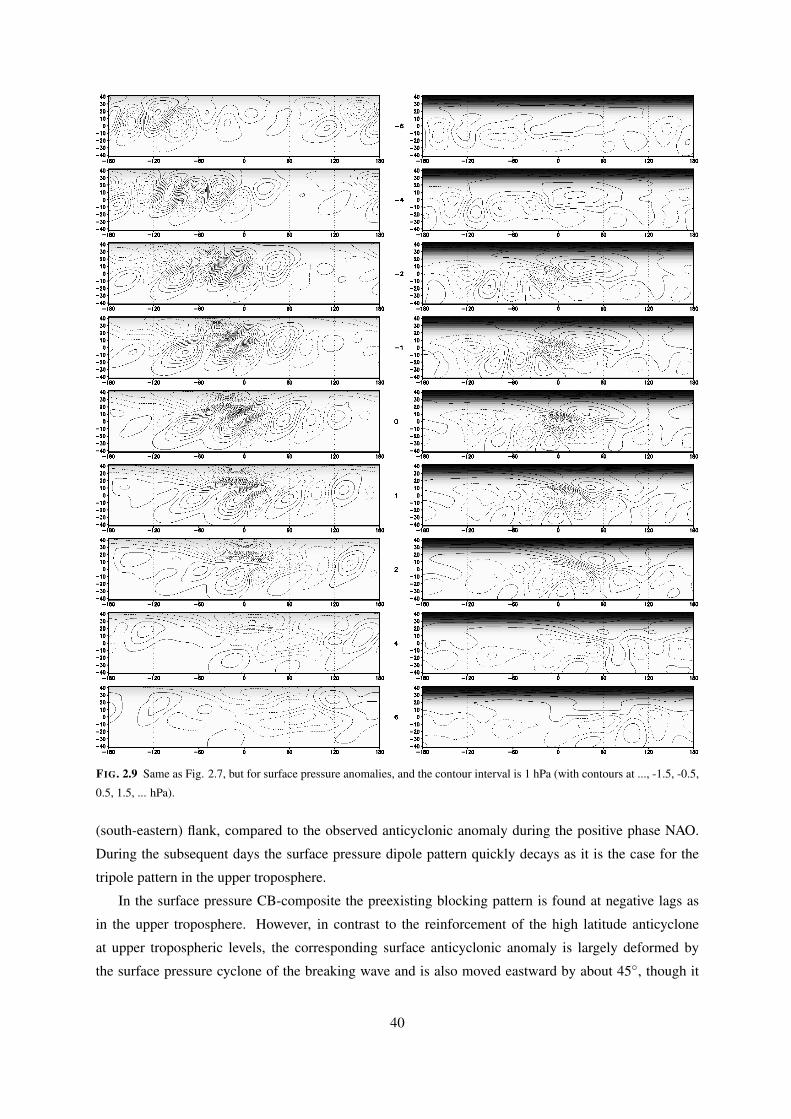
FIG. 2.9 Same as Fig. 2.7, but for surface pressure anomalies, and the contour interval is 1 hPa (with contours at ..., -1.5, -0.5,

0.5, 1.5, ... hPa).

(south-eastern) flank, compared to the observed anticyclonic anomaly during the positive phase NAO.

During the subsequent days the surface pressure dipole pattern quickly decays as it is the case for the

tripole pattern in the upper troposphere.

In the surface pressure CB-composite the preexisting blocking pattern is found at negative lags as

in the upper troposphere. However, in contrast to the reinforcement of the high latitude anticyclone

at upper tropospheric levels, the corresponding surface anticyclonic anomaly is largely deformed by

the surface pressure cyclone of the breaking wave and is also moved eastward by about 45, though it

40

undergoes temporary amplification. Thus, there is no negative phase NAO-like surface pressure dipole

generated by the CB event, unlike the upper tropospheric evolution. This surface pressure response is

again understandable in terms of eddy momentum fluxes which (as for the anticyclonically breaking

wave) locally accelerate the eastward zonal flow of the jet caused by the NW-SE tilted wave on its

poleward flank. The resulting equatorward mass shift across the jet again leads to a negative (positive)

surface pressure tendendy on the poleward (equatorward) flank of the jet (see lag -4 to lag 1 at zero

relative longitude). The warm air advection on the leading edge (north-eastern flank) of the surface

cyclone, however, helps to reinforce the upper tropospheric anticyclone above.

Summarizing this upper and lower tropospheric large scale flow evolution during AB and CB events

we have shown that anticyclonic wave breaking as detected by our method drives a distinct positive

phase NAO-like meridional circulation dipole at the surface but a different and more complex structure

in the upper troposphere, while cyclonic wave breaking drives (and reinforces) a negative phase NAO-

like dipole in the upper troposphere but not at the surface. Also the respective patterns of the response

to AB events do not resemble those from CB events with opposite sign due to the distinct asymmetry

between the dynamical evolution of AB and CB. And, furthermore, the respective response to cyclonic

wave breaking appears to be more persistent than the response to anticyclonic wave breaking.

Hence, if the two kinds of wave breaking are, conceptually, thought to drive the different phases of

the NAO, their respective contributions should lead to a threefold asymmetry of the NAO, specifically, in

the horizontal, the vertical and in the temporal component. Observational evidence is given by Blessing

et al. (2005). They find a temporal asymmetry between the two phases of the NAO with an average

lifetime (daily NAO index above plus (below minus) one standard deviation of a principle component

time series) of 3.3 days (4.5 days) for the positive (negative) phase. Any horizontal spatial asymmetry

is naturally excluded by the conventionally used linear methods (EOF or correlation analysis) to define

NAO indices, which are always based on a fixed spatial pattern.

Concerning the asymmetry in the vertical component it is important to note, that the resultant vari-

ability patterns at either level would indeed have an NAO-like character if a zonally confined region were

alternately forced by a lower tropospheric positive phase NAO dipole and an upper tropospheric negative

phase NAO dipole. Consequently, our results suggest the following idealized picture of an equivalent

barotropic NAO variability mode being driven by the successive occurrence of AB and CB (see Fig. 2.10

for an illustration). After baroclinic waves complete their growth stage in a baroclinically unstable state

of the eddy-driven jet, characterized by upward wave propagation and strong vertical wind shear, a more

barotropic state is driven during the barotropic decay stage of the waves by synoptic scale wave breaking,

associated with meridional wave propagation. This more barotropic state reflects the positive or nega-

tive phase of the NAO depending on whether the wave breaks anticyclonically or cyclonically. Either

phase of the NAO is maintained by subsequent wave breaking of the same kind, whereas the NAO phase

changes sign when a subsequent baroclinic wave life cycle results in wave breaking of the opposite kind.

This implies that the difference between the respective patterns driven by AB and CB (thick lines in Fig.

2.10) may account for NAO-like variability rather than the individual responses. Certainly, additional

41

FIG. 2.10 Schematic of equivalent barotropic NAO variability driven by AB (CB) at lower (upper) tropospheric levels. Merid-

ional profile of geopotential height z representing an NAO dipole at 1000 hPa and 300 hPa, and vertical profile of zonal wind

u between 1000 hPa and 300 hPa at latitude of maximum zonal winds φM . From a baroclinically unstable state (circles),

supporting baroclinic growth, either the positive (thick solid) or negative (thick dotted) NAO phase is driven by AB or CB,

respectively, during the barotropic decay stage of a baroclinic life cycle. The time mean is represented by thin dashed lines.

investigations are necessary to further refine this highly idealized picture of the positive (negative) phase

of the NAO being driven at lower (upper) levels. Specifically, a similar AB- and CB-composite analysis

from zonally non-uniform simulations including an NAO-like variability mode at a fixed location or from

observational data would allow for a close examination of these aspects by projecting the AB and CB

responses onto the corresponding variability pattern.

Clearly, in the real atmosphere diffluent background flow by the quasi-stationary waves in the North

Atlantic storm-track region is an important additional factor which favours and therefore localizes syn-

optic scale wave breaking there. Franzke et al. (2004) report that AB- and CB-like wave breaking in their

model only occurs in the right location to drive NAO-like variability if a realistic zonally non-uniform

basic state is chosen. However, still large case to case variability among individual wave breaking events

is observed even in a localized storm-track. Thus, small scale structures of the composite wave breaking

patterns (Figs. 2.7 to 2.9) would be smoothed out when averaging (in absolute longitude and latitude) a

large ensemble of such events taking place in the North Atlantic storm-track region.

c. Further remarks: North Atlantic storm-track region

To conclude our synoptic interpretation, we may hypothesize to what extent other factors of the

real North Atlantic storm-track region could modulate the response to anticyclonic and cyclonic wave

breaking. First, in the AB-composite the upper tropospheric flow does not closely resemble the positive

phase of the NAO due to the presence of the small cut-off low from the trough of the major wave breaking

event (see lag 1 and lag 2). In a typical North Atlantic setting, however, this positive IPV anomaly would

be close to the onset of the subtropical jet over the eastern North Atlantic which can be expected to move

that anomaly eastward and, thus, to allow for further southward extension of the dominant anticyclone

at upper levels, inducing a more positive phase NAO-like pattern. Additionally, the northern cyclonic

anomaly (from the precursory wave breaking event) might profit from the cold air reservoirs over Canada

42

and Greenland in the sense that it is deepened by low level cold air advection.

And, second, in the CB case the upper tropospheric negative phase NAO-like pattern induced (and re-

inforced) by the cyclonically breaking wave might largely trigger zonally smaller scale blocking episodes

over the same region, producing a significant negative phase NAO-like response at lower levels and the

surface. Shabbar et al. (2001) present observational evidence of increased occurrence of North Atlantic

blocking during the negative phase NAO, and Woollings et al. (2008) suggest an interpretation of the

positive (negative) phase NAO being essentially the result of less (more) frequent blocking episodes.

Their wave breaking index was indeed originally introduced as a blocking index by Pelly and Hoskins

(2003). This suggests that their index captures a combination of CB events (in the light of baroclinic

wave life cycles) and stationary blocking dipoles (in the sense of, e.g., Shutts, 1983) of smaller indi-

vidual zonal scale than the negative phase NAO pattern itself. For individual real synoptic situations it

might even be impossible to distinguish between these two concepts stemming from highly idealized

model approaches. Note, that the strong forcing of positive phase NAO-like dipoles at the surface by

anticyclonic wave breaking, however, is not made explicit by the Woollings et al. (2008) view.

d. Response of the annular mode

The zonally uniform forcing and boundary conditions of our model setup preclude the occurrence

of any NAO-like variability mode at a zonally fixed location and, therefore, the quantitative analysis

of its response to wave breaking events. However, observational and modeling evidence exists for the

NAO being a zonally confined manifestation of the same dynamical processes that drive hemispheric

scale variability modes like the Arctic oscillation or the annular mode (Wallace, 2000; Ambaum et al.,

2001; Vallis et al., 2004; Feldstein and Franzke, 2006). Thus, it is also reasonable to investigate the

response of the annular mode to anticyclonic and cyclonic wave breaking. For this purpose the surface

annular mode index (surface AMI) is calculated for each simulation separately by projection of daily

zonal mean surface pressure fields (north of 20N) onto the first EOF pattern of monthly and zonal mean

surface pressure fields. Accordingly, the 300 hPa AMI is constructed in the same way from 300 hPa

geopotential height fields. Both indices are normalized by its standard deviation. The corresponding

meridional annular mode structures are characterized by a maximum between 46N (Sim-0) and 49N

(Sim-3) and minimum values north of 70N. Then, lagged AB- and CB-composites of the surface and

the 300 hPa AMI are calculated, and shown in Fig. 2.11.

Evidently, anticyclonic (cyclonic) wave breaking induces a significant positive (negative) response

of the AMI, both at lower and upper tropospheric levels. The AMI peaks at lag 1 (lag 3) for AB (CB)

and attains a value of 0.80 (-0.39) at the surface and 0.70 (-0.80) at 300 hPa. These results confirm the

asymmetry of the response to AB and CB events in the temporal component and between lower and

upper levels. While the surface AMI AB-composite exceeds, for example, 0.6 for only three days (lag

0 to lag 2), the 300 hPa AMI CB-composite is less than -0.6 for eight days (lag 0 to lag 7). For smaller

absolute threshold values this temporal asymmetry is even more pronounced. Furthermore, the surface

AMI CB-composite shows that cyclonic wave breaking rather ineffectively drives the negative phase of

43

FIG. 2.11 AB- and CB-composites (see labels) of the annular mode index at the surface (black lines) and at 300 hPa (gray

lines). Thick lines indicate statistical significance at the 99.9% level.

the annular mode at lower levels, in accordance with the finding that CB events do not produce a clear

negative phase NAO-like dipole at the surface. However, the corresponding difference between the 300

hPa AMI AB-composites compared to that at the surface is smaller, although the synoptic signature of

AB events at upper levels does not closely resemble the positive phase NAO. That this is due to the wider

hemispheric extent of the AB signature at the peak time of the AMI can be seen in the respective AB-

and CB-composites of surface pressure and 300 hPa geopotential height, with respect to the time mean

(Fig. 2.12), now using absolute latitude and relative longitude. The 300 hPa AB-composite again (as

in Fig. 2.8) exhibits a tripole pattern but large amplitude anticyclonic anomalies at mid-latitudes appear

around the entire hemisphere (Fig. 2.12a), whereas the surface CB-composite (Fig. 2.12d) shows only

weak cyclonic anomalies outside the wave breaking region, consistent with the more zonally confined

nature of CB events.

It should also be mentioned that these composites reveal different dominant zonal wave numbers,

with zonal wave number five for AB (see Fig. 2.12a) and wave number six for CB (see Fig. 2.12b). This

is consistent with the result from idealized baroclinic wave life cycles that AB- (CB-) like behaviour is

favoured for longer (shorter) synoptic waves (Hartmann and Zuercher, 1998; Orlanski, 2003; Wittman

et al., 2007), and with the study by Riviere and Orlanski (2007) who force a high-resolution model over

the North Atlantic domain with observational data. Finally, we do not further interpret the weak but

statistically significant AMI response to AB and CB at positive lags beyond about 10 days since this is

likely to reflect the spurious and unrealistically long annular mode (decorrelation) time scale, which is

typically found in simplified GCMs as the one used in this study (Gerber et al., 2007)5.5The autocorrelation functions of the surface pressure AMI of our simulations have an e-folding time scale of 30 to 40 days,

while in the real atmosphere time scales of order two weeks are observed.

44

FIG. 2.12 AB- (a, c) and CB-composites (b, d) of 300 hPa geopotential height (a, b) and surface pressure (c, d) anomalies

(with respect to the time mean) at lag +1 day for AB- and +3 days for CB-composites. Contour intervals are the same as in Fig.

2.8 and Fig. 2.9. Coordinates are relative longitude and absolute latitude. Latitude circles are plotted at 0, 20, 40 and 60N.

e. Influence of the stratosphere

As mentioned in section 2.2 the tropospheric eddy-driven jet shifts poleward as the stratospheric

polar vortex is strengthened by diabatic cooling (Sim-0 to Sim-3). From the results of Polvani and

Kushner (2002) and Kushner and Polvani (2004) it is highly suggestive that this jet shift arises from

a baroclinic wave (or high-frequency synoptic scale) response in the troposphere projecting onto an

internal tropospheric mode of variability which is characterized by meridional vacillation of the zonal

mean eddy-driven jet (and is often associated with the tropospheric annular mode). This is particularly

plausible since many observational and modeling studies indicate a strong interaction between mid-

45

FIG. 2.13 Distributions of isentropic stretching deformation (in 10−6s−1) at the time of detection, S1 (initial stretching), of

each wave breaking event from Sim-0 (thick solid), Sim-1 (thin solid), Sim-2 (thin dashed) and Sim-3 (thick dashed), and the

difference Sim-0 minus Sim-3 (dotted).

latitude high-frequency eddies and the tropospheric zonal mean zonal flow in the sense of a positive

feedback that helps to maintain zonal flow anomalies by altered eddy propagation characteristics (e.g.,

Yu and Hartmann, 1993; Hartmann and Lo, 1998; Esler and Haynes, 1999; Lorenz and Hartmann, 2001).

In this eddy–zonal flow interaction framework the eddy feedback on the jet arises from eddy momen-

tum fluxes associated with anomalous equatorward (poleward) high-frequency eddy propagation during

a high (low) latitudinal position of the jet. It is, therefore, reasonable to ask whether this tendency to

more equatorward (poleward) wave propagation in the presence of a higher (lower) latitudinal position

of the jet is also reflected in our wave breaking statistics of the different simulations by more frequent

AB (CB) events under a stronger (weaker) stratospheric polar vortex.

For this purpose we compare the distributions of the initial stretching S1 of the different simulations

(Fig. 2.13). The fraction of wave breaking events with small S1 is largest for Sim-0 and reduces when

the polar vortex is strengthened in Sim-1, Sim-2 and Sim-3, indicating more (less) frequent AB- (CB-)

like behavior for a higher latitude tropospheric jet, below a stronger stratospheric jet. This is consistent

with the observational result that the positive phase of the NAO as well as the Arcitc Oscillation/annular

mode is favoured under strong stratospheric polar vortex conditions (Baldwin et al., 1994; Thompson and

Wallace, 1998; Baldwin and Dunkerton, 1999). Furthermore, the change of the ratio of the numbers of

AB- to CB-like events is maximized, if the separation is made at S?1 = 26× 10−6s−1. In section 2.3 this

was shown to be a reasonable threshold value to distinguish between AB- and CB-like wave breaking

(Fig. 2.6a, b) since it roughly separates the two modes in the S1 frequency distribution (Fig. 2.5). The

ratio then changes by 17% from Sim-0 to Sim-3 (see dotted line in Fig. 2.13).

Clearly, from this analysis it remains undecidable whether the stratospheric signal is mediated to

the troposphere by direct modulation of tropospheric baroclinic waves penetrating into the lowermost

46

stratospheric flow or by a zonal mean secondary circulation response to changed stratospheric wave

forcing that induces the tropospheric jet shift which in turn influences the baroclinic waves and thus the

synoptic scale wave breaking characteristics. However, the possibility of a direct response of baroclinic

waves to lowermost stratospheric flow conditions is suggested by several modeling studies (Polvani

and Kushner, 2002; Charlton et al., 2004; Kushner and Polvani, 2004; Wittman et al., 2004, 2007, and

chapter 3 of this thesis).

2.5 Discussion and conclusions

This idealized model study investigates the potential of synoptic scale anticyclonic and cyclonic

wave breaking alone for driving the different phases of the NAO. A method for the detection of such wave

breaking events is introduced and applied to four 25 years forced-dissipative simplified GCM simulations

with perpetual northern winter conditions and zonally uniform forcing and boundary conditions.

The wave breaking detection method is based on the identification of reversals of the meridional

IPV gradient, and the horizontal stretching deformation field is used to classify the detected events into

AB and CB. However, the chaotic nature of isentropic mixing due to mid-latitude synoptic eddies leads

to a large variety of spatial IPV patterns and, thus, many individual cases of wave breaking events

exhibit a signature with aspects of both AB and CB behavior. Nevertheless, for strong IPV reversals

clear bimodality is found, suggesting that the concept of AB- and CB-like wave breaking, motivated by

highly idealized adiabatic and frictionless baroclinic wave life cycle simulations with prescribed zonal

wave number, is indeed also relevant for the case of wave groups in a forced-dissipative setup.

The long model time series (1200 months total) allows for composite analysis of only the most dis-

tinct AB and CB events (tails of S1 frequency distribution). This immediately rises the question of the

applicability of the method to observational data, say, reanalysis products (nowadays spanning over about

50 years), where the sample size is largely reduced to the order of 150 winter months. If, additionally,

the analysis is confined to the North Atlantic sector, the expected number of wave breaking events is

much less than 10% of the corresponding number in this study (4119 events total). Furthermore, the

higher complexity of the real atmosphere flow due to stationary waves and also phenomena of smaller

than the resolved scales in our model are expected to increase the case to case variability of wave break-

ing events, even if those fields are interpolated to T42 resolution. Nevertheless, the actual presence of

frequent and clear AB- and CB-like signatures in observational tropopause charts and the appearance

of anticyclonically and cyclonically breaking waves even in a composite analysis of the NAO (Benedict

et al., 2004) are promising for the successful application of the method to real atmosphere data, for the

study of the effect of AB and CB events on low-frequency variability modes like the NAO or the Pacific

North American (PNA) pattern.

The advantage of the idealized model setup used here, however, is the possibility to investigate the

synoptic evolution of wave breaking in the absence of a stationary wave field, influences from the tropics

or the surface. For this purpose AB- and CB-composites were presented. Regarding the question posed in

47

section 2.1 of the potential of anticyclonic (cyclonic) wave breaking alone for driving positive (negative)

phase NAO-like circulation dipoles we can draw the following main conclusions from our composite

analysis:

• AB events are typically preceded by a precursory AB event (downstream development), resem-

bling the evolution during the onset of the positive phase of the NAO, while cyclonic breaking oc-

curs as a single CB event, as observed during the onset of the negative phase of the NAO (Benedict

et al., 2004), and is preferably triggered by a preexisting blocking (or negative phase NAO-like)

pattern.

• AB events drive strong positive phase NAO-like dipoles at the surface but not at upper tropospheric

levels due to the complex interaction of the precursory and the major wave breaking event6, while

CB events generate strong negative phase NAO-like dipoles at upper levels but not at the surface.

• AB events are short-lived processes (average lifetime 2.6 days), while CB events persist for longer

(4.3 days). This is true also for the response of the large scale flow (see previous point) and, thus,

consistent with the observed asymmetry in the temporal component of the NAO (Blessing et al.,

2005).

Hence, anticyclonic (cyclonic) synoptic scale wave breaking is not capable of driving full positive

(negative) phase NAO-like dipoles individually. Since, however, alternate forcing of a positive phase

NAO-like dipole at the surface and a negative phase NAO-like dipole at upper levels would indeed gen-

erate NAO-like variability at either level, our results suggest that the successive occurrence of AB and

CB events may drive an equivalent barotropic NAO-like variability mode in the troposphere. This pic-

ture of the positive (negative) phase NAO being driven by AB (CB) in the lower (upper) troposphere also

explains the successful characterization of the NAO by Woollings et al. (2008) using a blocking index

to capture (CB-like) wave breaking at the tropopause that drives the negative phase of the NAO, while

in their view the positive phase of the NAO is represented by the absence of such upper tropospheric

events. This suggests that the apparrently different NAO–wave breaking views of Benedict et al. (2004)

and Woollings et al. (2008) are indeed consistent.

Finally, more (less) frequent AB- (CB-) like behavior for a higher latitude tropospheric jet below

a stronger stratospheric jet is found, consistent with the observed connection between the stratospheric

polar vortex and the NAO as well as the Arctic Oscillation/annular mode. This issue is subject of a

subsequent study including effects of quasi-stationary planetary waves which deeply extend into the

stratosphere and, thereby, strongly support stratosphere–troposphere interaction.

6Note, that a single wave breaking event generally produces an anticyclonic PV anomaly north of a cyclonic anomaly.

Therefore, for any cyclonic north of anticyclonic PV signature (as for the positive phase NAO) the interaction of two breaking

waves is necessary. However, the resultant synoptic pattern does not need to be a simple meridional dipole (see AB-composites

in section 2.4).

48

3 Response of idealized baroclinic wave life cycles

to stratospheric flow conditions

ABSTRACT

Dynamical stratosphere–troposphere coupling through a response of baroclinic waves to lower stratospheric

flow conditions is investigated from an initial value approach. A series of adiabatic and frictionless non-linear

baroclinic wave life cycles in a mid-latitude tropospheric jet with different initial zonal flow conditions in the

stratosphere is simulated, using a dry primitive equation model with spherical geometry. When a stratospheric jet,

located at various latitudes between 35 and 70, is removed from the initial conditions, wavenumber-6 life cycle

behavior changes from LC1 to LC2, associated with anticyclonic and cyclonic wave breaking, respectively. This

stratosphere induced LC1 to LC2 transition arises only partly from changes to the linear stage of the life cycles,

analysed in terms of refractive index and the structure of the corresponding fastest growing normal mode. This

implies that altered non-linear wave–mean flow interactions are important. The most significant stratosphere in-

duced change that extends into the non-linear baroclinic growth stage is a region of downward wave propagation

in the lower stratosphere, associated with positive values of the squared refractive index near 20 km. Further-

more, it is demonstrated that the difference between the response of the tropospheric circulation to LC1 and LC2

life cycles closely resembles the meridional and vertical structure of the North Atlantic oscillation (NAO), with

positive (negative) NAO-like anomalies being driven by LC1 (LC2). Thus, a weakened stratospheric jet induces

the generation of negative NAO-like anomalies in the troposphere, consistent with the observed stratosphere–NAO

connection.

3.1 Introduction

Dynamical coupling of the extratropical wintertime stratosphere with the underlying troposphere in-

creasingly appears as an important aspect of both, tropospheric extended-range (intra-seasonal) weather

forecasts (e.g., Baldwin and Dunkerton, 2001; Thompson et al., 2002; Baldwin et al., 2003; Charlton

et al., 2004) and climate variability on inter-annual and longer time scales (e.g., Labitzke and van Loon,

1988; Baldwin et al., 1994; Perlwitz and Graf, 1995; Thompson and Wallace, 1998; Baldwin et al., 2007).

49

Although many studies focus on the impact of stratospheric variability on the tropospheric annular mode,

evidence exists that the largest tropospheric response is associated with the North Atlantic oscillation

(NAO), which shifts into the negative phase when the stratospheric polar night jet is weakened, and vice

versa (Baldwin et al., 1994; Ambaum and Hoskins, 2002; Scaife et al., 2005).

Different processes are involved in dynamical stratosphere–troposphere coupling, such as downward

control by the zonal mean meridional circulation due to anomalous stratospheric planetary wave forcing

(Haynes et al., 1991; Thompson et al., 2006), or downward planetary wave reflection in the stratosphere

(Perlwitz and Harnik, 2003). However, observational and modeling studies also suggest the possibility of

a downward influence from the lower stratosphere by direct modulation of tropospheric baroclinic, i.e.,

synoptic scale waves (Baldwin and Dunkerton, 1999, 2001; Baldwin et al., 2003; Kushner and Polvani,

2004; Charlton et al., 2004; Wittman et al., 2004, 2007), which largely contribute to the growth and decay

of tropospheric low-frequency modes as, for example, the NAO (e.g., Feldstein, 2003).

In particular, from the synoptic view point of Benedict et al. (2004), Franzke et al. (2004) and Riviere

and Orlanski (2007) it is suggested that the positive (negative) phase of the NAO emerges from anticy-

clonic (cyclonic) wave breaking in the North Atlantic storm-track region. Here, the terms anticyclonic

and cyclonic wave breaking are used to describe the dynamical evolution during the barotropic decay

stage of the two distinctly different idealized baroclinic wave life cycles, usually referred to as LC1

and LC2, respectively, found by Simmons and Hoskins (1980) and further investigated by, for example,

Thorncroft et al. (1993) and Hartmann and Zuercher (1998). These life cycles differ significantly in terms

of eddy momentum fluxes during the non-linear stage and the associated changes of the zonal mean flow.

Specifically, the induced poleward (equatorward) shift of the jet in case of LC1 (LC2) closely resem-

bles the poleward (equatorward) shift of the North Atlantic eddy-driven jet during the positive (negative)

phase of the NAO (see Ambaum et al., 2001).

Since, furthermore, observed tropospheric synoptic scale waves frequently extend into the lower

stratosphere, as shown by Canziani and Legnani (2003), it is highly suggestive that the flow at these

levels interacts with those waves and, through altered baroclinic wave propagation characteristics in the

troposphere, affects the NAO below. Consequently, this motivates the main question of the present study:

What is the response of baroclinic wave life cycles to lower stratospheric flow conditions in terms of an

LC1–LC2 transition? To address this question a series of adiabatic and frictionless non-linear baroclinic

wave life cycle simulations is carried out with a dry primitive equation model with spherical geometry,

using different initial zonal flow conditions in the stratosphere.

The paper is organized as follows: Model and experimental setup are presented in section 3.2. Sec-

tion 3.3 investigates the response of the baroclinic wave life cycles to the different stratospheric initial

flow conditions, and its potential relevance to the NAO is discussed in section 3.4. Conclusions and

further discussion follow in section 3.5.

50

3.2 Model and experimental setup

a. Model

For the numerical simulation of idealized non-linear baroclinic wave life cycles in this study we use

the dry primitive equation model PUMA (Fraedrich et al., 1998, 2005)7. Such simplified general circula-

tion models provide a platform for a systematic analysis of the dynamics of planetary atmospheres under

idealized conditions, with minimal computational expenses allowing for extensive sensitivity studies.

Here, we integrate this model with T42 spectral horizontal resolution, 30 σ-levels in the vertical, and a

timestep of 15 minutes. The model levels are non-equally distributed in the vertical (as in Polvani and

Kushner, 2002, see their appendix) and the Simmons and Burridge (1981) vertical difference scheme is

used. The uppermost model level is then located at about 85 km. The model is integrated in the adiabatic

and frictionless mode, apart from a horizontal 8th-order (∇8) hyperdiffusion with a dissipation timescale

of 6 hours on the smallest resolved scale. All simulations are symmetric about the equator.

b. Experimental setup

Each simulation is characterized by the configuration of the initial zonal flow conditions, given by a

prescribed zonally uniform and purely zonal flow, which is in thermal wind balance (see the appendix

for details of the balancing procedure). Since we want to study the impact of a stratospheric jet on

mid-latitude baroclinic waves, the initial conditions set up a polar night jet in the stratosphere and a

baroclinically unstable jet in the troposphere at 45 latitude. At this latitude the baroclinically unstable

jet is representative of the observed eddy-driven jet in the North Atlantic storm-track region during

winter, in contrast to the jet near 30N in the North Pacific sector.

The potentially most dramatic changes in baroclinic life cycle behavior are to be expected to arise

from an LC1–LC2 transition. In previous studies on baroclinic life cycle behavior such a transition was

induced by adding barotropic cyclonic shear about the unstable jet in the initial conditions (e.g. Thorn-

croft et al., 1993; Hartmann and Zuercher, 1998). Hartmann (2000) studied the relative contributions of

lower versus upper tropospheric cyclonic shear leading to the transition, and shear confined to the lower

troposphere was found to be most efficient. Clearly, a barotropic shear anomaly about the eddy-driven jet

more closely resembles the equivalent barotropic structure of variability modes of observed mid-latitude

zonal flows associated with the NAO or the northern annular mode (e.g., Ambaum et al., 2001; Lorenz

and Hartmann, 2003), compared to a lower tropospheric shear anomaly. Nevertheless, since this study

focuses on the influence of the stratospheric jet, a lower tropospheric cyclonic shear of varying strength

centered about the unstable jet is added as a third component to the initial flow setup. In the context of

the present study this is merely a device to control life cycle behavior by a single parameter (the shear

parameter, see below) and to bring the system close to the LC1–LC2 transition point.7Model code and users guide are freely available at http://www.mi.uni-hamburg.de/puma

51

Consequently, the initial zonal flow u is specified as follows:

u(φ, z) = uT (φ, z) + uS(φ, z) + uCS(φ, z)

= UT hT (φ)vT (z) + UShS(φ)vS(z) + UCShCS(φ)vCS(z)(3.1)

with latitude φ and height z = −H ln(p/p0) (scale height H ≈ 7 km of an isothermal atmosphere at

T = 240 K; p0 = 1013.25 hPa), and where the subscripts T , S and CS refer to the tropospheric jet,

stratospheric jet and the lower tropospheric cyclonic shear, respectively.8 The horizontal and vertical

profiles are given by (written for a single hemisphere)

hT (φ) = sin3(π sin2 φ

)(3.2)

hS(φ) =

cos2

(π

2φ− φS

∆φS

)if |φ− φS | < ∆φS

0 otherwise(3.3)

hCS(φ) = exp

[−(

φ− φl

∆φCS

)2]− exp

[−(

φ− φh

∆φCS

)2]

(3.4)

vT (z) =z

zTmaxexp

[1α

(1−

(z

zTmax

)α)], α = 5 (3.5)

vS(z) =

sin2

(π

2z − zSbot

zSmax − zSbot

)if zSbot < z < 2zSmax − zSbot

0 otherwise(3.6)

vCS(z) =

cos2

(π

2z

zCSmax

)if z < zCSmax

0 otherwise(3.7)

with zTmax = 11 km, zSmax = 50 km, zSbot = 8 km, ∆φS = 20lat, ∆φCS = 12.5lat, φl = 30lat,

φh = 60lat, zCSmax = 9 km and UT = 45 ms−1. The following three parameters are varied to set up

the initial zonal flow for the different simulations: The strength of the lower tropospheric cyclonic shear

is controlled by the shear parameter UCS , the amplitude of the stratospheric jet by US and its latitudial

position by φS . The initial zonal flow for selected configurations is shown in Fig. 3.1. The vertical profile

of the horizontally averaged temperature corresponds to the U.S. Standard Atmosphere (1976).

Next, an unbalanced small amplitude (4 Pa) surface pressure perturbation (concentrated to mid-

latitudes) of a single zonal wavenumber s = 6 is added to the initial zonal flow to excite the growth

of a baroclinically unstable wave in the tropospheric jet. The sensitivity of the results to the zonal8The zonal wind u(z) is transformed to model σ-levels by assuming a constant surface pressure p? = p0.

52

FIG. 3.1 Initial zonal flow components uT (φ, z) (a), uS(φ, z) with φS = 60lat and US = 75 ms−1 (c), and uCS(φ, z) with

UCS = 10 ms−1 (e). Initial zonal flow for the simulations S00T00 (a), S00T07.25 (b), S75T07.25 (d), and S7535T06.75 (f).

Contour interval is 2.5 ms−1, the zero contour is ommitted, and dashed contours indicate negative values.

wavenumber is tested by additional simulations with s = 5 and s = 7. The model is integrated over a

period of 30 days (60 days for s = 5) to simulate a complete non-linear baroclinic wave life cycle.

Two sets of simulations are carried out, with and without a stratospheric jet (denoted by S75, with

US = 75 ms−1 and φS = 60lat, and by S00, with US = 0 ms−1, respectively). Each set contains 18

simulations with different shear parameter values (denoted by T00 to T10, with UCS = 0, 1, 2, 3, 4, 5,

6, 6.5, 6.75, 7, 7.25, 7.5, 7.75, 8, 8.25, 8.5, 9, 10 ms−1). A simulation without stratospheric jet and with

UCS = 7.25 ms−1, for example, is then referred to as S00T07.25. Additional sets of simulations are

set up to study the sensitivity to the latitudinal position of the stratospheric jet (S7525 to S7570 , with

φS = 25, . . . , 70lat at steps of 5lat). Note, that for legibility the standard case with the stratospheric

jet at its approximate climatological position (φS = 60lat) is denoted by S75 without an index.

Additionally, a breeding scheme is used to compute the fastest growing normal mode for the initial

zonal flow of some key simulations (see next section). This allows for an exact comparison of normal

mode structures for different initial flow conditions. For this purpose, a model integration is performed

with an initial flow and an s = 6 surface pressure perturbation as described above for the non-linear life

53

cycle simulations, but where, additionally, (i) the amplitude of the zonally non-uniform components of

the model fields is rescaled by a factor of 0.5 each time when the surface pressure amplitude exceeds 0.2

hPa, and (ii) zonal mean fields are kept constant at every time step. In all cases convergence is reached

after less than 30 days.

3.3 Stratosphere induced LC1–LC2 transition

A complete life cycle of a non-linear baroclinic wave is simulated by all integrations of this study.

These life cycles undergo the well-known sequence of baroclinic growth and subsequent barotropic de-

cay, which arise from the baroclinic conversion of eddy available potential energy into eddy kinetic en-

ergy (EKE) and from the barotropic conversion of EKE into zonal mean kinetic energy, respectively. The

time series of both conversion terms and of EKE were calculated following Ulbrich and Speth (1991),

and exhibit non-linear life cycles with a time scale of the order of 10 days (not shown). The preceding

linear stage lasts for about 9 days for zero initial shear and for about 12 days for strong initial shear

(shear parameter UCS = 10 ms−1).9

The rest of this section is split into three parts. First, the LC1–LC2 transition, controlled by the lower

tropospheric cyclonic shear, is illustrated; for situations with and without a stratospheric jet in the initial

conditions. Next, the impact of a stratospheric jet during the linear stage of the baroclinic life cycles

is studied in terms of refractive index and normal mode structure, and is compared to the response to

cyclonic shear in the troposphere. And, finally, stratosphere induced changes during the non-linear stage

are presented.

a. LC1–LC2 transition of life cycle behavior

When the initial shear exceeds some critical value, a clear transition from LC1 to LC2 behavior

of the wave is found for s = 6, which is also reflected in the time evolution of EKE in the sense that a

significantly higher level of EKE is retained after the barotropic decay stage for LC2 life cycles compared

to LC1 cases, (consistent with Simmons and Hoskins, 1980; Thorncroft et al., 1993; Hartmann and

Zuercher, 1998; Hartmann, 2000). Fig. 3.2 shows maps of potential vorticity on an upper tropospheric

isentrope (at θ = 325 K) during the barotropic decay stage of an LC1 life cycle (S00T00) with the typical

synoptic signature of anticyclonic wave breaking (AB), and of an LC2 life cycle (S00T10) that comes

along with cyclonic wave breaking (CB). The associated equatorward (weak poleward) wave propagation

during the barotropic decay stage of an LC1 (LC2) life cycle induces a poleward (equatorward) shift of

the tropospheric jet, also including significant changes of surface winds (as in Hartmann and Zuercher,

1998) and, thus, zonal mean surface pressure. The left panel of Fig. 3.3 shows the total change of

zonal mean surface pressure as a function of latitude and the shear parameter UCS . Evidently, a very9Only for life cycles with s = 5 and strong initial shear the linear stage lasts considerably longer. Since in these cases

also the barotropic decay is largely delayed, the model needs to be integrated over more than 30 days for the corresponding

non-linear life cycles to complete.

54

FIG. 3.2 Potential vorticity on the 325K-isentrope for the life cycles S00T00, S00T10, S00T07.25 and S75T07.25 (from top

to bottom), at the time of maximum EKE decrease due to barotropic conversion (right), and 18 hours (middle) and 36 hours

(left) before; zonal wavenumber s = 6. Contours are shown at 2, 2.5, 3 and 3.5 PVU; darker shading represents larger values.

The outermost latitude circle is plotted at 30N.

sharp LC1–LC2 transition occurs between UCS = 6.5 ms−1 and UCS = 6.75 ms−1. The LC1 life cycle

induces a mass shift from poleward of 50lat to lower latitudes, while LC2 shifts mass from mid-latitudes

to lower and higher latitudes. For s = 5 (s = 7) all life cycle simulations show LC1 (LC2) behavior,

with an induced change of zonal mean surface pressure (not shown) virtually indentical to that of the

respective LC1 (LC2) life cycles with s = 6, which the remaining part of this study will be devoted to.

A very similar response to increased initial cyclonic shear is found when a stratospheric jet (at φS =

FIG. 3.3 Total change of zonal mean surface pressure during a life cycle, as a function of latitude and initial lower tropospheric

cyclonic shear (the shear parameter UCS , in ms−1) for life cycles without (S00T04. . . S00T10, left) and with a stratospheric

jet (S75T04. . . S75T10, right); zonal wavenumber s = 6. Contour interval is 10 hPa; dashed contours and shading indicate

negative values.

55

FIG. 3.4 Zonal mean zonal wind (thin contours, shading), 325K-isentrope (thick contour) and EP-flux F (arrows) for the

life cycle S00T07.25 (a) and S75T07.25 (b), at the time of maximum EKE decrease due to barotropic conversion; zonal

wavenumber s = 6. Dashed contours indicate negative values; the zero contour is omitted; contour interval is 5 ms−1; darker

shading indicates larger positive values. The EP-flux is scaled by (p/p0), with p0 = 1013.25 hPa, to account for the decrease

of density with height. Thus, the plotted quantity is F× (p/p0)−1.

60lat) is introduced to the initial conditions, as can be inferred from the right panel of Fig. 3.3. Again,

a sharp LC1–LC2 transition is evident. However, there is a distinct shift of the LC1–LC2 transition

point to larger values of the shear parameter, and the transition occurs between UCS = 7.75 ms−1 and

UCS = 8 ms−1. Potential vorticity maps on the 325K-isentrope of two life cycles (S00T07.25 and

S75T07.25, Fig. 3.2) within the stratosphere sensitive regime (w.r.t. UCS) do in fact exhibit clear LC1

and LC2 behavior during the barotropic decay stage, again associated with an AB and a CB event,

respectively. Fig. 3.4 shows the zonal mean zonal wind and the EP-flux for the same life cycles at the

time of maximum barotropic decay, and the equatorward (poleward) wave propagation further confirms

the occurrence of AB (CB) during the decay of the LC1 (LC2) life cycle.

Such a stratosphere induced shift of the transition point also exists for other latitudinal positions of

the stratospheric jet. Table 3.1 specifies the maximum (minimum) shear parameter resulting in an LC1

(LC2) life cycle for different values of φS . Adding a stratospheric jet to the initial conditions leads to

an LC2 to LC1 transition for φS = 70, . . . , 35lat. Note, that in the latter case the stratospheric jet is

located on the equatorward side of the tropospheric jet. The stratosphere sensitive regime is maximized

for φS = 65, . . . , 50lat, just where the observed stratospheric polar night jet has its climatological

position. An opposite transition from LC1 to LC2 only occurs when the stratospheric jet is added at

rather unrealistically low latitudes (φS ≤ 30lat).

b. Linear stage: Refractive index and normal modes

In previous life cycle studies attempts have been made to explain the LC1–LC2 transition by dif-

ferences between the respective initial zonal flows and between the associated fastest growing normal

modes, using arguments of linear Rossby wave theory, though the sharpness of the transition has been

attributed to effects of non-linear dynamics (Hartmann and Zuercher, 1998). This raises the question

56

TABLE 3.1 Maximum (minimum) shear parameter UCS , in ms−1, resulting in an LC1 (LC2) life cycle, for different latitudinal

positions of the stratospheric jet φS . The last column specifies the case without a stratospheric jet (S00, with US = 0 ms−1).

φS = 70 65 60 55 50 45 40 35 30 25 S00

LC1 for UCS ≤ 7.50 7.75 7.75 7.75 7.75 7.50 7.25 6.75 6.00 6.00 6.50

LC2 for UCS ≥ 7.75 8.00 8.00 8.00 8.00 7.75 7.50 7.00 6.50 6.50 6.75

whether the stratosphere induced shift of the LC1–LC2 transition point is a consequence of changes

during the linear stage of the baroclinic life cycle, or follows from altered non-linear wave–mean flow

interactions.

To investigate the effect of different zonal mean zonal flows on the wave propagation characteristics

in the meridional φ-z-plane during the linear stage, we calculate the refractive index (representing the

total wavenumber in the φ-z-plane) for linear quasi-geostrophic Rossby waves. Strictly, the refractive

index is valid only in the slowly varying limit, that is, if the phase of the propagating wave varies much

more rapidly in φ and z than does the zonal mean zonal flow and, hence, the refractive index (Andrews

et al., 1987). Although this requirement is not fulfilled for Rossby waves propagating in mid-latitude

zonal mean flows of realistic scale, the refractive index has been shown to give useful insights into the

behavior of planetary waves in the atmosphere. While Matsuno (1970), for example, studied the vertical

propagation of planetary waves in the stratosphere, Thorncroft et al. (1993) and Hartmann and Zuercher

(1998) applied the refractive index to the linear stage of baroclinic wave life cycle simulations (though

different forms of the refractive index were used).

Thorncroft et al. (1993) and Hartmann and Zuercher (1998) show that a subtropical critical line

is shifted to lower latitudes and, thus, farther away from the mid-latitude wave as the initial cyclonic

shear is increased10. Additionally, Hartmann and Zuercher (1998) found a positive feedback between

the refractive index and the wave induced zonal mean flow accelleration during the linear stage, in the

sense that an initial barrier for meridional Rossby wave propagation, located on the equatorward flank

of the jet and shielding the wave from the critical line, is weakened by the wave induced zonal mean

flow accelleration, and this weakening is the slower the stronger the initial cyclonic shear. Thus, both,

changes of the initial flow itself and changes to the structure of the growing linear wave account for the

tendency to reduced equatorward wave propagation for increased initial shear.

The squared refractive index for zonal wavenumber s, multiplied by the radius of the Earth a, can be

written as (Matsuno, 1971; Andrews et al., 1987)

a2n2s =

aqφ

u− ca cos φ− s2

cos2 φ− a2f2

4N2H2, (3.8)

using the modified quasi-geostrophic potential vorticity equation to include the isallobaric contribution

of the meridional wind in the planetary vorticity advection term (for details, see Matsuno, 1970, 1971),10Note, that in these studies the cyclonic shear was applied between 20lat and 50lat, compared to 30lat and 60lat in

Hartmann (2000) and in the present study.

57

and where

qφ = 2Ωcos φ−(

(u cos φ)φ

a cos φ

)φ

− a

ρ0

(ρ0f

2

N2uz

)z

(3.9)

is the meridional gradient of the zonal mean quasi-geostrophic potential vorticity. ()φ and ()z indicate

the meridional and vertical derivative, respectively, and () the zonal average, f is the Coriolis parameter,

N the buoyancy frequency (of an isothermal atmosphere at T = 240 K), Ω the Earth’s rotation rate, ρ0

the basic density and c is the eastward angular phase speed of the wave.

The refractive index an6 (for zonal wavenumber s = 6) of the initial flow for S00T00 is shown

in Fig. 3.5a (where a2n26 > 0 and, thus, n6 is real), together with the EP-flux F of the corresponding

fastest growing normal mode. The darkest shading in the figure indicates regions near critical lines

where u = ca cos φ and thus a2n26 is unbounded. The angular phase speed c is estimated as the eastward

movement of the s = 6 component of the meridional wind at 500 hPa averaged between 46lat and

55lat and from t = 7 d to t = 9 d.11

Clearly, the tropospheric propagation region (where a2n26 > 0, shading) exhibits equatorward gra-

dients of the refractive index, and, consistently, the EP-flux of the unstable wave has a predominantly

equatorward component in the upper troposphere and near the tropopause (since linear Rossby waves

propagate into regions of larger refractive index values) towards a subtropical critical line which is lo-

cated at 30lat at upper levels and near 35lat in the mid-troposphere. For strong initial shear (S00T10,

Fig. 3.5b), on the other hand, this mid-tropospheric critical line is moved to lower latitudes (30lat), and,

additionally, there are much weaker equatorward refractive index gradients at mid-latitudes. Consistently,

the EP-flux has a predominantly poleward horizontal component, pointing into the extended propagation

region between 50lat and 60lat; see also Fig. 3.6a, showing the difference between S00T10 and S00T00

of both, the refractive index and normal mode EP-flux.

Furthermore, the temporal change of the refractive index during the linear stage (indicated by thick

contours in Fig. 3.5) provides evidence of a positive wave–mean flow feedback. Since the baroclinic

life cycles for different initial zonal flow conditions have slightly different linear growth rates we focus

on the spatial pattern of the temporal refractive index changes, instead of showing its rate of change

(therefore, only a single positive/negative contour is plotted). For S00T00 (which evolves as LC1 dur-

ing the subsequent non-linear stage) the wave induced zonal mean flow accelleration clearly enhances

the equatorward refractive index gradients, further supporting equatorward wave propagation, while for

S00T10 (LC2) the region of decreasing refractive index values in the mid-troposphere is located on the

equatorward flank of the jet and, together with increasing values on the poleward flank, this further sup-

ports the poleward propagation associated with the normal mode structure. For S00T07.25 (Fig 3.5c),

not surprisingly, the refractive index and normal mode structure lie in between the two former cases.

These features resemble the findings of Thorncroft et al. (1993) and Hartmann and Zuercher (1998) and

show that similar arguments hold for our life cycles simulations with respect to tropospheric changes of

the initial zonal flow conditions.11During this period c varies by not more than 5% of its mean value.

58

FIG. 3.5 Refractive index an6 (thin contours, interval 1, highest contour is plotted at 14) and region of positive refractive

index squared a2n26 > 0 (shading, darker shading indicates larger values, darkest shading appears near critical lines where u =

ca cos φ) of initial zonal flow for S00T00 (a), S00T10 (b), S00T07.25 (c), S75T07.25 (d), S00T06.75 (e) and S7535T06.75

(f). Difference between an6 after five days of the respective non-linear life cycle simulation and the initial an6 (thick contours;

solid at 8 × 10−4, dashed at −8 × 10−4). Also included is the scaled EP-flux F × (p/p0)−1 (arrows) of the corresponding

fastest growing normal mode.

59

When a stratospheric jet is included in the initial conditions, the spatial pattern of temporal refractive

index changes is found to be largely unaltered; compare Fig. 3.5c with d (S00T07.25 vs. S75T07.25),

and Fig. 3.5e with f (S00T06.75 vs. S7535T06.75), where the stratospheric jet is located at 60lat and

35lat, respectively. In both cases the stratospheric jet induces an LC2 to LC1 transition (Tab. 3.1), which

is not suggested by the spatial pattern of refractive index changes. If any, the slightly more equatorward

extension of the region of decreasing refractive index in the mid-troposphere in the two examples with

a stratospheric jet (Fig. 3.5d, f) might be expected to induce an opposite transition than it is found. But

these changes are only marginal and most probably do not play any significant role for life cycle behavior

during the subsequent non-linear stage.

However, the refractive index itself, rather than its temporal change, does exhibit significant differ-

ences between cases with and without a stratospheric jet. First, in the upper troposphere and tropopause

region there are additional poleward (equatorward) refractive index gradients when the stratospheric jet at

60lat (35lat) is discarded from the initial conditions, as shown in Fig. 3.6b (Fig. 3.6c), and, accordingly,

the EP-flux of the normal mode has an additional poleward (equatorward) component between 50lat and

60lat (40lat and 50lat).12 However, in both cases shown in Fig. 3.6b, c the removal of the stratospheric

jet induces an LC1 to LC2 transition (Tab. 3.1), always associated with significant additional poleward

wave propagation during the late non-linear stage (for example, compare Fig. 3.4a with b). From this we

can conclude that stratosphere induced changes to the linear stage of the life cycle in terms of refractive

index diagnostics cannot fully explain, even qualitatively, the shift of the LC1–LC2 transition point, yet

these changes may contribute in the sense that the largest stratosphere sensitive regime (w.r.t. the shear

parameter) is indeed found when the stratospheric jet is located on the poleward side of the unstable jet

in the troposphere.

And, second, additional changes occur in the mid-latitude lower stratosphere. Between 18 km and

20 km (or 70 hPa and 60 hPa), another, though shallow, propagation region exists (with qφ < 0 and

u− ca cos φ < 0) in cases without a stratospheric jet in the initial conditions, as shown, for example, for

S00T00, S00T10, S00T07.25 and S00T06.75 (see shading in Fig. 3.5a, b, c and e). Certainly, the vertical

scale of this propagation region is much too small for the abovementioned requirement for strict validity

of the refractive index concept to be fulfilled. Nevertheless, the downward EP-flux immediately below

this region, between 14 km and 18 km (or 130 hPa and 70 hPa), indicates some associated wave prop-

agation. When a stratospheric jet is included in the initial conditions, not only the lower stratospheric

propagation region is almost discarded due to changes of both qφ and u − ca cos φ, but also the down-

ward EP-flux signature largely disappears, as can be inferred from Fig. 3.5d (Fig. 3.5f) for S75T07.25

(S7535T06.75) with the stratospheric jet at 60lat (35lat). For S75T07.25 (S7535T06.75) only a small

remnant of the propagation region in the lower stratosphere is retained at about 40lat (55lat), still

associated with some weak downward EP-flux signature. The differences in Figs. 3.6b and c clearly12We plot the difference S00 minus S75 (instead of S75 minus S00) since the observed winter mean state does include a

stratospheric polar night jet, and the situation without such a jet reflects a rather anomalous state as it typically occurs after a

disruption of the stratospheric polar vortex during a sudden warming event.

60

FIG. 3.6 Difference S00T10 minus S00T00 (a), S00T07.25 minus S75T07.25 (b) and S00T06.75 minus S7535T06.75 (c)

of refractive index an6 (contours, shading) and scaled EP-flux F × (p/p0)−1 (arrows) of the corresponding fastest growing

normal mode. Dashed contours indicate negative values; the zero contour is omitted; contour interval is 1 in (a); contours are

at 0.1, 0.2, . . . , 1.0 in (b, c); darker shading indicates larger positive values. Arrow lengths are scaled by 2 in (a) and by 0.2 in

(b, c), compared to Fig. 3.5.

61

show additional downward EP-flux when the stratospheric jet is removed, as it is also found for all other

latitudinal positions of the stratospheric jet used in this study (not shown).

c. Non-linear stage: Stratosphere induced changes above and near the tropopause

A similar downward propagation signature in the mid-latitude lower stratosphere between 14 km

and 18 km as a response to a removed stratospheric jet still exists during the non-linear baroclinic growth

stage of the life cycle. The difference S00T07.25 minus S75T07.25 (S00T06.75 minus S7535T06.75) of

the total change until the time of maximum baroclinic conversion of both, the EP-flux and the zonal mean

meridional wind is presented in Fig. 3.7a (Fig. 3.7b), and shows a downward EP-flux in that region and,

additionally, poleward meridional flow above and equatorward flow below near the tropopause. Here,

a 30 hours average is applied as a filter to both quantities to remove the very high-frequency variations

in the troposphere with a time scale of a few hours. The patterns of both, the vertical EP-flux and the

meridional wind, are very similar irrespective of the latitudinal position of the discarded stratospheric jet

and appear just above the baroclinically unstable jet. By contrast, this is not the case for the horizon-

tal EP-flux component, with additional poleward (equatorward) propagation between 45lat and 60lat

(30lat and 45lat) when the stratospheric jet is removed at 60lat (35lat), similar to differences during

the linear stage.

Similarly, the response of the zonal mean zonal wind to a removal of a stratospheric jet from the

initial conditions significantly depends on the latitudinal position of the jet (Fig. 3.7c, d). Additional

cyclonic shear of equivalent barotropic character between 40lat and 60lat occurs throughout the tropo-

sphere when a stratospheric jet is removed at 60lat (Fig. 3.7c), closely resembling the final zonal mean

zonal wind response after the complete life cycle (Fig. 3.7e), while anticyclonic shear confined to the

tropopause region follows when the jet is removed at 35lat (Fig. 3.7d). Since, however, in the latter

case the final response (Fig. 3.7f) again is an additional equivalent barotropic cyclonic shear in the tro-

posphere, it is implied that the zonal mean zonal wind changes during the non-linear baroclinic growth

stage do not play a dominant role.

These results suggest that stratosphere induced changes to the linear stage in terms of the initial zonal

flow (refractive index) and normal mode structure as well as subsequent differences, partly extending into

the non-linear baroclinic growth stage, may only help to explain the much larger (smaller) stratosphere

sensitive regime in case of a stratospheric jet located on the poleward (equatorward) side of the unstable

jet in the troposphere. The additional downward propagation in the mid-latitude lower stratosphere (and

induced meridional circulation), however, appears to be a feature of this model setup independent of the

latitudinal position of the stratospheric jet in the initial conditions. Thus, future investigation is necessary

to analyse the mechanism by which stratosphere induced altered non-linear wave–mean flow interactions

affect baroclinic wave life cycle behavior, involving baroclinic processes in the lower stratosphere as

found in this study. Also non-linear wave activity conservation diagnostics as applied, for example, by

Thorncroft et al. (1993) and Magnusdottir and Haynes (1996) are expected to provide additional insights

into the relevant dynamics, including non-linear advection of wave activity by the meridional circulation.

62

FIG. 3.7 Difference S00T07.25 minus S75T07.25 (left) and S00T06.75 minus S7535T06.75 (right) of: (a, b) total change of

zonal mean meridional wind (contours, shading) and scaled EP-flux F × (p/p0)−1 (arrows) until the time of maximum EKE

production (at t = 16.5 d) due to baroclinic conversion; (c, d) as in (a, b) but for zonal mean zonal wind; (e, f) as in (c, d) but

for total change until the end of the barotropic decay stage (at about t = 24 d). Dashed contours indicate negative values; the

zero contour is omitted; contour interval is 0.05 ms−1 in (a, b), 0.5 ms−1 in (c, d) and 5 ms−1 in (e, f); darker shading indicates

larger positive values. Arrow lengths in (a, b) are scaled as in Fig. 3.4. A 30 hours average centered around t = 16.5 d is used

in (a) to (d), and an average over the last five days (t = 25, . . . , 30 d) in (e, f).

63

FIG. 3.8 The same as Fig. 3.3, but for zonal mean 300 hPa geopotential height. Contour interval is 50 gpm.

Finally, it is worth mentioning that the shallow propagation region (where a2n26 > 0) in the lower

stratosphere in cases without a stratospheric jet (Fig. 3.5a, b, c and e), associated with the aforementioned

downward EP-flux signature below it, is not found when the refractive index is calculated for the zonal

mean zonal flow averaged between the end of the linear stage and the end of the non-linear barotropic

decay stage. Hence, this propagation region is not expected to appear in zonal and time mean zonal

flows obtained from long forced-dissipative model simulations or observational data, which represent an

average over several baroclinic life cycles. Instead, that region should be interpreted as a feature intrinsic

to highly baroclinically unstable states of the tropospheric jet, and such states occur only intermittently

and locally in more complex atmospheric settings which produce localized baroclinic wave packets as

observed in the real atmosphere, in contrast to the zonal symmetry of the setup of this idealized life cycle

study.

3.4 Baroclinic wave breaking and its relation to the NAO

In this section we discuss the relevance of the previously described stratosphere induced shift of the

LC1–LC2 transition point for the connection between the NAO and the stratosphere. As presented in

other life cycle studies and in the previous section, the response of the zonal mean circulation to an LC1

life cycle (that is, the total change during the cycle) differs significantly from the response to an LC2 life

cycle, as shown, for example, in Fig. 3.3 for the zonal mean surface pressure. Within either the LC1 or

LC2 regime the response to an individual life cycle is quite robust, and large changes occur only near

the sharp LC1–LC2 transition. This is also true for the response of the zonal mean 300 hPa geopotential

height (Fig. 3.8), though at this upper tropospheric level (near 9 km) the response to LC1 life cycles

is exactly 180 out of phase with the LC2 response. As shown by Hartmann and Zuercher (1998) the

changes of the zonal mean circulation during baroclinic life cycles are largely driven by meridional wave

propagation during the barotropic decay stage, associated with either anticyclonic (for LC1) or cyclonic

baroclinic wave breaking (for LC2).

Since several studies suggest a close connection between the two kinds of wave breaking and the

opposite phases of the NAO, it is interesting to look at the difference between the response of the cir-

64

culation to LC1 and LC2 life cycles. Fig. 3.9 shows the difference between the response to life cycles

with and without a stratospheric jet; where the left (right) panel represents the difference between the left

and right panel of Fig. 3.3 for surface pressure (of Fig. 3.8 for 300 hPa geopotential height). Within the

stratosphere sensitive regime (w.r.t. the shear parameter) where, consequently, the LC1 response is sub-

tracted from the LC2 response a distinct meridional dipole pattern is found13, and this meridional profile

is very similar to that of the observed NAO pattern with its zero point near 55lat (for reference see, e.g.,

Ambaum et al., 2001, their Fig. 4). Also the virtually identical structure of the patterns at lower and

upper tropospheric levels (Fig. 3.9) matches the equivalent barotropic structure of the NAO. This illus-

trates how the successive occurrence of AB and CB events may drive an equivalent barotropic NAO-like

variability mode in a region of frequent wave breaking, as it is the case for the North Atlantic storm-track

region, if the baroclinically unstable jet at 45lat in our model setup is assumed to be representative of

the observed eddy-driven jet in the North Atlantic sector. In this picture the positive (negative) phase of

the NAO is expected to prevail during episodes when the eddy-driven jet is in the LC1 (LC2) regime, as-

sociated with the occurrence of AB (CB) events. This is consistent with the abovementioned NAO–wave

breaking view (Benedict et al., 2004; Riviere and Orlanski, 2007; Woollings et al., 2008).

Clearly, life cycles with different initial cyclonic shear also have different initial zonal mean surface

pressure distributions, since the cyclonic shear component of our model setup has its maximum at the

surface. This might appear as a rather unrealistic feature of the highly idealized simulations of the

present study, when compared to observed variability modes of mid-latitude zonal flows with maximum

amplitudes in the upper troposphere. However, (i) both kinds of wave breaking are frequently observed

in the North Atlantic storm-track region (as a clear indication of LC1- and LC2-like baroclinic wave

behavior), which implies that the mean state of the North Atlantic eddy-driven jet is indeed close to an

LC1–LC2 transition point, and (ii) the respective response to LC1 and LC2 life cycles is found to be

robust against different specific model setups used in different life cycle studies (compare, for example,

Thorncroft et al., 1993; Hartmann, 2000; Orlanski, 2003). This strongly suggests that just those life cycle

simulations which are close to the LC1–LC2 transition point, say, with UCS = 6, . . . , 8 ms−1 (with only

small differences in the initial surface pressure distribution) are most relevant to the real atmosphere in

the NAO–wave breaking context.

In particular, this implies a possible mechanism for the observed connection between the strato-

spheric annular mode, or the polar night jet, and the NAO through a direct modulation of tropospheric

baroclinic processes by the lower stratospheric flow conditions. Specifically, our results suggest that

a strong (weak) stratospheric polar night jet favors anticyclonic (cyclonic) wave breaking in the tropo-

sphere, which tends to shift the NAO into the positive (negative) phase. This is consistent with Baldwin

et al. (1994) who find a close relation between observed winter mean stratospheric zonal winds and an

NAO-like variability mode in the troposphere, and also with the positive correlation between the NAO

and the stratospheric polar vortex found by Ambaum and Hoskins (2002) in monthly and daily data. Also13Note, that the difference between any LC2 and LC1 response results in virtually the same meridional pattern, for example,

S00T07.25 minus S00T06 or S75T08 minus S75T07.25 where cases with identical stratospheric flow conditions are subtracted.

65

FIG. 3.9 Left: Difference S00 minus S75 of the total change of zonal mean surface pressure during a life cycle, as a function

of latitude and initial lower tropospheric cyclonic shear (the shear parameter UCS , in ms−1). Contour interval is 10 hPa. This

corresponds to the difference between the left and right panel of Fig. 3.3. Right: The same, but for zonal mean 300 hPa

geopotential height. Contour interval is 50 gpm. This corresponds to the difference between the left and right panel of Fig. 3.8.

Dashed contours indicate negative values; the zero contour is omitted; darker shading indicates larger positive values.

Blessing et al. (2005) provide related observational evidence.

Finally, to gain insight into the vertical structure of this NAO-like response, we compare vertical

profiles of the zonal mean zonal wind from different life cycle simulations, averaged between 50lat and

60lat. At these latitudes the largest meridional surface pressure and geopotential height gradients are

found in both, the response to idealized baroclinic wave life cycles (Fig. 3.9) as well as the observed

pattern of the NAO. The initial zonal wind profiles for S00T07.25 and S75T07.25 (Fig. 3.10) are, by

construction, nearly identical in the tropophere but not in the stratosphere. After the non-linear life cycle

is completed, however, the corresponding wind profiles differ significantly and the largest differences

occur even in the troposphere: During the LC1 life cycle (S75T07.25) the zonal wind increases by

24 ms−1 near the tropopause and by 46 ms−1 at the surface. In contrast, during the LC2 life cycle

(S00T07.25) the zonal wind decreases by 13 ms−1 near the tropopause, but does not change at the

surface. Hence, both life cycles reduce the initially strong vertical wind shear and thus the baroclinicity,

but the changes due to anticyclonic wave breaking (LC1) are maximized at the surface, while the largest

changes due to cyclonic wave breaking are found near the tropopause. Despite these differences in the

response to an individual life cycle between lower and upper tropospheric levels, the difference between

the two final responses (the difference between the thick lines in Fig. 3.10) depends only weakly on height

throughout the troposphere. This further confirms the equivalent barotropic structure of a variability

mode that may arise from the successive occurrence of AB and CB events.

This result closely resembles the picture of positive (negative) phase NAO-like circulation dipoles

reflecting the response to AB (CB) events at lower (upper) levels, as suggested in chapter 2. That study

investigates the synoptic evolution of AB and CB composites, computed from a large ensemble of such

events in a forced-dissipative simulation with a simplified general circulation model. It is found that CB

events drive strong negative phase NAO-like circulation dipoles in the upper troposphere but not at the

surface, while AB events drive strong positive phase NAO-like dipoles at the surface but not at upper

levels, summarized by schematic vertical profiles of zonal wind (see Fig.2.10) similar to the profiles

66

FIG. 3.10 Vertical profile of zonal mean zonal wind u, averaged between 50lat and 60lat, of: (a) initial flow for S00T07.25

(thin line, open circles); initial flow for S75T07.25 (thin line, closed circles); flow after the barotropic decay stage of S00T07.25

(thick dashed line); flow after the barotropic decay stage of S75T07.25 (thick solid line). An average over the last five days

(t = 25, . . . , 30 d) is used in the latter two cases. The dotted line marks the tropopause at 11 km.

shown in Fig. 3.10 of this study. However, the very strong westerlies produced by the LC1 life cycle

(thick solid line) are a specific outcome of the simulation of adiabatic and frictionless baroclinic wave

life cycles. Clearly, surface friction would act to reduce the strong surface westerlies generated by the

LC1 life cycle, and by Ekman pumping also at upper levels.

3.5 Discussion and Conclusions

This model study investigates the response of baroclinic wave life cycles to different stratospheric

flow conditions, specified in the initial conditions of a series of adiabatic and frictionless life cycle

simulations. A complete non-linear baroclinic life cycle is initiated by a small amplitude surface pressure

perturbation of zonal wavenumber six. Cyclonic shear, which is confined to the lower troposphere and

centered about the unstable mid-latitude tropospheric jet at 45lat, is added to the initial flow to control

life cycle behavior. Beyond a critical value of the shear parameter that determines the strength of the

initial shear the simulations result in LC2 life cycles associated with cyclonic wave breaking, instead

of LC1 life cycles associated with anticyclonic wave breaking for small values of the shear parameter,

similarly to Hartmann (2000). The shear parameter is used to bring the system close to the LC1–LC2

transition point. Wavenumber five (seven) life cycles are found to result solely in LC1 (LC2) behavior. A

stratospheric jet at different latitudinal positions is then included in the initial conditions and the response

of the baroclinic life cycles is investigated. We conclude as follows:

• As the main result a distinct stratosphere induced shift of the LC1–LC2 transition point is obtained

in the sense that larger initial cyclonic shear is necessary for the life cycles to evolve as LC2.

Consequently, a stratosphere sensitive regime (w.r.t. the shear parameter) exists, and within this

regime a removal of the stratospheric jet induces an LC1 to LC2 transition.

67

• This stratosphere sensitive regime is maximized when the stratospheric jet is located between

50lat and 65lat, just where the observed stratospheric polar night jet has its climatological po-

sition. The stratosphere sensitive regime, though smaller, is also found when the stratospheric

jet is located on the equatorward side of the tropospheric jet. Only a stratospheric jet at rather

unrealistically low latitudes (≤ 30lat) leads to a reversed life cycle response in the troposphere.

• The stratosphere induced changes to the linear stage of the life cycles in terms of refractive index

and normal mode structure are found to be insufficient to fully explain the stratosphere induced

response, although they may contribute to the larger stratosphere sensitive regime obtained for a

stratospheric jet at higher latitudinal positions.

• Consequently, stratosphere induced changes of non-linear wave–mean flow interactions must play

an important role for the baroclinic response. Additional downward wave propagation (equator-

ward heat fluxes) between 14 km and 18 km and 40lat and 50lat, related to a shallow propagation

region (with qφ < 0 and u − ca cos φ < 0) near 20 km, occurs when the stratospheric jet is re-

moved, inducing an equatorward circulation near the tropopause. This feature extends far into the

non-linear baroclinic growth stage, independent of the latitudinal position of the stratospheric jet,

and is probably involved in the non-linear response, though future investigation is necessary to

gain further insight into the mechanism.

Since (i) observational and modeling evidence exists that the positive (negative) phase of the NAO

is driven by anticyclonic (cyclonic) wave breaking (Benedict et al., 2004; Franzke et al., 2004; Riviere

and Orlanski, 2007), and, (ii) the difference between the LC1 and LC2 tropospheric circulation response

is shown to closely resemble the meridional and vertical structure of the NAO, the above results im-

mediately imply the possibility of a direct response of tropospheric baroclinic processes to the lower

stratospheric flow to explain the observed connection between the stratospheric annular mode and the

NAO.

This idea is basically similar to that of Wittman et al. (2004) and Wittman et al. (2007), though their

results are discussed in the context of the Arctic oscillation/annular mode instead of the NAO. However,

there are essential differences compared to the present study. First, in their view the most relevant

stratosphere induced response of baroclinic life cycles does not result from an LC1–LC2 transition but is

confined to within the LC1 regime. And, second, they nevertheless find a stratosphere induced LC1–LC2

transition, but with LC2 behavior for stronger stratospheric winds, in contrast to an opposite response

in the present study. This indicates a sensitivity to the specific experimental setup and, thus, further

highlights the need for a deeper and thorough understanding of the interaction of baroclinic waves with

the lower stratosphere.

Finally, we note that chapter 2 also finds more (less) frequent AB (CB) events below a stronger

stratospheric jet. However, from those forced-dissipative model simulations it is hardly possible do

decide whether the obtained response follows from a direct modulation of tropospheric baroclinic waves

or from an altered secondary circulation through changes in stratospheric wave forcing. To this end the

68

initial value approach of the present study appears as a particular advantage, since by the balanced initial

zonal flow and single zonal wavenumber the baroclinic response can clearly be attributed to a direct

modulation by the stratospheric flow.

69

70

4 Impact of synoptic scale wave breaking on the NAO

and its connection with the stratosphere

in the ERA-40 reanalysis

ABSTRACT

This observational study investigates the impact of North Atlantic synoptic scale wave breaking on the North

Atlantic oscillation (NAO) and its connection with the stratosphere in winter, as derived from the ERA-40 reanal-

ysis. Anticyclonic (AB) and cyclonic wave breaking (CB) composites are computed of the temporal and spatial

components of the large scale circulation, using a method for the detection of AB and CB events from daily maps

of isentropic potential vorticity. From this analysis a close link between wave breaking, the NAO and the strato-

sphere is found: (1) A positive feedback exists between the occurrence of AB (CB) events and the positive (negative)

phase of the NAO, whereas wave breaking in general without any reference to AB- or CB-like behavior does not

affect the NAO, though it preferably emerges from its positive phase. (2) On a hemispheric scale North Pacific pre-

cursors, related to changes of the North Pacific jet, are found about 10 days prior to North Atlantic wave breaking,

while North Atlantic AB events, in turn, result in a strengthened subtropical jet over the Asian continent. (3) AB

(CB) events are associated with a stronger (weaker) lower stratospheric polar vortex, characterized by the 50 hPa

northern annular mode. During persistent weak vortex episodes a gradual increase of significantly more frequent

CB than AB events is observed, concurrently with a significant negative NAO response up to 55 days after the on-

set of the stratospheric perturbation. Finally, tropospheric wave breaking is related to non-annular stratospheric

variability, suggesting an additional sensitivity of wave breaking and thus the NAO to specific distortions of the

stratospheric polar vortex, rather than solely its strength.

4.1 Introduction

The North Atlantic oscillation (NAO) has been the subject of much research as it represents the

dominant mode of low-frequency variability over the North Atlantic, and considerably influences Euro-

pean climate and weather (for an overview of the NAO see, for example, Hurrell, 1995; Hurrell et al.,

2003). Although the NAO exhibits substantial inter-annual and decadal variability, a number of studies

have investigated the fundamental role of synoptic scale processes for its underlying dynamics, from

71

an observational as well as modeling perspective (Feldstein, 2000, 2003; Benedict et al., 2004; Franzke

et al., 2004; Abatzoglou and Magnusdottir, 2006; Riviere and Orlanski, 2007; Woollings et al., 2008, and

chapter 2 and 3 of this thesis).

In particular, synoptic scale wave breaking near the tropopause, associated with meridional eddy-

momentum fluxes and the generation of large scale potential vorticity anomalies, has been closely related

to the variability of the NAO. Specifically, Benedict et al. (2004), Franzke et al. (2004) and Riviere and

Orlanski (2007) suggest that the positive phase of the NAO is driven by anticyclonic wave breaking14

over North America and the North Atlantic, while cyclonic wave breaking is responsible for the nega-

tive phase. This NAO–wave breaking view is further investigated in chapter 2 in a simplified general

circulation model, applying a newly developed method for the detection of anticyclonic and cyclonic

wave breaking events. Generally, in this picture low-frequency (e.g., monthly or seasonal mean) NAO

anomalies may arise simply due to more or less frequent wave breaking events during a given period.

Furthermore, observational and modeling evidence exists for stratospheric impacts on the NAO, thus,

contributing to its intra-seasonal as well as inter-annual variability (e.g., Baldwin et al., 1994; Baldwin

and Dunkerton, 2001; Ambaum and Hoskins, 2002; Charlton et al., 2004; Scaife et al., 2005). Differ-

ent processes have been proposed to explain dynamical stratosphere–troposphere coupling, such as the

downward control mechanism by the meridional circulation (Haynes et al., 1991; Thompson et al., 2006),

geostrophic/hydrostatic adjustment of the troposphere to perturbations of the stratospheric polar vortex

(Ambaum and Hoskins, 2002) or downward planetary wave reflection in the stratosphere (Perlwitz and

Harnik, 2003). Additionally, the possibility of a downward influence from the lower stratosphere by

direct modulation of tropospheric baroclinic waves has been suggested by several studies (Baldwin and

Dunkerton, 1999, 2001; Baldwin et al., 2003; Kushner and Polvani, 2004; Charlton et al., 2004; Wittman

et al., 2004, 2007, and chapter 3 of this thesis), in the sense of altered tropospheric synoptic scale wave

breaking characteristics. Thus, North Atlantic synoptic scale wave breaking should be expected to play

a key role for the connection between the stratosphere and the NAO.

Hence, given the amount of evidence for the importance of synoptic scale wave breaking for the

large scale extratropical circulation, the present study attempts to answer the following question: What

is the impact of North Atlantic synoptic scale wave breaking on the NAO, and how is it connected to

the stratosphere? For this purpose the wave breaking detection method introduced in chapter 2 is used

to explicitly extract anticyclonic and cyclonic wave breaking events from observational data, and its

relation with the large scale tropospheric and stratospheric circulation is studied by means of a composite

analysis.

The remainder of this paper is organized as follows: Section 4.2 describes the data and methods

used for the analysis. Section 4.3 presents anticyclonic and cyclonic wave breaking composites of the

temporal and spatial components of the large scale circulation, related to the NAO, while the connection

with the stratosphere is investigated in section 4.4. Conclusions and discussion follow in section 4.5.14Anticyclonic and cyclonic wave breaking according to the LC1 and LC2 idealized baroclinic wave life cycle, respectively

(see, e.g., Thorncroft et al., 1993).

72

4.2 Data and methodology

The analysis is based on the ERA-40 reanalysis dataset, spanning the 45 years period 1957-2002.

Since we want to study (i) the impact of synoptic scale wave breaking on the NAO and (ii) its connection

with the stratospheric polar vortex, extended winter seasons (November-April) are used to include late

winter/early spring stratospheric variability (resulting in a total of 45 × 181 = 8145 days). Only data

north of 20N are retained, and daily means are computed for all variables used in this study.

a. Wave breaking detection method

The method for the detection of breaking synoptic scale Rossby waves in the troposphere is intro-

duced and described in detail in chapter 2. In brief, the method works as follows: First, daily maps of

isentropic potential vorticity (IPV for short) on an upper tropospheric isentropic surface (θ = 320 K) are

calculated as input data, reduced to T42 horizontal resolution to smooth out sub-synoptic scale structures.

Then, on this isentrope an individual wave breaking event is, basically, defined as a two-dimensional hor-

izontal structure characterized by a reversed (i.e., negative) meridional IPV gradient, and is detected and

tracked in time by the following three steps:

(1) Each individual longitude is searched for meridional IPV reversals with a poleward decrease of

IPV by at least 1 PVU (1 PVU = 1 potential vorticity unit = 10−6s−1Km2kg−1).

(2) Different IPV reversals found by step 1, which occur on neighboring longitudes, are grouped

together and taken as the same wave breaking event, if their latitudinal position differs by less than

about 5 latitude.

(3) Two wave breaking events found by step 2, which occur on subsequent days, are taken as the same

event, if they overlap in longitude or latitude. This prevents multiple detection of the same event

at consecutive times. The first time of detection is used as the key day for composite purposes, and

all events with a life time of only one day are discarded to exclude very short-lived events which

only marginally fulfill the conditions for detection.

Finally, for the classification into anticyclonic (AB) and cyclonic wave breaking (CB) events a kine-

matic criterion is used, based on the meridional stretching deformation S = (a cos φ)−1[uλ− (v cos φ)φ]

on the 320 K-isentrope, where u and v are the zonal and meridional wind components, respectively, λ is

longitude, φ latitude, a is the Earth’s radius and indices represent derivatives. This quantity is typically

positive on the trough axis of an anticyclonically breaking wave, associated with stretching in the zonal

direction, whereas the trough of a cyclonically breaking wave is subject to stretching in the meridional

direction that makes the trough broader with time and is associated with negative values of S. Hence,

the initial stretching S1, that is, the value of S on the IPV trough at the time of detection, is computed

for each individual event. Then, the most distinct AB (CB) events are extracted by selecting those events

73

with an initial stretching above (below) the upper (lower) 30%-quantile of the S1 distribution of all events

(for illustration and further details, see chapter 2).

Additionally, for the present study only those events are considered which are detected within the

North Atlantic sector (defined as the region north of 20N and between 80W and 30E), and which

occur south of 70N. Furthermore, all events during the first or last 14 days of each individual season are

removed from the analysis to allow for the computation of lagged composites. Then, a total of 1819 wave

breaking events is obtained, and on average an event occurs every 3.8 days. From these events the most

distinct 546 AB and 546 CB events are selected. The synoptic evolution of these events is illustrated

in Fig. 4.1, where longitude and latitude are measured relative to the point where the breaking wave is

detected, and time lags are relative to the time of detection.

The large scale overturning of IPV contours (thick lines) clearly indicates the process of Rossby

wave breaking near the tropopause, associated with a reversed meridional IPV gradient. The AB-

FIG. 4.1 North Atlantic sector anticyclonic (AB, left) and cyclonic wave breaking composites (CB, right) of isentropic potential

vorticity (IPV ) anomalies at θ = 320 K from lag -2 days to +2 days; lags are measured relative to the time of detection of the

wave breaking events. Contour interval is 0.2 PVU, the zero contour is omitted, and dashed contours indicate negative values.

Thick contours show total IPV at 2, 2.5, 3 and 3.5 PVU. Coordinates are relative longitude and latitude. Relative latitudes

which occurred for all (. . . zero) events are shaded in white (. . . black).

74

FIG. 4.2 Regression pattern of (a) unfiltered surface pressure anomalies on the NAO index (NAOI), and (b) of low-frequency

(periods > 10 days) 50 hPa geopotential height anomalies on the low-frequency 50 hPa NAM index (NAMIL). Contour interval

is 2 hPa in (a) and 30 gmp in (b), the zero contour is omitted, and dashed contours indicate negative values.

composite exhibits the typical signature of anticyclonic wave breaking with a NE-SW tilted IPV trough

of an equatorward propagating wave, while the CB-composite evolution shows opposite behavior and

a distinct anticyclonic anomaly is generated on the poleward flank of the wave breaking region. To-

gether with the eastward travelling cyclonic anomaly to the south a blocking-like circulation pattern is

established after lag 0.

These composites closely resemble the findings of the model study in chapter 2 applying the same

method to the output of a simplified general circulation model. However, some features like the precur-

sory AB event prior to the detected major event, and the preexisting blocking pattern in case of CB are

not visible in the composites of the present study due to the much larger case to case variability in the

real atmosphere.

b. Computation of NAO and stratospheric NAM

For the investigation of the impact of wave breaking on the NAO in section 4.3, the daily NAO index

is constructed as follows: (i) The first EOF is computed of monthly mean surface pressure anomalies

(w.r.t. the monthly mean climatology) in the North Atlantic sector. (ii) Daily surface pressure anomalies

are obtained by subtracting the smoothed daily climatology, using a 61-point Lanczos filter with a cut-off

frequency of 60 days (for Lanczos time filtering, see Duchon, 1979). (iii) The NAO index time series

(NAOI) is then calculated by projection of the North Atlantic sector daily surface pressure anomalies

onto the first EOF pattern; and normalized to have zero mean and unit standard deviation.15 The spatial

structure of the NAO is shown in Fig. 4.2a and the well-known meridional dipole pattern with a positive

and negative center near the Azores and Iceland, respectively, is found.

Additionally, the low-frequency (periods > 10 days) NAO index (NAOIL) is constructed similarly to

NAOI, but surface pressure anomalies are filtered by a 19-point Lanczos filter with a cut-off frequency

of 10 days before projection. This second NAO index will be used in the context of the stratospheric15Fields are weighted by the cosine of latitude cos φ for projection, and by

√cos φ for EOF computation.

75

FIG. 4.3 Wave breaking composites of the NAO index NAOI. Circles: Total composite, including all 1819 wave breaking

events. Lines: Separate composites for the 30% most distinct AB (black) and CB (gray) events, including 546 events each.

Squares: Mean of the AB- and CB-composite. Thick lines resp. filled circles indicate statistical significance at the 97.5% level.

analysis in section 4.4.

As a measure for the strength of the lower stratospheric polar vortex the low-frequency 50 hPa north-

ern annular mode index NAMIL is calculated similarly to NAOIL, but from 50 hPa geopotential height

fields instead of surface pressure, and data from the entire hemisphere north of 20N are used. Fig. 4.2b

shows the spatial pattern of the 50 hPa NAM, characterized by a hemispheric scale high latitude negative

anomaly centered near the pole, and a near zonally uniform structure.

4.3 Impact of wave breaking on the NAO

In this section the relation between North Atlantic synoptic scale wave breaking and the NAO is

investigated by means of a composite analysis. Additionally, teleconnections of hemispheric scale asso-

ciated with North Atlantic wave breaking are briefly presented at the end of the section.

a. Time evolution of the NAO

First, we focus on the time evolution of the daily NAO index NAOI during anticyclonic and cyclonic

wave breaking. For this purpose AB- and CB-composites of NAOI are presented in Fig. 4.3. Evidently,

AB (CB) events occur preferably during the positive (negative) phase of the NAO, indicating a depen-

dence of wave breaking characteristics on the state of the NAO which, in turn, is associated with the

latitudinal position of the eddy-driven jet in the North Atlantic sector (e.g., Ambaum et al., 2001). At

times when AB events are detected (lag 0 in the composite) the normalized NAO index is, on average, at

NAOI = +0.34, while at NAOI = −0.19 when CB events are detected.

The wave breaking itself, on the other hand, is found to reinforce the actual phase of the NAO.

Specifically, anticyclonic wave breaking leads to a further increase of the NAO index (lag -1 day to +1

day) with its peak value at lag +1 day, while cyclonic wave breaking drives the NAO even deeper into

the negative phase until lag +2 days. This confirms the suggestion of Benedict et al. (2004) that AB (CB)

76

events act to drive the positive (negative) phase of the NAO. Thus, the above results indicate a positive

feedback between the phase of the NAO and synoptic scale wave breaking in the North Atlantic sector,

which is qualitatively similar to a positive eddy–zonal flow feedback as found in many observational

and modeling studies on the interaction between waves and the zonal mean zonal flow or annular modes

(e.g., Yu and Hartmann, 1993; Hartmann and Lo, 1998; Esler and Haynes, 1999; Lorenz and Hartmann,

2001, 2003).

Furthermore, the statistically significant NAO response to cyclonic wave breaking persists until lag

+9 days and, thus, 2 days longer than the response to anticyclonic wave breaking (Fig. 4.3), although

the latter starts at higher values and also attains a larger peak value of +0.42, compared to -0.22 for CB.

Such an asymmetry between AB and CB events was also found in the model study in chapter 2, in the

response of the model’s surface annular mode. It may also explain the longer average lifetime of negative

NAO episodes compared to positive episodes found in the observational study by Blessing et al. (2005).

It is also of interest to look at the composite for all wave breaking events (circles in Fig. 4.3), rather

than the 30% most distinct AB and CB events, respectively. The fact that this total composite does

not systematically differ from and is very close to the mean of the AB- and CB-composite (squares in

Fig. 4.3) shows that the remaining 40% of all wave breaking events, which are not included in the AB-

/CB-composites, are neither dominated by AB nor by CB events. This, in turn, implies that the total

composite can indeed be interpreted as the average evolution of the NAO before and after the occurrence

of Rossby wave breaking in general, if solely defined by a reversed meridional IPV gradient without any

reference to AB- or CB-like behavior.

Hence, we can infer from the total composite (Fig. 4.3): (i) The process of Rossby wave breaking in

general does not drive any distinct NAO anomaly16, since the total composite of the NAO index does not

change near and shortly after the time of detection. (ii) There is a preference for Rossby wave breaking

to emerge from the positive phase of the NAO (see the significantly positive total composite at negative

lags). And (iii) the significantly positive NAO anomaly preceding AB events is not specifically related to

anticyclonic wave breaking, but is rather a consequence of point (ii), and of computing the significance

for anomalies different from zero (not from the total composite). This might seem contradictory to

the successful characterization of the negative phase of the NAO by Woollings et al. (2008) by simply

detecting breaking Rossby waves without any distinction between AB and CB. However, the restriction

of their analysis to persistent events which, additionally, occur in a spatially more confined key region

probably preselects CB events from others in that study.

b. Spatial structure of the North Atlantic circulation

We, now, turn to the spatial structure of the circulation over the North Atlantic during wave break-

ing. The AB- and CB-composites of surface pressure, averaged from lag -1 day to +4 days (Fig. 4.4a

and b, respectively), clearly reveal meridional dipoles of opposite polarity in the North Atlantic sector,16Note, that one might expect a negative NAO anomaly to arise from Rossby wave breaking in general since it always

produces an anticyclonic IPV anomaly north of a cyclonic anomaly, resembling the negative phase of the NAO.

77

FIG. 4.4 (a) AB- and (b) CB-composite of surface pressure anomalies, (c) the difference (a) minus (b); averaged over the

period lag -1. . . +4 days. Contour interval is 1 hPa, the zero contour is omitted, and dashed contours indicate negative values;

light (dark) shading indicates statistical significance of positive (negative) anomalies at the 97.5% level.

resembling the positive and negative phase of the NAO, respectively. However, the asymmetry between

the AB- and CB-composite evolution, found in the temporal component, is reflected not only in the am-

plitude of the corresponding surface pressure fields, but also in the spatial structure itself. Specifically,

while the AB surface pressure response very closely resembles the pattern of the NAO (Fig. 4.2a) at

middle and low latitudes, the corrsponding CB response pattern exhibits (i) a different orientation of

the dipole with a NNE-SSW tilted axis (consistent with the response to CB events obtained from the

forced-dissipative model integrations in chapter 2), and (ii) its zero line appears at lower latitudes.

The AB- minus CB-composite difference (Fig. 4.4c) reflects the variability pattern that is associated

with the successive occurrence of AB and CB events in the North Atlantic sector, and is spatially corre-

lated at 0.90 (weighted by cos φ) with the NAO pattern (for comparison, the NAO pattern is correlated at

0.90 and -0.76 with the AB and CB response, respectively).

To further shed light on the dynamics of North Atlantic wave breaking, AB- and CB-composites of

300 hPa zonal wind anomalies (w.r.t. the climatological mean; computed as for surface pressure, see

section 4.2) are presented in Fig. 4.5c and d, again averaged from lag -1 day to +4 days. Since the clima-

tological (November-April) mean North Atlantic eddy-driven jet (see thin lines in Fig. 4.5b) is located

near 45N, the positive zonal wind anomaly between 50N and 55N produced by anticyclonic wave

breaking (Fig. 4.5c) implies a northward shift and strengthening of the jet17. Additionally, the negative

anomaly to the south between 30N and 35N increases the anticyclonic shear on the equatorward flank

of the jet and also tends to separate it from the North Atlantic subtropical jet near 20N. In case of cy-

clonic wave breaking the negative anomaly near 45N (Fig. 4.5d) leads to a weakening of the eddy-driven

jet. Both findings closely resemble the response of the North Atlantic jet to variations of the NAO (see

Ambaum et al., 2001).

Anomalous 300 hPa synoptic scale momentum fluxes u′Hv

′H (w.r.t. the climatological mean; com-

17It should be noted, that the climatological North Atlantic eddy-driven jet does not have a pure zonal orientation but rather

a WSW-ENE axis, in contrast to the almost zonal orientation of the composite zonal wind anomalies.

78

FIG. 4.5 AB- (left) and CB-composite (right) of 300 hPa zonal wind anomalies; averaged over the period lag -11. . . -9 days (a,

b) and lag -1. . . +4 days (c, d). Contour interval is 1 ms−1, the zero contour is omitted, and dashed contours indicate negative

values; shading as in Fig. 4.4. Also included, in panel (b), is the climatological (November-April) mean 300 hPa zonal wind;

with thin solid contours at 18, 27 and 36 ms−1.

puted as for surface pressure, see section 4.2) are shown in Fig. 4.6, calculated from high-frequency

(periods < 10 days) zonal and meridional wind components u′H and u

′H , respectively. Basically, AB

(CB) comes along with northward (southward) momentum fluxes across 45N, as to be expected since

AB (CB) events are associated with equatorward (poleward) synoptic scale wave propagation during the

barotropic decay stage of these waves (see chapter 3). While for AB events statistically significant north-

ward momentum fluxes are observed already between lag -9 days to -5 days and peak just before the

wave breaks (lag -4 days to lag 0, Fig. 4.6c), southward momentum fluxes from CB to not occur before

lag -4 days and peak immediately after the wave breaking event (lag +1 day to +5 days, Fig. 4.6f). These

results are dynamically consistent with the zonal wind anomalies in the North Atlantic sector during

wave breaking, as seen in Fig. 4.5 above.

c. Teleconnections of hemispheric scale

Finally, a significantly positive zonal wind anomaly as a response to AB events is found near 30N

between 40E and 140E (Fig. 4.5c), indicating a strengthening of the subtropical jet over the Asian

continent, while CB events drive a more zonally confined response (Fig. 4.5d). However, about 10 days

79

FIG. 4.6 Same as Fig. 4.5, but for anomalies of 300 hPa momentum fluxes u′Hv

′H due to synoptic scale (periods < 10 days)

variations, and the contour interval is 5 m2s−2; averaged over the period lag -9. . . -5 days (a, b), lag -4. . . 0 days (c, d) and lag

+1. . . +5 days (e, f).

prior to North Atlantic CB events (Fig. 4.5b, averaged from lag -11 days to -9 days) the North Pacific jet

is strengthened and extended eastward. Franzke et al. (2008) find a similar behavior of the North Pacific

jet prior to the positive phase of the Pacific North American pattern, together with the occurrence of

CB events over the Northeast Pacific. A less pronounced Pacific precursor to North Atlantic AB events

appears as a slight northward shift of the Northeast Pacific jet (see the anomaly dipole between 180W

and 120W in Fig. 4.5a).

Connections between the North Pacific and North Atlantic sector atmospheric circulation have been

proposed in different studies. The model study of Franzke et al. (2004) suggests that synoptic scale

80

disturbances, which occur at 30N (60N) in the eastern North Pacific sector, break preferably anticy-

clonically (cyclonically) as they propagate into the North Atlantic storm-track. Also Fraedrich et al.

(1993), who analyze upstream precursors to European large scale weather regimes in observational data,

discuss how North Pacific signals may be communicated to the North Atlantic sector via an eastward

extended North Pacific storm-track (see also Drevillon et al., 2001). In a related study (Fraedrich, 1994)

these North Pacific–North Atlantic connection is further traced back to ENSO anomalies in the tropical

Pacific. However, from the analysis of the present study it is difficult to establish a clear link to those

concepts, and further investigation is necessary to clarify the role of synoptic scale wave breaking for

such interactions between the North Pacific and North Atlantic storm-tracks.

More generally, the above hemispheric scale teleconnections between North Atlantic wave breaking

and the North Pacific and Asian jets may indicate a connection to the circumglobal wave guide pattern

identified by Branstator (2002). This hemispheric scale teleconnection pattern is shown to project onto

the NAO in the North Atlantic sector and, thus, may influence our wave breaking composites which

are also closely related to the NAO. In this context it is an interesting question whether the circumglobal

wave guide pattern may excite North Atlantic synoptic scale wave breaking or, conversely, wave breaking

there may excite that pattern by generation of low-frequency anomalies in the entrance region of the

Asian subtropical jet.

4.4 Connection with the stratosphere

Next, we investigate the link between North Atlantic synoptic scale wave breaking and the variability

in the lower stratosphere, whereby wave breaking is considered as a potentially relevant component for

stratosphere–troposphere interactions. For this purpose, this section concentrates on the relation between

wave breaking, different stratospheric circulation patterns and the NAO.

a. Relation between wave breaking and stratospheric NAM variability

Several studies have identified the NAM as the dominant stratospheric variability mode during winter

(e.g., Thompson and Wallace, 1998; Baldwin and Dunkerton, 1999), which essentially characterizes the

strength of the polar night jet, also referred to as the polar vortex. Since tropospheric synoptic scale

waves cannot deeply penetrate into the stratospheric westerlies, as shown by the Charney-Drazin criterion

(Charney and Drazin, 1961; Andrews et al., 1987), an interaction of these waves can be expected only

with the lower stratosphere, rather than with stratospheric levels at greater altitudes.

Therefore, we choose the 50 hPa northern annular mode time series NAMIL to analyze lower strato-

spheric variability. At this level signatures of tropospheric synoptic scale waves are still observed

(Canziani and Legnani, 2003, though that study is concerned with the southern hemisphere), and a

lower level is not chosen to minimize the influence of tropospheric NAM variations. Furthermore, since

lower stratospheric NAM variability is associated with relatively long time scales of about three to four

weeks (Baldwin et al., 2003), compared to the troposphere, we use its low-frequency variability compo-

81

nent (NAMIL ) throughout this section to improve statistical significances by reducing sampling noise,

without loosing important information of the stratospheric flow evolution. Consistently, also the low-

frequency NAO index (NAOIL) will be used in the stratospheric composite analysis below.

On average, the 50 hPa NAM index is found to be larger by +0.12 during tropospheric AB than during

CB events (at lag 0). This matches the result of the idealized baroclinic wave life cycle simulations in

chapter 3 that a stronger (weaker) stratospheric jet can induce anticyclonic (cyclonic) wave breaking in

the troposphere. However, the composite difference in the 50 hPa NAM index of the present study is

only marginally significant at the 97.5% confidence level — not surprisingly, since the internal synoptic

variability of the troposphere is large compared to stratospheric influences (see, for example, Charlton

et al., 2004) and both kinds of wave breaking can certainly occur during either phase of the stratospheric

NAM. Thus, it is also reasonable to study the downward influence of stratospheric perturbation on the

tropospheric circulation.

b. Response of the NAO to stratospheric weak vortex episodes

Many studies investigate the tropospheric response to strong as well as weak stratospheric polar

vortex episodes (e.g., Baldwin and Dunkerton, 2001; Perlwitz and Graf, 2001; Charlton et al., 2004).

From a dynamical perspective, however, anomalously strong polar vortex conditions should rather be

viewed as the unperturbed state, while weak vortex conditions reflect a highly disturbed stratospheric

circulation in the sense of a displaced, stretched or even split polar vortex, as observed during sudden

stratospheric warmings (e.g., Charlton and Polvani, 2007). These sudden stratospheric warmings, which

are triggered by pulses of upward planetary wave propagation, represent the most dramatic synoptic

events observed in the stratosphere, usually associated with a rapid distortion or disruption of the polar

vortex, followed by a gradual recovery over the subsequent weeks.

Accordingly, we focus on stratospheric perturbations characterized by persistent negative NAM

anomalies, and define a weak vortex event as an episode during which the 50 hPa NAM index NAMIL <

−1 standard deviation for at least 14 days. If two events (during the same winter season) are separated

by less than 35 days, the weaker event is discarded to prevent multiple detection of the same event. With

these criteria, a total of 29 weak vortex events is detected. All onset dates, defined as the first day of an

event, are listed in Tab. 4.1, together with corresponding sudden stratospheric warmings as detected by

Charlton and Polvani (2007). The fact that most of our weak vortex events are found to correspond to a

sudden stratospheric warming (as detected at the 10 hPa level) demonstrates the close relation between

these two different definitions of stratospheric perturbations.

The weak vortex composite evolution is shown in Fig. 4.7, where the NAM index at all other pressure

levels of the ERA-40 dataset (computed similarly to the 50 hPa NAM index NAMIL, see section 4.2b)

is included in the upper panel to illustrate the vertical structure of these events (see also Fig. C.1 in

appendix C where for reference the individual events are presented). Evidently, a clear downward prop-

agation signature through the whole depth of the stratosphere down to the Earth’s surface is present, in

a similar fashion as shown by Baldwin and Dunkerton (2001). To avoid any confusion with lags related

82

TABLE 4.1 Onset dates of the 29 weak vortex (WV) events detected from the 50 hPa NAM time series (NAMIL). For

comparison, central dates of corresponding sudden stratospheric warming (SSW) events as detected at the 10 hPa level by

Charlton and Polvani (2007) from the ERA-40 dataset are also included (SSW events which are not found in the ERA-40

dataset by their detection algorithm, but only in the NCEP/NCAR reanalysis are marked by an asterisk).

No. WV, onset date Corresp. SSW, central date

1 26 Jan 1958 31 Jan 1958

2 22 Nov 1958 30 Nov 1958∗

3 26 Dec 1959 15 Jan 1960

4 09 Dec 1960 – –

5 18 Mar 1961 – –

6 28 Jan 1963 28 Jan 1963

7 20 Mar 1964 – –

8 05 Dec 1965 16 Dec 1965

9 19 Feb 1966 23 Feb 1966

10 04 Jan 1968 07 Jan 1968

11 23 Dec 1968 28 Nov 1968

12 20 Dec 1969 01 Jan 1970

13 14 Jan 1971 18 Jan 1971

14 16 Feb 1973 31 Jan 1973

15 24 Mar 1974 – –

16 19 Mar 1975 – –

17 23 Dec 1976 09 Jan 1977

18 28 Feb 1981 04 Mar 1981

19 10 Mar 1984 24 Feb 1984

20 27 Dec 1984 01 Jan 1985

21 21 Jan 1987 23 Jan 1987

22 29 Nov 1987 07 Dec 1987

23 18 Nov 1996 – –

24 29 Dec 1997 – –

25 30 Dec 1998 15 Dec 1998

26 26 Feb 1999 26 Feb 1999

27 12 Dec 2000 – –

28 03 Feb 2001 11 Feb 2001

29 26 Dec 2001 30 Dec 2001

to wave breaking events, the subscript WV is added to all lags that refer to the weak vortex composite.

At 1 hPa the NAM index passes -1 standard deviation already at lagWV -7 days, and the most persistent

83

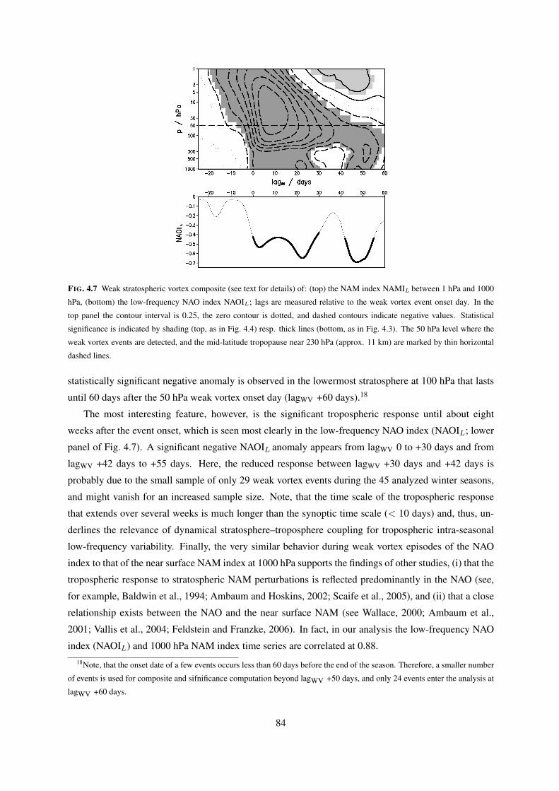
FIG. 4.7 Weak stratospheric vortex composite (see text for details) of: (top) the NAM index NAMIL between 1 hPa and 1000

hPa, (bottom) the low-frequency NAO index NAOIL; lags are measured relative to the weak vortex event onset day. In the

top panel the contour interval is 0.25, the zero contour is dotted, and dashed contours indicate negative values. Statistical

significance is indicated by shading (top, as in Fig. 4.4) resp. thick lines (bottom, as in Fig. 4.3). The 50 hPa level where the

weak vortex events are detected, and the mid-latitude tropopause near 230 hPa (approx. 11 km) are marked by thin horizontal

dashed lines.

statistically significant negative anomaly is observed in the lowermost stratosphere at 100 hPa that lasts

until 60 days after the 50 hPa weak vortex onset day (lagWV +60 days).18

The most interesting feature, however, is the significant tropospheric response until about eight

weeks after the event onset, which is seen most clearly in the low-frequency NAO index (NAOIL; lower

panel of Fig. 4.7). A significant negative NAOIL anomaly appears from lagWV 0 to +30 days and from

lagWV +42 days to +55 days. Here, the reduced response between lagWV +30 days and +42 days is

probably due to the small sample of only 29 weak vortex events during the 45 analyzed winter seasons,

and might vanish for an increased sample size. Note, that the time scale of the tropospheric response

that extends over several weeks is much longer than the synoptic time scale (< 10 days) and, thus, un-

derlines the relevance of dynamical stratosphere–troposphere coupling for tropospheric intra-seasonal

low-frequency variability. Finally, the very similar behavior during weak vortex episodes of the NAO

index to that of the near surface NAM index at 1000 hPa supports the findings of other studies, (i) that the

tropospheric response to stratospheric NAM perturbations is reflected predominantly in the NAO (see,

for example, Baldwin et al., 1994; Ambaum and Hoskins, 2002; Scaife et al., 2005), and (ii) that a close

relationship exists between the NAO and the near surface NAM (see Wallace, 2000; Ambaum et al.,

2001; Vallis et al., 2004; Feldstein and Franzke, 2006). In fact, in our analysis the low-frequency NAO

index (NAOIL) and 1000 hPa NAM index time series are correlated at 0.88.18Note, that the onset date of a few events occurs less than 60 days before the end of the season. Therefore, a smaller number

of events is used for composite and sifnificance computation beyond lagWV +50 days, and only 24 events enter the analysis at

lagWV +60 days.

84

FIG. 4.8 Weak vortex composite of the difference between the number of AB and CB events NAB − NCB per 21 days (left

axis); the lags refer to the central day of each individual 21 days period. Thick lines indicate statistical significance at the 97.5%

level. The right axis relates the number differences to the average number of AB or CB events per 21 days.

c. Wave breaking during stratospheric weak vortex episodes

Returning now to the relation between North Atlantic wave breaking and stratospheric perturbations,

we analyze their effect on the frequencies of AB and CB events in the troposphere during weak vortex

episodes. Since AB and CB events are found to have an opposite effect on the NAO we compute the

difference between the number of detected AB and CB events NAB −NCB , by counting events during

21 days periods to obtain a smoothed result. Small changes of the averaging period do not substantially

modify the results, though for considerably shorter averaging periods the resulting time series becomes

very noisy. The weak vortex composite of this difference is shown in Fig. 4.8, where lags refer to the

center of each individual 21 days period. On average 1.67 AB and 1.67 CB events are detected per

21 days. Accordingly, the right axis in Fig. 4.8 specifies the relative deviation of NAB − NCB per 21

days from the average, that is, the left axis divided by 1.67. Significances are determined by a blocked

boot-strapping approach. Specifically, the same number of non-overlapping 21 days periods as used for

a given lag is selected randomly from the time series. Repeating this procudure for 10000 times, the

upper and lower 97.5%-quantiles of the NAB −NCB distribution are obtained and used as significance

thresholds.

As can be seen from Fig. 4.8, increasingly more CB than AB events are detected during weak vortex

events following lagWV 0, until a significant negative anomaly appears from lagWV +19 days to +30 days

with up to 55% more CB resp. less AB events. This coincides with the negative NAO response period

from lagWV 0 to +30 days. Subsequently, the difference of AB and CB occurrences rapidly drops to zero

until lagWV +34 days, almost simultanously with a reduction of the NAO response until lagWV +36 days.

These results further confirm the close relation between North Atlantic synoptic scale wave breaking and

the NAO.

Furthermore, although the late NAO response (lagWV +42 days to +55 days) is stronger than that

during the earlier period (lagWV 0 to +30 days), it is not accompanied by any significant signal in wave

85

breaking frequencies. Since, additionally, the negative NAM anomaly in the lower stratosphere is already

largely reduced during the later period the results suggest that during weak vortex episodes North Atlantic

wave breaking characteristics respond primarily to the lower stratospheric NAM, and secondarily to the

NAO in the context of the positive feedback mentioned in section 4.3. This positive feedback may also

explain the gradual increase of CB occurrences compared to that of AB events from lagWV 0 to +30 days.

Finally, significantly more CB than AB events are detected about three weeks prior to weak vortex events

(lagWV -18 days and before). However, it is inconclusive how this is related to the onset of weak vortex

episodes. Though one may speculate about a connection to the result of Quiroz (1986) that tropospheric

blocking episodes (which, in turn, are related to CB events as discussed by Woollings et al., 2008, and

also mentioned in section 4.2a of the present study) occur more frequent prior to stratospheric warmings.

From the above results, it is reasonable to argue (i) that tropospheric baroclinic disturbances are,

to some extent, modulated (in terms of their wave breaking characteristics) by variations of the lower

stratospheric flow conditions, and (ii) that the aggregated effect of these changes to individual synoptic

systems, in turn, projects onto the NAO at the Earth’s surface (as also suggested by Charlton et al.,

2004). At this point, however, it should be pointed out that this does not reduce the potential relevance of

alternative mechanisms for dynamical stratosphere–troposphere coupling, as mentioned in section 4.1,

in particular, since the aforementioned stratosphere–troposphere coupling mechanism has not yet been

thoroughly quantified.

d. Relation between wave breaking and non-annular stratospheric variability

The suggested coupling mechanism, that is, the direct modulation of synoptic systems by lower

stratospheric flow conditions, implies a particular sensitivity of the NAO to variations of the stratospheric

flow above the North Atlantic sector, rather than coherent hemispheric scale variability as described by

the 50 hPa NAM. Furthermore, not every weak vortex event is followed by a response in the troposphere,

as shown, for example, by Baldwin and Dunkerton (2001) for the winter 1998/99. Additionally, weak

vortex events are closely related to sudden stratospheric warmings (as shown in section 4.4c above; see

also Tab. 4.1), and sudden stratospheric warmings exhibit a large variety of lower stratospheric flow

patterns associated with polar vortex diplacements and/or splits (e.g., Matthewman et al., 2008), leading

to either an increased or reduced zonal flow above the North Atlantic storm-track region. Thus, the

specific flow evolution in the lower stratosphere during an individual weak vortex event may control the

strength of the associated NAO response, depending on the flow configuration above the North Atlantic

sector and the subsequent changes to tropospheric wave breaking characteristics.

Accordingly, we finally compute the residual 50 hPa geopotential height anomalies, defined as the

low-frequency 50 hPa geopotential height anomaly fields minus the coherent hemispheric scale variabil-

ity given by the 50 hPa NAM (NAMIL). Then, the connection between tropospheric wave breaking

and the non-hemispheric scale variability in the stratosphere is demonstrated by means of AB- and CB-

composites in Fig. 4.9.

The residual 50 hPa signature during AB events (Fig. 4.9c; averaged from lag -4 days to +5 days,

86

FIG. 4.9 Same as Fig. 4.5, but for anomalies of residual 50 hPa geopotential height (i.e., geopotential height minus NAM

variability, see text for details), and the contour interval is 5 gpm; averaged over the period lag -14. . . -5 days (a, b) and lag

-4. . . +5 days (c, d).

w.r.t. wave breaking detection) indicates a cyclonic anomaly near Iceland and, thus, increased westerly

flow above the North Atlantic storm-track at mid-latitudes, while an even stronger anomaly of opposite

sign is observed during CB events (Fig. 4.9d), contributing to anomalous easterly flow above the tropo-

spheric storm-track. Additional inspection of the residual 50 hPa heights up to two weeks prior to CB

events (Fig. 4.9b; averaged from lag -14 days to -5 days) reveals a lower stratospheric evolution that

resembles a polar vortex split and subsequent occurrence of displaced vortex fragments as observed dur-

ing sudden stratospheric warming events. Note, however, that the composite includes all wave breaking

events (e.g., it is not restricted to weak vortex episodes) and, thus, only part of these patterns may in fact

reflect lower stratospheric signatures of sudden stratospheric warmings. On the other hand, before and

during AB events (Fig. 4.9a and c) the residual 50 hPa heights exhibit a tripole pattern with an anticy-

clonic anomaly near the pole and adjacent cyclonic anomalies over the northern North Atlantic and over

Northeast Siberia. This indicates a horizontally stretched vortex, approximately along the 35W–145E

axis, such that lower stratospheric zonal winds are increased above the North Atlantic storm-track region.

Similar wave breaking composites of the residual 50 hPa geopotential height anomalies restricted to

events that occur during weak vortex episodes, however, do not yield statistically significant results due

to the small number of only 29 weak vortex events. Thus, a further extension of a similar analysis will be

done in a future study investigating long-term integrations of a stratosphere resolving general circulation

87

model.

4.5 Discussion and conclusions

This observational study investigates the impact of North Atlantic synoptic scale wave breaking on

the NAO and its connection with the stratosphere, as derived from the ERA-40 reanalysis. Wave breaking

events are detected from daily maps of isentropic potential vorticity at 320 K, using a kinematic criterion

for classification into anticyclonic (AB) and cyclonic wave breaking (CB). By restricting the analysis

to the North Atlantic sector, a total of 1819 wave breaking events is obtained from 45 extended winter

seasons (Nov-Apr) during the 1957-2002 analysis period. Then, the 30% most distinct AB and CB events

are selected (546 events each) from which a North Atlantic wave breaking climatology is constructed.

First, the relation between North Atlantic synoptic scale wave breaking and the NAO is investigated

by means of a composite analysis (section 4.3). Specifically, wave breaking composites are computed of

the time evolution of the NAO, anomalies of surface pressure and of 300 hPa zonal wind and synoptic

scale momentum fluxes. The main conclusions of this part are:

• Anticyclonic (cyclonic) wave breaking is intimately linked with, and drives/reinforces the positive

(negative) phase of the NAO, as previously suggested by Benedict et al. (2004). The positive

(negative) phase of the NAO, in turn, favours the occurrence of AB (CB) events. Thus, the results

indicate a positive feedback between the two kinds of wave breaking and either phase of the NAO.

• Wave breaking in general without any reference to AB- or CB-like behavior, however, does not

have an effect on the NAO, though it occurs preferably during its positive phase.

• An asymmetry between the different kinds of wave breaking exists in the temporal as well as spatial

component, in the sense that anticyclonic wave breaking induces a shorter and stronger response of

the NAO, compared to a slightly more persistent and weaker response to cyclonic wave breaking;

in agreement with the results of the modeling study in chapter 2, applying the same wave breaking

detection method to integrations of a simplified general circulation model.

• AB (CB) occurrences are associated with northward (southward) synoptic scale momentum fluxes

across 45N. Consistently, the North Atlantic eddy-driven jet is strengthened and shifted poleward

during AB events, while it is weakened during CB. These changes to the jet closely resemble

the NAO related changes of the zonal wind in the North Atlantic sector found by Ambaum et al.

(2001).

• Additionally, North Pacific precursors are found about 10 days prior to North Atlantic wave break-

ing events. Specifically, while a strengthened and eastward extended North Pacific jet is observed

prior to North Atlantic CB events, AB events are preceded by a slight northward shift of the North-

east Pacific jet. Franzke et al. (2008) also find an eastward extended North Pacific jet before the

positive phase of the Pacific North American pattern, together with the occurrence of CB events

over the Northeast Pacific.

88

• North Atlantic AB events are associated with a strengthened subtropical jet over the Asian con-

tinent, while CB events drive a more zonally confined response within the North Atlantic sector.

The different zonal extent of the response to AB and CB is also in agreement with chapter 2.

Regarding the wave breaking detection method it is important to note that, since the concept of anticy-

clonic and cyclonic wave breaking is motivated by highly idealized baroclinic wave life cycle simula-

tions, it will hardly be possible to construct any method that identifies either kind of wave breaking for

certain when applied to real atmospheric data. As it is familiar to any synoptician, daily tropopause charts

exhibit a large variety of different IPV signatures as a result of ubiquitous non-linear interactions of the

baroclinic disturbances with waves of different scales and with the time mean flow, in contrast to the

highly simplified conditions in idealized life cycle simulations. Since real baroclinic waves are typically

observed to grow and propagate on strongly non-zonal and time varying background flows, it is some-

times even impossible to decide subjectively whether a certain feature should be classified as anticyclonic

or cyclonic wave breaking. To this end, we repeat the statement of McIntyre and Palmer (1985) that the

concept of breaking Rossby waves does not refer to any automatically recognizable shape. Thus, it is

reasonable, and probably inevitable, to restrict the analysis of anticyclonic and cyclonic wave breaking

to the most distinct AB and CB events. Additionally, the finding that wave breaking in general without

any reference to AB- or CB-like behavior does not affect the NAO further confirms the plausibility of

the results of the present study.

The second part of this study (section 4.4) focuses on the link between North Atlantic synoptic scale

wave breaking and the variability in the lower stratosphere, together with related variations of the NAO.

Lower stratospheric variability is characterized by (i) the 50 hPa northern annular mode (NAM), and

(ii) the residual, that is, the non-annular variability at 50 hPa. Here, we can draw the following main

conclusions:

• On average the 50 hPa NAM index attains larger values during tropospheric AB events than during

CB (though this difference is only marginally significant). Basically, this result is consistent with

the idealized baroclinic wave life cycle study in chapter 3, where anticyclonic wave breaking is

induced by a strengthened stratospheric polar night jet.

• Stratospheric weak vortex events, closely related to sudden stratospheric warmings, exhibit a

downward propagation signature from upper stratospheric levels near the stratopause down to the

Earth’s surface (similar to the result of Baldwin and Dunkerton, 2001), and are followed by a sta-

tistically significant negative NAO response that lasts for up to 55 days after the weak vortex event

onset.

• During weak vortex episodes increasingly more CB than AB events are observed in the tropo-

sphere concurrently with the negative NAO response, and this (significant) difference is maxi-

mized about four weeks after the weak vortex onset. Closer inspection of this analysis suggests

that tropospheric wave breaking chracteristics during lower stratospheric weak vortex events re-

spond primarily to the lower stratospheric NAM, and secondarily to the NAO. The small number

89

of only 29 weak vortex events detected during the 45 extended winter seasons, however, limits the

interpretation of the above results due to reduced statistical significance.

• Tropospheric wave breaking is also linked to non-annular variations in the lower stratosphere, indi-

cating the preferred occurrence of AB (CB) events below westerly (easterly) flow anomalies con-

fined above the North Atlantic storm-track region. Specifically, the residual 50 hPa geopotential

height anomalies prior to and during AB events characterize a horizontally stretched stratospheric

polar vortex, approximately along the 35W–145E axis, while for CB the evolution is suggestive

of a vortex split signature (as observed during sudden stratospheric warmings) with a specific con-

figuration such that a northern North Atlantic anticyclone leads to anomalous easterly flow above

the North Atlantic storm-track.

Hence, the findings of this study strongly suggest that North Atlantic synoptic scale wave breaking is

one key component for stratosphere–troposphere interactions (as previously suggested by, e.g., Baldwin

and Dunkerton, 1999, 2001; Baldwin et al., 2003; Kushner and Polvani, 2004; Charlton et al., 2004;

Wittman et al., 2004, 2007, and chapter 3 of this thesis), in particular, for the response of the NAO to per-

turbations of the polar vortex, as observed during weak vortex episodes or, similarly, sudden stratospheric

warmings. Furthermore, the results indicate a sensitivity of tropospheric wave breaking to non-annular

variability patterns in the lower stratosphere, which represent distortions of the polar vortex. From this

we may speculate that the specific configuration of the non-annular lower stratospheric flow evolution

during weak vortex episodes controls, to some extent, the strength of the associated NAO response.

To further confirm this idea, however, a larger sample of weak vortex events is needed to obtain

improved statistics. Then additional stratospheric variability modes may be extracted to characterize the

differences between weak vortex episodes with strong and with weak tropospheric (NAO) response. This

prompts us to apply a similar analysis to the output of a stratosphere resolving general circulation model

in a future study. Another important issue in this context will be the exact quantification of this and of

alternative mechanisms for dynamical stratosphere–troposphere coupling to allow for an estimation of its

potential relevance for extended-range intra-seasonal weather forecasts as well as climate change.

90

5 Discussion and conclusions

This thesis is concerned with the role of breaking synoptic scale Rossby waves for the North Atlantic

oscillation (NAO) and its coupling with the stratosphere. The subject is addressed from different ap-

proaches, using both a simplified general circulation model and observational data. Chapter 2 examines

the potential of synoptic scale wave breaking to drive NAO-like circulation dipoles19 in a simplified gen-

eral circulation model, and briefly investigates stratospheric influences on tropospheric wave breaking

statistics. The second model study in chapter 3 investigates the response of idealized baroclinic wave life

cycles to stratospheric flow conditions and its relevance for the NAO. And, in chapter 4, observational

evidence for the suggested stratosphere–wave breaking–NAO connection is presented.

While the conclusions obtained by the individual approaches are provided at the end of the respective

chapters (see sections 2.5, 3.5 and 4.5), the present chapter gives a final discussion in the overall context

of this thesis. First, the particular advantages and limitations of the different approaches are discussed in

section 5.1. Then, the main results are summarized in section 5.2 and used to answer the key questions

posed in chapter 1. Finally, a perspective on future research follows in section 5.3.

5.1 Synopsis

The central concept of this work refers to anticyclonic and cyclonic synoptic scale Rossby wave

breaking. The distinction between these characteristic synoptic evolutions of baroclinic waves during

their barotropic decay stage is motivated by simulations of highly idealized baroclinic wave life cycles,

as presented by, for example, Thorncroft et al. (1993). In this respect, the most explicit investigation

of the two kinds of wave breaking is given by chapter 3, using an initial value approach to simulate

individual baroclinic wave life cycles of a single zonal wavenumber under adiabatic and frictionless

conditions. However, — despite the advantage of this approach by using balanced initial conditions,

to be discussed below — the aforementioned assumptions made for this model study are unrealistic

in the sense that the model does not produce localized baroclinic wave packets as observed in zonally

asymmetric forced-dissipative systems like the real atmosphere. On the other hand, the real atmosphere

includes additional complicating aspects of zonally non-uniform and time varying boundary conditions19The term ’NAO-like circulation dipole’ was motivated at the end of section 1.1b by the concept of meridional circulation

dipoles as illustrated in Vallis et al. (2004).

91

and external forcings. In this context, the forced-dissipative model setup used in chapter 2 closes the gap

between idealized baroclinic wave life cycles (chapter 3) and any observational wave breaking analyses

(chapter 4).

Moreover, the setup in chapter 2 is optimal for testing the wave breaking detection method introduced

in that study. It represents the minimal setup for simulating a large number of anticyclonic and cyclonic

wave breaking events (in the sense of the LC1 and LC2 life cycle paradigms) in a forced-dissipative

system, that is, a baroclinically unstable mid-latitude jet in a primitive equation model with spherical

geometry. Accordingly, this study brings out most clearly the basic features of anticyclonic and cyclonic

wave breaking within localized baroclinic wave packets — and its effect on the large scale extratropical

circulation in the absence of a zonally non-uniform background flow and boundary conditions.

Additionally, the convincing results from the successful application of the wave breaking detection

method to the simplified model atmosphere in chapter 2 increases the confidence in the results of the

observational study in chapter 4, which is restricted to the shorter and more complex reanalysis dataset.

Note, that for idealized baroclinic wave life cycle simulations, on the other hand, such a method is

not needed since either kind of wave breaking can be generated by controling the prescribed initial

conditions.

However, regarding the influence of the stratosphere on tropospheric wave breaking characteristics,

the implications from the forced-dissipative model approach in chapter 2 are limited. Though in that

study a sensitivity of tropospheric wave breaking statistics to the strength of the stratospheric polar

night jet is obtained, and this sensitivity is induced by a purely stratospheric perturbation, this does not

necessarily imply the existence of a direct stratosphere–wave breaking connection. Alternatively, a zonal

mean secondary circulation response to changed stratospheric wave drag may induce changes in the

mean tropospheric flow which in turn affects tropospheric wave breaking characteristics (see Kushner

and Polvani, 2004, for a detailed discussion of this issue; see also section 2.4e of this thesis). Here,

the advantage of the initial value approach in the baroclinic wave life cycle study (chapter 3) becomes

apparent. By using balanced initial zonal flow conditions (with zero meridional and vertical velocity),

the obtained changes in life cycle bahavior can be fully attributed to a direct response of the baroclinic

waves to stratospheric flow conditions, since the initial zonal mean secondary circulation is zero and thus

identical among the different simulations.

Finally, the observational approach in chapter 4 provides evidence that the suggested stratosphere–

wave breaking–NAO connection is relevant to the real atmosphere. The main limitations of that study are

due the short observational data record, in particular, with respect to the response of tropospheric wave

breaking to stratospheric perturbations related to major sudden stratospheric warmings, since on average

only one such event is observed per 1.5 years. On the other hand, it is important to note that none of the

modeling studies includes an NAO-like variability mode in the sense of a zonally localized meridional

circulation dipole at some preferred longitude. Hence, the observational study in chapter 4 represents an

important contribution since it is the only part that explicitly refers to the effect of synoptic scale wave

breaking on the large scale flow in a zonally confined region, i.e., on the North Atlantic oscillation.

92

5.2 Discussion and answers to key questions

In this section the main results of this thesis are summarized and discussed in the context of the

key questions posed in chapter 1. In the following the key questions are repeated, together with the

corresponding answers:

Q-1 Does synoptic scale anticyclonic (cyclonic) wave breaking drive meridional circulation dipoles

resembling the positive (negative) phase of the NAO?

• Synoptic scale anticyclonic and cyclonic wave breaking does, in fact, drive meridional circu-

lation dipoles that resemble the positive and negative phase of the NAO, respectively. How-

ever, a distinct asymmetry is found between the two kinds of wave breaking. The full asym-

metry is obtained by the forced-dissipative model approach in chapter 2, which allows to

view the evolution in the context of the entire baroclinic wave packet:

• Anticyclonic wave breaking (AB) takes place at the center of an eastward and equatorward

propagating wave group as it grows in amplitude and reaches the equatorward side of the

jet. Due to downstream development a major AB event is typically preceded by a weaker

precursory AB event in the upstream wave (see Fig. 2.7). From the interaction of these two

AB events a strong and short-lived positive phase NAO-like dipole emerges at the surface,

but not at upper tropospheric levels where a more complex tripole pattern is produced.

• Cyclonic wave breaking (CB) takes place at the center of an eastward propagating wave

group within a zonal wave guide, and is triggered preferably on the poleward flank of the jet

as the center of the wave group reaches the diffluent flow field to the west of a preexisting

blocking (or negative NAO-like) pattern (see Fig. 2.7). From this single CB event a strong

and more persistent negative phase NAO-like dipole emerges at upper levels, but not at the

surface where a weaker and NE-SW oriented dipole is generated.

• Moreover, the CB response dipole pattern is shifted northward against the AB response pat-

tern in both, the forced-dissipative model study (chapter 2) and in the idealized baroclinic

wave life cycle study (chapter 3), whereas the observational results in chapter 4 exhibit an

opposite shift. It is speculated that this difference results from an additional response of the

quasi-stationary waves which are not included in the model studies.

Q-2 Does stronger (weaker) westerly flow in the lower stratosphere induce anticyclonic (cyclonic) wave

breaking in the troposphere?

• Stronger westerly flow in the lower stratosphere does, in fact, favour anticyclonic wave break-

ing during the decay stage of tropospheric baroclinic waves, while cyclonic wave breaking is

favoured by weaker stratospheric flow.

• From the baroclinic wave life cycle study in chapter 3 it is suggested that the interaction

between the baroclinic wave and the lower stratospheric zonal flow is essentially non-linear,

93

since stratosphere induced changes during the linear stage do only partially explain the ob-

tained response. The details of the interaction mechanism, however, are not yet understood.

• The baroclinic response to stratospheric flow conditions is limited to a small parameter

regime close to the transition point from AB- to CB-like behavior, with respect to the merid-

ional profile of the basic state (or initial) zonal flow. However, the frequent occurrence of

both, AB- and CB-like behavior in the real atmosphere within the North Atlantic storm-track

region suggests that this sensitive parameter regime is just most relevant to baroclinic proce-

ses in the North Atlantic sector.

• In the observational study (chapter 4) it is shown explicitly how synoptic scale wave break-

ing in the North Atlantic sector is particularly sensitive to lower stratospheric flow conditions

above the zonally localized strom-track region, rather than to hemispheric scale flow varia-

tions. This suggests that wave breaking characteristics in the North Atlantic sector do not

depend simply on the strength of the northern annular mode (NAM), but also on the synoptic

evolution related to non-annular variability in the lower stratosphere. This is of particular

interest in the context of sudden stratospheric warmings which, to a first approximation, re-

flect negative NAM anomalies, but are also associated with large case to case variability in

terms of the non-annular flow evolution in the lower stratosphere due to strong distortions of

the polar vortex. Hence, the specific flow configuration above the North Atlantic storm-track

region during sudden stratospheric warming events may control the strength of the associated

tropospheric response in the NAO.

Q-3 What explicit observational evidence does exist for the suggested stratosphere–wave breaking–

NAO connection?

• By applying the wave breaking detection method, which is introduced in chapter 2, to the

ERA-40 reanalysis explicit observational evidence is presented (in chapter 4) that anticy-

clonic wave breaking in the North Atlantic sector drives the positive phase of the NAO, and

that cyclonic wave breaking drives the negative phase. This differs from the approach of

Benedict et al. (2004) where this relation is suggested implicitly by a composite analysis

based on the NAO.

• Furthermore, during persistent negative NAM episodes in the lower stratosphere, signifi-

cantly more CB than AB events are observed, concurrently with a negative response of the

NAO. However, the causal relationship between wave breaking, the lower stratosphere and

the NAO cannot be identified for certain from this approach, although the composite analysis

in section 4.4c indeed suggests a direct response of tropospheric wave breaking characteris-

tics to lower stratospheric flow conditions. Nevertheless, it should be noted that this aspect

is affected by the relatively short data record that enters the analysis and, thus, statistical

confidence is limited.

94

Hence, this work provides considerable evidence for dynamical stratosphere–troposphere coupling

by tropospheric synoptic scale systems. In particular, the importance of anticyclonic and cyclonic syn-

optic scale Rossby wave breaking for the NAO and its coupling with the stratosphere — as suggested by

the literature (see chapter 1 and the introductions to the chapters 2 to 4) — has been demonstrated, from

a modeling as well as observational approach.

5.3 Perspective

Finally, this section presents a perspective on future research issues, which may serve as a reasonable

extension to the investigations of this thesis. As mentioned in chapter 4, the observational analysis of the

relation between synoptic scale wave breaking and the lower stratospheric flow, also considering non-

annular variability (section 4.5), should be complemented by a corresponding study with a sophisticated

general circulation model (GCM) that includes both, a well resolved stratosphere and a realistic repre-

sentation of the NAO. Then, the results obtained from chapter 4 are to be verified and, subsequently, the

analysis can be extended to much longer time series to overcome the main drawback of the observational

study, namely, the small number of large stratospheric perturbations. In particular, the relevance of non-

annular variability during sudden stratospheric warmings for controlling the strength of the associated

response in the NAO (see chapter 4) is of great interest in this context. Additionally, such GCM experi-

ments would allow to investigate whether a relation exists between synoptic scale wave breaking in the

eastern North Atlantic and the circumglobal wave guide teleconnection pattern, which originates in the

western part of the Asian subtropical jet (Branstator, 2002, see section 4.3b), with possible implications

for hemispheric scale impacts of North Atlantic wave breaking dynamics.

Furthermore, an extension of the forced-dissipative model approach in chapter 2 to a zonally non-

uniform model setup will be useful to gain further insight into (i) the interaction between baroclinic

wave packets and the flow in the lower stratosphere, and (ii) the role of quasi-stationary planetary waves

for the localization of synoptic scale wave breaking in zonally confined storm-tracks, as observed, for

example, in the North Atlantic sector (Martius et al., 2007). In particular, as shown by Gerber and Polvani

(2008), this kind of simplified GCM setup produces plausible stratosphere–troposphere interactions in

terms of downward propagating NAM anomalies. Since (i) from that and other studies (see chapter 1) it

is suggested that stratosphere–troposphere coupling by synoptic scale systems is particularly important

with respect to negative NAM anomalies in the lowermost stratosphere (which persist for up to two

months after the perturbation onset; for observational evidence, see Baldwin and Dunkerton, 2001, and

chapter 4 of this thesis) and (ii) since the lack of statistical confidence in the observational analysis in

chapter 4 relating tropospheric wave breaking characteristics to negative stratospheric NAM anomalies

is largest during the late stage of such perturbations (see section 4.4), very long-term integrations of

simplified GCMs will be optimal to study this statistically weak but important link.

The probably most important issue, however, will be the identification of the non-linear interaction

mechanism that induces the transition in baroclinic wave life cycle behavior found in chapter 3 — that

95

is, the understanding of the basic dynamic processes involved in this aspect of stratosphere–troposphere

coupling. This will require an approach that makes use of a hierarchy of models for the simulation of

baroclinic wave life cycles, also including even simpler models than the spherical geometry primitive

equation model employed in chapter 3. On the other hand, models of higher complexity like the sim-

plified GCM used in chapter 2 may help to investigate the dependence of the interaction mechanism

on tropospheric flow conditions, particularly in a statistical sense. More specifically, if the interac-

tion mechanism only applies under certain tropospheric flow conditions related to hardly predictable

high-frequency variability, then the potential of the stratosphere to improve tropospheric extended-range

weather forecasts might be significantly reduced.

96

Acknowledgments

The successful completion of this thesis, and the research it is based on, is owed to a large extent to

the support and encouragement of many individuals, and would have been impossible without them. In

the following I want to acknowledge the most important contributions to this work.

First of all, I am indebted to my supervisor Prof. Klaus Fraedrich for giving me the opportunity

to start this challenging project in the Theoretische Meteorologie group at the Universitat Hamburg,

for his ambition to ensure the continued progress of my work and, in particular, for allowing me the

maximum scope for my scientific orientation. I am also grateful for many stimulating discussions with

Frank Lunkeit and his constructive criticism that helped to focus on the relevant aspects. On the technical

side I want to express my gratitude to Edilbert Kirk and Frank Sielmann for the excellent administration

and maintanance of the IT-system and their prompt response to all my detailed questions in this context.

Furthermore, I thank Martin Keller for sharing with me his enthusiasm for numerous issues in large

scale atmospheric dynamics, and Christian Franzke and Richard Greatbatch for their encouragement and

interest in my research — Helga Behr for lively communication about the actual synoptic situation, and

also my colleagues Simon Blessing, Gregor Knorr, Guido Schroder and Frank Sienz for semi-scientific

activities inside and outside the university, and all my other colleagues who contributed in various ways

to my success. Last but not least, special thanks go to the people outside the university for keeping me

in touch with real life over the past years and, thus, contributed indirectly to more efficient work.

This work was funded by the Deutsche Forschungsgemeinschaft, Sonderforschungsbereich 512 “Cy-

clones and the North Atlantic climate system”. The Model & Data group at the Max Planck Institute for

Meteorology is acknowledged for providing the ERA-40 reanalysis dataset.

97

98

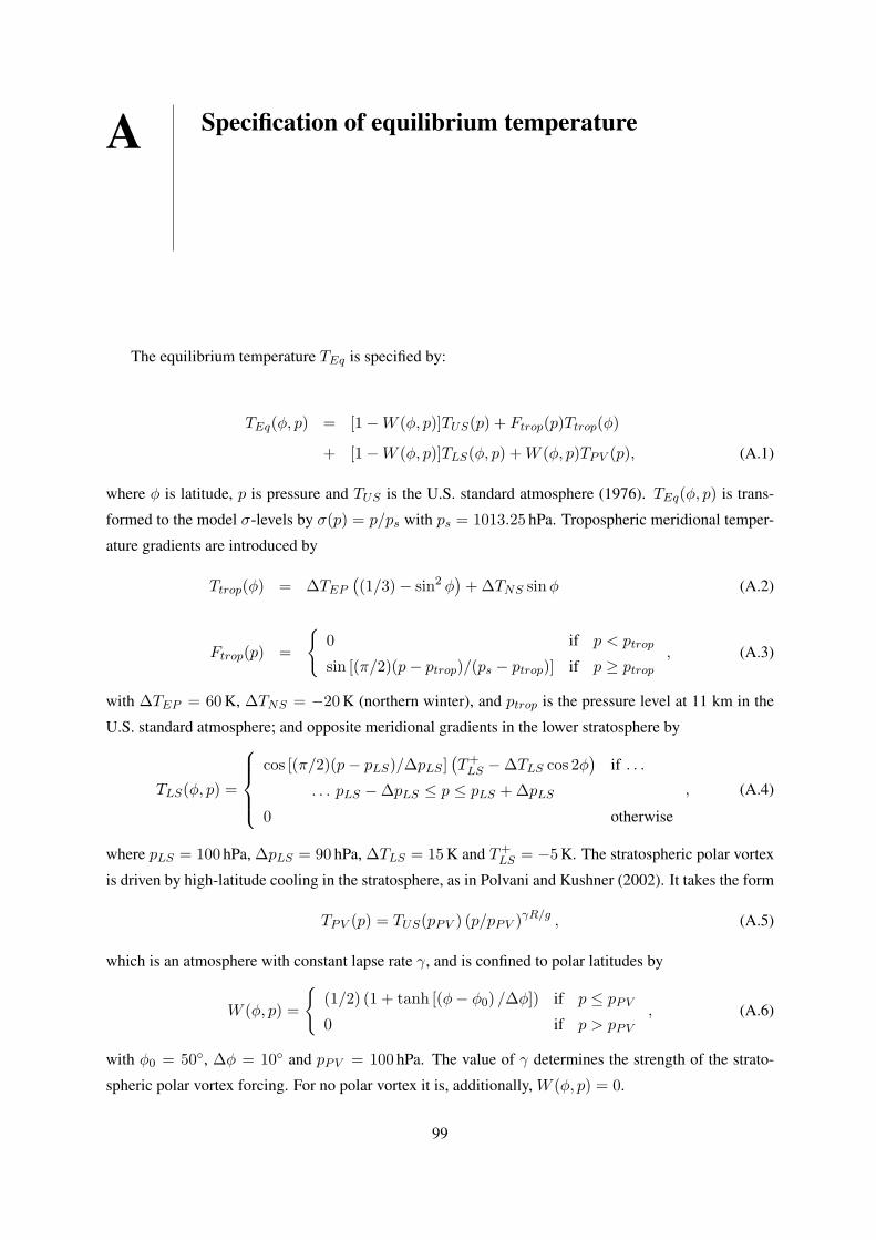
A Specification of equilibrium temperature

The equilibrium temperature TEq is specified by:

TEq(φ, p) = [1−W (φ, p)]TUS(p) + Ftrop(p)Ttrop(φ)

+ [1−W (φ, p)]TLS(φ, p) + W (φ, p)TPV (p), (A.1)

where φ is latitude, p is pressure and TUS is the U.S. standard atmosphere (1976). TEq(φ, p) is trans-

formed to the model σ-levels by σ(p) = p/ps with ps = 1013.25 hPa. Tropospheric meridional temper-

ature gradients are introduced by

Ttrop(φ) = ∆TEP

((1/3)− sin2 φ

)+ ∆TNS sinφ (A.2)

Ftrop(p) =

0 if p < ptrop

sin [(π/2)(p− ptrop)/(ps − ptrop)] if p ≥ ptrop

, (A.3)

with ∆TEP = 60 K, ∆TNS = −20 K (northern winter), and ptrop is the pressure level at 11 km in the

U.S. standard atmosphere; and opposite meridional gradients in the lower stratosphere by

TLS(φ, p) =

cos [(π/2)(p− pLS)/∆pLS ]

(T+

LS −∆TLS cos 2φ)

if . . .

. . . pLS −∆pLS ≤ p ≤ pLS + ∆pLS

0 otherwise

, (A.4)

where pLS = 100 hPa, ∆pLS = 90 hPa, ∆TLS = 15 K and T+LS = −5 K. The stratospheric polar vortex

is driven by high-latitude cooling in the stratosphere, as in Polvani and Kushner (2002). It takes the form

TPV (p) = TUS(pPV ) (p/pPV )γR/g , (A.5)

which is an atmosphere with constant lapse rate γ, and is confined to polar latitudes by

W (φ, p) =

(1/2) (1 + tanh [(φ− φ0) /∆φ]) if p ≤ pPV

0 if p > pPV

, (A.6)

with φ0 = 50, ∆φ = 10 and pPV = 100 hPa. The value of γ determines the strength of the strato-

spheric polar vortex forcing. For no polar vortex it is, additionally, W (φ, p) = 0.

99

100

B Setup of balanced initial zonal flow

The balancing procedure of obtaining the mass field that balances the prescribed initial zonal flow

(3.1) essentially follows Hoskins and Simmons (1975); see their appendix. The model solves the non-

dimensional primitive equations in σ-coordinates for the prognostic variables: absolute vorticity ζ =

ζΩ−1, divergence D = DΩ−1, temperature T = Ta−2Ω−2R (R is the gas constant of dry air) and

the logarithm of surface pressure ln p? = ln(p?p−10 ). By imposing the restrictions of zero meridional

and vertical velocity and zero zonal variation and time tendencies on the model equations, the balance

equation is obtained:

− ∂

∂µ

(ζU)−∇2

(U2

2(1− µ2)

)︸ ︷︷ ︸

F

=∂

∂µ

((1− µ2)T

∂ ln p?

∂µ

)︸ ︷︷ ︸

M1

+∇2Φ︸︷︷︸M2

, (B.1)

where µ = sin φ, ∇2 = ∂/∂µ[(1 − µ2)∂/∂µ], Φ = Φa−2Ω−2 is the non-dimensional geopotential and

U = ua−1Ω−1(1− µ2)1/2 (so that ζ = 2µ− ∂U/∂µ). From (B.1) Φ is given by

∇−2 (F −M1)︸ ︷︷ ︸Y

= Φ. (B.2)

The hydrostatic equation T = −∂Φ/∂ lnσ may be expressed in the integrated and discretized form

as Φn = gTn, where Φn and Tn are column vectors specifying the values of Φ resp. T at each full-level,

n indicates the horizontal spectral mode (n = 1, . . . , 21 represents the zonally uniform modes which are

symmetric about the equator, and n = 0 the horizontal mean), and the matrix g is defined by gij = ∆ ln σ

for i < j, gii = 1− [σj−0.5∆ lnσ/∆σ] for i = j and gij = 0 for i > j, with ∆σ = σj+0.5 − σj−0.5 and

∆ lnσ = ln σj+0.5 − lnσj−0.5.20 Using the same notation for Y , (B.2) yields

g−1Yn = Tn. (B.3)

In cases of zero initial zonal flow (3.1) at z = 0 (shear parameter UCS = 0), it is required that

∂ ln p?/∂µ = 0. Hence, Y is independent of ln p? and T can readily be obtained from (B.3). In all other

cases (shear parameter UCS 6= 0) it is required that ∂ ln p?/∂µ 6= 0 and, for a given surface pressure

20Note, that the matrix g differs from that in Hoskins and Simmons (1975).

101

field, T is determined iteratively from (B.3), using the start values Tn>0 = 0 and setting T0 to the U.S.

Standard Atmosphere (1976). Convergence is reached after less than ten iterations.

A first guess surface pressure field is obtained by numerical integration of the geostrophic wind

relation at σ = 1

∂ ln p?

∂µ= − µ

1− µ2

(2U

T ?+

11− µ2

U2

T ?

), (B.4)

where U is approximated by u|z=0 a−1Ω−1(1 − µ2)1/2 from (3.1), and the surface temperature T ? by

numerical integration of the thermal wind relation (written in z) at z = 0

∂T ?

∂µ= −2H

µ

1− µ2

(∂U

∂z+

11− µ2

U∂U

∂z

), (B.5)

where U is approximated as in (B.4) and ∂U/∂z by (∂u/∂z)|z=0 a−1Ω−1(1 − µ2)1/2. The surface

pressure field is then optimized to reduce large vertical two grid oscillations by minimization of the

cost function f = (∑21

n=1(A>Tn)2)1/2, where A> = (1,−1, 1, . . .). Optimization of only four surface

pressure modes (n = 1, . . . , 4) is found to be sufficient to obtain smooth temperature fields, after less

than 200 iterations of a downhill simplex method.

102

C Northern annular mode time series

FIG. C.1 Low-frequency (periods > 10 days) northern annular mode (NAM) index time series during the 45 extended winter

seasons (November- April) from 1957/58 to 2001/02, as derived from the 23 pressure levels (1 hPa to 1000 hPa) of the ERA-40

reanalysis. The index time series of each level is normalized to have zero mean and unit standard deviation. Contour interval

is 0.5, the zero contour is omitted; blue (red) shading indicates positive (negative) values that exceed ±0.5 standard deviations.

The horizontal dashed line at 230 hPa marks the mid-latitude tropopause near 11 km. For details on the computation of the

NAM index time series see section 4.2b. The onset days of persistent weak stratospheric vortex episodes at 50 hPa, as defined

in section 4.4b (see also Tab. 4.1), are marked by green squares.

103

FIG. C.1 continued.

104

FIG. C.1 continued.

105

106

References

Abatzoglou, J. T. and G. Magnusdottir, 2006: Opposing effects of reflective and nonreflective planetary

wave breaking on the NAO. J. Atmos. Sci.

Ambaum, M. H. P. and B. J. Hoskins, 2002: The NAO troposphere-stratosphere connection. J. Climate,

15, 1969–1978.

Ambaum, M. H. P., B. J. Hoskins, and D. B. Stephenson, 2001: Arctic oscillation or North Atlantic

oscillation. J. Climate, 14, 3495–3507.

Andrews, D. G., J. R. Holton, and C. B. Leovy, 1987: Middle atmosphere dynamics. Academic Press,

489 pp.

Appenzeller, C. and H. C. Davies, 1992: Structure of stratospheric intrusions into the troposphere. Na-

ture, 358, 570–572.

Balasubramanian, G. and S. T. Garner, 1997: The role of momentum fluxes in shaping the life cycle of a

baroclinic wave. J. Atmos. Sci., 54, 510–533.

Baldwin, M. P., X. Cheng, and T. J. Dunkerton, 1994: Observed correlations between winter-mean

tropospheric and stratospheric circulation anomalies. Geophys. Res. Lett., 21, 1141–1144.

Baldwin, M. P., M. Dameris, and T. G. Shepherd, 2007: How will the stratosphere affect climate change?

Science, 316, 1576–1577.

Baldwin, M. P. and T. J. Dunkerton, 1999: Propagation of the Arctic oscillation from the stratosphere to

the troposphere. J. Geophys. Res.

———, 2001: Stratospheric harbingers of anomalous weather regimes. Science, 294, 581–584.

Baldwin, M. P., D. B. Stephenson, D. W. J. Thompson, T. J. Dunkerton, A. J. Charlton, and A. O’Neill,

2003: Stratospheric memory and skill of extended-range weather forecasts. Science, 301, 636–640.

Benedict, J. J., S. Lee, and S. B. Feldstein, 2004: Synoptic view of the North Atlantic oscillation. J.

Atmos. Sci., 61, 121–144.

Blackmon, M. L., 1976: A climatological spectral study of the 500mb geopotential height of the northern

hemisphere. J. Atmos. Sci., 33, 1607–1623.

Blessing, S., K. Fraedrich, M. Junge, T. Kunz, and F. Lunkeit, 2005: Daily North-Atlantic oscillation

(NAO) index: statistics and its stratospheric polar vortex dependence. Meteorol. Z., 14, 763–769.

107

Branstator, G., 2002: Circumglobal teleconnections, the jet stream wave guide, and North Atlantic oscil-

lation. J. Climate, 15, 1893–1910.

Canziani, P. O. and W. E. Legnani, 2003: Tropospheric–stratospheric coupling: Extratropical synoptic

systems in the lower stratosphere. Quart. J. Roy. Meteor. Soc., 129, 2315–2329.

Chang, E. K. M., S. Lee, and K. L. Swanson, 2002: Storm track dynamics. J. Climate, 15, 2163–2183.

Charlton, A. J., A. O’Neill, W. A. Lahoz, and A. C. Massacand, 2004: Sensitivity of tropospheric fore-

casts to stratospheric initial conditions. Quart. J. Roy. Meteor. Soc., 130, 1771–1792.

Charlton, A. J. and L. M. Polvani, 2007: A new look at stratospheric sudden warmings. Part I: Climatol-

ogy and modeling benchmarks. J. Climate, 20, 449–469.

Charney, J. G. and P. G. Drazin, 1961: Propagation of planetary-scale disturbances from the lower into

the upper atmosphere. J. Geophys. Res., 66, 83–109.

Drevillon, M., L. Terray, P. Rogel, and C. Cassou, 2001: Mid-latitude Atlantic SST influence on Euro-

pean winter climate variability in the NCEP reanalysis. Clim. Dyn., 18, 331–344.

Duchon, C. E., 1979: Lanczos filtering in one and two dimensions. J. Appl. Meteor., 18, 1016–1022.

Esler, J. G. and P. H. Haynes, 1999: Baroclinic wave breaking and the internal variability of the tropo-

spheric circulation. J. Atmos. Sci., 56, 4014–4031.

Feldstein, S. B., 2000: The timescale, power spectra, and climate noise properties of teleconnection

patterns. J. Climate, 13, 4430–4440.

———, 2003: The dynamics of NAO teleconnection pattern growth and decay. Quart. J. Roy. Meteor.

Soc., 129, 901–924.

Feldstein, S. B. and C. Franzke, 2006: Are the North Atlantic oscillation and the northern annular mode

distinguishable? J. Atmos. Sci., 63, 2915–2930.

Fraedrich, K., 1994: An ENSO impact on Europe? A review. Tellus, 46A, 541–552.

Fraedrich, K., C. Bantzer, and U. Burkhardt, 1993: Winter climate anomalies in Europe and their asso-

ciated circulation at 500 hPa. Clim. Dyn., 8, 161–175.

Fraedrich, K., E. Kirk, U. Luksch, and F. Lunkeit, 2005: The portable university model of the atmosphere

(PUMA): Storm track dynamics and low-frequency variability. Meteorol. Zeitschrift, 14, 735–745.

Fraedrich, K., E. Kirk, and F. Lunkeit, 1998: Portable University Model of the Atmosphere. Tech.

Rep. 16, DKRZ.

Franzke, C., S. B. Feldstein, and S. Lee, 2008: Synoptic analysis of the Pacific-North American telecon-

nection pattern. J. Atmos. Sci., submitted.

108

Franzke, C., S. Lee, and S. B. Feldstein, 2004: Is the North Atlantic oscillation a breaking wave? J.

Atmos. Sci., 61, 145–160.

Frisius, T., F. Lunkeit, K. Fraedrich, and I. A. James, 1998: Storm-track organization and variability in

a simplified atmospheric global circulation model (SGCM). Quart. J. Roy. Meteor. Soc., 124, 1019–

1043.

Fritts, D. C. and M. J. Alexander, 2003: Gravity wave dynamics and effects in the middle atmosphere.

Rev. Geophys., 41, 1003, doi:10.1029/2001RG000 106.

Gerber, E. P. and L. M. Polvani, 2008: Stratosphere–troposphere coupling in a relatively simple AGCM:

The importance of stratospheric variability. J. Climate, submitted.

Gerber, E. P., S. Voronin, and L. M. Polvani, 2007: Testing the annular mode autocorrelation timescale

in simple atmospheric general circulation models. Mon. Weath. Rev., accepted.

Haines, K. and J. C. Marshall, 1987: Eddy-forced coherent structures as a prototype of atmospheric

blocking. Quart. J. Roy. Meteor. Soc., 113, 681–704.

Hartmann, D. L., 2000: The key role of lower-level meridional shear in baroclinic wave life cycles. J.

Atmos. Sci., 57, 389–401.

Hartmann, D. L. and F. Lo, 1998: Wave-driven zonal flow vacillation in the southern hemisphere. J.

Atmos. Sci., 1303–1315.

Hartmann, D. L. and P. Zuercher, 1998: Response of baroclinic life cycles to barotropic shear. J. Atmos.

Sci., 55, 297–313.

Haynes, P. H., C. J. Marks, M. E. McIntyre, T. G. Shepherd, and K. P. Shine, 1991: On the downward

control of extratropical diabatic circulations by eddy-induced mean zonal forces. J. Atmos. Sci., 48,

651–678.

Held, I. M. and M. J. Suarez, 1994: A proposal for the intercomparison of the dynamical cores of

atmospheric general circulation models. Bull. Amer. Meteor. Soc., 75, 1825–1830.

Hoskins, B. J., M. E. McIntyre, and A. W. Robertson, 1985: On the use and significance of isentropic

potential vorticity maps. Quart. J. Roy. Meteor. Soc., 111, 877–946.

Hoskins, B. J. and A. J. Simmons, 1975: A multi-layer spectral model and the semi-implicit method.

Quart. J. Roy. Meteor. Soc., 101, 637–655.

Hurrell, J. W., 1995: Decadal trends in the North Atlantic oscillation: Regional temperatures and precip-

itation. Science, 269, 676–679.

109

Hurrell, J. W., Y. Kushnir, G. Ottersen, and M. Visbeck, (Eds.) , 2003: The North Atlantic oscillation:

Climate significance and environmental impact. Geophys. Monogr., Vol. 134. Amer. Geophys. Union,

279 pp.

Illary, L., 1984: A diagnostic study of the potential vorticity in a warm blocking anticyclone. J. Atmos.

Sci., 41, 3518–3526.

Juckes, M. N. and M. E. McIntyre, 1987: A high-resolution one-layer model of breaking planetary waves

in the stratosphere. Nature, 328, 590–596.

Kushner, P. J. and L. M. Polvani, 2004: Stratosphere-troposphere coupling in a relatively simple AGCM:

The role of eddies. J. Climate, 17, 629–639.

Labitzke, K. and H. van Loon, 1988: Associations between the 11-year solar cycle, the QBO and the

atmosphere. Part I: The troposphere and stratosphere in the northern hemisphere in winter. J. Atmos.

Terr. Phys., 50, 197–206.

Lorenz, D. J. and D. L. Hartmann, 2001: Eddy–zonal flow feedback in the southern hemisphere. J.

Atmos. Sci., 58, 3312–3327.

———, 2003: Eddy–zonal flow feedback in the northern hemisphere winter. J. Climate, 16, 1212–1227.

Luo, D., 2005: A barotropic envelope Rossby soliton model for block-eddy interaction. Part I: Effect of

topography. J. Atmos. Sci., 62, 5–21.

Magnusdottir, G. and P. H. Haynes, 1996: Wave activity diagnostics applied to baroclinic wave life

cycles. J. Atmos. Sci., 53, 2317–2353.

Martius, O., C. Schwierz, and H. C. Davies, 2007: Breaking waves at the tropopause in the wintertime

northern hemisphere: Climatological analyses of the orientation and the theoretical LC1/2 classifica-

tion. J. Atmos. Sci., 64, 2576–2592.

Matsuno, T., 1970: Vertical propagation of stationary planetary waves in the winter northern hemisphere.

J. Atmos. Sci., 27, 871–883.

———, 1971: A dynamical model of the stratospheric sudden warming. J. Atmos. Sci., 28, 1479–1494.

Matthewman, N. J., J. G. Esler, A. J. Charlton-Perez, and L. M. Polvani, 2008: A new look at strato-

spheric sudden warmings. Part III: Polar vortex evolution and vertical structure. J. Climate, submitted.

McIntyre, M. E. and T. N. Palmer, 1983: Breaking planetary waves in the stratosphere. Nature, 305,

593–600.

———, 1985: A note on the general concept of wave breaking for Rossby and gravity waves. Pure Appl.

Geophys., 123, 964–975.

110

Nakamura, M. and R. A. Plumb, 1994: The effects of flow asymmetry on the direction of Rossby wave

breaking. J. Atmos. Sci., 51, 2031–2045.

Orlanski, I., 2003: Bifurcation of eddy life cycles: Implications for storm track variability. J. Atmos. Sci.,

60, 993–1023.

Pelly, J. L. and B. J. Hoskins, 2003: A new perspective on blocking. J. Atmos. Sci., 60, 743–755.

Perlwitz, J. and H.-F. Graf, 1995: The statistical connection between tropospheric and stratospheric

circulation of the northern hemisphere in winter. J. Climate, 8, 2281–2295.

———, 2001: Troposphere–stratosphere dynamic coupling under strong and weak polar vortex condi-

tions. Geophys. Res. Lett., 28, 271–274.

Perlwitz, J. and N. Harnik, 2003: Observational evidence of a stratospheric influence on the troposphere

by planetary wave reflection. J. Climate, 16, 3011–3026.

Peters, D. and D. W. Waugh, 1996: Influence of barotropic shear on the poleward advection of upper-

tropospheric air. J. Atmos. Sci., 53, 3013–3031.

Polvani, L. M. and P. J. Kushner, 2002: Tropospheric response to stratospheric perturbations in a rela-

tively simple general circulation model. Geophys. Res. Lett., 29, 1114, doi:10.1029/2001GL014 284.

Polvani, L. M. and R. Saravanan, 2000: The three-dimensional structure of breaking Rossby waves in

the polar wintertime stratosphere. J. Atmos. Sci., 57, 3663–3685.

Quiroz, R. S., 1986: The association of stratospheric warmings with tropospheric blockings. J. Geophys.

Res., 91, 5277–5285.

Riviere, G. and I. Orlanski, 2007: Characteristics of the Atlantic storm-track activity and its relation with

the North Atlantic oscillation. J. Atmos. Sci.

Rossby, C.-G., 1939: Relation between variations in the intensity of the zonal circulation of the atmo-

sphere and the displacements of the semi-permanent centers of action. J. Marine Res., 2, 38–55.

Scaife, A. A., J. R. Knight, G. K. Vallis, and C. K. Folland, 2005: A stratospheric influ-

ence on the winter NAO and North Atlantic surface climate. Geophys. Res. Lett., 32, L18 715,

doi:10.1029/2005GL023 226.

Scinocca, J. F. and P. H. Haynes, 1998: Dynamical forcing of stratospheric planetary waves by tropo-

spheric baroclinic eddies. J. Atmos. Sci., 55, 2361–2392.

Scott, R. K., D. G. Dritschel, L. M. Polvani, and D. W. Waugh, 2004: Enhancement of Rossby wave

breaking by steep potential vorticity gradients in the wintertime stratosphere. J. Atmos. Sci., 61, 904–

918.

111

Shabbar, A., J. Huang, and K. Higuchi, 2001: The relation between the wintertime North Atlantic oscil-

lation and blocking episodes in the North Atlantic. Int. J. Climatol., 21, 355–369.

Shutts, G. J., 1983: The propagation of eddies in diffluent jetstreams: eddy vorticity forcing of ’blocking’

flow fields. Quart. J. Roy. Meteor. Soc., 109, 737–761.

Simmons, A. J. and D. Burridge, 1981: An energy and angular-momentum conserving vertical finite-

difference scheme and hybrid vertical coordinates. Mon. Wea. Rev., 109, 758–766.

Simmons, A. J. and B. J. Hoskins, 1980: Barotropic influences on the growth and decay of nonlinear

baroclinic waves. J. Atmos. Sci., 37, 1679–1684.

Snyder, C., W. C. Skamarock, and R. Rotunno, 1991: A comparison of primitive-equation and semi-

geostrophic simulations of baroclinic waves. J. Atmos. Sci., 48, 2179–2194.

Thompson, D. W. J., M. P. Baldwin, and J. M. Wallace, 2002: Stratospheric connection to northern

hemisphere wintertime weather: Implications for prediction. J. Climate, 15, 1421–1428.

Thompson, D. W. J., J. C. Furtado, and T. G. Shepherd, 2006: On the tropospheric response to anomalous

stratospheric wave drag and radiative heating. J. Atmos. Sci., 63, 2616–2629.

Thompson, D. W. J. and J. M. Wallace, 1998: The Arctic oscillation signature in the wintertime geopo-

tential height and temperature fields. Geophys. Res. Lett., 25, 1297–1300.

Thorncroft, C. D. and B. J. Hoskins, 1990: Frontal cyclogenesis. J. Atmos. Sci., 47, 2317–2336.

Thorncroft, C. D., B. J. Hoskins, and M. E. McIntyre, 1993: Two paradigms of baroclinic-wave life-cycle

behaviour. Quart. J. Roy. Meteor. Soc., 119, 17–55.

Ulbrich, U. and P. Speth, 1991: The global energy cycle of stationary and transient atmospheric waves -

results from ECMWF analyses. Meteorol. Atmos. Phys., 45, 125–138.

U.S. Standard Atmosphere, 1976: U.S. Government Printing Office, Washington, D.C.

Vallis, G. K., E. P. Gerber, P. J. Kushner, and B. A. Cash, 2004: A mechanism and simple dynamical

model of the North Atlantic oscillation and annular modes. J. Atmos. Sci., 264–280.

Walker, G. T. and E. W. Bliss, 1932: World Weather V. Mem. Roy. Meteor. Soc., 4, 53–84.

Wallace, J. M., 2000: North Atlantic oscillation/annular mode: Two paradigms-one phenomenon. Quart.

J. Roy. Meteor. Soc.

Wallace, J. M. and D. S. Gutzler, 1981: Teleconnections in the geopotential height fields during the

northern hemisphere winter. Mon. Wea. Rev., 109, 784–812.

112

Waugh, D. W., R. A. Plumb, R. J. Atkinson, M. R. Schoeberl, L. R. Lait, P. A. Newman, M. Loewenstein,

C. R. Webster, and R. D. May, 1994: Transport of material out of the stratospheric Arctic vortex

through Rossby wave breaking. J. Geophys. Res., 99, 1071–1088.

Whitaker, J. S. and C. Snyder, 1993: The effects of spherical geometry on the evolution of baroclinic

waves. J. Atmos. Sci., 50, 597–612.

Wittman, M. A. H., A. J. Charlton, and L. M. Polvani, 2007: The effect of lower stratospheric shear on

baroclinic instability. J. Atmos. Sci., 64, 479–496.

Wittman, M. A. H., L. M. Polvani, R. K. Scott, and A. J. Charlton, 2004: Stratospheric influence on

baroclinic lifecycles and its connection to the Arctic oscillation. Geophys. Res. Lett., 31, L16 113,

doi:10.1029/2004GL020 503.

Woollings, T., B. J. Hoskins, M. Blackburn, and P. Berrisford, 2008: A new Rossby wave-breaking

interpretation of the North Atlantic oscillation. J. Atmos. Sci., 65, 609–626.

Yu, J.-Y. and D. L. Hartmann, 1993: Zonal flow vacillation and eddy forcing in a simple GCM of the

atmosphere. J. Atmos. Sci., 50, 3244–3259.

113