The robustness of parametric statistical methods - Pabst · The robustness of parametric statistical methods 177 Experimenters know that they nearly never really meet observations

Psychology Science, Volume 46, 2004 (2), p. 175-208

The robustness of parametric statistical methods

DIETER RASCH1, VOLKER GUIARD

2

1. Abstract

In psychological research sometimes non-parametric procedures are in use in cases, where the corresponding parametric procedure is preferable. This is mainly due to the fact that we pay too much attention to the possible violation of the normality assumption which is needed to derive the exact distribution of the statistic used in the parametric approach.

An example is the t-test and its non-parametric counterpart, the Wilcoxon (Mann-Whitney) test. The Wilcoxon test compares the two distributions and may lead to signifi-cance even if the means are equal due to the fact that higher moments in the two populations differ. On the other hand the t-test is so robust against non-normality that there is nearly no need to use the Wilcoxon test. In this paper results of a systematic research of the robustness of statistical procedures against non-normality are presented. These results have been ob-tained in a research group in Dummerstorf (near Rostock) some years ago and have not been published systematically until now. Most of the results are based on extensive simulation ex-periments with 10 000 runs each. But there are also some exact mathematically derived results for very extreme deviations from normality (two- and three-point distributions). Generally the results are such that in most practical cases the parametric approach for inferences about means is so robust that it can be recommended in nearly all applications.

Key words: definition of robustness, simulation studies, robustness of interal estimations,

robustness of statistical tests, robustness against deviations from the normal distribution

1 Dieter Rasch, BioMath – Institute of Applied Mathematical Statistics in Biology and Medicine Ltd.,

Rostock; E-mail: [email protected] 2 Volker Guiard, Research Institute for the Biology of Farm Animals, Dummerstorf, Research Unit Genetics

& Biometry

D. Rasch, V. Guiard 176

2. Definition of Robustness against Non-Normality In Herrendörfer, G. (ed.) (1980) and Bock (1982) several robustness concepts like those

of Box and Tiao (1964), Huber (1964) and Zielinsky (1977) have been discussed. The con-cept of ε–robustness was introduced which was used in the robustness research presented in this paper. This concept is here introduced for the construction of confidence intervals in a simplified way.

Definition 1 Let ad 3 be a confidence estimation based on an experimental design Vn of size n con-

cerning a parameter θ of a class G of distributions with (nominal) confidence coefficient 1 - α (0<α<1) in G. For an element h ∈ H ⊃ G of a class H of distributions which contains G we denote by 1–α( Vn, h) the actual confidence coefficient of dα . Then we call dα ε–robust in H if α and α( Vn, h) deviate from each other by less than ε for any element in H (some-times we also say by less than 100ε% and than speak about 100ε% - robustness).

If we are only interested in not too large α( Vn, h)-values (conservative procedures are not considered as non-robust), we call dα ε*–robust in H if α( Vn, h) does not exceed α by more than ε*.

In an analogue way the ε– and ε*–robustness of tests or selection procedures can be de-fined. Due to the fact that a test for testing a null hypothesis 0 0:H θ θ= can be performed by accepting 0H if θ0 is inside the confidence interval and reject it otherwise, definition 1 includes the robustness of a test concerning the significance level.

In this paper we use for G the family of univariate normal 2( ( , ) )N µ σ − distributions and for H the Fleishman system of distributions and/or truncated normal distributions.

Definition 2 A distribution belongs to the Fleishman system (Fleishman, 1978) if its first four mo-

ments exist and if it is the distribution of the transform

2 3y a bx cx d x= + + + (1)

where x is a standard normal random variable (with mean 0 and variance 1).

By a proper choice of the coefficients a, b, c and d the random variable y will have any quadruple of first four moments 2

1 2( , , , )µ σ γ γ . By 1γ and 2γ we denote the skewness (standardized third moment) and the kurtosis (standardized fourth moment) of any distribu-tion, respectively. For instance any normal distribution (ie. any element of G) with mean µ and variance σ2 can be represented as a member of the Fleishman system by choosing a = µ, b = σ and c = d = 0. This shows that we really have H ⊃ G as demanded in definition 1.

3 Random variables are underlined.

The robustness of parametric statistical methods 177

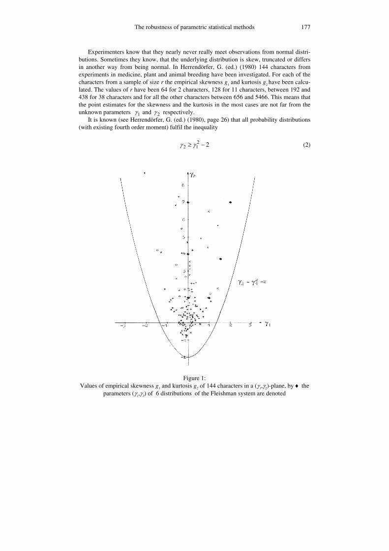
Experimenters know that they nearly never really meet observations from normal distri-butions. Sometimes they know, that the underlying distribution is skew, truncated or differs in another way from being normal. In Herrendörfer, G. (ed.) (1980) 144 characters from experiments in medicine, plant and animal breeding have been investigated. For each of the characters from a sample of size r the empirical skewness g1 and kurtosis g2 have been calcu-lated. The values of r have been 64 for 2 characters, 128 for 11 characters, between 192 and 438 for 38 characters and for all the other characters between 656 and 5466. This means that the point estimates for the skewness and the kurtosis in the most cases are not far from the unknown parameters 1γ and 2γ respectively.

It is known (see Herrendörfer, G. (ed.) (1980), page 26) that all probability distributions (with existing fourth order moment) fulfil the inequality

22 1 2γ γ≥ − (2)

Figure 1:

Values of empirical skewness g1 and kurtosis g2 of 144 characters in a (γ1,γ2)-plane, by ♦ the parameters (γ1,γ2) of 6 distributions of the Fleishman system are denoted


Empirical distributions fulfils an analogue equation in the estimated skewness g1 and kurtosis g2 respectively

22 1 2g g≥ − (3)

The equality sign in (2) or (3) defines a parabola in the 1 2( , )γ γ – plane { 1 2( , )g g –

plane}. In Figure 1 the position of the 1 2( , )g g –values calculated for the 144 characters in that

parabola are shown. Therefore we selected seven 1 2( , )γ γ –values in that parabola for the robustness investi-

gations reported in this paper. The values together with the coefficient a, b, c and d of the elements in the Fleishman system for the case µ = 0 (what means a = - c) and σ = 1 (what means b2 + 6bd + 2c2 + 15d2 = 1) are given in Table 1. They are marked in Figure 1 by a♦.

Table 1:

1 2( , )γ γ –values and the corresponding coefficients in (2)

No of dis-tribution 1γ 2γ c = -a b d

1 0 0 0 1 0 2 0 1.5 0 0.866993269415 0.042522484238 3 0 3.75 0 0.748020807992 0.077872716101 4 0 7 0 0.630446727840 0.110696742040 5 1 1.5 0.163194276264 0.953076897706 0.006597369744 6 1.5 3.75 0.221027621012 0.865882603523 0.027220699158 7 2 7 0.260022598940 0.761585274860 0.053072273491

The values of b, c and d in Table 1 are taken from Table A3 in Nürnberg (1982), some of

them can be found already in Fleishman (1972).

1. Simulation Experiments in Robustness Research In the simulation experiments (as also in the statistical analysis of experimental results)

we mainly use linear statistical models with an error term. We investigate the behaviour of statistical procedures like confidence estimation, hypotheses testing and selection procedures which have been derived (and thus are exact) under the assumption of normal error terms. The question is: „What happens with the properties of these procedures if we replace the normal error by an error term following a Fleishman (or a truncated normal) distribution with non-zero 1γ and 2γ ?“

There are only very few analytical results to answer this question for sample sizes 2 and 3 which are useless for practical purposes. For very extreme (two- and three-point distribu-tions) exact answers have been given by Herrendörfer (1980) and Herrendörfer and Rasch (1981). The results in our paper are based on simulation experiments.


By simulation we mean that we use random numbers to simulate the observations of an artificial experiment for a given underlying model. In the one-sample case we denote the size of the artificial experiment by n.

We use the following example to demonstrate the basic ideas.

Example 1 A sample ( that is a vector of identically and independently distributed (abbr. i.i.d.) ran-

dom variables) of size n is drawn from a 2( , )N µ σ - distribution. A (realized) confidence

interval is calculated from the realization of the random sample (the observations) if σ - as usually - is unknown by:

[ ( 1;1 ) ; ( 1;1 ) ]2 2

s sy t n y t nn n

α α− − − + − − (4)

where the sample mean y is the point estimate of µ , the sample standard deviation s is the

point estimate of σ and ( 1;1 )2

t n α− − is the (1 )

2α

− quantile of the central t-distribution

with n – 1 d.f.. The corresponding random interval (with random bounds as functions of the

sample) covers the unknown µ with probability (1 )2a

− as long as the sample really stems

from a normal distribution. Amongst all intervals with such a property the interval (4) is optimal what means it has the smallest expected width. Non-parametric intervals have a larger expected width if the normal assumption is true. In this case the linear model for the n elements

iy of the random sample has the simple form

, 1,...,= + =i iy µ e i n (5)

The experimental design Vn in (5) is simply given by the sample size n (there is no struc-

ture in the experiment). The robustness against truncation (occurring in any selecting process like in schools or in agricultural artificial selection) of normal distributions of this confi-dence estimation (and the corresponding test) is investigated in simulation experiment 1 below.

We use besides the t-quantiles other abbreviations (for quantiles) as given in the follow-ing Table.


Table 2: Abbreviations used in this paper

Term Abbreviation Degrees of freedom d.f. Identically and independently distributed i.i.d. P-quantile (percentile) of the N(0;1)distribution u(P) P-quantile (percentile) of the t-distribution with f d.f. t(f; P) P-quantile (percentile) of the F-distribution with 1f and 2f d.f. respectively 1 2( , ; )F f f P

P-quantile (percentile) of the 2χ -distribution with f d.f. CQ(f; P)

3.1 Pseudo-Random Number Generators Because we cannot generate random numbers by means of a computer program, in

simulation experiments so-called pseudo-random numbers (PRN) are used. In Herrendörfer, G. (ed.) (1980) and by FEIGE et al. (1985) 18 generators of PRN uniformely distributed in (0, 1) have been tested against several properties which may negatively influence the simula-tion results (like periodicity or correlation).

Finally we used a generator which was developed by Teuscher (1979) according to an idea of Mac Laren and Marsaglia (1965). This generator is a combination of the following two generators:

1012 mod1049339k kx x −= (6)

and

28

1 08323 mod 2 , 1i iy y y−= =

Within the initialisation phase the values 1 128,...,x x will be generated. In order to calcu-

late the random values , 1...,iZ i = we calculate the index I with 1 128I≤ ≤ , being the

integer part of 211 / 2iy+ . Then we select Ix from the x-values above and calculate

/1049339i IZ x= . Within the vector 1 128( ,..., )x x the value Ix will be substituted by the

next value of the kx -values, i.e. 128 ix + .

The Z-values generated from (6) are PRN uniformly distributed in the interval (0,1). They have to be transformed into PRN with a standard normal distribution and then by (1) in PRN of the Fleishman system. FEIGE et al. (1985) tested 5 different transformations of the Z- values into standard normal PRN u and proposed the following for further use. At first we define for 0.5Z <

2lnz Z= − and c = 1


and for 0.5Z ≥

( )2ln 1z Z= − − and c = -1

Then with coefficients given by Odeh and Evans (1974) (see also Feige et al., 1985, page

31) calculate

[( ){ }( ){ } ]4 3 2 1 0

4 3 2 1 0

p z p z p z p z pu c z

q z q z q z q z q

⋅ + + + + = ⋅ + ⋅ + + + +

.

These N(0;1)-PRN have been used directly (after truncation) in simulation experiment 1

and have been transformed by (1) into Fleishman variates for the other experiments.

3.2 Planning the Size and the Scope of the Simulation Experiments A simulation experiment has to be planned in the same way as experiments in psychol-

ogy (see Rasch, 2003) or other fields. The aim of the simulation experiments discussed in this paper is to evaluate probabilities as the significance level of a test or the confidence coefficient of an interval estimation or the probability of a correct selection in selection procedures. More specifically we are interested to find out, whether under non-normality the nominal probability differs by more than an ε from the actual value. We restrict ourselves in the present paper on a significance level of α = 0.05, a confidence coefficient 1-α =0.95 and a probability of a correct selection β = 0.05. For ε* in definition 1 we choose 20% of α and this is 0.01. That means on the basis of the simulation of N samples of size n each we will test the pair of hypotheses (for selection problems α must be replaced by β) :

0 : 0.05: 0.05A

HH

αα

=

>

(if α is smaller than 0.05 we do not exceed the nominal significance level).

To determine the number of simulated samples we proceed like an experimenter in life science planning a real life experiment. We follow the principle explained in paragraph 4.4 in Rasch (2003) and fix the significance level of this test at α*=0.01 and the value of the power function at α + d = 0.05 + 0.006 = 0.056 at 0.85. To determine the number of simu-lated samples we edit the constants above into the CADEMO module MEANS, branch „Comparing a probability with a constant” and receive the result 9894. Therefore 10 000 runs were used in each of the simulation experiments below.

3.3 The Layout of the Simulation Experiments for several problems We report simulation experiments for the investigation of the robustness of tests, confi-

dence estimation and selection procedures. Each of the statistical inference methods was


perfomed 10 000 times for each case included in the research program. Then the number R of negative results has been observed and used to calculate the observed error rate by α as an estimate of the actual risk α . The distributions to be simulated are special cases of the Fleishman system given in Table 1. In paragraph 4 we report only the results for the nominal risk α = 0.05 but in Herrendörfer, G. (ed.) (1980), Guiard, V. (ed.) (1981), Rasch, D. and G. Herrendörfer (ed.) (1982), Rasch, D. (ed.) (1985), Rudolph, P.E. (ed.) (1985 a), and Guiard, V. and Rasch, D. (ed.) (1987) results for α = 0.01 and α = 0.1 are also given. The normal distri-bution was included on one hand to check the correctness of the programs. On the other hand – like in the investigation of asymptotic tests – the results for the normal have been of inter-est too.

We demonstrate this in the following example which is also used to show how more complicated cases than that in example 1 can be handled.

Example 2 Let us consider the non-linear regression model with unknown parameters α, β and γ.

= + +ixi iy e eγα β 1,..., )i n= (7)

with i.i.d. random errors ie . Here Vn is given not only by the sample size n but by the alloca-tion of the n x-values. We define a design with k different x-values kxxx ,...,, 21 which occur with the frequencies knnn ,...,, 21 , respectively, by

=≥= ∑

=

nnknx

nx

nx

Vk

jj

k

kn

12

2

1

1 ,3,......

(8)

The distribution of the least squares estimators of the three parameters is unknown for fi-

nite samples even if the error terms are normally distributed. What is known is the asymp-totic distribution on which statistical tests can be based (see RASCH, 1995).

Let us now describe the simulation experiments whose results will be reported in para-graph 4. The first 6 experiments deal with tests for means and variances. But the results are also useful for the construction of confidence intervals. Between a confidence interval with coefficient 1-α and a test with a significance level α a one-to-one correspondence exists. As long as the hypothesis value µ0 lies inside the interval, H0 is accepted and rejected otherwise. On the other hand, all accepted µ0 – values are inside the interval and all rejected outside. We report the tests here because they give additional information about the power (or the risk of the second kind).


Simulation Experiment 1 – One-sample tests for the mean This experiment has been planned and performed by TEUSCHER (1985).

In this experiment three tests have been compared to test the hypothesis H0 : µ = µ0 against:

a) 0:AH µ µ+ > ,

b) 0:AH µ µ− < and

c) 0:AH µ µ≠ .

with a sample of size n.

If the variance 2σ of the assumed normal distribution is known, the u-test was used as follows:

Test 1 Calculate 0y -

u z nµ

σ= = and reject H0 :

a) if u > u(1-α), b) if u < - u(1-α),

c) if 12

> −

u u α.

For unknown 2σ two tests have been investigated:

Test 2 The one-sample t-test: Calculate 0y

t = s

nµ−

and reject H0 : a) if t > t(n-1;1-α), b) if t <- t(n-1;1-α),

c) if 1;12

> − −

t t n α.

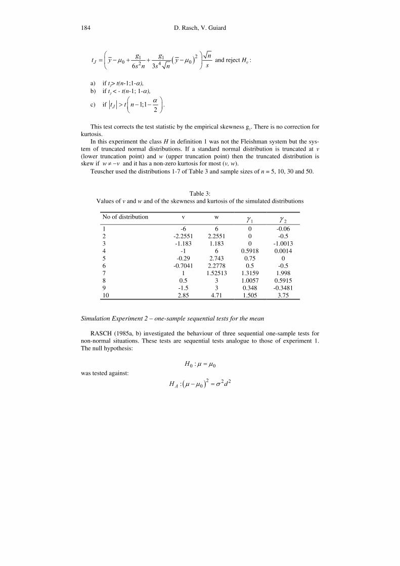
Test 3 The modified Johnson-test based on JOHNSON N, J. (1978) Calculate with an estimate g1 of the skewness γ1:


( )21 10 02 46 3

Jg g nt y y

ss n s nµ µ

= − + + −

and reject H0 :

a) if tJ> t(n-1;1-α), b) if tJ < - t(n-1; 1-α),

c) if 1;12

> − −

Jt t n α.

This test corrects the test statistic by the empirical skewness g1. There is no correction for

kurtosis. In this experiment the class H in definition 1 was not the Fleishman system but the sys-

tem of truncated normal distributions. If a standard normal distribution is truncated at v (lower truncation point) and w (upper truncation point) then the truncated distribution is skew if w v≠ − and it has a non-zero kurtosis for most (v, w).

Teuscher used the distributions 1-7 of Table 3 and sample sizes of n = 5, 10, 30 and 50.

Table 3: Values of v and w and of the skewness and kurtosis of the simulated distributions

No of distribution v w

1γ 2γ

1 -6 6 0 -0.06 2 -2.2551 2.2551 0 -0.5 3 -1.183 1.183 0 -1.0013 4 -1 6 0.5918 0.0014 5 -0.29 2.743 0.75 0 6 -0.7041 2.2778 0.5 -0.5 7 1 1.52513 1.3159 1.998 8 0.5 3 1.0057 0.5915 9 -1.5 3 0.348 -0.3481 10 2.85 4.71 1.505 3.75

Simulation Experiment 2 – one-sample sequential tests for the mean RASCH (1985a, b) investigated the behaviour of three sequential one-sample tests for

non-normal situations. These tests are sequential tests analogue to those of experiment 1. The null hypothesis:

0 0:H µ µ=

was tested against:

( )2 2 20:AH dµ µ σ− =


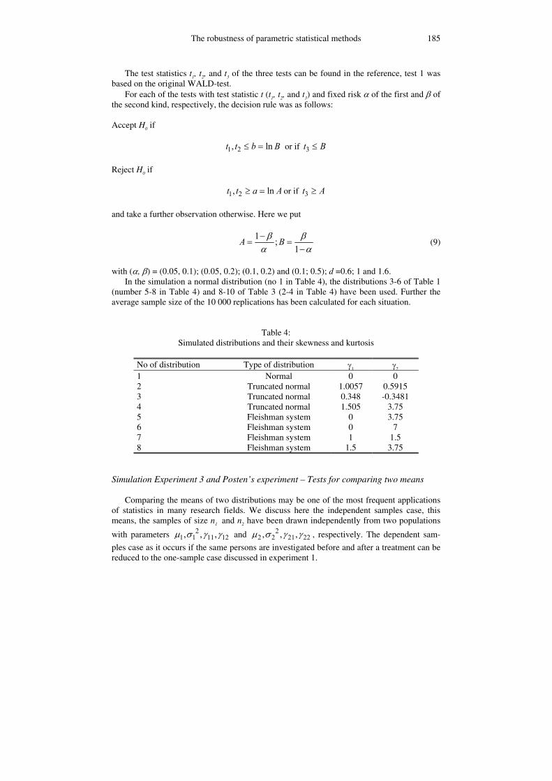
The test statistics t1, t2, and t3 of the three tests can be found in the reference, test 1 was based on the original WALD-test.

For each of the tests with test statistic t (t1, t2, and t3) and fixed risk α of the first and β of the second kind, respectively, the decision rule was as follows:

Accept H0 if

1 2, lnt t b B≤ = or if 3t B≤

Reject H0 if

1 2, lnt t a A≥ = or if 3t A≥

and take a further observation otherwise. Here we put

1 ;

1A Bβ β

α α−

= =−

(9)

with (α, β) = (0.05, 0.1); (0.05, 0.2); (0.1, 0.2) and (0.1; 0.5); d =0.6; 1 and 1.6.

In the simulation a normal distribution (no 1 in Table 4), the distributions 3-6 of Table 1 (number 5-8 in Table 4) and 8-10 of Table 3 (2-4 in Table 4) have been used. Further the average sample size of the 10 000 replications has been calculated for each situation.

Table 4: Simulated distributions and their skewness and kurtosis

No of distribution Type of distribution γ1 γ2

1 Normal 0 0 2 Truncated normal 1.0057 0.5915 3 Truncated normal 0.348 -0.3481 4 Truncated normal 1.505 3.75 5 Fleishman system 0 3.75 6 Fleishman system 0 7 7 Fleishman system 1 1.5 8 Fleishman system 1.5 3.75

Simulation Experiment 3 and Posten’s experiment – Tests for comparing two means Comparing the means of two distributions may be one of the most frequent applications

of statistics in many research fields. We discuss here the independent samples case, this means, the samples of size n1 and n2 have been drawn independently from two populations

with parameters 21 1 11 12, , ,µ σ γ γ and 2

2 2 21 22, , ,µ σ γ γ , respectively. The dependent sam-

ples case as it occurs if the same persons are investigated before and after a treatment can be reduced to the one-sample case discussed in experiment 1.


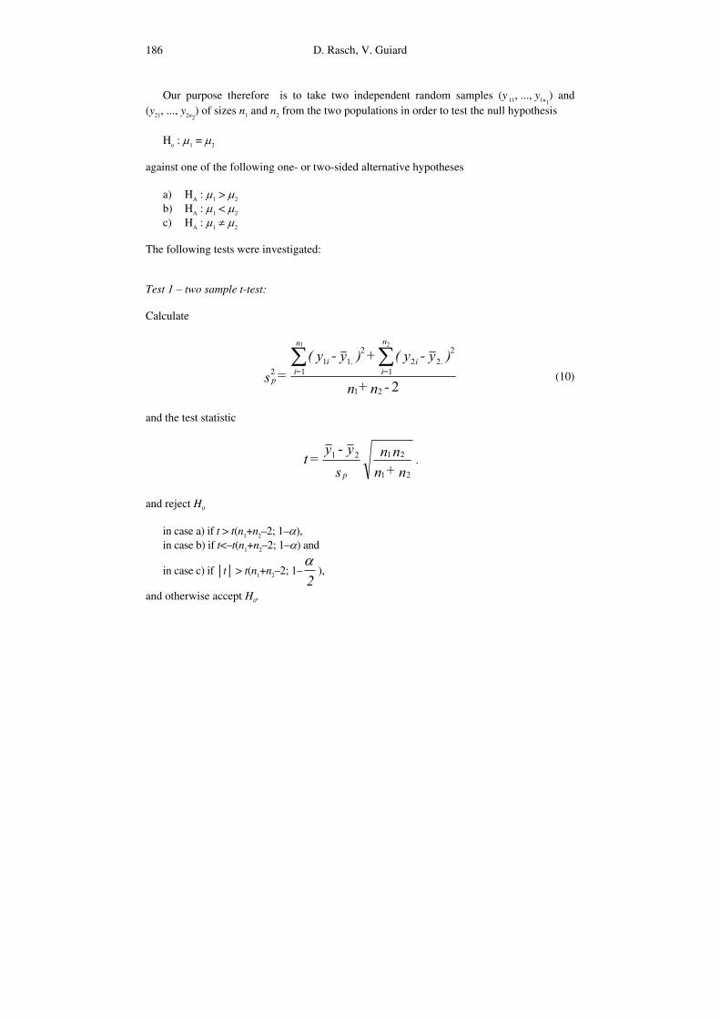
Our purpose therefore is to take two independent random samples (y 11, ..., y1n1) and

(y21, ..., y2n2) of sizes n1 and n2 from the two populations in order to test the null hypothesis

Ho : µ1 = µ2

against one of the following one- or two-sided alternative hypotheses a) HA : µ1 > µ2 b) HA : µ1 < µ2 c) HA : µ1 ≠ µ2

The following tests were investigated:

Test 1 – two sample t-test:

Calculate

221

2.22

1

2.11

12

21

-n+n

)y-y( + )y-y( = s

i

n

=ii

n

=ip

∑∑ (10)

and the test statistic

n+nnn

sy-y

= tp 21

2121 .

and reject H0

in case a) if t > t(n1+n2–2; 1–α), in case b) if t<–t(n1+n2–2; 1–α) and

in case c) if │t│ > t(n1+n2–2; 1–2α

),

and otherwise accept H0.


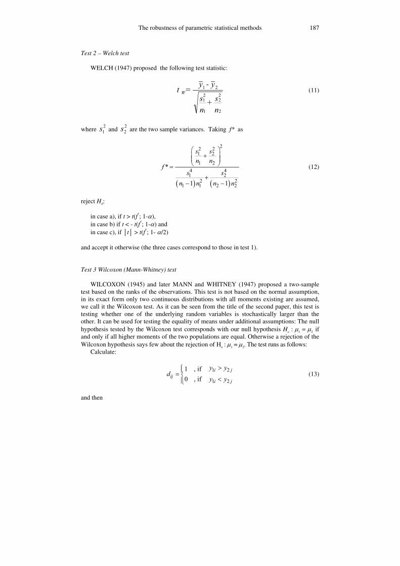
Test 2 – Welch test WELCH (1947) proposed the following test statistic:

ns +

ns

y - y = t W

2

22

1

21

21 (11)

where 21s and

22s are the two sample variances. Taking f* as

( ) ( )

22 21 2

1 24 41 2

2 21 1 2 2

*

1 1

s sn n

fs s

n n n n

+

=

+− −

(12)

reject H0:

in case a), if t > t(f*; 1-α), in case b) if t < - t(f*; 1-α) and in case c), if │t│ > t(f*; 1- α/2)

and accept it otherwise (the three cases correspond to those in test 1).

Test 3 Wilcoxon (Mann-Whitney) test WILCOXON (1945) and later MANN and WHITNEY (1947) proposed a two-sample

test based on the ranks of the observations. This test is not based on the normal assumption, in its exact form only two continuous distributions with all moments existing are assumed, we call it the Wilcoxon test. As it can be seen from the title of the second paper, this test is testing whether one of the underlying random variables is stochastically larger than the other. It can be used for testing the equality of means under additional assumptions: The null hypothesis tested by the Wilcoxon test corresponds with our null hypothesis Ho : µ1 = µ2 if and only if all higher moments of the two populations are equal. Otherwise a rejection of the Wilcoxon hypothesis says few about the rejection of Ho : µ1 = µ2. The test runs as follows:

Calculate:

1 2

1 2

1 , if0 , if

i jij

i j

y yd

y y

>= < (13)

and then


( ) 1 21 1

121 1

12 = =

+= = + ∑∑

n n

iji j

n nW W d . (14)

Reject Ho

in case a), if W > ( )1 2, ;1W n n α−

in case b) if W < ( )1 2, ;W n n α and

in case c), if either W < 1 2, ;2

W n n α

or W > 1 2, ;12

W n n α −

and accept it otherwise (the three cases correspond to those in test 1). Extensive tables of the quantiles ( )1 2, ;W n n α are given by VERDOOREN (1963).

Test 4 – Range test of Lord

LORD (1947) proposed the following test for small samples: Calculate the ranges (maximum minus minimum sample value) w1 and w2 of the two

samples and then

21

21

wwyyTLord +

−=

and reject Ho

in case a), if LordT > ( )1 2, ;1n nτ α−

in case b) if LordT < ( )1 2, ;n nτ α , and

in case c), if either LordT < 1 2, ;2

n n ατ

or LordT > 1 2, ;12

n n ατ −

and accept it otherwise (the three cases correspond to those in test 1). Tables of the quantiles

( )1 2, ;n n Pτ are given in Lord’s paper.

The following tests are due to TIKU (1980).

Test 5 Tiku’s T-test A modified maximum likelihood test for censored samples described in TUCH-

SCHERER (1985, page 161 as test T12).


Test 6 Tiku’s Tc-test A Welch type modification of test 5 described in TUCHSCHERER (1985, page 161 as

test T13). The situation of experiment 3 concerning test 1 and test 3 was one of the few studies al-

ready investigated with a sufficient large number of runs before our robustness research started. These simulations were done by Posten (1985) using 40 000 runs for test 3 and 100 000 runs for test 1.

Posten used the union of Pearson system distributions with the normal distributions as the class H of distributions in definition 1. He simulated distributions in the Pearson system in a grid of (γ1 , γ2) – values with γ1 = 0(0.4)2 and γ2 = -1.6(0.4)4.8 and sample sizes of 5(5)30 equal in both samples.

Posten stated in his 1985 paper: „It would seem, therefore, that further studies of the effects of variance heterogeneity on

the two tests would be needed over an extensive practical family of non-normal distributions before a single procedure might be specified as a somewhat general choice for the two-sample location problem”

This was the reason that Tuchscherer started a further experiment (Tuchscherer 1985, Tuchscherer and Pierer 1985).

The authors of the second paper used the 7 Fleishman distributions of Table 1, first kind risks of 0.01; 0.05 and 0.1; the tests 1-6 and 7 further tests and a ratio of the two variances of 0.5; 1; and 1.5 and a sample size of 5 in population 1 and of 5 and 10 in population 2.

In Guiard and Rasch (ed.) (1987) for the tests 1 – 4 further results can be found for trun-cated normal distributions with (γ1 , γ2) – values: (1.0057; 0.5915); (0.348; -0.3488) and (1.505; 3.75).

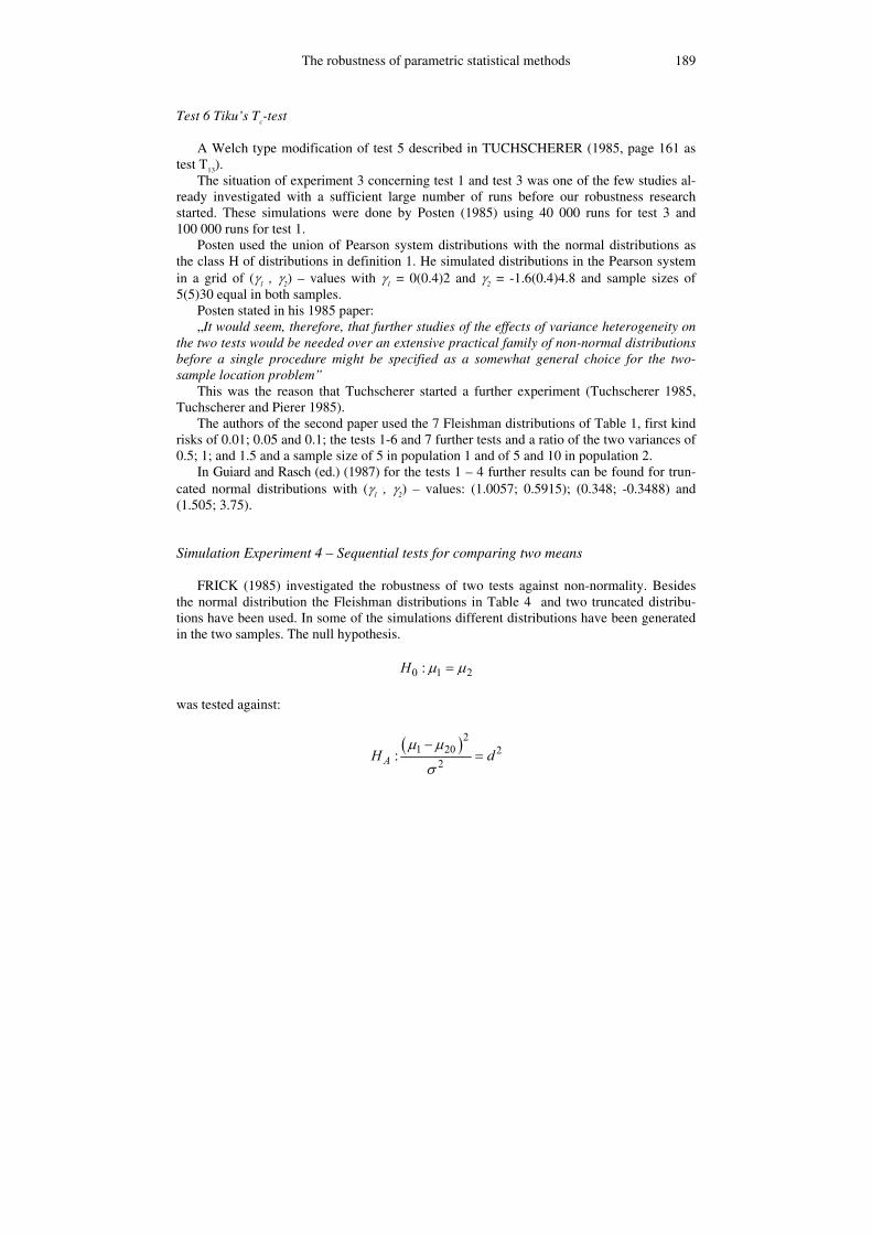
Simulation Experiment 4 – Sequential tests for comparing two means FRICK (1985) investigated the robustness of two tests against non-normality. Besides

the normal distribution the Fleishman distributions in Table 4 and two truncated distribu-tions have been used. In some of the simulations different distributions have been generated in the two samples. The null hypothesis.

0 1 2:H µ µ=

was tested against:

( )21 20 2

2:AH dµ µ

σ

−=


Test 1 – Hajnal’s test HAJNAL (1961) proposed the following procedure: Calculate

( )2 2 2

21 1exp , ,

2 2 2 2

d f d tQ HK K f t

− + = +

with

21 2

1 2

1 1 , 2,= + = + −K f n nn n

1 2

P

y yt

s K−

=⋅

,

2ps from (10) and the confluent hyper-geometric function H.

With A and B as in experiment 2, we accept H0 if Q<B and reject it, if Q>A. Otherwise experimentation continues.

Test 2 – a Welch modification of test 1 Reed and Frantz (1979) proposed to proceed as follows:

In both populations observations could be taken with different probabilities

( )1 2 1 2, ; 0 1; 1,2 ; 1i iπ π π π π< < = + = .

Replace Q in test 1 by:

( )2 2 2

2

1 1exp , ,2 2 2 2

W W W WW

W W

d f d tQ H

K K f t

− + = +

with fW = f* in (12), Wt from (11), ( )2

1 22 2

1 1 2 2

2Wd

µ µ

π σ π σ

−=

+ and the other symbols as in test 1.

The decision rules are as for test 1 with QW in place of Q. We announce here that Häusler (2003) investigated the robustness of the triangular se-

quential test described by Schneider (1992) for some Fleishman distributions.


Simulation Experiment 5 - Comparing more than two means If we take independent samples from k normal distributions and in each distribution a

model analogue to (5) can be assumed in the form

2, 1,..., ; ( ) 0; var( )= + = = =i i i i iy e i k E e eµ σ

for all i.

Several hypotheses can be tested. If both risk of a pair-wise comparison of all the µi are defined pair-wise, the pair-wise t-test is the appropriate procedure. This means, for each comparison a two-sample t-test with a pooled variance estimate is applied. The tests of STEEL (1959) and NEMENY (1963) mentioned below can be applied in this case, too. Their properties are investigated for comparing means with a control.

To test

0 1 2: ... kH µ µ µ= = =

against the alternative that at least two of the means are different, the F-test (of a one-way ANOVA) usually is used.

If the risk of the first or the second kind must be understood for one comparison only, this risk is called comparison-wise. If the risk must be understood for any comparison in the experiment, it is called experiment-wise.

There are many multiple comparison procedures parametric and non-parametric ones for several situations and comparison-wise or experiment-wise significance levels (see the post hoc tests in SPSS ANOVA branch).

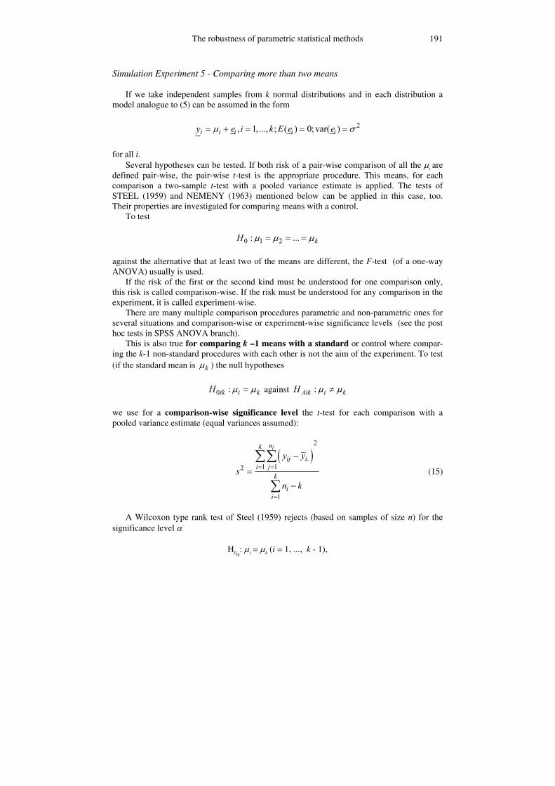
This is also true for comparing k –1 means with a standard or control where compar-ing the k-1 non-standard procedures with each other is not the aim of the experiment. To test (if the standard mean is kµ ) the null hypotheses

0 :ik i kH µ µ= against :Aik i kH µ µ≠

we use for a comparison-wise significance level the t-test for each comparison with a pooled variance estimate (equal variances assumed):

( )2

.1 12

1

ink

ij ii j

k

ii

y y

sn k

= =

=

−

=−

∑∑

∑ (15)

A Wilcoxon type rank test of Steel (1959) rejects (based on samples of size n) for the

significance level α

H0ik: µi = µk (i = 1, ..., k - 1),


if

( ) ( )*max ; 1, ,1 ,S ik ikT W W r k n α= > − − 1,..., 1,i k= − .

For the bounds ( )1, ,1 ,r k n α− − 1,..., 1,i k= − see Steel (1959). The Wik are defined

analogue to (14) and the W*ik are the corresponding values for the inverse rank order. The non-parametric Kruskal-Wallis test in the version of NEMENY (1963) is based on

( )1 1

1 1 , 1,..., 1n n

KW kj ijj j

T R R i kn n= =

= − = −∑ ∑

with the ranks ljR of the j-th element of the l-th sample in the overall ranking of all observa-

tions.

H0ik: µi = µk (i = 1, ..., k - 1) is rejected, if ( ) ( 1) 21; ;1

12KWkn knT d k

nα +

> − ∞ − with

the ( )1; ;1d k α− ∞ − of Dunnett’s test below.

For an experiment-wise significance level we use the Dunnett test (see RASCH et.al., 1999, page 133):

Reject H0ik: µi = µk (i = 1, ..., k - 1) with experiment-wise significance level αe, whenever

2 1 1i. k.

i k > + .y y s

n n

−

d*

holds. The value of d* is for α = 0.05, n1 = n2 = ... = nk-1 = n and nk = n 1k − the value d(k-1;f;0.95) from Table A5 and for nl = n (l = 1,..., k) it is d(k-1;f;0.95) from Table A6 in RASCH et al., 1999.

Again, s2 is a pooled estimator of σ2 with f d.f. RUDOLPH (1985 a,b) compared in a simulation experiment the properties of the Dun-

nett test with those of the test of Steel and Kruskal and Wallis for k = 3, n = 6 and n = 21; α = 0.01 and α = 0.05 and the following variance structures:


Table 5: Variance structures of the simulation experiment

Case 2

1σ 22σ 2

3σ

1 0.5 1 1 2 0.5 0.5 1 3 0.5 2 1 4 2 2 1 5 1 2 1 6 1 1 1

The power was estimated as the relative frequency Pi of rejecting 0 3:ik iH µ µ= (i =1,2)

if

32 2

1 2

ii

nµ µ

σ σ

− ⋅= ∆

+ (16)

Simulation Experiment 6 – Tests for comparing variances

For comparing two variances we assume samples (y 11, ..., y1n1

) and (y21, ..., y2n2) of size n1

and n2 drawn independently from two populations with parameters 21 1 11 12, , ,µ σ γ γ and

22 2 21 22, , ,µ σ γ γ , respectively.

Our purpose is to test the null hypothesis

2 20 1 2:H σ σ=

against

2 21 2:AH σ σ≠

The usual test for comparing two variances is the F-test based on the two sample vari-

ances on the statistic

( )2 21 22 21 2

max( ; )

min ;

s sF

s s=

and to reject H0 if ( )1 21; 1;1F F n n α> − − − , if 2 21 2s s> ; otherwise the d.f. in the F-

quantile have to be interchanged. NÜRNBERG (1982) compared the power of this F-test


with that of 10 further tests (Bartlett, modified Bartlett, modified 2χ , Cochran, Range, Box-

Scheffé, Box-Andersen, Jackknife, Levene-z, Levene-s). We report here only the most im-portant members of this set.

Levene Test: For this test we use the observations y1i and y2i to calculate the quantities

1 1 1 2 2 2;i i i iu y y u y y= − = − for Levene’s z-test

and

( ) ( )2 21 1 1 2 2 2;i i i iv y y v y y= − = − for Levene’s s-test.

Then we carry out an independent samples t-test with the u-values or the v-values for the

z- and s-version of the test, respectively. For the Box-Scheffé-test (also known as Box-test or Box-Kendall-test) (Box, 1953,

Scheffé, 1963) the samples are randomly divided into c groups, c given. These groups con-

tain ijm , 1, 2; 1,...,i j c= = , observations. Let 2ijs denote an estimator of 2

iσ and define

2ln( )ij ijz s= and

2 2

12 2

1 1

2( 1) ( )

( )

iic

ij ii j

c c z zF

z z

⋅ ⋅⋅+ =

⋅= =

− −=

−

∑∑ ∑

The null hypothesis will be rejected if (1,2( 1),1 )F F c α+ > − − . In his simulation

study, Nürnberg (1985) considered the cases 2c = and 3c = .

Simulation Experiment 7 – Tests for the parameters in regression analysis Tests and confidence estimation in linear and quasi-linear (for instance polynomial) re-

gression can be expected to behave like the corresponding inferences for means. Because in psychological research intrinsically non-linear regression – like exponential regression – play no important role, we only summarize the results briefly. The different non-linear re-gression functions investigated in the robustness research are described in Rasch (1995, chapter 16).

In the intrinsically non-linear regression problems arise which are not known in the pro-cedures discussed so far. Parameters can be estimated only iteratively and even for normal distributions the distribution of the estimators (inclusive their expectation and variance) are only known asymptotically (i.e. for a sample size tending to infinity). Therefore we investi-gated together with the robustness also the behaviour of the estimators and the tests for the regression parameters in the normal case for small samples.


Simulation Experiment 8 - Selection procedures As already mentioned in Rasch et al. (1999) and Rasch (2003) selection procedures

should be preferred to multiple comparison because most practical problems are selection problems.

Let us take independent samples from a normal distributions. If the model of the simu-lation experiment 5 is applied, than we are interested to find the greatest value of the expec-tations iµ ( 1,..., )i a= . Without loss of generality, we assume, that

1 2 aµ µ µ≤ ≤ ≤ .

But this order is not known for the user. There are two formulations of this problem:

The Indifference-zone formulation (Bechhofer, 1954) We apply the following selection rule.

Choose that value iµ which belongs to the sample with the greatest mean iy .

In order to describe the error probability we define the event of d-correct selection (dCS):

A dCS occurs, if the selected iµ is greater as a dµ − (Guiard, 1996).

If P(dCS) is the probability of d-correct selection, than 1 ( )P dCSβ = − denotes the

probability of an error. For given values of d and β an appropriate value of n can be calcu-

lated (e.g. Rasch, Herrendörfer, Bock, Victor, Guiard, 1996). We denote a selection rule to be robust if it’s actual error probability Aβ is smaller than

1.2 β⋅ , where β denotes the required error probability. Using other estimations îµ of the

iµ the selection rule can be modified. Following Domröse and Rasch (1987), we get further

selection rules R using the following estimations îµ .

RB: The classical selection rule, RB, proposed by Bechhofer (1954), uses

1

1ˆn

i i ijj

y yn

µ=

= = ∑ .

For normal distributions Rasch (1995) presents tables for planning the sample size n .

RTr0.1 and RTr0.2: The trimmed means (1 )

( )1

1(1 2 )

n

i i jj n

y yn

α

ααα

−

= +=

− ∑ are less sensitive

to outliers. Here ( )i j

y denotes the order statistics (1) (2) ( )i i i n

y y y≤ ≤ ≤ of the variables

ijy , 1,...,j n= . If n α⋅ is not integer, [ ]( 1)i n

yα +

and [ ]( (1 ) 1)i ny

α− + have to be counted by

weights [ ]1 ( )n nα α− − , where [ ]x denotes the integer part of x . We consider the estima-

tors 0,1

î iyµ = for rule RTr0.1, and

0,2î i

yµ = for rule RTr0.2, respectively.


RTi0.1 and RTi0.3: Tiku (1981) proposed the estimators

' ( ) ( 1) ( )1

1ˆ '( )2 2 '

n rT

i ir i j i r i n rj r

y y r y yn r r

µ ββ

−

+ −= +

= = + +

− + ∑ ,

where [ ]0.5 'r r n= + ⋅ and ' ( )( ( ) / ) /= − − ⋅t t t n r n rβ ϕ ϕ (0 ' 1)β< < with t from

1 ( ) /t r n− Φ = . Following Tiku (1981) we use ' 0.1r = , for RTr0.1 and ' 0.3r = for RTr0.3,

respectively. RA: Randlers, Ramberg, and Hogg (1973) described an adaptive selection rule. This rule

works in two steps. In the first step by means of a particular estimator of the kurtosis, the distribution of the data is grouped into one of the three groups „light-tailed“, „medium-tailed“ and „heavy-tailed“. In the second step a selection rule is applied depending on the group, found within the first step.

RRS: The selection rule RRS uses the rank sums 1n

i ijjR r== ∑ instead of îµ , where

ijr denote the rank of ijy among all n a⋅ observations.

For the simulation we apply the so called least favourable configuration:

1 2 1a a dµ µ µ µ−= = = = −

with different values for d . For all other configurations the ( )P dCS would be greater. The

distributions used in the simulation study of Domröse and Rasch (1987) are shown in Table 6.

Table 6:

1 2( , )γ γ -values used in the simulation experiment

type of distribution N U F F F F

1γ = 0 0 0 1 2 - 2

2γ = 0 - 1.2 6 1.5 6 6

N: normal, U: uniform, F: Fleishman Moreover, the following combinations of n and /d σ are used:

n /d σ 11 1; 0.75 21 1; 0.75 47 0.75; 0.5


Subset selection formulation (Gupta, 1956)) The goal of a subset selection procedure consists in selecting a subset, s , of the a distri-

butions such, that the probability ( )P CS , that the „best“ distribution belongs to this subset,

is not smaller than a prespecified value *P . The first of the following selection rules was

developed by Gupta for the case of normal distributions 2( , )iN µ σ :

RG: (Gupta, 1956, 1965) Calculate the sample means iy , 1,...,i a= , and the pooled

variance estimate (15) . Select the distribution i , if

21

1max ( . ., *) 2 /i l a

l ay y t d f P s n−

≤ ≤≥ − .4

Here 1( . .; *)at d f P− denotes the *P -quantile of the ( 1)a − -dimensional t-distribution

with . .d f degrees of freedom and equal correlations 0.5ρ = .

RH: (selection rule of Hsu, 1980): Let 2( ) ( )[1] [n ]

ij ijD D≤ ≤… denote the ordered differences

ig jhy y− ( , 1,..., )g h n= between the samples of the distributions i and j . Then select

distribution i if (ij)[c( *)-n(n+1)/2]min 0Pj i

D≠

> and/or ( )[medium]min 0ij

j iD

≠> , using

( ) 2

( ) [ 1]( ) ( )[medium] 21[ ] [ 1]2

, if 2 1( ) , if =2k

ijij k

ij ijk k

D n kD

D D n+

+

= += +

.

The values ( *)c P are given as ( *)c P rα= (one-tailed, 1 *Pα = − ) in Table VIII of

Miller (1966) RA: The rule RA (Hogg, 1974) is an adaptive selection rule which switches between the

rules GR and HR in dependence of special estimators of skewness and kurtosis and of the

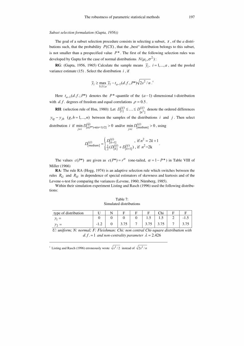
Levene-s-test for comparing the variances (Levene, 1960; Nürnberg, 1985). Within their simulation experiment Listing and Rasch (1996) used the following distribu-

tions:

Table 7: Simulated distributions

type of distribution U N F F F Chi F F

1γ = 0 0 0 0 1.5 1.5 2 -1.5

2γ = -1.2 0 3.75 7 3.75 3.75 7 3.75

U: uniform; N: normal; F: Fleishman: Chi: non central Chi-square distribution with . . 1d f = and non-centrality parameter 2.426λ =

4 Listing and Rasch (1996) erroneously wrote 2 / 2s instead of 22 /s n


In order to estimate ( )P CS , Listing and Rasch (1996) simulated the least favourable

configuration

1 1 aµ µ µ= = = .

For estimating the expected number ( )f d of selected false populations, the configura-

tions

1 2 1a a dµ µ µ µ σ−= = = = − ⋅

with different values of d were simulated.

The number of simulation runs was at least 9000 /sN a= . Listing and Rasch (1996) simulated some further selection rules, but in the present paper only the best ones were de-scribed.

4. Summary of Results and Recommendations We present here the results of the simulation experiments described in paragraph 3. By

Result x we denote the result of simulation experiment x.

Result 1 - One-sample tests and confidence intervals for the mean If we use in definition 1 an ε of 20% of the significance level α = 0.05 , a test is robust

as long as the actual αact lies between 0.04 and 0.06. In Table 8 the minimum sample sizes are given for which a 20% robustness was found.

Table 8:

Sample sizes, which give a 20% robustness

Test No. of distribution in Table 1 and its

1 2, valuesγ γ− − Case a) Case b) Case c)

Test 1 (u) 1 [0; 0],2 [0; 1.5],3[0; 3.75] 5 5 5 Test 1 (u) 4 [0 ; 7],5 [1 ; 1.5],6 [1.5: 3.75] 5 10 10 Test 1 (u) 7 [2; 7] 5 50 50 Test 2 (t) 1 [0; 0],2 [0; 1.5] 5 5 5 Test 2 (t) 3 [0; 3.75] 10 5 5 Test 2 (t) 4 [0 ; 7],6 [1.5: 3.75] 10 50 50 Test 2 (t) 5 [1 ; 1.5] 30 50 50 Test 2 (t) 7 [2; 7] 50 50 50 Test 3 (tJ) 1 [0; 0],2 [0; 1.5] 10 5 5 Test 3 (tJ) 3 [0; 3.75] 50 50 30 Test 3 (tJ) 4 [0 ; 7] 30 50 30 Test 3 (tJ) 5 [1 ; 1.5],6 [1.5: 3.75] 50 30 50 Test 3 (tJ) 7 [2; 7] 50 50 50


It is not surprising that test 3 is quite good if the kurtosis is small. Then it behaves better than the t-test (test 2). But for sample sizes larger or equal to 50 all the tests are 20%-robust.

Result 2 – one-sample sequential tests for the mean The average sample sizes for the 10000 replications did not differ too much for the three

tests if d =1, otherwise they were larger for test 3 than for the other tests. It is known that sequential tests guarantee the risks only approximately even in the normal case. This can be seen from Table 9, but the test is conservative.

Table 9: Percentage of false rejections of H0 for 8 distributions from Table 4 (columns 3 –10) for

α = 0.05, β = 0.2 and d = 0.6

d Test ti 1

[0; 0]

2 [1.006;0.6]

3 [0.35; -0.35]

4 [1.5; 3.75]

5 [0; 3.75]

6 [0; 7]

7 [1; 1.5]

8 [1.5; 3.75]

0.6 1 4.34 7.44 4.93 10.41 3.23 2.95 6.17 7.57 0.6 2 4.64 1.69 3.59 11.11 3.33 2.63 1.78 1.36 0.6 3 4.9 9.18 5.41 12.54 3.33 3.53 7.15 7.02

Table 10: Percentage of false acceptions of H0 for 8 distributions from Table 4 (columns 3 –10 with

[ 21;γγ ]) for α = 0.05, β = 0.2 and d = 0.6

d Test t

i 1 [0; 0]

2 [1.006;0.6]

3 [0.35; -0.35]

4 [1.5; 3.75]

5 [0; 3.75]

6 [0; 7]

7 [1; 1.5]

8 [1.5; 3.75]

0.6 1 15.54 8.95 13.78 5.05 14.64 14.76 10.46 7.24 0.6 2 15.46 27.8 19.45 31.3 13.15 11.53 24.01 27.01 0.6 3 18.9 29.87 21.68 38.84 17.74 16.8 27.21 22.75

The Wald test (test 1) has for the normal distribution (distribution 1) the best approxima-

tion for both risks and is always robust (more than that, conservative) for the risk of the second kind. With exception of the extremely non-normal distribution 2, 4, 7 and 8 it is also robust for the significance level. From the 3 tests examined test 2 must be preferred even if its power is lower than for test 3 (this is a consequence of the higher first kind risk, the power function of test 3 dominates that of test 2 and 1 with exception of distribution 8) in both positions and for all distributions. But for practical distributions in which either the skewness or the kurtosis is low, the test is robust and the average sample size moderate.


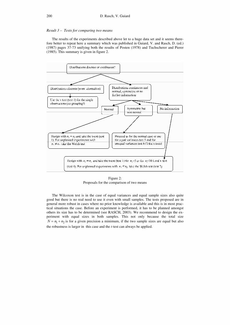
Result 3 – Tests for comparing two means The results of the experiments described above let to a huge data set and it seems there-

fore better to repeat here a summary which was published in Guiard, V. and Rasch, D. (ed.) (1987) pages 37-73 unifying both the results of Posten (1978) and Tuchscherer and Pierer (1985). This summary is given in figure 2.

Figure 2: Proposals for the comparison of two means

The Wilcoxon test is in the case of equal variances and equal sample sizes also quite

good but there is no real need to use it even with small samples. The tests proposed are in general more robust in cases where no prior knowledge is available and this is in most prac-tical situations the case. Before an experiment is performed, it has to be planned amongst others its size has to be determined (see RASCH, 2003). We recommend to design the ex-periment with equal sizes in both samples. This not only because the total size

1 2N n n= + is for a given precision a minimum, if the two sample sizes are equal but also

the robustness is larger in this case and the t-test can always be applied.


Result 4 – Sequential tests for comparing two means For pairwise sampling at each step and if the non-normality of the two populations is of

the same type both tests are conservative for both risks and 20%-robust. The skewness than has nearly no influence on the risks. Pairwise sampling is recommended.

If the non-normality in both populations is different, the skewness influences the risks and the tests are not always robust. Than the kurtosis has no big influence. We think that in practical situations differences in the higher order moments in both populations can not be expected.

For pair-wise sampling in both populations with different probabilities

1 20.75; 0.25π π= = the results are given in Table 11.

Table 11:

Estimated actual risks α̂ and β̂ for Hajnal’s (suffix H) test and the Welch modification

(suffix W) for pairwise sampling and sampling with probabilities 1 20.75; 0.25π π= = ;

d = dW =1.5 are given for α = 0.05 and β = 0.1

Sample 1 Sample 2 pair-wise sampling 1 20.75; 0.25π π= =

1γ 2γ 1γ 2γ ˆHα ˆHβ ˆWα ˆ

Wβ ˆHα ˆHβ ˆWα ˆ

Wβ

0 0 0 0 0.034 0.061 0.031 0.055 0.039 0.067 0.060 0.062 0 1.5 0 1.5 0.036 0.065 0.027 0.064 0.039 0.070 0.061 0.066 0 3.75 0 3.75 0.030 0.067 0.023 0.067 0.037 0.069 0.050 0.065 0 7 0 7 0.022 0.070 0.200 0.068 0.037 0.070 0.044 0.068 0 -1 0 -1 0.038 0.054 0.035 0.055 0.041 0.065 0.091 0.050

0.5 0 0.5 0 0.035 0.058 0.032 0.059 0.041 0.062 0.075 0.043 1 1.5 1 1.5 0.036 0.063 0.026 0.066 0.040 0.058 0.070 0.036

1.5 3.75 1.5 3.75 0.032 0.062 0.024 0.071 0.041 0.059 0.080 0.035 2 7 2 7 0.025 0.070 0.019 0.070 0.039 0.060 0.077 0.034 2 7 0 0 0.046 0.031 0.039 0.093 0.068 0.091 0.071 0.077 0 0 2 7 0.043 0.031 0.038 0.091 0.033 0.025 0.096 0.016 2 7 -2 7 0.095 0.115 0.085 0.119 0.086 0.109 0.122 0.110

Summarizing the results of Table 11 and of further simulation results by Frick (1985) for

unequal variances we propose pair-wise sampling and the Welch modification (test 2) which is also robust in the case of equal non-normality but unequal variances in both populations. Recently it was shown by Häusler (2003) that the triangular sequential test (Schneider, 1992) behaves much better than the tests above. More information will be found in Rasch, Kubin-ger, Schmidtke and Häusler, 2004.


Result 5 – Comparing more than two means For the multiple t-test the robustness is at least as good as for the two-sample t-test, be-

cause robustness increases with the d.f. of the t-test. If the size of each sample is n, the two-sample t-test has 2(n-1) d.f. but in the k-sample case we have k(n - 1) d.f. Therefore no new simulation is needed. This is analogue in the case of comparing with a standard.

That the F-test is very robust against non-normality (but be careful: the F-test for com-paring variances is extremely non-robust, see result 6) was already shown by ITO (1964) and no further simulation was needed. For the many existing multiple comparisons as for in-stance listed under „post hoc tests” in the SPSS ANOVA branch no general recommendation can be given but we think that the Tukey and the Student-Newman Keuls test (based on range) is as robust as the t-test due to the two-sample results for the t- and the Lord (range) test. This will be supported by the poor power results of the rank tests in Rudolph’s experi-ment, where these tests have been compared with the Dunnett-test. The result of Rudolph (1985b) shows that the Dunnett test must be preferred to the rank tests for n< 15, for larger n it is still good but the rank tests behave better than for small samples. For non-normal distri-butions and variance heterogeneity no test is really robust. Here a multiple Welch test may be helpful as in the two-sample problem.

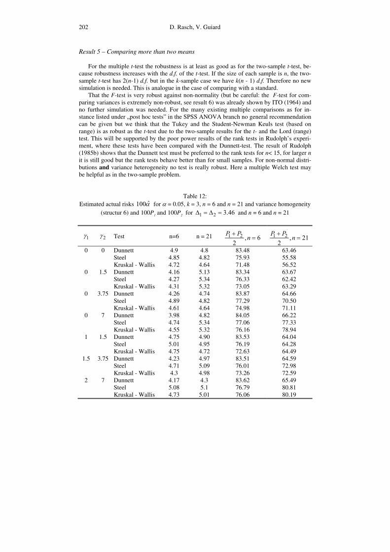
Table 12:

Estimated actual risks ˆ100α for α = 0.05, k = 3, n = 6 and n = 21 and variance homogeneity (structur 6) and 100P1 and 100P2 for 1 2 3.46∆ = ∆ = and n = 6 and n = 21

1γ 2γ Test n=6 n = 21 1 2 , 62

P Pn

+=

1 2 , 212

P Pn

+=

0 0 Dunnett 4.9 4.8 83.48 63.46 Steel 4.85 4.82 75.93 55.58 Kruskal - Wallis 4.72 4.64 71.48 56.52

0 1.5 Dunnett 4.16 5.13 83.34 63.67 Steel 4.27 5.34 76.33 62.42 Kruskal - Wallis 4.31 5.32 73.05 63.29


0 7 Dunnett 3.98 4.82 84.05 66.22 Steel 4.74 5.34 77.06 77.33 Kruskal - Wallis 4.55 5.32 76.16 78.94


1.5 3.75 Dunnett 4.23 4.97 83.51 64.59 Steel 4.71 5.09 76.01 72.98 Kruskal - Wallis 4.3 4.98 73.26 72.59

2 7 Dunnett 4.17 4.3 83.62 65.49 Steel 5.08 5.1 76.79 80.81

Kruskal - Wallis 4.73 5.01 76.06 80.19


We now report some of Rudolph’s results in Table 12. Because P1 and P2 differed only by not more than 0.4 we report the arithmetic mean.

The results can not be interpreted as if the power does not increase with increasing n. From (16) we see that the same ∆ for larger n means a smaller difference in the means. The following conclusion can be drawn. For small samples the Dunnett test is uniformely more powerful than the non-parametric competitors. If the sample size becomes larger, the non-parametric tests are slightly better than the Dunnett test for kurtosis of 3.75 and larger. In Figure 1 those values rather than the rule are the exception and due to the fact that a sample size determination is more easy for the Dunnett test, we see no need to replace this test by a non-parametric one. Furthermore we recommend the selection rules in place of multiple comparisons, not only that they need less number of observations but they are also more robust as shown in Result 7.

Result 6 – Tests for comparing variances Nürnberg (1985) gave the following recommendations: For small sample size n (n=6) only the Box-Scheffé-test (c=2 or 3) is 20%-robust for all

investigated distributions. The F-test for comparing variances should never be used and be deleted from statistical program packages.

For n=18 and 42 the following four tests are 20%-robust: modified Bartlett, Box-Scheffé, Box-Andersen, Levene-s. The other tests are not 20%-robust for some distributions.

SPSS deleted the F-test and replaced it by Leven’s -z-test as part of the procedure in an independent two-samples t-test.

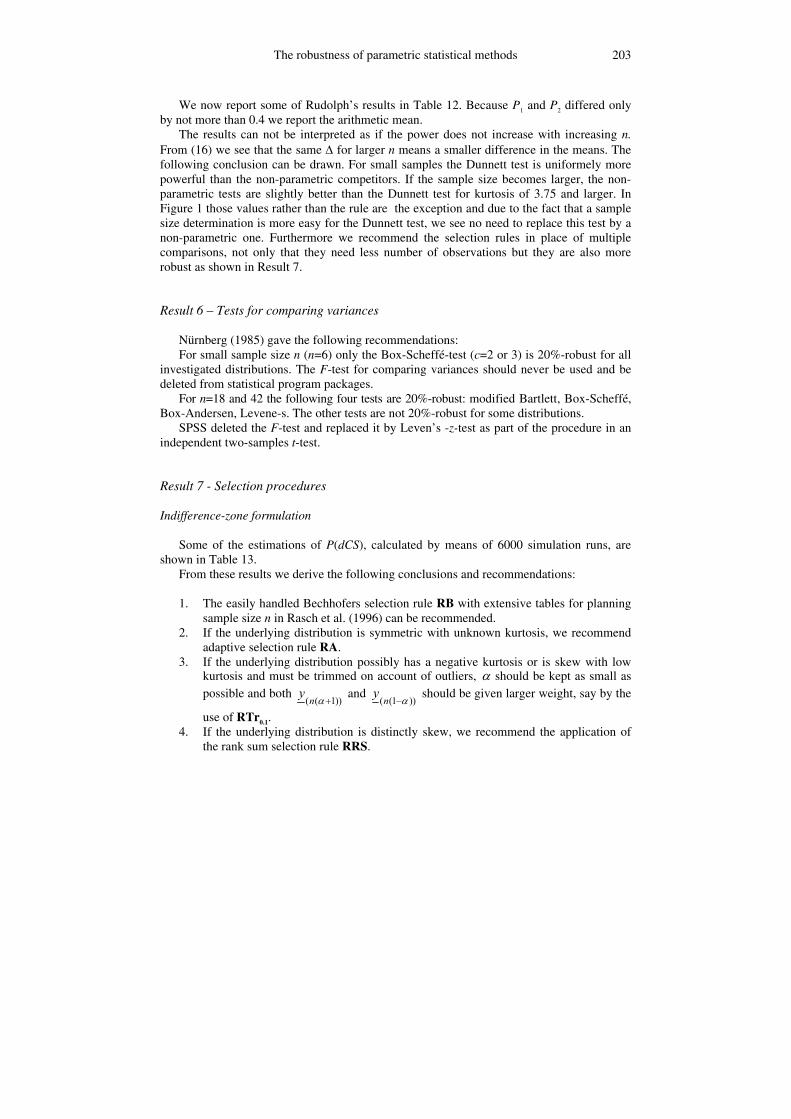
Result 7 - Selection procedures

Indifference-zone formulation Some of the estimations of P(dCS), calculated by means of 6000 simulation runs, are

shown in Table 13. From these results we derive the following conclusions and recommendations: 1. The easily handled Bechhofers selection rule RB with extensive tables for planning

sample size n in Rasch et al. (1996) can be recommended. 2. If the underlying distribution is symmetric with unknown kurtosis, we recommend

adaptive selection rule RA. 3. If the underlying distribution possibly has a negative kurtosis or is skew with low

kurtosis and must be trimmed on account of outliers, α should be kept as small as possible and both

( ( 1))ny

α + and

( (1 ))ny

α− should be given larger weight, say by the

use of RTr0.1. 4. If the underlying distribution is distinctly skew, we recommend the application of

the rank sum selection rule RRS.


Table 13:

Estimates ˆ( )P dCS for different selection rules given 1 0.95β− =

Selection rule

n /d σ 1 0γ = 0 0 1 2 -2

2 1, 2γ = − 0 6 1.5 6 6

RB 21 0.75 0.9553 0.9496 0.9515 0.9454 0.9320 0.9627 47 0.5 0.9533 0.9495 0.9512 0.9392 0.9483 0.9627 RTr0.1 21 0.75 0,8970 0.9425 0.9847 0.9449 0.9605 0.9787 47 0.5 0.8940 0.9405 0.9878 0.9456 0.9635 0.9763 RTr0.2 21 0.75 0.8367 0.9313 0.9903 0.9359 0.9585 0.9810 47 0.5 0.8393 0.9256 0.9907 0.9346 0.9650 0.9790 RTi01 21 0.75 0.9280 0.9423 0.9760 0.9427 0.9485 0.9742 47 0.5 0.9270 0.9442 0.9783 0.9483 0.9557 0.9730 RTi0.2 21 0.75 0.8150 0.9253 0.9893 0.9290 0.9523 47 0.5 0.8168 0.9156 0.9888 0.9244 0.9557 RA 21 0.75 0.9862 0.9483 0.9897 0.9434 0.9335 0.9677 47 0.5 0.9995 0.9495 0.9913 0.9485 0.9412 0.9637 RRS 21 0.75 0.9244 0.9434 0.9867 0.9755 0.9982 0.9844 47 0.5 0.9369 0.9403 0.9884 0.9746 1. 0.9920

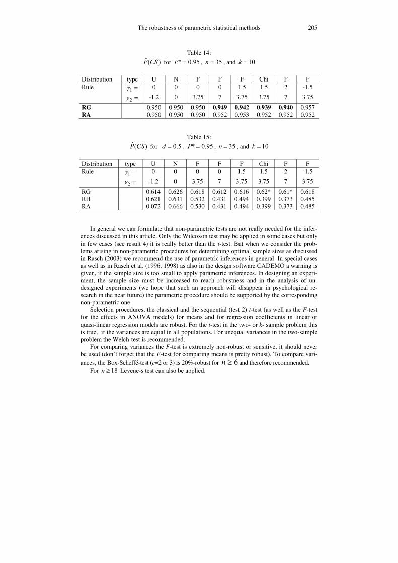
The subset selection formulation: The estimated values of P(CS) for P*=0.95 are shown in Table 14.

In case of ˆ ( ) *P CS P ε< − , this entry was set in boldface. As robustness condition we

use / 5 0.01ε β= = where 1 *Pβ = − denotes the error probability. The estimations of the

expected probabilities, ( )f d , of selecting non-best populations are shown in Table 15. In

the cases where a subset selection procedure fails in robustness we have marked the corre-sponding entry with a „*“ sign.

For the case of equal variances, Listing and Rasch (1996) recommend to use the Gupta rule RG if it is known, that the distributions are approximately normal. If the distributions are completely unknown, the adaptive rule RA should be used.

For the case of unequal variances it was not possible to give a clear recommendation.

5. Final Conclusions We now summarize the recommendations above in some short conclusions. By infer-

ences we mean as well selection procedures, confidence estimations as also hypothesis test-ing. We restrict ourselves on a significance level α = 0.05 or what means the same on a confidence coefficient of 1-α = 0.95 and on a probability of incorrect selection (which plays the role as the α in testing and confidence estimation) of β = 0.05 . Results for α(β ) = 0.01 and α(β ) = 0.1 can be found in the corresponding references.


Table 14: ˆ( )P CS for * 0.95P = , 35n = , and 10k =

Distribution type U N F F F Chi F F Rule 1γ = 0 0 0 0 1.5 1.5 2 -1.5

2γ = -1.2 0 3.75 7 3.75 3.75 7 3.75

RG 0.950 0.950 0.950 0.949 0.942 0.939 0.940 0.957 RA 0.950 0.950 0.950 0.952 0.953 0.952 0.952 0.952

Table 15: ˆ( )P CS for 0.5d = , * 0.95P = , 35n = , and 10k =

Distribution type U N F F F Chi F F Rule 1γ = 0 0 0 0 1.5 1.5 2 -1.5

2γ = -1.2 0 3.75 7 3.75 3.75 7 3.75

RG 0.614 0.626 0.618 0.612 0.616 0.62* 0.61* 0.618 RH 0.621 0.631 0.532 0.431 0.494 0.399 0.373 0.485 RA 0.072 0.666 0.530 0.431 0.494 0.399 0.373 0.485

In general we can formulate that non-parametric tests are not really needed for the infer-

ences discussed in this article. Only the Wilcoxon test may be applied in some cases but only in few cases (see result 4) it is really better than the t-test. But when we consider the prob-lems arising in non-parametric procedures for determining optimal sample sizes as discussed in Rasch (2003) we recommend the use of parametric inferences in general. In special cases as well as in Rasch et al. (1996, 1998) as also in the design software CADEMO a warning is given, if the sample size is too small to apply parametric inferences. In designing an experi-ment, the sample size must be increased to reach robustness and in the analysis of un-designed experiments (we hope that such an approach will disappear in psychological re-search in the near future) the parametric procedure should be supported by the corresponding non-parametric one.

Selection procedures, the classical and the sequential (test 2) t-test (as well as the F-test for the effects in ANOVA models) for means and for regression coefficients in linear or quasi-linear regression models are robust. For the t-test in the two- or k- sample problem this is true, if the variances are equal in all populations. For unequal variances in the two-sample problem the Welch-test is recommended.

For comparing variances the F-test is extremely non-robust or sensitive, it should never be used (don’t forget that the F-test for comparing means is pretty robust). To compare vari-ances, the Box-Scheffé-test (c=2 or 3) is 20%-robust for 6≥n and therefore recommended.

For 18n ≥ Levene-s test can also be applied.


6. References

1. Bechhofer, R.E. (1954): A single-sample multiple decision procedure for ranking means of normal populations with known variances. Am. Math. Statist., 16-39.

2. Bock, J. (1982): Definition der Robustheit. In: Guiard, V. (ed.) 1981, 1-9. 3. Box, G.E.P. & Tiao, G.C. (1964): A note on criterion robustness and inference robustness.

Biometrika 51, 1-34. 4. Domröse, H., Rasch, D. (1987): Robustness of Selection Procedures. Biom. J. 29, 5, 541-553. 5. Feige, K.-D., Guiard, V., Herrendörfer, G., Hoffmann, J., Neumann, P., Peters, H., Rasch, D.

& Vettermann, Th. (1985): Results of Comparisons Between Different Random Number Generators. In: Rasch, D. & Tiku, M.L. (editors): (1985), 30-34.

6. Fleishman, A. J. (1978): A method for simulating non-normal distributions. Psychometrika 43, 521-532.

7. Frick, D. (1985): Robustness of the two-sample sequential t-test. In: Rasch, D. & Tiku, M.L. (editors): (1985), 35-36

8. Guiard, V. (ed.) (1981): Robustheit II – Arbeitsmaterial zum Forschungsthema Robustheit. Probleme der angewandten Statistik, Heft 5, Dummerstorf-Rostock.

9. Guiard, V. & Rasch, D. (ed.) (1987): Robustheit Statistischer Verfahren. Probleme der angewandten Statistik, Heft 20, Dummerstorf-Rostock.

10. Guiard, V. (1996): Different definitions of ∆-correct selection for the indifference zone formulation. J. of Statistical Planing and Inference 54, 175-199.

11. Gupta, S.S. (1956): On a decision rule for a problem in ranking means. Mimeogr. Ser. No. 150, Univ. of North Carolina, Chapel Hill.

12. Gupta, S.S. (1965): On some multiple decision (selection and ranking rules). Technometrics 7, 225-245.

13. Gupta, S.S. & Hsu, J.C. (1980): Subset selection procedures with application to motor-vehicle fatality data in a two-way layout. Technometrics 22, 543-546.

14. Häusler, (2003): Personal communication. 15. Hajnal, J. (1961): A two-sample sequential t-test. Biometrika 48, 65-75. 16. Herrendörfer, G. (ed.) (1980): Robustheit I - Arbeitsmaterial zum Forschungsthema Robustheit.

Probleme der angewandten Statistik, Heft 4, Dummerstorf-Rostock. 17. Herrendörfer, G. & Rasch, D. (1981): Definition of Robustness and First Results of an Exact

Method. Biometrics 37, 605. 18. Herrendörfer, G., Rasch, D. & Feige, K.-D. (1983): Robustness of Statistical Methods. II

Methods for the one-sample problem. Biom. Jour. 25, 327-343. 19. Hogg, R.V. (1974): Adaptive robust procedures: a partial review and some suggestions for

future applications and theory. JASA 69, 909-927. 20. Hsu, J.C. (1980): Robust and nonparametric subset selection procedures. Comm. Statist. Theory

Methods A 9, 1439-1459. 21. Huber, P.J. (1964): Robust estimation of a location parameter. Ann. Math. Statist. 35, 73-101. 22. Huber, P.J. (1972): Robust Statistics: A review. Ann. Math. Statist. 43, 1041-1067. 23. Ito, K. (1969): On the effect of heteroscedasticity and non-normality upon some multivariate test

procedures. Proc. Internat. Symp. Multiv. Analysis vol. 2, New York Academic Press, 87-120. 24. Johnson, N.J. (1978): Modified t-tests and confidence intervals for asymmetric populations.

JASA 73, 536-544. 25. Listing, J., Rasch, D. (1996): Robustnes of subset selection procedures. J. Statist. Planning and

Inference 54, 291-305.


26. Nemeny, P. (1963): Distribution-free multiple comparisons. PhD thesis Princeton Univ., Princeton N.J.

27. Nürnberg, G. (1982): Beiträge zur Versuchsplanung für die Schätzung von Varianzkom- ponenten und Robustheitsuntersuchungen zum Vergleich zweier Varianzen. Probleme der angewandten Statistik, Heft 6, Dummerstorf-Rostock.

28. Nürnberg, G. (1985): Robustness of two-sample tests for variances. In:. Rasch, D. & Tiku, M.L. (editors): (1985), 75-82.

29. Nürnberg, G. & Rasch, D. (1985): The Influence of Different Shapes of Distributions with the same first four Moments on Robustness. In: Rasch, D. & Tiku, M.L. (editors): (1985), 83-84.

30. Mac Laren , M.D. & Marsaglia, G. (1965): Uniform Random Number Generators. J. Assoc. Comput. Mach. 12, 83-89.

31. Mann, H.B. & Whitney, D.R. (1947): On a Test whether One of Two Random Variables is Stochastically Larger than the Other. Ann. Math. Statist. 18, 50-60.

32. Odeh, R.E. & Evans, J.O. (1974): Algorithm AS70: The percentage points of the normal distribution. Appl. Statist. 23, 96-97.

33. Posten, H.O (1985): Robustness of the Two-Sample T-test. In: Rasch, D. & Tiku, M.L. (editors): (1985), 92-99.

34. Posten, H.O (1978): The Robustness of the Two-Sample T-test over the Pearson System. J. of Statist. Comput. and Simulation, 6, 295-311.

35. Posten, H.O. (1982): Two-Sample Wilcoxon Power over the Pearson System. J. of Statist. Comput. and Simulation, 16, 1-18.

36. Randlers, R.H., Ramberg, J.S. & Hogg, R.V. (1973): An adaptive procedure for selecting the population with largest location parameters. Technometrics 15, 769-778.

37. Rasch, D. & Herrendörfer G. (ed.) (1982): Robustheit III - Arbeitsmaterial zum Forschungs- thema Robustheit. Probleme der angewandten Statistik, Heft 7, Dummerstorf-Rostock

38. Rasch, D. (1983): First results on robustness of the one-sample sequential t-test. Transactions of the 9th Prague Conf. Inf. Theory, Statist Dec. Funct., Rand. Processes. Academia Publ. House CAS, 133-140.

39. Rasch, D. (1984): Robust Confidence Estimation and Tests for Parameters of Growth Functions. In: Gyori, I (Ed.): Szamitastechnikai es Kibernetikai Modserek. Alkalmazasa az orvostudomangban es a Biologiaban, Szeged, 306-331.

40. Rasch, D. & Schimke, E. (1985): Die Robustheit von Konfidenzschätzungen und Tests für Parameter der exponentiellen Regression. In: Rasch, D. (ed.) (1985), 40-92

41. Rasch, D. & Tiku, M.L. (editors) (1985): Robustness of Statistical Methods and Nonparametric Statistics. Proceedings of the Conference on Robustness of Statistical Methods and Nonparametric Statistics, held at Schwerin, May 29-June 2, 1983. Reidel Publ. Co. Dortrecht, Boston, Lancaster, Tokyo.

42. Rasch, D. (1985 a): Robustness of Three Sequential One-Sample Tests Against Non- Normality. In: Rasch, D. & Tiku, M.L. (editors): (1985), 100-103.

43. Rasch, D. (1985 b): Robustness of Sequential Tests for Means. Biom. Jour. 27, 139-148. 44. Rasch, D. (ed.) (1985c): Robustheit IV - Arbeitsmaterial zum Forschungsthema Robustheit.

Probleme der angewandten Statistik, Heft 13, Dummerstorf-Rostock. 45. Rasch, D. (1995): Mathematische Statistik. Joh. Ambrosius Barth, Berlin, Heidelberg (851 S.). 46. Rasch, D. (2003): Determining the Optimal Size of Experiments and Surveys in Empirical

Research. Psychology Science, vol. 45 ; suppl. IV ; 3-47. 47. Rasch, D. & Herrendörfer, G. (1981 a): Review of Robustness and Planning of Simulation

Experiments for its Investigation. Biometrics 37, 607.


48. Rasch, D. & Herrendörfer, G. (1981 b): Robustheit statistischer Methoden. Rostocker Math. Kolloq. 17, 87-104.

49. Rasch, D., Herrendörfer, G., Bock, J., Victor, N. & Guiard, V. (1998): Verfahrensbibliothek Versuchsplanung und -auswertung. R. Oldenboug Verlag München Wien, Band I 1996; Band II 1998.

50. Rasch, D., Kubinger, K., Schmidtke, J. & Häusler (2004): Use and misuse of Hypothesis Testing. In preparation.

51. Rasch, D., Verdooren, L.R., Gowers, J.I. (1999): Fundamentals in the Design and Analysis of Experiments and Surveys – Grundlagen der Planung und Auswertung von Versuchen und Erhebungen. R. Oldenburg Verlag München Wien.

52. Reed A.H. & Frantz, M.E. (1979): A Sequential Two-Sample t-Test using Welch Type Modification for unequal variances. Comm. Statist. A –Theory and Methods, 14, 1459-1471.

53. Rudolph, P.E. (ed.) (1985 a): Robustheit V - Arbeitsmaterial zum Forschungsthema Robustheit. Probleme der angewandten Statistik, Heft 15, Dummerstorf-Rostock.

54. Rudolph, P.E. (1985 b): Robustness of many-one statistics. Rasch, D. & Tiku, M.L. (editors): (1985), 128-133.

55. Schneider, B. (1992): An Interactive Computer Program for Design and Monitoring of Sequential Clinical Trials. International Biometric Conference 1992, Hamilton, New Zealand, Invited Paper Volume.

56. Steel, R.G.D. (1959): A multiple comparison rank sum test. Biometrics, 15, 560-572. 57. Teuscher, F. (1979): Ein hierarchischer Pseudo-Zufallszahlengenerator. Unpublished paper at

the research centre Dummerstorf-Rostock. 58. Teuscher, F. (1985): Simulation Studies on Robustness of the t- and u- Test against Truncation

of the Normal distribution. In: Rasch, D. & Tiku, M.L. (editors): (1985), 145-151. 59. Tiku, M.L. (1980): Robustness of MML estimators based on censored samples and robust test

statistics. J. Statist. Planning and Inference, 4, 123-143. 60. Tiku, M.L. (1981): Testing linear contrasts of means in experimental design without assuming

normality and homogeneity of variances. Invited paper presented at the March 22 to 26, 1981 Biometric Colloquium of the GDR-Region of the Biometric Society.

61. Tiku, M.L. (1982): Robust statistics for testing equality of means or variances. Comm. Statist Theory Methods A 11, 2543-2558.

62. Tuchscherer, A. (1985): The robustness of some procedures for the two-sample location problem – a simulation study (concept). In: Rasch, D. & Tiku, M.L. (editors): (1985), 159-164.

63. Tuchscherer, A. & Pierer, H. (1985): Simulationsuntersuchungen zur Robustheit verschiedener Verfahren zum Mittelwertvergleich im Zweistichprobenproblem (Simulationsergebnisse). In: Rudolph, P.E. (ed.) (1985 a), 1-42.

64. Verdooren, L.R. (1963): Extended tables of critical values for Wilcoxons test. Biometrika, 50, 177-185.

65. Wald, A. (1947): Sequential Analysis. John Wiley, New York. 66. Welch, B.L. (1947): The Generalization of Student’s Problem when Several Different

Population Variances are Involved. Biometrika, 34, 28-35. 67. Wilcoxon, F. (1945): Individual Comparisons by Ranking Methods. Biometrics, 1, 80-82. 68. Zielinsky, R. (1977): Robustness: a quantitative approach. Bull. Laced. Polonaise de Science,

Ser. Math., Astr. et Phys., Vol. XXV, 12, 1281-1286.

Documents

The robustness of parametric statistical methods - Pabst · The robustness of parametric statistical methods 177 Experimenters know that they nearly never really meet observations