The Risk-Return Characteristics and Diversification

Claremont CollegesScholarship @ Claremont

CMC Senior Theses CMC Student Scholarship

2017

The Risk-Return Characteristics andDiversification Benefits of Fine Wine InvestmentTania SalomonClaremont McKenna College

This Open Access Senior Thesis is brought to you by Scholarship@Claremont. It has been accepted for inclusion in this collection by an authorizedadministrator. For more information, please contact [email protected].

Recommended CitationSalomon, Tania, "The Risk-Return Characteristics and Diversification Benefits of Fine Wine Investment" (2017). CMC Senior Theses.1668.http://scholarship.claremont.edu/cmc_theses/1668

http://scholarship.claremont.edu

http://scholarship.claremont.edu/cmc_theses

http://scholarship.claremont.edu/cmc_student

mailto:[email protected]

Claremont McKenna College

The Risk-Return Characteristics and Diversification Benefits of Fine Wine Investment

submitted to Dean Janet Kiholm Smith

and Professor Manfred Keil

by Tania Salomon

for

Senior Thesis Spring 2017

April 24, 2017

ABSTRACT

This thesis evaluates the risk-return characteristics and diversification benefits of fine wine

investment. It compares the historical performance of wine to that of equity, fixed income, real

estate, and commodities. I calculate the correlation, volatility, and expected returns of these

assets to examine whether adding wine to a portfolio increases its risk-adjusted return. I do this

through the Markowitz portfolio optimization technique. The findings suggest that wine has a

low correlation with traditional assets, providing diversification benefits. My results also show

that adding wine to a portfolio increases its risk-adjusted return only when there is an allocation

constraint of 0 to 25% per asset. This does not hold, however, when there are no asset allocation

constraints.

ACKNOWLEDGEMENTS

This thesis would not have been possible without the guidance of Professor Janet K. Smith. Professor, you showed interest in my project from the very beginning and gave me the motivation and advice I needed to write this thesis. I appreciate your support from the bottom of my heart. Also, many thanks to Professor Yu who gave me the tools and technical knowledge necessary to write this thesis. There are not enough words to thank my writing advisor, Mellissa Martinez. She not only helped me edit the 15,000 ‘financy’ words of this thesis but also every single one of my papers throughout my undergraduate education. Mellissa, I would have not survived these past four years without your support. I am grateful to you for teaching me the true power of writing. I would also like to thank Professor William Ascher. Bill, thank you for showing me that there is much more than Finance out there. You taught me to think in a philosophical manner, while always keeping the practical solution in mind. I will always value the analytical curiosity that you sparked in me. Another person that played a huge role in my college education was Professor Marc Massoud. Dad, you motivated me to explore, discover, and pursue my professional passions. You showed me what a person who loves his job looks like. Your dedication to students is truly incredible and I hope that one day I can inspire someone to learn as much as you motivated me to learn. Thanks to all my professors, in general. I would not be the person I am today without having been exposed to your classes, and having absorbed as much knowledge as I did throughout my years at CMC. I cannot thank enough to Annushka Shivnani. Girlie, few words can describe how much I enjoyed those late-night conversations and the many times we could not stop laughing. Thanks for making me listen to the other side of the story. The combination of your intellectual curiosity and sense of humor shaped my college experience. I could not have asked for a better best friend. I would also like to thank David Magun. Thanks for pushing me to be the best version of myself; for challenging me intellectually; questioning my arguments; and for continuously motivating me every time I complained about my workload. Thank you for literally standing by my side every weekend I had to work for the last three semesters. Last but not least, thanks to my family. Pao, thanks for being my role model. Your common sense, social skills, and positive vibes have enabled me to look at life through a different lens. There are no words to describe how much you inspire me to excel personally and professionally. Jonathan and Alan, thanks for always believing that I can accomplish whatever goals I set for myself. Mom, thanks for your warmth and for instilling in me the value of learning. Dad, thanks for teaching me to never give up and to analyze things in a way that would help me better understand the bigger picture.

Two years ago, I interned at a wealth management firm in San Diego, CA as an Equity

Research Analyst. It was then that I realized how difficult it is for people to diversify their

lifelong savings. Equity and fixed income markets are known to be sound investments in the

context of a diversified portfolio. However, customers are constantly looking for more ways to

diversify. What investment alternatives are available? This was a question I asked myself

continuously and it remained unanswered even after my internship had ended. As I was listening

to a world-class sommelier teaching at a Restaurant Management program in Switzerland, one

potential solution came to me: wine.

“If you buy a Chateau de XYZ today, it can be worth 20 times more in 10 years,” the

sommelier said. Since my sister was about to graduate from High School, I thought it would be a

good idea to buy a bottle of wine as a present, and tell her that she could either drink it or sell it

in 10 years. However, I also wondered, what if she does not know how to keep a wine bottle?

What if she does not manage to maintain the right temperature and humidity? After that, I came

to the conclusion that instead of buying one bottle, I could buy a collection of 100 bottles. And

instead of doing this only for my sister, I could offer the service to several customers and make a

business out of it. Could it be possible that wine is not only the best thing to complement a meal,

but also a viable way to increase a portfolio’s risk-adjusted return and diversify one’s

investments?

Table of Contents I. Introduction............................................................................................................................. 1 II. The Market for Wine Investment........................................................................................... 2 III. Literature Review................................................................................................................. 6 IV. Data Description................................................................................................................. 11 V. Analysis............................................................................................................................... 15 VI. Results................................................................................................................................ 17 VII. Conclusion........................................................................................................................ 29 VIII. Discussion........................................................................................................................ 30 IX. Tables................................................................................................................................. 34 X. Appendix............................................................................................................................. 56

1

I. Introduction

Given that the current markets face uncertainty caused by global political polarization, all-time

low interest rates, and an all-time high value of the U.S. Dollar, investors are hungry for

innovative investments that will provide diversification benefits and high returns. Although some

authors believe that these two parameters are mutually exclusive, I hypothesize that, in the case

of fine wine investment, they go hand-in-hand. More specifically, this thesis evaluates whether

fine wine offers higher risk-adjusted return than equity, fixed income, commodities, and real

estate, and if it provides diversification benefits when added to a portfolio. My research attempts

to answer three questions regarding the characteristics of fine wine as an investment:

1. Does fine wine offer higher risk-adjusted returns than equity, fixed income, commodities,

and real estate?

2. Does fine wine provide a diversification benefit? If so, for what type of wine investment

is this benefit more pronounced: highly demanded wines or frequently invested wines?

3. What is the optimal portfolio allocation between equity, fixed income, commodities, real

estate, and fine wine?

The answers to these questions provide information for investors to make financial

decisions. This study analyzes the performance of the mentioned asset classes over the period of

2006 to 2016. The data comes from well-recognized indices with high trading volumes. The

structure of this thesis is as follows: First, I provide a background for the market of wine

investment and a literature review. These two sections are followed by a data description, an

explanation of the financial analyses performed, and an interpretation of the results. The research

concludes with a discussion of the results and final remarks. I apply methodology similar to that

of McGah’s (2009) work on art investment. My analysis begins with an evaluation of the risk-

2

and-return1 trade-offs of different asset classes (equity, fixed income, commodities, real estate,

and wine). Each asset is then priced with the single-index model to calculate its alpha

(idiosyncratic risk factors) and beta (asset's market risk). These betas are then plugged into the

capital asset pricing model (CAPM) to get the expected returns of each asset. Furthermore, I

perform a correlation analysis to analyze the diversification benefits of wine. The final section of

the project determines optimal portfolios based on the expected returns, correlation, and

volatility of each of the assets. To do this, I use the Markowitz (1952) portfolio optimization

technique, which produces various minimum-variance portfolios.

II. The Market for Wine Investment

A. Ways to Invest in Wine

There are a variety of ways that one can invest in wine. Options include the following:

buying highly-rated bottles on Amazon and storing them in one's own cellar; purchasing high-

end bottles on a wine-exchange;2 hiring a broker to trade and properly store them;3 arbitraging4

bottles of a specific vintage between auction houses in different parts of the world; investing in

equity of a mutual fund that offers wine investment services to its clients (such as WAM

Capital);5 crowdfunding on a wine project;6 en premier buying (wine futures) which involves

securing a price before the wine is bottled; and even trading weather derivatives to hedge for

1 This is measured by the Sharpe ratio, or the average return earned in excess of the risk-free rate per unit of volatility or total risk. The higher the ratio, the more attractive the investment. 2 Such as the global leading wine exchange: London International Vitners Exchange or “Liv-ex.” 3 An example of a storage service is the one provided by Vinfolio. They inspect and store the bottles in a professional temperature and humidity controlled environment (Vinfolio Website). 4 Arbitrage refers to the simultaneous purchase and sale of an asset to profit from a difference in the price. 5 Australian Securities Exchange: WAM. http://www.wamllp.com/. 6 The American Association of Wine Economics reported that, based on a survey, crowdfunding wine projects is appealing to the younger generations (Bargain et. al, 2016). Kickstarter-like sites for wine are: Naked Wines, Fundovine, and Cruzu.

3

fluctuations in wine prices (Yandel, 2012). There are currently no existing wine indices to invest

in. During my interview with Greg Smart, a Research Analyst at Liv-ex in London, I learned that

one cannot directly invest in the Liv-ex indices at present and there are no derivatives directly

linked to the indices.

B. Wine Investment

On a general level, research shows that individual wines and direct investments have a

higher risk than common indices with differing return levels (Devine & Lucey, 2015). While

scholars do not address transaction and storage costs in detail, these parameters do have a

substantial impact on wine investment. For example, while the Liv-ex charges 2-3% per trade,

Vinfolio Storage Services charge approximately 1.5% of the wine portfolio size. Buying from

primary markets, or directly from the vineyard, removes the trading fees. At a more specific

level, Dimson (2014) says that high-quality wines that are still maturing provide the highest

financial return, while widely-recognized wines offer a quantifiable non-financial benefit to

owners.

C. Background of Wine Trading

The wine market consists of two main branches: early consumption (those consumed

within three years of release), which accounts for 90% of the market, and investment-grade

wine,7 which has a highly liquid secondary market (Kumar, 2005). Before the existence of the

Internet, but more specifically, before Liv-ex, wine pricing was subjective, depending on

differing commissions and fees of auction houses. Not everyone had full access to historical and

current prices. However, the emergence of electronic trading, combined with the laws of supply

7 Investment-grade wines are also known as the blue-chips. These are those from: Bordeaux, Burgundy, Rhone Valley, Tuscany, Piedmont and Champagne.

4

and demand, have fueled the standardization of pricing, and hence wine trading. Most wine

investors monitor price changes on the Liv-ex to execute trades, as this platform offers a

transparent and reliable valuation system that captures the trading conditions prevalent in the

market.

D. Industry Today

In recent years, the wine investment industry has grown consistently, perhaps, due to

positive global economic conditions in the post-financial crisis years. Before the 90s, demand

mainly came from Europe and the U.S. (Beck, 2008). Today, however, demand from Asian

investors (mainly from Singapore and Hong Kong) is at an all-time high. In 2008, Hong Kong

abolished the tax on wine and now holds the second largest wine auction center in the world.

This has fueled the industry to reach high growth levels. Emerging markets like China, India and

Russia have shown increased interest in wine as well. Wine has existed for millennia, and based

on history, I suspect demand will continue to increase at even higher growth rates.

The supply side of the equation is far more interesting. Not only is there a fixed supply of

every investment grade vintage, which decreases once it matures and becomes consumed, but

crop yields also reduce as vineyards choose quality over quantity (Beck, 2008). I contend that

since the wine market is not priced with total efficiency, investors can benefit from scarcity as

demand will continue to increase.8 A fixed supply and an increasing demand means higher

prices, and hence, higher returns for investors. Lastly, profit from wine is exempt from capital

gains tax in the majority of countries, which makes it attractive for investors. The fine wine

8 Fine wine is not a perfect capital market, as it entails transaction costs price uncertainty due to subjective ratings and changes in consumer preferences.

5

investment industry will continue to grow in the long-term as price discovery becomes more

transparent and returns remain attractive.9

E. Who Should Invest in Wine?

This project suggests that wine investment should be considered by those who are

looking for an alternative investment.10 This type of investment can sometimes entail high

volatility, but there is debate in the field regarding wine’s level of risk. Once on the market, wine

prices are strongly influenced by reviews from prominent sommeliers or wine critics, like Robert

Parker.11 Some argue that wine investment might be too risky for those who are looking for an

ultra-safe portfolio. In fact, five years ago, the U.K.’s Financial Services Authority suggested

that financial advisers should only advise customers with income and capital above specific

levels to consider taking the risk in “Unregulated Collective Investment Schemes,” which are

usually a component of wine funds (Northrop, 2012). However, some research states that wine

can significantly lower volatility in a portfolio (Mahesh, 2007). This paper seeks to further

investigate these claims. Whether wine investment is for wine lovers, high-risk investors, well-

diversified investors, or those who are looking for diversification is yet to be determined.

9 Email interview with Greg Smart, Research Analyst at Liv-Ex, London, February 6th, 2017. 10 An alternative investment refers to one that is not conventional such as stocks, bonds, or cash. 11 Robert Parker is a leading American wine critic with strong international influence.

6

III. Literature Review

There has been much debate regarding whether or not wine is a sound alternative

investment, and if it offers diversification benefits. Almost 40 years ago, Labys and Cohen

(1978) examined data on wine yield and risk analysis using Christie’s auction data. In their

research, they compare the return on wine investment to a variety of debt instruments and

medium-term financial assets and conclude that “one should buy wine for the purpose of

consumption rather than for investment.”

Dimson et al. (2014) analyze the impact of aging on Premiers Crus Bordeaux wine prices

and the long-term investment performance of fine wine. They find that young high-quality wines

that are still maturing, provide the highest financial return, while widely-recognized wines offer

a quantifiable non-financial benefit to owners. They use an arithmetic repeat-sales regression

over 1900 to 2012. This method calculates changes in the sales price of the same asset over time.

The researchers estimate a real financial return to wine investment of 4.1%, which according to

them, exceeds government bonds, art, and investment-quality stamps. They find that wine

appreciation is positively correlated with stock market returns.

There has also been research regarding the diversification effects of wine investment.

Unlike Dimson et al., Kun Chu (2014) finds that wine has a low correlation with stock

investments, and infers that it may provide a diversification benefit. He uses well-known fine

wine indices (Liv-ex Fine Wine Bordeaux 500 and 100) to test diversification benefits within a

portfolio. The results show that while Liv-ex100 may provide a diversification benefit in an

investment portfolio, Liv-ex500 does not, as it has a causal relationship with most of the stock

market indexes. Additionally, their results imply that fine wine investors may anticipate the stock

market movements and change their investment amounts in fine wine accordingly.

7

Burton and Jacobsen (2001) calculate the rate of return from holding red Bordeaux wine

from 1986 to 1996 using repeat-sale regression. They further contrast wine performance on an

aggregate basis and for several portfolios to that of other asset classes. Their results support the

idea that wine does not yield greater returns than financial assets, especially when the volatility

of returns and transaction costs are taken into account.

Years later, Devine and Lucey (2015) find different results. They analyze the returns of

Bordeaux and Rhone wines through a repeat-sales regression method. Their findings suggest that

these wine regions can provide average returns in excess of risk-free investments with lower risk

at the index level. They do not mention whether their analysis controls for transaction costs.

Individual wines, sub regions, and direct investments involve a higher risk than the general

indices with varying return levels. Furthermore, inexperienced, low volume or individual

investors carry a high level of risk when investing in wine. Returns on indirect investment via

wine funds vary. However, all average returns of funds exceed the general Rhone and Bordeaux

Index in this research. They conclude that volatility for some wine funds is high and might not

suit risk-averse investors.

Fogarty (2005) develops a guide for wine pricing with the hope that there is an

opportunity for wine investment in Australia. He uses different approaches for the indices

including: a multiplicative chain price, a geometric mean price, a repeat-sales approach

regression, a hedonic price equation approach, and an auction house (Langton’s) fine wine index.

He suggests that hedonic pricing is the best possible way to value wine. Hedonic pricing assumes

that it is possible to completely describe the underlying attributes of the product in question. He

claims that in the context of wine, it is therefore assumed that the price of a bottle sold at an

auction reflects its value of time, vintage, rating, grape variety, and region. Six years later, he

8

proposes the “hybrid model,” an improved approach to estimate the returns from wine. He claims

that the hybrid model is better as it uses all available data, unlike the repeat sales model;

moreover, this model identifies repeat sales where they exist, unlike the hedonic model (Fogarty

& Jones, 2011).

Fogarty (2007) focuses on both investment feasibility and portfolio risk reduction of

wines from the perspective of an investor in the UK and Australia. He analyzes his data through

a repeat-sales approach, and concludes the following: “vintage wine indexes understate the

return a typical investor receives; comparisons using pre-tax returns overstate the value of

standard financial assets relative to wine; and wine investment provides value by reducing the

risk of a given portfolio.” In 2010, he confirms that although Australian wine shows a lower

return than standard financial assets, it provides a modest diversification benefit.

Masset and Weisskopf (2010) take a more specific approach than hedonics to value wine.

They use hammer auction prices (1996 to 2009) from The Chicago Wine Company to examine

wine’s risk, return, and diversification benefits. However, they give special focus to periods of

economic downturn. They build their own wine indices for different regions and prices using

repeat-sales approach regressions. Their results suggest that fine wine yields a higher return and

has a lower volatility compared to stocks, especially in times of economic crises, as wine returns

are primarily related to economic conditions and not to the market risk. Not only are returns

favorably impacted and risk minimized but skewness and kurtosis are also positively affected.

Masset and Henderson (2012) evaluate auction data reported at the Chicago Wine

Company from 1996 to 2007. They find that the best wines according to characteristics like

vintage, rating and ranking earn higher returns and tend to have a lower variance than poorer

wines. Their results indicate interesting individual performance of wine in terms of risk-return

9

trade-off and low correlation with equities. This suggests that wine has attractive diversification

benefits. They also conclude that investors should diversify across different wine categories as

wine short-run movements are partially independent of each other. Finally, first growths (top

Bordeaux wines) and wines rated as extraordinary by Robert Parker deliver the best tradeoff in

terms of portfolio expected returns, variance, skewness and kurtosis for most investor preference

settings under consideration.

A few years later, Masset and Weisskopf (2014) looked into the performance of wine

funds, specifically the ability of managers to display selectivity and market timing. They find

that for a U.S. investor, wine funds offer rather poor returns but may be interesting from a

diversification perspective. Out of nine funds they analyze, only one fund manager shows

positive risk-adjusted returns, while another manager appears to time the wine market

successfully. They conclude that, considering non-quantifiable risks, wine funds do not appear to

be worthwhile investments.

The most recent studies on wine investment were performed by Bouri (2015). He uses a

multivariate model to examine the return relations between equity indices from several

developed countries (U.S., UK, Germany, France, Japan) and fine wine prices. He finds that

wine has a hedging ability against most equity indices. As opposed to Masset and Weisskopf

(2010), Bouri does not find evidence supporting wine’s safe haven role in economic downturns.

A year after, Bouri and Roubaud (2016) focus on co-movements between fine wine and stock

prices in the UK. Using data from 2001 to 2014, they conclude that fine wine is a hedge asset12

against movements in UK stocks, but not a safe heaven13 for market turmoil.

12 A hedge asset refers to an asset that does not co-move—negatively correlated or uncorrelated—with a portfolio in times of stress. 13 A safe heaven refers to a loss reducer in extreme adverse market conditions.

10

All in all, several studies over the last three decades have analyzed the added value of

wine in a given portfolio. Some results have supported the idea of wine investment (Dimson et

al., 2015; Lucey & Devine, 2015; Masset & Hendersen, 2010; Masset & Weisskopf, 2010),

while others have found evidence questioning its merits (Burton & Jacobsen, 2001; Labys &

Cohen, 1978). Furthermore, some researchers have found results that support the idea of the

diversification benefits of wine (Bouri, 2015; Bouri & Roubaud, 2016; Fogarty, 2007; Fogarty,

2010; Kun Chu, 2014; Masset & Hendersen, 2010; Masset & Weisskopf, 2010; Masset &

Weisskopf, 2014), while others have found the opposite (Dimson et al. 2015).

The purpose of my study is to analyze the 10-year historical performance of fine wine

and evaluate whether it is an attractive alternative investment that provides diversification

benefits. The previous literature has analyzed data through 2014. This work differs from

previous studies in that it analyzes data through late 2016, it incorporates historical prices from

secondary market indices, and it offers optimal portfolio allocations between equity, fixed

income, commodities, real estate, and fine wine.

11

IV. Data Description

I use monthly data from March 2006 to August 2016 from Wharton Research Data

Services (WRDS), Federal Reserve Economic Data (FRED), and Bloomberg. I convert each

asset class data into percentage changes, using STATA for my regressions. Table 3 shows the

summary statistics.

A. Fine Wine Prices

Based on “Sources of Wine Economic Data,” from the Journal of Wine Economics, I

concluded that the most useful sources for the purpose of my analysis were Liv-ex100 and Liv-

exFWI (Fine Wine Investables). I was not able to add fine wine auction prices for my analysis.

While Sotheby’s informed me that they could not share data, Christie’s ran me through the

process of data acquisition. However, it was extremely difficult to aggregate their data as very

few wines with the same label, and from the same vintage, sold consistently every month. I also

tried to include the Wine Spectator Auction Index, a composite of average prices for 32 of the

most sought-after wines in today's auction market. However, even though Wine Spectator

mentions (on their web page) that the prices are updated on a “regular basis,” the index only

provides data through the third quarter of 2014. After reaching out to them, I learned that they

would not update their data before I completed this project. Lastly, Vivino, Wine-searcher, and

Vinfolio did not respond to my requests. After much time and effort spent gathering data, I

determined that data for fine wine prices should come from the most well-known indices (Kun

Chu, 2014): the Liv-ex100 Fine Wine Index (Liv-ex100) and the Liv-ex Fine Wine Investables

Index (Liv-exFWI). The London International Vintners Exchange (Liv-ex), a global wine trading

platform, tracks both indices.

12

A.1. Highly Demanded Wine

I measure highly demanded wine using the Liv-ex100 index, which is the industry's

leading benchmark. This represents the price movement of 100 of the most desirable fine wines

for which there is a strong secondary market. Wines in this index must have attracted high

approval ratings from a leading critic (a 95-point score or above) and should be available in the

UK market. The majority of the index consists of Bordeaux wines, but it also includes wines

from Burgundy, the Rhone, Champagne and Italy. Liv-ex calculates the index using mid prices

(the highest bid price and lowest offer price on the trading platform) from live transactions in

their global trading platform for fine wine. The index weighs a combination of price, production

and scarcity. Although the company reviews the component wines quarterly, when a wine

reaches 25-years from vintage, they remove it from the index as volumes are too low for a strong

secondary market.14 See Appendix A for a detailed list of wines that comprise this index.

A.2. Commonly Invested Wine

The other measure of wine is the Liv-exFWI (Fine Wine Investable) index, which tracks

wines frequently found in wine investment portfolios. The index contains Bordeaux reds from 24

leading chateaux.15 Some bottles date back to the 1988 vintage and are chosen depending on

their score from Robert Parker. The wines must have also scored 95-points or above. However,

the big eight of Bordeaux—the five First Growths,16 Ausone, Cheval Blanc and Petrus—are

included on the basis of a score of 93 or above. Liv-ex prices the wines by also using mid prices.

It also calculates the index monthly. Scarcity weightings are applied to the older vintages and to

14 Liv-ex Web page 15 Château comes from the French word, “castle.” In the European Union, a bottle labeled as a chateau wine means that the grapes are solely from the vineyard of the property. Most wineries buy grapes outside their property, so this is a way to emphasize the opposite. In the U.S., this term is mostly used as marketing strategy. 16 Château Lafite Rothschild, Chateau Latour, Chateau Margaux, Chateau Haut-Brion, and Chateau Mouton Rothschild

13

those produced in smaller quantities. The component wines are reviewed twice a year.17 See

Appendix B for a list of wines that comprise this index.

B. Equity

B.1. U.S. Equity

U.S. equity data comes from the Standard and Poor's 500 Index (SPX). The SPX is an

index that tracks large-cap American equities. It is a market capitalization-weighted index, which

monitors the return on 500 stocks representing all major industries in the United States. The

sector weightings as of March 2017 are as follows: Technology 20%, Financials 16%, Health

Care 15%, Consumer Discretionary 13%, Industrials 10%, Consumer Staples 10%, Energy 8%,

Materials 3.25%, Utilities 3%, and Telecom 2%. I use U.S. equity to evaluate the optimal

allocation between all asset when I create the portfolios. I later perform a robustness check

running the same analysis, but also with international and emerging markets equity.

B.2. International Equity

International equity data comes from Morgan Stanley Capital International (MSCI)

EAFE Index. This is a float-adjusted market capitalization index that tracks the performance of

large and mid-cap securities in 21 developed economies, excluding the U.S. and Canada. The

countries included are: Austria, Belgium, Denmark, Finland, France, Germany, Ireland, Israel,

Italy, Netherlands, Norway, Portugal, Spain, Sweden, Switzerland, U.K., Australia, Hong Kong,

Japan, New Zealand, and Singapore.

B.3. Emerging Markets Equity

Emerging Markets (EM) equity data comes from the MSCI EM Index. This is a float-

adjusted market capitalization index that measures the market performance of equity in 23

17 Liv-ex Web page

14

emerging economies, including: Brazil, Chile, China, Colombia, Czech Republic, Egypt, Greece,

Hungary, India, Indonesia, Korea, Malaysia, Mexico, Peru, Philippines, Poland, Qatar, Russia,

South Africa, Taiwan, Thailand, Turkey, and the UAE.

C. Fixed Income

Fixed income data comes from indices tracking the performance of U.S. Generic

Government 10 year yields, which refer to yield-to-maturity and are pre-tax. They are based on

the ask side of the market and are updated daily. The rates are comprised of Generic United

States on-the-run government bill/note/bond indices.

D. Commodities

Commodities data originates from The Deutsche Bank Liquid Commodity Index

(DBLCI), which monitors the performance of six commodities in the energy, precious metals,

industrial metals and grain sectors. The commodities that comprise this index are: WTI crude oil,

heating oil, aluminum, gold, corn and wheat. The DBLCI weighs each of these depending on the

price movement of the underlying commodity futures.

E. Real Estate

Real estate data comes from an equal-weighted index using residential and commercial

real estate data.18 Residential real estate data comes from the Case-Shiller Housing Price Index.

This monitors U.S. residential prices with a repeat-sales approach, following changes in the

value of residential real estate nationally, as well as, within 20 metropolitan regions. Commercial

real estate data comes from Green Street’s Commercial Property Price Index, which is formed by

a time series of current and historical unlevereged commercial property values in the U.S.

18 Similar approach to that of McGah (2009).

15

V. Analysis

My numerical analysis consists of two main processes: assessing and comparing the

historical risk-adjusted return each asset; and using the Markowitz portfolio optimization

technique to build minimum-variance portfolios, while maximizing risk-adjusted returns. The

Sharpe ratio measures the excess return (or risk premium) per unit of risk (or a deviation risk

measure). For the first section of the paper, this is calculated as follows:

𝑆ℎ𝑎𝑟𝑝𝑒𝑅𝑎𝑡𝑖𝑜 = - . /012

(1)

where the E(R) is equivalent to the arithmetic mean of the past 126 monthly returns for each

asset (to reflect its historical returns), 𝑟3 is the risk-free rate that applies to the period, and σ is the

standard deviation of the asset throughout the period. For the second segment of the paper, E(R)

is calculated using the expected returns from the single-index model and capital asset pricing

model (CAPM). I describe this process below.

The Markowitz portfolio optimization technique requires the input of expected returns for

each asset class. In order to calculate these, I use the single-index model, which estimates the

sensitivity (or beta) coefficient of a security to systematic risk using a single-variable linear

expression. I use a common proxy for systematic risk, the S&P 500 (Bodie, Kane, & Marcus,

2008), to denote the market. Regressing the excess return of a security 𝑅419 on the excess return

of the market index 𝑅520 generates the following equation:

𝑅4 = 𝛼 + 𝛽𝑅5 + 𝜀 (2)

Here, α is the excess return of security ‘i’ when the market excess is zero, β is the slope

coefficient or the security beta, and ε is the residual. Because the expected return of ε is zero, one

19 𝑅4 = 𝑟4 − 𝑟3, where 𝑟4 is the return of the security and 𝑟3 is the risk-free rate. 20 𝑅5 = 𝑟;&=>?? − 𝑟3.

16

can assume that:

𝐸(𝑅4) = 𝛼𝑖 + 𝛽𝑖𝐸(𝑅5) (3)

Similar to the previous equation, alpha reflects the non-market premium. A large alpha

might suggest that the security is underpriced. The second term of Equation 3 indicates the

degree to which the security returns covary with the market. After performing this analysis for

each asset class (equity, fixed income, commodities, real estate, and wine), I calculate the

Markowitz expected returns by plugging each beta into the CAPM equation:

𝐸 𝑅4 = 𝑟3 + 𝛽𝑖[𝑀𝑅𝑃] (4)

Historically, long-term market risk premium (MRP) has been 7.5% per year (Officer and

Bishop, 2008). I therefore use 0.63%21 as a constant for my assumptions. Regarding the risk-free

rate, I use the 2007 to 2016 average 3-month T-bill, and convert it to monthly.22 After calculating

the expected return for each asset, I plug the input into the Markowitz portfolio optimization

model. This model looks for the optimal asset allocation to maximize the portfolio’s Sharpe

ratio, considering each asset’s expected return (E(𝑅4)), variability (standard deviation), and the

correlations between each other.

In order to see the effect of wine on an investment portfolio, I use four types of portfolios

with different asset classes included. The asset classes in each portfolio are summarized in Table

1. Furthermore, I create different scenarios by placing constraints on the asset allocation weights,

as few investors are willing to heavily invest in only one asset class. Hence, I create three

scenarios with different weight ranges (0% - 100%, 0%-35%, and 0% - 25%) between the asset

classes for each of the portfolios. It was imperative that the sum of the weights add up to one and

21 7.5% ÷ 12𝑚𝑜𝑛𝑡ℎ𝑠 = 0.63% 22 0.73% ÷ 12𝑚𝑜𝑛𝑡ℎ𝑠 = 0.06%

17

were not negative (no short-selling). In sum, I create a total of twelve different portfolios, which

are summarized in Table 1.

After the main analysis, I further perform a robustness check. Since I use U.S. equity (ie.

S&P500) as the sole equity asset class in the previous calculations, I decide to run the Markowitz

optimizer for the twelve portfolios again, while including emerging markets and international

equity as potential asset classes. Table 1b summarizes the assets included in each of the twelve

portfolios from the robustness check.

VI. Results

A. Main Analysis

A. 1. Returns Analysis

My results show that wine has had higher monthly returns than equity, fixed income, real

estate, and commodities over the last decade (see Table 3). The arithmetic and geometric average

returns are as follows: wine (Liv-ex100) 0.68% and 0.63%, wine (Liv-exFWI) 0.84% and 0.80%,

U.S equity 0.50% and 0.41%, EM equity -0.22 and -0.82%, international equity 0.02% and -0.13,

fixed income -0.43% and -0.88%, commodities -0.18% and -0.35%, and real estate 0.14% and

0.13%. Compared to the other assets, wine has the second to lowest standard deviation (Liv-

ex100 0.031 and Liv-exFWI 0.027) after real estate (0.013). This suggests that wine exhibited

lower volatility than equity, fixed income, and commodities throughout this period. Lastly,

historically, wine has higher Sharpe ratios (Liv-ex100 0.185 and Liv-exFWI 0.292) than the

other assets (U.S. equity 0.095, emerging markets equity -0.024, international equity 0.004, fixed

income -0.093, commodities -0.060, real estate 0.098). As previously mentioned, a higher Sharpe

ratio reflects a greater return per unit of risk.

18

A.2. Single-Index Model

Regarding the single-index model, the beta of EM equity was significant at the 5% level

and that of international equity was not significant. Besides these, all of the other betas (U.S.

equity, fixed income, real estate, and commodities) were significant at the 1% level except for

that of Liv-exFWI. This indicates that wine, measured by the Liv-exFWI, is not correlated with

the market. Similarly, wine measured by the Liv-ex100 has a really low beta (0.061). This idea

suggests that although the asset moves in the same direction as the S&P 500 (has a positive

beta), it also has a low systematic risk, meaning that wine has a low correlation with the market.

These results suggest that wine is a good alternative asset for diversification purposes. The rest

of the assets also exhibit positive betas. All traditional assets (equity, fixed income, real estate,

and commodities) have statistically insignificant alphas. Interestingly, however, both measures

of wine have significant alphas. The Liv-ex100 alpha was significant at the 10% level and the

Liv-exFWI alpha was significant at the 1% level. These high alphas suggest that wine has beaten

the benchmark (SPX), having higher returns than U.S. equity. Refer to Table 4 for a summary of

the single-index model alphas and betas.

The last step in the computation of the expected returns of each asset uses the betas

calculated above and plugs them into Equation 4. From this, I calculate the following monthly

expected returns: wine (Liv-ex100) 1.4%, wine (Liv-exFWI) 0.5%, U.S equity 7.6%, EM equity

4.5%, international equity 1.3%, fixed income 4.9%, real estate 0.8%, and commodities 5.3%.23 I

then input them into the Markowitz optimizer. Table 5 shows the calculations and assumptions

for these computations.

23 Wine’s (10-year) arithmetic returns are higher than those of traditional assets. Wine’s expected returns (calculated with CAPM) are much lower than those of traditional assets. See the Discussion section for a potential explanation of why this is true.

19

A.3. Correlations24

Next, I develop an asset correlation matrix, which is also needed for the Markowitz

optimizer. A correlation between two assets reflects the degree of relationship of their

movements; a correlation of 1 suggests that the returns of the assets fluctuate in tandem; a

correlation of -1 implies that prices move in opposite directions; a correlation of 0 means that the

price movements of assets are uncorrelated, or that the movements of one asset have no effect on

those of the other asset. Either a negative correlation or a zero correlation (or not statistically

significant) is regarded as positive for diversification purposes. The asset correlations can be

seen in Table 6. The following correlations regarding wine exist at the 1% level: the two

measures of wine are significantly correlated (0.27) for obvious reasons. Wine (Liv-ex100) and

equity are barely correlated (0.23), suggesting that wine goes in the same direction as the S&P

500. This correlation is lower than the correlation between fixed income and equity (0.29). Given

that investors usually use fixed income as a hedge for movements in equity, the correlation

between Liv-ex100 and equity suggests that wine can be also used to hedge for changes in the

equity market. The same reasoning can be used for commodities. Furthermore, wine neither

significantly correlates with international equity, nor with emerging markets equity. Lastly, there

is no significant correlation between the Liv-ex100 and fixed income. These results suggest that

wine, measured by the Liv-ex100, may provide diversification benefits as it shows to be a hedge

asset. Similarly, the other measure of wine (Liv-exFWI) is negatively correlated with fixed

income at the 10% level, meaning that they move in opposite directions. Apart from this, no

other correlations regarding this wine index are significant.

24 This is a detailed description of the correlation results. Skip to Implications for investment on page 26 for a summary.

20

The correlations suggest that both measures of wine provide diversification benefits.

However, the Liv-exFWI is even more beneficial, as it is uncorrelated with all traditional assets,

and negatively correlated with fixed income. In sum, wine investment serves as a hedge against

movements in traditional assets. Since one can look at the asset correlation to see whether or not

wine is good for diversification (Fogarty, 2010 & Kun Chu, 2014), my results suggest that wine

does provide diversification benefits from an asset correlation perspective.

A.4. Asset Allocation 25

Finally, I employ the Markowitz (1952) technique to build minimum variance optimal

portfolios. I use the previously calculated expected returns, standard deviations, and asset

correlations to create several portfolios. This process helps assess whether adding wine to a

portfolio increases returns, while also minimizing risk. As mentioned in the Analysis section,

there are four portfolios with different asset classes: portfolio 1 includes all assets (equity, fixed

income, real estate, and commodities) but wine; portfolio 2 contains all assets plus the Liv-

ex100; portfolio 3 incorporates all assets plus the Liv-exFWI; and portfolio 4 includes all assets

plus the Liv-ex100 and the Liv-exFWI. Table 1 shows the assets included in each of the four

portfolios. Furthermore, there are three scenarios (portfolio types) for each of the portfolios with

varying constraints on allocation weights (type-X: 100% ≥ w ≥ 0%, type-Y: 35% ≥ w ≥ 0%, and

type-X: 25% ≥ w ≥ 0%). Table 2 shows the weight constraints applied to each portfolio.

Results from the main analysis support my hypothesis to a large extent. Introducing fine

wine into a portfolio that already contains equity, fixed income, real estate, and commodities

increases its risk-adjusted return. This is only true, however, when there are restrictions placed

on the maximum allocation of each asset. In other words, the Sharpe ratio increases as I add wine

25 This is a detailed description of the optimal asset allocation results. Skip to Implications for investment on page 26 for a summary.

21

to a portfolio, only under the scenarios with allocation constraints of 0-35% and 0-25% per asset.

This can be, perhaps, explained by the fact that the benefit of wine’s low volatility outweighs its

relatively low expected returns. Under the scenarios with no restrictions on allocation (0 to

100%), the expected returns of the portfolios increase as I add wine, while the Sharpe ratio

declines. A higher Sharpe ratio represents a greater return per unit of risk, and vice-versa. Tables

7 through 10 summarize the optimizer’s output regarding each portfolio’s asset allocation,

expected return, standard deviation, and Sharpe ratio. As shown in Table 7, the expected returns

and Sharpe ratios of the portfolios without wine (portfolios X1, Y1, and Z1) are 0.51% and

0.157, 0.43% and 0.133, and 0.44% and 0.106, respectively.

In the next three portfolios, I add highly demanded wine (Liv-ex100) as an asset class.

Table 8 summarizes the optimal asset allocation, expected returns, and Sharpe ratios for

portfolios X2, Y2, and Z2. Although the optimizer does not include wine in portfolio X2, which

shows expected return of 0.51% and a Sharpe ratio of 0.157, portfolios Y2 and Z2 do

recommend adding the Liv-ex100 into the portfolio. 26 Y2 and Z2 show expected returns of

0.37%, and Sharpe ratios of 0.143 and 0.123, respectively. Even though the expected returns for

the type-Y27 and type- Z28 portfolios decrease as I add wine, their Sharpe ratios are higher than

those without wine. These results suggest that under a 0-100% allocation constraint, adding fine

wine in the form of the Liv-ex100 to a portfolio does not increase its risk-adjusted return.

However, adding wine to a portfolio under a 0-35% allocation constraint increases its risk-

adjusted return by 7.5%. Moreover, a portfolio with a 0-25% allocation constraint highly benefits

from including this asset, as its risk-adjusted return increases by 16%.

26 Portfolio Y2 recommends a 20% wine allocation; portfolio Z2 suggests a 25% wine allocation. 27 Type-Y portfolios are those with a 0 to 35% asset allocation constraint. 28 Type-Z portfolios are those with a 0 to 25% asset allocation constraint.

22

In the next three portfolios, I remove the Liv-ex100, and include commonly invested wine

(Liv-exFWI). Table 9 summarizes the optimal asset allocation, expected returns, and Sharpe

ratios for portfolios X3, Y3, and Z3. Portfolio X3 includes only a 1% wine allocation, showing a

higher expected return than X1 (no wine portfolio), but a lower Sharpe ratio of 0.145. Most

importantly, Y3 and Z3 show slightly lower expected returns, but much higher Sharpe ratios than

the portfolios without wine, with 0.135 and 0.121, respectively. These results suggest that

following a 0-100% allocation constraint, including the Liv-exFWI to a portfolio increases its

expected return by 23%, but does not increase its risk-adjusted return. Conforming to a 0-35%

allocation constraint, adding fine wine in the form of the Liv-exFWI to a portfolio increases its

risk-adjusted return by only 1.5%. A portfolio with a 0-25% allocation constraint, on the other

hand, highly benefits from including wine, as its risk-adjusted return increases by 14%.

Lastly, I create three more portfolios including all traditional assets and both the Liv-

ex100 and the Liv-exFWI. Table 10 summarizes the optimal asset allocation, expected returns,

and Sharpe ratios for portfolios X4, Y4, and Z4. The returns and Sharpe ratios for these

portfolios are as follows: 0.63% and 0.145, 0.36% and 0.136, and 0.33% and 0.123, respectively.

Here, the results from adding wine mirror those of the previous six portfolios in that the expected

return of the portfolio with no asset allocation constraint (0-100%) increases, while its Sharpe

ratio declines. On that basis, the portfolios with asset allocation constraints of 0-25% and 0-35%

show a higher Sharpe ratio as I add both measures of wine. Some might argue that the portfolios

with asset allocation constraints better represent the effect of wine on an investor’s portfolio, as

only very few investors are willing to allocate most of their capital to a single asset. However, I

am unsure about this, as most investors do not place asset allocation constraints below 25% per

23

asset. Table 11 summarizes the expected returns, standard deviations, and Sharpe ratios of the

twelve portfolios.

In sum, as I add wine to an X-type portfolio the expected returns increase, while the

Sharpe ratio does not. This suggests that adding wine to a portfolio restricted to a 0 to 100%

allocation is not necessarily beneficial when the main goal is to maximize risk-adjusted return.

From the four Z-type portfolios, those with the highest return per unit of risk are Z2 and Z4 with

expected returns and Sharpe ratios of 0.37% and 0.123, and 0.33% and 0.123, respectively. The

portfolio with the lowest return per unit of risk is the portfolio without any wine included, or Z1,

with a Sharpe ratio of 0.106. Regarding the Y-type portfolios, those with the highest Sharpe

ratios are Y2 and Y4, with Sharpe ratios of 0.143 and 0.136, respectively. Table 12a through 12c

reflect the asset allocations of the portfolios with the highest and lowest Sharpe ratios under each

asset allocation constraint. Table 12a shows that expected returns increase as I add wine to the

portfolios, while the Sharpe ratios decline. Table 12b and 12c reflect that the portfolios with the

highest Sharpe ratios are those that include all of the assets plus the Liv-ex100, and those that

include both wine measures. Furthermore, only including the Liv-exFWI is not as optimal as the

previous combinations, but is still better than having no wine at all.

B. Robustness Check

As previously mentioned, I perform a robustness check to corroborate the effects of

adding wine to a portfolio. Although the results of the main analysis support my hypothesis to a

large extent, those of the robustness check only partially confirm my findings. Since I use

S&P500 as the sole equity asset class in the main analysis, I re-run the Markowitz optimizer for

the twelve portfolios, including emerging markets and international equity as potential asset

classes. Similar to the main analysis, the robustness check consists of four portfolios with

24

different asset classes: portfolio I includes all assets (U.S. equity, emerging markets equity,

international equity, fixed income, real estate, and commodities) but wine; portfolio II contains

all assets plus the Liv-ex100; portfolio III incorporates all assets plus the Liv-exFWI; and

portfolio IV includes all assets plus the Liv-ex100 and the Liv-exFWI. Here, there are also three

scenarios for each of the portfolios with varying constraints on allocation weights (type-X: 100%

≥ w ≥ 0%, type-Y: 35% ≥ w ≥ 0%, and type-Z: 25% ≥ w ≥ 0%). The summary of the assets and

allocation constraints of the twelve new portfolios can be seen in Tables 1b and 2.

The results from the robustness check are similar to those of the main analysis in that

introducing wine to a portfolio that has 0 to 25% asset allocation constraint increases its risk-

adjusted return. The results are not as conclusive when it comes to an allocation constraint of 0 to

35%. They support my findings that adding wine to a portfolio restricted to a 0 to 100%

allocation is not necessarily beneficial when one tries to maximize a portfolio’s risk-adjusted

return. Tables 13 through 16 summarize the optimizer’s output regarding each portfolio’s asset

allocation, expected return, standard deviation, and Sharpe ratio. As shown in Table 13, the

expected returns and Sharpe ratios of the portfolios without wine (portfolios X-I, Y-I, and Z-1)

are 0.63% and 0.146, 0.41%, and 0.133, and 0.43% and 0.115, respectively.

Following the main analysis methodology, in the next three portfolios, I add highly

demanded wine (Liv-ex100) as an asset class. Table 14 summarizes the optimal asset allocation,

expected returns, and Sharpe ratios for portfolios X-II, Y-II, and Z-1I. Portfolio X-II only gives a

1% allocation to wine, showing an expected return of 0.64% and a Sharpe ratio of 0.146.

Portfolios Y-II and Z-1I include larger portions of wine (14% and 16% wine allocations,

respectively) and show expected returns and Sharpe ratios of 0.43% and 0.131, and 0.39% and

0.126, respectively. This proposes that adding Liv-ex100 to a portfolio with a 0 to 25% asset

25

allocation constraint increases its risk adjusted return by 9.6%. Interestingly, the opposite effect

happens in portfolio Y-II with a 0 to 35% asset allocation constraint. As I add wine to Y-I, its

expected return increases by 5%, while its Sharpe ratio slightly declines by 1.5%.

In the next three portfolios, I remove the Liv-ex100, and include commonly invested wine

(Liv-exFWI). The results are consistent with the previous ones. Table 15 summarizes the optimal

asset allocation, expected returns, and Sharpe ratios for portfolios X-III, Y-III, and Z-1II.

Portfolio X-III shows nearly the same results as X-I (no wine portfolio). Although portfolios Y-

III and Z-1II show slightly lower expected returns (0.39%, and 0.36%, respectively) than the

portfolios with no wine, their risk-adjusted returns are higher (0.135 and 0.128, respectively).

Again, this suggests that adding the Liv-exFWI to a Z-type portfolio increases the risk-adjusted

return by 11%, as the Sharpe ratio grows from 0.115 to 0.128. Similarly, adding the Liv-exFWI

to a Y-type portfolio increases the risk-adjusted return by 1.5%.

Lastly, I create three more scenarios including all the assets and both the Liv-ex100 and

the Liv-exFWI. Table 16 summarizes the optimal asset allocation, expected returns, and Sharpe

ratios for portfolios X-IV, Y-IV, and Z-1V. The returns and Sharpe ratios for these are as

follows: 0.50% and 0.145, and 0.39% and 0.133, and 0.35% and 0.129, respectively. Results

under these scenarios are somewhat different from those of the main analysis. X-IV shows both a

lower expected return and a slightly lower Sharpe ratio after adding wine. Z-1V shows a lower

expected return, but a higher risk-adjusted return. Y-IV shows a lower expected return, and an

unchanged Sharpe ratio as both wines are included. Table 17 shows a summary of the expected

returns and Sharpe ratios of the portfolios created in the robustness check.

In the robustness check, type-X and type-Y portfolios do not conclusively benefit from

adding wine. Table 18a through Table 18c show the asset allocations, Sharpe ratios, and

26

expected returns for each of the portfolio types. The results manifest in three different ways.

While portfolio X-II follows a similar movement to that of the main analysis (higher expected

return, and unchanged Sharpe ratio as wine is added),29 X-III and X-IV do not. As wine is added,

the expected return of X-III slightly decreases, while its risk-adjusted return remains unchanged.

For portfolio X-IV, both the expected return and the Sharpe ratio decline. All the X-type

portfolios in the main analysis supported the fact that adding wine to a portfolio with a 0 to 100%

asset allocation constraint increases its expected return, while decreasing its Sharpe ratio. The

results from the robustness check do not uphold my findings. From this, I decide that the overall

results of my study only partially support my hypothesis. Regarding the Z-type portfolios, these

follow the same trend as those in the main analysis in that adding wine increases the portfolio

risk-adjusted return, while also bearing a lower expected return. The Y-type portfolios show

conflicting results to those of the main analysis. Adding the Liv-ex100 to a portfolio with a 0 to

35% asset allocation constraint increases the expected return, while slightly decreasing the

Sharpe ratio. Adding the Liv-exFWI instead, increases the portfolio’s risk-adjusted return while

bearing a decline in the expected return. Adding both measures of wine decreases the expected

return, while the Sharpe ratio remains the same. These last results suggest that following a 0 to

35% allocation constraint, a combination of both wines is not recommended.

C. Implications for investment

First, this thesis addresses the question of whether wine is correlated with other assets.

Either a negative correlation or a zero correlation (or not statistically significant) are regarded as

positive for diversification purposes. The correlations suggest that both measures of wine

29 As I add wine, the main analysis shows a lower Sharpe ratio when expected returns are higher.

27

provide diversification benefits. However, the Liv-exFWI serves more as a hedge asset, as it is

uncorrelated with all traditional assets, and negatively correlated with fixed income.

This thesis also tackles the question of whether adding wine to a portfolio increases its

risk-adjusted return. The results from the main analysis show a trend of an increasing risk-

adjusted return and a decreasing expected return as I add wine to portfolios with 0-25% and 0-

35% asset allocation constraints. Additionally, as I add wine to a portfolio conforming to a 0 to

100% asset allocation constraint, the expected returns of the portfolios increase, while the Sharpe

ratios either remain the same or decrease. The results from the robustness check partially mirror

those of the main analysis. These also show that as I add wine to portfolios with a 0 to 25% asset

allocation constraint, their risk-adjusted return increases. This is also the case for portfolios with

an asset constraint of 0 to 35%, but only when the Liv-ex100 is added. When the Liv-exFWI or

both wines are added to these portfolios, their risk-adjusted returns decline. Additionally,

portfolios with asset allocation constraints of 0 to 100% do not show an increase in risk-adjusted

returns as I add wine. These calculations support the fact that adding wine to a portfolio

restricted to a 0 to 100% allocation is not beneficial when one tries to maximize a portfolio’s

risk-adjusted return. In sum, the answer to the prevalent question (could it be possible that wine

is not only the best thing to complement a meal, but also a viable way to increase a portfolio’s

risk-adjusted return and diversify one’s investments?) is: it depends. Even though wine has had

much higher historical returns than any other traditional asset (see Table 5) throughout the last

decade, adding wine might or might not be beneficial when seeking a risk-adjusted return

maximization. Whether adding wine to a portfolio has a positive or negative impact on its risk-

adjusted return depends on the circumstances of the portfolio to which the wine is added, in

addition to investor preferences.

28

Table 19 shows the asset allocations of the portfolios with the highest Sharpe ratio for

each type of investor. Assuming that investors are looking for a portfolio with the maximum

risk-adjusted return, from the 24 portfolios created throughout this project, we can conclude the

following: If investors are willing to allocate up to 100% of their capital into one asset, they

should choose the allocation suggested in either portfolio X1 or X2. If investors desire to allocate

up to 35% of their capital into one asset, they should choose the allocation suggested in portfolio

Y2. If investors want to allocate up to 25% of their capital into one asset, they should choose the

allocation suggested in portfolio Z-1V. In fact, the results from this study suggest that adding

wine to a portfolio of an investor with these preferences increases its risk-adjusted returns.

29

VII. Conclusion

The results from the arithmetic and geometric returns (Table 3) are consistent with the

literature that supports wine as an investment (Dimson et al., 2015; Lucey & Devine, 2015;

Masset & Hendersen, 2010; and Masset & Weisskopf, 2010). Over the last ten years, wine has

had higher returns than equity, fixed income, real estate and commodities. Throughout this time

period, wine has also shown lower volatility than all of these assets, except for that of real estate.

Perhaps, because of this, wine shows higher risk-adjusted returns than all of the traditional assets

included in the analysis.

Furthermore, assuming that a zero correlation between wine and a traditional asset

implies that wine provides diversification benefits (as it serves as a hedge asset) my results

comport with the conclusions of the literature supporting the diversification benefits of wine

(Bouri, 2015; Bouri & Roubaud, 2016; Fogarty, 2007; Fogarty, 2010; Kun Chu, 2014; Masset &

Hendersen, 2010; Masset & Weisskopf, 2010; Masset & Weisskopf, 2014). I find that wine only

slightly correlates with U.S. equity and does not correlate with all the other assets, including

international and emerging markets equity, fixed income, commodities, and real estate. Lastly,

based on the findings from the Markowitz portfolio optimizer, I conclude that adding wine30 to a

portfolio that already contains equity, fixed income, real estate, and commodities, and with a 0 to

25% asset allocation constraint, increases its risk-adjusted return. This is also true as I add the

Liv-ex100 to portfolios under a 0-35% asset allocation constraint. However, my results suggest

that a portfolio’s risk-adjusted return does not increase in portfolios conforming to a 0 to 100%

asset allocation as I add wine. One may argue that a 0 to 25% asset allocation constraint is more

realistic than 0 to 100%, as few investors are willing to place most their capital into only one

30 Either in the form of Liv-exFWI, Liv-ex100, or both

30

asset. However, even if most investors do not want to allocate most of their capital into one asset,

in reality, only few investors place restrictions below 25% per asset. This argument also holds

true for the 0 to 35% asset allocation constraint. From this, I conclude that wine investment is for

wine lovers rather than risk-adjusted return maximizers.

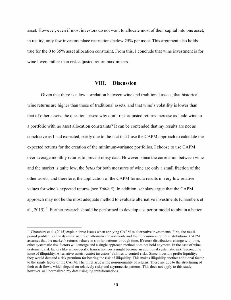
VIII. Discussion

Given that there is a low correlation between wine and traditional assets, that historical

wine returns are higher than those of traditional assets, and that wine’s volatility is lower than

that of other assets, the question arises: why don’t risk-adjusted returns increase as I add wine to

a portfolio with no asset allocation constraints? It can be contended that my results are not as

conclusive as I had expected, partly due to the fact that I use the CAPM approach to calculate the

expected returns for the creation of the minimum-variance portfolios. I choose to use CAPM

over average monthly returns to prevent noisy data. However, since the correlation between wine

and the market is quite low, the betas for both measures of wine are only a small fraction of the

other assets, and therefore, the application of the CAPM formula results in very low relative

values for wine’s expected returns (see Table 5). In addition, scholars argue that the CAPM

approach may not be the most adequate method to evaluate alternative investments (Chambers et

al., 2015).31 Further research should be performed to develop a superior model to obtain a better

31 Chambers et al. (2015) explain three issues when applying CAPM to alternative investments. First, the multi-period problem, or the dynamic nature of alternative investments and their uncommon return distributions. CAPM assumes that the market’s returns behave in similar patterns through time. If return distributions change with time, other systematic risk factors will emerge and a single approach method does not hold anymore. In the case of wine, systematic risk factors like wine-specific transaction costs might become an additional systematic risk. Second, the issue of illiquidity. Alternative assets restrict investors’ abilities to control risks. Since investors prefer liquidity, they would demand a risk premium for bearing the risk of illiquidity. This makes illiquidity another additional factor to the single factor of the CAPM. The third issue is the non-normality of returns. These are due to the structuring of their cash flows, which depend on relatively risky and asymmetric patterns. This does not apply to this study, however, as I normalized my data using log transformations.

31

estimate of wine’s expected return relative to other assets. I speculate that in such a case, the

conclusions could have confirmed my hypothesis.

There are some limitations to my findings. In the first part of my numerical analysis, the

Sharpe ratio utilizes historical returns. Given that my results are time-sensitive, one cannot be

completely certain that the sound performance and volatility of wine as an investment will

continue to be as profitable and stable as in the past decade. Perhaps fluctuations in wine’s

supply and demand will take place in the years to come. For example, we may see changes in

consumer preferences or wine production. Also, academics might dispute that illiquid

investments lower a portfolio's standard deviation, as those investments prove to be less volatile.

However, I argue that fine wine is not as illiquid as one might assume. The fact that the wine

trading industry is much smaller than that of equity32 or fixed income does not mean that the

asset cannot quickly turn into cash. There are online platforms (consider E-trade but for fine

wine) where investors can easily trade wine on a daily basis.33 Liv-ex expanded from handling

1% of the global wine trades in 2000 to 2.5% in 2009.34 Furthermore, in 2009, the global wine

industry sales totaled 3 billion dollars. Based on the assumption that this amount grew by the

same rate of inflation, which is a fairly conservative assumption, 2016 fine wine sales were 3.8

billion dollars.35 Lastly, skeptics can challenge my findings in that the 𝑅X of wine from the

single-index model are low. Some think that the alpha and beta of assets with 𝑅X figures below

0.50 are unreliable because the assets are not sufficiently correlated to make a worthwhile

comparison. However, I argue that a low 𝑅X or beta does not necessarily make an investment a

32 Global volume of equity in 2015 totaled 99.7 trillion dollars (World Bank). 33 Liv-ex is the most well-known wine trading platform 34 Ram, Vidyia, Forbes, July 2009. 35 If the market share of Liv-ex increased at the same rate it did from 2000 to 2009, Liv-ex yearly trading would account for 190 million dollars.

32

poor choice. The betas calculated from the single-index model are low, which are interrelated

with 𝑅X and the correlation between the asset and its benchmark.36 Simply put, a low 𝑅X means

that its performance is statistically unrelated to its benchmark. In fact, this supports the claim of

wine offering diversification benefits.

It is important to emphasize that this work does not factor in asset transaction costs

(trading fees and storage costs in the case of wine) into the numerical analysis. Although the

historical returns of wine were high in this research, investors should analyze whether these costs

outweigh the returns. On average, private wealth managers charge 1.0% to 2.0% of the account

value per year. Wine, however, has a broader range. Trading platforms charge approximately 2%

to 3% per trade, and storage services cost approximately 1.5% of the wine portfolio size per year.

I suspect that such high transaction costs might explain the large discrepancy between CAPM

expected returns and average returns. Investors demand a premium from bearing high transaction

costs, which might be embedded in wine’s high returns. This claim is consistent with that of

Chambers et al. (2015).

Furthermore, there are non-quantifiable factors that play into one’s decisions to invest in

wine. Fine wine investment might seem like an esoteric endeavor. If a client feels that she knows

nothing about wine, she might be reluctant to invest in it. On the other hand, there is a potential

convenience yield that arises from owning wine. I argue that there is an “elite” aspect of wine

ownership that may enhance the personal satisfaction of owning a bottle collection.

Lastly, one of the main reasons that I wanted to investigate the potential of wine as an

investment was because I thought it might be a business opportunity. As mentioned in the

Market for Wine Investment section, there are multiple ways in which one can invest in wine.

36 𝛽 = YZ[\]

Y^&_`aa×𝑅X , where 𝑅X is 𝜌X.

33

However, this work only tracks the performance of the most traded wines (Liv-ex100) and those

wines most commonly found in investment portfolios (Liv-exFWI). It is surprising that there are

no wine indices that investors can put their money into, despite the fact that there are even

CUSIPs37 that track the performance of these indices in platforms like Bloomberg. I expect that

either the Liv-ex, or another financial institution, will soon begin offering wine-index trading

opportunities. The first mover will significantly benefit from this untapped market. As this study

concludes, further research should focus on the feasibility of offering wine-index trading

services. A firm (ie. private wealth manager, financial institution, hedge fund, etc.) could buy the

bottles from the index and sell away portions. Under this scenario, the firm would pass on wine’s

storage and transaction costs to the customers via the trading fees. Potential target customers for

this business include investors that want to diversify their assets, speculators or even individuals

who are looking to hedge other wine investments.

37 CUSIP stands for "Committee on Uniform Securities Identification Procedures" and refers to a 9-digit alphanumeric code assigned to all security issues approved for trading in the United States and Canada.

34

IX. Tables

Table 1 Assets Included in Each Portfolio for Main Analysis

U.S. Equity Fixed Income Commodities Real Estate Wine (Liv-ex100)

Wine (Liv-exFWI)

Portfolio 1 ✓ ✓ ✓ ✓

Portfolio 2 ✓ ✓ ✓ ✓ ✓

Portfolio 3 ✓ ✓ ✓ ✓ ✓

Portfolio 4 ✓ ✓ ✓ ✓ ✓ ✓

Table 1b

Assets Included in Each Portfolio for RobU.S.tness Check

U.S. Equity

EM Equity

Int’l Equity

Fixed Income Commodities Real

Estate Wine

(Liv-ex100) Wine

(Liv-exFWI)

Portfolio I ✓ ✓ ✓ ✓ ✓ ✓

Portfolio II ✓ ✓ ✓ ✓ ✓ ✓ ✓

Portfolio III ✓ ✓ ✓ ✓ ✓ ✓ ✓

Portfolio IV ✓ ✓ ✓ ✓ ✓ ✓ ✓ ✓

Table 2 Labels for Each Portfolio and Asset Allocation Constraint

Portfolios with differing asset classes as per Table 1 (and Table 1b)

Type Weight constraints Portfolio 1 (I) Portfolio 2 (II) Portfolio 3 (III) Portfolio 4 (IV)

X 100% ≥ w ≥ 0% X1 (X-I) X2 (X-II) X3 (X-III) X4 (X-IV)

Y 35% ≥ w ≥ 0% Y1 (Y-I) Y2 (YII) Y3 (Y-III) Y4 (Y-IV)

Z 25% ≥ w ≥ 0% Z1 (Z-1) Z2 (Z-1I) Z3 (Z-1II) Z4 (Z-1V)

35

Table 3 Asset Class Summary Statistics

The monthly descriptive statistics for each of the assets during 2006 to 2016 are below. There are 126 observations. Wine data comes from the Liv-ex100 and the Liv-exFWI. U.S. Equity data comes from the Standard and Poor's 500 Index. Emerging Markets Equity data was obtained from the Morgan Stanley Capital International (MSCI) EM Index. International Equity comes from MSCI EAFE Index. Fixed Income comes from an index tracking the performance of U.S. Generic Government 10 year yields. Commodities are represented by The Deutsche Bank Liquid Commodity Index (DBLCI). Real estate returns are from an equal-weight index combining the Case-Shiller Housing Price Index and the Green Street’s Commercial Property Price Index.

Asset Arithmetic Mean

Geometric Mean

Standard Deviation Minimum Maximum Sharpe

Ratio

U.S. Equity 0.50% 0.41% 0.043 -16.94% 10.77% 0.095

EM Equity -0.22% -0.82% 0.092 -68.50% 16.86% -0.024

Int’l Equity 0.02% -0.13% 0.055 -20.83% 13.19% 0.004

Fixed Income -0.43% -0.88% 0.094 -26.13% 28.39% -0.093

Commodities -0.18% -0.35% 0.059 -23.97% 16.44% -0.060

Real Estate 0.14% 0.13% 0.013 -7.78% 2.60% 0.098

Wine (Liv-ex100) 0.68% 0.63% 0.031 -15.44% 11.45% 0.185

Wine (Liv-exFWI) 0.84% 0.80% 0.027 -12.83% 8.95% 0.292

36

Table 4 Single Index Model

The alphas and betas for each of the assets obtained from the single-index model are below. These are calculated based on Equation 3. There are 126 observations of monthly returns from 2006 to 2016. The RHS (independent) variable is the natural log of the excess monthly market returns (𝑅5 = 𝑟;&=>?? − 𝑟3). The LHS (dependent) variable is the natural log of the excess monthly returns of each asset (𝑅4 = 𝑟4 − 𝑟3). Wine data comes from the Liv-ex100 and the Liv-exFWI. U.S. Equity data comes from the Standard and Poor's 500 Index. Emerging Markets equity data was obtained from the Morgan Stanley Capital International (MSCI) EM Index. International equity comes from MSCI EAFE Index. Fixed Income comes from an index tracking the performance of U.S. Generic Government 10 year yields. Commodities are represented by The Deutsche Bank Liquid Commodity Index (DBLCI). Real estate returns are from an equal-weight index combining the Case-Shiller Housing Price Index and the Green Street’s Commercial Property Price Index.

Alpha Beta

Asset Coefficient Std. Error Coefficient Std. Error 𝑅X

U.S Equity 0.000 (0.000) 1.000*** (0.000) 1.000

EM Equity -0.011 (0.011) 0.588** (0.249) 0.043

Int’l Equity -0.002 (0.005) 0.160 (0.113) 0.015

Commodities -0.007 (0.005) 0.702*** (0.106) 0.261

Real Estate 0.0003 (0.001) 0.104*** (0.025) 0.120

Fixed Income -0.012 (0.008) 0.640*** (0.188) 0.085

Wine (Liv-ex100) 0.005* (0.003) 0.184*** (0.061) 0.068

Wine (Liv-exFWI) 0.007*** (0.002) 0.055 (0.056) 0.008

***p<0.01, ** p<.05, *p<0.1

37

Table 5 Expected Returns The calculations and assumptions for the computation of each asset’s expected return are summarized below. I input the asset betas calculated in Table 4 into Equation 4. The results are below.

U.S Equity EM Equity International Equity Real Estate Fixed Income Commodities Wine

(Liv-ex100) Wine

(Liv-exFWI)

𝑅3 0.06% 0.06% 0.06% 0.06% 0.06% 0.06% 0.06% 0.06%

Beta (from single index model)

1.00 0.59 0.16 0.104 0.64 0.702 0.184 0.055

Market Premium (MRP)

0.63% 0.63% 0.63% 0.63% 0.63% 0.63% 0.63% 0.63%

Expected Return 𝑅3 + β(MRP)

0.7% 0.4% 0.2% 0.1% 0.5% 0.5% 0.2% 0.1%

SD 0.04 0.09 0.05 0.01 0.09 0.06 0.03 0.03

38

Table 6 Asset Correlation

The table below shows the correlations between the monthly returns of the assets. Wine data comes from the Liv-ex100 and the Liv-exFWI. Equity data came from the Standard and Poor's 500 Index. Emerging markets equity data was obtained from the Morgan Stanley Capital International (MSCI) EM Index. International equity comes from MSCI EAFE Index. Fixed Income comes from an index tracking the performance of U.S. Generic Government 10 year yields. Commodities are represented by The Deutsche Bank Liquid Commodity Index (DBLCI). Real estate returns came from an equal-weight index combining the Case-Shiller Housing Price Index and the Green Street’s Commercial Property Price Index.

Liv-ex100 Liv-exFWI U.S. Equity

EM Equity

Int’l Equity

Fixed Income Commodities Real

Estate

Liv-ex100 1.00

Liv-exFWI 0.27*** 1.00

U.S. Equity 0.23*** 0.08 1.00

EM Equity 0.10 0.06 0.18** 1.00

Int’l Equity 0.14 0.12 0.11 0.69*** 1.00

Fixed Income 0.14 -0.17* 0.29*** -0.09 -0.08 1.00

Commodities 0.30*** 0.09 0.49*** -0.09 0.05 0.24*** 1.00

Real Estate 0.35*** 0.13 0.32*** 0.10 0.14 0.07 0.24*** 1.00

***p<0.01, ** p<.05, *p<0.1

39

Table 7 Optimal Portfolio Excluding Wine

Portfolio X1 Portfolio Y1 Portfolio Z1

Asset 100% ≥ w ≥ 0% 35% ≥ w ≥ 0% 25% ≥ w ≥ 0%

Equity 69% 35% 25%

Fixed Income 0% 8% 25%

Commodities 0% 22% 25%

Real Estate 31% 35% 25%

Portfolio’s Expected Return 0.51% 0.43% 0.44%

Portfolio’s Standard Deviation 2.9% 2.8% 3.6%

Sharpe Ratio 0.157 0.133 0.106

40

Table 8 Optimal Portfolio Including Wine (Liv-ex100)


Asset 100% ≥ w ≥ 0% 35% ≥ w ≥ 0% 25% ≥ w ≥ 0%

Equity 69% 35% 25%




Wine (Liv-ex100) 0% 20% 25%



Sharpe Ratio 0.157 0.143 0.123

41

Table 9 Optimal Portfolio Including Wine (Liv-exFWI)


Asset 100% ≥ w ≥ 0% 35% ≥ w ≥ 0% 25% ≥ w ≥ 0%

Equity 88% 35% 25%




Wine (Liv-exFWI) 1% 18% 25%



Sharpe Ratio 0.145 0.135 0.121

42

Table 10 Optimal Portfolio Including Both Measures of Wine (Liv-exFWI and Liv-ex100)


Asset 100% ≥ w ≥ 0% 35% ≥ w ≥ 0% 25% ≥ w ≥ 0%

Equity 88% 35% 25%




Wine (Liv-ex100) 2% 6% 12%




Sharpe Ratio 0.145 0.136 0.123

43

Table 11 Portfolios Risk-Return Summary

Asset Types Included Weight Constraints Portfolio Expected Return Standard Deviation Sharpe Ratio

All assets (equity, fixed income, commodities, and real

estate), but wine

100% ≥ w ≥ 0% X1 0.51% 2.9% 0.157

35% ≥ w ≥ 0% Y1 0.43% 2.8% 0.133

25% ≥ w ≥ 0% Z1 0.44% 3.6% 0.106

All assets + wine (Liv-ex100)

100% ≥ w ≥ 0% X2 0.51% 2.9% 0.157

35% ≥ w ≥ 0% Y2 0.37% 2.2% 0.143

25% ≥ w ≥ 0% Z2 0.37% 2.5% 0.123

All assets + wine (Liv-exFWI)

100% ≥ w ≥ 0% X3 0.63% 3.9% 0.145

35% ≥ w ≥ 0% Y3 0.36% 2.2% 0.135

25% ≥ w ≥ 0% Z3 0.35% 2.4% 0.121

All assets + wine (Liv-ex100 and

Liv-exFWI)

100% ≥ w ≥ 0% X4 0.63% 3.9% 0.145

35% ≥ w ≥ 0% Y4 0.36% 2.2% 0.136

25% ≥ w ≥ 0% Z4 0.33% 2.2% 0.123

44

Table 12a

Asset allocations for the X-type portfolios with the highest and lowest Sharpe ratios The table below shows the optimal asset allocation for the portfolios created under no asset allocation constraints (0 to 100%). These numbers are calculated with the Markowitz optimization technique.

Portfolios with the highest Sharpe ratios Portfolios with the lowest Sharpe ratios

Portfolio X1 X2 X3 X4

Sharpe Ratio 0.157 0.157 0.145 0.145

Expected Returns 0.51% 0.51% 0.63% 0.63%

Equity 69% 69% 88% 88%

Fixed Income 0% 0% 0% 0%

Commodities 0% 0% 2% 2%

Real Estate 31% 31% 9% 8%

Wine (Liv-ex100) 0% 1% 2%

Wine (Liv-exFWI) 0%

Ass

et

Allo

catio

n

45

Table 12b Asset allocations for the Z-type portfolios with the highest and lowest Sharpe ratios

The table below shows the optimal asset allocation for the portfolios created under a 0 to 25% asset allocation constraint. These numbers are calculated with the Markowitz optimization technique.


Portfolio Z2 Z4 Z3 Z1

Sharpe Ratio 0.123 0.123 0.121 0.106


Equity 25% 25% 25% 25%



Real Estate 25% 25% 25% 25%

Wine (Liv-ex100) 25% 12%

Wine (Liv-exFWI) 21% 25%

Ass

et

Allo

catio

n

46

Table 12c Asset allocations for the Y-type portfolios with the highest and lowest Sharpe ratios



Portfolio Y2 Y4 Y3 Y1

Sharpe Ratio 0.143 0.136 0.121 0.133


Equity 35% 35% 35% 35%



Real Estate 35% 35% 35% 35%

Wine (Liv-ex100) 20% 6%


Ass

et

Allo

catio

n

47

Table 13 Robustness Check Optimal Portfolio Excluding Wine

Portfolio X-I Portfolio Y-I Portfolio Z-1

Asset 100% ≥ w ≥ 0% 35% ≥ w ≥ 0% 25% ≥ w ≥ 0%

U.S. Equity 84% 35% 25%

Emerging Markets Equity 4% 4% 13%

International Equity 0% 8% 9%






Sharpe Ratio 0.146 0.133 0.115

48

Table 14 Robustness Check Optimal Portfolio Including Wine (Liv-ex100)

Portfolio X-II Portfolio Y-II Portfolio Z-1I

Asset 100% ≥ w ≥ 0% 35% ≥ w ≥ 0% 25% ≥ w ≥ 0%

U.S. Equity 86% 32% 25%






Wine (Liv-ex100) 1% 14% 16%



Sharpe Ratio 0.146 0.131 0.126

49

Table 15 Robustness Check Optimal Portfolio Including Wine (Liv-exFWI)

Portfolio X-III Portfolio Y-III Portfolio Z-1II

Asset 100% ≥ w ≥ 0% 35% ≥ w ≥ 0% 25% ≥ w ≥ 0%

U.S. Equity 83% 35% 25%









Sharpe Ratio 0.146 0.135 0.128

50

Table 16 Robustness Check Optimal Portfolio Including Wine (Liv-exFWI and Liv-ex100)

Portfolio X-IV Portfolio Y-IV Portfolio Z-1V

Asset 100% ≥ w ≥ 0% 35% ≥ w ≥ 0% 25% ≥ w ≥ 0%

U.S. Equity 62% 35% 25%






Wine (Liv-ex100) 5% 0% 8%



Portfolio’s Standard Deviation 3% 2.5% 2.3%

Sharpe Ratio 0.145 0.133 0.129

51

Table 17 Portfolio Risk-Return Summary for Robustness Check

Asset Types Included Weight Constraints Portfolio Expected Return Standard Deviation Sharpe Ratio

All assets (equity, fixed income, commodities, and real

estate), but wine

100% ≥ w ≥ 0% X-I 0.63% 3.9% 0.146

35% ≥ w ≥ 0% Y-I 0.41% 2.6% 0.133

25% ≥ w ≥ 0% Z-1 0.43% 3.2% 0.115

All assets + wine (Liv-ex100)

100% ≥ w ≥ 0% X-II 0.64% 4.0% 0.146

35% ≥ w ≥ 0% Y-II 0.43% 2.8% 0.131

25% ≥ w ≥ 0% Z-1I 0.39% 2.6% 0.126

All assets + wine (Liv-exFWI)

100% ≥ w ≥ 0% X-III 0.62% 3.8% 0.146

35% ≥ w ≥ 0% Y-III 0.39% 2.5% 0.135

25% ≥ w ≥ 0% Z-1II 0.36% 2.4% 0.128

All assets + wine (Liv-ex100 and

Liv-exFWI)

100% ≥ w ≥ 0% X-IV 0.50% 3% 0.145

35% ≥ w ≥ 0% Y-IV 0.39% 2.5% 0.133

25% ≥ w ≥ 0% Z-1V 0.35% 2.3% 0.129

52

Table 18a

Robustness Check: Asset allocations for the X-type portfolios with the highest and lowest Sharpe ratios

The table below shows the optimal asset allocation for the portfolios created under no asset allocation constraints (0 to 100%). These numbers are calculated with the Markowitz optimization technique.

Portfolios with the highest Sharpe ratios

Portfolio with the lowest

Sharpe ratio

Portfolio X-I X-II X-III X-IV

Sharpe Ratio 0.146 0.146 0.146 0.145


U.S Equity 84% 86% 83% 62%

EM Equity 4% 5% 5% 4%

Int’l Equity 0% 0% 0% 0%



Real Estate 3% 4% 7% 24%

Wine (Liv-ex100) 1% 5%


Ass

et

Allo

catio

n

53

Table 18b

Asset allocations for the Z-type portfolios with the highest and lowest Sharpe ratios The table below shows the optimal asset allocation for the portfolios created under a 0 to 25% asset allocation constraint. These numbers are calculated with the Markowitz optimization technique.

Portfolios with the highest Sharpe ratios Portfolio with the lowest Sharpe ratios

Portfolio Z-1V Z-1II Z-1I Z-1

Sharpe Ratio 0.129 0.128 0.126 0.115


U.S Equity 25% 25% 25% 25%

EM Equity 7% 9% 10% 13%




Real Estate 25% 25% 25% 17%

Wine (Liv-ex100) 8% 16%


Ass

et

Allo

catio

n

54

Table 18c Asset allocations for the Y-type portfolios with the highest and lowest Sharpe ratios


Portfolios with the highest Sharpe ratios Portfolio with the lowest Sharpe ratios

Portfolio Y-III Y-IV Y-I Y-II

Sharpe Ratio 0.135 0.133 0.133 0.131


U.S Equity 35% 35% 35% 32%

EM Equity 4% 2% 4% 7%




Real Estate 25% 23% 33% 22%

Wine (Liv-ex100) 0% 14%


Ass

et

Allo

catio

n

55

Table 19 Most Optimal Portfolios for Each Type of Investor If investors are willing to allocate up to 100% of their capital into one asset, they should choose the allocation suggested in either portfolio X1 or X2. If investors desire to allocate up to 35% of their capital into one asset, they should choose the allocation suggested in portfolio Y2. If investors want to allocate up to 25% of their capital into one asset, they should choose the allocation suggested in portfolio Z-1V.

Investor Type 100% ≥ w ≥ 0% 35% ≥ w ≥ 0% 25% ≥ w ≥ 0%

Optimal portfolio allocation X1 & X2 Y2 Z-1V

Sharpe Ratio 0.157 0.143 0.129

Expected Returns 0.51% 0.37% 0.35%

U.S. Equity 69% 35% 25%

Emerging Markets Equity 7%

International Equity 0%

Fixed Income 3% 5%

Commodities 7% 14%


Wine (Liv-ex100) 20% 8%

Wine (Liv-exFWI) 16%

Ass

et

Allo

catio

n

56

XI. Appendix Appendix A

Email interview with Greg Smart, Research Analyst at Liv-ex London

1) Is there any way one can invest directly in an index (ie. Liv-ex100), rather than buying every

wine of the index?

You can’t directly invest in the Liv-ex indices at present

2) Are there any derivatives related to Liv-ex indices?

There aren’t any derivatives directly linked to the indices as far as we are aware.

3) Where do you see the fine wine investment industry going?

I see the fine wine investment industry growing in the long-term as price discovery

becomes more transparent and returns remain attractive.

57

Appendix B List of wines in Liv-ex100

Wine Vintage Wine Vintage

Haut Brion 1998 Leoville Poyferre 2009

Lafite Rothschild 1998 Lynch Bages 2009

Cheval Blanc 2000 Margaux 2009

Haut Brion 2000 Mission Haut Brion 2009

Lafite Rothschild 2000 Montrose 2009

Latour 2000 Mouton Rothschild 2009

Leoville Las Cases 2000 Palmer 2009

Lynch Bages 2000 Ornellaia 2009

Margaux 2000 Pavie 2009

Mission Haut Brion 2000 Penfolds, Grange 2009

Montrose 2000 Petrus 2009

Mouton Rothschild 2000 Pontet Canet 2009

Pichon Baron 2000 Sassicaia 2009

Pichon Lalande 2000 Smith Haut Lafitte 2009

Yquem 2001 Vieux Chateau Certan 2009

Moet & Chandon, Dom Perignon 2002 Armand Rousseau, Chambertin 2010

Cos d'Estournel 2003 Angelus 2010

Lafite Rothschild 2003 Cheval Blanc 2010

Latour 2003 Haut Brion 2010

Margaux 2003 Lafite Rothschild 2010

Montrose 2003 Latour 2010

Louis Roederer, Cristal 2004 Leoville Las Cases 2010

Moet & Chandon, Dom Perignon 2004 Leoville Poyferre 2010

Taittinger, Comtes Champagne 2004 Margaux 2010

Cheval Blanc 2005 Masseto 2010

Cos d'Estournel 2005 Mission Haut Brion 2010

Haut Brion 2005 Montrose 2010

58

Lafite Rothschild 2005 Mouton Rothschild 2010

Latour 2005 Ornellaia 2010

Leoville Las Cases 2005 Pape Clement 2010

Margaux 2005 Pavie 2010

Mission Haut Brion 2005 Petrus 2010

Mouton Rothschild 2005 Pichon Baron 2010

Pavie 2005 Pontet Canet 2010

Cheval Blanc 2006 Sassicaia 2010

Haut Brion 2006 Solaia 2010

Lafite Rothschild 2006 DRC, Tache 2011

Mouton Rothschild 2006 Beaucastel, Chateauneuf Du Pape 2012

Louis Roederer, Cristal 2007 Clos Papes, Chateauneuf Du Pape 2012

Vega Sicilia, Unico 2007 Comte Vogue, Musigny Vv 2012

Yquem 2007 DRC, Romanee Conti 2012

Angelus 2009 DRC, Tache 2012

Cheval Blanc 2009 Guigal, Cote Rotie (ave price combined) 2012

Cos d'Estournel 2009 Haut Brion 2012

Ducru Beaucaillou 2009 Mission Haut Brion 2012

Haut Bailly 2009 Opus One 2012

Haut Brion 2009 Paul Jaboulet Aine, Hermitage Chapelle 2012

Lafite Rothschild 2009 Ponsot, Clos Roche Vv 2012

Latour 2009 Screaming Eagle 2012

Leoville Las Cases 2009 Armand Rousseau, Chambertin 2013

59

Appendix C List of wines in Liv-ex Fine Wine Investables

Wine name Vintage Wine name Vintage Wine name Vintage

Angelus 1990 Latour 2001 Pontet Canet 2008

Cheval Blanc 1990 Pavie 2001 Angelus 2009

Conseillante 1990 Petrus 2001 Ausone 2009

Grand Puy Lacoste 1990 Ausone 2002 Cheval Blanc 2009

Haut Brion 1990 Latour 2002 Conseillante 2009

Lafite Rothschild 1990 Leoville Las Cases 2002 Cos d'Estournel 2009

Latour 1990 Angelus 2003 Ducru Beaucaillou 2009

Leoville Las Cases 1990 Ausone 2003 Grand Puy Lacoste 2009

Leoville Poyferre 1990 Cos d'Estournel 2003 Haut Brion 2009

Lynch Bages 1990 Haut Brion 2003 Lafite Rothschild 2009

Margaux 1990 Lafite Rothschild 2003 Latour 2009

Mission Haut Brion 1990 Latour 2003 Leoville Las Cases 2009

Montrose 1990 Leoville Barton 2003 Leoville Poyferre 2009

Petrus 1990 Leoville Las Cases 2003 Lynch Bages 2009

Pichon Baron 1990 Leoville Poyferre 2003 Margaux 2009

Angelus 1995 Margaux 2003 Mission Haut Brion 2009

Cos d'Estournel 1995 Montrose 2003 Montrose 2009

Grand Puy Lacoste 1995 Pavie 2003 Mouton Rothschild 2009

Haut Brion 1995 Pichon Lalande 2003 Palmer 2009

Lafite Rothschild 1995 Pontet Canet 2003 Pavie 2009

Latour 1995 Angelus 2004 Petrus 2009

Leoville Las Cases 1995 Lafite Rothschild 2004 Pichon Baron 2009

Margaux 1995 Latour 2004 Pichon Lalande 2009

Mouton Rothschild 1995 Pavie 2004 Pontet Canet 2009

Petrus 1995 Angelus 2005 Angelus 2010

Pichon Lalande 1995 Ausone 2005 Ausone 2010

Ducru Beaucaillou 1996 Cheval Blanc 2005 Cheval Blanc 2010

60

Lafite Rothschild 1996 Conseillante 2005 Conseillante 2010

Latour 1996 Cos d'Estournel 2005 Cos d'Estournel 2010

Leoville Las Cases 1996 Ducru Beaucaillou 2005 Ducru Beaucaillou 2010

Margaux 1996 Grand Puy Lacoste 2005 Grand Puy Lacoste 2010

Montrose 1996 Haut Brion 2005 Haut Brion 2010

Mouton Rothschild 1996 Lafite Rothschild 2005 Lafite Rothschild 2010

Pichon Lalande 1996 Latour 2005 Latour 2010

Haut Brion 1998 Leoville Las Cases 2005 Leoville Barton 2010

Lafite Rothschild 1998 Margaux 2005 Leoville Las Cases 2010

Mouton Rothschild 1998 Mission Haut Brion 2005 Leoville Poyferre 2010

Pavie 1998 Montrose 2005 Lynch Bages 2010

Petrus 1998 Mouton Rothschild 2005 Margaux 2010

Ausone 1999 Palmer 2005 Mission Haut Brion 2010

Lafite Rothschild 1999 Pavie 2005 Montrose 2010

Palmer 1999 Petrus 2005 Mouton Rothschild 2010

Pavie 1999 Pontet Canet 2005 Palmer 2010

Angelus 2000 Angelus 2006 Pavie 2010

Ausone 2000 Ausone 2006 Petrus 2010

Cheval Blanc 2000 Cheval Blanc 2006 Pichon Baron 2010

Conseillante 2000 Haut Brion 2006 Pichon Lalande 2010

Ducru Beaucaillou 2000 Lafite Rothschild 2006 Pontet Canet 2010

Haut Brion 2000 Latour 2006 Ausone 2011

Lafite Rothschild 2000 Leoville Las Cases 2006 Cheval Blanc 2011

Latour 2000 Mouton Rothschild 2006 Haut Brion 2011

Leoville Barton 2000 Pavie 2006 Mission Haut Brion 2011

Leoville Las Cases 2000 Pichon Lalande 2006 Palmer 2011

Leoville Poyferre 2000 Pontet Canet 2006 Pavie 2011

Lynch Bages 2000 Ausone 2008 Petrus 2011

Margaux 2000 Conseillante 2008 Angelus 2012

Mission Haut Brion 2000 Ducru Beaucaillou 2008 Ausone 2012

61

Montrose 2000 Haut Brion 2008 Conseillante 2012

Mouton Rothschild 2000 Lafite Rothschild 2008 Haut Brion 2012

Palmer 2000 Latour 2008 Margaux 2012

Pavie 2000 Mission Haut Brion 2008 Mission Haut Brion 2012

Petrus 2000 Montrose 2008 Mouton Rothschild 2012

Pichon Baron 2000 Pavie 2008 Palmer 2012

Pichon Lalande 2000 Petrus 2008 Pavie 2012

Ausone 2001 Pichon Baron 2008 Petrus 2012

62

REFERENCES

A. Academic Works Ashenfelter, Orley, 1989, How Auctions Work for Wine and Art, Journal of Economic Perspectives 3, 23–36. Ashenfelter, Orley, and Kathryn Graddy, 2003, Auctions and the Price of Art, Journal of Economic Literature 41, 763–786. Ashenfelter, Orley, and Kathryn Graddy, 2004, Anatomy of the Rise and Fall of a Price-Fixing Conspiracy: Auctions at Sotheby's and Christie's, Journal of Competition Law and Economics 1, 3-20. Bargain, Oliver, Jean-Marie Cardebat, and Alexandra Vignolles, 2016, Crowdfunding in wine, American Association of Wine Economics. Bouri, Elie I, 2015, Fine Wine as an Alternative Investment during Equity Market Downturns, The Journal of Alternative Investments 17, 46–57. Bouri, Elie I., and David Roubaud, 2016, Fine Wines and Stocks from the Perspective of UK Investors: Hedge or Safe Haven?. Journal of Wine Economics, 1-16. Burton, Benjamin J., and Joyce P. Jacobsen, 2001, The Rate of Return on Investment in Wine, Economic Inquiry 39, 337–350. Chambers, Donald R., Mark Jonathan Paul Anson, Keith H. Black, and Mark Jonathan Paul. Anson, 2015, Alternative investments: CAIA level I (Wiley, Hoboken, NJ). Dimson, Elroy, Peter L. Rousseau, and Christophe Spaenjers, 2015, The Price of Wine. Journal of Financial Economics 118, 431-449. Fogarty, James, 2006, Working paper: Wine Investment, Pricing and Substitutes. University of Western Australia Archive. Fogarty, James, 2007, Working paper: Rethinking Wine Investment in the UK and Australia. University of Western Australia Archive. Fogarty, James, 2007, The Risk Diversification Benefit of Wine, Journal of Wine Economics 5, 119-131. Fogarty, James, and Callum Jones, 2011 The Return to Wine: A Comparison of the Hedonic, Hybrid, and Repeat Sales Approaches. Australian Economic Papers 40, 147-156.

63

Kumar, Mahesh, 2010, Wine Investment for Portfolio Diversification: How Collecting Fine Wines Can Yield Greater Returns Than Stocks and Bonds. (Wine Appreciation Guild, San Francisco, CA). Chu, Patrick Kuok Kun, 2014, Study on the Diversification Ability of Fine Wine Investment, The Journal of Investing 23, 123–139. Labys, Walter C., and Bruce C. Cohen, 1978, Wine as a Medium Term Investment Vehicle, European Review of Agricultural Economics 5, 35–49. Lucey, Brian M., and Liam Devine, 2015, Was wine a premier cru investment?, Research in International Business and Finance 34, 33–51. Markowitz, Harry, 1952, Portfolio Selection, The Journal of Finance 7, 77-91. Masset, Philip, and Caroline Henderson, 2010, Wine as an Alternative Asset Class, Journal of Wine Economics 5, 87-118. Masset, Philip, and Jean-Pierre Weisskopf, 2010, Working paper: Raise Your Glass: Wine Investment and the Financial Crisis, American Association of Wine Economics, No. 57. Masset, Philip, and Jean-Pierre Weisskopf, 2014, Wine funds–an alternative turning sour?, The Journal of Alternative Investments 17, 6-20. McGah, Peter, 2009, Analyzing the Investment Characteristics of a Picasso Price Index, CMC Senior Theses. Officer, Bob, and Steven Bishop, 2008, Market Risk Premium–a review paper, Energy Networks Association. Yandell, Andrew, 2012, The Potential Application of Weather Derivatives to Hedge Harvest Value Risk in the Champagne Region of France, CMC Senior Theses. B. Other Beck, 2008, Best in class when adjusted for risk, Financial Times, May 20. Northrop, 2014, Investing in wine: a vintage asset or a recipe for a hangover, Daily Record, January 28. Ram, 2009, Wine Futures, Forbes, July 13.

Smith, 2012. Liquid Gold: Is Fine Wine the New Reserve Commodity. Credit Control, July 19. Email interview with Greg Smart, Research Analyst at Liv-Ex, London, February 6th, 2017 Wharton Research Data Services. https://wrds-web.wharton.upenn.edu/wrds/

Documents

The Risk-Return Characteristics and Diversification