Embed Size (px)
Citation preview

1
THE RISING GAP BETWEEN PRIMARY AND SECONDARY
MORTGAGE RATES
Andreas Fuster, Laurie Goodman, David Lucca, Laurel Madar, Linsey Molloy, Paul Willen
November 28, 2012
Abstract
Mortgage rates have reached historic lows in recent months, yet the spread between primary and secondary rates has risen to very high levels, reflecting a number of potential factors affecting originator costs and profits. This paper attempts to evaluate the quantitative importance of some of these factors as background material for the workshop on “The Spread between Primary and Secondary Mortgage Rates: Recent Trends and Prospects” to be held at the Federal Reserve Bank of New York on December 3, 2012.
Fuster and Lucca: Research Group, Federal Reserve Bank of New York; Goodman: Amherst Securities. Madar and Molloy: Markets Group, Federal Reserve Bank of New York; Willen: Research Department, Federal Reserve Bank of Boston. The authors thank Adam Ashcraft, James Egelhof, David Finkelstein, Brian Landy, Jamie McAndrews, Joe Tracy, and Nate Wuerffel for helpful comments, and Shumin Li for help with some of the data. Corresponding authors: [email protected] and [email protected]. The views expressed in the paper are those of the authors and are not necessarily reflective of views at the Federal Reserve Banks of Boston or New York, or the Federal Reserve System. Any errors or omissions are the responsibility of the authors.

2
1. Introduction The vast majority of conforming mortgage loans in the United States is securitized in the form of agency
mortgage-backed securities (AMBS). Principal and interest payments in these securities are passed
through to investors and are guaranteed by one of the government-sponsored enterprises (GSEs) Fannie
Mae and Freddie Mac, or by Ginnie Mae. Thus, investors are not subject to loan-specific credit risk but
only face interest and prepayment risk—the risk that borrowers refinance the loan when rates are low.1
When thinking about the relationship between the primary market, in which lenders make loans to
borrowers at a certain interest rate, and the secondary market in which lenders securitize these loans into
AMBS, policy makers and market commentators usually invoke the “primary-secondary spread,” which
is calculated as the difference between a representative yield on newly-issued AMBS—the current-
coupon rate— and an average of mortgage loan rates obtained (usually) from the Freddie Mac Primary
Mortgage Market Survey (PMMS).
Figure 1: The Primary-Secondary Spread
Figure 1 shows a time-series of the primary-secondary spread. The spread was relatively stable from
1995 to 2000 at about 30 basis points; it subsequently widened to about 50 basis points through early
2008, but then reached more than 100 basis points in early 2009 and over the past year. Following the
September 2012 Federal Open Market Committee (FOMC) announcement, the spread temporarily rose to
1 They also face the risk that borrowers prepay at lower-than-expected speeds when interest rates raise.
0
50
100
150
200
Bas
is P
oint
s
Jan9
5
Jan9
6
Jan9
7
Jan9
8
Jan9
9
Jan0
0
Jan0
1
Jan0
2
Jan0
3
Jan0
4
Jan0
5
Jan0
6
Jan0
7
Jan0
8
Jan0
9
Jan1
0
Jan1
1
Jan1
2
Jan1
3
Weekly Three-month rolling window
Source: Bloomberg, Freddie Mac
3
more than 150 basis points—a historical high that has attracted much attention from policy makers and
commentators. In this paper, we discuss and attempt to evaluate the importance of different factors behind
the widening of this spread that ultimately affect originators’ costs and profit margins.
While the primary-secondary spread is a closely watched series, it is an imperfect proxy for the degree to
which secondary market movements are reflected in mortgage borrowing costs since, among other things,
the secondary yield is not directly observed, but model-determined, and thus subject to model
misspecification. More broadly, since they are selling the loans, lenders are concerned with how much
they can sell them for, rather than the interest rate on the security into which they sell the loans. To get
some sense of what lenders earn from selling loans, we first do a simple back-of-the-envelope calculation
and ask how the secondary market value of the cash flow from the typical offered mortgage has evolved
over time, assuming that the lender sells the loan into a Fannie Mae security (which implies that a
guarantee fee or “g-fee” is deducted from the loan’s interest stream) and uses the market-implied value of
the interest-strip to value base and excess servicing (these terms will be explained in more detail). Figure
2 shows that the approximate market value of the typical offered mortgage has grown from less than 100
basis points per par amount in 2006 and 2007 to more than 400 basis points in the second half of this
year. Taken literally, Figure 2 implies that lender costs, lender profits, or a combination of the two must
have increased by 300 basis points, or a factor of four, in five years.
In this paper, we attempt to “explain” Figure 2 by analyzing different lender costs or potential sources of
profit opportunities. In Section 2, we begin with a brief discussion of the mortgage origination and
securitization process. In Section 3, we value revenues from servicing and points as well as costs from g-
fees in a more careful way than in the example above, based on standard industry approaches. This
valuation, combined with the value of the loan in the AMBS market, results in a measure of originator
profits and unmeasured costs (OPUCs) which largely reflects the time-series pattern of Figure 2. In
Section 4, we turn to possible explanations for the increase in OPUCs, including putback risk, changes in
the valuation of mortgage servicing rights, pipeline hedging costs, capacity constraints, market
concentration, and streamline refinancing programs such as HARP. We conclude that the growth in the
market value of originated mortgages remains something of a puzzle.2
2 Importantly, this paper focuses on longer-term changes in the level of originator profits and costs, rather than on the high-frequency pass-through of changes in MBS valuations to the primary mortgage market.

4
Figure 2: Back-of-the-Envelope Calculation of the Market Value of a 30-year FRM Loan Securitized in an AMBS
2. The Mortgage Origination and Securitization Process The mortgage origination process starts when a borrower files a loan application either to refinance a
previous loan or to purchase a new home with a lender.3 Lenders offer a rate to the borrower that is valid
for a period between thirty and ninety days (the lock-in period). The rate offer is typically based on an
initial qualification that incorporates the borrower’s credit score, stated income, loan amount, and
expected loan-to-value (LTV) ratio. Lenders set loan terms using a matrix of interest rates (typically in
increments of 0.125 percentage points) and points.4 The points, which are expressed as a percentage of
the loan amount, can be positive (meaning the borrower has to pay) or negative (in which case they are
3 The discussion in this section uses the terms “lender” or “originator” imprecisely, as it lumps together different origination channels that in practice operate differently. The most popular channel these days is the “retail channel” (for example, large commercial banks lending directly), which accounts for about 60 percent of loan originations, up from around 40 percent over the period 2000 to 2006 (source: Inside Mortgage Finance). The alternative way in which loans are originated is through the “wholesale” channel. This channel consists of brokers, which have relationships with different lenders who fund their loans (about 10 percent market share), and “correspondent” lenders, which account for 30 percent of market share, and are typically small independent mortgage banks that have credit lines from and sell loans (usually including servicing rights) to larger “aggregator” or “sponsor” banks. Our discussion in this section applies most directly to retail loans.
4 Actual sample rate sheet can be found at https://www.53.com/wholesale-mortgage/wholesale-rate-sheets.html. Most lenders do not make their rate sheets available to the public.
0
1
2
3
4
5
Do
llars
per
$1
00 lo
an
Jan0
6
Jan0
7
Jan0
8
Jan0
9
Jan1
0
Jan1
1
Jan1
2
Jan1
3
Note: Two-month rolling window; calculation uses back-month MBS prices.Source: JPMC, Fannie Mae, authors' calculations

5
used to cover closing costs) and depend on borrower and loan characteristics (including the length of the
lock-in period). We will return to the link of rates and points with the market valuation of loans below.
During the lock-in period, the lender processes the loan application, performing such steps as verifying
the borrowers’ income and requiring a home value appraisal. Based on the results of this verification
process, borrowers ultimately may not qualify for the loan, or for the rate that was initially offered. In
addition, borrowers have the option to turn down the loan offer, for example, because another lender has
offered better loan terms. As a result, many loan applications do not result in closed loans. These “fall-
outs” fluctuate over time, and present a risk for originators that they try to hedge, as we will discuss in
Section 4.
Originators have a variety of alternatives to fund loans: they can securitize them in the private-label
RMBS market or in an agency MBS, sell them as whole loans, or keep them on their balance sheets. In
the following discussion, we assume securitization in an agency pool, meaning that this option either
dominates or is equally profitable as its alternatives for the originator.5
A key feature of agency pooling is that principal and interest payments in these securities are guaranteed
by the GSEs in exchange for a fee that is collected partly out of the interest payments of the loan and
partly as an up-front charge paid by the originator. Through this process the credit risk of the mortgage is
passed on to the GSEs.6 The effective g-fee is not fixed but has both seller- and loan-specific components.
Each seller has a seller-specific g-fee (generally expressed in basis points to be collected over the loan’s
life), and loan-specific components are added on as upfront surcharges known as loan-level price
adjustments. The average size of the overall effective g-fee as reported in Fannie Mae 10-Qs is shown in
Figure 3. While historically the g-fee has fallen in a range 20 to 25 basis points, it increased to about 42
basis points in 2012:Q3 (due to a 10 basis point increase effective in April 2012 payable to the U.S.
Treasury to offset the 2012 extension of the payroll tax cuts), and is set to increase further by an average
of 10 basis points for loans that are delivered to the GSEs after December 1, 2012 (November 1 for loans
sold for cash).
5The fraction of mortgages that is not placed into agency securities has steadily decreased in recent years, according to Inside Mortgage Finance: while the estimated securitization rate for conforming loans (those loans that are eligible for securitization by Fannie Mae and Freddie Mac) was around 74 and 82 percent over 2003-2006, it has varied between 87 and 98 percent since then (the 2011 value was 93 percent). The private-label RMBS market has effectively been shut down since mid-2007, except for a number of jumbo deals.
6 If the loan is found to violate the representations and warranties made by the seller to the GSEs, the GSEs may put the loan back to the seller.

6
Once an originator chooses to securitize the loan in an agency pool, it can select alternative pass-through
notes bearing different coupon rates, which typically vary by 50 basis point increments. The difference
between the interest rate paid by the borrower and the coupon rate on the security is allocated three ways:
the running guarantee fee, base servicing, and excess servicing. The lower the coupon that is selected, the
more spread there is to allocate. The GSEs require that the note rate be at least 25 basis points lower than
the loan rate.7 These 25 basis points, known as base servicing, are received by the originator (or the
servicer, in case the originator sells the servicing rights) throughout the lifetime of the loan. If the
remaining spread (after base servicing) is not sufficient to cover the g-fee, the originator must buy down
the g-fee via an upfront payment. On the other hand, if there is spread remaining after the base servicing
and g-fee are provided for, then the originator earns an additional running spread, known as excess
servicing. The valuation of the different options is described in more detail in the next section.
Figure 3: Average Guarantee Fee
Originators typically sell agency loans in the so-called TBA (to-be-announced) market. The TBA market
is a forward market in which investors trade promises to deliver agency MBS at fixed dates one, two or
three calendar months in the future. To understand the role of the TBA market in the primary market for
mortgages, suppose Bank A has closed or expects to close a number of 3.5 percent mortgages and wants
to sell them in an MBS. Bank A goes to the TBA market and sells $100 million par of 3.0 percent pools
at, for example, a price of $103.50 per $100 par, to be delivered on the standard settlement day in two
7 For example, this means that a loan with a 4.75 rate can be pooled in notes with coupons at or below 4.5 percent while a loan with a 4.625 rate can only be pooled into 4.0 and lower coupons.
20
25
30
35
40
Bas
is P
oint
s
Jan0
2
Jan0
3
Jan0
4
Jan0
5
Jan0
6
Jan0
7
Jan0
8
Jan0
9
Jan1
0
Jan1
1
Jan1
2
Jan1
3
Source: Fannie Mae 10-Q, various issues through 2012:Q3.Note: Series does not reflect the 10 basis point increase becoming effective on Dec 1, 2012.

7
months. Over the following weeks, Bank A assembles a pool of loans to put in the security and delivers
the loans to a GSE, which then exchanges the loans for an MBS. This MBS is then delivered by Bank A
on the contractual settlement day to the investor who currently owns the TBA forward contract in
exchange for the promised $103.5 million.
How do TBA prices affect rates and points available to borrowers? On any given day, a number of
different coupons are traded in the TBA market, at different prices (for example, the 3.0 coupon may
trade at $103.50 while the 3.5 coupon trades at $105.40). When deciding how many points to charge (or
offer to) the borrower for a loan with rate 3.5 or 4.0 percent, originators will calculate the overall
profitability of the transaction, taking into account revenue both from selling the loan forward in the
secondary market, and also from the value of servicing. Thus, secondary market valuations typically
affect rate sheets directly, not through the set of rates that is available (which typically remains stable for
extended periods of time) but rather through the number of points borrowers are asked to pay to obtain
those rates.8 We turn next to the calculation of profits and costs for an originator that securitizes a loan in
an AMBS.
3. Profits and Unmeasured Costs of Mortgage Originators The primary-secondary spread—the difference between primary mortgage rates and the yield on MBS
securities implied by TBA prices—is considered a key measure reflecting the extent to which secondary
market movements pass through to mortgage loan rates. As shown in Figure 1, the spread has reached
record-high levels over the past months, suggesting that declines in primary mortgage rates have not kept
pace with those on secondary rates. For example, at the time of this writing, while secondary yields have
declined about 90 basis points over the past year, primary rates have declined only two-thirds as much, or
about 60 basis points.
While the primary-secondary spread is a closely tracked series, it is an imperfect measure of the pass-
through between secondary market valuations and primary market borrowing costs for several reasons.
First, the yield on any MBS is not directly observed, because the duration of the security is uncertain. The
calculation of the yield is based on the MBS price and cash-flow projections from a prepayment model,
itself using projections of conditioning variables (e.g. interest rates and house prices). For TBA contracts,
8 The set of available rates on a given day generally depends on which MBS coupons are actively traded in the secondary market.

8
the projected cash-flows and thus the yield also depend on the characteristics of the assumed cheapest-to-
deliver pool. The resulting yield is thus subject to model misspecification.
Second, the primary-secondary spread typically relies on the theoretical construct of a “current coupon
MBS.” While at each point in time TBA contracts with different coupons trade, the current coupon is a
hypothetical security that is trading at par and is meant to be representative of the yield on newly issued
securities.9 Although historically, this par contract has usually fallen between two other actively traded
contracts, over the past year and a half even the lowest coupon with non-trivial issuance has generally
traded significantly above par (Figure 4). As a result, the current coupon rate is obtained as an
extrapolation from market prices, rather than a less error-prone interpolation between two traded points.10
Importantly, the impact of potential prepayment model misspecification on yields is amplified when the
security trades significantly above (or below) par because the yield on the security is affected by the
timing of the bond premium amortization.
Figure 4: Price of the Lowest Fannie Mae TBA 30-year Coupon with Sizeable Issuance
9 An alternative is to instead calculate the yield on a particular security sold, which may trade at a pay-up to the cheapest-to-deliver security. However, such a calculation is still subject to other model misspecification, and would not be representative of the broad array of newly issued securities.
10 Additionally, the current coupon is typically based on front-month contract prices, while a more accurate measure would use back month contracts, because loans that rate-lock today are typically packaged into TBAs at least two months forward.
90
95
100
105
Do
llars
Jan00 Jan02 Jan04 Jan06 Jan08 Jan10 Jan12
Price Par
Note: 'sizeable issuance' = coupon accounts for at least 10 percent of total issuance in that month

9
Finally, the primary-secondary spread is a yield difference and does not necessarily accurately reflect the
profitability of a bank’s decision to make a loan. In particular, it does not take into account the
fluctuating values of servicing streams and the amount of points paid or received by the originator. Nor
does it reflect changes in costs incurred by originators, such as the recent increases in g-fees.
We turn next to an alternative measure of pass-through that measures the difference between the amount
of money received by a borrower and the value of the loan to the originator in the secondary market once
a set of observed costs (such as points and g-fees) have been accounted for. This measure is defined in
price space, and therefore does not rely on the current-coupon determination or a prepayment model. In
addition, the measure takes into account optimal execution coupon alternatives discussed in more detail in
the Appendix—that is, the fact that originators optimally choose to securitize the loan across different
coupon-alternatives leading to more or less excess servicing.11
Here and below, “originator” refers to all actors in the origination and servicing process, i.e. if a loan is
originated through a third-party mortgage broker, for instance, the broker will pick up part of the value.
The originator’s profit function can be expressed as:
, 100 ∗ 1 Points) $Value of servicing net of g-fee ,
where , is the TBA price for coupon c. The term 100 ∗ 1 Points is the loan principal amount
minus any points paid by the borrower upfront to reduce the loan rate or to cover other fees (that is,
including both origination and discount points); in other words, this term represents the net amount of
funds paid out to the borrower at closing. The servicing value net of g-fee is a function of the coupon
choice, as will be discussed below. The last term, UC, which stands for unmeasured costs, includes all
marginal costs, other than the g-fee, such as the unit-loan costs of marketing, underwriting and originating
the loan. Defining originator profits and unmeasured costs as UC, it directly follows that:
, 100 ∗ 1 Points) $Value of servicing net of g-fee .
As discussed in Section 2, the originator can securitize the loan in alternative coupons, c, that are
generally produced in 50 basis point increments. The highest coupon that the originator can securitize the
loan into is at least 25 basis points below the loan rate, because of a 25 basis point base servicing
requirement. This sliver of interest comes with obligations for the servicer, such as the collection of
11 We follow standard methodologies as described, for example, in Bhattacharya, Anand K., William S. Berliner, and Frank J. Fabozzi, 2008. "The Interaction of MBS Markets and Primary Mortgage Rates." The Journal of Structured Finance, vol. 14, no. 3, pp. 16-36.

10
payments from the borrower, as well as additional revenues, such as the float interest income from escrow
balances.12 The loan can also be securitized in a lower coupon security. This security will trade at a
lower price, but the servicer will receive an additional payment stream equal to the excess rate difference,
known as excess servicing, and equal to:
X primary g-fee 0.25,
when X is positive. Here, primary is the loan rate that the borrower pays and the last term is the base
servicing that the originator has to retain.
In order to express the interest flow as a dollar value, the flow of g-fees and servicing must be multiplied
by a conversion factor referred to as a multiple. The cash flows of the servicing and g-fees are to a large
extent equivalent to those of interest-only (IO) strips on the underlying loan, whose duration is uncertain
because of prepayments. Rather than using IO prices that are not always readily available (especially for
relevant collateral), for simplicity our baseline calculations assume multiples typically used in the
mortgage industry.13 In particular, the base servicing multiple is assumed to be 5x, meaning that the
present value of 25 basis points equals $1.25, while excess servicing is assumed to be valued at 4x.14 We
will discuss the sensitivity of OPUC to alternative assumptions below.
Alternatively, when X is less than zero, interest payments from borrowers are insufficient to cover
payments to investors and GSEs, after retaining the base servicing flow. In this case, the GSEs allow the
originator to buy down the monthly flow up-front though a single capitalized payment which is set using a
g-fee buydown multiple. According to market reports, this multiple typically lies in the 6x to 8x range,
and we thus assume is to be 1.4 times the base servicing multiple (that is, 7x). The value of servicing
rights net of g-fees is then equal to:
$Value of servicing net of g-fee∗ .25 ∗ if 0,
∗ g-fee .25 ∗ otherwise,
12 We do not explicitly account for these additional revenues in our calculations, but they are reflected in the higher multiple assumed for base servicing relative to excess servicing
13 One alternative would be to use TBA coupon swaps (the dollar price difference between different coupon TBA contracts) to proxy for changing IO valuations. A shortcoming of this method is that one potentially picks up different CTD characteristics across coupons (meaning that TBA prices reflect the fact that higher coupons may consist of older securities with different prepayment characteristics). Using coupon swaps in our calculations results in higher OPUCs over the period 2009 to 2012.
14 Base servicing is valued higher than excess servicing on account of the additional revenue (due, for example, to float income) it typically generates.

11
where is the excess-servicing multiple, is the base servicing multiple and g-fee is the g-fee
buydown multiple.15
We calculate a weekly time series of OPUCs using data on back-month TBA prices, information on
points and mortgage rate from Freddie Mac’s PMMS and the average g-fee from Fannie Mae 10-Qs
(shown in Figure 3).16,17 The OPUC measure uses data on thirty-year conventional fixed-rate mortgage
(FRM) loans only, and therefore it bears no direct information for other common types of loans such as
fifteen-year FRMs, adjustable-rate mortgages, Federal Housing Administration loans, or jumbos.
The resulting time series is reported in Figure 5. As can be seen, the series averages about $1.75 between
1994 and 2001, then temporarily increases to the $2.50-3.00 range over 2002-03, before declining again
to $2.00 and below over most of 2005 to 2008. The OPUC measure jumps dramatically to above $4.00 in
early 2009 and then again in mid-2010. Most notably, however, it has increased further over 2012, and
reached highs of above $5 per $100 loan in recent months.
As already shown in Figure 2, the higher valuation of loans in the MBS market is the main driver of the
increase in OPUCs in recent years. Relative to that figure, the increase in OPUCs since early 2009 as
shown in Figure 5 is less dramatic; this is because the earlier back-of-the-envelope calculation implicitly
valued servicing through the value of coupon swaps, which were very low in early 2009 but relatively
high since 2010. In contrast, here we have assumed constant multiples.18
15 In practice, it is also possible to convert excess servicing into cash upfront by “buying up” the g-fee, at a buy-up multiple set by the GSEs. We will assume this buy-up multiple to be below 4x, so that this option is never chosen in our best execution.
16 The use of back- rather than front-month TBA price contracts reflects the originators’ desire to hedge price movements during the lock period as discussed in more detail in Section 4.
17 The measure of g-fees in the 10-Qs transforms loan-level price adjustments, as well as the adverse market delivery charge, into flows, while in practice they are assessed as dollar costs at delivery of the loan. We also incorporate anticipated changes in g-fees. In particular, the 10 bps increase that will come into effect for loans delivered starting Dec 1, 2012, is assumed in our calculations to apply for loans originated since October 1.
18 Another difference is that we take changes in points paid by borrowers into account, but this matters relatively little (the average amount of points paid by borrowers has been relatively stable between 0.4 and 0.8 over the period 2006 to 2012)

12
Figure 5: Originator Profits and Unmeasured Costs
Before analyzing the OPUC measure further, two notes are important. First, since the measure uses
survey rates/points and average g-fees, the OPUC computed here is an average industry measure rather
than an originator-specific one. Also, rates and points may be subject to measurement error that could
distort the OPUC measure at high frequency, although this should not have much effect on longer-term
trends.
Second, the measure is a lower bound to the actual industry OPUC, as it values loans using TBA prices,
while originators may have more profitable options available. Indeed, as noted in Section 2, about 10
percent of conforming loans are held on balance sheet, implying that originators find it more (or equally)
profitable not to securitize these loans. In addition, a significant fraction of agency loans is securitized in
specified MBS pools that trade at a premium, or pay-up, to TBAs. In fact, the fraction of mortgages sold
into the non-TBA market appears to have increased substantially in the past year. The table below shows
an estimate of pools that are being issued as specified (“spec”) pools, rather than TBA pools.19 Year-to-
date, only about 60 percent (value-weighted) of all pools have been issued to be traded in the TBA
market, while the rest are issued as spec pools. The increase in spec-pool issuance owes in part to Making
House Affordable (MHA) loans originated under the Home Affordable Refinance Program (HARP),
19 We do not know generally with certainty whether a pool is ultimately traded in the TBA market or as a specified pool; we simply assume that pools that strictly adhere to certain specified pool criteria are also subsequently traded as such.
1
2
3
4
5
6
Do
llars
per
$1
00 lo
an
Jan9
4
Jan9
5
Jan9
6
Jan9
7
Jan9
8
Jan9
9
Jan0
0
Jan0
1
Jan0
2
Jan0
3
Jan0
4
Jan0
5
Jan0
6
Jan0
7
Jan0
8
Jan0
9
Jan1
0
Jan1
1
Jan1
2
Jan1
3
Weekly Two-month rolling window
Source: JPMC, Fannie Mae, authors' calculations

13
which account for about 20 percent of all issuance, and typically trade at significant pay-ups to TBAs
owing to their lower expected prepayment speeds. For example, Fannie 3.5 and 4 MHA pools are
currently trading about 1-1/2 and 3 points higher than corresponding TBAs. Low-loan-balance pools, the
second large spec-pool type, fetch similarly high pay-ups.
4. Potential Explanations for the Rise in Profits or Unmeasured Costs The rest of the paper explores in more detail factors that have been discussed as potential drivers of the
observed increase in OPUCs. On the cost side, we focus on potential changes in pipeline hedging costs,
putback risk (where the GSE ultimately refuses to bear a credit loss because it determines the loan was
not made in conformity with the GSE’s policies), and possible declines in the valuation of mortgage
servicing rights. We also briefly discuss patterns in loan production expenses. Profits, on the other hand,
may have increased if originators’ pricing power has increased, for instance due to capacity constraints,
industry concentration, or switching costs for refinancers.
4.1 Costs
Loan Putbacks
Originators pay g-fees to the GSEs as an insurance premium and in exchange the GSEs pay the principal
and interest of the loan in full to investors when the borrower is delinquent. However, mortgage
originators or servicers are obligated to repurchase non-performing or defaulted loans under certain
conditions, for example when the GSEs establish that the loan did not meet their original underwriting or
eligibility requirements, that is, if the loan representations and warranties are flawed. The repurchase
requests have increased rapidly since the 2008 financial crisis and have been the source of disputes
Balance Loan % %
Pool Type $mm Count Balance CountTBA 379,763 1,347,516 59 46
MHA* 124,779 559,180 20 19
Loan Balance† 97,161 867,628 15 30
Other Specified‡ 36,588 138,735 6 5
Total 638,292 2,913,059 100 100
GSE Specified Pool Issuance, 30yr Fixed, Jan–Oct 2012
Source: Fannie Mae, Freddie Mac, 1010data, Amherst Securities*Includes: pools that are 100% refi with 80<Orig LTV≤105, and pools with loans >105 LTV†Includes: pools that contain only loans with balance≤$175k‡Includes: 100% Investor, NY, TX, PR, Low FICO pools, and quotationMutt pools (variety of specified loan types)Excludes these GSE pool types: Jumbo, FH reinstated, co-op, FHA/VA, IO, relo, and assumable

14
between originators and GSEs. The increased risk to originators that the loan may ultimately be put back
to them has been cited as a source of higher costs and thus OPUCs.
Can we assess the magnitude of the contribution of putback costs to OPUCs? To do so, one needs to
imagine a stress scenario—not a modal one—with a corresponding default rate, and then assume
fractions of putback attempts by the GSEs, putback success, and loss-given-defaults (LGDs) for
servicers/lenders forced to repurchase the delinquent loan.
To construct a ballpark estimate of the possible putback cost on new loans, we start from the experience
of agency loans originated during the period 2005-08. Based on a random 20 percent sample of
conventional first-lien fixed-rate loans originated during the period 2005-08 in the servicing dataset of
LPS Applied Analytics, we find that about 16.5 percent of GSE-securitized mortgages (value-weighted)
have become 60 or more days delinquent at least once, and 11.5 percent of them have ended in
foreclosure. Importantly, these vintages include a substantial population of borrowers with relatively low
FICO scores, undocumented income or assets, or a combination of the these factors. For instance, the
median FICO score was around 735 while the 25th percentile was at 690. In 2012, however, the
corresponding values on non-HARP loans are around 770 and 735.20
To account for the tighter underwriting standards on new loans, we focus on the performance of GSE-
securitized loans from the 2005-08 vintages with origination FICO of at least 720 and full documentation.
Among those, “only” about 8.8 percent have become 60 or more days delinquent, and 5.5 percent have
ended in foreclosure. Thus, because of today’s more stringent underwriting guidelines for agency loans,
our expectation in a stress scenario would be for delinquencies, and thus potential putbacks, to be roughly
half as large, relative to those experienced by the 2005-08 vintages. Furthermore, we would expect the
frequency of putback attempts to be roughly half as large for loans with full documentation as for the
overall population of delinquent loans.
We obtain an estimate of the fraction of loans that the GSEs could attempt to force the lender to
repurchase from Fannie Mae’s 2012:Q3 10-Q, which states (p. 72) that as of 2012:Q3, about 3 percent of
loans from the 2005-08 vintages have been subject to repurchase requests (compared with only 0.25
percent of loans originated after 2008). Thus, given that repurchase requests are issued only conditional
on a delinquency, we would anticipate repurchase requests in a stress scenario to be about one-quarter
20 Origination LTVs have not changed as dramatically: in 2012, approximately 16 percent of non-HARP loans have an LTV at origination above 80; this is only slightly lower than during 2005-2008. However, the fraction of loans with second liens was likely higher during the boom period. Also, in 2012, there are no non-HARP Freddie Mac loans with incomplete documentation (this is not disclosed in the Fannie Mae data, but is likely similar).

15
(0.5 delinquency rate x 0.5 putback rate) as high as those recorded on the 2005-08 vintage, or about 0.75
percent.21
Based on repurchase disclosure data collected from the GSEs,22 it appears that about 50 percent of
requests ultimately lead to buybacks of the loan. Furthermore, if we assume a 50 percent LGD (which
seems on the high side), this would generate an expected loss to the lender/servicer of
0.75% x 0.5 x 0.5 = 19 bps
This estimate, which we think of as being conservative (given the unlikely repetition at this point of large
house price declines experienced by the 2005-2008 vintages), would imply a putback cost of 19 cents per
$100 loan. This cost is modest relative to the widening in OPUC experienced since 2008.23 That said,
perhaps the “true” cost of putback risk comes from originators trying to avoid putbacks in the first place
by spending significantly more resources on underwriting new loans or on defending against putback
claims. Furthermore, the remaining risk on older vintages is larger than on new loans, and many active
lenders are also still subject to lawsuits on non-agency loans made during the boom. It is unclear,
however, why these claims on vintage loans should affect the cost of new originations.
Mortgage Servicing Rights Values
The baseline OPUC calculation assumes constant servicing multiples throughout the sample of 5x for
base servicing and 4x for excess servicing flows. While these are commonly assumed levels, according to
market reports mortgage servicing rights (MSR) valuations have declined significantly in the past few
years. In this section, we study the sensitivity of OPUC to alternative multiple assumptions.
We obtain a time series of normal (or base) servicing multiples for production AMBS coupons from
MIAC.24 The multiples have declined from about 5x in early 2008 to about 3.25x in November 2011.25
21 Without the assumption that full-documentation loans are less likely to be put back, the expected putback rate would be 1.5 percent, resulting in an expected loss of 37.5 bps.
22 Source: Inside Mortgage Finance.
23 Furthermore, the FHFA announced a new representation and warrant framework for loans delivered to the GSEs after January 2013 that relieves lenders of repurchase exposure under certain conditions (for example, if the loan was current for three years), and, while some of the details of this plan are still to be determined, this policy change should further reduce the expected putback cost in the future.
24 These multiples come from MIAC’s “Generic Servicing Assets” portfolio and are based on transaction values of brokered bulk MSR deals, surveys of market participants, and a pricing model.

16
To evaluate the impact on OPUC we repeat our earlier calculation using the MIAC base multiples.26 The
results are shown in Figure 6. Comparing the black (baseline) and grey (MIAC) lines, we see that the
lower multiple values reduce OPUC by about 60 cents at the end of 2012, a somewhat significant impact.
Figure 6: Sensitivity of OPUC to Alternative Assumptions about MSR Multiples
Some commentators have attributed the decline in multiples to a new regulatory treatment of MSRs under
the 2010 Basel III accord. While the three U.S. Federal banking regulatory agencies released notices of
proposed rulemaking to implement the accord on June 12, 2012, the introduction of the new rules,
originally set for January 2013, has recently been postponed. Under the June 2012 proposal, concentrated
MSR investment will be penalized and will generally receive a higher risk weighting.27 While it is unclear
by how much the tighter regulatory treatment would already be affecting MSR multiples given the long
phase-in period of these rules, in order to assess an upper-bound impact on OPUC, we consider here a
more stressed scenario than implied by the MIAC multiples. In this scenario, our baseline multiples are
25 Key drivers of servicing right valuations are expected mortgage prepayments—lower interest rates mean a higher likelihood that the servicing flow will stop due to an early principal payment—and, in the case of base servicing, varying operating costs in servicing the loan, for example, when loans become delinquent. Another important component is the magnitude of the float interest income earned, for instance, on escrow accounts.
26 We assume a 20 percent discount for excess servicing and keep the g-fee buydown multiple unchanged.
27 MSRs will be computed towards Tier 1 equity only up to 10 percent of their value, and risk weighted at 250%, with the rest being deducted from Tier 1 equity. This treatment is significantly more stringent than the status-quo that risk-weights the MSRs at 100 percent and does not have a 10 percent Tier 1 equity cap.
1
2
3
4
5
Do
llars
per
$1
00 lo
an
Jan0
8
Jan0
9
Jan1
0
Jan1
1
Jan1
2
Jan1
3
Baseline multiples MIAC multiples 1/2 multiples
Note: Two-month rolling window; Source: JPMC, Fannie Mae, MIAC, authors' calculations
17
halved starting (for simplicity) with the disclosure by the Basel Committee of the capital rules in July
2010.28 The resulting 2-months-rolling OPUC is also shown in Figure 6. As the figure shows, following a
halving of the MSR multiples, the implied OPUC declines are significant but not nearly enough to explain
the historically high OPUC levels.
We conclude that lower multiples, while having a sizable impact on OPUC, can only partially offset its
increase over the past few years.
Pipeline Hedging Costs
For loans that are securitized in AMBS, the “mortgage pipeline” is the channel through which an
originator’s loan commitment, or rate lock, is ultimately delivered into a security, or terminated with a
denial or withdrawal of the application. The originators’ commitment starts with a rate-lock that typically
ranges between thirty and ninety days. This time window appears to have increased significantly in recent
years. For example, Figure 9 below shows that the time from application to funding for refinancing
applications has increased from about 30 to more than 50 days since late 2008.
Originators face two sources of risk while the loan is in the pipeline: interest rate fluctuations that affect
the value of the rate-lock commitment, and movements in the fraction of rate-locks that do not ultimately
close regardless of interest rates, which may be either higher or lower than the originator had initially
expected.
The effect of interest rate movements on the value of the loans can be hedged by selling forward TBA
contracts. In other words, at the time of the loan commitment, originators who are long a mortgage loan
at the time of the lock can offset the position by selling the yet-to-be-originated loan forward in the
market. The calculation in Section 3 already takes into account these hedging costs: when computing
OPUC, we use the back-month TBA contract price that settles on average about forty-five days following
the transaction. To the extent that originators may have been able to sell into the front-month TBA market
when the length of the pipelines were shorter, our calculations may understate OPUC for earlier years, by
the price difference, or “drop,” between the two contract prices. Yet, this drop is typically only about 20
basis points in price space (or 6-8/32). We conclude that the lengthening of the pipeline does not appear
28 In this alternative scenario, base servicing is now valued at 2.5x while excess servicing is valued 2x. (The GSE buydown multiple is assumed to stay at 7x.) The optimal execution in this exercise again takes into account the lower levels of the multiples.

18
to have had a significant economic impact on the cost of price hedging, and thus the rise in OPUC
experienced since 2008.
The fallout rate is driven partially by primary rate dynamics, which can be hedged to a large extent, and
other non-hedgeable factors such as borrower credit characteristics and home price movement. As
discussed in Section 2, borrowers’ terminations may occur involuntarily (if they do not ultimately qualify
for the loan or rate offer) or voluntarily. The main source for a voluntary termination is that following the
initial rate lock, mortgage rates fall and borrowers may decide to pursue a lower rate loan with either the
same or different lender. Common ways to hedge this risk is to dynamically delta-hedge the position
using TBAs or through mortgage options or swap options, or a combination of these (or other) strategies.
As an illustration, we now consider a hedging example using at-the-money swaptions to gauge the
magnitude and time-series pattern of the interest-rate hedging cost.
Based on market reports and data from the Mortgage Bankers Association (MBA), normal fallout rates
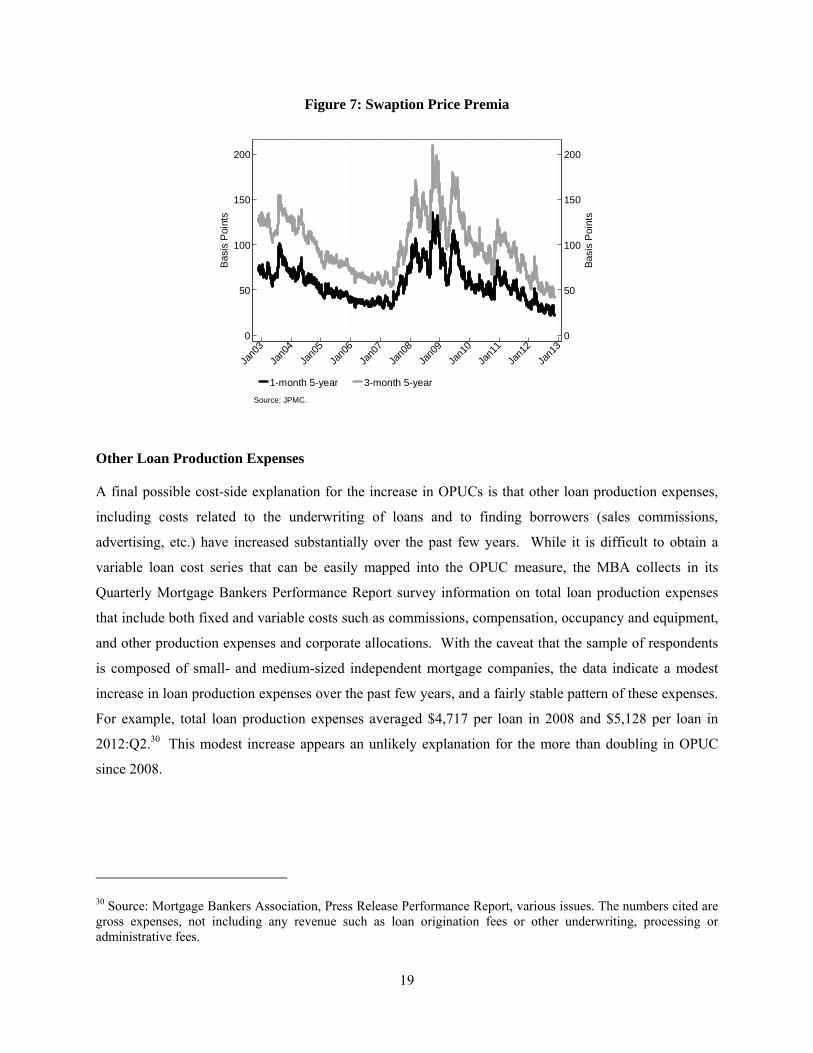
average about 30 percent and we assume that an originator hedges as much using swaptions. 29 Figure 7
shows the price premium in basis points for swaptions on a five-year swap rate with expiries of one and
three months. Conditional on a thirty-percent hedging strategy the cost of protection, when using a three-
month expiry, would be about 0.3 x 40 basis points = 12 basis points, or a 12 cents impact on OPUC. In
terms of the time-varying impact on OPUC, the extension in the length of the pipeline, which may have
lead originators to go from one-month to three-month expiry, also has a somewhat limited economic
impact on OPUC.
More generally and beyond our specific example, implied volatility and option price premia have
declined significantly since the fall of 2008, reflecting the lower rate volatility environment. While we do
not explicitly consider other more complex hedging strategies, the lower volatility environment has likely
also lowered the cost of these strategies. This is in contrast with the rise in OPUC over this period. In
sum, changing hedging costs do not appear to be able to account for a significant portion of the rise in
OPUC since 2008, and at least the cost of hedging fallout risk may in fact have declined during the
period.
29 For example, see pull-through numbers from the MBA’s Performance Report.
19
Figure 7: Swaption Price Premia
Other Loan Production Expenses
A final possible cost-side explanation for the increase in OPUCs is that other loan production expenses,
including costs related to the underwriting of loans and to finding borrowers (sales commissions,
advertising, etc.) have increased substantially over the past few years. While it is difficult to obtain a
variable loan cost series that can be easily mapped into the OPUC measure, the MBA collects in its
Quarterly Mortgage Bankers Performance Report survey information on total loan production expenses
that include both fixed and variable costs such as commissions, compensation, occupancy and equipment,
and other production expenses and corporate allocations. With the caveat that the sample of respondents
is composed of small- and medium-sized independent mortgage companies, the data indicate a modest
increase in loan production expenses over the past few years, and a fairly stable pattern of these expenses.
For example, total loan production expenses averaged $4,717 per loan in 2008 and $5,128 per loan in
2012:Q2.30 This modest increase appears an unlikely explanation for the more than doubling in OPUC
since 2008.
30 Source: Mortgage Bankers Association, Press Release Performance Report, various issues. The numbers cited are gross expenses, not including any revenue such as loan origination fees or other underwriting, processing or administrative fees.
0
50
100
150
200
Bas
is P
oint
s
0
50
100
150
200
Bas
is P
oint
s
Jan0
3
Jan0
4
Jan0
5
Jan0
6
Jan0
7
Jan0
8
Jan0
9
Jan1
0
Jan1
1
Jan1
2
Jan1
3
1-month 5-year 3-month 5-year
Source: JPMC.

20
4.2 Industrydynamicsandoriginators’profits
The discussion in the previous subsection appears to indicate that the higher OPUCs on regular agency-
securitized loans are not likely to be driven exclusively, or even mostly, by increases in costs. As a result,
the rise in OPUCs could reflect an increase in profits. If so, what are the potential driving forces behind
such an increase?
Capacity Constraints
An often-made argument is that there are significant capacity constraints in the mortgage origination
business these days, and that these capacity constraints become binding when the application volume
increases significantly, usually due to a refinancing wave. Originators then do not lower rates as much as
they would without capacity constraints, in order to curb the excess flow of applications.
Figure 8 provides some long-horizon evidence on the potential importance of capacity constraints for
profits, by plotting our OPUC measure against the MBA application index (including both purchase and
refinancing applications). The figure shows that the two series correlate quite strongly: whenever the
applications index goes up, OPUCs tend to go up, and vice-versa.31
This suggests that capacity constraints may play an important role in generating the higher OPUCs.
However, mortgage applications (and other measures of demand and origination activity, such as MBS
issuance) have been at higher levels in the past, without OPUCs being as high as they are now. Thus,
while simple capacity constraints that tend to arise in every refinancing wave can explain some of the
high-frequency variation in OPUCs, they appear to be an insufficient explanation as to why our baseline
OPUC measure has reached $5 now but not in the past.
31 Over the period 2004-08, the relationship between the two series appears weaker than elsewhere –OPUCs appear to be on a downward trend over much of that time, even when applications increase.

21
Figure 9 shows some more direct evidence on the potential importance of capacity constraints, by looking
at the number of days it takes from the initiation of a refinancing application to the funding of the loan.
The figure is based on data from the Home Mortgage Disclosure Act (HMDA), which is available only
through 2011, and from the Ellie Mae Origination Insight Report (EM), which is only available since
August 2011.32 It shows that the median (HMDA) or average (EM) number of days it takes for an
application to be processed and funded has been substantially higher since 2009 than it was in prior
years.33 The processing time moves in response to the MBA application volume shown earlier; for
instance, it reached its maximum after the refinancing wave of early 2009 and has increased from less
than 40 days in mid-2011 to above 55 days by October 2012 as refinancing has accelerated over this
period. However, to the extent that the HMDA and EM data are comparable, it does not appear that it
takes substantially longer to originate a refinancing loan now than it did in early 2009, making it difficult
to explain the rise in OPUC through capacity constraints.34
A final interesting question is how rigid capacity constrains may be. Current originators can add staff, but
it takes time to train new hires. New originators can enter the market, but entry requires federal and/or
32 http://www.elliemae.com/origination-insight-reports/EMOriginationInsightReportOctober2012.pdf
33 The average for HMDA would be higher than the median but would show similar patterns.
34 It is interesting to note that the time from refinancing application to funding was significantly lower in 2003, even though application volume was much higher than in recent times. This is likely driven by tighter underwriting now compared to the 2003 refinancing boom.
0
500
1000
1500
Inde
x le
vel
1
2
3
4
5
Do
llars
per
$1
00 lo
an
Jan9
4
Jan9
5
Jan9
6
Jan9
7
Jan9
8
Jan9
9
Jan0
0
Jan0
1
Jan0
2
Jan0
3
Jan0
4
Jan0
5
Jan0
6
Jan0
7
Jan0
8
Jan0
9
Jan1
0
Jan1
1
Jan1
2
Jan1
3
OPUCs MBA Market Volume Index (All applications)
Note: Two-month rolling window; Source: JPMC, Fannie Mae, MBA, authors calculations
Figure 8: Originator Profits and Unmeasured Costs and MBA Application Index

22
state licensing and approval from Fannie Mae, Freddie Mac and Ginnie Mae to fully participate in the
origination process. To the extent that training now may take longer than in the past, or that approval
delays for new entrants are longer (as anecdotally reported), the speed of capacity expansion may have
declined compared with earlier episodes.35
Figure 9: Time from Refinancing Application to Funding (by Month in which a Loan is Funded)
Market Concentration
A second popular explanation for the higher profits in the mortgage origination business is that the market
is highly concentrated. It is well-known that the mortgage market in the United States is dominated by a
relatively small number of large banks that originate the majority of loans. However, as shown in Figure
10, a simple measure of market concentration given by the share of loans made by the largest five or ten
originators has actually decreased over the period 2011-12, as a number of the large players have
decreased their market share (while the largest originator has further increased its origination share).
Thus, market concentration alone is unlikely to provide an explanation of high profits in the mortgage
business. This also makes sense from a theoretical point of view: there is no particular reason why a
concentrated market (but with a large number of fringe players) should incur large profits. A better
potential explanation for why originators would make larger profits now than in the past would be that
they may enjoy more pricing power than in the past on some of their borrowers.
35 Also, existing capacity may have been diverted to defending against put-backs instead of new loan origination.
10
20
30
40
50
60
# D
ays
Jan
2003
Jan
2004
Jan
2005
Jan
2006
Jan
2007
Jan
2008
Jan
2009
Jan
2010
Jan
2011
Jan
2012
HMDA (median) Ellie Mae (average)
Source: HMDA (Jan. 2003 - Dec. 2011); Ellie Mae (Aug. 2011 - Oct. 2012)Note: HMDA data restricted to first-lien mortgages for owner-occupants of 1-4 unit houses or condos.

23
Figure 10: Origination Market Concentration
HARP Refinance Loans
A market segment where such pricing power may be particularly important is the high-LTV segment,
which over the past years has been dominated by refinancings through HARP, originally introduced in
March 2009. The introduction of revised HARP rules in late 2011, often referred to as “HARP 2.0,” has
lead to a significant increase in HARP activity over the course of 2012; the FHFA estimates that in
August 2012 (the last month for which numbers have been reported), HARP refinancings accounted for
24 percent of total refinance volume. 36 HARP 2.0 provides significant incentives for same-servicer
refinancing (namely, relief from representations and warranties) which are not present for different-
servicer refinancings. As a consequence, many servicers do not offer HARP refinancing for loans that
they are not currently servicing, or only at much worse terms. The result is that the current servicer has
significant pricing power over its own high-LTV borrowers looking to refinance.
Is there evidence that lenders can exploit this higher pricing power? The observed note rates for HARP-
refinanced loans are at least consistent with this idea. As shown in Figure 11, the weighted average
coupons (WACs; that is, the loan rates) on HARP loans with LTVs above 105 tend to be 40-50 basis
points higher than those of regular refinancings or purchases. (HARP refinancings with LTVs between 80
and 105 have WACs about 25-40 basis points above those on regular refinancings/purchases.) Banks earn
higher revenues on HARP loans than on regular loans for two reasons: given the higher note rate, they
36 www.fhfa.gov/webfiles/24596/Aug-12_Refi_Report.pdf
20
40
60
80
Sha
re
2004
q1
2005
q1
2006
q1
2007
q1
2008
q1
2009
q1
2010
q1
2011
q1
2012
q1
2013
q1
Market share of top 10 lenders Top 5 Top 1
Source: Inside Mortgage Finance

24
will typically sell these loans into a pool with a 50 basis points higher note rate, which usually commands
a price premium around 1.5-2.0 points. Furthermore, thanks to the prepayment protection offered by these
pools (as a borrower can only refinance through HARP once), investors are willing to pay a higher price
(in the spec-pool market) than for TBA pools; this can add another 1-3 points (depending on the coupon)
to the originator’s revenue.
Figure 11: Weighted Average Coupons of Different Loan Types
Are these higher revenues compensation for higher origination costs for HARP loans? This seems
unlikely, as the documentation requirements for HARP loans are in fact significantly lighter than for
regular loans. Thus, it is likely that origination costs are lower, not higher, for HARP loans relative to
regular refinancings.37
Another possibility is that high LTV borrowers are more cash-constrained than regular refinancers and
thus require higher rebates (negative points) at origination to help cover their closing costs. While this is a
possibility, it is unlikely that the difference is so large as to take up a significant portion of the additional
revenues from above, especially since closing costs are likely lower than for regular loans (thanks e.g. to
37 Also, the loans with FICO scores of 720 or above that we include in the graph are not subject to loan-level price adjustments.
3.5
4
4.5
5
Jan 2012 Apr 2012 Jul 2012 Oct 2012
Purchase LTV<=80 Refi LTV<=80
Refi 105<LTV<=125 Refi LTV>125
Includes 30-year FRMs with loan amounts smaller than or equal to 417,000,made to borrowers with FICO score of at least 720, on owner-occupied 1-unit properties.Data source: Fannie Mae, Freddie Mac, eMBS.

25
appraisal waivers). Thus, the evidence strongly suggests that originators make larger profits on HARP
loans than on regular loans, by being able to exploit their pricing power.
Non-HARP Mortgages
The next question is whether similar pricing power could explain the part of the rise in our OPUCs on
regular (non-HARP) loans that seems left unexplained by capacity constraints, as discussed above. While
lenders may have pricing power over their HARP borrowers, it is much less clear whether such pricing
power may also exist for “regular” loans. Pricing power could arise for instance from customers’
impediments (actual or perceived) to shop around, an unwillingness of other firms to compete, barriers to
entry for new competitors, or a combination of these. Directly measuring originators’ pricing power is not
a trivial task, and we do not attempt a full analysis here. However, looking at some cross-sectional
patterns may suggest some insights at least.
Figure 11 shows that over 2012, the WAC on refinancing loans tends to be slightly larger than on
purchase loans. This is somewhat surprising if one thinks that the costs of originating a refinance loan are
likely lower than those of a purchase loan. However, the WAC divergence could be explained by
purchase borrowers paying more points than refinancers, for instance due to tax incentives.38
One would expect this explanation, if true to hold across all lenders. However, looking at lender-specific
differences in WACs reveals large variation across lenders. The two panels of Figure 12 show the
monthly average WAC for the sixteen largest lenders over 2012 (in terms of number of loans sold to the
GSEs), for purchase and refinancing loans separately. We also plot separately the average for all other
(smaller) sellers (the thicker lines). We only include thirty-year fixed-rate loans with FICO scores of 720
and higher and LTVs of 80 or lower made to single-unit owner-occupiers in order to reduce potential
disparities due to differential price adjustments.39
The top panel of the figure shows that purchase WACs across sellers are quite homogeneous --- with the
exception of a couple of outliers, most lender WACs lie within a range of approximately 10 basis points.
This is consistent with the idea that the purchase mortgage market is quite competitive, as presumably
many borrowers shop around.
38 See e.g., www.irs.gov/publications/p936/ar02.html#en_US_2011_publink1000229936
39 These calculations are based on the complete set of loan-level disclosures for pools issued in 2012 by Fannie Mae and Freddie Mac.

26
The bottom panel reveals a much larger dispersion for refinancing loans. In particular, while a number of
sellers remain concentrated around the thicker line representing the average of smaller players, eight of
these large lenders sell loans with WACs that are 20 basis points or more above the dashed line in at least
one month, and, for five of them that is the case for most months.40 In principle, this observed price
dispersion is certainly not inconsistent with the market being competitive; however, under this null
hypothesis it is surprising that the dispersion is so much larger for refinancing loans than for purchases.
As discussed above, over the course of 2012 the HARP program has gained significant momentum for
high-LTV refinances. A perhaps lesser-known fact is that there exist GSE streamline refinancing
programs also for non-HARP loans (with LTV less than 80), with the same cutoff date for eligible
mortgages (which must have been delivered to one of the GSEs prior to May 31, 2009). Streamlined
refinancing, when done through the institution that currently services the loan, relieves the lender from
representation and warranties relating to the borrower’s creditworthiness and home value, while a
different-servicer refinancing requires the new loan to be fully underwritten. As a consequence, for
borrowers eligible for a streamlined refinancing, there is an advantage to staying with the same
servicer/lender, as doing so will reduce the documentation the borrower will need to submit. This in turn
again creates some pricing power for the current servicer (although likely less so than for high-LTV
loans). The population of loans in fixed-rate GSE pools originated prior to June 2009 is large: as of
October 2012, almost $1.25 trillion of loans are in such pools, relative to an overall Fannie/Freddie fixed-
rate universe of about $3.75 trillion. During 2012, about 54 percent of all prepayments came from pools
issued prior to June 2009.41 Thus, if lenders have pricing power over the refinancings of these loans, this
could be a non-trivial contributor to OPUCs.
40 With the exception of one of these five lenders, the monthly number of sales of refinancing loans always exceeds 1,000 loans, meaning that these averages are unlikely to be driven by small-sample noise.
41 These prepayments include refinancings as well as the loan simply getting paid off (for instance due to the borrower moving).

27
Figure 12: Dispersion in Weighted Average Coupons across Sellers
A. Purchase Loans, Sales to Fannie Mae and Freddie Mac, 2012
B. Refinancing Loans, Sales to Fannie Mae and Freddie Mac, 2012
3.4
3.6
3.8
4
4.2
4.4
4.6
Jan 12 Apr 12 Jul 12 Oct 12
Average of smaller sellers
Includes loans with FICO of 720 or higher, LTV of 80 or lower, amount smaller than or equal to 417,000,on owner-occupied single-unit properties.Include only months in which a seller made at least 100 sales.Data source: Fannie Mae, Freddie Mac, eMBS.

28
Is there evidence that such pricing power could explain the dispersion in refinancing WACs?
Unfortunately, unlike for HARP loans, there is no way for us to observe in the data whether a refinancing
was streamlined or not. However, we can look at variation across lenders in the fraction of their servicing
portfolio that could potentially be refinanced in a streamlined manner (that is, loans in pools issued prior
to June 2009), and correlate this with the average WAC of the lenders’ non-HARP refinance loans over
2012. Figure 13 shows that there is indeed a positive correlation between the two: the lenders that had a
large fraction of potentially streamline-eligible loans in their servicing portfolio at the end of 2011 tend to
be those that originate refinance loans with the highest WACs on average over 2012 (that is, those that are
above the thick line in Panel B of Figure 12). This is consistent with (though certainly not proof of)
originators taking advantage of their pricing power over streamline-eligible borrowers.
Figure 13: WACs on regular (low LTV) refinance loans correlate with fraction of servicers’ portfolio eligible for streamline refinancing
Notes: HARP- or streamline-eligible pools = pools issued prior to June 2009. Only includes sellers/servicers with servicing portfolio with >$1bn of HARP- or streamline-eligible pools in November 2011. Non-HARP WACs calculated on loans with FICO of 720 or higher, LTV of 80 or lower, amount smaller than or equal to 417,000, on owner-occupied single-unit properties. Data sources: Fannie Mae, Freddie Mac, eMBS.
-.2
0
.2
.4
WA
Cs
of n
on-
HA
RP
re
fis r
elat
ive
to s
mal
ler
selle
rs o
ver
201
2 (a
vg. a
cro
ss m
onth
s)
.3 .4 .5 .6 .7Share of Nov 2011 servicing portfolio in HARP- or streamline-eligible pools

29
5. Conclusions
The increasing gap between primary and secondary mortgage rates over the past few years has been
reflected in a rise in OPUCs, originators’ profits and unmeasured costs. The magnitude of the OPUCs are
influenced by MBS prices, the valuation of servicing rights, points paid by borrowers, as well as costs
such as g-fees, putback risks and “pipeline” hedging.
The rise in OPUCs is mainly driven by higher MBS prices, which are not offset by corresponding
increases in measurable costs. Conversely, a decline in the value of mortgage servicing rights may have
reduced OPUCs to some extent, and thus contributed to the widening primary-secondary spread. Among
harder-to-measure costs, we find that putback risk and pipeline hedging likely cannot explain the full rise
in OPUCs. Absent other cost increases that we cannot measure well, such as operating costs, the rise in
OPUCs reflects to some extent an increase in originator profits. While market concentration alone does
not seem to explain the rise in these profits, capacity constraints do appear to play a significant role.
Additionally, we provide evidence suggesting that originators have enjoyed pricing power on some of
their borrowers looking to refinance over the past year.
Going forward, it will be important to monitor the extent to which capacity expansions, new entry,
changes in regulations, and (in the longer term) housing finance reform will affect the pass-through from
secondary to primary markets. As illustrated in this paper, a number of factors potentially affect this pass-
through, and it is important for policy makers and market participants to further improve the measurement
and understanding of these factors.

30
Appendix A: Detail on Coupon Selection and OPUC Calculation
The following table provides more detail on the “best execution” calculation, which is run at a weekly frequency to compute the OPUC series. Basic inputs are the average mortgage rate and points paid by borrowers, the effective g-fee, as well as TBA prices (sources are given below).
Taking the mortgage rate and points as given, we consider three different TBA coupons into which the mortgage could potentially be pooled. The highest coupon is set such that it requires the originator to buy down the g-fee upfront, while this is not the case for the other two possible coupons (where the originator retains positive excess servicing because the loan’s interest payment is more than sufficient to cover the g-fee and base servicing). Depending on the mortgage rate, pooling into the highest coupon may not actually be a possibility – as mentioned in the main text, the mortgage rate needs to exceed the coupon rate by at least 25 basis points. In the example in the table below, pooling a mortgage with note rate 4.6 into a 4.5 coupon is not feasible, but the column is nevertheless included in the example to show the mechanics of the g-fee buydown.
As shown in the table, the main trade-off between pooling into the 4.0 or the 3.5 coupon lies in the cash obtained from the sale of the security (which is larger for the high coupon) versus the higher value of excess servicing if the lower coupon is chosen. Which coupon is preferable thus depends on the coupon swap (i.e. the price difference between the two coupons) and the assumed value of excess servicing.42
42 If the highest coupon is feasible, it also depends on the buydown multiple.
Date: 7/7/2011TBA coupon (%) 3.5 4 4.5 (1)
Coupon-independent inputs (%)Mortgage rate (2)
Points (3)G-fee (4)
Base servicing (5)Excess servicing 0.539 0.039 -0.461 (6) = (2) - (1) - (4) - (5)
Coupon-specific inputs ($ per par value)TBA price (back month) 95.78 100.08 103.51 (7)Value of base servicing 1.25 1.25 1.25 (10) = 5 * (5)Value of excess servicing 2.16 0.16 (11) = 4 * (6) if (6) > 0G-fee buydown -3.23 (12) = 7 * (6) if (6) < 0
Revenues from TBA sale less payout to borrower -3.52 0.78 4.21 (13) = (7) - 100* (1 - (3) / 100)Value of servicing net of g-fee 3.41 1.41 -1.98 (14) = (10) + (11) + (12)
OPUCBy coupon -0.11 2.18 2.23 (15) = (13)+(14)Best execution 2.18 (16) = max(15) if (2) - (1) > .25
4.60.7
0.3110.25
31
The example in the table (and the calculations in the main text) assume, counterfactually, that the g-fee is only a flow payment. In practice, there are also upfront surcharges that need to be paid to the GSEs upon delivery, known as loan-level price adjustments (LLPAs) in case of Fannie Mae, and postsettlement delivery fees in case of Freddie Mac. These contain a fixed charge for all loans (currently 25 basis points) known as adverse-market delivery charge (AMDC), as well as loan-specific additional charges, depending for instance on the term of the loan and the borrower’s FICO and LTV.43 For instance, at the time of this writing the LLPA for a borrower with a FICO score of 730 and an LTV of 80 would be 50 basis points (for a 30-year fixed-rate loan; the charge is waived for loans with term 15 years or less). Together with the AMDC, this would mean that an additional 0.75 would be subtracted from line (13) in the table. In our calculations, instead, it is assumed that this charge is paid over the life of the loan, because this is how Fannie Mae reports effective g-fees in their 10-Q filings. Additional notes and data sources: Mortgage rate and points: Values obtained from the Freddie Mac Primary Mortgage Market Survey (U.S. average). G-fee: Monthly interpolated series from Fannie Mae 10-Q filings. This reported g-fee includes both the component collected out of interest payments on a monthly basis and the upfront charges discussed above, transformed into a flow value based on estimated average life of the loans. Base and excess servicing: Base servicing is always 25 basis points. Excess servicing is the difference between the mortgage rate and the sum of g-fee, coupon payment and base servicing. TBA price: For each coupon is the Fannie Mae 30y FRM TBA back-month contract price. Source: JPMC. Servicing Values: Dollar value of the servicing streams obtained by multiplying the respective yearly flows by a base (5x) and an excess (4x) multiple. G-fee buydown: When excess servicing is negative as in the case of the 4.5 coupon in the table, the payment from the borrower is insufficient to cover the coupon payments, g-fee and base servicing. In this case the loan can be securitized into the coupon upon an upfront payment to the GSE equal to the dollar value of the missing flow (valued at a multiple of 7x). In the example above the excess servicing is larger than the g-fee in absolute magnitude, meaning that the mortgage rate is insufficient to cover the coupon payment and base servicing. Based on GSE policies the loan cannot be securitized in this coupon. Revenues from TBA sale less borrower payout: The payout is equal to par less points paid by the borrower. Value of servicing net of g-fee: Sum of all servicing streams net of the g-fee OPUC by coupon: Sum of revenues from TBA sale and servicing net of g-fees and borrower’s payout Best execution: Highest OPUC across coupons conditional on the mortgage rate being at least 25 basis points above the coupon rate in order to cover base servicing. In this case the loan cannot be securitized in the 4.5 coupon, the optimal execution is to securitize the loan in the 4.0 coupon.
43 The list of price adjustments for Fannie Mae and Freddie Mac can be found at www.fanniemae.com/content/pricing/llpa-matrix.pdf and www.freddiemac.com/singlefamily/pdf/ex19.pdf.


