Embed Size (px)
Citation preview

IZA DP No. 3712
The Rise and Fall of Spanish Unemployment:A Chain Reaction Theory Perspective
Marika KaranassouHector Sala
DI
SC
US
SI
ON
PA
PE
R S
ER
IE
S
Forschungsinstitutzur Zukunft der ArbeitInstitute for the Studyof Labor
September 2008

The Rise and Fall of
Spanish Unemployment: A Chain Reaction Theory Perspective
Marika Karanassou Queen Mary, University of London
and IZA
Hector Sala Universitat Autònoma de Barcelona
and IZA
Discussion Paper No. 3712 September 2008
IZA
P.O. Box 7240 53072 Bonn
Germany
Phone: +49-228-3894-0 Fax: +49-228-3894-180
E-mail: [email protected]
Any opinions expressed here are those of the author(s) and not those of IZA. Research published in this series may include views on policy, but the institute itself takes no institutional policy positions. The Institute for the Study of Labor (IZA) in Bonn is a local and virtual international research center and a place of communication between science, politics and business. IZA is an independent nonprofit organization supported by Deutsche Post World Net. The center is associated with the University of Bonn and offers a stimulating research environment through its international network, workshops and conferences, data service, project support, research visits and doctoral program. IZA engages in (i) original and internationally competitive research in all fields of labor economics, (ii) development of policy concepts, and (iii) dissemination of research results and concepts to the interested public. IZA Discussion Papers often represent preliminary work and are circulated to encourage discussion. Citation of such a paper should account for its provisional character. A revised version may be available directly from the author.

IZA Discussion Paper No. 3712 September 2008
ABSTRACT
The Rise and Fall of Spanish Unemployment: A Chain Reaction Theory Perspective*
The evolution of Spanish unemployment has been quite idiosyncratic. The full employment levels of the early seventies were followed by unemployment rates that were the highest within the OECD countries in the aftermath of the oil price shocks. While unemployment was extremely persistent in most of the eighties and nineties, it experienced its sharpest decline in recent years. We investigate the determinants of this unemployment trajectory using the analytical framework of the chain reaction theory (CRT). We show that unemployment may not gravitate towards its natural rate due to frictional growth, a phenomenon that arises from the interplay of lagged adjustment processes and growing exogenous variables in a dynamic system with spillovers. The empirical analysis distinguishes four periods: (i) 1978–1985, (ii) 1986–1990, (iii) 1991–1994, (iv) 1995–2005, and finds that capital accumulation is a crucial driving force of unemployment. Thus, our theoretical and empirical results question the key role of the natural rate in policy making. JEL Classification: E22, E24, J21 Keywords: labour market dynamics, frictional growth, chain reaction theory,
capital accumulation, impulse response function Corresponding author: Hector Sala Departament d’Economia Aplicada Universitat Autònoma de Barcelona 08193 Bellaterra Spain E-mail: [email protected]
* Hector Sala is grateful to the Spanish Ministry of Education and Science for financial support through grant SEJ2006-14849/ECON.
1 Introduction
The evolution of Spanish unemployment over the past thirty five years has been unique
among the OECD countries. The full-employment levels of the early seventies were, sur-
prisingly, followed by the highest unemployment rates in the aftermath of the oil price
shocks, and the most persistent unemployment problem in the eighties and nineties. The
size and duration of high unemployment rates, in the range of around 10%-20% for approx-
imately 20 years, have been dubbed the "Spanish disease" (Dolado and Jimeno, 1997).
And somehow, Spain has again surprised by its rapid and prolonged unemployment rate
decline over the second half of the nineties (the fall in unemployment of around 10 per-
centage points was the sharpest in the OECD area).
Figure 1 plots the unemployment rate trajectory by distinguishing four periods: (i)
1978-1985, (ii) 1986-1990, (iii) 1991-1994, and (iv) 1995-2005.1 Bentolila and Jimeno
(2006) refer to the first one as the ‘long recession’, the next two as the ‘EU cycle’, and
the last one as the ‘EMU cycle’.
Figure 1. Unemployment rate
0
4
8
12
16
20
24
1970 1975 1980 1985 1990 1995 2000 2005
%"longrecession" "EU cycle"
"EMU cycle"
The consensus view is that a combination of labour unfriendly institutions (e.g. bene-
fits) and adverse macroeconomic shocks (e.g. oil crises) were responsible for the develop-
ment of the so-called "Spanish disease". Although the "usual suspects" such as wage-push
1Some studies use the Spanish labour market figures provided by the quarterly Survey of the ActivePopulation (Encuesta de Población Activa, EPA), which underwent methodological changes in 1987,1992, 2002, and 2005 (see Garrido and Toharia, 2004). Here we use the homogeneous long-time seriesprovided by the OECD Economic Outlook, which slightly deviate from the EPA series.
2

factors, taxes and stock-market swings do matter, we argue that the crucial driving force
of unemployment is capital accumulation.
The conventional wisdom for the rise and fall of Spanish unemployment has evolved
along the lines of the natural rate of unemployment, NRU (or NAIRU)2 story using a
variety of methodologies. The econometric models include multi-equations à la Layard,
Nickell and Jackman (1991), single-equations à la Phelps (1994), structural vector au-
toregressions (VARs), and the observable shocks model of Blanchard and Wolfers (2000).
Dolado, Malo de Molina and Zabalza (1986), using a structural multi-equation model,
argue that the policies most suited to reducing unemployment without increasing inflation
are lower taxation, a higher degree of labour market flexibility, and more effective incomes
policies. Phelps and Zoega (2001) estimate a single-equation model for a panel of OECD
countries and find that the long swings in economic activity result from the changes in
expected future productivity, which can be proxied by the swings in the stock market.
Spain appears as the most sensitive economy to these swings, although the omission of
country-specific variables is acknowledged. Dolado and Jimeno (1997), using a structural
VAR methodology, attribute the dismal performance of Spanish unemployment to a series
of adverse shocks -‘price shocks in the late 70s, wage shocks in the early 80s, and demand
shocks in the early 90s’ (p. 1285)- which were amplified by a rigid system of labour market
institutions (e.g. collective bargaining, high firing costs, and barriers to competition in
the goods market). Bentolila and Jimeno (2006), using the Blanchard and Wolfers (2000)
model of equilibrium unemployment in the OECD, argue that Spain is characterised by a
set of ‘strongly unemployment generating’ labour market institutions (i.e. unemployment
benefits, employment protection, and collective bargaining) which aggravate the effects of
adverse macroeconomic shocks.
In contrast to the above literature, this paper examines the Spanish labour market
from the perspective of the CRT (chain reaction theory). The CRT uses dynamic struc-
tural multi-equation systems and postulates that the unemployment rate is driven by the
interplay between interacting lagged adjustment processes and spillover effects. Spillovers
arise when shocks to a specific equation feed through the labour market system, where
"shocks" refer to changes in the exogenous variables.
The importance of having distinct equations for labour force and employment in the
labour market model, rather than compressing them into a single-equation unemployment
rate model, becomes evident from Figure 2. The disparity between the time paths of
labour force and employment indicates that aggregating them into a single unemployment
2Tobin (1998) argues that the NAIRU (non accelerating inflation rate of unemployment) and NRUare not synonymous. However, within our context of analysis, such a distinction is superfluous. SeeKaranassou, Sala and Snower (2008) for a survey and critique of NAIRU and NRU models.
3

rate equation will produce a biased summary of their evolution.3 According to Figure 2,
labour force did not grow much in the seventies and early eighties. Although there was
an acceleration in the second half of the eighties, it is since the mid nineties that this
growth has been the fastest. On the other hand, employment figures show a much more
procyclical behaviour.
Figure 2. Employment, unemployment, and labour force
10
11
12
13
14
15
16
17
18
19
20
21
22
1970 1972 1974 1976 1978 1980 1982 1984 1986 1988 1990 1992 1994 1996 1998 2000 2002 2004 2006
Employment
Labour force
Unemployment
Note: Employment, unemployment and labour force expressed in millions.
Generally, a CRT labour market model comprises labour demand, labour supply and
wage setting equations. The system is dynamic due to the existence of adjustment costs
which are well known in the literature. There are employment adjustment costs due to
labour turnover costs, such as the costs of hiring and firing workers; wage setting costs due
to nominal wage and price staggering; and labour force adjustment costs, due to monetary
and psychic costs of entering and exiting the labour force. Spillovers are created when
endogenous variables appear as explanatory variables in other equations (for example,
wages in the labour demand and labour force equations, or the unemployment rate in the
wage setting equation).
Each shock generates an intertemporal chain reaction of effects capturing the interplay
between the dynamics and the spillovers of the system. These chain reactions are described
in terms of impulse response functions. Therefore, the CRT represents a synthesis of
traditional structural macroeconometric models and structural VARs.
Another important feature of the CRT is that it allows trended variables, such as
capital stock, working-age population, or capital deepening, to influence unemployment.
Unlike the NRU models, which impose strong a-priori restrictions, the CRT ensures that
each equation is balanced (dynamically stable), so that each trended dependent variable
3For a comparison between multi-equation and single-equation unemployment rate approaches, seeKaranassou, Sala and Snower (2003).
4

is driven by the set of its trended determinants. This distinguishes the CRT from the-
ories that just consider stationary variables as potential determinants of the trendless
unemployment rate.
Finally, the interplay of lags (due to adjustment costs in labour market activities)
and growing variables (due to the trended nature of the dependent variables) gives rise
to the phenomenon of frictional growth. In the presence of frictional growth (FG), as we
show in Section 2, long-run unemployment equals its NRU plus FG, and, consequently,
unemployment cannot be decomposed into "trend" and cyclical components. In other
words, since actual unemployment does not gravitate towards its natural rate, frictional
growth challenges the central role attached by the mainstream theories to the NRU for
explaining the rise and fall of unemployment.
Our empirical analysis of labour market dynamics shows that the growth rate of capital
stock plays a crucial role in shaping unemployment movements during all the four periods
portrayed in Figure 1. Although benefits, taxes, and financial wealth do influence unem-
ployment, capital accumulation is the most substantial contributor to the unemployment
trajectory.
The remaining of the paper is structured as follows. Section 2 analyses a stylised
labour market model to convey the central features of the CRT. Section 3 provides a
comprehensive overview of the Spanish experience in last decades. Section 4 is concerned
with the econometric methodology and the estimated labour market system. The empiri-
cal model is used in Sections 5 and 6 to measure, respectively, the dynamic contributions
of the exogenous variables to the evolution of unemployment, and the long-run impact of
capital accumulation on the unemployment trajectory. Section 7 concludes.
2 Chain Reaction Theory (CRT)
To understand the development of the unemployment problem, the chain reaction theory
advocates the use of interactive dynamic labour market models, i.e. dynamic multi-
equation systems with spillover effects. Spillovers arise when endogenous variables have
explanatory power in other equations of the system. By chain reactions we refer to the
intertemporal responses of the unemployment rate to changes in the exogenous variables
("shocks"). The chain reactions are generated by the interplay between the dynamics and
spillovers of the system. The analytical model below illustrates the workings of the CRT
and is in line with our estimated labour market model in Section 5.
5

2.1 A Stylised Labour Market Model
Consider the following labour demand, real wage, and labour supply equations:4
nt = α1nt−1 + β1kt − γ1wt, (1)
wt = α2wt−1 + β2xt − γ2ut, (2)
lt = β3zt + γ3wt, (3)
and let the unemployment rate be defined as5
ut = lt − nt, (4)
where ut is the unemployment rate; nt, wt, and lt denote employment, real wage, and
labour force, respectively; kt is real capital stock, xt represents a wage-push factor, and
zt is working-age population; the β’s, and γ’s are positive constants. All variables, except
the unemployment rate, are in logs and the error terms are ignored for expositional ease.
The autoregressive parameters α1 and α2 are positive and less than unity, capturing the
employment adjustment and wage/price staggering effects, respectively. Generally, we
refer to the lags of the endogenous variables in a CRT model as the "lagged adjustment
processes".
It is important to note that, unlike the single-equation NRU models, the CRT models
may also include trended exogenous variables. The only requirement is that each equation
is balanced (i.e. dynamically stable) so that each trended dependent variable is driven
by the set of its trended determinants. It can be shown that equilibrating mechanisms in
the labour market and other markets jointly act to ensure that the unemployment rate is
trendless in the long-run (Karanassou and Snower, 2004). In terms of the above analytical
model, these mechanisms can be expressed in the form of restrictions on the relationships
between the long-run growth rates of the growing exogenous variables (see Section 2.4).
The γ’s generate spillover effects, since changes in an exogenous variable in one equa-
tion, say capital stock in labour demand, can also affect the real wage and labour supply
equations. Observe that if the wage elasticities are zero (γ1 = γ3 = 0) , the wage-push
factor (xt) does not influence unemployment. In addition, if unemployment does not
put downward pressure on wages (γ2 = 0), changes in capital stock (kt) and working-age
population (zt) do not spillover in the labour market system and so their unemployment
effects can be adequately captured by the labour demand (1) and supply (3) equations.6
4It can be shown that the above labour market model is compatible with standard microeconomicfoundations.
5Since labour force and employment are in logs, the unemployment rate can be approximated by theirdifference.
6This is because labour demand and labour supply are linked via wages. If changes in the capital stock
6

Therefore, in the presence of spillover effects, the individual labour demand and supply
equations cannot provide adequate measures of the sensitivities of unemployment to the
exogenous variables. We refer to the β’s as the "local" short-run elasticities in order to
distinguish them from the "global" ones, which incorporate all the feedback mechanisms
in the labour market model. The global elasticities can be obtained by the univariate
representation of unemployment which we derive below.7
2.2 Univariate Representation of Unemployment
Rewrite the demand, wage, and supply equations (1)-(3) as
(1− α1B) (1− α2B)nt = β1 (1− α2B) kt − γ1 (1− α2B)wt, (5)
(1− α2B)wt = β2xt − γ2ut, (6)
(1− α1B) (1− α2B) lt = β3 (1− α1B) (1− α2B) zt + (7)
γ3 (1− α1B) (1− α2B)wt,
where B is the backshift operator, and substitute (6) into (5) and (7) to obtain the
following equations for employment and labour force:
(1− α1B) (1− α2B)nt = β1 (1− α2B) kt − γ1β2xt + γ1γ2ut, (8)
(1− α1B) (1− α2B) lt = β3 (1− α1B) (1− α2B) zt + (9)
γ3β2 (1− α1B)xt − γ3γ2 (1− α1B)ut,
respectively.
The univariate representation (or reduced form dynamics) of the unemployment rate
can be obtained by inserting the above equations into (4):8
[(1− α1B) (1− α2B) + γ3γ2 (1− α1B) + γ1γ2]ut = −β1 (1− α2B) kt (10)
+γ3β2 (1− α1B)xt + γ1β2xt
β3 (1− α1B) (1− α2B) zt.
The term "reduced form" relates to the fact that the parameters of the equation are not
estimated directly, instead, they are some nonlinear function of the parameters of the
and working-age population do not influence wages (γ2 = 0) they cannot spillover to the system. Theindividual labour demand and supply equations can sufficiently capture their effects on unemployment.
7The univariate representation expresses unemployment as a function of it own lags and the exogenousvariables in the system.
8Note that (10) is dynamically stable since (i) products of polynomials in B which satisfy the stabilityconditions are stable, and (ii) linear combinations of dynamically stable polynomials in B are also stable.
7

underlying labour market system (1)-(3).
We can reparameterise the above equation as
ut = φ1ut−1 − φ2ut−2 − θkkt + θx (γ1 + γ2)xt + θzzt + (11)
α2θkkt−1 − α1γ3θxxt−1 − (α1 + α2) θzzt−1 + α1α2θzzt−2,
where φ1 =α1+α2+α1γ2γ31+γ1γ2+γ2γ3
, φ2 =α1α2
1+γ1γ2+γ2γ3, θk =
β11+γ1γ2+γ2γ3
, θx =β2
1+γ1γ2+γ2γ3, and
θz =β3
1+γ1γ2+γ2γ3.
The univariate representation (11) shows that unemployment is generated by the in-
terplay of lagged adjustment processes and spillovers. In particular, the autoregressive
coefficients φ1 and φ2 embody the interactions of the employment adjustment (α1) and
wage-price staggering (α2) processes. The θ’s embody the feedback mechanisms built
in the system, since they are a function of the semi-elasticities (β’s) of the individual
equations (1)-(3) and the spillovers (γ’s). Thus, the θ’s describe the "global" short-run
sensitivities of unemployment with respect to the exogenous variables. The interplay of
dynamics across equations is further emphasized by the lagged structure of the exoge-
nous variables. Using time series jargon, we refer to the lagged exogenous variables as
"moving-average" terms.
Another key element of the CRT is that capital stock, a trended variable, influences
the time path of the unemployment rate, a stationary variable. We can justify this result
as follows. Capital stock initially enters the system as a determinant of employment,
a trended variable. Labour demand (1) is a balanced equation since it is dynamically
stable (|α1| < 1) . Similarly, the trended labour force is driven by working-age population(also a trended variable), and the static labour supply (3) is itself a balanced equation.
According to (8)-(9), the labour demand and supply equations remain balanced once the
wage (2) has been substituted into them.9
2.3 Impulse Response Functions
The responses of unemployment through time (Rt+j, j ≥ 0) to a one-off unit shock (im-pulse), occurring at period t, are described by the impulse response function (IRF) of its
univariate representation (11). Unemployment persistence (σ) can be defined as the sum
of its future responses, i.e. for all periods in the aftermath of the shock:10 σ ≡P∞
j=1Rt+j.
Note that the responses can be interpretted as the "global" elasticities (strictly speak-
ing, semi-elasticities or slopes) of the unemployment rate, since shocks in the CRT refer
9Note that (8) and (9) are dynamically stable since the products of polynomials in B which satisfythe stability conditions are also stable.10Other measures of persistence are the half life of the shock, the sum of the autoregressive parameters,
and the largest autoregressive root.
8

to changes in the exogenous variables. In particular, the contemporaneous response (Rt)
captures the "global" short-run elasticity, whereas the sum of all responses measures the
"global" long-run elasticity. In other words, the short-run elasticity plus persistence equals
the long-run elasticity of the specific variable:
long-run elasticityP∞j=0Rt+j
= short-run elasticity
Rt
+ persistenceP∞j=1Rt+j
(12)
Furthermore, we can measure the contributions of an exogenous variable, say x, to
the evolution of unemployment over a specific period of time , say t = 0 to t = T , by
sequentially adding up the IRFs of the respective changes during the specific period. Let
∆xj = xj − xj−1, where j = 1, 2, ...T , and ∆ is the first difference operator. The IRFs of
these T shocks are:
t = 1 t = 2 ... t = T
IRF1 : R11 R12 ... R1T
IRF2 : − R22 ... R2T
... − − ... ...
IRFT : − − ... RTT
where IRFj denotes the response function to the jth shock, and Rjt is the response to
shock j in time t. Note that the diagonal elements denote the respective contemporaneous
responses to the various shocks.
We measure the t-period contribution as the sum of all responses at this period. There-
fore, the contributions of the exogenous variable x to the unemployment trajectory for
the given interval are given by the following time series:
t = 1 t = 2 t = 3 ... t = T
R11,2P
j=1
Rj2,3P
j=1
Rj3, ...TPj=1
RjT .(13)
An important drawback of the traditional structural macroeconometric models is that
the IRFs are missing from their analysis. This is because the plethora of spillover effects
in the system can substantially affect the size and sign of the "local" elasticities so that
the individual equations can be quite misleading regarding the effects of the exogenous
variables on unemployment. By focusing on the IRFs of the system, (structural) VARs
offer a statistically robust alternative. Unlike the traditional macroeconometric models,
the CRT emphasizes the role of IRFs in its investigation and uses the global elasticities as
a misspecification tool to diagnose the economic plausibility of the model. Thus, the CRT
methodology can be viewed as a synthesis of the traditional structural macroeconometric
9
models and the (structural) VARs.
2.4 Frictional Growth
In what follows, we show that in the CRT framework of analysis unemployment may
substantially deviate in both the short- and long-run from what is commonly perceived as
its natural rate. This was first pointed out by Karanassou and Snower (1997) and opposes
the conventional wisdom that the NRU is the attractor of the unemployment rate.
We demonstrate this result by making the plausible assumption that capital stock (kt)
and working age population (zt) are growing variables with growth rates that stabilise
in the long-run. We also assume, for simplicity and without loss of generality, that the
wage-push factor (xt) does not grow in the long-run. Note that the growth rates of log
variables are proxied by their first differences, ∆ (·), and the superscript LR denotes the
long-run value of the variable.
The unemployment definition (4) implies that the unemployment rate stabilises in the
long-run, ∆uLR = 0, if the growth rate of employment is equal to the growth rate of
labour force, say λ,
∆lLR = ∆nLR = λ. (14)
The above restriction can also be expressed in terms of the long-run growth rates of the
exogenous variables:β1
1− α1∆kLR = ∆zLR. (15)
We refer to (15) as the frictional growth (FG) stability condition, since it ensures that the
unemployment rate stabilises in the long-run.
Let us reparameterise the demand (1) and wage equations (2) as
nt =β1
1− α1kt −
γ11− α1
wt −α1
(1− α1)∆nt, (16)
wt =β2
1− α2xt −
γ21− α2
ut −α2
(1− α2)∆wt, (17)
respectively. Next, substitute the wage eq. (17) into the demand (16) and supply equa-
tions (3):
nt =β1
1− α1kt −
γ1β2(1− α1) (1− α2)
xt +γ1γ2
(1− α1) (1− α2)ut
+γ1α2
(1− α1) (1− α2)∆wt −
α1(1− α1)
∆nt, (18)
lt = β3zt +γ3β21− α2
xt −γ3γ21− α2
ut −γ3α21− α2
∆wt (19)
10

Substitution of the above equations into (4) and some algebraic manipulation yields
the following expression for the unemployment rate:
ut =1
ζ
∙β3zt −
β11− α1
kt +(1− α1) γ3β2 + γ1β2(1− α1) (1− α2)
xt
¸+1
ζ
∙α1
(1− α1)∆nt −
(1− α1) γ3α2 + γ1α2(1− α1) (1− α2)
∆wt
¸,
(20)
where ζ =³1 + γ1γ2
(1−α1)(1−α2) −γ3γ21−α2
´.
The above leads to the following unemployment rate equation in the long-run:
uLR =1
ζ
⎡⎢⎢⎢⎣µβ3z
LR − β11− α1
kLR +(1− α1) γ3β2 + γ1β2(1− α1) (1− α2)
xLR
| {z }natural rate of unemployment
+α1β1
(1− α1)2∆kLR| {z }
frictional growth
⎤⎥⎥⎥⎦ , (21)
since ∆nLR = β11−α1∆kLR and ∆wLR = 0. The first term of (21) gives the NRU, whereas
the second term of (21) captures frictional growth. Note that when the exogenous variables
have nonzero long-run growth rates, unemployment is trendless in the long-run under the
FG stability condition (15).
According to (20), if the growth rate of employment is zero in the long-run¡∆nLR = 0
¢,
the first term of (20) in square brackets is the "trend" component of unemployment, while
the second term in square brackets is its cyclical component (since it is zero in the long-
run). However, under frictional growth, this decomposition cannot be obtained. This
distinguishes the CRT from models which filter out the cyclical variations of unemploy-
ment (e.g. using 5-year averages) and then identify its driving forces.
The long-run value¡uLR
¢towards which the unemployment rate converges reduces to
the NRU only when frictional growth is zero. In the above CRT model this occurs if (i)
the long-run growth rate of capital stock is zero or (ii) the lagged adjustment effect is
zero (α1 = 0). Therefore, frictional growth implies that under quite plausible conditions
the natural rate is not an attractor of the moving unemployment, and so the relevance of
the NRU in policy making is questionable.11 Reliance on natural rate estimates without
taking into account the impact of FG may, for example, lead to a misjudgment of the
unemployment effects of labour market reforms.
2.5 Long-run, Natural Rate, Contributions
To sum up, the interplay between lagged adjustment processes and growing exogenous
variables generates frictional growth, which has the following implications.
11For example, Karanassou and Sala (2008a) find that the NRU explains only 33% of the unemploymentvariation in Denmark, while frictional growth accounts for the remaining 67%.
11

• The NRU is not a reference point for the actual unemployment rate:
long-run = NRU
(steady-state)
+ frictional growth
• Unemployment cannot be decomposed into "trend" and cyclical components. Thisis in contrast with the standard NRU models:12
ut = αut−1 + βxt or ut =β
1− αxt| {z }
"trend" or NRU
− α
1− α∆ut| {z }
cyclical
,
since, by construction ∆uLR = 0.
• Since the unemployment rate is trendless, NRUmodels assert that growing variablescan only influence the labour market via their trendless transformations. Unlike
NRU models, the CRT models may also include trended exogenous variables. The
only requirement is that each equation is balanced (i.e. dynamically stable) so that
each trended dependent variable is driven by the set of its trended determinants.
Consequently, the univariate representation of unemployment is itself balanced and
the frictional growth stability condition (14) ensures that the unemployment rate
stabilises in the long-run
As we argued above, there may be a substantial disparity between the long-run and
natural rates of unemployment due to frictional growth. Our limited knowledge of the
long-run values of the growth rates of the exogenous variables implies that we do not have
reliable estimates of frictional growth, and consequently of the long-run unemployment
rate.
Thus, CRT models do not attempt to determine the factors underlying the natural (or
long-run) unemployment rate. Instead, the focus is on the contributions of the exogenous
variables to the evolution of the unemployment rate, which were defined by equation (13).
2.6 CRT, NRU, and Hysteresis
In what follows we briefly compare and contrast the chain reaction, natural rate, and
hysteresis theories of unemployment.13
• The short-run (cyclical) and long-run (natural) unemployment rates are12The AR(1) model is used for expositional ease.13See Karanassou, Sala, and Snower (2008) for a comprehensive survey and critique of the NRU and
hysteresis theories.
12

— interdependent in CRT models
— compartmentalised in NRU and hysteresis models.
• The effects of temporary shocks on unemployment
— dissipate through time in CRT and NRU models
— propagate to its natural rate in hysteresis models.
• While CRT and NRU models can identify the driving forces of the unemploymentrate, hysteresis models simply offer statistical representations of its trajectory.
• Whereas CRT estimates a labour market system and then derives the univariate
representation of the unemployment rate, NRU single-equation models estimate a
reduced-form unemployment rate equation.
It is worthwhile pointing out that linearity is the common ground for all three theories,
i.e. the unemployment rate process in NRU, hysteresis, and CRT models responds to
shocks in a linear fashion. The hysteresis theory in the above discussion refers only to the
popular "unit root hysteresis". It is beyond the scope of this paper to discuss hysteretic
models which display remanence, i.e. positive and negative shocks of equal size do not
cancel out. This type of hysteresis involves economic models with heterogeneous agents
who respond nonlinearly to shocks (Cross et al., 1999).
3 Overview of the Spanish experience
Spain enjoyed a long situation of full employment throughout the fifties and sixties lasting
until 1977. A central feature of the unemployment trajectory is its persistence in the sense
that, in the last three decades, it has never recovered the full-employment situation of the
past. Table 1 summarises the numerous institutional and labour market related policy
changes experienced by the Spanish economy in the aftermath of the Francoist period.
13

Table 1: Institutional and policy changes
Labour market changes: Other institutional changes:
1980: Worker’s Statute 1977: Democracy1977-1986: Incomes policies 1977: Moncloa Pacts1984: First UB reform 1978: Spanish Constitution1984: First labour market reform 1986: Entry into the EEC1992: Second UB reform 1989: Entry into the EMS1994: Second labour market reform 1992: Maastricht Treaty signed1997: Third labour market reform 1994: Bank of Spain independence2001: Fourth labour market reform 1999: Entry into EMU2002: Third UB reform 1999: Stability and growth pact2006: Fifth labour market reform
Below we discuss these labour market features, other institutional changes mainly re-
lated to the European integration process, and the specific macroeconomic features across
business cycles that have accompanied the rise and fall of the Spanish unemployment rate.
3.1 Institutional Features
The main issues of interest in the labour market are the wage bargaining system, the im-
plementation of a set of incomes policies in 1977-1986, and the legislation on employment
and unemployment protection.
During most of the 70s, the essence of the wage bargaining system consisted of setting
the nominal wage, in period t, as a mark-up over the prices in period t− 1. This mecha-nism guaranteed the real wage, on one hand, and allowed the possibility of a wage-price
spiral in inflationary periods, on the other. This was the case in the 70s when Spain
witnessed a wage-price spiral that drove the inflation rate over 20% in 1977. Together
with an insourmountable growing foreign deficit, this led to a nation-wide set of agree-
ments between unions and employer’s organisations (both were legalised in that year), the
government and all political parties in order to overcome the economic turmoil. These
were called the Moncloa Pacts and set the policy framework during the early years of the
Spanish democracy.
The Moncloa pacts led to a new period of incomes policies according to which unions
would reduce their wage claims, so as to avoid massive employment losses and to control
inflation; the government would focus on controlling the rise in prices (through a change in
the orientation and implementation of the monetary policy, among other things), so as to
provide stability and prevent a deterioration of the real wage; and firms, in benefiting from
lower wage claims and inflation control (and other economic measures in their support),
would avoid massive bankrupcies and be able to face the adjustment. This was combined
14

with a new wage-setting mechanism since 1977 of fixing the nominal wage as a mark-up
over expected current prices. These incomes policies were implemented over the 1977
to 1986 period through a succession of tripartite agreements (between unions, firms and
the government), and effectively put an end to the wage-price spiral. In the mid 80s
the inflation rate was already below 10%, while the unemployment rate had reached an
historical maximum.
The modern system of employment legislation was set up in 1980 when the Worker’s
Statute was passed. Prior to 1980, the Spanish labour market was paternalistic and
highly regulated. The regulations established by the Worker’s Statute set the permanent
contract as the standard one, and left the temporary contract for specific cases, such as
building construction and tourism activities, training periods, temporary replacements of
permanent workers or pick-demand needs. The five labour market reforms shown in Table
1 (1984, 1994, 1997, 2001 and 2006) are reforms of the Worker’s Statute.
The 1984 reform is probably the most overwhelming one. The unemployment rate
had been growing intensively for years, Spain was about to enter the European Economic
Community (EEC) and, generally, there was a call for enhancing the flexibility of the
labour market. This was done by extending the use of temporary contracts to all situ-
ations regardless of their justification. As a result, the share of temporary employment
was growing until the early 90s and then stabilised at about a third of total dependent
employment. This is one of the salient features of the Spanish labour market, since this
share is twice the EU average it (see Dolado, García-Serrano and Jimeno, 2002).
The reforms undertaken in 1994, 1997, 2001 and 2006 are often regarded as ‘counter-
reforms’, since their target was to decrease the excessive use of temporary work. The 1994
reform introduced restrictions in the use of temporary contracts; the 1997 one launched
a new highly subsidised permanent contract; the 2001 extended and enhanced the 1997
reform; and the 2006 one gave more incentives to grant permanent contracts to hard-to-
place workers, and introduced new measures against the abuse of temporary contracts.
Güell and Petrongolo (2007, Table A) provide a useful summary of the legislation on the
temporary contracts in Spain since 1980.
The unemployment protection legislation lies in the jurisdiction the public employ-
ment agency, which is the Employment National Institute known as the INEM (Instituto
Nacional de Empleo). It was created in 1978 with the aim to manage: (i) the public
employment service, with a monopolistic situation until the second labour market reform
in 1994 allowed private temporary work agencies; (ii) the unemployment benefits (UB)
system; and (iii) the training system for the unemployed. It is financed by the social
security contributions of employers and employees, and also by the government (that is,
from general taxes).
15

The UB system is one of the most prominent labour-market institutions in the main-
stream literature. The modern UB system in Spain dates from 1980 when contributory
and assistance schemes were established. In the contributory scheme the minimum amount
of benefits is the national minimum wage (Salario Mínimo Interprofesional, SMI), while
the assistance scheme amounts to 75% of the SMI and targets non-eligible unemployed
with family responsibilities. This system was reformed in 1984, 1992 and 2002.
The first UB reform, in 1984, changed the composition of the unemployed and left
several social groups without any sort of protection. This was essentially due to the sharp
reduction in the coverage rate over the 1980-83 period (from about 65% of the unemployed
to less than 40%) together with the huge increase in unemployment (see García de Blas,
1985). In particular, casual workers, young workers and the long-term unemployed. This
reform was expansionary. It extended the duration of benefits under the contributory
scheme by a third, and doubled the allowances under the assistance scheme, which was
also extended to protect new groups (for example causal workers not having completed
the minimum contribution period for the contributory scheme).
The 1992 and 2002 reforms were at the opposite end. In 1992, the minimum require-
ments for entitlement to benefits were made harder, the replacement rate in the first year
of benefit was reduced by 10 percentage points, and the maximum duration shortened.
The 2002 reform aimed at modernising the public employment service. In particular,
the aim was to achieve more efficiency in the placement of jobseekers and to prevent
existing failures within the unemployment insurance system. It also aimed at encourag-
ing the reinsertion of jobseekers, and at extending the unemployment insurance to those
particularly disadvantaged. The main novelty was the need, for all beneficiaries, to sign
a ‘jobseeker agreement’: the worker must prove s/he is actively searching for a job and
willing to accept a suitable offer, if not, the unemployment benefit may be interrupted.
3.2 The Integration Process
Spain entered the EEC in 1986. The reduction in all tariff barriers was the first require-
ment in order to become a full member of the EEC as a free trade area (see Polo and
Sancho, 1993). In the light of the historical levels of high protection, a transitory period
was arranged until the end of 1992, i.e. the year scheduled for the creation of a single
market for EEC members. In addition to the free movements of goods and services (free
trade area), the common market envisaged free movements of labour and capital. In con-
trast to the several decades that the countries which originally signed the Rome Treaty in
1957 had to adjust, Spain had 6 years to prepare for the common market. This resulted
in one of the most intensive periods of economic changes, in particular with respect to
trade, the balance of trade, openness, and the composition of output. The rapid increase
16

in the trade deficit was one of the striking features of this period.
In the second half of the 80s and early 90s Spain had, on the trading side, to (i)
eliminate both tariff and non-tariff trading barriers for EEC members, (ii) adopt the
external common tariff system, and (iii) suppress all sort of export subsidies. On the
fiscal side, the requirement was the implementation of an indirect tax reform to convert
the old cascade turnover tax system into the current value added tax system. On the
financial side, Spain had to liberalise the financial sector and free capital movements.
This was important, since the historical strict regulation of financial activities in Spain
had been blocking the entry of foreign banks for a long time and caused high interest
rates.
Indeed, financial liberalisation led to an inflow of foreign capital and a fall in the cost
of capital. However, like the rest of Europe, the sharp decline in real interest rates was
propagated by the fall in the German interest rate in 1995, when the inflation brought
by the unification process was under control and the pressure to meet the Maastricht
criterion on interest rates became increasing. The traditional monopolistic power of the
incumbent banks in Spain ensured that, even after the financial liberalisation of the 90s,
they maintained strong positions in the major industrial firms, and blocked a significant
presence of foreign banks in Spain.
In June 1989, Spain joined the European Monetary System (EMS) and adopted the
European Exchange Rate Mechanism, according to which the exchange rates of the mem-
ber’s currencies were quasi-fixed and could only fluctuate within some margins - a narrow
margin of ±2.25% and a wider one of ±6%. The latter had to be increased to ±15% afterthe 1992/1993 EMS crisis to accommodate persistent speculation on some currencies, the
peseta among them. The strong trade deficit put downward pressure on the peseta, which
was overcame by the massive inflow of foreign capital. The strong value of the peseta
in the late 80s and early 90s was thus dependent on capital movements, which in the
early 90s were mainly driven by currency speculators. This speculation prompted the
EMS crisis of 1992/1993 (see Eichengreen, 2000), which forced the peseta to loose more
than 20% of its value through successive depreciations (5% and 6% in September and
November 1992; 8% in 1993, and 7% in 1995). Spain entered the EMS system with an
exchange rate of 65 pesetas per Deutsche Mark, but pegged it at 85.1 in 1998 in view
of joining the euro in January 1999. This, as expected, progressively reduced the trade
deficit in the following years, until it reached a balance in 1998.
Discussions on the future European Monetary Union (EMU) across the EEC members
had already begun in the late 80s and early 90s, posing new challenges for the Spanish
economy. In particular, the signing of the Maastricht Treaty in 1992 dominated economic
policy until 1999, while the independence of the Bank of Spain took place in 1994 in
17

anticipation of the European Central Bank (ECB). In 1999 Spain joined the EMU, thus
entering what currently is the final stage of the European integration process. The fiscal
policy is still in national hands, but subject to the stability and growth pact that restricts
public deficits and debts.
Last but not least, Spain has been the recipient of a substantial amount of structural
and cohesion aid funding through various European programmes, since it first joined the
EEC. The impact of such funds is estimated to be, on average, close to 0.4 percentage
points of annual GDP growth over the recent decades (Sosvilla-Rivero and Herce, 2008).
Note that our empirical model in Section 4 evaluates the influence of the above inte-
gration process on the evolution of unemployment by including the trade deficit (foreign
demand), indirect taxes, financial wealth, and capital accumulation in the set of explana-
tory variables.
3.3 The Rise and Fall of Unemployment across Business Cycles
3.3.1 1977-1985
Following the enduring expansion of the 60s and early 70s, Spain had to deal with two
severe world macroeconomic shocks. The first oil price shock in 1973 had a pronounced
effect on inflation and unemployment since the Spanish industry was heavily dependent
on oil imports. This was further coupled by a wage-price spiral over the 1973-77 period,
in which unions pushed wages sufficiently up to generate real wage growth.
The wage-price spiral was aggravated by accommodating macroeconomic policies. This
policy response, in the context of the social and political crises linked with the end of the
Francoist period in 1975 and the first democratic elections in 1977, effectively postponed
the adjustment to the economic turmoil. As a result, inflation exceeded 20% in 1977,
while the unemployment rate remained close to full employment levels until 1977 (in that
year it was still 4.2%).
The deep economic crisis was fully felt from 1977 to 1985 with a rapid increase in
the unemployment rate, which reached 17.8% in 1985.14 The second oil price shock
in 1979 exacerbated this crisis. A very restrictive monetary policy was implemented
during this period to reduce inflation. As a consequence investment and consumption fell
dramatically, while the interest rates and unemployment rose sharply (the unemployment
rate went up by 13.6 percentage points during these years). The profound downturn in
the growth rate of capital stock (Figure 8 in Section 4) is representative of the slump
during these years.
In contrast, the fiscal policy was very expansionary, with public expenditures growing
14Recall that we use the OECD Economic Outlook series (rather than the EPA ones).
18

much faster than public revenues, and the public deficit reaching around 7% of GDP. The
rise in public expenditures is both conjunctural (due to the crisis) and structural (due to
the administrative decentralisation and the setting up of a modern welfare state).
Regarding the external sector, the peseta was devalued against the US dollar: 20% in
1977 in the context of the Moncloa Pacts, and 7.6% in 1982.
Furthermore, as already explained, the Moncloa Pacts led to the implementation of
an incomes policy, whereby the government set an inflation target, the unions agreed to
accept moderation in wage increases, and firms agreed to price moderation. Despite the
various annual and biannual agreements signed until the mid 80s, job destruction was
significant throughout this period. In 1984, the government introduced a series of labour
market reforms, the details of which were discussed in the previous section.
• In a nutshell, over the 1977-1985 period, whereas inflation and external deficit werebrought under control, unemployment and public deficit remained the two main
macroeconomic imbalances until 1985.
3.3.2 1986-1990
Strong expansion is the charateristic of this period. GDP grew at a 4.5% annual rate,
fueled by strong domestic demand. The unemployment rate went down from 17.7% in
1985 to 12.1% in 1990.
Spain joined the EEC in 1986 after being a closed economy with highly protected
product markets. Thus, foreign deficit increased at a rapid pace and the need for interna-
tional competitiveness put downward pressure on wages and prices (even in the absence
of new incomes policies).
Monetary policy was relaxed in 1986 and 1987 (given the subdued inflation rates),
while the fiscal policy became restrictive. The expansion was based on the boost in
domestic demand and was led by the increase in private consumption and investment.
These developments, together with the lagged effects of the labour market reforms of
1984, led to a sharp increase in employment15. In 1988-90 these policies was reversed,
especially after Spain joined the EMS in 1989. To prevent a resurgence of high inflation,
monetary policies were tightened in the late 80s, a move reinforced by the EMS entry. In
1989 the monetary policy became anchored to the foreign sector, aiming at controlling
inflation and the value of the peseta, until the ECB would take over in 1999.
3.3.3 1991-1994
The "EU cycle" boom of 1986-1990 was followed by the "EU cycle" recession of 1991-1994.15Whereas temporary contracts were infrequent prior to 1984, the ratio of fixed-tem employment to
dependent employment rose to 15.6% in 1987 (first year with official data), and further to 32.2% in 1991.
19
Job creation started slowing down and the unemployment rate stopped falling in 1991
as domestic demand collapsed: first private investment, then private consumption. A
rise in household indebtedness, the Iraqi war of 1991, the upward pressure on interest
rates due to German unification, and the EMS crisis of 1992 and 1993 together pushed
the Spanish economy into a short-lived but deep recession. The unemployment rate rose
from 12.1% in 1990 to 19.1% in 1994. This recession was accompanied by a decline in the
inflation rates, from around 7% in 1990 to less than 4.0% in 1994.
From 1990 the value of the peseta became less credible. On one side, the current
account deficit put downward pressure on it. On the other side, high interest rates were
attracting short-run foreign capital which increased the demand of pesetas. When Ger-
many raised its interest rates to control the inflation generated by the unification process,
this foreign capital flew out to Germany leaving the peseta value unsustainable and sub-
ject to strong speculative attacks. The successive devaluations of the peseta following the
EMS crisis made Spanish exports more competitive.
3.3.4 1995-2005
This was a prolonged expansionary period with GDP growing around 3.5% on average.16
In 1994 the Spanish government implemented a second wave of labour market reforms17,
and the Central Bank became independent, with a mandate to focus exclusively on in-
flation control. 1997 witnessed a third wave of reforms, which reduced firing costs on
permanent contracts thereby partially reversing the trend towards temporary employ-
ment.
These two labour market reforms played an important role in containing real wage
growth and, along with a new cyclical upturn, provided a strong stimulus to employment
in the second half of the nineties. The peseta devaluation of approximately 20% with
respect to the Deutsche Mark in 1992 and 1993 contributed to balance the foreign deficit
until 1998, when the exhange rates of the EMU countries were fixed. These developments
were reinforced by the monetary policy run-up to Spain’s EMU entry in 1999, involving a
sharp reduction in interest rates after 1995. Nevertheless, in order to keep inflation under
control, the government supplemented its labour market reforms by opening its product
16In fact, this expansion lasts until 2007. However, data availability at the time this research wasconducted restricts the sample period to 2005.17This second wave was a response to the first. The main fixed-term contract in the 1984 reform was
the ‘employment promotion contract,’ which was used heavily by employers to cover both temporaryand permanent tasks, and it gave Spain the highest rate of temporary employment in the EU. Thus,in the second wave of labour market reform of 1994, the government tried to restrict the use of thiscontract by substituting it for other temporary contracts, such as the ‘contract per task or service’ andthe ‘contract for launching new activities’. These were originally targeted towards some groups of hard-to-place workers, but in fact they were used in the same way as the previous contract. As result, thethird wave of reform in 1997 was implemented to favour permanent contracts.
20

markets to foreign competition. Whereas this involved mainly the industrial sector in the
second half of the 80s, in the 90s it included the service sector, particularly the finan-
cial, transport, communication and telecommunication sectors. Several important public
companies were privatised, which helped reduce the public sector deficit. As a result,
the pronounced increase in employment in the second half of the 90s was accompanied
by a reduction in inflation. However, the labour force expanded (through higher female
participation rates) and thus Spain’s unemployment rate responded only moderately; in
1998 it was still 14.6%.
The government implemented two fiscal reforms in 1999 and 2003 affecting the income
tax. The modern income tax system was established with the Moncloa Pacts in 1978 and
went through relatively minor changes until 1999. The 1999 reform of the personal income
tax reduced the number of tax-brackets from 8 to 6, which were further reduced to 5 by
the 2003 reform. Moreover, the highest marginal rate fell from 56% before 1999 to 45%
after 2003, and the lowest marginal rate fell from 20% to 15%. These changes entailed a
reduction in the average tax rate so that, jointly, these reforms increased net real wages
by the equivalent of about 1% of GDP according to official figures. In the context of
low interest rates, the increase in real wages is one of the main factors behind the strong
increase in private consumption until 2007. This, in turn, fed through to the continuous
and rapid GDP growth, kept investment high and, thereby, boosted employment.
The immigration boom experienced by the Spanish economy in the early 2000s is
another main factor behind the increase in private consumption. In 2000 the Spanish
population was 40.5 million people with a tiny share of migrants. In 2006 it had grown
to 44.7 million and the proportion of foreigners was above 10%. This rapid population
increase boosted private consumption and reinforced building construction, the two char-
acteristic features of the Spanish economy until 2007.
The increase in the labour force resulting from the massive waves of immigrants has
also implied a reduction in the speed at which the unemployment rate had been falling in
previous years. It went down from 14.6% in 1998 to 10.8% in 2000, and to 8.5% in 2006
(after some stabilisation in 2002-2003).
4 Empirical Analysis
In the spirit of the chain reaction theory model in Section 2 and the economic developments
discussed above, we identify the driving forces of the unemployment rate by estimating
a dynamic structural multi-equation labour market model containing labour demand,
21

labour supply and wage setting equations:
A0(3×3)
yt(3×1)
=2X
i=1
Ai(3×3)
yt−i(3×1)
+2X
i=0
Di(3×8)
xt−i(8×1)
+ εt(3×1)
, (22)
where yt is a (3× 1) vector of endogenous variables, xt is an (8× 1) vector of exogenousvariables, the Ai’s and Di’s are (3× 3) and (3× 8), respectively, coefficient matrices, andet is a (3× 1) vector of strict white noise error terms.The above dynamic system is stable when all the roots of the determinantal equation:
|A0 −A1B −A2B2| = 0 lie outside the unit circle.
4.1 Econometric Methodology
We apply the autoregressive distributed lag (ARDL) approach, which was developed by
Pesaran and Shin (1999), and Pesaran, Shin and Smith (2001). The ARDL is an alterna-
tive to the popular cointegration/error-correction methodology, having the advantage of
avoiding the pretesting problem implicit in the standard cointegration techniques (i.e. the
Johansen maximum likelihood, and the Phillips-Hansen semi-parametric fully-modified
OLS procedures).
It can be shown that the ARDL yields consistent short- and long-run estimates irre-
spective of whether the regressors are I(1) or I(0). Thus, the ARDL provides us with an
econometric tool to conduct our empirical analysis rigorously. To determine the dynamic
specification of each equation we rely on the optimal lag-length algorithm of the Schwartz
information criterion.
It is important to note that the equations we select are dynamically stable and pass the
standard diagnostic tests at conventional significance levels, i.e. they satisfy the conditions
of linearity, structural stability, no serial correlation, homoskedasticity, and normality.
To take into account the potential endogeneity and cross equation correlation, we
estimate our equations as a system using 3SLS. These estimated equations, together with
the unemployment definition (4), are then used to derive the univariate representation of
the unemployment rate underlying the rest of our empirical analysis.
In what follows, we present our estimation results and then provide an overall evalu-
ation of the empirical labour market model.
4.2 Data and Estimated Equations
Our sample covers the 1972-2005 period and the data is obtained by the [1] OECD Eco-
nomic Outlook, [2] FBBVA, [3] Madrid Stock Exchange, and [4] Bank of Spain. The
22

variables are defined in Table 2.18
Table 2: Definitions of variables.Source: Source:
c constantn employment (log) [1] igbm Madrid stock exchange index [3]l labour force (log) [1] P GDP deflator [1]
u unemployment rate, l − n [1] fw financial wealth, log³igmp/P
θ
´k real capital stock (log) [2] b social security benefits (% GDP) [1]w real wage per employee (log) [1] fd foreign demand,
¡ exports - importsGDP
¢[1]
τaxi Indirect taxes (% GDP) [3] z working-age population (log) [1]
cons private consumption (% GDP) [1] zp working-age populationtotal population [4]
θ real labour productivity [1] d00 dummy, value=1, 2000-050, otherwise
Sources: [1]: OECD, Economic Outlook; [2] FBBVA; [3] Madrid Stock Exchange; [4] Bank of Spain.
In Tables 3-5 we present the estimates for the labour demand, wage setting and labour
force equations, respectively. The first part of each table gives the least squares estimates
of the specific equation, while its misspecification tests are shown in the second part of the
table. The 3SLS estimates are given in the third part of each table. It is important to note
that all three equations are dynamically stable.19 Finally, according to the reported p-
values, all parameters are statistically significant and all three equations are well specified
at conventional significance levels.20
4.2.1 Labour Demand
The labour demand equation is quite standard (see Table 3). Employment depends posi-
tively on capital stock,21 and negatively on real wages and indirect taxes. The performance
of the stock market enters the labour demand equation with a small coefficient and the
expected positive sign.22 Other product demand-side influences are captured through for-
eign demand and private consumption, both having the expected positive sign. Finally,
observe that the sum of the lagged dependent variable coefficients is 0.66, implying a
18Our wider set of explanatory variables also included direct taxes, oil prices, and social securitycontributions, but they were not significant.19If we measure persistence by the sum of the autoregressive coefficients, then wage-setting has the
lowest persistence (0.44), followed by labour demand (0.66) and labour supply (0.86).20For example, for the wage-setting equation, linearity cannot be rejected at significance levels of (at
most) 2% with a chi-square test, or 4.4% with an F-test.21The restriction that the elasticity of substitution is unity cannot be rejected. We believe that this
restriction has no bearing on our work. If, however, it is interpretted as indicative of an underlyingCobb-Douglas production function, it can only reinforce our results regarding the importance of capitalaccumulation for the evolution of unemployment (see the next section).22This is along the lines of Phelps (1999), who was the first to draw attention to the role played by
financial wealth in the (US) labour market.
23

rather high degree of employment persistence.
Table 3: Labour demand equation. Spain. 1972-2005.Dependent variable: nt. Estimation methodology: ARDL.
OLS Misspecification tests 3SLS
Coeff. [p-value] Coeff. [p-value]c 1.79 [0.070] [p-value] c 2.23 [0.000]
nt−1 0.69 [0.000] SC[χ2 (1)] 1.07 [0.301] nt−1 0.66 [0.000]∆nt−1 0.34 [0.001] LIN[χ2 (1)] 2.51 [0.113] ∆nt−1 0.36 [0.000]
wt −0.31 [0.004] NOR[χ2 (2)] 0.42 [0.812] wt −0.37 [0.000]taxit −0.85 [0.017] HET[χ2 (1)] 1.75 [0.812] taxit −0.96 [0.000]kt 0.32 [0.000] ARCH[χ2 (1)] 0.51 [0.476] kt 0.34 *
∆kt 2.77 [0.001] ∆kt 2.68 [0.000]∆kt−1 −1.22 [0.073] Structural stability tests ∆kt−1 −1.20 [0.014]fwt−1 0.01 [0.029] (5% significance) fwt 0.01 [0.000]
∆fwt−1 −0.02 [0.033] ∆fwt −0.01 [0.001]fdt−1 0.48 [0.009] CUSUM X fdt−1 0.40 [0.000]const 0.64 [0.033] CUSUM2 X const 0.65 [0.003]
std. error 0.007 std. error 0.007R2 0.998 R2 0.998
(*) Restricted to unity.
4.2.2 Wage Setting
Real wage depends on its lagged values, the unemployment rate, capital deepening, social
security benefits, and indirect taxes (see Table 4). Capital deepening is regarded as a
good proxy for labour productivity. The advantage of using capital deepening instead
of productivity is that we avoid dealing with an additional endogenous variable in our
estimation.
In line with the classical assumption, unemployment puts downward pressure on real
wages, with a semi-elasticity of 0.23 in the short-run. In addition, if the unemployment
rate goes up by 1 percentage point, wages fall by 0.41% in the long-run. The effect of
capital deepening on wages is captured by a long-run coefficient of 0.52. The significant
positive effect of benefits flags their role as the conventional wage-push factor. Finally,
although the wage equation depends negatively on taxes, their "global" effect on unem-
ployment has the expected positive sign.23 In fact, the "global" long-run slope of the
23See Section 2 for the distinction between "local" and "global" sensitivities.
24

unemployment rate with respect to the tax rate is 1.36.24
Table 4: Wage setting equation. Spain. 1972-2005.Dependent variable: wt. Estimation methodology: ARDL.
OLS Misspecification tests 3SLS
Coeff. [p-value] [p-value] Coeff. [p-value]c 3.46 [0.008] SC[χ2 (1)] 0.10 [0.752] c 3.57 [0.001]
wt−1 0.46 [0.010] LIN[χ2 (1)] 5.37 [0.020] wt−1 0.44 [0.003]∆wt−1 0.48 [0.004] LIN[z (1, 24)] 4.50 [0.044] ∆wt−1 0.46 [0.001]
ut −0.23 [0.021] NOR[χ2 (2)] 0.20 [0.904] ut −0.23 [0.005]∆ut −0.33 [0.077] HET[χ2 (1)] 0.04 [0.849] ∆ut −0.32 [0.047]
kt − nt 0.28 [0.045] ARCH[χ2 (1)] 0.55 [0.460] kt − nt 0.29 [0.013]taxit −1.00 [0.056] taxit −1.01 [0.021]
∆taxit −0.85 [0.087] Structural stability tests ∆taxit −1.00 [0.015]bt 0.78 [0.067] (5% significance) bt 0.78 [0.030]
std. error 0.011 CUSUM X std. error 0.011R2 0.995 CUSUM2 X R2 0.995
4.2.3 Labour Supply
In contrast to wage setting, inertia in labour supply decisions is large, with a persistence
coefficient of 0.86. Labour supply is driven by the unemployment rate, real wage, and
working-age population (see Table 5).
Since it is the change rather than the level of unemployment that enters the labour
force equation, we have the so called discouraged workers’ effect influencing labour supply.
Labour force depends negatively on the real wage, which indicates that the income effect
dominates.25 Both the level of working-age population (z) and its ratio to total population
(zp) affect positively the labour force. Note that through zp we can capture demographic
influences on the labour supply movements. Finally, the dummy variable (d00) captures
the influence of the immigration boom since 2000.
24If we consider that, on average in our sample, the size of a tax change is 0.02, then the effect of taxeson unemployment is 1.36× 0.02 = 0.027. That is, the overall impact of a tax shock on unemployment isan increase of 0.027 percentage points.25This result is also obtained by Bande and Karanassou (2008) using Spanish regional data from 1980
to 1995.
25

Table 5: Labour force equation. Spain. 1972-2005.Dependent variable: lt. Estimation methodology: ARDL.
OLS Misspecification tests 3SLS
Coeff. [p-value] Coeff. [p-value]c −0.69 [0.551] [p-value] c -0.07 [0.175]
lt−1 0.85 [0.000] SC[χ2 (1)] 0.25 [0.616] lt−1 0.86 [0.000]wt −0.06 [0.144] LIN[χ2 (1)] 0.40 [0.529] wt -0.06 [0.045]
∆ut −0.21 [0.048] NOR[χ2 (2)] 2.91 [0.234] ∆ut -0.20 [0.011]zt 0.19 [0.120] HET[χ2 (1)] 0.32 [0.570] zt 0.14 (*)
zpt 0.32 [0.154] ARCH[χ2 (1)] 0.46 [0.495] zpt 0.46 [0.003]∆zpt −2.30 [0.195] ∆zpt -2.03 [0.083]d00 0.02 [0.002] Structural stability tests d00 0.03 [0.000]
(5% significance)std. error 0.006 std. error 0.007
R2 0.998 CUSUM X R2 0.998CUSUM2 X Restricted to unity.
4.3 Model Diagnostics
We check the economic plausibility and overall validity of the estimated system by
• looking at the accuracy of the fitted values,
• computing the "global" (interactive) sensitivities, and
• using the Johansen framework to test for the cointegrating vectors implied by theARDL.
The fitted values of the unemployment rate can be obtained by using the estimated
(3SLS) equations in Tables 3-5 and the unemployment definition (4). Figure 3 plots
the actual and fitted values of the unemployment rate and shows that our estimation
tracks the data very well. We should emphasize that a good fit is much harder to obtain
when dynamic multi-equation labour market models are being estimated instead of single
unemployment rate equations. This is because of the numerous feedback mechanisms
among the endogenous variables that are activated when we solve the model for the
unemployment rate.
26

Figure 3. Unemployment rate: actual and fitted values
0
5
10
15
20
1972 1974 1976 1978 1980 1982 1984 1986 1988 1990 1992 1994 1996 1998 2000 2002 2004
Actual unemployment
Fitted unemployment
As explained in Section 2.1, the "global" slopes or semi-elasticities of an endogenous
variable with respect to the exogenous ones incorporate all the spillover effects in the
system, and are thus differentiated by the "local" sensitivities, which are readily displayed
by the individual equations. We call them "global" because (in the short-run) they are
the slopes/semi-elasticities of the univariate representation of the unemployment rate.
As shown in equation (12), the long-run "global" sensitivities can be computed by the
infinite sum of responses to an impulse. We also argued in Section 2.3 that the "global"
sensitivities are an invaluable tool to decide on the economic plausibility of the empirical
model. The disadvantage of the traditional structural labour market models is their
focus on the "local" sensitivities whose size and sign can be dramatically affected by the
spillovers in the system.
Table 6 presents the "global" long-run sensitivities and the magnitudes of the respec-
tive shocks. The latter are measured by the sample average of the change in the specific
variable. As expected, taxes, benefits, and working-age population put upward pressure
on unemployment, whereas capital stock, foreign demand, the performance of the stock
market, and consumption reduce unemployment.
Table 6: "Global" long-run unemployment slopes (semi-elasticities)
taxi b fw fd cons k z zp
LR sensitivity 1.36 1.37 -0.04 -1.31 -2.13 -0.60 0.60 1.93(Shock size) (0.02) (0.02) (0.71) (0.03) (0.02) (0.36) (0.10) (0.03)
Finally, we test whether the long-run relationships implied by our estimations (second
column in Table 7) translate to cointegrating vectors within the Johansen framework.
27

Once the maximal eigenvalue and trace statistics confirm that the variables involved in
each equation are cointegrated, the Johansen’s cointegrating vectors (third column in Ta-
ble 7) are restricted to take the corresponding long-run values of our estimated equations.
The last column in Table 7 displays the LR tests following a χ2 (·) distribution.26 Observethat the restrictions cannot be rejected at any conventional size of the test, indicating
that our estimation methodology is consistent with the Johansen procedure.
Table 7: Testing the long-run relationships in the Johansen framework27
ARDL Johansen LR test
Labour demand¡N w k
¢ ¡N w k
¢OLS
¡1 −1.01 1.02
¢ ¡1 −1.09 1.23
¢χ2 (2)=0.76[0.685]
3SLS¡1 −1.09 1.00
¢ ¡1 −1.09 1.23
¢χ2 (2)=1.26[0.533]
Wage setting¡w k n
¢ ¡w k n
¢OLS
¡1 −0.52 0.52
¢ ¡1 −0.61 0.74
¢χ2 (2)=3.12[0.210]
3SLS¡1 −0.52 0.52
¢ ¡1 −0.61 0.74
¢χ2 (2)=3.12[0.210]
Labour force¡L w z
¢ ¡L w z
¢OLS
¡1 0.40 −1.29
¢ ¡1 0.15 −0.62
¢χ2 (2)=0.66[0.720]
3SLS¡1 0.38 −1.00
¢ ¡1 0.15 −0.62
¢χ2 (2)=0.50[0.781]
Note: p-values in square brackets; 5% critical values: χ2 (2)= 5.99.
5 Dynamic Contributions
We examine the influence of (i) social security benefits, (ii) indirect taxes, (iii) financial
wealth, (v) foreign demand, and (iv) capital accumulation on the unemployment trajec-
tory over the periods 1978-1985, 1986-1990, 1991-1994, and 1995-2005 by carrying out
counterfactual simulations, and applying the technique presented in Section 2.3.
We evaluate the contributions of each of the above factors by plotting the actual
series of unemployment against its simulated series obtained by fixing each specific factor
at its value at the start of a specific period. The disparity between the actual and
simulated series of unemployment measures the dynamic contribution of the specific factor
to unemployment for the specific period. The evolution of social security benefits, indirect
26It should be noted that the VAR model underlying the Johansen procedure contains all the variablesin our labour market model, both the I(0) and I(1) variables. Naturally, the cointegration tests, onlyconsider the I(1) variables in our models: nt, wt, lt, kt, and zt. This implies that we test two restrictionsin the labour demand, wage setting, and labour suply equations. To conserve space, we do not reportthe results of the underlying unit root and cointegration tests. These are available upon request.27The coefficients are presented up to the second decimal, but the computations take all the information
into account. In a couple of cases, this turns into slight differences with respect to the cointegrating vectorsderived from the information provided in tables 2, 3 and 4.
28

taxes, financial wealth, foreign demand, and capital stock growth and their contribution
to the rise and fall in unemployment are plotted in Figures 4-8, respectively.
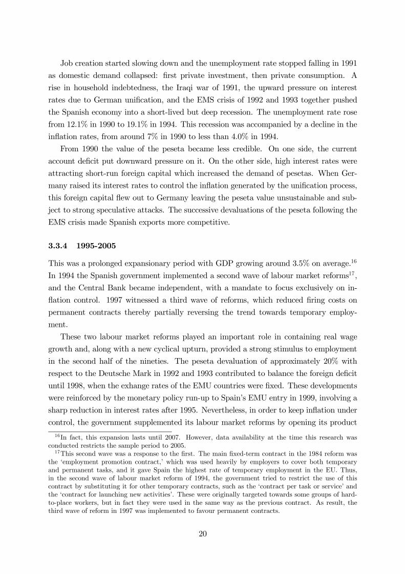
Figure 4 shows that had social security benefits remained constant at its value in
• 1977, the unemployment rate would have been 6.1 percentage points (pp) below theactual 15.4 pp increase over the 1978-1985 recession period,
• 1985, unemployment would have been 0.5 pp above the 6.7 pp decrease over the1986-1991 boom period,28
• 1990, unemployment would have been 2.0 pp below the 8.3 pp increase over the1991-1994 recession period, and
• 1994, unemployment would have been 3.7 pp above the 11.6 pp decrease over the1995-2005 boom period.
According to Figure 5, whereas indirect taxes have negligible contributions during the
first three periods, they put upward pressure on unemployment during the boom period
1995-2005. Had taxes not increased, the unemployment rate would have ended the period
1.6 pp below the actual 11.6 pp decrease. We should point out that the substantial
increase in the indirect tax rate during the long recession of 1978-1985 had virtually no
impact on the unemployment rate.
Figure 6 displays the downward pressure of the stock market activity on the unem-
ployment rate. Had financial wealth29 remained fixed at its value in
• 1977, unemployment would have been 3.5 pp below the 15.4 pp increase over the1978-1985 recession,
• 1985, unemployment would have been 2.3 pp above the 6.7 pp decrease over the1986-1991 boom,
• 1990, unemployment would not have been influenced over the 1991-1994 recession,30
and
• 1994, unemployment would have been 2.5 pp above the 11.6 pp decrease over the1995-2005 boom years.
28Note that during this period benefits hardly change.29Recall that we use the Phelps normalisation to describe the stock market performance, i.e. the (log
of) ratio of(real stock market index to labour market productivity.30This is no surprise as financial wealth is rather stable during these years.
29
Figure 4. Social security benefits: evolution and unemployment effects
a. Evolution
7
8
9
10
11
12
13
14
15
1977 1981 1985 1989 1993 1997 2001 2005
b. 1978-1985 c. 1986-1990
4
6
8
10
12
14
16
18
20
1977 1978 1979 1980 1981 1982 1983 1984 1985
Simulated trajectory
Actual trajectory
4.2%
19.6%
13.5%
12
13
14
15
16
17
18
19
20
1985 1986 1987 1988 1989 1990
Simulated trajectory
Actual trajectory
12.9%
19.6%
13.4%
d. 1991-1994 e. 1995-2005
12
13
14
15
16
17
18
19
20
21
22
1990 1991 1992 1993 1994
Simulated trajectoryAc tual t rajectory
12.9%
21.2%
19.2%
6
8
10
12
14
16
18
20
22
1994 1995 1996 1997 1998 1999 2000 2001 2002 2003 2004 2005
Simulated trajectory
Actual trajectory 9.6%
13.3%
21.2%
Note: Simulated trajectories result from fixing social security benefits at years 1977, 1985, 1990 and 1994.
30

Figure 5. Indirect taxes: evolution and unemployment effects
a. Evolution
6
7
8
9
10
11
12
13
1977 1981 1985 1989 1993 1997 2001 2005
b. 1978-1985 c. 1986-1990
4
6
8
10
12
14
16
18
20
1977 1978 1979 1980 1981 1982 1983 1984 1985
Simulatedtrajectory
Actualtrajectory
4.2%
19.6%
18.8%
12
13
14
15
16
17
18
19
20
1985 1986 1987 1988 1989 1990
Simulated trajectory
Ac tual t rajectory
12.9%
19.6%
12.4%
d. 1991-1994 e. 1995-2005
12
13
14
15
16
17
18
19
20
21
22
1990 1991 1992 1993 1994
Simulated t rajec tory
Ac tual trajectory
12.9%
21.2%
6
8
10
12
14
16
18
20
22
1994 1995 1996 1997 1998 1999 2000 2001 2002 2003 2004 2005
Simulated t rajectory
Ac tual trajectory9.6%
8.0%
21.2%
Note: Simulated trajectories result from fixing indirect taxes at years 1977, 1985, 1990 and 1994.
31

Figure 6. Financial wealth: evolution and unemployment effects
a. Evolution
3.5
4.0
4.5
5.0
5.5
6.0
1977 1981 1985 1989 1993 1997 2001 2005
b. 1978-1985 c. 1986-1990
4
6
8
10
12
14
16
18
20
1977 1978 1979 1980 1981 1982 1983 1984 1985
Simulated trajectoryActual t rajectory
4.2%
19.6%
16.1%
12
13
14
15
16
17
18
19
20
1985 1986 1987 1988 1989 1990
Simulated trajectory
Actual trajectory
12.9%
19.6%
15.2%
d. 1991-1994 e. 1995-2005
12
13
14
15
16
17
18
19
20
21
22
1990 1991 1992 1993 1994
Simulated trajectory
Ac tual trajectory
12.9%
21.2%
21.1%
6
8
10
12
14
16
18
20
22
1994 1995 1996 1997 1998 1999 2000 2001 2002 2003 2004 2005
Simulated trajectory
Ac tual t rajec tory9.6%
12.1%
21.2%
Note: Simulated trajectories result from fixing financial wealth at years 1977, 1985, 1990 and 1994.
32

The contributions of foreign demand are depicted in Figure 7 and are qualitatively
similar to the contributions of financial wealth. Both variables have an inverse relationship
with unemployment and do not contribute to the evolution of the unemployment rate
over the 1991-1994 recession. But in contrast to financial wealth, which has an upward
trend during the whole sample, foreign demand is characterised by a downward trend.31
Furthermore, foreign demand appears to have a stronger impact on the unemployment
rate than financial wealth. Had foreign demand stabilised at its value in
• 1977, unemployment would have been 4.2 pp below the 15.4 pp increase over the1978-1985 recession,
• 1985, unemployment would have been 5.4 pp above the 6.7 pp decrease over the1986-1991 boom period, and
• 1994, unemployment would have been 5.8 pp above the 11.6 pp decrease over the1995-2005 boom.
Finally, it is clear from the plots in Figure 8 that capital stock accumulation has the
most profound influence on the evolution of the unemployment rate.32 In particular,
• Figures 8b, 8c, and 8e show that, for each period, the simulated final value of
unemployment is very close to its initial actual value. This indicates that (i) the
rise in unemployment during the 1978-1985 "long recession" years, (ii) the fall in
unemployment during the 1986-1991"EU cycle" boom period, and (iii) the fall in
unemployment during the 1995-2005 "EMU cycle" boom years were mostly due to
the swings in the growth rate of capital stock.
• Figure 8d shows that had the capital stock growth remained constant at its 1990value, unemployment would have been 6.6 pp below the 8.3 pp increase over the
1991-1994 "EU cycle" recession years.
31In fact, Spain faces a trade deficit since the late 80s which deteriorates over time.32Bande and Karanassou (2008) examine the dynamics of Spanish regional unemployment rates over
the 1980-1995 period and find that capital stock growth was the main driving force of the unemploymentrate during the 1985-1991 boom and 1991-1995 recession years.
33

Figure 7. Foreign demand: evolution and unemployment effects
a. Evolution
-10.0
-8.0
-6.0
-4.0
-2.0
0.0
2.0
4.0
6.0
8.0
1977 1981 1985 1989 1993 1997 2001 2005
b. 1978-1985 c. 1986-1990
0
5
10
15
20
25
1977 1978 1979 1980 1981 1982 1983 1984 1985
Simulated trajectory
Actual t rajectory
4.2%
19.6%
23.8%
6
8
10
12
14
16
18
20
1985 1986 1987 1988 1989 1990
Simulated trajec tory
Ac tual t rajec tory
12.9%
19.6%
7.5%
c. 1991-1994 d. 1995-2006
12
13
14
15
16
17
18
19
20
21
22
1990 1991 1992 1993 1994
Simulated trajectory
Actual trajectory
12.9%
21.2%
21.5%
2
4
6
8
10
12
14
16
18
20
22
1994 1995 1996 1997 1998 1999 2000 2001 2002 2003 2004 2005
Simulated trajectory
Actual trajectory
9.6%
3.8%
21.2%
Note: Simulated trajectories result from fixing foreign demand at years 1977, 1985, 1990 and 1994.
34

Figure 8. Capital stock accumulation: evolution and unemployment effects
a. Evolution
2.0
2.5
3.0
3.5
4.0
4.5
5.0
1977 1981 1985 1989 1993 1997 2001 2005
b. 1978-1985 c. 1986-1990
0
2
4
6
8
10
12
14
16
18
20
1977 1978 1979 1980 1981 1982 1983 1984 1985
Simulated trajectory
Actual t rajectory
4.2%
19.6%
3.8%
12
14
16
18
20
22
24
1985 1986 1987 1988 1989 1990
Simulated trajec tory
Actual trajectory
22.0%
19.6%
12.9%
d. 1991-1994 e. 1995-2005
12
13
14
15
16
17
18
19
20
21
22
1990 1991 1992 1993 1994
Simulated trajectory
Ac tual t rajectory
12.9%
21.2%
14.6%
8
10
12
14
16
18
20
22
1994 1995 1996 1997 1998 1999 2000 2001 2002 2003 2004 2005
Simulated trajectory
Actual trajectory
9.6%
20.1%21.2%
Note: Simulated trajectories result from fixing capital stock accumulation at years 1977, 1985, 1990 and 1994.
35

6 Regime Changes in Capital Accumulation
The simulations in the previous section showed that capital accumulation is the most
crucial factor in driving the unemployment movements over each of the four distinct
periods in our sample. In what follows we elaborate on this finding by evaluating the
impact of the regime changes in the growth rate of capital stock on the unemployment
rate trajectory. We identify the number and longevity of the regimes embedded in the
growth rate of the capital stock by estimating its kernel density function.33
A stationary time series with different regimes is characterised by a multimodal density
of its frequency distribution, the number of modes corresponding to the number of regimes.
In particular, a unimodal kernel density indicates that a unique regime exists with mean
equal to the value of the mode. On the other hand, a variable with two regimes displays
a bimodal kernel density with a "valley point" dividing the observations in the sample.
The data points are grouped in the two regimes depending on whether they lie to the left
or to the right of the "valley point". The kernel density analysis of the two-regime case
can easily be extended to account for three or more regimes.
Naturally, when the variable is characterised by one regime, this is taken to be perma-
nent. For multimodal kernel densities we distinguish between permanent and temporary
regimes and identify them as follows. The variable starts in one regime (say, A) in the
beginning of the sample, and then moves to another regime (say, B) at some later point
in time. If the variable reverses to regime A before the end of the sample, then regime
B is temporary and regime A is permanent. On the other hand, if the variable stays in
regime B by the end of the sample then both regimes are permanent ones.
The bimodal kernel density in Figure 9a indicates that the growth rate of capital stock
is characterised by two regimes. According to Figure 9b these regimes are permanent, the
"high" regime with mean 6.8% lasts until 1976 when capital stock growth enters the "low"
regime with mean 3.7%. This permanent capital accumulation downturn accompanies,
strikingly well, the higher unemployment rates since 1978 (see Figure 1).
Finally, 1978 onwards, we evaluate the unemployment impact of the permanent de-
crease in the growth rate of capital stock as follows. We simulate the steady state of the
labour market model (in Tables 3-5) under two scenarios over the 1978-2005 period: (i)
capital stock growing at 6.8%, and (ii) capital stock growing at 3.7%. The reason for
simulating the steady-state of the model is that we want to measure the effect of the
permanent shift in the growth rate of the capital stock net of the lagged adjustments
present in the labour market. The difference between the two simulated time paths of the
33Raurich, Sala and Sorolla (2006), for the EU and the US, and Karanassou, Sala, and Salvador (2008b),for the Nordic countries, use the kernel density analysis to evaluate the relationship of unemploymentand capital accumulation.
36
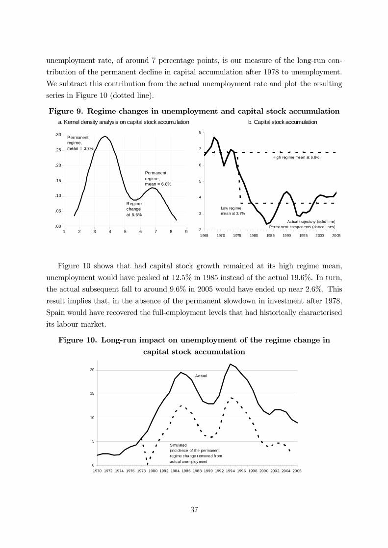
unemployment rate, of around 7 percentage points, is our measure of the long-run con-
tribution of the permanent decline in capital accumulation after 1978 to unemployment.
We subtract this contribution from the actual unemployment rate and plot the resulting
series in Figure 10 (dotted line).
Figure 9. Regime changes in unemployment and capital stock accumulation a. Kernel density analysis on capital stock accumulation b. Capital stock accumulation
.00
.05
.10
.15
.20
.25
.30
1 2 3 4 5 6 7 8 9
Permanentregime,mean = 6.8%
Permanentregime,mean = 3.7%
Regimechangeat 5.6%
2
3
4
5
6
7
8
1965 1970 1975 1980 1985 1990 1995 2000 2005
High regime mean at 6.8%
Ac tual t rajec tory (solid line)Permanent components (dotted lines)
Low regimemean at 3.7%
Figure 10 shows that had capital stock growth remained at its high regime mean,
unemployment would have peaked at 12.5% in 1985 instead of the actual 19.6%. In turn,
the actual subsequent fall to around 9.6% in 2005 would have ended up near 2.6%. This
result implies that, in the absence of the permanent slowdown in investment after 1978,
Spain would have recovered the full-employment levels that had historically characterised
its labour market.
Figure 10. Long-run impact on unemployment of the regime change incapital stock accumulation
0
5
10
15
20
1970 1972 1974 1976 1978 1980 1982 1984 1986 1988 1990 1992 1994 1996 1998 2000 2002 2004 2006
Simulated(incidence of the permanentregime change removed fromactual unemployment
Ac tual
37

7 Conclusions
In this paper we analysed the chain reaction theory (CRT) of unemployment through
a stylised labour market model, and showed that the interplay of the dynamics and
spillovers in the multi-equation system give rise to the phenomenon of frictional growth.
The implications of frictional growth are:
1. unemployment does not gravitate towards its natural rate, since the long-run un-
employment rate equals its NRU plus frictional growth;
2. the unemployment rate cannot be decomposed into cyclical (short-run) and "trend"
(long-run) components;
3. trended exogenous variables can be included in CRT models and, thus, are allowed
to influence the unemployment rate trajectory.
We applied the CRT to the Spanish economy over the 1970-2005 period by estimating
a dynamic system of labour demand, real wage, and labour supply equations with spillover
effects. We found that, although variables which are among the conventional wisdom’s
favourite causes of unemployment (i.e. social security contributions, indirect taxes, and
financial wealth) do matter, capital accumulation is the most important driving force of
unemployment. Furthermore, foreign demand had a substantial impact on the ups and
downs of unemployment, especially during the "EU cycle" of 1986-1990 and the "EMU
cycle" of 1995-2005.
The finding of capital stock growth as the main determinant of the unemployment rate
is in tandem with reality (see Figure 11), and supports the literature on the role of capital
accumulation in the evolution of unemployment (Rowthorn, 1995, 1999; Gordon, 1997;
Arestis and Biefang-Frisancho Mariscal, 2000; Karanassou and Snower, 2004; Blanchard,
2005; Arestis, Baddeley and Sawyer, 2007; and Karanassou, Sala and Salvador, 2008b).
Figure 11. Actual capital-unemployment relationship
0
4
8
12
16
20
24
2
3
4
5
6
7
8
1970 1975 1980 1985 1990 1995 2000 2005
unem
ploy
men
t rat
e %
capital stock growth %
capital accumulation
unemployment rate
38

Our findings indicate that the preoccupation of macroeconomists with the estimation
of the NRU, quite often serves as an end to itself and does not provide the means to
understand what really matters for the evolution of unemployment. We argue that the
unemployment problem can be better addressed by estimating CRT models, and mea-
suring the unemployment contributions of the "usual suspects" (e.g. wage-push factors)
along with those of growing exogenous variables (such as capital stock).
References[1] Arestis, P. and Biefang-Frisancho Mariscal, I. (2000): “Capital stock, unemployment and
wages in the UK and Germany”, Scottish Journal of Political Economy, vol. 47 (5), pp.487—503.
[2] Arestis, P., Baddeley, M. and Sawyer, M. (2007): “The relationship between capital stock,unemployment and wages in nine EMU countries”, Bulletin of Economic Research, vol. 59(2), pp. 125-148.
[3] Bande, R. and Karanassou, M. (2008): “Labour market flexibility and regional unem-ployment rate dynamics: Spain 1980-1995,” Papers in Regional Science, forthcoming,doi:10.1111/j.1435-5957.2008.00165.x.
[4] Bentolila, S. and O.J. Blanchard (1990): “Spanish unemployment”, Economic Policy, vol.10, pp. 233-281.
[5] Blanchard, O. (2005): “Monetary policy and unemployment”, in Semmler. W. (ed.), Mon-etary Policy and Unemployment - US, Euro-Area, and Japan, Routledge, London.
[6] Blanchard, O.J. and J. Wolfers (2000): “The Role of Shocks and Institutions in the Rise ofEuropean Unemployment: The Aggregate Evidence”, The Economic Journal, 110, March.
[7] Cross R., J. Darby, J. Ireland, and L. Piscitelli (1999): “Hysteresis and unemployment: apreliminary investigation”, Computing in Economics and Finance, 5th International Con-ference, Boston.
[8] Dolado, J.J., C. García-Serrano and J.F. Jimeno (2002): “Drawing lessons from the boomof temporary jobs in Spain”, The Economic Journal, vol. 112 (480), pp. F270-F295.
[9] Dolado, J.J. and J.F. Jimeno (1997): “The Causes of Spanish Unemployment: A StructuralVAR Approach”, European Economic Review, vol. 41, pp. 1281-1307.
[10] Dolado, J., Malo de Molina, J.L. and Zabalza, A. (1986): “Spanish industrial unemploy-ment: Some explanatory factors”, Economica, vol. 53, pp. 313—334.
[11] Eichengreen, B. (2000): “The EMS Crisis in Retrospect”, NBER Working Paper No. 8035.
[12] García de Blas, A. (1985): “Unemployment benefits in Spain and other European OECDcountries”, International Labour Review, vol. 124 (2), pp. 147-160.
[13] Güell, M. and B. Petrongolo (2007): “How binding are legal limits? Transitions fromtemporary to permanent work in Spain”, Labour Economics, vol. 14 (2), pp. 153-183.
39

[14] Garrido, L. and L. Toharia (2004): “What does it take to be (counted as) unemployed?The case of Spain”, Labour Economics, vol. 11, pp. 507-523.
[15] Karanassou, M., H. Sala and P.F. Salvador (2008a): “The (IR)relevance of the NRU forpolicy making: The case of Denmark,” Scottish Journal of Political Economy, vol. 55 (3),pp. 369-392.
[16] Karanassou, M., H. Sala and P.F. Salvador (2008b): “Capital Accumulation and Unem-ployment: New Insights on the Nordic Experience”, Cambridge Journal of Economics,forthcoming, doi:10.1093/cje/ben022.
[17] Karanassou, M., H. Sala and D.J. Snower (2003): “Unemployment in the European Union:A Dynamic Reappraisal”, Economic Modelling, vol. 20 (2), pp. 237-273.
[18] Karanassou M., Sala H., and D. J. Snower (2008): “Phillips Curves and UnemploymentDynamics: A Critique and a Holistic Perspective”, Journal of Economic Surveys, forth-coming.
[19] Karanassou, M. and D.J. Snower (2004): “Unemployment Invariance”, The German Eco-nomic Review, vol. 5 (3), pp. 297-317.
[20] Layard, R., Nickell, S.J. and Jackman, R. (1991): Unemployment: Macroeconomic Perfor-mance and the Labour Market, Oxford: Oxford University Press.
[21] Phelps, E. S. (1994): Structural Booms: The Modern Equilibrium Theory of Unemployment,Interest and Assets, Harvard University Press, Cambridge (MA).
[22] Phelps, E. and G. Zoega (2001): “Structural booms: productivity expectations and assetvaluations”, Economic Policy, vol. 32, April, pp. 85-126.
[23] Pesaran, M.H. and Y. Shin (1999): “An Autoregressive Distributed-Lag Modelling Ap-proach to Cointegration Analysis” in Econometrics and Economic Theory in the TwentiethCentury: The Ragnar Frisch Centennial Symposium, edited by Strom, S., Cambridge Uni-versity Press, pp. 371-413.
[24] Pesaran, M.H., Shin, Y. and Smith, R.J. (2001): “Bounds testing approaches to the analysisof level relationships”, Journal of Applied Econometrics, vol. 16, pp. 289-326.
[25] Polo, C. and F. Sancho (1993): “An analysis of Spain’s integration in the EEC”, Journalof Policy Modeling, vol. 15 (2), pp. 157-178.
[26] Raurich, X., H. Sala and V. Sorolla (2006): “Unemployment, Growth and Fiscal Policy:New Insights on the Hysteresis Hypotheses”, Macroeconomic Dynamics, vol. 10 (3), pp.285-316.
[27] Rowthorn, R. (1995): “Capital formation and unemployment”, Oxford Review of EconomicPolicy, vol. 11 (1), pp. 26-39.
[28] Rowthorn, R. (1999): “Unemployment, wage bargaining and capital-labour substitution”,Cambridge Journal of Economics, vol. 23, pp. 413-425.
[29] Sosvilla-Rivero, S. and J.A. Herce (2008): “European cohesion policy and the Spanisheconomy: A policy discussion case”, Journal of Policy Modeling, vol. 30, pp. 559-570.
40