Embed Size (px)
Citation preview

The Review of Economic Studies Ltd.
Econometric Business Cycle ResearchAuthor(s): J. TinbergenSource: The Review of Economic Studies, Vol. 7, No. 2 (Feb., 1940), pp. 73-90Published by: The Review of Economic Studies Ltd.Stable URL: http://www.jstor.org/stable/2967472Accessed: 29/03/2010 18:44
Your use of the JSTOR archive indicates your acceptance of JSTOR's Terms and Conditions of Use, available athttp://www.jstor.org/page/info/about/policies/terms.jsp. JSTOR's Terms and Conditions of Use provides, in part, that unlessyou have obtained prior permission, you may not download an entire issue of a journal or multiple copies of articles, and youmay use content in the JSTOR archive only for your personal, non-commercial use.
Please contact the publisher regarding any further use of this work. Publisher contact information may be obtained athttp://www.jstor.org/action/showPublisher?publisherCode=resl.
Each copy of any part of a JSTOR transmission must contain the same copyright notice that appears on the screen or printedpage of such transmission.
JSTOR is a not-for-profit service that helps scholars, researchers, and students discover, use, and build upon a wide range ofcontent in a trusted digital archive. We use information technology and tools to increase productivity and facilitate new formsof scholarship. For more information about JSTOR, please contact [email protected].
The Review of Economic Studies Ltd. is collaborating with JSTOR to digitize, preserve and extend access toThe Review of Economic Studies.
http://www.jstor.org

Econometric Business Cycle Research
I. INTRODUCTORY
In recent years various attempts have been made to construct econometric models of the business cycle mechanism.' Some of them are very simple, others more complicated; some pay more attention to the mathematico- economic set-up, others give special care to a statistical determination of the coefficients involved. The latter group is notable for, in particular, the model by Radice of the post-war United Kingdom,2 that by De Wolff of post-war Sweden,3 and my own attempts for the Netherlands and the United States.4 As far as I am myself concerned, a " model under construction " is that for the United Kingdom between I870 and I9I4.5
An essential feature of an econometric model is, I think, that it combines mathematico-economic treatment with statistical measurement of some type. The ultimate objectives of these models are the same as of any system of business cycle research, viz. (i) to explain historical events; (ii) to forecast future developments under certain conditions; and (iii) to indicate the prob- able consequences of measures of business cycle policy. Within the framework of these ultimate objectives, one may distinguish more proximate objectives. These may be separately stated for the economic and the statistical parts of the task. The objectives of the economic part are, to my mind:
(a) to clarify notions and assumptions of various theories and to localise differences of opinion;
(b) to find the complete implications of any set of assumptions as to type.of movement resulting, influence of given types of policy, etc.
The objectives of the statistical part are: (a) either, more modestly, to find such values for coefficients, etc., as are
not contrary to observation (b) or, more ambitiously, to prove, under certain conditions, something
to be true or not true.
1 Apart from the examples to be quoted in notes 2 to 5 we may mention the following: R. Frisch: " Propagation Problems and Impulse Problems in Dynamic Economics,"
Economic Essays in Honour of Gustav Cassel, London, I933. M. K4ecki: " A Macrodynamic Theory of the Business Cycle," Econometrica, 3 (I935),
p. 327. E. Lundberg: Studies in the Theory of Economic Expansion, London, I937.
B. A. Chait: Les fluctuations dconomiques et l'interd6pendance des marchds, Brussels, I938.
2 E. A. Radice: "A Dynamic-Scheme for the British Trade Cycle, 1929-I937," Econometrica 7 (I939), p. I.
3 To be published in the near future. 4 J. Tinbergen: An Econometric Approach to Business Cycle Problems, Paris, I937, and
Business Cycles in the United States of America, I9I9-I932 (Statistical Testing of Business Cycle Theories, II), League of Nations, Geneva, 1939.
G. Lutfalla is working on a similar model for France.
73

74 THE REVIEW OF ECONOMIC STUDIES
It goes without saying that the use of mathematics is only a question of language; it does not imply any a priori choice of economic theory.
The statistical instruments used may be different. A frequent mis- understanding is that only multiple correlation analysis is used, or even ad- mitted. Any method yielding results may be used, of course.
Recently there has been some discussion on the nature and the limitations of the econometric method.' I gladly accept, therefore, the invitation of the editors of this REVIEW, to go into some more detail concerning the method. Since the subject is almost ripe for a text-book-at any rate as far as its extent is concerned-I must necessarily restrict myself. I shall try to do this in an efficient way, and to fill some gaps by references to other papers.
2. MATHEMATICAL BUSINESS CYCLE THEORY:
THE FOUNDATIONS
2.I. THE "ARROW SCHEME " AND ELEMENTARY EQuATIoNs
Turning, first, to the mathematico-economic part of the work, I think this may be characterised as the construction of a scheme for the utilisation of business cycle theories. It consists in indicating the logical structure of the
business cycle mechanism. CHART I A graphic representation,
given in Chart i, may A serve as a starting point.
This scheme shows, in each (vertical) column the
B ~~~~~~~~~~list of phenomena (vari- ables) included: A, B, C . . . In each (horizontal)
C / 82.S/ t row the course of time is
C 6 - represented; i.e. the con- secutive dots represent one phenomenon at consecutive
D * * s w v unit time intervals. De- noting these by a suffix,
t-l t t+l t+2 tt3 tAhe dots represent, e.g. Al) A2,A3, A 4, etc. The
extent of each of them, if A is a measurable phenomenon, could be plotted in a third dimension, e.g. per- pendicular to the plane. We shall not, however, go into that now. Any definite theory tells us how a given change at moment t in A acts on other phenomena at other moments. Suppose the theory is that it acts on B without lag and on C with a lag of one time unit, i.e. A (t) acts on C(t+ I). This is indicated by
I Cf. especially Mr. Keynes's review of Vol. I of my League of Nations study: " Statistical Testing of Business Cycle Theories, I: A Method and its Application on Investment Activity," in the Economic Journal of September, 1939, p. 558.

ECONOMETRIC BUSINESS CYCLE RESEARCH 75
the arrows from A (t) to B(t) and from A (t) to C(t+ I). If, e.g. changes in C are assumed to work on D and A, both with a lag of two time units, this will again be indicated by arrows. A change in A (t) may be said to be a " first" or " direct " " cause " to a change in C(t+i), and a " second" or " indirect cause to a change in D(t+3). All the arrows repeat themselves as long as the model's structure is supposed to remain the same. The more details are con- sidered, the greater the number of arrows. The totality of arrows may be " listed " in two ways, viz. (i) according to the variable from which they start, or (ii) according to the variable at which they end. In the first listing all " effects" of changes in one variable on others are grouped together; in the second all ",causes" of changes in one variable are put into one group. Both lists describe, however, the same mechanism. The latter corresponds to what will, in this paper, be called the system of elementary equations. Each equation indicates how changes in one variable depend on the " causing" changes in other variables.
Let income be Y, price level p, and consumption outlay U'; and let a certain theory assume that consumption outlay depends only on income and price level one time unit before. The arrows ending in U,' will then be only two, one coming from Y,-,, and one from Pt-i The corresponding equation will be 1
Ut'= f(Yt1, t-,) .... .................................. (I)
The function may be given a definite mathematical shape, it may, e.g., be linear:
Ut=vlYt-l + v2Ptl ........ .................. (2)
In that particular case, and in some other cases, it is possible to indicate the influence " of a change A Ytl on U ' ; it will be vA YA1 ; similarly the influence " of a change Apt-, will be v2APti.
A complete theory will contain as many such equations as unknown variables. The economic character of these equations may be one of the following:
(i) a definition, e.g. value equals price times quantity;
(ii) a balance equation, e.g. production = consumption + increase in stocks;
(iii) a technical, natural or institutional connection;
(iv) a reaction equation. The above example on consumption outlay belongs to this class. In general, the more " interesting " equations belong to this class, such as supply and demand equations. They always represent the reaction of groups of individuals or firms on certain economic conditions (incomes, prices, costs, etc.).
1 By unbarred symbols I indicate deviations from the average over the period studied. For the present equation this is indifferent, but for some of the further equations it is essential.

76 THE REVIEW OF ECONOMIC STUDIES
2.2. VARIABLES, COEFFICIENTS, UNSYSTEMATIC TERMS
The example given was a very simple one. In its most complete form elementary equations may contain the following elements:
i. the variable " explained" by that equation (in the example U'); 2. " explanatory" variables (in the example: Y and p); 3. constant coefficients and lags, representing the " structure" of the
model (vl and V2);
4. additional unsystematic terms. These are to be understood in the following way. All the possible causes of changes in the variable to be explained may be subdivided into systematic and non-systematic ones. The subdivision is to some extent arbitrary in that it may depend on the objectives of the study as well as on the behaviour of these causes. Purely accidental causes " obeying the probability laws " will always be classified as non-systematic. The influence of certain types of policy (e.g. tax changes) may, however, be classified in either group, depending on the problems to be solved. Indicating by Ru' the total influence of non-systematic forces, equation (2) may be given the more complete form.
Ut v1Yt i+v2P, 1+Ru1 ...... ........... (3)
Since these unsystematic terms as a rule change suddenly, they are sometimes called " shocks."
5. It may happen that a fifth category of terms appears in an elementary equation, viz. a given function of time F(t). Various possibilities may be distinguished: (i) F(t) may be a trend of any form being a catch-all of all causes
moving only slowly and therefore not interesting for the analysis of rapid fluctuations;
(ii) or it may take the form of a rapidly changing function of time standing for some given " external variable" ; as a special case, this function may be or be assumed to be periodic. External variables are variables relating to non-economic phenomena or to economic variables outside the area considered. If a national economy as a whole is studied, foreign phenomena are external: if one market is studied, phenomena concerning other markets.
2.3. THE DETERMINATION OF THE SYSTEM S MOVEMENTS: THE ELIMINATION PROCESS
If all elementary equations describing the logical structure of a model are known, it is, in principle, possible to find the movements of the system as long as we are given:
(a) the " structure" of the model, represented by the coefficients, the lags, and the trends in the equations;

ECONOMETRIC BUSINESS CYCLE RESEARCH 77
(b) the values of the '' external variables " for all time units;
(c) the " disturbances" represented by the residuals for all time units; and
(d) the " initial values" of one or more of the variables of the problem. Exactly what initial values must be given can only be indicated in each particular case.
The technique by which these movements may be ascertained may be different. The simplest technique is that of " numerical extra-polation." An example is given in section 3.2. Here the propagation of t-he movements is followed step by step; in turn each elementary equation is used to compute one new value for one of the variables.' A more advanced technique consists in the " elimination process." Any two equations containing one variable in common may be combined into a new equation without that variable. In particular this elimination has a meaning if, in any equation, one of the explanatory variables is replaced by the equation explaining that variable. This means that instead of considering a " first cause" we are considering
second causes."
If the price level Pt-i in equation (3) is itself determined by the equation
Pt = Wrt1+W21t1+Rt .................................... (4) involving that
Pt-1 = 7Trt2+7T21t_2+ RPi ................................ (4)
where r is the level of raw material prices, and I that of wage rates,
and, hence, 71lrt-2+?2lt-2 represent cost of production, we may insert this equation into (3), yielding
= vYt ?P2(r2?2lt2).................. (5) As far as a change in Ut' is to be attributed to changes in the price level, this change in Ut' has now been brought back to "deeper causes," viz. " second causes.''
The elementary equations may be said to represent " elementary economic laws," the elimination results in representing " deduced economic laws." The laws of demand and supply, or-Mr. Keynes's "psychological law of consump- tion " are examples of " elementary laws." The law of demand relates quantity demanded to price and other variables (such as e.g. income), that may be called " demand factors." Combining the law of demand and that of supply we get an equation by which either the price or the quantity handled is expressed as a function of " demand factors " and " supply factors." This may be called a deduced law. Similarly a deduced law might be obtained by substituting in the consumption equation (2) the equation telling how incomes depend on other economic phenomena.
1 Good examples are to be found in Lundberg, loc. cit.

78 THE REVIEW OF ECONOMIC STUDIES
In this train of thought there is a whole hierarchy of deduced economic laws of different order. Most of these laws would not be known under separate names. This is one of the reasons why it is so difficult to give a verbal account of the process of elimination and why this process has been called " night train analysis." The final stage is reached if we are left with one single equation containing only one variable. This equation will be called the final equation. It is not always possible to obtain, without using approximates, only one final equation. At a certain stage, a system of equations may be obtained that cannot further be reduced and may be called an irreducible system.
The final equation contains, apart from the values at various time points of the one variable left, a number of terms with unsystematic influences. In equation (5) we already find two such terms; in the final equation there will, in general, be a greater number. Each step in the elimination process brings new ones. Each separate unsystematic influence R is multiplied by one or more coefficients; only the R-term originating from the elementary equation taken at the start has a coefficient equal to i. Thus we see clearly how " shocks " applied to various elementary relations are cumulative and that their influence may be found back in the movements of any variable in the system, damped or magnified in dependence of the coefficients appearing before them. This is the bridge to calculations of " multipliers " in the Kahn sense.'
The performance of the elimination process exhibits very clearly one fundamental difficulty in business cycle theory. In order to be realistic it has to assume a great number of elementary equations and variables; in order to be workable it should assume a small number of them. It is the task of business cycle theory to pass between this Scilla and Charybdis. If possible at all the solution must be found in such simplifications of the detailed picture as do not invalidate its essential features. This should not be forgotten by those urging the introduction of many details into the elementary equations. Of course it may first be attempted to establish a system of very detailed elementary equations and then to simplify them in various alternative ways, in order to find out the differences in results. Such complicated systems as I tried to establish for the United States particularly lend themselves to this sort of experiment.
2.4. THE FLEXIBILITY OF THE METHOD I want to emphasise the great flexibility of the method under discussion.
Often this is not sufficiently recognised by non-mathematical critics. I believe the following features in particular make it possible to fit the scheme to almost any theory:
(i) the number of variables and of equations is free (ii) the number of terms in each equation is free;
(iii) the shape of the functions is free; (iv) the introduction of non-systematic terms is free. This circumstance
opens up the possibility of introducing the influence of " impondera- bilia." 2
I Cf. Business Cycles in the U.S.A., pp. I62-5. 21 have gone into more detail concerning this question in my reply to Mr. Keynes in the
Economic journal.

ECONOMETRIC BUSINESS CYCLE RESEARCH 79
In particular, point (iii) deserves some further attention. It is often thought that the method, particularly if completed by statistical determination of the coefficients and lags, but also in view of the performance of the elimination process, is bound to the assumptions of constant coefficients and lags. The first of these two assumptions is equivalent to linear functions. I should like to recall briefly some remarks I have made, on various occasions, on this point.
i. It is not necessary to restrict ourselves to these hypotheses. There are various ways of avoiding them. We may introduce quadratic functions, or more complicated functions. Instead of (2) we may have an equation:
v,Yt ?v2Pt +v22P2l. Or we may sub-divide the relevant interval of any variable into intervals in each of which separately the relations are linear.' A supply function showing the feature of saturation may be approxi- mated by two straight lines. Lags may be assumed to be different in various conditions.
2. Using linear functions does not mean such a serious restriction as is often thought.
Linearity is not synonymous with proportionality.2 Over small intervals almost any function may be approximated by a linear one. This is also true in the case where a coefficient is believed to depend on other variables. Suppose the influence of income on consumption outlay is assumed to be dependent on prices. This would mean that in our equation (2) v1 would be a function of Pt-i, say; therefore v- = v(Pt-,)*
In order to make clear exactly what this means, it will be better to start with equation (2) in another form, viz. using absolute values of variables Ut', Yt, etc. instead of deviations from the average. It then runs:
Ut = V1(Pt 1)Yt_,+v2Pt,?+C ................................ () where C is a constant. As a first approximation for small intervals vj(pt_,) may be assumed to be a linear function:
V1 = Pt-1 Hence we get:
Ut = VioYt-?+V1iPt1- Yt-1+v2Pt 1+C This may again be brought into the form
U +Ut = vlOY+vlOYt.l+vll(P+Pt-1)(Y+Ytel)+v2(P+Ptgl)+C or:
U'+ Ut' (v,OY+v,,PY+v2P+C) +Vloyt-l+vllPyt + V11YPt-? +11Pt-Yt-+ V2Pt-1
This may be contracted to: UK+ ut: = C'+v'oYt-?v't2Pt-1+v11Pt1Y
1 As an example, cf. the treatment of stock exchange speculation in Business Cycles in the U.S.A.
2 Cf. A Method and its Application to Investment Activity, p. i6.

8o THE REVIEW OF ECONOMIC STUDIES
where C', v'10 and V'2 are new constants; if we use deviations from the average again, the terms vjjp_1Ytl will consist, as a rule, of small terms of the second order, being a product of deviations which are, as a rule, not large in comparison to the average values. The last term may then be left aside; and the constant term C' will cancel out against U':
Ut = 1'ioYt 1+v'2Pt-1 The influence of p on the coefficient of Y,_1 is not, by these approximations, neglected, but hidden in the new coefficient v'2 which is different from v2.
3. Even if we assume curvilinearity in our relations and " coefficients depending on other variables," etc., we come back, in the end, to coefficients that are constant (v22 and vll in the above examples). But that is essential for any theory that really deserves the name. Theory always means reducing variable things to constancy. In the simplest example of theoretical economics, viz. the use of the concept of demand curve, it takes the form of reducing fluctuations in quantity to given fluctuations in prices by some constant scheme. Complicated theories will establish the constancy in a complicated way, but will, in the end, also look for something constant. Describing pheno- mena without any sort of regularity or constancy behind them is no longer theory. An author who does not bind himself to some " laws " is able to it prove " anything at any moment he likes. But then he is telling stories, not making theory.
3. MATHEMATICAL BUSINESS CYCLE THEORY: SOME RESULTS
3. I. RESULTS FOR THE SETTING OF THE PROBLEM
What, now, is the sort of knowledge we can obtain by mathematical business cycle theory ?
First, we can already achieve considerable improvement in the setting of the Problems.
(i) We are able to find whether a given theory is complete in the sense of using a number of equations equal to the number of unknowns. In itself it is not very important to reach this stage, and the Lausanne school has sometimes-and rightly, I think-been ridiculed for stopping after having found that there are as many equations as unknowns. Nevertheless, there is one thing that is worse, viz. finding that there are not the -same number! In how many well-known essays on the cycle has it been stated carefully what their number is ?
(ii) We are forced to state clearly what relations we assume to exist. For example, I find it difficult to understand whether some theories that assume an influence of the interest rate on commodity stocks have in mind:
(a) an influence of interest rates on stocks, or (b) an influence of interest rates on the increase in stocks during
the unit time period considered.

ECONOMETRIC BUSINESS CYCLE RESEARCH 8I
Another example: many authors do not state whether or not they assume lags to exist in the relations they use. Mathematical treatment would force them to choose.
(iii) Mathematical treatment in the way indicated above provides a good means of " locating " differences of opinion between different theories. One can tell in what relation or, as the case may be, in what term the theories diverge. Logical classification of theories becomes possible.' One example of classification of outstanding importance is the distinction to be made between theories that consider the systematic terms as more essential, and theories that consider the non-sysfematic ones as more essential-explicitly or implicitly. As a rule, current information on the economic situation gives much more attention to " new events," corresponding to our non-systematic terms; it seems to be based upon the implicit assumption that these new events are very important.
(iv) Apart from the general remarks just made, one or two special examples of the advantages of our method may be given.
What does the term " a flexible economy" mean ? I think two elements are hidden in this concept, which are often not disentangled sufficiently, although they differ pretty much in their relation to the expected advantages (or disadvantages) attached to them. The reaction on one variable or another may be
(a) strong or weak, and, independently of this, (b) rapid or slow.
Strength as well as rapidity seem to be elements of " flexibility"; their influence on the damping of business cycles may differ, however, considerably.
For instance, what should we do about the famous catch-all that two phenomena are " mutually related" ?--a statement sometimes arrived at as the philosophical endpoint of a discussion-dark as so much philosophy. I believe it can be given a clear interpretation with our " arrow diagram." It may then be stated far better in the following way-taking one relation as a possible example: A(t) influences B(t+i), and at the same time B(t) influences A (t+ 2).
3.2. THE TYPES OF MOVEMENTS; THEORIES OF THE CYCLE v. THEORIES OF THE CUMULATIVE PROCESS
The second type of insight we can get, I think, from mathematical treatment, is a systematic insight into the types of movements that economic systems may perform. There is a piece of science of considerable extent-and use, I think-to be built on the basis of our system of equations even before any special economic meaning is given to the variables involved. I shall try to give some examples.
1 I tried to work out this idea in Business Cycles in the U.S.A., pp. I8I-3.
6 Vol. 7

82 THE REVIEW OF ECONOMIC STUDIES
(i) The nature of the central problem in dynamic economics is different from that in static economics. In the latter it is: what is the (constant) value of any variable if the system is in equilibrium ? In the former it is: what is the course in time of each variable ?
(ii) What movements does a given economic system (i.e. an economy of which the elementary equations are given) show ? (A) It is useful to distinguish between undisturbed and disturbed
movements. Undisturbed movements occur during any period where no new unsystematic external causes occur. New unsys- tematic external causes are synonymous with disturbances. We start by considering undisturbed movements.
(B) Further, we provisionally restrict ourselves to systems of linear equations. It may then be shown in a general way that the movements that any variable in the system shows are super- positions of one or more of the following types of components: (a) a constant level (this in a sense is not a movement, but, if
one likes, a basis level from which the other movements may be measured);
(b) an external trend movement, given by the evolutionary external factors (e.g. growth of population-if we assume it to be independent of the economic situation-or of tech- nical knowledge; but not, strictly speaking, growth of capital );
(c) an external periodic movement (e.g. seasonal fluctuations) or other non-trend movement (e.g. due to systematic external causes such as international prices);
(d) damped exponential movements, i.e. deviations forming a geometric series of falling absolute values;
(e) anti-damped exponential movements, i.e. deviations the values of which form an increasing geometric series;
(f) damped periodic movements, i.e. movements whose time shape is a damped sine curve;
(g) anti-damped periodic movements.' The constant level (a) would alone be present if the system of equations
were static in the strict sense, i.e. that only (i) variables that relate to one and the same time unit and (2) constant coefficients and additional terms are present.
The external trend movement (b) will appear as soon as e.g. a term growing linearly with time, representing e.g. the movement of population or of knowledge, comes into one or more of the equations. Similarly, the external non-trend movements will come in with the introduction of given functions of time.
1 Strictly speaking, a linear movement in time, due to internal causes, should be added for the case where two roots of the characteristic equation coincide, etc. This will be disregarded.

ECONOMETRIC BUSINESS CYCLE RESEARCH 83
The internal or endogenous movements (d) to (g) are only possible if not all the variables relate to the same time unit (or if differential coefficients or integrals occur, which, in a sense, means the same). Even then they may, for some special values of the initial values of the variables, be absent. In simple cases, these special values are comparable to equilibrium values in the static sense, i.e. values that would remain if no data were to change. In more com- plicated cases, things are less easy.' One can only get an idea of this type of problem by " playing" with some of the models. I have given a very simple example in Business Cycles in the United States (pp. I5-I8). This example may be given a somewhat different form in order to demonstrate one or two principles of outstanding importance.
Let the total of all expenditure on final consumption and net investment in unit time period t be Xt, and income Zt. Then, as a first elementary equation we have:
zt xt indicating that income will simply be equal to these expenditures. The second equation has to answer the question, How are these expenditures themselves determined ? Here, in order to state our present problem in the simplest way possible and to couple it as little as possible to specific economic theories, we start from some very general principles. Expenditure will be based-directly or indirectly-on income some time ago; there will be a lag. This lag may be a distributed one, so that in the simplest case there are two lags included, say, of one and of two time units. The coefficients corresponding to these two lags may be of opposite sign. In this general principle the special case is included where expenditure is based on expected income, so far as these expectations are themselves based on
(a) income at prior moments, and even on (b) the rate of increase in income formerly observed.
Non-systematic causes are disregarded for the moment. As our second equation we therefore get:
Xt- 1Z-l+62Zt-2+C (ell e2' C, constants)
Using the first equation, we have at once the final equation: Zt = e1Zt-1+e27t-2+C
The elimination process is very simple now, since we purposely combined direct and indirect influences without further discussion and so came back at once to Zt-, and Zt-2. For the moment our problems lie elsewhere.
In order to fix the ideas, we choose some particular values, viz. el = +I.6, 2= -I, C = 4.
We now have a case without external movements, since trends or non- trend external movements are assumed not to occur. Components (b) and (c)
1 I treated some questions relating to this matter in An Econometric Approach and particularly in Fondements mathematiques de la stabilisation des affaires, Paris, 1938, and in " Sur la d6termina- tion statistique de la position d'6quilibre cyclique," Revue de l'Institut International de Statistique, I936, p. I73 (with English summary).
6*

84 THE REVIEW OF ECONOMIC STUDIES
are absent, therefore. It would not however, complicate matters to introduce (b) into C, by assuming C to depend linearly in time.
Component (a) is present. It can be shown to be Z = I0. It may be tested by the non-mathematical reader by giving all Z's this value; then the equation is satisfied:
I0 = I.6 x IO-I X IO+4
The other components are found in the simplest manner by measuring Z in a new way, viz. as deviations from io. Writing Z' for Z- io, we get the fol- lowing equation for Z':
zt i.6Z't t-Z't-2 i.e. an equation without constant terms. This equation enables us to determine the development of Z', if two values are given. It is worth while to give an example. Let Z'0 o, Z'1 = i. We easily find the figures of the following table (to be called " example I "):
z 2 z'3 Z'4 Z'5 z'6 Z'7 z'8 z'9 z'10 z'11
+I.6 +I.56 +0.9 -O.I -i.i -i.6 -I.5 -o.8 +0.2 +I.I
It can be shown that this periodic movement will occur irrespective of the initial values chosen.
Suppose now that the structure of the model were different and that the coefficient i.6 were 2.2. If again Z'0 0 and Z'1 - I, we should now find the following development (to be called "example II "):
z'2 Z3 Z4 Z5 Z6 Z7
+2.2 +3.84 +6.2 +9.8 +I5.3 +23.8 The movement is now one-sided (anti-damped exponential) and can
equally be shown to be so, independently of the initial values. (The movement may, however, be directed towards - oc instead of towards + oo.)
I want to draw two conclusions from the comparison of these two examples. In economic terms, example I contains a theory -of the cycle, i.e. of the cumu-
lative Process as well as of the turning Point ; whereas example II only contains a theory of the cumulative process. If example II had been the outcome of some set of economic hypotheses, a separate theory of the turning point would have been necessary. Generally speaking, it is sometimes necessary to give a separate theory of the turning point; sometimes, however, it is superfluous. There are scrupulous authors who give a theory of the turning point where it would perhaps not be necessary; there are other authors who think that they are giving a theory of the cycle, where they only give one of a cumulative process. How can we know whether a theory is of type I or type II ? Often not by verbal treatment; our example II need not differ verbally from example I; the same phenomena may be included in both; only the intensity with which some of them act need be different.
Considering example I we may, then, ask with Mr. Keynes 1: how does reversal come in ? We see, before our eyes, that Z'3<Z'2. What is the reason ? It is not that some new phenomenon enters. Qualitatively the same forces
1 Loc. cit.

ECONOMETRIC BUSINESS CYCLE RESEARCH 85
are at work as before. It is " simply" the change in relative strength of the positive and the negative forces that alters the balance.
In order to see this in more detail, let us repeat the first two figures in example I and their genesis. For t =2z and t 3 we have:
Z 2 i.6Z'-Z'0 i.6 x i -o I.6 Z=3 i.6Z'2-Z' 1 i.6X i.6-i I.56
In Z'2, the positive influence of Z'1 is large, the negative influence of Z'0 zero, since Z'0 is zero. In Z'3, the positive influence of Z'2 is even larger, but the negative force, -Z'1, has grown a little bit more.
That change in relative strength is itself a consequence of the laws governing-in our example-expenditure. It seems to be difficult, if not idle, to attribute it to some special cause. One may construct other examples where reversal does come in owing to some specific reason, some " ceiling " in credits or employment or still other things. But it does not follow that turning points can only be explained that way. I think this is a rather widespread misunder- standing among non-mathematical theorists.
Example II must not be misunderstood. Its ever-increasing figures may, perhaps, soon reach some impossible level. Does this prove that the theory behind it is erroneous and that, therefore, the example has no significance at all ? I should prefer to put it in anoth-er way. The theory is only valid within a certain interval of values for Z'. If that theory itself leads to values outside that range we must stop applying it. And the conclusion remains: that theory cannot explain a turning point.
3.3. STABILITY OF EQUILIBRIUM
Much more could be said about movements of systems. I have done so on other occasions; and hope to unite all this within a larger framework. But it would take us too far now. We may proceed with another subdivision of the subject that equally illustrates what mathematical treatment teaches us.
(iii) What is to be understood by " business cycle stabilisation " ? We shall try to give this notion a clear-cut meaning in the following way-which, of course, need not be the only possible way. Business cycle stabiligation is a set of measures changing the economic structure in such a way that the economy is able to perform stable movements. By a stable movement we mean a movement of which the cyclical components all show a high damping ratio, whereas the trend movements do not show too high a rate of growth. This means that the cyclic components soon come back to zero. New disturbances would not do much harm in such a system; its movements would be quiet; moderate trend movements would prevail.
Two important further questions arise; the first being how we can discern whether a system does or does not show only stable movements. From the foregoing it follows that the solution of the final equation or the final set of equations has to tell the story. If the complex roots of the characteristic equations all have a modulus well below one, the cyclic components will show a high damping ratio, This statement implies that, in order to know whether
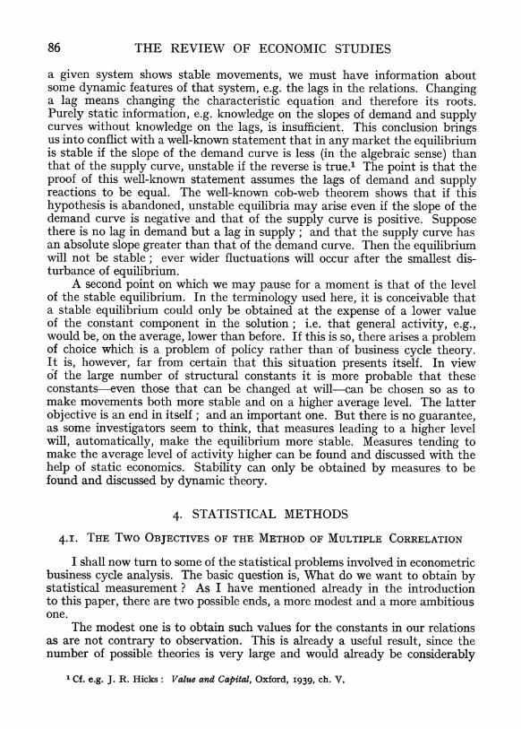
86 THE REVIEW OF ECONOMIC STUDIES
a given system shows stable movements, we must have information about some dynamic features of that system, e.g. the lags in the relations. Changing a lag means ch-anging the characteristic equation and therefore its roots. Purely static information, e.g. knowledge on the slopes of demand and supply curves without knowledge on the lags, is insufficient. This conclusion brings us into conflict with a well-known statement that in any market the equilibrium is stable if the slope of the demand curve is less (in the algebraic sense) than that of the supply curve, unstable if the reverse is true.1 The point is that the proof of this well-known statement assumes the lags of demand and supply reactions to be equal. The well-known cob-web theorem shows that if this hypothesis is abandoned, unstable equilibria may arise even if the slope of the demand curve is negative and that of the supply curve is positive. Suppose there is no lag in demand but a lag in supply; and that the supply curve has an absolute slope greater than that of the demand curve. Then the equilibrium will not be stable; ever wider fluctuations will occur after the smallest dis- turbance of equilibrium.
A second point on which we may pause for a moment is that of the level of the stable equilibrium. In the terminology used here, it is conceivable that a stable equilibrium could only be obtained at the expense of a lower value of the constant component in the solution; i.e. that general activity, e.g., would be, on the average, lower than before. If this is so, there arises a problem of choice which is a problem of policy rather than of business cycle theory. It is, however, far from certain that this situation presents itself. In view of the large number of structural constants it is more probable that these constants-even those that can be changed at will-can be chosen so as to make movements both more stable and on a higher average level. The latter objective is an end in itself; and an important one. But there is no guarantee, as some investigators seem to think, that measures leading to a higher level will, automatically, make the equilibrium more stable. Measures tending to make the average level of activity higher can be found and discussed with the help of static economics. Stability can only be obtained by measures to be found and discussed by dynamic theory.
4. STATISTICAL METHODS
4.I. THE Two OBJECTIVES OF THE METHOD OF MULTIPLE CORRELATION
I shall now turn to some of the statistical problems involved in econometric business cycle analysis. The basic question is, What do we want to obtain by statistical measurement ? As I have mentioned already in the introduction to this paper, there are two possible ends, a more modest and a more ambitious one.
The modest one is to obtain such values for the constants in our relations as are not contrary to observation. This is already a useful result, since the number of possible theories is very large and would already be considerably
1 Cf. e.g. J. R. Hicks: Value and Capital, Oxford, i939, ch. V.

ECONOMETRIC BUSINESS CYCLE RESEARCH 87
restricted by taking only such relations. The whole subject is so complicated that further theoretical treatment without choosing numerical values for a number of the coefficients would be waste of time. Various examples could be given of theories using unrealistic relations. The frequent use of the accelera- tion principle for the explanation of investment fluctuations is one. Not only is this principle a bad explanation of most forms of investment activity, but even in the cases where it fits the facts (railways) the coefficient usually assumed is not in agreemient with the facts.1
The first time I used multiple correlation analysis in business cycle theory 2
it was with this modest purpose in view. Afterwards the more ambitious objec- tive, to measure with some degree of exactness the values of the coefficients, came in. Various pitfalls in this field have recently been discussed and I need not repeat them here. I think the matter has been discussed fairly completely and that it is now more useful to apply the method to concrete cases. That there are cases where it has yielded results is, I think beyond question 3 and I hope to give some examples in ? 4.3. There are one or two remarks I want to make that have, perhaps, not yet sufficiently been emphasised.
One is of a very elementary character. We should not forget, while talking so much about the statistical significance and the standard deviations of our regression coefficients, that even if these standard deviations are large, the most probable value for the regression coefficient is the value we calculate. If no other information is available we can hardly avoid taking the regression co- efficient we find, however uncertain it may be.
4.2. OTHER METHODS
Another topic that may be considered somewhat more in detail is: are other methods available and what is their value ? First, we have what may be called the common-sense method of business cycle research, to be found in most periodic surveys of economic conditions.4 It consists in a careful cata- loguing of facts and of the month-to-month fluctuations in a number of relevant economic time series. In a number of cases it attributes, with a fairly high degree of plausibility, certain given changes to certain events and by so doing succeeds in explaining, to some degree, the mechanism of cyclical move- ments. I think the successful cases of explanation are those where in the series to be explained a sudden rather marked change occurs at the same time, or shortly after, some sudden change in another series, or some new event happens. Just because the changes are rather sudden ones, we have approximatively the situation that all other factors remain almost constant. Hence, in that short interval there is a simple correlation between the variable to be explained
1 Cf. J. Tinbergen: " Statistical Evidence on the Acceleration Principle," Economica V (I938), p. I64.
2 The first very elementary attempts are to be found in my " Survey on Quantitative Business Cycle Theory," Econometrica 3 (1935), pp. 284-6.
8 Even Mr. Keynes expresses this opinion (loc. cit.) notwithstanding the severity of his criticisms.
4 A very good piece of work in this category, written with great skill, is S. H. Slichter: " The Downturn of 1937," The Review of Economic Statistics, XX (1938), p. 97.

88 THE REVIEW OF ECONOMIC STUDIES
and the one explanatory variable that suddenly changes. It is evider this method can be successful especially for the analysing of the influence of new events, i.e. of the-often small-disturbances of the movements. To my mind it is, therefore, especially favoured by those who attribute to these new events a great role. It is far more difficult, if not impossible, to apply it to the ever-present factors that do not change suddenly. These have not the courtesy to wait with their changes until other things remain unchanged; and prevent us from playing that most beloved game of ceteris paribus. Looked at in this way, the common-sense method reduces to simple correlation analysis, applied to special cases.
There is another element in this common-sense method which has a methodological meaning in itself. This element is what I should like to call the experimental method of determining relations. Our relations often indicate how people would react if a certain change in prices, incomes, etc., were to occur. Instead of using multiple correlation analysis one might try an experiment, i.e. by some artificial means change only one factor at a time and see what people do. Large-scale and systematic experiments as in the natural sciences are, of course, excluded; but there are several forms of investigation that approximate to this method.
(i) One is the method of interview, described, e.g. by Mrs. Waterman- Gilboy and Frisch. Here we ask certain people what they would do in certain hypothetical circumstances. We could speak of a " virtual experiment." A counterpart of this method of interviewing is to ask people what was the reason for something they actually did.' This too, may, in principle, tell us something about the causes of a given change. It is this method that is fre- quently applied by common-sense business cycle research. The more informed the investigator is about the actual motives that have led people to react as they did, the better his approach will be.
(ii) There are other " experimental " investigations possible. In a sense, family budget statistics are an example. They tell us what the influence of income on expenditure is. Similar information may be obtained by comparing people living under different price situations, e.g. comparing the consumption of electricity in different localities; or comparing the ratio between labour and capital used in production in different countries. Data on cost curves for separate enterprises and on the distribution of enterprises over cost classes are a further important category in this class, which we may describe as " structural investigations."
We have now to compare the accuracy of these methods with that of multiple correlation analysis. This can hardly be done in one general statement. There are certainly cases where " experimental investigations " are much more reliable than correlation investigations. In particular, good " structural investigations " deserve much attention. But there are also many pitfalls here.
1 A splendid example is the Oxford inquiry on the factors influencing investment activity. Oxford Economic Papers, I (1938). For me, it is encouraging that this inquiry led to the same scepticism on the influence of the interest rate on investment activity as my investigation A Method and its Application to Investment Activity.

ECONOMETRIC BUSINESS CYCLE RESEARCH 89
Even a good family budget inquiry may be a bad guide if the distribution of income in the group considered does not fit with that in the country as a whole; or it may give a wrong expression of the relation in time between income and expenditure, since changes in time need not have the same consequences as changes from one income group to another. In particular, it is very difficult to know whether any structural investigation based on a sample is represen- tative.
The difficulties are considerably larger for the other types of " experi- mental investigations." The interview method, even if based on past events, must be somewhat superficial unless the utmost care is given to the formulation of questions-in order to make people conscious of what their own motives really have been. The way in which common-sense business cycle research uses this method is, in most cases, much more superficial still, since it is pri- marily based on newspaper information and personal opinions where even the best informed investigators only know a small part of the firms and individuals concerned. The way, moreover, in which accidental disturbances may influence the results of this type of explanation of fluctuations shows another danger of that method.
In conclusion, it would seem to me that the method of multiple correlation does not compare badly with the other methods. But we need not consider them as competitors. They can collaborate perfectly well. In most statistical determinations of demand curves I compared the results obtained-as far as the influence of income is concerned-with those of family budget investiga- tions. Dr. Polak has given a very interesting example of collaboration of the two methods in the explanation of the fluctuations in farm prices.'
4.3 RESULTS OF MULTIPLE CORRELATION ANALYSIS
Most critics of multiple correlation analysis admit that it may serve some purposes, as e.g. the determination of a demand function for some specific commodity. Hence the difference of opinion is about where the limits lie. As a first step in the fixation of the demarcation line let me sum up some cases where I think the method has given useful results. I do not claim any degree of completeness, however.
Apart from one or two scattered applications, published in the Journal of the Royal Statistical Society, soon after Mr. Yule's inauguration of the method, the pioneer work on economic applications has been done in the United States. Moore, Schultz, Ezekiel, Roos, Waugh and several others have made important contributions; the first three authors particularly in the field of agricultural economics. The random movements of crops favour the application of the method, since there is little correlation between prices of particular agricultural commodities and incomes. They succeeded in determining elasticities of demand and supply in a number of cases. Important work on non-farm markets was done by Roos and his assistants; especially in housing and in the automobile market.
1 In Business Cycles in the U,S,., section (3.4), which was entirely his work,
B3

go THE REVIEW OF ECONOMIC STUDIES
In Europe, Prof. Frisch and his followers (e.g. Haavelmo) have done much work in completing the method and applying it to demand studies for various consumers' goods. Part of Frisch's estimates of the marginal utility of income are based on multiple correlation analysis.
The German investigators Donner and Hanau have obtained several interesting results (cotton prices, German share prices; pig markets). Dr. H. Staehle has some very interesting (unpublished) investigations on the demand for labour in certain industries; further, in a discussion on the " pro- pensity to consume" he gave an interesting example of multiple correlation calculus.
Of the Dutch group I may mention T. Koopmans, who has considerably contributed to the development of the theory of the significance of regression coefficients, J. J. Polak, Derksen, De Wolff, Dalmulder, Rombouts, Mey, Smit, Van den Briel, Van der Schalk, and Van der Meer.' They and others have made numerous demand studies, not only for agricultural products, but also for industrial goods and services (e.g. motor cars, motor fuel, bicycles, postal services, tramway and railway traffic, electric current, cinema visits, shipping transport). In the League of Nations study (loc. cit.) the technique was, it seems to me, successfully applied to some new subjects as e.g. the monetary and banking sphere, the demand for investment goods and supply or price equations.
The Hague, Holland. J. TINBERGEN.
1 I apologise for mentioning so many compatriots and forgetting many more foreign investi- gators; the reason being that I want to draw the attention to work that is, for linguistic causes, not so well accessible to other than Dutch readers.