Embed Size (px)
Citation preview

The returns to undergraduate degrees by socio-economic group and ethnicity Research report
March 2021
Jack Britton, Lorraine Dearden and Ben Waltmann
Institute for Fiscal Studies

Executive summary
We investigate differences in the returns to undergraduate degrees by socio-economic background
and ethnicity using the Department for Education’s Longitudinal Education Outcomes (LEO) data
set. The LEO data set links school records, university records and tax records for everyone w ho
took GCSEs in England since 2002. Using these data, we can estimate returns up to age 30. Our
main findings are:
• Average returns to undergraduate degrees at age 30 are positive for people from all socio-
economic and ethnic groups we study, but there is substantial heterogeneity across groups.
Returns are especially high for privately-educated graduates, whose median earnings at age
30 are the highest of all groups. However, we find that the groups with the lowest graduate
earnings, such as Pakistani students or state-educated students from the poorest families,
also have relatively high returns from going to university. The reason is that the earnings
prospects of these groups are very low on average if they do not attend university.
• Besides high returns for privately educated students, returns vary relatively little by
socio-economic status. At age 30, we find gross earnings returns of around 6% for state-
educated men and around 27% for state-educated women. If anything, returns are some-
what higher for state-educated students from the poorest 20% of families, with returns at
around 7% for men and 31% for women. Returns for privately educated students are much
higher at around 29% for men and 36% for women.
• By ethnicity, we see especially high returns for South Asian students. In particular, we
find returns of 27% for Indian women, 40% for Pakistani women and 30% for Bangladeshi
women, as well as 16% for Indian men, 36% for Pakistani men and 14% for Bangladeshi men.
Strikingly, Pakistani graduates have the highest returns of all ethnic groups, even though
they have the lowest median age-30 earnings at £23,000 for men and £19,000 for women.
• Returns for Black women are somewhat lower than for White British women. Estimated
returns are 9% for Black Caribbean women, 20% for Black African women and 23% for Other
Black women, compared with 28% for White British women. For Black men, estimated re-
turns differ widely between different subgroups: returns for Black African men are large at
15%, but returns for Black Caribbean men are similar to returns for White British men at 7%,
and returns for Other Black men are low at 4%.
2
• Some but not all of the differences in returns can be explained by variation in subjects
chosen and institutions attended. Subject choice explains little of the variation in returns
by socio-economic status, but a substantial amount of the variation in returns by ethnicity:
Asian students systematically choose more lucrative subjects than White British students.
Conversely, institution choices can partly explain why private school students get higher
returns from university than those who attended state schools; however, institution choices
do not explain much of the variation in returns by ethnicity.
• Unexplained differences in earnings between groups are mostly smaller among graduates
than among non-graduates. This implies that differences in the returns to higher education
‘even out’ some of the earnings differences between non-graduates that cannot be explained
by other factors. However, large unexplained earnings gaps between socio-economic and
ethnic groups remain. In particular, controlling for background conditions, prior attainment,
and university and subject choice, graduate men from all non-White ethnic groups earn
significantly less than White British graduates.
We supplement these age-30 results with estimated discounted net lifetime returns in pounds for
the different groups based on a simulation of lifetime earnings. This simulation is subject to a large
amount of uncertainty, so the results should be treated with caution. We account for the effect of
the tax and student loans system and we discount using Treasury Green Book discounting. The
main results are:
• Lifetime returns by socio-economic status follow a U shape. For women, the average re-
turn varies between £140,000 for the bottom quintile and £70,000 for the top state quintile.
For men, the returns are similar to the estimates for women for the bottom four SES quintiles,
but higher at around £110,000 for the top state SES quintile, while for the privately educated
the returns are much higher at around £250,000.
• Lifetime returns by ethnicity follow a similar pattern to gross returns at age 30. Returns
for South Asian students are relatively high at around £200,000 for men and around £170,000
for women. Estimated returns for Black students are relatively low at around £50,000; an
exception is Black African women, for whom we estimate a lifetime return of £175,000 on
average. White British, White Other, and Other students have middling returns of roughly
£100,000 for both men and women.
3

Contents
1 Introduction 8
2 Data 11
2.1 Overview . . . . . . . . . . . . . . . . . . . . . . . . . . . . . . . . . . . . . . . . . . . . 11
2.2 Measures of SES and ethnicity . . . . . . . . . . . . . . . . . . . . . . . . . . . . . . . . 12
2.3 Undergraduate participation . . . . . . . . . . . . . . . . . . . . . . . . . . . . . . . . 14
3 Differences between socio-economic and ethnic groups 16
3.1 Earnings at age 30 . . . . . . . . . . . . . . . . . . . . . . . . . . . . . . . . . . . . . . . 17
3.2 Prior attainment . . . . . . . . . . . . . . . . . . . . . . . . . . . . . . . . . . . . . . . . 22
3.3 Location . . . . . . . . . . . . . . . . . . . . . . . . . . . . . . . . . . . . . . . . . . . . 24
3.4 Universities attended . . . . . . . . . . . . . . . . . . . . . . . . . . . . . . . . . . . . . 26
3.5 Subjects studied . . . . . . . . . . . . . . . . . . . . . . . . . . . . . . . . . . . . . . . . 29
4 Methodology 31
4.1 Estimating earnings returns at age 30 . . . . . . . . . . . . . . . . . . . . . . . . . . . . 32
4.2 Simulating lifetime earnings . . . . . . . . . . . . . . . . . . . . . . . . . . . . . . . . . 33
4.3 Estimating lifetime returns . . . . . . . . . . . . . . . . . . . . . . . . . . . . . . . . . . 33
5 Early-career returns 34
5.1 Gross returns at age 30 . . . . . . . . . . . . . . . . . . . . . . . . . . . . . . . . . . . . 34
5.2 Importance of institution and subject choices in age-30 returns . . . . . . . . . . . . . 38
5.3 Unexplained differences in earnings . . . . . . . . . . . . . . . . . . . . . . . . . . . . 41
6 Lifetime earnings 44
6.1 Lifetime earnings simulations . . . . . . . . . . . . . . . . . . . . . . . . . . . . . . . . 45
6.2 Gross returns at older ages . . . . . . . . . . . . . . . . . . . . . . . . . . . . . . . . . . 47
6.3 Lifetime returns . . . . . . . . . . . . . . . . . . . . . . . . . . . . . . . . . . . . . . . . 49
7 Conclusion 54
Bibliography 56
4

A1 Robustness: using IDACI instead of our SES measure 58
A2 Gender earnings gaps 59
A3 University subject choice by gender 62
A4 Age 30: unexplained gaps in earnings by SES and ethnicity 66
A5 Age 30 returns: graphs 68
Acknowledgements
The authors would like to thank the Department for Education for providing access to data and
helping to develop this report and Judith Payne for outstanding copy-editing. They are grateful
to the Economic and Social Research Council (grant ES/S010718/1) and the ESRC Centre for the
Microeconomic Analysis of Public Policy (grant ES/T014334/1) for funding.
5

List of Figures
1 HE participation by SES . . . . . . . . . . . . . . . . . . . . . . . . . . . . . . . . . . . 15
2 HE participation by ethnicity . . . . . . . . . . . . . . . . . . . . . . . . . . . . . . . . 16
3 Median age-30 earnings of women by socio-economic group . . . . . . . . . . . . . . 17
4 Median age-30 earnings of men by socio-economic group . . . . . . . . . . . . . . . . 18
5 Median age-30 earnings of women by ethnicity . . . . . . . . . . . . . . . . . . . . . . 19
6 Median age-30 earnings of men by ethnicity . . . . . . . . . . . . . . . . . . . . . . . . 20
7 Median GCSE percentile by SES and HE attendance . . . . . . . . . . . . . . . . . . . 23
8 Median GCSE percentile by ethnicity and HE attendance . . . . . . . . . . . . . . . . 24
9 Socio-economic status: distribution across regions . . . . . . . . . . . . . . . . . . . . 25
10 Ethnicity: distribution across regions . . . . . . . . . . . . . . . . . . . . . . . . . . . . 26
11 Distribution across institutions by SES . . . . . . . . . . . . . . . . . . . . . . . . . . . 27
12 Distribution across institutions by ethnicity . . . . . . . . . . . . . . . . . . . . . . . . 28
13 Subject choices by SES relative to average . . . . . . . . . . . . . . . . . . . . . . . . . 29
14 Subject choices by ethnicity relative to White British . . . . . . . . . . . . . . . . . . . 31
15 Unexplained earnings gaps between SES groups: HE and non-HE . . . . . . . . . . . 42
16 Unexplained earnings gaps between ethnic groups: HE and non-HE . . . . . . . . . 43
17 Predicted net lifetime earnings by SES . . . . . . . . . . . . . . . . . . . . . . . . . . . 45
18 Predicted net lifetime earnings by ethnicity . . . . . . . . . . . . . . . . . . . . . . . . 47
19 Gross returns at older ages by SES . . . . . . . . . . . . . . . . . . . . . . . . . . . . . 48
20 Gross returns at older ages by ethnicity . . . . . . . . . . . . . . . . . . . . . . . . . . 49
21 Predicted net lifetime returns by SES . . . . . . . . . . . . . . . . . . . . . . . . . . . . 50
22 Share with positive lifetime returns by SES . . . . . . . . . . . . . . . . . . . . . . . . 51
23 Predicted net lifetime returns by ethnicity . . . . . . . . . . . . . . . . . . . . . . . . . 52
24 Share with positive lifetime returns by ethnicity . . . . . . . . . . . . . . . . . . . . . 54
A1 Median age-30 gender earnings gap by socio-economic status . . . . . . . . . . . . . 59
A2 Median age-30 gender earnings gap by ethnicity . . . . . . . . . . . . . . . . . . . . . 60
A3 Decomposition of the overall graduate gender earnings gap (in %) . . . . . . . . . . 61
A4 Subject choices by SES relative to average, women . . . . . . . . . . . . . . . . . . . . 62
6

A5 Subject choices by SES relative to average, men . . . . . . . . . . . . . . . . . . . . . . 63
A6 Subject choices by ethnicity relative to White British, women . . . . . . . . . . . . . . 64
A7 Subject choices by ethnicity relative to White British, men . . . . . . . . . . . . . . . . 65
A8 Returns by SES: successive controls . . . . . . . . . . . . . . . . . . . . . . . . . . . . . 68
A9 Returns by ethnicity: successive controls . . . . . . . . . . . . . . . . . . . . . . . . . . 69
A10 Returns by SES: impact of subject and institution choice, relative to highest SES
quintile . . . . . . . . . . . . . . . . . . . . . . . . . . . . . . . . . . . . . . . . . . . . . 70
A11 Returns by ethnicity: impact of subject and institution choice, relative to White British 71
List of Tables
1 Sample size by SES and GCSE year . . . . . . . . . . . . . . . . . . . . . . . . . . . . . 12
2 Sample size by ethnicity and GCSE year . . . . . . . . . . . . . . . . . . . . . . . . . . 13
3 Sample size by ethnicity and SES group . . . . . . . . . . . . . . . . . . . . . . . . . . 14
4 Median age-30 earnings by SES and ethnicity . . . . . . . . . . . . . . . . . . . . . . . 21
5 Age-30 returns by SES . . . . . . . . . . . . . . . . . . . . . . . . . . . . . . . . . . . . 35
6 Age-30 returns by ethnicity . . . . . . . . . . . . . . . . . . . . . . . . . . . . . . . . . 37
7 Impact of subject and institution on relative returns by SES . . . . . . . . . . . . . . . 39
8 Impact of subject and institution on relative returns by ethnicity . . . . . . . . . . . . 40
A1 Sample size by SES and IDACI . . . . . . . . . . . . . . . . . . . . . . . . . . . . . . . 58
A2 Age-30 returns by IDACI . . . . . . . . . . . . . . . . . . . . . . . . . . . . . . . . . . . 58
A3 Unexplained gaps in earnings by socio-economic status: age 30 . . . . . . . . . . . . 66
A4 Unexplained gaps in earnings by ethnicity: age 30 . . . . . . . . . . . . . . . . . . . . 67
7

1 Introduction
For several decades, a major aim of educational policy in the UK has been to improve outcomes
for children born into more disadvantaged circumstances. Improving access to higher education
for disadvantaged students has been a key element in achieving this. Despite some progress – the
proportion of students from low-participation neighbourhoods has almost doubled since 2006 –
participation gaps between rich and poor students remain large: nearly half of young people from
the most advantaged quintile of neighbourhoods secured a place in undergraduate university
courses in 2018 compared with only one-fifth of students from the most deprived quintile.1 There
are also large differences in university attendance by ethnicity: White British students have the
lowest participation rates, while Indian and Chinese students have the highest (Crawford and
Greaves, 2015).
While there is a large literature that documents gaps in access to higher education between
different groups and investigates ways to reduce them2 and an equally large literature investigat-
ing overall returns to higher education,3 there is much less evidence investigating how returns
to higher education vary by socio-economic background and ethnicity.4 This is a shortfall of the
literature, as evidence on this question is important for policy. Work on this question could help
explain participation gaps while also highlighting the role higher education could play in reducing
inequality.
Recent data developments in the UK have enabled some studies to revisit the question of
the returns to higher education, drawing on linked administrative records that contain detailed
information on the prior attainment and background of each individual student and their earnings
records. Belfield et al. (2018) use these data to investigate gross earnings returns at an early stage
of graduates’ careers (roughly, age 29), while Britton et al. (2020) estimate the lifetime returns
to higher education. Both of these reports primarily focus on how returns vary by institution
1This is based on ‘POLAR’, which is a less refined measure of deprivation than we have available. See UCAS (2018).2For example, see Chowdry et al. (2013), Crawford, Dearden and Greaves (2014) and Crawford and Greaves (2015)
in the UK and Hoxby and Avery (2013) and Dynarski et al. (2018) in the US.3See Altonji, Blom and Meghir (2012) for a review and Walker and Zhu (2011), Walker and Zhu (2018), Belfield et al.
(2018) and Britton et al. (2020) for evidence from the UK.4Arcidiacono and Lovenheim (2016) provide a review of the returns to higher education for ethnic minorities, draw-
ing on evidence from affirmative action policies; Zimmerman (2019) compares returns to elite college access for richand poor students; Chetty et al. (2017) compare earnings outcomes for rich and poor students the US; Britton et al.(2019) compare outcomes conditional on subject and institution for richer and poorer students in the UK.
8

attended and subject studied, rather than on how they vary by background characteristics of the
students. In this report, we make use of the same linked administrative records – referred to as
the ‘Longitudinal Education Outcomes’ (LEO) data set – and expand upon these previous studies
by focusing on returns to higher education by age-16 socio-economic status (SES) and ethnicity.
For our measure of SES, we follow several recent studies (e.g. Chowdry et al., 2013) and create a
continuous index of deprivation based on a combination of individual characteristics and various
measures of deprivation of the local area people live in when they are aged 16. We divide people
into five quintiles based on this index, and also create a sixth group who were educated outside of
the state system – we typically think of this group as being the most advantaged, as the majority
attended fee-paying independent schools. For ethnicity, we use fairly coarse categories that are
available from the National Pupil Database.5
We start by documenting differences in participation between our different groups. Our focus
is on people who took their GCSE examinations between 2002 and 2007, as these are the individu-
als for whom we have information on their earnings outcomes. Individuals in these cohorts who
went to university will typically have entered university between 2004 and 2010, and graduated
between 2007 and 2013. Like the previous literature, we find large gaps in higher education (HE)
participation between richer and poorer students and between White and Asian students.
We then move on to investigate earnings outcomes. For both women and men, median earn-
ings at age 30 rise with socio-economic background. This is true both among those who attended
university and those who did not (one exception is privately educated men who did not attend
university, whose median earnings are lower than those of people from the top two quintiles of
state-educated students who did not attend university.) For ethnicity, the picture is more nuanced
but, broadly speaking, Chinese, Indian and White people have the highest median earnings and
Pakistani, Black Caribbean and Bangladeshi people the lowest. Apart from differences in HE
participation, possible explanations for these patterns include differences in prior attainment, lo-
cation, university choices and subject choices. We show that all of these factors vary considerably
across our subgroups.
In order to isolate differences in returns from differences in prior attainment, location and other
5Specifically, these are White British, White Other, Black African, Black Caribbean, Black Other, Bangladeshi, Chi-nese, Indian, Pakistani and Other.
9

confounding factors, we estimate similar models to those in Belfield et al. (2018). We find gross
earnings returns at age 30 of around 6% for state-educated men and around 27% for state-educated
women; only the bottom quintile of women achieve somewhat higher returns, at around 31%. For
both women and men, returns for the privately educated are higher – at around 36% for women
and around 29% for men. By ethnicity, we find very large returns for South Asian students and
somewhat lower returns for Black women.
We then investigate the extent to which differences in returns estimates are affected by subject
and institution choices between those coming from different SES backgrounds and those in differ-
ent ethnicity groups. Our findings suggest that among state-educated students, those from higher
SES backgrounds typically make worse subject choices in terms of earnings potential. Those from
lower SES groups are much more likely to choose law, computing or business, all of which yield
relatively good returns on average. The opposite is true for university choices, however, with the
lowest SES groups making the worst choices in terms of earnings returns, even taking into account
differences in prior attainment.
By ethnicity, it appears that Asian and Black African students make by far the best subject
choices in terms of maximising earnings potential, with a very high propensity to choose voca-
tional subjects such as business, computing, law and pharmacology. Students from other eth-
nicities have higher propensities to choose lower-returning subjects such as sociology, creative
arts and social care. Institution choices play a fairly minor role in driving differences in returns
between ethnicities, although there is some evidence suggesting that Asian students also make
institution choices that improve earnings prospects.
We show that remaining differences in returns to a large extent mirror unexplained differ-
ences in earnings between groups for non-graduates. As a result, unexplained differences be-
tween groups are smaller among graduates. However, remaining unexplained differences among
graduates are still statistically and economically significant.
Finally, we simulate the lifetime earnings of young people to estimate what returns to higher
education are likely to look like at later ages than we can observe in the LEO data set. We show
that returns are likely to grow with age for all groups, and especially for men. We then use our
simulated earnings model to estimate the discounted net present value of lifetime returns to at-
10

tending higher education, taking into account both taxes and student loan repayments.6 We find a
U shape in returns by socio-economic background, with the lowest SES groups and independent
school students benefiting most from higher education over their lifetimes. By ethnicity, South
Asian students (in particular, Pakistani students) benefit the most from higher education over the
course of their lifetimes, while Black students tend to benefit the least.
The report is laid out as follows. Section 2 describes the data set we use and Section 3 doc-
uments relevant differences between socio-economic and ethnic groups. Section 4 discusses the
methodology for estimating returns and simulating lifetime earnings. Section 5 then estimates
gross returns at age 30 and investigates the importance of subject and institution choices, and
Section 6 shows our lifetime estimates. Section 7 concludes.
2 Data
2.1 Overview
We briefly summarise the data that we use, referring the reader to Britton et al. (2020) for more
extensive detail. We use the Longitudinal Education Outcomes (LEO) data set, an administrative
data set that links together school records from the National Pupil Database (NPD), university
records from the Higher Education Statistics Agency (HESA) and tax records from Her Majesty’s
Revenue and Customs (HMRC). We focus on students who took their GCSE examinations in Eng-
land between 2002 and 2007. The 2002 GCSE cohort is the oldest cohort for which we have linked
NPD–HESA–HMRC data, and we observe those individuals in the tax data up to age 30. In our
returns estimates, we focus on those who attained at least five GCSEs graded A*–C, for whom
higher education was a plausible option.
For our lifetime returns estimates, we concentrate on the 2002 cohort only. As laid out in more
detail in the methodology section, after age 30 we simulate earnings for everyone in the 2002
cohort with five A*–C GCSEs and a Key Stage 5 record for the rest of their working lives. For
this exercise, we use two different data sources. The first is the linked HESA–HMRC record for
cohorts of students born between the mid 1970s and the mid 1980s. This gives us linked individual
earnings records over time for university students back to the 1975/76 birth cohort (for this oldest
6Our methodology for this exercise closely follows Britton et al. (2020).
11

cohort, we observe earnings up to age 40). The second is the Labour Force Survey (LFS), which
we use to simulate earnings from ages 41 to 67 for university students and from ages 31 to 67 for
the non-university group (as we do not have the HMRC data up to age 40 for the latter).
2.2 Measures of SES and ethnicity
Unfortunately, we do not observe parental income. However, following previous research in this
area (e.g. Chowdry et al., 2013) and our own previous work with the LEO data (e.g. Belfield et al.,
2018), we generate a continuous measure of SES based on a combination of the free school meals
(FSM) indicator and a set of local area deprivation measures. We combine these variables into one
continuous measure using principal components analysis and then divide it up into quintiles that
range from most deprived to least deprived.7 We do not observe the local-area-level deprivation
index for the roughly 8% of students who attended private schools – we therefore include them as
a sixth and separate group.
Table 1: Sample size by SES and GCSE yearSES group 2002 2003 2004 2005 2006 2007 Total
Bottom quintile 90,162 98,354 108,284 107,992 100,269 102,677 607,7382nd quintile 93,902 102,645 109,960 109,576 105,618 107,522 629,2233rd quintile 97,001 105,851 111,692 111,231 109,940 111,298 647,0134th quintile 98,483 108,148 112,859 112,416 112,379 114,049 658,334Top quintile 99,287 109,206 113,340 113,053 113,859 115,407 664,152Independent school 40,888 40,773 43,745 46,095 46,651 47,199 265,351Total 519,723 564,977 599,880 600,363 588,716 598,152 3,471,811
Note: Differences in quintile size arise because lower-SES students are more likely to have incomplete Key Stage 4records.
Table 1 shows the number of individuals in our sample by SES group and GCSE year. We ob-
serve around half a million individuals per GCSE cohort and 3.5 million individuals overall. Small
differences in quintile size arise because lower-SES students are more likely to have incomplete
Key Stage 4 records and we have excluded those with incomplete records from the sample.
We use ethnicity information from the NPD. The categories we use are: White British, White
Other, Black African, Black Caribbean, Black Other, Bangladeshi, Chinese, Indian, Pakistani and
Other. Ethnicity is not available for those who were not state educated; hence, our returns esti-
7As shown in Appendix A1, our composite SES index is highly correlated with the Income Deprivation AffectingChildren Index (IDACI), and we obtain very similar results when we use the IDACI quintile instead.
12

mates by ethnicity should be interpreted as applying only to students educated in the state school
system.
Table 2: Sample size by ethnicity and GCSE yearEthnicity 2002 2003 2004 2005 2006 2007 Total
White British 397,124 419,684 452,513 451,025 443,074 451,216 2,614,636White Other 11,544 9,062 10,292 10,304 10,620 11,251 63,073Black Caribbean 6,653 7,545 8,068 8,167 7,750 7,603 45,786Black African 5,915 6,828 7,674 8,914 9,412 10,214 48,957Black Other 3,635 2,107 2,296 2,320 2,373 2,383 15,114Indian 12,824 13,257 13,458 12,728 12,889 12,694 77,850Pakistani 12,113 12,048 12,799 12,615 12,722 13,305 75,602Bangladeshi 4,489 4,836 4,981 5,043 5,356 5,279 29,984Chinese 1,770 1,815 1,897 2,141 1,992 1,931 11,546Other 22,768 47,022 42,157 41,011 35,877 35,077 223,912Total 478,835 524,204 556,135 554,268 542,065 550,953 3,206,460
Note: Excludes privately educated students.
Table 2 shows the number of individuals in our sample by ethnic group and GCSE year. As
privately educated students are excluded, the overall sample size is somewhat smaller, at 3.2 mil-
lion. Notably, the vast majority of students are classified as White British, while Chinese and Black
Other each describe fewer than 20,000 students. It should also be noted that the ethnicity classifi-
cations in the NPD became more refined over time, with smaller and mixed ethnicities explicitly
included in later years; as a result, ethnicity categories are not precisely identical in different co-
horts.8
Table 3 cross-tabulates sample sizes between ethnic groups and socio-economic status quin-
tiles. Ethnic diversity decreases in higher SES quintiles. Some ethnic minorities, such as Black
African and Bangladeshi, are vastly over-represented in the lowest socio-economic group. Others,
such as White Other and Chinese, are more evenly split.
8Most significantly, changes in ethnicity coding appear to have led to a large rise between the 2002 and 2003 cohortsin students classified as ‘Other’ in our classification scheme, as students who would otherwise have been classed undera single ethnicity were now classified as mixed and therefore fell under ‘Other’.
13
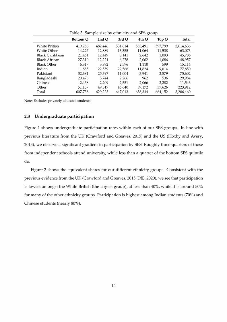
Table 3: Sample size by ethnicity and SES groupBottom Q 2nd Q 3rd Q 4th Q Top Q Total
White British 419,286 482,446 531,614 583,491 597,799 2,614,636White Other 14,227 12,889 13,355 11,064 11,538 63,073Black Caribbean 21,461 12,449 8,141 2,642 1,093 45,786Black African 27,310 12,221 6,278 2,062 1,086 48,957Black Other 6,817 3,992 2,596 1,110 599 15,114Indian 11,885 22,559 22,568 11,824 9,014 77,850Pakistani 32,681 25,397 11,004 3,941 2,579 75,602Bangladeshi 20,476 5,744 2,266 962 536 29,984Chinese 2,438 2,209 2,551 2,066 2,282 11,546Other 51,157 49,317 46,640 39,172 37,626 223,912Total 607,738 629,223 647,013 658,334 664,152 3,206,460
Note: Excludes privately educated students.
2.3 Undergraduate participation
Figure 1 shows undergraduate participation rates within each of our SES groups. In line with
previous literature from the UK (Crawford and Greaves, 2015) and the US (Hoxby and Avery,
2013), we observe a significant gradient in participation by SES. Roughly three-quarters of those
from independent schools attend university, while less than a quarter of the bottom SES quintile
do.
Figure 2 shows the equivalent shares for our different ethnicity groups. Consistent with the
previous evidence from the UK (Crawford and Greaves, 2015; DfE, 2020), we see that participation
is lowest amongst the White British (the largest group), at less than 40%, while it is around 50%
for many of the other ethnicity groups. Participation is highest among Indian students (70%) and
Chinese students (nearly 80%).
14

Figure 1: HE participation by SES
0 20 40 60 80 100percent
Indep. School
Top Quintile
4th Quintile
3rd Quintile
2nd Quintile
Bottom Quintile
HE no HE
Note: Quintiles refer to the distribution of socio-economic status among the state-educated. Includes data from the2002 to 2007 GCSE groups. Only those who have studied on standard undergraduate degrees are counted in the HEgroup. Students who have pursued sub-degree qualifications are counted as ‘non-HE’, and those recorded in the dataas pursuing postgraduate but not undergraduate qualifications are excluded from the sample.
15

Figure 2: HE participation by ethnicity
0 20 40 60 80 100percent
Chinese
Indian
Black African
Pakistani
White Other
Bangladeshi
Black Other
Black Caribbean
Other
White British
HE no HE
Note: Includes data from the 2002 to 2007 GCSE groups for people who attended state school only; people who attendedindependent schools are excluded from the sample, as their ethnicity is not recorded in most cases. Only those whohave studied on standard undergraduate degrees are counted in the HE group. Students who have pursued sub-degreequalifications are counted as ‘non-HE’, and those recorded in the data as pursuing postgraduate but not undergraduatequalifications are excluded from the sample.
3 Differences between socio-economic and ethnic groups
In this section, we first document differences in earnings at age 30 between socio-economic and
ethnic groups for men and women and for graduates and non-graduates. We then look at some
of the factors that could explain the observed earnings differences. Socio-economic and ethnic
groups differ in their school attainment and their regional concentration, which may drive dif-
ferences in earnings. Furthermore, people from different groups who go to university also make
different choices about where and what to study, which also influence their later-life earnings.
16

3.1 Earnings at age 30
Figure 3: Median age-30 earnings of women by socio-economic group
05
1015
2025
3035
Med
ian
Pre
-Tax
Ear
ning
s A
ge 3
0
Bottom
Quin
tile
2nd Q
uintile
3rd Q
uintile
4th Q
uintile
Top Q
uintile
Indep
. Sch
ool
HE non-HE Overall
Note: Median earnings from employment and self-employment for women from the 2002 GCSE cohort at age 30(2016/17 tax year) by socio-economic group, in thousands of pounds. Excludes individuals with zero or negativeearnings.
Figure 3 shows the median earnings at age 30 for women from the 2002 GCSE cohort by socio-
economic group. There is a clear gradient with socio-economic status for both HE and non-HE
women: women from wealthier backgrounds generally earn more. As more women from higher-
status groups attend university, the overall gradient in median earnings is steeper than the gradi-
ent for the HE and non-HE groups taken individually.
17

Figure 4: Median age-30 earnings of men by socio-economic group0
510
1520
2530
35M
edia
n P
re-T
ax E
arni
ngs
Age
30
Bottom
Quin
tile
2nd Q
uintile
3rd Q
uintile
4th Q
uintile
Top Q
uintile
Indep
. Sch
ool
HE non-HE Overall
Note: Median earnings from employment and self-employment for men from the 2002 GCSE cohort at age 30 (2016/17tax year) by socio-economic group, in thousands of pounds. Excludes individuals with zero or negative earnings.
Figure 4 is the equivalent graph for men. It shows a similar pattern, although the difference
in median earnings between the HE and non-HE groups is much smaller for men. An exception
is men who went to private schools: for privately educated men who did not go to university,
median earnings are actually lower than for state-educated high-SES men who did not attend uni-
versity. As a result, the gap between the HE and non-HE groups is much larger for privately
educated men than for state-educated men.
Notably, men in all groups have substantially higher median earnings at age 30 than women in
the same group. As shown in Figure A1 in the appendix, gender earnings gaps are larger between
non-HE men and women than between HE men and women within all socio-economic groups
except independent school students. The overall gender earnings gap falls with socio-economic
status, but the earnings gap among the HE group rises with socio-economic status.
18

Figure 5: Median age-30 earnings of women by ethnicity0
510
1520
2530
35M
edia
n P
re-T
ax E
arni
ngs
Age
30
Pakist
ani
Black C
aribb
ean
Bangla
desh
i
Black O
ther
Whit
e Briti
shOthe
r
Black A
frican
Whit
e Othe
r
Indian
Chines
e
HE non-HE Overall
Note: Median earnings from employment and self-employment for women from the 2002 GCSE cohort at age 30(2016/17 tax year) by ethnicity, in thousands of pounds. Excludes individuals with zero or negative earnings andthose who were privately educated.
Figure 5 shows the median earnings at age 30 for women from the 2002 GCSE cohort by ethnic
group. Pakistani, Black Caribbean and Bangladeshi women have the lowest median earnings at
age 30, at just above £15,000; at the other end of the spectrum, the median income of Indian and
Chinese women at age 30 is more than £25,000. By far the largest ethnic group, White British, has
median earnings of around £18,000.
Figure 6 is the equivalent graph for men. The ordering is very similar, with Pakistani, Black
Caribbean and Bangladeshi at the low end and Indian and Chinese at the high end of the spectrum.
Notably, among those who do not go to university, Indian and Chinese men actually have lower
earnings than White British men, and those who go to university have roughly the same median
earnings. Overall median earnings for Indian and Chinese men are higher only because a higher
19

Figure 6: Median age-30 earnings of men by ethnicity0
510
1520
2530
35M
edia
n P
re-T
ax E
arni
ngs
Age
30
Pakist
ani
Black C
aribb
ean
Bangla
desh
i
Black O
ther
Black A
frican
Other
Whit
e Briti
sh
Whit
e Othe
r
Indian
Chines
e
HE non-HE Overall
Note: Median earnings from employment and self-employment for men from the 2002 GCSE cohort at age 30 (2016/17tax year) by ethnicity, in thousands of pounds. Excludes individuals with zero or negative earnings and those whowere privately educated.
share of them attend university.
As shown in Figure A2 in the appendix, gender earnings gaps are larger among White British
people than among all minority groups. Black African, Chinese and Indian are the ethnic groups
with the smallest gender earnings gaps. Interestingly, for ethnic Indians, Pakistanis and Bangladeshis,
gender earnings gaps are larger among the HE group than among the non-HE group, reversing
the usual pattern.
20

Table 4: Median age-30 earnings by SES and ethnicityBottom Q 2nd Q 3rd Q 4th Q Top Q
Women
White British 12,661 15,133 17,764 19,863 23,116(21,896) (26,887) (31,231) (34,852) (36,349)
White Other 16,629 17,845 22,169 22,177 27,040(796) (831) (899) (853) (894)
Black Caribbean 15,475 16,731 19,061 15,660 23,232(1,249) (695) (427) (135) (58)
Black African 19,902 20,374 25,115 22,188 23,478(1,096) (480) (251) (75) (46)
Black Other 13,422 18,314 19,656 21,382 20,870(590) (363) (225) (124) (61)
Indian 20,757 23,165 26,625 27,652 28,524(793) (1,464) (1,448) (739) (539)
Pakistani 13,677 15,531 17,325 17,889 20,412(1,547) (1,269) (558) (184) (120)
Bangladeshi 15,784 17,098 21,271 18,855 .(931) (251) (96) (56) (17)
Chinese 25,479 23,960 24,046 27,724 30,667(144) (111) (145) (110) (123)
Other 15,839 17,153 19,556 21,303 23,893(1,652) (1,756) (1,683) (1,605) (1,674)
Men
White British 21,294 23,309 25,522 27,420 29,813(23,815) (29,247) (34,312) (37,965) (39,071)
White Other 22,232 24,749 26,968 28,576 31,820(926) (869) (944) (872) (897)
Black Caribbean 18,560 20,777 22,248 23,546 25,120(1,136) (632) (439) (145) (54)
Black African 21,320 23,078 23,768 25,993 26,365(943) (472) (221) (84) (47)
Black Other 19,895 23,168 24,114 22,663 26,557(548) (332) (222) (94) (53)
Indian 24,527 25,272 30,336 31,529 31,551(881) (1,650) (1,583) (808) (564)
Pakistani 16,440 19,695 21,321 21,747 25,937(2,002) (1,554) (680) (206) (131)
Bangladeshi 20,247 20,897 22,403 28,187 25,262(1,125) (306) (109) (41) (32)
Chinese 27,600 28,323 28,998 30,188 24,642(150) (136) (133) (130) (115)
Other 21,593 23,056 25,306 26,635 29,604(1,757) (1,816) (1,784) (1,681) (1,731)
Note: Median earnings from employment and self-employment in pounds for students from the 2002 GCSE cohort atage 30 (2016/17 tax year) by SES group and ethnicity. Excludes individuals with zero or negative earnings, and thosewho were privately educated. Sample sizes are shown in parentheses. ‘.’ indicates excluded to guard against statisticaldisclosure.
21

Table 4 shows median earnings of women and men by ethnic group and socio-economic sta-
tus. Within each ethnic group, higher socio-economic status is generally associated with higher
median earnings at age 30. Exceptions are Indian, Bangladeshi and Chinese men in the highest
SES cohorts. Comparatively low earnings for these groups may be explained by a high prevalence
of postgraduate study and therefore delayed labour market entry.
Within each socio-economic group, women from ethnic minorities tend to outearn their White
British peers. For men, the picture is more mixed, with Chinese and Indian men mostly earning
more than White British men with the same socio-economic background and men from other
ethnic minorities mostly earning less. In line with the overall results, ethnic Chinese and Indian
women also tend to be the highest earners within each SES group.
3.2 Prior attainment
We now consider one potential driver of these differences: prior attainment. We show the median
GCSE percentile rank by SES in Figure 7 and by ethnicity in Figure 8. In both cases, differences
in prior attainment align quite closely with differences in age-30 earnings, suggesting that prior
attainment could be a major factor in explaining differences between groups.
22
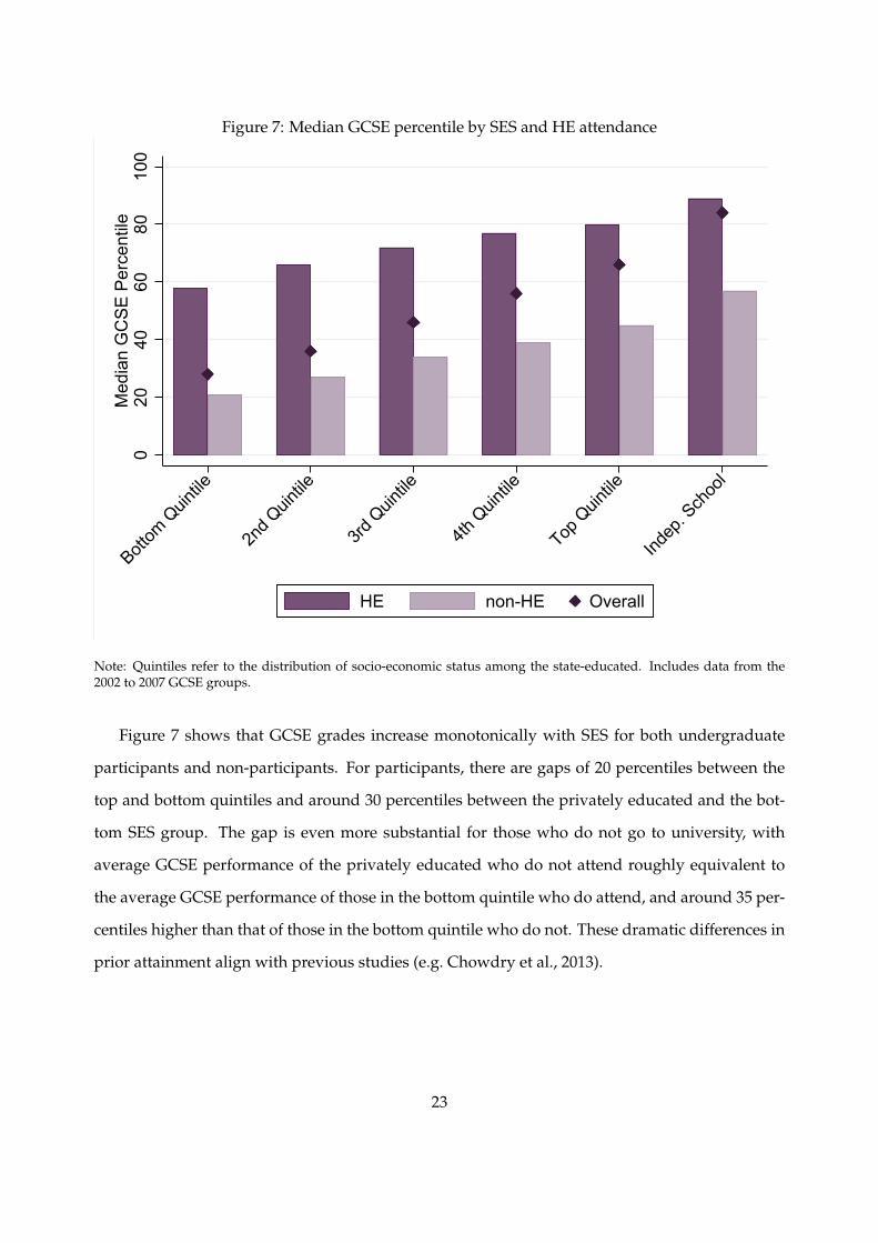
Figure 7: Median GCSE percentile by SES and HE attendance0
2040
6080
100
Med
ian
GC
SE
Per
cent
ile
Bottom
Quin
tile
2nd Q
uintile
3rd Q
uintile
4th Q
uintile
Top Q
uintile
Indep
. Sch
ool
HE non-HE Overall
Note: Quintiles refer to the distribution of socio-economic status among the state-educated. Includes data from the2002 to 2007 GCSE groups.
Figure 7 shows that GCSE grades increase monotonically with SES for both undergraduate
participants and non-participants. For participants, there are gaps of 20 percentiles between the
top and bottom quintiles and around 30 percentiles between the privately educated and the bot-
tom SES group. The gap is even more substantial for those who do not go to university, with
average GCSE performance of the privately educated who do not attend roughly equivalent to
the average GCSE performance of those in the bottom quintile who do attend, and around 35 per-
centiles higher than that of those in the bottom quintile who do not. These dramatic differences in
prior attainment align with previous studies (e.g. Chowdry et al., 2013).
23

Figure 8: Median GCSE percentile by ethnicity and HE attendance0
2040
6080
Med
ian
GC
SE
Per
cent
ile
Black C
aribb
ean
Black O
ther
Black A
frican
Pakist
ani
Bangla
desh
iOthe
r
Whit
e Briti
sh
Whit
e Othe
r
Indian
Chines
e
HE non-HE Overall
Note: Includes data from the 2002 to 2007 GCSE groups for people who attended state school only; people who attendedindependent schools are excluded from the sample, as their ethnicity is not recorded in most cases.
Figure 8 then documents prior attainment by ethnicity. Black students have the lowest GCSE
results, while Indian and Chinese students achieve the highest scores. Notably, the range of me-
dian GCSE scores is nearly as wide among ethnic groups as it is among SES groups.
3.3 Location
Location is another factor that could influence earnings. We start by highlighting the geographical
distribution of our different SES groups in Figure 9. This is shown at the Government Office
Region (GOR) level9 and is based on where the students lived in the year they took their GCSEs.
People from the lowest SES quintile are more likely to have grown up in Inner London, the North
East and the North West, and less likely to have grown up in the South East. At the other end of9All are in England because we do not have NPD data or equivalent for the other parts of the UK.
24

the spectrum, people from the highest SES quintile and those who went to independent schools
are disproportionately likely to be from the South East.
Figure 9: Socio-economic status: distribution across regions
0 20 40 60 80 100percent
Indep. School
Top Quintile
4th Quintile
3rd Quintile
2nd Quintile
Bottom Quintile
Inner London Outer LondonNorth East North WestYorkshire & the Humber East MidlandsWest Midlands EastSouth East South West
Note: Quintiles refer to the distribution of socio-economic status among the state-educated. Regions are based onwhere the students lived in the year they took their GCSEs. Includes data from the 2002 to 2007 GCSE groups.
Figure 10 then shows geographical distributions by ethnicity. There are very stark differences.
Less than 10% of White British students lived in London at the age of 16. In contrast, over 40%
of Bangladeshi and Black African students are from Inner London and over 50% of Black Other,
Black Caribbean, Black African and Bangladeshi students have grown up in either Inner or Outer
London. There are also notably large shares of Pakistani and Indian students in the West Midlands,
a large share of Pakistani students in Yorkshire & the Humber and fairly large shares of Other,
White Other and Chinese students in the South East.
25

Figure 10: Ethnicity: distribution across regions
0 20 40 60 80 100percent
BangladeshiBlack African
Black CaribbeanBlack OtherWhite Other
ChineseOtherIndian
PakistaniWhite British
Inner London Outer LondonNorth East North WestYorkshire & the Humber East MidlandsWest Midlands EastSouth East South West
Note: Regions are based on where the students lived in the year they took their GCSEs. Includes data from the 2002 to2007 GCSE groups for people who attended state school only; people who attended independent schools are excludedfrom the sample, as their ethnicity is not recorded in most cases.
3.4 Universities attended
Figure 11 looks at the distribution of universities attended by SES group for those who go on to
higher education. We follow Britton et al. (2020) and divide universities into four groups based
(roughly) on their selectivity. Specifically, these are: Russell Group, Old universities, Other (more
selective) universities, and Other (less selective). The selectivity of the ‘Other’ groups is based on
the average GCSE scores of their students.10
The most striking feature of Figure 11 is that around half of privately educated students who
go to university at all attend the elite Russell Group universities. This translates to around 36% of
10While GCSE scores are typically not the primary measure universities use to select their students, they are the mostcomparable measure across students and are highly correlated with other attainment measures such as A-level marks.
26

all privately educated students going to Russell Group universities, or more than twice the share
of state school students from the highest SES group. In total, around 28% of places in Russell
Group universities are taken by private school pupils.
Participation at Russell Group universities by those in the lowest SES group is around 10% of
those who attend any university and less than 3% of the total group. While there are not huge
differences in participation rates at the middle two university groups by SES, we do see a very
clear SES gradient in participation at the least selective universities. More than 40% of university
students from the bottom SES quintile attend these institutions, but only around 20% of students
from the top SES quintile and only 10% of privately educated students do.
Figure 11: Distribution across institutions by SES
0 20 40 60 80 100percent
Indep. School
Top Quintile
4th Quintile
3rd Quintile
2nd Quintile
Bottom Quintile
Other (least selective) Other (more selective)Old Universities Russell Group
Note: Quintiles refer to the distribution of socio-economic status among the state-educated. Includes data from the 2002to 2007 GCSE groups. Only those who have studied on standard undergraduate degrees are included. Students whohave pursued sub-degree qualifications and those recorded in the data as pursuing postgraduate but not undergraduatequalifications are excluded from the sample.
27

Figure 12 then shows the distribution of universities attended by ethnicity. There are large
differences in attendance at Russell Group institutions, with the lowest attendance rates of around
10% among Black Caribbean, Black African and Black Other students. White, Other and Indian
students have participation rates of around 20% at Russell Group institutions, while the figure
among Chinese students is around 35%. White British students are most over-represented in the
Other (more selective) institutions, while Pakistani and Indian students are especially likely to
attend the Old universities. More than half of Black Caribbean and Black African students attend
the least selective institutions, while less than 25% of White British and Chinese students attend
institutions in this group.
Figure 12: Distribution across institutions by ethnicity
0 20 40 60 80 100percent
Black Caribbean
Black African
Black Other
Bangladeshi
Indian
Pakistani
White Other
Other
White British
Chinese
Other (least selective) Other (more selective)Old Universities Russell Group
Note: Includes data from the 2002 to 2007 GCSE groups for people who attended state school only; people who attendedindependent schools are excluded from the sample, as their ethnicity is not recorded in most cases. Only those whohave studied on standard undergraduate degrees are included. Students who have pursued sub-degree qualificationsand those recorded in the data as pursuing postgraduate but not undergraduate qualifications are excluded from thesample.
28

3.5 Subjects studied
We now turn to consider differences in subject choices, again among the set of people who study
for an undergraduate degree. Figure 13 shows subject choices by SES, comparing the subject
choices of each group by showing the percentage point difference from the average rate of enrol-
ment in each subject. Reds in increasing intensity show increasing positive differences from the
average enrolment rate and blues in increasing intensity show negative differences. Subjects are
ordered by median earnings at age 30.
Figure 13: Subject choices by SES relative to average
Bottom Quintile
2nd Quintile
3rd Quintile
4th Quintile
Top Quintile
Indep. School
Social
care
Combin
ed
Creativ
e arts
Agricu
lture
Educa
tion
Psych
ology
Sociol
ogy
Comms
Nursing
Englis
h
Techn
ology
Sports
ci
Physs
ci
Bioscie
nces
Allied t
o med
Philos
ophy
History
Busine
ss
Compu
tingLa
w
Lang
uage
s
Geogra
phy
Chemist
ry
Politic
s
Physic
s
Archite
cture
Pharm
acolo
gy
Engine
eringMath
s
Econo
mics
Medici
ne
-5 -4 -3 -2 -1 0 1 2 3 4 5
Difference in Percentage Points
Note: Quintiles refer to the distribution of socio-economic status among the state-educated. Includes data from the2002 to 2007 GCSE groups. Subjects are ranked by median earnings at age 30.
In general, there are more reds in the top right of the chart, showing higher enrolment in
higher-earning subjects from wealthier students, and in the bottom left, showing higher enrol-
ment in lower-earning subjects amongst poorer students. However, there is also very high enrol-
29

ment of poorer students in computing, business and law. In addition to the high-earning medicine
and economics, the privately educated are disproportionately enrolled in languages, history, ge-
ography, politics and philosophy and are less likely to be enrolled in creative arts, education and
computing.11
Figure 14 then displays subject choices by ethnicity group. Now the percentage point differ-
ences are relative to a base category of White British. The most striking feature is the very high
enrolment of Black and South Asian students in business degrees, and to a slightly lesser extent in
law and computing. Indian and Pakistani students are much more likely to study pharmacology
and also more likely to take subjects allied to medicine. Alongside Bangladeshi and Black African
students, they are also much less likely to take creative arts courses than White British students.12
11For versions of Figure 13 split by gender, see Figures A4 and A5 in the appendix.12For versions of Figure 14 split by gender, see see Figures A6 and A7 in the appendix.
30

Figure 14: Subject choices by ethnicity relative to White British
White Other
Black Caribbean
Black African
Black Other
Indian
Pakistani
Bangladeshi
Chinese
Other
Social
care
Combin
ed
Creativ
e arts
Agricu
lture
Educa
tion
Psych
ology
Sociol
ogy
Comms
Nursing
Englis
h
Techn
ology
Sports
ci
Physs
ci
Bioscie
nces
Allied t
o med
Philos
ophy
History
Busine
ss
Compu
tingLa
w
Lang
uage
s
Geogra
phy
Chemist
ry
Politic
s
Physic
s
Archite
cture
Pharm
acolo
gy
Engine
eringMath
s
Econo
mics
Medici
ne
-14 -10 -6 -2 2 6 10 14
Difference in Percentage Points
Note: Includes data from the 2002 to 2007 GCSE groups for people who attended state school only; people who attendedindependent schools are excluded from the sample, as their ethnicity is not recorded in most cases. Subjects are rankedby median earnings at age 30.
4 Methodology
We are interested in estimating the returns to university for our different sub-populations at age 30
and over the life cycle. Following Belfield et al. (2018), we estimate earnings returns at age 30 using
a regression model, accounting for observed background characteristics and prior attainment from
the National Pupil Database. In order to estimate lifetime returns for the different subgroups, we
proceed in two steps as in Britton et al. (2020): we first simulate lifetime earnings based on earnings
patterns of earlier cohorts, and then estimate returns from the simulated data. As in that report,
we take into account student loan costs, forgone earnings and any additional taxes paid in our
returns estimates.
31
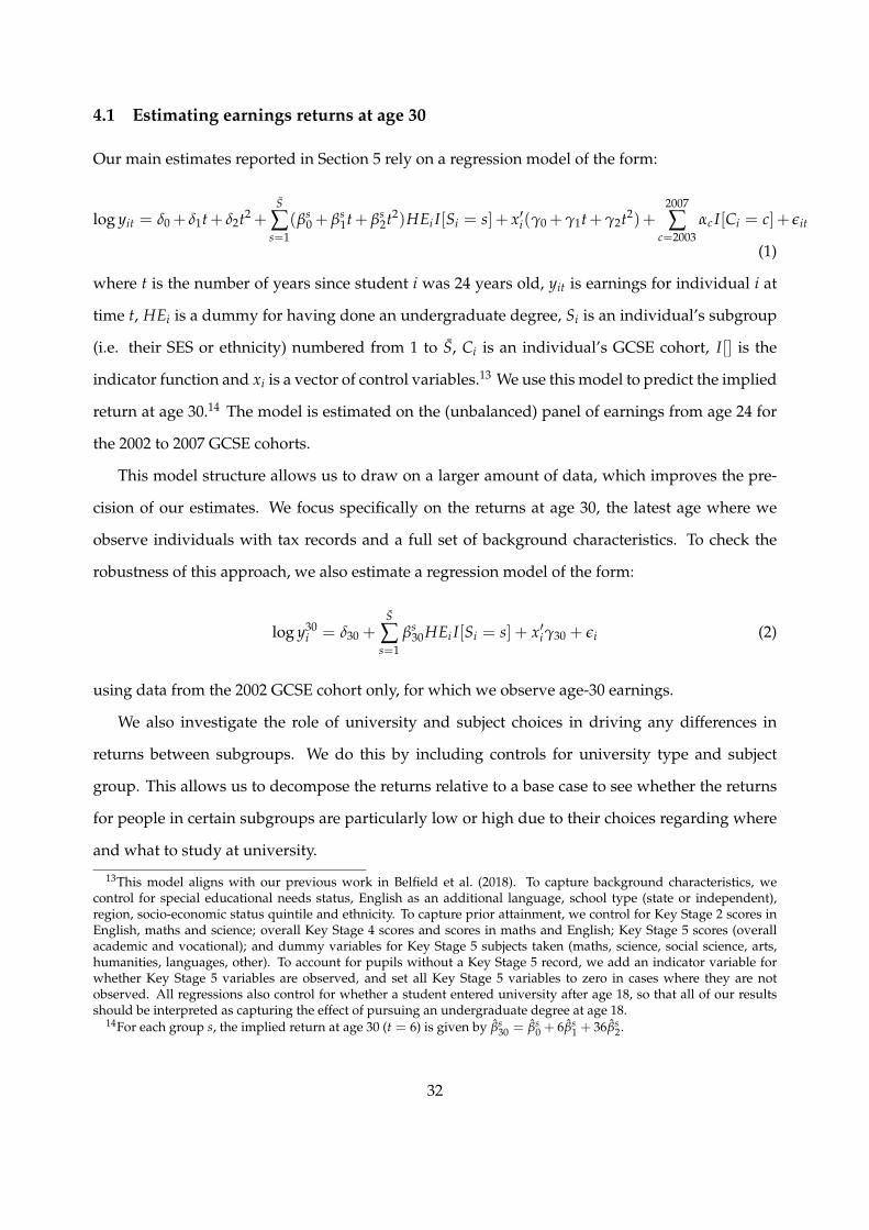
4.1 Estimating earnings returns at age 30
Our main estimates reported in Section 5 rely on a regression model of the form:
log yit = δ0 + δ1t+ δ2t2 +S
∑s=1
(βs0 + βs
1t+ βs2t2)HEi I[Si = s]+ x′i(γ0 +γ1t+γ2t2)+
2007
∑c=2003
αc I[Ci = c]+ εit
(1)
where t is the number of years since student i was 24 years old, yit is earnings for individual i at
time t, HEi is a dummy for having done an undergraduate degree, Si is an individual’s subgroup
(i.e. their SES or ethnicity) numbered from 1 to S, Ci is an individual’s GCSE cohort, I[] is the
indicator function and xi is a vector of control variables.13 We use this model to predict the implied
return at age 30.14 The model is estimated on the (unbalanced) panel of earnings from age 24 for
the 2002 to 2007 GCSE cohorts.
This model structure allows us to draw on a larger amount of data, which improves the pre-
cision of our estimates. We focus specifically on the returns at age 30, the latest age where we
observe individuals with tax records and a full set of background characteristics. To check the
robustness of this approach, we also estimate a regression model of the form:
log y30i = δ30 +
S
∑s=1
βs30HEi I[Si = s] + x′iγ30 + εi (2)
using data from the 2002 GCSE cohort only, for which we observe age-30 earnings.
We also investigate the role of university and subject choices in driving any differences in
returns between subgroups. We do this by including controls for university type and subject
group. This allows us to decompose the returns relative to a base case to see whether the returns
for people in certain subgroups are particularly low or high due to their choices regarding where
and what to study at university.
13This model aligns with our previous work in Belfield et al. (2018). To capture background characteristics, wecontrol for special educational needs status, English as an additional language, school type (state or independent),region, socio-economic status quintile and ethnicity. To capture prior attainment, we control for Key Stage 2 scores inEnglish, maths and science; overall Key Stage 4 scores and scores in maths and English; Key Stage 5 scores (overallacademic and vocational); and dummy variables for Key Stage 5 subjects taken (maths, science, social science, arts,humanities, languages, other). To account for pupils without a Key Stage 5 record, we add an indicator variable forwhether Key Stage 5 variables are observed, and set all Key Stage 5 variables to zero in cases where they are notobserved. All regressions also control for whether a student entered university after age 18, so that all of our resultsshould be interpreted as capturing the effect of pursuing an undergraduate degree at age 18.
14For each group s, the implied return at age 30 (t = 6) is given by βs30 = βs
0 + 6βs1 + 36βs
2.
32

4.2 Simulating lifetime earnings
To simulate earnings for individuals in the 2002 GCSE cohort, we follow Britton et al. (2020) and
estimate a copula model that predicts the percentile rank in the earnings distribution for individ-
uals at any age t, conditional on their position in the distribution in the previous year, t− 1, and
the year before that, t− 2.
For the HE group, we use HMRC data for estimating the copula up until age 40, while for the
non-HE group we can only use HMRC data up to age 30. We therefore use LFS data for ages 40–67
for the HE group and for ages 30–67 for the non-HE group. Where we use LFS data, we have to
use a more stripped-back model where rank next year only depends on rank this year. In general,
we estimate the copula model separately by gender, university group and subject. Where we run
into sample size difficulties, we sometimes pool some of these subgroups.
The advantage of the copula approach is that we can use it to simulate rank at each age inde-
pendently of the actual levels of earnings in the cross-section. We then take cross-sectional earn-
ings distributions at each age from the HMRC data up to age 40 for the HE group and up to age 30
for the non-HE group, and from the LFS otherwise, up to age 67. Cross-sectional distributions are
further split by socio-economic status and ethnicity. We also model employment/unemployment
and re-entry earnings based on the same data sources.
4.3 Estimating lifetime returns
We then use our simulated lifetime earnings profiles to estimate the overall lifetime returns to
higher education. For returns after age 30, we broadly follow the approach of equation (2), but
hold the parameter vector governing the effect of background conditions fixed at its estimated
age-30 value (γ30). In particular, for each age a, we estimate
log yia = δa +S
∑s=1
βsaHEi I[s = S] + εia (3)
where
log yia = log yia − x′iγ30. (4)
33

Once we have our returns estimates at each age a, we can construct the counterfactual earnings
path for each individual.
To calculate the discounted present value of lifetime returns, we remove taxes and student
loan repayments (if appropriate) and add maintenance loans received (if appropriate) from both
the simulated and counterfactual profiles. We then subtract net counterfactual earnings from the
net simulated (or actual) earnings at each age. We sum differences across all ages, applying a
discount factor that discounts returns that occur a long time into the future by more.15
5 Early-career returns
We now present our estimation results. In Section 5.1, we investigate gross earnings returns by
SES and ethnicity at age 30, the latest age at which we observe earnings records and a full set of
conditioning variables. We then turn in Section 5.2 to the importance of subject and university
choices in determining the differences in returns across the different groups. Section 5.3 reports
the implied unexplained differences in earnings between socio-economic and ethnic groups for
both graduates and non-graduates.
5.1 Gross returns at age 30
Table 5 shows the returns estimates for the different SES groups, separately by gender.16 It shows
the sequential addition of control variables in the three columns. We see that the control variables
make a very large difference to the returns estimates. This is almost entirely driven by the prior
attainment controls, which dramatically reduce the returns estimates.
15For this, we use a discount rate of 3.5% for the first 30 years and 3.0% thereafter, based on recommendations fromthe Treasury’s Green Book. For further details, see Britton et al. (2020).
16For a graphical illustration of these results, see Figure A8 in the appendix.
34
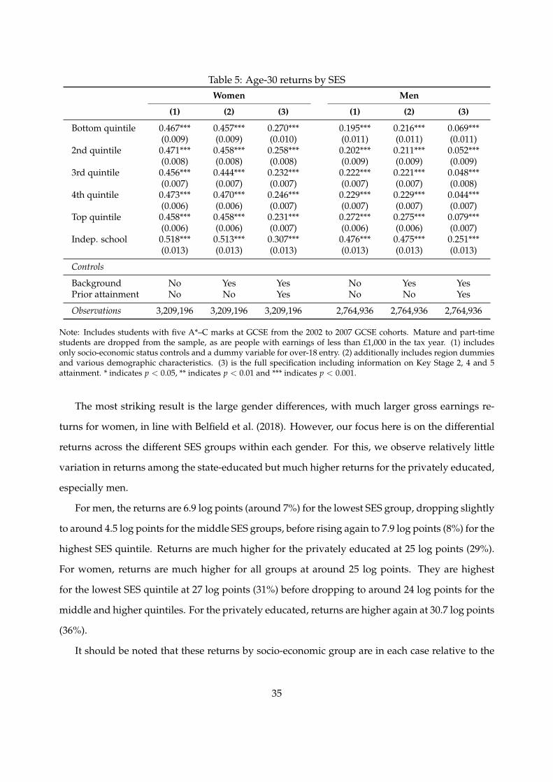
Table 5: Age-30 returns by SESWomen Men
(1) (2) (3) (1) (2) (3)
Bottom quintile 0.467*** 0.457*** 0.270*** 0.195*** 0.216*** 0.069***(0.009) (0.009) (0.010) (0.011) (0.011) (0.011)
2nd quintile 0.471*** 0.458*** 0.258*** 0.202*** 0.211*** 0.052***(0.008) (0.008) (0.008) (0.009) (0.009) (0.009)
3rd quintile 0.456*** 0.444*** 0.232*** 0.222*** 0.221*** 0.048***(0.007) (0.007) (0.007) (0.007) (0.007) (0.008)
4th quintile 0.473*** 0.470*** 0.246*** 0.229*** 0.229*** 0.044***(0.006) (0.006) (0.007) (0.007) (0.007) (0.007)
Top quintile 0.458*** 0.458*** 0.231*** 0.272*** 0.275*** 0.079***(0.006) (0.006) (0.007) (0.006) (0.006) (0.007)
Indep. school 0.518*** 0.513*** 0.307*** 0.476*** 0.475*** 0.251***(0.013) (0.013) (0.013) (0.013) (0.013) (0.013)
Controls
Background No Yes Yes No Yes YesPrior attainment No No Yes No No Yes
Observations 3,209,196 3,209,196 3,209,196 2,764,936 2,764,936 2,764,936
Note: Includes students with five A*–C marks at GCSE from the 2002 to 2007 GCSE cohorts. Mature and part-timestudents are dropped from the sample, as are people with earnings of less than £1,000 in the tax year. (1) includesonly socio-economic status controls and a dummy variable for over-18 entry. (2) additionally includes region dummiesand various demographic characteristics. (3) is the full specification including information on Key Stage 2, 4 and 5attainment. * indicates p < 0.05, ** indicates p < 0.01 and *** indicates p < 0.001.
The most striking result is the large gender differences, with much larger gross earnings re-
turns for women, in line with Belfield et al. (2018). However, our focus here is on the differential
returns across the different SES groups within each gender. For this, we observe relatively little
variation in returns among the state-educated but much higher returns for the privately educated,
especially men.
For men, the returns are 6.9 log points (around 7%) for the lowest SES group, dropping slightly
to around 4.5 log points for the middle SES groups, before rising again to 7.9 log points (8%) for the
highest SES quintile. Returns are much higher for the privately educated at 25 log points (29%).
For women, returns are much higher for all groups at around 25 log points. They are highest
for the lowest SES quintile at 27 log points (31%) before dropping to around 24 log points for the
middle and higher quintiles. For the privately educated, returns are higher again at 30.7 log points
(36%).
It should be noted that these returns by socio-economic group are in each case relative to the
35

non-HE baseline for that group. So, for example, the estimated return for people from the bottom
socio-economic group takes into account that non-graduates from that group tend to have lower
incomes than those from wealthier backgrounds, even conditional on their school attainment and
other background conditions. As a result, unexplained differences in non-graduate earnings be-
tween groups can be as much of a driver of differences in returns as are differences in graduate
earnings.17
The relatively high returns for students from the bottom SES quintile are consistent with Card’s
(2001) observation that instrumental variables estimates of the return to education are typically
larger than OLS estimates. He suggests an explanation based on the marginal cost of education: if
the marginal cost of education is higher for marginal students, we would expect to observe high
returns for those who do decide to go. By the same mechanism, we might estimate high returns for
the bottom SES quintile, because among that group, only those with the highest expected returns
from attending university actually decide to go.
A striking result is the high returns for independent school students, especially for men. This
is partly attributable to very high earnings for some university graduates who went to private
school. Perhaps more surprisingly, it is also partly due to the relatively modest earnings (given
their high school attainment) of independent school students who do not go on to university.
For men in particular, as shown in Figure 4, median non-HE earnings at age 30 are lower for the
privately-educated than for all except the poorest state school groups, despite much higher GCSE
attainment.
A variety of explanations could account for this finding. First, those who attend independent
schools may delay labour market entry, leading to lower pay at the same age due to lower labour
market experience. Second, those who went to independent school may choose to work fewer
hours or in less lucrative occupations as a result of higher family wealth. Third, as a larger share
of independent school students go to university, non-graduates may be more negatively selected
on unobservables such as health, leading to bias. Fourth, if independent schools prepare students
better for standardised tests, these students’ prior attainment scores may overstate their true abil-
ity, which would also lead to biased estimates. Fifth, our data do not capture the dividend income
17Unexplained conditional differences in earnings between socio-economic groups, as estimated in the same regres-sion model, are shown in Table A3 in the appendix.
36

of business owners running limited companies, which might be disproportionately important for
this demographic.
Table 6: Age-30 returns by ethnicityWomen Men
(1) (2) (3) (1) (2) (3)
White British 0.487*** 0.459*** 0.244*** 0.253*** 0.231*** 0.058***(0.004) (0.004) (0.004) (0.004) (0.004) (0.005)
White Other 0.473*** 0.439*** 0.224*** 0.297*** 0.270*** 0.109***(0.021) (0.021) (0.021) (0.022) (0.022) (0.022)
Black Caribbean 0.285*** 0.240*** 0.090* 0.206*** 0.191*** 0.065(0.036) (0.036) (0.035) (0.041) (0.040) (0.040)
Black African 0.340*** 0.306*** 0.180*** 0.284*** 0.280*** 0.140*(0.053) (0.053) (0.052) (0.056) (0.056) (0.055)
Black Other 0.402*** 0.364*** 0.208*** 0.212*** 0.187*** 0.035(0.050) (0.050) (0.049) (0.054) (0.054) (0.053)
Indian 0.439*** 0.405*** 0.240*** 0.331*** 0.303*** 0.151***(0.029) (0.028) (0.028) (0.028) (0.028) (0.028)
Pakistani 0.534*** 0.495*** 0.333*** 0.464*** 0.444*** 0.306***(0.029) (0.029) (0.029) (0.033) (0.033) (0.033)
Bangladeshi 0.461*** 0.436*** 0.266*** 0.297*** 0.274*** 0.132**(0.041) (0.040) (0.040) (0.046) (0.046) (0.045)
Chinese 0.257*** 0.255*** 0.137 0.325*** 0.321*** 0.197**(0.073) (0.073) (0.071) (0.068) (0.067) (0.066)
Other 0.478*** 0.443*** 0.225*** 0.278*** 0.264*** 0.082***(0.014) (0.014) (0.014) (0.014) (0.014) (0.014)
Controls
Background No Yes Yes No Yes YesPrior attainment No No Yes No No Yes
Observations 2,830,229 2,830,229 2,830,229 2,402,885 2,402,885 2,402,885
Note: Includes state-educated students with five A*–C marks at GCSE from the 2002 to 2007 GCSE cohorts. Matureand part-time students are dropped from the sample, as are people with earnings of less than £1,000 in the tax year.(1) includes only ethnicity controls and a dummy variable for over-18 entry. (2) additionally includes region dummiesand various demographic characteristics. (3) is the full specification including information on Key Stage 2, 4 and 5attainment. * indicates p < 0.05, ** indicates p < 0.01 and *** indicates p < 0.001.
Table 6 then shows returns estimates by ethnicity.18 Again, we see the raw differences heavily
reduced by the inclusion of control variables, and again it is the prior attainment controls that
make by far the most difference to our estimates, despite the large regional variation in ethnicity
shares that we saw in Section 3.3. It is notable that many of these groups are quite small and
therefore the estimates are relatively imprecise, even with the panel structure that we use to boost
18For a graphical illustration of these results, see Figure A9 in the appendix. For unexplained conditional differencesin earnings by ethnicity from the same regression, see Table A4 in the appendix.
37
our sample sizes by incorporating multiple cohorts.
For women, we observe large and significantly positive returns for all groups except Chinese
students.19 South Asian students do particularly well, with Indian (24.0 log points or 27%), Pak-
istani (33.3 log points, 40%) and Bangladeshi (26.6 log points, 30%) students all achieving large
returns. Estimated returns for Black women are somewhat lower than for White women. Returns
for Black Caribbean women are particularly low at 9.0 log points (9%).
For men, we again observe on average much lower returns, but notably all point estimates
are positive. The largest estimates by some distance are for Pakistani students at 30.6 log points
(36%), while returns are also high for Indian students (15.1 log points or 16%) and for Chinese
students (19.7 log points or 22%), but the latter are imprecisely estimated. Returns for White
British students are close to the overall age-29 estimates from Belfield et al. (2018) and are precisely
estimated, as they are by far the largest group.
5.2 Importance of institution and subject choices in age-30 returns
Importantly, the above estimates do not control for institution and subject choices. Yet these could
be very important drivers of returns – we know from Belfield et al. (2018) that different institutions
and subjects can dramatically affect earnings prospects, and from Section 3 that the distributions
of subjects and university types are very different across our different subgroups. For example,
the privately educated are much more likely to attend the elite Russell Group institutions than any
of the other SES groups, while there are also very different patterns in subject choices by SES.
In Tables 7 and 8, we show the impact of controlling for institution and subject choices on our
returns estimates, separately by gender.20 We can only control for subject and institution within
the set of people who go to university, as there is no such thing as an institution or subject for
those who do not go to university. We therefore show how the effect sizes change relative to a base
case. In each case, we first show the equivalent returns estimates to before, but now relative to the
base case. We then add in subject controls and finally institution controls.
Table 7 shows our estimates by SES, with the highest SES quintile among state school students
(the largest group) as the reference group. In the first column, we see that returns for the bottom
19Returns for Chinese students are imprecisely estimated for both women and men due to the very small share ofChinese students in our sample who do not go on to higher education.
20We also show these estimates graphically in Figures A10 and A11 in the appendix.
38

quintile are 4.0 log points higher for women and almost identical for men, reproducing the results
from above. In the second column, we add subject controls and see that the relative returns mostly
go down. This implies that the highest state school SES group chooses lower-return subjects rel-
ative to the other groups; if all groups made the same subject choices as the highest state school
SES group, their returns would be lower. It is especially notable that the relative returns estimates
decrease for the lowest SES groups, suggesting that their relatively high returns are partly driven
by their subject choices. This is likely driven by the high share of such students selecting relatively
high-returning business, law and computing degrees.
Table 7: Impact of subject and institution on relative returns by SESWomen Men
(1) (2) (3) (1) (2) (3)
Bottom quintile 0.040*** 0.033** 0.045*** -0.010 -0.021 -0.002(0.011) (0.011) (0.011) (0.012) (0.012) (0.012)
2nd quintile 0.027** 0.024* 0.035*** -0.027* -0.029** -0.014(0.010) (0.009) (0.009) (0.010) (0.010) (0.010)
3rd quintile 0.001 -0.001 0.007 -0.031*** -0.027** -0.018*(0.009) (0.009) (0.009) (0.009) (0.009) (0.009)
4th quintile 0.016 0.016 0.022** -0.034*** -0.031*** -0.024**(0.008) (0.008) (0.008) (0.009) (0.009) (0.009)
Indep. school 0.076*** 0.066*** 0.050*** 0.172*** 0.166*** 0.136***(0.014) (0.014) (0.014) (0.014) (0.014) (0.013)
Controls
Subject No Yes Yes No Yes YesUniversity No No Yes No No Yes
Observations 3,209,196 3,209,196 3,209,196 2,764,936 2,764,936 2,764,936
Note: The top quintile of state-educated students is the omitted category. Includes students with five A*–C marks atGCSE from the 2002 to 2007 GCSE cohorts. Mature and part-time students are dropped from the sample, as are peoplewith earnings of less than £1,000 in the tax year. (1) restates the main returns results by socio-economic status relativeto the omitted category. (2) includes a full set of controls for subject studied. (3) also controls for university attended. *indicates p < 0.05, ** indicates p < 0.01 and *** indicates p < 0.001.
When we include institution controls, however, we see that returns estimates generally go
up again, suggesting that the highest SES quintile, on average, chooses institutions with higher
returns. For the state-educated, this takes the estimates back above the overall relative estimates,
meaning that the adverse earnings effects of institution choices outweigh the positive effects of
subject choices in these cases.
For the privately educated, returns again go down, suggesting that both their subject and uni-
39

versity choices benefit their earnings relative to the highest SES base case. This is perhaps un-
surprising given the very high share of privately educated students at top universities and the
dominance of these students in the higher-earning subjects, although it is important to note that
the results here show the effects of subject and institution choices conditional on prior attainment.
Table 8: Impact of subject and institution on relative returns by ethnicityWomen Men
(1) (2) (3) (1) (2) (3)
White Other -0.021 -0.023 -0.029 0.051* 0.046* 0.034(0.021) (0.021) (0.021) (0.022) (0.022) (0.022)
Black Caribbean -0.154*** -0.166*** -0.168*** 0.007 -0.005 -0.001(0.035) (0.035) (0.035) (0.040) (0.040) (0.040)
Black African -0.064 -0.111* -0.120* 0.082 0.032 0.023(0.052) (0.051) (0.051) (0.055) (0.055) (0.055)
Black Other -0.037 -0.053 -0.052 -0.024 -0.039 -0.041(0.049) (0.048) (0.048) (0.053) (0.053) (0.053)
Indian -0.004 -0.063* -0.078** 0.093*** 0.022 -0.001(0.028) (0.028) (0.028) (0.028) (0.028) (0.028)
Pakistani 0.089** 0.024 0.014 0.248*** 0.173*** 0.178***(0.029) (0.028) (0.028) (0.033) (0.032) (0.032)
Bangladeshi 0.022 -0.015 -0.018 0.074 0.003 0.004(0.040) (0.039) (0.039) (0.045) (0.045) (0.045)
Chinese -0.108 -0.149* -0.168* 0.138* 0.088 0.063(0.072) (0.071) (0.071) (0.066) (0.066) (0.065)
Other -0.019 -0.028* -0.033* 0.024 0.009 0.002(0.014) (0.014) (0.013) (0.014) (0.014) (0.014)
Controls
Subject No Yes Yes No Yes YesUniversity No No Yes No No Yes
Observations 2,830,229 2,830,229 2,830,229 2,402,885 2,402,885 2,402,885
Note: White British is the omitted category. Includes state-educated students with five A*–C marks at GCSE from the2002 to 2007 GCSE cohorts. Mature and part-time students are dropped from the sample, as are people with earningsof less than £1,000 in the tax year. (1) restates the main returns results by ethnicity relative to the omitted category.(2) includes a full set of controls for subject studied. (3) also controls for university attended. * indicates p < 0.05, **indicates p < 0.01 and *** indicates p < 0.001.
Table 8 shows the equivalent estimates by ethnicity, all relative to the White British case. We
now see that all estimates drop once we include the subject controls. This suggests that, on av-
erage, White British students are choosing subjects with lower earnings potential than ethnic mi-
nority groups. The biggest drops in returns are for Asian and Black African students, reflecting
the high propensity of these students to choose subjects with high earnings potential such as busi-
ness and pharmacology. On the other hand, we see only negligible changes to the relative returns
40

estimates for Black Caribbean and Black Other students, suggesting that they choose subjects that
have very similar earnings potential to those chosen by White British students.
Finally, when we include the institution controls in column 3, we generally see only quite small
changes compared with column 2. For Indian and Chinese students, the estimates drop again,
suggesting they tend to choose institutions with higher earnings potential, but the differences
are very small. Notably, after adding in subject and institution controls, the unexplained returns
difference from White British students is statistically insignificant for most groups.
5.3 Unexplained differences in earnings
The relative return for each group is directly related to the unexplained differences in earnings
between groups: the relative return to HE for each group is the difference between graduates and
non-graduates of a given group in the unexplained difference in earnings between that group and
a reference group. While the focus of this report is on differences in returns, this section shows
unexplained differences in earnings between groups, for both graduates and non-graduates, to
put these differences in returns in context.21 A key finding is that unexplained differences in
earnings are mostly smaller for graduates than for non-graduates, implying that differences in
the returns to higher education ‘even out’ some of the unexplained earnings differences between
non-graduates.
Figure 15 shows the unexplained gaps in earnings between SES groups after controlling for the
full set of explanatory variables as in column 3 of Table 7. Differences for graduates are relative to
graduates from the top SES quintile of the state-educated, and differences for non-graduates are
relative to non-graduates from the top SES quintile of the state-educated. Whiskers indicate the
95% confidence interval.22
21As for returns, we only look at differences between groups within each gender, as all of our analysis is done com-pletely seperately for men and women. For evidence on how much of the difference in earnings between graduate menand women can be explained by observable differences such as subject choices, see Figure A3 in the appendix.
22 Unexplained gaps for independent school students are not reported, as they are not meaningful. The reason is thatschool records from independent schools contain a smaller set of background variables, so any estimated differencebetween state and independent school students will be biased by the effect of the missing background variables.
41

Figure 15: Unexplained earnings gaps between SES groups: HE and non-HE
-13%
-11%
-10%
-8%
-6%
-4%
-2%
0%
-14
-12
-10
-8-6
-4-2
0R
esid
ual d
iffer
ence
in e
arni
ngs
(in lo
g po
ints
)
Bottom
Quin
tile
2nd Q
uintile
3rd Q
uintile
4th Q
uintile
HE non-HE 95% CI
Women
-13%
-11%
-10%
-8%
-6%
-4%
-2%
0%
-14
-12
-10
-8-6
-4-2
0R
esid
ual d
iffer
ence
in e
arni
ngs
(in lo
g po
ints
)
Bottom
Quin
tile
2nd Q
uintile
3rd Q
uintile
4th Q
uintile
HE non-HE 95% CI
Men
Note: Unexplained gaps in earnings between SES groups after controlling for the full set of explanatory variables as incolumn 3 of Table 7. The top quintile of state-educated students is the omitted category. The vertical distance betweenHE and non-HE markers is the relative return reported in column 3 of Table 7. Includes people with five A*–C marksat GCSE. Mature and part-time students are dropped from the sample, as are people with earnings of less than £1,000in the tax year. Unexplained gaps for independent school students are not reported, as they are not meaningful (see fn.22).
After accounting for our full set of controls, both female and male graduates and non-graduates
from nearly all other SES groups earn significantly less than the top SES quintile of the state-
educated.23 There is a clear gradient with socio-economic background for both graduates and non-
graduates, with those from lower socio-economic groups earning less after controlling for our full
set of control variables. For women, the unexplained earnings gaps between different groups are
smaller for graduates than for non-graduates. This suggests that conditional on prior attainment
and other background characteristics, university attenuates differences between women from dif-
23The only exception is men from the second-highest SES group among the state-educated, who earn insignificantlyless.
42

ferent socio-economic backgrounds.
Figure 16: Unexplained earnings gaps between ethnic groups: HE and non-HE
-33%
-26%
-18%
-10%
0%11
%22
%35
%49
%
-40
-30
-20
-10
010
2030
40R
esid
ual d
iffer
ence
in e
arni
ngs
(in lo
g po
ints
)
Whit
e Othe
r
Black C
aribb
ean
Black A
frican
Black O
ther
Indian
Pakist
ani
Bangla
desh
i
Chines
eOthe
r
HE non-HE 95% CI
Women
-33%
-26%
-18%
-10%
0%11
%22
%35
%49
%
-40
-30
-20
-10
010
2030
40R
esid
ual d
iffer
ence
in e
arni
ngs
(in lo
g po
ints
)
Whit
e Othe
r
Black C
aribb
ean
Black A
frican
Black O
ther
Indian
Pakist
ani
Bangla
desh
i
Chines
eOthe
r
HE non-HE 95% CI
Men
Note: Unexplained gaps in earnings between ethnic groups after controlling for the full set of explanatory variables asin column 3 of Table 8. White British is the omitted category. The vertical distance between HE and non-HE markersis the relative return reported in column 3 of Table 8. Includes state-educated students with five A*–C marks at GCSE.Mature and part-time students are dropped from the sample, as are people with earnings of less than £1,000 in the taxyear.
Figure 16 is the equivalent figure for different ethnic groups. The omitted category is White
British, so differences for graduates are relative to White British graduates, and differences for
non-graduates are relative to White British non-graduates. Unexplained differences in earnings
between ethnic groups are smaller for graduates than for non-graduates for both women and men.
For women, this is because Black, Indian and Chinese non-graduates have substantially higher con-
ditional earnings than White British women, which is not the case for graduate women (although
note that the confidence intervals for non-HE women from these ethnic groups are wide). For
men, this is largely driven by the results for Pakistani men: for Pakistani non-graduates, condi-
43

tional earnings are nearly 40 log points lower than those of White British non-graduates, whereas
the same figure for graduates is less than 20 log points. This suggests that going to university can
help level the playing field between people from different ethnic groups to some extent.
Nonetheless, the results presented in Figure 16 also point to significant unexplained earnings
differences between graduates from different ethnic groups. Results for men – which are easier to
interpret as a large majority of men work full time – suggest that not only non-graduates but also
graduates from all ethnic groups except White Other have significantly lower earnings than White
British men after controlling for a large array of potential confounding factors. This may reflect
the effects of labour market discrimination.
6 Lifetime earnings
We now consider returns to higher education at different ages and across the lifetime. As these
returns are based on long-run earnings projections, they are subject to a much higher degree of
uncertainty than the estimates in Section 5.24 Before discussing the returns estimates, we start by
reporting some of the results from our lifetime simulation exercise. We then move on to show
our estimates of returns at ages 30, 40 and 50 drawing on these simulations. Finally, we show our
estimates of the discounted net present value of attending higher education.25
24It should also be noted that this section is aligned with Britton et al. (2020) rather than with Belfield et al. (2018) interms of methodology and sample selection, which can explain minor discrepancies between the estimates.
25We exclude ‘Black Other’ and ‘Chinese’ throughout this section. The reason is that these groups are so small thatno reliable statements about lifetime earnings and returns can be made.
44

Figure 17: Predicted net lifetime earnings by SES
10th perc.25th perc.
50th perc.
75th perc.90th perc.
mean
Key:
050
010
0015
00
Net
Dis
coun
ted
Life
time
Ear
ning
s (in
k£)
Bo
ttom
Qui
ntile
2nd
Qui
ntile
3rd
Qui
ntile
4th
Qui
ntile
Top
Qui
ntile
Inde
p. S
choo
l
HE Non-HE
Women
050
010
0015
00
Net
Dis
coun
ted
Life
time
Ear
ning
s (in
k£)
Bo
ttom
Qui
ntile
2nd
Qui
ntile
3rd
Qui
ntile
4th
Qui
ntile
Top
Qui
ntile
Inde
p. S
choo
l
HE Non-HE
Men
Note: Predicted real lifetime earnings after taxes and student loan repayments, discounted using Green Book discount-ing, based on predictions for the 2002 GCSE cohort. Includes students with five A*–C marks at GCSE and a Key Stage5 record. Mature and part-time students are dropped from the sample.
6.1 Lifetime earnings simulations
Figure 17 documents the distribution of the projected net discounted present value of lifetime
earnings for each of the SES groups, by gender and HE status. It plots not only the mean but also
the 10th, 25th, 50th, 75th and 90th percentiles from the distribution.
We observe a clear SES gradient in the means amongst the HE group, for both men and women.
For women, the mean net discounted present value of lifetime earnings increases from £540,000
for the lowest SES quintile to around £570,000 for the highest SES quintile and around £590,000
for those from independent schools. In terms of (non-discounted) average net annual earnings
between ages 18 and 67, this roughly corresponds to £24,000 for the bottom quintile, £25,000 for
45

the top quintile and £26,000 for those who went to independent schools. For men, the gradient
is steeper, with an upward tick for those from independent schools. Interestingly, there does not
appear to be much of a social gradient in the lower percentiles of the distribution, while there
is a very strong gradient amongst the higher percentiles. Most notably, the 90th percentile of net
discounted present value of lifetime earnings for men from independent schools is well above £1.5
million, corresponding to life-cycle average non-discounted net annual earnings of £77,000.26
Interestingly, the SES gradient is less clear amongst the non-HE group. In particular, mean
net discounted present values of lifetime earnings are lower amongst the non-HE group from
independent schools than for those in the highest SES quintile, for both men and women.
Figure 18 then plots the equivalent figure by ethnicity group, although for this we only show
the mean rather than the distribution due to the smaller sample size. It is sorted on the mean of net
discounted present value lifetime earnings of the HE group. Indian and White Other are at the top
end for both men and women and Pakistani students at the bottom end. For men, the discounted
present value of net lifetime earnings is around £800,000 for Indian HE students (annual average
non-discounted earnings of £38,000), while for Pakistani students it is around £700,000 (annual
average non-discounted net earnings of £32,000). For women, the estimates range from just over
£600,000 (annual average £27,000) for Indian HE students to around £530,000 for Pakistani stu-
dents (annual average £24,000).
There is also quite a lot of variation in lifetime earnings for the non-HE groups. For women
these typically range between £300,000 and £400,000 (average net annual earnings of £14,000 to
£17,000), while for men they are typically between £500,000 and £550,000 (average net annual
earnings of £21,000 to £25,000). The exception to this is Pakistani men, for whom non-HE lifetime
earnings are only just above £400,000. Indeed, the gaps between HE and non-HE for Pakistani
students is notably large for both men and women.
26This may reflect an effect identified by Zimmerman (2019) using data from Chile: men from independent schoolsat elite universities appear to form ties with classmates from similar backgrounds, which helps these students achievehigher managerial positions.
46

Figure 18: Predicted net lifetime earnings by ethnicity30
040
050
060
070
080
0
Net
Dis
coun
ted
Life
time
Ear
ning
s (in
k£)
Pa
kista
niBa
ngla
desh
iBl
ack
Carib
bean
Whi
te B
ritish
Oth
erW
hite
Oth
erBl
ack
Afric
anIn
dian
HE Non-HE
Women
300
400
500
600
700
800
Net
Dis
coun
ted
Life
time
Ear
ning
s (in
k£)
Bl
ack
Carib
bean
Pakis
tani
Blac
k Af
rican
Whi
te B
ritish
Bang
lade
shi
Oth
erW
hite
Oth
erIn
dian
HE Non-HE
Men
Note: Mean predicted real lifetime earnings after taxes and student loan repayments, discounted using Green Bookdiscounting, based on predictions for the 2002 GCSE cohort. Includes state-educated students with five A*–C marks atGCSE and a Key Stage 5 record. Mature and part-time students are dropped from the sample.
6.2 Gross returns at older ages
We now draw on the lifetime simulations to estimate gross earnings returns at later points in the
life cycle than we estimated in the previous section. Figures 19 and 20 show the returns at ages 30,
40 and 50 by SES and ethnicity, respectively, done separately by gender.27
27The sample restrictions and model specification in this section fully align with Britton et al. (2020) to guarantee thecomparability of lifetime returns estimates. As a result, the age-30 returns presented in these plots do not preciselymatch the results presented in the previous section.
47

Figure 19: Gross returns at older ages by SES
Bottom Quintile
2nd Quintile
3rd Quintile
4th Quintile
Top Quintile
Indep. School
0% 11% 22% 35% 49% 65%
Return (in %)
0 10 20 30 40 50
Return (Log Points)
Age 30 Age 40 Age 50
Women
0% 11% 22% 35% 49% 65%
Return (in %)
0 10 20 30 40 50
Return (Log Points)
Age 30 Age 40 Age 50
Men
Note: Includes students with five A*–C marks at GCSE and a Key Stage 5 record from the 2002 GCSE cohort only.Mature and part-time students are dropped from the sample. The effect of background conditions is held constant atage-30 levels, as explained in Section 4.
From Figure 19, we see that returns to higher education grow for all groups after age 30. For
both men and women, we observe large earnings growth between ages 30 and 40, although the
growth is more substantial for men, considerably reducing the differences in average returns be-
tween men and women. After age 40, returns level off for men, although they continue to grow
for the lower SES groups. For women, on the other hand, they shrink back towards the age-30 es-
timates (although less so for the lower SES groups), perhaps reflecting increases in working hours
amongst non-HE women at these ages. Interestingly, for both men and women, growth in returns
after age 30 is largest for the bottom SES quintile; later-life returns for this group are very large at
over 50% for both genders.
48

Figure 20: Gross returns at older ages by ethnicity
White British
White Other
Black Caribbean
Black African
Indian
Pakistani
Bangladeshi
Other
-18% 0% 22% 49% 82% 123%
Return (in %)
-20 0 20 40 60 80
Return (Log Points)
Age 30 Age 40 Age 50
Women
-18% 0% 22% 49% 82% 123%
Return (in %)
-20 0 20 40 60 80
Return (Log Points)
Age 30 Age 40 Age 50
Men
Note: Includes state-educated students with five A*–C marks at GCSE and a Key Stage 5 record from the 2002 GCSEcohort only. Mature and part-time students are dropped from the sample. The effect of background conditions is heldconstant at age-30 levels, as explained in Section 4.
Figure 20 then shows the equivalent estimates by ethnicity. Again, we see large growth in
returns after age 30 for both men and women (noting that the scale is slightly different from that
on Figure 19). Again we see returns falling back after age 40 for women in most cases, and a
levelling-off effect for men. The most notable growth in returns is for Pakistani and Bangladeshi
students, who are projected to see very substantial increases after age 30.
6.3 Lifetime returns
We now consider how these differences in gross returns at specific points in time translate into
lifetime returns. Our headline estimates are in discounted net present value terms, which means
they account for any change in earnings associated with attending, any change in taxes and any
49

net loss (or gain) from student loans.28 They also discount returns that occur in the future at the
Treasury Green Book discount rate of 3.5% in the first 30 years and 3% thereafter. The easiest
way to interpret the estimates is that they roughly capture what going to university is worth, on
average, to individuals at the point when they make the decision over whether to go or not.
Figure 21: Predicted net lifetime returns by SES
10th perc.25th perc.
50th perc.
75th perc.90th perc.
mean
Key:
-200
020
040
060
0
Net
Dis
coun
ted
Life
time
Ret
urns
(in
k£)
Bo
ttom
Qui
ntile
2nd
Qui
ntile
3rd
Qui
ntile
4th
Qui
ntile
Top
Qui
ntile
Inde
p. S
choo
l
Women
-200
020
040
060
0
Net
Dis
coun
ted
Life
time
Ret
urns
(in
k£)
Bo
ttom
Qui
ntile
2nd
Qui
ntile
3rd
Qui
ntile
4th
Qui
ntile
Top
Qui
ntile
Inde
p. S
choo
l
Men
Note: Returns are net of taxes and student loan repayments and discounted using Green Book discounting. Includesstudents with five A*–C marks at GCSE and a Key Stage 5 record from the 2002 GCSE cohort only. Mature and part-time students are dropped from the sample.
Figure 21 shows the estimates by SES group. We observe a U shape in the relationship between
SES and lifetime returns. For women, the return for the bottom quintile group is around £140,000.
This drops to around £100,000 for the second to fourth quintiles and drops again to around £70,000
for the top (state) quintile. It jumps back up to around £110,000 for women from independent
schools.28Individuals gain from student loans if they borrow more in maintenance support than the discounted present value
of what they repay in income-contingent loan repayments.
50

For men, the returns are similar to the estimates for women for the bottom four SES quintiles.
However, they are higher for the highest SES quintile, at around £110,000, while for the privately
educated the returns are much higher at around £250,000. These estimates are directly comparable
to the overall average returns estimated in Britton et al. (2020) of £130,000 for men and £100,000
for women.
Figure 22: Share with positive lifetime returns by SES
020
4060
8010
0
Sha
re w
ith P
ositi
ve R
etur
ns (i
n %
)
Botto
m Q
uint
ile2n
d Q
uint
ile3r
d Q
uint
ile4t
h Q
uint
ileTo
p Q
uint
ileIn
dep.
Sch
ool
Women
020
4060
8010
0
Sha
re w
ith P
ositi
ve R
etur
ns (i
n %
)
Botto
m Q
uint
ile2n
d Q
uint
ile3r
d Q
uint
ile4t
h Q
uint
ileTo
p Q
uint
ileIn
dep.
Sch
ool
Men
Note: Returns are net of taxes and student loan repayments and discounted using Green Book discounting. Includesstudents with five A*–C marks at GCSE and a Key Stage 5 record from the 2002 GCSE cohort only. Mature and part-time students are dropped from the sample.
The box plots behind the mean estimates give a sense of the distribution of returns. For women
we see a range of somewhat more than £200,000 between the 10th and 90th percentile returns
estimates, while for men it is typically larger, at more than £300,000. The range is particularly
big for privately educated men, with the difference between the 90th and 10th percentiles being
around £600,000. A quarter of men in this group benefit from higher education by more than
51

£300,000.
We see from the box plots that the lower tails overlap with zero in several cases. This means
that in these groups, there are at least 10% of people for whom the financial benefits of attending
higher education are outweighed by the costs. Figure 22 shows the precise estimated shares with
positive net lifetime returns within each SES group. We see that for women, the share with positive
returns decreases with SES quintile before picking up again for the privately educated, mirroring
the overall returns results. Notably, around 95% of those in the bottom SES quintile who go to
university are projected to benefit financially from doing so, suggesting higher education is a very
good option for women in this group. This share dips to around three-quarters of those from the
top SES quintile who go to university.
Figure 23: Predicted net lifetime returns by ethnicity
050
100
150
200
250
Net
Dis
coun
ted
Life
time
Ret
urns
(in
k£)
Bl
ack
Carib
bean
Whi
te B
ritish
Whi
te O
ther
Oth
erIn
dian
Bang
lade
shi
Pakis
tani
Blac
k Af
rican
Women0
5010
015
020
025
0
Net
Dis
coun
ted
Life
time
Ret
urns
(in
k£)
Bl
ack
Afric
anBl
ack
Carib
bean
Whi
te B
ritish
Whi
te O
ther
Oth
erBa
ngla
desh
iIn
dian
Pakis
tani
Men
Note: Returns are net of taxes and student loan repayments and discounted using Green Book discounting. Includesstate-educated students with five A*–C marks at GCSE and a Key Stage 5 record from the 2002 GCSE cohort only.Mature and part-time students are dropped from the sample.
52

For men, the shares of those attending who gain financially from higher education are uni-
formly lower than for women. Again, we see a drop in the positive shares when we move up
through the SES quintiles, from around 80% of those in the bottom quintile to around two-thirds
of those in the fourth quintile. The share picks up again for the highest SES quintile before increas-
ing to nearly 90% for the privately educated.
Figure 23 then shows the lifetime returns by ethnicity. As before, we only show means and
exclude both Black Other and Chinese students from the figure due to insufficient data. Notably,
the returns for all (other) ethnicity groups are positive. In general, the returns are very high for
South Asian students. For men, Pakistani students have the highest average lifetime returns of
around £220,000, almost double the overall average. For women, Black African students have the
highest average lifetime returns, at around £175,000; this is in stark contrast to Black African men,
for whom we estimate the lowest average lifetime returns at just above £50,000.29
We do not show the distribution plots by ethnicity as we did by SES, partly because the smaller
sample sizes make the distributional estimates much less precise. However, we again give a sense
of the distribution in Figure 24, which shows the estimated shares with positive returns by eth-
nicity. We see that for the ethnicity groups with the highest lifetime returns, almost all university
students are set to benefit financially from attending. For women, the positive shares drop to
around 80% for Black Caribbean, White British, White Other and Other students, while for men
the positive shares fall further, to around two-thirds for Black Caribbean, Black African, White
British and White Other students.29However, it should be noted that Black African students only make up around 1% of all secondary school students,
so these returns are relatively imprecisely estimated.
53

Figure 24: Share with positive lifetime returns by ethnicity0
2040
6080
100
Sha
re w
ith P
ositi
ve R
etur
ns (i
n %
)
Blac
k Ca
ribbe
anW
hite
Oth
erO
ther
Whi
te B
ritish
Indi
anBa
ngla
desh
iBl
ack
Afric
anPa
kista
ni
Women
020
4060
8010
0
Sha
re w
ith P
ositi
ve R
etur
ns (i
n %
)
Blac
k Af
rican
Whi
te B
ritish
Blac
k Ca
ribbe
anW
hite
Oth
erO
ther
Indi
anBa
ngla
desh
iPa
kista
ni
Men
Note: Returns are net of taxes and student loan repayments and discounted using Green Book discounting. Includesstate-educated students with five A*–C marks at GCSE and a Key Stage 5 record from the 2002 GCSE cohort only.Mature and part-time students are dropped from the sample.
7 Conclusion
Our analysis shows that over the whole life cycle, university pays off on average for men and
women from all socio-economic and ethnic groups. Within all groups, more than two-thirds of
university students benefit financially from their degrees. However, there are substantial differ-
ences in average returns between groups.
Returns vary relatively little by socio-economic status, with only those who went to inde-
pendent schools – especially men – getting substantially higher returns from their degrees. Net
lifetime returns are also high for those from the lowest socio-economic backgrounds, especially
for women. At the other end of the spectrum, returns for state-educated men and women near the
54

top of the socio-economic status distribution are relatively modest.
Returns are mostly lower for Black students than for White students, and higher for South
Asian students. In particular, Pakistani graduates achieve very high returns, despite having the
lowest earnings at age 30. Black African women are a possible exception to the rule: we estimate
that they will on average achieve around twice the average net lifetime return of White women,
although this estimate is subject to a large amount of uncertainty.
These differences are partly driven by university and subject choices. There is a clear socio-
economic gradient in university choices, with privately educated students and students from more
advantaged socio-economic backgrounds studying at higher-return institutions. In explaining
differences between ethnic groups, subject choice plays a larger role: ethnic Asian students tend
to choose higher-return subjects than their Black and White peers.
Remaining differences in estimated returns between groups stem from differences between
graduates and non-graduates of different groups that are not explained by their institution and
subject choices, prior attainment or other observable background conditions. These will include
the access to social networks, rates of part-time work, unobserved non-cognitive skills, and the ef-
fects of labour market discrimination. For instance, elite social networks are likely to be important
in explaining the exceptional returns of some men who went to private schools. Differential rates
of part-time work by socio-economic status may be an important factor behind the high estimated
returns of women from poorer families.
Notably, unexplained differences in estimated returns between groups are, to some extent,
the mirror image of unexplained differences in non-graduate earnings conditional on prior at-
tainment and other background conditions. This suggests that, among students from different
socio-economic or ethnic groups but with the same prior attainment and other background char-
acteristics, university education can help level the playing field in the labour market. However,
substantial unexplained differences remain even for graduates. In particular, graduate men from
all ethnic minority groups have lower earnings than male White British graduates even after con-
trolling for prior attainment and a host of other background characteristics.
55

Bibliography
Altonji, Joseph G, Erica Blom, and Costas Meghir. 2012. “Heterogeneity in human capital in-
vestments: High school curriculum, college major, and careers.” Annual Review of Economics,
4(1): 185–223.
Arcidiacono, Peter, and Michael Lovenheim. 2016. “Affirmative action and the quality-fit trade-
off.” Journal of Economic Literature, 54(1): 3–51.
Belfield, Chris, Jack Britton, Franz Buscha, Lorraine Dearden, Matt Dickson, Laura van der
Erve, Luke Sibieta, Anna Vignoles, Ian Walker, and Yu Zhu. 2018. “The impact of undergrad-
uate degrees on early-career earnings.” Department for Education Report.
Blinder, Alan S. 1973. “Wage discrimination: reduced form and structural estimates.” Journal of
Human Resources, 436–455.
Britton, Jack, Lorraine Dearden, Laura van der Erve, and Ben Waltmann. 2020. “The impact of
undergraduate degrees on lifetime earnings.” Department for Education Report.
Britton, Jack, Lorraine Dearden, Neil Shephard, and Anna Vignoles. 2019. “Is improving ac-
cess to university enough? Socio-economic gaps in the earnings of English graduates.” Oxford
Bulletin of Economics and Statistics, 81(2): 328–368.
Card, David. 2001. “Estimating the return to schooling: Progress on some persistent econometric
problems.” Econometrica, 69(5): 1127–1160.
Chetty, Raj, John N Friedman, Emmanuel Saez, Nicholas Turner, and Danny Yagan. 2017. “Mo-
bility report cards: The role of colleges in intergenerational mobility.” National Bureau of Eco-
nomic Research.
Chowdry, Haroon, Claire Crawford, Lorraine Dearden, Alissa Goodman, and Anna Vignoles.
2013. “Widening participation in higher education: analysis using linked administrative data.”
Journal of the Royal Statistical Society: Series A (Statistics in Society), 176(2): 431–457.
56

Crawford, Claire, Lorraine Dearden, and Ellen Greaves. 2014. “The drivers of month-of-birth
differences in children’s cognitive and non-cognitive skills.” Journal of the Royal Statistical Society:
Series A (Statistics in Society), 177(4): 829–860.
Crawford, Claire, and Ellen Greaves. 2015. “Socio-economic, ethnic and gender differences in HE
participation.” Department for Business Innovation and Skills.
DfE. 2020. “Widening participation in higher education (statistical release).” Department for Ed-
ucation.
Dynarski, Susan, CJ Libassi, Katherine Michelmore, and Stephanie Owen. 2018. “Closing the
gap: The effect of a targeted, tuition-free promise on college choices of high-achieving, low-
income students.” National Bureau of Economic Research.
Hoxby, Caroline M, and Christopher Avery. 2013. “The missing ‘one-offs’: The hidden supply of
high-achieving, low income students.” Brookings Papers on Economic Activity, 1.
Kitagawa, Evelyn M. 1955. “Components of a difference between two rates.” Journal of the Ameri-
can Statistical Association, 50(272): 1168–1194.
Neumark, David. 1988. “Employers’ discriminatory behavior and the estimation of wage discrim-
ination.” Journal of Human Resources, 279–295.
Oaxaca, Ronald. 1973. “Male-female wage differentials in urban labor markets.” International Eco-
nomic Review, 693–709.
UCAS. 2018. “End of Cycle Report.” UCAS.
Walker, Ian, and Yu Zhu. 2011. “Differences by degree: Evidence of the net financial rates of return
to undergraduate study for England and Wales.” Economics of Education Review, 30(6): 1177–1186.
Walker, Ian, and Yu Zhu. 2018. “University selectivity and the relative returns to higher education:
Evidence from the UK.” Labour Economics, 53: 230–249.
Zimmerman, Seth D. 2019. “Elite colleges and upward mobility to top jobs and top incomes.”
American Economic Review, 109(1): 1–47.
57

Appendix
A1 Robustness: using IDACI instead of our SES measure
Table A1: Sample size by SES and IDACIIDACI quintile: Bottom Q 2nd Q 3rd Q 4th Q Top Q Total
SES bottom quintile 503,566 100,076 3,754 135 50 607,581SES 2nd quintile 105,496 375,737 130,018 15,387 2,493 629,131SES 3rd quintile 3,449 140,481 333,423 139,545 30,045 646,943SES 4th quintile 66 13,717 151,151 309,817 183,501 658,252SES top quintile 29 222 26,744 190,911 446,203 664,109Total 612,606 630,233 645,090 655,795 662,292 3,206,016
Table A2: Age-30 returns by IDACIWomen Men
(1) (2) (3) (1) (2) (3)
Bottom quintile 0.472*** 0.452*** 0.258*** 0.196*** 0.209*** 0.053***(0.009) (0.008) (0.008) (0.010) (0.009) (0.009)
2nd quintile 0.471*** 0.449*** 0.246*** 0.207*** 0.217*** 0.050***(0.008) (0.006) (0.006) (0.008) (0.007) (0.007)
3rd quintile 0.476*** 0.446*** 0.233*** 0.241*** 0.232*** 0.057***(0.007) (0.005) (0.006) (0.007) (0.006) (0.006)
4th quintile 0.478*** 0.455*** 0.238*** 0.246*** 0.239*** 0.056***(0.006) (0.005) (0.005) (0.007) (0.005) (0.006)
Top quintile 0.461*** 0.476*** 0.248*** 0.265*** 0.258*** 0.069***(0.006) (0.005) (0.005) (0.006) (0.005) (0.006)
Indep. school 0.519*** 0.513*** 0.307*** 0.477*** 0.475*** 0.251***(0.013) (0.013) (0.013) (0.013) (0.013) (0.013)
Controls
Background No Yes Yes No Yes YesPrior attainment No No Yes No No Yes
Observations 3,208,944 3,208,944 3,208,944 2,764,613 2,764,613 2,764,613
Note: Includes students with five A*–C marks at GCSE from the 2002 to 2007 GCSE cohorts. Mature and part-timestudents are dropped from the sample, as are people with earnings of less than £1,000 in the tax year. (1) includesonly socio-economic status controls and a dummy variable for over-18 entry. (2) additionally includes region dummiesand various demographic characteristics. (3) is the full specification including information on Key Stage 2, 4 and 5attainment. * indicates p < 0.05, ** indicates p < 0.01 and *** indicates p < 0.001.
58

A2 Gender earnings gaps
Figure A1: Median age-30 gender earnings gap by socio-economic status
02
46
810
12M
edia
n E
arni
ngs
Gen
der G
ap A
ge 3
0
Bottom
Quin
tile
2nd Q
uintile
3rd Q
uintile
4th Q
uintile
Top Q
uintile
Indep
. Sch
ool
HE non-HE Overall
Note: Gap in median earnings between men and women from the 2002 GCSE cohort at age 30 (2016/17 tax year) bysocio-economic group, in thousands of pounds. Excludes individuals with zero or negative earnings.
59

Figure A2: Median age-30 gender earnings gap by ethnicity0
24
68
1012
Med
ian
Ear
ning
s G
ende
r Gap
Age
30
Black A
frican
Chines
eInd
ian
Pakist
ani
Black C
aribb
ean
Bangla
desh
i
Black O
ther
Whit
e Othe
rOthe
r
Whit
e Briti
sh
HE non-HE Overall
Note: Gap in median earnings between men and women from the 2002 GCSE cohort at age 30 (2016/17 tax year) byethnicity, in thousands of pounds. Excludes individuals with zero or negative earnings and those who were privatelyeducated.
60

Figure A3: Decomposition of the overall graduate gender earnings gap (in %)0
510
1520
25E
arni
ngs
gap
(in %
)
25 26 27 28 29 30Age
Key Stage 5 subjectsuniversity subjectother observable factorsunexplained
Note: Percentage gap in earnings between men and women who attended university from the 2002-2004 GCSE cohortsat ages 25-30 (using data from the 2013/14 to 2016/17 tax years). Includes students with five A*-C marks at GCSE.Mature and part-time students are dropped from the sample, as are people with earnings of less than £1,000 in thetax year. The earnings gap is decomposed using a two-fold Kitagawa-Oaxaca-Blinder decomposition (Kitagawa, 1955;Oaxaca, 1973; Blinder, 1973). Following Neumark (1988), we estimate the non-discriminatory reference coefficientvector using a pooled regression over both men and women (including an indicator variable for gender). Results arebroadly robust to using the coefficients for either men or women as reference coefficients instead.
61

A3 University subject choice by gender
Figure A4: Subject choices by SES relative to average, women
Bottom Quintile
2nd Quintile
3rd Quintile
4th Quintile
Top Quintile
Indep. School
Social
care
Combin
ed
Creativ
e arts
Agricu
lture
Educa
tion
Psych
ology
Sociol
ogy
Comms
Nursing
Englis
h
Techn
ology
Sports
ci
Physs
ci
Bioscie
nces
Allied t
o med
Philos
ophy
History
Busine
ss
Compu
tingLa
w
Lang
uage
s
Geogra
phy
Chemist
ry
Politic
s
Physic
s
Archite
cture
Pharm
acolo
gy
Engine
eringMath
s
Econo
mics
Medici
ne
-6 -4 -2 0 2 4 6
Difference in Percentage Points
Note: Quintiles refer to the distribution of socio-economic status among the state-educated. Includes data from the2002 to 2007 GCSE groups. Subjects are ranked by median earnings at age 30.
62

Figure A5: Subject choices by SES relative to average, men
Bottom Quintile
2nd Quintile
3rd Quintile
4th Quintile
Top Quintile
Indep. School
Social
care
Combin
ed
Creativ
e arts
Agricu
lture
Educa
tion
Psych
ology
Sociol
ogy
Comms
Nursing
Englis
h
Techn
ology
Sports
ci
Physs
ci
Bioscie
nces
Allied t
o med
Philos
ophy
History
Busine
ss
Compu
tingLa
w
Lang
uage
s
Geogra
phy
Chemist
ry
Politic
s
Physic
s
Archite
cture
Pharm
acolo
gy
Engine
eringMath
s
Econo
mics
Medici
ne
-6 -4 -2 0 2 4 6
Difference in Percentage Points
Note: Quintiles refer to the distribution of socio-economic status among the state-educated. Includes data from the2002 to 2007 GCSE groups. Subjects are ranked by median earnings at age 30.
63

Figure A6: Subject choices by ethnicity relative to White British, women
White Other
Black Caribbean
Black African
Black Other
Indian
Pakistani
Bangladeshi
Chinese
Other
Social
care
Combin
ed
Creativ
e arts
Agricu
lture
Educa
tion
Psych
ology
Sociol
ogy
Comms
Nursing
Englis
h
Techn
ology
Sports
ci
Physs
ci
Bioscie
nces
Allied t
o med
Philos
ophy
History
Busine
ss
Compu
tingLa
w
Lang
uage
s
Geogra
phy
Chemist
ry
Politic
s
Physic
s
Archite
cture
Pharm
acolo
gy
Engine
eringMath
s
Econo
mics
Medici
ne
-18 -12 -6 0 6 12 18
Difference in Percentage Points
Note: Includes data from the 2002 to 2007 GCSE groups for people who attended state school only; people who attendedindependent schools are excluded from the sample, as their ethnicity is not recorded in most cases. Subjects are rankedby median earnings at age 30.
64

Figure A7: Subject choices by ethnicity relative to White British, men
White Other
Black Caribbean
Black African
Black Other
Indian
Pakistani
Bangladeshi
Chinese
Other
Social
care
Combin
ed
Creativ
e arts
Agricu
lture
Educa
tion
Psych
ology
Sociol
ogy
Comms
Nursing
Englis
h
Techn
ology
Sports
ci
Physs
ci
Bioscie
nces
Allied t
o med
Philos
ophy
History
Busine
ss
Compu
tingLa
w
Lang
uage
s
Geogra
phy
Chemist
ry
Politic
s
Physic
s
Archite
cture
Pharm
acolo
gy
Engine
eringMath
s
Econo
mics
Medici
ne
-18 -12 -6 0 6 12 18
Difference in Percentage Points
Note: Includes data from the 2002 to 2007 GCSE groups for people who attended state school only; people who attendedindependent schools are excluded from the sample, as their ethnicity is not recorded in most cases. Subjects are rankedby median earnings at age 30.
65

A4 Age 30: unexplained gaps in earnings by SES and ethnicity
Table A3: Unexplained gaps in earnings by socio-economic status: age 30Women Men
(1) (2) (3) (1) (2) (3)
Bottom Quintile -0.204*** -0.179*** -0.125*** -0.143*** -0.100*** -0.070***(0.009) (0.009) (0.009) (0.009) (0.009) (0.009)
2nd Quintile -0.146*** -0.137*** -0.094*** -0.092*** -0.076*** -0.053***(0.008) (0.008) (0.008) (0.008) (0.008) (0.008)
3rd Quintile -0.087*** -0.085*** -0.055*** -0.041*** -0.034*** -0.018*(0.007) (0.007) (0.007) (0.007) (0.007) (0.007)
4th Quintile -0.068*** -0.066*** -0.045*** -0.020** -0.014 -0.003(0.007) (0.007) (0.007) (0.007) (0.007) (0.007)
Controls
Background No Yes Yes No Yes YesPrior attainment No No Yes No No Yes
Observations 3,209,196 3,209,196 3,209,196 2,764,936 2,764,936 2,764,936
Note: The top quintile of state-educated students is the reference category. Includes students with five A*–C marks atGCSE from the 2002 to 2007 GCSE cohorts. Mature and part-time students are dropped from the sample, as are peoplewith earnings of less than £1,000 in the tax year. Unexplained gaps for independent school students are not reported, asthey are not meaningful (see fn. 22). (1) includes only socio-economic status controls and a dummy variable for over-18entry. (2) additionally includes region dummies and various demographic characteristics. (3) is the full specificationincluding information on Key Stage 2, 4 and 5 attainment. * indicates p < 0.05, ** indicates p < 0.01 and *** indicatesp < 0.001.
66

Table A4: Unexplained gaps in earnings by ethnicity: age 30Women Men
(1) (2) (3) (1) (2) (3)
White Other 0.092*** 0.052** 0.036* -0.014 -0.049** -0.063***(0.019) (0.018) (0.018) (0.019) (0.019) (0.018)
Black Caribbean 0.084** 0.088** 0.099** -0.109** -0.118*** -0.092**(0.032) (0.032) (0.032) (0.034) (0.034) (0.033)
Black African 0.129* 0.113* 0.056 -0.188*** -0.202*** -0.195***(0.051) (0.051) (0.050) (0.053) (0.053) (0.052)
Black Other 0.038 0.046 0.034 -0.113* -0.102* -0.096*(0.045) (0.044) (0.044) (0.045) (0.045) (0.044)
Indian 0.121*** 0.126*** 0.071** -0.063* -0.048 -0.092***(0.028) (0.028) (0.028) (0.027) (0.028) (0.027)
Pakistani -0.305*** -0.214*** -0.256*** -0.437*** -0.351*** -0.378***(0.027) (0.028) (0.027) (0.031) (0.032) (0.031)
Bangladeshi -0.207*** -0.148*** -0.182*** -0.218*** -0.145*** -0.175***(0.037) (0.037) (0.037) (0.042) (0.042) (0.042)
Chinese 0.320*** 0.297*** 0.148* -0.093 -0.089 -0.189**(0.070) (0.070) (0.069) (0.064) (0.064) (0.063)
Other 0.022 0.010 0.009 -0.041*** -0.060*** -0.056***(0.012) (0.012) (0.012) (0.012) (0.012) (0.012)
Controls
Background No Yes Yes No Yes YesPrior attainment No No Yes No No Yes
Observations 2,830,229 2,830,229 2,830,229 2,402,885 2,402,885 2,402,885
Note: White British is the reference category. Includes state-educated students with five A*–C marks at GCSE from the2002 to 2007 GCSE cohorts. Mature and part-time students are dropped from the sample, as are people with earningsof less than £1,000 in the tax year. (1) includes only ethnicity controls and a dummy variable for over-18 entry. (2)additionally includes region dummies and various demographic characteristics. (3) is the full specification includinginformation on Key Stage 2, 4 and 5 attainment. * indicates p < 0.05, ** indicates p < 0.01 and *** indicates p < 0.001.
67
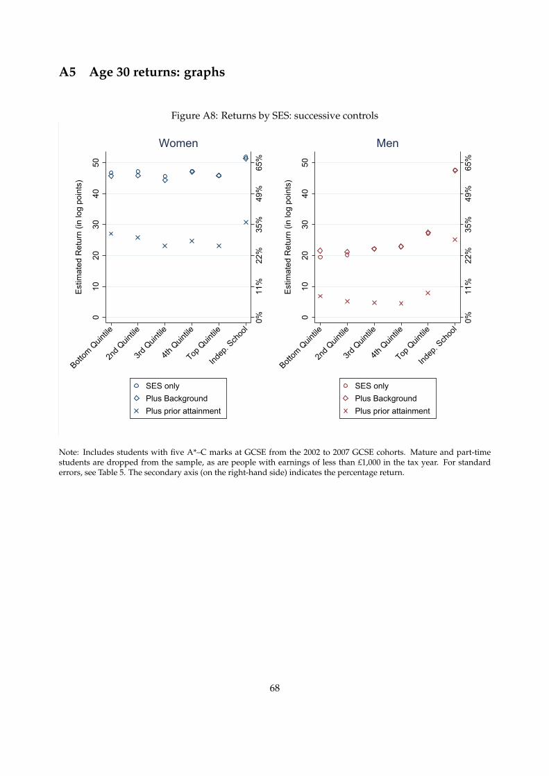
A5 Age 30 returns: graphs
Figure A8: Returns by SES: successive controls
0%11
%22
%35
%49
%65
%
010
2030
4050
Est
imat
ed R
etur
n (in
log
poin
ts)
Bottom
Quin
tile
2nd Q
uintile
3rd Q
uintile
4th Q
uintile
Top Q
uintile
Indep
. Sch
ool
SES onlyPlus BackgroundPlus prior attainment
Women
0%11
%22
%35
%49
%65
%
010
2030
4050
Est
imat
ed R
etur
n (in
log
poin
ts)
Bottom
Quin
tile
2nd Q
uintile
3rd Q
uintile
4th Q
uintile
Top Q
uintile
Indep
. Sch
ool
SES onlyPlus BackgroundPlus prior attainment
Men
Note: Includes students with five A*–C marks at GCSE from the 2002 to 2007 GCSE cohorts. Mature and part-timestudents are dropped from the sample, as are people with earnings of less than £1,000 in the tax year. For standarderrors, see Table 5. The secondary axis (on the right-hand side) indicates the percentage return.
68

Figure A9: Returns by ethnicity: successive controls
-33%
-18%
0%22
%49
%82
%
-40
-20
020
4060
Est
imat
ed R
etur
n (in
log
poin
ts)
Black C
aribb
ean
Chines
e
Black A
frican
Black O
ther
Whit
e Othe
rOthe
r
Indian
Whit
e Briti
sh
Bangla
desh
i
Pakist
ani
Ethnicity onlyPlus BackgroundPlus prior attainment
Women
-33%
-18%
0%22
%49
%82
%
-40
-20
020
4060
Est
imat
ed R
etur
n (in
log
poin
ts)
Black O
ther
Whit
e Briti
sh
Black C
aribb
eanOthe
r
Whit
e Othe
r
Bangla
desh
i
Black A
frican
Indian
Chines
e
Pakist
ani
Ethnicity onlyPlus BackgroundPlus prior attainment
Men
Note: Includes students with five A*–C marks at GCSE from the 2002 to 2007 GCSE cohorts. Mature and part-timestudents are dropped from the sample, as are people with earnings of less than £1,000 in the tax year. For standarderrors, see Table 6. The secondary axis (on the right-hand side) indicates the percentage return.
69

Figure A10: Returns by SES: impact of subject and institution choice, relative to highest SES quin-tile
-5%
0%5%
11%
16%
22%
-50
510
1520
Est
imat
ed R
elat
ive
Ret
urn
(in lo
g po
ints
)
Bottom
Quin
tile
2nd Q
uintile
3rd Q
uintile
4th Q
uintile
Indep
. Sch
ool
Relative ReturnWith subject controlsWith subject and HEI controls
Women
-5%
0%5%
11%
16%
22%
-50
510
1520
Est
imat
ed R
elat
ive
Ret
urn
(in lo
g po
ints
)
Bottom
Quin
tile
2nd Q
uintile
3rd Q
uintile
4th Q
uintile
Indep
. Sch
ool
Relative ReturnWith subject controlsWith subject and HEI controls
Men
Note: The top quintile of state-educated students is the omitted category. Includes students with five A*–C marks atGCSE from the 2002 to 2007 GCSE cohorts. Mature and part-time students are dropped from the sample, as are peoplewith earnings of less than £1,000 in the tax year. For standard errors, see Table 7. The secondary axis (on the right-handside) indicates the relative percentage return.
70

Figure A11: Returns by ethnicity: impact of subject and institution choice, relative to White British
-33%
-18%
0%22
%49
%
-40
-20
020
40
Est
imat
ed R
elat
ive
Ret
urn
(in lo
g po
ints
)
Whit
e Othe
r
Black C
aribb
ean
Black A
frican
Black O
ther
Indian
Pakist
ani
Bangla
desh
i
Chines
eOthe
r
Relative ReturnWith subject controlsWith subject and HEI controls
Women
-33%
-18%
0%22
%49
%
-40
-20
020
40
Est
imat
ed R
elat
ive
Ret
urn
(in lo
g po
ints
)
Whit
e Othe
r
Black C
aribb
ean
Black A
frican
Black O
ther
Indian
Pakist
ani
Bangla
desh
i
Chines
eOthe
r
Relative ReturnWith subject controlsWith subject and HEI controls
Men
Note: White British is the omitted category. Includes state-educated students with five A*–C marks at GCSE from the2002 to 2007 GCSE cohorts. Mature and part-time students are dropped from the sample, as are people with earningsof less than £1,000 in the tax year. For standard errors, see Table 8. The secondary axis (on the right-hand side) indicatesthe relative percentage return.
71
© IFS 2021
Reference: DFE-RR996
ISBN: 978-1-83870-244-1
The views expressed in this report are the authors’ and do not necessarily reflect those of the Department for Education.
For any enquiries regarding this publication, contact us at: [email protected] or www.education.gov.uk/contactus