The Response of the Antarctic Oscillation to Increasing

15 MAY 2003 1525C A I E T A L .

q 2003 American Meteorological Society

The Response of the Antarctic Oscillation to Increasing and StabilizedAtmospheric CO2

WENJU CAI AND PETER. H. WHETTON

CSIRO Atmospheric Research, Aspendale, Victoria, Australia

DAVID J. KAROLY

School of Mathematical Sciences, Monash University, Victoria, Australia

(Manuscript received 6 June 2002, in final form 14 October 2002)

ABSTRACT

Recent results from greenhouse warming experiments, most of which follow the Intergovernmental Panel onClimate Change (IPCC) IS92a scenario, have shown that under increasing atmospheric CO 2 concentration, theAntarctic Oscillation (AAO) exhibits a positive trend. However, its response during the subsequent CO 2 stabi-lization period has not been explored. In this study, it is shown that the upward trend of the AAO reversesduring such a stabilization period. This evolution of an upward trend and a subsequent reversal is present ineach ensemble of three greenhouse simulations using three versions of the CSIRO Mark 2 coupled climatemodel. The evolution is shown to be linked with that of surface temperature, which also displays a correspondingtrend and reversal, incorporating the well-known feature of interhemispheric warming asymmetry with smallerwarming in the Southern Hemisphere (smaller as latitude increases) than that in the Northern Hemisphere duringthe transient period, and vice versa during the stabilization period. These results indicate that once CO 2 con-centration stabilizes, reversal of the AAO trend established during the transient period is likely to be a robustfeature, as it is underpinned by the likelihood that latitudinal warming differences will reduce or disappear. Theimplication is that climatic impacts associated with the AAO trend during the transient period may be reversibleif CO2 stabilization is achieved.

1. Introduction

Analyses of observations over the last several decadessuggest that the leading mode of variability of mean sealevel pressure (MSLP) or 500-hPa geopotential height(Z500) modes in the mid- to high latitudes are the an-nular modes (Mo and White 1985; Mo and Ghil 1987;Karoly 1990, 1995; Kidson and Sinclair 1995; Watter-son 2000; Thompson and Wallace 1998, 2000; Hurrell1995). These modes have been referred to as the ArcticOscillation (AO) for the Northern Hemisphere (NH) andthe Antarctic Oscillation (AAO) for the Southern Hemi-sphere (SH). Thompson and Wallace (2000) and suggestthat the AAO and the AO are dynamically similar, andshow that there have been trends in these two modesover the past few decades with decreasing MSLP overthe polar latitudes and increasing pressure in midlati-tudes.

The forcing of the AO and AAO trends has receivedconsiderable attention. Thompson and Solomon (2002)and Sexton (2001) provide observational and modeling

Corresponding author address: Dr. Wenju Cai, CSIRO Atmo-spheric Research, PMB 1, Aspendale, Vic 3195 Australia.E-mail: [email protected]

evidence that the AAO trend is consistent with strato-spheric ozone loss over the past few decades. There hasalso been considerable interest in the response of thesemodes to greenhouse warming. Based on model simu-lations, Shindell et al. (1999) show that the observedAO trend can be attributed to greenhouse gas–inducedwarming, but they also find that such a response onlyexists in simulations with enhanced resolution in thestratosphere. Other studies indicate that the response ofthe AO varies significantly from one climate model toanother (Kushner et al. 2001). In Fyfe et al. (1999),which uses a relatively coarse resolution in the strato-sphere, the trend of the AO is simulated but is muchweaker than that in the Shindell et al. (1999) study. Inthe Geophysical Fluid Dynamics Laboratory warmingexperiments, which are of comparable resolution to theFyfe et al. (1999) integrations, there is no AO trend(Kushner et al. 2001). By contrast, the response of theAAO to increasing CO2 displays a robust definite up-ward trend in all transient greenhouse warming inte-grations.

Most of the warming experiments (e.g., Fyfe et al.1999; Kushner et al. 2001) have the atmospheric equiv-alent CO2 concentration that increases according to an

Unauthenticated | Downloaded 04/02/22 01:43 AM UTC

1526 VOLUME 16J O U R N A L O F C L I M A T E

Intergovernmental Panel on Climate Change (IPCC)scenario (Houghton et al. 1992; Michell et al. 1995;Haywood et al. 1997). All scenarios include a transientperiod, in which the equivalent CO2 increases at a spec-ified rate from a reference level. So far, only the responseof the AAO in the transient period has been studied.The subsequent behavior is yet to be explored. This isthe major focus of the present study. We analyze theresponse of the atmospheric circulation simulated by theCommonwealth Scientific and Industrial Research Or-ganisation (CSIRO) Mark 2 coupled GCM in threewarming runs all following the IPCC IS92a scenario.During the transient period, the equivalent CO2 increas-es from 1860 to 2083 when the CO2 triples the level ofthe pre-1860 level. All three warming runs then includea stabilization period of several centuries in which theCO2 is held at a constant, elevated 3 3 CO2 condition.

The rest of the paper is organized as follows. Afterdescribing the model and the experiments (section 2),we confirm the upward trend of the model AAO duringthe transient period and examine its subsequent behaviorduring the stabilization period, which shows a gradualreversal (section 3). We demonstrate that the responseof the AAO is linked with that of the Southern Ocean(section 4), which is in turn associated with the featureof interhemispheric warming asymmetry (e.g., Stoufferet al. 1989).

2. Model and model experiments

The CSIRO Mark 2 coupled model (Gordon andO’Farrell 1997) has a horizontal resolution of the R21spectral representation, or approximately 3.28 latitude3 5.68 longitude, in both the atmosphere and oceansubmodels. The atmospheric general circulation model(GCM) has nine vertical sigma levels. It includes a semi-Lagrangian treatment of water vapor transport, dynamicsea ice, and a bare soil and canopy land surface, as wellas standard parameterizations of radiation, cloud, pre-cipitation, and the atmospheric boundary layer. Theocean GCM has 21 vertical levels, and includes thescheme of Gent and McWilliams (1990), which param-eterizes the adiabatic transport effect of subgrid-scaleeddies, and replaces the nonphysical horizontal diffu-sivity as a means of stabilizing the model numerics. Theinclusion of the scheme results in a much improvedstratification leading to a major reduction in convectionat high southern latitudes. A detailed description of theimprovements has been given by Hirst et al. (2000) andthe improvement in the high-latitude Southern Oceanhas also been discussed by Cai et al. (2001).

The model experiments comprise three control cli-mate simulations [hereafter referred to as control 1(Hirst et al. 2000), control 2 (Matear et al. 2000; Matearand Hirst 2002), and control 3 (Bi et al. 2001)] usingthree versions of the coupled model, each run for atleast 600 yr of simulation. The three versions differ interms of the ocean spinup strategy and ocean and sea

ice parameterization. One difference lies in the forcingof the ocean spinup, in which the surface forcing fieldshave been modified such that the annual cycle of seasurface temperature (SST) and sea surface salinity overthe deep water formation regions are increasingly bettersimulated from control 1 to control 3 (Bi et al. 2001).This results in a progressively stronger deep-penetratingNorth Atlantic deep water and more realistic water massin the Southern Ocean from control 1 to control 3, yield-ing a stratification in control 3 that very closely matchesthe observed structure (see Bi et al. 2001 for furtherinformation). Another difference lies in the adjustmentof the sea ice model (O’Farrell 1998), in which thesensitivity of sea ice to ocean heat exchange is mademore realistic, increasing from control 1 to control 3(S. O’Farrell 2002, personal communication). As a re-sult, the sea ice amount in the control spinup state de-creases from control 1 to control 3.

Transient greenhouse warming runs are then con-ducted using the three versions of the coupled model inwhich the model is forced by increasing levels of green-house gases as observed (1880–1990) and according toIPCC scenario IS92a (1990–2100; Houghton et al.1992). The equivalent CO2 concentration doubles atabout year 2048 and triples at year 2083 from the pre-1880 level. Thus, in the model, the CO2 evolution rep-resents the changes of all anthropogenic greenhouse gas-es in the IS92a scenario. The three runs will be referredto as run 1 (Hirst 1999), run 2 (Matear et al. 2000;Matear and Hirst 2002), and run 3 (Bi et al. 2001), asthey start from control 1, control 2, and control 3, re-spectively.

This period in which CO2 increases is referred to asthe transient period. Thereafter, each warming run iscontinued for another several hundred years under aconstant 3 3 CO2 condition. This period is referred toas the stabilization period. At the time of analysis, theshortest run had been continued for about 400 yr underthe 3 3 CO2 condition. We shall compare the responseof the AAO in the three warming runs for the periodthat all three runs cover in common, that is, about 600yr. Bi et al. (2001) described the response of the South-ern Ocean overturning in run 3.

We apply empirical orthogonal function (EOF) anal-ysis to outputs of annual-mean anomaly/change fieldsof Z500 to identify major modes in all three of thecontrol and warming runs. We choose this variable be-cause it is a commonly used field, thus facilitating com-parison with results of other studies in terms of modessimulated in the control runs. For the three control runs,annual-mean anomalies are constructed from the long-term mean (averaged over a 600-yr period). For the threewarming runs the changes are calculated with referenceto the long-term mean of the respective control run.

In a recent study on projection of climate change ontomodes of atmosphere variability, Stone et al. (2001)identified variability patterns in the control run, and thenprojected climate change signals onto these patterns. In


15 MAY 2003 1527C A I E T A L .

FIG. 1. (a) EOF1 of Z500 anomalies in the SH domain, and (b)EOF1 and (c) EOF2 of Z500 anomalies in the global domain, allfrom control 1.

the present studies, we follow the approach of Fyfe etal. (1999) and apply EOF analysis directly to the chang-es, allowing responses to manifest as modes that maybe significantly different from those in the control run.If a mode from warming run outputs turns out to be thesame as one from the respective control run outputs, itmeans that the response manifests as a preexisting modein a natural way. In the event that a major response doesnot manifest as a preexisting mode, as is the case of theresponse of Z500 and SST, this approach provides anopportunity for such a response to be identified.

In one set of analyses, the domain is from the equatorto the South Pole, and in another the domain is global.Throughout the study we use covariance matrix EOF

analysis, and the gridpoint anomalies are neither areaweighted nor normalized, as in other studies of SH var-iability (e.g., Kiladis and Mo 1999; Fyfe et al. 1999).While such an analysis approach gives a stronger em-phasis on the high latitude, as variance there is greaterthan that at the low latitude in terms of Z500 or MSLPchanges, it may be appropriate as we are interested inthe AAO, which is mainly a mid- to high-latitude mode.To test the sensitivity to area weighting, we have con-ducted EOF analyses on area-weighted changes. We findthat there is little change in terms of the order of modesor the percentage each accounts for.

Major modes of Z500 in the SH domain in control 2have been recently examined by Cai and Watterson(2002). On interannual timescales, three modes are sig-nificant based on the North et al. (1982) criterion. Thefirst mode is the AAO, which has also been referred toas the high-latitude mode (e.g., Mo and White 1985;Mo and Ghil 1987; Karoly 1990, 1995; Kidson andSinclair 1995; Watterson 2000), or the zonally sym-metric or annular mode (e.g., Kidson 1988), reflectingthe feature of north–south out-of-phase variations be-tween the Antarctic and midlatitudes at all longitudes.The spatial pattern from one of the runs is shown inFig. 1a. The pattern correlation coefficients between theAAOs in the three control runs range between 0.97 and0.99. In the three control runs, the second mode is theso-called Pacific–South American (PSA) pattern (Moand Ghil 1987; Karoly 1989). The PSA is known to bestrongly influenced by tropical convection, which gen-erates wave trains extending across the South Pacificand South America (e.g., Berbery and Nogues-Paegle1993; Kiladis and Weickmann 1997; Mo and Higgins1997, 1998). In all three control runs, the third EOF isa mode with wavenumber-3 variability pattern in thelatitude band of 408–708S (e.g., Mo and White 1985;Kiladis and Mo 1999; Cai et al. 1999). In this study,we focus mainly on the response of the AAO.

In all three control runs, EOF1 in the global domainis the AAO (the pattern for one of the runs is shown inFig. 1b). These EOF1s account for approximately 18%of the total variance of each respective control run. Thepattern correlation coefficients between any two AAOmodes range between 0.97 and 0.98, and the patterncorrelation coefficient (in the SH domain) between Figs.1a and 1b reaches as high as 0.995. The correlationbetween the corresponding time series associated withFigs. 1a and 1b is virtually 1. In all three control runs,EOF2 in the global domain is the AO (the pattern forone of the runs is shown in Fig. 1c), each accountingfor approximately 14% of the total variance in eachrespective control run. The pattern correlation coeffi-cients between any two AO modes from the three con-trol runs range between 0.88 and 0.91.

3. EOF of response in the warming runsa. SH domain

In all three warming runs the first mode of Z500changes shows an increase in height everywhere as the



FIG. 2. EOF1 of Z500 changes from (a), (b), (c) the three warmingruns and (d) their corresponding time series. The pattern is not apredominant mode in its corresponding control run.

coupled system warms up (Figs. 2a–c). The pattern cor-relation between any two patterns of Figs. 2a–c rangesbetween 0.98–0.99, highlighting the similar, systematicresponse in the three warming runs. These EOF1s ac-count for 98.0%, 98.3%, and 97.9% of the total varianceof runs 1, 2, 3, respectively. All three EOF1 patternsdisplay a large increase over the Antarctic latitudes thanover lower latitudes. This is associated with the so-called sea ice–albedo positive feedback: in the high andpolar latitudes, the retreat of sea ice and/or snow greatlyreduces surface albedo, leading to enhanced solar ra-diation to the surface and larger warming there. Theevolution of the pattern (Fig. 2d) more or less followsthat of the prescribed CO2 increase. It features a steepupward trend as the model atmospheric CO2 increases(during the transient period) and then a continued butmoderate upward trend after the CO2 concentration levelis held constant (during the stabilization period). Wewill refer to this evolution as the ‘‘upward and continuedupward’’ response or ‘‘warming and continued warm-ing’’ response for the temperature field.

The warming trend shows significant differences fromone run to another, and the differences are particularlyprominent during the stabilization period; the warmingis greater in run 3 than in run 2 and smallest in run 1.A primary factor is that from control 1 to control 3, thestratification of the Southern Ocean is progressivelystronger. Thus, from run 1 to run 3, warming is pre-gressively more concentrated in the upper ocean. As aresult, the upper-ocean warming rate is greatest in run3, second in run 2, and smallest in run 1; in addition,sea ice reduction (in terms of percentage) is largest inrun 3. Through sea ice–albedo positive feedback, thedifference in sea ice response further enhances the dif-ference of the warming rate in the three runs.

The second EOF in all three runs is an AAO-like(Figs. 3a–c) mode. They account for 0.9%, 0.8%, and1.0% of the total variance of runs 1, 2, and 3, respec-tively. A statistical test using North et al’s (1982) cri-terion reveals that although they account for a smallpercentage of the total variance, these EOF2s are sta-tistically distinct from the EOF3s, which account for amaximum of 0.187% of the respective total variance.We have correlated each of the three patterns with theAAO pattern in the respective control run; the corre-lation coefficients range between 0.95 and 0.96, con-firming that these modes are indeed the AAO. The sys-tematic response of the coupled system is reflected bythe high pattern correlation coefficients between any twopatterns of Figs. 3a–c, which range between 0.98 and0.99. The evolution shows an upward trend during thetransient period, consistent with the findings of previousstudies (e.g., Fyfe et al. 1999; Kushner et al. 2001). Thecentral result here is the reversal and gradual recoveryduring the stabilization period to the level prior to theCO2 forcing. The time needed for the recovery appearsto be different from one run to another, again dependentupon the initial coupled climate state and the parameters


15 MAY 2003 1529C A I E T A L .

FIG. 3. EOF2 of Z500 changes from (a), (b), (c) the three warmingruns and (d) their corresponding time series. The 51-yr running meanversion of and the raw EOF time series are shown in (d). The patternis similar to that of the EOF1 of Z500 in the SH domain in itsrespective control run.

of the coupled system. We will refer to this evolutionas the ‘‘trend-reversing’’ response. The reversal of theAAO is also confirmed by linear trend maps of Z500fields for the two subperiods before and after year 2083,both being similar to the patterns of Figs. 3a–c.

The pattern of Z500 EOF1 also shows some merid-ional gradients in the southern midlatitudes. This raisesa question as to whether the AAO response also projectsonto the Z500 EOF1. To address this issue, we haveregressed, year by year, the Z500 change fields of awarming run onto the AAO pattern of each respectivecontrol run. This yields a time series of regression co-efficients for each run nearly identical to the time seriesof EOF2 in the respective warming run. This result sug-gests that little of the AAO response projects onto theZ500 EOF1. As will be clear, the forcing of the twoZ500 EOFs is quite different.

Some comments on the large difference in the vari-ance explained by Z500 EOF1 and EOF2 are in order.The large difference means that in terms of Z500 chang-es, EOF1 is by far the largest response. In the Fyfe etal. (1999) study, in which they applied EOF analysis onMSLP response, none of their EOF patterns show asstrong a direct greenhouse warming–related signal asthe Z500 EOF1 presented here. In our warming runs,EOF1 of the MSLP changes is also AAO-like (Figs. 4a–c), with a pattern similar to that of the Z500 EOF2changes, and accounts for about 45% of the total var-iance, consistent with the results of Fyfe et al. (1999).Thus, although the AAO-like response in Z500 appearsto be small (about 1% the total change as describedabove), at the surface it is the principal response pattern.The evolution (Fig. 4d) is also similar to that of Z500EOF2, with the trend-reversing feature. The second EOFof the MSLP (not shown), which corresponds to theZ500 EOF1, accounts for about 16% of the total vari-ances and the evolution shows an upward and continuedupward response. The fact that Z500 EOF1 show astronger warming signal than the MSLP EOF1 may in-dicate that MSLP EOF1 reflects a barotropic componentof the response, whereas the Z500 EOF1 represents abaroclinic component of the response with a strong ther-mal change in the lower troposphere.

The above results suggest that while the response canmanifest as a mode that is preexisting in the control run(Stone et al. 2001) the system can also generate a modeof response that is not preexisting. More importantly,the response that projects onto the preexisting mode hasa trend that exists only temporarily, and in the presentcase reverses once the CO2 concentration stabilizes,highlighting the importance of achieving a stabilizationof the atmospheric CO2 concentration.

To examine the coherence of changes of Z500 withthose of temperature, an EOF analysis on SST and/orsurface temperature changes has been conducted. Wefind that the above two modes of Z500 have corre-sponding modes in SST and surface temperature chang-es. The patterns of SST EOF1 in the three warming runs



FIG. 4. EOF1 and MSLP changes from (a), (b), (c) the three warm-ing runs and (d) their corresponding time series. The 51-yr runningmean version of and the raw EOF time series are shown in (d). Thepattern is similar to that of the EOF1 of MSLP in the SH domain inits respective control run.

(Figs. 5a–c) show that warming takes place everywhere,with a greater rate over high and polar latitudes (par-ticularly over sea ice regions) than over the low andmidlatitudes. We will refer to this mode as the polaramplification mode. The EOF1 of surface temperaturesshows a similar pattern, with generally larger warmingover land than over the oceans. The large warming inthe polar and high latitudes is a direct effect of the polaramplification, as described above. That such a responseis systematic is evident in the resemblance among Figs.5a–c. The correlation coefficients between any two pat-terns of Figs. 5a–c that are in the range of 0.98–0.99.The temporal evolution again shows a warming andcontinued warming trend. In the stabilization period,there are noticeable differences among the three runs,similar to that of the Z500 EOF1 (see Fig. 2d): the rateof warming is greatest in run 3, second in run 2, andlowest in run 1.

The patterns of the SST EOF2 (Figs. 6a–c) showweights of opposite polarity north and south of about458S, with maximum negative weights in the areas ofthe Ross and Weddell Seas. The pattern correlation co-efficients among them are again high, in the range of0.91–0.95. The patterns together with the temporal evo-lution (Fig. 6d) indicate that during the transient period,the warming rate decreases poleward; and there is arelative cooling trend in the latitudes south of approx-imately 458S. This is strongest in the convection regions.By ‘‘relative’’ we mean that the cooling trend takes placesimultaneously with the polar amplification warmingmode (EOF1), which shows a general warming trend.On balance, there is net warming. In other words, thecooling trend applies only after the warming trend as-sociated with EOF1 has been removed. For this reasonwe will interpret the EOF2 pattern as one with slowerwarming in the high latitudes than at lower latitudes,and the associated time series during the transient periodas a ‘‘relative cooling trend,’’ that is, relative to thegeneral warming trend associated with the polar am-plification mode.

There are several reasons for this spatial distributionof the SST EOF2. First, as noted in previous studies(Stouffer et al. 1989; Bryan et al. 1988), warming in theSH is smaller than in the NH because of the higher frac-tion of area covered by the ocean, which has a higherthermal inertia, highest along the latitude band of about458–658S, as it is completely covered by ocean. In section3b, we will show that this EOF2 pattern is part of theinterhemispheric asymmetry warming response proposedby Bryan et al. (1988) and Stouffer et al. (1989). Second,off the Antarctic coast, as sea ice melts, the SST is ‘‘reg-ulated’’ by the freezing temperature, also making it dif-ficult to warm. In such a background, it is the weakeningof the convective mixing, whereby less and less warmsubsurface water is brought to the surface, that is re-sponsible for the strong relative cooling trend. As willbe discussed in section 4, feedbacks between atmosphericfields of surface pressure, albedo, and surface temperature


15 MAY 2003 1531C A I E T A L .

FIG. 5. EOF1 of SST changes from (a), (b), (c) the three warmingruns and (d) their corresponding time series. The pattern is not apredominant mode in its respective control run.

FIG. 6. EOF2 of SST changes from (a), (b), (c) the three warmingruns and (d) their corresponding time series.



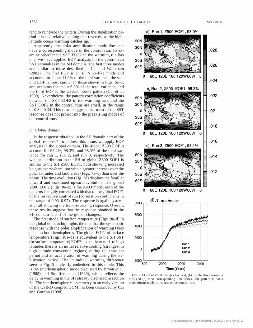
FIG. 7. EOF1 of Z500 changes from (a), (b), (c) the three warmingruns and (d) their corresponding time series. The pattern is not apredominant mode in its respective control run.

tend to reinforce the pattern. During the stabilization pe-riod it is this relative cooling that reverses, as the high-latitude ocean warming catches up.

Apparently, the polar amplification mode does nothave a corresponding mode in the control run. To ex-amine whether the SST EOF2 in the warming run hasone, we have applied EOF analysis on the control runSST anomalies in the SH domain. The first three modesare similar to those described in Cai and Watterson(2002). The first EOF is an El Nino–like mode andaccounts for about 11.8% of the total variance; the sec-ond EOF is most similar to those shown in Figs. 6a–c,and accounts for about 6.8% of the total variance; andthe third EOF is the wavenumber-3 pattern (Cai et al.1999). Nevertheless, the pattern correlation coefficientsbetween the SST EOF2 in the warming runs and theSST EOF2 in the control runs are small, in the rangeof 0.32–0.34. This result suggests that most of the SSTresponse does not project into the preexisting modes ofthe control runs.

b. Global domain

Is the response obtained in the SH domain part of theglobal response? To address this issue, we apply EOFanalysis in the global domain. The global Z500 EOF1saccount for 98.2%, 98.3%, and 98.3% of the total var-iance for run 1, run 2, and run 3, respectively. Theweight distribution in the SH of global Z500 EOF1 issimilar to the SH Z500 EOF1, both showing increasedheights everywhere, but with a greater increase over thepolar latitudes and land areas (Figs. 7a–c) than over theocean. The time evolution (Fig. 7d) displays the familiarupward and continued upward evolution. The globalZ500 EOF2 (Figs. 8a–c) is the AAO mode; each of thepatterns is highly correlated with that of the global EOF1of the respective control run (correlation coefficients inthe range of 0.93–0.97). The response is again system-atic, all showing the trend-reversing response. Overall,these results suggest that the response obtained in theSH domain is part of the global changes.

The first mode of surface temperature (Figs. 9a–d) inthe global domain highlights the fact that the systematicresponse with the polar amplification of warming takesplace in both hemispheres. The global EOF2 of surfacetemperature (Figs. 10a–d) is equivalent to the SH SST(or surface temperature) EOF2: in southern mid- to highlatitudes there is an initial relative cooling (strongest inhigh-latitude convection regions) during the transientperiod and an acceleration of warming during the sta-bilization period. The latitudinal warming differenceseen in Fig. 6 is clearly embedded in this mode. Thisis the interhemispheric mode discussed by Bryan et al.(1988) and Stouffer et al. (1989), which reflects thedelay in warming in the SH already discussed in section3a. The interhemispheric asymmetry in an early versionof the CSIRO coupled GCM has been described by Caiand Gordon (1998).


15 MAY 2003 1533C A I E T A L .

FIG. 8. EOF2 of Z500 changes from (a), (b), (c) the three warmingruns and (d) their corresponding time series. The 51-yr running meanversion of and the raw EOF time series are shown in (d). The patternis similar to a dominant mode (EOF1) in its respective control run.

FIG. 9. EOF1 of SST changes from (a), (b), (c) the three warmingruns and (d) their corresponding time series. The pattern is not apredominant mode in its respective control run.



FIG. 10. EOF2 of SST changes from (a), (b), (c) the three warmingruns and (d) their corresponding time series. The pattern is not adominant mode in its respective control run.

Examinations reveal that there is no interhemisphericmode of SST (or surface temperature) anomalies in thecontrol runs. Thus, the major response, in both EOF1and EOF2, of SST (or surface temperature) does notproject onto a preexisting mode. In analyses of changesduring the twentieth century, Cai and Whetton (2000,2001) found that in the tropical Pacific, the responsepattern of SST changes in ENSO–like. In the presentanalysis, the ENSO variability-like response appears asEOF3.

4. Discussion

a. The response of the AO

So far, we have not discussed the response of the AO.The EOF analysis of Z500 anomalies in the NH domainshows that the AO is the most dominant mode in allthree control runs. As discussed in section 2, the AO isalso the second most dominant mode in the global do-main. In the three warming runs, the global Z500 EOF3(Fig. 1c) is the AO mode (Figs. 11a–c). The patterncorrelation coefficients between this mode in the warm-ing run and the corresponding mode (Fig. 1c) in therespective control run are in the range of 0.88–0.91.However, the time series (Fig. 11d) shows that there islittle trend in the warming runs. It is not clear whetheror not the lack of an AO trend is due to model resolutionin the stratosphere. The main conclusion we arrive atis that in our model, besides the mode of the upwardand continued upward trend response, the remainingchange in Z500 projects mainly onto the AAO.

b. The dynamic environment for the AAO evolution

The trend-reversing evolution of both the AAO andthe temperature interhemispheric asymmetry mode sug-gest that the dynamics for these responses are linked.On the basis that only the ocean has a memory of time-scales of several centuries, we suggest that the trend-reversing evolution of the AAO (Z500 EOF2) is dy-namically determined by the temperature interhemi-spheric asymmetry mode. In the following we discussthe relationship between the AAO and temperature inthe control runs, and then comment on the dynamicsthat support this relationship in the warming runs.

The relationship between the AAO and surface tem-perature in control 2 (the respective control run of run2) has been recently examined by Cai and Watterson(2002). They showed that the temperature anomaly pat-tern associated with the AAO displays zonally sym-metric anomalies of opposing signs in the meridionaldirection (see their Fig. 3a). Over the latitudes whereheight (and MSLP) anomalies are positive, cloud coverdecreases, leading to an increased incoming radiativeheat flux and, hence, anomalously warm surface tem-peratures. Over the latitudes with negative height anom-alies: total cloud cover increases and less energy pen-


15 MAY 2003 1535C A I E T A L .

FIG. 11. EOF3 of Z500 changes from (a), (b), (c) the three warmingruns and (d) their corresponding time series. The 51-yr running meanversion of and the raw EOF time series are shown in (d). The patternis similar to a dominant mode (EOF2) in its respective control run.

etrates to the surface, leading to the development ofnegative surface temperature anomalies. This relation-ship exists in all three control runs.

The association of negative temperature weights withnegative height weights in the polar latitudes, and viceversa in the mid- to high latitudes (Figs. 3a–c and 6a–c), is therefore a continuation of the relationship thatexists in the control runs. During the transient period,decreasing MSLP over the relative cooling region (ap-proximately 458S poleward) provides favorable condi-tions for clouds and rainfall to increase. By contrast,north of the oceanic convective regions, the reverse istrue: cloud cover and rainfall decreases (the rainfall re-sponse will be discussed further in section 4c). Thislatitudinal setting reverses during the stabilization pe-riod in which warming in the Southern Ocean catchesup with a greater warming rate in the higher latitudesthan in the lower latitudes. This situation provides anappropriate dynamical environment in which the AAOreverses its trend and follows the evolution of the tem-perature EOF2.

The trend-reversing response of surface temperature,as manifested in Z500 EOF2, is not surprising given thewell-known response of interhemispheric warmingasymmetry. Indeed it is reassuring that such a featuremanifests as an EOF mode. The central result here isthat it shows a clear linkage to the AAO. The associatedtrend-reversing evolution implies that if CO2 stabili-zation is achieved, the trend of the AAO establishedduring the transient period is likely to reverse. This isbecause the latitudinal warming differences of theSouthern Ocean will eventually be eliminated.

c. Implications of the AAO evolution for climateimpacts

To discuss the issue of possible climate impacts ofthe model AAO response, it is appropriate to commenton the behavior of the observed AAO over the pastdecades and its possible linkage with other climate var-iables. Figures 12a and b show the AAO trend and pat-tern from an EOF analysis of monthly MSLP anomaliesfrom 1957 onward of the National Centers for Envi-ronmental Prediction (NCEP) reanalysis. A general up-ward trend is seen, as noted by previous studies. Thetrend is particularly steep in the late 1960s. This co-incides with a significant decrease in rainfall over south-west part of western Australia (SWWA; 1208E westwardand 1328S southward; Smith et al. 2000). There is vig-orous debate as to whether or not, and to what extent,the observed drying trend is induced by greenhousewarming.

The upward trend of the AAO means that the MSLPin the midlatitudes strengthens (Fig. 12b), providing alarge-scale condition for the decreasing rainfall. Figure12c depicts a map of correlation coefficients betweenthe time series of the AAO mode (Fig. 12a) and NCEPmonthly rainfall anomaly fields. It shows that when the



FIG. 12. (a) Time series and (b) pattern of EOF1 of monthly MSLPanomalies from NCEP reanalysis from 1957 onward. In (a), a 10-yrrunning mean curve is superimposed. (c) Map of correlation coef-ficients between the MSLP EOF1 time series and monthly rainfallanomalies. The contour interval is 0.1. (d) Time series of annual-mean rainfall over SWWA from a greenhouse warming run forced

←

by the IPCC IS92a scenario in which the atmospheric CO2 triplesthe initial value by year 2083 and is thereafter held at the elevated3 3 CO2 level; a 51-yr running mean curve is also displayed in theplot.

AAO is positive there is indeed a tendency for rainfallover SWWA to decrease. The implication is that if theobserved upward trend of the AAO is driven by green-house warming, it is likely that some of the drying trendis greenhouse induced as well.

Cai and Watterson (2002) showed that in the controlruns the above relationship between the AAO and rain-fall over SWWA is realistically simulated: when theAAO is positive, that is, with increased heights andMSLP in the midlatitudes, rainfall over SWWA tendsto decrease as a result of decreased westerly winds,bringing less frontal events to SWWA.

Figure 12d shows a time series of rainfall change overSWWA in one of the warming runs. Rainfall overSWWA experiences a decreasing trend during the tran-sient period, consistent with the observed decrease overthe past several decades, thus, supporting the argumentthat the observed drying trend may be partially inducedby global warming. In the stabilization period, rainfallthere undegoes a gradual recovery, taking some 500 yrto do so. The course of evolution is robust and is seenin all three warming runs.

It follows that climate impacts associated with theAAO trend established in the transient period may bereversible if CO2 stabilization is achieved. Whetton etal. (1997) applied EOF analysis to rainfall changes inrun 1. The EOFs 1 and 2 display the familiar upwardand continued upward and trend-reversing evolution,respectively. In many places, where rainfall responsesis predominantly controlled by EOF2, the trend estab-lished during the transient period reverses. The modeledrainfall response over SWWA, as shown in Fig. 12d, isone excellent example, and it highlights the importanceof achieving CO2 stabilization.

5. Conclusions

Recent studies have consistently shown that underincreasing atmospheric CO2 concentration, the AAOdisplays an upward trend. However, its response duringa subsequent CO2 stabilization period has not been ex-amined. In the present study, we show that the upwardtrend of the AAO reverses during such a stabilizationperiod. This course of evolution is present in all threemembers of the ensemble. The evolution is determinedby the latitudinal temperature gradients across the south-ern mid- to high latitudes embedded in the well-knowninterhemispheric warming asymmetry mode identifiedby previous studies. The fact that latitudinal warmingdifferences will eventually be eliminated once CO2 sta-bilization is achieved could therefore underpin the ro-


15 MAY 2003 1537C A I E T A L .

bustness of the AAO reversal. One important implica-tion of our result is that climatic impacts of greenhousewarming associated with the AAO trend during the tran-sient period may be reversible if CO2 stabilization isachieved. The above conclusions are based on the as-sumption that any AAO trend is forced by greenhousewarming alone. Therefore, these conclusions may notbe true in a situation in which the AAO trend is alsodriven by other forcings, as may to be the case over thepast several decades (Thompson and Solomon 2002).

Acknowledgments. This work was supported by theAustralian Greenhouse Office. We gratefully acknowl-edge the efforts of members of the Climate ModelingProgram and the Atmospheric Processes Program atCSIRO Atmospheric Research in developing the modelused in this study. We thank Paul J. Kushner and ananonymous reviwer for their helpful and insightful com-ments. We are grateful to Anthony Hirst and Dave Bifor permission to use their model outputs, and Prof. BillBudd for providing the computational resources to sup-port several of their integrations. Thanks also to DebbieAbbs and Anthony Hirst for reviewing our manuscriptbefore submission.

REFERENCES

Berbery, E. H., and J. Nogues-Paegle, 1993: Intraseasonal fluctuationsbetween the Tropics and extratropics in the Southern Hemi-sphere. J. Atmos. Sci., 50, 1950–1965.

Bi, D., W. F. Budd, A. C. Hirst, and X. Wu, 2001: Collapse andreorganization of the Southern Ocean overturning under globalwarming in a coupled model. Geophys. Res. Lett., 28, 3927–3930.

Bryan, K., S. Manabe, and M. J. Spelman, 1988: Interhemisphericasymmetry in the transient response of a coupled ocean–atmo-sphere model to a CO2 forcing. J. Phys. Oceanogr., 18, 851–867.

Cai, W., and H. B. Gordon, 1998: Transient responses of the CSIROclimate model to two different rates of CO2 increase. ClimateDyn., 14, 503–516.

——, and P. H. Whetton, 2000: Evidence for a time-varying patternof greenhouse warming in the Pacific Ocean. Geophys. Res. Lett.,27, 2577–2580.

——, and ——, 2001: Time-varying greenhouse warming patternand the tropical–extratropical circulation linkage in the PacificOcean. J. Climate, 14, 3337–3355.

——, and I. G. Watterson, 2002: Modes of interannual variability ofthe Southern Hemisphere circulation simulated by the CSIROclimate model. J. Climate, 15, 1159–1174.

——, P. G. Baines, and H. B. Gordon, 1999: Southern mid- to high-latitude variability, a zonal wavenumber-3 pattern, and the Ant-arctic Circumpolar Wave in the CSIRO coupled model. J. Cli-mate, 12, 3087–3104.

——, ——, and ——, 2001: Reply. J. Climate, 14, 1332–1334.Fyfe, J. C., G. J. Boer, and G. M. Flato, 1999: The Arctic and Antarctic

Oscillations and their projected changes under global warming.Geophys. Res. Lett., 26, 1601–1604.

Gent, P. R., and J. C. McWilliams, 1990: Isopycnal mixing in oceancirculation models. J. Phys. Oceanogr., 20, 150–155.

Gordon, H. B., and S. P. O’Farrell, 1997: Transient climate changein the CSIRO coupled model with dynamic sea ice. Mon. Wea.Rev., 125, 875–907.

Haywood, J., R. Stouffer, R. Wetherald, S. Manabe, and V. Ramas-wamy, 1997: Transient response of a coupled model to estimated

changes in greenhouse gas and sulfate concentrations. Geophys.Res. Lett., 24, 1335–1338.

Hirst, A. C., 1999: The Southern Ocean response to global warmingin the CSIRO coupled ocean–atmosphere model. Environ. Mod-el. Software, 14, 227–242.

——, S. P. O’Farrell, and H. B. Gordon, 2000: Comparison of acoupled ocean–atmosphere model with and without oceaniceddy-induced advection. Part I: Ocean spinup and control in-tegrations. J. Climate, 13, 139–163.

Houghton, J. T., B. A. Callander, and S. K. V. Varney, Eds.,1992:Climate Change 1992—The Supplementary Report to the IPCCScientific Assessment. Cambridge University Press, 200 pp.

Hurrell, J. W., 1995: Decadal trend in the North Atlantic Oscillation:Regional temperature and precipitation. Science, 269, 676–679.

Karoly, D., 1989: Southern Hemisphere circulation features associ-ated with El Nino–Southern Oscillation events. J. Climate, 2,1239–1252.

——, 1990: The role of transient eddies in low-frequency zonal var-iations of the Southern Hemisphere circulation. Tellus, 42, 41–50.

——, 1995: Observed variability of the Southern Hemisphere at-mospheric circulation. Natural Climate Variability on Decade-to-Century Time Scales, National Academy Press, 111–118.

Kidson, J. W., 1988: Indices of the Southern Hemisphere zonal wind.J. Climate, 1, 183–194.

——, and M. R. Sinclair, 1995: The influence of persistent anomalieson Southern Hemisphere storm tracks. J. Climate, 8, 1938–1950.

Kiladis, G. N., and K. M. Weickmann, 1997: Horizontal structureand seasonality of large-scale circulation associated with sub-monthly tropical convection. Mon. Wea. Rev., 125, 1997–2013.

——, and K. C. Mo, 1999: Interannual and intraseasonal variabilityin the Southern Hemisphere. Meteorology of the Southern Hemi-sphere, Meteor. Monogr., No. 35, Amer. Meteor. Soc., 307–336.

Kushner, P. J., I. M. Held, and T. L. Delworth, 2001: Southern Hemi-sphere atmospheric circulation response to global warming. J.Climate, 14, 2238–2249.

Matear, R., A. C. Hirst, 2002: Long term changes in dissolved oxygenconcentrations in the ocean caused by protracted global warming.Geochem. Geophys. Geosyst., in press.

——, ——, and B. I. McNeil, 2000: Changes in dissolved oxygenin the Southern Ocean with climate change. Geochem. Geophys.Geosyst., 1, 2000GC00086. [Available online at http://www.g-cubed.org/.]

Michell, J., T. Johns, J. Gregory, and S. Tett, 1995: Climate responseto increasing levels of greenhouse gases and sulphate aerosols.Nature, 376, 501–504.

Mo, K. C., and C. H. White, 1985: Teleconnections in the SouthernHemisphere. Mon. Wea. Rev., 113, 22–37.

——, and M. Ghil, 1987: Statistics and dynamics of persistent anom-alies. J. Atmos. Sci., 44, 877–901.

——, and R. W. Higgins, 1997: Planetary waves in the SouthernHemisphere and linkages to the tropics. Harry van Loon Sym-posium, Studies in Climate, Part II. NCAR Tech. Note TN-4331Proc., 290 pp.

——, and ——, 1998: The Pacific–South American modes and thetropical convection during the Southern Hemisphere winter.Mon. Wea. Rev., 126, 1581–1596.

North, G. N., T. L. Bell, R. F. Cahalan, and F. J. Moeng, 1982:Sampling error in the estimation of empirical orthogonal func-tions. Mon. Wea. Rev., 110, 699–706.

O’Farrell, S. P., 1998: Sensitivity study of a dynamical sea icemodel: The effect of the external stresses and land boundaryconditions on ice thickness distribution. J. Geophys. Res., 103,15 751–15 782.

Sexton, D. M. H., 2001: The effect of stratospheric ozone depletionon the phase of the Antarctic Oscillation. Geophys. Res. Lett.,28, 3697–3700.

Shindell, D. T., R. L. Miller, G. A. Schmidt, and L. Pandolfo, 1999:Simulation of recent northern winter climate trends by green-house-gas forcing. Nature, 399, 452–455.



Smith, I. N., P. McIntosh, T. J. Ansell, C. J. C. Reason, and K.McInnes, 2000: Southwest western Australian winter rainfall andits association with Indian Ocean climate variability. Int. J. Cli-matol., 20, 1913–1930.

Stone, D. A., A. J. Weaver, and R. J. Stouffer, 2001: Projection ofclimate change onto modes of atmospheric variability. J. Cli-mate, 14, 3551–3565.

Stouffer, R. J., S. Manabe, and K. Bryan, 1989: Interhemisphericasymmetry in climate response to a gradual increase of atmo-spheric CO2. Nature, 89, 571–586.

Thompson, D. W. J., and J. M. Wallace, 1998: The Arctic Oscillation

signature in the wintertime geopotential height and temperaturefields. Geophys. Res. Lett., 25, 1297–1300.

——, and ——, 2000: Annular modes in the extratropical circulation.Part I: Month-to-month variability. J. Climate, 13, 1000–1016.

——, and S. Solomon, 2002: Interpretation of recent Southern Hemi-sphere climate change. Science, 296, 895–899.

Watterson, I. G., 2000: Southern midlatitude zonal wind vacillationand its interaction with the ocean in GCM simulations. J. Cli-mate, 13, 562–578.

Whetten, P. H., Z. Long, and I. N. Smith, 1997: Comparison of sim-ulated climate change under transient and stabilised CO2. BMRCRes. Rep. 69, Melbourne, Victoria, Australia, 96 pp.


Documents

The Response of the Antarctic Oscillation to Increasing