Claremont CollegesScholarship @ Claremont

CMC Senior Theses CMC Student Scholarship

2013

The Residential Real-Estate Industry in India:Investigating Evidence for an Asset BubbleNikhita NarendranClaremont McKenna College

This Open Access Senior Thesis is brought to you by Scholarship@Claremont. It has been accepted for inclusion in this collection by an authorizedadministrator. For more information, please contact scholarship@cuc.claremont.edu.

Recommended CitationNarendran, Nikhita, "The Residential Real-Estate Industry in India: Investigating Evidence for an Asset Bubble" (2013). CMC SeniorTheses. Paper 761.http://scholarship.claremont.edu/cmc_theses/761

CLAREMONT MCKENNA COLLEGE

THE RESIDENTIAL REAL-ESTATE INDUSTRY IN INDIA: INVESTIGATING

EVIDENCE FOR AN ASSET BUBBLE

SUBMITTED TO

PROFESSOR DARREN FILSON

AND

DEAN NICHOLAS WARNER

BY

NIKHITA NARENDRAN

FOR

SENIOR THESIS

FALL 2013

December 2nd

, 2013

Abstract

The objective of this thesis is to examine the differences in residential property

prices across different cities in India. Soaring prices have led to increasingly unaffordable

property prices in large metropolitan cities. As a result, there has been academic

discourse about the existence of a housing bubble in recent years. In the past, empirical

research has focused on national level trends due to a lack of city-level data. I investigate

the city-fixed effects on growth in house prices across fifteen different cities. Although

different empirical models suggest different conclusions about these effects, point

estimates suggest above-normal growth in house prices in Delhi for the period 2009-

2013.

1

Acknowledgements

I would like to thank my Senior Thesis Reader, Professor Darren Filson for his

support and engagement at every stage of this project. His guidance and feedback have

been crucial to writing this paper. I would like to thank Professor Mitch Waratchka for

guiding my research and methodology. Finally, I would like to thank my family and

friends for their unwavering support in all my endeavors.

2

Table of Contents

I. Introduction .................................................................................................................. 3

II. Literature Review ....................................................................................................... 6

IV. Dynamics of the Housing Market ........................................................................... 12

VI. Data ......................................................................................................................... 14

VII. Methodology .......................................................................................................... 18

VIII. Results .................................................................................................................. 20

IX. Conclusion .............................................................................................................. 24

X. References ................................................................................................................ 26

XI. Appendix ................................................................................................................. 29

3

I. Introduction

The real-estate industry is inextricably linked to socio-economic growth and

development. Increasing the availability and affordability of housing can improve the

quality of life for citizens, and the overall development of infrastructure improves

productivity within the economy. House prices also indirectly impact macroeconomic

health through the wealth effect: as house prices rise, home-owners feel wealthier and are

likely to increase consumption and boost aggregate demand (Calomiris, Longhofer, &

William, 2012).

The residential real-estate industry in India is complex and dynamic. Varying

economic and demographic characteristics across the country result in differences in the

housing markets in different cities. While soaring prices have led to speculation about a

housing bubble in large cities like Mumbai and Delhi, prices in tier-II and tier-III cities

such as Kochi and Hyderabad have remained relatively stagnant (NHB, 2013). Demand

for housing has increased in recent years due to rising per capita incomes, the increasing

penetration of housing finance, and increasing population density in urban areas. The

growing middle class, expected to grow from 224 million to 583 million by 2025, has

added to existing pressure on the demand for housing (Mustafi, 2013).

The Indian government is faced with several challenges as it attempts to stabilize the

housing market and increase accessibility to affordable housing. In light of rising

inflation and twin current account and fiscal deficits, the government has attempted to

increase liquidity and encourage household saving during 2012-13 by pursuing tight

monetary policy (Moneycontrol, 2013). Consequently, investment growth in the

industrial sector experienced a slowdown and contributed - along with a slowdown in the

4

industrial, agriculture and services sector- to a decline in GDP growth to 5 percent in

2012-13 (Moneycontrol, 2013) . Residential real-estate markets have followed suit, with

Mumbai and Delhi experiencing a 0.5 percent and 1.5 percent fall in prices respectively,

and cities like Chennai and Kolkata dropping by 2.3 percent and 4.1 percent respectively

(Kumar, 2013).

The objective of this paper is to examine how the macroeconomic environment and

monetary policy impact trends in house prices in different cities. I will test the hypothesis

that house prices in certain metropolitan cities such as Delhi and Mumbai have seen

above-normal growth rates in recent years. My hypothesis is motivated by literature

speculating about existence of a housing bubble in these cities (Anand, 2010).

In order to test my hypothesis I construct a panel of fifteen cities for fifteen quarters

since 2009. I use a fixed effects model to account for omitted variables that cannot be

measured and attempt to determine whether large metropolitan cities display positive

fixed effects in house price growth. I then investigate whether the slowdown of the Indian

economy since 2010-11 has impacted the growth of house prices (Schaffer, 2013).

In the past, literature pertaining to residential real-estate markets in India has focused

on national level house prices as well as analysis of certain cities such as Mumbai

(Gandhi, 2000). However, the vast majority of this literature is outdated. Since 2007, the

National Housing Bank has published a house price index (HPI) called the Residex for

fifteen cities in India and my objective is to use this to demonstrate city-wise variation in

house markets while controlling for economy-wide interest rates.

5

My results suggest that the real interest rate is statistically significant, and negatively

related to change in house prices as basic economic theory would suggest (Mankiw,

2011). Although point estimates suggest that four out of the six metropolitan cities

(including Delhi and Mumbai) display above-normal increases in house prices, different

ways of computing the standard errors suggest different conclusions about the

significance of these results.

There are two major qualifications for the empirical analysis I present in this thesis.

Firstly, that I use 2007 as a base year. By this time, prices in metropolitan cities had

already surpassed those in other cities. Prior to 2009, both Delhi and Mumbai had

experienced periods of rapid growth in house prices1. As a result, the available data does

not capture the full extent of above-normal house price growth rate experienced in these

cities. Secondly, urbanization and demographic trends that contribute to the pressure on

housing markets could not be accounted for in this dataset due to the fact that census data

is reported in five year intervals and because economic data used to construct my

independent variables is unavailable at the city-level.

1 Figure 3

6

II. Literature Review

The literature pertaining to the real-estate market in India consists primarily of reports

published by the Reserve Bank of India and by the National Housing Bank. The Report

on Trend and Progress of Housing in India (2012) describes the dynamics of the housing

market in India. The National Housing Bank was established by the Reserve Bank of

India in 1988 in order to promote private real estate acquisition. The NHB is also

responsible for regulating and refinancing social housing programs. In its yearly reports,

the organization summarizes the issues concerning housing in India. The primary focus is

the availability of affordable housing and some of the impediments include

overpopulation of certain areas, the lack of affordable finance, infrastructure and

regulatory hurdles. Urbanization has led to demographic changes across the country.

According to census data, the percentage of population living in urban areas rose from 28

to 31 percent between 2006 and 2011, and is estimated to have risen further in recent

years (NHB, 2012).

Publications by the Reserve Bank of India focus on the deployment of housing

finance in India. Mohanty (2013) discusses the future of housing finance in light of the

demand-supply gap, favorable demographics and increasing urbanization. He asserts the

need to preserve financial stability along with attempts to increase the availability of

housing finance and presents evidence from Reinhard and Rogoff (2009) to illustrate that

the six major banking crises in advanced economies since the mid-1970s were associated

with a housing bust. Mohanty compares the housing market in India with the housing

market in the US, observing several crucial differences such as “the predominance of new

construction and first time ownership” in India. Yet, he suggests it is important to apply

7

lessons learned from the sub-prime crisis in order to prevent a financial crisis due to a

housing bust.

Gandhi (2012) describes the pressure on house prices in Mumbai over recent years.

As the city became a center for economic and commercial activities, Mumbai

experienced a rapid growth in population leading to distortions in the housing markets in

India that impede the availability of affordable housing. The paper illustrates a mismatch

between household income and house prices evidenced by the fact that “at the present

income distribution and institutional rates, only 5-6 percent of households can afford a

house in Mumbai” (Gandhi, 2012). It also illustrates a violation of the household’s stock

and flow principle that is essential for equilibration in the housing sector (Lipsey &

Harbury, 2004). When measured against the distance from a city’s central business

district, most cities in the world have a downward sloping Floor Space Index (FSI)

(Bertraud, 2010). However, property prices in Mumbai violate the principle that there is a

flat FSI line against distance from the city center. In these big cities, house developers

cater to a small proportion of the population – the rich elite – by focusing on the

construction of luxury housing (Gandhi, 2012). Although Gandhi focuses on Mumbai in

his paper, he suggests that most Indian cities face “issues of infrastructure, slum

proliferation and inefficient urban land management” in the housing sector.

Several pieces of economic literature describe the relationship between residential

real-estate and the macroeconomy. Goodheart & Hoffman (2007) examine the effects of

house prices on the macroeconomic environment to demonstrate how a contraction in

house prices can have “a severe contractionary effect on output” and that house prices

reflect changes is beliefs and economic speculation. DiPasquale & Wheaton (1996)

8

distinguish between a micro and a macro approach to real estate markets. The micro

approach emphasizes the importance of structural and geographic factors in determining

house prices. Wheaton suggests that structural characteristics such as the level of

development affect the willingness to pay across different locations. The macro approach

deals with the effect of high level forces such as growth, industry and competitiveness on

real-estate markets in different cities.

Case and Shiller (2004) discuss the role of expectations in causing a bubble in the

housing market, identifying this as a situation in which “excessive public expectations of

future price increases cause prices to be temporarily elevated.” The rapid growth in house

prices that have been seen across several cities in India is considered to be the first sign

of a bubble. Yet, this is not conclusive evidence for the existence of a bubble. The extent

to which changes in macroeconomic fundamentals, including incomes and interest rates,

explain these growth rates can give us insight into whether it is appropriate to speculate a

bubble.

Joshi (2006) examines preliminary evidence to suggest the existence of an asset

bubble in the Indian housing market. He used a structural VAR model proposed by

Blanchard and Quah (1989) to study the shocks to house prices that can be attributed to

the monetary variables and income growth. The paper concludes that the Indian housing

market was well equilibrated and that the risk of a bubble was not significant at this time.

Another important finding was that monetary policy, specifically the interest rate, was the

single most important determinant of the future growth of the housing market.

9

III. Macroeconomic Overview

India, the world’s fourth-largest economy with a population of 1.2 billion, is still in

crucial stages of economic development. Over the past decade, the country has seen

tremendous growth and change. According to the Macro-economic Framework

Statement issued by the Ministry of Finance, The decadal average growth rate 2003-04 to

2012-13 was reported at 7.9 percent, with several consecutive years of 9 percent growth

rates before the financial crisis of 2008. Since 2011-12 the Reserve Bank of India (RBI)

has been using tight monetary policy to deal with uncertainty in the global economy. As a

result, industrial growth has slowed in recent years and gross domestic product at factor

cost was reported at 5 percent for 2012-13 (Ministry of Finance, 2013). Simultaneously,

inflation has been accelerating with Wholesale Price Inflation (WPI) rising to 6.46

percent in September, 2013 and inflation rising to 9.84 percent (Kala, 2013). The Indian

economy has been running twin deficits with a fiscal deficit of US$147 billion and a

current account deficit at 4.6 percent of GDP (Ministry of Finance, 2013). The adoption

of tight monetary policy has resulted in a decline in quarterly growth rate of GDP and

declining government revenues from the industrial sector. Furthermore, negative export

growth rates have led to unfavorable balance of payments. Simultaneously, the Indian

Rupee has been on a downward trend since August 2011 and hit an all-time low of INR

68.80 against the US Dollar in August 2013 (Ministry of Finance, 2013).

The real-estate industry plays a crucial role within the dynamic landscape of the

Indian economy. In 2013, it is estimated that the real-estate market contributed to 6.3

percent of GDP (IBEF, 2013). This sector is projected to generate 7.6 million jobs in this

period, and over 17 million by 2025 (IBEF, 2013). In India, housing ranks fourth in terms

10

of the multiplier effect on the economy and third in terms of its linkages to ancillary

industries (NHB, 2012). It is the second largest employment generator and provides jobs

to approximately 33 million people (NHB, 2012). Rising incomes, favorable

demographics, urbanization and inflows of foreign investments has led to an increase in

the demand for housing which has not been met with supply. On average, property values

have quadrupled in the last decade with rising property prices in urban areas and the

housing shortage is estimated at approximately 19 million households (Srivastava, 2013;

KPMG, 2012).

Over the past decade there has been a widespread expectation of rising property

prices and speculation of a housing bubble in large metropolitan cities. It had been

common for middle class buyers to buy houses with the intent of selling them a few years

later for a 15 -20 percent gain. In metropolitan cities like Mumbai and Delhi, houses that

are in the process of being constructed were sold for less than what the builder would sell

them for, to buyers who plan on re-selling them in the near future. Yet, according to the

Ministry of Housing and Urban Poverty Alleviation approximately 11.09 million homes

in urban areas remain empty (KPMG, 2012). Sellers have been holding out in hope that

property prices will continue to appreciate. As a result, houses have become increasingly

unaffordable for the middle class buyer.

The recent downturn in the Indian economy has led to an overall slump in the housing

market. The House Price Index (HPI) has been on a downward trend in 22 out of the 26

cities monitored by the National Housing Bank (NHB, 2013). Investor-driven real estate

markets such as certain areas in Delhi and Mumbai have seen more than 10 percent fall in

prices due to a slowing liquidity, a lack of buyers and a decline of investor confidence in

11

the property market (Chadha, 2013). Against the backdrop of falling prices, the question

about a housing bubble and a potential housing bust has become increasingly pertinent.

12

IV. Dynamics of the Housing Market

Two industries closely linked to the housing market in India are the housing finance

industry and the construction industry. The market for home loans is expected to grow at

a ~17 percent CAGR over the next five years due to increase in the number of

transactions, a higher loan to value (LTV) ratio and increasing property prices (Rupee

Manager, 2013). The two major players that operate within this space are Housing

Finance Companies (HFCs) and Scheduled Commercial Banks (SCBs). While HFCs are

regulated by the National Housing Bank (NHB), SCBs are regulated by the Reserve Bank

of India. While SCBs dominated the market in the late 1990s due to the prevalence of

low interest rates, rising incomes and stable property prices, the current market share is

split almost equally between the two (Rupee Manager, 2013). The main difference

between these institutions is their source of funds, with banks depending on their own

equity reserves and HFCs depending on loans from banks, financing from the NHB, fixed

deposits from the public and borrowing through bonds and debentures in addition to their

own equity reserves (Rupee Manager, 2013). In recent years, the availability of

affordable home loans at low interest rates has been increasing. The Indian government

has played a role in this, by offering tax concessions to boost demand for housing. As a

result, the penetration of housing finance has reached an estimated 38 percent in urban

areas (Prem, 2012).

In spite of the recent growth in demand for housing, there are several constraints to

real estate development. Firstly, there is a shortage of land in urban areas with growing

population densities as a result of urbanization. The shortage of land is exacerbated by

the existence of the Urban Land Ceiling Act passed in 1976 that restricts the land

available for construction and development (KPMG, 2012). In 2007, the state of

13

Maharashtra repealed this Act, releasing close to 3,000 acres for development in Mumbai

(CNN IBN, 2007). Nevertheless, inefficient land use by the public sector continues to

limit its availability.

Secondly, cumbersome regulation lengthens the process and increases the cost of

housing development. Estimates suggest that real estate developers need to pass

approvals through 150 tables in 40 government departments. Delays in approvals add 25-

30 percent to project costs and it currently takes two to three years for a developer to

begin construction after purchasing land (KPMG, 2012).Lastly, rising construction costs

further impede the development of real estate. While land forms the largest component of

premium residential real-estate projects, construction costs are 50 to 60 percent of the

selling price for affordable housing (KPMG, 2012).

14

VI. Data

My approach is modeled after a research paper published by the Reserve Bank of

India (Joshi, 2006). In order to investigate the existence of a housing price bubble, Joshi

employs a structural VAR model proposed by Blanchard and Quah (1989) to study the

impact of monetary variables and income growth on the housing price shocks in India.

My objective is to test the extent to which the macroeconomic fundamentals support the

growth rate of national level house prices. I build on Joshi (2006) to test the hypothesis

that there is a city-fixed effect that impacts the relationship between the macroeconomic

fundamentals and the growth in house prices. Additionally, I use Joshi (2006) to inform

the use of appropriate proxies for residential real-estate market data that is not available

on a quarterly basis. I construct a panel of fifteen tier-I and tier-II cities over 15 quarters

since 2009 using time series data published by the Reserve Bank of India.

Dependent Variable

In order to assess whether house price growth is supported by the macroeconomic

fundamentals, I use the quarterly growth in house prices for each city as my dependent

variable: hg. This growth rate is based on an Index constructed by the National Housing

Bank (NHB) called the Residex or the House Price Index (HPI). The Residex is

calculated using primary data on house prices from real-estate agents and housing finance

companies using a weighted average method. The quarterly growth rate is calculated as:

(1)

15

Independent Variables

My dependent variables include measures and proxies of macroeconomic

fundamentals expected to impact growth in house prices.

real_ir represents the quarterly real interest rates. Modeled after the RBI report,

the weighted-average call money rate is used as a proxy for the interest rate on home

loans because housing finance companies and scheduled commercial banks change their

rates in sync with the short term money market rates. infl_rate represents the quarterly

levels of Consumer Price Index to reflect changes in overall price inflation. This interest

rate is adjusted for the change in inflation during each quarter, and therefore represents

the real interest rate:

(2)

creditg is a proxy for quarterly growth in credit deployment to the housing sector.

It is a measure of non-food credit deployment, of which housing credit forms a large

proportion (Joshi, 2006) and is calculated as follows:

(3)

gdpg represents the quarterly growth in India’s Gross Domestic Product and is

used as a proxy for overall growth in demand. However, given that the housing sector

forms a significant proportion of GDP, it is difficult to determine whether GDP growth is

16

representative of changes in overall demand or reflective of growth in construction in the

real-estate sector.

(4)

The following table displays the summary statistics for each variable:

Variable Obs Mean Std. Dev Min Max

hg 210 2.67% 7.67% -16.80% 31.11%

real_ir 210 4.67% 1.86% 1.47% 8.26%

gdpg 210 2.34% 5.46% -6.85% 9.71%

creditg 210 4.27% 1.68% 0.81% 7.17%

infl_rate 210 2.23% 5.04% 0% 4.15%

Limitations

Several constraints limited the number and types of variables I chose to include.

Firstly, my variables reflect changes in macroeconomic fundamentals rather than city-

level economic fundamentals due to the unavailability of city-level data. A more

appropriate test for the existence of a bubble would measure the deviation of house prices

from economic demand and supply within the city. Given that different cities in my

sample are in different stages of economic development, they have different levels of

income, financial penetration and residential construction. Secondly, the model could be

improved by including a variable related to housing construction as a proxy for the

supply side of the residential real-estate industry.

17

Thirdly, the data captures only part of the time period during which there has been

speculation about a housing bubble. A more appropriate model would include data

extending to the early 2000s when property prices in big metropolitan cities first began to

soar2.

Lastly, although the goal of this thesis is to investigate the housing bubble

hypothesis by testing for deviation from macroeconomic fundamentals, the Case-Shiller

method of comparing growth in house prices with growth in rental yields could provide

more conclusive results about the existence of a property bubble. One of the major

qualitative motivations for my hypothesis is that Indian home-buyers are often more

concerned with purchasing houses as investments than rental gains. A model

investigating the extent to which growth in home prices can be explained by growth in

rental yields, reflecting demand for living space could provide valuable insights into the

existence of a bubble.

2 Figure 2

18

VII. Methodology

My starting point to investigate the relationship between macroeconomic

fundamentals and growth in house prices across different cities is a fixed effects model

assuming heteroscedasticity-robust standard errors3:

: the unknown intercept for each entity (i=1…n)

: the dependent variable (i= entity and t= time)

: the coefficient for the independent variables

: the error term

I construct binary variables for each city and each time period in order to investigate city-

fixed effects in the growth of house prices. I test the effects of grouping Delhi and

Mumbai under the variable large_city in order to investigate whether there is a difference

in the way that house prices in these markets respond to a change in macroeconomic

fundamentals. Additionally, I include the independent binary variable time1 to test for an

effect on house price growth in the period of macroeconomic slowdown in FY11-12.

I modify my model based on preliminary insights into the explanatory power of

my economic variables. I graph the residuals on the heteroscedasticity-robust fixed

effects model in order to look for autocorrelation and consider the effects of clustering

the cross-sectional residuals.

Finally, I investigate the effects of imposing structure on the residuals by using a

panel-corrected standard errors (PCSE) model and a First Order Autoregressive (AR(1))

3 the variance of the residuals is not consistent across all observation points

19

model to test the hypothesis that the residual is related to the residual in the previous

period, across cities at each point in time.

20

VIII. Results

Table 1 displays the results of the heteroscedasticity-robust fixed effects

regression. The coefficients can be interpreted as follows:

This model attempts to explain the variation of , the house price growth for

city in time period that is explained by the real interest rate, inflation rate, and GDP

growth rate since the previous quarter4. The growth in real interest rate, real_ir and the

growth in GDP, gdpg are statistically significant at 5 percent level. The coefficient on

real_ir suggests that a 0.679 percentage point decline in the real interest rate leads to an

increase in the growth rate of house prices by 1 percentage point.

The negative coefficient on gdpg suggests that a 0.212 percentage point decline in

GDP quarterly growth rate is associated with a 1 percentage point increase in the

quarterly growth rate of house prices. This result is counter-intuitive if we consider GDP

to be a proxy for demand. However, there are two plausible explanations for the result.

Firstly, it might suggest that GDP growth is a closer proxy for the supply-side of

residential real estate. Therefore, a decline in supply leads to an increase in house prices.

Alternatively, this negative relationship can be representative of a deviation of house

prices from the macroeconomic fundamentals if the growth of house prices is unrelated to

aggregate demand within the country. The negative coefficient on infl_rate reinforces the

latter explanation by suggesting that growth in house prices is not positively correlated

with overall inflation. The adjusted of this model is 0.023, indicating that only 2.3

percent of the variation in is explained by the model.

4

21

Table 2 displays the results of including a binary variable which takes a value of

1 in the period before the economic slowdown of 2010-11 (period1) in the original

regression. period1 is statistically significant at the 1 percent level and gdpg at the 5

percent level according to this model.

The positive coefficient on period1 suggests that quarterly growth in house prices

was higher in the period before 2011-12. gdpg is again found to be statistically significant

negatively correlated with house price growth. The adjusted indicates that this model

explains 6 percent of variation in . In other words, the macroeconomic variables

included in this model account only for 6 percent of the quarterly growth in house prices.

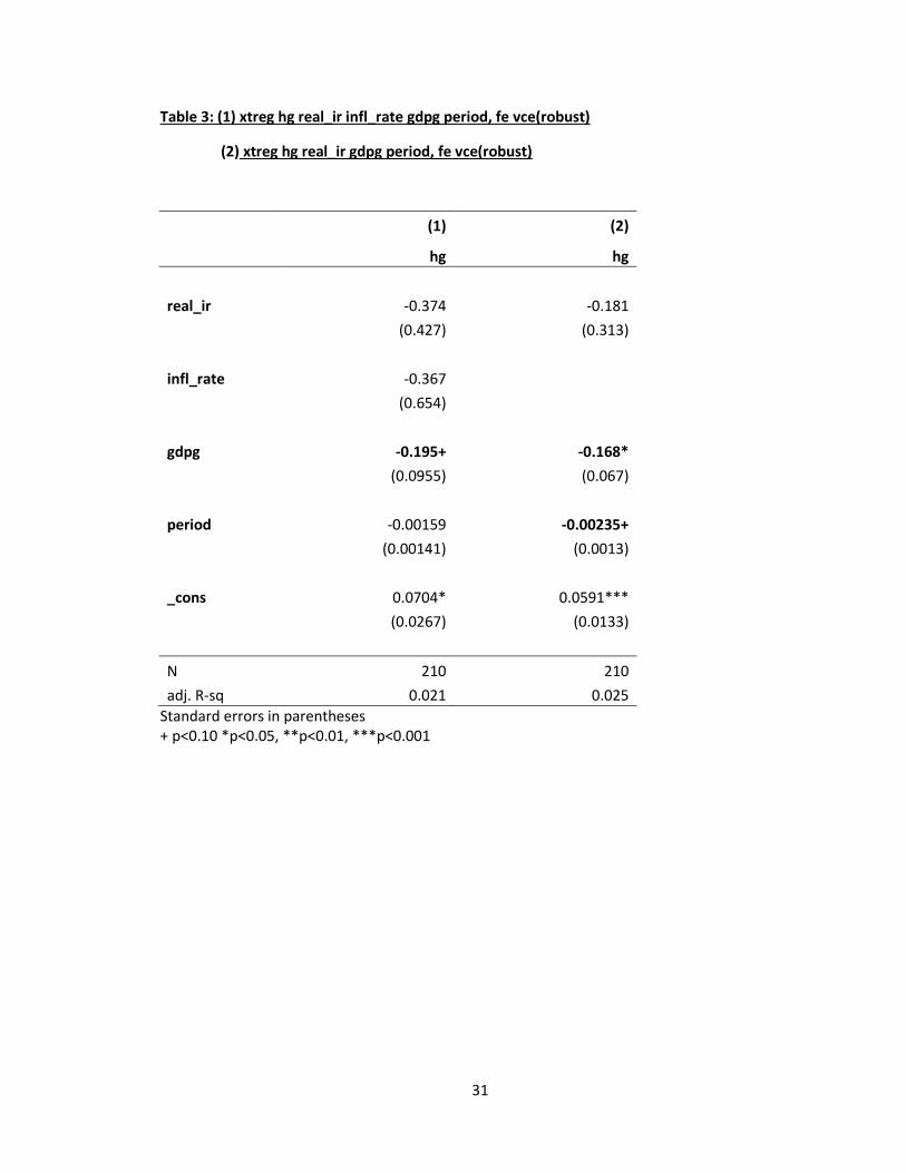
Table 3 displays the results of including a time trend along with the economic

variables. While including period along with the variables in the previous regression did

not generate statistically significant results, including the time trend with the

macroeconomic variables previously found to be significant generates a small, negative

coefficient of 0.00235 that is significant at the 10 percent level. Several variables were

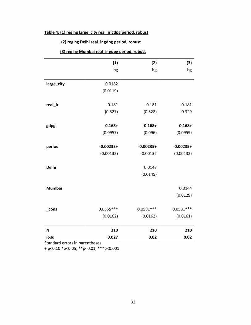
developed to draw out conclusive results on the effect of large metropolitan cities,

including Delhi, Mumbai, large_city (Delhi and Mumbai). The results in Table 4 indicate

that none of the city variables are statistically significant.

The low explanatory power and varying levels of statistical significance on the

coefficients suggest that these models do not yield clear robust interpretable insights into

22

the impacts of macroeconomic variables. Therefore, I adopt a different approach and

control for all macroeconomic movements using time period binary variables.

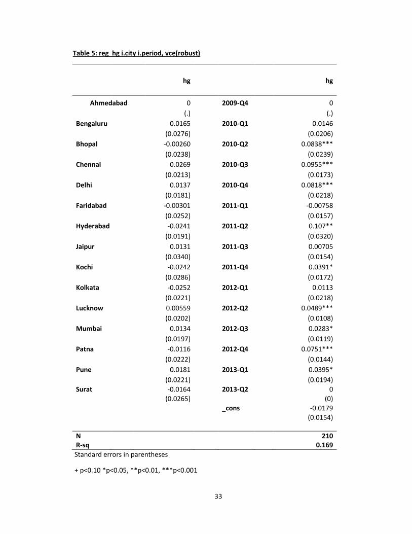
Table 5 displays the results of including binary variables to test for city-fixed

effects and time-fixed effects with hetereoscedasticity-robust standard errors. Although

none of the coefficients on city-fixed effects are statistically significant, point estimates

suggest that house price growth varies across the country with Bengaluru, Chennai,

Delhi, Mumbai, Lucknow and Pune displaying higher point estimates. It is noteworthy

that this includes four out of the six metropolitan cities in India. Several time periods

emerge as statistically significant, indicating that period binary variables were

appropriate in order to control for macroeconomic fluctuations. Additionally, the

significance of period-fixed effects can be reconciled with the insight that the

macroeconomic slowdown in FY2011-2012 had an effect on the residential real estate

market.

Next, I turn my attention towards the residuals in order to investigate alternative

models that could be appropriate. Figure 1 depicts the residuals of the time and entity-

fixed effects regression assuming heteroscedasticity-robust standard errors. The graph

suggests that the residuals are not random and correlated with adjacent observations. I

therefore test other models with auto-correlated standard errors.

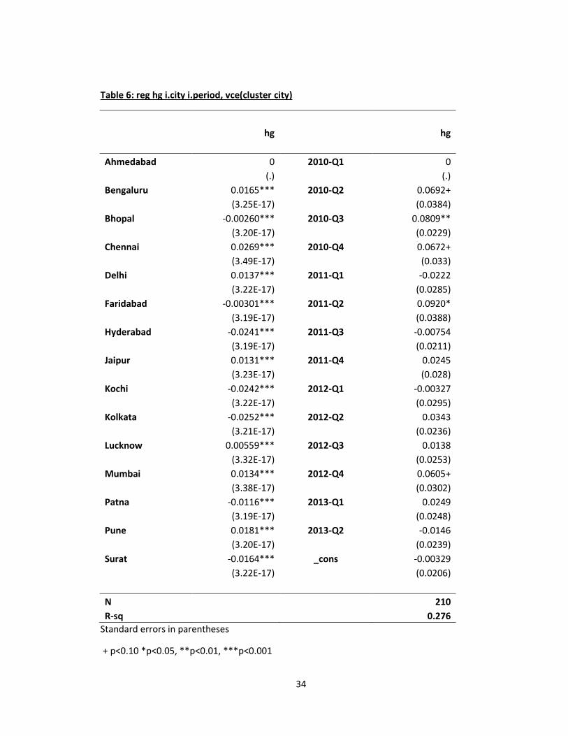
Table 6 displays the results of a clustering the standard errors on each city

assuming that they are heteroscedastic and auto-correlated. Although point estimates of

some cities (Delhi, Mumbai, Bengaluru, Chennai, Lucknow and Pune) are still higher

than the rest, the standard error on all entity fixed effects are now substantially lower,

23

making the coefficients significant at the 0.1 percent level. The implausibly low standard

error terms on each city, however, motivate me to test other models with auto-correlated

standard errors that impose more structure.

Table 7 displays the results of the city-fixed effects generated by three different

models used to impose structure on the standard errors. Model (1) imposes a common

AR1 autocorrelation structure assuming panel-level heteroscedastic errors (no cross-

sectional correlation). Model (2) imposes a panel-specific AR1 autocorrelation structure

and Model (3) imposes a panel-specific AR1 autocorrelation structure with panel-level

heteroscedastic errors. All three models suggest that Hyderabad has a negative

coefficient, statistically significant at the 10 percent level. This suggests that house price

growth has been below-normal in Hyderabad. Model (2), imposing AR1 autocorrelation

assuming no cross-sectional correlation, suggests that house prices in Kolkata display

below-normal growth (statistically significant at the 1 percent level). These models

display s of 0.295, 0.325 and 0.325 respectively, suggesting that the first model

explains ~30 percent of the variation in , and the models imposing panel-specific

AR1 autocorrelation structure explain ~33 percent.

24

IX. Conclusion

According to the available data, different models suggest that different

conclusions can be drawn about the statistical significance of macroeconomic factors

affecting the growth in house prices across India. Contrary to the literature, and

speculation about property bubbles in large metropolitan cities, my results do not provide

conclusive evidence for above-normal growth rates. One major qualification of the data,

however, is that it begins in 2009. Figure 2 shows trends in house prices during 2001-

2013 and Figure 3 shows house price growth in Delhi and Mumbai during the same

period. The graphs suggest that Delhi and Mumbai both display above-normal house

price levels, and rapid growth rates between 2005-2007 and 2011-12. Rapid increases in

growth rates during some periods justify the intuition guiding speculation about a house

price bubble. However, the evidence presented in this paper reinforces evidence

presented by Joshi (2006), suggesting that the increases in prices are not enough to draw

conclusive evidence about the existence of a bubble.

My findings suggest that a shift in the overall macroeconomic environment during

FY11-12, however, had an impact on overall growth in house prices. Due to shifts in

demographics and urbanization, residential-real estate markets are continuously evolving

across different cities within the country. A more appropriate test to evaluate the city-

specific effects of different housing markets would include population data to account for

shifts in population, construction data to account for the varying levels of real-estate

development across the country, and credit-penetration data to account for the differences

in access to housing finance across different cities. Although the findings of this thesis

are inconclusive about the existence of an asset bubble in the residential real-estate

25

market, it is imperative that future research builds on city-level models in order to

investigate the trends in house prices.

26

X. References

Moneycontrol. (2013, February 24). Retrieved November 2013, from Indian GDP estimated at

5% in FY13, lowest since FY04: http://www.moneycontrol.com/news/economy/indian-

gdp-estimated-at-5fy13-lowest-since-fy04-govt_829548.html

Anand, S. (2010, Aug 10). Indian Home Buyers Struggle with Bubble. Retrieved November 2013,

from The Wall Street Journal: Real Estate: http://profit.ndtv.com/news/your-

money/article-indias-real-estate-market-time-for-the-bubble-to-burst-371745

Bertraud, A. (2010). Land Markets, Government Interventions, and Housing Affordability.

Wolfensohn Center For Development at Brookings.

Calomiris, C. W., Longhofer, S. D., & William, M. (2012). The Housing Wealth Effect: The Crucial

Roles of Demographics, Wealth Distribution and Wealth Shares. The National Bureau of

Economic Research.

Case, K. E., & Shiller, R. J. (2004). Is There a Bubble in The Housing Market? Cowles Foundation

for Research in Economics, Yale University, 299:305.

Chadha, S. (2013, September 2). Property Bubble Bursts as Prices Crash 20 per cent in Investor-

driven Markets. Retrieved November 2013, from FirstPost Economy:

http://www.firstpost.com/economy/property-bubble-bursts-as-prices-crash-20-in-

investor-driven-markets-1077885.html

CNN IBN. (2007, 29 November). Maharashtra Assembly Repeals Urban Land Ceiling Act.

Retrieved November 2013, from IBN Live: http://ibnlive.in.com/news/maharashtra-

assembly-repeals-urban-land-ceiling-act/53283-7.html

DiPasquale, D., & Wheaton, W. C. (1996). The Urban land Market: Rents and Prices. In Urban

Economics and Real Estate Markets (pp. 34-38). New Jersey: Pearson Education.

Gandhi, S. (2012). Economics of Affordable Housing in Indian Cities: The Case of Mumbai.

Environment and Urbanization Asia.

Goodheart, C., & Hofman, B. (2007). House Prices and the Macroeconomic - Implications for

Banking and Price Stability. Chennai, India: Oxford.

IBEF. (2013, November). Real Estate Industry in India. Retrieved November 2013, from India

Brand Equity Foundation: http://www.ibef.org/industry/real-estate-india.aspx

Joshi, H. (2006). Identifying Asset Price Bubbles in the Housing Market in India - Preliminary

Evidence . Reserve Bank of India Occasional Papers.

27

Kala, A. V. (2013, Sept 2013). India Wholesale Inflation Rises. The Wall Street Journal.

KPMG. (2012). Bridging the Urban Housing Shortage in India. Mumbai: NAREDCO.

Kumar, R. (2013, November 9). India's real estate market: time for the bubble to burst? India.

Retrieved from India's real estate market: Time for the bubble to burst?:

http://profit.ndtv.com/news/your-money/article-indias-real-estate-market-time-for-

the-bubble-to-burst-371745

Lipsey, R. G., & Harbury, C. (2004). The First Principles of Economics. Oxford University Press.

Mankiw, G. N. (2011). Principles of Macroeconomics. Cengage Learning .

Ministry of Finance. (2013). Macroeconmic Framework Statement. Retrieved November 2013,

from India Budget: http://indiabudget.nic.in/ub2013-14/frbm/frbm1.pdf

Mohanty, D. (2013, May 13). Perspectives on Housing Finance in India. Retrieved November

2013, from Reserve Bank of India:

http://rbi.org.in/Scripts/BS_ViewBulletin.aspx?Id=14174

Mustafi, S. M. (2013, May 13). India's Middle Class: Growth Engine or Loose Wheel? Retrieved

November 2013, from International New York Times:

http://india.blogs.nytimes.com/2013/05/13/indias-middle-class-growth-engine-or-

loose-wheel/?_r=1

National Housing Bank. (2013, May). NHB Residex- Status, Challenges and Way Forward.

Retrieved November 2013, from

http://www.nhb.org.in/Archives/Press%20Release_Archives.php

NHB. (2012). Report on Trend and Progress of Housing in India. India: National Housing Bank.

Prem. (2012, January 30). Key Demand Drivers for the Housing Industry in India. Retrieved

November 2013, from The Finance Concept:

http://www.thefinanceconcept.com/2012/01/key-demand-drivers-for-housing-

industry.html

Rupee Manager. (2013, May 29). Overview of Housing Finance Industry in India. Retrieved

November 2013, from Rupee Manager - Personal Finance Resources:

http://rupeemanager.com/investing/loans/overview-of-housing-finance-industry-in-

india.html

Schaffer, T. C. (2013, September 23). Brookings Research. Retrieved November 2013, from

India's Sagging Economy - Strategic Consequences:

http://www.brookings.edu/research/opinions/2013/09/23-india-economy-schaffer

28

Srivastava, S. (2013, March 4). Why the Real Estate Market Could Crack in 2013. Retrieved

November 2013, from Forbes India: http://forbesindia.com/blog/business-

strategy/why-the-real-estate-market-could-crack-in-2013/

Thirani, S. (2013). The Reality of the Indian Housing Bubble. India.

29

XI. Appendix

Table 1: xtreg real_ir infl_rate gdpg, fe vce(robust)

hg

real_ir -0.679*

(0.305)

infl_rate -0.519

(0.310)

gdpg -0.212*

(0.0739)

_cons 0.0802**

(0.0244)

N 210

adj. R-sq 0.023

Standard errors in parentheses + p<0.10 *p<0.05, **p<0.01, ***p<0.001

30

Table 2: xtreg hg real_ir infl_rate gdpg period1, fe vce(robust)

hg

real_ir 0.545

(0.478)

infl_rate 0.647

(0.738)

gdpg -0.233*

(0.0923)

period1 0.0535**

(0.0171) _cons -0.0307

(0.0431)

N 210

adj. R-sq 0.060

Standard errors in parentheses + p<0.10 *p<0.05, **p<0.01, ***p<0.001

31

Table 3: (1) xtreg hg real_ir infl_rate gdpg period, fe vce(robust)

(2) xtreg hg real_ir gdpg period, fe vce(robust)

(1) (2)

hg hg

real_ir -0.374 -0.181

(0.427) (0.313)

infl_rate -0.367

(0.654)

gdpg -0.195+ -0.168*

(0.0955) (0.067)

period -0.00159 -0.00235+

(0.00141) (0.0013)

_cons 0.0704* 0.0591***

(0.0267) (0.0133)

N 210 210

adj. R-sq 0.021 0.025

Standard errors in parentheses + p<0.10 *p<0.05, **p<0.01, ***p<0.001

32

Table 4: (1) reg hg large_city real_ir gdpg period, robust

(2) reg hg Delhi real_ir gdpg period, robust

(3) reg hg Mumbai real_ir gdpg period, robust

(1) (2) (3)

hg hg hg

large_city 0.0182

(0.0119)

real_ir -0.181 -0.181 -0.181

(0.327) (0.328) -0.329

gdpg -0.168+ -0.168+ -0.168+

(0.0957) (0.096) (0.0959)

period -0.00235+ -0.00235+ -0.00235+

(0.00132) -0.00132 (0.00132)

Delhi

0.0147

(0.0145)

Mumbai

0.0144

(0.0129)

_cons 0.0555*** 0.0581*** 0.0581***

(0.0162) (0.0162) (0.0161)

N 210 210 210

R-sq 0.027 0.02 0.02

Standard errors in parentheses + p<0.10 *p<0.05, **p<0.01, ***p<0.001

33

Table 5: reg hg i.city i.period, vce(robust)

hg

hg

Ahmedabad 0

2009-Q4 0

(.)

(.)

Bengaluru 0.0165

2010-Q1 0.0146

(0.0276)

(0.0206)

Bhopal

-0.00260

2010-Q2 0.0838***

(0.0238)

(0.0239)

Chennai

0.0269

2010-Q3 0.0955***

(0.0213)

(0.0173)

Delhi

0.0137

2010-Q4 0.0818***

(0.0181)

(0.0218)

Faridabad -0.00301

2011-Q1 -0.00758

(0.0252)

(0.0157)

Hyderabad -0.0241

2011-Q2 0.107**

(0.0191)

(0.0320)

Jaipur

0.0131

2011-Q3 0.00705

(0.0340)

(0.0154)

Kochi

-0.0242

2011-Q4 0.0391*

(0.0286)

(0.0172)

Kolkata

-0.0252

2012-Q1 0.0113

(0.0221)

(0.0218)

Lucknow 0.00559 2012-Q2 0.0489***

(0.0202) (0.0108)

Mumbai 0.0134 2012-Q3 0.0283*

(0.0197) (0.0119)

Patna -0.0116 2012-Q4 0.0751***

(0.0222) (0.0144)

Pune 0.0181 2013-Q1 0.0395*

(0.0221) (0.0194)

Surat

-0.0164

2013-Q2

0

(0.0265) (0)

_cons -0.0179

(0.0154)

N 210 R-sq 0.169

Standard errors in parentheses

+ p<0.10 *p<0.05, **p<0.01, ***p<0.001

34

Table 6: reg hg i.city i.period, vce(cluster city)

hg

hg

Ahmedabad 0 2010-Q1 0

(.)

(.)

Bengaluru 0.0165*** 2010-Q2 0.0692+

(3.25E-17)

(0.0384)

Bhopal -0.00260*** 2010-Q3 0.0809**

(3.20E-17)

(0.0229)

Chennai 0.0269*** 2010-Q4 0.0672+

(3.49E-17)

(0.033)

Delhi 0.0137*** 2011-Q1 -0.0222

(3.22E-17)

(0.0285)

Faridabad -0.00301*** 2011-Q2 0.0920*

(3.19E-17)

(0.0388)

Hyderabad -0.0241*** 2011-Q3 -0.00754

(3.19E-17)

(0.0211)

Jaipur 0.0131*** 2011-Q4 0.0245

(3.23E-17)

(0.028)

Kochi -0.0242*** 2012-Q1 -0.00327

(3.22E-17)

(0.0295)

Kolkata -0.0252*** 2012-Q2 0.0343

(3.21E-17)

(0.0236)

Lucknow 0.00559*** 2012-Q3 0.0138

(3.32E-17)

(0.0253)

Mumbai 0.0134*** 2012-Q4 0.0605+

(3.38E-17)

(0.0302)

Patna -0.0116*** 2013-Q1 0.0249

(3.19E-17)

(0.0248)

Pune 0.0181*** 2013-Q2 -0.0146

(3.20E-17)

(0.0239)

Surat -0.0164*** _cons -0.00329

(3.22E-17)

(0.0206)

N 210

R-sq 0.276

Standard errors in parentheses

+ p<0.10 *p<0.05, **p<0.01, ***p<0.001

35

Table 7: (1) xtpcse hg i.city i.period, correlation (ar1) hetonly

(2) xtpcse hg i.city i.period, correlation(psar1)

(3) xtpcse hg i.city i.period, correlation(psar1) hetonly

(1) (2) (3) (1) (2) (3)

hg hg hg

hg hg hg

Ahmedabad 0 0 0 Kochi -0.0258 -0.0260 -0.0260

(.) (.) (.)

(0.0226) (0.0274) (0.0268)

Bengaluru 0.0139 0.0136 0.0136 Kolkata -0.0258 -0.0259** -0.0259

(0.0202) (0.0155) (0.0188)

(0.0166) (0.0082) (0.0170)

Bhopal -0.0042 -0.0042 -0.0042 Lucknow 0.0042 0.0045 0.0045

(0.0180) (0.0215) (0.0185)

(0.0149) (0.0094) (0.0140)

Chennai 0.0241 0.0278 0.0278 Mumbai 0.0110 0.0110 0.0110

(0.0169) (0.0272) (0.0217)

(0.0148) (0.0153) (0.0148)

Delhi 0.0131 0.0039 0.0039 Patna -0.0144 -0.0156 -0.0156

(0.0144) (0.0150) -0.0207

(0.0157) (0.0131) (0.0130)

Faridabad -0.0056 -0.0060 -0.0060 Pune 0.0159 0.0157 0.0157

(0.0185) (0.0218) (0.0175)

(0.0163) (0.0176) (0.0158)

Hyderabad -0.0262+ -0.0263+ -0.0263+ Surat -0.0175 -0.0165 -0.0165

(0.0141) (0.0153) (0.0135)

(0.0184) (0.0144) (0.0144)

Jaipur 0.0110 0.0110 0.0110 _cons -0.0015 0.0030 0.0030

(0.0254) (0.0259) (0.0243)

(0.0196) (0.0118) (0.0190)

N

210 210 210

R-sq

0.295 0.325 0.325

Standard errors in parentheses

+ p<0.10 *p<0.05, **p<0.01, ***p<0.001

36

Figure 1: Residuals of reg hg i.city i.period, vce(robust)

Figure 2: House Prices (2001-2013)

0

50

100

150

200

250

300

350

400

450

20

01

20

02

20

03

20

04

20

05

20

06

20

07

20

08

20

09

20

10

20

11

20

12

20

13

Residex (HPI)

Year

Delhi

Bangalore

Mumbai

Bhopal

Kolkata

37

Figure 3: House Price Growth (2001-2013)

-10%

-5%

0%

5%

10%

15%

20%

25%

30%

35%

2002 2003 2004 2005 2006 2007 2008 2009 2010 2011 2012 2013

Residex Growth Rate

Year

Delhi

Mumbai