The Renormalization Group (RG)

Introduction / Preliminaries Scaling limit Renormalization group transformations Summary

Handout

Hi! You can take a handout, if there is one.

The Renormalization Group (RG) Thomas Coutandin


The Renormalization Group (RG)

Thomas [email protected]

Advisors:Dr. Ch. Iniotakis, Dr. M. Matsumoto

May 07, 2007



Framework, main idea

Outline

1 Introduction / PreliminariesFramework, main ideaClassical lattice spin systems

2 Scaling limitScaled lattice system, renormalization conditionConsequences of the renormalization condition

3 Renormalization group transformationsKadanoff (RG) block spin transformationsFixed points, determination of critical exponents

4 Summary




RG as a set of symmetry transformations

Given: macroscopic physical system near a critical point.RG for our system: set of symmetry transformations (called RGtransformations).idea of these symmetry transformations: ∼ same as in Atomicphysics (for example). Differences:

The whole system will not be simply invariant under a RGtransformation.It is not so easy to find a RG.The RG is not a group.

carrying out a symmetry transformation means not the same assolving a particular model




Our Job

Our job: Find a RG for our system (there may be many).The idea: Study the behavior of our system under a change ofscale.




What do we get from RG theory?

We get a connection to QFT.The critical exponents appear as symmetry properties of theRG transformations:

As a direct consequence of having found a RG for our system weget the scaling relations corresponding to our system.But not only the scaling relations: there is a way to calculatecritical exponents.




Framework

Theory of Phase TransitionsTheory of Critical PhenomenaClassical statistical mechanicsLattice spin systems




Bibliography

This talk is mainly based on a paper of J. Fröhlich and T. Spencer, see[1] in Bibliography (Handout).




Outline




4 Summary




Outline




4 Summary




Outline




4 Summary




Outline




4 Summary



Classical lattice spin systems

Outline




4 Summary




Justifications

In the following we will only consider the simplest, classical spinsystems, namely lattice ones. For the following treatment we shouldjustify the following:

the use of classical spin systems.considering infinitely large lattice systems.considering only the (hyper-) cubic lattice.




1. Lattice

The lattice is chosen to be the simple (hyper-) cubic lattice, Zd. Witheach lattice site j ∈ Zd associated is a classical spin

ϕ(j) ∈ RN(j) � R

N ,

where N is the dimension of spin space (for all lattice sites the same).For Λ ⊂ Zd define the spin configuration on Λ to be

ϕΛ := {ϕ(j) : j ∈ Λ} ,

which is contained in the space of all spin configurations on Λ,

KΛ :=∏j∈Λ

RN(j) .

We set K∞ ≡ KZd .The Renormalization Group (RG) Thomas Coutandin



2. Spin

The further characterization of the spin is given by the a prioridistribution of the spin. For an arbitrary spin ϕ(j), j ∈ Zd , it is givenby a probability measure, dλ(ϕ(j)), on the Borel sets of RN . Note that itis defined to be the same for all sites j ∈ Zd .Now let Λ ⊂ Zd be a finite subset of the lattice. Then the a prioridistribution of a spin configuration on Λ is given by∏

j∈Λ

dλ(ϕ(j)) ,

which is a probability measure on KΛ.




3. Energy

For a finite sublattice Λ we define the Hamilton function:

HΛ : KΛ → R , ϕΛ 7→ HΛ(ϕΛ)

Assumption: HΛ(ϕΛ) is continuous on KΛ.β ≡ (kT )−1 ≥ 0: inverse temperature




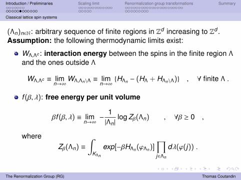
(Λn)n∈N: arbitrary sequence of finite regions in Zd increasing to Zd .Assumption: the following thermodynamic limits exist:

WΛ,Λc : interaction energy between the spins in the finite region Λand the ones outside Λ

WΛ,Λc ≡ limn→∞

WΛ,Λn\Λ ≡ limn→∞

{HΛn − (HΛ + HΛn\Λ)} , ∀ finite Λ .

f (β, λ): free energy per unit volume

βf (β, λ) ≡ limn→∞

−1|Λn|

log Zβ(Λn) , ∀β ≥ 0 ,

whereZβ(Λn) ≡

∫KΛn

exp[−βHΛn(ϕΛn)]∏j∈Λn

dλ(ϕ(j)) .




4. Equilibrium state

An equilibrium state at inverse temperature β of the infinite latticespin system is given by a probability measure, dµβ,λ(ϕ), on K∞ with thefollowing defining property:For every bounded measurable function A on KΛ, where Λ is anarbitrary finite sublattice, the following holds:

〈A〉β,λ ≡∫K∞

A(ϕΛ)dµβ,λ(ϕ)

=

∫KΛc

dρ(ϕΛc )

∫KΛ

e−β(WΛ,Λc (ϕ) + HΛ(ϕΛ))A(ϕΛ)∏j∈Λ

dλ(ϕ(j)) ,

where dρ(ϕΛc ) is a finite measure on KΛc . These are the so calledDobrushin-Lanford-Ruelle equations.




Simplification

For simplicity: N = 1 (N: dimension of spin space)




Correlation functions

⟨ϕ(x1) · · · ϕ(xn)

⟩β ≡

⟨ n∏k=1

ϕ(xk )

⟩β

=

∫K∞

n∏k=1

ϕ(xk ) dµβ(ϕ) . (1)




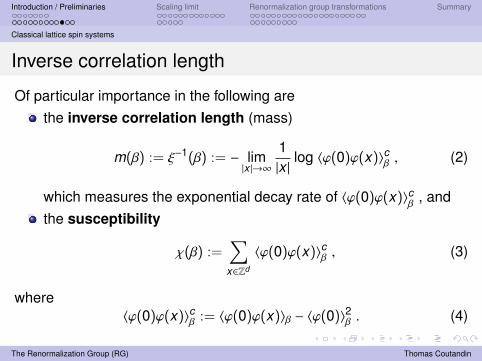
Inverse correlation length

Of particular importance in the following arethe inverse correlation length (mass)

m(β) := ξ−1(β) := − lim|x |→∞

1|x |

log 〈ϕ(0)ϕ(x)〉cβ , (2)

which measures the exponential decay rate of 〈ϕ(0)ϕ(x)〉cβ , andthe susceptibility

χ(β) :=∑x∈Zd

〈ϕ(0)ϕ(x)〉cβ , (3)

where〈ϕ(0)ϕ(x)〉cβ := 〈ϕ(0)ϕ(x)〉β − 〈ϕ(0)〉2β . (4)




Critical point

In the following we will only consider phase transitions at a criticalpoint. β = βc is defined to be a critical point if

m(β)↘ 0 , as β↗ βc , or β↘ βc . (5)




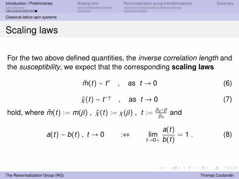
Scaling laws

For the two above defined quantities, the inverse correlation length andthe susceptibility, we expect that the corresponding scaling laws

m̃(t) ∼ tν , as t → 0 (6)

χ̃(t) ∼ t−γ , as t → 0 (7)

hold, where m̃(t) := m(β) , χ̃(t) := χ(β) , t := βc−ββc

and

a(t) ∼ b(t) , t → 0 :⇔ limt→0+

a(t)b(t)

= 1 . (8)



Scaled lattice system, renormalization condition

Outline




4 Summary




For the following we consider the case in which

β < βc .




Assumptions (equilibrium state, inv. correl. length):

The equilibrium state dµβ(ϕ) is invariant under lattice translations ,i.e.

∀x ∈ Zd : dµβ(ϕx) = dµβ(ϕ) ,

whereϕx(j) = ϕ(j + x) , x , j ∈ Zd .

For β < βc , the equilibrium state dµβ is extremal invariant, i.e.ergodic under the action of lattice translations.the inverse correlation length, m(β), is positive and continuous inβ, with

m(β)↘ 0 , as β↗ βc . (9)




Large scale behavior of the correlation functions

Due to the divergence of the correlation length, ξ ≡ m(β)−1, at a criticalpoint we are interested in the large scale behavior of the correlationfunctions

〈ϕ(z1) · · ·ϕ(zn)〉β , β near to βc (zi ∈ Zd ,1 ≤ i ≤ n) ; (10)

more precisely we are interested in the long distance limit of (10), inwhich

|zi − zj | → ∞ , whenever i , j . (11)




Scale transformation

In order to realize such a limit we consider a scale transformation

Zd → Zdϑ−1 := {y ∈ Rd : ϑy ∈ Zd } , z 7→ ϑ−1z (12)

where ϑ ∈ [1,∞[ is called a scale parameter. Next, for given pointsxk ∈ Z

d ⊂ Rd , 1 ≤ k ≤ n, we choose for every ϑ ∈ [1,∞[ functionsϑ 7→ xi(ϑ) ∈ Z

dϑ−1 ⊂ R

d , 1 ≤ i ≤ n, in such a way that

xi(ϑ) = xi + O(ϑ−1) , (ϑ→ ∞) . (13)

In particular we get

|xi(ϑ) − xj(ϑ)| = |xi − xj |+ O(ϑ−1) , (ϑ→ ∞) . (14)

Then in the scaling limit, in which

ϑ→ ∞ , (15)

the corresponding points zi = zi(ϑ) := ϑxi(ϑ) ∈ Zd satisfy (11).




General strategy, RG transformationconstruct from our real lattice system in some way, including theabove scale transformation with scale parameter ϑ, an ”effective”one.First step: construction of a scaled lattice system, ”naturally”determined by the scale transformation (12).Second step: construction of an effective lattice system of Zd

RG transformation: transformation mapping the original state ofour real system to the effective stateCrucial: construction of the RG transformation itsself, i.e.transf. actually realized as a symmetry transformation.Note: (scaled) ”effective” lattice system only a construction;motivation: extract the effective large scale behavior of thecorrelation functions from our physical lattice system Zd .




Construction of a scaled lattice system

Define the scaled spin, ϕ(ϑ), on Zdϑ−1 as

ϕ(ϑ) : Zdϑ−1 → R

d , x 7→ ϕ(ϑ)(x) := α(ϑ) ϕ(ϑx) , (16)

where α(ϑ) is a positive rescale factor.scaled parameters (w.r.t. Zd

ϑ−1) corresponding to just these(thermodynamic) parameters, which determine the equilibriumstate of our real lattice system Zd . One such parameter is theinverse temperature β.





Want the RG transformation be realized as a symmetrytransformation.Therefore we require, due to (2), the ”scaled inversetemperature”, β(ϑ), to satisfy

β(ϑ) < βc , ∀ϑ ∈ [1,∞[ . (17)





Intuitively expecting but also motivated by the fact that (free) energyhas scale dimension 0 we set (with obvious notation):

H(ϑ)

ϑ−1Λ(ϕ(ϑ)) := HΛ(ϕ) , dλ(ϑ)

(ϕ(ϑ)(ϑ−1j)

):= dλ(ϕ(j)) , j ∈ Zd .

(18)





Define the scaled equilibrium state of Zdϑ−1 , denoted by dµ(ϑ)

β(ϑ),

to be the probability measure which solves theDLR-equations, wherein all expressions are replaced by theirscaled counterparts.

Corresponding (expectation value) functional: 〈·〉(ϑ)β(ϑ)

.

Note that due to (18) dµ(ϑ)β(ϑ)

differs from dµβ only in respect thereofthat the scaled parameters have to be brought in, instead of theunscaled ones. Therefore

dµ(ϑ)β(ϑ)

(ϕ(ϑ)) = dµβ(ϑ)(ϕ) . (19)





Now we can define the scaled correlations for points yi ∈ Zdϑ−1

(1 ≤ i ≤ n, ϑ ∈ [1,∞[) :

Gϑ(y1, . . . , yn) :=⟨ϕ(ϑ)(y1) · · ·ϕ

(ϑ)(yn)⟩(ϑ)β(ϑ)

(20)

(16)=

(19)α(ϑ)n ⟨

ϕ(ϑy1) · · ·ϕ(ϑyn)⟩β(ϑ) (21)

(also called rescaled correlation function).




Renormalization condition

This finally enables us to state the renormalization condition:For x1, . . . , xn ∈ Z

d :

0 < |xi − xj | < ∞ , n ≥ 2⇒ 0 < G∗(x1, . . . , xn) := lim

ϑ→∞Gϑ(x1(ϑ), . . . , xn(ϑ)) < ∞ (22)

G∗(x1, . . . , xn) is called limiting correlation function.




General renormalization condition

The above condition (22) is only the renormalization condition fora RG transformation which ends up with the ”scaled” state dµβ(ϑ)(see (19)) as effective state of Zd .In general, where the RG transformation ends up with just anyeffective state of Zd , the general renormalization condition isobtained by considering the scaling limit of the correlationfunction with respect to the effective state.



Consequences of the renormalization condition

Outline




4 Summary




Summary: Consequences of the renormalizationcondition

The renormalization condition yields a connection to QFT.The renormalization condition implies non-trivial scaling relationsbetween critical exponents.(determination of critical exponents) An explicit construction ofthe renormalization condition determines, in principle, the criticalexponents ν, γ and η.




A second ”renormalization condition”

In order to get a scaling relation between the critical exponents η, νand γ, it suffices to show a second ”renormalization condition” (inaddition to (22)):

ϑm(β(ϑ))→ m∗ > 0 , as ϑ→ ∞ . (23)




Consequences of the renormalization condition(s)

Scaled inverse temperature determined by ν :

βc − β(ϑ) ∼ ϑ− 1ν , ϑ→ ∞ . (24)

Scaling relation:(2 − η)ν − γ = 0 (25)




Determination of critical exponents

An explicit construction of the renormalization condition, i.e. havingfound a choice for the functions α(ϑ) and β(ϑ), determines, in principle,the critical exponents ν, γ and η:α(ϑ) determines η via (definition η):

α(ϑ)2 ∼ ϑd−2+η , ϑ→ ∞ . (26)

β(ϑ) determines ν by (24), andγ is then obtained via the scaling relation (25).



Renormalization group transformations

Here we only study the static (time-averaged) case but thereexists a RG theory for dynamics as well.The ultimate ambition of RG theory is the construction of anon-trivial limiting correlation function, i.e. theaccomplishment of a renormalization condition.a RG transformation is a combination of a scale transformationand some coarse graining process, leading finally to an effectivestate.

Typical example of a RG transformations: RG block spintransformations.



Kadanoff (RG) block spin transformations

Outline




4 Summary




RG block spin transformation

A RG block spin transformation consists of two transformations:a scale transformation anda block spin transformation.

The latter one is the reason why this kind of RG transformation isreferred to as RG block spin transformation. As stated above, a scaletransformation is somehow incorporated in every RG transformation.




Scale transformation

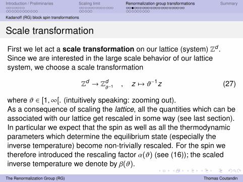
First we let act a scale transformation on our lattice (system) Zd .Since we are interested in the large scale behavior of our latticesystem, we choose a scale transformation

Zd → Zdϑ−1 , z 7→ ϑ−1z (27)

where ϑ ∈ [1,∞[. (intuitively speaking: zooming out).As a consequence of scaling the lattice, all the quantities which can beassociated with our lattice get rescaled in some way (see last section).In particular we expect that the spin as well as all the thermodynamicparameters which determine the equilibrium state (especially theinverse temperature) become non-trivially rescaled. For the spin wetherefore introduced the rescaling factor α(ϑ) (see (16)); the scaledinverse temperature we denote by β(ϑ).




block spin transformation

Second we will do a block spin transformation, which is a (linear)transformation in spin (configuration) space KZd .The construction is described below.




Block size

Characteristic to any block spin transformation is a number

L ∈ N : L > 1 , (28)

called block size. For the following we fix it.




Main idea

The main idea is now to ”divide” the scaled lattice Zdϑ−1 , ϑ ∈ [1,∞[ , into

(hyper-) cubic blocks with side length ε := ϑ−1L, then to take anaverage of all the spins contained in a block – this average one mightcall block spin – and identifying each block with a site in Zd ; with thissite is then associated the block spin.




Main idea - continued

Depending on how big ϑ was chosen in the scale transformation onemight want to average over a bigger block with side length ε := ϑ−1Lm.The question which then automatically arises is: How big do we wantto have ε ? Since we want to identify each block with a site in Zd , agood answer is certainly ε ≈ 1. Therefore define

m ≡ m(ϑ) := min {j ∈ N : ϑ ≤ Lj } (29)

and set the scaled ”block” size to be

ε := ϑ−1Lm(ϑ) . (30)




Hence1 ≤ ε < L . (31)

Note that due to (31)

ϑ→ ∞ ⇔ m → ∞ . (32)

When we use the latter as scaling limit we write ϑm instead of ϑ inorder to remind of (32).




Construction of an effective lattice (system) Zd

”Effective”: in the sense that we extract only relevant informationfrom Zd

ϑ−1 .

Divide the lattice Zdϑ−1 into ε-blocks (blocks with side length ε) so

that: ε-blocks centered in exactly these points which are containedin C := {y ∈ Zd

ϑ−1 | ∃x ∈ Zd : y = εx}.

Realizing that Zd is naturally contained in ZdL−m we do the following

”identification map”

Zdϑ−1 → Z

dL−m , y 7→ ε−1y , (33)

which maps any ε-block centered in y := εx ∈ C ⊂ Zdϑ−1 , x ∈ Zd , to

an 1-block centered in x ∈ Zd ⊂ ZdL−m .




Construction of an effective lattice (system) Zd

Associate with each site x ∈ Zd ⊂ ZdL−m a block spin (r (ϑ)ϕ)(x),

which is the average of all spins that are ”contained” in the ε-blockcentered in εx ∈ Zd

ϑ−1 .It follows the ultimate block spin transformation, a lineartransformation in spin configuration space KZd , transforming themeasure µβ(ϑ) into a measure R(ϑ)µβ(ϑ), which means intuitivelyestablishing the block spin as a ”real” spin on Zd .To what extent the measure R(ϑ)µβ(ϑ) really describes an(”effective”) equilibrium state on Zd will then be discussed.

After having constructed the block spin: ”forget” the points contained inZd

L−m \ Zd . What we regard as relevant information has been absorbed

into the block spin.




Now we want to introduce the notions ofblock spin andblock correlation function




Block spin

Now define the block spin, (r (ϑ)ϕ)(x), at site x ∈ Zd to be

(r (ϑ)ϕ)(x) :=1

(Lm)d

∑y ∈ Zd

ϑ−1

‖ε−1y−x‖∞≤ 12

ϕϑ(y) (34a)

(16)=

1(Lm)d

∑y ∈ Zd

ϑ−1

‖ε−1y−x‖∞≤ 12

α(ϑ) ϕ(ϑy) . (34b)

The average is taken in dividing by (Lm)d = (ϑε)d instead of εd . We dothis because we get then the right average in the trivial case, whereϑ = 1.




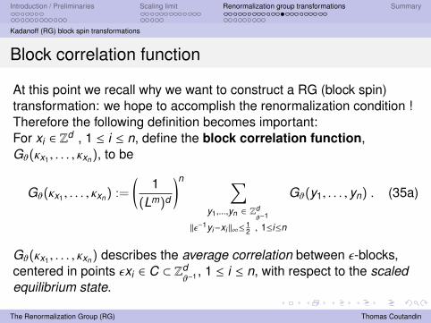
Block correlation function

At this point we recall why we want to construct a RG (block spin)transformation: we hope to accomplish the renormalization condition !Therefore the following definition becomes important:For xi ∈ Z

d , 1 ≤ i ≤ n, define the block correlation function,Gϑ(κx1 , . . . , κxn), to be

Gϑ(κx1 , . . . , κxn) :=

(1

(Lm)d

)n ∑y1,...,yn ∈ Z

dϑ−1

‖ε−1yi−xi ‖∞≤12 , 1≤i≤n

Gϑ(y1, . . . , yn) . (35a)

Gϑ(κx1 , . . . , κxn) describes the average correlation between ε-blocks,centered in points εxi ∈ C ⊂ Zd

ϑ−1 , 1 ≤ i ≤ n, with respect to the scaledequilibrium state.




Then:

Gϑ(κx1 , . . . , κxn)(35a)=

(1

(Lm)d

)n ∑y1,...,yn ∈ Z

dϑ−1

‖ε−1yi−xi ‖∞≤12 , 1≤i≤n

Gϑ(y1, . . . , yn)

(20)=

(1

(Lm)d

)n ∑y1,...,yn ∈ Z

dϑ−1

‖ε−1yi−xi ‖∞≤12 , 1≤i≤n

α(ϑ)n ⟨ϕ(ϑy1) · · ·ϕ(ϑyn)

⟩β(ϑ)

(34b)=

⟨(r (ϑ)ϕ)(x1) · · · (r (ϑ)ϕ)(xn)

⟩β(ϑ). (36)

Intuitively (37) says that the average correlation between the spinscontained in ε-blocks, centered in points εxi ∈ C ⊂ Zd

ϑ−1 , xi ∈ Zd , with

respect to the scaled equilibrium state is just the correlation betweenthe block spins in xi ∈ Z

d , 1 ≤ i ≤ n, with respect to the state dµβ(ϑ) onZd .




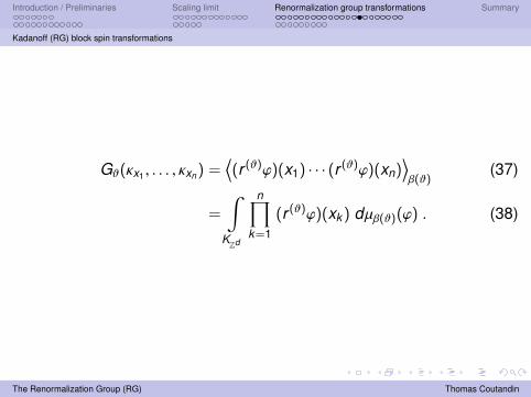
Gϑ(κx1 , . . . , κxn) =⟨(r (ϑ)ϕ)(x1) · · · (r (ϑ)ϕ)(xn)

⟩β(ϑ)

(37)

=

∫KZd

n∏k=1

(r (ϑ)ϕ)(xk ) dµβ(ϑ)(ϕ) . (38)




Block spin transformation

Since dµβ(ϑ) is a translation-invariant (finite) probability measure onKZd there is a unique (finite) probability measure R(ϑ)µβ(ϑ) on KZd suchthat:∫

KZd

n∏k=1

(r (ϑ)ϕ)(xk ) dµβ(ϑ)(ϕ) =

∫KZd

n∏k=1

ϕ(xk ) d(R(ϑ)µβ(ϑ))(ϕ) , (39)

for all xi ∈ Zd , (1 ≤ i ≤ n), and n ∈ N \ {0}.




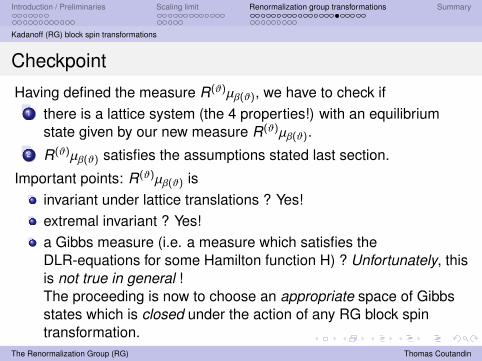
Checkpoint

Having defined the measure R(ϑ)µβ(ϑ), we have to check if1 there is a lattice system (the 4 properties!) with an equilibrium

state given by our new measure R(ϑ)µβ(ϑ).2 R(ϑ)µβ(ϑ) satisfies the assumptions stated last section.

Important points: R(ϑ)µβ(ϑ) isinvariant under lattice translations ? Yes!extremal invariant ? Yes!a Gibbs measure (i.e. a measure which satisfies theDLR-equations for some Hamilton function H) ? Unfortunately, thisis not true in general !The proceeding is now to choose an appropriate space of Gibbsstates which is closed under the action of any RG block spintransformation.




Renormalization condition

Finally from (38) and (39) we get

G∗(κx1 , . . . , κxn) := limϑ→∞

Gϑ(κx1 , . . . , κxn)

= limϑ→∞

∫KZd

n∏k=1

ϕ(xk ) d(R(ϑ)µβ(ϑ))(ϕ) , (40)

provided the limit exists.




Choosing the rescale factor for the spin: α(ϑ)

In order to arrive at an interesting concept we now suppose that α(ϑ) is”proportional” to some power of ϑ,

α(ϑ)2 ∼ ϑd−2+η , ϑ→ ∞ , (41)

for some η (this is the definition of η).




Iteration: splitting R(ϑ)

”Small” block spin:

(rϕ)(x) := L(η−d−2)/2∑

z ∈ Zd

‖L−1z−x‖∞≤ 12

ϕ(z) . (42)

Connection: block spin←→ ”Small” block spin

(r (ϑ)ϕ)(x) = α(ε−1) (rm(ϑ)ϕ)(x) . (43)




Analogous to (39) define Rµβ(ϑ) to be the unique measure on KZd suchthat: ∫

KZd

n∏k=1

(rϕ)(xk ) dµβ(ϑ)(ϕ) =

∫KZd

n∏k=1

ϕ(xk ) d(Rµβ(ϑ))(ϕ) , (44)

for all xi ∈ Zd , (1 ≤ i ≤ n), and n ∈ N \ {0}. Then∫

KZd

n∏k=1

(r (ϑ)ϕ)(xk ) dµβ(ϑ)(ϕ) =

∫KZd

n∏k=1

ϕ(xk ) d(Rm(ϑ)µβ(ϑ))(α(ε)ϕ) .

(45)Due to uniqueness we get

d(R(ϑ)µβ(ϑ))(ϕ) = d(Rm(ϑ)µβ(ϑ))(α(ε)ϕ) . (46)




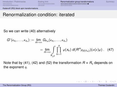
Renormalization condition: iterated

So we can write (40) alternatively

G∗(κx1 , . . . , κxn) := limm→∞

Gϑm(κx1 , . . . , κxn)

= limm→∞

∫KZd

n∏k=1

ϕ(xk ) d(Rmµβ(ϑm))(α(ε)ϕ) . (47)

Note that by (41), (42) and (52) the transformation R ≡ Rη depends onthe exponent η.



Fixed points, determination of critical exponents

Outline




4 Summary




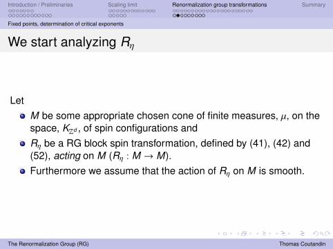
We start analyzing Rη

LetM be some appropriate chosen cone of finite measures, µ, on thespace, KZd , of spin configurations andRη be a RG block spin transformation, defined by (41), (42) and(52), acting on M (Rη : M → M).Furthermore we assume that the action of Rη on M is smooth.




Fixed point

Then, a fixed point of Rη is a point µ∗ ∈ M which is invariant under theaction of Rη, i.e.

Rη µ∗ = µ∗ . (48)

Obviously, if the scaling limit of a state dµ,

dµ∗(ϕ) := d( limm→∞

Rmµ)(ϕ) , (49)

exists, then dµ∗ is a fixed point.




General strategy

Assume:we already know η ←→ α(ϑ) (corresponding to a specificclass of spin systems)the existence of a fixed point of Rη.

Strategy: find all fixed points of RηAssume: State of a specific spin system will be driven to one of thosefixed points.

Found a fixed point? −→ calculate the critical exponents,corresponding to this fixed point (Coming soon.)Idea: study how Rη behaves in the vicinity of a fixed point −→

linearization of Rη at µ∗.ν −→ β(ϑ) −→ RG transformation is constructed




Stable, unstable manifolds

Now we choose a fixed point, µ∗, of Rη. We defineMf .p. ≡ Mf .p.(Rη, µ∗) to be the manifold of all fixed points of Rηpassing through µ∗.

Under suitable conditions on M and Rη one can decompose M in thevicinity of µ∗ into an stable manifold, Ms(µ

∗), and an unstablemanifold, Mu(µ∗), defined as follows:

states on Ms(µ∗) are driven towards µ∗ and

states on Mu(µ∗) are driven away from µ∗.




”Relevant perturbations”

We are interested in the tangent spaces of these three manifolds at thepoint µ∗:

C denotes the tangent space to Mf .p.(Rη, µ∗).The tangent space, I, to Ms(µ

∗), called space of ”irrelevantpertubations”, is the vector space spanned by eigenvectors ofDRη(µ∗) corresponding to eigenvalues of modulus < 1.The tangent space, R, to Mu(µ∗), called space of ”relevantpertubations”, is the vector space spanned by eigenvectors ofDRη(µ∗) corresponding to eigenvalues of modulus > 1.

And then there isthe tangent space,M, at µ∗, called space of ”marginalperturbations”, which is the vector space spanned by eigenvectorsof DRη(µ∗) corresponding to eigenvalues of modulus 1.




Determination of the critical exponents ν and γ

The critical exponents ν and γ are determined by the spectrum ofDRη(µ∗), more precisely by the relevant eigenvalues (which havemodulus > 1) of DRη(µ∗).




Assumption tangent space

Assumption: The tangent space at µ∗ splits intoa one-dimensional space of relevant perturbations anda co-dimension-one space of irrelevant perturbations,

which means in particular that there are no further marginalperturbations. Assuming smoothness properties we get the startingpoint for the determination of the critical exponents:For some neighborhood of µ∗ there exist a one-dimensionalunstable and a co-dimension-one stable manifold passingthrough µ∗.




The critical exponents

space of relevant perturbations: 1-D=⇒ ∃ unique simple relevant eigenvalue λWe get

ν =log(L)

log(λ)(50)

Independent of L !Via scaling relation we get the critical exponent γ.



Summary

Starting point: At a critical point, the correlation length ξ ≡ m−1

diverges.look at large scale behavior of correlation functions.scale transformation −→ scaled lattice system

This leads to the construction of a RG transformation ending up witha renormalization condition: non-trivial existence of a limitingcorrelation function. Consequences:

Scaling relations between critical exponentsDetermination of critical exponentsConnection to QFT



Crucial: construction of a RG BS transformation

Choice of α(ϑ) ←→ η

”Small” block spin:

(rϕ)(x) := L(η−d−2)/2∑

z ∈ Zd

‖L−1z−x‖∞≤ 12

ϕ(z) . (51)

”Small” block spin transformation:∫KZd

n∏k=1

(rϕ)(xk ) dµβ(ϑ)(ϕ) =

∫KZd

n∏k=1

ϕ(xk ) d(Rµβ(ϑ))(ϕ) . (52)

for all xi ∈ Zd , (1 ≤ i ≤ n), and n ∈ N \ {0}.



Crucial: construction of a RG BS transformation

Find fixed point of R ≡ Rη .Determination of ν by the relevant eigenvalues of the linearizationof the RG transformation at a fixed point.

ν =log(L)

log(λ)(53)

ν −→ β(ϑ) −→ S(ϑ) , where

S(ϑ)µβ := µβ(ϑ) (54)

The RG BS transformation, R(ϑ)S(ϑ) , is constructed.



Connection to QFT

The limiting correlation functions of a classical lattice spinsystem may be the Euclidean Green’s functions of a relativisticquantum field theory satisfying the Wightman axioms (W0)-(W5),i.e.

G∗(x1, . . . , xn) ≡ Sn(x1, . . . , xn) (55)


Documents

The Renormalization Group (RG)