1

The Remarkable Multidimensionality in the

Cross-Section of Expected U.S. Stock Returns

Jeremiah Green John R. M. Hand* X. Frank Zhang

Penn State University UNC Chapel Hill Yale University

jrg28@psu.edu hand@unc.edu frank.zhang@yale.edu

Abstract

20+ years after Fama & French (1992), we re-measure the dimensionality of the cross-section of

expected U.S. monthly stock returns in light of the large number of return predictive signals (RPS)

that have been identified by business academics over the past 40 years. Using 100 readily

programmed RPS, we find that a remarkable 24 are multidimensionally priced as defined by their

mean coefficients having an absolute t-statistic 3.0 in Fama-MacBeth regressions where all RPS

are simultaneously projected onto 1-month ahead returns during 1980-2012. We confirm the high

degree of dimensionality in returns using factor analysis of RPS, factor analysis of long/short RPS

hedge returns, LASSO regression, regressions of portfolio returns on RPS factor returns, and out-of-

sample RPS hedge portfolio returns. We put forward a new empirically determined 10-RPS model

of expected returns for consideration by researchers and practitioners. We also discuss other

implications of our findings, chief of which is the need for research that explains why stock returns

are so multidimensional and why the most empirically important RPS are priced the way they are.

This version: April 2, 2014

* Corresponding author. Our paper has greatly benefitted from the comments of Jeff Abarbanell, Sanjeev

Bhojraj, Matt Bloomfield, John Cochrane, Oleg Grudin, Bruce Jacobs, Bryan Kelly, Juhani Linnainmaa,

Ed Maydew, Scott Richardson, Jacob Sagi, Eric Yeung, and workshop participants at the University of

Chicago, Cornell University, UNC Chapel Hill, the Fall 2013 Conference of the Society of Quantitative

Analysts, and the Fall 2013 Chicago Quantitative Alliance Conference. The SAS programs we use to

create our RPS data and execute most of our statistical analyses will be made publicly available on 7/1/14.

2

1. Introduction

In their seminal study, Fama and French (1992, FF92) measured the dimensionality of the

cross-section of expected monthly U.S. stock returns. After jointly evaluating the roles of beta, firm

size, book-to-market, earnings-to-price and leverage, they observed that while beta was not

associated with expected returns, firm size and book-to-market were, and in a manner that absorbed

the unidimensional explanatory power of earnings-to-price and leverage. FF92 concluded that over

the period 1963-1990, the cross-section of monthly U.S. stock returns was two-dimensional, but that

neither dimension was consistent with the CAPM. A third dimension in the form of 12-month return

momentum (Jegadeesh, 1990; Jegadeesh and Titman, 1993) was added in Fama and French (1996)

and Carhart (1997) to create what has for two decades been seen in academia and much investment

practice as the default and conventional three-dimensional set of firm-specific risks that explain

equity returns (Royal Swedish Academy of Sciences, 2013, p.43).

The chief goal of our paper is to re-measure the dimensionality of the cross-section of

expected U.S. stock returns in light of the 330+ firm-level return predictive signals (RPS) that have

been identified by business academics since 1970 (Green, Hand and Zhang, 2013; Harvey, Liu and

Zhu, 2013). By updating the empirical dimensionality of the cross-section of expected monthly

returns, our study carries out Cochrane‘s 2010 AFA Presidential Address in which he issues a

‗multidimensional challenge‘ and calls for Fama and French‘s ‗anomaly digestion exercise‘ to be

repeated, and executes Goyal‘s (2012) recent call for researchers to ‗synthesize the huge amount of

collected [RPS] evidence.‘ In doing so, we seek to answer two of the main questions posed by

Cochrane namely: ―Which characteristics really provide independent information about mean

returns?‖ and ―Which characteristics are subsumed by other RPS?‖ (Cochrane 2011, p.1060),

Our main finding is that over the period 1980-2012, the dimensionality of monthly U.S. stock

returns is almost 10 times that originally estimated by FF92. Specifically, we document that 24 out

of 100 previously documented RPS are reliably multidimensionally priced, as defined by their mean

coefficient estimate having an absolute t-statistic 3.0 in Fama-MacBeth regressions where all 100

RPS are simultaneously projected onto 1-month ahead returns.1,2 The remarkable degree of

1 While we use the present tense when describing the dimensionality of returns, we recognize that our analysis is

historical and so may not describe the dimensionality of returns going forward beyond our sample period. 2 We use 3.0 as the absolute t-statistic cutoff for inferring statistical significance based on the insights of Harvey,

Liu, and Zhu (HLZ, 2013). HLZ seek to answer the related but different question of whether the documented hedge

returns to unidimensioned RPS are real or whether they are statistical artifacts stemming from multiple testing of the

3

multidimensionality we observe in part reflects the fact that the mean absolute cross-correlation

among RPS as measured in scaled decile ranks is small, just 0.08. We confirm the high degree of

dimensionality in several ways, including through factor analysis of RPS, factor analysis of

long/short RPS hedge returns, LASSO regression, out-of-sample RPS hedge portfolio returns, and

regressions of portfolio returns on RPS factor-mimicking-portfolio returns.

A second goal of our study is to describe key economic aspects of RPS pricing when viewed

from a multidimensional perspective. Among a number of results, we observe that although firm

size, book-to-market, and 12-month momentum in certain instances provide a reasonable

representation of expected returns, the restricted three-dimensional model misses economically

important aspects of the cross-section of returns. For example, we show that only infrequently do

firm size, book-to-market, and 12-month momentum have multidimensioned t-statistics that are large

enough to place in the top ten t-statistics of all multidimensioned RPS, and when used alone as a set

of characteristics, firm size, book-to-market, and 12-month momentum miss a large portion of the

variation that is explained by the expanded set of 24 multidimensionally priced RPS. We also

observe that while large-cap firms have far fewer multidimensionally priced RPS than do mid-cap or

small-cap firms, their RPS explain three times as much cross-sectional variation in returns, and that

the hedge returns earned by multidimensioned RPS are on average one half to two thirds smaller than

those earned by unidimensioned RPS and their t-statistics are 50% smaller. Additionally, and of

potential importance to practitioners, we document that the out-of-sample standard 2X gross levered

hedge portfolio of the full set of RPS that we study yields a monthly return of 2.7% with an

annualized Sharpe ratio of 2.6. We unpack these findings in more detail in sections 4-6.

The last objective of our paper is to present some of the implications we believe our study

has for past and future research that focuses on, or uses, monthly U.S. stock returns. In this regard,

first and foremost we propose that prior research has focused on too few RPS, and on RPS that are

distant from what empirically are the most important RPS. Not only are there almost ten times more

RPS that matter in the cross-section of future monthly stock returns than firm size, book-to-market

and 12 month momentum, and not only does the full set of multidimensioned RPS explain between

three and nine times the cross-sectional variation as firm size, book to market and 12 month

momentum, but the most important RPS as judged by their multidimensioned t-statistics are not firm

size, book-to-market and 12 month momentum. Rather, the RPS that matter most are somewhat

same underlying data. After rigorous statistical analysis, they conclude that an absolute t-statistic of 3.0 offers

sufficient protection against data-snooping.

4

underappreciated firm characteristics such as the three-day return centered on the most recent

earnings announcement, quarterly sales growth, trailing and forecasted annual earnings-to-price

ratios, and 12 month industry return momentum. This leads us to suggest that there is likely to be

substantial value to future research seeking to understand why stock returns are so highly

dimensional, why the most empirically important RPS are priced the way they are, and what kinds of

market efficiency or pricing equilibria are consistent with such a high degree of return

multidimensionality. We therefore see there being much less benefit to discovering new RPS before

insight is gained into the large number of RPS that have already been discovered.

We also suggest that the multidimensionality we document draws attention to the increasing

gap between academic finance research and actual investment practice. Although a small number of

RPS have dominated the academic literature as benchmarks for expected returns, the use of

multidimensional models of returns has become common among large and quantitatively oriented

equity investment practitioners. In this regard, based on our findings we propose a new empirically

determined 10-RPS model to describe the cross-section of expected U.S. monthly returns that

researchers and practitioners may find value in using. We also argue that our results highlight a need

for greater connectedness between academics and practitioners, and the value of research focused on

the empirical regularities relied on by the best investment professionals. To the best of our

knowledge, practitioners only infrequently have strong theoretical foundations for why they include a

multitude of RPS in their return prediction and risk management models, relying instead on the

practical objective of using models that work in real-world equity investing.

Another implication of our study is the material likelihood that a sizeable number of past

papers that have inferred that a newly discovered RPS is statistically and/or economically significant

may have been mistaken, at least with regard to the generalizability of that inference to the overall

1980-2012 period we analyze. Using the data-snooping-adjusted t-statistic of 3.0 proposed by

Harvey, Liu and Zhu (2013), even though RPS are only weakly cross-correlated, we find that 75% of

the large set of RPS we study are not multidimensionally priced.3 Adding to this, our finding that the

hedge returns earned by multidimensioned RPS are on average one half to two thirds smaller than

those earned by unidimensioned RPS implies that the economic importance of any given RPS—when

3 We also only find statistical significance in the unidimensional regressions for approximately half of the 100 RPS

that we study, most likely driven by the sensitivity of RPS significance to modifications to measurement and sample

changes and to our choices used to align all RPS in calendar time for all firms.

5

appropriately measured at the margin after controlling for the economic importance of other RPS—is

likely somewhat smaller than previously thought.

The concluding implication we argue for is that the true dimensionality in returns is likely far

larger than we have estimated. Although we have analyzed the largest number of RPS yet in the

academic literature, the 100 RPS we study are not highly cross-correlated and represent less than one

third of the 330+ RPS that have been publicly identified by business academics (Green, Hand and

Zhang, 2013; Harvey, Liu and Zhu, 2013). Moreover, the replicable but necessarily unrefined

choices we make to combine RPS across companies and time periods and databases, our using only

those RPS that can be calculated from CRSP and Compustat and I/B/E/S, our approach to dealing

with missing data, and our measuring the average of pre- and post-publication coefficients all likely

serve to hinder not help us measure RPS to the same accuracy as in the originating RPS papers and

therefore the form of the signals actually reacted to and priced by investors.

The remainder of our paper proceeds as follows. In section 2 we review the prior literature

on dimensioning expected returns. In section 3 we describe the sample of RPS we employ and the

choices we make during the process of selecting, aligning and coding them. In sections 4 and 5 we

report our main findings regarding the multidimensionality in returns, and the results of a battery of

tests aimed at validating the presence of high dimensionality. In section 6 we present the results of

comparing and contrasting key economic aspects of multidimensionally versus unidimensionally

priced RPS. We highlight the main limitations of our study in section 7, and conclude in section 8.

2. Prior Literature on Dimensioning the Cross-Section of Expected Stock Returns

Since Fama and French (1992), Jegadeesh and Titman (1993), and Fama and French (1996)

together set in place the widespread view that firm size, book-to-market and 12-month momentum

dimension the cross-section of expected U.S stock returns, relatively few papers have directly

empirically revisited the dimensionality of returns. This contrasts with the steady development of a

vast literature that has identified hundreds of firm-specific RPS that predict the cross-section of

future stock returns in the sense that any given RPS is incrementally priced beyond one or more of

the default and conventional three-dimensional set of firm-specific risks that explain equity returns—

namely, firm size, book-to-market and 12-month momentum. For example, Subrahmanyam (2010)

identifies 50 RPS, McLean and Pontiff (2013) identify 82 RPS, Harvey, Liu and Zhu (2013) identify

311 RPS and/or factors, and Green, Hand and Zhang (2013) identify 330 RPS.

6

Papers that have studied the dimensionality of returns have either proposed a small

competing set of priced RPS to replace firm size, book-to-market and 12-month momentum, or have

put forward only a modestly larger set of priced RPS beyond firm size, book-to-market and 12-month

momentum. Hou, Xue and Zhang (2012), Light, Maslov and Rytchkov (2013) and Fama and French

(2013) exemplify the former approach, while Jacobs and Levy (1988), Haugen and Baker (1996),

Fama and French (2008) and Lewellen (2013) illustrate the latter method.

Motivated by q-theory, Hou, Xue and Zhang (2012) argue that a model consisting of the

excess market return, a small-minus-big firm size factor, a high-minus-low investment factor and a

high-minus-low return on equity factor performs similarly to firm size, book-to-market and 12-month

momentum but also captures many patterns that are anomalous to firm size, book-to-market and 12-

month momentum. As such, Hou, Xue and Zhang propose that their four factor model is ―a new

incarnation of Fama and French (1996)‖ (p.4) in that it is an alternative factor-based model for

estimating the cross-section of expected stock returns. Indeed, Hou, Xue and Zhang even go as far as

to propose that any new anomaly variable should be benchmarked against their q-factor model to see

if the variable provides any incremental information (p.35). In a related approach, Fama and French

(2013) develop a five-factor model that augments the three-factor model of Fama and French (1993)

by adding profitability (Novy-Max, 2012) and investment (Aharoni, Grundy and Zeng, 2013) factors.

Treating expected returns as latent variables, Light, Maslov and Rytchkov (2013) take a different

tack by developing a procedure that uses 13 RPS, from which they construct two new RPS, one of

which they argue combines information from all anomalies.

Opposite to Hou, Xue and Zhang‘s focus on a small-in-number competitor set of RPS, Jacobs

and Levy (1988), Haugen and Baker (1996) and Lewellen (2013) directly examine whether a larger

set of RPS than firm size, book-to-market and 12-month momentum are multidimensionally priced.

Thus Jacobs and Levy (1988) comprehensively analyze 25 RPS known to academics at the time and

find that 10 are reliably multidimensionally priced. Haugen and Baker report that out of 40

interrelated RPS they choose in an ad hoc manner that is only partially based on prior published

research, a total of 11 RPS are reliably multidimensionally priced, while Fama and French (2008)

and Lewellen (2013) show that from a more rigorously prescribed set of RPS taken from prior

academic research, six out of seven RPS, and nine out 15 RPS, respectively, are reliably

multidimensionally priced using the Harvey, Liu and Zhu (2013) absolute t-statistic 3.0 cutoff that

7

we adopt in our paper.4 In the practitioner sphere, large and sophisticated quantitative investors such

as Axioma, BGI/BlackRock, Jacobs-Levy Equity Management, MSCI/Barra, Northfield, and JP

Morgan (to name but a few) have for many years successfully developed and used equity models that

contain far more factors than firm size, book-to-market and momentum.

These studies notwithstanding, the thesis of our paper is that prior research has not yet

executed on the multidimensional challenges issued by Cochrane (2011) and Goyal (2012). Prior

empirical research has studied but a small fraction of the 330+ RPS identified by academics. It is the

existence of such a ―veritable zoo‖ of RPS—particularly those that have not been highly cited yet in

their originating papers exhibit mean hedge returns and Sharpe ratios that are far larger than those of

highly cited RPS—that leads us to propose that FF92‘s original and very useful data reduction

warrants repeating and the results placed into the public domain. Executing this re-measurement is

the focus of our paper.

3. Data and Methodology

3.1 RPS dataset of integrated CRSP, Compustat and I/B/E/S data aligned in calendar time

Because the goal of our paper is to simultaneously project a large number of RPS onto 1-

month-ahead returns, we face decisions about how many RPS to include, how to combine RPS across

companies, time periods and databases, and how to address missing data. To maximize the ability of

researchers to replicate and/or expand from our work, we seek to transparently detail the choices we

made in selecting, aligning and coding our RPS. Some choices unavoidably distance us from either

the exact research design used in the original papers, or the exact definitions of RPS, or the exact

sample periods used in the originating papers. However, we expect this will make it less likely that

we will observe multidimensional statistical significance for some RPS, and thus make it more likely

that we will underestimate the true degree of multidimensionality in U.S. stock returns.

We emphasize another critical aspect regarding our data and methodology choices. One of

the persistent concerns in research studying predictability in stock returns has been the ways in which

data snooping can enter into individual studies and research that collectively analyzes the same data.

We therefore carefully define the standardized data coding approaches that we uniformly apply to all

4 Many of the 40 RPS used by Haugen and Baker (1996) are highly correlated variants of few constructs, with the

likely result that the analysis in Haugen and Baker is based on fewer than 40 independent RPS. Fama and French

(2008) orient their analysis around the question of whether RPS pricing is robust across firm size. Lewellen (2013)

focuses his study on the cross-sectional dispersion and out-of-sample predictive ability of the stock return forecasts

that he extracts from the particular set of 15 RPS that he employs.

8

companies and all RPS in our study with the goal of seeking to avoid further contaminating our

research through creating the additional concern of data snooping. Once again, we expect this choice

to make it likely that we underestimate, not overestimate, the multidimensionality of returns.

The most complete way to measure the degree of dimensionality in expected stock returns

would be to use the entire population of known RPS. We judged this to be infeasible given Green,

Hand and Zhang (2013) and Harvey, Liu and Zhu (2013) each catalogue over 310 different RPS

and/or factors across many different data sources in their approximations of the population of RPS

publicly identified by business faculty. In Figure 1, we highlight the cumulative number of RPS that

have been publicly documented by business academics between 1970-2010 by aggregating across the

accounting-based, finance-based and other-based categories RPS reported in Figure 1 of Green, Hand

and Zhang (2013).

To balance the benefits of analyzing the largest number of RPS with the costs of gathering,

programming and analyzing the relevant data, and also seeking to not erect barriers to the

replicability of our work, we selected 100 RPS primarily from the Green, Hand and Zhang database,

requiring only that each RPS be based entirely on CRSP, Compustat and I/B/E/S data items.5 Our

dataset spans the period Jan. 1980 - Dec. 2012. We begin in 1980 because 1980 represents a point at

which most of the RPS data items are robustly available. We end in 2012 because 2012 was the date

of the most recently available data as of the writing of the initial draft of our paper.

The full set of our 100 RPS are reported in Table 1, listed in the order in which the RPS were

first published, or where not yet published, appeared as a working paper. We also provide the

acronyms we use, and the authors, journal and year of publication or working paper status.

Inspection of Table 1 shows that the RPS we select span both highly and sparsely cited papers,

published and working papers, and publication dates that spread out between 1977 and 2013. On

some occasions we identify several RPS from one paper.

Table 2 defines from a programming point of view each RPS implemented in our study,

where for purposes of easy reference vis-à-vis the Tables we present later in our paper, the RPS listed

in Table 1 are sorted alphabetically by acronym. Monthly stock returns are collected for the month

following that at which the RPS data is available. Missing Compustat and I/B/E/S data are the main

reason that very few RPS can be computed for every firm at every point in calendar time. However,

deleting observations with missing Compustat and I/B/E/S data would greatly reduce both the

5 We also restricted the RPS to main effect signals. We do not include RPS that are interactions between other RPS.

9

number of observations and/or firms included in our analysis and the representativeness of our

results. To avoid this, Table 3 details our data retention strategy, relative to our baseline of starting

with all firms with common stock traded on the NYSE, AMEX or NASDAQ exchanges. We

proceed as follows.

Following FF92 we exclude approximately 46 observations per month where market cap

and/or book value of equity were unavailable (panel A). Second, we deleted a few observations due

them having implausibly extreme or impossible monthly returns (panel B).6 We then reset 19

Compustat missing data items such as R&D expense, intangible assets and total inventory to zero if

they are reported missing by Compustat (panel C).7 This approach follows prior research and for the

largest set of missing values makes some sense. For example, R&D expense is often reported as

missing for companies with no R&D expense or with R&D expense that is small enough that the firm

aggregates it with another financial statement line item.8 We also set one I/B/E/S data item with

missing values to zero, namely analyst following nanalyst. I/B/E/S is the most restrictive of our

databases in terms of its coverage of companies and the sample time period available, so we only use

I/B/E/S-based RPS starting in January 1989 when more expansive coverage begins.9 We note that

while setting a large number of missing observations across several data items to zero preserves the

large number of RPS values, it also likely reduces the quality of the RPS in that it injects into their

measurement largely uninformative zero values. This too will make it more likely that our statistical

analysis will underestimate the dimensionality of returns.

We then integrated the missing-value-adjusted data across Compustat, I/B/E/S and CRSP

databases, and proceed to compute and align RPS in calendar time. Since Green, Hand and Zhang

(2013) report that 57% of the 330 RPS in their database study the RPS through the lens of monthly

returns, we re-measure and align RPS each month.10 While monthly updating is consistent with the

6 We include delisting returns following Shumway and Warther (1999).

7 In doing so, we follow what is commonly done by quantitative practitioners. For balance sheet variables that are

missing in the quarterly Compustat database at the quarterly frequency but are available on an annual basis, we set

the quarterly values to the most recent annual values. 8 One notable exception though is the number of employees, in that a company with an unreported number of

employees is unlikely to be a company with zero employees. 9 With the number in parenthesis being that shown in Tables 1 and 2, the RPS that use I/B/E/S are sue (#6), chfeps

(7), fgr5yr (#9), sfe (#49), nanalyst (#50), disp (#51) and chnanalyst (#75). 10

In aligning RPS in calendar month time we use the following conventions. At the end of each calendar month, the

most recent annual financial statement information is assumed to be available if the fiscal year ended at least 5

months prior to the month end. Quarterly financial statement information collected from Compustat is assumed to be

available with at least a 60-day lag, and I/B/E/S and CRSP information are aligned in calendar time using the

I/B/E/S statistical period date and the CRSP monthly or daily end date. We obtain similar results assuming a 90-day

10

portfolio rebalancing approach used by many quantitative institutional investors, practitioners may

update the data aspects of their RPS as often as every minute or as infrequently as every 12 months.

We expect monthly updating to adequately tradeoff the lower transactions and trading costs at longer

frequencies with the greater timeliness from RPS that are updated at shorter frequencies.

Necessarily, though, our monthly RPS construction means that the RPS in our dataset that come from

studies that employ a shorter-than-monthly frequency will use signals that are less timely than in

prior studies, while those RPS that come from studies using longer frequencies will use more timely

information. This slippage further degrades our ability to detect multidimensionally priced RPS.

Finally, once calculated using the data at the end of the steps just described, we reset all

missing values of RPS to the winsorized mean of the non-missing RPS values for that calendar

month.11 We do so to retain as many firm-month RPS observations as possible. In panel D we report

the number of firm-month observations in our full dataset of 1,987,340 firm-month observations

spanning Jan. 1980 - Dec. 2012 before setting missing RPS values to each RPS‘ monthly mean, and

the associated percentage of firm-month observations in which we then set missing RPS values to

each RPS‘ monthly mean. The mean percentage of firm-month observations where we reset missing

RPS values to each RPS‘ monthly mean value is 10%.12

3.2 Construction and limitations of scaled decile ranked RPS

We seek to mitigate the inferential error risks that can arise from data-error outliers by using

monthly cross-sectional scaled decile rankings of each continuous or non-indicator RPS in our return

prediction regressions. We implement the scaled decile ranked approach at the end of every calendar

month by ranking each non-indicator RPS into deciles where zero is the lowest decile and nine is the

highest decile, and then dividing the decile number by nine. The resulting scaled decile ranked RPS

are created after resetting missing RPS values to each RPS‘ monthly mean. We perform this scaling

approach separately for each sample. Thus, for the sample of all firms the ranking is done across all

lag. Our adopting a 60 day lag is intended to balance making sure financial statement data is available to the stock

market, and preventing certain earnings announcement related RPS from getting too stale. 11

The winsorized mean is the mean calculated after extremes that are more than 3X the interquartile range (IQR)

below the first quartile Q1 or above the third quartile Q3 are reset to Q1 – [3 x IQR] or Q3 + [3 x IQR], respectively,

for continuous RPS with positive and negative values. RPS with only positive values are winsorized only at the

largest positive side of the distribution. Results are very similar when winsorizing at both tails of the distribution. In

unreported findings, our inferences about the general scale of multidimensionality in stock market returns, as well as

the inferences regarding most RPS, are unchanged if we use non-scaled decile ranked RPS or winsorized RPS. 12

We recognize that there are more sophisticated methods that could be used to infill missing observations (e.g.,

modeling missing observations as a function of firm characteristics). We adopt a simple approach in order to

increase the replicability of our findings and decrease the likelihood of creating data snooping biases.

11

firms each month; similarly for large-cap, mid-cap, and small-cap firms the ranking is done

separately by market cap grouping each month.

The scaled decile ranking approach directly follows work by Fama (1976, Ch.9, pp.326-329).

In addition to minimizing the effects of outliers on our regression parameter estimates, the method

yields coefficient estimates that have a ready and powerful economic interpretation that is lacking in

other approaches to measuring RPS. Specifically, Fama shows that the coefficients estimated from

cross-sectional regressions of returns onto RPS that are scaled to lie [0,1] are the returns to linearly

optimal (pre-transactions costs) dollar-neutral in-sample RPS hedge portfolios that are orthogonal to

all other RPS included in the regressions.13

3.3 Measuring and adjusting for high collinearity amongst a small subset of RPS

Last in terms of constructing our RPS dataset, we measure the degree of cross-correlation

among our 100 RPS and seek to address the high collinearity that we find exists within a small

minority of signals. We do so because while high collinearity among independent variables in OLS

regressions does not create bias in the resulting estimated slope coefficients, it does increase their

standard errors, sometimes very substantially. To the extent that we are able to identify particular

RPS that have large cross-correlations with other RPS because they are definitionally or

economically very closely related to each other—for example, beta and beta squared—we choose in

our study to include fewer RPS in our analysis in exchange for more precise standard errors on the

RPS that are included.

Panel A of Table 4 reports the distribution of the variance inflation factors (VIFs) from an

initial pooled time-series cross-sectional regression of 1-month-ahead returns onto all 100 RPS.14

While the median VIF of 2.1 is not large, 15 VIFs exceed 6.0. We therefore reduce the number of

RPS to where the maximum VIF is below 6.0. In doing so, we find that after removing the nine RPS

listed on the right hand side of panel A, the VIFs of the remaining 91 RPS in a new pooled time-

series cross-sectional regression of 1-month ahead stock returns onto the 91 RPS are 5.2 or less.

13

Technically, the zero investment portfolio interpretation relies on the regression including an intercept, which is

always the case in our analyses. Inclusion of an intercept ensures that the weighted average of the focal RPS,

measured in scaled decile ranks, is one, and that the weighted averages of the other RPS included in the regression

are zero. The return on the zero-investment portfolio is of course only optimal if the assumption that the RPS is

linearly related to the scaled decile ranks is correct. Abarbanell and Bushee (1998) is one of the few studies that has

used one or more RPS measured in scaled decile ranked form. 14

A brief introduction to VIFs can be found at http://en.wikipedia.org/wiki/Variance_inflation_factor.

12

In the first two lines of panel B of Table 4 we report key percentiles of the absolute cross-

correlations amongst the full set of 100 scaled decile ranked RPS, estimated both from pooled cross-

section time-series data, and by month. In each case, the mean absolute cross-correlation is low

(0.08 and 0.09, respectively) but the distribution is highly skewed by a few RPS, largely those with

VIFs > 6.0 as reported in panel A.15 The third line of panel B shows that after removing RPS with

VIFs > 6.0, cross-correlations decline, most especially at the top end. Panel C visually describes the

distribution of absolute cross-correlations after removing the nine RPS that per panel A have extreme

collinearity based on their VIFs. The fact that panels B and C indicate that 75% of the absolute

cross-correlations are less than 0.10 suggests that a large fraction of unidimensionally priced RPS

will be multidimensionally priced (since almost all the RPS we include in our analysis were found to

be significant in their originating research papers)—which is what we find to be the case.

3.4 Fama-MacBeth cross-sectional regressions of 1-month-ahead stock returns onto RPS

We measure the dimensionality in returns by estimating standard Fama and MacBeth (1973)

regressions over the period 1980-2012 to determine how many and which RPS are priced when they

are unidimensionally versus multidimensionally projected onto future 1-month ahead stock returns.

We calculate the mean estimated slope coefficients on scaled decile ranked RPS and their associated

t-statistics from the time-series of monthly cross-sectional regressions. When calculating t-statistics

we employ Newey-West adjustments over 12 lags. We denote the annualized value of the monthly

hedge returns represented by the estimated coefficients on scaled decile ranked RPS as the mean

annualized long/short hedge returns (hereafter, MALSRets) of the RPS. Following the interpretation

of the estimated coefficients as hedge portfolio returns, we propose that the MALSRet on a given

RPS provides one measure of the raw economic significance of that RPS in the cross-section of

expected returns. However, we emphasize that we do not view MALSRets as implementable by

long/short practitioners over the window 1980-2012. Even setting aside transactions costs, realizing

the level of in-sample MALSRets that we document would have required knowing about each and

every RPS in real time; knowing the 1980-2012 multidimensional relations between every RPS and

expected returns before the RPS were discovered and as of 1980; and having sufficient computer

power, real-time data feeds and specialized human capital.

15

Untabulated results show that the mean absolute cross-correlation amongst RPS is similarly small if cross-

correlations are calculated before missing RPS values are reset to each RPS‘ monthly mean or if cross-correlations

are calculated using normalized RPS rather than scaled-decile ranked RPS.

13

4. Main One-Month Ahead Return Dimensioning Results

4.1 Assessing the pricing of the conventional 3-dimensional set of firm size, book-to-market, and

12-month momentum in 1-month ahead returns during the period 1980-2012

We begin re-measuring of the dimensionality of U.S. monthly stock returns by benchmarking

the conventional view that firm size mve, book-to-market bm, and 12-month momentum mom12m

well describe the cross-section. In light of recent work by Fama and French (2013, FF13) in which

Fama and French propose a five factor model to upgrade the widely used Fama and French (1996)

three factor and Carhart (1997) four factor models, we also estimate the pricing of mve, bm and

mom12m after adding operating profitability roic and investment agr. For the period 1980-2012,

which overlaps only partially with the 1963-1990 window used by FF92, we estimate Fama-MacBeth

regressions in which the dependent variable is 1-month ahead returns, and the independent variables

are some or all of the scaled decile ranks of mve, bm, mom12m, roic and agr.16 In doing so, our

objective is to determining whether the signs and statistical significance of the relations between 1-

month ahead returns and mve, bm, mom12m, roic and agr during 1980-2012 do or do not parallel

those documented in the FF92, Jegadeesh (1990), Jegadeesh and Titman (1993), and FF13 papers.

Table 5 reports the results from the Fama-MacBeth regressions using all firms, and following

Fama and French (1996) also large-cap, mid-cap, and small-cap firms separately. The predicted

signs are those that are observed in FF92, Jegadeesh and Titman, and FF13. Large-cap firms are the

largest 1,000 companies by market cap; mid-cap are the next largest 2,000; and small-cap are all

remaining firms.17 The mean monthly number of just over 5,000 firms is more than twice the 2,267

figure reported in FF92 because the number of firms in the CRSP and Compustat databases has

grown substantially since the 1990 endpoint of the data window used by FF92.

The estimated coefficient signs and associated t-statistics for the all firm data that are

reported in Panel A of Table 5 mostly conform with those reported in Table 3 of FF92. The

estimated annualized coefficients are –4.1% for mve (t-statistic = –0.9), 13.2% for bm (t-statistic =

3.5), and 5.8% for mom12m (t-statistic = 5.8). Panel A confirms some but not all of FF92 and

16

Following Fama and French (1996) and others, we define 12-month momentum as the cumulative returns

calculated over the 11 months consisting of the prior 12 months except for the immediately preceding month. 17

To create cutoffs for the largest 1,000 companies, we rank stocks by their month-end market cap. Since ties in the

market cap cannot be ordered within the tied values, we assign the average ranking of the next lowest and next

highest value of market cap to tied values. Thus, if there are 10 tied values and the next highest rank is 5 (so that the

next lowest rank is 16), then the 10 tied values are assigned a rank of 10.5, the average of ranks 6-15. The

assignment of ranks to tied values results in the cutoff for large firms, for example, being only approximately, not

exactly, the largest 1,000 firms.

14

Jegadeesh and Titman‘s findings in that while bm and mom12m are reliably priced, the estimated

coefficient estimate on mve is insignificantly different to zero.18 A similar set of inferences are found

in panels B and C where the set of RPS is expanded to include roic and agr. Namely, bm, mom12m,

roic and agr are reliably priced with the same sign observed as in the original papers, but mve is not.

Results for large-cap, mid-cap and small-cap firms reveal strong size-based differences. Of the 12

coefficients estimated across panels A, B and C for large-cap stocks, only three are reliably different

from zero (one per panel) whereas 10 are reliably different from zero for small-cap stocks.

The results reported in Table 5 lead us to conclude that except for mve, the pricing over 1980-

2012 of the conventional 3-dimensional RPS set of mve, bm and mom12m, and of the newer FF13-

based augmented RPS set mve, bm, mom12m, roic and agr is confirmed, and that the economic and

statistical strength of the pricing is far greater in small-cap firms than it is in large-cap firms.

4.2 Primary results on the number and identity of multidimensionally priced RPS

In Tables 6 and 7 we report the main findings of our paper, obtained by our extending the

dimensioning of the cross-section of expected stock returns from the conventional set of mve, bm and

mom12m focused on in Table 5 to the 20-to-30 fold larger and far more diverse set of 100 RPS

detailed in Tables 1-2. Following the pattern established in Table 5, we report results for all firms

taken together and for large-cap, mid-cap and small-cap firms separately. For all firms taken

together, we first report the results of unidimensional regressions in which each pre-VIF-outlier-

trimmed 100 RPS is singly projected onto future 1-month returns, and then multidimensional

regressions in which all the post-VIF-outlier-trimmed 91 RPS are simultaneously projected onto 1-

month ahead returns.

For each set of regressions detailed in Tables 6 and 7, we report the number of t-statistics that

exceed in absolute value two t-statistic cutoffs, namely 1.96 and 3.0. We employ two cutoffs to

speak to alternative ways of assessing the extent to which multidimensionality is present. On the one

hand, an absolute t-statistic cutoff of 1.96 yields the number of significant RPS based on the

conventional classical statistical hurdle.19 On the other hand, Harvey, Liu and Zhu (2013, HLZ)

justifiably criticize a cutoff of 1.96, arguing that it fails to take into account several kinds of snooping

biases that exist in the RPS research and publication processes. In place of 1.96, they advocate that

18

Chan, Karceski and Lakonishok (2000) and Horowitz, Loughran and Savin (2000) also find that mve appears less

robustly related to future returns than indicated in FF92, mostly coming from a weakened relation after 1990. 19

We note that a t-statistic cutoff of 1.96 may be seen as conservative in light of the fact that the prior literature

yields one-sided sign predictions for the RPS.

15

authors, editors and readers of RPS papers apply a t-statistic cutoff of 3.0. While there may be

reasons to suppose that a t-statistic cutoff of 3.0 might be too stringent,20 we use 3.0 in order to try to

avoid overstating the degree of multidimensionality in returns. For purposes of visual emphasis, we

differentially color highlight by column the RPS that have an absolute t-statistic 3.0.

Inspection of panel A of Table 6 reveals several notable findings. First and foremost, for all

firms combined, the first two rows of panel A indicate that 24 of the 91 RPS are reliably

multidimensionally priced in the cross-section of 1-month ahead U.S. stock returns. This is an order

of magnitude larger than bm and mom12m priced in panel A of Table 5, and almost three times that

of the largest number of multidimensionally documented RPS in prior work (Lewellen, 2013, nine

RPS with an absolute t-statistic 3.0). The mean adjusted R2 of 6.0% is three times the 2.0%

uniformly reported in panels A-C of Table 5 for the smaller RPS set mve, bm, mom12m, roic and agr.

Thus, not only do we find that far more RPS are reliably multidimensionally priced than is

conventionally presumed, but the much larger set of priced RPS explains much more cross-sectional

variation in monthly returns. Taken together, the large number of multidimensionally priced RPS

and the material fraction of return variance they explain run counter to the view that because

financial data such as returns contain a lot of uncertainty, predictable patterns will be at best modest

and very subtle (as argued by Hansen, 2013).

The second result we highlight in panel A of Table 6 is that just six RPS are

multidimensionally priced in large-cap firms as compared to 20 in mid-cap firms and 21 in small cap

firms. However, the far fewer RPS that are priced in large-cap firms explain two to four times the

cross-sectional variation in returns as compared to the far larger number of RPS that are priced in

mid-cap and small-cap firms. The six significant RPS and the greater explanation of the variation for

large firms suggest that a smaller model such as a four RPS model might be more likely to provide a

reasonable approximation of expected returns for large firms. However, we return in our discussion

of Table 8 to the finding that the characteristics used in prior restricted models do not appear to

completely overlap with the commonly used models.

Third, inspection indicates that multidimensionally priced RPS are not clustered by when

they were discovered, nor are they predominantly accounting-based or finance-based. Untabulated

20

For example, 39% of the 1980-2012 firm-months we use are post-publication. McLean and Pontiff (2013) show

that mean unidimensioned RPS hedge returns decline by an average of 35% after being published. Since we use all

firm-months equally in our Fama-MacBeth regressions, the MALSRets and associated t-statistics that we estimate

are in actuality weighted averages of pre- and post-publication MALSRets and t-statistics.

16

results also show that similar and large numbers of RPS are multidimensionally priced in the 1980s,

1990s and 2000s decades that make up the full 1980-2012 data window.

In panel B of Table 6 we present a high level approach to comparing the pricing of RPS when

measured unidimensionally versus multidimensionally. Specifically, we report the results of

regressing the vector of MALSRets from multidimensioned projections of RPS onto 1-month ahead

returns on the vector of MALSRets from unidimensioned projections of the same RPS, and likewise

for the associated t-statistics. Our goal is to assess the degree to which the coefficients and t-

statistics on RPS reported in prior research may be economically and statistically upwardly biased in

absolute magnitude because they were measured in a manner that is closer to being unidimensional

than multidimensional.21 The results reported in panel B indicate that on average, the MALSRets

earned by multidimensioned RPS are one half to two thirds smaller than those of unidimensioned

RPS, and that the t-statistics on multidimensioned MALSRets are one half those on unidimensioned

MALSRets. Stated differently, absent conditioning information, a unidimensioned RPS with a mean

hedge return of 12% per year and a significant associated t-statistic of 3.0 should more accurately be

characterized as a multidimensioned RPS with a smaller mean hedge return of 4.9% (12% x 0.41)

and an insignificant t-statistic of 1.74 (3.0 x 0.58).

The results presented in Table 6 warrant some caveats regarding the interpretations we make.

As shown in panel A, we note that 35 (48) t-statistics are significant at a 3.0 (1.96) cutoff level in the

unidimensional regressions. Thus, after aligning all the RPS in calendar time, using all companies

and evaluating the empirical relations using the full time period 1980-2012, some 50% of RPS are

significantly related to 1-month ahead returns before they are put into competition with each other

via a multidimensional regression. This may reasonably be seen as surprising because almost all the

RPS we employ have been reported as being statistically significant in their originating studies22.

However, we choose not to iteratively adjust our alignment methodology so to achieve a larger

number of unidimensional statistical significance because such efforts are at the heart of concerns

about in-sample data snooping (Harvey, Liu and Zhou, 2013). We do so because we argue that the

approach we take reasonably balances overfitting concerns with seeking to powerfully measure the

21

We acknowledge that the unidimensional regressions we estimate in which each pre-VIF-outlier-trimmed 100

RPS is singly projected onto future 1-month returns do not exactly replicate the approach taken in prior RPS papers

in that we do not control for any of the ‗risk factors‘ that such papers commonly do control for. However, Green,

Hand and Zhang (2013) report that of the 91 % of RPS papers that do orthogonalize against at least one risk factor

or firm-specific characteristic, just 12 % orthogonalize against something other than one or more of beta, size, book-

to-market, and 12-month momentum (or their factor returns), and very few orthogonalize against all four. 22

Exceptions such as beta arise from their inclusion in prior papers based on their theoretical or historical interest.

17

true dimensionality of returns. Nevertheless, the unidimensional results reported in panel A of Table

6 indicate that a large number of RPS results in prior research are sensitive to small changes in

measurement and/or time periods. In a sidebar manner, we conclude that some of the concerns raised

by other researchers about in-sample over-fitting seem justified (McLean and Pontiff, 2013). Given

our unidimensional results, we propose that it is then even more striking that we find 24 significant t-

statistics in the multidimensional regressions given the 35 that we find significant in the

unidimensional regressions; i.e., 24/35 is much larger than 24/91.

The results in Table 6 are obtained using the scaled decile ranks of the RPS variables.

However, there is a potential concern that in using this ranking approach we are discarding important

information from the RPS variables or are imposing an undesirable property on the RPS. Some prior

research has found that the properties of certain RPS-return relations are not well understood. For

example, Fama and French (2008) find evidence of non-linearities in some RPS-return relations. To

address this concern and generalize our results, in Table 7 we therefore report the results of re-

estimating Table 6‘s regressions using normalized RPS in place of scaled decile ranked RPS23.

Normalized RPS are also often employed by quantitative-oriented investment practitioners. We

compute normalized RPS monthly by winsorizing each RPS as described previously and then

standardizing the RPS to have a zero mean and unit variance. Estimated coefficients are shown

X100 and then X12, making them the annualized percent returns accruing to a one standard deviation

increase in the individual RPS.

A comparison of the detailed results reported in Tables 6 and 7 demonstrates that the degree

of multidimensionality in returns and their explanatory power is not sensitive to whether RPS are

measured in scaled decile ranked or normalized form. For all firms combined, the first two rows of

panel A of Table 7 indicate that 28 of the post-VIF-outlier-trimmed set of 91 normalized RPS are

reliably multidimensionally priced in the cross-section of 1-month ahead U.S. stock returns, as

compared to 24 for scaled decile ranked RPS. Likewise, the mean multidimensioned regression

adjusted R2 for all firms combined is 7.0% for normalized RPS versus 6.0% for scaled decile ranked

RPS. It is also the case that on average there is a strongly positive relation between the RPS that are

estimated to be multidimensionally priced when RPS are measured in scale decile ranked form, and

the RPS that are estimated to be multidimensionally priced when RPS are measured in normalized

form. In panel B of Table 7 we report that the Pearson correlations between the t-statistics on the

23

Given the large number of RPS we study, we view it as infeasible to examine non-linearities in RPS-returns

relations in the manner undertaken in Fama and French (2008).

18

multidimensioned mean coefficient estimates from scale decile ranked versus normalized RPS are

0.77 for all firms, and 0.81, 0.79 and 0.81 for large-cap, mid-cap and small-cap firms, respectively.

This said, we note that the significance of some highly cited RPS depends on how RPS are measured.

For example, for all firms combined, firm size mve (RPS #4) and Sloan (1996) accruals acc (RPS

#36) are insignificantly multidimensionally priced when they are measured in scaled decile ranked

form, but are reliably negative multidimensionally priced when they are measured in a normalized

manner. It is also the case that share turnover turn (RPS #37) and dollar trading volume in month t-2

dolvol (RPS #46) are highly significant when measured in scaled decile rank form (for all firms, t-

statistics are 10.0 and -9.3, respectively), but are insignificant when measured in normalized form

(for all firms, t-statistics are 1.0 and 0.1, respectively).

The final view we provide regarding the number and identity of multidimensionally priced

RPS is reported in Table 8, where we identify the largest ten t-statistics (and Sharpe ratios) in

absolute magnitude for each of the regressions reported in each of Tables 6 and 7.24 Immediately

below the listing of these ten largest t-statistics, we report for the all firms dataset the unidimensional

and multidimensional ranking out of 91 of each of bm, mve and mom12m, and for each of the large,

mid and small cap datasets the t-statistic on bm, mve and mom12m in those regressions. Our purpose

in Table 8 is to measure the degree to which bm, mve and mom12m do or do not remain the most

powerful RPS in explaining 1-month ahead U.S. stock returns after the set of evaluated RPS is

greatly expanded, in both the marginal statistical and marginal economic senses of the word.

The results reported in Table 8 indicate that firm size, book-to-market, and 12-month

momentum only infrequently place in the largest ten t-statistics of multidimensioned RPS. For

example, for all firms combined, bm, mve and mom12m are ranked 15th, 52nd and 70th and in panel B

they are ranked 27th, 7th and 39th, respectively. For the regressions estimated separately on large, mid

and small-cap firms, out of the 51 absolute value t-statistics 3.0 shown, only three pertain to bm,

mve or mom12m. Untabulated results also indicate that roic and agr do not place in the largest 10 t-

statistics in any of the regressions.

We caution against our results automatically being seen as a new and better workhorse model

for expected monthly U.S. stock returns because we argue that there is yet much to understand about

the multidimensional results we report. For example, in an initial attempt to understand which types

24

In our situation, the RPS‘ Fama-MacBeth t-statistic is 5.8 times the RPS‘ Sharpe ratio. Given monthly data over

1980-2012 and serially uncorrelated coefficient estimates, the Sharpe ratio of an RPS with a Fama-MacBeth t-

statistic of t* is obtained by multiplying t* by the square root of 12 (the number of months in a year) and dividing it

by the square root of 396 (the number of months in the 33-year period 1980-2012).

19

of RPS matter, we note that inspection of the lists reported in Table 8 suggests that there may be

common themes among the RPS with the largest t-statistics, but also that these themes vary by firm

size in ways that warrant further research. First, fundamental valuation type measures and market

trading type measures appear to matter across firm size. In large-cap firms the important RPS can be

broadly classified as fundamental valuation measures (sfe, ep, cash, and bm) or trading type measures

(retvol). For mid-cap and small-cap firms the themes appear slightly different. For example, most of

the fundamental type RPS that are important in mid-cap and small-cap firms are changes type or

momentum type measures (ear, rsup, sue), and the number of trading type RPS is greater (turn,

dolvol, retvol).

4.2 Robustness tests on the multidimensionality in returns

In this section we present evidence that confirms the high degree of dimensionality in returns

using a variety of approaches including factor analysis of the RPS themselves, factor analysis of

long/short hedge returns obtained from the RPS, LASSO regression, out-of-sample RPS hedge

portfolio returns, and regressions of portfolio returns on RPS factor portfolio returns. We undertake

these robustness tests because we recognize that it may be that the results in Tables 6 and 7 reflect

the spurious fitting of noise, rather than the presence of robust statistical and economic phenomena.

4.2.1 Statistical factor analysis of RPS and long/short RPS hedge returns

In Figure 2, for all firms and using pooled cross-section time-series data on the full set of 100

RPS measured in scaled rank decile form, we report the results of factor analyzing via principal

components analysis the RPS themselves (panel A), and RPS-weighted long/short RPS hedge returns

(panel B). Figure 2 graphs the variance explained by each statistical factor for the statistical factors

with eigenvalues > 1. Panel A reveals that 29 RPS factors have eigenvalues > 1, a number that lies

between the 24 and 46 RPS that we report in panel A of Table 6 have absolute t-statistics of 3.0

and 1.96, respectively. The declining pattern shown in panel A indicates that each additional

statistical factor explains less of the total variation in RPS but that each additional statistical factor

continues to add additional information about the total variation. In panel B we show that 14 factors

derived from principal component analysis of the RPS-weighted hedge returns from individual RPS

have eigenvalues > 1, so that while there exist fewer statistical factors of the hedge returns,

statistically there are 14 different significant factor-type determinants of 1-month ahead returns. In

20

Panel B, the RPS weighted hedge returns are created by summing the weight times the return across

firms to create a hedge portfolio return where the weight applied to firm i is given by:

RPS in the weight calculation is the scaled decile rank RPS so that the RPS is scaled 0 to 1. This

hedge return then measures the return to a portfolio that holds long positions in half of the firms and

short positions in half of the firms with weights increasing towards the extremes of the RPS variable.

Both panels of Figure 2 support the conclusion that there is high dimensionality in the

underlying RPS themselves, supporting the view that the high dimensionality we documented in

Tables 6 and 7 cannot be linearly collapsed down to a small number of latent factors. This contrasts

with research that has found only a small number of statistical factors in realized returns (Brown,

1989; Connor and Korajczyk, 1993).

4.2.2 LASSO regressions

In Table 9 we next report the results of estimating a least absolute shrinkage and selection

operator (LASSO) regression to select the RPS that incrementally explain 1-month ahead returns.25

LASSO constrains the absolute magnitude of regression coefficient estimates, with the potential

benefit that by doing so, the abnormally large coefficients that can occur when there exists high

collinearity among all or some of the set of independent variables are avoided. In addition, because

LASSO constrains that absolute magnitude of the coefficient estimates, it can result in coefficient

estimates equal to zero and as such LASSO ‗naturally‘ becomes a model selection method as well.

We note that the number of RPS that LASSO selects depends on the constraints placed on the

magnitudes of the coefficients. In this regard we follow Efron, Hastie, Johnstone and Tibshirani

(2004) and select the best model from all values of the constraint, based on using the smallest value

of Mallow‘s Cp criterion.

Table 9 indicates that using monthly mean-adjusted returns on the pooled sample of data,

LASSO regression applied to the full set of 100 scaled decile ranked RPS yields a similar degree of

multidimensionality in 1-month ahead returns to that documented in Tables 6 and 7. Specifically,

LASSO selects 19 RPS for all firms combined, and 13, 18 and 18 for large, mid and small-cap firm-

25

Our thanks to Matt Bloomfield for suggesting the use of LASSO. A description of the LASSO method can be

found at http://statweb.stanford.edu/~tibs/lasso/simple.html.

21

size groupings. For simplicity we report only the set of RPS selected by the LASSO procedure.

Untabulated results for estimated coefficients and significance levels based on this LASSO-selected

model are comparable to those already presented.

4.2.3 Out-of-sample RPS hedge portfolio returns

The final method we use to validate the high dimensionality of returns is out-of-sample return

prediction. This test is similar in spirit to Lewellen (2012), a study that provides important insight

into the question about whether including more RPS into models of the cross-section of returns is

valuable from an out-of-sample perspective. In principle, if models of the cross-section of returns are

merely the result of in-sample overfitting of the data, then they should perform no better, or should

perform worse, than simpler models that capture real economic relations. We therefore conduct a

similar set of out-of-sample tests.

For each month beginning Jan. 1990, we use a window consisting of 120 months of trailing

data to estimate the coefficients of three sets of scaled decile ranked RPS: [1] mve, bm and mom12m

(denoted FF1); [2] mve, bm, mom12m, roic and agr (denoted FF2); and [3] the 91 RPS that underpin

the multidimensional tests reported in Tables 6 and 7 (denoted ALL). Over the estimation window,

the return variable used to estimate the models is the monthly mean-adjusted return leading to the

estimation of expected relative returns by allowing for differences in intercepts across months. To

arrive at inferences that are less likely to be infeasible from a practitioner point of view, we exclude

small-cap firms and limit the data to approximately 3,000 per month large- and mid-cap firms. We

then project the estimated coefficients onto the RPS in place at the end of the estimation window to

create a firm-specific predicted relative return for firm i in month t immediately following the

estimation window. We combine the realized returns for that same month into an overall hedge

portfolio return where the weight applied to firm i is given by:

This weighting scheme yields an approximately equally long-short standard 2X gross levered out-of-

sample hedge portfolio return for month t for each of the three sets of RPS with larger long and short

22

weights on the most extreme predicted returns.26 We acknowledge that while there is certainly an in-

sample aspect of our approach (since we use RPS that in most cases were identified during the out-

of-sample period), the predicted hedge returns are based only on information available in real-

time. Moreover, in our rolling window estimations we do not discard any RPS even when evidence

might suggest that one or more RPS are no longer reliably priced.

We present out-of-sample RPS hedge portfolio returns in order to test the hypothesis that if

the Fama-MacBeth regression coefficient estimates obtained via the estimation period represent

either the fitting of noise or real but unstable relations between RPS and future returns, then we will

expect to see small mean out-of-sample hedge portfolio returns and/or poor Sharpe ratios. However,

such a conclusion is strongly rejected by the results we report in Figure 3. Most particularly, panel A

of Figure 3 shows that the mean out-of-sample return earned during 1990-2012 by the ALL portfolio

of RPS is 2.1% per month or 28% per year. In combination with the fact that the annualized ALL

Sharpe ratio of 2.58 is more than twice that earned by the FF1 and FF2 portfolios of far fewer RPS,

we conclude from the results in Figure 3 (and from the other robustness tests described in sections

4.1.1-4.2.3) that the high degree of dimensionality that we document in Tables 6 and 7 to be present

in the cross-section of expected U.S. monthly stock returns is real, and not a statistical artifact.27

4.2.4 RPS factor portfolio returns

An important alternative approach used in studying cross-sectional variation in stock returns

is factor portfolio returns analysis (e.g., Fama and French, 1996). In light of this, we seek to provide

preliminary evidence on whether the high RPS-based multidimensionality in returns is also present in

the factor structure of returns.

Every month, for each of the 100 RPS listed in Table 1, we rank firms into deciles. Then,

every month and for each RPS decile we create an equally-weighted RPS decile portfolio return

using returns in the subsequent month. This yields a time series of monthly portfolio returns for each

of the 1,000 RPS deciles. For each RPS decile, we then estimate a time series regression of that RPS

26

We observe similar and slightly stronger results when we rank predicted returns into deciles and form portfolios

on only the extreme deciles of the predicted returns. 27

We posit that one reason why we find better out-of-sample performance for the ALL model over the restricted

FF1 and FF2 models is that we include more timely RPS in the ALL model. Fama and French (1992, 1996, 2008,

2013) make the conservative decision to use stale RPS measurements that avoid short term price fluctuations. In

untabulated results we find that the largest contributor to the improved out-of-sample performance for the ALL

model comes from those RPS that are measured on a more frequent (= monthly) basis. However, even when we

include only RPS that are measured at the same frequency as FF1 and FF2, we find that the stale-only-ALL model

does better in terms of cumulative returns and Sharpe ratios than FF1 and FF2.

23

decile‘s monthly portfolio returns on the factor returns pertinent to one of four alternative models:

[1] the equally-weighted market EW; [2] EW and the long/short hedge portfolio factor returns to

market cap, book-to-market and 12 month momentum; [3] EW and the factor returns to market cap,

book-to-market, profitability and asset growth; [4] a model that selects the five factor returns from

the full set of 100 factor returns (one factor return per RPS) that yields the highest time series

regression adjusted R2 for that RPS decile. Once the time series regressions are estimated, for each

RPS we calculate the mean absolute value of the regression intercepts and the mean adjusted R2

across the 10 deciles.

We begin with model [1] for obvious reasons. Model [2] is the classic factor model proposed

by Carhart (1997) and model [3] is a five-factor model recently proposed by Fama and French

(2013). In its unrestricted form (i.e., without specifying in advance the number of factors that are

selected), Model [4] is new to the factor return literature in that it allows the data to determine how

many and which factors drive returns (depending on the statistical factor identification criteria chosen

by the researcher). The approach flexibly allows each RPS decile to be empirically associated with a

potentially different number and type of factors.28 In our study we specify that the number of factors

included is five because doing so enables us to calibrate the extent to which the resulting 1,000 sets

of five factors do or do not overlap with the factors that are most prominent in the existing asset

pricing literature. Following Carhart (1997) and Fama and French (2013) we take these to be the

equally-weighted market, the factor returns to market cap, book-to-market, 12-month momentum,

profitability and asset growth.29

In panel A of Table 10, for each of factor models [1] – [4] we report descriptive statistics on

the distribution of 100 mean absolute intercepts and 100 adjusted R2 (one per RPS) obtained by from

the time series factor return regressions. Panel A shows that while the equally-weighted market

return model [1] explains by far and away explains the lion‘s share of returns with a mean adjusted

R2 of 92%, it also yields the largest absolute monthly return intercept of all four models, namely

0.25%. Models [2] and [3] are more powerful than the equally weighted market alone in that each

yields a smaller absolute intercept and a larger adjusted R2. Model [4] is the most impressive, with

28

It should be noted that including the long/short hedge portfolio factor returns for all 100 RPS as explanatory

variables in time series regressions where the number of observations (months) in each regression is 396 results in a

small number of observations per estimated parameter, and the possibility that the chosen set of factors to be highly

cross-correlated with each other. 29

We do not pursue the conventional approach used in factor return studies of sorting all RPS and forming

portfolios based on 2-way, 3-way, 4-way, …, 100-way sorts because we judge that such an approach would rapidly

become infeasible.

24

an adjusted R2 of 97% (5% larger than that of model [1]), and a mean absolute intercept of 0.12%

that is less than half that of model [1] and one third smaller than models [2] and [3].

In panel B of Table 10 we report the frequency with which either certain prominent

individual factors, or a particular full set of such factors, are present in or entirely comprise the five

factors selected in the 1,000 RPS decile factor regressions. Not surprisingly, we find that the market

return per se (= model [1]) is one of the factors in 51% of the 1,000 sets of five factors estimated in

our 1,000 factor regressions. It is also the case that each of the firm size, book-to-market, 12-month

momentum, profitability and asset growth factors are present, although with much smaller

frequencies that range from 2% for 12-month momentum to 17% for firm size. What is more

surprisingly, however, is that neither the set of factors in the Carhart (1997) four-factor model (=

model [2]) nor the set of factors in the Fama and French (2013) five factor model (= model [3]) are

ever present in the 1,000 sets of five factors estimated in our 1,000 factor regressions.

5. Implications of Multidimensionality for Academic and Practitioner Research

In this section we present some of the implications that we propose that our study may have

for past and future research that is focused on, or uses, monthly U.S. stock returns.

The first and most important of implication is that prior research has focused on too few RPS,

and on RPS that are empirically distant from what are actually the most important RPS. Not only are

there almost ten times the RPS that matter in the cross-section of future monthly stock returns than

firm size, book-to-market and 12 month momentum, and not only does the full set of

multidimensioned RPS explain between three and nine times the cross-sectional variation as firm

size, book to market and 12 month momentum, but the most important RPS (as judged by their

multidimensioned t-statistics) are not firm size, book-to-market and 12 month momentum, but rather

well known RPS such as unexpected quarterly earnings as well as underappreciated RPS such as 12

month industry return momentum and trading volume. We therefore propose that there is likely to be

substantial value to future research seeking to understand why stock returns are so highly

dimensional, why the most empirically important RPS are priced the way they are, and what kinds of

market efficiency or inefficiency are consistent with the level of return dimensionality that we

document. We see little mileage in discovering new RPS before insight is gained into the large

number of RPS that have already been discovered.

In critiquing the conventional RPS set of firm size, book-to-market and 12-month

momentum, we recognize and seek to address the valid question of ―If not firm size, book-to-market

25

and 12-month momentum, what then should academics and practitioner use in research that employs

1-month ahead U.S. stock returns, given that it seems clumsy to include all of the 24+ RPS that we

find to be statistically significant in our study?‖ We do so because much academic and practitioner

work requires a model of firm-specific expected returns and/or controls for those firm characteristics

that are associated with realized returns.

After acknowledging that we do not have a definitive answer to this important question, we

put forward for academic and practitioner consideration a distilled RPS model that consists of the

following 10 RPS: asset growth agr, book-to-market bm, dollar trading volume dolvol, quarterly

earnings announcement returns ear, 12-month industry-adjusted returns indmom, 36 month

momentum mom36m, quarterly return on assets roaq, forecasted annual earnings sfe, unexpected

quarterly earnings sue, and share turnover turn. 30 The exact definitions of these RPS can be found in

Table 2. We arrived at our distilled model by fixing the number of RPS at 10, and then determining

within a pooled time-series cross-sectional regression model which 10 RPS most powerfully describe

the cross-section of 1-month ahead U.S. stock returns over the period Jan. 1980-Dec. 2012 in the

sense of yielding the highest adjusted R2 statistic.

We assess the closeness of the empirical fit of the distilled 10 RPS model to the totality of the

information available in the 91 RPS we analyze earlier in the paper by computing the quasi out-of-

sample performance of the distilled 10 RPS model. The results are reported in Figure 4. Figure 4

shows that the distilled 10 RPS model (denoted TEN in Figure 4) performs well, coming close to the

cumulative return performance achieved by the ALL RPS model.31 As such, the distilled 10 RPS

model would seem to offer interested academics and practitioners with a powerful yet not overly

cumbersome way of modeling firm-specific expected returns and/or controlling for the main firm

characteristics that are associated with realized returns.

The second implication we propose that our study holds is that a sizeable number of past

papers that have inferred that a particular newly discovered RPS is statistically and/or economically

significant may have been mistaken, at least with regard to the generalizability of their inference over

the 1980-2012 period we study. Using the data-snooping-adjusted t-statistic of 3.0 proposed by

Harvey, Liu and Zhu (2013), and even though RPS are only weakly cross-correlated, we find that

30

We note that the 10 RPS in the distilled model span both financial statement and price data, as well as lower and

higher frequency signals. 31

Untabulated results also indicate that from a factor return perspective, one or more of the 10 RPS in the distilled

RPS model are also present in some of the 1,000 sets of five factors estimated in the 1,000 factor regressions

described in section 4.2.4.

26

approximately 75% of the large set of RPS we study are not multidimensionally priced and that a

substantial number are not unidimensionally priced. Moreover, our finding that the hedge returns

earned by multidimensioned RPS are on average one half to two thirds smaller than those earned by

unidimensioned RPS implies that the economic importance of any given RPS—when appropriately

measured at the margin after controlling for the economic importance of other RPS—is likely to be

much smaller than previously thought. Moreover, the uncertainty that our paper implies for the

robustness and validity of the inferences made by prior RPS papers as to the true novelty of the RPS

they study is separate from, but additive to, the concern expressed by Harvey, Liu and Zhu‘s (2013)

that the t-statistics found in prior RPS research suffer from a variety of data snooping biases and

therefore warrant a substantial haircut by readers.

Our third takeaway is that the true dimensionality in returns is likely larger than we have

estimated. Although we study the largest number of RPS yet in the academic literature, the 100 RPS

we evaluate represent less than one third of the 330+ RPS that have been publicly identified by

business academics (Green, Hand and Zhang, 2013; Harvey, Liu and Zhu, 2013). Moreover, the

replicable but often necessarily crude choices we make to combine RPS across companies and time

periods and databases, our using only those RPS that can be calculated from CRSP and Compustat

and I/B/E/S, our approach to dealing with missing data, and our measuring the average of pre- and

post-publication relation all serve to hinder, not help, us measure RPS to the same accuracy as in the

originating RPS papers and therefore the form of the signals reacted to and priced by investors.

Last, but not least, we suggest that the high return dimensionality we document draws

attention to the gap between academic finance research and investment practice. While a small

number of RPS have dominated the academic literature as benchmarks for expected returns, in the

practitioner sphere, large and sophisticated quantitative investors such as Axioma, BGI/BlackRock,

Jacobs-Levy Equity Management, MSCI/Barra, Northfield and JP Morgan (to name but a few) have

successfully developed and used equity models that contain far more factors than firm size, book-to-

market and momentum for many years. We therefore argue that our study highlights the need for

greater connectedness between academics and practitioners, and the potential value of research

focused on the empirical regularities that are relied on by investment professionals. To the best of

our knowledge, practitioners only infrequently have strong theoretical foundations for why they

include a multitude of RPS in their return prediction and risk management models, relying instead on

the practical objective of using models that work in real-world equity investing. Moreover, for

financial and legal reasons practitioners rarely publicly disclose the precise details or ―secret sauce‖

27

in their multifactor equity models, especially in a timely manner. This stands in sharp contrast to

academics who typically place their research into the public domain in a rapid manner.

6. Limitations of our Study

In this section we draw the reader‘s attention to several limitations of our paper. One of the

most important is that even though our paper is the first to study the multidimensional pricing of a

large number of RPS in the U.S. stock market, the set of 100 RPS that we use is only a portion of the

full population of the RPS that have been documented by business scholars (Green, Hand and Zhang,

2013; Harvey, Liu and Zhu, 2013). Our cost-benefit calculus, combined with a desire to easy

replicability of our results, led us not to include RPS that require proprietary or specialized data to

calculate, or RPS that employ infrequent events. As such, we acknowledge that the degree of

dimensionality we document, and the particular RPS that we estimate to be multidimensionally

priced in a particular future return horizon, are likely understated and subject to change by more

complete or advanced analysis by other scholars.

Our results are also dependent on the particular data and methodologies we use. To address

concerns that our findings are sensitive to these choices, in untabulated tests we assessed the

robustness of our results to several alternative variable measurements and research design choices.

For example, in untabulated analyses we find that our major results and the inferences about the

multidimensionality of stock market returns that we draw from them are robust to not infilling as

many missing observations, using scaled decile ranks that condition on firm size, using firm size

classifications based on a simple partitioning into the largest to smallest one third of firms, and using

WLS in Fama-MacBeth regressions. Our results are also robust in their major aspects to including

the nine highly cross-correlated RPS that we excluded in the majority of our tests.

Despite the robustness of the main conclusions of the paper, we do note that some individual

RPS results are sensitive to the methodologies we use. Apart from Fama and French (2008) and

Kraft, Leone, and Wasley (2006) we are unaware of studies that examine the sensitivity of reported

anomalies to methodological changes, and in those particular cases to non-linearities in the return-

RPS relation. The sensitivity of these relations suggests that either researchers have yet to

understand the nature of these relations, or the relations that have been uncovered are somewhat less

robust than conventionally assumed.

28

7. Conclusions

In this paper, 20+ years after Fama & French‘s seminal 1992 study, we have re-measured the

dimensionality of the cross-section of expected U.S. monthly stock returns. Our motivation for doing

so centered around Cochrane‘s 2010 AFA Presidential Address in which he issues a

‗multidimensional challenge‘ and calls for Fama and French‘s ‗anomaly digestion exercise‘ to be

repeated in light of the hundreds of return predictive signals (RPS) that have been identified by

business academics over the past 40 years.

We found that over the period 1980-2012, the dimensionality of monthly U.S. stock returns is

almost 10 times that originally estimated by Fama and French. Of the 100 previously document RPS

that we study, 24 are reliably multidimensionally priced, as defined by their mean coefficient

estimate having an absolute t-statistic 3.0 in Fama-MacBeth regressions where all 100 RPS are

simultaneously projected onto 1-month ahead returns. We confirmed the high degree of

dimensionality in returns in a number of triangulating ways, including factor analysis of RPS, factor

analysis of long/short RPS hedge returns, LASSO regression, regressions of portfolio returns on

RPS-factor-mimicking-portfolio returns, and out-of-sample RPS hedge portfolio returns.

Among its chief supplementary results, our study shows that commonly used factors, such as

size, book-to-market, and 12-month price momentum often miss economically important aspects of

the cross-section of stock returns. Instead, we observe that firm characteristics such as earnings

yield, recent earnings announcement returns, industry-adjusted momentum, stock turnover and

unexpected quarterly earnings better explain the cross-sectional variation of stock returns.

Empirically, we document that a distilled model with ten RPS captures a large fraction of the total

information about future monthly U.S. returns present in the 100 RPS we study. As such, an

empirical model based on these 10 RPS is likely to be much closer to the multidimensional models

used by many large and sophisticated quantitative investors, and may serve as a better model of

expected U.S. monthly stock returns for academics than the default Carhart four factor or new Fama-

French five factor return models.

In conclusion, we believe that our findings point to the importance of continuing to

understand the cross-sectional structure of returns. Given the large number of RPS that have already

been documented in the literature and the high degree of multidimensionality we empirically find to

be present in returns, we propose that an important avenue for future research is to understand why,

when, and how returns are so multidimensional, before seeking to uncover yet more RPS.

29

REFERENCES

Abarbanell, J.S., B.J. Bushee. (1998). Abnormal returns to a fundamental analysis strategy. The

Accounting Review 73, 1, 19-45.

Acharya, V.V., L.H. Pedersen. (2005). Asset pricing with liquidity risk. Journal of Financial

Economics 77, 375-410.

Ali, A., L-S. Hwang, M.A. Trombley. (2003). Arbitrage risk and the book-to-market anomaly.

Journal of Financial Economics 69, 355-373.

Amihud, Y., H. Mendelson. (1989). The effects of beta, bid-ask spread, residual risk and size on

stock returns. Journal of Finance 44, 479-486.

Anderson, C.W., L. Garcia-Feijoo. (2006). Empirical evidence on capital investment, growth

options, and security returns. Journal of Finance 61(1), 171-194.

Ang, A., Hodrick, R.J., Xing, Y., Zhang, X. (2006). The cross-section of volatility and expected

returns. Journal of Finance 61(1), 259–299.

Asness, C.S., R.B. Porter, R.L. Stevens. (1994). Predicting stock returns using industry-relative firm

characteristics. Working paper, AQR Capital Management.

Bailey, D.G., M. Lopez de Prado. (2012). The Sharpe indifference curve. Working paper, Tudor

Investment Corp.

Balakrishnan, K., E. Bartov, L. Faurel. (2010). Post loss/profit announcement drift. Journal of

Accounting & Economics 50, 20–41.

Bali, T., N. Cakici, R. Whitelaw. (2011). Maxing out: Stocks as lotteries and the cross-section of

expected returns. Journal of Financial Economics 99(2), 427-446.

Bandyopadhyay, S.P., A.G. Huang, T.S. Wirjanto. (2010). The accrual volatility anomaly. Working

paper, University of Waterloo.

Banz, R.W. (1981). The relationship between return and market value of common stocks. Journal of

Financial Economics 9(1), 3–18.

Barbee, W.C., S. Mukherji, G.A. Raines. (1996). Do the sales-price and debt-equity ratios explain

stock returns better than the book-to-market value of equity ratio and firm size? Financial

Analysts Journal 52, 56-60.

Barth, M., J. Elliott, M. Finn. (1999). Market rewards associated with patterns of increasing earnings.

Journal of Accounting Research 37, 387-413.

Basu, S. (1977). Investment performance of common stocks in relation to their price-earnings ratios:

A test of market efficiency. Journal of Finance 32, 663–682.

Bauman, W.S., R. Dowen. (1988). Growth projections and common stock returns. Financial

Analysts Journal 44(4), 79-80.

Bazdresch, S., F. Belo, X. Lin. (2010). Labor hiring, investment, and stock return predictability in the

cross-section. Working paper, University of Minnesota.

Bhandari, L. (1988). Debt/equity ratio and expected stock returns: empirical evidence. Journal of

Finance 43, 507-528

30

Brandt, M.W., R. Kishore, P. Santa-Clara, M. Venkatachalam. (2008). Earnings announcements are

full of surprises. Working paper, Duke University.

Brennan, M.J., T. Chrodia, A. Subrahmanyam. (1998). Alternative factor specifications, security

characteristics, and the cross-section of expected stock returns. Journal of Financial Economics.

49(3), 345-373.

Brown, S.J. (1989). The number of factors in security returns. Journal of Finance 44:5, 1247-1262.

Browne, D.P., B. Rowe. (2007). The productivity premium in equity returns. Working paper,

University of Wisconsin.

Carhart, M.M. (1997). On persistence in mutual fund performance. Journal of Finance 59, 3-32.

Chan, L.K.C., Karceski, J., and J. Lakonishok. (2000). New paradigm or same old hype in equity

investing? Financial Analysts Journal July/August, 23-36.

Chandrashekar, S., R.K.S. Rao. (2009). The productivity of corporate cash holdings and the cross-

section of expected stock returns. Working paper, University of Texas at Austin.

Chen, L., L. Zhang. (2010). A better three-factor model that explains more anomalies. Journal of

Finance 65(2), 563–595.

Chordia, T., A. Subrahmanyam, R. Anshuman. (2001). Trading activity and expected stock returns.

Journal of Financial Economics 59,

Cochrane, J.H. (2011). Presidential address: Discount rates. Journal of Finance 66(4), 1047-1108.

Connor, G. and R.A. Korajczyk, (1993). A test for the number of factors in an approximate factor

model. Journal of Finance 48:4, 1263-1291.

Cooper, M.J., H. Gulen, M.J. Schill, (2008). Asset growth and the cross-section of asset returns.

Journal of Finance 63(4), 1609–1651.

Daniel, K. and S. Titman (1997). Evidence on the characteristics of cross sectional variation in stock

returns. Journal of Finance 52:1, 1-33.

Datar, V.T., N.Y. Naik, R. Radcliffe. (1998). Liquidity and stock returns: An alternative test. Journal

of Financial Markets 1(2), 203–219.

De Bondt,. W.F.M., R. Thaler. (1985). Does the stock market overreact? Journal of Finance 40(3),

793-805.

Desai, H., S. Rajgopal, M. Venkatachalam. (2004). Value-glamour and accruals mispricing: One

anomaly or two? The Accounting Review 79(2), 355-385.

Diether, K., C. Malloy, A. Scherbina. (2003). Differences of opinion and the cross-section of stock

returns. Journal of Finance 57, 2113-2141.

Eberhart, A.C., W.F. Maxwell, A.R. Siddique. (2004). An examination of long-term abnormal stock

returns and operating performance following R&D increases. Journal of Finance 59(2), 623–650.

Efron, B., T. Hastie, I. Johnstone, R. Tibshirani. (2004). Least angle regression. Annals of

Statistics 32(2), 407-499.

Eisfeldt, A.L., D. Papanikolaou. (2013). Organization capital and the cross-section of expected

returns. Journal of Finance 68(4), 1365-1406.

31

Elgers, P.T., M.H. Lo, R.J. Pfeiffer, Jr. (2001). Delayed security price adjustments to financial

analysts‘ forecasts of annual earnings. The Accounting Review 76(4), 613-632.

Fama, E. (1976). Foundations of Finance. Basic Books, New York.

Fama E., J. MacBeth. (1973). Risk, return, and equilibrium: empirical tests. Journal of Political

Economy 81(3), 607-636.

Fama E., K. French. (1992). The cross-section of expected stock returns. Journal of Finance 47(2),

427-465.

Fama E., K. French. (1996). Multifactor explanations of asset pricing anomalies. Journal of Finance

51(1), 55-84.

Fama E., K. French. (2008). Dissecting anomalies. Journal of Finance 63(4), 1653-1678.

Fama E., K. French. (2013). A five-factor asset pricing model. Working paper, University of

Chicago (November).

Francis, J., R. LaFond, P.M. Olsson, K. Schipper. (2004). Costs of equity and earnings attributes.

The Accounting Review 79(4), 967-1010.

Fairfield, P.M., J.S. Whisenant, T.L. Yohn. (2003). Accrued earnings and growth: Implications for

future earnings performance and market mispricing. The Accounting Review 78(1), 353-371.

Gettleman, E., J.M. Marks. (2006). Acceleration strategies. Working paper, University of Illinois at

Urbana-Champaign.

Goyal, A. (2012). Empirical cross-sectional asset pricing: A survey. Financial Markets and Portfolio

Management 26, 3-28.

Graham, B. (1959). The Intelligent Investor, A Book of Practical Counsel. New York: Harper &

Brothers Publishers, 3rd. ed.

Green, J., J.R.M. Hand, X.F. Zhang. (2013). The supraview of return predictive signals. Review of

Accounting Studies 18(3), 692-730.

Guo, R., B. Lev, C. Shi. (2006). Explaining the short- and long-term IPO anomalies in the U.S. by

R&D. Journal of Business, Finance & Accounting. April/May, 550-579.

Hafzalla, N., Lundholm, R., Van Winkle, M. (2007). Percent accruals. The Accounting Review

86(1), 209–236.

Hahn, J., H. Lee. (2009). Financial constraints, debt capacity, and the cross-section of expected

returns. Journal of Finance 64(2), 891-921.

Hansen, L.P. (2013). Quoted in ―The Nobel Prize is no crystal ball.‖ by Jason Zweig, Wall Street

Journal, Saturday/Sunday October 19-20, B2.

Harvey, C.R., Y. Liu, H. Zhu. (2013). …and the cross-section of expected returns. Working paper,

Duke University.

Haugen, R.A., N.L. Baker. (1996). Commonality in the determinants of expected stock returns.

Journal of Financial Economics 41, 401-439.

Hawkins, E.H., S.C. Chamberlain, W.E. Daniel. (1984). Earnings expectations and security prices.

Financial Analysts Journal. 40(5), 24–27; 30–38; 74.

Holthausen, R.W., D.F. Larcker. (1992). The prediction of stock returns using financial statement

32

information. Journal of Accounting & Economics 15, 373-412.

Hong, M., H. Hong. (2009). The price of sin: The effects of social norms on markets. Journal of

Financial Economics 93, 15-36.

Horowitz, J.L., Loughran, T., and N.E. Savin. (2000). Three analyses of the firm size premium.

Journal of Empirical Finance 7, 143-153.

Hou, K., T.J. Moskowitz. (2005). Market frictions, price delay, and the cross-section of expected

returns. Review of Financial Studies 18(3), 981-1020.

Hou, K., D.T. Robinson. (2006). Industry concentration and average stock returns. Journal of

Finance 61(4), 1927–1956.

Hou, K., C. Xue, L. Zhang. (2012). Digesting anomalies: An investment approach. Working paper,

Ohio State University.

Huang, A.G. (2009). The cross section of cashflow volatility and expected stock returns. Journal of

Empirical Finance 16(3), 409–429.

Jacobs, B.I., and K.N. Levy. (1988). Disentangling equity return regularities: New insights and

investment opportunities. Financial Analysts Journal, May-June, 18-43.

Jegadeesh, N. (1990). Evidence of predictable behavior of security returns. Journal of Finance 45,

881–898.

Jegadeesh, N., S. Titman. (1993). Returns to buying winners and selling losers: Implications for

stock market efficiency. Journal of Finance 48, 65–91.

Jiang, G., C.M.C. Lee, G.Y. Zhang. (2005). Information uncertainty and expected returns. Review of

Accounting Studies 10, 2-3, 185-221.

Kama, I. (2009). On the market reaction to revenue and earnings surprises. Journal of Business

Finance & Accounting 36, 1-2, 31-50.

Kishore, R., M.W. Brandt, P. Santa-Clara, M. Venkatachalam. (2008). Earnings announcements are

full of surprises. Working paper, Duke University.

Kraft, A., A.J. Leone, and C. Wasley, 2006. An analysis of the theories and explanations offered for

the mispricing of accruals and accrual components. Journal of Accounting Research 44:2, 297-

339.

Lakonishok, J., Shleifer, A., R.W. Vishny. (1994). Contrarian investment, extrapolation, and risk.

Journal of Finance 49(5), 1541-1578.

Lerman, A., J. Livnat, R.R. Mendenhall. (2008). The high-volume return premium and post-earnings

announcement drift. Working paper, New York University.

Lev, B., D. Nissim. (2004). Taxable income, future earnings, and equity values. The Accounting

Review 79(4), 1039-1074.

Lewellen, J. (2013). The cross-section of expected stock returns. Working paper, Dartmouth.

Light, N., D. Maslov, O. Rytchkov. (2013). Aggregation of information about the cross section of

stock returns: A latent variable approach. Working paper, Temple University.

Litzenberger, R.H., K. Ramaswamy. (1982). The effects of dividends on common stock prices: Tax

effects or information effects? Journal of Finance 37(2), 429-443.

33

Liu, W. (2006). A liquidity-augmented capital asset pricing model. Journal of Financial Economics

82, 631-671

Loughran, T., J.R. Ritter. (1995). The new issues puzzle. Journal of Finance 50(), 23-51.

McLean, R.D., J. Pontiff. (2013). Does academic research destroy stock return predictability?

Working paper, University of Alberta.

Michaely, R., R.H. Thaler, K.L. Womack. (1995). Price reactions to dividend initiations and

omissions: Overreaction or drift? Journal of Finance 50(2), 573-608.

Mohanram, P. S. (2005). Separating winners from losers among low book-to-market stocks using

financial statement analysis. Review of Accounting Studies 10, 133-170.

Moskowitz, T.J., M. Grinblatt. (1999). Do industries explain momentum? Journal of Finance

54(4), 1249-1290.

Newey, W.K., W.K. West. (1994). Automatic lag selection in covariance matrix estimation. Review

of Economic Studies 61(4), 631-654.

Novy-Marx, R. (2012). The other side of value: The gross profitability premium. Forthcoming,

Journal of Financial Economics.

Ou, J.A., S.H. Penman. (1989). Financial statement analysis and the prediction of stock returns.

Journal of Accounting & Economics 11, 295-329.

Palazzo, B. (2012). Cash holdings, risk, and expected returns. Journal of Financial Economics

104(1), 162-185.

Piotroski, J.D. (2000). Value investing: The use of historical financial statement information to

separate winners from losers. Journal of Accounting Research 38, Supplement, 1-41.

Pontiff, J., A. Woodgate. (2008). Share issuance and cross-sectional returns. Journal of Finance

63(2), 921–945.

Rendleman, R.J., C.P. Jones, H.A. Latané. (1982). Empirical anomalies based on unexpected

earnings and the importance of risk adjustments. Journal of Financial Economics 10(3), 269–

287.

Richardson, S.A., R.G. Sloan, M.T. Soliman, I.Tuna. (2005). Accrual reliability, earnings persistence

and stock prices. Journal of Accounting & Economics 39(3), 437–485.

Rosenberg, B., K. Reid, R. Lanstein. (1985). Journal of Portfolio Management 11, 9–16.

Scherbina, A. (2008). Suppressed negative information and future underperformance. Review of

Finance 12(3), 533-565.

Shiller, R.J. (1984). Stock prices and social dynamics. Carnegie Rochester Conference Series on

Public Policy, 457-510.

Shumway, T., V.A. Warther. (1999). The delisting bias in CRSP‘s Nasdaq data and its implications

for the size effect. Journal of Finance 54(6), 2361-2379.

Sloan, R. (1996). Do stock prices fully reflect information in accruals and cash flows about future

earnings? The Accounting Review 71(3), 289–315.

Soliman, M.T. (2008). The use of DuPont analysis by market participants. The Accounting Review

83(3), 823–853.

34

Subrahmanyam, A. (2010). The cross-section of expected stock returns: What have we learned in the

past twenty-five years of research? European Financial Management 16(1), 27–42.

The Royal Swedish Academy of Sciences. (2013). Scientific background on the Sveriges Riksbank

Prize in Economic Sciences in Memory of Alfred Nobel 2013: Understanding asset prices.

Thomas, J., H. Zhang. (2002). Inventory changes and future returns. Review of Accounting Studies

7(2-3), 163-187.

Thomas, J., F.X. Zhang. (2011). Tax expense momentum. Journal of Accounting Research 49(3),

791–821.

Titman, S., K.C. Wei, F. Xie. (2004). Capital investments and stock returns. Journal of Financial &

Quantitative Analysis 39, 4, 677-700.

Tuzel, S. (2010). Corporate real estate holdings and the cross section of stock returns. Review of

Financial Studies 23, 2268-2302.

Valta, P. (2013). Strategic default, debt structure, and stock returns. Working paper, HEC Paris.

35

TABLE 1

Return predictive signals (RPS) used in the study, listed by publication or working paper year

# RPS Acronym Author(s) Date, Journal

1 Beta beta Fama & MacBeth 1973, JPE

2 Beta squared betasq Fama & MacBeth 1973, JPE

3 Earnings-to-price ep Basu 1977, JF

4 Firm size (market cap) mve Banz 1981, JFE

5 Dividends-to-price dy Litzenberger & Ramaswamy 1982, JF

6 Unexpected quarterly earnings sue Rendelman, Jones & Latane 1982, JFE

7 Change in forecasted annual EPS chfeps Hawkins, Chamberlin & Daniel 1984, FAJ

8 Book-to-market bm Rosenberg, Reid & Lanstein 1985, JPM

9 36-month momentum mom36m De Bondt & Thaler 1985, JF

10 Forecasted growth in 5-year EPS fgr5yr Bauman & Dowen 1988, FAJ

11 Leverage lev Bhandari 1988, JF

12 Current ratio currat Ou & Penman 1989, JAE

13 % change in current ratio pchcurrat Ou & Penman 1989, JAE

14 Quick ratio quick Ou & Penman 1989, JAE

15 % change in quick ratio pchquick Ou & Penman 1989, JAE

16 Sales-to-cash salecash Ou & Penman 1989, JAE

17 Sales-to-receivables salerec Ou & Penman 1989, JAE

18 Sales-to-inventory saleinv Ou & Penman 1989, JAE

19 % change in sales-to-inventory pchsaleinv Ou & Penman 1989, JAE

20 Cash flow-to-debt cashdebt Ou & Penman 1989, JAE

21 Illiquidity (bid-ask spread) baspread Amihud & Mendelson 1989, JF

22 1-month momentum mom1m Jegadeesh 1990, JF

23 6-month momentum mom6m Jegadeesh & Titman 1990, JF

24 12-month momentum mom12m Jegadeesh 1990, JF

25 Depreciation-to-gross PP&E depr Holthausen & Larcker 1992, JAE

26 % change in depreciation-to-gross PP&E pchdepr Holthausen & Larcker 1992, JAE

27 Industry-adjusted firm size mve_ia Asness, Porter & Stevens 1994, WP

28 Industry-adjusted cash flow-to-price ratio cfp_ia Asness, Porter & Stevens 1994, WP

29 Industry-adjusted book-to-market bm_ia Asness, Porter & Stevens 1994, WP

30 Annual sales growth sgr Lakonishok, Shleifer & Vishny 1994, JF

31 Industry-adjusted change in employees chempia Asness, Porter & Stevens 1994, WP

32 New equity issue IPO Loughran, Ritter & Ritter 1995, JF

33 Dividend initiation divi Michaely, Thaler & Womack 1995, JF

34 Dividend omission divo Michaely, Thaler & Womack 1995, JF

35 Sales-to-price sp Barbee, Mukherji & Raines 1996, FAJ

36 Working capital accruals acc Sloan 1996, TAR

37 Share turnover turn Datar, Naik & Radcliffe 1998, JFM

38 % change in sales - % change in inventory pchsale_pchinvt Abarbanell & Bushee 1998, TAR

39

% change in sales - % change in accounts

receivable pchsale_pchrect Abarbanell & Bushee 1998, TAR

40

% change in CAPEX - industry % change in

CAPEX pchcapx_ia Abarbanell & Bushee 1998, TAR

41 % change in gross margin - % change in sales pchgm_pchsale Abarbanell & Bushee 1998, TAR

42 % change in sales - % change in SG&A pchsale_pchxsga Abarbanell & Bushee 1998, TAR

43 # of consecutive earnings increases nincr Barth, Elliott & Finn 1999, JAR

44 Industry momentum indmom Moskowitz & Grinblatt 1999, JF

45 Financial statements score ps Piotroski 2000, JAR

46 Dollar trading volume in month t-2 dolvol Chordia, Subrahmanyam & Anshuman 2001, JFE

47 Volatility of dollar trading volume std_dolvol Chordia, Subrahmanyam & Anshuman 2001, JFE

48 Volatility of share turnover std_turn Chordia, Subrahmanyam & Anshuman 2001, JFE

49

Scaled analyst forecast of one year ahead

earnings sfe Elgers, Lo & Pfeiffer 2001, TAR

50 # of analysts covering stock nanalyst Elgers, Lo & Pfeiffer 2001, TAR

36

TABLE 1 (continued)

Return predictive signals (RPS) used in the study, listed by publication or working paper year

# RPS Acronym Author(s) Date, Journal

51 Dispersion in forecasted eps disp Diether, Malloy & Scherbina 2002, JF

52 Changes in inventory chinv Thomas & Zhang 2002, RAS

53 Idiosyncratic return volatility idiovol Ali, Hwang & Trombley 2003, JFE

54 Growth in long term net operating assets grltnoa Fairfield, Whisenant & Yohn 2003, TAR

55 RD_increase rd Eberhart, Maxwell & Siddique 2004, JF

56 Corporate investment cinvest Titman, Wei & Xie 2004, JFQA

57 Taxable income to book income tb Lev & Nissim 2004, TAR

58 Cash flow-to-price cfp Desai, Rajgopal & Venkatachalam 2004, TAR

59 Earnings volatility roavol Francis, LaFond, Olsson & Schipper 2004, TAR

60 Change in long-term debt lgr Richardson, Sloan, Soliman & Tuna 2005, JAE

61 Change in common shareholder equity egr Richardson, Sloan, Soliman & Tuna 2005, JAE

62 Illiquidity ill Acharya & Pedersen 2005, JF

63 # of years since first Compustat coverage age Jiang, Lee & Zhang 2005, RAS

64 Financial statements score ms Mohanram 2005, RAS

65 Price delay pricedelay Hou & Moskowitz 2005, RFS

66 R&D-to-sales rd_sale Guo, Lev & Shi 2006, JBFA

67 R&D-to-market cap rd_mve Guo, Lev & Shi 2006, JBFA

68 Return volatility retvol Ang, Hodrick, Xing & Zhang 2006, JF

69 Industry sales concentration herf Hou & Robinson 2006, JF

70 % change over two years in CAPEX grcapex Anderson & Garcia-Feijoo 2006, JF

71 Zero-trading days zerotrade Liu 2006, JFE

72 Change in 6-month momentum chmom Gettleman & Marks 2006, WP

73 Return on invested capital roic Brown & Rowe 2007, WP

74 Abnormal volume in earnings announcement

month

aeavol Lerman, Livnat & Mendenhall 2007, WP

75 Change in # analysts chnanalyst Scherbina 2007, WP

76 Asset growth agr Cooper, Gulen & Schill 2008, JF

77 Change in shares outstanding chcsho Pontiff & Woodgate 2008, JF

78 Industry-adjusted change in profit margin chpmia Soliman 2008, TAR

79 Industry-adjusted change in asset turnover chatoia Soliman 2008, TAR

80 3-day return around earnings announcement ear Kishore, Brandt, Santa-Clara & Venkatachalam 2008, WP

81 Revenue surprise rsup Kama 2009, JBFA

82 Cash flow volatility stdcf Huang 2009, JEF

83 Debt capacity-to-firm tangibility tang Hahn & Lee 2009, JF

84 Sin stock sin Hong & Kacperczyk 2009, JFE

85 Employee growth rate hire Bazdresch, Belo & Lin 2009, WP

86 Cash productivity cashpr Chandrashekar & Rao 2009, WP

87 ROA roaq Balakrishnan, Bartov & Faurel 2010, JAE

88 CAPEX and inventory invest Chen & Zhang 2010, JF

89 Real estate holdings realestate Tuzel 2010, RFS

90 Absolute accruals absacc Bandyopadhyay, Huang & Wirjanto 2010, WP

91 Accrual volatility stdacc Bandyopadhyay, Huang & Wirjanto 2010, WP

92 Change in tax expense chtx Thomas & Zhang 2010, WP

93 Maximum daily return in prior month maxret Bali, Cakici & Whitelaw 2011, JFE

94 Percent accruals pctacc Hafzalla, Lundholm & Van Winkle 2011, TAR

95 Cash holdings cash Palazzo 2012, JFE

96 Gross profitability gma Novy-Marx 2012, WP

97 Organizational capital orgcap Eisfeldt & Papanikolaou 2013, JF

98 Secured debt-to-total debt secured Valta 2013, WP

99 Secured debt indicator securedind Valta 2013, WP

100 Convertible debt indicator convind Valta 2013, WP

37

TABLE 2

Definitions of the return predictive signals (RPS) used in the study, sorted by acronym

RPS # Acronym RPS definition (annual figures are for most recent fiscal year prior to signal date)

90 absacc Absolute value of acc.

36 acc Annual income before extraordinary items (ib) minus operating cash flows (oancf) divided by avg total assets (at). If oancf is

missing then oancf is set to ib minus change in act minus change in che minus change in lct plus change in dlc plus change in {txp

less dp}, where each item is set to zero if missing.

74 aeavol Avg daily trading volume (vol) for 3 days centered on earnings announcement date minus avg daily volume in month ending 2

weeks before earnings announcement divided by 1 month avg daily volume; earnings announcement day is from Compustat

quarterly (rdq).

63 age Number of years since first year of Compustat coverage.

76 agr Annual % change in total assets (at).

21 baspread Monthly avg of daily bid-ask spread divided by avg of daily bid-ask spread.

1 beta Beta estimated from 3 years of weekly firm and EW market returns ending month t-1 (with at least 52 weeks of returns

available).

2 betasq Beta squared.

8 bm Book value of equity (ceq) divided by end of fiscal year end market cap.

29 bm_ia Industry-adjusted book-to-market.

95 cash Cash + cash equivalents (che) divided by avg total assets (at).

20 cashdebt Earnings before depreciation and extraordinary items (ib+dp) divided by avg total liabilities (lt).

86 cashpr Fiscal year end market cap plus long term debt (dltt) minus total assets (at) divided by cash and equivalents (che).

58 cfp Operating cash flows (oancf) divided by FYE market cap.

28 cfp_ia Industry-adjusted cfp.

79 chatoia 2-digit sic fiscal year mean-adjusted change in sales (sale) divided by avg total assets (at) .

77 chcsho Annual % change in shares outstanding (csho).

31 chempia Industry-adjusted change in number of employees (emp).

7 chfeps Mean analyst forecast of annual EPS in month prior to fiscal period end date from IBES summary file minus same mean forecast

for prior fiscal period.

52 chinv Change in inventory (invt) divided by avg total assets (at).

72 chmom Cumulative return for months t-6 to t-1 minus cumulative return for months t-12 to t-7.

75 chnanalyst Change in nanalyst from month t-3 to month t.

78 chpmia 2-digit sic fiscal year mean-adjusted change in income before extraordinary items (ib) divided by sales (sale).

92 chtx % change in total taxes (txtq) from quarter t-4 to t.

56 cinvest Change over one quarter in net PPE (ppentq) divided by sales (saleq) scaled by avg of this variable for prior 3 quarters. If saleq

= 0 then scale by 0.01.

100 convind Indicator = 1 if the firm has convertible debt obligations.

12 currat Current assets (act) divided by current liabilities (lct).

25 depr Depreciation expense (dp) divided by gross PPE (ppegt).

51 disp Standard deviation of analyst annual earnings forecasts in month prior to fiscal period end date divided by the absolute value of

the mean forecast. If meanest=0 then scalar set to 1. Forecast data from IBES summary files.

33 divi Indicator = 1 if company pays dividends but did not in prior year.

34 divo Indicator = 1 if company does not pay dividends but did in prior year.

46 dolvol Natural log of trading volume times price per share from month t-2.

5 dy Total dividends (dvt) divided by market cap at fiscal year end.

80 ear Sum of daily returns in three days around earnings announcement (date from Compustat quarterly file (rdq)).

61 egr Annual % change in book value of equity (ceq).

3 ep Annual income before extraordinary items (ib) divided by market cap at end of prior fiscal year.

10 fgr5yr Most recently available analyst forecasted 5-year growth in annual EPS.

96 gma Sales (sale) minus cost of goods sold (cogs) divided by lagged total assets (at).

70 grcapex % change in capital expenditures (capx) from year t-2 to year t.

54 grltnoa Growth in long term net operating assets.

69 herf 2 digit sic-fiscal year sales concentration [sum of squared % of sales in industry for each company].

85 hire % change in number of employees (emp).

53 idiovol Standard deviation of residuals of weekly returns on weekly EW market returns for 3 years prior to month end.

62 ill Avg of daily values of absolute return divided by dollar volume.

44 indmom EW avg industry 12-month returns.

88 invest Annual change in gross property, plant, and equipment (ppegt) + annual change in inventories (invt) all divided by lagged total

assets (at).

32 IPO Indicator = 1 if first year available on CRSP monthly file.

11 lev Total liabilities (lt) divided by fiscal year end market cap.

60 lgr Annual % change in total liabilities (lt).

93 maxret Max daily return in calendar month t-1.

24 mom12m 11-month cumulative returns ending month t-2.

22 mom1m Return in month t-1.

38

TABLE 2 (continued)

RPS # Acronym RPS definition (annual figures are for most recent fiscal year prior to signal date)

9 mom36m 24-month cumulative return ending month t-13.

23 mom6m 5-month cumulative return ending month t-2.

64 ms Sum of 9 indicator variables that form fundamental performance measure M-score.

4 mve Natural log of market cap at month-end immediately prior to signal date (prc*shrout).

27 mve_ia Industry-adjusted fiscal year-end market cap.

50 nanalyst Number of analyst forecasts from most recently available IBES summary files in month prior to month of portfolio formation,

number of analysts set to zero of not covered in IBES summary file.

43 nincr Number of consecutive quarters (up to eight) with an increase in earnings (ibq) over same quarter in the prior year.

97 orgcap Capitalized SG&A expenses.

40 pchcapx_ia 2 digit sic fiscal year mean adjusted % change in capital expenditures (capx).

13 pchcurrat % change in currat.

26 pchdepr % change in depr.

41 pchgm_pchsale Annual % change in gross margin (sale minus cogs) minus % change in sales (sale).

15 pchquick % change in quick.

38 pchsale_pchinvt Annual % change in sales (sale) minus annual % change in inventory (invt).

39 pchsale_pchrect Annual % change in sales (sale) minus annual % change in receivables (rect).

42 pchsale_pchxsga Annual % change in sales (sale) minus annual % change in SG&A (xsga).

19 pchsaleinv % change in saleinv.

94 pctacc Annual income before extraordinary items (ib) minus operating cash flows (oancf) divided by the abs{ib}; unless ib=0 then

ib=0.01. If oancf is missing then oancf is set to ib minus change in act minus change in che minus change in lct plus change in

dlc plus change in {txp less dp}, where each item is set to zero if missing.

65 pricedelay Proportion of variation in weekly returns for 36 months ending in month t explained by 4 lags of weekly market returns

incremental to contemporaneous market return.

45 ps Sum of 9 indicator variables that form fundamental financial health F-score.

14 quick Current assets (act) minus inventory (invt), divided by current liabilities (lct).

55 rd Indicator = 1 if R&D expense as a percentage of total assets has year-to-year increase of more than 5%.

67 rd_mve R&D expense (xrd) divided by end of fiscal year market cap.

66 rd_sale R&D expense divided by sales (xrd/sale).

89 realestate Buildings and capitalized leases divided by gross PP&E.

68 retvol Standard deviation of daily returns in month t-1.

87 roaq Income before extraordinary items (ibq) divided by one quarter lagged total assets (atq).

59 roavol Standard deviation for 16 quarters of income before extraordinary items (ibq) divided by avg total assets (atq).

73 roic Annual earnings before interest and taxes (ebit) minus non-operating income (nopi), divided by non-cash enterprise value (ceq+lt-

che).

81 rsup Sales from quarter t minus sales from quarter t-4 (saleq) divided by fiscal quarter end market cap (cshoq * prccq).

16 salecash Annual sales (sale) divided by cash and cash equivalents (che).

18 saleinv Annual sales (sale) divided by total inventory (invt).

17 salerec Annual sales (sale) divided by accounts receivable (rect).

98 secured Total liability scaled secured debt.

99 securedind Indicator = 1 if company has secured debt obligations.

49 sfe Analysts' mean earnings forecast of current year annual earnings from IBES summary files scaled by price per share at end of

most recent fiscal quarter.

30 sgr Annual % change in sales (sale).

84 sin Indicator = 1 if a company's primary industry classification is in smoke, tobacco, beer, alcohol or gaming.

35 sp Annual revenue (sale) divided by fiscal year end market cap.

47 std_dolvol Monthly standard deviation of daily dollar trading volume.

48 std_turn Monthly standard deviation of daily share turnover.

91 stdacc Standard deviation for 16 quarters of accruals scaled by sales. If saleq=0 then scale by 0.01, accruals is defined as change in

non-cash current assets minus change in current liabilities minus change in debt in current liabilities (change in actq minus change

in cheq minus change in lctq plus change in dlcq). If item is missing it is set to zero. Change is for 1 quarter change.

82 stdcf Standard deviation for prior 16 quarters of cash flows divided by sales (saleq); if saleq equal to zero then scale by 0.01; cash

flows defined as ibq minus accruals as defined in stdacc.

6 sue Unexpected quarterly earnings divided by market cap at end of most recent fiscal quarter. Unexpected earnings is IBES actual

earnings minus median forecasted earnings if available; else unexpected earnings is the seasonally differenced quarterly earnings

before extraordinary items from Compustat quarterly file.

83 tang [Cash holdings + (0.715 × receivables) + (0.547 × inventory (invt)) + (0.535 × PPE (ppegt))] divided by total assets (at).

57 tb Taxable income, set as current tax expense divided by maximum federal tax rate, divided by income before extraordinary items

(ib).

37 turn Avg monthly trading volume for the three months t-3 to t-1 scaled by number of shares outstanding at end of month t-1.

71 zerotrade Turnover-weighted number of zero trading days for most recent 1 month.

39

TABLE 3

Description of CRSP and Compustat data items that were either deleted or set to zero,

and RPS missing values that were set to the real-time monthly mean value for that RPS

Panel A: Firm-month observations deleted due to no valid market cap or book value of equity

Panel B: Firm-month observations deleted due to extreme or impossible CRSP stock returns

Panel C: Frequency of missing Compustat or I/B/E/S data items set to zero

Missing market cap or book equity

# obs./month

46

Return outlier condition # obs.

Monthly stock return > 10,000% 1

Monthly stock return < -100% 52

Compustat data item

Compustat

annual file

identifier

% of obs.

reset to zero

R&D expense xrd 54.6%

Capitalized leases--PP&E fatl 52.3%

Buildings--PP&E fatb 47.4%

Debt mortgages and other secured dm 18.9%

Number of employees emp 12.2%

Intangible assets intan 9.7%

Convertible debt dcvt 8.5%

Other current liabilities lco 7.7%

Other current assets aco 7.7%

Depreciation dp 3.9%

Total receivables rect 2.4%

Total inventory invt 2.1%

Accounts payable ap 1.0%

Total dividends dvt 0.6%

Other assets ao 0.3%

Cash and cash equivalents che 0.3%

Non-operating income nopi 0.2%

Other liabilities lo 0.1%

Total assets at 0.0%

I/B/E/S data item (only for years starting 1989)

I/B/E/S

identifier

% of obs.

reset to zero

Number of analysts issuing earnings forecast nanalyst 35.6%

40

TABLE 3 (continued)

Panel D: Number and percentage of firm-month observations set to real-time monthly mean for that RPS

RPS #

RPS

Acronym

# firm-month obs.

post-Compustat

and I/B/E/S resets

% of firm-

month obs.

reset to RPS

month mean RPS #

RPS

Acronym

# firm-month obs.

post-Compustat

and I/B/E/S resets

% of firm-

month obs.

reset to RPS

month mean

10 fgr5yr 750,195 62% 45 ps 1,849,990 7%

51 disp 802,803 60% 52 chinv 1,849,990 7%

49 sfe 959,759 52% 55 rd 1,849,990 7%

7 chfeps 977,712 51% 60 lgr 1,843,840 7%

19 pchsaleinv 1,437,861 28% 61 egr 1,849,793 7%

59 roavol 1,425,620 28% 76 agr 1,849,957 7%

82 stdcf 1,425,620 28% 77 chcsho 1,849,007 7%

91 stdacc 1,425,620 28% 85 hire 1,844,528 7%

97 orgcap 1,453,762 27% 96 gma 1,845,300 7%

38 pchsale_pchinvt 1,461,189 26% 46 dolvol 1,897,150 5%

75 chnanalyst 1,493,809 25% 73 roic 1,896,790 5%

9 mom36m 1,512,004 24% 17 salerec 1,915,569 4%

50 nanalyst 1,515,638 24% 23 mom6m 1,910,139 4%

42 pchsale_pchxsga 1,530,539 23% 47 std_dolvol 1,918,606 3%

18 saleinv 1,561,123 21% 48 std_turn 1,924,420 3%

70 grcapex 1,650,117 17% 62 ill 1,922,298 3%

6 sue 1,694,392 15% 71 zerotrade 1,922,328 3%

12 currat 1,693,059 15% 1 beta 1,949,992 2%

14 quick 1,693,059 15% 2 betasq 1,949,992 2%

79 chatoia 1,695,660 15% 25 depr 1,955,524 2%

81 rsup 1,694,412 15% 37 turn 1,946,489 2%

92 chtx 1,694,224 15% 53 idiovol 1,949,992 2%

43 nincr 1,718,825 14% 65 pricedelay 1,949,961 2%

56 cinvest 1,702,206 14% 66 rd_sale 1,955,550 2%

64 ms 1,718,825 14% 16 salecash 1,967,987 1%

74 aeavol 1,706,462 14% 83 tang 1,969,631 1%

80 ear 1,717,417 14% 86 cashpr 1,964,487 1%

87 roaq 1,717,053 14% 3 ep 1,987,340 0%

95 cash 1,718,746 14% 4 mve 1,987,340 0%

36 acc 1,724,752 13% 5 dy 1,987,340 0%

90 absacc 1,724,752 13% 8 bm 1,987,340 0%

94 pctacc 1,724,740 13% 11 lev 1,981,906 0%

28 cfp_ia 1,755,669 12% 20 cashdebt 1,980,259 0%

57 tb 1,755,372 12% 21 baspread 1,987,294 0%

58 cfp 1,755,669 12% 22 mom1m 1,987,340 0%

26 pchdepr 1,760,216 11% 32 IPO 1,987,340 0%

39 pchsale_pchrect 1,769,186 11% 35 sp 1,981,691 0%

40 pchcapx_ia 1,795,780 10% 44 indmom 1,987,214 0%

78 chpmia 1,815,857 9% 27 mve_ia 1,987,340 0%

24 mom12m 1,820,468 8% 29 bm_ia 1,987,340 0%

30 sgr 1,820,506 8% 63 age 1,987,340 0%

41 pchgm_pchsale 1,820,295 8% 67 rd_mve 1,987,340 0%

54 grltnoa 1,831,854 8% 68 retvol 1,987,278 0%

72 chmom 1,820,468 8% 69 herf 1,987,328 0%

88 invest 1,829,166 8% 84 sin 1,987,340 0%

13 pchcurrat 1,849,990 7% 89 realestate 1,987,340 0%

15 pchquick 1,849,990 7% 93 maxret 1,987,308 0%

31 chempia 1,844,528 7% 98 secured 1,987,340 0%

33 divi 1,849,990 7% 99 securedind 1,987,340 0%

34 divo 1,849,990 7% 100 convind 1,987,340 0%

41

TABLE 4

Descriptive statistics on the degree of cross-correlation between the 100 RPS used in this study. Each

firm’s scaled decile ranked RPS are recalculated monthly by ranking every RPS into deciles (0-9)

and dividing by 9. Before ranking, certain missing data items are set to zero and all RPS with

missing values are reset to that month’s mean RPS value (see Table 3).

Panel A: Distribution of variance inflation factors (VIFs) from pooled time-series cross-sectional

regressions of 1-month ahead stock returns on RPS

Panel B: Distribution of absolute cross-correlations in scaled decile ranked RPS (before and after

removal of RPS with extreme VIFs) and in RPS hedge returns

Panel C: Absolute cross-correlations in scaled decile ranked RPS after removal of extreme VIF RPS

Before

removing

RPS with

VIF > 6

After

removing

RPS with

VIF > 6

# RPS 100 91 • betasq • rd_sale

Min. 1.0 1.0 • quick • stdacc

Median 2.1 1.8 • pchquick • maxret

Mean 4.4 2.2 • sp • secured

max. 61.7 5.2 • ill

# VIFs > 6 15 0

RPS removed in reducing the set

of 100 RPS to 91 RPS

Cross-correlations in: Min. 1st pctile

25th

pctile Median Mean

75th

pctile

99th

pctile Max.

SDR RPS (pooled cross-section time-series) 0.00 0.00 0.01 0.04 0.08 0.11 0.53 0.99

SDR RPS (by month) 0.00 0.00 0.02 0.05 0.09 0.12 0.55 1.00

SDR RPS (pooled, after extreme VIF removal) 0.00 0.00 0.01 0.03 0.08 0.10 0.50 0.75

42

TABLE 5

Mean annualized long/short hedge returns (MALSRets) and associated t-statistics implied by slope

coefficients estimated from Fama-MacBeth type regressions of 1-month ahead firm returns over

1980-2012 on monthly scaled decile ranked RPS. Each month the RPS mve, bm, mom12m, roic, agr

are recalculated by ranking the RPS into deciles (0-9) and dividing by 9. Before ranking, certain

missing data items are set to zero and missing RPS values are reset to that month’s mean RPS value

(see Table 3). Estimated monthly MALSRets are annualized by multiplying by 12. t-statistics use

Newey-West adjustments of 12 lags. Large-Cap are the largest 1,000 companies by market cap; Mid-

Cap are the next largest 2,000 companies; Small-Cap are all remaining firms.

Panel A: Fama-French (1992) RPS + Jegadeesh (1990) RPS

RPS Pred. sign MALSRet t-stat. MALSRet t-stat. MALSRet t-stat. MALSRet t-stat.

mve - -4.1% -0.9 -1.7% -1.0 2.6% 1.4 -23.0% -5.2

bm + 13.2% 3.5 3.1% 0.9 12.5% 2.9 13.8% 3.4

mom12m + 5.8% 5.8 6.0% 3.8 5.6% 5.3 5.4% 3.9

Panel B: Fama-French (2013) RPS

RPS Pred. sign MALSRet t-stat. MALSRet t-stat. MALSRet t-stat. MALSRet t-stat.

mve - -6.4% -1.8 -1.8% -1.2 0.9% 0.5 -23.0% -5.9

bm + 11.4% 3.0 5.4% 1.5 11.0% 2.6 10.0% 2.7

roic + 12.0% 3.8 7.5% 2.9 13.4% 4.2 11.8% 3.0

agr - -13.8% -7.2 -4.2% -2.2 -11.0% -6.3 -17.4% -5.7

Panel C: Fama-French (2013) RPS + Jegadeesh (1990) RPS

RPS Pred. sign MALSRet t-stat. MALSRet t-stat. MALSRet t-stat. MALSRet t-stat.

mve - -6.4% -1.8 -1.9% -1.2 0.9% 0.6 -23.0% -5.9

bm + 11.4% 3.0 5.3% 1.5 11.1% 2.7 10.1% 2.7

roic + 12.1% 3.8 7.5% 2.9 13.4% 4.3 11.9% 3.1

agr - -13.9% -7.2 -4.2% -2.3 -11.0% -6.3 -17.6% -5.8

mom12m + 5.1% 6.3 5.1% 4.0 4.7% 5.4 4.5% 3.8

995 1,996 2,015

Mean adjusted R2

2.0% 3.0% 2.0% 1.0%

Mean # obs. per regression 5,015 996 1,997 2,016

All firms Large-Cap Mid-Cap Small-Cap

2.0% 2.0% 2.0% 1.0%

All firms Large-Cap Mid-Cap Small-Cap

Mean adjusted R2

Mean # obs. per regression

Mean # obs. per regression

Mean adjusted R2

5,013

1.0%2.0%3.0%2.0%

All firms

5,014

2,0141,995994

Mid-CapLarge-Cap Small-Cap

43

TABLE 6

Mean annualized long/short hedge returns (MALSRets) and associated t-statistics from unidimensional (N

= 1) and multidimensional (N = 91) Fama-MacBeth regressions RET = a + b1RPS1 + ... bN.RPSN + e on 1-

month ahead ahead firm-specific returns, 1980-2012. Each firm’s scaled decile ranked RPS are

recalculated monthly by ranking each RPS into deciles (0-9) and dividing by 9. Before ranking, certain

missing data items are set to zero and missing RPS values are reset to that month’s mean RPS (see Table

3). Estimated MALSRets are annualized by multiplying by 12. t-statistics use Newey-West adjustments of

12 lags. Predicted coefficient signs are from the RPS literature. Multidimensional regressions use the 91

RPS described in Table 4 after removing those RPS with the largest VIFs. MALSRets with an absolute t-

statistic 3.0 are color-highlighted in each column. Large-Cap are the largest 1,000 companies by market

cap; Mid-Cap are the next largest 2,000 companies; Small-Cap are all remaining firms.

Panel A: Mean annualized long/short hedge returns (MALSRets) and associated t-statistics from scaled decile ranked

RPS Fama-Macbeth regressions

RPS Pred. sign MALSRet t-stat. MALSRet t-stat. MALSRet t-stat. MALSRet t-stat. MALSRet t-stat.

1 beta + -3.8% -0.7 1.7% 0.7 -0.6% -0.3 2.5% 1.0 0.2% 0.1

2 betasq + -4.0% -0.8

3 ep + 6.5% 1.2 6.2% 4.3 4.4% 3.1 5.1% 3.4 13.7% 5.7

4 mve - -6.5% -1.6 -9.0% -1.7 -4.4% -1.7 -1.9% -0.9 -31.8% -7.0

5 dy + 0.9% 0.2 -1.9% -1.7 -1.5% -1.3 -4.6% -3.4 -3.9% -1.6

6 sue + 20.3% 15.8 11.2% 14.2 -0.7% -0.7 6.9% 5.4 20.0% 14.2

7 chfeps + 7.3% 6.0 1.8% 2.3 1.7% 1.7 4.8% 4.5 4.1% 3.1

8 bm + 15.1% 4.5 8.2% 4.4 5.5% 3.0 4.4% 2.0 7.8% 2.0

9 mom36m - 8.6% 5.2 0.9% 2.3 0.8% 1.6 0.1% 0.3 1.5% 1.3

10 fgr5yr - -0.9% -0.2 -5.1% -4.8 0.9% 0.6 -3.7% -3.7 -2.9% -1.5

11 lev + 6.5% 1.6 5.6% 2.3 8.6% 2.3 14.7% 4.7 -4.2% -1.3

12 currat + 1.3% 0.8 0.8% 0.6 -2.9% -2.6 2.4% 2.2 1.3% 0.6

13 pchcurrat + -1.0% -0.7 -0.2% -0.3 -0.5% -0.7 0.6% 0.8 -1.9% -1.5

14 quick + 1.5% 0.7

15 pchquick + -0.4% -0.3

16 salecash + 1.9% 0.6 -3.6% -2.9 2.1% 1.4 2.5% 1.7 -8.4% -3.5

17 salerec + 4.4% 2.2 2.2% 1.5 1.3% 0.9 1.9% 1.1 0.3% 0.1

18 saleinv + 3.0% 2.2 5.4% 5.4 0.4% 0.4 3.5% 3.7 8.1% 4.8

19 pchsaleinv + 1.2% 0.9 2.3% 1.8 0.8% 0.6 1.4% 0.9 3.8% 1.7

20 cashdebt + 3.7% 1.0 -0.5% -0.3 3.7% 1.5 3.5% 1.6 -4.0% -1.5

21 baspread - -2.8% -0.5 3.2% 1.5 3.5% 2.6 4.5% 2.2 7.0% 2.9

22 mom1m - 4.2% 4.5 -1.4% -3.6 0.2% 0.2 -0.7% -1.0 -2.6% -2.5

23 mom6m + 8.6% 5.4 -0.1% -0.1 -0.1% -0.1 0.4% 0.3 -0.5% -0.2

24 mom12m + 9.8% 6.1 0.7% 0.7 -0.5% -0.4 0.4% 0.4 0.8% 0.4

25 depr + 6.0% 1.7 3.0% 2.5 1.8% 1.5 3.7% 2.9 3.9% 2.6

26 pchdepr - 1.5% 1.1 -1.5% -2.0 0.6% 0.7 -0.2% -0.2 -4.3% -3.0

27 mve_ia - -0.7% -0.4 4.8% 3.9 2.4% 1.2 1.7% 1.1 2.0% 1.3

28 cfp_ia + -1.6% -1.0 -0.5% -0.5 0.1% 0.1 -1.7% -1.6 1.5% 0.9

29 bm_ia + 7.3% 3.3 -2.4% -1.9 -0.8% -0.8 -1.9% -1.6 -2.5% -0.8

30 sgr - -8.8% -5.2 0.1% 0.1 -0.9% -0.8 0.9% 0.7 -1.2% -0.6

All firms Multimensional (by firm size)

34

21

1,931

4.0%

# abs{t-stat} 1.96 48 46

35 24

4,930

6.0%

910

17.0%

1,911

9.0%

Small-CapUnidimensional Multidimensional Large-Cap Mid-Cap

20 29

6 20

Mean # obs. per regression

Mean adjusted R2

# abs{t-stat} 3.0

5,032

0.4%

44

TABLE 6 (continued)

RPS Pred. sign MALSRet t-stat. MALSRet t-stat. MALSRet t-stat. MALSRet t-stat. MALSRet t-stat.

31 chempia - -5.3% -3.4 -0.8% -0.6 1.9% 1.5 0.0% 0.0 -2.5% -1.0

32 IPO - -9.0% -4.3 -3.2% -2.1 -0.8% -0.5 -2.7% -1.6 -3.1% -1.4

33 divi + -2.4% -1.8 -1.5% -1.3 -2.0% -0.8 0.8% 0.7 -2.1% -1.1

34 divo - -0.2% -0.2 0.0% 0.0 1.2% 0.6 -1.8% -1.4 2.5% 1.2

35 sp + 14.0% 4.0

36 acc - -8.1% -4.1 -2.6% -2.2 -3.2% -2.0 -3.8% -2.9 -1.2% -0.5

37 turn + 21.9% 9.1 23.4% 10.0 1.8% 0.7 17.1% 7.8 32.7% 9.4

38 pchsale_pchinvt + 4.5% 5.6 -1.8% -1.5 0.3% 0.2 -0.6% -0.5 -3.0% -1.3

39 pchsale_pchrect - 2.4% 2.5 0.1% 0.2 0.0% -0.1 -1.4% -2.1 2.2% 1.9

40 pchcapx_ia - -5.1% -3.5 -1.9% -2.3 -0.5% -0.6 -1.9% -1.9 -2.7% -2.2

41 pchgm_pchsale + 3.8% 3.3 1.5% 2.3 0.3% 0.4 0.8% 1.4 2.8% 1.7

42 pchsale_pchxsga + -0.1% -0.1 0.5% 0.8 -0.7% -1.1 -0.3% -0.4 1.8% 1.3

43 nincr + 12.7% 8.7 1.4% 2.3 0.6% 0.8 1.7% 1.9 -2.8% -1.4

44 indmom + 25.8% 7.3 7.2% 6.3 4.4% 4.0 6.9% 5.0 7.4% 4.7

45 ps + 5.6% 2.5 -1.4% -1.7 0.9% 1.1 -0.8% -0.7 -1.7% -1.0

46 dolvol - 1.0% 1.5 -9.1% -9.3 -0.5% -0.5 -7.3% -6.9 -14.1% -6.3

47 std_dolvol - 4.5% 1.9 -6.4% -3.4 -4.3% -2.4 -0.4% -0.4 -3.3% -1.3

48 std_turn - 4.0% 1.2 8.8% 3.5 7.4% 2.6 3.7% 1.9 3.3% 1.2

49 sfe + -8.1% -1.7 -14.5% -12.6 -18.0% -10.1 -18.5% -9.7 -8.8% -6.2

50 nanalyst - -4.5% -1.4 2.4% 1.0 -3.6% -1.8 -1.8% -1.1 15.0% 4.4

51 disp - -0.1% 0.0 -3.0% -2.4 1.8% 1.3 0.6% 0.5 -6.2% -2.5

52 chinv - -9.0% -5.7 -1.0% -1.1 -0.9% -0.6 0.0% 0.0 -2.5% -1.2

53 idiovol - -2.4% -0.4 3.6% 1.5 -1.9% -1.3 -2.5% -1.4 5.0% 1.8

54 grltnoa - -10.8% -5.5 -0.3% -0.4 -3.1% -2.6 -2.1% -1.6 -0.7% -0.4

55 rd + 6.3% 2.3 1.1% 2.0 -0.2% -0.2 0.8% 1.1 1.5% 1.3

56 cinvest - 2.8% 2.9 -0.7% -1.2 -0.9% -1.6 -0.8% -1.0 -0.1% -0.1

57 tb + 4.3% 1.7 0.8% 1.0 0.6% 0.8 1.5% 2.0 1.8% 1.3

58 cfp + 1.7% 0.6 -1.0% -1.1 1.6% 1.4 0.8% 0.7 -2.3% -1.7

59 roavol + -1.1% -0.2 0.5% 0.5 -0.5% -0.5 1.6% 1.4 1.2% 0.7

60 lgr - -11.7% -8.6 -2.0% -1.8 -0.3% -0.2 -2.2% -1.9 -2.7% -1.3

61 egr - -7.7% -2.9 0.4% 0.5 -2.3% -2.2 -1.5% -1.4 2.1% 1.1

62 ill + 2.8% 0.9

63 age + 6.5% 2.2 0.2% 0.2 -2.2% -1.9 0.5% 0.4 1.4% 0.5

64 ms + 1.8% 0.8 -1.0% -1.4 -0.1% -0.2 1.2% 1.4 -5.2% -3.4

65 pricedelay + 2.0% 1.7 1.3% 2.4 0.0% 0.0 0.7% 1.3 -0.6% -0.4

66 rd_sale + 5.0% 0.9

67 rd_mve + 9.0% 1.7 10.2% 4.3 3.8% 1.7 6.3% 2.7 14.3% 5.2

68 retvol - -5.7% -1.0 -11.6% -6.6 -7.2% -4.4 -16.8% -10.5 -8.8% -2.6

69 herf - -2.4% -1.1 -3.7% -2.4 -0.2% -0.1 -2.1% -1.2 -5.3% -3.2

70 grcapex - -8.9% -5.6 -1.5% -2.3 -0.9% -1.0 -1.8% -2.3 0.3% 0.2

71 zerotrade + 3.2% 1.0 11.0% 4.4 3.7% 2.0 -0.6% -0.3 -1.1% -0.4

72 chmom - 0.6% 1.2 0.5% 0.5 -0.3% -0.3 0.7% 0.6 0.7% 0.4

73 roic + 4.7% 1.1 3.3% 2.6 4.2% 2.8 1.4% 0.9 2.8% 1.3

74 aeavol + 8.0% 7.0 3.0% 5.7 0.1% 0.2 2.8% 3.7 4.6% 4.9

75 chnanalyst - -3.1% -1.6 0.8% 1.1 0.6% 0.6 0.1% 0.1 -0.4% -0.3

76 agr - -15.8% -5.9 -7.4% -4.8 0.3% 0.2 -5.7% -4.1 -8.3% -2.8

77 chcsho - -12.3% -5.7 -1.8% -2.8 -0.7% -0.9 -0.1% -0.2 -2.8% -2.3

78 chpmia + 0.0% 0.0 0.7% 0.7 -1.1% -1.2 0.9% 0.8 0.6% 0.4

79 chatoia + 4.0% 5.6 1.1% 1.8 2.0% 2.7 0.1% 0.2 2.6% 2.1

80 ear + 16.5% 16.6 9.3% 13.7 0.5% 0.8 7.7% 9.1 16.4% 11.2

All firms Multimensional (by firm size)

Small-CapUnidimensional Multidimensional Large-Cap Mid-Cap

45

TABLE 6 (continued)

Panel B: Attenuation of unidimensionally measured RPS MALSRets and t-statistics when the RPS are measured

multidimensionally. The tables below report the results of regressing multidimensionally measured

RPS MALSRets and t-statistics onto their unidimensionally measured equivalents, where the latter are

reported in panel A for all firms but are calculated but not reported for large-cap, mid-cap and small-

cap firms.

RPS Pred. sign MALSRet t-stat. MALSRet t-stat. MALSRet t-stat. MALSRet t-stat. MALSRet t-stat.

81 rsup + 7.9% 3.8 6.7% 7.5 1.8% 2.4 5.6% 6.0 8.5% 6.5

82 stdcf - -7.8% -2.7 -3.3% -3.2 1.7% 1.8 0.9% 0.7 -14.0% -6.2

83 tang + 4.2% 1.4 1.3% 1.0 0.0% 0.0 1.0% 0.8 2.5% 1.3

84 sin + 4.6% 1.9 5.3% 2.7 2.1% 1.1 0.4% 0.1 18.4% 2.5

85 hire - -9.6% -5.4 0.5% 0.4 -0.6% -0.5 1.6% 1.2 1.1% 0.5

86 cashpr - -9.4% -2.9 -0.3% -0.3 2.1% 1.4 -1.4% -1.1 -1.0% -0.4

87 roaq + 13.2% 3.3 9.6% 7.1 4.1% 2.6 10.0% 6.5 8.0% 4.3

88 invest - -12.3% -5.9 -0.4% -0.4 1.7% 1.1 0.2% 0.2 -0.2% -0.1

89 realestate + 2.1% 1.4 -0.6% -0.7 0.7% 0.7 0.7% 0.7 0.9% 0.6

90 absacc - -0.5% -0.2 -2.4% -2.9 0.1% 0.1 -3.2% -4.0 -1.7% -1.2

91 stdacc - -8.1% -2.9

92 chtx + 12.4% 9.6 3.0% 3.8 2.5% 2.3 3.4% 3.4 4.8% 3.3

93 maxret - -8.8% -1.8

94 pctacc - -6.5% -4.3 -2.6% -1.9 -0.5% -0.3 -1.8% -1.4 -4.8% -2.0

95 cash + 5.1% 1.3 2.8% 2.7 6.1% 5.0 7.3% 4.8 0.4% 0.2

96 gma + 4.3% 2.5 0.5% 0.3 -1.7% -0.8 1.9% 1.2 1.1% 0.3

97 orgcap + 8.7% 3.0 3.3% 2.2 2.3% 1.6 1.4% 1.2 -0.7% -0.3

98 secured + 1.6% 0.5

99 securedind + 0.6% 0.3 1.0% 0.6 0.7% 0.6 1.5% 0.9 2.4% 0.9

100 convind + -5.0% -4.2 -2.8% -4.3 -1.1% -2.0 -2.3% -2.5 -3.7% -2.5

All firms Multimensional (by firm size)

Small-CapUnidimensional Multidimensional Large-Cap Mid-Cap

MALSRets All firms Large-Cap Mid-Cap Small-Cap

Intercept 0.2% 0.1% 0.2% -0.3%

t-stat (null = 0) (0.4) (0.3) (0.5) (-0.5)

Slope 0.41 0.39 0.36 0.51

t-stat (null = 0) (7.8) (5.7) (7.2) (8.9)

t-stat [null = 1] [11.0] [8.8] [12.7] [8.4]

Adj. R-sq. 40% 26% 36% 47%

t-stat(MALSRet) All firms Large-Cap Mid-Cap Small-Cap

Intercept 0.0 0.0 0.0 -0.1

t-stat (null = 0) (0.0) (0.1) (0.0) (-0.3)

Slope 0.58 0.57 0.49 0.50

t-stat (null = 0) (7.7) (5.5) (6.3) (9.3)

t-stat [null = 1] [5.7] [4.2] [6.6] [9.3]

Adj. R-sq. 40% 24% 30% 49%

46

TABLE 7

Mean estimated coefficients and associated t-statistics from unidimensional (N = 1) and multidimensional

(N = 91) Fama-MacBeth regressions RET = a + b1RPS1 + ... bN.RPSN + e on 1-month ahead ahead firm-

specific returns for 1980-2012. After certain missing data items are set to zero and missing RPS values are

reset to that month’s mean RPS value (see Table 3), each month RPS are winsorized and standardized to a

cross-sectional mean of zero and a standard deviation of one. Predicted coefficient signs are from the RPS

literature. Estimated coefficients are shown X100 and then X12, making them the annualized percent

returns accruing to a one standard deviation increase in the individual RPS. Multidimensional regressions

use the 91 RPS described in Table 4 after removing those RPS with the largest VIFs. t-statistics use

Newey-West adjustments of 12 lags, and estimated coefficients with an absolute t-statistic 3.0 are color-

highlighted in each column. Large-Cap are the largest 1,000 companies by market cap; Mid-Cap are the

next largest 2,000 companies; Small-Cap are all remaining firms.

Panel A: Mean estimated coefficients and associated t-statistics from standardized RPS Fama-MacBeth regressions

RPS Pred. sign Coef. t-stat. Coef. t-stat. Coef. t-stat. Coef. t-stat. Coef. t-stat.

1 beta + -1.5% -0.8 0.5% 0.5 0.3% 0.2 0.8% 0.8 0.7% 0.7

2 betasq + -1.3% -0.8

3 ep + 0.7% 0.4 3.3% 5.4 3.8% 4.5 2.6% 4.5 4.9% 6.6

4 mve - -3.0% -2.2 -9.8% -5.8 -2.7% -1.8 -6.8% -4.0 -41.5% -9.7

5 dy + 0.6% 1.0 -0.1% -0.5 1.6% 1.3 -2.0% -2.3 0.0% 0.0

6 sue + 6.6% 17.9 3.9% 14.6 -0.2% -0.4 2.8% 6.6 4.9% 14.1

7 chfeps + 2.5% 6.2 1.0% 3.3 0.2% 0.7 1.4% 4.2 2.0% 4.1

8 bm + 4.3% 4.9 1.6% 3.1 1.9% 2.4 0.7% 1.0 0.4% 0.5

9 mom36m - 2.4% 7.0 0.3% 2.2 0.3% 1.2 0.2% 0.8 0.3% 0.9

10 fgr5yr - -0.5% -0.4 -0.3% -0.8 0.7% 0.7 -0.4% -1.1 1.1% 1.5

11 lev - 0.2% 0.2 -0.5% -1.0 0.5% 0.3 0.2% 0.3 -0.7% -1.2

12 currat + 0.0% 0.1 -0.4% -1.5 -1.5% -2.4 -0.8% -2.3 0.2% 0.5

13 pchcurrat + -0.3% -0.8 -0.3% -1.4 -0.5% -1.6 0.2% 0.6 -0.6% -1.5

14 quick + -0.1% -0.1

15 pchquick + -0.1% -0.2

16 salecash + 0.2% 1.1 0.1% 0.5 2.0% 0.8 -0.5% -1.2 0.1% 0.3

17 salerec + 0.2% 0.6 0.0% -0.1 1.4% 1.4 0.6% 1.7 -0.4% -0.7

18 saleinv + 0.1% 0.9 0.1% 0.9 0.5% 0.5 0.9% 1.5 3.0% 2.5

19 pchsaleinv + -0.2% -0.8 -0.2% -0.9 -7.2% -1.1 1.6% 0.4 -0.2% -0.3

20 cashdebt + 0.6% 0.7 -0.1% -0.5 -1.9% -1.1 0.6% 0.9 -0.6% -1.4

21 baspread - 1.5% 0.8 3.6% 3.2 2.4% 0.6 -1.1% -0.5 1.2% 1.3

22 mom1m - 1.2% 3.8 0.1% 0.7 -0.1% -0.2 0.3% 1.2 -0.4% -1.2

23 mom6m + 2.4% 5.6 1.1% 2.8 -0.6% -0.7 1.8% 2.6 1.2% 1.3

24 mom12m + 2.6% 6.2 -0.9% -2.4 0.4% 0.5 -1.1% -2.3 -1.2% -1.4

25 depr + 0.5% 1.1 0.3% 1.1 -5.3% -1.3 1.1% 0.6 -0.1% -0.3

26 pchdepr - 0.3% 0.5 -0.5% -1.8 0.6% 1.6 0.1% 0.4 -1.1% -2.6

27 mve_ia - -0.3% -0.5 1.5% 3.1 0.2% 0.5 -0.3% -0.5 -1.0% -1.1

28 cfp_ia + -0.5% -1.1 -0.1% -0.4 -0.1% -0.3 -0.4% -1.0 0.4% 0.7

29 bm_ia + 1.3% 2.0 -0.4% -0.8 -0.3% -0.6 0.0% -0.1 -0.2% -0.3

30 sgr - -3.1% -6.1 -0.6% -1.7 -0.5% -0.8 -0.2% -0.4 -0.8% -1.0

27

Unidimensional Multidimensional Large-Cap Mid-Cap Small-Cap

# abs{t-stat} 1.96 51 43 14 33

19# abs{t-stat} 3.0 34 28 5 20

5.0%

Mean # obs. per regression 5,032 4,930 911 1,911 1,931

Mean adjusted R2 0.3% 7.0% 18.0% 10.0%

47

TABLE 7 (continued)

RPS Pred. sign Coef. t-stat. Coef. t-stat. Coef. t-stat. Coef. t-stat. Coef. t-stat.

31 chempia - -2.1% -4.6 0.1% 0.1 0.6% 1.1 0.5% 0.9 -0.8% -0.9

32 IPO - -9.0% -4.3 -4.3% -2.8 -1.0% -0.7 -3.9% -2.3 -4.9% -2.2

33 divi + -2.4% -1.8 -1.3% -1.3 -1.3% -0.5 -0.2% -0.1 -2.0% -1.2

34 divo - -0.2% -0.2 0.6% 0.6 3.0% 1.4 -0.8% -0.7 2.6% 1.3

35 sp + 2.0% 2.7

36 acc - -2.4% -3.3 -1.2% -3.4 -1.3% -1.7 -1.4% -3.2 -1.1% -2.0

37 turn + 1.7% 5.7 0.6% 1.9 1.2% 0.3 1.9% 3.1 0.1% 0.4

38 pchsale_pchinvt + 1.2% 3.8 0.1% 0.5 0.3% 1.1 -0.2% -0.7 -0.1% -0.1

39 pchsale_pchrect - 0.6% 2.1 0.1% 0.4 -0.4% -1.2 -0.4% -1.6 0.6% 1.5

40 pchcapx_ia - -1.1% -2.2 -0.3% -0.8 -0.5% -1.5 0.0% 0.0 -0.2% -0.4

41 pchgm_pchsale + 1.4% 4.1 0.7% 3.3 0.4% 1.4 0.5% 2.3 0.8% 1.9

42 pchsale_pchxsga + 0.0% -0.1 0.3% 1.4 0.1% 0.4 -0.1% -0.5 0.8% 1.9

43 nincr + 2.9% 5.5 1.0% 5.0 0.2% 1.4 0.7% 3.0 0.5% 0.6

44 indmom + 7.4% 7.3 2.3% 7.7 1.5% 4.9 2.2% 6.4 2.4% 6.0

45 ps + 1.9% 2.7 0.1% 0.3 0.5% 1.8 0.3% 1.1 -0.2% -0.4

46 dolvol - 0.3% 1.6 0.0% 0.1 -0.1% -0.7 -0.1% -0.5 0.1% 0.3

47 std_dolvol - 1.4% 2.0 -0.7% -1.4 -1.4% -1.7 0.0% 0.0 -1.2% -1.5

48 std_turn - -1.2% -2.0 -0.8% -1.7 -0.5% -0.6 0.8% 1.5 -0.5% -0.7

49 sfe + -1.6% -1.1 -3.3% -10.2 -5.1% -6.5 -3.4% -6.3 -2.7% -5.4

50 nanalyst - -1.0% -1.0 3.9% 4.1 -0.7% -1.6 0.7% 0.7 31.3% 4.6

51 disp - -1.1% -3.1 -0.7% -3.4 2.5% 1.5 -0.6% -1.6 -4.6% -1.8

52 chinv - -2.9% -5.7 -0.7% -2.3 -0.4% -0.7 -0.6% -1.6 -1.2% -1.9

53 idiovol - -0.9% -0.5 -1.9% -2.9 -2.0% -1.4 -1.9% -2.4 -2.3% -2.7

54 grltnoa - -3.9% -6.6 -0.8% -2.3 -1.4% -2.8 -1.2% -2.5 -0.8% -1.3

55 rd + 6.3% 2.3 2.0% 2.8 0.3% 0.4 0.7% 0.9 4.1% 3.0

56 cinvest - 0.7% 2.6 -0.2% -1.4 -0.4% -1.9 -0.1% -0.6 -0.2% -0.7

57 tb + 1.1% 2.0 0.7% 3.2 0.2% 0.5 0.6% 3.0 1.2% 3.2

58 cfp + -0.2% -0.2 -0.5% -1.6 -0.3% -0.6 -0.7% -1.7 -0.4% -1.0

59 roavol + -0.3% -0.6 0.2% 1.0 33.2% 1.7 -3.6% -1.6 1.3% 0.1

60 lgr - -3.8% -9.0 -0.8% -3.3 0.3% 0.6 -0.3% -0.9 -1.4% -3.1

61 egr - -2.5% -3.3 -0.1% -0.5 -0.6% -1.4 -0.7% -2.3 0.4% 0.9

62 ill + 3.7% 4.6

63 age + 1.9% 1.9 0.9% 2.4 -0.6% -1.7 -0.1% -0.3 1.2% 1.4

64 ms + 0.5% 0.7 0.1% 0.3 0.2% 0.6 0.5% 1.5 -0.7% -1.6

65 pricedelay + 0.5% 1.4 0.0% 0.1 0.2% 0.4 -0.1% -0.3 -0.1% -0.4

66 rd_sale + -0.2% -0.8

67 rd_mve + 3.4% 2.8 2.5% 5.1 4.6% 2.4 4.1% 3.8 2.2% 4.6

68 retvol - -2.1% -1.3 -3.4% -3.0 -7.3% -3.6 -11.7% -7.8 -2.9% -2.4

69 herf - -0.7% -1.4 -0.6% -1.9 0.1% 0.4 -0.1% -0.2 -0.5% -1.2

70 grcapex - -2.7% -6.7 -0.7% -3.4 -0.2% -0.6 -0.7% -3.4 -0.3% -0.9

71 zerotrade + 1.0% 1.5 -2.8% -5.4 -0.8% -0.2 -2.6% -4.1 -4.1% -6.4

72 chmom - 0.2% 1.1 -0.7% -2.5 0.3% 0.6 -1.0% -2.0 -0.8% -1.1

73 roic + 1.2% 0.8 0.8% 1.4 1.2% 1.5 0.3% 0.5 0.7% 1.0

74 aeavol + 3.4% 9.7 1.6% 7.0 0.3% 0.8 1.0% 3.3 2.5% 8.2

75 chnanalyst - -1.0% -1.6 -0.1% -0.4 0.2% 0.9 0.0% -0.2 -0.6% -0.9

76 agr - -2.7% -6.4 -0.7% -2.5 -1.6% -0.5 -3.0% -1.8 -0.5% -0.5

77 chcsho - -3.7% -7.1 -1.0% -4.9 -0.1% -0.6 -0.2% -0.8 -1.7% -3.6

78 chpmia + -0.2% -0.4 0.1% 0.3 -0.4% -1.4 0.3% 0.8 0.2% 0.3

79 chatoia + 1.2% 5.1 0.7% 2.5 0.7% 2.0 0.5% 2.1 0.8% 1.6

80 ear + 6.2% 19.7 4.1% 16.1 0.7% 2.0 3.4% 9.6 5.5% 10.6

Unidimensional Multidimensional Large-Cap Mid-Cap Small-Cap

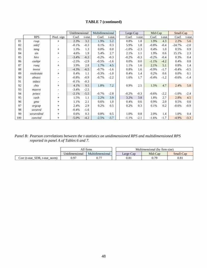
48

TABLE 7 (continued)

Panel B: Pearson correlations between the t-statistics on unidimensioned RPS and multidimensioned RPS

reported in panel A of Tables 6 and 7.

RPS Pred. sign Coef. t-stat. Coef. t-stat. Coef. t-stat. Coef. t-stat. Coef. t-stat.

81 rsup + 2.3% 3.2 1.9% 5.2 0.8% 1.8 1.9% 4.3 2.2% 5.6

82 stdcf - -0.1% -0.3 0.1% 0.3 5.9% 1.8 -0.8% -0.4 -24.7% -2.0

83 tang + 1.3% 1.3 0.0% 0.0 -1.0% -2.3 0.4% 1.0 0.5% 0.9

84 sin + 4.6% 1.9 5.4% 2.7 2.1% 1.1 1.9% 0.6 15.1% 2.3

85 hire - -3.4% -6.3 -0.2% -0.3 -0.2% -0.3 -0.2% -0.4 0.3% 0.4

86 cashpr - -2.5% -2.9 -0.5% -1.6 0.0% 0.0 -1.1% -4.2 0.4% 0.8

87 roaq + 3.9% 2.8 1.7% 4.5 1.1% 1.6 2.1% 5.1 0.8% 1.4

88 invest - -4.3% -6.5 -0.7% -1.6 0.8% 1.6 -0.9% -1.7 -0.4% -0.5

89 realestate + 0.4% 1.1 -0.3% -1.0 0.4% 1.4 0.2% 0.6 0.0% 0.1

90 absacc - -0.8% -0.9 -0.7% -2.2 1.6% 1.7 -0.4% -1.2 -0.6% -1.4

91 stdacc - -0.1% -0.3

92 chtx + 4.1% 9.5 1.8% 7.2 0.9% 2.5 1.5% 4.7 2.4% 5.8

93 maxret - -3.4% -2.5

94 pctacc - -2.1% -5.5 -0.7% -2.8 -0.2% -0.3 -0.6% -2.2 -1.0% -2.4

95 cash + 1.5% 1.1 2.2% 3.9 3.2% 3.8 1.8% 2.7 2.8% 4.5

96 gma + 1.1% 2.1 0.6% 1.0 0.4% 0.6 0.9% 2.0 0.5% 0.6

97 orgcap + 2.4% 2.9 0.2% 0.5 0.2% 0.3 0.1% 0.2 -0.6% -0.9

98 secured + -0.4% -1.6

99 securedind + 0.6% 0.3 0.8% 0.5 1.0% 0.8 2.0% 1.4 1.0% 0.4

100 convind + -5.0% -4.2 -2.5% -3.7 -1.1% -2.1 -1.6% -1.7 -4.9% -3.3

Unidimensional Multidimensional Large-Cap Mid-Cap Small-Cap

All firms Multimensional (by firm size)

Corr (t-stat_SDR, t-stat_norm) 0.97 0.77 0.81 0.79 0.81

Unidimensional Multidimensional Large-Cap Mid-Cap Small-Cap

49

TABLE 8

Comparison of multidimensioned results that use scaled decile ranked RPS with results where RPS

are winsorized and standardized to a mean of zero and standard deviation of 1. Coefficient estimates

in panel A are X100 and are annualized long/short hedge returns. Coefficient estimates in panel B

are X100 and then X12, making them the annualized returns to a one standard deviation increase in

the individual RPS. Absolute t-statistics 3.0 are color-highlighted by firm-size group.

Panel A: Scaled decile ranked RPS

Panel B: Normalized RPS

# RPS Pred. sign MALSRet t-stat. MALSRet t-stat. RPS t-stat. RPS t-stat. RPS t-stat.

1 sue + 20.3% 15.8 11.2% 14.2 sfe -10.1 retvol -10.5 sue 14.2

2 ear + 16.5% 16.6 9.3% 13.7 cash 5.0 sfe -9.7 ear 11.2

3 sfe + -8.1% -1.7 -14.5% -12.6 retvol -4.4 ear 9.1 turn 9.4

4 turn + 21.9% 9.1 23.4% 10.0 indmom 4.0 turn 7.8 mve -7.0

5 dolvol - 1.0% 1.5 -9.1% -9.3 ep 3.1 dolvol -6.9 rsup 6.5

6 rsup + 7.9% 3.8 6.7% 7.5 bm 3.0 roaq 6.5 dolvol -6.3

7 roaq + 13.2% 3.3 9.6% 7.1 rsup 6.0 sfe -6.2

8 retvol - -5.7% -1.0 -11.6% -6.6 sue 5.4 stdcf -6.2

9 indmom + 25.8% 7.3 7.2% 6.3 indmom 5.0 ep 5.7

10 aeavol + 8.0% 7.0 3.0% 5.7 cash 4.8 rd_mve 5.2

15 bm + 15.1% 4.5 8.2% 4.4 bm 3.0 bm 2.0 bm 2.0

52 mve - -6.5% -1.6 -9.0% -1.7 mve -1.7 mve -0.9 mve -7.0

70 mom12m + 9.8% 6.1 0.7% 0.7 mom12m -0.4 mom12m 0.4 mom12m 0.4

Mean adjusted R2 0.4% 6.0% 17.0%

10 largest multidimensional t-stats. 10 largest multidimensional t-stats.

9.0% 4.0%

Mean # obs. per regression 5,032 4,930 910 1,911 1,931

21

# abs{t-stat} 1.96 48 46 20 29 34

# abs{t-stat} 3.0 35 24 6 20

All firms Multimensional (by firm size)

Unidimensional Multidimensional Large-Cap Mid-Cap Small-Cap

Mean # obs. per regression

Mean adjusted R2

# RPS Pred. sign Coef. t-stat. Coef. t-stat. RPS t-stat. RPS t-stat. RPS t-stat.

1 ear + 6.2% 19.7 4.1% 16.1 sfe -6.5 ear 9.6 sue 14.1

2 sue + 6.6% 17.9 3.9% 14.6 indmom 4.9 retvol -7.8 ear 10.6

3 sfe + -1.6% -1.1 -3.3% -10.2 ep 4.5 sue 6.6 mve -9.7

4 indmom + 7.4% 7.3 2.3% 7.7 cash 3.8 indmom 6.4 aeavol 8.2

5 chtx + 4.1% 9.5 1.8% 7.2 retvol -3.6 sfe -6.3 ep 6.6

6 aeavol + 3.4% 9.7 1.6% 7.0 roaq 5.1 zerotrade -6.4

7 mve - -3.0% -2.2 -9.8% -5.8 chtx 4.7 indmom 6.0

8 ep + 0.7% 0.4 3.3% 5.4 ep 4.5 chtx 5.8

9 zerotrade + 1.0% 1.5 -2.8% -5.4 rsup 4.3 rsup 5.6

10 rsup + 2.3% 3.2 1.9% 5.2 chfeps 4.2 sfe -5.4

27 bm + 4.3% 4.9 1.6% 3.1 bm 2.4 bm 1.0 bm 0.5

7 mve - -3.0% -2.2 -9.8% -5.8 mve -1.8 mve -4.0 mve -9.7

39 mom12m + 2.6% 6.2 -0.9% -2.4 mom12m 0.5 mom12m -2.3 mom12m -1.4

53 roic + 1.2% 0.8 0.8% 1.4 roic 1.5 roic 0.5 roic 1.0

14 agr - -2.7% -6.4 -0.7% -2.5 agr -0.5 agr -1.8 agr -0.5

# abs{t-stat} 3.0 28 5 20 1934

All firms Multimensional (by firm size)

Mid-Cap Small-Cap

# abs{t-stat} 1.96 43 14 33 27

Unidimensional Multidimensional Large-Cap

51

10 largest multidimensional t-stats. 10 largest multidimensional t-stats.

4,930

7.0%

911

18.0%

5,032

0.3%

1,911

10.0%

1,931

5.0%

50

TABLE 9

The sets of RPS selected via panel LASSO regressions, using mean-adjusted monthly returns as

the dependent variable. Missing values are set equal to zero. RPS variables are ranked into

deciles (0-9) and divided by 9. Ranking is performed for sample used in regressions; i.e.

ranking for all firms and separately for large, mid-size, and small firms. Large-Cap are the

largest 1,000 companies by market cap; Mid-Cap are the next largest 2,000 companies; Small-

Cap are all remaining firms.

All firms Large-Cap Mid-Cap Small-Cap

1 sue ep ep mve

2 bm mom36m sue sue

3 mom36m mom1m chfeps bm

4 mom12m mom12m bm quick

5 sp sp mom6m saleinv

6 acc indmom sp turn

7 turn sfe acc indmom

8 nincr grltnoa turn dolvol

9 indmom roic indmom std_turn

10 dolvol agr sfe nanalyst

11 sfe chcsho grltnoa rd_mve

12 rd_mve chtx agr aeavol

13 aeavol maxret ear agr

14 agr cashpr chcsho

15 chcsho roaq ear

16 ear invest tang

17 roaq chtx stdacc

18 invest maxret maxret

19 maxret

51

TABLE 10

Tests of factor portfolio returns. Every month, for each of the 100 RPS listed in Table 1, firms

are ranked into deciles. Then, for each RPS decile and each month, an equally-weighted RPS

decile portfolio return is created using firms’ returns in the subsequent month, yielding a time

series of monthly portfolio returns for each of the 1,000 RPS decile combinations. For each

RPS decile, a time series regression of that RPS decile’s monthly portfolio returns on the factor

returns pertinent to one of four alternative factor models is then estimated: [1] the equally-

weighted market EW; [2] EW and the long/short hedge portfolio factor returns to market cap,

book-to-market and 12 month momentum; [3] EW and the factor returns to market cap, book-

to-market, profitability and asset growth; [4] the model that selects the five factor returns from

the set of 100 RPS-based factor returns with the highest time series adjusted R2. Then for each

RPS the mean absolute value of the regression intercepts and the mean adjusted R2 across the

10 deciles are calculated. Panel A reports descriptive statistics on these 100 mean absolute

intercepts and 100 adjusted R2 (one per RPS), while Panel B reports the frequency with which

the factors chosen by model [4] overlap with those of models [1] – [3].

Panel A: Performance of factor return models [1] – [4]

Panel B: Frequency with which factors chosen by model [4] overlap with those of models [1] – [3]

Statistic Min. Q1 Median Mean Q3 Max.

mean_absint 0.06% 0.18% 0.25% 0.27% 0.34% 0.51%

mean_adjR2 75.7% 90.1% 92.6% 91.7% 94.6% 98.8%

mean_absint 0.05% 0.11% 0.16% 0.19% 0.23% 0.91%

mean_adjR2 78.9% 93.9% 95.4% 94.5% 96.2% 98.8%

mean_absint 0.02% 0.11% 0.18% 0.20% 0.26% 0.81%

mean_adjR2 80.5% 94.9% 95.9% 95.2% 96.8% 98.9%

mean_absint 0.01% 0.08% 0.10% 0.12% 0.14% 0.45%

mean_adjR2 84.1% 96.7% 97.7% 97.0% 98.1% 99.7%

[4]

[2]

[3]

[1]

Factor Model

Equally-weighted market EW

EW and the long/short hedge

portfolio factor returns to firm size,

book-to-market and 12 month

momentum

EW and the factor returns to market

cap, book-to-market, profitability

and asset growth

The model that selects the five

factor returns from the set of 100

RPS-based factor returns with the

highest time series adjusted R2

Factor Model or Factor Return Frequency

Model [1] 51%

Model [2] 0%

Model [3] 0%

Firm size mve 17%

Book-to-market bm 4%

12-month momentum mom12m 2%

Profitability roic 5%

Asset growth agr 6%

52

FIGURE 1

Cumulative number of firm-specific return predictive signals (RPS) publicly reported in

Green, Hand and Zhang (2013) as having been discovered by accounting, finance and other

business academics, 1970-2010.

The number of RPS each year is the sum of the accounting-based, finance-based and other-based RPS reported in

Figure 1 of Green, Hand and Zhang (2013).

0

50

100

150

200

250

300

350

Cumulative # of ABTS vs. PBTS vs. OBTS, 1970 - 2010

Total RPS

53

FIGURE 2

Principal component factor analysis (PCA) of theset of 100 scaled decile ranked RPS, and of

the monthly RPS hedge returns. Only factors with an eigenvalue > 1.0 are shown. The x-axis is

the number of RPS factors and the y-axis is the variance explained by each factor

Panel A: Variance explained by PCA-derived factors in the set of 100 scaled decile ranked RPS

Panel B: Variance explained by PCA-derived factors of the monthly long/short biggest/smallest

decile RPS hedge returns

0.0

1.0

2.0

3.0

4.0

5.0

1 2 3 4 5 6 7 8 9 10 11 12 13 14 15 16 17 18 19 20 21 22 23 24 25 26 27 28 29

0

5

10

15

20

25

30

1 2 3 4 5 6 7 8 9 10 11 12 13 14

54

FIGURE 3

Out-of-sample hedge portfolio returns to alternative sets of RPS. Analysis is limited to large-

cap and mid-cap firms only; small-cap firms are excluded. Hedge portfolio returns are defined

as the sum of wt x rret each month, where wt = 2 x [pret]/[abs(pret]. pret is the predicted

mean-adjusted return based on estimating rolling 10-year regressions of mean-adjusted

returns on the relevant set of RPS, and then applying the estimated coefficients to the RPS in

place at the end of the 10-year window to estimate the next month’s predicted return. rret is

the realized return in the month immediately after the end of the 10-year estimation window.

Panel A: Statistics on monthly out-of-sample 2X-levered hedge portfolio returns, and their

associated annualized Sharpe ratios

Panel B: Ln(1+cumulative out-of-sample 2X gross levered hedge portfolio returns) for various sets

of multidimensioned RPS

Multidimensioned set of RPS t-stat. Min.10th

pctile

50th

pctileMean

90th

pctileMax.

Annualized

Sharpe

Carhart (1997): mve, bm, mom12m 4.8 -7.0% -2.3% 0.4% 0.8% 4.2% 9.0% 0.99

Fama & French (2013):

mve, bm, roic, agr, mom12m5.2 -9.2% -2.7% 0.7% 1.1% 4.9% 15.5% 1.08

ALL: All RPS (n = 91) 12.4 -11.8% 0.0% 2.1% 2.7% 6.3% 37.1% 2.58

Statistics on monthly out of sample hedge returns

55

FIGURE 4

Comparison of the out-of-sample hedge portfolio returns to the ALL RPS reported in Figure 4

with the distilled 10 RPS model. The RPS in the distilled 10 RPS model are: asset growth agr,

book-to-market bm, dollar trading volume dolvol, quarterly earnings announcement returns

ear, 12-month industry-adjusted returns indmom, 36 month momentum mom36m, quarterly

return on assets roaq, forecasted annual earnings sfe, unexpected quarterly earnings sue, and

share turnover turn. Exact RPS definitions are in Table 2. The RPS in the distilled model are

those that yield the largest adjusted R2 in a pooled time-series cross-sectional regression of 1-

month ahead mean-adjusted U.S. stock returns, Jan. 1980-Dec. 2012. Analysis is limited to

large-cap and mid-cap firms only. Hedge portfolio returns are constructed per Figure 3.

Panel A: Statistics on monthly out-of-sample 2X-levered hedge portfolio returns, and their

associated annualized Sharpe ratios

Panel B: Ln(1+cumulative out-of-sample 2X gross levered hedge portfolio returns) for various sets

of multidimensioned RPS

Multidimensioned set of RPS t-stat. Min.10th

pctile

50th

pctileMean

90th

pctileMax.

Annualized

Sharpe

ALL: All RPS (n = 91) 12.4 -11.8% 0.0% 2.1% 2.7% 6.3% 37.1% 2.58

TEN: Distilled 10 RPS model 14.1 -4.1% 0.2% 2.2% 2.5% 5.0% 32.0% 2.94

Statistics on monthly out of sample hedge returns