The Relative Profitability of Analysts’ Stock Recommendations: What Role Does Investor Sentiment Play?

Mark Bagnoli Purdue University

Michael Clement

University of Texas at Austin

Michael Crawley University of Texas at Austin

Susan Watts

Purdue University

October 26, 2009

Abstract: This study investigates whether analysts who respond to investor sentiment issue more or less profitable stock recommendations than their peers. We find that analysts, on average, issue more favorable stock recommendations when investor sentiment is more bullish. However, analysts whose stock recommendations are positively correlated with recent or future investor sentiment tend to issue less profitable recommendations than other analysts who follow the same firm and may focus solely on fundamentals such as earnings, cash flows, and discount rates. Our results suggest that some analysts recommend stocks based, in part, on signals that may affect price but that are not theoretically related to firms’ underlying intrinsic value. Thus, our results may help explain the findings of prior studies which document the failure of some analysts to fully incorporate their earnings forecasts into their stock recommendations.

We thank Larry Brown, Yonca Ertimur, Ross Jennings, Kevin Kobelsky, Bill Mayew, Philip Shane, Senyo Tse, Jenny Tucker, Richard Willis, Yong Yu, workshop participants at Baylor University and Purdue University, and conference participants at the 2009 American Accounting Association annual meeting for helpful comments.

1. Introduction

This study investigates whether analysts who respond to investor sentiment issue

more or less profitable stock recommendations than their peers. Baker and Wurgler

(2006) define investor sentiment as either a driver for the relative demand for speculative

investments or investors’ collective optimism or pessimism about stocks in general.

Although traditional valuation theory suggests that stock prices should be determined

solely by fundamentals (e.g. earnings, cash flows, and discount rates), recent empirical

research suggests that investor sentiment may also affect stock prices. For example,

Baker and Wurgler (2006, 2007) and Frazzini and Lamont (2008) find evidence that a

subset of stocks may be overpriced (underpriced) when investor sentiment is high (low).

If investor sentiment indeed leads asset prices, then analysts’ recognition and

treatment of sentiment may affect the relative profitability of their stock

recommendations. For example, an analyst may believe a particular stock is overvalued

based on her private estimate of the firm’s intrinsic value. However, the analyst may be

hesitant to issue a Sell recommendation if she believes that investor sentiment will

continue to exert upward pressure on asset prices in the near term. Moreover, the analyst

may actually issue a Buy recommendation if she believes that investors will become even

more bullish in the near future. If the analyst (1) correctly predicts a bullish (bearish)

shift in investor sentiment which ultimately increases (decreases) asset prices and (2)

issues a more favorable (unfavorable) recommendation in response, then the analyst’s

recommendation may be more profitable than the recommendations of her peers.

While responding to investor sentiment could lead to more profitable stock

recommendations, it could also lead to less profitable stock recommendations for several

1

reasons. First, forecasting investor sentiment is presumably costly (e.g. by requiring time

and resources that could be directed towards increasing forecast accuracy or serving

institutional clients). Thus, if sentiment’s impact on asset prices is not sufficiently large,

analysts may be wasting resources when considering investor sentiment. Second, even if

firm fundamentals remain constant and an analyst can perfectly predict future investor

sentiment, she must issue timely favorable (unfavorable) recommendations ahead of

bullish (bearish) periods of sentiment for her recommendations to be more profitable than

those of her peers. Thus, recommendation profitability may be reduced if analysts’

recommendation revisions are infrequent compared to shifts in investor sentiment, and

prior research suggests that the investment value of recommendations decreases after six

months (Womack 1996). Whether analysts are ultimately successful in increasing

recommendation profitability by incorporating investor sentiment is an empirical

question that we investigate in this study.1

Our research design classifies an individual analyst as responding to sentiment in

a given year if the recommendations she issues during the year are correlated with recent

or future sentiment after controlling for the analyst’s incentives and a proxy for the

analyst’s private estimate of the firm’s intrinsic value. In order to ascertain whether

analysts who respond to sentiment issue relatively more or less profitable stock

recommendations, we create a measure of relative recommendation profitability for each

analyst-firm-year. We determine relative recommendation profitability on a calendar

year basis by assigning an analyst “credit” based on her recommendation and the firm’s

return. For each day the analyst has a Buy (Strong Buy) recommendation outstanding,

1 We do not take a stand as to whether asset prices can deviate from fundamental value. Rather, we attempt to determine how analysts’ beliefs about investor sentiment are manifested within their recommendations and whether analysts who respond to sentiment issue more or less profitable recommendations.

2

the analyst receives daily credit equal to (double the) the stock’s daily return.

Conversely, for each day the analyst has a Sell (Strong Sell) recommendation

outstanding, the analyst’s daily credit is equal to (double) the negative of the stock’s daily

return. The analyst is awarded a daily risk free rate for days with an outstanding Hold

recommendation.2 We aggregate an analyst’s credit for a given firm-year and then

compare each analyst to other analysts who had a recommendation outstanding for the

same stock over the same calendar year.

Our measure of relative stock recommendation profitability is unique because it

controls for all firm and time effects by holding constant the environment facing all

analysts following a specific firm in a given year. Controlling for firm and time effects is

important for two reasons. First, prior research finds that the level and profitability of

analysts’ recommendations are correlated with firm characteristics. For example,

Jegadeesh et al. (2004) find that analysts make more favorable recommendations for

glamour stocks (i.e. stocks with positive momentum, high trading volume, and strong

sales growth), and such recommendations are less profitable. Second, Baker and Wurgler

(2007) find that investor sentiment affects some firms (e.g. young, small, and distressed

stocks) more than others. However, a firm’s characteristics in a given year are the same

for all analysts following the firm. Hence, the impact of the firm’s trading volume, sales

growth, size, age, etc. on the task of issuing profitable stock recommendations is constant

across analysts and controlled for through the use of relative performance evaluation.

Thus, all variation in our measure of relative recommendation profitability should be due

to analyst or recommendation characteristics rather than firm effects (e.g. whether a firm

2 Our performance measure is similar to the measure used by The Wall Street Journal when compiling the annual “Best on the Street” survey (The Wall Street Journal May 26, 2009). Our results are qualitatively similar when using alternative performance measures (see Section 5).

3

is a glamour or value stock) or time effects (e.g. whether the recommendation took place

during a bull or bear market or during a particular regulatory regime).

Next, we regress our measure of relative stock recommendation profitability on a

proxy for the analyst’s earnings forecasting ability, other analyst characteristics

previously shown to be associated with forecast accuracy and recommendation

profitability, a proxy for the boldness of the analyst’s recommendation (i.e. the degree to

which the analyst’s recommendation deviates from the consensus), and our measures for

whether the analyst’s recommendations are correlated with investor sentiment.

Our major findings are two-fold. First, we find that analysts, on average, issue

more favorable stock recommendations when investor sentiment is more bullish. This

finding suggests that some analysts’ recommendations are influenced by investor

sentiment and that at least a subset of analysts may view the task of issuing stock

recommendations as a Keynesian beauty contest (Keynes 1936).3 Said differently, some

analysts may recommend a stock based, in part, on how the analyst believes the market as

a whole will move in the future, as opposed to making a recommendation strictly based

on a comparison of the current market price to the analyst’s private estimate of the firm’s

intrinsic value.

Second, we find that analysts whose stock recommendations are positively

correlated with investor sentiment tend to issue relatively less profitable

recommendations than their peers covering the same firm in the same year. Additionally,

responding to investor sentiment appears to lower recommendation profitability when

3 Keynes described a beauty contest as a situation in which judges pick who they think other judges will pick rather than who they consider to be the most beautiful. Keynes originally applied this reasoning to stock prices (see also Allen et al. (2006) and Gao (2008) for formal models of this idea), but the concept also applies to the incorporation of investor sentiment into analyst recommendations.

4

stock recommendations are associated with past sentiment (i.e., analysts are “chasing”

sentiment) or future sentiment (i.e., analysts are predicting sentiment). Note, this finding

does not necessarily imply that analysts who respond to investor sentiment issue

unprofitable recommendations. In fact, recommendations issued by analysts who

respond to investor sentiment may be profitable on an absolute basis. Instead, our results

suggest that recommendations issued by analysts who respond to investor sentiment are

less profitable, on average, than recommendations issued by their peers (e.g., analysts

who may focus solely on fundamentals such as earnings, cash flows, and discount rates).

Our results also indicate that past relative recommendation profitability is a

significant driver of current relative recommendation profitability. This result suggests

that the ability to issue relatively profitable stock recommendations is at least partially

persistent, consistent with Mikhail et al. (2004) and Li (2005). Like Loh and Mian

(2006) and Ertimur et al. (2007), we also find that earnings forecasting ability and several

analyst characteristics associated with forecast accuracy contain explanatory power for

relative stock recommendation profitability.4 We extend the literature by showing that

bold recommendations, which may reflect a greater degree of analyst conviction, are

generally more profitable, and we also find that analyst teams tend to produce more

profitable recommendations than individual analysts.5

We believe our study makes several contributions to the literature. First, we find

that at least a subset of analysts issue more favorable stock recommendations when

4 For example, the forecasting literature predicts that earnings forecast accuracy increases with forecast frequency. Our results go further, however, and suggest relative recommendation profitability increases with forecast frequency even after considering the more accurate earnings forecast. 5 Interestingly, this benefit of teamwork contrasts with the result in Brown and Hugon (2008) that teams provide less accurate earnings estimates, and thus our results may provide a partial explanation for the existence of analyst teams.

5

investor sentiment is more bullish. Second, we show that the analysts who appear to

respond to investor sentiment tend to issue relatively less profitable stock

recommendations than their peers. Third, we introduce a new analyst-firm-year specific

measure of relative recommendation profitability that provides strong controls for both

firm and time effects and also allows us to directly assess each explanatory variable’s

relative contribution to relative recommendation profitability. Fourth, we demonstrate

that the boldness of the recommendation (i.e. the analyst’s conviction about the

recommendation) and whether the recommendation was issued by a team of analysts are

key contributors to relative recommendation profitability.

Our results should be of interest to researchers and a variety of capital market

participants. Given analysts’ role as information intermediaries, researchers seek to

understand the information and processes that analysts use when making stock

recommendations. Investors may also gain insights into how to use both analysts’

earnings forecasts and stock recommendations in concert with one another to maximize

the profitability of their investment strategies. Further, our results may help analysts

efficiently allocate their effort by helping analysts decide whether or not to devote costly

time and effort towards considering investor sentiment. Finally, brokerage firms could

find our methodology and results useful when hiring, training, evaluating, and

compensating analysts, particularly given recent regulatory developments which prevent

analyst compensation from being directly tied to investment banking revenues.

The remainder of the paper is structured as follows. Section 2 reviews the prior

literature, and Section 3 describes our model of the analyst’s stock recommendation task.

6

Section 4 outlines our research design. Section 5 describes the data and reports the

results, and Section 6 concludes.

2. Prior Research

Our study is related to two streams of literature. The first stream identifies

systematic differences in stock recommendation profitability across analysts and

investigates the determinants of these differences. The second stream investigates the

mapping of earnings forecasts into stock recommendations (i.e. how analysts utilize their

own earnings forecasts when making recommendations). We discuss each of the

literature streams and our contributions to the literature in more detail below.

Prior research documents that not only can investors profit from the

recommendations of analysts, but also that systematic differences in stock

recommendation profitability exist. For example, Barber et al. (2001) find that

purchasing (selling) stocks with the most (least) favorable recommendations yields

abnormal returns. Mikhail et al. (2004) and Li (2005) extend this finding by showing that

analysts whose recommendations earned the greatest abnormal returns in the past

continue to outperform in the future. Loh and Mian (2006) help explain differences in

recommendation profitability by showing that analysts who issue more accurate earnings

forecasts also issue more profitable stock recommendations.6 Ertimur et al. (2007) re-

examine this issue and find that, after controlling for expertise, more accurate analysts

make more profitable stock recommendations, but only for firms with value-relevant

earnings. Similarly, Mikhail et al. (2006) find that analysts who issue the most profitable

6 Hall and Tacon (2009) replicate this result but find that persistence in relative forecast accuracy is insufficient to allow investors to use historical forecast accuracy to identify those analysts whose current recommendations will be more profitable.

7

recommendations follow fewer industries, have better resources at their disposal, issue

their recommendations before their peers, and have a greater ability to predict which

firms will experience deterioration in their future performance.

A second related set of studies investigates the mapping of earnings forecasts into

stock recommendations. Bradshaw (2004) finds that analysts do not appear to generate

stock recommendations by using their own earnings forecasts as inputs into formal

present value models. Instead, he finds evidence that analysts rely on valuation heuristics

(e.g. using PEG ratios) to generate their recommendations. Ke and Yu (2009) assert that

if analysts seek to maximize the profitability of their stock recommendations, then this

inconsistency between analysts’ earnings forecasts and their stock recommendations may

represent a “transformational inefficiency”. The authors attempt to identify analyst

attributes related to the level of transformational inefficiency and suggest

transformational inefficiencies may result for several reasons. First, analysts may simply

be unable to efficiently transform their earnings forecasts into stock recommendations.

Second, analysts may manipulate recommendations to aid in the acquisition of private

information. Finally, analysts may be subconsciously affected by psychological biases.

Although frictions in the process of transforming earnings forecasts into stock

recommendations may exist, Groysberg et al. (2008a) show that the market for sell-side

financial analysts is liquid and characterized by high salaries and frequent performance

reviews. Hence, analysts who either are unable to transform their earnings forecasts into

stock recommendations or underperform their peers due to behavioral biases should be

eliminated from the market if a key criterion for success is the analyst’s recommendation

profitability. Consequently, we propose an alternative explanation for why

8

inconsistencies between analysts’ earnings forecasts and their stock recommendations

may arise. Given evidence that analysts are sensitive to investor sentiment when revising

their earnings forecasts (Clement et al. 2008) and the possibility that investor sentiment

affects asset prices, we postulate that analysts may be consciously attempting to

incorporate investor sentiment into their stock recommendations. In doing so, analysts’

stock recommendations may not be justified by their own earnings forecasts for the firm,

and analysts’ apparent transformational inefficiency may instead represent their attempt

to incorporate the impact of sentiment on asset prices into their recommendations.

We extend the literature by showing that some analysts appear to respond to

investor sentiment when issuing recommendations. However, recommendations issued

by those analysts tend to be relatively less profitable than recommendations issued by

other analysts who follow the firm. We also introduce a new analyst-firm-year specific

measure of relative recommendation profitability that controls for both firm and time

effects. Finally, we show that bold recommendations and recommendations issued by

teams of analysts are relatively more profitable. .

3. The Analyst’s Stock Recommendation Task

In this section we describe our model of the analyst’s stock recommendation task.

Although analysts’ objective functions are unobservable, prior research indicates analyst

reputation and compensation may be increasing in stock recommendation profitability.

For example, Emery and Li (2007) find that the probability of an analyst consistently

being classified as “Best on the Street” by The Wall Street Journal is increasing in stock

recommendation profitability. Additionally, while Groysberg et al. (2008b) find no

9

econometric relation between recommendation profitability and analyst compensation,

the authors provide anecdotal evidence that research directors at high-status investment

banks track and care about the stock recommendation profitability of their analysts.

We model an analyst focused on making the most profitable stock

recommendations possible as an agent who compares her expectation of the firm’s future

stock price with its current price.7 The analyst offers a Buy (Strong Buy)

recommendation when she expects the stock price increase to be large (very large), a Sell

(Strong Sell) recommendation when she expects the stock price decrease to be large (very

large) and a Hold recommendation otherwise. Differences in recommendations therefore

arise from differences in analysts’ expectations about future stock prices. We separate

the analyst’s expectation about the firm’s future stock price into two components: (1) the

analyst’s estimate of the firm’s intrinsic value and (2) the analyst’s expectation of all

other signals incremental to intrinsic value that may affect the firm’s stock price (at least

in the short run). Our analyses focus on investor sentiment as a signal that may affect a

firm’s stock price, but not its intrinsic value.

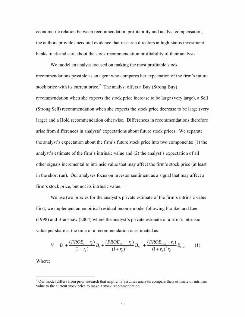
We use two proxies for the analyst’s private estimate of the firm’s intrinsic value.

First, we implement an empirical residual income model following Frankel and Lee

(1998) and Bradshaw (2004) where the analyst’s private estimate of a firm’s intrinsic

value per share at the time of a recommendation is estimated as:

222

121

)1()(

)1()(

)1()(

++

++

+−

++

−+

+−

+= tee

ett

e

ett

e

ett B

rrrFROE

Br

rFROEB

rrFROE

BV (1)

Where:

7 Our model differs from prior research that implicitly assumes analysts compare their estimate of intrinsic value to the current stock price to make a stock recommendation.

10

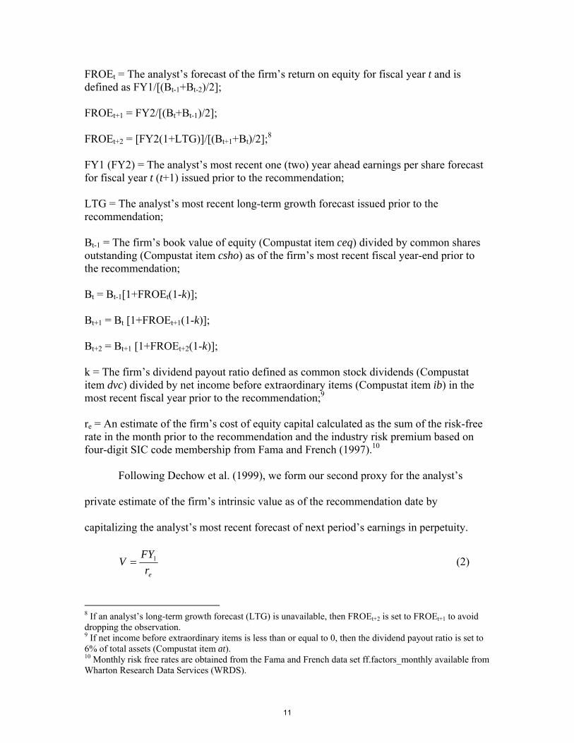
FROEt = The analyst’s forecast of the firm’s return on equity for fiscal year t and is defined as FY1/[(Bt-1+Bt-2)/2]; FROEt+1 = FY2/[(Bt+Bt-1)/2]; FROEt+2 = [FY2(1+LTG)]/[(Bt+1+Bt)/2];8 FY1 (FY2) = The analyst’s most recent one (two) year ahead earnings per share forecast for fiscal year t (t+1) issued prior to the recommendation; LTG = The analyst’s most recent long-term growth forecast issued prior to the recommendation; Bt-1 = The firm’s book value of equity (Compustat item ceq) divided by common shares outstanding (Compustat item csho) as of the firm’s most recent fiscal year-end prior to the recommendation; Bt = Bt-1[1+FROEt(1-k)]; Bt+1 = Bt [1+FROEt+1(1-k)]; Bt+2 = Bt+1 [1+FROEt+2(1-k)]; k = The firm’s dividend payout ratio defined as common stock dividends (Compustat item dvc) divided by net income before extraordinary items (Compustat item ib) in the most recent fiscal year prior to the recommendation;9 re = An estimate of the firm’s cost of equity capital calculated as the sum of the risk-free rate in the month prior to the recommendation and the industry risk premium based on four-digit SIC code membership from Fama and French (1997).10

Following Dechow et al. (1999), we form our second proxy for the analyst’s

private estimate of the firm’s intrinsic value as of the recommendation date by

capitalizing the analyst’s most recent forecast of next period’s earnings in perpetuity.

erFY

V 1= (2)

8 If an analyst’s long-term growth forecast (LTG) is unavailable, then FROEt+2 is set to FROEt+1 to avoid dropping the observation. 9 If net income before extraordinary items is less than or equal to 0, then the dividend payout ratio is set to 6% of total assets (Compustat item at). 10 Monthly risk free rates are obtained from the Fama and French data set ff.factors_monthly available from Wharton Research Data Services (WRDS).

11

The residual income method in Equation (1) has the theoretical advantage of

generating estimates that should equate to the firm’s true intrinsic value provided inputs

are accurate and the clean surplus relation is not violated. However, both assumptions

are somewhat problematic, and the residual income method imposes strict data

requirements that sharply reduce our sample size. The method in Equation (2) has the

advantage of maximizing our sample size, and both Dechow et al. (1999) and Liu et al.

(2002) find that capitalizations of analysts’ earnings forecasts better explain the cross-

section of observed prices than valuation estimates from more formal valuation models.

Next, we attempt to measure the analyst’s expectation of other signals that may

affect the firm’s stock price but not the firm’s intrinsic value. Specifically, we investigate

whether the analyst appears to respond to investor sentiment when making her stock

recommendations by estimating the following regression model:

Reci,j,t = α0 + α1LagReci,j,t + α2VPi,j,t + α3IBanki,t + α4TopTieri,t + α5MktSentt +

α6MktSentLagt + α7MktSentLeadt + νi,j,t (3)

Where:

Reci,j,t = Analyst i’s recommendation for firm j issued on day t. Recommendations from I/B/E/S are manipulated such that 5 = Strong Buy, 4 = Buy, 3 = Hold, 2 = Sell, and 1 = Strong Sell; LagReci,j,t = Analyst i’s previous recommendation for firm j;11 VPi,j,t = The proxy for analyst i’s private estimate of firm j’s intrinsic value as of the recommendation date scaled by firm j’s stock price at the end of the month prior to the recommendation; IBanki,t = One of two dummy variables that combine to measure the relative importance of investment banking business to analyst i’s broker as of the recommendation date. Our

11 We estimate Model (3) to investigate whether analyst recommendation levels are correlated with the level of investor sentiment. Although we include the lag of the analyst’s recommendation as an explanatory variable, we do not restrict the regression coefficient to equal 1. Thus, Model (3) remains a levels specification as opposed to a changes analysis.

12

measurement of the relative importance of investment banking to the broker is based on the rankings created by Carter and Manaster (1990) and modified by Loughran and Ritter (2004). The rankings range from 1 to 9 with higher values representing more prestigious underwriters with more dependence on investment banking revenues and a higher probability of conflicts of interest. IBank = 1 if the broker is ranked and the maximum ranking for the broker over the period 1993 to 2007 is greater than or equal to 1 and less than 9, and IBank = 0 otherwise; TopTieri,t = The second dummy variable that combines with IBank to measure the relative importance of investment banking business to analyst i’s broker. TopTier = 1 if the maximum ranking for the broker over the period 1993 to 2007 equals 9, and TopTier = 0 otherwise. Thus, TopTier brokers tend to be the largest and most prestigious underwriters with the greatest expected conflicts of interest; MktSentt = The monthly Baker and Wurgler (2006) investor sentiment index for the month of the recommendation; MktSentLagt = The average of the Baker and Wurgler (2006) investor sentiment index for the 3 months prior to the month of the recommendation; MktSentLeadt = The average of the Baker and Wurgler (2006) investor sentiment index for the 3 months subsequent to the month of the recommendation;12

We first estimate separate cross-sectional specifications of Model (3) where the

VP variable is constructed according to Equations (1) and (2). We expect α1, the

coefficient on LagRec, to be positive to the extent that analysts’ recommendations are

“sticky”. We also expect α2, the coefficient on VP, to be positive indicating that analysts’

recommendations are more bullish when their own private estimate of intrinsic firm value

is high relative to the firm’s current price. We make no predictions for IBank and

TopTier because Ertimur et al. (2007) show the effect of potential conflicts of interest on

recommendation levels depends on the regulatory regime in place at the time the

recommendation was made. Similarly, we make no predictions for the sentiment

variables because it is a priori unclear as to whether analysts’ recommendations are

12 Results for all empirical tests are quantitatively and qualitatively similar when using the average of the Baker and Wurgler (2006) investor sentiment index for the 6 months prior (subsequent) to the month of the recommendation to form the MktSentLag (MktSentLead) variables.

13

correlated with investor sentiment. A positive (negative) α6 coefficient in the cross-

section would indicate that analysts as a group issue more favorable (unfavorable)

recommendations when recent investor sentiment was more bullish. Similarly, a positive

(negative) α7 coefficient would suggest analysts as a group issue more favorable

(unfavorable) recommendations when future investor sentiment is more bullish.

We then re-estimate Model (3) for each analyst-year combination where the VP

variable is constructed using Equation (2) in order to prevent a loss of sample size and

statistical power. Estimating Model (3) for each analyst-year allows us to determine

whether an individual analyst appears to respond to investor sentiment when making

stock recommendations in a given year.13 We classify an analyst as responding to

investor sentiment by measuring whether or not her stock recommendations are

correlated with investor sentiment a given year. More specifically, we set a dummy

variable Correlate equal to 1 if either the α6 or α7 coefficients from Model (3) estimated

for a given analyst-year combination are significantly different from zero at the 5% level,

and Correlate is set to zero otherwise. We then match the analyst-year specific value for

the Correlate variable to each firm the analyst followed during the year. Lastly, we

determine whether characteristics previously shown to be associated with forecasting or

13 Model (3) implicitly treats investor sentiment as exogenous with respect to individual analysts. We maintain that endogeneity concerns are mitigated in our setting for several reasons. First, an analyst issuing recommendations for individual firms is a priori unlikely to influence investors’ collective optimism about the entire market, and the Baker and Wurgler (2006) investor sentiment index is constructed from market level proxies including the closed-end fund discount, New York Stock Exchange share turnover, the number and average returns on initial public offerings, and the dividend premium. Second, O’Brien and Tian (2008) fail to find evidence that analysts’ bullish recommendations on technology stocks contributed to the substantial price increases in the late 1990’s (a period of high sentiment as measured by Baker and Wurgler). Finally, if an analyst’s stock recommendations affect investor sentiment and investor sentiment influences prices, then one might expect the analyst’s recommendations to be more profitable than her peers. However, as we will later show, analysts who appear to respond to sentiment actually issue relatively less profitable stock recommendations.

14

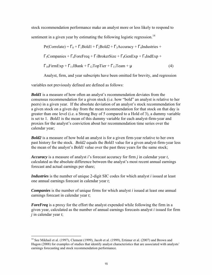
stock recommendation performance make an analyst more or less likely to respond to

sentiment in a given year by estimating the following logistic regression.14

Pr(Correlate) = Г0 + Г1Bold1 + Г2Bold2 + Г3Accuracy + Г4Industries +

Г5Companies + Г6ForeFreq + Г7BrokerSize + Г8GenExp + Г9IndExp +

Г10FirmExp + Г11IBank + Г12TopTier + Г13Team + μ (4)

Analyst, firm, and year subscripts have been omitted for brevity, and regression

variables not previously defined are defined as follows:

Bold1 is a measure of how often an analyst’s recommendation deviates from the consensus recommendation for a given stock (i.e. how “bold” an analyst is relative to her peers) in a given year. If the absolute deviation of an analyst’s stock recommendation for a given stock on a given day from the mean recommendation for that stock on that day is greater than one level (i.e. a Strong Buy of 5 compared to a Hold of 3), a dummy variable is set to 1. Bold1 is the mean of this dummy variable for each analyst-firm-year and proxies for the analyst’s conviction about her recommendation time series over the calendar year; Bold2 is a measure of how bold an analyst is for a given firm-year relative to her own past history for the stock. Bold2 equals the Bold1 value for a given analyst-firm-year less the mean of the analyst’s Bold1 value over the past three years for the same stock; Accuracy is a measure of analyst i’s forecast accuracy for firm j in calendar year t, calculated as the absolute difference between the analyst’s most recent annual earnings forecast and actual earnings per share; Industries is the number of unique 2-digit SIC codes for which analyst i issued at least one annual earnings forecast in calendar year t; Companies is the number of unique firms for which analyst i issued at least one annual earnings forecast in calendar year t; ForeFreq is a proxy for the effort the analyst expended while following the firm in a given year, calculated as the number of annual earnings forecasts analyst i issued for firm j in calendar year t;

14 See Mikhail et al. (1997), Clement (1999), Jacob et al. (1999), Ertimur et al. (2007) and Brown and Hugon (2008) for examples of studies that identify analyst characteristics that are associated with analysts’ earnings forecasting and stock recommendation performance.

15

BrokerSize is a measure of the size and resources available to the analyst’s broker, calculated as the number of analysts employed by analyst i’s broker who issue at least one annual earnings forecast during calendar year t; GenExp is a measure of the analyst’s general experience, calculated as the number of calendar years in which analyst i has issued at least one annual earnings forecast for any firm; IndExp is a measure of the analyst’s industry experience, calculated as the number of calendar years for which analyst i has issued at least one annual earnings forecast for any firm with the same 2-digit SIC code as firm j; FirmExp is a measure of the analyst’s firm-specific experience, calculated as the number of calendar years for which analyst i has issued at least one annual earnings forecast for firm j; Team is a dummy variable set to 1 if the recommendation is made by a team of analysts as opposed to an individual analyst, and Team = 0 otherwise. Teams of analysts were identified manually based on the analyst name field from I/B/E/S. Teams may include industry groups (e.g. Airlines), country groups (e.g. Norway), or other groups (e.g. Smith, Jones, and Walker);

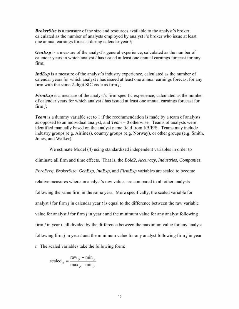
We estimate Model (4) using standardized independent variables in order to

eliminate all firm and time effects. That is, the Bold2, Accuracy, Industries, Companies,

ForeFreq, BrokerSize, GenExp, IndExp, and FirmExp variables are scaled to become

relative measures where an analyst’s raw values are compared to all other analysts

following the same firm in the same year. More specifically, the scaled variable for

analyst i for firm j in calendar year t is equal to the difference between the raw variable

value for analyst i for firm j in year t and the minimum value for any analyst following

firm j in year t, all divided by the difference between the maximum value for any analyst

following firm j in year t and the minimum value for any analyst following firm j in year

t. The scaled variables take the following form:

jtjt

jtijtijt minmax

minrawscaled

−

−=

16

Thus, scaled variables are restricted to the interval [0,1] with greater scaled values

indicating higher relative values (e.g. a scaled GenExp value of 1 means the analyst was

the most experienced analyst following firm j in year t). All remaining variables remain

unscaled because they are either dummy variables (IBank, TopTier, and Team) or are

already restricted to the interval [0,1] (Bold1).

4. The Determinants of Stock Recommendation Profitability

Now we turn to the task of identifying the determinants of relative stock

recommendation profitability. In order to identify the determinants of relative stock

recommendation profitability and to determine whether analysts who respond to investor

sentiment issue more or less profitable stock recommendations than their peers, we

estimate the following regression model:

Money = β0 + β1LagMoney + β2Bold1 + β3Bold2 + β4MktSentLag1 +

β5MktSentLag2 + β6MktSentLead1 + β7MktSentLead2 + β8Accuracy +

β9Industries + β10Companies + β11ForeFreq + β12BrokerSize + β13GenExp

+ β14IndExp + β15FirmExp + β16IBank + β17TopTier + β18Team + ε (5)

Analyst, firm, and year subscripts have been omitted for brevity, and regression

variables not previously defined are defined as follows:

Money is our measure of the relative profitability of analyst i’s stock recommendation for firm j in calendar year t which is calculated as follows. Each day for a given stock for which an analyst has a stock recommendation outstanding, the analyst is awarded a daily “credit” based on her outstanding recommendation and the stock’s daily return. If the analyst has a Buy (Sell) recommendation outstanding, the analyst receives credit equal to the stock’s return (the negative of the stock’s return) for that day. If the analyst has a Strong Buy (Strong Sell) recommendation outstanding, the analyst receives credit equal to double the stock’s return (double the negative of the stock’s return) for that day. In other words, a Buy (Sell) recommendation for a given stock on a given day yields credit to the analyst as if the analyst was long (short) one share of the firm’s stock. Similarly, a

17

Strong Buy (Strong Sell) generates credit for the analyst as if the analyst was long (short) two shares of the firm’s stock. If the analyst had a Hold recommendation outstanding, the analyst’s daily credit is set to an amount that would equate to a constant annual risk free rate of 3%. Each of analyst i’s daily credits for firm j are arithmetically summed for calendar year t to form an analyst-firm-year observation for the Money variable; LagMoney is the relative profitability of the analyst’s stock recommendation for the same firm from the prior calendar year (i.e. the relative profitability of analyst i’s stock recommendation for firm j over calendar year t-1); MktSentLag1 is the first of four dummy variables that measure whether an individual analyst’s recommendations were correlated with investor sentiment in a given year. MktSentLag1 = 1 if the α6 coefficient from regression Model (3) is positive and significant at the 5% level for a given analyst-year combination, and MktSentLag1 = 0 otherwise. In other words, a value of 1 for MktSentLag1 indicates analyst i issued more favorable recommendations in year t when recent investor sentiment was more bullish (i.e. the analyst was “chasing” investor sentiment for that year); MktSentLag2 is a dummy variable set to 1 if the α6 coefficient from regression Model (3) is negative and significant at the 5% level for a given analyst-year combination, and MktSentLag2 = 0 otherwise. A value of 1 for MktSentLag2 indicates analyst i issued less favorable recommendations in year t when recent investor sentiment was more bullish (i.e. the analyst was a contrarian with respect to past investor sentiment); MktSentLead1 is a dummy variable set to 1 if the α7 coefficient from regression Model (3) is positive and significant at the 5% level for a given analyst-year combination, and MktSentLead1 = 0 otherwise. A value of 1 for MktSentLead1 indicates analyst i issued more favorable recommendations in year t when future investor sentiment was more bullish, which may be consistent with the analyst predicting future investor sentiment and incorporating future sentiment into her recommendations; MktSentLead2 is a dummy variable set to 1 if the α7 coefficient from regression Model (3) is negative and significant at the 5% level for a given analyst-year combination, and MktSentLead2 = 0 otherwise. A value of 1 for MktSentLead2 indicates analyst i issued less favorable recommendations in year t when future investor sentiment was more bullish;

We estimate Model (5) using standardized dependent and independent variables

in order to eliminate firm and time effects and to discern the relative contribution of each

variable to the relative profitability of stock recommendations. Because (1) we expect

earnings forecasts to be inputs to recommendations; (2) some of the independent

variables in Model (5) have been previously shown to be associated with forecast

18

accuracy; and (3) forecast accuracy has previously been shown to be positively associated

with stock recommendation profitability, we predict that the coefficients will have the

same signs that they would have in explaining forecast accuracy. For example, we expect

positive coefficients for Accuracy (β8), ForeFreq (β11), BrokerSize (β12), GenExp (β13),

IndExp (β14), and FirmExp (β15), and negative coefficients for Industries (β9) and

Companies (β10) based on Clement (1999) and Jacob et al. (1999).

We also predict a positive coefficient for LagMoney (β1) based on Mikhail et al.

(2004) and Li (2005) who document persistence in recommendation profitability.

Clement and Tse (2005) find bold earnings forecast revisions (revisions that move away

from the consensus forecast) to be more accurate than herding forecast revisions

(revisions that move toward the consensus forecast), and thus we anticipate positive

coefficients for Bold1 (β2) and Bold2 (β3) if an analogous relation holds for

recommendations. Ertimur et al. (2007) find that non-conflicted analysts better translate

accurate earnings forecasts into profitable recommendations, and thus we expect negative

coefficients for IBank (β16) and TopTier (β17). We make no prediction for the sign of the

Team (β18) coefficient on because Brown and Hugon (2008) find that teams are less

accurate at forecasting earnings but issue forecasts earlier, and it is unclear how a team’s

tradeoff between timeliness and accuracy of earnings forecasts translates into

recommendation profitability. However, because earnings forecasts made by teams differ

from those made by individual analysts, we expect their recommendation profitability to

differ as well.

We also make no directional predictions for the sign of the coefficients on the

variables measuring the correlation between analysts’ recommendations and investor

19

sentiment. If investor sentiment affects asset prices, then we might expect the

recommendations of analysts who accurately predict future investor sentiment to be more

profitable. However, analyst effort expended analyzing investor sentiment could reduce

recommendation profitability to the extent that considering sentiment is costly (e.g. by

requiring time and resources that could be directed towards increasing forecast accuracy

or serving institutional clients) or if recommendation changes are not made in a timely

fashion to anticipate shifts in investor sentiment. Similarly, we might expect analysts

who are reacting to (or “chasing”) prior investor sentiment rather than predicting future

sentiment to suffer from a transformational inefficiency as suggested by Ke and Yu

(2009), leading such analysts to issue less profitable recommendations.

There are three important points to note about Model (5). First, our measure of

stock recommendation profitability, Money, is a relative performance measure. That is,

we compare the profitability of the analyst’s stock recommendation to the profitability of

other analysts who had an outstanding recommendation for the same stock during the

same period. This feature of the research design has the benefit of controlling for all

common firm and time effects that would affect the difficulty in making profitable stock

recommendations, such as firm size, analyst following and market-wide shocks. Second,

our measure of relative recommendation profitability is analyst-firm-year specific (as

opposed to being only analyst specific) which may allow investors to better maximize

their portfolio returns by identifying the best analysts for specific stocks. For example, in

contrast to previous studies, our methodology allows identification of an analyst who

may consistently make profitable stock recommendations for one firm or industry while

also consistently making poor recommendations for other firms or industries. Third,

20

because we use standardized dependent and independent variables we can comment on

each variable’s relative contribution to relative stock recommendation profitability.

In summary, we believe our research design allows us to answer several questions

that are important to researchers and practitioners. First, the results can help researchers

better understand how analysts transform their earnings forecasts into stock

recommendations. Second, our results could be useful to investors who must decide how

to use analysts’ earnings forecasts and stock recommendations in concert with one

another to make investment decisions. Third, the results should help identify whether

analyst team affiliation and the analyst’s degree of conviction contribute to relative

recommendation profitability. Finally, and perhaps most importantly, the study should

shed light on whether analysts’ who appear to respond to investor sentiment issue more

or less profitable stock recommendations than their peers.

5. Data and Empirical Results

All data used in this study are publicly available. Stock recommendation and

earnings forecast data are obtained from I/B/E/S.15 All price and return data are from The

Center for Research in Security Prices (CRSP) database, and necessary data for the

residual income model are from Compustat. Monthly investor sentiment data are

available on Professor Jeffrey Wurgler’s website at http://pages.stern.nyu.edu/~jwurgler.

Reputation rankings for brokerage houses as created by Carter and Manaster (1990),

modified by Loughran and Ritter (2004), and used by Ertimur et al. (2007) are available

on Professor Jay Ritter’s website at http://bear.cba.ufl.edu/ritter/ipodata.htm.

15 We use the corrected version of the I/B/E/S recommendation file (see Ljungqvist et al. 2009).

21

Our sample begins with all stock recommendations on the I/B/E/S detail file

beginning in 1994, the first full year of I/B/E/S recommendation coverage. To be

included in the sample, we require that an analyst have a recommendation outstanding for

the firm for all trading days within a calendar year, be associated with a brokerage house,

and have issued an annual earnings forecast for the same firm within the same calendar

year. Our methodology evaluates analysts’ recommendation profitability relative to all

other analysts following the same firm in the same year, and we therefore exclude

instances where there is only one analyst following a firm and where there is no between-

analyst variation in any of the primary regression variables for a given firm-year. Our

sample period ends in 2005, the last year in which Baker and Wurgler (2006) monthly

sentiment data are publicly available. Requiring all regression variables for Model (5)

described in the previous section to be non-missing results in a final sample of 107,826

analyst-firm-year observations from 1995 to 2005.

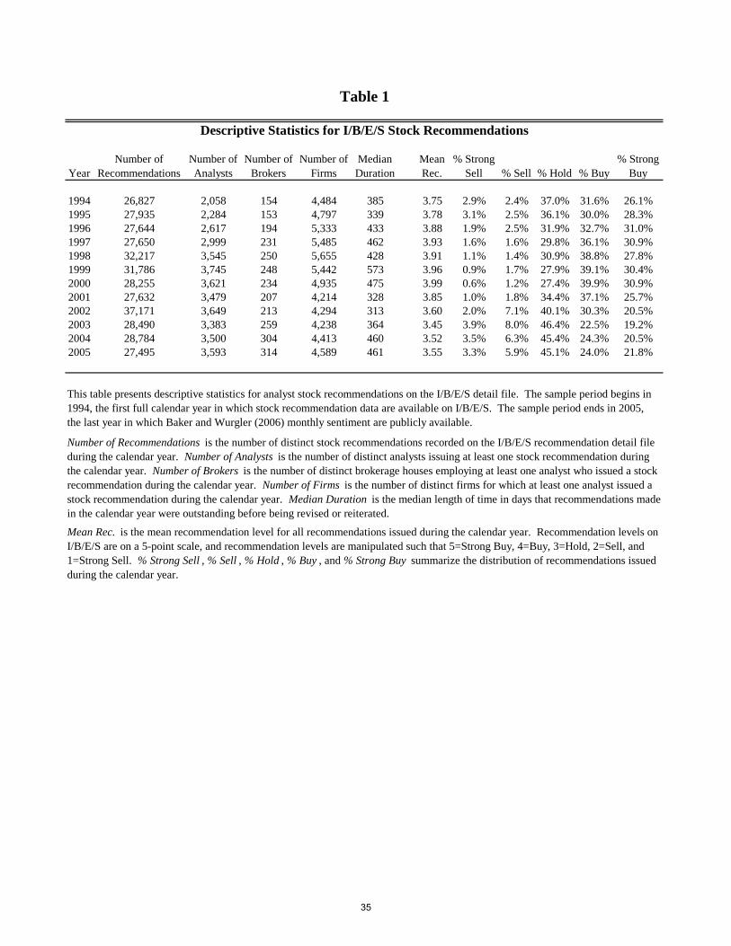
Table 1 provides descriptive statistics for I/B/E/S stock recommendations over

time. There is a general upward trend in the number of recommendations, analysts, and

brokers from 1994 to 2005. In contrast, there has been a reduction in the mean

recommendation level and a change in the distribution of recommendations over the same

period. The percentage of all recommendations issued as a Buy steadily climbs from

31.6% in 1994 to 39.9% in 2000 before declining to 24% in 2005. Similarly, the

percentage of recommendations issued as a Strong Buy reaches a high of 30.9% in 2000

before declining to 21.8% in 2005. The bearish shift in the distribution of

recommendations may have been precipitated by the Global Research Settlement reached

on April 23, 2003 which required brokerages to publish the distribution of their

22

recommendations. After the enforcement action, the percentage of recommendations

issued as a Hold consistently exceeds 45%, and over 54% are issued as a Hold, Sell, or

Strong Sell. Finally, the median recommendation duration exhibits no clear pattern over

the sample period. However, the median recommendation duration ranges from 313 days

to 573 days suggesting recommendation revisions are relatively infrequent events,

particularly compared to the frequency of analysts’ earnings forecast revisions.16

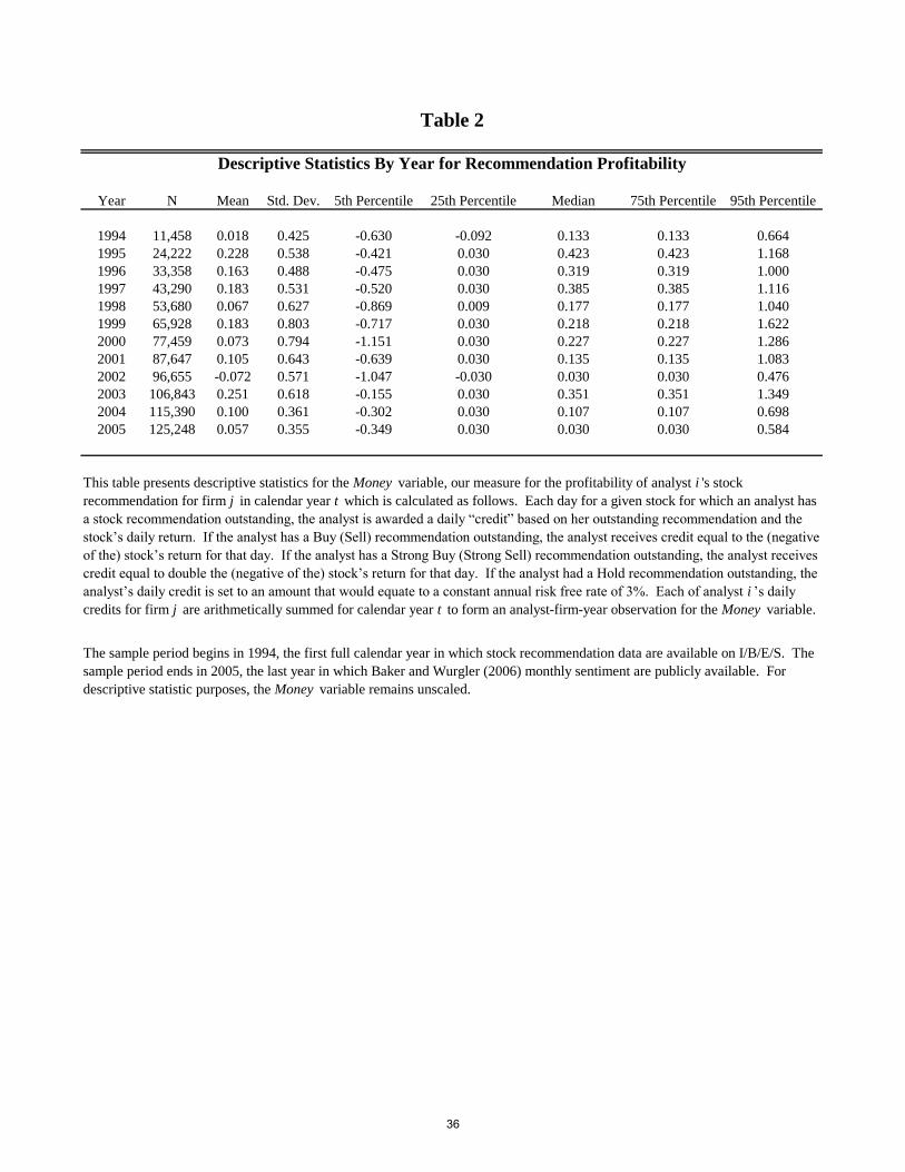
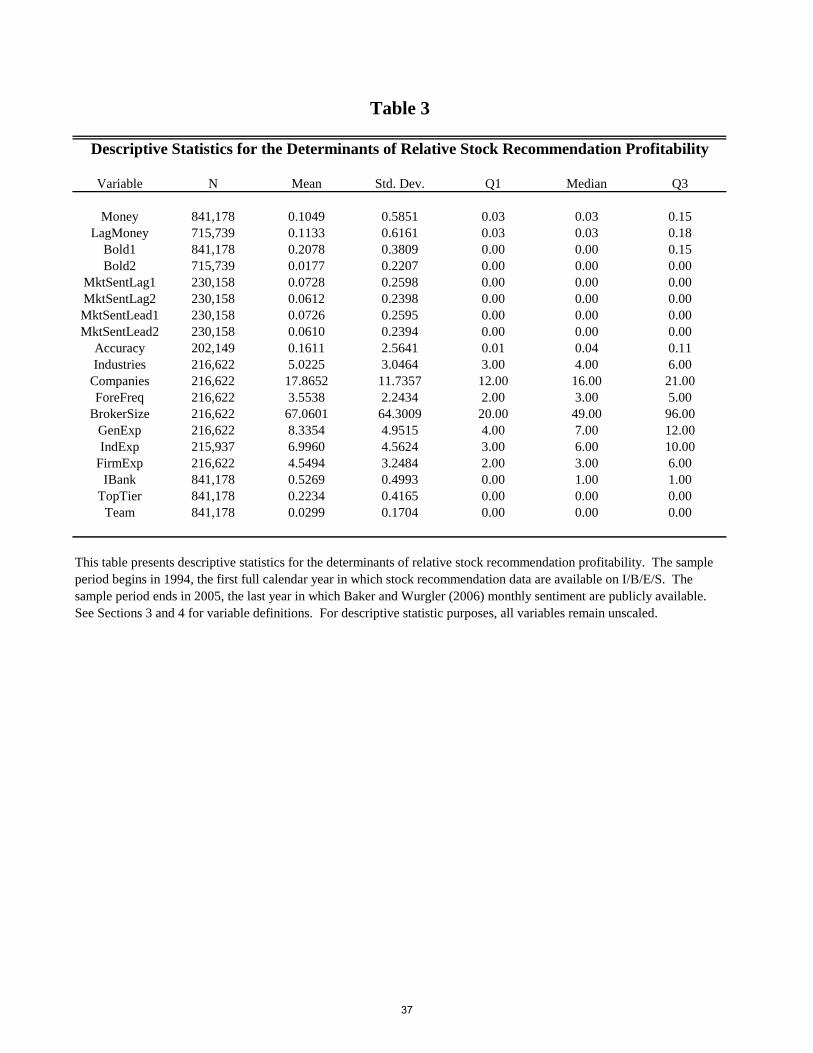
Tables 2 and 3 present descriptive statistics for the unscaled regression variables.

Table 2 shows the Money variable varies between -0.072 and 0.251 across years

suggesting there is significant variation in recommendation profitability for our model to

explain. In addition, the large 75th an 90th percentile values for Money suggest that any

methodology allowing investors to better ex-ante identify the analysts most likely to issue

the most profitable stock recommendations may allow investors to improve upon the

returns identified in previous studies. Notably, the mean for the Money variable

presented in Table 3 would loosely approximate a portfolio return of 10.5% if an investor

followed the recommendations of the mean analyst over the sample period. However,

values for our Money variable will not exactly equate to an investment return because our

methodology implies daily portfolio rebalancing and ignores transactions costs.

For the explanatory variables from the earnings forecasting literature, the means

presented in Table 3 are consistent with prior studies. For example, the average analyst

has approximately 8 years of general experience, follows nearly 18 companies across 5

industries, and issues almost 4 annual earnings forecasts per firm each year.

Additionally, approximately 52.7% (22.3%) of the observations consist of

16 As described above, we exclude observations where the analyst did not issue an annual earnings forecast for the firm in a year. We also include a variable which proxies for the level of effort the analyst expended while following the firm in the year to further minimize the impact of any stale recommendations.

23

recommendations made by analysts at brokers classified as an IBank (TopTier), and

analyst teams constitute around 3% of all observations in our sample. Further, 20.8% of

the recommendations are bold relative to the consensus, and 1.8% are bold relative to the

analyst’s prior recommendations. Perhaps most notably, 26.8% of observations contain

recommendations that appear to be correlated with investor sentiment.

Table 4 presents the cross-sectional regression results from Model (3) which

examines whether analysts’ stock recommendations as a whole are correlated with

investor sentiment. Panel A reports results where the proxy for the analyst's private

estimate of the firm's intrinsic value is calculated using the residual income model

described by Equation (1). Panel B reports results where the proxy for the analyst's

private estimate of the firm's intrinsic value is calculated by capitalizing the analyst's 1-

year ahead earnings forecast in perpetuity as described by Equation (2). Results are

consistent, both statistically and economically, across both specifications, and we discuss

the Panel A results.

As expected, the coefficient on LagRec is positive and significant indicating

analysts’ recommendations are “sticky”, and the positive and significant coefficient on

the VP variable of 0.141 indicates analysts’ recommendations are more bullish when the

analyst perceives the firm’s intrinsic value to be high relative to the current price. Thus,

the analyst’s current recommendation is influenced by her views about the firm and her

perception of the firm’s current intrinsic value. Somewhat surprisingly, the coefficient on

TopTier of -0.076 is significantly negative indicating analysts’ actually issue more

bearish recommendations when ex-ante expected conflicts of interest are greater.

However, untabulated results show the coefficient on the TopTier variable is only

24

negative and significant after the Global Research Settlement suggesting the enforcement

action may have reduced the effect of analysts’ conflicts of interest or increased the

perceived cost of appearing to issue overly optimistic recommendations.

Turning to the relation between investor sentiment and analysts’ stock

recommendations, the significant coefficient on the MktSentLag variable of 0.067

indicates analysts, on average, tend to issue more favorable recommendations when

investor sentiment over the prior 3 months has been more bullish. Similarly, the

significant coefficient on MktSentLead of 0.122 indicates analysts tend to issue more

favorable recommendations when future investor sentiment is more bullish. The positive

coefficient on MktSentLead suggests that at least a subset of analysts may be able to

predict future investor sentiment, and such behavior may partially explain why analysts

appear to fail to fully convert their earnings forecasts into stock recommendations.

While the results in Table 4 suggest analysts as a whole tend to both “chase” and

predict investor sentiment, it is also important to identify the characteristics that make an

individual analyst more or less likely to respond to sentiment in a given year. Table 5

presents the results of our logistic regression designed to determine which analyst

characteristics are associated with an individual’s propensity to attend to sentiment. In

order to interpret the impact of a one unit change in an independent variable on the

probability that the analyst's stock recommendations are correlated with investor

sentiment in a year, we focus on the marginal effects. Because marginal effects are

nonlinear functions of the parameter estimates and the levels of the independent

variables, we compute the marginal effect of each variable at each observation and report

the average across observations.

25

The results in Table 5 suggest that the most statistically and economically

significant variable in influencing whether an analyst’s recommendations are correlated

with investor sentiment in a given year is the number of companies followed. The

marginal effect associated with the Companies variable of 0.08 indicates that amongst

analysts following the same firm in the same year, the analyst following the most

companies is approximately 8% more likely to respond to investor sentiment compared to

the analyst who follows the least number of companies. Similarly, the probability that an

analyst’s stock recommendations are correlated with investor sentiment is increasing in

both the number of industries followed and the number of earnings forecasts issued.

Collectively, these results suggest that analysts who follow more firms and cover a wider

variety of industries may be more likely to incorporate signals that might affect price but

that are not theoretically related to intrinsic value when developing their

recommendations. Moreover, analyst teams and analysts facing potential conflicts of

interest are more likely to respond to sentiment while analysts with more firm-specific

experience are less likely to respond to sentiment.

Finally, Table 6 identifies the determinants of relative stock recommendation

profitability. Because we use standardized variables, the magnitude of the regression

coefficients allows us to determine the relative contributions of each variable to relative

recommendation profitability. Our results show that the variable with the largest impact

on relative recommendation profitability is past relative recommendation profitability

(LagMoney) with a coefficient of 0.089. Consistent with Mikhail et al. (2004) and Li

(2005), this result suggests that the ability to issue profitable stock recommendations is

somewhat persistent. We extend the literature by showing that the analyst’s level of

26

conviction about her recommendation is a key determinant of recommendation

profitability. Interestingly, the coefficient on Bold1 (0.063) is positive while the

coefficient on Bold2 (-0.015) is negative. This suggests that recommendations deviating

from the consensus tend to be relatively more profitable, but that recommendations which

are bolder than the analyst’s own prior recommendations are relatively less profitable.

The next most important variable is team designation (Team) indicating whether

the recommendation was issued by a team as opposed to by an individual analyst. The

positive and significant coefficient on Teams (0.021) suggests teams of analysts issue

more profitable stock recommendations and provides an interesting contrast to the

finding in Brown and Hugon (2008) that teams’ forecasting performance is worse. This

differential impact of being part of a team on forecasting accuracy and recommendation

profitability signifies that accurately forecasting earnings and issuing profitable stock

recommendations may require two separate but related skill sets and teams appear to

have an advantage in stock picking.

Collectively, the variables measuring the correlation between an analyst’s

recommendations and investor sentiment contain the next most explanatory power for

relative stock recommendation profitability. The significantly negative coefficient on

MktSentLag1 (-0.010) suggests that analysts whose recommendations are positively

correlated with recent investor sentiment tend to issue relatively less profitable

recommendations. This result is consistent with Baker and Wurgler (2006) and Frazzini

and Lamont (2008) who find that stocks tend to underperform after periods of bullish

sentiment. Further, this analyst behavior of chasing investor sentiment may also represent

a transformational inefficiency as outlined by Ke and Yu (2009). Similarly, the

27

significantly negative coefficient on MktSentLead1 (-0.011) suggests that analysts whose

recommendations are positively correlated with future investor sentiment tend to issue

relatively less profitable recommendations. This result is consistent with both

considering sentiment being costly and with analysts’ recommendation revisions not

being timely compared to shifts in investor sentiment. Taken together, these results

suggest that the average analyst is unable to efficiently predict and incorporate investor

sentiment into their stock recommendations.

Consistent with our predictions, earnings forecasting ability (Accuracy), earnings

forecast frequency (ForeFreq), and industry experience (IndExp) are all positively related

to relative recommendation profitability. However, in contrast to our prediction, the

employer size variable (BrokerSize) is negatively associated with relative

recommendation profitability. This result is surprising because employer size is

positively associated with forecast accuracy. Future research may provide a more

rigorous investigation into this interesting contrast, but one possible explanation is that

analysts who are employed at big brokers may have access to managers’ private

information that helps them forecast earnings but not stock prices.

The last set of statistically significant variables captures potential conflicts of

interest facing the analyst. The positive coefficient on IBank of 0.005 indicates that

analysts working for brokers with investment banking operations tend to issue more

profitable stock recommendations. However, consistent with Ertimur et al. (2007), we

find that analysts working for the most prestigious TopTier underwriters issue less

profitable stock recommendations on average.

28

We perform two sensitivity checks related to our measure of relative stock

recommendation profitability (results untabulated). First, we adjust the construction of

the Money variable such that an analyst with an outstanding Strong Buy recommendation

receives daily credit equal to double the stock’s daily return less a daily risk free rate.

This adjustment supposes that a hypothetical investor purchases twice as many shares in

response to a Strong Buy recommendation as compared to a Buy recommendation and

that those extra shares are financed by shorting the risk-free asset. Hence, the

recommendation profitability for an analyst with an outstanding Strong Buy

recommendation is based on the same endowment as the recommendation profitability

for an analyst with an outstanding Buy recommendation for the same stock. All results

remain quantitatively and qualitatively unchanged. Second, although Fama (1998) argues

for the use of arithmetic return measures in order to avoid potential extreme skewness

associated with compounded monthly returns, we also construct the Money variable by

geometrically aggregating an analyst’s credits for a given firm-year. Analysts whose

stock recommendations are positively correlated with recent or future investor sentiment

continue to appear to issue relatively less profitable recommendations.

6. Conclusion

This study investigates whether analysts whose stock recommendations are

correlated with recent or future investor sentiment issue more or less profitable

recommendations than their peers. We find that analysts, on average, issue more

favorable stock recommendations when recent and future investor sentiment is more

bullish. Hence, some analysts appear to recommend stocks based, in part, on signals that

29

may affect price but that are not theoretically related to firms’ underlying intrinsic value

as opposed to making a recommendation strictly based on a comparison of the current

market price to the analyst’s private estimate of the firm’s intrinsic value.

Our research design utilizes an analyst-firm-year specific measure of relative

stock recommendation profitability that provides strong controls for firm and time effects

and allows us to assess each analyst and recommendation characteristic’s relative

contribution to relative recommendation profitability. Consistent with prior research, we

show that earnings forecasting ability and several analyst characteristics associated with

forecast accuracy also have explanatory power for relative stock recommendation

profitability. We extend the literature by demonstrating that the analyst’s level of

conviction about her recommendation and whether the analyst is a member of a team are

also key determinants of relative recommendation profitability.

Finally, and perhaps most interestingly, we find that analysts whose stock

recommendations are positively correlated with recent or future investor sentiment tend

to issue relatively less profitable recommendations. Additionally, responding to investor

sentiment appears to lower relative recommendation profitability whether the analyst

seems to be chasing past sentiment or predicting future sentiment. However, our results

do not necessarily imply that analysts who respond to investor sentiment issue

unprofitable stock recommendations. In fact, recommendations issued by analysts who

respond to investor sentiment may be profitable on an absolute basis. Our results merely

suggest that recommendations issued by analysts who respond to investor sentiment are

less profitable, on average, than recommendations issued by their peers (e.g. analysts who

may focus solely on fundamentals such as earnings, cash flows, and discount rates).

30

Our results should be of interest to researchers and a variety of capital market

participants. Given analysts’ role as information intermediaries, researchers seek to

understand the information and processes that analysts use when making stock

recommendations. Investors may also gain insights into how to use both analysts’

earnings forecasts and stock recommendations in concert with one another to maximize

the profitability of their investment strategies. Further, our results may help analysts

efficiently allocate their effort by helping analysts decide whether or not to devote costly

time and effort towards considering investor sentiment. Finally, brokerage firms could

find our methodology and results useful when hiring, training, evaluating, and

compensating analysts, particularly given recent regulatory developments which prevent

analyst compensation from being directly tied to investment banking revenues.

31

References

Allen, F., S. Morris, and H.S. Shin. 2006. Beauty Contests and Iterated Expectations in Asset Markets. Review of Financial Studies 19: 719-752.

Baker, M., and J. Wurgler. 2006. Investor Sentiment and the Cross-Section of Stock Returns. Journal of Finance 61: 1645-1680.

Baker, M., and J. Wurgler. 2007. Investor Sentiment in the Stock Market. Journal of Economic Perspectives 21: 129-151.

Barber, B., B. Lehavy, M. McNichols, and B. Trueman. 2001. Can Investors Profit from the Prophets? Security Analyst Recommendations and Stock Returns. Journal of Finance 56: 531-563.

Bradshaw, M.T. 2004. How Do Analysts Use Their Earnings Forecasts in Generating Stock Recommendations? The Accounting Review 79: 25-50.

Brown, L., and A. Hugon. 2008. Team Earnings Forecasting. Review of Accounting Studies (forthcoming).

Carter, R., and S. Manaster. 1990. Initial Public Offerings and Underwriter Reputation. Journal of Finance 45: 1045-1067.

Clement, M. 1999. Analyst Forecast Accuracy: Do Ability, Resources, and Portfolio Complexity Matter? Journal of Accounting and Economics 27: 285-303.

Clement, M., J. Hales, and Y. Xue. 2008. Understanding Analysts’ Use and Under-use of Stock Returns and Other Analysts’ Forecasts when Forecasting Earnings. Working paper, University of Texas at Austin.

Clement, M., and S. Tse. 2005. Financial Analyst Characteristics and Herding Behavior in Forecasting. Journal of Finance 60: 307-341.

Dechow, P.M., A.P. Hutton, and R.G. Sloan. 1999. An Empirical Assessment of the Residual Income Model. Journal of Accounting and Economics 26: 1-34.

Emery, D.R., and X. Li. 2007. Are the Wall Street Analyst Rankings Popularity Contests? Working paper, University of Miami.

Ertimur, Y., J. Sunder, and S.V. Sunder. 2007. Measure for Measure: The Relation between Forecast Accuracy and Recommendation Profitability of Analysts. Journal of Accounting Research 45: 567-606.

Fama, E.F. 1998. Market Efficiency, Long-term Returns, and Behavioral Finance. Journal of Financial Economics 49: 283-306.

32

Fama, E.F., and K.R. French. 1997. Industry Costs of Equity. Journal of Financial Economics 43: 153-193.

Frankel, R., and C. Lee. 1998. Accounting Valuation, Market Expectation, and Cross-Sectional Stock Returns. Journal of Accounting and Economics 25: 283-319.

Frazzini, A., and O.A. Lamont. 2008. Dumb Money: Mutual Fund Flows and the Cross-Section of Stock Returns. Journal of Financial Economics 88: 299-322.

Gao, P. 2008. Keynesian Beauty Contest, Accounting Disclosure and Market Efficiency. Journal of Accounting Research 46: 785-807.

Groysberg, B., P.M. Healy, and C.J. Chapman. 2008a. Buy-Side Versus Sell-Side Analysts’ Earnings Forecasts. Financial Analysts Journal 64: 25-39.

Groysberg, B., P.M. Healy, and D. Maber. 2008b. What Drives Sell-Side Analyst Compensation at High-Status Banks? Working paper, Harvard Business School.

Hall, J., and P.B. Tacon. 2009. Forecast Accuracy and Stock Recommendations. Working paper, University of Queensland.

Jacob, J., T. Lys, and M. Neale. 1999. Expertise in Forecasting Performance of Security Analysts. Journal of Accounting and Economics 28: 27-50.

Jegadeesh, N., J. Kim, S.D. Krische, and C.M.C. Lee. 2004. Analyzing the Analysts: When Do Recommendations Add Value? Journal of Finance 59: 1083-1124.

Ke, B., and Y. Yu. 2009. Why Don’t Analysts Use Their Earnings Forecasts in Generating Stock Recommendations? Working paper, Pennsylvania State University.

Keynes, J.M. 1936. The General Theory of Employment, Interest and Money. Macmillan, London.

Li, X. 2005. The Persistence of Relative Performance in Stock Recommendations of Sell-Side Financial Analysts. Journal of Accounting and Economics 40: 129-152.

Liu, J., D. Nissim, and J. Thomas. 2002. Equity Valuation Using Multiples. Journal of Accounting Research 40: 135-172.

Loh, R.K., and G.M. Mian. 2006. Do Accurate Earnings Forecasts Facilitate Superior Investment Recommendations? Journal of Financial Economics 80: 455-483.

Loughran, T., and J. Ritter. 2004. Why Has IPO Underpricing Changed Over Time? Financial Management 33: 5-37.

33

Ljungqvuist, A., C. Malloy, and F. Marston. 2009. Rewriting History. Journal of Finance 64: 1935-1960.

Mikhail, M.B., B.R. Walther, and R.H. Willis. 1997. Do Security Analysts Improve their Performance with Experience? Journal of Accounting Research 35: 131-166.

Mikhail, M.B., B.R. Walther, X. Wang, and R.H. Willis. 2006. Determinants of Superior Stock Picking Ability. Working paper, Arizona State University.

Mikhail, M.B., B.R. Walther, and R.H. Willis. 2004. Do Security Analysts Exhibit Persistent Differences in Stock Picking Ability? Journal of Financial Economics, 74: 67-91.

O’Brien, P.C., and Y. Tian. 2008. Financial Analysts’ Role in the 1996-2000 Internet Bubble. Working paper, University of Waterloo.

The Wall Street Journal. May 26, 2009. “Best on the Street (A Special Report): 2009 Analysts Survey – How the Survey Was Conducted”.

34

Year

Number of

Recommendations

Number of

Analysts

Number of

Brokers

Number of

Firms

Median

Duration

Mean

Rec.

% Strong

Sell % Sell % Hold % Buy

% Strong

Buy

1994 26,827 2,058 154 4,484 385 3.75 2.9% 2.4% 37.0% 31.6% 26.1%

1995 27,935 2,284 153 4,797 339 3.78 3.1% 2.5% 36.1% 30.0% 28.3%

1996 27,644 2,617 194 5,333 433 3.88 1.9% 2.5% 31.9% 32.7% 31.0%

1997 27,650 2,999 231 5,485 462 3.93 1.6% 1.6% 29.8% 36.1% 30.9%

1998 32,217 3,545 250 5,655 428 3.91 1.1% 1.4% 30.9% 38.8% 27.8%

1999 31,786 3,745 248 5,442 573 3.96 0.9% 1.7% 27.9% 39.1% 30.4%

2000 28,255 3,621 234 4,935 475 3.99 0.6% 1.2% 27.4% 39.9% 30.9%

2001 27,632 3,479 207 4,214 328 3.85 1.0% 1.8% 34.4% 37.1% 25.7%

2002 37,171 3,649 213 4,294 313 3.60 2.0% 7.1% 40.1% 30.3% 20.5%

2003 28,490 3,383 259 4,238 364 3.45 3.9% 8.0% 46.4% 22.5% 19.2%

2004 28,784 3,500 304 4,413 460 3.52 3.5% 6.3% 45.4% 24.3% 20.5%

2005 27,495 3,593 314 4,589 461 3.55 3.3% 5.9% 45.1% 24.0% 21.8%

Mean Rec. is the mean recommendation level for all recommendations issued during the calendar year. Recommendation levels on

I/B/E/S are on a 5-point scale, and recommendation levels are manipulated such that 5=Strong Buy, 4=Buy, 3=Hold, 2=Sell, and

1=Strong Sell. % Strong Sell , % Sell , % Hold , % Buy , and % Strong Buy summarize the distribution of recommendations issued

during the calendar year.

Descriptive Statistics for I/B/E/S Stock Recommendations

Table 1

This table presents descriptive statistics for analyst stock recommendations on the I/B/E/S detail file. The sample period begins in

1994, the first full calendar year in which stock recommendation data are available on I/B/E/S. The sample period ends in 2005,

the last year in which Baker and Wurgler (2006) monthly sentiment are publicly available.

Number of Recommendations is the number of distinct stock recommendations recorded on the I/B/E/S recommendation detail file

during the calendar year. Number of Analysts is the number of distinct analysts issuing at least one stock recommendation during

the calendar year. Number of Brokers is the number of distinct brokerage houses employing at least one analyst who issued a stock

recommendation during the calendar year. Number of Firms is the number of distinct firms for which at least one analyst issued a

stock recommendation during the calendar year. Median Duration is the median length of time in days that recommendations made

in the calendar year were outstanding before being revised or reiterated.

35

Year N Mean Std. Dev. 5th Percentile 25th Percentile Median 75th Percentile 95th Percentile

1994 11,458 0.018 0.425 -0.630 -0.092 0.133 0.133 0.664

1995 24,222 0.228 0.538 -0.421 0.030 0.423 0.423 1.168

1996 33,358 0.163 0.488 -0.475 0.030 0.319 0.319 1.000

1997 43,290 0.183 0.531 -0.520 0.030 0.385 0.385 1.116

1998 53,680 0.067 0.627 -0.869 0.009 0.177 0.177 1.040

1999 65,928 0.183 0.803 -0.717 0.030 0.218 0.218 1.622

2000 77,459 0.073 0.794 -1.151 0.030 0.227 0.227 1.286

2001 87,647 0.105 0.643 -0.639 0.030 0.135 0.135 1.083

2002 96,655 -0.072 0.571 -1.047 -0.030 0.030 0.030 0.476

2003 106,843 0.251 0.618 -0.155 0.030 0.351 0.351 1.349

2004 115,390 0.100 0.361 -0.302 0.030 0.107 0.107 0.698

2005 125,248 0.057 0.355 -0.349 0.030 0.030 0.030 0.584

Descriptive Statistics By Year for Recommendation Profitability

Table 2

This table presents descriptive statistics for the Money variable, our measure for the profitability of analyst i 's stock

recommendation for firm j in calendar year t which is calculated as follows. Each day for a given stock for which an analyst has

a stock recommendation outstanding, the analyst is awarded a daily “credit” based on her outstanding recommendation and the

stock’s daily return. If the analyst has a Buy (Sell) recommendation outstanding, the analyst receives credit equal to the (negative

of the) stock’s return for that day. If the analyst has a Strong Buy (Strong Sell) recommendation outstanding, the analyst receives

credit equal to double the (negative of the) stock’s return for that day. If the analyst had a Hold recommendation outstanding, the

analyst’s daily credit is set to an amount that would equate to a constant annual risk free rate of 3%. Each of analyst i ’s daily

credits for firm j are arithmetically summed for calendar year t to form an analyst-firm-year observation for the Money variable.

The sample period begins in 1994, the first full calendar year in which stock recommendation data are available on I/B/E/S. The

sample period ends in 2005, the last year in which Baker and Wurgler (2006) monthly sentiment are publicly available. For

descriptive statistic purposes, the Money variable remains unscaled.

36

Variable N Mean Std. Dev. Q1 Median Q3

Money 841,178 0.1049 0.5851 0.03 0.03 0.15

LagMoney 715,739 0.1133 0.6161 0.03 0.03 0.18

Bold1 841,178 0.2078 0.3809 0.00 0.00 0.15

Bold2 715,739 0.0177 0.2207 0.00 0.00 0.00

MktSentLag1 230,158 0.0728 0.2598 0.00 0.00 0.00

MktSentLag2 230,158 0.0612 0.2398 0.00 0.00 0.00

MktSentLead1 230,158 0.0726 0.2595 0.00 0.00 0.00

MktSentLead2 230,158 0.0610 0.2394 0.00 0.00 0.00

Accuracy 202,149 0.1611 2.5641 0.01 0.04 0.11

Industries 216,622 5.0225 3.0464 3.00 4.00 6.00

Companies 216,622 17.8652 11.7357 12.00 16.00 21.00

ForeFreq 216,622 3.5538 2.2434 2.00 3.00 5.00

BrokerSize 216,622 67.0601 64.3009 20.00 49.00 96.00

GenExp 216,622 8.3354 4.9515 4.00 7.00 12.00

IndExp 215,937 6.9960 4.5624 3.00 6.00 10.00

FirmExp 216,622 4.5494 3.2484 2.00 3.00 6.00

IBank 841,178 0.5269 0.4993 0.00 1.00 1.00

TopTier 841,178 0.2234 0.4165 0.00 0.00 0.00

Team 841,178 0.0299 0.1704 0.00 0.00 0.00

Table 3

This table presents descriptive statistics for the determinants of relative stock recommendation profitability. The sample

period begins in 1994, the first full calendar year in which stock recommendation data are available on I/B/E/S. The

sample period ends in 2005, the last year in which Baker and Wurgler (2006) monthly sentiment are publicly available.

See Sections 3 and 4 for variable definitions. For descriptive statistic purposes, all variables remain unscaled.

Descriptive Statistics for the Determinants of Relative Stock Recommendation Profitability

37

Model (3):

Reci,j,t = α0 + α1LagReci,j,t + α2VPi,j,t + α3IBanki,t + α4TopTieri,t + α5MktSentt + α6MktSentLagt + α7MktSentLeadt + ν i,j,t

N 76,280 N 161,006

Adjusted R2

0.035 Adjusted R2

0.029

Variable Coefficient t-Statistic Variable Coefficient t-Statistic

Intercept 3.243 (97.40) *** Intercept 3.267 (121.87) ***

LagRec 0.086 (12.44) *** LagRec 0.101 (18.07) ***

VP 0.141 (12.43) *** VP 0.047 (3.93) ***

IBank 0.022 (1.46) IBank 0.018 (1.43)

TopTier -0.076 (-4.27) *** TopTier -0.054 (-3.68) ***

MktSent 0.035 (2.93) *** MktSent 0.030 (3.48) ***

MktSentLag 0.067 (5.48) *** MktSentLag 0.050 (5.55) ***

MktSentLead 0.122 (9.99) *** MktSentLead 0.107 (11.42) ***

Table 4

The Association Between Analysts' Stock Recommendations and Investor Sentiment

This table reports the results from cross-sectional regressions designed to test whether analysts' stock recommendations are, on average,

correlated with investor sentiment. Rec represents analyst i ’s recommendation for firm j on day t . Recommendations from I/B/E/S are

manipulated such that 5 = Strong Buy, 4 = Buy, 3 = Hold, 2 = Sell, and 1 = Strong Sell.

The sample period begins in 1994, the first full calendar year in which stock recommendation data are available on I/B/E/S. The sample

period ends in 2005, the last year in which Baker and Wurgler (2006) monthly sentiment are publicly available. ***, **, and * represent two-

tailed significance at the 1%, 5%, and 10% levels, respectively. T-statistics are calculated based on standard errors that have been clustered by

analyst.

LagRec is the analyst's previous recommendation for the firm. VP is a value to price ratio where a proxy for the analyst's private estimate of

the firm's intrinsic value is scaled by the stock price as of the end of the month prior to the recommendation. Panel A reports results where the

proxy for the analyst's private estimate of the firm's intrinsic value is calculated using the residual income model described by Equation (1).

Panel B reports results where the proxy for the analyst's private estimate of the firm's intrinsic value is calculated by capitalizing the analyst's

1-year ahead earnings forecast in perpetuity as described by Equation (2).

Panel A Panel B

IBank and TopTier are dummy variables that combine to proxy for the relative importance of investment banking business to analyst i 's

broker as of the recommendation date based on the rankings created by Carter and Manaster (1990) and modified by Loughran and Ritter

(2004). IBank = 1 if the broker is ranked and the maximum ranking for analyst i 's broker from 1993-2007 is greater than or equal to 1 and

less than 9, and IBank = 0 otherwise. TopTier = 1 if the maximum ranking for analyst i 's broker equals 9, and TopTier = 0 otherwise.

MktSent is the monthly Baker and Wurgler (2006) investor sentiment index for the month of the recommendation. MktSentLag

(MktSentLead ) is the average of the Baker and Wurgler (2006) investor sentiment index for the 3 months prior (subsequent) to the month of

the recommendation.

38

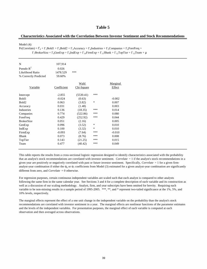
Model (4):

Pr(Correlate) = Г0 + Г1Bold1 + Г2Bold2 + Г3Accuracy + Г4Industries + Г5Companies + Г6ForeFreq +

Г7BrokerSize + Г8GenExp + Г9IndExp + Г10FirmExp + Г11IBank + Г12TopTier + Г13Team + μ

N 107,914

Pseudo R2

0.026

Likelihood Ratio 1478.529 ***

% Correctly Predicted 59.60%

Variable Coefficient

Wald

Chi-Square

Marginal

Effect

Intercept -2.855 (5530.41) ***

Bold1 -0.024 (0.63) -0.002

Bold2 0.063 (3.82) * 0.007

Accuracy 0.031 (1.48) 0.003

Industries 0.136 (18.35) *** 0.014

Companies 0.774 (522.86) *** 0.080

ForeFreq 0.429 (252.92) *** 0.044

BrokerSize 0.051 (2.16) 0.005

GenExp 0.096 (3.52) * 0.010

IndExp 0.100 (3.32) * 0.010

FirmExp -0.093 (7.64) *** -0.010

IBank 0.073 (8.76) *** 0.008

TopTier 0.143 (21.25) *** 0.015

Team 0.477 (40.42) *** 0.049

The marginal effects represent the effect of a one unit change in the independent variable on the probability than the analyst's stock

recommendations are correlated with investor sentiment in a year. The marginal effects are nonlinear functions of the parameter estimates

and the levels of the independent variables. For presentation purposes, the marginal effect of each variable is computed at each

observation and then averaged across observations.

Characteristics Associated with the Correlation Between Investor Sentiment and Stock Recommendations

Table 5

This table reports the results from a cross-sectional logistic regression designed to identify characteristics associated with the probability

that an analyst's stock recommendations are correlated with investor sentiment. Correlate = 1 if the analyst's stock recommendations in a

given year are positively or negatively correlated with past or future investor sentiment. Specifically, Correlate = 1 for a given firm-

analyst-year combination if either the α6 or α7 coefficients from Model (3) estimated for a given analyst-year combination are significantly

different from zero, and Correlate = 0 otherwise.

For regression purposes, certain continuous independent variables are scaled such that each analyst is compared to other analysts

following the same firm in the same calendar year. See Sections 3 and 4 for a complete description of each variable and its construction as

well as a discussion of our scaling methodology. Analyst, firm, and year subscripts have been omitted for brevity. Requiring each

variable to be non-missing results in a sample period of 1995-2005. ***, **, and * represent two-tailed significance at the 1%, 5%, and

10% levels, respectively.

39

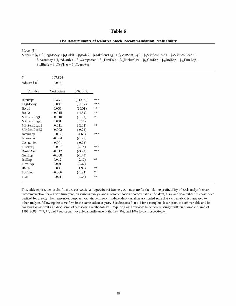
Model (5):

Money = β0 + β1LagMoney + β2Bold1 + β3Bold2 + β4MktSentLag1 + β5MktSentLag2 + β6MktSentLead1 + β7MktSentLead2 +

β8Accuracy + β9Industries + β10Companies + β11ForeFreq + β12BrokerSize + β13GenExp + β14IndExp + β15FirmExp +

β16IBank + β17TopTier + β18Team + ε

N 107,826

Adjusted R2

0.014

Variable Coefficient t-Statistic

Intercept 0.462 (113.09) ***

LagMoney 0.089 (30.17) ***

Bold1 0.063 (20.01) ***

Bold2 -0.015 (-4.59) ***

MktSentLag1 -0.010 (-1.88) *

MktSentLag2 0.001 (0.10)

MktSentLead1 -0.011 (-2.02) **

MktSentLead2 -0.002 (-0.28)

Accuracy 0.012 (4.63) ***

Industries -0.004 (-1.26)

Companies -0.001 (-0.22)

ForeFreq 0.012 (4.18) ***

BrokerSize -0.012 (-3.20) ***

GenExp -0.008 (-1.45)

IndExp 0.012 (2.10) **

FirmExp 0.001 (0.37)

IBank 0.005 (1.97) **

TopTier -0.006 (-1.84) *

Team 0.021 (2.33) **

The Determinants of Relative Stock Recommendation Profitability

Table 6

This table reports the results from a cross-sectional regression of Money , our measure for the relative profitability of each analyst's stock

recommendation for a given firm-year, on various analyst and recommendation characteristics. Analyst, firm, and year subscripts have been

omitted for brevity. For regression purposes, certain continuous independent variables are scaled such that each analyst is compared to

other analysts following the same firm in the same calendar year. See Sections 3 and 4 for a complete description of each variable and its

construction as well as a discussion of our scaling methodology. Requiring each variable to be non-missing results in a sample period of

1995-2005. ***, **, and * represent two-tailed significance at the 1%, 5%, and 10% levels, respectively.

40