This PDF is a selection from an out-of-print volume from the National Bureauof Economic Research

Volume Title: Annals of Economic and Social Measurement, Volume 3,number 4

Volume Author/Editor: Sanford V. Berg, editor

Volume Publisher: NBER

Volume URL: http://www.nber.org/books/aesm74-4

Publication Date: October 1974

Chapter Title: The Relative Efficiency of Instrumental Variables Estimatorsof Systems of Simultaneous Equations

Chapter Author: James M. Brundy, Dale W. Jorgenson

Chapter URL: http://www.nber.org/chapters/c10208

Chapter pages in book: (p. 679 - 700)

Annals of Ewn!Jmetric and Sodal Measuremem, 3/4, 1974

THE RELATIVE EFFICIENCY OF INSTRUMENTAL VARIABLESESTIMATORS OF SYSTEMS OF SIMULTANEOUS EQUATIONS

BY JAMES M. BRUNDY AND DALE W. JORGENSON

Consistent and effiCient estimaton of simultaneous equation.~ by the method of instrumenral I'l/riablesrequire an initial con.;istent estimator of the slructural form. Ins/rumental l'ariabie.~ estimators that areconsislent but not necessarily efficient can be employed for this purpose. The first objecti!"e Jj this paperis to measure the relative efficiency of alternUlil'e instrumental variables estimators proposed in theliterature. The secotui objective is to assess the sensitivity oflimited ;,iformation efficienr (LIVE) andfullinformatioll instrumenlal variables efficient (FIVE) estimators 10 the (hoice of an initial consistelltestimator.

1. INTRODUCTION

In previous papers (1971, 1973) we have provided a complete characterization ofthe class of consistent and efficient estimators of simultaneous equations by themethod of instrumental variables. Our characterization of consistent and efficientinstrumental variables estimators suggests two alternative ~pproaches to theestimation of simultaneous equations: 1

l. First estimate the reduced form by any consistent estimator. This approachunderlies the methods of two- and three-stage least squares.

2. First estimate the structural form of the model by any consistent estimator;then derive a consistent estimator of the redu-;ed (orm from the structuralform estimator. This approach underlies the methods of limited informa-tion efficient (LIVE) and full information instrumental variables efficient(FIVE) proposed in our earlier paper.

The approach to simultareous equations estimation based on consistentestimation of the structural form is easier to apply in practice. To obtain an initialconsistent estimator of the structural form the method of instrumental variablesprovides a promising approach. 2 A number of alternative instrumental variablesestimators have been proposed in the literature. Although these estimators differin efficiency and in computational difficulty, all of them are consistent. The firstobjective of this paper is to compare these estimators with regard to computationaldifficulty and to evaluate their relative efficiency.

In the following sections we first outline the simultaneous equations modelof econometrics. We then describe the statistical properties and computationalrequirements of alternative instrumental variables estimators. To evaluate therelative efficiency of the alternative estimators we compute estimates for KleinModel I.

The second objective of this paper is to assess the sensitivity of the LIVE andFIVE estimators to the choice of an initial consistent estimator of the structural

1 Ahistorical survey ofthese alternative approaches:s given in our earlier paper (1973), pp. 215--219.The LIVE and FIVE estimators were proposed, independently, by Dhrymes (1971).

2 The method of instnlmental variables was originated by Reiersel (1945) and Geary (1949). Adefinitive treatment of the method of instrumental variables for a single structural equation is givenby Sargan (1958).

679

form. We also consider the effect of iteration of the LIVE and FIVE estimators.On the basis ofour results we recommend the following approarh to the estimationof simultancous equations:

I. Estimate the strm;tural form by ordimuy least squares. This method isgenerally inconsistent.

2. Compute fitted values from the ordinary least squares estimators and usethese as instruments for the corresponding jointly dependent variables.This method is consistent but generally inefficient.

3. Compute fitted values for the second round estimator and proceed tocompute the LIVE or FIVE estimators proposed in our earlier paper.

The process described above can be truncated at the LIVE or FIVE estimators.Alternatively, the third step can be reiterated until the process converges. Thisiterative scheme coincides with Durbin's method for full information maximumlikelihood estimation ofsimultaneous equations in the case of the FIVE estimator. 3

The scheme coincides with Lyttkens' iterative instrumental variables method inthe case of the LIVE estimawr.4

2. THE SIMULTANEOUS EQUATIONS MODEl

We consider a simultaneous equations model with p equations: the structuralform of the model is denotcd:

(I) yr + XB = E,

with Y the matrix of observations on the p jointly dependent variables, X thematrix of n observations on the q predetermined variables, and E the matrix ofrandom errors; the matrices {r, B} of structural c.oefficients are unknown paramoeters to be estimated. The reduced form of the model may be written:

Y = xn -I- 1',

where the matrix n = - Br- 1 of reduced form coefficients is unknown andr = Er- I is a matrix of random errors.

Following the notation of Zellner and Theil (1962), we may denote theindividual structural equations by:

(2)where

z· = (y. X.]J J J '

(j = I, 2, ... , p),

in this notation Yj is a vector of observations on the j-th column of Y; the structuralcoefficient of this variable is normalized at unity; y. is a matrix of observations onthe other jointly dependent variables included in (he equation, Xj is a matrix of

J.S~ Durbin 0.963) and Malinvaud (1970~ pp. 686-687. The iterative process associated withDurbin s method IS Interpreted as an iterative application of the method of instrumental variables byHausman (1974) and Lytlkens (1971).

4 See Lyttkens (19'/0).

680

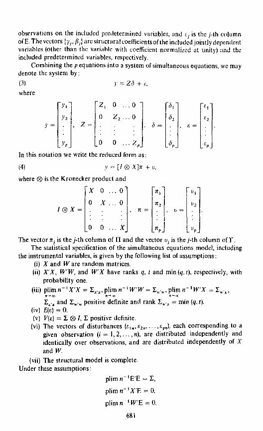
observations on the induded predetermined variables, <lnd I:j is the j-th columnof E. The vectors {y j' fi j: are structurall:oefficients of the included jointly dependentvariahles (other than the variahlr with coefficient normalized at unity) and theinduded predetermined variables, respectively.

Comhining the p equations into a system of simultaneous equations, we maydenote the system by:(3) )' :=; Z () + I:,

where

o ... 0

z=

l ~ 0 ... Zp

In this notation we write the reduced form as:

rJ1

lJ2

b = . , t: =

Jp

<: 2

(4) y = [I 0 X]rr + v,

where ® is the Kronecker product and

X 0 0' 1t 1 VI

0 X 0 1t2 V2I® X = , 1t= , v=

0 0 X 1tp L up

The vector lrj is the j-th column of n and the vector vj is the j-th column ofY.The statistical specification of the simultaneous equations model, including

the instrumental variables, is given by the following list of assumptions:(i) X and Ware random matrices.(ii) X' X, W'W, and W' X have ranks q, t and min (q, t), respectively, with

probability one.(iii) plim n- I X' X = I:x ' x ' plim n- I W'W = L\\""" plim n ~ I lV'X = L w'x ,

"-00 n~CL' n-"'x.

I:...x and 1:,.",., positive definite and rank L",..< = min (q, r).(iv) E(e) = O.(v) V(e) = 1: ® I, 1: positive definite.

(vi) The vectors of disturbances (c 1n , e211 , " . ,ern)' each corresponding to agiven observation (i = 1,2, ... ,11), are distributed independently andidentically over observations, and are distributed independently of Xand W.

(vii) The structural model is complete.Under these assumptions:

plim n-1E'E = 1:,

plim n- I X'E == 0,

plim n- I WE =: O.

681

Further, the vector ,,- 1/2[1 @ Xl I: is asymptotically normal with mean zao andvariance-covariance matrix L @ L,.,: the vector /1- 11 2

[1 ® W)'/: is asymptoticallynormal with mean zero and variance-covariance matrix 2: @ [ ....... 5

The most important properties of instrumental variables are that thesevariables are uncorrelated (asymptotically) with the errors E and that they arecorrelated (asymptotically) with the predetermined variables X. From the reducedform we can deduce that

plim /I-I W'Y = plim /I-I W'XO + plim /1"1 WT = [ ....,0,

so that under our assumptions the instrumental variables are correlated (asympto-tically) with the jointly dependent variables.

An additional assumption:

(viii) I: is N(O, I: ® I),

is essential for consideration of the problem of efficient estimation. Under thisassumption and the other assumptions we have made, the full information maxi·mum likelihood estimator attains the Cramer-Rao lower bound for the asymptoticvariance--eovariance matrix of (essentially) any consistent estimator of the struc-tural parameters. This bound, stated in terms of the asymptotic informationmatrix, depends on the likelihood function. Without an explicit likelihood function,such as that associated with a normal distribution of the errors, it is impossible todiscuss efficient estimation. Of course, the asymptotic distribution theory wedevelop for instrumental variables estimators is valid whether or not the errorsare normally distributed, provided that our other assumptions on the distributionof the errors are satisfied. While alternative estimators may be compared withregard to relative efficiency, no lower bound is available that would enable us tocharacterize any estimator as efficient in the class of consistent estimators.6

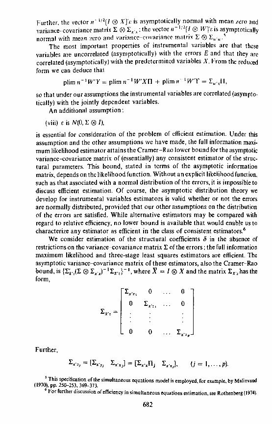
We consider estimation of the structural coefficients (j in the absence ofrestrictions on the variance--eovariance matrix L of the errors: the full informationmaximum likelihood and three-stage least squares estimators are efficient. Theasymptotic variance--eovariance matrix of these estimators, also the Cramer-Raobound, is {L~.JI: ® Lx·,r I Lx':} - I , where X = I ® X and the matrix Ix·:has theform,

Further,

o

o

oo

(j = I .... ,p).

5 This specification of the simultaneous eql:~tions model is employed. for example, by Malinvaud(1970), pp. 250-253,369-373.

6 For further discussion of efficiency in simultaneous equations estimation, see Rothenberg (1974~

682

In this expression X'X j is a submatrix of X'X and nj

is a submatrix of ncorresponding to the reduced form equations,

Yj = xn j + Y j •

We also consider estimation of the structural coefficients of a single equationbj , subject only to the identifying restrictions for that equation; the limitedinformation maximum likelihood and two-stage least squares estimators areefficient. The asymptotic variance-covariance matrix of these estimators, also theCramer-Rao bound, is UjjP;~'!JL;,~ Lx'x) - I, (j = 1,2, ...• pl. This completes ourdiscussion of the simultaneous equations model.

3. THE MHHOD OF INSTRUMENTAL VARIABLES

The method of instrumental variables for estimation of a single equation ina system of simultaneous equations is the following: We suppose that r

jjointly

dependent and Sj predetermined variables are included in the j-th equation andthat a subset or'tj = r j + Sj - I instrumental variables Wj is selected from theset of t instrumental variables W. The instrumental variables estimator d

jof b

jis

obtained by solving the equation:

Wi)'} = WjZjd j ,

obtaining,

(5) dj=(WiZrIWj.l'j.

Examples of instrumental variables are:I. The indirect least squares estimator,

dj = (X'Zr IX'Yj'

where t = P = r j + Sj - 1.2. The two-stage least squares estimator:

dj = {ZjX(X'X)-1 X'Zj} -IZjX(X'X)-1 X'Yj'

where W. = XIX'Xl- 1X'Z., the fitted values from a regression of the right-hand-side vari~bles in the equation Zj on the matrix of predetermined variables X.

We first observe that any instrumental variables estimator dj is consistentsince:

where:

plim (n- I WjZ) = [Lw;xI1j

is a matrix of constants and:

Lw,.•.J= Lw'.z·J"') r J

I· (-IW" 0p 1m n lj' = .Second, this estimator is asymptotically normal, since the vector n- I

/2 W~-€j is

asymptotically normal. Further, this distribution has expectation zero and. . . {~' ~-I '<' }-lvanance-<:ovanance matrIX Ujj ~Wj%/"wj'N/"wj:j .

683

The principal results of estimation theory for instrumental variables methodscan be embodied in two theorems presented here witholit proof. They are proved,and their implications discussed In detail, in our earlicr paper [1971 J.

Theorem A. Undcr the a:;silmptions given abo\'c, the cstimator

(6) dj = (WjZF Ill'jYj

of the parameters Jj of the equation (3) is asymptotically efficient if and onlyjf the matrix of instrumental variables Wj can be transformed by means of anonsingular matrix into a matrix that includes two subsets Wj = [Wjl , Wdwith the properties:

plim n- i Wjl X = njLx'x

I" -I W' X l'~p.!m n j2 = j"'x'x'

This theorem provides the necessary and sufficient conditions for consistent andefficient estimation of one equation from the model (I). The following theoremprovides the same conditions for an estimation of all equations taken together.

Theorem B. Under the assumptions given above, the estimator

(7)

of the parameters e5 in model (4) is asymptotically efficient if and only if the matrixof instrumental variables can be transformed by means of a nonsingular matrixinto a matrix with typical submatrix Wjj (W = :Wij}) that can be partitionedinto two subsets Wi; = [Wjjl ' Wij2] such that:

I· - I u:· X - ijn'~p 1m n Yf ijt - a j"'x'x'

I· -tW" X - ijl'~P 1m n ij2 - a j"'x'x'

where aij is the (i, j) element of the matrix I: - I.

With the above results available, alternative techniques for choosing It] andW can be considered.

Observe that for 2SLS and 3SLS, the instrumental variables for the includedjointly dependent variables in a particular equation may be written, in the notationused above,

(LIVE),

and

H~j' = s;jXfl j (FIVE).

The estimator fi j is a consistent estimator of the portion of the reduced formassociated with the j-th structural equations. Any consistent estimator of theseredueed form parameters can be used to generate estimators that are consistentand efficient. We have called estimators based upon a consistent estimator of thereduced form parameters Limited Information Instrumental Variables Efficient(LIVE) and Full Information Instrumental Variables Efficient (FIVE) estimators.

The instrumental variables used in LIVE and FIVE estimation are of theform xfi j , fi j a consistent estimator of the reduced form parameters n j' Because

684

model (I) is complete,

(8)and a consistent estimator 01 II is given by

(9)

where Band f are consistent estimators of the structural parameter matrices Band r of model (I).

Now the vectors Xfiare "fitted values" from a consistent estimator of thereduced form; they need not be developed from least squares, as in 2SLS or 3SLS,but can be obtained from the derived reduced form estimates (9). The "fitted val ues"can be determined without sOlving explicitly for the derived reduced form by thefollowing iterative algorithm:

Define the fitted values by

(10) Yr' 1 = - ¥.([ - I - l) - xD.

for any consistent estimators rand B, and iterate until ¥.+ 1 = Y,. + jl, II arbitrarilysmall. At that point,

(II)(; AA 1 ~

1,= -XBr- -jl=xn-/I.

The error in this iterative process (jl) must be zero if LIVE estimates obtainedfrom (II) are to be asymptotically efficient.

A. "True" Exogenous Insfrllrnental Variabies

In estimating the Liu quarterly model (1963) used to illustrate LIVE andFIVE estimation in our earlier paper (1971), we used as instruments those pre-determined variables which were not lagged values of jointly dependent variables.Instrumental variables do not need to be drawn from among the predeterminedvariables in the model, so long as the conditions stated above hold for the matrixof instrumental variables W.

In this method a set of instrumental variables Wi, which may d\lfer fromequation to equation, is chosen for consistentl) estimating the structural param-eters according to

dj = (WjZl-l Wj»

This preliminary consistent estimate provides the estimate of the reduced formfrom which instrumental variables for efficient estimation are obtained.

B. Repeated Least Squares ESlimarors

Theil [1958] and independently Basmann [1957] devised the method of two-stage least squares, in which the reduced form is estimated without constraint byordinary least squares, and the resulting fitted values used as regressors in struc-tural estimation. Zellner and Theii [1962] proposed the method of three-stage,least squares for estimating all equations simultaneously in a way equivalent tofull information maximum likelihood. Klein [1955] and Madansky [1964j demon-strated that the 2SLS and 3SLS estimators were instrumental variables estimators.

685

(12)

In the typical cconometric model, the number oi predetermin~d variables islarge in relation to the l1!1mbu (If nbscr\JllOm Further. predetermlncd variablcsarc often high Iy co!linear. ComputatIOn of ordinary lea~.' ~quares estImator of thereduced form is dlthcult. and inJu;J. lA-L0ni'::~ imr,,::'5~ib:.: wh.:n the number ofpredetermined variables ex<:ecd~the number of obscf\i:tions Computation of aderived reduced form estimator Circumvents thes::: dIfficultIes.

By analogy with two- and three-stage least squares. a number of estimatorshave been proposed whidl employ a multistage procedure. In such estimatorsregressions arc nm upon a subset of the predetermined variables. and the fittedvalues from these regressions substituted for the included jointly dependentvariables in second-stage regressions to estimate the SlrUClUral parameters. Theresulting estimator can be written

[f'r

d = )!) V'}·

,l\. j )

where f:. is the set of fitted \aiues from th.:: initial regressions:

(Di f, = l:d·,I'I<~ r.

In this expression J j is a set l)f predetermined \:iriables ,·hl)sen by any of themethods proposed abo..e.

Cooper (19721 employed arbitrary subsets (If the predetermined \"ariables ina rcpe3.ted least squares estimator. Fisher ll9651 proposed a method that took11 priori information in the IDl1del into a":":('unt in 5ele.:tmg subsets (If the pre-det~rmined y:.uiab!es thre-ugh a s~erwise regrns:CI!! prcx'X"\iure. A repeated leastsquares estimator based upon prin..:ipal components of the predetermined variableswas d~cribed by Klock and Mennes 119601 and discu~5oed by Arnemiya (1966).Another \ersion of the prin":lpal components estimator was applied by hans andKlein 119681 h.l the Wharton rnodei: this version has had \\idespread application.

Repeated Iea~i ~uares estimat0rs must be designed with ..:ace ifthe~' are to becl'nsistent or ~fficient. in our earlier pa~r. we Shl)WN that such e-stimaters areconsistent if they rNuee w instrumental variables estimators. Or if the initialregres.sil)ns happen to estimate the rele,ant rx"l111l)nS ef the reduced fonn con·~istentl~·. Repeated kast ~uarcs estlm..ilOrs are efficient l)nl~ if they pro\'ide":l)nsistent >'stimators l)f the rNu,,"ed fl)rm parameters.

The son· methl1d \\a~ prl1j:X)sed by fisher i J%:'l \\.b later Cl1m~ded by\ht..:hell Jnd Fi~her tI \)~Ot and was ;lppliN W the Br("-1ktn~s m(xiel by Miil;hell! 19'"'1 I. The meth,~ empll)ys the fl)!i,1\\ iug .1!~lmthm in ..:h,',)sing instraments fora jl.)intl\, dependent \ anahit :

1. Tl) c~ch predeurmineJ \;'!riJ.bk, .l.sslgn a \lXil'r \\ nh..1 number of elements,.'~u.ll W the rn.nimum ··l)rder··,)1 pre-.:ietermmN uriables app::aring inthe model. The mJ,\imurn ··,)!".ler"· l~ \jet~rmm~ in the Ct)UI'Se of furtherJ~\el,1pment l)i the 31~,)rithm .

... Order one is a..'i."igneJ ll.) c.a..:h rreJetermine-J ,.mable appoearing in the~u3til.)n defining the jl)intly dependent uriJ.1'k i"f \\hi..:h iostrutn(nts are

being developed. Order two is assigned to predetermined variablesappearing in equations defining the jointly dependent variables appearingin the first equation. Reappearance in the remaining equations of jointlydependent variables that have already been treated is ignored. Order threeis assigned to predetermined variables appearing in the equations definingjointly dependent variables appearing in the second equations. The proces;continues until all of the equations to be estimated as a simultaneous blockhave been used in accumulating the ordering vector.

3. At each occurrence of a predetermined variable in the previous procedure,an entry is made in the next unused location in the ordering vector for thatvariable. Entries from the equation defining the jointly dependent variablefor which instruments are sought are defined to have order one, and thefirst unused entry is assumed to have indefinite value.

4. The ordering vectors determine a lexicographic ordering on the predeter-mined variables. A variable with the ordering vector (1,3, (0) precedes onewith the vector (1,4,5, cx::-), and follows one with the ordering vector(I, 2, 3, (0). Frequently, two or more variables will have the same orderingvector; these variables are treated together as if they were a single variablefor purposes of the following analysis.

5. The significance of a variable or set of variables in explaining the varianceof the jointly dependent variable for which instruments are sought istested by a stepwise procedure. A regression is performed of the jointlydependent variable upon the largest possible number of variables or setsin the ordering for which moment matrices are nonsingular, omitting onlythe variables lowest in the lexicographic ordering, if any must be omitted.Then, the variable or set of variables appearing lowest in the ordering isdropped from the list ofregressors, and the resulting regression calculated.If the sum of squared residuals from the latter regression is SSEo, whilethat from the former set is SSE, the test statistic

F = SSEo/SSE [(n - q)/(n - qo)],

where q is the number of regressors in the former regression, and qo is thenumber in the latter, is distributed as F. A level of significance is chosen,and the hypothesis that the variable(s) omitted from the second regressionis significant is tested. If the variable is significant, it forms part of theinstrumental variables for the jointly dependent variable under study.The process is repeated until all variables or sets in the "structural order"have been tested. At each stage, significant variables (s) are retained in theset of regressors used for testing further sets.

If the resulting subset of the predetermined variables is denoted Xo, theMitchell-Fisher (1970) estimator is

(14)

where

2J = Xo(XoXo)-'XoZj'

687

This l'slilllalol is all illsllllll\('lIlal \H1I;thlrs I'slilll;llor, silll'l' il (';111 hl: wnih'lI

d, (7//1 I,?"I',

Till' rslilllallll lh~'ll IS tkllll~' nlllS;sll'lIl II IS !'Ilinl'nl onlv II ('\;"\01 I.\';'/,IS a('ollsisll'lIll'slilllllhH 01 II\(' pOll 1011 ollhl' redllced 101111 aSSlll'I;\I!'d wIth II\(' illrllhlt'djointly dl'pl'lHkll1 Villillhks,

n, 1'/'illl'il'lIl ('0/111'01/1'111,\ Il/sl/'t/lIIl'lI/fll 1'/II'i(/h1I',\ (P( 'II"

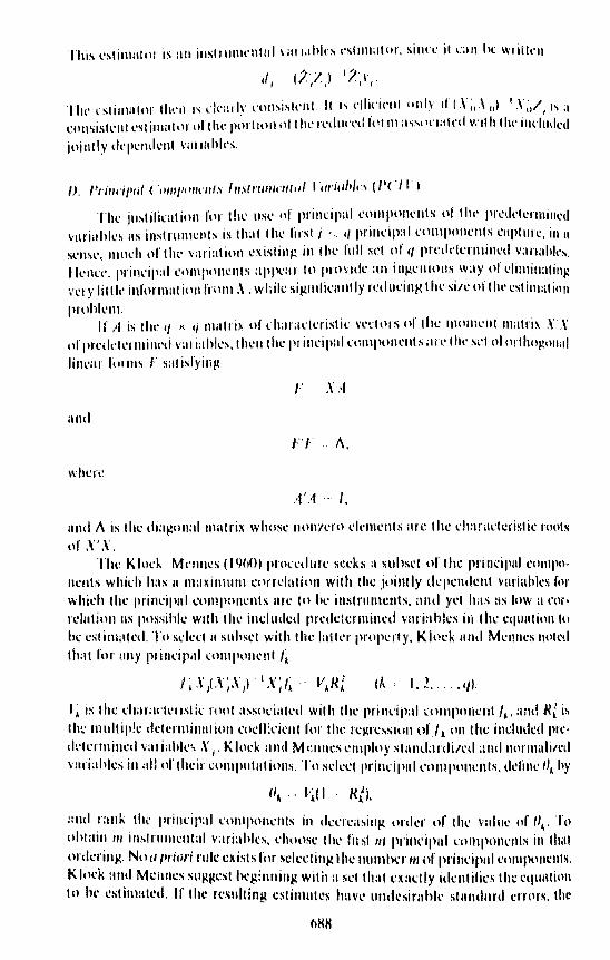
Thl' jllslilil'lilioll for Ihe lise of prilll:ipall'OIl1polll'nls ollhl' 11Il'dl'Il'rlllilll'dvllri.!hks liS insll'lllllcllls is Ihal lhl' lil'sl i . 1/ prillelpalcolIllllllll'lIl s l'upllll'c, ill II

Sl'IISl', 1I1l1l:h Ill' IIll' varialioll l'Xislillg ill Ihl' 1'1111 set of II prcdl'll'l'llIilll'd valiahb,I klll'I', prinl'ipall'lllIIl!ollcllb appl::1I 10 providl" all ill~l"lIiolls way of dilllin:lIillj:Vl'l'y lill II' inforllllll ion frolll ,\ , wIi ik signilil'a lilly r\.'d Ill'! nl{ Ihl' Sill' of II\(' csl illl:ll inllIll'Ilhklll,

If ;1 is thl' (/ )0, 'i malnx of charadl'rislie vl't'lnrs of Ihe 1I10llll'II1 lIlalrix ,\".\'of PI'l'dl'll'lllli IIl'd va l'iil hks, I IIl'lI Ihl' pI illl'i PillClllIIllllllCllI s "n: IhI' scI 01 orl hogoll;!1Iilll'ar !I II illS r salislyin~

and

,...r 1\,

lIlId 1\ is Ihe dia~oll:lllIllIlrix whllsl' 1I01l/l'IO dl'llIl'lIls lII'e IIll' dl:lr.ldcrblil' roolsof .\".\',

The KIOl'k MI'/lllcS II\)()Ol plOn'dme s.:cks a slIhscl of Ihe prindpllll'ollipn.IIl'lIls whidl Ius II III axiII III III corrdl!lioll wilh Ihe Joinlly (kpcndelll vllrillhks forwhich IIIl' prinl'iplIl \.'OI\lIHlIll~lIls llrl' III he inlilfllll1Cllts, lind yl'l h,IS as Iowa ('or,rclllliollllS p'lssihlc wllh Ihl' illdudcd prcdctcl'lIIillcd vlII'i:lhlcs iii lhl' equlIlionlohl'l'slil\l,lIed, To sdcl'IlI sllhsel wilh the lalln property, Kind llnd Mellncs nllledIhall'ol' !lily plinl'iIMIl'IlIIlP(lIlC!lll~

{, \' I \" \' I t \" f"I I' I' /' I • I I, I. >l, ' , , ,Ill,

I~ is Ih\.' dlill'''l'\l'l lsi il' 1'001 assol'iakll wilh Ihl' prilll'ipal UlIllpoJi,'1J1 fl , aild R; isIh~' lIlultiple dl'lcllllilllllilllll'odl:l'iclIllor II\I~ !'ej.tressioll of! 1011 the inl'llldcd pIC-ddl'llllilled v:lIiahks ,\, i' K lol'k lind M1:lIlieHlllploy slalllb rdi/l'll a lid 1I0rlllilhlCli\'llrlahlc~ ill ,,!lor Ihcil' UllllpUllllillilS, To lickCI prinl.'iplIll'IHlllllllll:lIls, delinl' til hy

(/1 ,I'll I Rfj.

::lId rallk Ih,' principal l'IlI\lPOIIl'lIls in dCl'l'l'i1sin~ Ilnkr of Ihl' VlI IIll' or (/1' TIlIlhillin III insfrlllllclIlal variahks, ehllllse IlIl' liist /I' pJ'illdpnl l'IllllpOl1l'nls ill lllll!orderillg, No (I f/l'ilit'/I'lllc ex isIs fill' sdel'lillJot Ihe lIumh..:r til ,If prilll'ipnll'IlJllponcnls,KlllCk alld M-:nnes sUllgcsl hcg:lllling wilh a sl'llhal nadly idelllilil'S Ihccquillion10 hc ~stilllall'd, H the l'(,'sllllillg elilillllll~1i haVl.' undcsirahk SllllldllJ'd cHors, Ihe

nU~ber of components is increased b.y using the next component in the ordering,until all components or all degrees of Ircedom are used without the standard errorsincreasing.

The Kloek and Mennes method results in a choice of "j for equation (13) thathils the form

v = [X P.]J J .r'

SO that the substitution estimator based upon the method reduces to an instrumen-tal variables method. As a result, the estimator always is consistent. but it will beefficient only in the mosl unlikely of circumstances.

The principal components estimator developed by Evans and Klein (1968) isa substitution estimator in which

This estimator will be consistent and efficient only if all principal components areused in Fj , in which case 2S'LS should be applied directly, or if the resulting estimateof the reduced form is consistent, a very unlikely event.

Taylor (1962) used principal components directly as instrumental variables,not in a repeated least squares estimator, in estimating the structural equations.While this method always is consistent, it cannot be efficient unless the conditionsof Theorem A, above, are fulfilled.

E. Iterated Instrumental Variables (1/ V)

The method of iterated instrumental variables was originated by Lyttkens(1970) and has been employed by Dutta and Lyttkens (1974). This method isinitiated by estimating the structural equations by ordinary least squares andderiving (inconsi3tent) estimates of the reduced form parameters for the purposeof computing reduced form fitted values. These fitted values then are used asinstruments for consistent estimation of the structural parameters, and the processis iterated until the parameter estimates cease to vary upon iteration. Clearly, onlyone additional iteration is required to produce LIVE estimates.

Durbin (1963) described a method for estimating the linear structural modelby full-information maximum likelihood that required that the following set ofnormal equations be solved by iteration:

[I ® W'Z][S-I @ I)c5 = [I ® WnS- t ® I)y.

In this expression, W is the set of instrumental variables obtained by fitting thederived reduced form estimates produced in the previous iteration and combiningthese with the predetermined variables appearing in the equations. Beginningfrom some consistent set of parameters, Wand b are calculated and the equationis solved for o. Iterating the process prod uces a new Wand a new lJ at each iteration,by using the implied estimator of the derived reduced form and the moment matrixof the residuals. At convergence, the estimator of b is the maximum-likelihoodestimator.

689

4. EMPIRICAL COMPARISON OF INSfRllME:-JTAL VARIABLFS ESTIMATORS

In view of the fact that only large-sample results are availahle about thestatistical properties of estimators for the linear simultancous equations model, itis of some interest to consider comparisons ;lInong consistent estimaiors of thecovariance matrices of the instrumental variables estimators disclIssed earlier. Ithas been shown above that a number of consistent estimators of the parametersexist which are not efficient. Comparisons ofconsistent estimators of the asymptoticcovariance matrices of these parameter estimators might provide some informationhelpful in selecting a method for choosing instrumental variables for consistentestimation. Intuitively, at least, it is appealing to argue that a method for choosinginstrumental variables which is estimated to have smaller asymptotic covarianceis superior to one having greater. Of greater importance are empirical evaluationsoftlie effect that choices of instrumental variables for the initial consistent estima-tion have upon the resulting LIVE and FrVE parameter estimates. If LIVE andFIVE are relatively insensitive to the initial choice of instrumental variables, thatchoice becomes of much less consequence.

Rothenberg (1947) presented measures of the gains in efficiency resulting fromtaking into account more a priori information. We employ similar measures incomparing the efficiency of IV, LIVE, and FIVE estimators. The results onminimum variance bounds given above imply that efficiency must increase as theestimation method moves from IV to LIVE to FIVE. Empirical estimation of theasymptotic covariance matrices of the estimators provides a means of evaluatingthe efficiency gain. While it is quite inexpensive to solve for reduced form fittedvalues when proceeding from IV to LIVE, LIVE estimates are at least twice asexpensive to produce as IV estimates. The increase in cost arises from the needto obtain reduced form fitted values and then to re-estimate the model, FIVEestimates are very substantially more expensive, since they involve not onlycomputation of the estimate of the structural covariance matrix ~, but alsoestimates of the coefficients. Preparation of these estimates requires inversionof a matrix whose order is the number of structural parameters. Even whenthis is possible, it is extremely expensive, since the computational effort involvedin most algorithms for inversion increases with the cube of the order of thematrix to be inverted. The value of incurring such a computational burdencan be weighed against the estimated increase in efficiency from proceedingfrom LIVE to FIVE.

Forecasting with an econometric mode! makes use of the reduced form of themodel. Therefore it is of interest to make the same inquiries about the estimatesof the reduced form that have just been described for the structural form:

1. What is the relative efficiency of alternative methods of developing reducedform estimates, using different choices of instrumental variables?

2. How sensitive are the reduced form parameter estimates derived from IV,LIVE, and FIVE estimates of the structural parameters to alternativechoices of the instrumental variables for initial IV estimation?

3. How significant is the gain in efficiency from proceeding from IV to LIVEto FIVE in terms of the efficiency of the reduced form estimators derivedflOm the structural estimator?

690

A. Klein Model J and Covariance Comparisons

We employ an annual model of the United States economy 1921-1941developed by Klein (1950), commonly referred to as Klein Model J, in measuringthe relative efficiency of alternative estimators of the structural and of the reducedform parameters. Kkin Model I has three behavioral equations and three identitie",.and is linear. It determines six jointly dependent variables from eight predeterminedvariables, including a dummy variable of constant unit value corresponding to theintercept in each behavioral equation. The model, as estimated by 2SLS, is givenin Table l. The parameter estimates given there are in al:cord with previous

TABLE I

KLEIN MODEL I 2SLS ESTIMATESAll Predetermined Vari<ibles as Inslruments

I. ConsumplionC = O.017P + O.216P_, + 0.8!flW + 16.6

(0.118) (0.107) (0.040) (1.32)R2 = 0.977 SE = 0.223

2. Inveslmenl1 = 0.150P + O.616P_ , - 0.158L, + 20.3

(0.173) (0.163) {O.0361 (7.54)R2 = 0.885 SE = 0.257

3. Privale Wagesw· = 0.439E + 0.147E_, + O.l30T + 1.50

(O.0361 (0.039) (O.029) (Ll5)R2 = 0.987 SE = 0.151

4. Corporate ProfitsP = C + I + G .- X - W

5. Wagesw= W· + W"~

6. Private ProduclE = X + P + w·Exogenous Variables:a. P_ 1 = Profils. lag Ib. K _, = CapiIal slock. lag Ic. E_, = Privale producl.lag Id. T = Timelrend. 1921. = -10

e. X = Indirecl laxesf. W·~ = Govemmenl wage billg. G = Governmenl expendiIures

estimates, for example, those reported by Rothenberg and Leenders (1964),although the computer program used for estimates treated 2SLS as a type ofinstrumental variables estimator.

For the purpose of quantitative comparisons of the relative efficiency ofalternative estimators, we employ consistent estimates of the covariance matricesof the alternative estimators, and compare these estimates against consistentestimates of the minimum variance bounds. The assumptions stated above implythat

(15) VlS = [Z;X(X'XrlX'Zirl(Z;X(X'X)-IX'Za

. (ZjX(X'xy-IX'Zjr1 'Sjj

691

is a consistent estimator of the minimum variance bound (9) for the covariancemairices of the estimators of the distinct equations which are efficient in the classof limited information estimators. The same assumptions, together with theassumptions abollt the properties of the instrumental variables, ensure that

'1IoF ) If _ rZ~II:(I".".u,:·) lU':L.J" l·lZ'.W{WW)-IW~W(W:w.)-IW'Z.]IV l" H, H, Yr, n, 'I '" I 'J) J ) J

. [Z'.W'W'.w.)-1 W'Z.J I. 5..- J j' ) J J) , I)

is a consistent estimator of the covariance matrix of the estimators of two distinctequations. when those estimators are consistent but not efticient. Because (15) isa consistent estimator of the minimum variance bound (MVB) for any consistentestimators of two distinct equations, (16) must differ from (15) by a positive semi-definite matrix, when the estimators for which (16) is the estimate of the covariancematrix are not efficient.

The MVB for estimators from the class of full information estimators (10) canbe estimated consistently, under the assumptions given above, by(17) JlJS = [S- 1 ® Z'X(X' X)-l X'Zr I.

The MVB for limited information estimators of all parameters, consideredtogether, differs from the MVB for full information estimators by a positive semi-definite matrix, and the same property holds for comparisons between a consistentestimator of the covariance matrix of the limited information estimators anI) theconsistent estimator of the covariance matrix for (efficient) full informationestimators (17).

Comparisons of the relative efficiency of alternative (derived) estimates of thereduced form depend upon the estimates of the covariilnce matrices for thestructural estimators just stated. The comparisons make use of the expression

(18)

for the covariance n'atrix of the derived reduced form, where ~ is the covariancematrix of the structural. estimator from which the reduced form estimates arederived. Expression (18) was obtained from Goldberger, Nagar, and Odeh (1961);a more direct derivation is available in Dhrymes (1970). The covariance matrix(18) is estimated consistently by replacing r, n, and ~ with consistent estimators.

The covariance matrix of the unconstrained reduced form (8) is estimatedconsis~ently by(19) VURF = ft ® (X'X)-l,

where ft is a consistent estimator of the reduced form covariance matrix n. Theestimator of the covariance matrix of the unconstrained reduced form (19) differsfrom any consistent estimator of the derived reduced form {I 8) by a positive semi-definite matrix.

Whenever the covariance matrices of the structural and reduced forms Landn, or any of their elements, appear in this analysis, they must be replaced byconsistent estimators. These matrices are estimated consistently by the momentmatrices of the residuals from consistent estimates of the structural and reducedforms, respectively. Throughout the subseqltent analysis, r, n, and L are replaced

692

by the estimates developed from two-stage least squares, while Q is estimated fromthe moment matrix of the residuals from ordinary least squares estimation of thereduced form.

To reduce the covariance matrices which are being compared to scalarmeasures of efficiency, three functions of the covariance matrices have beencomputed: 1) the sum of the elements of a covariance matrix; 2) the trace of acovariance matrix; and 3) the determinant of the covariance matrix. Each of thesemeasures preserves the ranking of the matrices in terms of relative efficiency, thatis, if B1 is the covariance matrix of an estimator that is more efficient than one withcovariance Bo, then anyone of the measures has the property that M(Bol > M(B t ),

where M denotes the fact that the measures are functions of the elements of thecovariance matrices.

Table 2 contains the results of estimating Klein Model I consistently by thefour inefficient instrumental variables methods we have presented. The coefficientestimates are very similar to those prepared by two-stage least squares in Table 1.

TABLE 2KLEIN MODEL I. CONSISTENT STRl;CTURAL ESTIM ...TES BY INSTRUMENTAL VARIABLE

Equalion Coefficienls

Variables (Slandard Errors)

SOIV PCIV TEIV IIV

I. ConsllmplionConstanl 16.43 i6.62 16.05 16.9!

(1.35) (1.42) (1.34) (1.33)*Profils 0.0667 -0.0003 0.0611 -0.1499

(0.142) (0.165) (0.140) (0.134)Profils. Lag I 0.1790 0.2305 0.1650 0.3388

(0.124) (0.145) (0.122) (0.117)·Wages 0.8078 0.8100 0.8248 0.8214

(0.040) (0.040) (0.041) (0.041)

2. InveslmentCOnSlaJ'it 21.22 25.77 22.84 21.41

(7.73) (11.3) (9.49) (8.04)·Profils 0.1i97 -0.0281 0.0671 0.1136

(0.182) (0.325) (0.255) (0.195)Profils, Lag I 0.6421 0.7690 0.6874 0.6474

(0.169) (0.287) (0.229) (0.180)Capilal Stock,

-0.1694 -0.1629Lag I -0.162(' -0.1827(0.037) (0.053) (0.044) (0.038)

3. Private Wages1.351Conslanl. 1.571 1.846 !.686

(1.15) (1.15) (1.15) (1.15)·Privale Product 0.4253 0.3732 0.4035 0.4673

(0.036) (0.041) (0.039) (0.040)Private Produel,

Lag I 0.1594 0.2087 0.1801 0.1198(0.03'.» (0.043) (0.041) (0.042)

Time Trend 0.1337 0.1464 0.1390 0.1235(0.029) (0.030) (O.O29) (0.029)

• Indicales an endogenous variable.

693

The coefficients are relatively stable across alternative choices of instrumentalvariables, with the pelV estimates varying slightly more from the 2SLS estimatesthan the others.

Parameter estimates derived from the use ofeach of the methods of consistentstructural estimation to develop fitted values for us~ as instrumental variables inpreparing LIVE estimates are given in Table 3. As might be expected, the parameter

TABLE 3KLEIN MODEL I. STRUCTURAL PARAMETERS ESH\fATED IlY LI.\lITED INFORMATION EH"lClENr

INSTRUMENTAl. VARIABlF$ (LIVE) METHODS

Equation Coefficients

Variable (Standard Errorl

2SLS SOIV PCIV TEIV I1V

I. ConsumptionConstant 16.55 16.79 16.74 16.77 16.80

(1.32)• Profits 0.0173 -0.1182 -0.1097 -0.1153 -0.!156

(0.118)Profits, Lag I 0.2162 0.3133 0.3056 0.3105 0.3121

(0.107)'Wages 0.8102 0.8214 0.8222 0.8217 0.8205

(0.040)

2. InvestmentConstant 20.28 21.50 21.52 21.63 21.60

(7.541·Profits 0.1502 0.1105 0.1098 0.1062 0.1076

(0.1 731Profits, Lag 1 0.6159 0.6500 0.6506 0.6537 0.6527

(0.!63)Capital Stock.

Lag I -0.1578 -0.1633 -0.1634 -0.1639 -0.1638(0.036)

3. Private WagesConstant 1.500 1.552 1.607 1.571 1.601

(US)'Private Product 0.4389 0.4290 0.4186 0.4254 0.4197

(0.0361Private Product,

Lag I 0.1467 0.1561 0.1658 0.1593 0.1648(0.039)

Time trend 0.1304 0.1328 0.1353 0.1337 0.1351(0.029)

• Indicates an endogenous variableNote: All limited information instrumental variables efficient estimators have asymptotic variances

and covanances equal to those oftwo-slage least squares.

estimates for each of the LIVE estimates except 2SLS are very similar, and they donot vary slgmficantly from the 2SLS estimates. Thus, the choice of instrumentalvariables for LIVE does not make appreciable difference to the resulting coefficientestImates.

694

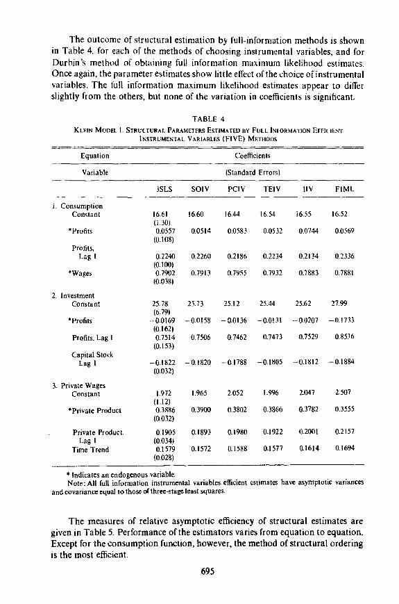
The outcome of structural estimation by full-information methods is shownin Table 4. for each of the methods of choosing inslrumental variables, and forDurbin'5 method of obtaining full information maximum likelihood cstimates.Once again, the parameter estimates show little effect of the choice of instrumentalvariables. The full information maximum likelihood estimates appear to differslightly from the others, but none of the variation in coefficients is significant.

TABLE 4KLEIN MODEl I. STRVtTURAI. PARAMETERS ESTIMATfO ElY FULLINWRMATION EFflUENT

INSTRUMENTAL VARIABLES (FIVE) METHODS

Equation Coefficients

Variable (Standard Errors)

3SLS SOIV PCIV TEIV ttV FIML

i. ConsumptionConstant 16.61 16.60 16.44 16.54 16.55 16.52

(UO)"Profits 0.0557 0.0514 0.0583 0.0532 0.0744 0.0569

W.W8)Profits,L~g I 0.2240 0.2260 0.2186 0.2234 0.2134 0.2336

(0.100)'Wages 0.7902 0.7913 0.7955 0.7932 0.7883 0.7881

(0.038)

2. InvestmentConstant 25.78 25.73 25.1 2 25.44 25.62 27.99

(6.79)"Profits --0.0169 -0.0.\58 -0.0136 -o.om --0.0207 -0.1733

(0.162)Profits. Lag I 0.7514 0.7506 0.7462 0.7473 0.7529 0.85.16

(0.1 53)Capital Stock

-0.1812 -0.1884Lag I -0.1822 -0.1820 -·0.1788 -0.1805(0.032)

3. Private WagesConstant 1.972 1.965 2.052 1.996 2.047 2.507

(1.12)

"Private Product 0.3886 0.3900 0.3802 0.3866 0.3782 0.3555(0.032)

Private Product. 0.1905 0.1893 0.1980 0.1922 1l.2001 0.2157Lag I (0.034)

Time Trend 0.1 579 0.1572 0.1588 0.1577 0.1614 0.1694(0.028)

" Indicates an endogenous variableNote: All futl information instrumental variables efficient estimates have asymptotic variances

and covariance equal to those of three-stage least squares.

The measures of relative asymptotic efficiency of structural estimates aregiven in Table 5. Performance of the estimators varies from equation to equation.Except for the consumption function, however, the method of structural orderingis the most efficient.

695

TABLE 5KUIN MODEl. 1. VARIANCE MEASURES "OR AI.HRNATlV!'. SlRUnURAl. ESTlMAlI';;

Equalion

M~asure

I. ConsumptionSumTraceGeneralizedVariance

2. InvestimentSumTraceGeneraljzedVariance

3. Private WagesSumTraceGeneralizedVariance

Entire ModelSumTraceGenerLllizedVariance

SOIV

1.7001.8460.479XIO"

58.8359.770.667XIO "

1.3061.3220.680XIO-"

64.6562.94

1.26X10- 29

!'elV

18922.0680.695XIO- ~

126.5128.9

2.13XIO- s

1.3181.3330.886XIO .1

137.5132.2

4.82XIO- 29

TEIV

1.69518390.474Xlo- s

88.6190.16

1.31XIO-"

1.3121.3270.781XIO- II

97.4593.32172X10- ~9

IlV

1.6651.8020.425XIO- g

617164.75

0.772XIO- s

1.3141.3300.831X10- II

70.7467.88

158X10 - 29

2SLS

1.6431.7720..124XIO- S

56.0756.95

0.607XIO" R

1.3051.3210.668XIO- I

'

62.6660.040.746\10- 29

3S1.S

1.5991.7250.239XIO- "

45.4746.26

0.476XIO" s

1.232l.2480.460XIO- Il

51.4249.180.220X/O- 29

The principal components method performed uniformly least well. Differencesamong the methods other than principal components (PCIV) are relatively small,in most cases. In view of the very considerable expense of developing SOIVestimates, UV would appear to be the method of choice for estimating KleinModel I by instrumental variables.

A gain in efficiency is achieved by employing limited information efficientestimators in place of any consistent but inefficient ones. Table 6 shows the gainin efficiency, based on the trace measure, from using 2SLS (or any other LIVEestimator) in place of the four consistent but inefficient methods. The efficiencygain is defined as the percentage increase from the trace of the covariance matrixof the LIVE estimator to the trace of the covariance matrices of the consistent but

TABLE 6EfFICIENCY GArN FROM USE OF MORE INFORMA nON STRUCTURAL ESTIMATES

(In Percen!. Based on Trace)

Estim~tjon Method Equation

IV to LIVE eNS INV w· MODEL

SOIV 4.2 4.9 0.0 4.8PCIV 16.7 126.3 0.9 120.2TElY 3.8 58.3 0.5 55.4IlV 1.7 13.7 07 12.4

LIVE 10 FIVE 2.7 29.8 5.9 22.1

696

inefficient estimators. Since SOIV estimat~sare relatively the most efficient of theconsistent but inefficient methods, the gain is least pronounced for this method.A further gain in efficiency is obtained by employing a full information estimatorin pla..:e of a limited information onc. The tracc measure used to construct Table 6makes it diilieul! to tell whether a greater gain is achieved by employing a fullinformation method instead of a limited information method or by using alimited information method in preference to a consistent but inefficient one. Thisresult is not in accord with results we reported earlier (1971) for the Liu modelusing generalized variance as the measure but agrees with the result reported forKlein Model I by Rothenberg (1974).

B. Comparison of Structural and Reduced Form Estimators

In this section, it is our objective to compare alternative estimators of thestructural and reduced form which employ different algorithms for selectinginstrumental variables, and which use different amounts of information. Whilewe have not reproduced the tables of reduced form parameter estimates which areanalogous to Tables 3, 4, and 5 above, the reduced form parameter estimates areno less stable than the structural estimates, with respect to choice of estimationmethod and choice of instrumental variables.

TABLE 7KLEIN MODEL I. EFFICIENCY MEASURF.5 FOR Rwucm FORM ESTIMATES

Equation E5timation Method

Measure SOIV pelv TEIV IIV 2SLS 3SLS OLSQ

I. ConsumptionTrace 85.70 108.59 85.12 75.88 67.98 63.49 829.85

2. InvestmentTrace 43.02 47.96 44.89 42.45 42.01 39.74 423.72

3. Private WagesTrace 52.00 62.00 54.55 50.78 48.26 45.63 576.47

4. Model·Trace 535.69 650.14 550.76 496.46 467.81 44i.91 5444.30

• In add~tion to measures for the three structural equations givcn above, the measure for theentire model includes the results for the three idcn tilies.

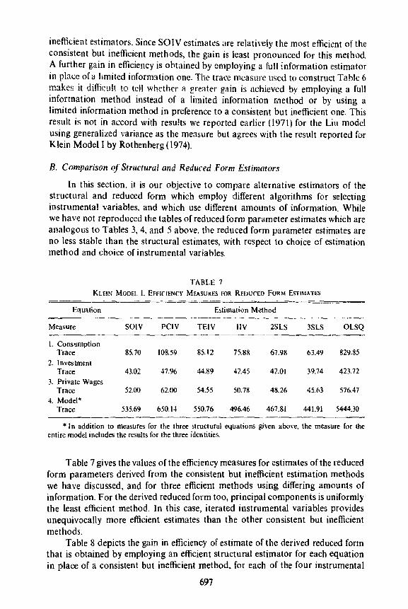
Table 7 gives the values of the efficiency measures for estimates of the reducedform parameters derived from the consistent but inefficient estimation methodswe have discussed, and for three efficient methods using differing amounts ofinformation. For the derived reduced form too, principal components is uniformlythe least efficient method. In this case, iterated instrumental variables providesunequivocally more efficient estimates than the other consistent but inefficientmethods.

Table 8 depicts the gain in efficiency of estimate of the derived reduced formthat is obtained by employing an efficient structural estimator for each equationin place of a consistent but inefficient method, for each of the four instrumental

697

TARLE REFFIClE"ICY GAIN FROM STRlIClLJRAL ESTlM" 1101" DrRIVED REIlUCW FORM

(In Percent. Based upon Trace)~ ---- .'--_-:::....-~":;: -,----'--~. --, .-=_ c--c:_,~, c_.=-

Etlua!ionEstimation Method ----~--_._---

eNS INY w· MODEl.

IV to LIVESOIV 26.1 2.4 7.7 14.5pelv 59.7 14.2 285 390TEIV 25.2 6.8 no 17.7I/V 11.6 I.l 5.2 6.1

LIVE to FIVE 7.1 5.7 5.8 5.9

variables methods we have described. The table also reflects the results of employ-ing FIVE instead of a LIVE estimator. The percentage gain from the use of LIVEmethods is substantial except for iterated instrumental variables, indicating thatfor Klein Model I the !IV method is nearly as efficient as LIVE. The gain fromusing structural information about the covariance matrix in obtaining derivedreduced form estimates is modest.

5. SUMMARY AND SUGGESTIONS FOR FURTHER RESEARCH

The results reported above lead to the following conclusions, on the basis ofalternative estimation of Klein Model I:

A. The most appealing method for consistent estimation of the linear struc-tural model is to begin with ordinary least squares applied to the structuralform. The fitted values of jointly dependent variables can be used asinstrumental variables to obtain a consistent estimator.

B. For efficient estimation the fitted values of the jointly dependent variablesfrom an initial consistent estimator should be lIsed as instruments inobtaining a LIVE estimator. The expense of computing FIVE estimatesmay well outweigh the benefits.

C. Choice of instrumental variables for obtaining a consistent estimatorappears to have little impact on the resulting LIVE or FIVE structural orreduced form parameter estimates. The implication is that the initialinstrumental variables should be chosen so as to minimize computationaldifficulty.

D. There appears to be no advantage and great computational difficultyassociated with iteration of the method of instrumental variables beyondliVE or FIVE estimators.

E. Where structural estimation is possible, it is to be preferred, as a means ofderiving an estimate of the reduced form, to unconstrained estimation ofthe reduced form.

The principal shortcoming of the research reported here is that the resultsapply with assurance only to one simple model. In the absence of general resultson the small sample properties of estimators for the linear simultaneousequations model, there is no way to avoid this difficulty. It would be ofconsiderablevalue to have available further results based on the application of our methods tolarger models.

698

The results could also be strengthened by using Monte Carlo techniques todevelop repeated samples for estimating the model. By repeating the analysis manytimes, based upon repeated samples from the same population, the degree ofdependence of coefficient stability and relative efficiem;y upon the data used toestimate the model could be investigated. Direct comparisons 01 the methodscould be made with respect to the error ofestimate, and some additional hypothesescould he tested. Such Monte Carlo experiments would be expensive and as opento criticism for dependence on a particular model as the results reported here.

The estimation techniques used here are not computationally dependent uponthe linearity of the model in the variables. Where nonlinearities can be expressedin terms of identities defining variables appearing in stochastic equations, theinstrumental variables methods can be applied. However, the statistical propertiesof such estimates are unknown; the results given above certainly do not apply.Since models used for practical purposes of economic analysis and forecastingmake extensive use of nonlinearities, the most pressing theoretical problem insimultaneous equations econometrics is to find estimators with desirable statisticalproperties that are suitable for nonlinear models.

The model we have used assumes that no autocorrelation is exhibited by anyof the errors on any equation. A useful generalization of the LIVE and FIVEmethods would be to modify them for the case of autocorrelated residuals. 7

Federal Reserlie Bank of Sall FranciscoHarvard University

REFERENCES

Amemiya. T. (1966). "On the Use of Principal Components of Independcnt Variables in Two-StageLeast-Squares Estimation," International Economic RevieK·. Vol. 7. No.3. September. pp. 283-303.

Basmann, R. (1957). "A Generalized Classical Method of Linear Estimation ofC;>efficients in a Struc-tural Equation." Econometrica. Vol. 25, No. I, January, pp. 77-83.

Brundy. J. and D. Jorgenson (1971), "Efficient Estimation ofSimultaneous Equations by InstrumentalVariables," Review of Economics and Stalisti,s, Vol. 53, No.3, August, pp. 207-224.

---and--(1973), "Consistent and Efficient Estimation ofSystemsofSimu]taneous Equations,"in P. Zarembka (ed.), Frontiers in Econometrics, New York. Academic Press, 1973. pp. 21S-244.

Cooper. R., (1972). '"The Predictive Perforrnan~e of Quarterly Econometric Models of the UnitedStates." in B. Hickman (ed.). Econometric Models of Cye/ical Behavior. Studies in Income andWealth, No. 36, New York, Columbia University Press, pp. 813-947.

Dhrymes, P. (1970), Econometrics: Statistical Foundations and Applicatior.s, New York, Harper &Row.

Durbin. J. (1963), "Maximum-Likelihood Estimation of the Parameters of a System of SimultaneousRegression Equations." unpublished manuscript.

Dutta, M. and E. Lyttkens (1974). "Iterative Instrumental Variables Method and Estimation ofa LargeSimultaneous System," unpublished manuscript.

Evans, M. and L. Klein (1963). The Wharton Econometric Forecasting Model, Philadelphia, EconomicForecasting Unit, Department of Economics, Wharton Schoo! of Finance and Commerce.

Fisher, F. (I 965a). "The Choice of Instrumental Variables in the Estimalion of Economy-WideEconometric Models." International Economic Review, Vol. 6, No.3. September, lip. 24S-274.

Fisher, F. (19Mb). "Dynamic Structure and Estimation in Economy-Wide Econometric Models:'in 1. Duesenberry. G. Fromm. l. Klein. and E. Kuh (eds.), The Bror;kings Quarterly EconometricModel of the United States, Chicago. Rand McNally, pp. 589-636.

7 Fair (1973) has proposed a modification of the LIVE and FIVE estimators that takes auto-correlation into account No analysis of the effkiency of the resulting estimators is currently available,

699

G~ilry. R. (1949). "Dd~Tmif1illion of I.in~'ar Relilllons iklWWl Sy~.tC:~1illIC P~rls of Varmblcs WithErrors of Obsl'fv;i1ion the Vananc<'S lif Whll'h ;lr~' lInknllwn. I: ("ol/lIlI/l'Iril"". Vol. 17. No IJanuary. pp. 30 58. ' ,

Goldhcrger. A" A. Nagl'f ilnd A Od~·h. (llJ611. "TIl<' Clll'ari:m,'c 1\Lttrix~s of R~t1l1l:~d-Forlll Coeffi.cients and of FOr~l';15ts fllr ;I Structur:ll El'lll1omc!rll' Mudd." !:"m//fiIlJClri"'i. Vol. 29. No. .;Ol'lober. pp. 55657.l .

Hallsman. J. (1974). "An lilslrumcntal Variable Approad: to Ful/·lnformation Estimators for Linearand Non-Linear Econon1l'tric Models," f.'nlllllll/ctrim. forthcoming.

Klein, 1.. (1950). Eco//omic HU(/lJllt;1I115 illthc Vlliteel SlIIteJ. /'):!/lWl. New York. John Wilty andSons. Inc.

_ (19~5). "On the Interprdation of Thcil'~ Mel~()d of Estimating Economic Relationships."J!(/crocc(/Il(/II/ico. Vol. 7. NO.3. December. pp. 14, 15.1.

Klock, T. and L. Mennes (1960). "Simultaneous Equaiions Estimation Based on Prindpal Componemsof Predl'lennined Variables,"~ f,'tI//(/l/Ictrim. Vol. 28. No. I. January. pp. 45 (;1.

Liu, T. C. (1963). "An Exploratory Quarterly Econ0melric M,x1e1 of Effective Demand Il1lhe Postwarl! S. Economv." Ecanomctrica. Vol. 31. No.3. July. pp. 301 J48.

Lytlkc~S. E (1970;. "Symml'lri( and Asymml'lric Estimation Methods." in E. Moshaek and H. Wold.II/!erdepelldem Sy.<t~IIlJ, Amsterdam. Norlh-Hol/and pp. 434459.

~~.__ (!971). "The Iterative Instrumental Variables Method aTld the Full Information Maximumlikelihood Method for Estima!ing Intcrdepcnd~'nt Systems." unpublished manUSl'fipL

Madansky. A. (1964). "O!! the Efficiency of Three-Sta~R' Least-Squares Estimation." EI'(J/wmmim.Vol. 32. No. 1-2, January April. pp. 51-56.

Mitchell. B. (!971), "Estimatlon of Large Econometrj~ Models by Principal Component ar.d Instru-mental Variable Melhods." RCl'ieli' I/f ECI/llt/min alld StGtistiC\·. Vol. 53. Nl'. 2. May. pp. 140-146.

Mitchell. B. and F. Fisher(1970). "The Choice of Instrumental Variables in the Estimation ofEcor.omy-Wide Econometric Models: Some Further Thoughts." [1lI('fl/I4I;w/II/ Ecollamic Rail"". Vol. II.No.2. June. pp. 226-234.

Reiersol. O. (1945). "Confidence Analysis by Means of Instrumental Sets of Vanables." Ark;\' forAfathematik. Astrfmomi 01'11 Frsik. Vol. 32.

Rothenberg. T. (1974). Efficient Estimatioll with A Priori IlIjim'llItioll. New Hawn. Yale UniwrsitvPress. .

Rothenberg. T. and C. Leenders (l9(4). "Efficient Estimation of Simultaneous Equation Systems:'Economeirica. Vol. 32. No. 1-2. January-April. pp. 57-76.

Sargan. J. (1968), "The Estimation of Economic Relationships Using InSll'umental Vanables.'·Econometrica. VoL 26, No.3, July. pp. 393--415.

Taylor. L. D. (1962). The Principal-Campanelll-Instrumental- Variable Approl/ch /II the EstimmiollofSrstems ofSimultalleolls Equations, unpublished. Ph.D. dissertation. Harvard Univcrsity.

Theil. H. (1971), "A Simple Modification of the Two-Slage Least-Squares Procedure for UndersizedSamples," Report 7107. Center for Mathematical Sludies in 8usines.~ and Economics. Universityof Chicago, February. 22 pp

Zel/ner. A. and H. Theil (1962). "Three-Stage Leas! Squares: Simultaneous Estimation of SimultaneousEquations," Econometrica. Vol. 30. No. 1. January. pp. 54-78.

700