August 1, 2004

The Relation among Human Capital, Productivity and Market Value:

Building Up from Micro Evidence

John M. Abowd (Cornell University, Census Bureau, CREST, NBER, and IZA),

John Haltiwanger (University of Maryland, Census Bureau, and NBER),

Ron Jarmin (Census Bureau),

Julia Lane (Urban Institute and Census Bureau),

Paul Lengermann (Federal Reserve Board),

Kristin McCue (Census Bureau),

Kevin McKinney (Census Bureau), and

Kristin Sandusky (Census Bureau)

*This paper was prepared for the NBER/CRIW conference on “Measuring Capital for the New Economy”

in Washington, D.C., in April 2002. The authors wish to acknowledge the substantial contributions of the

staff in the Longitudinal Employer-Household Dynamics (LEHD) Program at the U.S. Census Bureau. We

would also like to thank the participants at a pre-conference for helpful comments. This research is a part

of the U.S. Census Bureau’s LEHD Program, which is partially supported by National Science Foundation

Grant SES-9978093 to Cornell University (Cornell Institute for Social and Economic Research), the

National Institute on Aging, the U.S. Department of Labor (ETA), and the Alfred P. Sloan Foundation.

Any opinions, findings, and conclusions or recommendations expressed in this publication are those of the

authors and do not necessarily reflect the views of the U.S. Census Bureau or the National Science

Foundation. Confidential data from the LEHD Program were used in this paper. The U.S. Census Bureau

is preparing to support external researchers’ use of these data under a protocol to be released in the near

future.

Abstract

This paper investigates and evaluates the direct and indirect contribution of

human capital to business productivity and shareholder value. Human capital may

contribute in two ways: the specific knowledge of workers at businesses may directly

increase business performance, and a skilled workforce may also indirectly act as a

complement to improved technologies, business models, or organizational practices. We

examine links between the market value of the employing firm and newly created firm-

level measures of workforce human capital. The new measures of human capital come

from an integrated employer–employee database under development at the U.S. Census

Bureau. We link these data to firm-level financial information from Compustat, which

provides measures of market value and tangible assets. The combination of these two

sources permits examination of the links between human capital, productivity, and

market value. We find a substantial positive relation between human capital and market

value that is primarily related to employees’ previously unmeasured personal

characteristics that are captured by the new measures.

1

1. Introduction

The measurement of intangibles and human capital, important both for goods-

producing and for service-producing industries, has always been a difficult challenge for

the statistical system. The growth of the New Economy has made responding to this

challenge even more urgent: the need to understand how such inputs affect the value

chain of productivity, growth, and firm value now surpasses the need to measure the

contribution of bricks, mortar, and equipment. Yet, the changes that have brought the

New Economy into existence have also highlighted the need for improvements to

traditional measures of inputs and outputs (Haltiwanger and Jarmin, 2000), especially for

human capital. Finding new measures of human capital that are both quantifiable and

available for a sample large enough for use in official economic statistics is a formidable

challenge.

This paper uses newly available micro-level data from the U.S. Census Bureau on

both employers and employees to demonstrate a new approach to addressing this

challenge. We use new measures of human capital that directly capture the market

valuation of the portable component of skill, including the contribution of “observable”

and “unobservable” dimensions of skill. In principle, the measures go beyond indirect

proxies (such as measures of years of formal education) to quantify the value of

individual specific skills, such as innate ability, visual or spatial skills, non-algorithmic

reasoning, analytic or abstract decision-making, and “people skills” (Bresnahan,

Brynjolfsson, and Hitt, 2002). We present exploratory empirical results that relate the

new human capital measures to measures of labor productivity and market value.

An additional challenge has been to document the sources of firm-level

heterogeneity in productivity, growth, and value. One of the key findings of the literature

using micro-level data is that large differences exist across many dimensions of firm

2

inputs and outcomes. In particular, employers exhibit little uniformity in either the

methods they use to hire and fire workers or in the selection of types of workers they

employ. We therefore use measures of the dispersion of the firm-level human capital

distribution to capture relevant aspects of firm-level differences in organizational capital

and workplace practices.

We begin by describing the background, motivation, and underlying

specifications used in this chapter. Next, we describe the newly created data sources and

measures that underlie our study. The subsequent section provides an exposition of the

measurement of human capital that is made possible by the new Census data. We present

exploratory empirical results that relate our new human capital measures to measures of

firm performance including labor productivity and market value. The final section

concludes the paper.

2. Background, Motivation, and Specifications

The wide-ranging literature on human capital and intangibles is impossible to

summarize here. We can, however, provide a brief background to provide some

perspective on our approach. We begin with a discussion of our methodology for

measuring human capital and then consider the role of human capital at the firm level by

focusing on its potential relation to productivity, market value, and tangible and

intangible assets.

a) Human capital: conceptual and measurement issues

The importance of human capital in accounting for observed differences in wages

and productivity has a very long history in economics. Becker (1964) and many others

helped the profession define the components of human capital, and the contribution of

human capital to productivity has been intensively and exhaustively studied (e.g.,

Jorgenson, Gollup, and Fraumeni, 1987—hereafter, JGF). Clearly, we stand on the

shoulders of these researchers, but our approach differs in key ways that depend critically

3

on the availability of data. In particular, our conceptual and measurement approach

depends not only on the availability of longitudinal, matched employer–employee data

but the availability of universe files of all workers and firms.

The starting point for our approach has been well documented and investigated in

papers by Abowd, Kramarz, and Margolis (1999—hereafter, AKM) and Abowd,

Lengermann, and McKinney (2003—hereafter, ALM). In this paper, we exploit newly

developed measures of human capital that have emerged from this work and are part of a

new program at the Census Bureau called the Longitudinal Employer-Household

Dynamics (LEHD) Program. These and related papers emphasize a point that has long

been known in the study of human capital—direct measurements of human capital are

very difficult. The standard approach is to take advantage of the “usual suspects,” for

example, education and experience, and to build proxies for human capital using such

measures. In the productivity literature referenced above, this approach has made

extensive use of household data. Using primarily the Current Population Survey (CPS),

JGF create detailed measures of human capital from person-level data in the United

States by exploiting wage differences across groups defined by gender, experience, and

education. They aggregate these measures by industry and at the total economy level.

Their work demonstrates the existence of an enormous stock of human capital in the U.S.

economy and shows that the stock and flows of this asset are vitally important for

understanding changes in labor productivity.

However, JGF (and subsequent related work including the Jorgenson, Ho, and

Stiroh paper in this volume) recognize that this approach has limitations. Clearly,

industry and economy-wide aggregates fail to capture the firm-level variation that is a

driving force in productivity growth. In addition, the existing data provide only a

relatively small set of observable characteristics of workers, thereby creating

measurement problems, and omit measures of unobservable skill and confounding firm

effects. Using a college degree as a measure of human capital, for example, fails to

4

capture differences in school quality and program of study (Aaronson and Sullivan,

2001). The large portion of wage variation that cannot be explained by these variables

highlights the important role of the unobserved component of skill in the measurement of

human capital, as has been emphasized in the recent literature on rising wage inequality

in the United States (see, e.g., Juhn, Murphy, and Pierce, 1993). Finally, earnings

measures include the returns to working with particular firms—for example, large, highly

unionized, or profitable entities—and there is sorting among workers and firms. For these

reasons, AKM note that the estimates of returns to measured and unobservable

components of human capital may be biased.

We will describe in detail the econometric and measurement approach in

subsequent sections, but we will review here the basic specification used by AKM and

ALM so that we can discuss the conceptual basis of our human capital measures. The

core statistical model is

ijttiitiijt xw εψβθ +++= ),J( (1)

The dependent variable is the log wage rate of individual i working for employer j at time

t, while the function J(i,t) indicates the employer of i at date t. The first component is a

time-invariant person effect, the second the contribution of time-varying observable

individual characteristics, the third the firm effect, and the fourth the statistical residual,

orthogonal to all other effects in the model. In what follows, we use the person effect, θ,

plus the experience component of xβ as the core measure of human capital, called “h”

(i.e., hit = θit + xitβ).1 We also exploit these components separately as they clearly

represent different dimensions of human capital or skill.

For current purposes, our approach has three conceptual and measurement

advantages over earlier approaches. First, because we have data on the universe of

workers and of firms, we can create both firm-based and industry-based measures of

human capital that include measures of dispersion as well as central tendencies. In

5

particular, the new data permit the measurement of h and its underlying components for

all workers. Further, because we can associate all of these workers with their employers,

we can consider the full distribution of human capital for each firm and industry.

Second, the measure of h includes a broader measure of skill—the market valuation of a

number of observable and unobservable components—and, as such, encompasses various

measures of skill, including education.2 Because it includes the person effect, which can

be thought of as the portable time-invariant component of a person’s wage, the measure

of h also captures the influence of unobservable components of skill. Third, because the

AKM approach controls for firm effects in estimating the person effects, our measure of

human capital does not reflect personnel policies of the firm that may alter the returns to

observable and unobservable dimensions of skill.

Our approach has some limitations. First, the estimation method provides person

effects and firm effects that are time invariant. Both theory and evidence suggests that

firm effects and the returns to different dimensions of skill may be time varying.

Permitting time variation in the person and firm effects (e.g., through estimating a mixed-

effects or Bayesian model) is an active area of research in the LEHD Program. For now,

our interpretation is that we have a time average of the relevant effects.

Second, the specification does not permit any interaction between the firm effects

and the person effects. The implicit assumption in this specification is that firms pay the

same premium (or discount) regardless of the type of worker. This, too, is an area for

future work, but in this case we have some evidence to support our assumption. For

example, Groshen (1991a and 1991b) finds that establishment wage differentials exist

across occupations within establishments. Groshen’s result has been updated and

confirmed by Lane, Salmon, and Spletzer (2002), who use recent data from the

Occupational Employment Statistics survey of the Bureau of Labor Statistics (BLS); they

find that firms that pay premiums to their accountants also pay premiums to their janitors.

6

Third, this specification does not permit any co-worker effects. Yet, Lengermann

(2002a) has shown that whom you work with matters, as well as who you are and for

whom you work

Despite these concerns, we regard this base specification as a significant advance

over the standard approach of measuring human capital via observable education and

experience, for the reasons discussed above. We explore many of these issues in what

follows. For example, in section 3, we report the characteristics of our human capital

measures and, along the way, compare our results to more traditional estimates of human

capital. For now, we proceed to a discussion of how and why human capital might matter

for productivity and market value.

b) Human capital, tangible assets, intangible assets, and productivity

The relation between output and inputs is summarized by the standard production

function approach. Explicit recognition of human capital and intangibles augments this

function in the following specification of an intensive production function:

),,( jtIjt

Tjtjjt HKKFy = (2)

where yjt is output per worker for firm j at time t, TjtK is tangible physical capital per

worker, IjtK is intangible capital per worker, and Hjt represents measures of the

distribution of human capital of the workers at the firm.3

One of the conceptual issues that arises naturally in this setting is the possibility

that various features of the within-firm distribution of human capital differentiate firms

and are related to productivity. Consequently, studying the entire within-firm distribution

of skill rather than only the mean is justified by a number of theoretical underpinnings.

The relation between skill and productivity at the individual level might be nonlinear.

For example, empirical results support the widely held view that, for the experience

7

dimension of skill, the earnings-experience profile for an individual worker is strictly

concave and thereby reflects an underlying productivity-experience profile that is

likewise concave. Some other dimensions of skill may, however, yield a convex

productivity-skill profile. For example, “superstar” managers (e.g., Bill Gates) may make

a disproportionate contribution to the firm’s productivity and value. A related idea is that

the relation between productivity and, say, innate ability at the individual level may be

strictly convex. For our purposes, any nonlinear relation between the productivity of a

worker and the worker’s skill implies that higher moments of the within-firm distribution

of human capital will account for some variation in productivity at the firm level. For

example, if the productivity-skill relation for, say, the dimension of experience, is strictly

concave for the individual, then firms with greater dispersion on that dimension will have

lower firm-level productivity, other things equal. In contrast, if the productivity-skill

relation for the individual worker is strictly convex, then firms with greater dispersion on

that dimension of skill will have higher firm-level productivity.

These examples suggest only a few of the reasons that higher moments of the

within-firm distribution of human capital might be related to differences in productivity

across firms. The models of Kremer and Maskin (1996) suggest that, in some production

environments, interaction effects arise across the skills of co-workers in the production

function. For example, if the co-worker interaction effect reflects complementarities

across skill groups at the firm, then a business with lower dispersion will be more

productive.

In the analysis that follows, we are not imposing enough structure to be able to

identify which of these alternative and interesting factors may be the reason that the

8

within-firm distribution of human capital matters for differences in productivity across

firms. Instead, we take an eclectic, exploratory approach and simply include various

measures of the within-firm distribution of human capital in our estimation of the relation

between productivity, market value, and human capital.

Besides the interesting issues about the role of the within-firm distribution of

human capital, unmeasured (i.e., omitted) tangible assets and intangible assets may also

complicate the empirical link between human capital and productivity. Any

complementarities that may exist between unmeasured assets (or poorly measured assets)

and human capital may be reflected in any estimated relation between productivity and

human capital. Moreover, the nature of intangible assets may be very closely connected

to how human capital is organized.

c) Defining and measuring intangibles

A major issue confronting the productivity literature is the problem of studying

the effects of intangible assets when those assets are not readily measurable. Thus,

although some argue that intangibles are the “major drivers of corporate value and

growth in most sectors” (Gu and Lev, 2001), the definition of intangibles varies widely,

from knowledge and intellectual assets (Gu and Lev, 2001); to human capital, intellectual

property, brainpower, and heart (Gore, 1997); to knowledge assets and innovation (Hall,

1998); to organizational structure (Brynjolfsson, Hitt, and Yang, 2002—hereafter, BHY).

Measures of these variables have been equally diverse and have included a residual

approach, inference, and direct measurement.

For example, although Gu and Lev conceptualize intangibles as knowledge assets

(new discoveries, brands, or organizational designs), they derive their measure of

intangibles as a residual, that is, as the driver of economic performance after accounting

9

for the contribution of physical and financial assets. In empirical terms, they identify the

core determinants of intangibles as research and development, advertising, information

technology, and a variety of human resource practices. In a series of papers, Hall uses

direct expenditures on research and development as well as patent information to proxy

for knowledge assets. BHY use survey data on the “allocation of various types of

decision making authority, the use of self-managing teams, and the breadth of job

responsibilities” (p. 15) to construct a composite variable that acts as a proxy for

organizational capital.

The results from using these measures suggest that intangibles vary considerably

across firms and sectors and that they are important in accounting for fluctuations in the

market. Gu and Lev, who use the broadest measure of intangibles, find that the level and

growth rate of intangibles vary substantially across industries. In particular, they find the

highest levels in insurance, drugs, and telecommunications; the lowest in trucking,

wholesale trade, and consulting. However, they find the highest growth rates in

consulting, machinery, and electronics industries; the lowest in retail trade, restaurants,

and primary metals. Gu and Lev also find that intangibles-driven earnings (by two

different measures) are much more highly correlated with stock market returns than are

other measures, notably the growth of operating cash flow and the growth of earnings.

BHY find that organizational structure has a large effect on market valuation: firms that

score one standard deviation higher than the mean on this measure have approximately

$500 million greater market value. Hall finds that, although research and development

accounts for a “reasonable fraction” of the variance of market value, the relation is not

stable, and a great deal of the variation is unexplained. Patents matter, according to Hall,

but less than research and development.

Empirical studies also suggest that failing to include intangibles is likely to

considerably bias estimates of the effects of tangibles on both market value and output.

Gu and Lev find that expenditures on capital, R&D, and technology acquisitions are all

10

highly correlated with intangible capital. Similarly, BHY find evidence for a strong

correlation between organizational structure and investment in information technology.

Although the connections are difficult to conceptualize and measure,

organizational capital is closely linked to the way workers are organized and, in turn, to

the apparently different human capital mixes across firms in the same industry. As

emphasized in the preceding section, knowledge of the entire distribution of human

capital within each firm allows us to quantify the relation between outcomes like

productivity, market value, and the organization of human capital.

d) The market value of a firm—tangible assets, intangible assets, and human

capital

The general approach to describing the market value of a firm, Vjt, in terms of its

tangible and intangible assets is well summarized, derived, and motivated in BHY and

can be written as

,....),( Ijt

Tjtjt KKVV = (3)

The market value of a firm is assumed to be an increasing function of the assets.4

Defining and measuring all of the terms in this relation are difficult, however. If the

market is characterized by strong efficiency, then, as Bond and Cummins (2000) point

out, the market value of a company will equal the replacement cost of its assets (in the

absence of adjustment costs and market power). From this perspective, one way of

measuring intangibles is a residual approach (see, e.g., Hall, 2001), because the residuals

will reflect the difference between the market value and observed assets. Alternatively,

direct measures of intangibles (e.g., organizational capital, as in BHY) can be included in

an econometric specification explaining market value. However, such a specification

potentially permits the coefficients on the various assets to reflect direct and indirect

effects. One interpretation of the BHY coefficients is that they are due to

complementarities with unmeasured intangibles. Thus, the coefficient on any measured

11

asset will reflect the correlation between the measured and unmeasured assets. Thus, as

BHY have found, the coefficient on information-technology capital in a linear

specification of equation (3) is larger than 1. BHY provide evidence that this reflects the

complementarity between market value and organizational capital.

Should the preceding considerations lead one to include human capital in the set

of variables in an econometric specification of the market value equation? In the absence

of complementarities, a basic view of the role of human capital might suggest that it is

not relevant for the market value of the firm. That is, if all human capital is general

human capital, and if it is fully compensated by the market, and if no correlation exists

between human capital and unmeasured tangible or intangible assets, then human capital

will not be reflected in market value.

Several factors may, however, require departures from these assumptions. First,

human capital may not be fully compensated in the market. Second, the chosen mix of

human capital may indeed be a key aspect of what is meant by “organizational capital.”

As discussed above, many factors may yield a relation between productivity and higher

moments of the within-firm distribution of human capital. Under this view, the average

level of human capital at the firm may not matter for market value, but the way that

human capital is organized (as measured by higher moments) may matter a great deal.

Finally, human capital (its average and other measures of the distribution) may be

complementary to unmeasured tangible and intangible assets in a sense analogous to the

arguments and findings of BHY. As such, human capital may be positively related to

market value because of measures of tangible or intangible assets that are omitted from

the specification.

e) Econometric and interpretation issues

The previous subsections provided an overview of our approach. We explore

newly created measures of human capital from longitudinal employer–employee data.

12

These measures, in principle, encompass traditional measures and moderate some of the

econometric difficulties. In what follows, we explore the relation of these measures to

productivity and market value at various levels of aggregation. The discussion above

suggests that a host of econometric issues could arise to complicate the estimation of any

productivity or market value equation. At the heart of these issues is the well-known

problem that tangible assets and intangible assets, including those involving some

measure of human capital, are endogenous. The observed measures for any given

econometric implementation of equations (2) and (3) may also be proxies for other

unobserved measures. Our specification assumes that firms have control over the level of

human capital that they choose, and so an additional empirical concern is the degree to

which firms are constrained in adjusting their workforce (as noted by Acemoglou, 2001,

among others). Work by Haltiwanger, Lane, and Spletzer (2001) notes the remarkable

degree of persistence in firms’ choice of workforce. However, this overall picture of

firm-level persistence suggests that these firm choices are quite deliberate. Firms have

ample opportunity to change the workforce—a great deal of empirical evidence shows

that firms churn workers through jobs at quite high rates and hence have abundant

opportunities to change their worker mix (see, for example, Burgess, Lane, and Stevens

2000).

In this paper, we focus on identifying economically and statistically significant

relations rather than attempting to establish causality or to pin down direct vs. indirect

effects.5 We include measures of tangible and intangible assets in relatively simple

specifications of productivity and market value equations. We recognize that our

coefficient estimates reflect both direct and indirect effects of the assets we measure. In

particular, the effect of human capital on productivity and market value may include both

direct and indirect components. However, by looking at the effect on both productivity

and market value, we hope to make some progress in understanding the role of human

capital on business outcomes. If the measures of human capital are capturing mostly

13

general human capital, for which the worker is fully compensated, and if such human

capital measures are not correlated with unmeasured intangibles (or other unmeasured

assets), then human capital is likely to have a positive effect on productivity (as AKM

found in France) and very little effect on market value (because firms are fully paying for

the human capital and thus generate no additional value from having higher human

capital). However, if measures of human capital (or some components or indices of our

human capital measures) are positively related to productivity and market value, then the

measures are presumably capturing, either directly or indirectly, some form of intangible

asset associated with human capital.

We recognize the importance in this context of distinguishing the direct from the

indirect effects of human capital. However, as noted above, our objective is to explore

the links between our new measures of human capital and productivity and market value

in a largely descriptive manner. We anticipate that identifying and quantifying the

respective direct and indirect roles of these new measures of human capital in this context

will be the subject of much research in the years to come.6

One other related issue of interpretation warrants mention. We are exploring the

relation between productivity and human capital measures on the one hand, and market

value and human capital measures on the other. These two relations capture very

different aspects of firm performance. First, as already noted, any productive input that is

fully compensated in the market may be related to productivity but unrelated to market

value. Second, productivity captures current activity, while market value reflects future

profits and associated anticipated value. Thus, the factors that affect current activity may

be very different from those affecting future profit streams. One might argue that some

factors inherently lead to a negative correlation between market value and current

productivity. For example, a business with a “new idea” carrying a high market value

may be actively expanding and investing in physical and human capital. Adjustment

costs may imply that such a firm exhibits low current productivity.

14

3. Data

The key measures for this project are human capital, physical capital,

productivity, and market value. The integrated employer–employee data allow us to

construct firm-specific measures of human capital. The data from the Economic

Censuses provide measures of output, employment, and other inputs to explore the

relation between (labor) productivity and human capital measures. The Compustat data

on publicly traded firms provide us with measures of output, employment, physical

capital, and market value at the firm level. In terms of matching, we first match our

employer–employee data to the Economic Census and other business-level data at

Census. We then match the Compustat data to the integrated employer–employee,

Economic Census, and related data.

Figure 3.1 provides a brief summary of the data resources used for this project,

but of necessity it vastly reduces the number and complexity of the links involved in

constructing the matched employer-employee data. The details of these linkages can be

found in the appendix. However, we provide summary information about the data and

matching in the next two subsections.

15

Figure 3.1 Summary of Data Sources

Nationwide for 1980sand 1990s.

Nationwide -availability of somemeasures variesacross sectors andyears. EconomicCensus Dataavailable in 1992-97.

By State: Currently have for several States (1990s).

Availability:

Financial Data: Market value, "Q," intangibles, R&D, advertising, Capital,Output, Employment

via FirmIdentifier

Employment,Payroll, Sales,Productivity, R&D,ComputerInvestment, Entry,Exit, etc

via EIN

Earnings, Age, Education, Race, etc

Key Variables:

Firm Establishment, EI,Firm

Individual, EI Statistical Unit(s):

Compustat LBD, EconomicCensuses, AnnualSurveys, ACES,RD-1

UI files, CPS, SIPP

Source:

Financial Data Links toBusiness DataLinks toDemographic Data

Data Set:

a) The integrated employer–employee data

We exploit new Census Bureau data that are part of the LEHD Program. These

data integrate information from state unemployment insurance records and economic and

demographic data from the Census Bureau in a manner that permits the construction of

longitudinal information on workforce composition at the firm level. The LEHD

Program permits direct linking of the Census Bureau's demographic surveys (household-

based instruments) with its economic censuses and surveys (business-based and business-

unit-based surveys).

16

The unemployment insurance (UI) wage records are discussed elsewhere (see

Burgess, Lane, and Stevens, 2000). The Employment Security Agency in each state

collects quarterly employment and earnings information to manage its unemployment

compensation program. These data enable us to construct quarterly longitudinal

information on employees. The advantages of the UI wage records are numerous. The

data are frequent, longitudinal, and potentially universal. The sample size is generous,

and reporting for many items is more accurate than that in survey-based data. The

advantage of having a universe as opposed to a sample is that the movements of

individuals among employers and the consequences for earnings can be tracked. In

addition, longitudinal data can be constructed with the employer as the unit of analysis.

The LEHD Program houses data from nine states that currently comprise 45 percent of

total U.S. employment: California, Florida, Illinois, Maryland, Minnesota, North

Carolina, Oregon, Pennsylvania, and Texas. In this paper, we use data from seven of

these states and provisional national weights to build our human capital measures. We

currently have the crosswalk between the UI files and the establishment-level and firm-

level data for six of the seven states. For this reason, we restrict our analysis of the

relation between productivity, market value, and human capital to data from this six-state

subset.7

Perhaps the main drawback of the UI wage data is the lack of even the most basic

demographic information on workers (Burgess, Lane, and Stevens 2000). Links to

Census Bureau data can overcome this problem in two ways: First, the individual can be

integrated with administrative data at the Census Bureau containing information such as

date of birth, place of birth, and gender for almost all the workers in the data. Second, as

discussed in the previous section, LEHD Program staff members have exploited the

longitudinal and universal nature of the dataset to estimate jointly fixed worker and firm

effects using the methodology described in detail in ALM and in Abowd, Creecy, and

Kramarz (2002).

17

c) The Economic Censuses and related business-level data

The Economic Censuses (conducted every five years) provide comprehensive

data on basic measures such as output, employment, and payroll for all of the

establishments in the United States. In addition, in certain sectors (such as

manufacturing) the Census asks more-detailed questions on other inputs (such as capital).

Our first goal is to create a matched dataset linking the human capital measures to

the Economic Census data. For the present work, we focus on the Economic Censuses in

1997. One issue that immediately arises is the appropriate and feasible level of

aggregation of business activity. Although the Economic Censuses are conducted at the

establishment level, the business-level identifiers on our human capital measures are at

the federal Employer Identification Number (EIN), two-digit Standard Industrial

Classification (SIC) code, and state level.8 Therefore, we aggregate the Economic

Census data to the level of the business-level identifiers so as to match them to the human

capital files.9 Our unit of observation is somewhere between an establishment and a firm,

but most of the observations in our analysis data are at the establishment level. For firms

with multiple establishments reporting under a single EIN in a single state, we aggregate

the establishment data to the two-digit SIC, state level. In what follows, we begin our

analysis of the relation between human capital and productivity using this “quasi-

establishment level" data. For this analysis, we have roughly 340,000 business units that

we can match to the Economic Censuses (in a universe of roughly 430,000 business units

at this level of aggregation from the UI files for the six states used in this analysis). Most

of the UI businesses that we cannot match to the Economic Censuses are beyond the

scope of the Economic Censuses (for example, agricultural businesses). We are also able

to accomplish essentially the same thing in non-Census years using the Census Business

Register, previously known as the Standard Statistical Establishment List (SSEL).

Although the information in the Business Register is limited, it does identify the

ownership structure of firms so that we can further aggregate to the enterprise or firm

18

level. The latter aggregation permits us to match enterprise-level data on human capital

to Compustat.

Because we are working with only six states, we are limited in our ability to

examine evidence for large companies that operate in multiple states. We use a threshold

rule (for example, 50 percent of employment in the company must be in these six states)

to restrict attention to companies for which we can measure human capital and firm

outcomes such as market value and productivity in a comparable fashion. In what

follows, we first aggregate our human capital estimates up to the firm level for all firms

in our six states (using the 50 percent rule as noted). The resulting sample contains

roughly 300,000 firms. We use this sample to investigate the relation between human

capital and productivity at the enterprise or firm level. We then restrict our attention to

Compustat firms, which reduces the sample substantially because only about 13,000

Compustat firms exist nation-wide. For this restricted sample, we again investigate the

relations between human capital and productivity and also investigate the relation

between human capital and market value.

4. Human Capital Estimates

The results of the human capital estimation are based on data for seven states for

the years 1986-2000 and use the specification in equation (1). Although the methodology

and estimates we use are discussed in detail in ALM, we provide here a brief summary of

some of the features of the human capital estimates before relating these new estimates to

productivity and market value.

19

Standard Component Deviation ln w x β θ α uη ψ εLog real annualized wage rate (ln w ) 0.881 1.000 0.224 0.468 0.451 0.212 0.484 0.402Time-varying personal characteristics (x β ) 0.691 0.224 1.000 -0.553 -0.575 -0.099 0.095 0.000Person effect (θ ) 0.835 0.468 -0.553 1.000 0.961 0.275 0.080 0.000 Unobserved part of person effect (α) 0.802 0.451 -0.575 0.961 1.000 0.000 0.045 0.000 Non-time-varying personal characteristics (uη) 0.229 0.212 -0.099 0.275 0.000 1.000 0.101 0.000Firm effect (ψ ) 0.362 0.484 0.095 0.080 0.045 0.101 1.000 0.000Residual (ε ) 0.354 0.402 0.000 0.000 0.000 0.000 0.000 1.000Notes: Based on 287,241,891 annual observations from 1986-2000 for 68,329,212 persons and 3,662,974 firms in seven states as described in the text. No single state contributed observations for all years.Sources: Authors' calculations using the LEHD Program data bases.

Correlation with:Table 4.1: Summary of Pooled Human Capital Wage Components

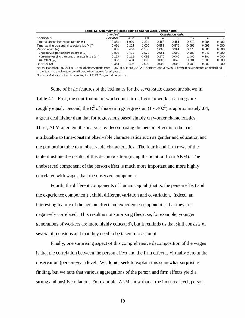
Some of basic features of the estimates for the seven-state dataset are shown in

Table 4.1. First, the contribution of worker and firm effects to worker earnings are

roughly equal. Second, the R2 of this earnings regression (1 - .4022) is approximately .84,

a great deal higher than that for regressions based simply on worker characteristics.

Third, ALM augment the analysis by decomposing the person effect into the part

attributable to time-constant observable characteristics such as gender and education and

the part attributable to unobservable characteristics. The fourth and fifth rows of the

table illustrate the results of this decomposition (using the notation from AKM). The

unobserved component of the person effect is much more important and more highly

correlated with wages than the observed component.

Fourth, the different components of human capital (that is, the person effect and

the experience component) exhibit different variation and covariation. Indeed, an

interesting feature of the person effect and experience component is that they are

negatively correlated. This result is not surprising (because, for example, younger

generations of workers are more highly educated), but it reminds us that skill consists of

several dimensions and that they need to be taken into account.

Finally, one surprising aspect of this comprehensive decomposition of the wages

is that the correlation between the person effect and the firm effect is virtually zero at the

observation (person-year) level. We do not seek to explain this somewhat surprising

finding, but we note that various aggregations of the person and firm effects yield a

strong and positive relation. For example, ALM show that at the industry level, person

20

and firm effects are positively related. Interestingly, Abowd, Haltiwanger, Lane, and

Sandusky (2001) show that at the firm level, person and firm effects are positively related

after controlling for output, local wage effects, and broad industry. These results by

industry and at the firm level are quite relevant here since they suggest systematic sorting

of workers across different firms and industries.

In the next subsections, we first provide some summary information about how

these new measures compare with the JGF-like measures of human capital. We also

describe the differences in the two components of the ALM measure of human capital—

experience and person effects—and how they vary across workers. Finally, we examine

the degree to which the human capital measures vary across firms and industries

a) A comparison of new and traditional measures of human capital

In principle, the JGF methodology can be applied equally well to the

measurement of both sectoral and aggregate labor quality, but in practice, the LEHD

approach permits more heterogeneity within and across industries. Lengermann (2002b)

has developed sectoral aggregates of human capital following the JGF approach and

compared them to LEHD estimates. Briefly, the JGF approach incorporates data from

the Censuses of Population, the Current Population Survey (CPS), and the National

Income and Product Accounts (NIPA). JGF base their labor quality indices on totals of

labor inputs cross-classified by sex, age, educational attainment, employment class, and

industry. We summarize the results of two different types of comparison here.

The first “direct” approach compares the JGF indices to sectoral labor quality

derived from industry averages of our human capital measure for the period 1995-98.

JGF formally define labor quality as the ratio of the total volume of labor to hours

worked, where volume is measured by a constant-quality index of labor quantity. The

LEHD measure of industry-average human capital follows essentially the same logic,

where the measure of labor volume is also based on a constant-quality human capital

21

measure and where total employment substitutes for total hours worked. Neither

approach is completely satisfactory. The LEHD data cannot measure hours worked. The

JGF constant-quality index of labor quality confounds firm heterogeneity with person

heterogeneity.

We compare the growth rates in the human capital indices over the period 1995-

98 using the LEHD-based and JGF approaches. The within-industry growth rates are

highly correlated—the employment-weighted average of the sectoral correlations is 0.79.

However, average growth for any given industry is much higher, and cross-industry

variation in those growth rates is much greater, in the LEHD measures than in the JGF

measures: the average growth rate for the LEHD measure over the four years is 0.04,

with a cross-industry standard deviation of 0.067, while the corresponding values for the

JGF measures are 0.014 and 0.001.

In what follows, we exploit cross-sectional variation (across firms) in their human

capital, whereas the JGF procedure focuses on generating growth rates of human capital

by industry. As such, the JGF measures are not well suited to examining within-year,

cross-industry variation. Thus, as a second “indirect” approach we approximate the JGF

labor quality indices with indices derived from predicted industry average wages

obtained by regressing wages on age, education, and sex using the CPS. For this

purpose, we use the same cells used by JGF. We show that the time series growth rates of

these indirect measures are highly correlated with the actual JGF measures (the

employment-weighted average correlation is 0.73). Thus, the CPS-based approach does a

reasonable job of approximating the more sophisticated JGF measures.

We compare the cross-industry variation in the CPS-based measures with the

same variation using the LEHD measures for the year 1998. The two measures are, in

principle, comparable because both rely on regression approaches that attempt to isolate

the component of wages due to individual characteristics. However, because LEHD data

permit individual contributions to wages to be distinguished from firm contributions, one

22

might not expect them to yield identical results. Workers sort nonrandomly into firms

based on their own characteristics—both observable and unobservable—and the

characteristics of firms. Furthermore, firm wage premiums—the firm effects in the wage

regression (1)—are not distributed uniformly across industries. These two facts imply

that a strong, positive correlation exists between person and firm heterogeneity at the

industry level (ALM)—a correlation that the JGF cell-based analysis cannot disentangle.

We plot the industry level aggregates for the CPS-based approach against the

industry level aggregates for the most inclusive measure of skill from the LEHD

approach (Figure 4.1). Although the levels are normalized differently, a great deal of

correlation clearly exists between the two measures—indeed, the correlation is 0.76.

However, somewhat more cross-industry variation exists in the LEHD-based measure

than in the CPS-based measure (the standard deviation of the former is 0.15, and that of

the latter is 0.13).

In summary, the LEHD-based measures by industry are closely related to those

derived by JGF or by a simpler but closely related CPS-based procedure. However,

LEHD-based measures generate greater average growth and more cross-sectional

variation both in growth rates across industries and in levels of human capital across

industries within a year.

Figure 4.1 Comparison of CPS and LEHD measures of Human Capital at the Industry Level

23

C P S B a s e d

LEHD Based -.5 0 .5

-.4

-.2

0

.2

1

2

3 4

5

7

89

10

11

12

13 1415

16

17

18

1920

21

22

2324

25

26

27

28

29

303132

33

34

35

36

37

38

39

40

41

42

43

44

b) The construction of new human capital measures

A major contribution of the LEHD approach is the richness of the new measures

of human capital, and these are fully discussed in ALM. Here, we explore some of the

key features of the new measures, particularly aggregated to the firm level. For this

purpose, we use three worker and firm traits to build measures of the human capital

resources available to firms: the person effect (θ), the overall labor market experience of

each worker captured by the experience component of βx (denoted βx in this section,

though it excludes the additional controls described in footnote 1), and the sum of these

two components (overall human capital, or h).

We describe the distribution of these measures in Figure 4.2. All three

components of the distribution obviously exhibit enormous variation across workers. The

shapes of the distributions of the alternative measures differ: The distribution of the

person effect is bell shaped and has thick tails and high variance; the distribution of

experience is less smooth; and the distribution of human capital (the sum of θ and βx ), is

24

roughly bell shaped and centered about zero and has much less mass at the tails than

either experience or θ. Underlying these relations is the negative correlation between

experience and person effects reported in Table 4.1.

Figure 4.2 Distribution of Human Capital across Workers

c) The construction of firm-level measures

Although the different worker-level measures of human capital provide a useful

context, the focus of this paper is on developing firm-level measures of human capital

and relating them to firm outcomes. The firm-level measures that we use are those

developed in ALM. They are based on kernel-density estimates of the within-firm

distribution of human capital. The details of the estimation of the kernel densities are

provided in ALM. Some restrictions on the sample that are necessitated by this approach

are discussed in detail in the appendix.

One key aspect of the variation across firms is driven by large variation in the

distribution of human capital across industries (Table 4.2). Finance, insurance, and real

estate (FIRE) and manufacturing are both high-human-capital industries. However, the

components of human capital vary across these industries: The FIRE industries have

high human capital especially because of having workers with high person effects, while

25

the high human capital of the manufacturing industries arises more through their having

workers with high experience effects.

Industry (SIC division)

Total Employment

Proportion of workers above the

overall median of h

Proportion of workers above the

overall median of θ

Proprtion of workers above the

overall median of x β

Agriculture 304,134 0.338 0.407 0.502Construction 1,366,022 0.510 0.465 0.556FIRE 1,382,730 0.531 0.591 0.439Manufacturing 3,365,954 0.539 0.473 0.560Mining 194,678 0.511 0.387 0.646PubAdmin 811,215 0.558 0.451 0.584Retail 3,537,787 0.383 0.542 0.388Services 7,856,442 0.493 0.520 0.468TCE 1,374,002 0.562 0.495 0.558Wholesale 1,626,221 0.567 0.529 0.540Notes: The sample is 1997 job-level UI data from 6 states. Includes all jobs held byworkers imputed to be full time at the end of the first quarter 1997.

Table 4.2: Summary Statistics on Human Capital by Industry (1997)

Human capital varies substantially across industries, but the variation across firms

within a given industry is enormous. We computed for each firm the share of workers

that are in the lowest quartile of the economy-wide distribution of human capital to obtain

the distribution of those shares across firms (Figure 4.3, left panel). We conducted the

same exercise for the share of workers at each firm that are in the upper quartile of the

distribution (Figure 4.3, right panel).

Figure 4.3 shows substantial differences both within and across industries. As is

consistent with the data in Table 4.2, many manufacturing and FIRE firms have low

shares of low-skill workers (lowest quartile), while retail trade has many firms with high

shares of low-skill workers. However, firms within an industry obviously vary

enormously in their shares of high- and low-skill workers. Apparently, different firms in

the same industry choose very different mixes of human capital; in the analysis that

follows, we will investigate whether this heterogeneity in human capital is related to

heterogeneity in productivity and market value.

26

Figure 4.3 – Between Firm Distributions of Human Capital, By Industry

5. The Relation between Productivity and Human Capital at the Micro Level

In this section, we explore the relation between our rich measures of

establishment-level human capital and establishment- and firm-level productivity,

controlling, as much as possible, for other relevant factors (capital intensity, for

example).10 For this purpose, we focus on the 1997 Economic Census. Our measure of

labor productivity is revenue per worker, the standard measure used in official BLS

productivity statistics for gross output per worker.11

An important goal is to determine which measures of the within-firm distribution

of human capital are relevant for understanding outcomes such as productivity and

market value. From a traditional viewpoint, we want to control for a measure of the

central tendency of the within-firm distribution of human capital. However, from the

perspective of considering nonlinearities and other factors related to the organization of

human capital at a business, we also want to explore additional measures of the within-

firm distribution of human capital. Our approach is necessarily exploratory since neither

theory nor earlier empirical research provides much practical guidance.

Accordingly, we explore the role of the following measures: (1) the fraction of

workers at the business whose human capital is above the economy-wide median, (2) the

fraction above the 75th percentile, (3) the fraction below the 25th percentile, and (4) the

interaction between—more specifically, the product of—measures 2 and 3. We consider

27

these four measures using the overall human capital measure h and also the separate

components of human capital (the person effect, θ, and the experience component, xβ).12

Moreover, we consider a range of specifications, some parsimonious (with only a small

number of summary human capital measures) as well as richer specifications with a

number of measures of the distribution included.

Table 5.1 presents the means and standard deviations of our human capital and

labor productivity measures for our overall sample and for the manufacturing businesses.

For the latter we can also measure capital intensity. The statistics reported in the table

are based on the employment-weighted distribution. In section 4, we discussed many of

the features of the human capital distribution across businesses. However, a few

additional points are worth making here (Table 5.1). First, businesses exhibit tremendous

heterogeneity in their mix of human capital as evidenced by the very large standard

deviations in the human capital measures. Second, manufacturing apparently has higher

labor productivity and workers with higher human capital (on both the person effect and

experience dimensions) than other sectors.

Variable Mean Std Dev Mean Std DevLog labor productivity 4.731 1.140 5.130 0.888Log capital intensity 4.230 1.201

Overall h = θ + x βFraction of employment above 50th percentile 0.480 0.215 0.538 0.225Fraction of employment above 75th percentile 0.237 0.176 0.267 0.185Fraction of employment below 25th percentile 0.266 0.172 0.208 0.169Interaction: fraction above 75th percentile with fraction below 25th percentile 0.042 0.025 0.035 0.022

Person effect (θ)Fraction of employment above 50th percentile 0.519 0.180 0.473 0.181Fraction of employment above 75th percentile 0.264 0.130 0.203 0.110Fraction of employment below 25th percentile 0.230 0.156 0.239 0.173Interaction: fraction above 75th percentile with fraction below 25th percentile 0.048 0.027 0.039 0.026

Experience component (xβ)Fraction of employment above 50th percentile 0.455 0.157 0.545 0.133Fraction of employment above 75th percentile 0.220 0.116 0.285 0.115Fraction of employment below 25th percentile 0.282 0.144 0.205 0.096Interaction: fraction above 75th percentile with fraction below 25th percentile 0.049 0.018 0.050 0.016

Number of observationsNote: The sample is 1997 data from 6 state UI-Based Firms (defined at the EIN 2-digit SIC level matched to EconomicCensus and Annual Survey of Manufactures data.

Table 5.1: Mean Values of Variables in Log Productivity RegressionsAll sectors Manufacturing

337,495 39,638

28

We made an exploratory analysis of the relation between log labor productivity

and our h measure of the distribution of human capital (Table 5.2) and an analysis using

the components of h separately (Table 5.3). In all cases, the results are based upon

employment-weighted regressions. All analyses included two-digit fixed industry

effects, which are highly significant. Moreover, the explanatory power of each set of

regressions is uniformly high; this result suggests that measures of human capital are,

either directly or indirectly, important sources of cross-sectional differences in

productivity. The fact that the explanatory power for the manufacturing sector

regressions is substantially less than that for all sectors is consistent with the notion that

human capital is more important for the service sector than manufacturing—and more

important for the “new” economy than the “old” economy.

(A) (B) (C) (D) (E) (F) (G)1.264 1.064 0.512

(0.007) (0.017) (0.017)

-0.017 0.268 0.430 0.1730.010 (0.012) (0.030) (0.027)

-1.875 -1.673 -1.143 -0.658(0.012) (0.012) (0.033) (0.031)

-3.032 -6.563 -3.870(0.063) (0.197) (0.187)

0.302 0.285(0.004) (0.003)

Number of observations 337,495 337,495 337,495 39,638 33,926 39,638 33,926R2 0.555 0.569 0.572 0.325 0.471 0.353 0.483Notes: The human capital measure is h = θ + x β . The estimation sample is UI-based establishments (defined at the EIN/2-digitSIC level) for six states matched to the 1997 Economic Census and Annual Survey of Manufactures data. Standard errors inparentheses. Other controls include 2-digit industry effects. Results are based on employment-weighted regressions.

Table 5.2: The Relation Between Labor Productivity and the Complete Human Capital Measure(Analysis level: Establisments; Dependent Variable: Log Labor Productivity)

All Sectors Manufacturing OnlyExplanatory Variable

Log capital intensity

Fraction of workers above 50th

percentile of human capital

Fraction of workers above 75th

percentile of human capital

Fraction of workers below 25th

percentile of human capital

Interaction of above 75th and below 25th percentiles

Businesses with a greater fraction of workers above the economy-wide median

human capital level are much more productive (Tables 5.2 and 5.3, column A). For the

overall human capital measure, a change in this fraction of one standard deviation is

associated with a change of 27 log points in labor productivity (Table 5.2). For the

person-effect measure (Table 5.3), a change of one standard deviation in the fraction of

29

high human capital workers is associated with a change of 25 log points in labor

productivity. For the experience component, a change of one standard deviation in the

fraction of high human capital workers is associated with a change of 23 log points in

labor productivity (Table 5.3). These effects are large, yet they reflect only a fraction of

the standard deviation in measured labor productivity across businesses (114 log points).

We also consider alternative measures of the distribution of human capital—

focusing on the fraction of workers with high human capital and those with low human

capital (Tables 5.2 and 5.3, columns B and C). Here the results are somewhat more

complicated to interpret but, in all of the results, a rightward shift in the distribution is

still associated with an increase in productivity. That is, if the share of workers in the

lower quartile is decreased a certain amount, and the share of workers in the upper

quartile is increased the same amount, then productivity increases; this result holds for

the overall h measure and for each of the components of the human capital measures.

However, asymmetric effects arise from changes in the upper tail and lower tail,

and the results are also sensitive to inclusion of an interaction effect. Moreover, the

nature of the asymmetries differs across components of human capital. The results for

the overall h measure show that changing the share of workers in the firm that are in the

lower tail of the human capital distribution has a disproportionate effect (Table 5.2,

column B). Somewhat surprisingly, the coefficient on the upper tail is negative but small

in absolute terms and relative to the coefficient on the lower quartile, and it is not

significant. The analogous column in Table 5.3 (column B) sheds further light on these

results and shows that different components of human capital act in different ways. In

particular, a disproportionate change arises from the upper tail of the person effect and

from the lower tail of the experience effect.

30

Explanatory Variable (A) (B) (C) (D) (E) (F) (G)1.400 1.240 0.670

(0.009) (0.024) (0.022)

1.990 1.700 2.060 1.480(0.015) (0.017) (0.050) (0.048)

-0.450 -0.920 -0.710 -0.299(0.010) (0.017) (0.043) (0.040)

2.830 3.110 1.941(0.078) (0.246) (0.230)

1.490 1.410 0.450(0.120) (0.032) (0.031)

0.200 0.760 0.540 0.135(0.020) (0.022) (0.062) (0.058)

-1.900 -1.560 -1.610 -0.713(0.017) (0.018) (0.081) (0.077)

-4.800 -7.020 -5.175(0.090) (0.328) (0.308)

0.310 0.298(0.003) (0.003)

Number of observations 337,495 337,495 337,495 39,638 33,926 39,638 33,926R2 0.547 0.564 0.568 0.315 0.471 0.360 0.496Notes: The human capital measure is h = θ + x β . The estimation sample is UI-based establishments (defined at the EIN/2-digitSIC level) for six states matched to the 1997 Economic Census and Annual Survey of Manufactures data. Standard errors inparentheses. Other controls include 2-digit industry effects. Results are based on employment-weighted regressions.

Log capital intensity

Fraction of workers above 50th percentile for x β

Fraction of workers above 75th percentile for x β

Fraction of workers below 25th percentile for x β

Interaction of above 75th and below 25th

percentiles for x β

Fraction of workers above 50th percentile for θ

Fraction of workers above 75th percentile for θ

Fraction of workers below 25th percentile for θ

Interaction of above 75th and below 25th

percentiles for θ

All Sectors

Table 5.3: The Relation Between Labor Productivity and Human Capital, Decomposed(Analysis level: Establisments; Dependent Variable: Log Labor Productivity)

Manufacturing Only

We have also devised an even richer specification in which we attempt to capture

the interaction between high-skill and low-skill workers (Tables 5.2 and 5.3, column C).

In this specification, we find that the linear terms have the expected signs: holding other

things constant, including the interaction effect, businesses with more workers in the top

quartile of the human capital distribution and fewer workers in the lowest such quartile

are more productive. However, the interaction effects are an important part of the effects

of interest. For overall h and the experience effects, we find that the interaction effect is

negative; whereas for the person effects, we find that the interaction effect is positive.

Putting the linear and interaction effects together reinforces the asymmetries we

have already noted. That is, for the person effects, we obtain a disproportionately large

change from an increase in the upper tail of the distribution, and the positive interaction

31

effect reinforces this asymmetry. This result can be seen by noting that the combined

linear and interaction effect for the person effect evaluated at the mean for the upper

quartile is 2.45, and the combined linear and interaction effect for the lower quartile is –

0.167. The magnitude of the implied variation in productivity is very asymmetric as

well. The combined effect implies that an increase of one standard deviation in the share

of workers in the highest quartile yields a change of 32 log points in productivity while

an increase of one standard deviation in the share of workers in the lowest quartile yields

a loss of 3 log points in productivity. The opposite pattern holds for the experience

effects. That is, the interaction effects reinforce the disproportionate change produced by

the lower tail of the distribution of the experience effect.

As discussed in section 2, the asymmetries in the effects of human capital on

productivity can be explained in a variety of ways. We cannot distinguish between

competing explanations, but our findings are consistent with the view that, at the worker

level, the relation between productivity and experience is concave, and the relation

between productivity and the person effect is convex. However, the results may also

reflect complementarities across co-workers that differ on different dimensions of skill.

Columns D through G of Tables 5.2 and 5.3 show results for the manufacturing

sector. Column D replicates column A but only for manufacturing. In column E, capital

intensity is an additional measure. For the most parsimonious specification, the results

for manufacturing are quite similar to those for the overall economy when we do not

control for capital intensity. Controlling for capital intensity does not change the

qualitative nature of the results, and although it reduces the magnitudes of the effects

substantially, they nonetheless remain very large. This aspect of the findings suggests

that human capital is complementary to physical capital. Thus, as we discussed in section

2, we need to recognize that our measures of human capital are capturing both direct and

indirect effects (where the latter stem in part from unobserved factors such as tangible

and intangible assets).

32

Columns F and G of Tables 5.2 and 5.3 present results for manufacturing using

the richer specification used in column C for all sectors—with and without a control for

capital intensity. Again, the results are quite similar to those for all sectors without

capital intensity. Once again, adding capital intensity reduces the magnitudes of most of

the effects from the human capital measures.

For manufacturing as a whole, capital–skill complementarity is clearly present.

Indeed, capital–skill complementarity seems to exist for all of the dimensions of skill we

are investigating. That is, the inclusion of capital intensity reduces the person effect, the

interaction effects, and the effect of the experience component.

How sensitive are these results to the level of aggregation? We address this issue

by aggregating establishment-level data from the 1997 Economic Censuses to the firm

level and estimating a set of similar regressions (Tables 5.4 and 5.5). The qualitative

results are very similar, and the most parsimonious specifications yield magnitudes that

are quite similar to the “establishment level" results in Tables 5.2 and 5.3. However, for

the more complex specifications, the magnitudes vary somewhat from the “establishment

level” results, especially when interaction effects are included. The differences in results

are most apparent for the manufacturing sector when we include interaction effects for

the overall h case and for the results on the experience component. Even in these cases,

the overall patterns are quite similar: the lower tail of the human capital distribution for

both h and experience at both the establishment level and the firm level produces

disproportionate effects.

33

(A) (B) (C) (D) (E) (F) (G)1.309 0.690 0.433

(0.007) (0.016) (0.015)

0.11 0.184 -0.194 -0.1890.011 (0.013) (0.031) (0.029)

-1.664 -1.621 -1.133 -0.786(0.011) (0.011) (0.028) (0.027)

-0.648 -0.889 -0.274(0.058) (0.166) (0.154)

0.256 0.248-(0.003) (0.003)

Number of observations 303,219 303,219 303,219 34,900 34,294 34,900 34,294R2 0.537 0.551 0.551 0.292 0.408 0.310 0.416Notes: The human capital measure is h = θ + x β . The estimation sample is Business Register-based firms (defined as those with atleast 50% of U.S. employment in the analysis states) for six states matched to the 1997 Economic Census and Annual Survey ofManufactures data. Standard errors in parentheses. Other controls include 2-digit SIC industry effects for the firm's primary industryand indicators for multi-location status and whether the firm had establishments in 1, 2 or 3+ 2-digit SIC categories. Results arebased on employment-weighted regressions.

Log capital intensity

Fraction of workers above 50th

percentile of human capital

Fraction of workers above 75th

percentile of human capital

Fraction of workers below 25th

percentile of human capital

Interaction of above 75th and below 25th percentiles

Table 5.4: The Relation Between Labor Productivity and the Complete Human Capital Measure(Analysis level: Firms; Dependent Variable: Log Labor Productivity)

Explanatory VariableAll Sectors Manufacturing Only

The differences that arise between the “establishment level” and firm-level results

may be due to increased measurement error of both the productivity and the human

capital measures at the firm level. Measuring productivity is more difficult at the firm

level than at the establishment level, especially for large, complex firms with many

establishments that cross industry boundaries. In a like manner, the human capital

measures are more complex at the firm level than at the establishment level because firms

with many establishments may differ in their distributions of human capital across

establishments. The latter situation is interesting in its own right, and we plan to explore

it in future work.

The results demonstrate powerfully that understanding differences in labor

productivity across businesses—particularly outside of manufacturing—involves

understanding differences in human capital across businesses. The close relationship

between labor productivity and human capital is clearly evidenced by the very large 2R

in the regressions, and the result obtains regardless of whether these are direct or indirect

effects and regardless of endogeneity issues. The results also clearly suggest that what

matters is not simply a measure of the central tendency of the human capital distribution.

34

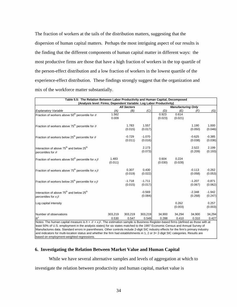
The fraction of workers at the tails of the distribution matters, suggesting that the

dispersion of human capital matters. Perhaps the most intriguing aspect of our results is

the finding that the different components of human capital matter in different ways: the

most productive firms are those that have a high fraction of workers in the top quartile of

the person-effect distribution and a low fraction of workers in the lowest quartile of the

experience-effect distribution. These findings strongly suggest that the organization and

mix of the workforce matter substantially.

Explanatory Variable (A) (B) (C) (D) (E) (F) (G)1.562 0.923 0.6140.009 (0.023) (0.021)

1.783 1.557 1.190 1.000(0.015) (0.017) (0.050) (0.046)

-0.729 -1.070 -0.625 -0.385(0.011) (0.016) (0.038) (0.036)

2.173 2.522 2.199(0.073) (0.209) (0.193)

1.483 0.604 0.224(0.011) (0.030) (0.028)

0.307 0.430 -0.113 -0.262(0.019) (0.022) (0.058) (0.053)

-1.718 -1.711 -1.207 -0.871(0.015) (0.017) (0.067) (0.062)

-0.569 -2.348 -1.942(0.084) (0.268) (0.247)

0.262 0.257(0.003) (0.003)

Number of observations 303,219 303,219 303,219 34,900 34,294 34,900 34,294R2 0.530 0.547 0.549 0.288 0.410 0.310 0.427Notes: The human capital measure is h = θ + x β . The estimation sample is Business Register-based firms (defined as those with atleast 50% of U.S. employment in the analysis states) for six states matched to the 1997 Economic Census and Annual Survey ofManufactures data. Standard errors in parentheses. Other controls include 2-digit SIC industry effects for the firm's primary industryand indicators for multi-location status and whether the firm had establishments in 1, 2 or 3+ 2-digit SIC categories. Results arebased on employment-weighted regressions.

Log capital intensity

Fraction of workers above 50th percentile for x β

Fraction of workers above 75th percentile for x β

Fraction of workers below 25th percentile for x β

Interaction of above 75th and below 25th

percentiles for x β

Fraction of workers above 50th percentile for θ

Fraction of workers above 75th percentile for θ

Fraction of workers below 25th percentile for θ

Interaction of above 75th and below 25th

percentiles for θ

Table 5.5: The Relation Between Labor Productivity and Human Capital, Decomposed(Analysis level: Firms; Dependent Variable: Log Labor Productivity)

All Sectors Manufacturing Only

6. Investigating the Relation Between Market Value and Human Capital

While we have several alternative samples and levels of aggregation at which to

investigate the relation between productivity and human capital, market value is

35

measured only at the firm level and only for publicly traded firms. Therefore, we are

constrained to using the relatively small matched Compustat sample (a detailed

discussion of the matched Compustat sample and variable definitions are in the

appendix). We report the means and standard deviations of this subset of observations

for 1996-98 (Table 6.1).13 Clearly these firms are more human capital intensive than the

full sample—the proportion of the workforce above the median economy-wide threshold

of skill (all measures) is greater, as is the proportion above the 75th percentile. The

proportion below the 25th percentile, by contrast, is smaller. However, all measures still

exhibit substantial heterogeneity: although the mean of each variable is different in the

two samples, the standard deviations are very similar.

Variable Mean Std DevEmployment 2,540 9,106Log market value 4.844 2.008Log capital 3.167 2.175Log other assets 3.814 2.086Multi-location indicator 0.780

Overall h = θ + x βFraction of employment above 50 th percentile 0.545 0.189Fraction of employment above 75 th percentile 0.291 0.163Fraction of employment below 25 th percentile 0.212 0.140Interaction: fraction above 75 th percentile with fraction below 25 th percentile 0.045 0.210

Person effect ( θ)Fraction of employment above 50 th percentile 0.560 0.179Fraction of employment above 75 th percentile 0.312 0.148Fraction of employment below 25 th percentile 0.207 0.138Interaction: fraction above 75 th percentile with fraction below 25 th percentile 0.049 0.023

Experience component (x β)Fraction of employment above 50 th percentile 0.460 0.147Fraction of employment above 75 th percentile 0.224 0.111Fraction of employment below 25 th percentile 0.264 0.126Interaction: fraction above 75 th percentile with fraction below 25 th percentile 0.048 0.015

Number of observations Note: Sample is pooled 1995-1998 data for Business Register-based firms, defined as those with at least 50% of U.S. employment in the six analysis states matched to Economic Census and Compustat data.

Table 6.1: Mean Values of Variables in Market Value Regressions All sectors

1,837

Tables 6.2 and 6.3 present the results of estimating equation (3), the (log) market

value regressions, using our two sets of human capital measures.14 In all specifications,

36

we find a strong, positive relation between (log) market value and physical and other

assets that is consistent with the theory and the empirical literature.15 The value added by

our analysis is that we can also measure human capital at the firm level. In our simplest

specification (Table 6.2, column A), a larger fraction of employees in the upper half of

the human capital distribution is associated with significantly greater market value. This

result is of interest because, if the compensation of highly skilled workers is

proportionate to their skill, and no correlation exists between unmeasured (tangible or

intangible) assets and human capital, market value should be unaffected once these other

variables have been controlled. Yet the estimated effect of human capital is quite large:

an increase of one standard deviation in the proportion of the workforce that is above

average is associated with a change of approximately 14 log points in market value (set

against a standard deviation of market value that is quite large—200 log points).

Explanatory Variable (A) (B) (C)0.732

(0.181)

0.579 0.554(0.269) (0.319)

-0.414 -0.451(0.313) (0.385)

0.343(1.785)

Log capital 0.421 0.422 0.422(0.026) (0.026) (0.026)

0.539 0.538 0.538(0.026) (0.026) (0.026)

Number of observations 1,837 1,837 1,837R2 0.851 0.851 0.851Notes: The human capital measure is h = θ + x β . Data were pooled for the years 1995-1998. The analysissample is firms in six states (defined as the firms with at least 50% of U.S. employment in the analysis states)matched to Economic Census and Compustat data. All regressions include year effects, 2-digit SIC effects for thefirm's primary industry, and indicators for multi-location status and whether the firm had establishments in 1, 2 or3+ 2-digit SIC categories. Standard errors in parentheses.

Table 6.2: The Relation Between Market Value and the Complete Human Capital Measure(Analysis level: Firm; Dependent Variable: Log Labor Productivity)

All Sectors

Log other assets

Fraction of workers above 50th percentile of human capital

Fraction of workers above 75th percentile of human capital

Fraction of workers below 25th percentile of human capital

Interaction of above 75th and below 25th percentiles

37

When we estimate more-complex specifications, we find that the effects of

different parts of the distribution of h on market value have some asymmetries that follow

patterns similar to those found for productivity. That is, we find that the upper tail of the

distribution of h has a disproportionately positive effect on market value and that the

interaction effect of the lower and upper tails is positive. The positive interaction effect

reinforces the asymmetry.

The decomposition of these results into person and experience effects is even

more striking, however. In particular, all of the positive effect on market value is due to

workers who have higher θ (person effects) (Table 6.3, column A). A striking result is

that, although both high-θ and highly experienced workers are more productive (Table

5.3), only the person effect is positively related to market value.

When we examine the more detailed specifications using the upper and lower tails

of the distributions of human capital, the results again show that high-person-effect firms

are higher-market-value firms; but, again, asymmetries appear in the effects of different

parts of the distribution. Column (B) of Table 6.3 shows that the upper quartile of the

person effect has a disproportionate impact on market value. Column (C) shows that the

interaction effect is positive. The disproportionate impact of the upper quartile found in

column (B) is also present in in column (C) , which can be seen by combining the linear

and interaction effects (evaluated at means). An increase in the upper quartile of the

person effect yields a combined effect (linear plus interaction) of 1.374, while an increase

in the lower quartile of the person effect yields a combined effect of –0.537.

38

Explanatory Variable (A) (B) (C)1.038

(0.242)

0.867 0.610(0.370) (0.385)

-0.455 -1.249(0.392) (0.543)

5.163(2.061)

0.001(0.292)

-0.964 -0.327(0.467) (0.520)

-0.682 -0.251(0.422) (0.491)

-4.776(2.501)

Log capital 0.424 0.428 0.428(0.026) (0.026) (0.026)

0.529 0.524 0.521(0.026) (0.026) (0.026)

Number of observations 1,837 1,837 1,837R2 0.854 0.855 0.857Notes: The human capital measure is h = θ + x β . Data were pooled for the years 1995-1998. The analysissample is firms in six states (defined as the firms with at least 50% of U.S. employment in the analysis states)matched to Economic Census and Compustat data. All regressions include year effects, 2-digit SIC effects for thefirm's primary industry, and indicators for multi-location status and whether the firm had establishments in 1, 2 or3+ 2-digit SIC categories. Standard errors in parentheses.

Fraction of workers above 75th percentile for θ

Fraction of workers below 25th percentile for θ

Interaction of above 75th and below 25th percentiles for θ

Fraction of workers above 50th percentile for xβ

(Analysis level: Firm; Dependent Variable: Log Labor Productivity)Table 6.3: The Relation Between Market Value and Human Capital, Decomposed

All Sectors

Fraction of workers above 50th percentile for θ

Fraction of workers above 75th percentile for xβ

Fraction of workers below 25th percentile for xβ

Interaction of above 75th and below 25th percentiles for xβ

Log other assets

We find it striking that the person effect is important in predicting market value.

Recall that the person effect is the component that includes “unobservable” components

of skill. Thus, one interpretation of these results is that value creation is highest for firms

that do a better job of attracting and retaining workers with dimensions of skill that are

difficult to observe. We also find it striking that the upper tail of the person effect

matters disproportionately. Those firms that have the highest share of the “best and the

brightest” workers (as measured by workers in the top quartile of the person effect) are

39

those with the highest market value. Again, more research is necessary to determine

whether these findings are due to the correlations between high-skill workers and

unmeasured assets (that is, omitted variables).

7. Summary and Concluding Remarks

Finding and quantifying new measures of human capital that could be introduced

into a firm-level production function is an important challenge for the federal statistical

system, particularly given the advent of the New Economy. This paper uses universe

micro-level data on both employers and employees to create new measures that begin to

address this challenge. Our new measures are closely related to those that have been

developed in the existing literature but the integration of the employer and employee data

permits a much richer measurement approach to human capital.

We document the substantial consistency between our new measures and earlier

measures pioneered by JGF (and subsequent closely related work). But we also extend

the previous work in a variety of ways. First, our human capital measures encompass the

traditional measures but also include effects not captured in traditional measures.

Second, our integrated data permit these human capital measures to vary within and

between firms in the same way that other inputs and outcomes can vary. Third, we

examine different aspects of human capital––pure skill, experience, and a summary

measure––and find marked differences in their distributions. We also use the richness of

the data, especially the firm-level distribution of human capital, to capture relevant

aspects of firm-level differences in organizational capital and workplace practices.

In the present analysis, we examine the relations between human capital,

productivity, and market value. Not surprisingly, for measures of human capital and

productivity, we find strong positive links in the micro data that differ according to the

component of human capital used. The most-skilled workers (in terms of the estimated

person effects) have a disproportionate positive impact on productivity, and the least-

40

skilled workers (in terms of the estimated experience effects) have a disproportionate

negative impact on productivity. We find that human capital is also related to market

value even after controlling for total physical assets.

Interestingly , the component of skill with factors that are “unobservable” (at least

to the econometrician) is most closely related to market value. At this stage of our

analysis, we are unable to distinguish the observable from the unobservable components

of skill. Future work might fruitfully explore this aspect of the analysis and results.

The new, micro-based measures of human capital incorporate unobservable

dimensions of worker’s skill. Our use of these measures to examine their role in

accounting for variation across firms is clearly exploratory. The strong empirical

relations that we have uncovered may reflect a variety of direct and indirect effects of

human capital.

41

References

Aaronson, Daniel, and Daniel Sullivan (2001). “Growth in Worker Quality.” Economic

Perspectives, 25 (4): pp. 53-74.

Abowd, John M. (1989). “The Effect of Wage Bargains on the Stock Market Value of the

Firm” American Economic Review, Volume 79(4) 774-800

Abowd, John M. (1990). “Does Performance-Based Managerial Compensation Affect

Corporate Performance” Industrial and Labor Relations Review, 43(3) 52S-73S.

Abowd, John M., Robert H. Creecy, and Francis Kramarz (2002). “Computing Person and

Firm Effects Using Linked Longitudinal Employer-Employee Data.”LEHD

Technical Paper No. TP-2002-06.

Abowd, John M., John Haltiwanger, Julia Lane, and Kristin Sandusky (2001). “Within and

Between Firm Changes in Human Capital, Technology, and Productivity.” LEHD

Technical Paper No. TP-2001-03.

Abowd, John M., Francis Kramarz, and David Margolis (1999). “High Wage Workers and

High Wage Firms.” Econometrica, pp. 251-334.

Abowd, John M., Paul Lengermann, and Kevin McKinney (2003). “The Measurement of

Human Capital in the U.S. Economy.” LEHD Technical Paper No. TP-2002-09.

42

Acemoglou, Daron (2001). “Technical Change, Inequality and the Labor Market.” Journal

of Economic Literature 40 (1) 7-72.

Becker, Gary S. (1964). Human Capital: A Theoretical and Empirical Analysis, with

Special Reference to Education. Columbia University Press.

Bond, Stephen R., and Jason G. Cummins (2000). “The Stock Market and Investment in the

New Economy: Some Tangible Facts and Intangible Fictions.” Brookings Papers

on Economic Activity (1): 61-124.

Bresnahan, Timothy F., Erik Brynjolfsson, and Lorin M. Hitt (2002). “Information

Technology, Workplace Organization and the Demand for Skilled Labor: Firm-

Level Evidence.” Quarterly Journal of Economics 117 (1): 339-376.

Brynjolfsson, Erik, Lorin M. Hitt, and Shinkyu Yang (2002). “Intangible Assets: How the

Interaction of Computers and Organizational Structure Affects Stock Market

Valuations.” Brookings Papers on Economic Activity: Macroeconomics (1): 137-

199.

Burgess, Simon, Julia Lane, and David Stevens (2000). “Job Flows, Worker Flows and

Churning.” Journal of Labor Economics, 18 (3): 473-502.

Foster, Lucia, John Haltiwanger, and C.J. Krizan (2001). “Aggregate Productivity Growth:

Lessons from Microeconomic Evidence.” in New Developments in Productivity

Analysis (eds. Charles Hulten, Edward Dean, and Michael Harper). University of

Chicago Press.

43

Gore, Al (1997). Speech at the Microsoft CEO Summit.

Groshen, Erica L. (1991a). “Five Reasons Why Wages Vary Among Employers.”

Industrial Relations 30 (3): 350-381.

Groshen, Erica L. (1991b). “Sources of Intra-Industry Wage Dispersion: How Much do

Employers Matter?” The Quarterly Journal of Economics 106 (3): 869-884.

Gu, Feng, and Baruch Lev (2001). “Markets in Intangibles: Patent Licensing.” Parker

Center for Investment Research Working Paper.

Hall, Bronwyn (1990). “The Manufacturing Sector Master File: 1959-1987.” NBER

Working Paper No. 3366.

Hall, Bronwyn (1998). "Innovation and Market Value." paper presented at the NIESR

Conference on Competitiveness and Productivity, London, England, February

1998. In Barrell, Ray, Geoffrey Mason, and Mary O'Mahoney (eds.),

Productivity, Innovation and Economic Performance, Cambridge: Cambridge

University Press, 2000.

Hall, Robert (2001). “Struggling to Understand the Stock Market.” (Richard T. Ely

Lecture) American Economic Review Papers and Proceedings 91 (2): 1-11.

44

Haltiwanger, John, and Ron Jarmin (2000). “Measuring the Digital Economy.” In E.

Byrnjolfsson and B. Kahin (eds.) Understanding the Digital Economy,

Cambridge: MIT Press.

Haltiwanger, John C., Julia I. Lane, and James R. Spletzer (2001). “Productivity

Differences Across Employers: The Role of Employer Size, Age, and Human

Capital.” Working Paper.

Jorgenson, Dale W., F. Gollop, and B.M. Fraumeni (1987). Productivity and US Economic

Growth. Harvard University Press, Cambridge, MA.

Juhn, Chinhui, Kevin M. Murphy, and Brooks Pierce (1993). "Wage Inequality and the

Rise in Returns to Skill." Journal of Political Economy 101 (3): 410-442.

Kremer, Michael, and Eric Maskin (1996). “Wage Inequality and Segregation by Skill,”

NBER Working Paper No. 5718.

Lane, Julia, Laurie Salmon, and James Spletzer (2002), “Establishment Wage

Differentials,” Mimeo, The Urban Institute.

Longitudinal Employer-Household Dynamics Program (2002). “Longitudinal Employer-

Household Dynamics Program: Employment Dynamics Estimates, Versions 2.2

and 2.3,” LEHD Technical Paper No. TP-2002-05.

45

Lengermann, Paul (2002a). “Is It Who You Are, Where You Work, or With Whom You

Work? Reassessing the Relationship Between Skill Segregation and Wage

Inequality” University of Maryland Ph.D. Thesis.

Lengermann, Paul (2002b). “Comparing New and Traditional Measures of Human

Capital,” Working paper.

46

Appendix

This section describes the construction of the data and key variables used for

analysis. Many of the steps involved in the formation of the data are part of the efforts at

the LEHD Project and the Center for Economic Studies (CES ) to develop data

infrastructure; these organizations have detailed the steps in a number of technical

documents. We provide here an overview of the data construction and refer to technical

documents as needed.

The process of constructing the data can be broken into two large segments. The

first segment is the formation of an “establishment level” file used in the productivity

analysis; the file contains human capital measures constructed from the LEHD database

and business traits from Economic Census micro data. The second segment is the

formation of a firm-level dataset that uses an aggregated version of the establishment file

matched to Compustat data for the years 1995-98.

Building the “establishment level” file

The process of building our approximation of an establishment-level file can be

summarized as follows: we use the LEHD database to estimate human capital measures

for each worker, and we use these measures along with a common economy-wide set of

thresholds to generate variables characterizing the distribution of human capital at each

business unit. Next, using data from the 1997 Economic Census micro data, we add in

measures of productivity for businesses in all sectors as well as capital intensity data for

manufacturing businesses.

The LEHD database links worker identifiers and demographic detail to employer

identifier variables. The construction of the LEHD database is described in detail in

LEHD Program (2002). We begin by using the database to compute human capital

measures for each worker using methods from AKM that are applied to the LEHD

database in the manner described in ALM. The time span of the data used to estimate the

47

person fixed effect varies across states; this paper uses human capital estimates drawn

from a seven state sample and uses matches of these estimates to establishment-level and

firm-level data for six states for the years 1995-98.

Using the worker-specific human capital measures from ALM, we create

variables summarizing the distribution of human capital at each business unit. We define

a business unit by Employer Identification Number (EIN), two-digit Standard Industrial

Classification (SIC) code, state, and year. This level of aggregation was selected because

it is the smallest that is common to both the LEHD database and the Economic Census

micro data. At this level of aggregation, most units are establishments, and thus, we refer

to this as an “establishment” file even though a multi-unit firm with multiple

establishments in the same two-digit SIC state cell will have data aggregated across those

establishments.

Although the LEHD data contain identifiers for all individuals employed by each

business during a given year, not all workers contribute to our characterization of the

human capital distribution at the establishment in that year. Rather, we identify workers

who are imputed to have worked full time at any job during the year and include from

that group only those who were working at the firm at the end of the first quarter of the

year.16 We restrict the set of jobs to those held by workers imputed to have worked full

time because we do not observe information on hours worked, yet we wish to separate

human capital effects from labor utilization effects. The timing restriction provides an

approximation of employment at a point in time and corresponds closely to point-in-time

employment as measured in the Economic Census, which collects employment for the

pay period that includes March 12.

48

All Full-time Jobs

All Full-time Jobs at End of First

Quarter

All Full-time Jobs at End of First

Quarter with 5+workers

(A) (B) (C)Number of establishments 1,391,839 1,078,877 429,529Number of jobs 40,967,355 21,829,227 20,156,292Fracttion of firms in agriculture 0.020 0.014 0.012Fraction of firms in mining 0.008 0.009 0.009Fraction of firms in construction 0.072 0.063 0.060Fraction of firms in manufacturing 0.125 0.154 0.162Fraction of firms in public administration 0.026 0.037 0.039Fraction of firms in FIRE 0.057 0.063 0.062Fraction of firms in retail trade 0.191 0.162 0.161Fraction of firms in services 0.380 0.360 0.356Fraction of firms in TCE 0.057 0.063 0.065Fraction of firms in wholesale trade 0.064 0.074 0.073Mean sales per employee 4.506 4.709 4.731Mean capital intensity 4.124 4.215 4.229Note: Statistics are employment weighted. Analysis samples are based on 1997 UI-basedestablishments for six states (defined as EIN/2-digit SIC units).

Table A.1: Summary Statistics for Alternative Samples

To evaluate the consequences of the restrictions on employment, we present

summary statistics for alternative samples (Table A.1). We further show descriptive

statistics for variables created from the establishment-level dataset that includes the full

set of possible jobs—that is, all jobs held by workers imputed to have worked full time at

any job in that year (column A). We also report the same set of measures with the added

point-in-time restriction (column B). When the point-in-time restriction is imposed, the

number of jobs falls nearly one-half (from almost 41 million jobs to about 22 million

jobs), but the number of establishment declined at a far lower rate, from about 1.4 million

to approximately 1.1 million. Establishments that are smaller and have higher worker

turnover are at higher risk of being eliminated by this restriction. A comparison of the

numbers across columns A and B suggests, however, that the two datasets vary only

slightly from each other in terms of industry composition. Specifically, column B has a

slightly higher share of manufacturing establishments (13 percent in column A; 15

percent in column B), a slightly lower share of retail (19 percent vs. 16 percent), and a

slightly lower share of services (38 percent vs. 36 percent). Businesses eliminated

49

through the point-in-time restriction appear to be less productive (lower sales per

employee) and, among manufacturers, less capital intensive, although these differences

are relatively small.

Many business units at this level of aggregation employ a small number of

workers. Our ability to characterize the distribution of human capital at small businesses

(here, those with fewer than five full-time employees) is limited because one worker can

make an enormous difference. Moreover, even for small to medium-size businesses, the

empirical distribution of human capital at a firm is quite noisy and potentially misleading.

For example, the firm may have some positive probability of having workers in a

particular percentile range but in fact have no workers in that range at a point in time.

For these practical as well as conceptual reasons, we generate measures of the within-

firm distributions based upon the kernel-density estimate (for h and for each of the

components) for each firm (see ALM for details).

The use of this method involves trade-offs, however. The method allows us to

measure the human capital at businesses more accurately, but the data requirements for

the estimation procedure prevent us from using the smallest of firms in our analysis.

Specifically, we generate a kernel-density estimate for each of the three human capital

measures at each business that has at least five full-time workers at the end of the first

quarter in a given year.

The size restriction eliminates less than 10 percent of jobs (about 1.6 million out

of about 22 million) (Table A.1, columns B and C).17 However, this restriction causes

the number of business units to decline more than 60 percent (from about 1.1 million to

less than 430,000). Summary statistics suggest, however, that although the firms lost

through this restriction are small, they are spread evenly throughout all sectors of the

economy and do not differ substantially in mean level of productivity or capital intensity. We use a common set of thresholds to construct the establishment-level skill

measures for the pooled distribution of all jobs held in all states currently in the LEHD

50

database by workers imputed to have worked full time at the end of the first quarter of

1997. These thresholds are the median, the 75th percentile, and the 25th percentile value of

each of the three human capital measures. We then calculate the cumulative density at

each business between each of the thresholds to generate the proportions above the

economy-wide median and economy-wide 75th percentile of h and the proportion below

the economy-wide 25th percentile of h. We construct similar measures for θ and xβ.

The mean value of each human capital measure is sensitive to the set of sample

restrictions imposed as well as to the method used to compute business-level skill (Table

A.2). Columns A through C correspond to columns A through C in Table A.1 in terms

of the restrictions imposed on the data. To generate the mean human capital measures

reported in each of these three columns, we use the same set of thresholds described

above along with the empirical distribution at each business unit rather than the smoothed

estimate. Column D presents summary statistics derived from the smoothed kernel-

density estimate of the distribution at each business. Thus, differing methods are used

on the same set of workers and firms to generate the means in columns C and D. In this

way, we are able to isolate the effect of each sample restriction as well as the effect of

using kernel-density estimates of the distribution of human capital at each business.

51

All Full-time Jobs

All Full-time Jobs at End of First

Quarter

All Full-time Jobs at End of First

Quarter with 5+workers

All Full-time Jobs at End of First

Quarter with 5+workers, Using

Kernel Density Estimates

(A) (B) (C) (D)Number of "Establishments" 1,391,839 1,078,877 429,529 429,529Number of Jobs 40,967,355 21,829,227 20,156,292 20,156,292Fraction of workers above 50th percentile for human capital 0.403 0.496 0.502 0.497Fraction of workers above 75th percentile for human capital 0.187 0.246 0.245 0.248Fraction of workers below 25th percentile for human capital 0.339 0.254 0.242 0.257Interaction of above 75th and below 25th percentiles for human capital

0.039 0.038 0.038 0.043Fraction of workers above 50th percentile for θ 0.507 0.511 0.520 0.513Fraction of workers above 75th percentile for θ 0.254 0.256 0.258 0.261Fraction of workers below 25th percentile for θ 0.253 0.245 0.232 0.236Interaction of above 75th and below 25th percentiles for θ 0.051 0.046 0.046 0.049Fraction of workers above 50th percentile for xβ 0.421 0.490 0.481 0.473Fraction of workers above 75th percentile for xβ 0.205 0.248 0.236 0.229Fraction of workers below 25th percentile for xβ 0.335 0.260 0.266 0.266Interaction of above 75th and below 25th percentiles for xβ 0.052 0.049 0.049 0.049Note: Statistics are employment weighted. Analysis samples are based on 1997 UI-based establishments for six states (defined as EIN/2-digit SICunits). Columns A, B and C are based on the empirical establishment-level distributions. Column D was computed using kernel density estimates.

Table A.2: Summary Statistcis on Human Capital Distribution Across Alternative Samples

A disproportionate number of those workers eliminated through the point-in-time

restriction are coming from the bottom quartile of the overall experience distribution, and

businesses that are cut have a higher share of these low-experience workers (Table A.2,

columns A and B). Recalling that many of the eliminated establishments are retail or

service-sector businesses, this fall in the share of low-experience workers is consistent

with the change in industry composition. Both the full and restricted data sets appear to

have a similar mean share of low-θ and high-θ workers. Thus, the effect of the

restriction appears to be primarily on the experience component of human capital. In spite

of the large number of establishments eliminated through the employer-size restriction,

the smaller establishments that are eliminated apparently do not employ workers of

systematically different skill levels (column C). Finally, columns C and D show mean

human capital measures estimated by the two different methods using the same group of

workers and firms. The similarities across columns suggest that use of the “smoothed”

kernel-density skill distribution at each business does not notably change the average of

the human capital distributions across businesses.

Tables A.1 and A.2 show that the between-business distribution of skill shares is

only slightly sensitive to the point-in-time employment restriction; and it is not at all

52

sensitive to the size restriction nor to the method used to characterize the skill distribution

at each business. Table A.3 presents two sets of productivity regression results for EIN,

two-digit SIC, state units in all sectors in 1997. The results in the left panel, obtained by

using the human capital measures from Table A.2, column D, are identical to the results

in Table 5.3, columns A through C. The right panel shows results obtained when we use

the full dataset of all jobs held by workers employed full time at any business in 1997

(the group described in column A in tables A.1 and A.2) and the empirical distribution of

human capital to compute fractions of workers at different percentiles for each firm.

Explanatory Variable (A) (B) (C) (D) (E) (F)1.400 1.514

(0.009) (0.005)

1.990 1.700 1.723 1.656(0.015) (0.017) (0.008) (0.009)

-0.450 -0.920 -0.805 -0.891(0.010) (0.017) (0.006) (0.008)

2.830 0.602(0.078) (0.037)

1.490 1.360(0.120) (0.006)

0.200 0.760 0.388 0.488(0.020) (0.022) (0.009) (0.010)

-1.900 -1.560 -1.484 -1.441(0.017) (0.018) (0.007) (0.008)

-4.800 -0.713(0.090) (0.039)

Notes: The human capital measure is h = θ + x β . The estimation sample is UI-based establishments (defined at the EIN/2-digitSIC level) for six states matched to the 1997 Economic Census and Annual Survey of Manufactures data. Standard errors inparentheses. Other controls include 2-digit industry effects. Results are based on employment-weighted regressions.

Table A3: Comparison of the Full Data Set and the KDE Subset

(Analysis level: Establisments in All Sectors; Dependent Variable: Log Labor Productivity) for the Relation Between Labor Productivity and Human Capital, Decomposed

Full DatasetKDE Dataset

Fraction of workers above 50th percentile for θ

Fraction of workers above 75th percentile for θ

Fraction of workers below 25th percentile for θ

Interaction of above 75th and below 25th percentiles for xβ

Interaction of above 75th and below 25th percentiles for θ

Fraction of workers above 50th percentile for xβ

Fraction of workers above 75th percentile for xβ

Fraction of workers below 25th percentile for xβ

Overall, the key productivity finding, that skill is positively related to

productivity, appears to hold up across restrictions imposed on the data as well as the

methods used to build the human capital measures, with one exception. Relative to the

full sample, the interaction of the highest and lowest quartiles of either the θ or xβ

53

distribution at a business has a much stronger effect on productivity in the restricted

sample using the smoothed distributions. This difference may arise in part because we

have removed many of the smaller firms that are more likely to suffer from measurement

error (particularly for the tails of the distribution) in their human capital measures.

Two steps remain in the construction of the establishment-level files used for

analysis. In each of the four years, we match the human capital measures described

above to the Business Register (formerly the SSEL) to obtain information on business

structure. This information is then used to build the firm-level data used in the market

value analysis. In general, we find approximately 99 percent of the EINs from the LEHD

database in the Business Register. The last step involved in building the establishment-

level file is to aggregate 1997 Economic Census data on labor productivity and capital

intensity to the EIN, two-digit SIC, state level and link these aggregates to the human

capital data for 1997.

Calculating labor productivity and capital intensity

We obtain establishment-level data from the 1997 Economic Census micro data.

To form labor productivity for each EIN, two-digit SIC, state unit, we first sum

employment on March 12 across all sub-units with nonmissing sales revenue and positive

employment. We then divide sales revenue at each sub-unit by this sum. Last, we

calculate an employment-weighted average of the sub-units to aggregate to the EIN, two-

digit SIC (SIC2), state level. We use a similar procedure for capital intensity.

Our objective is to maximize the number of observations in the human capital file

for which we are able to obtain, from business data, some measure of labor productivity

and, for manufacturers, capital intensity. In the majority of cases, we are able to link the

two files by EIN, SIC2, and state. We are also able to incorporate business information

at this same level of aggregation. However, some records in the human capital file and

the business data file match by EIN and state but do not match by both EIN and SIC2.

54

Rather than discard these records, we instead apply EIN-level state-wide measures to

each of the EIN, SIC2, state observations in our matched file. We link to 354,549 units

(274,043 EIN–SIC2–state matches and 80,506 EIN–state matches). Of these matches,

we are able to construct a labor productivity measure for 337,495 units and a capital

intensity measure for 33,926 manufacturers. The key variables constructed from the

economic censuses are defined more formally below.

Log labor productivity:

log of sales revenue per worker employed on March 12 at each EIN, two-

digit SIC, state unit or each EIN state unit.

Log capital intensity:

log of the capital stock per worker employed on March 12. The capital

stock is measured as the book value of capital in the Census of

Manufactures.

Two-digit SIC:

modal two-digit SIC code of all reporting units under a state EIN

(employment-weighted).

For the firm-level productivity analysis, we aggregate all of the variables (labor

productivity, capital intensity, and the human capital variables) to the firm (enterprise

level) using employment weights. The Economic Census files contain firm or enterprise

identifiers that make this aggregation relatively straightforward. As noted in the main

text, we retain only those firms who have 50 percent or more of their employment in the

six states that are used for this analysis. Also, as noted in Tables 5.4 and 5.5 we include

controls for multi-unit status and diversification indicators to reveal whether the firm

operates in more than one industry.

55

Building the Compustat-matched file

The Compustat database has two types of cases, those still being traded at the

time the data are released, and those that are no longer traded but were at some point

since 1981. The Compustat documentation refers to “Active” and “Research” cases, but

we refer to them as active and inactive cases here. Two types of matching procedures

were used to identify links between the Compustat data and the Census Bureau’s

Business Register. When possible, we used exact matching of EINs to identify the link.

When that approach did not succeed (often because no EIN was available from

Compustat), we used business names, addresses, and industry codes to do probabilistic

record linking.

Each establishment on the Business Register has an EIN associated with its

payroll tax filings, while most stock issues in the Compustat database have an EIN from

SEC filings. We carry out the EIN matching by first extracting a list of each unique

combination of EIN and firm identifier from the Business Register and then matching

each such combination to the unique EINs in the Compustat database. In some cases, a

single EIN is associated with more than one Business Register firm or Compustat stock

issue. Also, in a few cases, more than one EIN from the Compustat database is

associated with the same firm on the Business Register. In some cases of duplication, we

had a clear reason to think that one link should be preferred, and we dropped the other

links.18 Otherwise, we eliminated all the records involved. If an inactive Compustat case

linked to several Business Register firm identifiers in several years, we used the Business

Register identifier in the year closest to that in which the case became inactive as the link.

If we did not find an exact EIN match, we tried probabilistic record linkage using

information on name, address, industry (SIC code), and EIN from the two databases.

Stock issues from businesses that are based overseas account for a large portion of the

cases for which we tried statistical linkage because they often do not have an EIN in the

Compustat data. Overseas and inactive cases also generally do not have complete

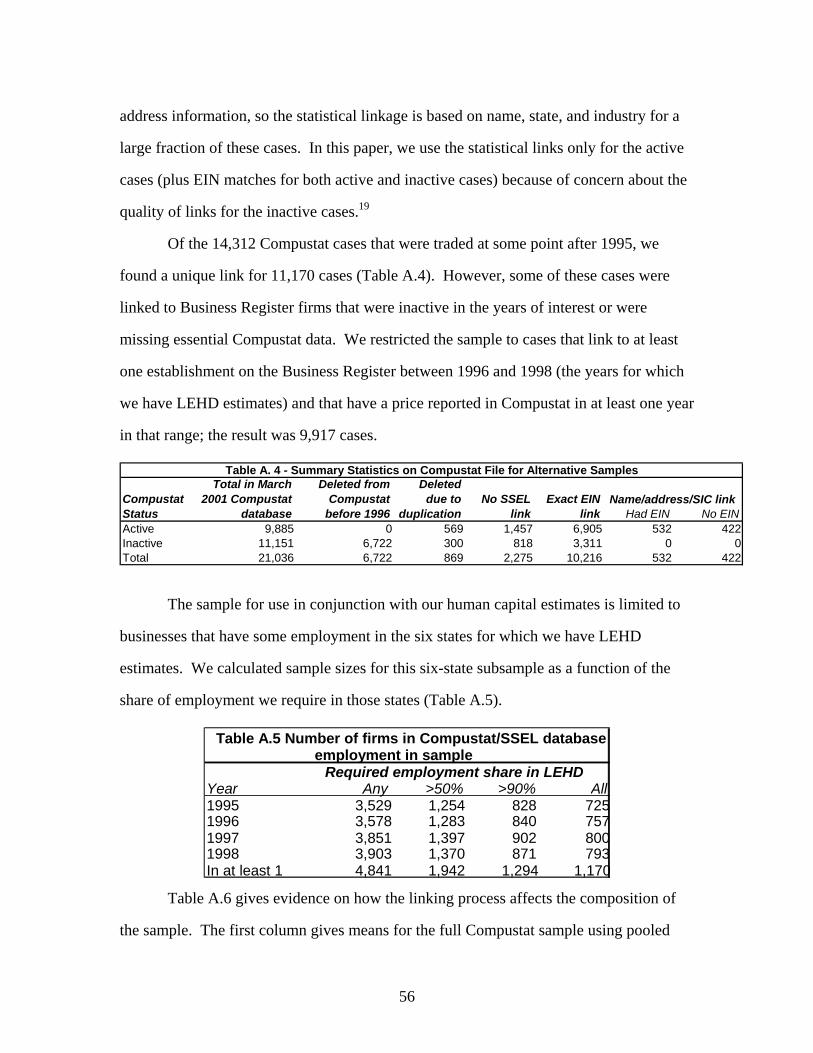
56

address information, so the statistical linkage is based on name, state, and industry for a

large fraction of these cases. In this paper, we use the statistical links only for the active

cases (plus EIN matches for both active and inactive cases) because of concern about the

quality of links for the inactive cases.19

Of the 14,312 Compustat cases that were traded at some point after 1995, we

found a unique link for 11,170 cases (Table A.4). However, some of these cases were

linked to Business Register firms that were inactive in the years of interest or were

missing essential Compustat data. We restricted the sample to cases that link to at least

one establishment on the Business Register between 1996 and 1998 (the years for which

we have LEHD estimates) and that have a price reported in Compustat in at least one year

in that range; the result was 9,917 cases.

Had EIN No EINActive 9,885 0 569 1,457 6,905 532 422Inactive 11,151 6,722 300 818 3,311 0 0Total 21,036 6,722 869 2,275 10,216 532 422

No SSEL link

Exact EIN link

Name/address/SIC link

Table A. 4 - Summary Statistics on Compustat File for Alternative Samples

Compustat Status

Total in March 2001 Compustat

database

Deleted from Compustat

before 1996

Deleted due to

duplication

The sample for use in conjunction with our human capital estimates is limited to

businesses that have some employment in the six states for which we have LEHD

estimates. We calculated sample sizes for this six-state subsample as a function of the

share of employment we require in those states (Table A.5).

Year Any >50% >90% All 1995 3,529 1,254 828 725 1996 3,578 1,283 840 757 1997 3,851 1,397 902 800 1998 3,903 1,370 871 793 In at least 1 4,841 1,942 1,294 1,170

Required employment share in LEHD

Table A.5 Number of firms in Compustat/SSEL database employment in sample

Table A.6 gives evidence on how the linking process affects the composition of

the sample. The first column gives means for the full Compustat sample using pooled

57

data from 1995-98 period for all Compustat cases that have nonmissing data on sales and

positive data on employment. The second column takes the subset of those cases that

were uniquely linked to a Business Register firm, and the third column further restricts

the sample to those with at least 50 percent of Business Register employment in the six

LEHD states.20

Full Compustat Matched Compustat/SSEL

Matched, with at least 50%

employment in LEHD states

Number of firms 32,613 22,911 4,367Market value $2,149 million $1,631 million $1,036 Compustat employment 6,281 5,068 2,925SSEL employment 3,497 1,878Sales, net $1,320 million $1,028 million $684 millionCompustat labor productivity (Sales/Employment) $363,000 $316,000 $358,000

Table A- 6 Sample means for full and matched samples

All three of these samples consist of firms that are very large simply because of

the restriction to publicly traded firms in Compustat. The matched samples have

somewhat smaller firms on average than the full Compustat sample. Very large, complex

firms may be more likely to be dropped in linking the two databases because of problems

with apparent duplication or because multinationals may not have an EIN in the database.

Very large companies are also more likely to have employment spread across many

states. Thus, they are less likely to be included in the third column of Table A.6.

Differences exist across the two data sources for employment, in part, probably,

because of the inclusion of overseas employees in the Compustat figures (the Business

Register data include only U.S. employees). However, detailed examination of the micro

data suggests that differences exist even for firms that operate only in the United States,

and the sources of those discrepancies are not clear. Possible candidates include

differences in the definition of employee or differences in the dating of employment (the

Business Register data reflect employment as of the week containing March 12, whereas

the Compustat employment numbers do not refer to a particular date).

58

For the Compustat variables, we follow the measurement methodology in the

literature (e.g., Hall, 1990, 1998; and BHY). We use the following primary Compustat

variables.

Market Value:

value of common stock at the end of the fiscal year plus preferred stock

value plus total debt. In Compustat mnemonics, it is

MKVALF+PSTK+DT.21

Physical Capital:

gross book value of capital stock is deflated by the GDP implicit price

deflator for fixed investment. The deflator is applied at the calculated

average age of the capital stock on the basis of the three-year average of

the ratio of total accumulated depreciation to current depreciation.

Other Assets:

total assets minus the book value of physical capital. This item includes

receivables, inventories, cash, and other accounting assets such as

goodwill reported by companies.

1

Endnotes 1 See ALM for details of the estimation procedure. Additional controls in x include year

effects interacted with gender effects and full-quarter employment adjustments (not all

workers work full quarters).

2 In most of the analysis that follows, we do not separate the effect of observable

characteristics, such as education, from those of unobservable components. For

subsamples of our universe files, we can measure education, and some of the results (see,

e.g,. in ALM) to which we refer are based upon such analysis. There is a large ongoing

effort at the LEHD Program to incorporate such observable characteristics on a more

comprehensive basis including the development of robust imputation procedures for our

universe files.

3 One issue that we do not explore here is the relation of the firm effects to productivity

and market value. Firm effects capture potentially many factors—rent sharing, firm

personnel policies, efficiency wages, and the effect of collective bargaining—that may be

positively or negatively related to productivity and market value. Identifying and

exploring these different effects is a rich area for future work. For more discussion of

this issue and related empirical work, see Abowd (1989, 1990).

4BHY specify a linear relation and emphasize the departure of coefficients from 1. Hall

(1998) discusses an alternative log linear relation that may be relevant. We use the log

linear specification in our analysis in part because our human capital measures are not on

the same inherent scale and metric as the measures of assets and market value.

5 In that sense, our approach is very much in the spirit of BHY.

2

6Cummins (in this volume) takes one approach to separate out some of these effects

(although not in the context of using measures of organizational or human capital). He

uses instrumental variable techniques to isolate the contribution of measures of tangible

assets by trying to find instruments that are correlated with the measured tangibles but

uncorrelated with unmeasured intangibles. As such, he attempts to identify the direct

effect of the measured assets. Moreover, his approach in principle avoids another related

problem of endogeneity arising from correlations of the asset variables with unmeasured

productivity or market value shocks. The unmeasured, idiosyncratic productivity and

market value shocks likely reflect, however, the idiosyncratic factors that we are seeking

to understand. The pursuit of an estimation strategy for instruments that are supposedly

orthogonal to these shocks may completely miss the role of intangibles.

7 In order to meet the requirements of the data use agreement between Census and the

individual states the identity of states used in a particular analysis is normally not

released

8 The identifiers in the LEHD Program’s human capital data provide additional

geographic and industry information but they are not coded down to the workplace

(establishment) level. Ongoing research is attempting to refine the most disaggregated

economic entity available in these data.

9 We use the two-digit SIC number as the industry measure in this work because,

although industries are coded at the four-digit level in the Economic Census and in the

underlying establishment data on the UI side, we have not yet implemented an algorithm

to use additional industrial or geographic detail in the definition of the establishment.

3

10 Recall that the level of aggregation that we use to approximate the establishment is that

of an EIN/SIC2/STATE cell. This unit is somewhere between the establishment and the

firm, but most firms operate only a single establishment.

11The official estimates include adjustments for changes in inventories in inventory-

holding sectors. However, studies by Foster, Haltiwanger, and Krizan (2001) show that,

in manufacturing, the correlation between labor productivity measured as shipments per

worker and labor productivity measured as shipments adjusted for inventory changes is

extremely high (almost 1).

12Note that the economy-wide thresholds are based on the universe of all workers in the

seven states (not just workers employed at the businesses we match to the Economic

Censuses) for which we have developed human capital estimates. We also generated

versions of these measures on the basis of thresholds relative to a specific industry rather

than the wider economy. The results were not sensitive to this distinction.

13 Because we use a log specification, we eliminate firms with missing or zero values.

This procedure creates an even smaller sample than the Compustat matched sample

described in the appendix. The excluded firms tend to have a greater fraction of skilled

workers, with greater representation in the upper tail of both the person effect and

experience components, and on average, the level of tenure of the workers in the

excluded firms is above average.

14 The reported results are based upon pooled data for 1995-98.

15 For this log linear specification, the coefficients on a particular asset (e.g., log of

physical capital) should reflect the share of that asset in the total.

4

16 A worker employed at the end of the first quarter is characterized as having worked for

that employer in both the first and second quarters.

17 Additional restrictions are imposed on the range of h, θ, and xβ values included in

these measures. If a worker has a value for h that is below 6 or above 14 or a value of θ

that is below –2 or above 2, that worker is excluded from the computation of the kernel-

density estimate at the business. This restriction removes only the extreme outliers and

results in a minor loss of both jobs and firms.

18 For example, some of the non-unique matches on the Business Register involve one

business that appears to be active and one that appears to be inactive. To match as many

cases as possible, we did not eliminate inactive establishments before matching but did so

afterward if the match was not unique. Some of the non-unique Compustat matches

involve cases that have a Compustat-assigned CUSIP, which often carries alternative

versions of data for companies that also have a standard CUSIP. For example, if an

acquisition took place in 1999, the data we have might contain two records for the

acquiring company: one with a standard CUSIP that has data reflecting the company’s

holdings in each year, and another with a Compustat-assigned CUSIP that has

consolidated data for the two businesses for some years before the merger. In this case,

we would drop the record with the Compustat-assigned CUSIP (and consolidated data)

and keep the record with the standard CUSIP.

19 Identifying the appropriate link was more complicated for the inactive cases both

because of a lack of detailed address information and because it was not clear at the

outset which years we should use for statistical linking. Because the statistical linking

was quite time intensive, we did not try to match all cases to all available years of the

5

Business Register, but rather tried first with earlier years and then worked forward if a

match was not found. After having identified links using that approach, we compared

years in which the identified firm was active on the Business Register to the years with

nonmissing data from Compustat. In a significant fraction of cases, the years did not line

up, and that problem was the main reason we decided not to use the 346 statistically

linked inactive cases.

20 The sample means in Table 6.1 are based on a sample with nonmissing data for a larger

set of variables and an additional link to the LEHD data. The final regression sample is

smaller than that in Table A.3 and has slightly smaller Compustat employment on

average (Table 6.1).

21Some differences in measurement methodology appear in the literature. Our method

most closely follows that of BHY. One difference is that Hall (1990) suggests adjusting

the value of long-term debt for differences in the age structure of the debt. However, in

the absence of firm-level information on the age structure of the debt, Hall assumes all

long-term debt has a 20-year maturity. One can readily develop scenarios in which this

assumption induces substantial measurement error.