The Reactor: A Sample-Efficient Actor-Critic … the actor is trained by a novel -leave-one-out policy gradient estimate (which uses both the off-policy corrected return and the estimated

Published as a conference paper at ICLR 2018

THE REACTOR:A FAST AND SAMPLE-EFFICIENT ACTOR-CRITICAGENT FOR REINFORCEMENT LEARNING

Audrunas Gruslys,[email protected]

Will Dabney,[email protected]

Mohammad Gheshlaghi Azar,[email protected]

Bilal Piot,[email protected]

Marc G. Bellemare,Google [email protected]

Rémi Munos,[email protected]

ABSTRACT

In this work, we present a new agent architecture, called Reactor, which combinesmultiple algorithmic and architectural contributions to produce an agent with highersample-efficiency than Prioritized Dueling DQN (Wang et al., 2017) and Categori-cal DQN (Bellemare et al., 2017), while giving better run-time performance thanA3C (Mnih et al., 2016). Our first contribution is a new policy evaluation algorithmcalled Distributional Retrace, which brings multi-step off-policy updates to thedistributional reinforcement learning setting. The same approach can be used toconvert several classes of multi-step policy evaluation algorithms, designed forexpected value evaluation, into distributional algorithms. Next, we introduce theβ-leave-one-out policy gradient algorithm, which improves the trade-off betweenvariance and bias by using action values as a baseline. Our final algorithmic con-tribution is a new prioritized replay algorithm for sequences, which exploits thetemporal locality of neighboring observations for more efficient replay prioritiza-tion. Using the Atari 2600 benchmarks, we show that each of these innovationscontribute to both sample efficiency and final agent performance. Finally, wedemonstrate that Reactor reaches state-of-the-art performance after 200 millionframes and less than a day of training.

1 INTRODUCTION

Model-free deep reinforcement learning has achieved several remarkable successes in domainsranging from super-human-level control in video games (Mnih et al., 2015) and the game of Go(Silver et al., 2016; 2017), to continuous motor control tasks (Lillicrap et al., 2015; Schulman et al.,2015).

Much of the recent work can be divided into two categories. First, those of which that, often buildingon the DQN framework, act ε-greedily according to an action-value function and train using mini-batches of transitions sampled from an experience replay buffer (Van Hasselt et al., 2016; Wang et al.,2015; He et al., 2017; Anschel et al., 2017). These value-function agents benefit from improvedsample complexity, but tend to suffer from long runtimes (e.g. DQN requires approximately a weekto train on Atari). The second category are the actor-critic agents, which includes the asynchronousadvantage actor-critic (A3C) algorithm, introduced by Mnih et al. (2016). These agents train ontransitions collected by multiple actors running, and often training, in parallel (Schulman et al., 2017;Vezhnevets et al., 2017). The deep actor-critic agents train on each trajectory only once, and thustend to have worse sample complexity. However, their distributed nature allows significantly fastertraining in terms of wall-clock time. Still, not all existing algorithms can be put in the above twocategories and various hybrid approaches do exist (Zhao et al., 2016; O’Donoghue et al., 2017; Guet al., 2017; Wang et al., 2017).

1

arX

iv:1

704.

0465

1v2

[cs

.AI]

19

Jun

2018


Data-efficiency and off-policy learning are essential for many real-world domains where interactionswith the environment are expensive. Similarly, wall-clock time (time-efficiency) directly impacts analgorithm’s applicability through resource costs. The focus of this work is to produce an agent thatis sample- and time-efficient. To this end, we introduce a new reinforcement learning agent, calledReactor (Retrace-Actor), which takes a principled approach to combining the sample-efficiency ofoff-policy experience replay with the time-efficiency of asynchronous algorithms. We combine recentadvances in both categories of agents with novel contributions to produce an agent that inherits thebenefits of both and reaches state-of-the-art performance over 57 Atari 2600 games.

Our primary contributions are (1) a novel policy gradient algorithm, β-LOO, which makes betteruse of action-value estimates to improve the policy gradient; (2) the first multi-step off-policydistributional reinforcement learning algorithm, distributional Retrace(λ); (3) a novel prioritizedreplay for off-policy sequences of transitions; and (4) an optimized network and parallel trainingarchitecture.

We begin by reviewing background material, including relevant improvements to both value-functionagents and actor-critic agents. In Section 3 we introduce each of our primary contributions andpresent the Reactor agent. Finally, in Section 4, we present experimental results on the 57 Atari 2600games from the Arcade Learning Environment (ALE) (Bellemare et al., 2013), as well as a series ofablation studies for the various components of Reactor.

2 BACKGROUND

We consider a Markov decision process (MDP) with state space X and finite action space A. A(stochastic) policy π(·|x) is a mapping from states x ∈ X to a probability distribution over actions.We consider a γ-discounted infinite-horizon criterion, with γ ∈ [0, 1) the discount factor, and definefor policy π the action-value of a state-action pair (x, a) as

Qπ(x, a)def= E

[∑t≥0γ

trt|x0 = x, a0 = a, π],

where ({xt}t≥0) is a trajectory generated by choosing a in x and following π thereafter, i.e., at ∼π(·|xt) (for t ≥ 1), and rt is the reward signal. The objective in reinforcement learning is tofind an optimal policy π∗, which maximises Qπ(x, a). The optimal action-values are given byQ∗(x, a) = maxπ Q

π(x, a).

2.1 VALUE-BASED ALGORITHMS

The Deep Q-Network (DQN) framework, introduced by Mnih et al. (2015), popularised the currentline of research into deep reinforcement learning by reaching human-level, and beyond, performanceacross 57 Atari 2600 games in the ALE. While DQN includes many specific components, the essenceof the framework, much of which is shared by Neural Fitted Q-Learning (Riedmiller, 2005), is touse of a deep convolutional neural network to approximate an action-value function, training thisapproximate action-value function using the Q-Learning algorithm (Watkins & Dayan, 1992) andmini-batches of one-step transitions (xt, at, rt, xt+1, γt) drawn randomly from an experience replaybuffer (Lin, 1992). Additionally, the next-state action-values are taken from a target network, whichis updated to match the current network periodically. Thus, the temporal difference (TD) error fortransition t used by these algorithms is given by

δt = rt + γt maxa′∈A

Q(xt+1, a′; θ)−Q(xt, at; θ), (1)

where θ denotes the parameters of the network and θ are the parameters of the target network.

Since this seminal work, we have seen numerous extensions and improvements that all sharethe same underlying framework. Double DQN (Van Hasselt et al., 2016), attempts to cor-rect for the over-estimation bias inherent in Q-Learning by changing the second term of (1) toQ(xt+1, arg maxa′∈AQ(xt+1, a

′; θ); θ). The dueling architecture (Wang et al., 2015), changes thenetwork to estimate action-values using separate network heads V (x; θ) and A(x, a; θ) with

Q(x, a; θ) = V (x; θ) +A(x, a; θ)− 1

|A|∑a′

A(x, a′; θ).

2


Recently, Hessel et al. (2017) introduced Rainbow, a value-based reinforcement learning agentcombining many of these improvements into a single agent and demonstrating that they are largelycomplementary. Rainbow significantly out performs previous methods, but also inherits the poorertime-efficiency of the DQN framework. We include a detailed comparison between Reactor andRainbow in the Appendix. In the remainder of the section we will describe in more depth other recentimprovements to DQN.

2.1.1 PRIORITIZED EXPERIENCE REPLAY

The experience replay buffer was first introduced by Lin (1992) and later used in DQN (Mnihet al., 2015). Typically, the replay buffer is essentially a first-in-first-out queue with new transitionsgradually replacing older transitions. The agent would then sample a mini-batch uniformly at randomfrom the replay buffer. Drawing inspiration from prioritized sweeping (Moore & Atkeson, 1993),prioritized experience replay replaces the uniform sampling with prioritized sampling proportional tothe absolute TD error (Schaul et al., 2016).

Specifically, for a replay buffer of size N , prioritized experience replay samples transition t withprobability P (t), and applies weighted importance-sampling with wt to correct for the prioritizationbias, where

P (t) =pαt∑k p

αk

, wt =

(1

N· 1

P (t)

)β, pt = |δt|+ ε, α, β, ε > 0. (2)

Prioritized DQN significantly increases both the sample-efficiency and final performance over DQNon the Atari 2600 benchmarks (Schaul et al., 2015).

2.1.2 RETRACE(λ)

Retrace(λ) is a convergent off-policy multi-step algorithm extending the DQN agent (Munos et al.,2016). Assume that some trajectory {x0, a0, r0, x1, a1, r1, . . . , xt, at, rt, . . . , } has been generatedaccording to behaviour policy µ, i.e., at ∼ µ(·|xt). Now, we aim to evaluate the value of a differenttarget policy π, i.e. we want to estimate Qπ . The Retrace algorithm will update our current estimateQ of Qπ in the direction of

∆Q(xt, at)def=∑s≥tγ

s−t(ct+1 . . . cs)δπsQ, (3)

where δπsQdef= rs + γEπ[Q(xs+1, ·)]−Q(xs, as) is the temporal difference at time s under π, and

cs = λmin(1, ρs

), ρs =

π(as|xs)µ(as|xs)

. (4)

The Retrace algorithm comes with the theoretical guarantee that in finite state and action spaces,repeatedly updating our current estimate Q according to (3) produces a sequence of Q functionswhich converges to Qπ for a fixed π or to Q∗ if we consider a sequence of policies π which becomeincreasingly greedy w.r.t. the Q estimates (Munos et al., 2016).

2.1.3 DISTRIBUTIONAL RL

Distributional reinforcement learning refers to a class of algorithms that directly estimate the distri-bution over returns, whose expectation gives the traditional value function (Bellemare et al., 2017).Such approaches can be made tractable with a distributional Bellman equation, and the recentlyproposed algorithm C51 showed state-of-the-art performance in the Atari 2600 benchmarks. C51parameterizes the distribution over returns with a mixture over Diracs centered on a uniform grid,

Q(x, a; θ) =

N−1∑i=0

qi(x, a; θ)zi, qi =eθi(x,a)∑N−1j=0 eθj(x,a)

, zi = vmin + ivmax − vmin

N − 1, (5)

with hyperparameters vmin, vmax that bound the distribution support of size N .

3


2.2 ACTOR-CRITIC ALGORITHMS

In this section we review the actor-critic framework for reinforcement learning algorithms andthen discuss recent advances in actor-critic algorithms along with their various trade-offs. Theasynchronous advantage actor-critic (A3C) algorithm (Mnih et al., 2016), maintains a parameterizedpolicy π(a|x; θ) and value function V (x; θv), which are updated with

4θ = ∇θ log π(at|xt; θ)A(xt, at; θv), 4θv = A(xt, at; θv)∇θvV (xt), (6)

where, A(xt, at; θv) =

n−1∑k

γkrt+k + γnV (xt+n)− V (xt). (7)

A3C uses M = 16 parallel CPU workers, each acting independently in the environment and applyingthe above updates asynchronously to a shared set of parameters. In contrast to the previously discussedvalue-based methods, A3C is an on-policy algorithm, and does not use a GPU nor a replay buffer.

Proximal Policy Optimization (PPO) is a closely related actor-critic algorithm (Schulman et al., 2017),which replaces the advantage (7) with,

min(ρtA(xt, at; θv), clip(ρt, 1− ε, 1 + ε)A(xt, at; θv)), ε > 0,

where ρt is as defined in Section 2.1.2. Although both PPO and A3C run M parallel workerscollecting trajectories independently in the environment, PPO collects these experiences to perform asingle, synchronous, update in contrast with the asynchronous updates of A3C.

Actor-Critic Experience Replay (ACER) extends the A3C framework with an experience replay buffer,Retrace algorithm for off-policy corrections, and the Truncated Importance Sampling LikelihoodRatio (TISLR) algorithm used for off-policy policy optimization (Wang et al., 2017).

3 THE REACTOR

The Reactor is a combination of four novel contributions on top of recent improvements to both deepvalue-based RL and policy-gradient algorithms. Each contribution moves Reactor towards our goalof achieving both sample and time efficiency.

3.1 β-LOO

The Reactor architecture represents both a policy π(a|x) and action-value function Q(x, a). We usea policy gradient algorithm to train the actor π which makes use of our current estimate Q(x, a) ofQπ(x, a). Let V π(x0) be the value function at some initial state x0, the policy gradient theorem saysthat ∇V π(x0) = E

[∑t γ

t∑aQ

π(xt, a)∇π(a|xt)], where ∇ refers to the gradient w.r.t. policy

parameters (Sutton et al., 2000). We now consider several possible ways to estimate this gradient.

To simplify notation, we drop the dependence on the state x for now and consider the problem ofestimating the quantity

G =∑aQ

π(a)∇π(a). (8)

In the off-policy case, we consider estimating G using a single action a drawn from a (possiblydifferent from π) behaviour distribution a ∼ µ. Let us assume that for the chosen action a we haveaccess to an unbiased estimate R(a) of Qπ(a). Then, we can use likelihood ratio (LR) methodcombined with an importance sampling (IS) ratio (which we call ISLR) to build an unbiased estimateof G:

GISLR =π(a)

µ(a)(R(a)− V )∇ log π(a),

where V is a baseline that depends on the state but not on the chosen action. However this estimatesuffers from high variance. A possible way for reducing variance is to estimate G directly from (8) byusing the return R(a) for the chosen action a and our current estimate Q of Qπ for the other actions,which leads to the so-called leave-one-out (LOO) policy-gradient estimate:

GLOO = R(a)∇π(a) +∑a 6=aQ(a)∇π(a). (9)

4


�E⇡

rt�E⇡

rt+1rt

�E⇡

1. Mix action-value distributions by ⇡

2. Shrink mixed distribution by �

3. Shift distribution by rt

4. Obtain target probabilities

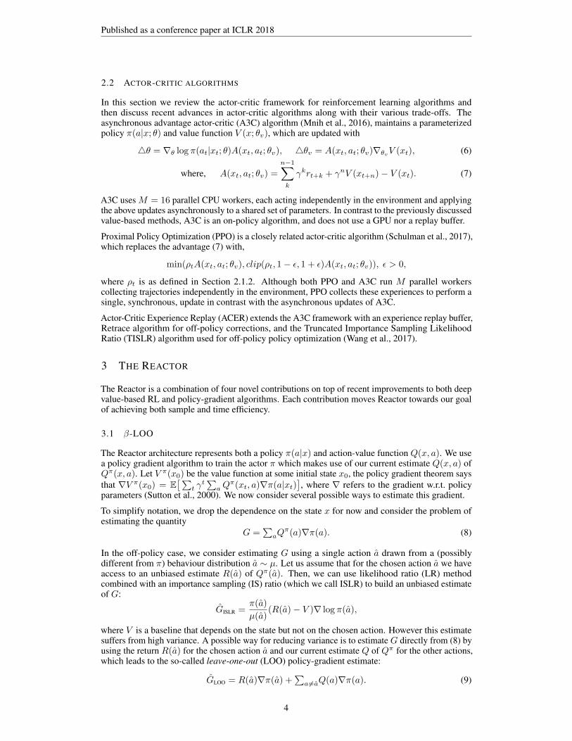
Figure 1: Single-step (left) and multi-step (right) distribution bootstrapping.

This estimate has low variance but may be biased if the estimated Q values differ from Qπ . A betterbias-variance tradeoff may be obtained by the more general β-LOO policy-gradient estimate:

Gβ-LOO = β(R(a)−Q(a))∇π(a) +∑aQ(a)∇π(a), (10)

where β = β(µ, π, a) can be a function of both policies, π and µ, and the selected action a. Noticethat when β = 1, (10) reduces to (9), and when β = 1/µ(a), then (10) is

G 1µ

-LOO =π(a)

µ(a)(R(a)−Q(a))∇ log π(a) +

∑aQ(a)∇π(a). (11)

This estimate is unbiased and can be seen as a generalization of GISLR where instead of using astate-only dependent baseline, we use a state-and-action-dependent baseline (our current estimate Q)and add the correction term

∑a∇π(a)Q(a) to cancel the bias. Proposition 1 gives our analysis of

the bias of Gβ-LOO, with a proof left to the Appendix.

Proposition 1. Assume a ∼ µ and that E[R(a)] = Qπ(a). Then, the bias of Gβ-LOO is∣∣∑

a(1 −µ(a)β(a))∇π(a)[Q(a)−Qπ(a)]

∣∣.Thus the bias is small when β(a) is close to 1/µ(a), or when the Q-estimates are close to the trueQπ values, and unbiased regardless of the estimates if β(a) = 1/µ(a). The variance is low when βis small, therefore, in order to improve the bias-variance tradeoff we recommend using the β-LOOestimate with β defined as: β(a) = min

(c, 1µ(a)

), for some constant c ≥ 1. This truncated 1/µ

coefficient shares similarities with the truncated IS gradient estimate introduced in (Wang et al., 2017)(which we call TISLR for truncated-ISLR):

GTISLR =min(c,π(a)

µ(a)

)(R(a)− V )∇ log π(a)+

∑a

(π(a)

µ(a)− c)+µ(a)(Qπ(a)− V )∇ log π(a).

The differences are: (i) we truncate 1/µ(a) = π(a)/µ(a)× 1/π(a) instead of truncating π(a)/µ(a),which provides an additional variance reduction due to the variance of the LR∇ log π(a) = ∇π(a)

π(a)

(since this LR may be large when a low probability action is chosen), and (ii) we use our Q-baselineinstead of a V baseline, reducing further the variance of the LR estimate.

3.2 DISTRIBUTIONAL RETRACE

In off-policy learning it is very difficult to produce an unbiased sampleR(a) ofQπ(a) when followinganother policy µ. This would require using full importance sampling correction along the trajectory.Instead, we use the off-policy corrected return computed by the Retrace algorithm, which produces a(biased) estimate of Qπ(a) but whose bias vanishes asymptotically (Munos et al., 2016).

In Reactor, we consider predicting an approximation of the return distribution function from anystate-action pair (x, a) in a similar way as in Bellemare et al. (2017). The original algorithm C51described in that paper considered single-step Bellman updates only. Here we need to extend thisidea to multi-step updates and handle the off-policy correction performed by the Retrace algorithm,as defined in (3). Next, we describe these two extensions.

Multi-step distributional Bellman operator: First, we extend C51 to multi-step Bellman backups.We consider return-distributions from (x, a) of the form

∑i qi(x, a)δzi (where δz denotes a Dirac in z)

5


which are supported on a finite uniform grid {zi} ∈ [vmin, vmax], zi < zi+1, z1 = vmin, zm = vmax.The coefficients qi(x, a) (discrete distribution) corresponds to the probabilities assigned to eachatom zi of the grid. From an observed n-step sequence {xt, at, rt, xt+1, . . . , xt+n}, generatedby behavior policy µ (i.e, as ∼ µ(·|xs) for t ≤ s < t + n), we build the n-step backed-upreturn-distribution from (xt, at). The n-step distributional Bellman target, whose expectation is∑t+n−1s=t γs−trs + γnQ(xt+n, a), is given by:

∑i

qi(xt+n, a)δzni , with zni =

t+n−1∑s=t

γs−trs + γnzi.

Since this distribution is supported on the set of atoms {zni }, which is not necessarily aligned withthe grid {zi}, we do a projection step and minimize the KL-loss between the projected target and thecurrent estimate, just as with C51 except with a different target distribution (Bellemare et al., 2017).

Distributional Retrace: Now, the Retrace algorithm defined in (3) involves an off-policy correctionwhich is not handled by the previous n-step distributional Bellman backup. The key to extending thisdistributional back-up to off-policy learning is to rewrite the Retrace algorithm as a linear combinationof n-step Bellman backups, weighted by some coefficients αn,a. Indeed, notice that (3) rewrites as

∆Q(xt, at) =∑n≥1

∑a∈A

αn,a

[ t+n−1∑s=t

γs−trs + γnQ(xt+n, a)︸︷︷︸n-step Bellman backup

]−Q(xt, at),

where αn,a =(ct+1 . . . ct+n−1

)(π(a|xt+n)− I{a = at+n}ct+n

). These coefficients depend on the

degree of off-policy-ness (between µ and π) along the trajectory. We have that∑n≥1

∑a αn,a =∑

n≥1(ct+1 . . . ct+n−1

)(1− ct+n) = 1, but notice some coefficients may be negative. However, in

expectation (over the behavior policy) they are non-negative. Indeed,

Eµ[αn,a] = E[(ct+1 . . . ct+n−1

)Eat+n∼µ(·|xt+n)

[π(a|xt+n)− I{a = at+n}ct+n|xt+n

]]= E

[(ct+1 . . . ct+n−1

)(π(a|xt+n)− µ(a|xt+n)λmin

(1,π(a|xt+n)

µ(a|xt+n)

))]≥ 0,

by definition of the cs coefficients (4). Thus in expectation (over the behavior policy), the Retraceupdate can be seen as a convex combination of n-step Bellman updates.

Then, the distributional Retrace algorithm can be defined as backing up a mixture of n-step distribu-tions. More precisely, we define the Retrace target distribution as:∑

i=1

q∗i (xt, at)δzi , with q∗i (xt, at) =∑n≥1

∑a

αn,a∑j

qj(xt+n, at+n)hzi(znj ),

where hzi(x) is a linear interpolation kernel, projecting onto the support {zi}:

hzi(x) =

(x− zi−1)/(zi − zi−1), if zi−1 ≤ x ≤ zi(zi+1 − x)/(zi+1 − zi), if zi ≤ x ≤ zi+1

0, if x ≤ zi−1 or x ≥ zi+1

1, if (x ≤ vmin and zi = vmin) or (x ≥ vmax and zi = vmax)

We update the current probabilities q(xt, at) by performing a gradient step on the KL-loss

∇KL(q∗(xt, at), q(xt, at)) = −∑i=1

q∗i (xt, at)∇ log qi(xt, at). (12)

Again, notice that some target “probabilities” q∗i (xt, at) may be negative for some sample trajectory,but in expectation they will be non-negative. Since the gradient of a KL-loss is linear w.r.t. its firstargument, our update rule (12) provides an unbiased estimate of the gradient of the KL between theexpected (over the behavior policy) Retrace target distribution and the current predicted distribution.1

1We store past action probabilities µ together with actions taken in the replay memory.

6


Remark: The same method can be applied to other algorithms (such as TB(λ) (Precup et al., 2000)and importance sampling (Precup et al., 2001)) in order to derive distributional versions of otheroff-policy multi-step RL algorithms.

3.3 PRIORITIZED SEQUENCE REPLAY

Prioritized experience replay has been shown to boost both statistical efficiency and final performanceof deep RL agents (Schaul et al., 2016). However, as originally defined prioritized replay does nothandle sequences of transitions and weights all unsampled transitions identically. In this section wepresent an alternative initialization strategy, called lazy initialization, and argue that it better encodesprior information about temporal difference errors. We then briefly describe our computationallyefficient prioritized sequence sampling algorithm, with full details left to the appendix.

It is widely recognized that TD errors tend to be temporally correlated, indeed the need to break thistemporal correlation has been one of the primary justifications for the use of experience replay (Mnihet al., 2015). Our proposed algorithm begins with this fundamental assumption.

Assumption 1. Temporal differences are temporally correlated, with correlation decaying on averagewith the time-difference between two transitions.

Prioritized experience replay adds new transitions to the replay buffer with a constant priority, butgiven the above assumption we can devise a better method. Specifically, we propose to add experienceto the buffer with no priority, inserting a priority only after the transition has been sampled and usedfor training. Also, instead of sampling transitions, we assign priorities to all (overlapping) sequencesof length n. When sampling, sequences with an assigned priority are sampled proportionally to thatpriority. Sequences with no assigned priority are sampled proportionally to the average priority ofassigned priority sequences within some local neighbourhood. Averages are weighted to compensatefor sampling biases (i.e. more samples are made in areas of high estimated priorities, and in theabsence of weighting this would lead to overestimation of unassigned priorities).

The lazy initialization scheme starts with priorities pt corresponding to the sequences{xt, at, . . . , xt+n} for which a priority was already assigned. Then it extrapolates a priority ofall other sequences in the following way. Let us define a partition (Ii)i of the states ordered byincreasing time such that each cell Ii contains exactly one state si with already assigned priority. Wedefine the estimated priority pt to all other sequences as pt =

∑si∈J(t)

wi∑i′∈J(t) wi′

p(si), where J(t)

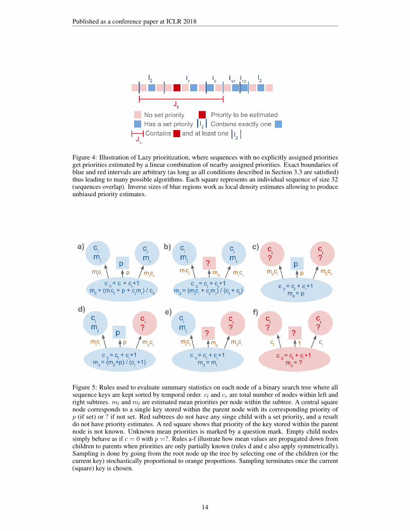
is a collection of contiguous cells (Ii) containing time t, and wi = |Ii| is the length of the cell Iicontaining si. For already defined priorities denote pt = pt. Cell sizes work as estimates of inverselocal density and are used as importance weights for priority estimation. 2 For the algorithm to beunbiased, partition (Ii)i must not be a function of the assigned priorities. So far we have defined aclass of algorithms all free to choose the partition (Ii) and the collection of cells I(t), as long thatthey satisfy the above constraints. Figure 4 in the Appendix illustrates the above description.

Now, with probability ε we sample uniformly at random, and with probability 1 − ε we sampleproportionally to pt. We implemented an algorithm satisfying the above constraints and called itContextual Priority Tree (CPT). It is based on AVL trees (Velskii & Landis, 1976) and can executesampling, insertion, deletion and density evaluation in O(ln(n)) time. We describe CPT in detail inthe Appendix in Section 6.3.

We treated prioritization as purely a variance reduction technique. Importance-sampling weightswere evaluated as in prioritized experience replay, with fixed β = 1 in (2). We used simple gradientmagnitude estimates as priorities, corresponding to a mean absolute TD error along a sequence forRetrace, as defined in (3) for the classical RL case, and total variation in the distributional Retracecase.3

3.4 AGENT ARCHITECTURE

In order to improve CPU utilization we decoupled acting from learning. This is an important aspectof our architecture: an acting thread receives observations, submits actions to the environment, and

2Not to be confused with importance weights of produced samples.3Sum of absolute discrete probability differences.

7


DQN

A3C

Reactor

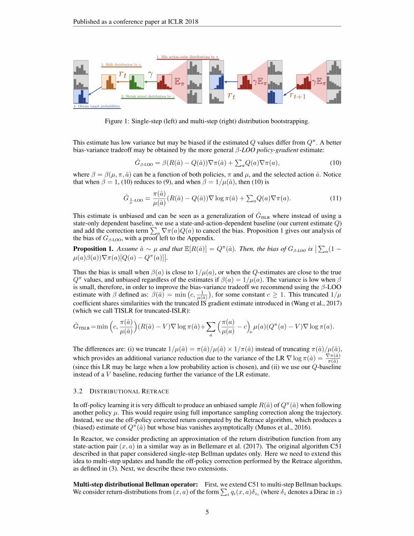
Algorithm Training Time Type # WorkersDQN 8 days GPU 1Double DQN 8 days GPU 1Dueling 8 days GPU 1Prioritized DQN 8 days GPU 1Rainbow 10 days GPU 1A3C 4 days CPU 16Reactor < 2 days CPU 10+1Reactor 500m 4 days CPU 10+1Reactor* < 1 day CPU 20+1

Figure 2: (Left) The model of parallelism of DQN, A3C and Reactor architectures. Each row represents aseparate thread. In Reactor’s case, each worker, consiting of a learner and an actor is run on a separate workermachine. (Right) Comparison of training times and resources for various algorithms. 500m denotes 500 milliontraining frames; otherwise 200m training frames were used.

stores transitions in memory, while a learning thread re-samples sequences of experiences frommemory and trains on them (Figure 2, left). We typically execute 4-6 acting steps per each learningstep. We sample sequences of length n = 33 in batches of 4. A moving network is unrolled overframes 1-32 while the target network is unrolled over frames 2-33.

We allow the agent to be distributed over multiple machines each containing action-learner pairs. Eachworker downloads the newest network parameters before each learning step and sends delta-updatesat the end of it. Both the network and target network are stored on a shared parameter server whileeach machine contains its own local replay memory. Training is done by downloading a sharednetwork, evaluating local gradients and sending them to be applied on the shared network. While theagent can also be trained on a single machine, in this work we present results of training obtainedwith either 10 or 20 actor-learner workers and one parameter server. In Figure 2 (right) we compareresources and runtimes of Reactor with related algorithms.4

3.4.1 NETWORK ARCHITECTURE

In some domains, such as Atari, it is useful to base decisions on a short history of past observations.The two techniques generally used to achieve this are frame stacking and recurrent network architec-tures. We chose the latter over the former for reasons of implementation simplicity and computationalefficiency. As the Retrace algorithm requires evaluating action-values over contiguous sequences oftrajectories, using a recurrent architecture allowed each frame to be processed by the convolutionalnetwork only once, as opposed to n times times if n frame concatenations were used.

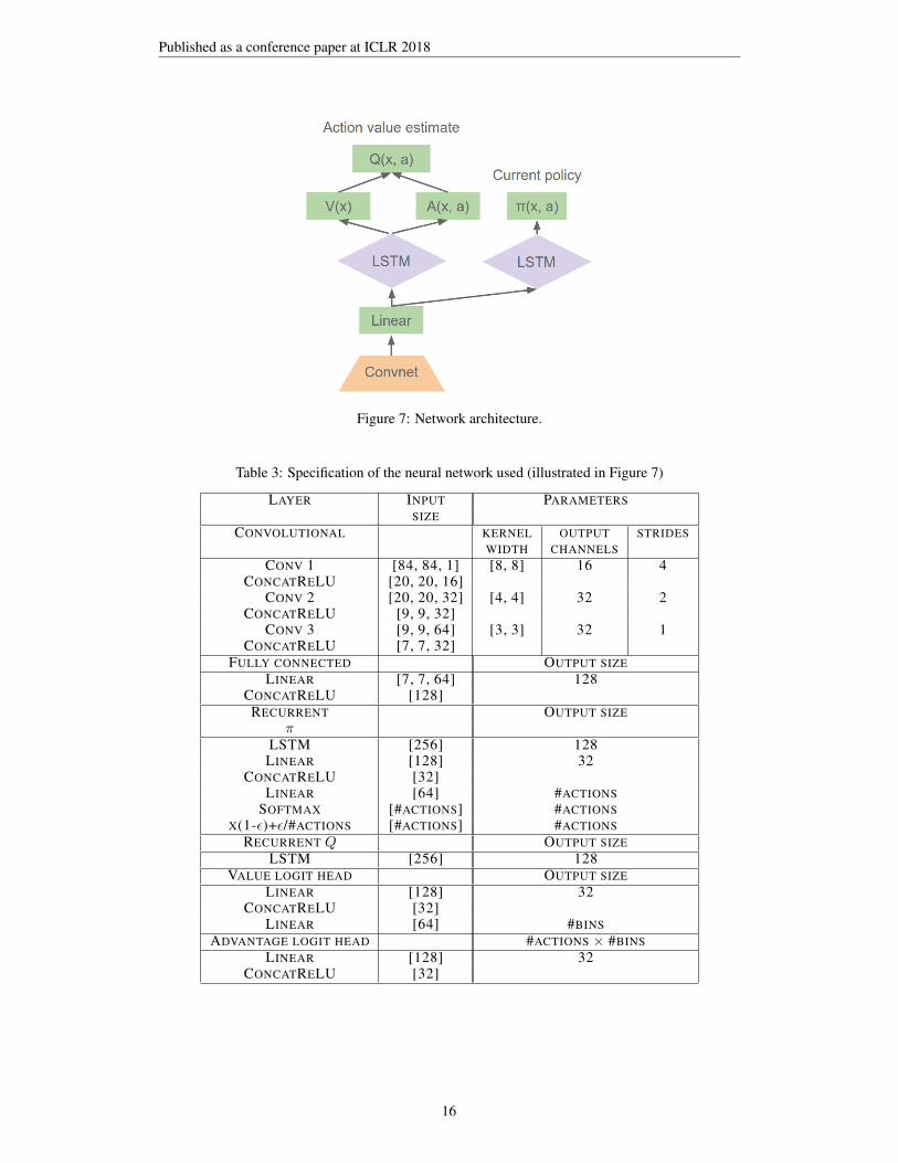
The Reactor architecture uses a recurrent neural network which takes an observation xt as input andproduces two outputs: categorical action-value distributions qi(xt, a) (i here is a bin identifier), andpolicy probabilities π(a|xt). We use an architecture inspired by the duelling network architecture(Wang et al., 2015). We split action-value -distribution logits into state-value logits and advantagelogits, which in turn are connected to the same LSTM network (Hochreiter & Schmidhuber, 1997).Final action-value logits are produced by summing state- and action-specific logits, as in Wang et al.(2015). Finally, a softmax layer on top for each action produces the distributions over discountedfuture returns.

The policy head uses a softmax layer mixed with a fixed uniform distribution over actions, wherethis mixing ratio is a hyperparameter (Wiering, 1999, Section 5.1.3). Policy and Q-networks haveseparate LSTMs. Both LSTMs are connected to a shared linear layer which is connected to a sharedconvolutional neural network (Krizhevsky et al., 2012). The precise network specification is given inTable 3 in the Appendix.

Gradients coming from the policy LSTM are blocked and only gradients originating from the Q-network LSTM are allowed to back-propagate into the convolutional neural network. We blockgradients from the policy head for increased stability, as this avoids positive feedback loops betweenπ and qi caused by shared representations. We used the Adam optimiser (Kingma & Ba, 2014),

4All results are reported with respect to the combined total number of observations obtained over all workermachines.

8


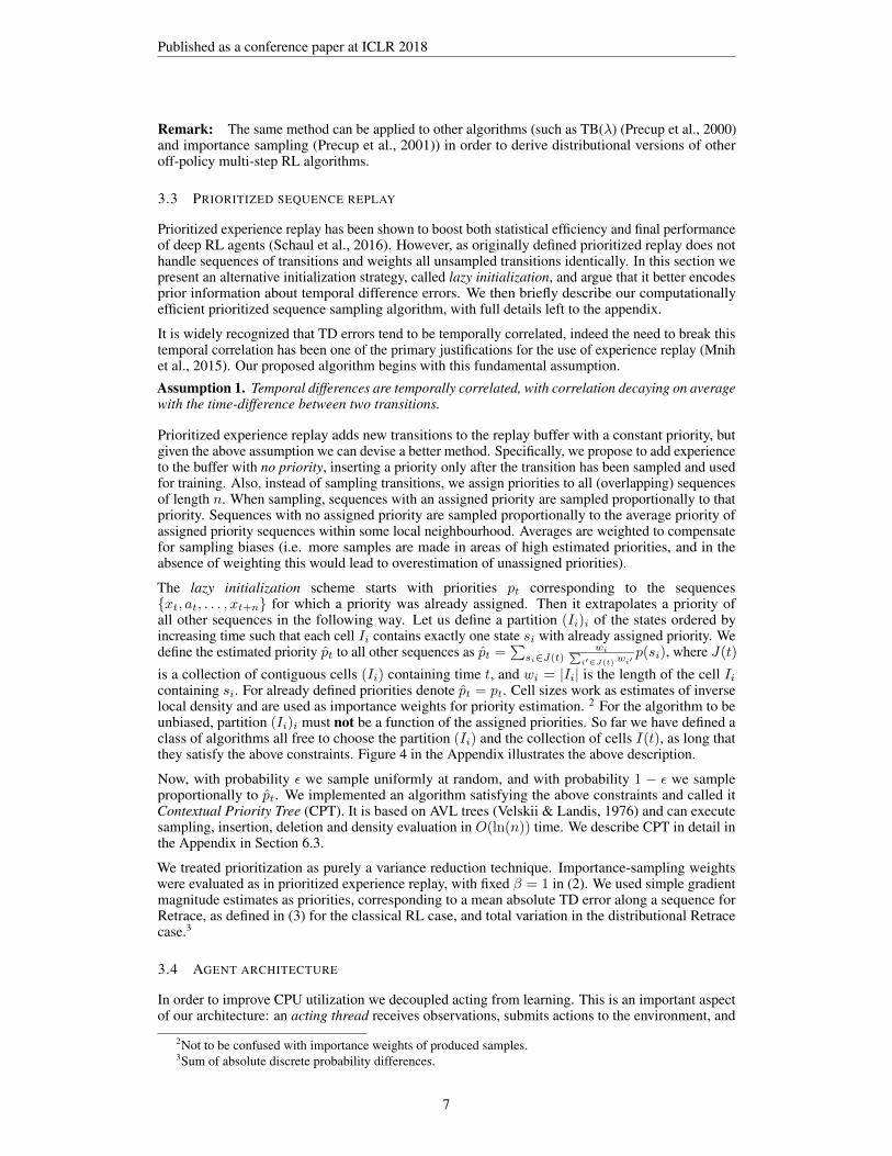
Figure 3: (Left) Reactor performance as various components are removed. (Right) Performance comparison asa function of training time in hours. Rainbow learning curve provided by Hessel et al. (2017).

with a learning rate of 5× 10−5 and zero momentum because asynchronous updates induce implicitmomentum (Mitliagkas et al., 2016). Further discussion of hyperparameters and their optimizationcan be found in Appendix 6.1.

4 EXPERIMENTAL RESULTS

We trained and evaluated Reactor on 57 Atari games (Bellemare et al., 2013). Figure 3 compares theperformance of Reactor with different versions of Reactor each time leaving one of the algorithmicimprovements out. We can see that each of the algorithmic improvements (Distributional retrace, beta-LOO and prioritized replay) contributed to the final results. While prioritization was arguably the mostimportant component, Beta-LOO clearly outperformed TISLR algorithm. Although distributionaland non-distributional versions performed similarly in terms of median human normalized scores,distributional version of the algorithm generalized better when tested with random human starts(Table 1).

ALGORITHM NORMALIZED MEAN ELOSCORES RANK

RANDOM 0.00 11.65 -563HUMAN 1.00 6.82 0

DQN 0.69 9.05 -172DDQN 1.11 7.63 -58DUEL 1.17 6.35 32PRIOR 1.13 6.63 13

PRIOR. DUEL. 1.15 6.25 40A3C LSTM 1.13 6.30 37RAINBOW 1.53 4.18 186

REACTOR ND 5 1.51 4.98 126REACTOR 1.65 4.58 156

REACTOR 500M 1.82 3.65 227

Table 1: Random human starts

ALGORITHM NORMALIZED MEAN ELOSCORES RANK

RANDOM 0.00 10.93 -673HUMAN 1.00 6.89 0

DQN 0.79 8.65 -167DDQN 1.18 7.28 -27DUEL 1.51 5.19 143PRIOR 1.24 6.11 70

PRIOR. DUEL. 1.72 5.44 126ACER6 500M 1.9 - -

RAINBOW 2.31 3.63 270REACTOR ND 5 1.80 4.53 195

REACTOR 1.87 4.46 196REACTOR 500M 2.30 3.47 280

Table 2: 30 random no-op starts.

4.1 COMPARING TO PRIOR WORK

We evaluated Reactor with target update frequency Tupdate = 1000, λ = 1.0 and β-LOO with β = 1on 57 Atari games trained on 10 machines in parallel. We averaged scores over 200 episodes using30 random human starts and noop starts (Tables 4 and 5 in the Appendix). We calculated mean andmedian human normalised scores across all games. We also ranked all algorithms (including randomand human scores) for each game and evaluated mean rank of each algorithm across all 57 Atarigames. We also evaluated mean Rank and Elo scores for each algorithm for both human and noopstart settings. Please refer to Section 6.2 in the Appendix for more details.

9


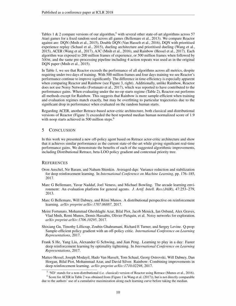
Tables 1 & 2 compare versions of our algorithm,5 with several other state-of-art algorithms across 57Atari games for a fixed random seed across all games (Bellemare et al., 2013). We compare Reactoragainst are: DQN (Mnih et al., 2015), Double DQN (Van Hasselt et al., 2016), DQN with prioritisedexperience replay (Schaul et al., 2015), dueling architecture and prioritised dueling (Wang et al.,2015), ACER (Wang et al., 2017), A3C (Mnih et al., 2016), and Rainbow (Hessel et al., 2017). Eachalgorithm was exposed to 200 million frames of experience, or 500 million frames when followed by500M, and the same pre-processing pipeline including 4 action repeats was used as in the originalDQN paper (Mnih et al., 2015).

In Table 1, we see that Reactor exceeds the performance of all algorithms across all metrics, despiterequiring under two days of training. With 500 million frames and four days training we see Reactor’sperformance continue to improve significantly. The difference in time-efficiency is especially apparentwhen comparing Reactor and Rainbow (see Figure 3, right). Additionally, unlike Rainbow, Reactordoes not use Noisy Networks (Fortunato et al., 2017), which was reported to have contributed to theperformance gains. When evaluating under the no-op starts regime (Table 2), Reactor out performsall methods except for Rainbow. This suggests that Rainbow is more sample-efficient when trainingand evaluation regimes match exactly, but may be overfitting to particular trajectories due to thesignificant drop in performance when evaluated on the random human starts.

Regarding ACER, another Retrace-based actor-critic architecture, both classical and distributionalversions of Reactor (Figure 3) exceeded the best reported median human normalized score of 1.9with noop starts achieved in 500 million steps.6

5 CONCLUSION

In this work we presented a new off-policy agent based on Retrace actor-critic architecture and showthat it achieves similar performance as the current state-of-the-art while giving significant real-timeperformance gains. We demonstrate the benefits of each of the suggested algorithmic improvements,including Distributional Retrace, beta-LOO policy gradient and contextual priority tree.

REFERENCES

Oron Anschel, Nir Baram, and Nahum Shimkin. Averaged-dqn: Variance reduction and stabilizationfor deep reinforcement learning. In International Conference on Machine Learning, pp. 176–185,2017.

Marc G Bellemare, Yavar Naddaf, Joel Veness, and Michael Bowling. The arcade learning envi-ronment: An evaluation platform for general agents. J. Artif. Intell. Res.(JAIR), 47:253–279,2013.

Marc G Bellemare, Will Dabney, and Rémi Munos. A distributional perspective on reinforcementlearning. arXiv preprint arXiv:1707.06887, 2017.

Meire Fortunato, Mohammad Gheshlaghi Azar, Bilal Piot, Jacob Menick, Ian Osband, Alex Graves,Vlad Mnih, Remi Munos, Demis Hassabis, Olivier Pietquin, et al. Noisy networks for exploration.arXiv preprint arXiv:1706.10295, 2017.

Shixiang Gu, Timothy Lillicrap, Zoubin Ghahramani, Richard E Turner, and Sergey Levine. Q-prop:Sample-efficient policy gradient with an off-policy critic. International Conference on LearningRepresentations, 2017.

Frank S He, Yang Liu, Alexander G Schwing, and Jian Peng. Learning to play in a day: Fasterdeep reinforcement learning by optimality tightening. In International Conference on LearningRepresentations, 2017.

Matteo Hessel, Joseph Modayil, Hado Van Hasselt, Tom Schaul, Georg Ostrovski, Will Dabney, DanHorgan, Bilal Piot, Mohammad Azar, and David Silver. Rainbow: Combining improvements indeep reinforcement learning. arXiv preprint arXiv:1710.02298, 2017.5 ‘ND‘ stands for a non-distributional (i.e. classical) version of Reactor using Retrace (Munos et al., 2016).6 Score for ACER in Table 2 was obtained from (Figure 1 in Wang et al. (2017)), but is not directly comparable

due to the authors’ use of a cumulative maximization along each learning curve before taking the median.

10


Sepp Hochreiter and Jürgen Schmidhuber. Long short-term memory. Neural computation, 9(8):1735–1780, 1997.

Diederik Kingma and Jimmy Ba. Adam: A method for stochastic optimization. arXiv preprintarXiv:1412.6980, 2014.

Alex Krizhevsky, Ilya Sutskever, and Geoffrey E Hinton. Imagenet classification with deep convolu-tional neural networks. In Advances in neural information processing systems, pp. 1097–1105,2012.

Timothy P Lillicrap, Jonathan J Hunt, Alexander Pritzel, Nicolas Heess, Tom Erez, Yuval Tassa,David Silver, and Daan Wierstra. Continuous control with deep reinforcement learning. arXivpreprint arXiv:1509.02971, 2015.

Long-H Lin. Self-improving reactive agents based on reinforcement learning, planning and teaching.Machine learning, 8(3/4):69–97, 1992.

Ioannis Mitliagkas, Ce Zhang, Stefan Hadjis, and Christopher Ré. Asynchrony begets momentum,with an application to deep learning. In Communication, Control, and Computing (Allerton), 201654th Annual Allerton Conference on, pp. 997–1004. IEEE, 2016.

Volodymyr Mnih, Koray Kavukcuoglu, David Silver, Andrei A Rusu, Joel Veness, Marc G Bellemare,Alex Graves, Martin Riedmiller, Andreas K Fidjeland, Georg Ostrovski, et al. Human-level controlthrough deep reinforcement learning. Nature, 518(7540):529–533, 2015.

Volodymyr Mnih, Adria Puigdomenech Badia, Mehdi Mirza, Alex Graves, Timothy P Lillicrap, TimHarley, David Silver, and Koray Kavukcuoglu. Asynchronous methods for deep reinforcementlearning. In International Conference on Machine Learning, 2016.

Andrew W Moore and Christopher G Atkeson. Prioritized sweeping: Reinforcement learning withless data and less time. Machine learning, 13(1):103–130, 1993.

Rémi Munos, Tom Stepleton, Anna Harutyunyan, and Marc Bellemare. Safe and efficient off-policyreinforcement learning. In Advances in Neural Information Processing Systems, pp. 1046–1054,2016.

Brendan O’Donoghue, Remi Munos, Koray Kavukcuoglu, and Volodymyr Mnih. Combining policygradient and q-learning. International Conference on Learning Representations, 2017.

Doina Precup, Richard S Sutton, and Satinder Singh. Eligibility traces for off-policy policy evaluation.In Proceedings of the Seventeenth International Conference on Machine Learning, 2000.

Doina Precup, Richard S Sutton, and Sanjoy Dasgupta. Off-policy temporal-difference learningwith function approximation. In Proceedings of the 18th International Conference on MachineLaerning, pp. 417–424, 2001.

Martin Riedmiller. Neural fitted q iteration-first experiences with a data efficient neural reinforcementlearning method. In ECML, volume 3720, pp. 317–328. Springer, 2005.

Tom Schaul, John Quan, Ioannis Antonoglou, and David Silver. Prioritized experience replay. arXivpreprint arXiv:1511.05952, 2015.

Tom Schaul, John Quan, Ioannis Antonoglou, and David Silver. Prioritized experience replay. InInternational Conference on Learning Representations, 2016.

John Schulman, Sergey Levine, Pieter Abbeel, Michael Jordan, and Philipp Moritz. Trust regionpolicy optimization. In Proceedings of the 32nd International Conference on Machine Learning(ICML-15), pp. 1889–1897, 2015.

John Schulman, Filip Wolski, Prafulla Dhariwal, Alec Radford, and Oleg Klimov. Proximal policyoptimization algorithms. arXiv preprint arXiv:1707.06347, 2017.

David Silver, Aja Huang, Chris J Maddison, Arthur Guez, Laurent Sifre, George Van Den Driessche,Julian Schrittwieser, Ioannis Antonoglou, Veda Panneershelvam, Marc Lanctot, et al. Masteringthe game of go with deep neural networks and tree search. Nature, 529(7587):484–489, 2016.

11


David Silver, Julian Schrittwieser, Karen Simonyan, Ioannis Antonoglou, Aja Huang, Arthur Guez,Thomas Hubert, Lucas Baker, Matthew Lai, Adrian Bolton, Yutian Chen, Timothy Lillicrap, FanHui, Laurent Sifre, George van den Driessche, Thore Graepel, and Demis Hassabis. Masteringthe game of go without human knowledge. Nature, 550(7676):354–359, 10 2017. URL http://dx.doi.org/10.1038/nature24270.

Richard S. Sutton, David Mcallester, Satinder Singh, and Yishay Mansour. Policy gradient methodsfor reinforcement learning with function approximation. In In Advances in Neural InformationProcessing Systems 12, pp. 1057–1063. MIT Press, 2000.

Hado Van Hasselt, Arthur Guez, and David Silver. Deep reinforcement learning with double q-learning. In AAAI, pp. 2094–2100, 2016.

Adel’son G Velskii and E Landis. An algorithm for the organisation of information. Dokl. Akad.Nauk SSSR, 146:263–266, 1976.

Alexander Sasha Vezhnevets, Simon Osindero, Tom Schaul, Nicolas Heess, Max Jaderberg, DavidSilver, and Koray Kavukcuoglu. Feudal networks for hierarchical reinforcement learning. arXivpreprint arXiv:1703.01161, 2017.

Ziyu Wang, Tom Schaul, Matteo Hessel, Hado van Hasselt, Marc Lanctot, and Nando de Freitas.Dueling network architectures for deep reinforcement learning. International Conference onMachine Learning, pp. 1995–2003, 2015.

Ziyu Wang, Victor Bapst, Nicolas Heess, Volodymyr Mnih, Remi Munos, Koray Kavukcuoglu, andNando de Freitas. Sample efficient actor-critic with experience replay. In International Conferenceon Learning Representations, 2017.

C. J. C. H. Watkins and P. Dayan. Q-learning. Machine Learning, 8(3):272–292, 1992.

Marco A Wiering. Explorations in efficient reinforcement learning. PhD thesis, University ofAmsterdam, 1999.

Dongbin Zhao, Haitao Wang, Kun Shao, and Yuanheng Zhu. Deep reinforcement learning withexperience replay based on sarsa. In Computational Intelligence (SSCI), 2016 IEEE SymposiumSeries on, pp. 1–6. IEEE, 2016.

12

http://dx.doi.org/10.1038/nature24270

http://dx.doi.org/10.1038/nature24270


6 APPENDIX

Proposition 1. Assume a ∼ µ and that E[R(a)] = Qπ(a). Then, the bias of Gβ-LOO is∣∣∑

a(1 −µ(a)β(a))∇π(a)[Q(a)−Qπ(a)]

∣∣.Proof. The bias of Gβ-LOO is

E[Gβ-LOO]−G =∑a

µ(a)[β(a)(E[R(a)]−Q(a))]∇π(a) +∑a

Q(a)∇π(a)−G

=∑a

(1− µ(a)β(a))[Q(a)−Qπ(a)]∇π(a)

6.1 HYPERPARAMETER OPTIMIZATION

As we believe that algorithms should be robust with respect to the choice of hyperparameters, wespent little effort on parameter optimization. In total, we explored three distinct values of learningrates and two values of ADAM momentum (the default and zero) and two values of Tupdate on asubset of 7 Atari games without prioritization using non-distributional version of Reactor. We laterused those values for all experiments. We did not optimize for batch sizes and sequence length or anyprioritization hyperparamters.

6.2 RANK AND ELO EVALUATION

Commonly used mean and median human normalized scores have several disadvantages. A meanhuman normalized score implicitly puts more weight on games that computers are good and humansare bad at. Comparing algorithm by a mean human normalized score across 57 Atari games isalmost equivalent to comparing algorithms on a small subset of games close to the median and thusdominating the signal. Typically a set of ten most score-generous games, namely Assault, Asterix,Breakout, Demon Attack, Double Dunk, Gopher, Pheonix, Stargunner, Up’n Down and Video Pinballcan explain more than half of inter-algorithm variance. A median human normalized score has theopposite disadvantage by effectively discarding very easy and very hard games from the comparison.As typical median human normalized scores are within the range of 1-2.5, an algorithm which scoreszero points on Montezuma’s Revenge is evaluated equal to the one which scores 2500 points, asboth performance levels are still below human performance making incremental improvements onhard games not being reflected in the overall evaluation. In order to address both problem, we alsoevaluated mean rank and Elo metrics for inter-algorithm comparison. Those metrics implicitly assignthe same weight to each game, and as a result is more sensitive of relative performance on very hardand easy games: swapping scores of two algorithms on any game would result in the change of bothmean rank and Elo metrics.

We calculated separate mean rank and Elo scores for each algorithm using results of test evaluationswith 30 random noop-starts and 30 random human starts (Tables 5 and 4). All algorithms were rankedacross each game separately, and a mean rank was evaluated across 57 Atari games. For Elo scoreevaluation algorithm, A was considered to win over algorithm B if it obtained more scores on a givenAtari. We produced an empirical win-probability matrix by summing wins across all games and usedthis matrix to evaluate Elo scores. A ranking difference of 400 corresponds to the odds of winning of10:1 under the Gaussian assumption.

6.3 CONTEXTUAL PRIORITY TREE

Contextual priority tree is one possible implementation of lazy prioritization (Figure 4). All sequencekeys are put into a balanced binary search tree which maintains a temporal order. An AVL tree(Velskii & Landis (1976)) was chosen due to the ease of implementation and because it is on averagemore evenly balanced than a Red-Black Tree.

Each tree node has up to two children (left and right) and contains currently stored key and a priorityof the key which is either set or is unknown. Some trees may only have a single child subtree while

13


Figure 4: Illustration of Lazy prioritization, where sequences with no explicitly assigned prioritiesget priorities estimated by a linear combination of nearby assigned priorities. Exact boundaries ofblue and red intervals are arbitrary (as long as all conditions described in Section 3.3 are satisfied)thus leading to many possible algorithms. Each square represents an individual sequence of size 32(sequences overlap). Inverse sizes of blue regions work as local density estimates allowing to produceunbiased priority estimates.

Figure 5: Rules used to evaluate summary statistics on each node of a binary search tree where allsequence keys are kept sorted by temporal order. cl and cr are total number of nodes within left andright subtrees. ml and ml are estimated mean priorities per node within the subtree. A central squarenode corresponds to a single key stored within the parent node with its corresponding priority ofp (if set) or ? if not set. Red subtrees do not have any singe child with a set priority, and a resultdo not have priority estimates. A red square shows that priority of the key stored within the parentnode is not known. Unknown mean priorities is marked by a question mark. Empty child nodessimply behave as if c = 0 with p =?. Rules a-f illustrate how mean values are propagated down fromchildren to parents when priorities are only partially known (rules d and e also apply symmetrically).Sampling is done by going from the root node up the tree by selecting one of the children (or thecurrent key) stochastically proportional to orange proportions. Sampling terminates once the current(square) key is chosen.

14


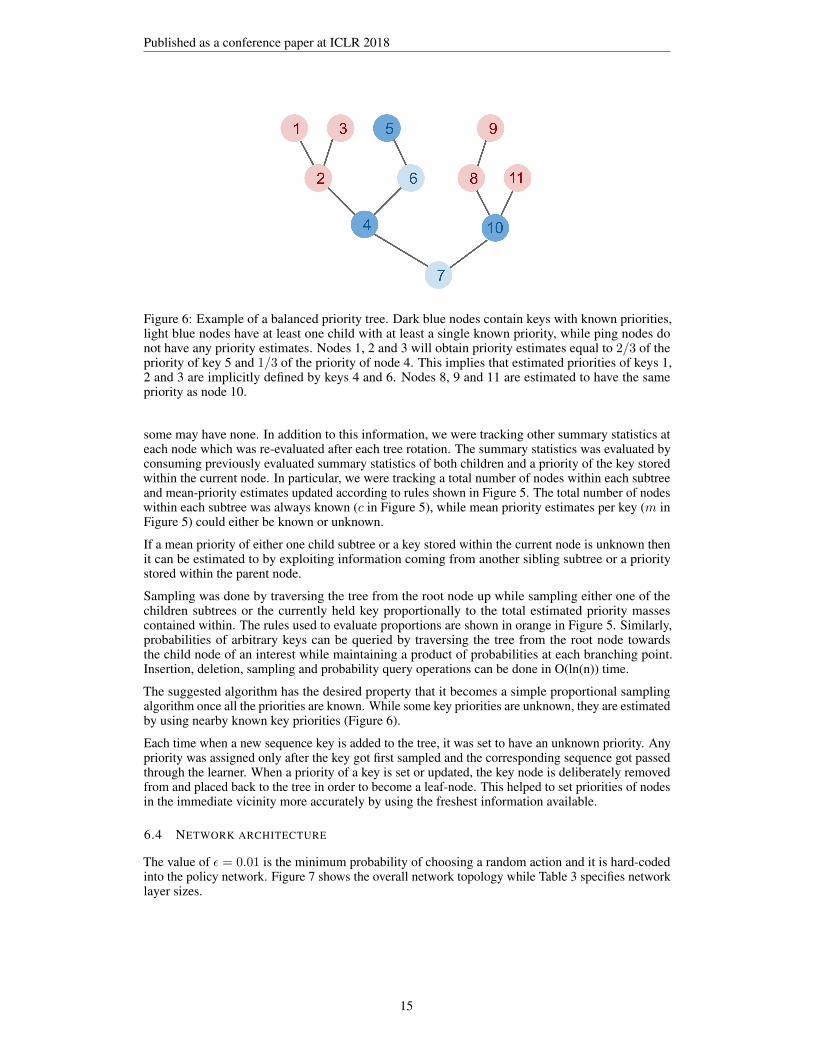
Figure 6: Example of a balanced priority tree. Dark blue nodes contain keys with known priorities,light blue nodes have at least one child with at least a single known priority, while ping nodes donot have any priority estimates. Nodes 1, 2 and 3 will obtain priority estimates equal to 2/3 of thepriority of key 5 and 1/3 of the priority of node 4. This implies that estimated priorities of keys 1,2 and 3 are implicitly defined by keys 4 and 6. Nodes 8, 9 and 11 are estimated to have the samepriority as node 10.

some may have none. In addition to this information, we were tracking other summary statistics ateach node which was re-evaluated after each tree rotation. The summary statistics was evaluated byconsuming previously evaluated summary statistics of both children and a priority of the key storedwithin the current node. In particular, we were tracking a total number of nodes within each subtreeand mean-priority estimates updated according to rules shown in Figure 5. The total number of nodeswithin each subtree was always known (c in Figure 5), while mean priority estimates per key (m inFigure 5) could either be known or unknown.

If a mean priority of either one child subtree or a key stored within the current node is unknown thenit can be estimated to by exploiting information coming from another sibling subtree or a prioritystored within the parent node.

Sampling was done by traversing the tree from the root node up while sampling either one of thechildren subtrees or the currently held key proportionally to the total estimated priority massescontained within. The rules used to evaluate proportions are shown in orange in Figure 5. Similarly,probabilities of arbitrary keys can be queried by traversing the tree from the root node towardsthe child node of an interest while maintaining a product of probabilities at each branching point.Insertion, deletion, sampling and probability query operations can be done in O(ln(n)) time.

The suggested algorithm has the desired property that it becomes a simple proportional samplingalgorithm once all the priorities are known. While some key priorities are unknown, they are estimatedby using nearby known key priorities (Figure 6).

Each time when a new sequence key is added to the tree, it was set to have an unknown priority. Anypriority was assigned only after the key got first sampled and the corresponding sequence got passedthrough the learner. When a priority of a key is set or updated, the key node is deliberately removedfrom and placed back to the tree in order to become a leaf-node. This helped to set priorities of nodesin the immediate vicinity more accurately by using the freshest information available.

6.4 NETWORK ARCHITECTURE

The value of ε = 0.01 is the minimum probability of choosing a random action and it is hard-codedinto the policy network. Figure 7 shows the overall network topology while Table 3 specifies networklayer sizes.

15


Figure 7: Network architecture.

Table 3: Specification of the neural network used (illustrated in Figure 7)

LAYER INPUT PARAMETERSSIZE

CONVOLUTIONAL KERNEL OUTPUT STRIDESWIDTH CHANNELS

CONV 1 [84, 84, 1] [8, 8] 16 4CONCATRELU [20, 20, 16]

CONV 2 [20, 20, 32] [4, 4] 32 2CONCATRELU [9, 9, 32]

CONV 3 [9, 9, 64] [3, 3] 32 1CONCATRELU [7, 7, 32]

FULLY CONNECTED OUTPUT SIZELINEAR [7, 7, 64] 128

CONCATRELU [128]RECURRENT OUTPUT SIZE

πLSTM [256] 128LINEAR [128] 32

CONCATRELU [32]LINEAR [64] #ACTIONS

SOFTMAX [#ACTIONS] #ACTIONSX(1-ε)+ε/#ACTIONS [#ACTIONS] #ACTIONS

RECURRENT Q OUTPUT SIZELSTM [256] 128

VALUE LOGIT HEAD OUTPUT SIZELINEAR [128] 32

CONCATRELU [32]LINEAR [64] #BINS

ADVANTAGE LOGIT HEAD #ACTIONS × #BINSLINEAR [128] 32

CONCATRELU [32]

16


6.5 COMPARISONS WITH RAINBOW

In this section we compare Reactor with the recently published Rainbow agent (Hessel et al., 2017).While ACER is the most closely related algorithmically, Rainbow is most closely related in terms ofperformance and thus a deeper understanding of the trade-offs between Rainbow and Reactor maybenefit interested readers. There are many architectural and algorithmic differences between Rainbowand Reactor. We will therefore begin by highlighting where they agree. Both use a categoricalaction-value distribution critic (Bellemare et al., 2017), factored into state and state-action logits(Wang et al., 2015),

qi(x, a) =li(x, a)∑j lj(x, a)

, li(x, a) = li(x) + li(x, a)− 1

|A|∑b∈A

li(x, b).

Both use prioritized replay, and finally, both perform n-step Bellman updates.

Despite these similarities, Reactor and Rainbow are fundamentally different algorithms and are basedupon different lines of research. While Rainbow uses Q-Learning and is based upon DQN (Mnihet al., 2015), Reactor is an actor-critic algorithm most closely based upon A3C (Mnih et al., 2016).Each inherits some design choices from their predecessors, and we have not performed an extensiveablation comparing these various differences. Instead, we will discuss four of the differences webelieve are important but less obvious.

First, the network structures are substantially different. Rainbow uses noisy linear layers and ReLUactivations throughout the network, whereas Reactor uses standard linear layers and concatenatedReLU activations throughout. To overcome partial observability, Rainbow, inheriting this choicefrom DQN, uses frame stacking. On the other hand, Reactor, inheriting its choice from A3C, usesLSTMs after the convolutional layers of the network. It is also difficult to directly compare thenumber of parameters in each network because the use of noisy linear layers doubles the number ofparameters, although half of these are used to control noise, while the LSTM units in Reactor requiremore parameters than a corresponding linear layer would.

Second, both algorithms perform n-step updates, however, the Rainbow n-step update does not useany form of off-policy correction. Because of this, Rainbow is restricted to using only small values ofn (e.g. n = 3) because larger values would make sequences more off-policy and hurt performance.By comparison, Reactor uses our proposed distributional Retrace algorithm for off-policy correctionof n-step updates. This allows the use of larger values of n (e.g. n = 33) without loss of performance.

Third, while both agents use prioritized replay buffers (Schaul et al., 2016), they each store differentinformation and prioritize using different algorithms. Rainbow stores a tuple containing the state xt−1,action at−1, sum of n discounted rewards

∑n−1k=0 rt+k

∏k−1m=0 γt+m, product of n discount factors∏n−1

k=0 γt+k, and next-state n steps away xt+n−1. Tuples are prioritized based upon the last observedTD error, and inserted into replay with a maximum priority. Reactor stores length n sequences oftuples (xt−1, at−1, rt, γt) and also prioritizes based upon the observed TD error. However, wheninserted into the buffer the priority is instead inferred based upon the known priorities of neighboringsequences. This priority inference was made efficient using the previously introduced contextualpriority tree, and anecdotally we have seen it improve performance over a simple maximum priorityapproach.

Finally, the two algorithms have different approaches to exploration. Rainbow, unlike DQN, doesnot use ε-greedy exploration, but instead replaces all linear layers with noisy linear layers whichinduce randomness throughout the network. This method, called Noisy Networks (Fortunato et al.,2017), creates an adaptive exploration integrated into the agent’s network. Reactor does not usenoisy networks, but instead uses the same entropy cost method used by A3C and many others (Mnihet al., 2016), which penalizes deterministic policies thus encouraging indifference between similarlyvalued actions. Because Rainbow can essentially learn not to explore, it may learn to become entirelygreedy in the early parts of the episode, while still exploring in states not as frequently seen. Insome sense, this is precisely what we want from an exploration technique, but it may also lead tohighly deterministic trajectories in the early part of the episode and an increase in overfitting tothose trajectories. We hypothesize that this may be the explanation for the significant difference inRainbow’s performance between evaluation under no-op and random human starts, and why Reactordoes not show such a large difference.

17


6.6 ATARI RESULTS

Table 4: Scores for each game evaluated with 30 random human starts. Reactor was evaluated byaveraging scores over 200 episodes. All scores (except for Reactor) were taken from Wang et al.(2015), Mnih et al. (2016) and Hessel et al. (2017).

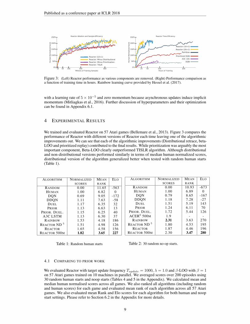
Table 5: Scores for each game evaluated with 30 random noop starts. Reactor was evaluated byaveraging scores over 200 episodes. All scores (except for Reactor) were taken from Wang et al.(2015) and Hessel et al. (2017).

GAME AGENT RANDOM HUMAN DQN DDQN DUEL PRIOR PRIOR.DUEL.

RAINBOW REACTORND 5

REACTOR REACTOR500M

ALIEN 227.8 7127.7 1620.0 3747.7 4461.4 4203.8 3941.0 9491.7 4199.4 6482.1 12689.1AMIDAR 5.8 1719.5 978.0 1793.3 2354.5 1838.9 2296.8 5131.2 1546.8 833.0 1015.8ASSAULT 222.4 742.0 4280.4 5393.2 4621.0 7672.1 11477.0 14198.5 17543.8 11013.5 8323.3ASTERIX 210.0 8503.3 4359.0 17356.5 28188.0 31527.0 375080.0 428200.3 16121.0 36238.5 205914.0ASTEROIDS 719.1 47388.7 1364.5 734.7 2837.7 2654.3 1192.7 2712.8 4467.4 2780.4 3726.1ATLANTIS 12850.0 29028.1 279987.0 106056.0 382572.0 357324.0 395762.0 826659.5 968179.5 308258.0 302831.0BANK HEIST 14.2 753.1 455.0 1030.6 1611.9 1054.6 1503.1 1358.0 1236.8 988.7 1259.7BATTLEZONE 2360.0 37187.5 29900.0 31700.0 37150.0 31530.0 35520.0 62010.0 98235.0 61220.0 64070.0BEAM RIDER 363.9 16926.5 8627.5 13772.8 12164.0 23384.2 30276.5 16850.2 8811.8 8566.5 11033.4BERZERK 123.7 2630.4 585.6 1225.4 1472.6 1305.6 3409.0 2545.6 1515.7 1641.4 2303.1BOWLING 23.1 160.7 50.4 68.1 65.5 47.9 46.7 30.0 59.3 75.4 81.0BOXING 0.1 12.1 88.0 91.6 99.4 95.6 98.9 99.6 99.7 99.4 99.4BREAKOUT 1.7 30.5 385.5 418.5 345.3 373.9 366.0 417.5 509.5 518.4 514.8CENTIPEDE 2090.9 12017.0 4657.7 5409.4 7561.4 4463.2 7687.5 8167.3 7267.2 3402.8 3422.0CHOPPER COMMAND 811.0 7387.8 6126.0 5809.0 11215.0 8600.0 13185.0 16654.0 19901.5 37568.0 107779.0CRAZY CLIMBER 10780.5 35829.4 110763.0 117282.0 143570.0 141161.0 162224.0 168788.5 173274.0 194347.0 236422.0DEFENDER 2874.5 18688.9 23633.0 35338.5 42214.0 31286.5 41324.5 55105.0 181074.3 113128.0 223025.0DEMON ATTACK 152.1 1971.0 12149.4 58044.2 60813.3 71846.4 72878.6 111185.2 122782.5 100189.0 115154.0DOUBLE DUNK -18.6 -16.4 -6.6 -5.5 0.1 18.5 -12.5 -0.3 23.0 11.4 23.0ENDURO 0.0 860.5 729.0 1211.8 2258.2 2093.0 2306.4 2125.9 2211.3 2230.1 2224.2FISHING DERBY -91.7 -38.7 -4.9 15.5 46.4 39.5 41.3 31.3 33.1 23.2 30.4FREEWAY 0.0 29.6 30.8 33.3 0.0 33.7 33.0 34.0 22.3 31.4 31.5FROSTBITE 65.2 4334.7 797.4 1683.3 4672.8 4380.1 7413.0 9590.5 7136.7 8042.1 7932.2GOPHER 257.6 2412.5 8777.4 14840.8 15718.4 32487.2 104368.2 70354.6 36279.1 69135.1 89851.0GRAVITAR 173.0 3351.4 473.0 412.0 588.0 548.5 238.0 1419.3 1804.8 1073.8 2041.8H.E.R.O. 1027.0 30826.4 20437.8 20130.2 20818.2 23037.7 21036.5 55887.4 27833.0 35542.2 43360.4ICE HOCKEY -11.2 0.9 -1.9 -2.7 0.5 1.3 -0.4 1.1 15.7 3.4 10.7JAMES BOND 007 29.0 302.8 768.5 1358.0 1312.5 5148.0 812.0 19809.0 14524.0 7869.2 16056.2KANGAROO 52.0 3035.0 7259.0 12992.0 14854.0 16200.0 1792.0 14637.5 13349.0 10484.5 11266.5KRULL 1598.0 2665.5 8422.3 7920.5 11451.9 9728.0 10374.4 8741.5 10237.8 9930.8 9896.0KUNG-FU MASTER 258.5 22736.3 26059.0 29710.0 34294.0 39581.0 48375.0 52181.0 61621.5 59799.5 65836.5MONTEZUMA’S REVENGE 0.0 4753.3 0.0 0.0 0.0 0.0 0.0 384.0 0.0 2643.5 2643.5MS. PAC-MAN 307.3 6951.6 3085.6 2711.4 6283.5 6518.7 3327.3 5380.4 4416.9 2724.3 3749.2NAME THIS GAME 2292.3 8049.0 8207.8 10616.0 11971.1 12270.5 15572.5 13136.0 12636.5 9907.2 9543.8PHOENIX 761.4 7242.6 8485.2 12252.5 23092.2 18992.7 70324.3 108528.6 10261.4 40092.2 46536.4PITFALL! -229.4 6463.7 -286.1 -29.9 0.0 -356.5 0.0 0.0 -3.7 -3.5 -8.9PONG -20.7 14.6 19.5 20.9 21.0 20.6 20.9 20.9 20.7 20.7 20.6PRIVATE EYE 24.9 69571.3 146.7 129.7 103.0 200.0 206.0 4234.0 15198.0 15177.1 15188.8Q*BERT 163.9 13455.0 13117.3 15088.5 19220.3 16256.5 18760.3 33817.5 21222.5 22956.5 21509.2RIVER RAID 1338.5 17118.0 7377.6 14884.5 21162.6 14522.3 20607.6 22920.8 16957.3 16608.3 17380.7ROAD RUNNER 11.5 7845.0 39544.0 44127.0 69524.0 57608.0 62151.0 62041.0 66790.5 71168.0 111310.0ROBOTANK 2.2 11.9 63.9 65.1 65.3 62.6 27.5 61.4 71.8 68.5 70.4SEAQUEST 68.4 42054.7 5860.6 16452.7 50254.2 26357.8 931.6 15898.9 5071.6 8425.8 20994.1SKIING -17098.1 -4336.9 -13062.3 -9021.8 -8857.4 -9996.9 -19949.9 -12957.8 -10632.9 -10753.4 -10870.6SOLARIS 1236.3 12326.7 3482.8 3067.8 2250.8 4309.0 133.4 3560.3 2236.0 2760.0 2099.6SPACE INVADERS 148.0 1668.7 1692.3 2525.5 6427.3 2865.8 15311.5 18789.0 2387.1 2448.6 10153.9STARGUNNER 664.0 10250.0 54282.0 60142.0 89238.0 63302.0 125117.0 127029.0 48942.0 70038.0 79521.5SURROUND -10.0 6.5 -5.6 -2.9 4.4 8.9 1.2 9.7 0.9 6.7 7.0TENNIS -23.8 -8.3 12.2 -22.8 5.1 0.0 0.0 0.0 23.4 23.3 23.6TIME PILOT 3568.0 5229.2 4870.0 8339.0 11666.0 9197.0 7553.0 12926.0 18871.5 19401.0 18841.5TUTANKHAM 11.4 167.6 68.1 218.4 211.4 204.6 245.9 241.0 263.2 272.6 275.4UP’N DOWN 533.4 11693.2 9989.9 22972.2 44939.6 16154.1 33879.1 125754.6 194989.5 64354.2 70790.4VENTURE 0.0 1187.5 163.0 98.0 497.0 54.0 48.0 5.5 0.0 1597.5 1653.5VIDEO PINBALL 16256.9 17667.9 196760.4 309941.9 98209.5 282007.3 479197.0 533936.5 261720.2 469366.0 496101.0WIZARD OF WOR 563.5 4756.5 2704.0 7492.0 7855.0 4802.0 12352.0 17862.5 18484.0 13170.5 19530.5YARS’ REVENGE 3092.9 54576.9 18098.9 11712.6 49622.1 11357.0 69618.1 102557.0 109607.5 102760.0 148855.0ZAXXON 32.5 9173.3 5363.0 10163.0 12944.0 10469.0 13886.0 22209.5 16525.0 25215.5 27582.5

18

Documents

The Reactor: A Sample-Efficient Actor-Critic … the actor is trained by a novel -leave-one-out policy gradient estimate (which uses both the off-policy corrected return and the estimated