Embed Size (px)
Citation preview

U.S. DEPARTMENT OF COMMERCE
National Oceanic and Atmospheric Administration
National Marine Fisheries Service
The Raymond J. H. Beverton Lectures at Woods Hole, Massachusetts


The Raymond J. H. Beverton Lectures
at Woods Hole, Massachusetts


The Raymond J. H. Beverton Lectures
at Woods Hole, Massachusetts
Three Lectures on Fisheries ScienceGiven May 2–3, 1994
Edited by Emory D. Anderson
May 2002NOAA Technical Memorandum NMFS-F/SPO-54
U.S. DEPARTMENT OF COMMERCE Donald L. Evans, Secretary
National Oceanic and Atmospheric Administration Vice Admiral Conrad C. Lautenbacher, Jr., U.S. Navy (Ret.),
Under Secretary for Oceans and Atmosphere
National Marine Fisheries Service William T. Hogarth, Assistant Administrator for Fisheries

AN
OT
AN
LO
CEA
NICAND ATMOSPHERIC
ADMIN
IS
U.S
. DEPARTMENT OF COMM
ERC
E
TRA
IT
N
O
This entire publication may be cited as:
Anderson, E. D. (Editor). 2002. The Raymond J. H. Beverton lectures at Woods Hole, Massachusetts. Three Lectures on Fisheries Science Given May 2–3, 1994. U.S. Dep. Commer., NOAA Tech. Memo. NMFS-F/SPO-54, 161 p.
Invididual lectures from the publication may be cited as in this example of Lecture 1:
Beverton, R. J. H. 2002. Man or Nature in Fisheries Dynamics: Who Calls the Tune? In E. D. Anderson (Editor), The Raymond J. H. Beverton lectures at Woods Hole, Massachusetts. Three Lectures on Fisheries Science Given May 2–3, 1994, p. 9–59. U.S. Dep. Commer., NOAA Tech. Memo. NMFS-F/SPO-54.
For sale by the Superintendent of Documents, U.S. Government Printing Office, Washington, DC 20402.Telephone orders: 866-512-1800 (toll-free), 202-512-1800 (for calls from the DC area)Facsimile orders: 202-512-2250Internet orders (secure on-line ordering): http://bookstore.gpo.govMail orders: Superintendent of Documents
PO Box 371954 Pittsburgh, PA 15250-7954
An online version of this publication is available at http://spo.nwr.noaa.gov/BevertonLectures1994/
This publication is printed on recycled paper with vegetable-based ink.
ISBN 0-9722532-1-1
(✩ ) U.S. Government Printing Office, 2002—791-811.
I
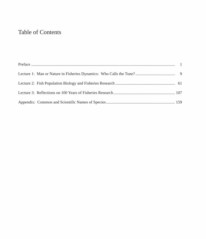
Table of Contents
Preface .............................................................................................................................................. 1
Lecture 1: Man or Nature in Fisheries Dynamics: Who Calls the Tune? ....................................... 9
Lecture 2: Fish Population Biology and Fisheries Research ........................................................... 61
Lecture 3: Reflections on 100 Years of Fisheries Research............................................................. 107
Appendix: Common and Scientific Names of Species .................................................................... 159


Preface


In May 1994, Ray Beverton presented a series of lectures at facilities of NOAA’s National
Marine Fisheries Service (NMFS) in Woods Hole, Mass.; Seattle, Wash.; Auke Bay and Juneau, Alaska; La Jolla, Calif.; Beaufort, N.C.; and Silver Spring, Md. This tour was initiated and organized by Michael Sissenwine, NMFS Senior Scientist at the time, and sponsored by NMFS.
The NMFS Northeast Fisheries Science Center (NEFSC) in Woods Hole was the first stop on Ray’s itinerary, and it was my honor and privilege to welcome and introduce him at the first of his three lectures during May 2–3. My wife, Geri, and I also had the pleasure of hosting Ray and his wife, Kathy, at our home during those few days.
Ray was kept quite busy during his 2-day stint in Woods Hole. He delivered the first lecture entitled “Man or Nature in Fisheries Dynamics: Who Calls the Tune?” the morning of May 2 in the Woods Hole Oceanographic Institution (WHOI) Redfield Auditorium, and then spent the afternoon being shown around Woods Hole and preparing for the next day’s activities. That evening, he and Kathy were entertained at a typically boisterous and enjoyable party at the home of Vaughn and Jody Anthony. On the second day (May 3), Ray discussed “Fish Population Bi-
Professor Raymond J. H. Beverton.
Kat
hy
Bev
erto
nology and Fisheries Research” in the morning in the Marine Biological Laboratory (MBL) Whitman Auditorium, and concluded that afternoon with his “Reflections on 100 Years of Fisheries Research” in the NEFSC Aquarium Conference Room.
Ray’s original intent was to write up and publish the lectures as a package of autobiographical reflections on the respective themes upon which they were based. It was fortuitous, therefore, that we had made arrangements to videotape the three Woods Hole
3
The Raymond J. H. Beverton Lectures at Woods Hole, Massachusetts
Ste
ven
Mu
raw
ski,
NM
FS
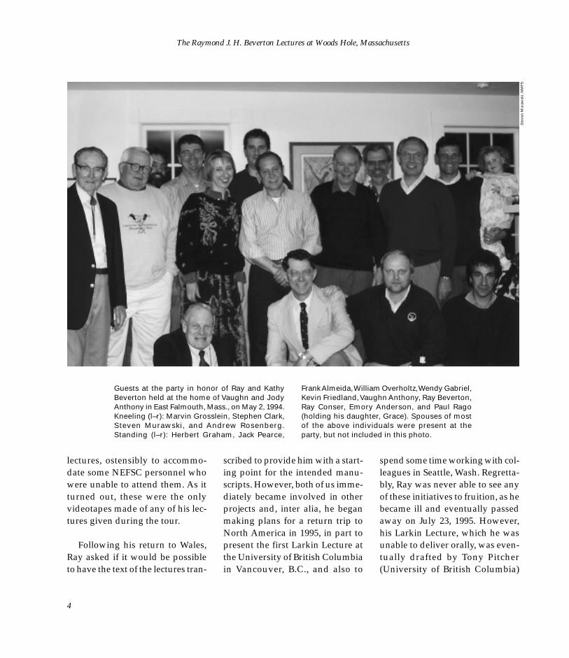
Guests at the party in honor of Ray and Kathy Beverton held at the home of Vaughn and Jody Anthony in East Falmouth, Mass., on May 2, 1994. Kneeling (l–r): Marvin Grosslein, Stephen Clark, Steven Murawski, and Andrew Rosenberg. Standing (l–r): Herbert Graham, Jack Pearce,
Frank Almeida, William Overholtz, Wendy Gabriel, Kevin Friedland, Vaughn Anthony, Ray Beverton, Ray Conser, Emory Anderson, and Paul Rago (holding his daughter, Grace). Spouses of most of the above individuals were present at the party, but not included in this photo.
lectures, ostensibly to accommodate some NEFSC personnel who were unable to attend them. As it turned out, these were the only videotapes made of any of his lectures given during the tour.
Following his return to Wales, Ray asked if it would be possible to have the text of the lectures tran
scribed to provide him with a starting point for the intended manuscripts. However, both of us immediately became involved in other projects and, inter alia, he began making plans for a return trip to North America in 1995, in part to present the first Larkin Lecture at the University of British Columbia in Vancouver, B.C., and also to
spend some time working with colleagues in Seattle, Wash. Regrettably, Ray was never able to see any of these initiatives to fruition, as he became ill and eventually passed away on July 23, 1995. However, his Larkin Lecture, which he was unable to deliver orally, was eventually drafted by Tony Pitcher (University of British Columbia)
4

Preface
and Terrance Iles (University of Wales), from detailed speaking notes that Ray had prepared, and published in 1998 as the lead pa-per in the Beverton and Holt Jubilee Special Issue of Reviews in Fish Biology and Fisheries1.
It was not until after his death that I decided to undertake the project of preparing Ray’s lectures for publication. What initially began as a full-time effort on my part to transcribe the lectures and quickly produce a set of manuscripts gradually grew into a much more difficult and painstaking task than I had ever imagined. Further-more, as other duties increasingly demanded more and more of my time and energy, the project evolved largely into a “spare-time” endeavor and ultimately took far longer than originally intended.
In contrast to the tedium of hours and hours of listening to tapes and trying to decipher each and every word was the sheer plea-sure of listening over and over to Ray’s presentations. On each occasion when I was able to devote time to working on the transcription, it was so enjoyable to again hear his voice. Each time I replayed a particular section to try to clarify what Ray had said (the audio portion of the videotapes was not of high
1Beverton, R. 1998. Fish, fact and fantasy: a long view. Rev. Fish Biol. Fish. 8:229–249.
quality), I seemed to pick up an additional nuance or meaning. Every effort was made to retain the exact words used by Ray so as to retain the distinctive “Bevertonian” delivery, while making minimal changes primarily to provide a more “reader-friendly” description of figures. The question-and-answer sessions following each lecture, which provided a further opportunity for Ray to elaborate on a variety of topics, are included in full.
The main purpose in publishing this set of lectures was to record and preserve for future reading and reference some of the accumulated wisdom, ideas, hypotheses, and recollections acquired over a distinguished career by one of the most influential, respected, and beloved fishery scientists of the 20th century. In addition, this publication constitutes my personal tribute and memorial to a unique and humble man who endeared himself to every person who had the good fortune of crossing paths with him either professionally or otherwise. This was a labor of love and served, in part, to convey some small measure of thanks and appreciation for the friendship and many kindnesses which Ray and Kathy bestowed on me and my wife over the years.
Everyone who knew Ray counted him as a genuine friend,
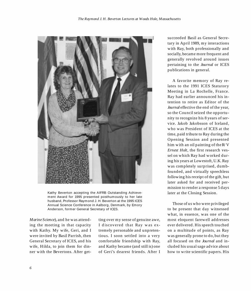
and the loss we all felt at his passing is reflected in the extraordinary number of in-depth, heartfelt, and well-deserved complimentary obituaries published worldwide in various scientific journals, newspapers, and trade magazines, the con-tents of which I will not attempt to review or emulate here. In addition, several professional fisheries societies honored Ray by bestowing upon him posthumously their highest achievement awards. These included the Silver Medal of the Fisheries Society of the British Isles and the Outstanding Achievement Award of the American Institute of Fishery Research Biologists, both conferred in 1995 and presented to his widow, Kathy. I personally had the honor of presenting the latter award to Kathy during the Opening Session of the 1995 Annual Science Conference of the International Council for the Exploration of the Sea (ICES) on September 21, 1995 in Aalborg, Den-mark.
Although I first heard of Ray Beverton in 1965 when I entered graduate school at the University of Minnesota, I do not recall actually meeting him until 1987. The occasion was the ICES Statutory Meeting (now called the Annual Science Conference) held in Santander, Spain. At the time, I was ICES Statistician and Ray was Editor of the ICES Journal du Conseil (now called the ICES Journal of
5
The Raymond J. H. Beverton Lectures at Woods Hole, Massachusetts
Kathy Beverton accepting the AIFRB Outstanding Achievement Award for 1995 presented posthumously to her late husband, Professor Raymond J. H. Beverton at the 1995 ICES Annual Science Conference in Aalborg, Denmark, by Emory Anderson, former General Secretary of ICES.
Marine Science), and he was attend- ting over my sense of genuine awe, ing the meeting in that capacity I discovered that Ray was ex-with Kathy. My wife, Geri, and I tremely personable and unpretenwere invited by Basil Parrish, then tious. I soon settled into a very General Secretary of ICES, and his comfortable friendship with Ray, wife, Hilda, to join them for din- and Kathy became (and still is) one ner with the Bevertons. After get- of Geri’s dearest friends. After I
ICE
S
succeeded Basil as General Secretary in April 1989, my interactions with Ray, both professionally and socially, became more frequent and generally revolved around issues pertaining to the Journal or ICES publications in general.
A favorite memory of Ray relates to the 1991 ICES Statutory Meeting in La Rochelle, France. Ray had earlier announced his intention to retire as Editor of the Journal effective the end of the year, so the Council seized the opportunity to recognize his 8 years of service. Jakob Jakobsson of Iceland, who was President of ICES at the time, paid tribute to Ray during the Opening Session and presented him with an oil painting of theR/V Ernest Holt, the first research vessel on which Ray had worked during his years at Lowestoft, U.K. Ray was completely surprised, dumb-founded, and virtually speechless following his receipt of the gift, but later asked for and received per-mission to render a response 5 days later at the Closing Session.
Those of us who were privileged to be present that day witnessed what, in essence, was one of the most eloquent farewell addresses ever delivered. His speech touched on a multitude of points, as Ray was generally prone to do, but they all focused on the Journal and included his usual sage advice about how to write scientific papers. His
6
Preface
closing remarks, which to me high-lighted his farewell, consisted of some light-hearted “Advice to Prospective Contributors to the ICES Journal of Marine Science,” conveyed as a parody of the final verse of Rudyard Kipling’s poem “If.” Ray and Kathy had lovingly and cleverly crafted the words in their hotel room the previous evening. A full account of his address and the parody are contained, incidentally, in the “ICES Annual Report 1991.” However, what impressed and touched me deeply that day and has remained with me ever since is that the final verse of the original poem by Kipling really speaks about Ray and his approach to life. In fact, the verse, as follows, was read by one of his grand-daughters at his funeral service on July 31, 1995:
“If you can talk with crowds and keep your virtue,
Or walk with kings— nor lose the common touch,
If neither foes nor loving friends can hurt you,
If all men count with you, but none too much;
If you can fill the unforgiving minute
With sixty seconds’ worth of distance run,
Yours is the earth and everything that’s in it,
And—which is more— you’ll be a Man, my son!”
I am indebted to a number of individuals who assisted in large or small measure with this project. Most importantly, Kathy Beverton granted permission to undertake this task and kindly supplied all of the notes, slides, original figures or drawings, and other materials which she could find in Ray’s files pertaining to the lectures. Terrance Iles, a colleague of Ray’s at the University of Wales, assisted Kathy in searching Ray’s files for hard-to-find items and answered various questions. John Ramster from Lowestoft, who had worked closely with Ray on the editorial team of the ICES Journal of Marine Science, was particularly helpful in providing the photographs used as figures in the third lecture and in answering a number of questions. Others at Lowestoft who helped or advised, particularly in tracking down literature citations, were David Cushing, Bob Dickson, David Garrod, John Pope, and Sarah Turner. Henrik Sparholt and Judith Rosenmeier in the ICES Secretariat assisted in locating a literature citation and several figures. Tore Jacobsen (Institute of Marine Research, Bergen, Norway) and Steven Murawski and Mark Terceiro (NEFSC, Woods Hole)
provided special assistance in clarifying information on Figure 31 of the first lecture. Murawski, William Overholtz, Fred Serchuk, Jackie Riley, and Jorge Csirke also helped with some literature citations. Brenda Figuerido made 8.5 × 11-inch reproductions from the 35-mm slides used by Ray in giving the lectures that were used in pre-paring many of the figures in this publication. Malcom Silverman videotaped the lectures. My wife, Geri, assisted in transcribing the audio portion of the videotapes onto Dictaphone tapes to facilitate my efforts to record in writing the full text of the lectures and all the question-and-answer sessions. Last of all, I owe a huge debt of gratitude to David Stanton of the NMFS Scientific Publications Office (SPO) in Seattle for the monumental task of reproducing, from assorted drawings, handmade sketches, and graphs, most of the figures included in this book, for the layout of the book, and for all of the interactions with the Government Printing Office. SPO Chief Willis Hobart provided editorial assistance. The NMFS Office of Science and Technology in Silver Spring, Md., provided the funding for this publication.
Emory D. AndersonEditorSilver Spring, Md.May 2002
7

“Man or Nature
in Fisheries Dynamics:
Who Calls the Tune?”
LECTURE 1
May 2, 1994
Redfield AuditoriumWoods Hole Oceanographic Institution


Ladies and Gentlemen. I am Emory Anderson, and on behalf of the NMFS North-
east Fisheries Science Center, as well as the Woods Hole Oceanographic Institution and the Marine Biological Laboratory, who have graciously provided auditorium facilities, it is my pleasure to welcome you to the first of three lectures to be presented today and to-morrow by a very distinguished European guest. I might add that our guest is starting a nationwide lecture tour here today that will continue in Seattle, Wash.; Auke Bay, Alaska; La Jolla, Calif.; and Beaufort, N.C.; and then conclude in about 3 weeks in Silver Spring, Md., the headquarters of the National Marine Fisheries Service. This tour is sponsored by the National Marine Fisheries Service.
Our guest is one of the world’s preeminent fisheries scientists whose name is synonymous with quantitative fisheries science. He was educated at Cambridge University, received his M.A. degree with first class honors in zoology in 1947, and in that year joined the staff of the Fisheries Laboratory in Lowestoft as a research officer. However, as he told me, he actually started working there briefly in 1945 after the war, but then went on to Cambridge to finish his degree. Together with colleague Sidney Holt, he authored the classic 1957 monograph entitled “On
the Dynamics of Exploited Fish Populations” (Beverton and Holt, 1957) which, perhaps more than any other single contribution, has defined and described the theoretical and quantitative basis for fish stock management. The results of that work are still as relevant to-day as they were 40 years ago. The familiar “Beverton and Holt yield-per-recruit” concept constitutes only a small part of that master-piece.
Ray remained in Lowestoft for 18 years, leaving in 1965, having served as Deputy Director since 1959. During those years, he was a very energetic proponent of the use of quantitative methods for providing a sound scientific basis for the management and rational exploitation of fisheries resources. As such, he was very active in inter-national fisheries work in the North Atlantic under the auspices of organizations such as the Inter-national Council for the Exploration of the Sea (ICES) and the International Commission for the Northwest Atlantic Fisheries (ICNAF).
In 1965, he assumed the post of Secretary and Chief Executive of the newly formed U.K. Natural Environment Research Council (NERC) which was the principle U.K. funding source for nongovernmental life science and environmental research. The NERC was re
sponsible then and until recently for directing the activities of, for ex-ample, the British Geological Survey, the British Antarctic Survey, and the well known Continuous Plankton Recorder survey.
In the early 1980’s, following mandatory retirement from NERC, Ray ventured into the academic arena and returned to a more direct involvement in fisheries re-search, first at the University of Bristol as a Senior Research Fellow, and later at the University of Wales, Cardiff, where he became Professor of Fisheries Ecology in 1984. From 1987 to 1989 he was Head of the School of Pure and Applied Biology and then, again because of reaching another mandatory retirement age, he was obliged to retire a second time. Since 1990, Ray has been Professor Emeritus at the University of Wales, but he has continued to lecture (giving the only fisheries course there), write papers, and provide advice to students. To say that he had retired is really a misnomer of the first order.
Since the early 1980’s, Ray has held positions of leadership in a number of societies, committees, and organizations including President of the Fisheries Society of the British Isles, Vice President of the Freshwater Biological Association, Head of the U.K. Delegation to the Intergovernmental Oceanographic Commission (IOC), and President
11
The Raymond J. H. Beverton Lectures at Woods Hole, Massachusetts
of the Challenger Society for the Advancement of Marine Science, just to name a few. I might also point out that Ray is a recipient of several very prominent awards, including Commander of the British Empire in 1968, Fellow of the Institute of Biology in 1973, Fellow of the Royal Society in 1975, Honorary Doctorate of Science from the University of Wales in 1989, and most recently, which some of you in this room witnessed in August 1993, the American Fisheries Society Award of Excellence.
As author of innumerable scientific papers, Ray established a very high standard in the art of de-scribing, in writing, the results of scientific inquiry. It was perhaps only natural, then, that in 1983 he was asked to assume the post of Editor of ICES’ premiere publication, the Journal du Conseil (now called the ICES Journal of Marine Science). In that capacity, and with the assistance of his good wife, Kathy, he singlehandedly restored the quality and reputation of this prestigious journal. While serving as Editor until the end of 1991, he gained the respect of many young authors for his willingness to work with them to improve their manuscripts to acceptable standards. I think it is fair to say that this at-tribute is not universally shared by many journal editors. When I was General Secretary of ICES, I had the good fortune to interact with Ray
in his capacity as Editor and to be-come personally acquainted with him.
As university students and then as fish stock assessment scientists, many of us have for years been in awe of this man and his achievements in fish population dynamics. But in spite of his brilliance, in spite of having had such a pro-found impact on his profession and on the discipline of a magnitude that few others can claim, and de-spite being a recipient of so many accolades, he is still a very down-to-earth, enthusiastic, likeable, friendly person, which is why he has endeared himself to so many of us.
We are indeed fortunate to have such a stalwart with us today and to be privileged to hear him speak on the topic “Man or Nature in Fisheries Dynamics: Who Calls the Tune?” Please join me in welcoming Professor Ray Beverton.”
Ray Beverton Emory, Ladies and Gentlemen.
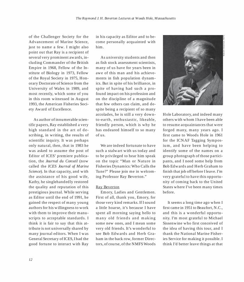
First of all, thank you, Emory, for those very kind remarks. If I sound a little hoarse, it’s because I have spent all morning saying hello to many old friends and making some new ones, and I mean some very old friends. It’s wonderful to see Bob Edwards and Herb Graham in the back row, former Directors, of course, of the NMFS Woods
Hole Laboratory, and indeed many others with whom I have been able to resume acquaintances that were forged many, many years ago. I first came to Woods Hole in 1961 for the ICNAF Tagging Symposium, and have been helping to identify some of the names on a group photograph of those participants, and I need some help from Bob Edwards and Herb Graham to finish that job off before I leave. I’m very grateful to have this opportunity of coming back to the United States where I’ve been many times before.
It seems a long time ago when I first came in 1951 to Beaufort, N.C., and this is a wonderful opportunity. I’m most grateful to Michael Sissenwine who first conceived of the idea of having this tour, and I thank the National Marine Fisheries Service for making it possible. I think I’d better leave things at that
Mal
colm
Silv
erm
an, N
MFS
12
Lecture 1: Man or Nature in Fisheries Dynamics: Who Calls the Tune?
point to get on with the substance of my talk because there is quite a lot I want to try and say in a relatively short time. Incidently, I also want to thank Brenda Figuerido for getting last-minute slides done for me which I couldn’t get through in time before I left.
The subject of today’s talk, “Man or Nature in Fisheries Dynamics: Who Calls the Tune?” was chosen because I felt that this is a dilemma, a polarization of approaches, attitudes, and evidence that has been with us right from the beginning. You’ve only got to turn the clock right back to the beginning of ICES at the turn of the century, and there you find the Scandinavian lobby, the Norwegians in particular, pressing for studies in fluctuations1 because they had been used to knowing what it is like to have a fishery that was highly fluctuating, which I will tell you more about in a moment.
1This led to the establishment of an ICES Committee on Migration of Food Fishes, headed by Johan Hjort of Norway.
Mal
colm
Silv
erm
an, N
MFS
The other committee [the second of the three ICES Committees established initially] that was set up was, in effect, on the overfishing problem in the North Sea, which was perceived quite clearly even in those days. This Commit-tee was headed initially by Walter Garstang, who founded the Lowestoft Lab in 1902, and later by Friedrich Heincke who took it over from him. So there were the initial steps, but they were running in parallel in those days, and it wasn’t too difficult to keep the two lines of approach separate. Of course, the first one led to Johan Hjort’s classic paper [on the great fisheries fluctuations of northern Europe] (Hjort, 1914). The Commit-tees reported in 1913 and 1914, each with very important monographs, of which Hjort’s is possibly the better known, but Heincke’s (1913) was equally important.
But nowadays, of course, we’ve got much more complicated situations. We’ve got both fishing and nature’s influence going hand in hand, and the problem of how to disentangle these, how much of a given change or lack of change is being due to one or other factor. How to unravel their joint action or effect is no trivial problem. And it pervades all our thinking just as much now as it did a hundred years ago. And I expect you will find, if you talk to your colleagues, some of them are much more con
cerned with the oceanographic side of things and others with the fisheries side, so you will still get tendencies of, well, “Most of it’s due to big influences and climate and all the rest of it,” while others will say, “No, the fisheries has re-ally been the thing that really made the profound impact.”
So I’m going to see if I can just lead you gently through a little bit of this undergrowth in the hope that, at the end of it, we can per-haps get at least some idea of how it is possible to unravel, to a certain extent, these complicated interactions. Tomorrow’s lecture will be looking down to the individual fish and asking how they can respond, in terms of their lifestyle and their reproductive strategies, to the sort of changes, natural and manmade, that are imposed on them.
Let’s get started then. I think it might be appropriate, since I am in the area of the Pilgrim Fathers, to show you a little example where, for once, it is possible (because almost certainly the influence of fishing was very trivial in those days) to go back to the 1600’s and see an alternating act between two spe-cies2, herring and pilchard in the U.K.’s West Channel, and it gives
2Scientific names of the fishes referred to in this book are given in Appendix I.
13

The Raymond J. H. Beverton Lectures at Woods Hole, Massachusetts
LUXEMBOURG
SWITZERLAND
SHETLAND ISLANDS
ORKNEY ISLANDS
Falmouth
VIa
VIIb
VIIj
IVa
VIIg
VIIh VIIe
VIIIa
VIId
VIIa
IVb
IVc
IIIa
60A W
11A W
9A W
12A W
5 AW
55A N
60A 30´ N
52A N
51A N
50A 30´ N
49A 30´ N
48A N
47A N
7A W
57A 30´ N
53A 30´ N
IIIc IRELAND
UNITED KINGDOM
BELGIUM
FRANCE
GERMANY
DENMARK 20
0m
1000
m
2500
m
1000
m
200m
47A 30´ N
5A W
VIIf
HEBRIDES
7A E
8A E
200m
CELTIC
SEA
NORTH
SEA
1000
m
Plymouth
NET
HERLA
NDS
NORWAY
VIb
VIIc
VIIk
15A W
18A W
54A 30´ N
52A 30´ N
1000m
Figure 1. Map showing the western approaches to the United Kingdom and Ireland, with surrounding water bodies delineated as ICES statistical areas.
you a little confidence that indeed you can see some effects without having to worry too much about the complexities of extrapolations.
In Figure 1, Plymouth and Falmouth are in the southwest corner of the U.K., so that locates you with two names you are very familiar with. The oceanography of this
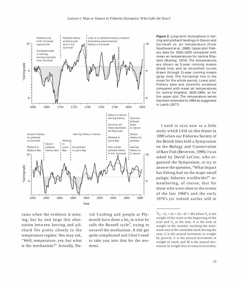
area is dominated by a front that appears between essentially the Gulf Stream, with its meanderings and sawtooths going up to the north, and the more reserved water that eventually finds its way to the North Sea. People at Plymouth, not so long ago, unearthed the his-tory of this right back to 1660 (Fig. 2) with a sufficient temperature
record to follow it. The shaded areas are where the temperature is below the long-term norm, and the unshaded areas are above. You can see, in general, the herring was strong, in terms of the fishing activity, when the temperatures were below normal, and the pilchards took over when the temperature was above. There are one or two
14
Lecture 1: Man or Nature in Fisheries Dynamics: Who Calls the Tune? AC
enti
gra
de
ACen
tig
rad
e
Pilchard only in W. Cornwall; exports low
Increased trade in herring; herring exported from Cornwall
Pilchard fishery at Dartmouth and in S.E. Cornwall
Little or no pilchard fishery in Devon; fluctuating autumn/winter fishery in Cornwall
Pilc
har
d f
ish
ery
po
or
9
8
1660 1680 1700 1720 1740 1760 1780 1800 1820
10
9
Autumn fishery for pilchard in Cornwall
Pilchard in Bigbury Bay
Devon pilchard fishery fails
Pilchard in Lyme Bay
No pilchard in Lyme Bay
Herring fishery in Devon
Failure of Devon herring fishery
Summer pil-chard abundant off Plymouth
Pilchard in Lyme Bay
Poor winter pilchard fishery in S.E. Cornwall
Summer pilchard leave S. Devon
Winter fishery for pilchard
Herring fishery in E. Devon
1820 1840 1860 1880 1900 1920 1940 1960 1980
Year
Figure 2. Long-term fluctuations in her-ring and pilchard landings in Devon and
10 10 Cornwall vs. air temperature (fromSouthward et al., 1988). Upper plot: Fishery data for 1650–1820 compared withmean air temperatures for central England (Manley, 1974). The temperaturesare shown as 5-year running means
9
8
10
9
(black line) and as smoothed curves drawn through 11-year running means (gray line). The horizontal line is the mean for the whole period. Lower plot: Fishery data and scientific evidence compared with mean air temperatures for central England, 1820–1984, as for the upper plot. The temperature series has been extended to 1984 as suggested in Lamb (1977).
I need to turn now to a little study which I did on this theme in 1990 when our Fisheries Society of the British Isles held a Symposium on the Biology and Conservation of Rare Fish (Beverton, 1990). I was asked by David LeCren, who organized the Symposium, to try to answer the question, “What impact has fishing had on the major small pelagic fisheries worldwide?” remembering, of course, that for those who were close to the events of the late 1960’s and the early 1970’s (or indeed earlier still in
3S2 = S1 + (A + G) – (C + M) where S1 is the weight of the stock at the beginning of the year and S2 at the end, A is the sum in weight of the number reaching the mini-mum size of the catchable stock during the year, G is the annual increment in weight by growth, C is the annual decrement in weight of catch, and M is the annual decrement in weight due to natural mortality.
cases when the evidence is missing, but by and large this alter-nation between herring and pilchard fits pretty closely to the temperature regime. You may ask, “Well, temperature, yes, but what is the mechanism?” Actually, Da
vid Cushing and people at Ply-mouth have done a lot, in what he calls the Russell cycle3, trying to unravel the mechanism. It did get quite complicated and I don’t need to take you into that for the moment.
15

The Raymond J. H. Beverton Lectures at Woods Hole, Massachusetts
kcotS
kaeP despalloC
leuqeS
raeY tludA 01.son 9 raeY
tludA .son 01 9
noitcarF kaepfo
-gnirpsnaigewroN gnirrehgninwaps
7591 04 2791 61.0 052/1 ;sraey01retfayrevocerdetimiL
ssalcraey3891notnedneped x
-gnirpscidnalecI gnirrehgninwaps
7591 3 2791 100.0 0003/1 2891ecnisngisoN
-remmuscidnalecI gnirrehgninwaps
1691 1 2791 30.0 03/1 dedrocertsehgihotyrevocergnortS
level
aeShtroNnrehtuoS gnirreh
9491 5.2 6791 10.0 003/1 tuobaotyrevocergnortsyletaredoM t
fo4/1 f kaep xx
gnirrehknaBsegroeG 7691 5 6791 ylbaborp
10.0< ylbaborp
005/1< ;48–7791deraeppasidyllautriV
ylgnortsylriafgnirevocerwon
enidrasainrofilaC 9491 3 5691 )5791(
510.0 )10.0(
052/1 )057/1(
-erpavraltub,yrehsifonhtiwsraey02 5891ecnisyrevocergnortsylriaf;tnes xx
drahclipnacirfAhtuoS 0691 5.4 2891 60.0 07/1 2891ecnisyrevocerwolS
atevohcnanaivureP 2691 005 3791
28–0891 52 52
02/1 02/1
;sraeyoñiNlEerew2891dna2791 kaepotkcabtontub,yrevocerdipar xx
nilepacaeSstneraB 1891 53 6891 3.0 001/1 skcotstub,6891ecnisgnihsifoN
yldipargnirevocer
lerekcamcificaP 3391 1 8691 300.0 003/1 ;5791dna8691neewtebsdroceroN
eziskaep2/1otyrevocerdiparneht x
Figure 3. Collapses of various marine pelagic fisheries.
California), the memory of some of those very dramatic collapses is only too fresh. So I thought, “Well, that’s an interesting one; we’ll have a look and see what can be done.”
Somewhat to my surprise, what didn’t seem too promising at the time turned into a very systematic study. I got out a list of the ten best documented examples (Fig. 3) of
what I could call pretty serious fishery collapses, right down to 1/20 or less of their peak abundance. The first five are herring, and the first three of those are the Atlanto-Scandian (which I shall go into more detail in a moment), south-ern North Sea, and Georges Bank. Then come some related species (not herring): the California sardine, South African pilchard, Peru
vian anchoveta (of course, that’s the El Niño story), Barents Sea capelin, and Pacific mackerel.
These species all had boom years around about 1950 and 1960, and then collapsed at the end of the 1960’s or early 1970’s. Some went right down to a very small fraction of their peak abundance. The final story, which we can pick up later,
16
Lecture 1: Man or Nature in Fisheries Dynamics: Who Calls the Tune?
NM
FS
is that in all but one case, they hung on, as it were. They persisted, of-ten at very low levels, and eventually, to some degree or other (in one or two cases very substantially), notably right on your doorstep here on Georges Bank, they have come back with a bang. But one, the Icelandic spring-spawning her-ring, didn’t, and we’ll have a look at that in a moment.
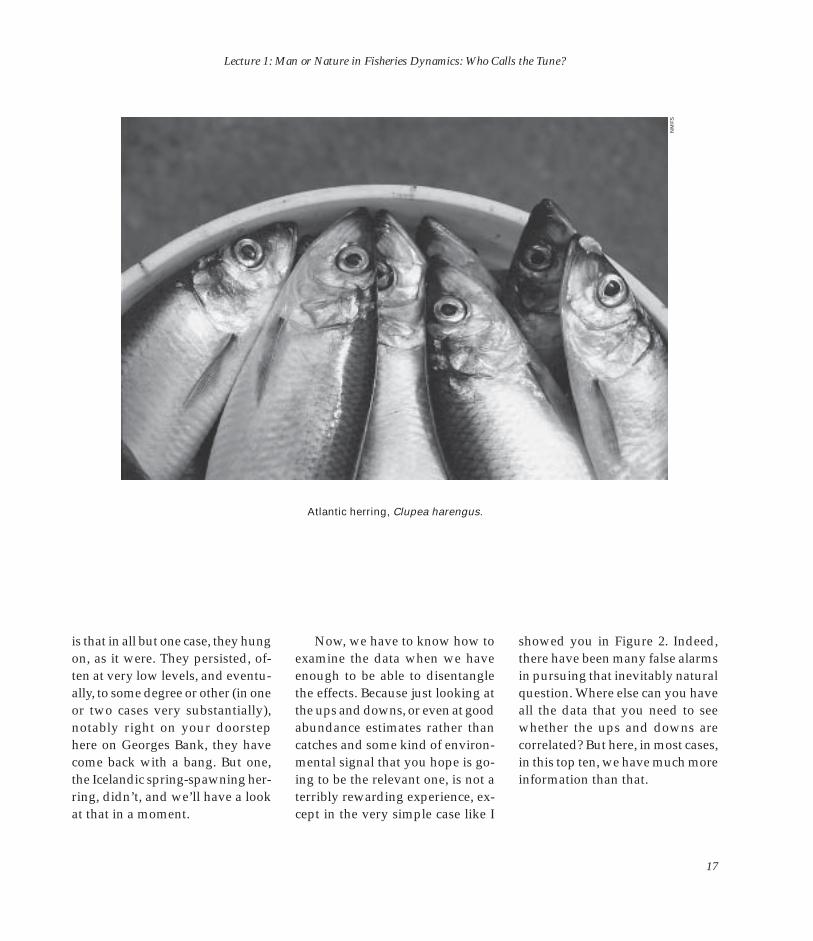
Atlantic herring, Clupea harengus.
Now, we have to know how to examine the data when we have enough to be able to disentangle the effects. Because just looking at the ups and downs, or even at good abundance estimates rather than catches and some kind of environmental signal that you hope is going to be the relevant one, is not a terribly rewarding experience, except in the very simple case like I
showed you in Figure 2. Indeed, there have been many false alarms in pursuing that inevitably natural question. Where else can you have all the data that you need to see whether the ups and downs are correlated? But here, in most cases, in this top ten, we have much more information than that.
17

The Raymond J. H. Beverton Lectures at Woods Hole, Massachusetts
S/R decreasing A
R/S decreasing
B
R R
S S
R
R
S
R/S
Time
S
C
E
R
S S
Time
R/S R/S
S S
Time Time
R
S
D
R/S
S
F
Let me just remind you of the way you need to analyze the situation when you have these estimates of stock and recruitment as in Figure 4. If you have stock size on the bottom and recruitment up the side (Fig. 4A), and if you have a situation in which the survival to recruitment from the stock is given by the curve there, and any of the straight lines is the other way around, that is the stock produced throughout the subsequent lifetime giving you recruitment, and where those two lines cross is the stable point. If they don’t cross, then the population is either in the process of declining or expanding.
If fishing pressure increases (Figs. 4A, C, E), then the steepness of those lines increases because the amount of stock which a given recruitment can produce becomes less and less. If it gets to the point at which it doesn’t intercept that curve anymore, then the population is heading for its graveyard. How long it takes to get there will depend, of course, upon fluctuations and various things, but sooner or later, it is technically in an unstable state.
Figure 4.Theory of collapse as described by stock-recruitment relationships, with A, C, and E illustrating the effects of in-creasing fishing pressure and B, D, and F representing the effects of environmental impacts.
18

Lecture 1: Man or Nature in Fisheries Dynamics: Who Calls the Tune?
NM
FS
The symptoms, therefore, indicate (if that’s what’s happened to a stock) that this is a fishing generated event, and then the stock will fall as this goes across that way. It will initially stay up pretty well, depending on how flat-topped the curve is, but eventually it will start to plummet quite radically (Fig. 4C). A particularly valuable index is, in effect, the reproductive rate (recruitment rate per parent or R/S) which increases steadily through-out (Fig. 4E), because on that shape of curve, the recruitment rate (the proportion of the recruitment over stock), the survival rate is improving all the way as the stock falls. So in time, the recruitment rate goes up as the stock falls.
The British herring fleet departing at daybreak.
Now, the other way around is when it’s an environmentally mediated event (Fig. 4B, D, F), especially if it’s an event that is affecting the early life history, and most are. It’s a bit of a simplification to take that as the only way it can hap-pen, but it’s the general way. Then, fishing pressure stays the same, but the survival curve would gradually decrease and you’d get fewer recruits from a given stock. And so there will be a series of stable points (Fig. 4B), falling possibly, if the survival rate’s going faster than that, you might even come down the right side. The effect of that is that the stock still declines as be-fore, but the recruitment falls also initially and at roughly the same
rate (Fig. 4D). Whereas, in particular, the recruitment success rate, in-stead of going up all the time, actually is either staying constant or even possibly declining slightly as the population attempts to stabilize itself on the way down (Fig. 4F).
I’m sorry about that little bit of an explanation, but I think we need that in order to examine, therefore, these top ten stocks in terms of what happened, the time sequence of stock abundance and recruitment success rate as time went by.
19

The Raymond J. H. Beverton Lectures at Woods Hole, Massachusetts
Log
eR
/S
Log
eR
/SLo
ge
R/S
Figure 5. Plots of spawning stock biomass (SSB) and the natural logs of recruitment/stock (R/S) for stocks of Atlanto-Scandian herring: Norwegian spring-spawning herring (A), Icelandic spring-spawning her-ring (B), and Icelandic summer-spawning herring (C).
In each part of Figure 5, the stock size is the heavy gray curve and years are along the bottom, starting back in 1945 right up to the 1990’s as near as I can get it. The heavy gray curve is the stock size, and the black dots are the recruitment rate [R/S] calculated year by year. The shaded area is where the fishing pressure has exceeded the capacity of the recruitment rate at that moment to replenish itself. In other words, the recruitment rate would have to go up to the top of the shaded areas to be able to compensate, over the lifetime of those recruits, for the depletion, caused by fishing, of the spawning stock. It’s a little bit of a problem because recruitment rate happens year by year and these are the other way around. It’s a long-term projection, but it’s an unavoidable problem with this kind of data, and it’s the simplest way of indicating whether the reproductive rate, the recruitment success rate, is able to keep up with or compensate for the depletion.
Now, in the case of the Norwegian spring-spawning herring (Fig. 5A), the answer was that as the population fell, especially when it got down to the extreme low level in the early 1970’s [A], the recruitment rate went up quite markedly. Fishing was stopped in about 1973, but then as the population recovered a bit, it [recruitment rate] came down very substantially, much
1945 1950 1955 1960 1965 1970 1975 1980 1985
4
3
2
1
0
–1
Norwegian spring-spawning herring
SS
B (10
–9 kg)
A
5
6
7
8
–2
4
3
2
1
0
5
6
7
8
9
10
B
4
3
2
1
0
–1
5
–2
–3
–4 1945 1950 1955 1960 1965 1970 1975 1980 1985
4
3
2
1
0
5
6
7
8
9Icelandic spring-spawning herring
A
4
3
2
1
0
–1
–2 1945 1950 1955 1960 1965 1970 1975 1980 1985
Icelandic summer-spawning herring
A
4
3
2
1
0
5
6
SSB
R/S
R/S
SSB
SSB
R/S
SS
B (10
–8 kg)
SS
B (10
–8 kg)
(R/S)0
(R/S)0
(R/S)0
A
B
C
Year
20
Lecture 1: Man or Nature in Fisheries Dynamics: Who Calls the Tune?
Alle
n S
him
ada,
NM
FS
more than you would have expected it to, and except for one blip [B], which is the 1983 year class, it stayed rather disappointingly down. As a result, the recovery of the Norwegian springs has been very slow.
The Icelandic spring-spawning herring is a real boom-bust story (Fig. 5B). It came from very small beginnings and then faded away,
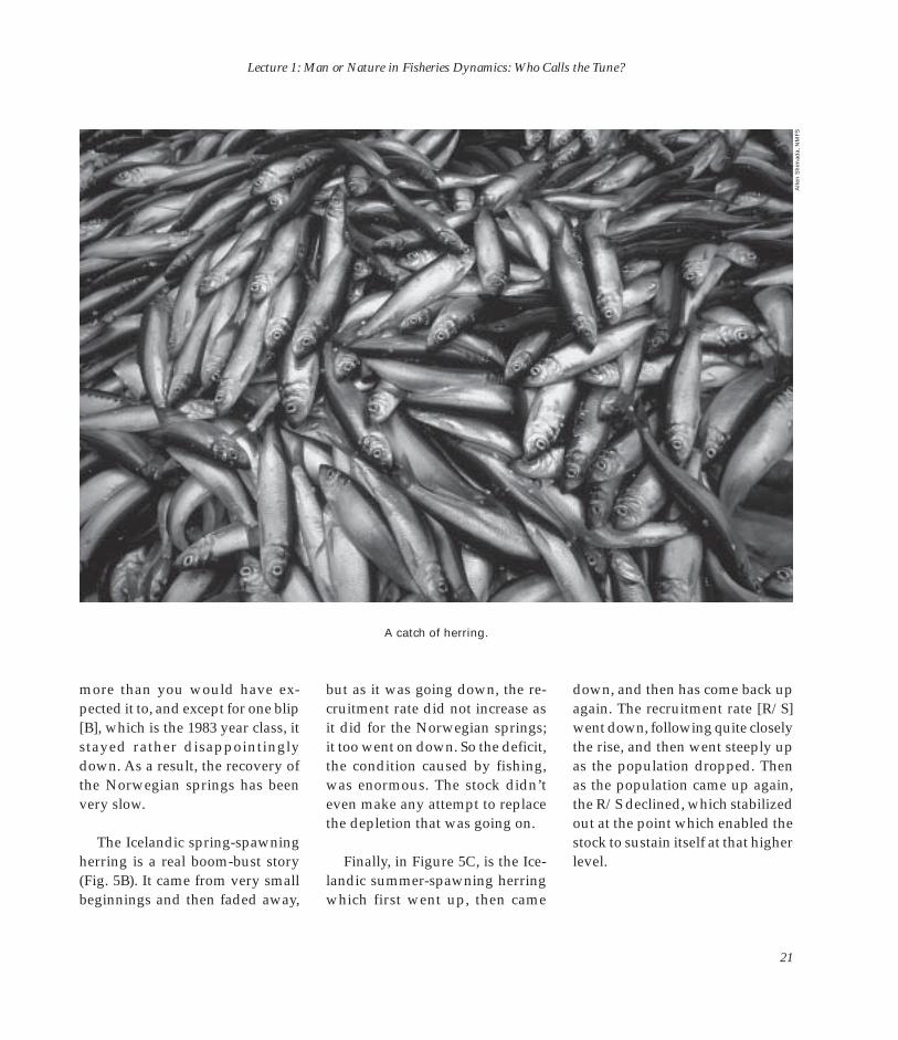
A catch of herring.
but as it was going down, the recruitment rate did not increase as it did for the Norwegian springs; it too went on down. So the deficit, the condition caused by fishing, was enormous. The stock didn’t even make any attempt to replace the depletion that was going on.
Finally, in Figure 5C, is the Icelandic summer-spawning herring which first went up, then came
down, and then has come back up again. The recruitment rate [R/S] went down, following quite closely the rise, and then went steeply up as the population dropped. Then as the population came up again, the R/S declined, which stabilized out at the point which enabled the stock to sustain itself at that higher level.
21

The Raymond J. H. Beverton Lectures at Woods Hole, Massachusetts
Southern North Sea herring
A B
SSB R/S
(R/S)0
ANow, the next two figures are on 4 5
this same topic, which I won’t have 3 4
time to go into detail, but I’ll just 2 3
run through very quickly just to 1 2
show you that the same kind of 0 1
patterns can be found in the vari- –1 0
ous others. That’s the southern 1945 1950 1955 1960 1965 1970 1975 1980 1985
North Sea herring (Fig. 6A) where 1.5
it went down and stayed down 3
over a long period. The reproduc-2
Georges Bank herring
SSB
R/S
(R/S)0
B 1
tive rate did increase, especially in 1the end, and they were able to
bounce back fairly well. Georges 0 0.5
Bank herring (Fig. 6B) was very –1
much like the Icelandic springs in –2 1945 1950 1955 1960 1965 1970 1975 1980 1985
0
the sense that, over the period, its R/S ratio did not respond to the de-clining stock. California sardines
4
3
8 7
(Fig. 6C) were dipping about for 2
6 5
some 10–20 years and finally gave
California sardine
A ?
SSB R/S
(R/S)0
C
4
up the ghost, as it were, and their1 3
0 2 reproductive rate fell off quite dra- 1
0matically toward the end, and that 1945 1950 1955 1960 1965 1970 1975 1980 1985
meant a complete collapse of the stock. Finally, the South African pil-
South African pilchard SSB
R/S
(R/S)0
D
16
chard (Fig. 6D) did respond quite 14
well to the initial decline, but then 6 12
has not responded beyond that 5 10
point. 4 8
3 6
2 4
1 2
0 0 1945 1950 1955 1960 1965 1970 1975 1980 1985
Year
Figure 6. Plots of spawning stock biomass (SSB) and the natural logs of recruitment/stock (R/S) for stocks of southern North Sea herring (A), Georges Bank herring (B), California sardine (C), and South African pilchard (D).
Log
eR
/S
Log
eR
/SLo
ge
R/S
Lo
ge
R/S
SS
B (10
–8 kg)
SS
B (10
–9 kg)
SS
B (10
–8 kg)
SS
B (10
–8 kg)
22

Lecture 1: Man or Nature in Fisheries Dynamics: Who Calls the Tune?
Finally, just to finish the top ten, the Peruvian anchovy (Fig. 7A), which of course had this very massive El Niño effect in the early 1970’s, responded up to a point, but not very dramatically so. So, it didn’t recover as well as it might have done because fishing had to be pretty drastically stopped. Barents Sea capelin (Fig. 7B) was going up and down all over the place, but that’s a story we’ll have to come to in a moment. Finally, with Pacific mackerel (Fig. 7C), again, we see a recruitment rate that was rather erratic, sometimes tracking the declining stock and sometimes not, although at the end it went up quite steeply. By this time, the depletion caused by fishing was too much for it to cope with, and it too disappeared for quite some time.
Figure 7. Plots of spawning stock biomass (SSB) and the natural logs of recruitment/stock (R/S) for stocks of Peruvian anchovy (A), Barents Sea capelin (B), and Pacific mackerel (C).
7
6
5
4
3
2 1945 1950 1955 1960 1965 1970 1975 1980 1985 1990
10
20
30Peruvian anchovetta
7
6
5
4
3
8
9
1945 1950 1955 1960 1965 1970 1975 1980 1985 1990
Barents Sea capelin
1.5
2.0
1.0
0.5
0
A
1
0
–1
–2
–3
2
3
–4
3
2
1
0
Pacific mackerel
1945 1950 1955 1960 1965 1970 1975 19801935 1940
0
SS
B (10
–9 kg)
SS
B (10
–9 kg)
SS
B (10
–8 kg)
R/S
R/S
R/S
SSB
SSB
SSB
(R/S)0
(R/S)0
(R/S)0
A
B
C
Year
Log
e R
/S
Log
e R
/S
Log
e R
/S
23

The Raymond J. H. Beverton Lectures at Woods Hole, Massachusetts
So much for that story. Now we have to look in a little more detail and concentrate on the three Atlanto-Scandian herrings: the Norwegian and the two Icelandics.
75A�
Icelandic spring and summer spawners
Spawning area
(Icelandic)
Polar front
Norwegian spring
spawners
Wintering area
Spawning area
(Norwegian)
Feed
ing
area
Feeding area
Between them, they really cover the full range of what’s happened: one disappearing completely, an-other recovering very strongly, and the third dithering about for a long time before it reappeared. Indeed,
70A� I’d just remind you that we’re talking about the area between Nor-way and Iceland (Fig. 8), the feeding area up against the polar front, a migration back for the Norweg-
65A� ians to spawn, and then starting, when they’re mature, that cycle again. The Icelandic springs and summers spawn off the southern part of the island and feed and mix
60A up with the top ones to feed in the summer. So that’s the general geography.
20A 10A 0A 10A 20A 30A
Figure 8. Distribution of stocks within the Atlanto-Scandian herring group. Redrawn from Dragesund et al. (1980), and with additional detail provided by Ray Beverton.
An early scientific illustration of a herring, showing fine detail.
24
Lecture 1: Man or Nature in Fisheries Dynamics: Who Calls the Tune?
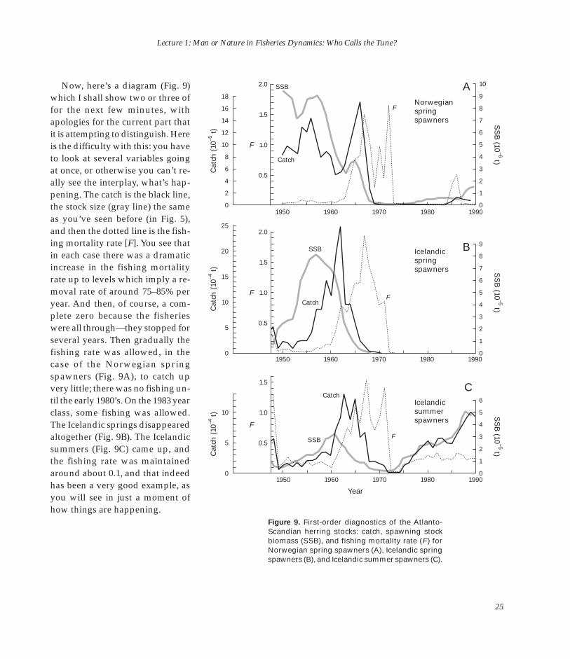
Now, here’s a diagram (Fig. 9) which I shall show two or three of for the next few minutes, with apologies for the current part that it is attempting to distinguish. Here is the difficulty with this: you have to look at several variables going at once, or otherwise you can’t re-ally see the interplay, what’s happening. The catch is the black line, the stock size (gray line) the same as you’ve seen before (in Fig. 5), and then the dotted line is the fishing mortality rate [F]. You see that in each case there was a dramatic increase in the fishing mortality rate up to levels which imply a removal rate of around 75–85% per year. And then, of course, a complete zero because the fisheries were all through—they stopped for several years. Then gradually the fishing rate was allowed, in the case of the Norwegian spring spawners (Fig. 9A), to catch up very little; there was no fishing until the early 1980’s. On the 1983 year class, some fishing was allowed. The Icelandic springs disappeared altogether (Fig. 9B). The Icelandic summers (Fig. 9C) came up, and the fishing rate was maintained around about 0.1, and that indeed has been a very good example, as you will see in just a moment of how things are happening.
Cat
ch (
10–4
t)
Cat
ch (
10–5
t)
Cat
ch (
10–4
t)
10
18 SSB 2.0
1.5
1.0
0.5
Catch
F Norwegian spring spawners
A
F
9
16 8
14 7
12 6
10 5
8 4
6 3
4 2
2 1
0 0 1950 1960 1970 1980 1990
25
9 20
8
7 15 6
5
10
SSB
Catch F
1.5
2.0
1.0
0.5
Icelandic spring spawners
B
F
4
3
5 2
1
0 0 1950 1960 1970 1980 1990
6
10
SSB
Catch
F
1.0
1.5
0.5
Icelandic summer spawners
C
F
5
4
3 5
2
1
0 0 1950 1960 1970 1980 1990
Year
Figure 9. First-order diagnostics of the Atlanto-Scandian herring stocks: catch, spawning stock biomass (SSB), and fishing mortality rate (F ) for Norwegian spring spawners (A), Icelandic spring spawners (B), and Icelandic summer spawners (C).
SS
B (10
–6 t) S
SB
(10–5 t)
SS
B (10
–5 t)
25
The Raymond J. H. Beverton Lectures at Woods Hole, Massachusetts
10
5
0 0 5 10
SSB (10–6 kg)
49
67 65
F = 1.2 (1967) F = 0.9
(1964)
F = 0.15 (1960)
F = 0.05 (1947–57)
F = 0
66
64
48 63
47
62
50
51
52
53 61
54 60
55
58
59
57
56
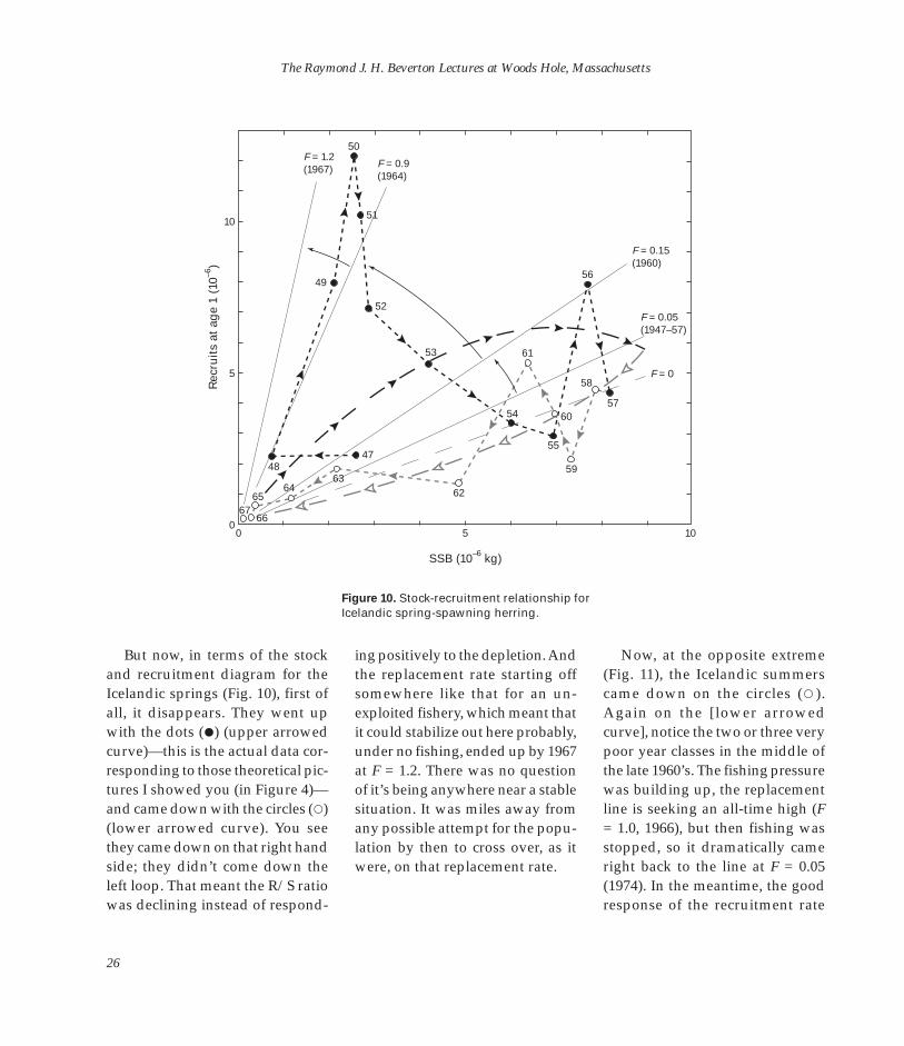
Figure 10. Stock-recruitment relationship for
Rec
ruit
s at
ag
e 1
(10–6
)
Icelandic spring-spawning herring.
But now, in terms of the stock and recruitment diagram for the Icelandic springs (Fig. 10), first of all, it disappears. They went up with the dots (�) (upper arrowed curve)—this is the actual data corresponding to those theoretical pictures I showed you (in Figure 4)— and came down with the circles (�) (lower arrowed curve). You see they came down on that right hand side; they didn’t come down the left loop. That meant the R/S ratio was declining instead of respond
ing positively to the depletion. And the replacement rate starting off somewhere like that for an unexploited fishery, which meant that it could stabilize out here probably, under no fishing, ended up by 1967 at F = 1.2. There was no question of it’s being anywhere near a stable situation. It was miles away from any possible attempt for the population by then to cross over, as it were, on that replacement rate.
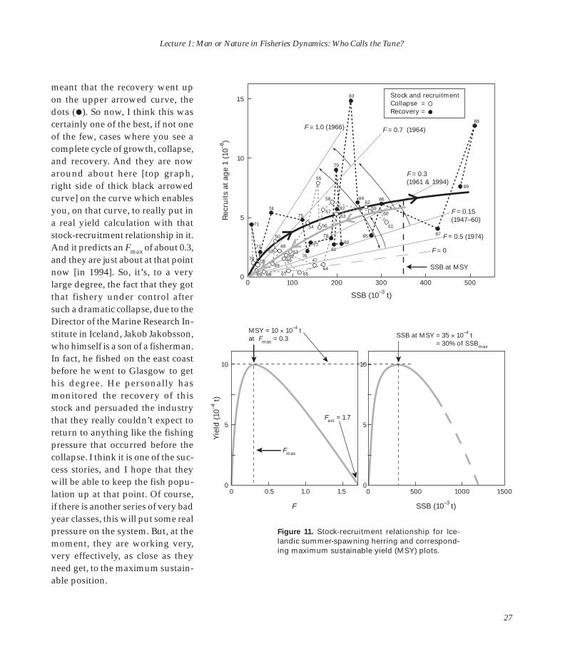
Now, at the opposite extreme (Fig. 11), the Icelandic summers came down on the circles (� ). Again on the [lower arrowed curve], notice the two or three very poor year classes in the middle of the late 1960’s. The fishing pressure was building up, the replacement line is seeking an all-time high (F = 1.0, 1966), but then fishing was stopped, so it dramatically came right back to the line at F = 0.05 (1974). In the meantime, the good response of the recruitment rate
26
Lecture 1: Man or Nature in Fisheries Dynamics: Who Calls the Tune?
meant that the recovery went up on the upper arrowed curve, the dots (�). So now, I think this was certainly one of the best, if not one of the few, cases where you see a complete cycle of growth, collapse, and recovery. And they are now around about here [top graph, right side of thick black arrowed curve] on the curve which enables you, on that curve, to really put in a real yield calculation with that stock-recruitment relationship in it. And it predicts an F max of about 0.3, and they are just about at that point now [in 1994]. So, it’s, to a very large degree, the fact that they got that fishery under control after such a dramatic collapse, due to the Director of the Marine Research Institute in Iceland, Jakob Jakobsson, who himself is a son of a fisherman. In fact, he fished on the east coast before he went to Glasgow to get his degree. He personally has monitored the recovery of this stock and persuaded the industry that they really couldn’t expect to return to anything like the fishing pressure that occurred before the collapse. I think it is one of the success stories, and I hope that they will be able to keep the fish population up at that point. Of course, if there is another series of very bad year classes, this will put some real pressure on the system. But, at the moment, they are working very, very effectively, as close as they need get, to the maximum sustain-able position.
Yie
ld (
10–4
t)
Rec
ruit
s at
ag
e 1
(10–8
)
15
10
5
0 0 100 200 300 400 500
SSB (10–3 t)
SSB at MSY
Collapse Recovery =
71
74
70 72
73 51
48
49
68 69
66
67
52 53
75
54
76
77
65
47
64
56
78
81 80
55
57
79
58
82
63
84 62
59 60
86
85
61
83
89
87
88 F = 1.0 (1966) F = 0.7 964)
F = 0.3 (1961 & 1994)
F = 0.15 (1947–60)
F = 0.5 (1974)
F = 0
Stock and recruitment
50
=
(1
10
5
0 0 0.5 1.0 1.5 0 500 1000 1500
F SSB (10–3 t)
MSY = 10 Z 10–4 t at F max = 0.3 SSB at MSY = 35 Z 10–4 t
= 30% of SSB max
10
5
0
F max
Fext = 1.7
Figure 11. Stock-recruitment relationship for Icelandic summer-spawning herring and corresponding maximum sustainable yield (MSY) plots.
27

The Raymond J. H. Beverton Lectures at Woods Hole, Massachusetts
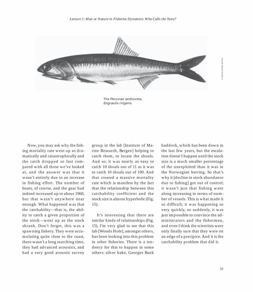
Now, in terms of the Norwegian ment. That’s another of those di- plot), and there is the attempt to re-springs, they are taking a long time agnostics that [shows that] fishing covery along the bottom with the to get back up; just to remind you, has had a very profound effect. You 1973 year class. And it wasn’t until these springs are much more fluc- can’t always get this sort of good the 1983 year class that enabled the tuating than the other ones. They age composition data, but when stock to begin to pick up and then are the ones in Figure 12 with the you can, it adds to the whole inter- it’s the last two, 1990 and 1991, ex-heavy periods of landings from pretation. tremely good year classes, and that 1810 to 1870, a very bad period, stock is back on the map again with and then they came back with a There is the stock-recruitment a replacement line somewhere bang with the 1904 year class diagram (Fig. 14) with the replace- around 0.2 or 0.3. which put it right up and was fol- ment lines going first shallow and lowed by a bigger one. Eventually then up to the top and back again. in the immediate post-war period, The circles show the decline, con-it was at its height with a stock size of 10–12 million metric tons (t) and a very low fishing rate during this period. I’m working on some of their old data now with Ole Johan Østvedt, and it appears that F couldn’t have been much more than about 0.1 during that period. But, then came again some bad year classes and the whole position changed dramatically.
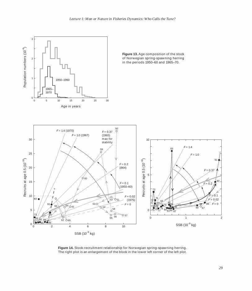
I’ve got a better stock-recruit-ment figure in a moment. What I really want to show in Figure 13 is the age composition in 1965–70 compared to that in 1950–60. This [1950–60] is the period when there were many old fish, right up to 22– 23 years old, with an average age way up in the early teens. By 1965– 70, all of these old fish were gone and we were left simply depending on rapidly declining recruit-
nected with a very difficult-to-draw curve because of the two very good year classes (1950 and 1959), but if you put it somewhere like that, you can see that when they are down here (lower left corner of left plot)—the 1962, 1965, and par-ticularly the 1965, 1967, 1968, 1969 are very poor indeed—the median sort of line, and when it came back from 1973, it was very weak in-deed. You can’t see it from there, so I expanded the square (right
Figure 12. Landings (millions of hectoliters) of winter herring from western Norway. Redrawn from and data through 1960 taken from Devold (1963).
13
12
11
10
9
8
7
6
5
4
3
2
1
Land
ing
s in m
illion
s of h
ectoliters
1760 1770 1780 1790 1800 1810 1820 1830 1840 1850 1860 1870 1880 1890 1900 1910 1920 1930 1940 1950 1960 1970 1980 1990
28
Lecture 1: Man or Nature in Fisheries Dynamics: Who Calls the Tune?
3
Rec
ruit
s at
ag
e 0.
5 (1
0–10 )
Pop
ula
tio
n n
um
ber
s (1
0–9)
1950–1960
1965– 1970
Figure 13. Age composition of the stock 2 of Norwegian spring-spawning herring
in the periods 1950–60 and 1965–70.
1
0 0 5 10 15 20 25 30
Age in years
30
83
73 90
91
85 88
89
50
59
60
53 54
55 56 57
58
52 51
65 62
61 64 66
?
68 69 67
F = 1.4 (1970)
F = 1.0 (1967) F = 0.37 (1965) max for stability
F = 0.2 1964)
F = 0.1 (1950–60)
F = 0.02 (1975)
F = 0
10
25
20
5
15
10
F = 1.4
73
91
90
89
88
83
86 87
F = 1.0
F = 0.37
F = 0.1 F = 0.02
F = 0 67
68 69
70 71
72
74
75
76
77 78
79
8081
8285
F = 0.2
84 5 0
0 1 2
0 0 2 4 6 8 10 SSB (10–9 kg)
SSB (10–9 kg)
Figure 14. Stock-recruitment relationship for Norwegian spring-spawning herring. The right plot is an enlargement of the block in the lower left corner of the left plot.
Rec
ruit
s at
ag
e 0.
5 (1
0–10 )
29

The Raymond J. H. Beverton Lectures at Woods Hole, Massachusetts
Cat
chab
ility
co
effi
cien
t C
atch
abili
ty c
oef
fici
ent
8
0.03
Norwegian spring-spawning herring
b = .0~
A
–1
7
6
5 0.02
4
3
0.01 2
1
0 0 0 10 20 30 40 0 5 10 15
Stock size (no. Z 10–10) Anchoveta biomass (B) (10–6 t)
Peruvian anchovetta; seine
b = 0.97
q = 0.352 x B –0.97
B
0.10
Georges Bank haddock; trawl
r 2 = 0.67
C
b = 0.38
4
0.09
0.08 3
0.07
0.06 2
0.05
0.01
10.03
0.02
0.01 0 0 10 20 30 40 50 60 70 80 0 500 1000 1500 2000 2500
Cape hake; trawl = 1.0
= 10.0
D
VPA b = 0.72
λ
λ
Relative haddock abundance Exploitable biomass (10–3 t)
Figure 15. Plots of catchability coefficient (q) vs. stock size for Norwegian spring-spawning herring (A) (Ulltang, 1980), Peruvian anchoveta (B) (Csirke, 1989), Georges Bank haddock (C) (Crecco and Overholtz, 1990), and Cape hake (D) (Gordoa and Hightower, 1991). Plots were redrawn from figures in these references.
Cat
chab
ility
co
effi
cien
t C
atch
abili
ty c
oef
fici
ent
(10–6
) (m
on
th x
GR
T)
30
Lecture 1: Man or Nature in Fisheries Dynamics: Who Calls the Tune?
© In
stit
uto
del
Mar
del
Per
u
Now, you may ask why the fishing mortality rate went up so dramatically and catastrophically and the catch dropped so fast compared with all those we’ve looked at, and the answer was that it wasn’t entirely due to an increase in fishing effort. The number of boats, of course, and the gear had indeed increased up to about 1960, but that wasn’t anywhere near enough. What happened was that the catchability—that is, the ability to catch a given proportion of the stock—went up as the stock shrank. Don’t forget, this was a spawning fishery. They were accumulating quite close to the coast, there wasn’t a long searching time, they had advanced acoustics, and had a very good acoustic survey
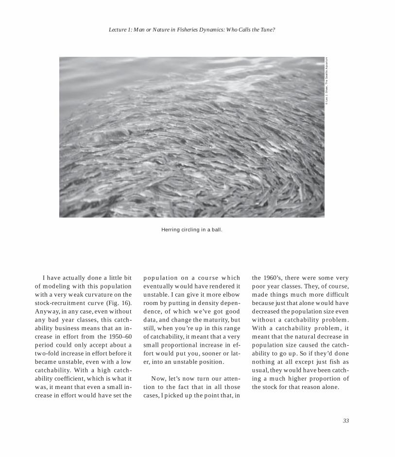
The Peruvian anchoveta, Engraulis ringens.
group in the lab [Institute of Marine Research, Bergen] helping to catch them, to locate the shoals. And so, it was nearly as easy to catch 10 shoals out of 11 as it was to catch 10 shoals out of 100. And that created a massive mortality rate which is manifest by the fact that the relationship between this catchability coefficient and the stock size is almost hyperbolic (Fig. 15).
It’s interesting that there are similar kinds of relationships (Fig. 15). I’m very glad to see that this lab [Woods Hole], amongst others, has been looking into this problem in other fisheries. There is a tendency for this to happen in some others: silver hake, Georges Bank
haddock, which has been down in the last few years, but the escalation doesn’t happen until the stock size is a much smaller percentage of the unexploited than it was in the Norwegian herring. So that’s why it [decline in stock abundance due to fishing] got out of control; it wasn’t just that fishing went along increasing in terms of number of vessels. This is what made it so difficult; it was happening so very quickly, so suddenly, it was just impossible to convince the administrators and the fishermen, and even I think the scientists were only finally sure that they were on an edge of a precipice. And it is the catchability problem that did it.
31

The Raymond J. H. Beverton Lectures at Woods Hole, Massachusetts
LR
DT REF
Unstable
Stable
A
–1.0 –0.5 0
Catchability coefficient
5.0
Unstable
Stable
LRD-D
DT REF
B 5.0
4.0 4.0
3.0 X
incr
ease
in e
ffo
rt
3.0
X X
2.0 2.0
1.0 1.0 –1.0 –0.5 0 –1.0 –0.5 0 +0.1
Xin
crea
se in
eff
ort
Unstable
Stable
12
13
9
6
1
11
10
8
7
5
4
3
2
C
X
Catchability coefficient
Figure 16. Stock-recruitment stability envelopes for Norwegian spring-spawning herring, where X, which is F/(F+M)b, is plotted against catchability for three different assumptions about M (instantaneous natural mortality). F = instantaneous fishing mortality. A: stochastic mode: effect of lognormal recruitment (LR) on reference stability envelope; discrete time (DT) model with zero random recruitment equivalent to reference envelope of steady state model (REF). B: stochastic mode: combined effect of lognormal recruitment and density-dependence of growth and maturity parameters (LRD-D). C: continuation of reference envelope (discrete time model) to positive values of the catchability coefficient.
Catchability coefficient
32
Lecture 1: Man or Nature in Fisheries Dynamics: Who Calls the Tune?
© L
eo J
. Sh
aw, T
he
Sea
ttle
Aq
uar
ium
I have actually done a little bit of modeling with this population with a very weak curvature on the stock-recruitment curve (Fig. 16). Anyway, in any case, even without any bad year classes, this catch-ability business means that an in-crease in effort from the 1950–60 period could only accept about a two-fold increase in effort before it became unstable, even with a low catchability. With a high catch-ability coefficient, which is what it was, it meant that even a small in-crease in effort would have set the
Herring circling in a ball.
population on a course which eventually would have rendered it unstable. I can give it more elbow room by putting in density dependence, of which we’ve got good data, and change the maturity, but still, when you’re up in this range of catchability, it meant that a very small proportional increase in effort would put you, sooner or later, into an unstable position.
Now, let’s now turn our attention to the fact that in all those cases, I picked up the point that, in
the 1960’s, there were some very poor year classes. They, of course, made things much more difficult because just that alone would have decreased the population size even without a catchability problem. With a catchability problem, it meant that the natural decrease in population size caused the catch-ability to go up. So if they’d done nothing at all except just fish as usual, they would have been catching a much higher proportion of the stock for that reason alone.
33

The Raymond J. H. Beverton Lectures at Woods Hole, Massachusetts
Figure 17. Temperature (left) and salinity (right) of the 50–200 m layer in sections A, B, and C, and temperature in 50–200 m in the Kola section (K),
35.2
35.1
35.0
34.9
34.8
B
C
71 72 73 74 75 76 77 78 79 80 81 82 837071 72 73 74 75 76 77 78 79 80 81 82 8370
6
5
4
3
2
1
0
Tem
per
atu
re (
AC)
A
B
K
C
Sal
init
y ( A
A A
A
Year Year )
August–September, 1970–83.
Now, let’s return to the question of what happened in the 1960’s. Well, the answer was that the 1960’s, at least in this part of the North Atlantic, proved to be a very difficult time for fish stocks. The evidence was rather poor, in fact, in the 1960’s; it was nonexistent until quite recently. But, there was a very strong signal coming through in the late 1970’s with temperature and salinity and the polar meridian, which is up off northern Nor-way, showing very distinct dips (Fig. 17), and that’s what started it. What they came up with (Fig. 18) is that this wasn’t just in the late 1970’s, but this was an event that
could be traced back to the mid 1960’s. It was called by Bob Dick-son, Günter Dietrich and others at Kiel, Germany, and Arthur Lee— and there was an ICES Mini-Symposium in the middle 1980’s on it —the “Mid-Seventies Anomaly.” That was a funny name, but it means there were some unusual temperature and salinity events at particular parts of the Norwegian Sea in the North Atlantic. They were able to trace it as a large mass of Arctic water overflowing from the Arctic basin, very cold, much colder than normal. It’s possible, with a certain amount of guess-work, to trace it down on the East
Greenland side, where it got en-trained with the Irminger Current. It circled around off the east coasts of Labrador and Newfoundland and then got tangled up in the early 1970s in the main Gulf Stream and went up much more to the east this time. It looped into the northern North Sea, caused a marked drop in salinity there, and upset the whole Atlantic salmon migration in those 2–3 years, and finally ended up off Norway again, this time much more to the east in the late 1970’s and 1980’s.
So, the extraordinary thing about this is that it took so long to
34

Lecture 1: Man or Nature in Fisheries Dynamics: Who Calls the Tune?
70A
60A
50A
40A
Mid 1960's
1969–70
1971 –72
1973–74
1977 –78
1976– 78
1980–82
1978– 80
50A 40A 30A 20A 10A
Figure 18. Projected track of the “Mid-Seventies” temperature/ salinity anomaly (black) (after Dietrich et al., 1975) and the Gulf Stream (gray).
be picked up. I suppose the answer is, as much as anything, that at-tempting to do any sort of monitoring off the East Greenland coast is extremely difficult. It’s the most inhospitable place to work, with ice traveling at high speeds. I remember trying to get a section done off Cape Farewell, and the innermost
section was 4 miles off. We really much wanted to complete it be-cause we knew we were picking up this very crucial current system. The captain was on the bridge and was watching us like a hawk. He wasn’t watching us as much as he was watching the ice flows moving down on us. Of course, if we’d
had one very close, we’d have had to cut the wire and lose all the water bottles and give it up. Fortunately, we managed to hang on and do it. Trying to do it up off East Greenland would have been much more difficult, and it would have been difficult on the very inhospitable Labrador coast.
35

The Raymond J. H. Beverton Lectures at Woods Hole, Massachusetts
However, there is little doubt 3
that that was what was causing it. 2 In this little diagram I’ve put to-
1gether (Fig. 19), the anomaly of the
no
rmal
zed
fo
r st
ock
siz
e n
orm
alze
d f
or
sto
ck s
ize Norwegian spring-
spawning herring
0
–1
–2
–3 1950 1960 1970 1980 1990
2
1
0
–1
–2
–3
–4
1950 1960 1970 1980 1990
Icelandic spring spawners
2
1
0
–1
–2
–3
Icelandic summer spawners
1950 1960 1970 1980 1990
+1˚
0
–1˚
1950 1960 1970 1980 1990
Year
A
B
D
recruitment success rate, over the long-term average, is taken as a residual in the stock-recruitment curve (Fig. 19A), and shown as a time sequence with the counter-meridian temperatures section, also calculated above and below the means. So I think you can see that without too much difficulty, at least for the Icelandic springs (Fig. 19B) and summers (Fig. 19C), which were much more affected by the anomaly on its way down, as it’s going to the west, fits the lower temperatures. Even though that section (Fig. 19D) isn’t in the right place to catch it, we still see the backwash from it. On the way back, when it was going to the east side, it missed the coastal Icelandic springs altogether, a very weak effect on them. They were far too far to the west, but it really hit the Norwegian spring-spawning her-ring badly in 1979 and 1980. Of course, it was more of a different sort, it wasn’t a temperature signal
Figure 19. Reproductive rate anomalies in the Atlanto-Scandian herring stocks depicted as ∆loge R/S normalized for stock size vs. years (A, B, C) and temperature anomalies at the Kola section (33A30’ E) vs. years (D).
∆lo
ge
R/S
∆
log
e R
/S
no
rmal
zed
fo
r st
ock
siz
ean
om
alie
s (A
C)
Tem
per
atu
re
∆lo
ge
R/S
36
C

Lecture 1: Man or Nature in Fisheries Dynamics: Who Calls the Tune?
5th level
4th level
3rd level
2nd level
1st level
PRODUCERS
C O
N S
U M
E R
S
Sea mammals
Cod
Pred. zoopl.
Juv. gadoids
Capelin Herring Redfish Prawns
Mesozooplankton
Microzooplankton
Macrozooplankton
Phytoplankton
Detritus
Figure 20. Main food webs in the Barents Sea ecosystem (after Ajiad et al., 1992).
here that was doing it, and we’ll come to it in just a moment. So, I think, although this is rather spotty data, and you have to work your way around all the uncertainties, the message is fairly clear. There is a signal coming through here—a message, that is, even despite all the differences of the information.
We now have to answer the question, “Why did Norwegian herring take all through the 1970’s and did not come back up again as the springs did, because the Mid-Seventies Anomaly didn’t affect
them on its way back until the end of the 1970’s.” To do this, we have to go beyond the physical story. We have to look at the whole of the Barents Sea ecosystem (Fig. 20), and I only had time to just pick out a few headlines to remind you it’s what I call an oligospecific system. It’s got a small number of very strongly interacting species, unlike the North Sea or Georges Bank, which has more species and complexities, which certainly Steve Murawski will know because he’s shepherded the Multispecies Working Group through the last 3–4
years. Life in the Barents Sea is a much more straightforward simple system, with much stronger inter-actions on which the main players, leaving aside for the moment—but it won’t last long—the marine mammals, which haven’t been brought in yet, but they’ve got to before long. The Atlantic cod is the main predator, with the capelin and the herring. For the moment, that’s the main triangle that we can look at. They dominate the middle and upper trophic levels. This is a program which the Norwegians and the Russians are doing. There
37
The Raymond J. H. Beverton Lectures at Woods Hole, Massachusetts
Autumn distribution of capelin
Spawning
Franz Josef Land
Novaya Zemlya
Distribution of cod
COD
COD
CAPELIN
Spitsbergen
NORWAY
RUSSIA
of capelin migration
Figure 21. Cod and capelin in the Barents Sea. The winter spawning migration of capelin is shown by the arrows (Tjelmeland, 1992).
have been one or two meetings, but 94] and put in the picture. They’ve they haven’t really started publish- kept me up with what’s going on ing in the full press yet. I’ve had and given me permission to use the privilege of being over in Ber- some of this material in this talk gen in the last year or two [1993– and others.
The interaction, on the other hand, between capelin and cod (Fig. 21) is variable from year to year and greatly complicates the question of measuring the predation effect. But broadly speaking, the capelin moves into the shores to spawn, as it does, of course, in Newfoundland. The cod, to varying degrees, are overlapped in distribution.
Now, I just have to quickly raise the capelin story again (Fig. 22). The stock crashed in the mid-late 1980’s, with a fishing mortality rate again estimating the same problem. The stock-recruitment curve (Fig. 22B) was initially well up, almost throughout this period (1965– 85). In fact, it was capelin that the Norwegian fishing industry went onto when their herring collapsed, and they were managing it very well. There were debates going on between the Norwegian scientists, administrators, and the fishing industry on or about this sort of position until, first in the 1983 year class and then dramatically in 1984, the bottom fell out of the whole thing (Fig. 22A). There were very poor year classes in 1985 and 1986. It’s only been in the last year or two that it’s come back up again.
38

Lecture 1: Man or Nature in Fisheries Dynamics: Who Calls the Tune?
4 2.0
?
C F C
F
A
SSB
Rec
ruit
s at
ag
e 1
(10–1
1 ) C
atch
+ S
SB
(10
–6 t)
3 1.5
2 1.0 F
1 0.5
0 0 1965 1970 1975 1980 1985 1990
Figure 22. Catch (C), spawning stock Year biomass (SSB), fishing mortality rate
(F ), and recruitment in Barents Sea capelin.
12
10
8
6
4
2
0 0 1 2 3 4
B
Cod + herring low
Cod + herring high?
72
73
74
75
76
77
78
79
80
81
82
83
84 85 86 87
88
89
90 91
SSB (10–6 t)
39

The Raymond J. H. Beverton Lectures at Woods Hole, Massachusetts
10
5
0 77 78 79 80 81 82 83 84 85 86 87 88 89 90
Year
Figure 23. Larval index of abundance, spawning stock biomass, and stock biomass at age 2 of Barents Sea capelin (redrawn from Fossum, 1992) compared with cod and herring year-class strength (R ) in numbers.
So, I think now I can show you I’ve just shown you—and that corthe missing jigsaw piece for this responds to the herring and cod (Fig. 23); that is, there are the cape- year classes, of which the 1983 year lin year classes dramatically fall- class (I’ve already mentioned the ing, as measured in the year as 1- herring made a good one), so it was group—so it’s a year less than what for cod. They know from feeding
12
14
10
8
6
4
2
0
1.0
0.8
0.6
0.4
0.2
0
Larv
al in
dex
1981 1982 1983
1984 1985
1986 1987 1988
1989
1990
1991
SS
B (10
–6 t)
Year-class Strength
Cod: R3 (10–8)
Herring: R3 (10–9)
2.0
3.0
4.0
5.0
6.0
? ?
1.0
Stock biomass
(age 2) (10–6 t)
experiments, stomach content analysis, that it (capelin) was essentially very heavily preyed upon by the 1- and 2-group cod, and, to a lesser extent, by herring. The herring story is not so clear, and the cod is very much stronger, and it was this that has caused that particular situation.
Now, the answer so far then is that the cod and herring year classes really hit the capelin hard, but have we explained why the herring didn’t recover until 1983 and why they did then? Well, my theory, which my Norwegian colleagues are treating with some re-serve at the moment, quite understandably, is that what’s happened is that if the herring get re-ally low, which they did in the late 1960’s and early 1970’s, the capelin in effect take over. They are very similar in their ecological status, and it does look very much as if once the herring got below the threshold, caused primarily by fishing, but by a mixture of fishing and the very poor year classes due to the Mid-Seventies Anomaly, the capelin held them down and they couldn’t get back into the system until 1983. And then once that happened, it’s just the whole situation back again, to more like it was when the herring were more abundant. It is, I think, one example as near as I can get to a really good example—there may be several others, but there aren’t many—
40

Lecture 1: Man or Nature in Fisheries Dynamics: Who Calls the Tune?
1.5
1.0
0.5
0
–1.5
–1.0
–1.5
1.5
1.0
0.5
0
–1.5
–1.0
–1.5
77 78 79 80 81 82 83 84 85 86 87 88 89 90 91
1983
0.15
0.10
0.05
0
–0.05
–0.10
–0.15 77 78 79 80 81 82 83 84 85 86 87 88 89 90 91
1983
0.15
0.10
0.05
0
–0.05
–0.10
–0.15
Section A temperature
Section B temperature
Section A salinity
Section B salinity
Sal
init
y (
AAA /
Sal
init
y (
AAA /
∆∆
) )
77 78 79 80 81 82 83 84 85 86 87 88 89 90 91 77 78 79 80 81 82 83 84 85 86 87 88 89 90 91
Year Year
Figure 24. Changes in temperature and salinity conditions at sections A and B off northern Norway, 1977–91.
what ecologists would call alterna- ture and salinity off northern Nor- temperature alone, not because sative stable states. It does look as if, way (Fig. 24) of a kind that hadn’t linity at those ranges is itself necuntil the very good 1983 year class, been seen for some while. Now, essarily harmful, but it could be the herring would have gone on here is the favorable signal [i.e. in more indicative of water condibumping along the bottom, as it 1983]. I don’t know of a mech- tions than temperature alone. But was all through the 1970s. As for anism, and I don’t think anybody whatever it was, that was the phythe question of what caused that does, but I have a feeling, and I sical situation that was associated good year class, the best clue is that shall mention it again in the last with the timing with those two in 1983 there was a very consider- part of my talk, that the salinity sig- good year classes in both species. able upward blip in both tempera- nal is a better diagnostic than the
∆Te
mp
erat
ure
(AC
) ∆
Tem
per
atu
e (A
C)
41
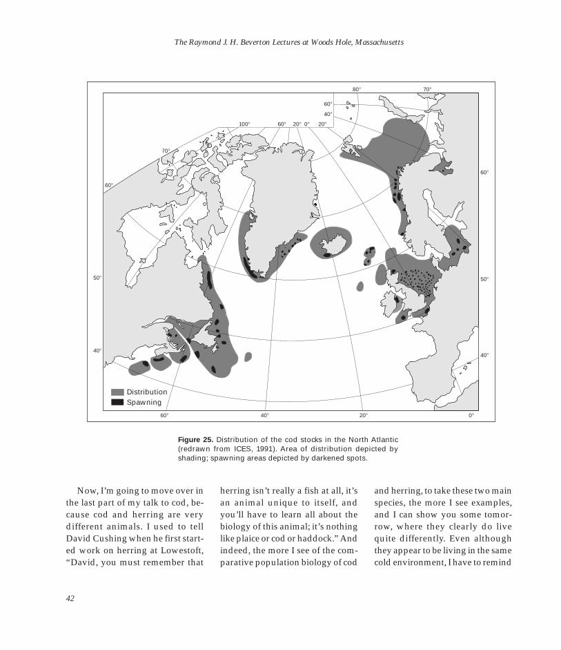
The Raymond J. H. Beverton Lectures at Woods Hole, Massachusetts
Distribution Spawning
60A
70A
100A 60A 20A 0A
80A 70A
50A
40A 40A
50A
60A
20A
40A
60A
60A 40A 20A 0A
Figure 25. Distribution of the cod stocks in the North Atlantic (redrawn from ICES, 1991). Area of distribution depicted by shading; spawning areas depicted by darkened spots.
Now, I’m going to move over in the last part of my talk to cod, be-cause cod and herring are very different animals. I used to tell David Cushing when he first started work on herring at Lowestoft, “David, you must remember that
herring isn’t really a fish at all, it’s an animal unique to itself, and you’ll have to learn all about the biology of this animal; it’s nothing like plaice or cod or haddock.” And indeed, the more I see of the comparative population biology of cod
and herring, to take these two main species, the more I see examples, and I can show you some tomorrow, where they clearly do live quite differently. Even although they appear to be living in the same cold environment, I have to remind
42

Lecture 1: Man or Nature in Fisheries Dynamics: Who Calls the Tune?
57A
60A
63A
66A
69A
80A 76A 72A 68A 64A 60A 56A 52A 48A 44A 40A 36A 32A 28A 24A 20A 16A 12A
72A
69A
63A
60A
57A
28A32A36A40AW44A48A52A56A60A
66A
Subarctic water
West Greenland Current
100 0 500 km
Greenland
Iceland
Polar Current (cold)
Irminger Current (warm)
Spawning grounds of West Greenland cod
Spawning grounds of Icelandic cod
Figure 26. Surface currents (redrawn from Hansen and Hermann, 1953) and cod spawning grounds in Greenland waters.
you that we are talking about a whole series of cod populations scattered over the northern fringe (Fig. 25), a fascinating distribution because it gives you a double-degree temperature gradient each side of the Atlantic, with some very
fringe physical conditions, around Greenland, in the middle. I expect you know the Greenland story pretty well (Fig. 26). There is the current system, the warm [Irminger Current], the cold [Polar Cur-rent] coming around West Green-
land. The spawning area, when there are fish to spawn, is off the West Greenland side. The story is one of these where there’s no question of disentangling the effects here, not the start of it anyway or indeed the finish of it. There are
43
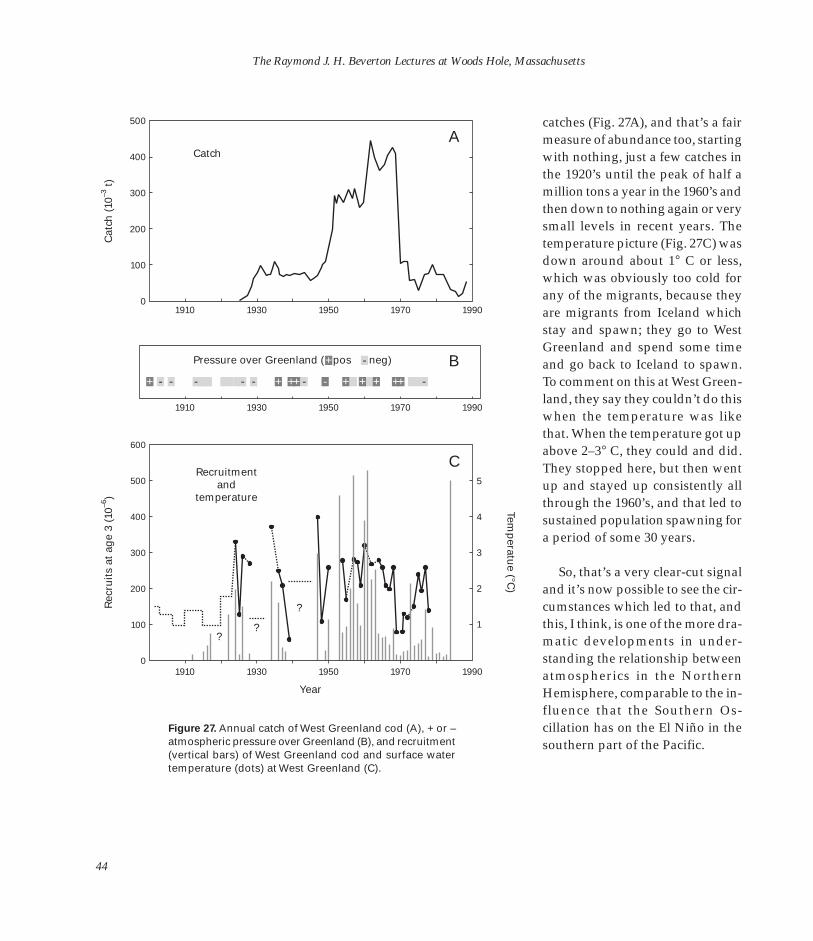
- - - - - - - - -
The Raymond J. H. Beverton Lectures at Woods Hole, Massachusetts
Rec
ruit
s at
ag
e 3
(10–6
) C
atch
(10
–3 t)
500
400
300
200
100
0 1910 1930 1950 1970 1990
Catch A
1910 1930 1950 1970 1990
600
500
? ?
?
Recruitment and
temperature
C 5
400 4
300 3
200 2
100 1
0 1910 1930 1950 1970 1990
Year
Figure 27. Annual catch of West Greenland cod (A), + or – atmospheric pressure over Greenland (B), and recruitment (vertical bars) of West Greenland cod and surface water temperature (dots) at West Greenland (C).
Temp
eratue (AC
)
catches (Fig. 27A), and that’s a fair measure of abundance too, starting with nothing, just a few catches in the 1920’s until the peak of half a million tons a year in the 1960’s and then down to nothing again or very small levels in recent years. The temperature picture (Fig. 27C) was down around about 1A C or less, which was obviously too cold for any of the migrants, because they are migrants from Iceland which stay and spawn; they go to West Greenland and spend some time and go back to Iceland to spawn. To comment on this at West Green-land, they say they couldn’t do this when the temperature was like that. When the temperature got up above 2–3A C, they could and did. They stopped here, but then went up and stayed up consistently all through the 1960’s, and that led to sustained population spawning for a period of some 30 years.
So, that’s a very clear-cut signal and it’s now possible to see the circumstances which led to that, and this, I think, is one of the more dramatic developments in under-standing the relationship between atmospherics in the Northern Hemisphere, comparable to the influence that the Southern Oscillation has on the El Niño in the southern part of the Pacific.
Pressure over Greenland ( pos neg)
+ - - - - - - - -+ ++ + + + ++
+ - B
44
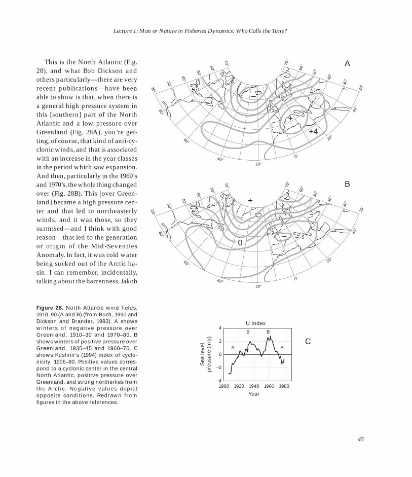
Lecture 1: Man or Nature in Fisheries Dynamics: Who Calls the Tune?
This is the North Atlantic (Fig. 28), and what Bob Dickson and others particularly—there are very recent publications—have been able to show is that, when there is a general high pressure system in this [southern] part of the North Atlantic and a low pressure over Greenland (Fig. 28A), you’re getting, of course, that kind of anti-cyclonic winds, and that is associated with an increase in the year classes in the period which saw expansion. And then, particularly in the 1960’s and 1970’s, the whole thing changed over (Fig. 28B). This [over Green-land] became a high pressure center and that led to northeasterly winds, and it was those, so they surmised—and I think with good reason—that led to the generation or origin of the Mid-Seventies Anomaly. In fact, it was cold water being sucked out of the Arctic basin. I can remember, incidentally, talking about the barrenness. Jakob
Figure 28. North Atlantic wind fields, 1910–90 (A and B) (from Buch, 1990 and Dickson and Brander, 1993). A shows
70A60A50A40A30A20A
70A
60A
50A
40A
30A
20A
80A
60A
40A 20A
0A
20A
40A
70A60A50A40A30A20A
70A
60A
50A
40A
30A
20A
80A
60A
40A 20A
0A
20A
40A
A
B
+4
0
+
+
–
–
winters of negative pressure over Greenland, 1910–30 and 1970–80. B shows winters of positive pressure over Greenland, 1935–45 and 1960–70. C shows Kushnir’s (1994) index of cyclonicity, 1906–80. Positive values correspond to a cyclonic center in the central North Atlantic, positive pressure over Greenland, and strong northerlies from the Arctic. Negative values depict opposite conditions. Redrawn from figures in the above references.
Sea
leve
l p
ress
ure
(m
b)
U index 4
2
B
A
B
A C
0
–2
–4 1900 1920 1940 1960 1980
Year
45

The Raymond J. H. Beverton Lectures at Woods Hole, Massachusetts
NE Arctic cod
W Greenland cod
P R 2
<0.01
<0.001
7
67 8
7
6
5
4
3
2 0 0.5 1.0 1.5 2.0 2.5 3.0 3.5 4.0
Temperature (AC)
Figure 29. Year-class strength vs. temperature on the spawning grounds for Northeast Arctic and West Greenland cod.
–6)
Log
e re
cru
its
at a
ge
3 (1
0
Jakobsson recalls how he was off northern Iceland at this time in the middle 1960’s and he said that the sea was just crystal clear, very cold, and actually devoid of any obvious life. I can remember trawling—we had some time on our hands and it was very good weather—in the late
1950’s. We trawled right around the top of Spitsbergen doing a bit of fishing as we went. We got broken up a lot, lots of rocks up there, but we hardly caught a thing. The net would come up after 3 hours with virtually nothing in it. It was clear, very clear, very cold, and
very fresh. So, that sort of Arctic water—I don’t know if it’s true of the Arctic basin generally, but that could possibly have been Arctic water coming down—was clearly very inhospitable to anything from primary production onwards. I think that is rather a very convin-
46
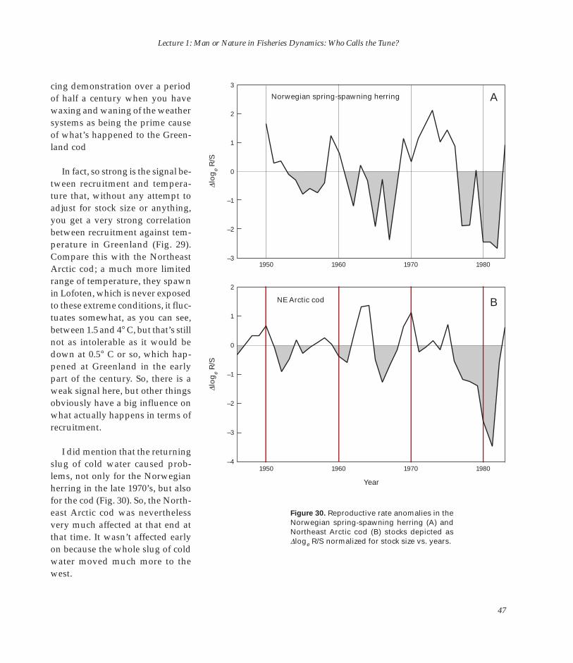
Lecture 1: Man or Nature in Fisheries Dynamics: Who Calls the Tune?
cing demonstration over a period of half a century when you have waxing and waning of the weather systems as being the prime cause of what’s happened to the Green-land cod
In fact, so strong is the signal be-tween recruitment and temperature that, without any attempt to adjust for stock size or anything, you get a very strong correlation between recruitment against temperature in Greenland (Fig. 29). Compare this with the Northeast Arctic cod; a much more limited range of temperature, they spawn in Lofoten, which is never exposed to these extreme conditions, it fluctuates somewhat, as you can see, between 1.5 and 4A C, but that’s still not as intolerable as it would be down at 0.5A C or so, which happened at Greenland in the early part of the century. So, there is a weak signal here, but other things obviously have a big influence on what actually happens in terms of recruitment.
I did mention that the returning slug of cold water caused problems, not only for the Norwegian herring in the late 1970’s, but also for the cod (Fig. 30). So, the North-east Arctic cod was nevertheless very much affected at that end at that time. It wasn’t affected early on because the whole slug of cold water moved much more to the west.
∆lo
ge
R/S
∆
log
e R
/S
3
2
1
0
–1
–2
–3
2
1
0
–1
–2
–3
–4 1950 1960 1970 1980
1950 1960 1970 1980
Norwegian spring-spawning herring
NE Arctic cod B
A
Year
Figure 30. Reproductive rate anomalies in the Norwegian spring-spawning herring (A) and Northeast Arctic cod (B) stocks depicted as ∆loge R/S normalized for stock size vs. years.
47

The Raymond J. H. Beverton Lectures at Woods Hole, Massachusetts
–9)
Cat
ch a
nd
SS
B (
10–6
)R
ecru
its
at a
ge
3 (1
0
3
SSB
F
A
C
1.5
2.5
2 1.0
1.5 F
1 0.5
0.5
0 0 1950 1960 1970 1980 1990
Year
2
1
0 0 0.5 1.0 1.5
F = 0
F0.1 = 0.14
F max = 0.25
Fmed = 0.46
F = 0.33
F = 0.58 50
51
52
53
54
55
56
57 58
59
60
61
62
63
64
65
66 67
68
69
70
91
71
72 73
74
75
76 77
78 79 80
81
82
83
84 85
86
88
89
90
B
87
SSB (10–6 t)
Figure 31. Catch (C), spawning stock biomass (SSB), fishing mortality rate (F ), and recruitment in Northeast Arctic cod.
Just to see what the picture looks like for cod, there is the general story (Fig. 31), nothing like the dramatic collapse that we see in the pelagics, but a steady attrition on its stock size over a long period, except at the very end when two very good year classes would come in (Fig. 31A). The fishing mortality rate was gradually increasing up to a pretty high level, nearly 1, which is nothing like the extremes of the Norwegian spring-spawning her-ring fishery, but it’s still pretty high. In terms of a stock-recruitment diagram (Fig. 31B), we haven’t got, of course, the collapse and recovery in the same sort of way. The nearest you can get to it is the upper arrowed line, with the replacement lines, unexploited at one point, steepening, as they did, right up to another point, leaving still a possibility of a stable sustainable situation, a very poor one in terms of stock size and yield, but nevertheless sustainable when recruitment was between 0.4 and 0.5 x 10⁹ and SSB was between 0.2 and 0.4 x 10⁶
t. But you see again there were some very poor year classes, and these have helped pull the thing down.
The other important cod fishery, the Icelandic (Fig. 32), has a rather similar story: slow decline, a bit steeper, the stock size is a bit more erratic, and a gradual climb in fishing mortality nearly the same amount. There is a more strongly
48
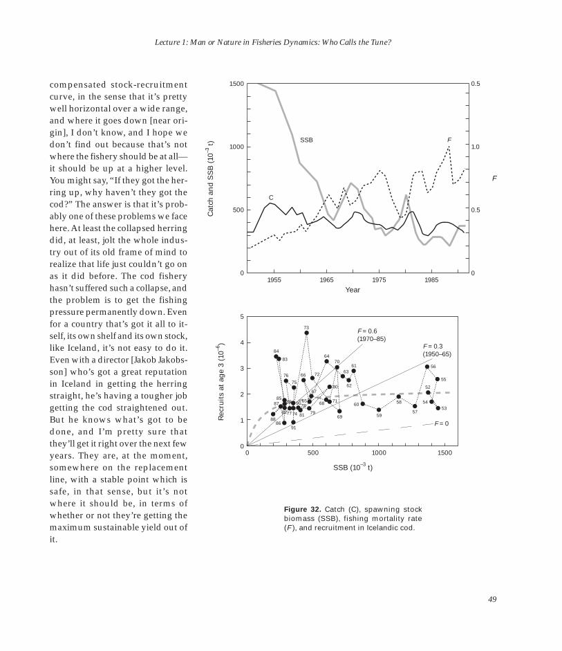
Lecture 1: Man or Nature in Fisheries Dynamics: Who Calls the Tune?
compensated stock-recruitment curve, in the sense that it’s pretty well horizontal over a wide range, and where it goes down [near origin], I don’t know, and I hope we don’t find out because that’s not where the fishery should be at all— it should be up at a higher level. You might say, “If they got the her-ring up, why haven’t they got the cod?” The answer is that it’s probably one of these problems we face here. At least the collapsed herring did, at least, jolt the whole industry out of its old frame of mind to realize that life just couldn’t go on as it did before. The cod fishery hasn’t suffered such a collapse, and the problem is to get the fishing pressure permanently down. Even for a country that’s got it all to it-self, its own shelf and its own stock, like Iceland, it’s not easy to do it. Even with a director [Jakob Jakobsson] who’s got a great reputation in Iceland in getting the herring straight, he’s having a tougher job getting the cod straightened out. But he knows what’s got to be done, and I’m pretty sure that they’ll get it right over the next few years. They are, at the moment, somewhere on the replacement line, with a stable point which is safe, in that sense, but it’s not where it should be, in terms of whether or not they’re getting the maximum sustainable yield out of it.
–3 t)
Cat
ch a
nd
SS
B (
10
1500
C
SSB F
0.5
1000 1.0
F
500 0.5
0 0 1955 1965 1975 1985
Year
5
4
3
2
1
0 0 500 1000 1500
F = 0.6 (1970–85)
F = 0.3 (1950–65)
F = 0
52
53 54
55
56
57
58
59
60
61
62
63
64
65
66
67
68
69
70
71
72
73
74
75
76
77
78
79
80
81 82
83
84
85
86
87
88
89 90
91
SSB (10–3 t)
Figure 32. Catch (C), spawning stock biomass (SSB), fishing mortality rate (F ), and recruitment in Icelandic cod.
–6)
Rec
ruit
s at
ag
e 3
(10
49

The Raymond J. H. Beverton Lectures at Woods Hole, Massachusetts
Now, it would be, I think, inappropriate to finish my lecture with-out some mention of the northern cod, much closer at hand on the western side. May I say straight away that I don’t think it’s very wise for an outside person to try and tell the professionals on the spot what their answer is or what their job should be, in the sense of sorting this out. It’s problem enough, a desperate problem, with having an industry virtually crippled like this. But it did seem to me that if I am going to try to give you this kind of scan around what’s happened to some of these fish stocks, in terms of the interplay be-tween fishing and natural causes, it would be inappropriate not to mention this one because it’s, in some ways, the most unexpected and the most dramatic of all. At least the herring stocks that we’ve looked at, many of them, those that we know a long history of, there’s been a history of instability. So it’s not all that surprising if we’re in the middle of one now. But I think your northern cod have never had anything near that degree of erratic behavior in the past, at least not that I’m aware of. The Grand Banks fisheries have been going more or less off and on with some fluctuations, but they’ve going for many hundreds of years.
Now, this seemed to me to be a critical diagram (Fig. 33). This is in Rivard and Maguire (1993) from
Yie
ld (
t)
900,000
800,000
700,000
600,000
500,000
400,000
300,000
200,000
100,000
0 0 0.1 0.2 0.3 0.4 0.5 0.6 0.7 0.8 0.9 1 1.1 1.2
1962
1990 1976
Equilibrium yield in the early 1970's
Equilibrium yield in the late 1980's
F
Figure 33. Productivity of the northern cod stock (NAFO Div. 2J3KL). The productivity of the early 1970’s is compared with that of the late 1980’s.The productivity curves correspond to the yield per recruit (using the growth characteristics for these periods and assuming knife-edge selection at age 5) multiplied by the average recruitment for the year classes contributing to these periods (redrawn from Rivard and Maguire, 1993).
the Canadian workshop on Risk Evaluation and Biological Reference Points for Fisheries Management which was held a few years ago. They plotted the actual yield against fishing mortality rate
in the 2J3KL and 3NO stocks, the Labrador and northern banks stocks. They regard this as a quasi stable point there [about 450,000 t], and another one here [about 200,000 t], but the yield’s half that,
50
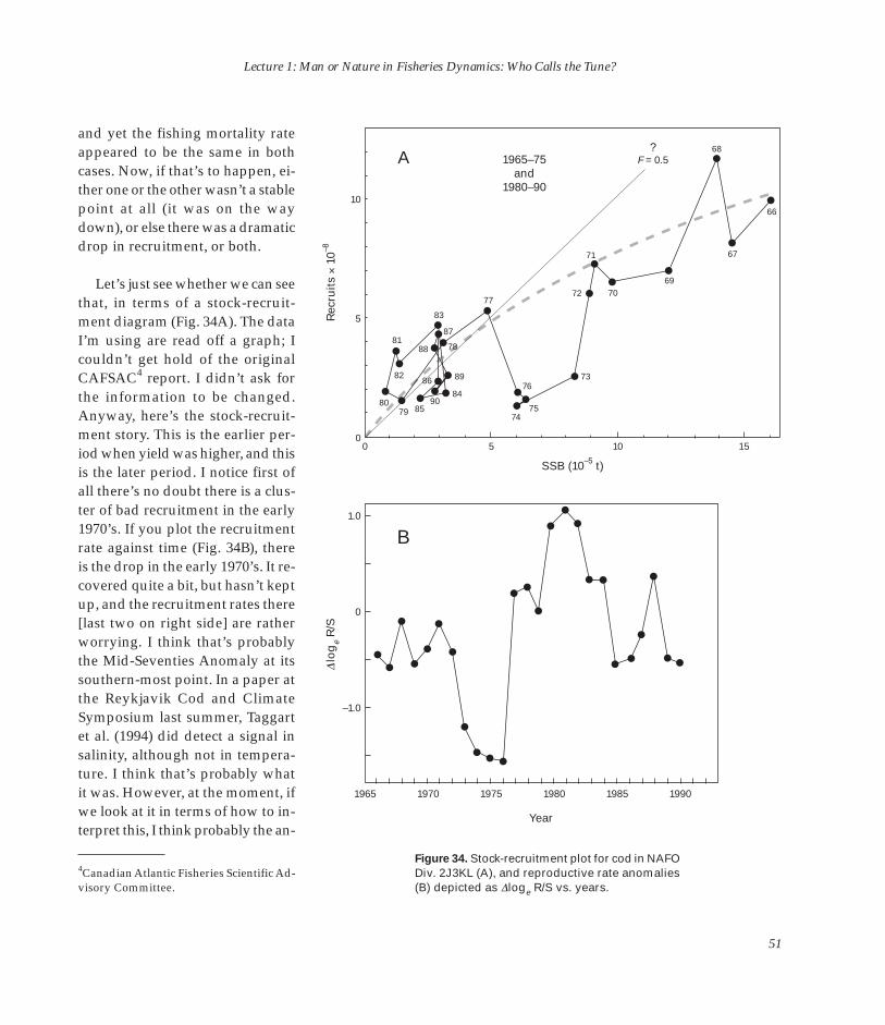
Lecture 1: Man or Nature in Fisheries Dynamics: Who Calls the Tune?
and yet the fishing mortality rate appeared to be the same in both cases. Now, if that’s to happen, either one or the other wasn’t a stable point at all (it was on the way down), or else there was a dramatic drop in recruitment, or both.
Let’s just see whether we can see that, in terms of a stock-recruitment diagram (Fig. 34A). The data I’m using are read off a graph; I couldn’t get hold of the original CAFSAC4 report. I didn’t ask for the information to be changed. Anyway, here’s the stock-recruitment story. This is the earlier period when yield was higher, and this is the later period. I notice first of all there’s no doubt there is a cluster of bad recruitment in the early 1970’s. If you plot the recruitment rate against time (Fig. 34B), there is the drop in the early 1970’s. It re-covered quite a bit, but hasn’t kept up, and the recruitment rates there [last two on right side] are rather worrying. I think that’s probably the Mid-Seventies Anomaly at its southern-most point. In a paper at the Reykjavik Cod and Climate Symposium last summer, Taggart et al. (1994) did detect a signal in salinity, although not in temperature. I think that’s probably what it was. However, at the moment, if we look at it in terms of how to interpret this, I think probably the an-
4Canadian Atlantic Fisheries Scientific Advisory Committee.
∆lo
ge
R/S
R
ecru
its
Z 10
–8
1965–75 and
1980–90
? F = 0.5
67
66
68
69 70
71
72
73
74 75
76
77
78
79 80
81
82
83
84
85
86
88
87
89
90
A
10
5
0 0 5 10 15
SSB (10–5 t)
1.0
0
–1.0
B
1965 1970 1975 1980 1985 1990
Year
Figure 34. Stock-recruitment plot for cod in NAFO Div. 2J3KL (A), and reproductive rate anomalies (B) depicted as ∆loge R/S vs. years.
51

The Raymond J. H. Beverton Lectures at Woods Hole, Massachusetts
swer is it wasn’t in equilibrium, it wasn’t a stable point here. If you had a safe fishing rate then, you must have more or less the same replacement line, subject to growth rates and things not being all that dissimilar. If it’s stable down here [lower left side of Fig. 34A], which is where it might just be or where it was in the 1980’s, it could not be up there [on the F = 0.5 replacement line], and I think the reason for this is that it’s a very shallow curve. This is a very weakly compensated stock on the northern end of its limits, which is what we would expect. Alec MacCall’s ideas on dynamic geography of fish stocks would suggest exactly that. Stocks at the fringe of their distribution have a very weak density dependence, but are very much influenced by the environment, a harsh environment. And we can probably see, rather like the Norwegian herring story, a very potentially unstable population doesn’t take a lot of fishing to drive it down. Fishing at that level is almost certainly too much for it, but that isn’t, of course, the real answer. I think the real answer to the immediate problems must lie in this very massive downward push of cold water. It’s almost like a cold slug coming down (the Mid-Seventies Anomaly) the Labrador coast and pushing everything in its path.
There are still some unexplained events. Why the fish have gone into deeper water may be to get away from the temperature. Whether the capelin is partly responsible, I think it’ll be a little while yet be-fore we really know the answer. But it is one of the most disturbing of all the events I’ve seen and heard in my time because it really seems to be unexpected. But it’s so wide-spread and so dramatic, and fishing may have weakened the stock, in the sense that it was, the north-ern one in particular, a very poorly compensated one, but it wasn’t an escalation problem like as the her-ring had been, I’m sure.
So, let’s see if I can sum up now, for I’ve been talking longer than I should have anyway. I think the picture that I get from all this is how complex the environment is in time and space. It is only when things really become very sharply defined, as in the extremes of marginal habitats or in extremely escalating fishing pressures, that we really become convinced of what’s happened without having to weigh one thing up too carefully with an-other.
In terms of the small pelagics that we were looking at—the top ten—there was only one that really disappeared and never came back. That was the Icelandic springs, but two or three others that were clearly on the way down—and
what fishing did was to hasten them on their way and push them over the edge—would have gone anyway in time. Then there would be the intermediate case where they would have been in a pretty poor state, but they were driven down by fishing in such a way that when there was some adverse environmental condition, you were in a pretty poor state to deal with it. There’s no doubt fishing pushed down the Norwegians particularly, and southern North Sea herring as well, and several of the others, into a state much lower—much, much lower—than they would have been in just on their own, and indeed this happened in the case of the Norwegian one—it upset the whole balance of the ecosystem in the process. Finally, for those for which the Icelandic summer spawners is a good example, where they are pretty resilient and fishing did push them down quite a bit, no doubt about it, they probably would have just done a little blip and ridden out one or two bad year classes quite easily, but having been pushed down, they at least came back up again quite quickly.
So, can we make any sort of check list of [situations] when fishing is a real threat, in the light of this review (Fig. 35). I still think that the most important single thing, as far as the fishing side, is when catchability escalates out of control, and especially when a de-
52

Lecture 1: Man or Nature in Fisheries Dynamics: Who Calls the Tune?
Fishing poses a threat to sustainable harvesting and, potentially, to the viability of the resource, when:
1. Catchability escalates out of control, especially when accentuated by a declining stock whose reproductive potential has been weakened by adverse environmental conditions.
2. Long-term fishing capacity is maintained or increased by political/economic incentives remote from, ignorant of, or indifferent to the long-term productivity of the resource.
3. The species is caught incidentally, but is more vulnerable than the target species.
4. Capture is by interception on a migration route to a spawning ground, making it possible to harvest the whole spawning stock with no immediate economic penalty.
5. These threats are compounded if the species is: a) long-lived, b) has a low per capita reproductive rate, c) has a weakly compensated parent-progeny relationship, d) is easily accessible and cheap to catch, and e) has a high market value.
In these circumstances, clear objectives, good science, strong political will, firm control, and a cooperative fishing community are more than usually necessary for sustainable harvesting and good resource husbandry.
clining stock’s reproductive potential has been weakened by adverse environmental conditions, which was true for some of the herring examples. That’s a very serious situation. Another one is when the long-term fishing capacity is maintained or increased by political and economic incentives remote from, ignorant of, or indifferent to the
Figure 35. Summary points.
long-term productivity of the re-source. Now that’s a rather pompous sort of statement, but what I’m trying to say is that this is where management in general, or industry or whatever, just doesn’t see what is happening, and maybe until there is rapid escalation of fishing, it’s hard to expect that they could. There are many other cases
where they could see it, and you have some on your doorstep and I don’t need to remind you of them.
When a species is caught incidentally, of course, but is more vulnerable than the target species, that creates a problem we haven’t talked about, but it is obviously a problem. There are some examples,
53
The Raymond J. H. Beverton Lectures at Woods Hole, Massachusetts
possibly one of the rays, the common skate in the Irish Sea, that seems to have disappeared, probably because it was caught not as a target species, but was taken very easily while fishing for other species. This is a general category, and it is not just on marine species either. Another is when you’re intercepting fish on the migration route, more especially in rivers, and you can take the whole run totally with-out any immediate economic penalty for so doing. You just wake up to the fact the next day there aren’t any fish left. That is an extreme case, but there are some other examples in the marine fisheries where it gets quite close to that sort of thing.
Problems in all those situations can be compounded: the species is long-lived, it has a low per-capita reproductive rate anyway. In other words, it has a low fecundity rate and a low birth rate, so it’s not able to ride out these troubles. It has a weakly compensated parent-progeny relationship, such as some of those I’ve shown you. Of course, it is easily accessible, cheap to catch, and has a high market value, which adds to the problem. Under these circumstances, fair objectives, good science, strong political will, and firm control by a cooperative fishing community are more than usually necessary for sustainable harvesting and good husbandry. Usually one will say, “Yes, that’s what
we’re doing; we’re very familiar with that situation.”
Well, I started to ask the question right at the beginning: “Who calls the tune?” Perhaps if I just simply finish by saying that it seems to me nature decides what the melody should be and produces the score, and man has to decide how he going to play it. It might be a very complex score, and it might be that an orchestra is needed to play. Therefore, it depends very much on whether the conductor can read the score in the first place, and whether his musicians can play their instruments decently. I’m afraid the record shows that most of the time man makes a right old hash of playing most of the scores that nature produces. The only possible excuse is that nature will produce a new score at the last minute. The concert will be halfway through, and along will come the second half of the concerto which will require a new score that nature’s just produced. But we haven’t seen that one before, so we’ve got to be good at sight reading and we’ve got to have a good memory, and we’re not good at either of those things. Thank you very much.
Emory Anderson Ray has talked for a little over
an hour, but I’m sure he’d be willing to answer a few questions at least. Do any of you have particu
lar comments? I see a few hands going up.
Andy Rosenberg I wonder if maybe you have a
unique perspective because you watched the development of a lot of these fisheries, both as they were going up and when they came down again. Some of us, I guess, only saw them coming down. Do you think it’s possible, given those pictures of stock and recruitment that you have, to have been able to diagnose what was going on at the time? In other words, to use your musical analogy, instead of knowing or having rehearsed the score in advance, could you have predicted what was going to happen?
Ray Beverton I don’t think, at the time (the
1950’s), that we had the experience, the know-how, or the evidence to really pick up anything like the pulse. So I don’t really think there was much that could have been done at the time. But another aspect of your question is whether we could again pick it up, armed with what we now know. I think this is a very important question. One thing that could be done, and I’ve thought about trying to do it, but I haven’t got around to it yet, and it may be something which needs more advanced computing than I can do now, is to actually try to hindcast backwards.
54

Lecture 1: Man or Nature in Fisheries Dynamics: Who Calls the Tune?
Supposing we really were on that and we didn’t have those two year classes or supposing we had stopped fishing when the stock, such as the Norwegian herring, had fallen to, say, 4 million t, could they have held it at that point, could it have sustained itself with no fishing then, not waiting until they had no fish and then stop fishing? That means you’ve got to be able to predict, given the recruitment rate at that moment from your expected curve and the actual thing, whether you could safely assume that’s what would have happened if you’d had a bigger stock. The trouble with the herring is you would have a great problem, if I’m right, because of the threshold beyond which capelin takes over. But you could hindcast the Icelandic one, the summer spawners, I think. Reversibility enables a hindcasting to be done.
Say, had you stopped at such and such a point, this is what would have happened. And I think this sort of approach—I’ll call it sophisticated hindcasting—is some-thing we really ought to develop. I think it’s maybe possible, especially with computer interaction. Fishermen are prepared to listen and are able to respond, and you can say to them, “Look, here’s what actually happened, remember? Now, this is the story of what we’ve done. Now try and press this but-ton and see what would happen if
you had done that.” In Australia, they actually did something like this for one of their little inshore fisheries. I believe it’s something we should do. How you put it across is another thing. Only those who know their fishermen and know how to talk to them should say how to do it, but it seems to me we have an opportunity here, with data as good as that, for some of us to hindcast and say, had we been able to hold the fishing back, keep the fishing mortality down, we could predict with some reasonable precision what would hap-pen. I don’t think we’d really start doing it very systematically, but I think it would be very valuable to do. I don’t know if that is what you had in mind, Andy, but it’s certainly what your question triggered off in my mind.
Andy Rosenberg Yes, I think it is what I had in
mind. Even if you took on some of these stock-recruitment plots and blocked out the information so you just looked at the first 10 years to see what you would come to, and then 20 years, and so on. If you could actually come to a conclusion, that would reasonably suggest what would happen next. Now, that’s difficult to do because, of course, you have only one his-tory to pick.
Ray Beverton I think in some of our stock-re
cruitment data—and they look awful on the diagram—there really is a lot more information. There is an enormous amount of information in them, and if it is possible to manipulate them in such a way, you could draw out a signal from a mass which, at first sight, seems to be impossible.
George Kelly If a bumper year class of any of
the major species in the North Atlantic were to come, is anyone pre-pared to manage them scientifically or otherwise?
Ray Beverton Well, I gave you the example of
the summer-spawning herring which the Icelanders are doing, exactly on that basis.
George Kelly Is it the Norwegians who were
responsible?
Ray Beverton No, this is the Icelanders. It was
not an ICES fishery because once Iceland had extended her 200-mile limit, this put both their herring and their cod entirely under their own jurisdiction. So it never came to either NEAFC5 or the EC6 be-cause it was outside the jurisdiction of both. And indeed, it wasn’t until about 3 or 4 years ago that the
5North-East Atlantic Fisheries Commission. 6European Commission.
55

The Raymond J. H. Beverton Lectures at Woods Hole, Massachusetts
story has really been produced at ICES scientifically. I think I can take a very modest credit for persuading Jakob: “Now come on Jakob, you’ve got a wonderful story here, you must put this into the ICES bowl.” He did it; he and Gunnar Stefánsson, his very good statistician, have done this very effectively. So, they’re doing it, but the Norwegians are doing it with the Russians now. The Russians, of course, are very much affected by the recent upheaval in Russia. That’s what’s led to the withdrawal of much of the Russian fishing pressure and enabled the fishing mortality rate to dramatically drop up in the north, on the Arctic cod in particular. That one I’m hoping they will be managing in accordance with this joint Russian-Norwegian multispecies exercise they’re getting now. They’ve got to make a decision as to how much more cod they want. If they really bring the cod anywhere near to its maximum, they’re not going to have anything like the capelin fishery they’ve got. And the herring is, at the moment, the joker in the pack. They haven’t really got that put into the system, but they’ve got a decision to make about how to balance between these three major species.
George Kelly Did you say you were optimis
tic for the future of the fisheries in the north?
Ray Beverton For that one I am, as long as the
Russians can keep up with it, as it were, and put into practice what their scientists are saying. Their scientists are pretty involved in this, but it’s a question of whether they can deliver the goods. But I think there is a good chance for that, and I think we’ll see the Ice-land cod coming under a better management before long. As to the rest of it, that’s a different matter, at least on our side of the Atlantic it’s a very different problem and something I might talk about to-morrow, but that’s another story.
George Kelly You mentioned the California
sardine only in passing, but I didn’t get whether you were attributing [the problems to] man’s operation or the environment.
Ray Beverton Both were to blame, I’m pretty
sure. You have an upwelling that was causing periodic upheavals, and every time there was a bit of a drop in the stock size, up would go the catchability. So the effort was suddenly taking a lot more [fish] than it should have been. And then there was another bit of a relaxation [in effort]. It dribbled around in a half-baked state between sort of going off and finally it did tip over and went down, with, of course, the sardine coming back up again, I mean in that case the Pa
cific sardine. That’s happened in historical times, so we’ve seen the alternation between sardine and northern anchovy, I mean in this case, and so also in the Peruvian story. There’s some very complicated, knock-on effects once either man or nature starts really to up-set the system to this extent.
Steve Murawski In the last few years, the concept
of sustainability has entered into a lot of our natural resource management, at least in theory if not in practice. I wonder, given the interplay between environment and fishing mortality, if sustainability as a concept in fisheries is really an unattainable goal?
Ray Beverton I very firmly believe that it is a
perfectly attainable goal, provided we can really get the fishing pressure down to where we often said it should be, which is down well below F max. Then you are to a point at which none of the stock-recruitment arrays I’ve seen, the replacement line, would be anywhere near a nonsustainable situation. So I think any stock that cannot sustain a doubling of its natural mortality rate would be in difficulty anyway, because that could easily happen for natural reasons. I’m trying to put some evidence together on this one. I don’t think there will be time tomorrow, but I think I can begin to show that you’ve got, histori-
56

Lecture 1: Man or Nature in Fisheries Dynamics: Who Calls the Tune?
cally, some pretty sustainable situations provided you can get that fishing mortality right down. It’s not a new thing; if you like, it’s Gulland’s F0.1 (Gulland and Boerema, 1973). I would not put it in terms of economics. I’d just say, for goodness sake, get that fishing pressure down to something around about the natural mortality rate or not much more. You may say that’s not proof that it’s sustainable, but you have then to rely upon all the background evidence that you’ve got about what’s made things unsustainable and make sure you’re not in that situation. You could, at least in the negative sense, say that we’ll avoid all those situations that in the past made it unsustainable. Not a particularly convincing answer, but you asked me a very pro-found question which I think is a vitally important one which we’ve got to face in terms of the Rio Con-vention7 and all those sorts of things—sustainability and biodiversity. But a fishing pressure of an amount that is not more than, at the most, twice the natural mortality rate and preferably less, is below Fmax usually, and that means only a biomass of about half the unexploited biomass or at most one-third of it.
7United Nations Conference on Environment and Development (UNCED) held in Rio de Janeiro, Brazil, in June 1972.
Steve Murawski I think it’s safe to say we can find
fishing mortality rates that are so low that would guard against almost any sort of fluctuation in the environment. On the other hand, that may be the price of a tremendous foregone yield in times when, in fact, there are good year classes to harvest.
Ray Beverton If you approach it in terms of
keeping a harvesting rate at a very modest level, you will then have to accept that, if you’ve got some good year classes, you will get better yields, but the harvesting rate will still be the same. Now, that’s not what the industry likes; they want stability. I think the industry’s pressure for stability has been one of the real difficulties that has caused us to try to manage stability by fiddling about with the harvesting rate. John Shepherd tried at an ICES Dialogue Meeting (ICES, 1990) to convince our industry that you can’t have both good husbandry and try and stabilize it all by fiddling about with the harvesting rate. Fishermen know in the past that their resources have fluctuations; they expect good years and bad years. Fishermen don’t re-ally expect the scientists to suddenly produce everything full, calm, and unruffled and going on evenly from year to year; they know it’s going to vary. I think we’ve got ourselves hooked on try
ing to satisfy an economic demand for stability—which is a genuine one, I accept that—by trying to manipulate the harvesting rate. That’s a recipe for trouble. If we keep the harvesting rate there or thereabouts, then you have to accept that the stock will go up and down. It’s only when there’s a succession of very, very unfortunate year-class events that you really have to look at even that harvesting rate and say, “I’m sorry, we’re now down to such a low level that we’ve got to stop even that.” Now that makes life a lot nicer if you can get that across. Don’t forget, this would be the stock left which would be very productive on the average. The problem would be to hold it like that because it would attract people who would look at this and say, “Look at these profits!” You have to have a system—you are getting me into my management theories now—you have to have a way of feeding off the excess pro-fits. In the ideal world—and maybe this is too socialistic an answer— you’d put these profits away for a rainy day, and they would be re-leased when, on scientific evidence, it was shown that, yes, things are now falling below the acceptable profit margin. So you can now release some of the pie. But basically, that’s how you try and stabilize the situation. You don’t try and stabilize by maneuvering the harvesting rate all the time, be-cause it causes all kind of trouble.
57

The Raymond J. H. Beverton Lectures at Woods Hole, Massachusetts
Literature Cited
Ajiad, A. M., S. Mehl, K. Korsbrekke, A. V. Dolgov, V. A. Korzhev, V. L. Tretyak, and N. A. Yaragina. 1992. Trophic relationships and feeding-de-pendent growth in the northeast Arc-tic cod. Proc. Fifth PINRO-IMR Symp., Murmansk, Aug. 1991. Inst. of Mar. Res., Bergen.
Beverton, R. J. H. 1990. Small marine pelagic fish and the threat of fishing; are they endangered? J. Fish Biol. 37 (Suppl. A):5–16.
—————, and S. J. Holt. 1957. On the dynamics of exploited fish populations. Fishery Invest., Lond., Ser. 2, 19:1–533.
Buch, E. 1990. A monograph on the physical environment of Greenland waters. Meddelser om Grønland, 405 p.
Crecco, V., and W. J. Overholtz. 1990. Causes of density-dependent catch-ability for Georges Bank haddock, Melanogrammus aeglefinus. Can. J. Fish. Aquat. Sci. 47:385–394.
Csirke, J. 1989. Changes in the catch-ability coefficient in the Peruvian anchoveta (Engraulis ringens) fishery. In D. Pauly, P. Muck, and I. Tsukayama (Editors), The Peruvian upwelling ecosystem: dynamics and interactions, p. 207–219. ICLARM Conf. Proc. 18, 438 p.
Devold, F. 1963. The life history of the Atlanto-Scandian herring. Rapp. P.-v. Réun. Cons. Perm. Int. Explor. Mer 154:98–108.
Dickson, R. R., and K. M. Brander. 1993. Effects of a changing windfield on cod stocks of the North Atlantic. Fish. Oceanogr. 2:124–153.
Dietrich, G., K. Kalle, W. Krauss, and G. Siedler. 1975. General oceanography, 2nd ed. John Wiley, N.Y., 626 p.
Dragesund, O., J. Hamre, and Ø. Ulltang. 1980. Biology and population dynamics of the Norwegian spring-spawning herring. Rapp. P.-v. Réun. Cons. Int. Explor. Mer 177:43–71.
Fossum, P. 1992. The recovery of the Barents Sea capelin (Mallotus villosus) from a larval point of view. ICES J. Mar. Sci. 49:237–243.
Gordoa, A., and J. E. Hightower. 1991. Changes in catchability in a bottom-trawl fishery for Cape hake (Merluccius capensis). Can. J. Fish. Aquat. Sci. 48:1887–1895.
Gulland, J. A., and L. K. Boerema. 1973. Scientific advice on catch levels. Fish. Bull. 71:325–335.
Hansen, P. M., and F. Hermann. 1953. Fisken og havet ved Grønland. Skrifter fra Danmarks Fiskeri- og Havundersøgelser, 15.
Heincke, F. 1913. Investigations on the plaice. General report. I. The plaice fishery and protective regulations. Rapp. P.-v. Réun. Cons. Perm. Int. Explor. Mer 17:1–153.
Hjort, J. 1914. Fluctuations in the great fisheries of northern Europe, viewed in the light of biological research. Rapp. P.-v. Réun. Cons. Perm. Int. Explor. Mer 20:1–228.
ICES. 1990. Report on the Seventh Dialogue Meeting, 28 November 1989. ICES Coop. Res. Rep. 171, 55 p.
ICES. 1991. Report of the Study Group on Cod Stock Fluctuations. Towards an implementation plan for the program on Cod and Climate Change (CCC). ICES C.M. 1991/G:78.
Kushnir, Y. 1994. Interdecadal variations in North Atlantic sea surface temperature and associated atmospheric conditions. J. Climate 7:141–157.
Lamb, H. H. 1977. Climate. Present, past and future. 2. Climatic history and the future. Methuen Publ., Lond., 835 p.
Manley, G. 1974. Central England temperatures: monthly means from 1659 to 1973. Q. J. R. Meteorolo. Soc. 100: 389–405.
Rivard, D., and J.-J. Maguire. 1993. Reference points for fisheries management: the eastern Canadian experience. In S. J. Smith, J. J. Hunt, and D. Rivard (Editors), Risk evaluation and biological reference points for fisheries management, p. 31–57. Can. Spec. Publ. Fish. Aquat. Sci. 120.
Southward, A. J., G. T. Boalch, and L. Maddock. 1988. Fluctuations in the herring and pilchard fisheries of Devon and Cornwall linked to change in climate since the 16th century. J. Mar. Biol. Assoc. 68:423–445.
Taggart, C. T., J. Anderson, C. Bishop, E. Colbourne, J. Hutchings, G. Lilly, J. Morgan, E. Murphy, R. Myers, G. Rose, and P. Shelton. 1994. Overview of cod stocks, biology, and environment in the Northwest Atlantic region of Newfoundland, with emphasis on northern cod. ICES Mar. Sci. Symp. 198:140–157.
58

Lecture 1: Man or Nature in Fisheries Dynamics: Who Calls the Tune?
Tjelmeland, S. 1992. A stochastic model for the Barents Sea capelin stock with predation from an exogenous cod stock. Proc. Fifth PINRO-IMR Symp., Murmansk, Aug. 1991. Inst. Mar. Res., Bergen.
Ulltang, Ø. 1980. Factors affecting the reaction of pelagic fish stocks to exploitation and requiring a new approach to assessment and management. Rapp. P.-v. Réun. Cons. Int. Explor. Mer 177:489–504.
59


“Fish Population Biology
and Fisheries Research”
LECTURE 2
May 3, 1994
Whitman AuditoriumMarine Biological Laboratory


My name is Vaughn Anthony. I’m from the NMFS Northeast Fish
eries Science Center, and I want to welcome you to the second lecture by Professor Ray Beverton. I assume everyone attended the lecture yesterday and heard the fine introduction by Emory Anderson. There will be another informal lecture this afternoon from 3:15 to 5:00 in the NMFS Woods Hole Lab-oratory’s Aquarium Conference Room.
Just to repeat a little bit of introduction so you’ll know who our speaker is. Ray worked at Lowestoft, in the U.K., from 1947 to 1965 and was there, with Sidney Holt, when they put together the material for this very fine book, “On the dynamics of exploited fish populations” (Beverton and Holt, 1957). From 1965 to 1980, he was Secretary and Chief Executive of the newly formed U.K. Natural Environment Research Council (NERC). He was there for 15 years. During 1981–82, he was a Senior Research Fellow at the University of Bristol, and from 1982 to 1986, he was a professor at the University of Wales at Cardiff. During 1986–87, he was head of the department, and in 1987–89, following restructuring, he was head of the School of Pure and Applied Biology at the University of Wales at Cardiff. In 1990, he became Emeritus Professor at the University.
Emory went through a lot of the things that Ray has done over the years, and I won’t repeat them. He was, of course, editor of the Journal du Conseil for about 10 years. Some of you probably met him in that capacity. He worked very hard and did a very fine job of putting some good documents together. He spent a long time digging and searching for the right material and pushing people to produce information from lots of places that normally would not have come for-ward without his urging.
For those of us who have been involved with ICES, ICNAF, and NEAFC over the years, we have known Ray for a long time and known how helpful and useful he has been, with his knowledge and inspiration and ideas, just facing all these functions that he has served over the years. He has been leading committees or certainly on the committees helping everybody understand the population dynamics. He has received a number of awards, the latest one being the Award of Excellence from the American Fisheries Society last year.
I think the thing that he will be most remembered for is his 1957 book. Mine is a little ragged; I bought it in 1960 at the University of Washington and paid $16 for it, by the way. When I went to the University of Washington for my degree, I was told by Karl Lagler
at Michigan and Harry Everhart at Maine not to go there for a PhD because it would take forever to get through. So when I went there, I approached the Dean of the College, Richard Van Cleve, to try to impress him and said, “There are people here now that have been here 10 years and don’t have a degree. How long will it take to normally get a degree at the University of Washington?” Van Cleve reached behind him and took his latest edition of Beverton and Holt (1957) off the shelf and handed it to me. I hadn’t seen it at that time— this was 1960. He asked me to go through it, and I sat there and thumbed through pages 1–100, 100–200, 300–400, 400–500, going through these things, and he said, “Look, when you understand everything that’s between those two covers, you’ll deserve to get your PhD from the University of Washington.” I said, “Thank you very much,” but, I fooled him. I got my degree, and I never ever under-stood everything between those two covers, and I never will.
You can see all the notes I have on this thing; I still go back to it; it’s a bible; it’s very useful. It’s amazing what’s in this. Constantly, right today in ICES and many of the working groups, when people talk up new ideas, they say, “Oh, it’s in the back of Beverton’s book, we just haven’t gotten there yet.” When you go through the table of
63
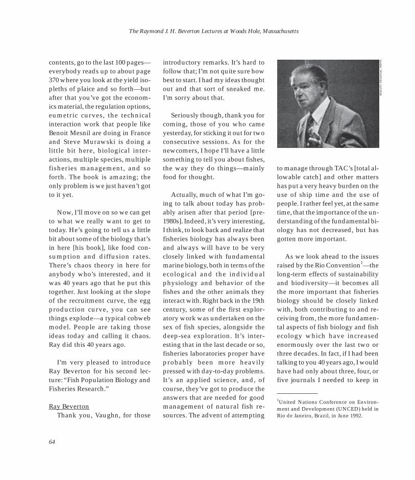
The Raymond J. H. Beverton Lectures at Woods Hole, Massachusetts
contents, go to the last 100 pages— everybody reads up to about page 370 where you look at the yield isopleths of plaice and so forth—but after that you’ve got the economics material, the regulation options, eumetric curves, the technical interaction work that people like Benoit Mesnil are doing in France and Steve Murawski is doing a little bit here, biological inter-actions, multiple species, multiple fisheries management, and so forth. The book is amazing; the only problem is we just haven’t got to it yet.
Now, I’ll move on so we can get to what we really want to get to today. He’s going to tell us a little bit about some of the biology that’s in here [his book], like food consumption and diffusion rates. There’s chaos theory in here for anybody who’s interested, and it was 40 years ago that he put this together. Just looking at the slope of the recruitment curve, the egg production curve, you can see things explode—a typical cobweb model. People are taking those ideas today and calling it chaos. Ray did this 40 years ago.
I’m very pleased to introduce Ray Beverton for his second lecture: “Fish Population Biology and Fisheries Research.”
Ray Beverton Thank you, Vaughn, for those
introductory remarks. It’s hard to follow that; I’m not quite sure how best to start. I had my ideas thought out and that sort of sneaked me. I’m sorry about that.
Seriously though, thank you for coming, those of you who came yesterday, for sticking it out for two consecutive sessions. As for the newcomers, I hope I’ll have a little something to tell you about fishes, the way they do things—mainly food for thought.
Actually, much of what I’m going to talk about today has probably arisen after that period [pre-1980s]. Indeed, it’s very interesting, I think, to look back and realize that fisheries biology has always been and always will have to be very closely linked with fundamental marine biology, both in terms of the ecological and the individual physiology and behavior of the fishes and the other animals they interact with. Right back in the 19th century, some of the first exploratory work was undertaken on the sex of fish species, alongside the deep-sea exploration. It’s interesting that in the last decade or so, fisheries laboratories proper have probably been more heavily pressed with day-to-day problems. It’s an applied science, and, of course, they’ve got to produce the answers that are needed for good management of natural fish re-sources. The advent of attempting
to manage through TAC’s [total allowable catch] and other matters has put a very heavy burden on the use of ship time and the use of people. I rather feel yet, at the same time, that the importance of the understanding of the fundamental biology has not decreased, but has gotten more important.
As we look ahead to the issues raised by the Rio Convention1—the long-term effects of sustainability and biodiversity—it becomes all the more important that fisheries biology should be closely linked with, both contributing to and receiving from, the more fundamental aspects of fish biology and fish ecology which have increased enormously over the last two or three decades. In fact, if I had been talking to you 40 years ago, I would have had only about three, four, or five journals I needed to keep in
1United Nations Conference on Environment and Development (UNCED) held in Rio de Janeiro, Brazil, in June 1992.
Mal
colm
Silv
erm
an, N
MFS
64

Lecture 2: Fish Population Biology and Fisheries Research
LIFE HISTORY STRATEGY
1. BROAD CONCEPT—Rationalizing natural history in terms of staying alive long enough to breed successfully for the next generation, i.e., satisfies the Euler-Lotka equation for stability:
λ
where Σ e−rtltmt = 1 t = 0
r = intrinsic rate of increase
lt = probability of survival to age t m = production of female offspring at age t
2. DEMOGRAPHIC INTERPRETATION
L.C. Cole (1954)G.C. Williams (1957)A. Comfort (1955–65)
Reproductive Strategy Population Ecology
Spawning PearlEggs Hatch MacArthurLarvae Metamorphosis SouthwardJuveniles Maturation FenchelAdults May
Growth r/K hypothesisMortality Foraging theoryMaturation EnergeticsFecundity Predator/preyLongevity
Figure 1. The broad concept and demographic interpretation of the life history strategy of fish.
touch with everything, and per-haps two or three dozen people around the world, the Bill Rickers and so forth, of that type. Now it’s almost impossible for any one per-son to keep up with the relevant information that is standing about on fish stocks and fish biology. It’s spread over a whole host of jour
nals, not just in the fisheries world, but outside. So, I must apologize, in a way, that I can only give you possibly a rather narrow look at fish.
However, the theme I’m thinking of for today is what has come to be called life history strategy.
Now that, to me, is almost another way of saying simply how best to get through the problems of living, reproducing, and producing the next generation. It embraces almost every aspect of ecology and biology. I think we have to narrow that down somewhat.
Let me just start then to put us in the picture, as it were, of the overall context of that which I’ve been exploring aspects (Fig. 1). Rationalizing natural history in terms of saying, “I’ve got enough to breed success over the next generation.” If you want to put it in mathematical terms, it would satisfy the Euler-Lotka equation of stability, which is another way of saying that each adult has got to produce enough eggs to carry off against losses and mortality, at least to re-place themselves by one individual in the next generation. If that’s the case, then you have essentially a stable situation.
The demographic interpretation of that formal mathematical equation owes a lot to L. C. Cole and his classic paper in 1954, which is very interesting because it was written as a rebuttal to very severe criticisms by William Allee, the great American field ecologist who said that theoretical ecology was useless. Having been stung by that criticism, Cole wrote what was to become the classic in setting down the framework for producing a the-
65
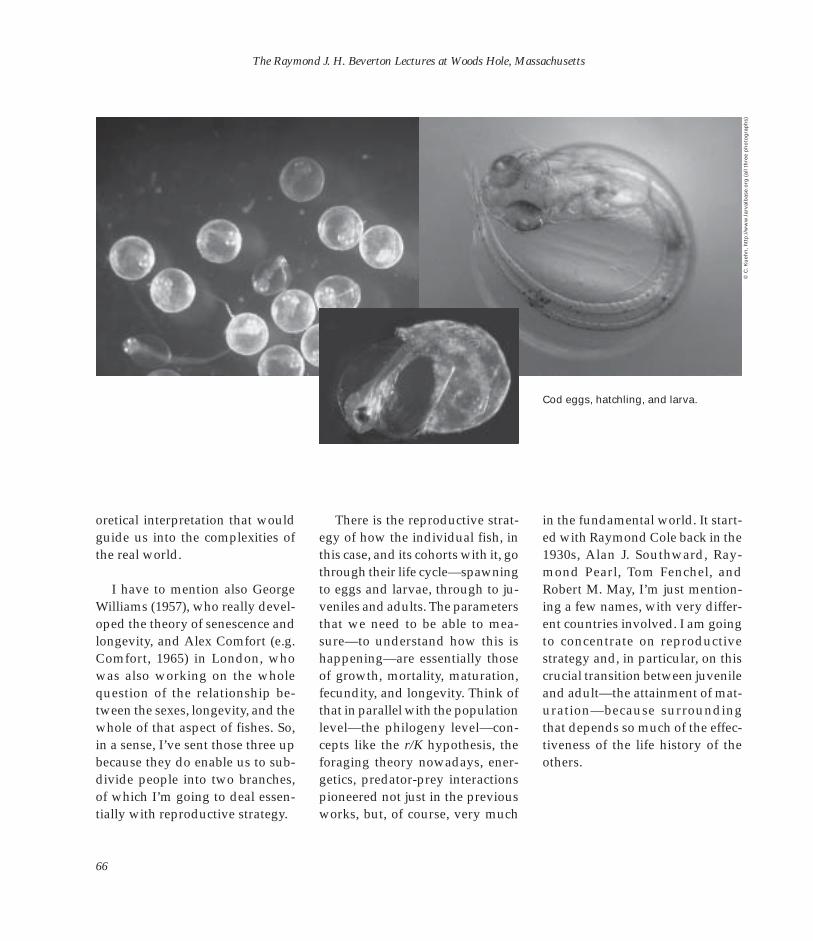
The Raymond J. H. Beverton Lectures at Woods Hole, Massachusetts
Cod eggs, hatchling, and larva.
© C
. Ku
ehn
, htt
p://
ww
w.la
rval
bas
e.o
rg (
all t
hre
e p
ho
tog
rap
hs)
oretical interpretation that would guide us into the complexities of the real world.
I have to mention also George Williams (1957), who really developed the theory of senescence and longevity, and Alex Comfort (e.g. Comfort, 1965) in London, who was also working on the whole question of the relationship be-tween the sexes, longevity, and the whole of that aspect of fishes. So, in a sense, I’ve sent those three up because they do enable us to sub-divide people into two branches, of which I’m going to deal essentially with reproductive strategy.
There is the reproductive strategy of how the individual fish, in this case, and its cohorts with it, go through their life cycle—spawning to eggs and larvae, through to juveniles and adults. The parameters that we need to be able to measure—to understand how this is happening—are essentially those of growth, mortality, maturation, fecundity, and longevity. Think of that in parallel with the population level—the philogeny level—concepts like the r/K hypothesis, the foraging theory nowadays, energetics, predator-prey interactions pioneered not just in the previous works, but, of course, very much
in the fundamental world. It started with Raymond Cole back in the 1930s, Alan J. Southward, Raymond Pearl, Tom Fenchel, and Robert M. May, I’m just mentioning a few names, with very different countries involved. I am going to concentrate on reproductive strategy and, in particular, on this crucial transition between juvenile and adult—the attainment of maturation—because surrounding that depends so much of the effectiveness of the life history of the others.
66

Lecture 2: Fish Population Biology and Fisheries Research
Before we get into too much de-tail, I expect you’ve seen the mate-rial in Figure 2 before. It’s from a paper by Gross, Coleman, and McDowall in 1988 which I find to be one of the more encouraging pieces of evidence to suggest that there really is a rationale between the way animals do things. They showed that the number of anadromous, compared with catadromous, species varies systematically with latitude. The anadromous ones, that is, the ones that are born and spawn in the freshwater and go down to the sea to grow up, are much more abundant in the high latitudes, and vice versa. They showed that this was because the productivity in freshwater is very limited and poor in the northern high latitudes. So, to grow up effectively and fast, they have to go down to the sea. Whereas, conversely, in the tropics, freshwater is more productive, and the sea is less so. The general question of how you should arrange your whole reproductive life in accordance with where you live does make sense.
Figure 2. Diadromy and productivity. A: Number of anadromous and catadromous species by latitude. B: Primary productivity of sea and freshwater by latitude. C: Percentage anadromy vs. ocean/freshwater productivity. Figures redrawn from Gross et al. (1988).
An
adro
mo
us
fish
sp
ecie
s (%
) N
um
ber
of
fish
sp
ecie
s
50
40
30
20
10
0
Catadromy Anadromy
A
0–5 10–15 20–25 30–35 40–45 50–55 60–65 70–75
(Equatorial) (Polar) Latitude (5A intervals)
1000
800
600
400
200
0
2
3
10
1 1
5 8
26
15
26 16
8 7 6
Freshwater Ocean
B
0–5 10–15 20–25 30–35 40–45 50–55 60–65 70–75
(Equatorial) (Polar) Latitude (5A intervals)
100
80
60
40
20
0
–1.2 –0.8 –0.4 0 0.4 0.8 1.2
12.5
7.5
2.5 22.5
27.5
32.5
37.5
42.5 52.5 47.5
57.5 62.5
72.5
67.5
Freshwater>ocean Freshwater<ocean
C
Log (ocean/freshwater) productivity
Prim
ary
pro
du
ctiv
ity
(car
bo
n, g
/m2 /y
ear
67
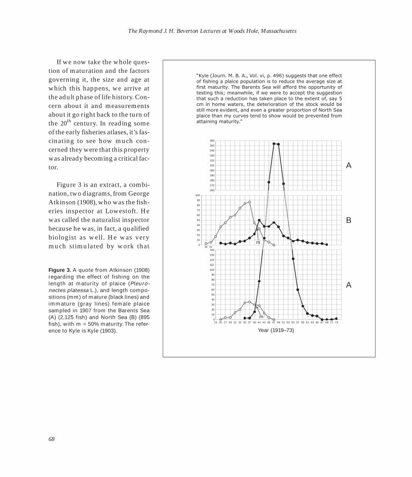
The Raymond J. H. Beverton Lectures at Woods Hole, Massachusetts
If we now take the whole question of maturation and the factors governing it, the size and age at which this happens, we arrive at the adult phase of life history. Concern about it and measurements about it go right back to the turn of the 20th century. In reading some of the early fisheries atlases, it’s fascinating to see how much concerned they were that this property was already becoming a critical factor.
Figure 3 is an extract, a combination, two diagrams, from George Atkinson (1908), who was the fisheries inspector at Lowestoft. He was called the naturalist inspector because he was, in fact, a qualified biologist as well. He was very much stimulated by work that
Figure 3. A quote from Atkinson (1908) regarding the effect of fishing on the length at maturity of plaice (Pleuronectes platessa L.), and length compositions (mm) of mature (black lines) and immature (gray lines) female plaice sampled in 1907 from the Barents Sea (A) (2,125 fish) and North Sea (B) (895 fish), with m = 50% maturity. The reference to Kyle is Kyle (1903).
25 27 29 31 33 35 37 39 41 43 45 47 49 51 53 55 57 59 61 63 65 67 69 71 73
360
350
340
330
320
310
300
290
280
270
260
100
90
80
70
60
50
40
30
20
10
0 19 21
130
120
110
100
90
80
70
60
50
40
30
20
10
0
140
23
Year (1919–73)
“Kyle (Journ. M. B. A., Vol. vi, p. 496) suggests that one effect of fishing a plaice population is to reduce the average size at first maturity. The Barents Sea will afford the opportunity of testing this; meanwhile, if we were to accept the suggestion that such a reduction has taken place to the extent of, say 5 cm in home waters, the deterioration of the stock would be still more evident, and even a greater proportion of North Sea plaice than my curves tend to show would be prevented from attaining maturity.”
m
m
A
B
A
68
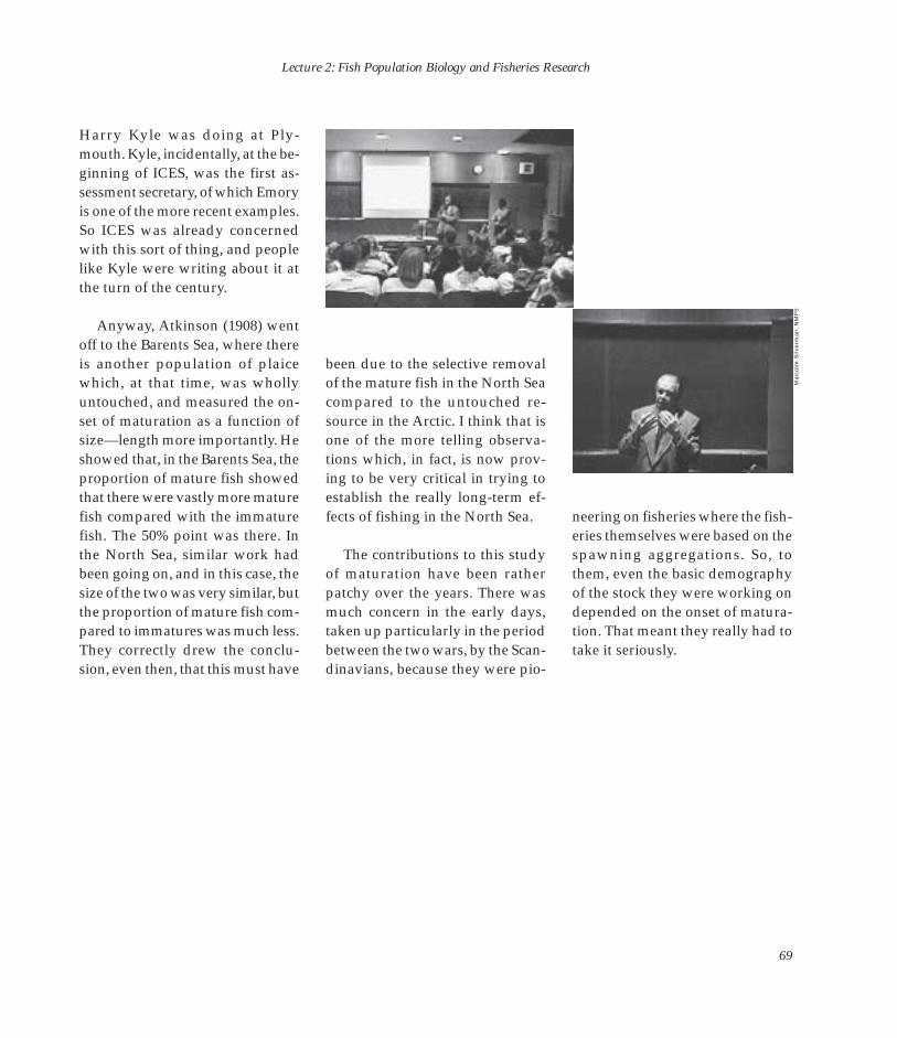
Lecture 2: Fish Population Biology and Fisheries Research
Harry Kyle was doing at Ply-mouth. Kyle, incidentally, at the be-ginning of ICES, was the first assessment secretary, of which Emory is one of the more recent examples. So ICES was already concerned with this sort of thing, and people like Kyle were writing about it at the turn of the century.
Anyway, Atkinson (1908) went off to the Barents Sea, where there is another population of plaice which, at that time, was wholly untouched, and measured the on-set of maturation as a function of size—length more importantly. He showed that, in the Barents Sea, the proportion of mature fish showed that there were vastly more mature fish compared with the immature fish. The 50% point was there. In the North Sea, similar work had been going on, and in this case, the size of the two was very similar, but the proportion of mature fish compared to immatures was much less. They correctly drew the conclusion, even then, that this must have
been due to the selective removal of the mature fish in the North Sea compared to the untouched re-source in the Arctic. I think that is one of the more telling observations which, in fact, is now prov-
Mal
colm
Silv
erm
an, N
MFS
ing to be very critical in trying to establish the really long-term effects of fishing in the North Sea.
The contributions to this study of maturation have been rather patchy over the years. There was much concern in the early days, taken up particularly in the period between the two wars, by the Scandinavians, because they were pio
neering on fisheries where the fisheries themselves were based on the spawning aggregations. So, to them, even the basic demography of the stock they were working on depended on the onset of maturation. That meant they really had to take it seriously.
69
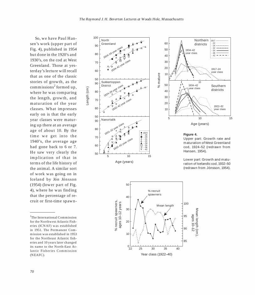
The Raymond J. H. Beverton Lectures at Woods Hole, Massachusetts
So, we have Paul Hansen’s work (upper part of Fig. 4), published in 1954 but done in the 1920’s and 1930’s, on the cod at West Greenland. Those at yesterday’s lecture will recall that as one of the classic stories of growth, as the commissions2 formed up, where he was comparing the length, growth, and maturation of the year classes. What impresses early on is that the early year classes were maturing up there at an average age of about 10. By the time we get into the 1940’s, the average age had gone back to 6 or 7. He saw very clearly the implication of that in terms of the life history of the animal. A similar sort of work was going on in Iceland by Jón Jónsson (1954) (lower part of Fig. 4), where he was finding that the percentage of recruit or first-time spawn-
2The International Commission for the Northwest Atlantic Fisheries (ICNAF) was established in 1951. The Permanent Commission was established in 1953 for the Northeast Atlantic fisheries and 10 years later changed its name to the North-East Atlantic Fisheries Commission (NEAFC).
Figure 4.
Upper part: Growth rate and maturation of West Greenland cod, 1924–52 (redrawn from Hansen, 1954).
Lower part: Growth and maturation of Icelandic cod, 1932–50 (redrawn from Jónsson, 1954).
100
90
80
70
60
50 90
80
70
60
50 90
80
70
60
50
North Greenland
1924–29 year class
1934–42 year class
Sukkertoppen District
1924–26 year class
1932–42 year class
Nanortalik
1931–32 year class
1932–42 year class
1924 - 26 - 29 - 31 - 32 - 34 - 35 - 36 - 42
5 10 15
Age (years)
Len
gth
(cm
)
% r
ecru
it s
paw
ner
s,
ages
10–
12 y
ears
Year class (1922–40)
Mean
leng
th (cm
), ag
es 10–12
% recruit spawners
Mean length
1917 - 22 - 24 - 32 - 34 - 36 - 42
60
50
40
30
20
10
50
40
30
20
10
10
5 10 15
1934–42 year class
1917–24 year class
1934–42 year class
1922–32 year class
Southern districts
Northern districts
% m
atu
re
Age (years)
50
40
30
20
10
0 22 25 30 35 40
100
95
90
85
70

Lecture 2: Fish Population Biology and Fisheries Research
ers coming into the spawning fish- Percentage of recruit-spawners in age groups 7–14 years 100ery changed inversely with the av-90
erage length. In other words, there 80
appeared to be a connection be- 70 tween age and length already 60 beginning to be established. 50
40
In Norway, similarly, Gunnar 30
Rollefsen, a man whom I found to 20
be a very stimulating person to 10
work with, led some of the early 0
working parties which pre-dated the now, very well established ICES working groups. I had the privilege of being associated with one of the very first ones in the early 1950’s. He was the chairman of it and Director of Fisheries Re-
Perc
enta
ge
search in Norway at Bergen, and was a cod specialist. He had observed, during the pre-war period, when the emphasis in the Institute was on herring, the technique of distinguishing, from the otoliths of the fish, or, in the case of herring in the North Sea, the scales, the change in the spacing of the rings which measured the onset of maturity. I’ll come to that later on. There are some examples of the changes in the age at which fish were arriving into the spawning fishery. Hence (Fig. 5) he was able to calculate the percentage of first-time spawners and use this as a technique for predicting next year’s, and the year after’s, size composition of the spawning stock.
Now, after the war we see, and I myself feel a little responsible or
32 34 35 36 37 38 39 40 41 42 43 44 45 46 47 48 49 50 51 52 53
95 94 93 92 91 90 89 88 87 86 85 84 83
Len
gth
(cm
)
7
8
9
10
11
12 13
8
9
10
11
12 13
14
7
8
9
10
11
12
13
Skrei. Lofoten
Year (1932–53)
Mean lengths of age groups 8–13 years
33
32 33 34 35 36 37 38 39 40 41 42 43 44 45 46 47 48 49 50 51 52 53
Year (1932–53)
Figure 5. Growth and maturation in Northeast Arctic cod, 1932–53 (re-drawn from Rollefsen, 1954).
ashamed in a way that I didn’t spot at that time, how important this was going to be. We rather neglected the maturation work, and it wasn’t just in the U.K., but it was quite widespread. Even the Nor
wegians didn’t follow it up in a way they now wished they had. So, for quite a long time, fisheries science didn’t contribute much to this subject after the Second World War. But it was going ahead in other
71

The Raymond J. H. Beverton Lectures at Woods Hole, Massachusetts
NM
FS
fields, and it was not really until the 1970’s that the fundamental fish biologists and ecologists generally picked up the whole question of maturation, stimulated by Cole’s 1954 paper, in particular. People like Steve Stearns and Derrick Broadford at Montreal in the 1970’s and 1980’s began to really point to the importance of this sort of thing. But towards the end of the 1950’s, after Sidney Holt and I had done our book (Beverton and Holt, 1957), we were looking at this, not from a point of view of life history
Cod, Gadus morhua.
strategies, as we would now call it, but to find a way of trying to measure natural mortality rates, which has always been very difficult and for which there are very limited data. It seemed to us that there ought to be a link between the natural life expectancy of a species and its growth potential. There’s no point in dying long before you’ve reached the limit of your growth span, and there’s no point in reproducing vastly too early when you can leave it until later, or too late to make the best of what life span
and growth you have. So, we used this as a device to try to arrive at a shorthand way of getting more sense into the very limited demo-graphic data we had then. That led to our dimensionless approach, ratios of natural mortality to speed of completion of the growth curve, which was not picked up at the time at all by the academic world. In fact, it wasn’t until Larry Charnov, a few years ago, from Utah realized that it was this, and he’s taken it much further since then (Charnov, 1993).
72

Lecture 2: Fish Population Biology and Fisheries Research
I should mention, before I go on to this particular work which is a sequel to that, that the one person in the fish world who really did, in the post-war period, put the whole question of this on the map was Gunnar Alm, the Swedish fish biologist. He was concerned also, from an applied (not a life history) standpoint, with utilizing the very many lakes and rivers in Sweden to best advantage to grow up his trout. He wanted to make sure that he knew how to adjust the stocking levels, given the different maturation rates and growth rates. He really laid the groundwork for our modern understanding of the interactions between growth and maturation, at least in the trout species (Alm, 1959) and more widely.
In 1992, our Fisheries Society of the British Isles had a Symposium on Fish Life History Strategies. I was asked whether I could look again at the whole question of the relationship between length at age and maturity which Sidney and I had done at the end of the 1950’s, and I had done a bit on in the early 1960’s. It is sometimes a rather questionable exercise to go back to something you did a long time ago when you know there is a lot more data that has come on since to see whether it still holds up, and I did so with some trepidation. Some-what to my surprise and relief, it
did hold up and indeed, if any-thing, it’s enabled it to be seen more clearly. It was work published a couple of years ago now (Beverton, 1992).
I just need to remind you of these definitions (Fig. 6): length and age at first maturity (L m, T m), length at infinity (L∞) from the von Bertalanffy growth curve which is a very fundamental way of representing the growth of fishes, and its other parameter, K, the rate of curvature or how fast it gets up towards its asymptote, which you will appreciate is a very vital part of the tradeoff between growth and maturity. A characteristic maxi-mum age is often all you have in some limited data. The natural mortality rate would be ideal, but it’s a very difficult thing to measure. Sometimes we need an adult life span—that’s the difference be-tween the age at which they mature and the age at which they find the average characteristic maxi-mum size at age. We have the following ratios from those which are these dimensionless ratios which Charnov (1993) has taken so much further than we did: length at maturity over L∞, which is the proportion of the potential growth span of the species before maturation, and M/K, the ratio of these two vital rates, the rate of dying off, the rate of growing, and one or two variations on those.
Patterns of reproductive parameters
Symbols and definitions
Lm = Length at 50% maturity
L∞ = Asymptotic length (von Bertalanffy growth curve)
K = Rate of curvature of the von Bertalanffy growth curve
Tm = Age at 50% maturity
T = Characteristic maximax mum age
Tad = Adult life span
M = Instantaneous coefficient of natural mortality
Ratios (dimensionless)
Lm/L∞ = Proportion of potential growth span completed before maturation
M/K = Ratio of the two vital rate coefficients: mortality and growth
M/Tmax = v
M = v/Tmax
M/K = v/KTmax
Figure 6. Symbols and definitions associated with patterns of reproductive parameters.
73

The Raymond J. H. Beverton Lectures at Woods Hole, Massachusetts
Let’s just run through the evidence on the relationship between these essential parameters: length and age at maturation and maxi-mum values, in four groups. There are a lot more other data avail-able, but I want to concentrate on within-major-taxon-group com
parisons, so Clupeiformes is one (Fig. 7). In Figure 7A is the length at maturity against L∞, and in Figure 7B is age at first maturity against maximum age. In Figures 7C and 7D are the same relationships for Atlantic cod, Gadiformes—very tight relationships, in the case of
herring; rather less so in the case of cod. That difference between cod and herring is one of many differences which I keep coming across as we can now do comparative population biology between these two species from a very, very rich data base in both cases.
Figure 7. Lm vs. L∞ and Tm vs. Tmax in Clupeiformes and Gadiformes (redrawn from Beverton, 1992).
40
30
20
10
0 0 0 20 30 40
L m cm T m
ax (
year
s)
T m (years)
25
20
15
10
5
0 0 05
150
100
50
0 50
L m (cm)
T max
(ye
ars)
25
30
20
15
10
5
0
T m (years)
5 0
C. harengus harengus L. North Atlantic
C. harengus harengus L. Baltic Sea
C. pallasii Valenciennes North Pacific
C. pallasii Valenciennes White Sea
Sprattus sprattus L. North Sea and Bay of Biscay
Sardinops caerulea Girard California
Sardinia pilchardus Walbaum East Channel
Sardinella aurita Valenciennes Southwest Atlantic
Engraulis encrasicholus L. North Sea and Biscay
Engraulis ringens Jenyns Southeast Pacific
Cetengraulis mysticetus Günther Tropical Pacific
Gadus morhua L. North Atlantic
Gadus morhua L. Labrador
Gadus morhua L. White Sea
Gadus morhua L. Faroes
Gadus morhua L. Irish Sea
Gadus morhua L. Norwegian fjords
Gadus macrocephalus Tilerius Northeast Pacific
Gadus ogak Richardson Hudson Bay and North Atlantic
Boreogadus saida Lepechin Barents and Beaufort Seas
Trisopterus minutus L. West Scotland
Trisopterus esmarki Nilson North Sea
Clupeiformes
Gadiformes
A
C
0 0
1
1
1
B
D
L ∞ (
cm)
L ∞ (
cm)
74

Lecture 2: Fish Population Biology and Fisheries Research
Pleuronectiformes
250
200
A
40
150 30
100 20
50 10
0 0 0 50 100 0 5 10 15
B Solid = male, open = female, where both
are shown
Pleuronectes platessa L. North Sea
Hippoglossus platesoides Fabricius Northwest Atlantic
Reinhardtius hippoglossoides (Walbaum) Norwegian Sea
Hippoglossus hippoglossus L. North Atlantic
Hippoglossus stenolepis Schmidt North Pacific
Limanda ferruginea Storer Northwest Atlantic
Glyptocephalus cynoglossus L. Northwest Atlantic
Solea vulgaris Quensel North Sea
Eopsetta jordani Lockington Northeast Pacific
Lm (cm) Tm (years)
Sebastes spp.
60 4
1
2
2 4 3
3
55
1 6
7 7
6
C 100
50 80
40 60
30 40
20 20
10 0
1 1 2 2
4 5 4
3 3
7 7 6 6
Pacific species
Atlantic species
D 5
Solid = male, open = female, where both are shown
S. emphaeus Starks; Puget Sound (a small cave-dwelling species)
S. serranoides Eigenmann & Eigenmann; California
S. fasciatus Storer; Gulf of Maine
S. mentella Travin; Northwest Atlantic
S. mentella Travin; Barents Sea
S. alutus Gilbert; Northwest Pacific 1
S. brevispinnis Been; Northwest Pacific 2
S. flavidus Ayres; Northwest Pacific 3
S. pinniger Gill; Northwest Pacific 4
S. reedi Westrheim &Tsuyuki; Northwest Pacific 5
S. zacentrus Gilbert; Northwest Pacific 6
S. proriger Jordan & Gilbert; Northwest Pacific 7
0 10 20 0
0 10 20 30 40 50 Tm (years)
Lm (cm)
Figure 8. Lm vs. L∞ and Tm vs. Tmax in Pleuronectiformes and Sebastes spp. (redrawn from Beverton, 1992).
It is sufficient for this purpose coming up quite significantly. And, side. That length business is just just to show you there is a quite interestingly, a group that couldn’t because of the ease of labeling, but strong proportionality between be done before because there was it’s also, as we’ll see in a minute, these two pairs of parameters: nothing known about them, which because length is a more conservalength at age of maturity compared was Sebastes (Fig. 8C and 8D), very tive parameter than age. to maximum values. In Figure 8A long lived, but still conformed to and 8B is the flatfish, with the dif- giving the same, quite tight rela- How are we going to interpret ferences between the two sexes tionship, especially on the length what these very strong relation-
L ∞ (
cm)
L ∞ (
cm)
T max
(ye
ars)
T max
(ye
ars)
75

The Raymond J. H. Beverton Lectures at Woods Hole, Massachusetts
ships mean? I think this is where I need to just scurry through the very complicated and fascinating subject which goes into behavior very strongly as well as demography. That is, even if we stay with a strategy, as defined originally by Maynard Smith (1982), the theoretical ecologist at the University of Sussex. He wrote it this way (Fig. 9): “...a phenotype such that, if almost all individuals have that phenotype, no alternative phenotype can invade the population.” That means, take over, in terms of reproductive capacity, to become the dominant source of reproductive material. In my terms, as applied to reproductive demographic strategy, I like to think of it as a combination of reproductive parameters, such as those we’ve just been looking at, that satisfy the evolutionary stable strategy (ESS). But indeed, no other combination within the scope of that phenotype could produce a greater life-time reproductive output. That’s my definition. So, we are really very
much closer to the evolutionary considerations. That relates to what I was saying right at the beginning about the importance of the very long-term effects of fishing, be-cause here we are on a time scale long enough to be thinking in terms of at least aiding in the evolutionary change.
There is a nice little exercise that Derrick Roff at Montreal did. He showed (Roff, 1984) that there is a simple equation (Fig. 9) which enables you to predict the age and size at which a group of fish would reach their maximum biomass. He showed that is the requirement for evolutionary stable strategy, although he didn’t call it that, but that is, in fact, what it was. He de-rived that equation by differentiating the number at weight as a function of age. In fact, it’s the same equation that Sidney Holt (1958) developed, for different reasons, as a means of showing at what size to start catching a year class in order to get the maximum yield out
of it if you fish hard enough. In a sense, it’s this curve (Fig. 9), where numbers are coming down and weight is going up; the product of the two is the biomass, and it’s roughly where the two cross that is the size. It means, therefore, that if you can know the M/K ratio, you can predict the F max or Fopt, what-ever you want to call it, which optimizes or conforms to the evolutionary stable strategy. That shows that these parameters, mortality and growth, are so balanced that it is the best arrangement they can have to maximize their life-time productivity. Roff calculated the expected value of this (he called it Lopt, in terms of knowing what M and K were for various species), and it showed me you get a very close fit between the predicted length at first maturity against the observed one in a number of species. That’s what he did in Figure 9 (lower graphs).
Mal
colm
Silv
erm
an, N
MFS
76

Lecture 2: Fish Population Biology and Fisheries Research
Roff (1984) showed that the same equation also gives maximum life-time biomass per recruit and defined L max as Lopt.
Definition (Maynard Smith): “...a phenotype such that, if almost all individuals have that phenotype, no alternative phenotype can invade the population.”
As applied to reproductive (demographic) strategy (?): “...a combination of reproductive parameters satisfies ESS if no other combination within the scope of that phenotype could produce a greater life-time reproductive output.”
Holt (1958):
for maximum biomass:
Age
Numbers Biomass Weight
16
14
12
10
8
6
4
2
0 0 10 12 14 16
Pred
icte
d a
ge
at m
atu
rity
(ye
ars)
Observed age at maturity (years)
r = 0.78 n = 31 P < 0.001
80
100
60
40
20
0 0 0 40 60 0 100
r = 0.93 n = 31 P < 0.001
Pred
icte
d le
ng
th
at m
atu
rity
(cm
)
Observed length at maturity (cm)
Evolutionary Stable Strategy (ESS) Maynard Smith (1982)
Nu
mb
er a
nd
wei
gh
t
d(Nt •Wt)/dt = 0
L max = L∞[1/(1+M/3k)]
8 6 4 2 2 8
Figure 9. Definition and sup-porting examples for the evolutionary stable strategy (Maynard Smith, 1982).
77
The Raymond J. H. Beverton Lectures at Woods Hole, Massachusetts
I have never been able to quite find out exactly how Roff got all this data together because, in fact, there’s an M/K problem here as well as another, and it seems to be important to put the two together if we’re going to get a proper comprehensive statement. So what I did in Figure 10 was to plot the ratio of L m over L∞, up the left-hand side, against the product of K and maximum age. Maximum age and natural mortality are inversely re-
Mal
colm
Silv
erm
an, N
MFS
lated, as they are a first approximation. I actually used M/K, which gives a nice asymptotic theoretical curve. That’s the predicted range you should have to compare with how the data actually distribute themselves, using observed length at maturity compared to the predicted one. It’s only roughly, but bringing in the other parameters as well, it’s just a length problem. In fact, for the four groups, they did distribute themselves quite significantly (Figure 10D). Something clearly isn’t right and proper in here [plot for Sebastes]. Either the data or the parameters are wrongly estimated or the fish is not able to leave as strong as it should before it matures. But leaving that point aside, there is no doubt that there are some general envelopes which spread themselves out in that sort of direction. There is a clear dis
tinction between the Sebastes and the Clupeoids, whereas Pleuronectiformes and Gadiformes are indistinguishable.
All that I’ve been talking about is what you’d call statics of the story. These are established pat-terns, probably built up over evolutionary time, certainly over long periods. We take a snapshot of them, and then this is the pattern that emerges. But, that’s only part of the story because the next question is: What’s going to happen in time if a population is pressed, for some reason or other? That could be overfishing. Is it going to respond with its maturation at size and age, as those patterns that I’ve just shown you would predict? In other words, are the dynamics of maturation predictable from the statics of maturation?
Figure 10 (opposite page). Evolutionary stable strategy combination of growth, maturation, and longevity parameters and resulting plots for Clupeiformes, Gadiformes, Pleuronectiformes, and Sebastes spp. (redrawn from Beverton, 1992) using the following maximum life-time biomass equation: LESS/L∞ = 1/ (1+M/3K). See Figure 7 for keys to symbols for A and B, and Figure 8 for keys to symbols for C and D.
78

Lecture 2: Fish Population Biology and Fisheries Research
1.0
0.9
0.8
0.7
0.6
0.5
0.4
0.3
0.2
0.1
0 1
KT max
1.0
0.9
0.8
0.7
0.6
0.5
0.4
0.3
0.2
0.1
0 1
L m/L∞
KT max
1.0
0.9
0.8
0.7
0.6
0.5
0.4
0.3
0.2
0.1
0 1
L m/L∞
KT max
1.0 0.9 0.8 0.7 0.6 0.5 0.4 0.3 0.2 0.1
0 1 2 3 4 5 6 7 8
KT max
9 10 11 12 13 14 15
E M
1 1
2 2
2
33
4 5
5
6 7
7 S
0.9
0.8
0.7
0.6
0.5
0.4
0.3
0.2
0.1
0 2 3 4 10 11 12
L m/L∞
KT max
Pleuronectiformes Gadiformes Clupeiformes Sebastes spp.
Sebastes spp.
PleuronectiformesGadiformesClupeiformes
B C
D
E
8 7 6 5 4 3 2 7 6 5 4 3 2
6 5 4 3 2
1 9 8 7 6 5
A
L m/L∞
L m/L∞
79
The Raymond J. H. Beverton Lectures at Woods Hole, Massachusetts
Well, the answer is they are not. You may be not surprised to hear they are not. This is where we’re breaking into, at the least the data is not all that new, but I think putting it together like this is perhaps a little step further than certainly I’ve been able to get so far. Those of you who were with me yesterday will remember the story of the collapse of the Norwegian spring-spawning herring, a very dramatic event in the 1960’s. The solid line in Figure 11, SSB, is coming whist-ling down, and it’s taken a long, long time before finally, in the last 2–3 years with a few good year classes, it has come back up again. During that time [1960’s and early 1970’s], the measurements of age and length at maturity were not taken. This is where the Norwegians are kicking themselves for not getting this filled in. Not many others at the time realized the importance of it. There’s no doubt that L∞ was up right about 30 cm and age somewhere getting on to 6 years old—average age of maturity for the whole population. You
30 6
5
T m
L m
SSB
A 10
20 4
3
5
10 2
1
0 0 1950 1960 1970 1980 1990
Year class
Lm (1950–60)
Lm (1974)
35
30
25
20
15
10
5
T m(1974) T m(1950–60)
1974 year class
1950–60 year class B
40
0 5 10 15
Age (years)
Figure 11. Spawning stock biomass (SSB) and length and age at maturity (A), and length vs. age for the 1950–60 and 1974 year classes (B) of Norwegian spring-spawning herring. Data from Østvedt (1964), Dragesund et al. (1980), Toresen (1986, 1990), and ICES (1994).
L m (
cm)
m (
year
s)
SS
B (10
–6 t)
Len
gth
(cm
) T
80

Lecture 2: Fish Population Biology and Fisheries Research
can pick it up certainly by the mid-1970’s; it was coming in—it was way down to 31/2 years—but the length was hardly any different. In the meantime, it’s been coming back up. It’s not back up as far as it was, but then neither has the biomass built back up as far as it was. Nevertheless, there is quite a bit of reversibility in this.
Another point, of course, of importance that we need to know is reversibility. How far do these sort of changes, in fact, reverse. There’s some preliminary evidence for it in Figure 11. In fact, what was happening in the 1950’s and 1960’s and the 1974 year class, which was one of those growing up from a very reduced base, perhaps 1/200 of the population size compared to earlier, is that it’s growing up on a much, much steeper growth curve, and the shift in length at maturity was almost horizontal.
Figure 12 shows the Icelandic herring, which also collapsed and recovered much more strongly than the Norwegian. Again, the age at maturity is pitching right down (late 1960’s–early 1970’s), coming back up again to pretty well where it was, length at maturity calm and unruffled and hardly taking any notice of all these things going on, staying pretty well constant around about 25 cm while the population was busy coming back up again.
L m (
cm)
35
30
4
3
2
1
0
T m (years)
9
5
3
2
1
T m
N
L m
2600
2200 30 25
1800
1400 20
100020
600 10
200
015 0
60 62 64 66 68 70 72 74 76 78 80 82 84
Year
Figure 12. Changes in age (Tm) (heavy gray line) and length (Lm) (dotted gray line) at maturity of Icelandic herring compared with changes in mean length for 1, 2, 3, 5, and 9 ringed herring (thin solid lines) and total stock size in numbers (N ) (dashed line) from 1960 to 1983. Data from Jakobsson and Halldórsson (1984).
Mea
n le
ng
th (
cm)
Sto
ck size (nu
mb
ers Z 10–6)
81

The Raymond J. H. Beverton Lectures at Woods Hole, Massachusetts
So, I’ll try and see if I can put together some of this evidence from several other species which we have covered, starting with age and measuring the change in average age at maturity against the degree of stock depletion on the log scale (Fig. 13). Catch for each species, roughly represented by the heavy gray lines, is coming down. On the x-axis you can see half stock size and quarter stock size, and the various plots show what was happening to age at maturity. The heavy gray lines are very much odd fits which, nevertheless, are showing a pretty broad resemblance to catch, with one exception. The Nova Scotia cod data I had discarded first. It was data, I think, from Beacham’s (1983) study which had been savagely criticized, and I thought I’d probably better not use it. But then after a bit, I began to think maybe it’s not quite so funny as it seems when you compare that with these other species which are
T m (
year
s)Lo
ge
2.5
11
10
9
8
2.0 7
6
5
1.5
4
3
1.0
2
0.5
(1.1)
(1.0)
(0.9)
(0.8)
0
H. platessoides (North Atlantic)
H. hippoglossus (Norway)
M. aeglefinus (Northeast Arctic)
G. morhua (Northeast Arctic and Nova Scotia)
61–64 60
60 69–72
1950
1984
82
82 61–64
62–66 69–72
82–85
50–60
1973
80–89 1955? ?
62
71–74
1970 1980
60 1989
84 64
Cod (Northeast
Arctic)
Cod (Nova Scotia)
1 0.5 0 –0.5 –1.0 –1.5 –2.0 –2.5 –5.0
1/2 1/4 1/10 1/20
Loge relative stock depletion
Figure 13. Change in average age at maturity (Tm) for nine different fish stocks vs. the degree of stock depletion.
Tm
(years)
C. harengus (Norwegian spring spawning)
C. harengus (Icelandic)
S. scombrus (North Sea)
S. solea (North Sea)
82

Lecture 2: Fish Population Biology and Fisheries Research
56 similar, except for the possibility of
54 the later trend in the Arctic cod.
52 There wasn’t much happening during the early period for the Arc-
50 tic cod. But, we’ll see in a moment.
33
32 I’ve put [Nova Scotia cod] in
31 S. scombrus (North Sea) much more recently because may-
30 be it wasn’t quite so unreliable as it was made out to be. On the other
32 hand, the length changes (Fig. 14),
31 as you might expect from what I’ve
30 just been saying, were almost
29 undetectable, except again for cod.
G. aeglefinus (Northeast Arctic)
G. morhua (Nova Scotia)
C. harengus (Norway)
Mea
n le
ng
th a
t m
atu
rity
(L m
) (
cm)
28
29
28
27
26
29
28
27
26
25
C. harengus (Iceland)
That was really unexpected and, again, that’s really what made me wonder whether I should proceed with that figure. So, I’ve included it because I want to show you some more sharply defined evidence that was coming from this story. There’s a general picture of the very robust, very conservative
S. solea (North Sea) change in length, but a much sharper change in age at maturity in response to whatever reason, but mainly by fishing in these cases.
0.5 0 –0.5 –1.0 1.5 – –2.0 –2.5 –3.0
1/2 1/4
1/10 1/20
Loge relative stock depletion
Figure 14. Change in mean length at maturity (Lm) for six different fish stocks vs. the degree of stock depletion.
83
The Raymond J. H. Beverton Lectures at Woods Hole, Massachusetts
In fact, to summarize it, Figure 15 shows the percentage fall in T m and L m for a given halving of the stock biomass. They [stocks] all went sliding down the growth curve; the length is going off and staying up horizontally, even though the age is dropping, and it’s not coming down the growth curve like you would think if it had been in the same state. Nova Scotia cod had a very large change, not only in the age, which is remarkable, but in length as well.
Just to make that point just now, in Figure 16 are the growth curves that you’ll get if you had that relationship between L m and L∞. Right across the range of different species, the top two [Fig. 16A] are the Norwegian and Icelandic growth curves. That’s the maturation curve on the left that they should be coming down if they were right-evolutionary-established on the basis of that static pattern. They didn’t come down that way at all. They came up one side, keeping up almost the same length at maturity. Looked at in more detail [Fig. 16B], you can see how both the two her-rings, as their age at maturity fell, didn’t come down the interpopulation maturity envelope established by evolution. So here’s a
kcotS nillaF Tm
)%( nillaF Lm
)%( nillafdetcepxE Lm fi)%(
evruchtworgegarevano
gnirrehgninwaps-gnirpsnaigewroN 11 1 01–7
gnirrehgninwaps-remmuscidnalecI 7 5.0 4
lerekcamaeShtroN 91 1 51–01
elosaeShtroN 9 0 5
kcoddahcitcrAtsaehtroN 41 4 01–7
docaitocSavoN 95 23 34
Figure 15. Percentage fall in Tm and Lm per halving of stock biomass.
dynamic which is really not con-forming at all to the established evolutionary structure.
Now, the trouble is, to analyze this further presents considerable difficulties because really what we’re looking for is a tradeoff be-tween growth, maturation, longevity, and all the rest of it. But if you are only seeing the average change in the total average of the population, attempting to try to measure the natural mortality before the population began to be depleted and then after is a nearly impossible task. It’s so dominated, due to fishing as it was in those days, by a very high fishing mortality. So the natural mortality, which is a brutal thing to estimate in the best of times, is pretty well
impossible to try to do in these circumstances.
The real question of just how much did a decrease in average age actually shorten the lifespan, if it did at all, which is what it did in those established static patterns, is a pretty critical thing to know be-cause otherwise we may be very wrong in applying our same ideas of natural mortality rate to the population which has had its average age at maturity coming down the chart. There was, how-ever, a thought that we had that might open up this question, and that is going back to the Norwegian herring and cod. I mentioned briefly in passing a few minutes ago that Norwegians started in the early 1930’s to measure both the
84
Lecture 2: Fish Population Biology and Fisheries Research Le
ng
th (
cm)
Len
gth
(cm
)
40
35
30
25
20
15
10
5
0 0 1 2 3 4 5 6 7 8 9 10 11 12 13 14 15 16 17 18
Age (years)
Immature
Mature
L∞ = 37.5
Icelandic Norwegian36
30
25
L∞ = 20
35
Interpopulation maturity envelope
A
32
31
30
29
28
27
26
25
24
23
22
21
20
Interpopulation maturity envelope
Icelandic
Norwegian
B
1.5 2 2.5 3 3.5 4 4.5 5 5.5 6
Age (years)
age at which the fish matured as well as its maximum age in the fishery, and they had been using that for a short-term stock measure for both herring and cod, but they dropped that after the Second World War and didn’t use it. Well they did at first, but after the crash of herring anyway, they didn’t re-ally use the cod very much after that. So I said to Ole Johan Østvedt (who had used it very much in the 1950’s), and Arvid Hylen at Bergen,
Figure 16. Growth curves for varying values of L∞ ranging from 20 to 37.5 cm and showing the interpopulation maturity envelope (A), with an expanded portion (B) contrasting the theoretical curves with observed values of length at age for Icelandic and Norwegian herring.
85

The Raymond J. H. Beverton Lectures at Woods Hole, Massachusetts
“Why don’t we go back to the old 400
data set and work it up in a different way?” Ask the question, “Can 300
we see which fish mature from adifferent year class at age 6, 7, 8, 9,
20010?” In the case of cod (Beverton et al., 1994), this (Fig. 17A) is the distribution of the age at which 100
they matured. The cod is the shaded area and herring is the un- 100shaded area. You can see that the 3 4 5 6 7 8 9 10 11 12 13
1925–30 year classes A
Cohort maturation age (years)
8
6
4
2
0
–2 0 5 10 15 20
1933 year class MC-9 MC-10
MC-8
MC-7
MC-12
MC-13
B
Age (years)
Figure 17. A: Frequency distribution (per mille) of maturation cohorts (MC) of Northeast Arc-tic cod (1925–30 year classes; shaded area) and Norwegian spring-spawning herring (1933–37 year classes; unshaded area) at maturation. B: Loge CPUE vs. age of the maturation cohorts of the 1933 year class of Northeast Arc-tic cod.
Freq
uen
cy %
CP
UE
Log
e
86
14

Lecture 2: Fish Population Biology and Fisheries Research
range of the maturation in herring was between 3 and 9, and in cod it was from 6 to 14. Why have we worked them up on a cohort, maturation cohort? That is to say, “Well, let’s look at the fish that matured one year at 7 years old of the year class and see how many of those are left as 8 year olds the following year.” In other words, follow through an age composition based on a maturation cohort and ask then the question, “Can we see a difference in survival rate and growth rate between cohorts maturing from the same year class, but maturing at different ages?” There are, in fact, the age compositions of the 1933 year class of cod (Fig. 17B), the 7 year olds (they didn’t have enough 6’s to measure), the 8’s, the 9’s, 10’s, right on up to age 14. There isn’t a lot of difference in those spokes. There were more differences in some of the other year classes, but that’s the sort of thing I mean—splitting the year class up into its maturation cohorts. Of course, you dilute the data if you subdivide it again and again, and it gets much more difficult to make sure that you are re-ally seeing something. You’ve got to sort the scenarios out rather care-fully. But still, it was giving coherent results on the cod.
Mal
colm
Silv
erm
an, N
MFS
87
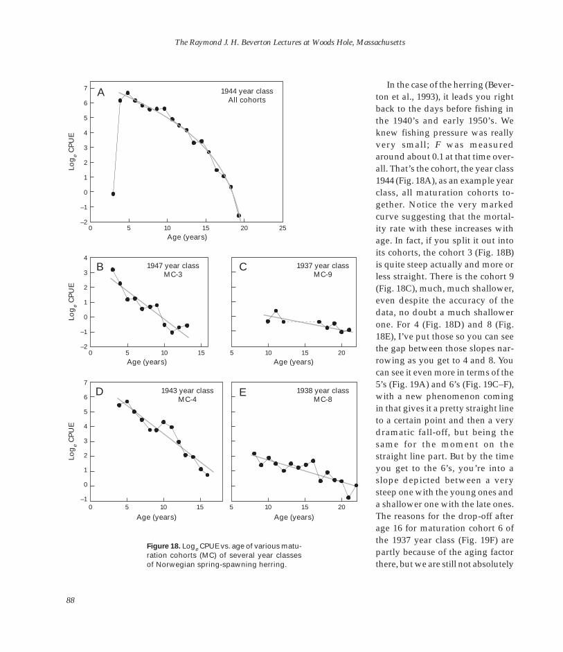
The Raymond J. H. Beverton Lectures at Woods Hole, Massachusetts
Log
e C
PU
ELo
ge
CP
UE
Log
e C
PU
E
7
6
5
4
3
2
1
0
–1
–2
4
3
2
1
0
–1
–2
7
6
5
4
3
2
1
0
–1
1944 year class All cohorts
A
0 5 10 15 20 25 Age (years)
0 10 10 15 20 5 15 Age (years) Age (years)
1947 year class MC-3
1943 year class MC-4
1938 year class MC-8
1937 year class MC-9
B C
D E
5
0 5 10 15 5 10 15 20
Age (years) Age (years)
Figure 18. Loge CPUE vs. age of various maturation cohorts (MC) of several year classes of Norwegian spring-spawning herring.
In the case of the herring (Beverton et al., 1993), it leads you right back to the days before fishing in the 1940’s and early 1950’s. We knew fishing pressure was really very small; F was measured around about 0.1 at that time over-all. That’s the cohort, the year class 1944 (Fig. 18A), as an example year class, all maturation cohorts together. Notice the very marked curve suggesting that the mortality rate with these increases with age. In fact, if you split it out into its cohorts, the cohort 3 (Fig. 18B) is quite steep actually and more or less straight. There is the cohort 9 (Fig. 18C), much, much shallower, even despite the accuracy of the data, no doubt a much shallower one. For 4 (Fig. 18D) and 8 (Fig. 18E), I’ve put those so you can see the gap between those slopes narrowing as you get to 4 and 8. You can see it even more in terms of the 5’s (Fig. 19A) and 6’s (Fig. 19C–F), with a new phenomenon coming in that gives it a pretty straight line to a certain point and then a very dramatic fall-off, but being the same for the moment on the straight line part. But by the time you get to the 6’s, you’re into a slope depicted between a very steep one with the young ones and a shallower one with the late ones. The reasons for the drop-off after age 16 for maturation cohort 6 of the 1937 year class (Fig. 19F) are partly because of the aging factor there, but we are still not absolutely
88

Lecture 2: Fish Population Biology and Fisheries Research
sure we’ve sorted out as much as the data would allow. An estimate is highly obtuse, but there is no doubt that some of this is very real. It’s, in fact, senescence, which has been detected, of course, in other species. But I hadn’t realized until we looked at this how marked it was in the herring, and it’s only possible to see it when you go back, such as we did here, to years where the level of fishing pressure was very small. The lifespan quite sharply finished at about age 23 or 24, irrespective of which cohort you’re talking about. There is a marked change in overall circumstances since this is mainly due as much to natural mortality. It means no doubt, in the case of herring, as far as we can see from this way of analyzing data, that the early maturers certainly had a much higher total mortality rate and probably, therefore, a higher natural mortality rate than did the late maturers. So here is evidence that if you mature young, you have a short life and a merry one, and if you leave it to later, you’ll have a much calmer, unruffled, but not very exciting life.
Log
e C
PU
ELo
ge
CP
UE
Log
e C
PU
E
5
4
3
2
1
0
–1
–2
1941 year class MC-5
A
5 10 15 20
Age (years)
6
5
4
3
2
1
0
–15 10 15 20
1938 year class MC-6
C
Age (years)
5 6
4 5
3 4
2 3
1 2
0 1
–1 0
–2 –1
–3 –2 7 10 15 20
1939 year class MC-6
E
Age (years)
1938 year class MC-7
B
5 10 15 20
Age (years)
1940 year class MC-6
D
5 10 15 20
Age (years)
1937 year class MC-6
F
7 10 15 20
Age (years)
Figure 19. Loge CPUE vs. age of various maturation cohorts (MC) of several year classes of Norwegian spring-spawning herring.
89

The Raymond J. H. Beverton Lectures at Woods Hole, Massachusetts
Now, we can also measure the growth parameters of each of these cohorts separately. So we’ve asked the question, “If you mature early, do you have a bigger K or longer L∞?” The answer is in the cod (Fig. 20A), except in the first two ages, the youngest. The 6’s and 7’s are not much different, they are rather below, but after that they’re pretty flat. In other words, it didn’t affect K or L∞, nor incidentally in the cod could we detect any real difference in slope of the survival curves. In other words, from about full maturity rate onwards, there seemed to be no difference in the natural mortality rate. That fit in with the fact that the growth parameters didn’t change either. Whereas in herring (Fig. 20B), L∞ stayed pretty flat, but the K, the parameter which should be much more closely related to natural mortality, came down quite sharply. In fact, our estimate of natural mortality from the age composition is even steeper—it may be too steep. We’re having to check whether that could possibly be a little shallower than that. It’s steeper than the drop in K in herring. There’s no doubt for both those that the change is different than in cod.
Kan
d M
K
and
M
150
0.2
100
0.1
0
Cod K
M
L∞
A
506 7 8 9 10 11 12 13 14
Cohort maturation age (years)
0.5
L∞
K
M
Herring B 45
0.4
40
0.3
35
0.2
30
0.1
0 25 2 3 4 5 6 7 8 9
Cohort maturation age (years)
Figure 20. Plots of K, M, and L∞ vs. cohort maturation age for Northeast Arctic cod (A) and Norwegian spring-spawning herring (B).
L∞ (cm
) L∞
(cm)
90
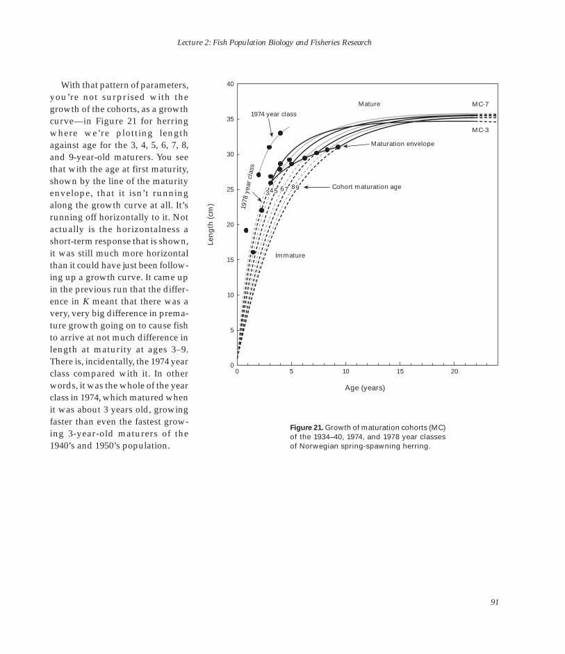
Lecture 2: Fish Population Biology and Fisheries Research
With that pattern of parameters, 40
you’re not surprised with the growth of the cohorts, as a growth curve—in Figure 21 for herring 35
where we’re plotting length against age for the 3, 4, 5, 6, 7, 8, and 9-year-old maturers. You see 30
that with the age at first maturity, shown by the line of the maturity
25envelope, that it isn’t running along the growth curve at all. It’s running off horizontally to it. Not
20actually is the horizontalness a short-term response that is shown, it was still much more horizontal
15than it could have just been following up a growth curve. It came upin the previous run that the differ-
10ence in K meant that there was avery, very big difference in premature growth going on to cause fish
5to arrive at not much difference inlength at maturity at ages 3–9.There is, incidentally, the 1974 year 0class compared with it. In other 0 5 10 15 20
words, it was the whole of the year Age (years)class in 1974, which matured whenit was about 3 years old, growing
Mature
1974 year class
1978
yea
r cl
ass
Maturation envelope
Cohort maturation age
Immature
MC-7
MC-3
3 5 6 7 8 9 4
faster than even the fastest grow-Figure 21. Growth of maturation cohorts (MC)
ing 3-year-old maturers of the of the 1934–40, 1974, and 1978 year classes 1940’s and 1950’s population. of Norwegian spring-spawning herring.
Len
gth
(cm
)
91
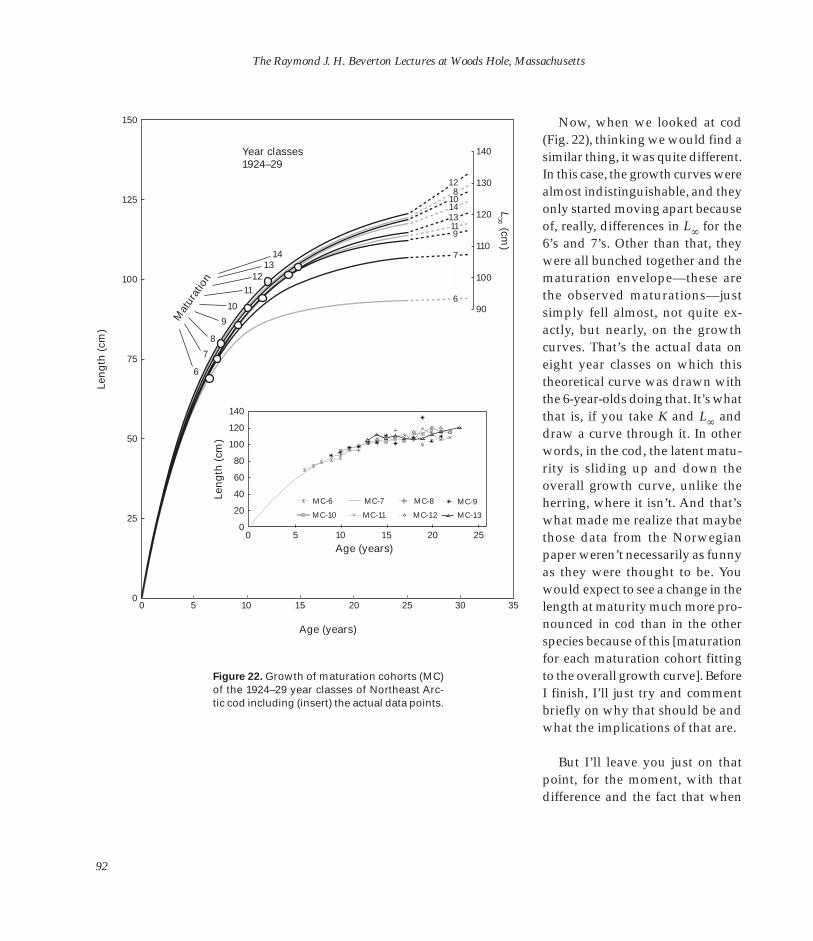
The Raymond J. H. Beverton Lectures at Woods Hole, Massachusetts
Len
gth
(cm
)
150
125
100
75
50
25
0 0 5 10 15 20 25 30 35
Year classes 1924–29
Len
gth
(cm
)
Age (years)
MC-6
MC-10
MC-7
MC-11
MC-8
MC-12
MC-9
MC-13
6
140
120
100
80
60
40
20
0 10 15 20 25 0
7
8
9
10
11 12
13 14
Mat
urat
ion
130
140
120
110
100
90 L∞
(cm)
13
9
7
6
11
12 8
10 14
5
Age (years)
Figure 22. Growth of maturation cohorts (MC) of the 1924–29 year classes of Northeast Arc-tic cod including (insert) the actual data points.
Now, when we looked at cod (Fig. 22), thinking we would find a similar thing, it was quite different. In this case, the growth curves were almost indistinguishable, and they only started moving apart because of, really, differences in L∞ for the 6’s and 7’s. Other than that, they were all bunched together and the maturation envelope—these are the observed maturations—just simply fell almost, not quite exactly, but nearly, on the growth curves. That’s the actual data on eight year classes on which this theoretical curve was drawn with the 6-year-olds doing that. It’s what that is, if you take K and L∞ and draw a curve through it. In other words, in the cod, the latent maturity is sliding up and down the overall growth curve, unlike the herring, where it isn’t. And that’s what made me realize that maybe those data from the Norwegian paper weren’t necessarily as funny as they were thought to be. You would expect to see a change in the length at maturity much more pronounced in cod than in the other species because of this [maturation for each maturation cohort fitting to the overall growth curve]. Before I finish, I’ll just try and comment briefly on why that should be and what the implications of that are.
But I’ll leave you just on that point, for the moment, with that difference and the fact that when
92

Lecture 2: Fish Population Biology and Fisheries Research
you superimpose those ages and 150
lengths at maturity on the staticpattern I’ve showed you, in thecase of the cod (Fig. 23A), thestraight line comes from the wholeof the Gadiformes that I showed inFigure 7. That’s superimposing L∞
100
and L m for the different cohorts. Inthe first two or three, they’re on theline, and after that they drop off to
9 11 13
6
7
8 10
12
14
Maturation cohorts age 6–14 years
Cod
A
50
3 47
9 568
Maturation cohorts age 3–9 years
Herring
B
0 0 50 100 150
L m (cm)
50
40
30
20
10
0 0 10 20 30 40 50
Lm (cm)
Figure 23. Lm vs. L∞ for maturation cohorts age 6–14 years for Northeast Arctic cod (A) and 3–9 years for Norwegian spring-spawning herring (B) contrasted with the static pattern (straight line) for each species.
the right. In the herring (Fig. 23 B), it’s also bunched up and it’s very much less steep than the overall, between-species, three population comparisons. So not only do we have a dynamic response which is very different from the static, but we have also, within one and the same population and within one and the same year class, a distance which is not conforming between the ages of the maturation cohorts, and which is not conforming to the overall pattern.
Now, can we, however, use this evidence to ask the question, “What is it that is sustaining that range of maturation and size and age in those two populations?” Could we have asked the question, “Is this an evolutionary stable arrangement? Why don’t those awful cod start maturing at age 6 or leave it until 14? Why do all the herring start maturing at age 3 or why don’t they all leave it to 9?” They’re capable of doing so. The potential to do so is there in the year class.
L ∞ (
cm)
L ∞ (
cm)
93

The Raymond J. H. Beverton Lectures at Woods Hole, Massachusetts
LIFETIME BIOMASS PER RECRUIT AT MATURITY
3
SSB = RmqL3 • 1/M Σ Un(1−Lm/L∞)
∞ n = 0 1 + (nK)/M
If fished with fishing mortality rate F:
3
SSB = RmqL3 • 1/M Σ Un(1−Lm/L∞)
∞ n = 0 1 + F/M + (nK)/M
This is an equilibrium statement. If Tm changes, then so may Lm/L∞, K, and possibly M. Furthermore, an extra multiplier is needed to adjust change in number of fish reaching maturity:
if Tm2 >/Tm1 ; e−M1 (Tm2 −Tm1)
if Tm2 >/Tm1 ; e−M2 (Tm1 −Tm2)
Figure 24. Equations for lifetime biomass per recruit at maturity.
Well, to answer this question we can do a simple calculation (Fig. 24). We can ask, “What is the life-time biomass?” It would be nice to be able to do a weekly age production, but I don’t have maturity data for each of these cohorts. There is overall maturation data for the her-ring, but nobody has ever done it on a maturation cohort yet. It would be easy enough to do, but it hasn’t been done. But we can do it
in terms of biomass and ask the question, “Is the lifetime biomass produced by each of these cohorts reaching its maximum point?” Does that give us a clue, because if it’s conforming to the evolutionarily stable principle, it should be reaching its maximum point. The maximum lifetime production is best on the interquartile range. I’ve just put up Figure 24 to remind you that it is rather fascinating that the
simple biomass equation is, in fact, the product of or involves these crucial ratios, M/K, and it is what makes that an interesting situation too. So, the whole spawning biomass per recruit derived in that equation can be written in purely dimensionless terms.
But, bringing these same ratios together, when you use that calculation for cod and herring, the dotted line in Figure 25 is the lifetime biomass per recruit arriving at maturity and, of course, of the fish arriving at maturity, which has to take any account of mortality losses in weight while immature. Then the later you mature, the better the biomass. However, if you ask the question for cod (Fig. 25A), you arrive at 6 years old, and you now have a choice: either mature at age 6 or wait until some later age to mature. If you wait until some later age, you’ll have to suffer a mortality rate in the process. So, although you’ll get a better lifetime biomass per numbers of eggs spawned if you survive to that age, you may not survive. If you put that into the equation using the rather limited range of mortality that we have, because we don’t re-ally know what the overall level is, 0.1 or 0.15 or 0.2, there are three curves shown. But in each case, though, there is an intermediate maximum, much stronger with curves (a) and (b) than with curve (c) which has a rather high natural
94
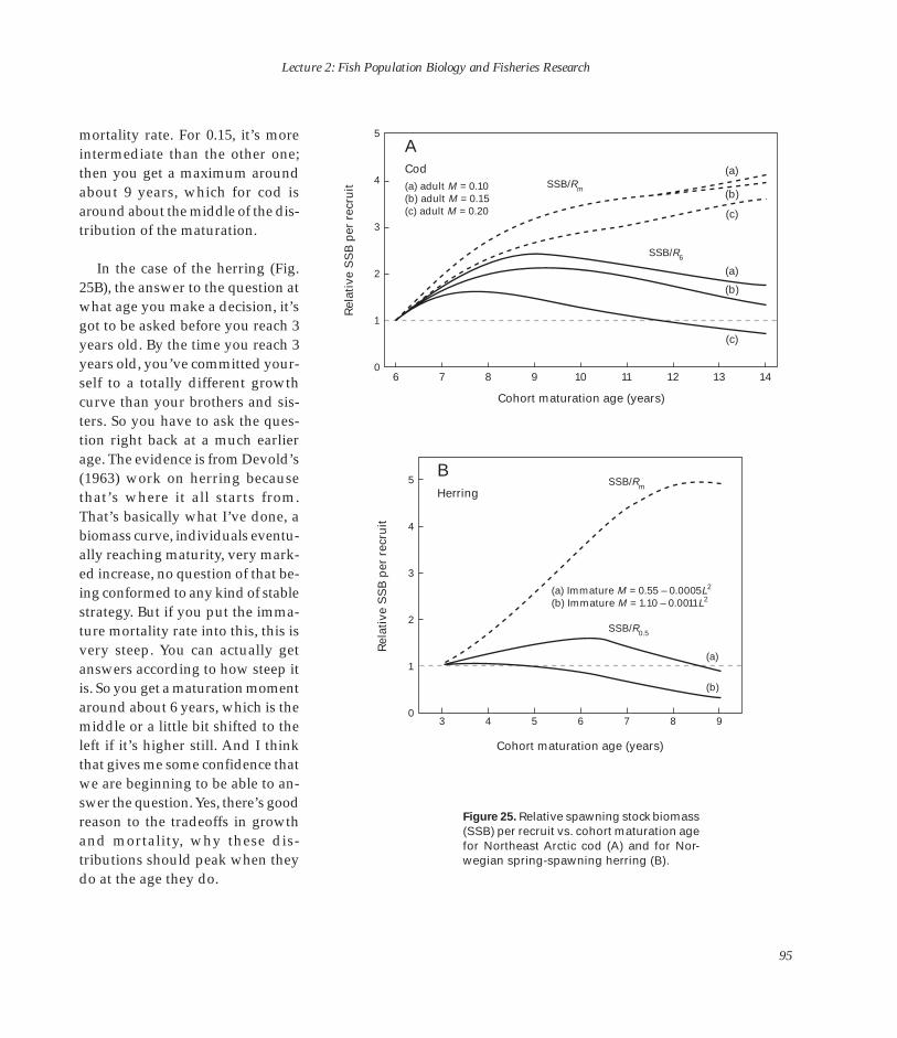
Lecture 2: Fish Population Biology and Fisheries Research
mortality rate. For 0.15, it’s more 5
intermediate than the other one;then you get a maximum around 4about 9 years, which for cod isaround about the middle of the distribution of the maturation.
In the case of the herring (Fig. 25B), the answer to the question at what age you make a decision, it’s got to be asked before you reach 3 years old. By the time you reach 3 years old, you’ve committed your-self to a totally different growth curve than your brothers and sisters. So you have to ask the question right back at a much earlier age. The evidence is from Devold’s (1963) work on herring because that’s where it all starts from. That’s basically what I’ve done, a biomass curve, individuals eventually reaching maturity, very marked increase, no question of that being conformed to any kind of stable strategy. But if you put the immature mortality rate into this, this is very steep. You can actually get answers according to how steep it is. So you get a maturation moment around about 6 years, which is the middle or a little bit shifted to the left if it’s higher still. And I think that gives me some confidence that we are beginning to be able to answer the question. Yes, there’s good reason to the tradeoffs in growth and mortality, why these distributions should peak when they do at the age they do.
Rel
ativ
e S
SB
per
rec
ruit
Rel
ativ
e S
SB
per
rec
ruit
(a) adult M = 0.10 (b) adult M = 0.15 (c) adult M = 0.20
Cod SSB/R m
SSB/R6
(a)
(b)
(c)
(a)
(b)
(c)
A
3
2
1
0 6 7 8 9 10 11 12 13 14
Cohort maturation age (years)
5
4
3
2
1
0 3 4 5 6 7 8 9
(a) Immature M = 0.55 – 0.0005L2
(b) Immature M = 1.10 – 0.0011L2
Herring SSB/R m
SSB/R0.5
(a)
(b)
B
Cohort maturation age (years)
Figure 25. Relative spawning stock biomass (SSB) per recruit vs. cohort maturation age for Northeast Arctic cod (A) and for Norwegian spring-spawning herring (B).
95

The Raymond J. H. Beverton Lectures at Woods Hole, Massachusetts
L m/L∞
an
d L
op
t/L∞
110
100
90
80
70
60 6 7 8 9 10 11 12 13 14 15 16
M = 0.1
M = 0.15
M = 0.2
L m A
Maturation cohort age (years)
1.0
0.9
0.8
0.7
0.6
0.5 0.5 1.0 1.5 2.0
M = 0.2
M = 0.15
M = 0.1
Lopt/L∞
B
K/M
Figure 26. Lm at each maturation cohort (age in years) (A) and Lm/L∞ vs. K/M (B) at three levels of natural mortality (M) for Northeast Arctic cod.
L an
d L
op
t (cm
)m
In fact, in the cod—I haven’t done this for herring yet—we can actually go back to that plot of L m/ L∞ against maturation age (Fig. 26A). For the different natural mortalities, 0.15 conforms most closely with the observed curve. Similarly, plotting those ratios against K/M (Fig. 26B), it’s again M = 0.15 that fits the observed curve much, much closer. So, it rather suggests there may indeed be a way here of distinguishing which level of natural mortality is the most realistic one. In that case, it would be 0.15.
Well, that really stands out as a method of estimating mortality. I think we’ll have to leave it until more work is done to be sure about it. It’s a rather intriguing possibility.
Now, just to finish up with a few concluding remarks to try and bring this back to the more general biological scene. I mentioned in the herring that there was evidence of this cohort distinction. It began to be noticeable much earlier in life that we saw them come to maturation. Figure 27 is from Lambert’s (1984) work on Nova Scotian her-ring, and it shows growth curves of cohorts from that coming through and staying distinct and producing length compositions in which you can see modes—in other words, from the very early stages of life history, the embryonic
96
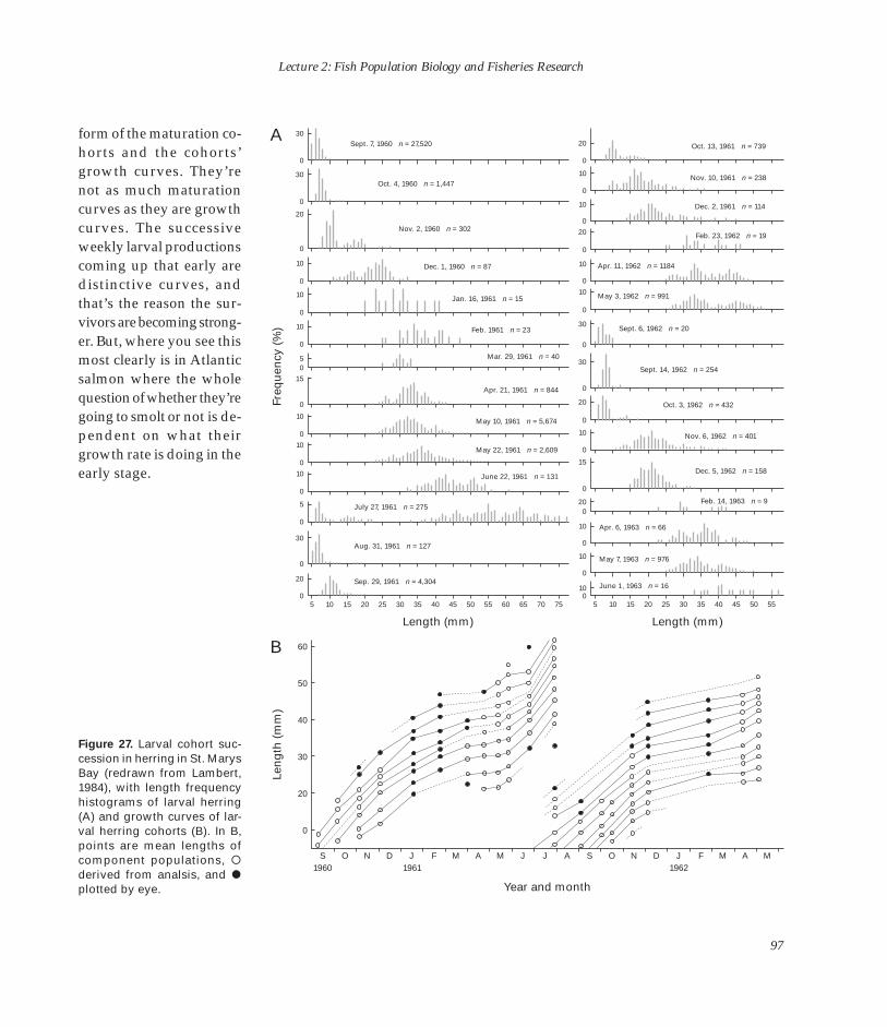
97
Lecture 2: Fish Population Biology and Fisheries Research
form of the maturation co-horts and the cohorts’growth curves. They’renot as much maturationcurves as they are growthcurves. The successiveweekly larval productionscoming up that early aredistinctive curves, andthat’s the reason the sur-vivors are becoming strong-er. But, where you see thismost clearly is in Atlanticsalmon where the wholequestion of whether they’regoing to smolt or not is de-pendent on what theirgrowth rate is doing in theearly stage.
Figure 27. Larval cohort suc-cession in herring in St. MarysBay (redrawn from Lambert,1984), with length frequencyhistograms of larval herring(A) and growth curves of lar-val herring cohorts (B). In B,points are mean lengths ofcomponent populations, �derived from analsis, and �plotted by eye.
30
0
30
0
20
0
10
0
10
0
10
0
15
0
10
0
10
0
10
0
5
0
30
0
20
0
20
0
10
0
10
0
20
0
10
0
10
0
30
0
30
0
20
0
10
0
15
0
200
10
0
10
0
100
50
5 0 15 20 25 30 5 0 5 0 5 0 5 0 5 5 0 15 20 25 0 5 0 5 0 5
Sept. 7, 1960 n = 27,520 Oct. 13, 1961 n = 739
Nov. 10, 1961 n = 238
Dec. 2, 1961 n = 114
Feb. 23, 1962 n = 19
Apr. 11, 1962 n = 1184
May 3, 1962 n = 991
Sept. 6, 1962 n = 20
Sept. 14, 1962 n = 254
Oct. 3, 1962 n = 432
Nov. 6, 1962 n = 401
Feb. 14, 1963 n = 9
Apr. 6, 1963 n = 66
May 7, 1963 n = 976
June 1, 1963 n = 16
Dec. 5, 1962 n = 158
Oct. 4, 1960 n = 1,447
Nov. 2, 1960 n = 302
Dec. 1, 1960 n = 87
Jan. 16, 1961 n = 15
Mar. 29, 1961 n = 40
Apr. 21, 1961 n = 844
May 10, 1961 n = 5,674
May 22, 1961 n = 2,609
June 22, 1961 n = 131
July 27, 1961 n = 275
Aug. 31, 1961 n = 127
Sep. 29, 1961 n = 4,304
Feb. 1961 n = 23
Length (mm)
Len
gth
(m
m)
Year and month
60
50
40
30
20
0
S N1960 1961 1962
D F M A AM J S O N D J F A M
A
B
Freq
uen
cy (
%)
Length (mm)
1 3 4 4 5 5 6 6 7 7 1 3 3 4 4 5 5
O J J M

The Raymond J. H. Beverton Lectures at Woods Hole, Massachusetts
40
20 9 June
30
27 June
10
30
10
25 July
30
Figure 28 shows early hatching salmon larvae just in a single mode, then beginning to develop within a couple of weeks into two modes, more still during the summer, and before long there is the group of smolts that go down the river (shaded area) and the group that stays behind (unshaded area). Some of those become precocious males—John Thorpe3 doesn’t like calling them precocious males— but they actually stay back and mature within a year or two at this size. Hence, it drives the tradeoff
Freq
uen
cy (
%)
22 August between staying as a precocious 10 male or having to deal with the
problem of dominant males com-30
9 September
ing back from the sea, of course, risking lots of mortality on the way,
10 but then having the females, as it were, under his own control and
30 29 September
able to ensure that the larger pro-portion of the fertilization came
10 from him, whereas the little ones have to sneak in and do the best they can. The tradeoff between the
30 efficiency of the fertilization and the more terrifying choice between
10 staying in the river, where you’d
4 6 8 10 do rather well in that case, or go-
Length (cm) ing down to sea, almost balances. In other words, the evolutionary stable strategy.
8 November
Figure 28. Salmonid developmental variation. Length-frequency distributions showing the progressive segregation of non-smolting (unshaded) and potential smolting (shaded) individuals of a population of age 0 Atlantic salmon (redrawn from Thorpe, 1989). 3John E. Thorpe, Freshwater Fisheries
Laboratory, Pitlochry, Perthshire, Scotland, U.K.
98
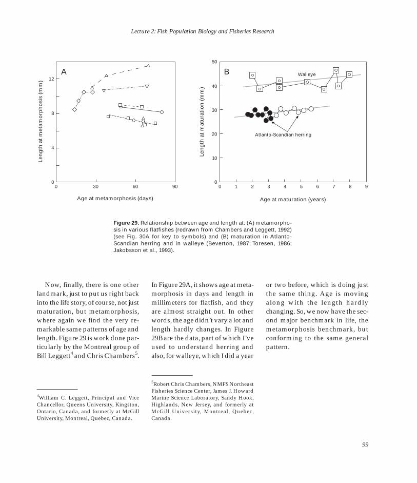
Lecture 2: Fish Population Biology and Fisheries Research Le
ng
th a
t m
etam
orp
ho
sis
(mm
)
Figure 29. Relationship between age and length at: (A) metamorphosis in various flatfishes (redrawn from Chambers and Leggett, 1992) (see Fig. 30A for key to symbols) and (B) maturation in Atlanto-Scandian herring and in walleye (Beverton, 1987; Toresen, 1986;
50
40
30
20
10
0 0
8
12
4
0 30 60 900
A B
Len
gth
at
mat
ura
tio
n (
mm
)Age at metamorphosis (days) Age at maturation (years)
Atlanto-Scandian herring
Walleye
9 8 7 6 5 4 3 2 1
Jakobsson et al., 1993).
Now, finally, there is one other landmark, just to put us right back into the life story, of course, not just maturation, but metamorphosis, where again we find the very remarkable same patterns of age and length. Figure 29 is work done particularly by the Montreal group of Bill Leggett4 and Chris Chambers5.
4William C. Leggett, Principal and Vice Chancellor, Queens University, Kingston, Ontario, Canada, and formerly at McGill University, Montreal, Quebec, Canada.
In Figure 29A, it shows age at metamorphosis in days and length in millimeters for flatfish, and they are almost straight out. In other words, the age didn’t vary a lot and length hardly changes. In Figure 29B are the data, part of which I’ve used to understand herring and also, for walleye, which I did a year
5Robert Chris Chambers, NMFS Northeast Fisheries Science Center, James J. Howard Marine Science Laboratory, Sandy Hook, Highlands, New Jersey, and formerly at McGill University, Montreal, Quebec, Canada.
or two before, which is doing just the same thing. Age is moving along with the length hardly changing. So, we now have the second major benchmark in life, the metamorphosis benchmark, but conforming to the same general pattern.
99

The Raymond J. H. Beverton Lectures at Woods Hole, Massachusetts
25
90
20
60
A. rostratus
P. olivaceus
P. stellatus
P. americanus
R. tapirina
S. solea
A
15
10
30
5
B
T m
T max
Tm *
0 0 0 5 10 15 20 0 1 2 3 4 5 6
Temperature (AC) Temperature (GDD Z 10–3)
Figure 30. Effect of temperature on: (A) age at in this case), and GDD (mean growing degree-metamorphosis in various flatfishes (redrawn days) is an index of ambient temperture derived from Chambers and Leggett, 1992) and (B) age by Colby and Nepszy (1981) as the sum of the at maturation and longevity in walleye (redrawn products of days � degrees >5ºC, this being the from Beverton, 1987). In B, Tm * is the lowest minimum temperature in the growing season physiologically possible age at maturity (2 years which allows growth to take place.
Ag
e (d
ays)
Ag
e (y
ears
)
In view of the importance of temperature and the concern about temperature changes in the ocean that we talked about yesterday, or indeed long-term climatic changes, you can see how each of these two benchmarks is influenced by temperature. Figure 30A shows the relationship between age at metamorphosis and temperature from Bill Leggett’s data (Chambers and Leggett, 1992), markedly coming
down and flattening out. Figure 30B is the age at maturation and maximum age or longevity against temperature in the walleye from my own earlier paper (Beverton, 1987). You’ll see the remarkable similarity and the general shape of those two, and the very considerable effect that these temperature differences had on all three: the age at metamorphosis, the age at maturation, and the maximum age.
I hope that, by ending on that note, it might put all this story— you don’t have to worry about what the individual is doing—back into the overall framework of understanding how a population will try to respond to changes imposed on it by man or by nature. Thank you very much.
100
Lecture 2: Fish Population Biology and Fisheries Research
Vaughn Anthony I forgot to tell you we’ll have an
examination now on all this. I’m sure Ray will take some questions if you have some.
Andy Rosenberg My question is about the point
you made about using the life his-tory strategy for estimating natural mortality. The only one I know who has tried that, and successfully, is Ram Myers, although I don’t think very many people have used that method, probably because it’s so difficult to do the computations. Now that was just a comment. The question is, at one point you mentioned the issue of reversibility, and for the cod and herring cases which you went through in detail, it wasn’t clear to me whether you would suppose they would be equally reversible as changes in fishing pressure or abundance occurred. For herring, you probably have some evidence that they are reversible, but for cod, I don’t know if we have that same evidence.
Ray Beverton I don’t think we have yet seen a
cod population start to come back up again. I hope the Barents Sea cod is now doing so. I mean, it certainly is doing so. Maybe within 3– 4 years, we may begin to see them following up the same as herring.
Andy Rosenberg But even if they are doing dif
ferent things, one holding the size at maturation relatively constant (Fig. 21), the other one moving up and down the growth curve (Fig. 22), would you expect them to be essentially reversible?
Ray Beverton I’m not sure that I could say they
wouldn’t be. I’m not sure that it immediately makes me think one is reversible and the other is not. That’s a point I must admit I really haven’t thought that far through. There is such a difference between the patterns in the two cases. It certainly isn’t just a question of whether one or both is equally responsive to the first. The fascinating thing, of course, is what is it that causes a cod to start to turn at age 6, compared with others at age 14? For the herring and the salmon, the answer is yes. Actually, to take it much further back in salmon, John Thorpe at Pitlochery and Neil Metcalfe of Glasgow have shown (Metcalfe and Thorpe, 1992) that it is a distribution of basic metabolic activity right back to the emerging larvae that sets off a whole series of better feeding, higher feeding rates, earlier feeding, using up yolk sacs and getting feeding quickly, establish parentry, and become more aggressive. The whole thing snowballs once they start. This is detectable within a few weeks of emergence. We’re a long way from
explaining why the size composition of salmon is diverse. It could also be, although I don’t accept it, it could be exactly the explanation for herring. But what about cod? They’re not doing that. They appear to all be growing up the same sort of curve, with some variation, but all basically, on maturation, the same. And yet, one bunch starts at age 6 and another won’t mature until they’re age 14. That is a complete mystery to me. I must admit I’ve only really realized this in the past year or so that there is such a difference between species, one of which is certainly explainable on the classic salmon story, when per-haps Clupeiformes are not that far removed from the Salmonidae. We wish we knew where the Gadoids are somewhere, but that is only a passing comment and does not ex-plain anything. But it opens up some very interesting possibilities; the reverse question is surely one of them. Are they going to be equally responsive in reverse? I don’t know, but we may find out in a short time after cod can get back up again. Thanks for the question.
Vaughn Anthony Some of this is related to where
these fish are caught and where the salmon run. Georges Bank herring for years, for example, never had poor recruitment until age 6 or 7, although full maturity was around age 4. I think some of them didn’t
101

The Raymond J. H. Beverton Lectures at Woods Hole, Massachusetts
go there to spawn, and the sampling was from the spawning grounds in some cases, in some cases not from the spawning grounds. It makes all the difference in the world for the maturity rates.
Hal Caswell If I understood correctly, in de-
scribing the ESS calculations [evolutionary stable strategy], using as your criteria the expected lifetime of the population, one of the properties of lifetime expected reproductive level is insensitive to timing of the reproduction event in the life history. It’s those timing differences that quantities of life, intrinsic rates from the Lotka equation or growth rates. Has anyone looked to see whether the ESS calculations are changed in these cases like using those measures that are sensitive to timing as well as the density average output? The questions involve ages and sizes at maturation. It seems like timing effects might have a role to play here.
Ray Beverton To the extent that the calculation
is done on the change in the aver-age compilation of maturation age, in a sense once you’ve got directly to it, once you specify the K, then you specify the age at which it’s beginning to happen. So there is an age component to that link or the link between maximum reproductive lifetime amount. But, I think you can’t say beyond that value
because you can’t tell what’s happening within it. But on this maturation cohort analysis, that is in-deed casting a setting for some experiment. What is the difference in maximum lifetime biomass production? To some extent, isn’t that your question?
Hal Caswell I don’t think so. I’m asking a dif
ferent question. Suppose you have two different strategies, one of which begins reproducing at 3 years, the other at 6 years, and they both produce the same lifetime re-productive output. Which one is the better strategy? According to the use of lifetime reproductive output as the criteria, they are equal, but according to calculation output, for example (r from Lotka’s equation), they would not be the same. Probably the one which began producing earlier would have the advantage just because of the timing, not because of a change in the amount of the production.
Ray Beverton I think there must be a link be-
tween what I have been showing you happening within one year class and in fact in one population that would get back the rate of in-crease. I haven’t bothered with that at all. It’s totally different timing, and with what I have associated, really different within the measure, different components. What is within that limited framework?
What is the best thing to do? What if the relationship between that were fed back into this population? That has to be a second-stage question. That brings us back to the stock-recruitment story of mine. Bringing in this sort of thing means we have to perhaps ask this, we need a population model which is based on maturation cohorts taken separately. Operating the rules along the line that I’ve been showing and then putting them together each year, now they are all spawning. Now that will develop the next year class which will then split it-self up and maybe, in that way, we can build together the question you were asking. This brings us back to a natural rate of increase alongside the within-life pattern. It’s very unclear what to do with this mess. We’re beginning to develop population models to do this, just beginning to sketch them out. They’re complicated, but that’s how to do it.
Ione von Herbig I understand populations are
limited by the number of spawning females. Do you know of any work or have you noticed any change in sex ratios as a result of fishing pressure over time? I think this might be appropriate to look at.
Ray Beverton Yes, there are changes in the sex
ratio, but not systematically, not in
102

Lecture 2: Fish Population Biology and Fisheries Research
the same way in all species. In the herring, the sexual dimorphism difference is generally very slight. There is, of course, the mature fishing phase, but everything else about them, we don’t really know. Maybe Vaughn can comment on this, but there is very little difference in this. There is more in cod, but not all that much, but it is possible—I expect we have the data, we’ve subdivided it again in half—to do it in two sections. But when you get to the flatfish, that’s very strong. Indeed, remember those two sets of data showing a difference between sexes? Because the natural mortality of males is significantly greater, and lifespan less, the effect of fishing on them is different. In addition, the behavior of males, especially at spawning time, makes them more vulnerable to capture, significantly more so. They are very active; females are quiescent on the seabed. Fishing at that time captures markedly more males than females. So the answer is yes. The real question is whether the greater fishing on males than females is a factor in influencing the reproductive capacity of the population. I don’t think you were really asking that, but my impression is that it’s unlikely that there’s such a shortage of males in most species to really put that at risk. I can only say that in a rather hunchy sort of way without really figuring it out carefully. But I think in most of the species, certainly in the ones
we’ve looked at, I don’t think the shortage of males due to differential fishing is enough to put at risk their reproductive potential.
Vaughn Anthony We can see this in Atlantic
salmon where if you have poor food supply in winter—December, January, and February—they will mature as grilse and come home after one sea-winter, and those grilse are males. But females won’t fall for that, and they’ll stay out a little bit longer. As a result, the two-sea-winter population will be heavy in females and, of course, the one-sea-winters in males. That’s dramatic when you see that.
Ione von Herbig I have seen a lot of variation in
cod on the Scotian Shelf. We catch an awful lot of males which are running ripe and very, very small—27 cm. Along with the large amount of males we caught, only two or three are females. Most of them are behind males in maturation, and there are noticeably much fewer females than males, almost like an aggregation for spawning. I was wondering if fishing pressure had affected them?
Ray Beverton Certainly, in the case of the re
sponse of whales and their response to males and females, but in age and size it’s more marked in males than in females.
Vaughn Anthony Spiny dogfish will school by sex
and size, and you will get a differential mortality rate fishing on the larger females. You will get a disproportionate result of the population of males. More males will be left behind because of the disproportionate fishing mortality rate, so you can get an effect from fishing directly caused by this.
We have to terminate this. I am really pleased with the subjects talked about yesterday (stock-recruitment) and today (growth and maturation). You couldn’t have picked two better subjects for our needs. I’m very happy about that. Thank you very much.
103

The Raymond J. H. Beverton Lectures at Woods Hole, Massachusetts
Literature Cited
Alm, G. 1959. Connection between maturity, size and age in fishes. Rep. Inst. Freshw. Res., Drottningholm, 40:5–145.
Atkinson, G. T. 1908. Notes on a fishing voyage to the Barents Sea in Au-gust, 1907. J. Mar. Biol. Assoc. N.S. 8(2):71–99.
Beacham, T. D. 1983. Variability in median size and age at sexual maturity of Atlantic cod, Gadus morhua, on the Scotian Shelf in the northwest Atlantic Ocean. Fish. Bull. 81:303–321.
Beverton, R. J. H. 1987. Longevity in fish: some ecological and evolutionary considerations. In A. D. Woodhead and K. H. Thompson (Editors), Evolution of longevity in animals: a comparative approach, p. 161–186. Plenum Press, N.Y., 354 p.
————. 1992. Patterns of reproductive strategy parameters in some marine teleost fishes. J. Fish Biol. 41(Suppl. B):137–160.
————, and S. J. Holt. 1957. On the dynamics of exploited fish populations. Fish. Invest., Lond., Ser. 2, 19, 533 p.
————, A. Hylen, and O. J. Østvedt. 1993. Dynamics of maturation in long-lived fish populations. II. Norwegian spring spawning herring. ICES C.M. 1993/H:20, 9 p.
————, ————, and ————. 1994. Growth, maturation, and longevity of maturation cohorts of Northeast Arctic cod. ICES Mar. Sci. Symp. 198:482–501.
Chambers, R. C., and W. C. Leggett. 1992. Possible causes and consequences of variation in age and size at metamorphosis in flatfishes (Pleuronectiformes): an analysis at the individual, population, and species levels. Proc. First Int. Symp. Flatfish Ecol. Pt. 2, Neth. J. Sea Res. 29(1–3):7–24.
Charnov, E. L. 1993. Life history invariants: some explorations of symmetry in evolutionary ecology. Oxford Univ. Press, Oxford, 167 p.
Colby, P. J., and S. J. Nepszy. 1981. Variation among stocks of walleye (Stizostedion vitreum vitreum): management implications. Can. J. Fish. Aquat. Sci. 38:1814–1831.
Cole, L. C. 1954. Some features of random population cycles. J. Wildl. Man-age. 18:2–24.
Comfort, A. 1965. The biology of senescence. Routledge and Paul, London, 257 p.
Devold, F. 1963. The life history of the Atlanto-Scandian herring. Rapp. R.-v. Réun. Cons. Perm. Int. Explor. Mer 154:98–108.
Dragesund, O., J. Hamre, and Ø. Ulltang. 1980. Biology and population dynamics of the Norwegian spring spawning herring. Rapp. P.-v. Réun. Cons. Perm. Int. Explor. Mer 177:43– 71.
Gross, M. R., R. M. Coleman, and R. M. McDowall. 1988. Aquatic productivity and the evolution of diadromous fish migration. Science 239:1291–1293.
Hansen, P. M. 1954. The stock of cod in Greenland waters during the years 1924–52. Rapp. P.-v. Réun. Cons. Perm. Int. Explor. Mer 136:65–71.
Holt, S. J. 1958. The evaluation of fisheries resources by the dynamic analysis of stocks, and notes on the time factors involved. ICNAF Spec. Publ. 1:77– 95.
ICES. 1994. Report of the Atlanto-Scandian Herring and Capelin Working Group, October 1993. ICES C.M. 1994/Assess:6.
Jakobsson, J., and Ó. Halldórsson. 1984. Changes in the biological parameters in the Icelandic summer spawning her-ring. ICES C.M. 1984/H:43, 36 p.
————, A. Guomundsdóttir, and G.o Stefánsson. 1993. Stock-related changes in biological parameters of the Icelandic summer-spawning herring. Fish. Oceanogr. 2(3/4):260–277.
Jónsson, J. 1954. On the Icelandic stock of cod during the years 1928–1953. Rapp. P.-v. Réun. Cons. Perm. Int. Explor. Mer 136:51–57.
Kyle, H. M. 1903. Fishing nets, with special reference to the otter trawl. J. Mar. Biol. Assoc. N.S. 6(4):562–586.
Lambert, T. C. 1984. Larval cohort succession in herring (Clupea harengus) and capelin (Mallotus villosus). Can. J. Fish. Aquat. Sci. 41:1552–1564.
Maynard Smith, J. 1982. Evolution and the theory of games. Cambridge Univ. Press, Cambridge, 224 p.
104

Lecture 2: Fish Population Biology and Fisheries Research
Metcalfe, N. B., and J. E. Thorpe. 1992. Early predictors of life-history events: the link between first feeding date, dominance and seaward migration in Atlantic salmon, Salmo salar L. J. Fish. Biol. 41(Suppl. B):93–99.
Østvedt, O. J. 1964. Growth and maturation of the Norwegian herring. ICES C.M. 1964, No. 141, 9 p.
Roff, D. A. 1984. The evolution of life-history parameters in teleosts. Can. J. Fish. Aquat. Sci. 41:984–1000.
Rollefsen, G. 1954. Observations on the cod and cod fisheries of Lofoten. Rapp. P.-v. Réun. Cons. Perm. Int. Explor. Mer 136:40–47.
Thorpe, J. E. 1989. Developmental variation in salmonid populations. In C. E. Hollingworth and A. R. Margetts (Editors), Fish population biology. The Fisheries Society of the British Isles Symposium, p. 295–303. J. Fish. Biol. 35 (Suppl. A), 363 p.
Toresen, R. 1986. Length and age at maturity of Norwegian spring-spawning herring for the year-classes 1959– 61 and 1973–78. ICES C.M. 1986/H:42, 8 p.
————. 1990. Long-term changes in growth of Norwegian spring-spawning herring. J. Cons. Int. Explor. Mer 47:48– 56.
Williams, G. C. 1957. Pleiotropy, natural selection and the evolution of senescence. Evolution 11:398–411.
105


“Reflections on 100 Years
of Fisheries Research”
LECTURE 3
May 3, 1994
Aquarium Conference Room Northeast Fisheries Science Center


Before I [Steve Murawski] introduce the specific topic that Ray Beverton is going
to speak on and tell you what the house rules are, I would like, if you will oblige me, to make a few personal reflections on Ray Beverton’s career and mine. I certainly wouldn’t put them on the same level, but certainly he has had an influence, as Vaughn Anthony said earlier, on the careers of all of us who work in the field of population dynamics. I first met Ray in the mid 1980’s—I find it difficult to call him Ray—Professor Beverton.
Ray Beverton Please do.
Steve Murawski That certainly illustrates the
type of person he is. I first met him at an ICES meeting in Copenhagen where I had just given a scintillating paper, I’m sure, having to do with something. I can’t even re-member what it was. This guy in the back got up and was really agitated, really excited about some-thing I had said, really enthusiastic. The last thing he said was “And I’d like to get a manuscript for the Journal.” I went to the moderator after the session and said, “Who was that guy?” He replied, “That was Ray Beverton.” I just about died right there, certainly died and went to heaven.
In terms of familiarity with Ray, it goes back farther than that. As most of us who got an education in population dynamics, we had a personal relationship with him be-fore we ever met him, in terms of the books and papers that he has published. Unlike Vaughn’s experience with Richard Van Cleve, who certainly had a reputation, mine was a little less stilted. The first interaction I had with my major
professor talking about Ray’s work is analogous to that shown in Figure 1. It was this miracle part in the middle the professor couldn’t understand, but he said, “It’s in there somewhere.”
Actually it came home to roost after I had completed my PhD work where I thought I had sort of reinvented the world in terms of technological interactions research.
© Sidney Harris
Figure 1. Cartoon drawing, copyright by and courtesy of Sidney Harris (Harris, 1992).
109

The Raymond J. H. Beverton Lectures at Woods Hole, Massachusetts
I got my thesis published and a couple of papers out, and then I started flipping through the last chapter of Ray’s book (Beverton and Holt, 1957) where he had all the economics worked out, the number of shillings per pound, and all the good stuff that I thought I had invented and certainly had to take back in subsequent papers. I am sure that most of our training, either formal or informal, has similar interactions with “Ray the publisher,” and a few of us have been lucky enough to know “Ray the man.”
In terms of today’s talk, the formal title is: “Reflections on 100 Years of Fisheries Research.” I am not sure if that represents your personal history or represents the his-tory of population dynamics or re-search in general. I guess we’ll find out about that. The house rules are going to be these: the first part of his talk is going to be basically his personal reflections, and in the second part we are going to open it up so we can have perhaps a discussion rather than a talk on where we think the next 100 years worth of fisheries research are going. Hopefully we can get some dialogue and interaction with Ray in terms of where he might think we are going and where we might think we are going. With that, I would like to reintroduce Ray Beverton.
Mal
colm
Silv
erm
an, N
MFS
Ray Beverton Thanks Steve. A very fine intro
duction. Thank you very much. I am going to venture to be a little reminiscent on this occasion. I hope that won’t bore you too much, be-cause sometimes it does get dull to hear people talking about them-selves long ago. It’s easy enough to get into a somewhat sort of jaundiced and nostalgic sort of frame of mind. Anyway, I think perhaps there might be a few interesting specifics of one sort or another.
You are quite right. I didn’t re-ally try to go back to 1894, I have to admit, but I did meet a few of the old sages from the pre-Second World War days, in fact pre-First World War days, so I can offer something of a bridge with some people who, to you, would just be names way back in the past.
The way I’ll do it is to just run through the period from roughly the middle of the 1890’s, which is where I think fisheries science, in an accepted sense, came together. There had been, of course, important developments before that through hatchery work in this country as well as in Europe and through the big expeditions, the Challenger expedition, John Murray, and people like that. As we shall see, there had already been beginnings of worries, in the North Sea in particular, about the effects of fishing, which was spreading very rapidly, from the middle of the last century, all into the North Sea. In terms of serious, organized, recognizable fisheries science, as we see it today, it is probably about 100 years ago, of which I came into it on the second part of that time.
110

Lecture 3: Reflections on 100 Years of Fisheries Research
It divides itself quite conveniently and rather quadratically, in a way, into the periods governed by the two World Wars. If we start with the first of those periods, as I just mentioned, several different countries had already begun to realize that they needed to get a better scientific base to work on. In the U.K., we were very much concerned in those days—I say “we”— ”they” were very much concerned in those days with the effects of fishing. E. W. H. Holt (no relation to Sidney, but after whom the post-war research ship Ernest Holt was named) was commissioned by the Marine Biological Association (MBA)—in those days there was no fisheries lab until 1902—to sample the fish on the fish market, on a pontoon at Grimsby, and to establish whether or not the worries of the fishing industry, reporting to several Royal commissions during the latter part of that period about the decline in fish stocks, were genuine or not.
The Scottish people were, in fact, in action even sooner, people like Thomas Wemyss Fulton. I mentioned Harry Kyle this morning; he became the first assessment secretary when ICES started in 1902. In Denmark, of course, the great Christian G. Johannes Petersen, who developed the Petersen tag for flatfish, was concerned with trans-plantation into and out of the Limfjord as an enhancement pro-
gram. So enhancement was very much one of the driving forces in the early days of fisheries science. In Germany, which in those days was a very strong trawling country and had very similar interests to the U.K., there was Friedrich Heincke, who was the turn-of-the-century Director of the Helgoland Biological Station.
Even before the turn of the century, Johannes Reibisch at Kiel, actually had been, I think, the very first to really work out the fact that you could age plaice from the otolith. That was critical, although it wasn’t taken up very seriously for several years. It was well into the 1903–04 period that William Wallace at Lowestoft, in particular, took it further, but Reibisch was the pioneer. Of course, in the Scandinavian countries, the Norwegians had been in action even before this, with Johan Hjort, G. O. Sars, and people like that very much concerned with the fluctuation of their big cod and herring fisheries, and with a strong physical oceanographic backup through people like Martin Knudsen [from Den-mark] and indeed Fridtjof Nansen the explorer, who was very active in those days. It was the realization that all these things ought to be coming together in some way, in-stead of just being done on a national basis, that led to the setting up of ICES in 1902.
I’ll come to that in just a moment, but I think it might be useful if, while I’m staying with the Lowestoft part of it, I tell you just how things did start in those days. As I said, it was the MBA of Ply-mouth which was commissioned to do this survey work by a special Treasury grant, because there was no other base, no other organization to do it. This was where it started, but by the turn of 1900, it was realized that there had to be a more established base.
My very dear friend and colleague, Arthur Lee, who died last Christmas [1993] and was Director in the 1970’s at Lowestoft, a con-temporary of mine in the post-war years with whom I spent many long months up in the Arctic Ocean, fortunately finished and published a wonderful history of the Lowestoft Lab right back to even its precursor days (Lee, 1992). There is some fascinating material in that, and those who are students of history will find it interesting. I expect Tim Smith has made sure he’s got quite a lot of that built into those aspects of his book (Smith, 1994), which I’m very much looking forward to seeing. I am, in no sense, trying to cover that sort of ground in a way that he will be doing. These are just the odd snip-pet or two of things.
111

The Raymond J. H. Beverton Lectures at Woods Hole, Massachusetts
Cen
tre
for
En
viro
nm
ent,
Fis
her
ies,
an
d A
qu
acu
ltu
re S
cien
ce, L
ow
esto
ft, U
.K.
Figure 2. The staff at Lowestoft in 1907. Front row (l–r): W. Wallace, W. Garstang, J. O. Borley. Middle row: L. H. James, A. E. Hefford, Rosa M. Lee, R. A.Todd, G.T. Atkinson, Dykes. Back row: Potter, Arrowsmith, Walton, Ansell.
The first recognized picture very considerable figure, the most First World War. That’s William we’ve got of the Lowestoft staff is leading fisheries scientist in those Wallace [front row, left] who pioin 1907 (Fig. 2) That’s the then-Di- days in the U.K. With him is J. O. neered the work on plaice and rector, Walter Garstang [front row, Borley [front row, right], who be- whose work Adriaan Rijnsdorp middle]. Walter Garstang was a came the Deputy Director after the and I are using to try and recover
112

Lecture 3: Reflections on 100 Years of Fisheries Research
Cen
tre
for
En
viro
nm
ent,
Fis
her
ies,
an
d A
qu
acu
ltu
re S
cien
ce, L
ow
esto
ft, U
.K.
Figure 3. Deck of the RV Huxley and the crew with a catch of, primarily, flatfish.
the early history of it. That’s Rosa Lee [middle row, middle position] of “Lee’s phenomenon” fame— back-calculation of growth rates. That’s George Atkinson [middle row, second from right] as a young man who went off to the Arctic, as I told you this morning, to work on Barents Sea plaice. He was fisheries inspector at Lowestoft until the outbreak of the Second World War when the Lab closed and every-
body went off to the war. He was asked to stay on, and he did after the war, and I remember him for a number of years. He was retired by then, but he lived next door to the Lab and was always in and out the whole time. He was a wonderful man, one of the people who nearly knew how to get on with everyone, whomever they were. George was respected, his advice sought, and his knowledge was enormous. The
others are lesser-known people, but those are the four whose names survive in terms of folklore as well as in publications, Garstang in particular.
The first ship we had was called the Huxley (Fig. 3). It did its first station in November 1902 south-west of Dogger, and there are log-books recorded and surviving from that. That’s a rather dim picture of
113
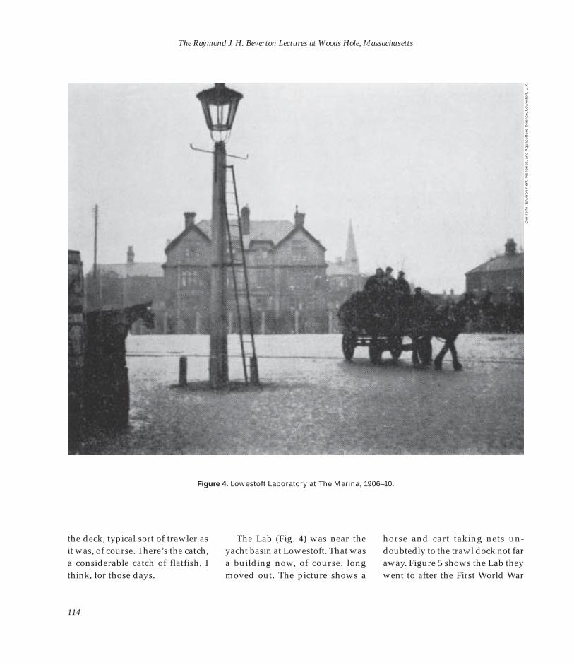
The Raymond J. H. Beverton Lectures at Woods Hole, Massachusetts
Cen
tre
for
En
viro
nm
ent,
Fis
her
ies,
an
d A
qu
acu
ltu
re S
cien
ce, L
ow
esto
ft, U
.K.
Figure 4. Lowestoft Laboratory at The Marina, 1906–10.
the deck, typical sort of trawler as The Lab (Fig. 4) was near the horse and cart taking nets unit was, of course. There’s the catch, yacht basin at Lowestoft. That was doubtedly to the trawl dock not far a considerable catch of flatfish, I a building now, of course, long away. Figure 5 shows the Lab they think, for those days. moved out. The picture shows a went to after the First World War
114

Lecture 3: Reflections on 100 Years of Fisheries Research
Cen
tre
for
En
viro
nm
ent,
Fis
her
ies,
an
d A
qu
acu
ltu
re S
cien
ce, L
ow
esto
ft, U
.K.
Figure 5. The Blenheim and Apsley Houses on the sea front housed the Lowestoft Laboratory during 1920–55.
in which, indeed, I worked at in the Lowestoft, a very imposing build- got to sea and saw the symmetry first few years when we were at ing, seen especially along with its of it, you couldn’t appreciate that Lowestoft, in fact, until 1955. On whole terrace along here, built to it was really a lot more than it the front, on the esplanade at be seen from the sea, and until you might look in that picture.
115
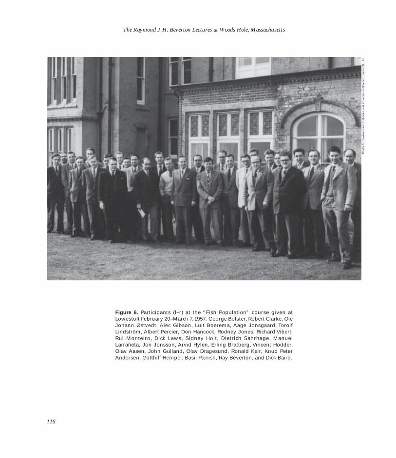
The Raymond J. H. Beverton Lectures at Woods Hole, Massachusetts
Cen
tre
for
En
viro
nm
ent,
Fis
her
ies,
an
d A
qu
acu
ltu
re S
cien
ce, L
ow
esto
ft, U
.K.
Figure 6. Participants (l–r) at the “Fish Population” course given at Lowestoft February 20–March 7, 1957: George Bolster, Robert Clarke, Ole Johann Østvedt, Alec Gibson, Luit Boerema, Aage Jonsgaard, Torolf Lindström, Albert Percier, Don Hancock, Rodney Jones, Richard Vibert, Rui Monteiro, Dick Laws, Sidney Holt, Dietrich Sahrhage, Manuel Larrañeta, Jón Jónsson, Arvid Hylen, Erling Bratberg, Vincent Hodder, Olav Aasen, John Gulland, Olav Dragesund, Ronald Keir, Knud Peter Andersen, Gotthilf Hempel, Basil Parrish, Ray Beverton, and Dick Baird.
116

Lecture 3: Reflections on 100 Years of Fisheries Research
Figure 6 contains a group of people that you probably know some of the names of. In the 1950’s, after I had come to Beaufort, N.C., and done the 1951 course, it was decided, it was really ICES helping to encourage this, that we should run one or two residential population courses at Lowestoft lasting a couple of weeks. This was the second one. There are a lot of people here who subsequently became well known. There was John Gulland, Basil Parrish, Gotthilf Hempel, K. P. “Jydefar” Andersen, there’s me in the corner, Sidney Holt, and so forth. Those courses that we ran, two of them, Basil and Rodney Jones from Aberdeen and Sidney came over to help us do it. It provided a linkage, a knowledge of one another, of methods, as well as people, and stood us in enormously good stead in the later years when the ICES working groups had to really be put together and function. The contacts that we’ve made like this proved to be enormously important.
Lastly, and there’s a certain poignancy in giving you a history of this, because Figure 7 is the Lowestoft Lab as it is now. We moved to the Grand Hotel, as it was called, in 1955, which is that part of the building [in the center]. I was there for 10 years until 1965. We didn’t have any of the building [right side] at the time. It was built much later to house radio-
Figure 7. The Fisheries Laboratory, Lowestoft, in 1982.
Cen
tre
for
En
viro
nm
ent,
Fis
her
ies,
an
d A
qu
acu
ltu
re S
cien
ce, L
ow
esto
ft, U
.K.
biology, which was previously down on the docks. A lot of the buildings along this [far left] end and behind, that you can’t see, have been added since then for experimental facilities. This is a lovely position on the sea front, with the beach and bathing huts and so forth, because I think there are changes afoot now of which we have never seen the light for the
whole of the times. It is very likely that Lowestoft and Aberdeen are going to be put under single management. This is only hearsay at the moment; I haven’t really heard it very positively, but Emory knows a bit about it. It looks as if it will, not surprisingly, with the Lowestoft fishing industry now one-fifth the size of the Scottish.
117
The Raymond J. H. Beverton Lectures at Woods Hole, Massachusetts
118

Lecture 3: Reflections on 100 Years of Fisheries Research
Once the distant-water fishing was gone in the 1970’s, with the extension of 200-mile limits, that changed totally the relative balance of the commercial interest in fishing in England compared to Scot-land. Prior to that, it was 2 or 3 to 1 the other way. Since then, the Lowestoft and Grimsby fishing has itself subsided. Lowestoft made, I think, a complete hash of picking up threads again. In the meantime, the Dutch went steaming ahead with their beam trawls, advanced beam trawl technology, and left Lowestoft far behind. That withered even further, and as a result the imbalance is so strong that the cries, which have been heard all through the century for some form of amalgamation between the two labs, Aberdeen and Lowestoft, have now become, I think, turned into reality of some form. I don’t think that means the Lab will disappear. It just means that the position will be probably, as you like, like a substation to Aberdeen. It’s not surprising that sort of thing will happen because the new factor that’s come into it is Brussels and the European Community (E.C.). There is a considerable possibility, and some logic behind it,
Figure 8 (opposite page).Text of a letter exchanged between two officials of H.M. Treasury in December 1909 regarding fisheries research in the United Kingdom. (Provided by John Ramster, former oceanographer at the Lowestoft Laboratory.)
CW
T/y
ear
1,000
800
600
400
200
0 1860 1870 1880 1890
Haddock
Plaice
Year
Figure 9. CPUE (hundredweight/year) of had-dock and plaice recorded by four Grimsby sailing trawlers, 1867–90 (redrawn from Garstang, 1900) (CWT = 100 lb.).
that Brussels will become the funding source for the assessment work for the E.C. fisheries, which includes the North Sea; funded to strong countries and then refunded back on a contract basis to different groups, rather than different countries, to do different things.
I’d just like to leave this early period with a lovely minute (Fig. 8) between two Treasury officials which Arthur Lee unearthed and John Ramster put in our newsletter a year ago, because it was a great argument as to who should be paying for this. The MBA would be funded directly from the Treasury grant, but the Treasury didn’t want to get involved in arguments
going on even then between Aberdeen and Lowestoft as to who should do what. So there is a lovely minute from one Treasury official to another with a stinger at the end of it all which you might find interesting. I have a facsimile of the original in very nice handwriting.
Right, so let’s leave the history of the Lab, as far as the Lab itself is concerned. I’ll come now to the more scientific work and bring in the part of it that I had more to do with in the post-war years. Garstang had charge of this early investigation into what was happening with North Sea plaice fisheries over the latter part of the last century (Fig. 9). The paper he wrote in 1900 was
119
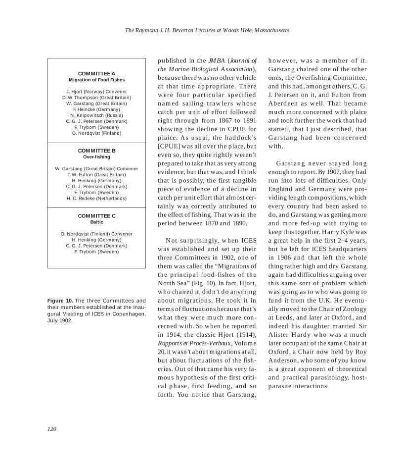
The Raymond J. H. Beverton Lectures at Woods Hole, Massachusetts
COMMITTEE A Migration of Food Fishes
J. Hjort (Norway) Convener D. W. Thompson (Great Britain)
W. Garstang (Great Britain) F. Heincke (Germany)
N. Knipowitsch (Russia) C. G. J. Petersen (Denmark)
F. Trybom (Sweden) O. Nordqvist (Finland)
COMMITTEE B Over-fishing
W. Garstang (Great Britain) Convener T. W. Fulton (Great Britain)
H. Henking (Germany) C. G. J. Petersen (Denmark)
F. Trybom (Sweden) H. C. Redeke (Netherlands)
COMMITTEE C Baltic
O. Nordqvist (Finland) Convener H. Henking (Germany)
C. G. J. Petersen (Denmark) F. Trybom (Sweden)
Figure 10. The three Committees and their members established at the Inaugural Meeting of ICES in Copenhagen, July 1902.
published in the JMBA (Journal of the Marine Biological Association), because there was no other vehicle at that time appropriate. There were four particular specified named sailing trawlers whose catch per unit of effort followed right through from 1867 to 1891 showing the decline in CPUE for plaice. As usual, the haddock’s [CPUE] was all over the place, but even so, they quite rightly weren’t prepared to take that as very strong evidence, but that was, and I think that is possibly, the first tangible piece of evidence of a decline in catch per unit effort that almost certainly was correctly attributed to the effect of fishing. That was in the period between 1870 and 1890.
Not surprisingly, when ICES was established and set up their three Committees in 1902, one of them was called the “Migrations of the principal food-fishes of the North Sea” (Fig. 10). In fact, Hjort, who chaired it, didn’t do anything about migrations. He took it in terms of fluctuations because that’s what they were much more concerned with. So when he reported in 1914, the classic Hjort (1914), Rapports et Procès-Verbaux, Volume 20, it wasn’t about migrations at all, but about fluctuations of the fisheries. Out of that came his very famous hypothesis of the first critical phase, first feeding, and so forth. You notice that Garstang,
however, was a member of it. Garstang chaired one of the other ones, the Overfishing Committee, and this had, amongst others, C. G. J. Petersen on it, and Fulton from Aberdeen as well. That became much more concerned with plaice and took further the work that had started, that I just described, that Garstang had been concerned with.
Garstang never stayed long enough to report. By 1907, they had run into lots of difficulties. Only England and Germany were providing length compositions, which every country had been asked to do, and Garstang was getting more and more fed-up with trying to keep this together. Harry Kyle was a great help in the first 2–4 years, but he left for ICES headquarters in 1906 and that left the whole thing rather high and dry. Garstang again had difficulties arguing over this same sort of problem which was going as to who was going to fund it from the U.K. He eventually moved to the Chair of Zoology at Leeds, and later at Oxford, and indeed his daughter married Sir Alister Hardy who was a much later occupant of the same Chair at Oxford, a Chair now held by Roy Anderson, who some of you know is a great exponent of theoretical and practical parasitology, host-parasite interactions.
120

Lecture 3: Reflections on 100 Years of Fisheries Research
One of the little gems of those early days, which isn’t widely known, and in fact I hadn’t spotted it until, a couple of years ago, Emory asked me to do a little piece for the ICES newsletter. I had been reading the Heincke report, which was 1913, on all this plaice story be-cause of the study that I’m doing now with Adriaan Rijnsdorp of IJmuiden trying to reconstruct some of this early dynamics. I was struck by the fact that he had spotted, or appeared to have spotted, that they could plot the logs of the length compositions and get a very nearly, on the right-hand side, straight line. He had said that means that log N is A + B × L, and if that’s a general rule—which he said he did not believe—then it means we have a means of constructing a life table. In fact, it wasn’t Heincke, it was Thomas Edser, who was the statistician in London assigned to the organization of the massive 5 million length compositions that came in over those first 2–3 years in Lowestoft, 1905–07. He wrote in a paper in the Journal of the Royal Statistical Society in 1908 which, in fact, had that in it, as you will see (Fig. 11) on the first page where he says that “It appears that, within certain limits, the number of plaice at any length is directly related to that length by a formula of the type, log Figure 11. Reprinted first page from Edser (1908) from the Jour
y = A + bx where y is …” etc., etc. nal of the Royal Statistical Society regarding commercial
He produced the length com- length samples of plaice from the southern North Sea.
position and logged the whole of
121

The Raymond J. H. Beverton Lectures at Woods Hole, Massachusetts
Loga
rith
m o
f th
e n
um
ber
of
pla
ice
4
3
2
1
0
10 20 30 40 50 60 70
Length of plaice in centimetres
Figure 12. Reprinted plot from Edser (1908) of the logarithm of numbers vs. length for plaice taken from the southern North Sea in 1906.
5 it (Fig. 12). So there’s a nice little piece of population demography dating back to 1906. Actually, to be fair to Heincke, he did sort of put that reference to Edser, and I don’t want to be trapped for a moment on the very great achievement that Heincke had in the whole exercise. He took over this exercise from Garstang and knocked it into shape, got help with the analysis of the data, and really produced the first assessment working group report with a recommendation that the size limit should be increased from almost nothing—they were catching an average size of around 17–18 cm—up to 21 or 22 cm. That sounds pretty modest for today, but still it didn’t come into effect, because the First World War stopped it. It probably wouldn’t have come anyway because there was no kind of official arrangement for this. It was just ICES writing around to member governments. The Belgians, amongst others, were already beginning to say “We’re not having anything to do with this. This will upset and wreck our fishery.” So, in fact, it never came into force.
Moving into the post-First World War period, of course, that starts with one of the great contributions Fiodor Ilyich Baranov published in 1918, in Russian of course (Fig. 13). We didn’t see it in the Western world until the latter part of the 1930’s. I didn’t see it until 1947, but
122

Lecture 3: Reflections on 100 Years of Fisheries Research
it had been seen. E. S. Russell, who was then Director of Lowestoft, had picked it up. This particular translation was, in fact, published by our Foreign Office and copied through to the California State Fisheries Laboratory by the Inter-national Fisheries Commission in 1943. That’s the equation at the bottom. All you need to know is that it is a length-based yield biomass equation with a linear growth function (RwL3 q), and indeed it is exactly that with that formulation in it.
In the post-war period, Baranov wasn’t known. His paper didn’t have any effect at all because it disappeared into the limbo with the First World War and the Russian Revolution. He was an engineer, not a biologist, and was put onto other things and rather disappeared, certainly from Western view. I have never heard or seen him, and I’ve never heard of any-one else who met him, except for one or two Russians whom I’ve met from time to time.
During the inter-war period, of course, was when the sigmoid curve first appeared, and the birth, by Raymond Pearl originally in this country from the point of view of human demography, of the idea of the logistic growth (Pearl, 1925). It was the Norwegians—Per Ottestad—from the point of view of whaling (Ottestad, 1933), who
Figure 13. Reprinted portions of the classic paper by Baranov (1918).
123

The Raymond J. H. Beverton Lectures at Woods Hole, Massachusetts
Cen
tre
for
En
viro
nm
ent,
Fis
her
ies,
an
d A
qu
acu
ltu
re S
cien
ce, L
ow
esto
ft, U
.K. first realized this could possibly be
the basis for population and yield assessment. Michael Graham, who was my Director after the war; here he is as a younger man (Fig. 14); his main species was cod—that’s in the 1930’s, realized that this was a potential way of coping with the problem of assessment, and he rather cleverly used changes in abundance during the First World War to try to get some estimate of the natural rate of increase and used it to develop the idea of getting a maximum yield (Fig. 15). In fact, it was more luck than any-thing else, but he didn’t get it far wrong back at that time. He didn’t put formal mathematics into it, but left it essentially in that sort of form [as in Fig. 15]. It wasn’t until 1954 when Benny Schaefer picked it up and really did it systematically (Schaefer, 1954). Before that, Ottestad was probably the first to do that exercise.
Figure 14. Michael Graham, Director of the Lowestoft Laboratory, 1945–58, marking a cod aboard ship.
124
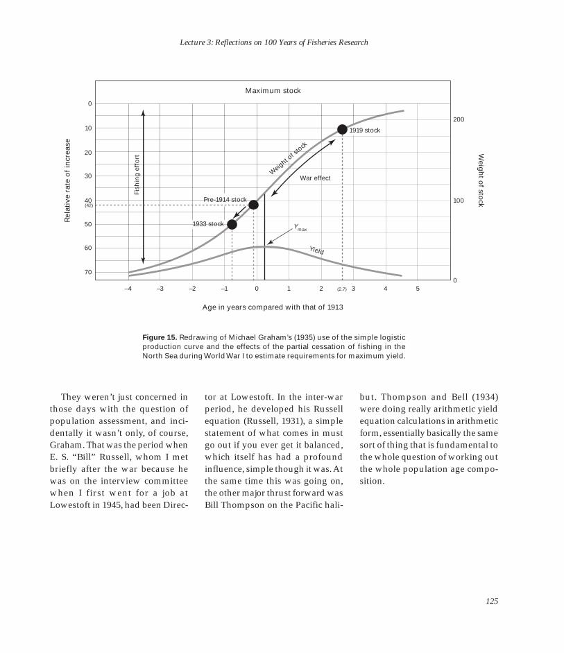
Lecture 3: Reflections on 100 Years of Fisheries Research
0
Rel
ativ
e ra
te o
f in
crea
se
20
Figure 15. Redrawing of Michael Graham’s (1935) use of the simple logistic production curve and the effects of the partial cessation of fishing in the North Sea during World War I to estimate requirements for maximum yield.
Maximum stock
10
30
40
70
–4 –3 –2 –1 0
200
100
Age in years compared with that of 1913
(2.7)
Y max
War effectW
eight of s
tock
0
Fish
ing
eff
ort
Pre-1914 stock
1933 stock
1919 stock
Yield
5 4 3 2 1
(42)
Weig
ht o
f stock
50
60
They weren’t just concerned in those days with the question of population assessment, and incidentally it wasn’t only, of course, Graham. That was the period when E. S. “Bill” Russell, whom I met briefly after the war because he was on the interview committee when I first went for a job at Lowestoft in 1945, had been Direc
tor at Lowestoft. In the inter-war period, he developed his Russell equation (Russell, 1931), a simple statement of what comes in must go out if you ever get it balanced, which itself has had a profound influence, simple though it was. At the same time this was going on, the other major thrust forward was Bill Thompson on the Pacific hali
but. Thompson and Bell (1934) were doing really arithmetic yield equation calculations in arithmetic form, essentially basically the same sort of thing that is fundamental to the whole question of working out the whole population age composition.
125
The Raymond J. H. Beverton Lectures at Woods Hole, Massachusetts
Simplified view of brood years, classified.
1904 =
=
=
=
= Figure 16. Cod year-class
= strengths (redrawn from
=Sund, 1936). =
=
=
1917
=
=
=
1922
Stock
1897
1900
1910
1920
1930
8
9
3
4
05
6
7
8
9
1
2
3
4
5
6
7
8
9
1
2
3
4
5
6
7
8
9
1
2
3
4
35
1
2
Area Gr Ic Br Fi Lo Fa Sk Da NS Bl
N-W A-N L L L L L
Gr
Ic
N-W
A-N
L
Br
Fi
Lo
Fa
Sk
Da
NS
Bl
1) 1) 1) 1) 1)
=
=
=
=
=
1) Based on 2 samples from the West Coast (Lat. 59° and 62° N).
Areas thus:
West Greenland
Iceland
Barents Sea
Finnmark coast
Lofoten
Faroe
Skagerrak
Danish waters
North Sea
Middle Baltic
Symbols
very rich
rich
medium
lean
very lean
Stocks thus:
Iceland-Greenland
Arcto-Norwegian
Local
126
Lecture 3: Reflections on 100 Years of Fisheries Research
Jahrgang
Island: West Nord Ost Süd
Nördl. Nordsee: Moray Firth Aberdeen- u. Lunan- B Carnoustie- u. St. Andrews- B Firth of Forth
Südl. Nordsee:
1923
19
24
1925
19
26
1927
19
28
1929
19
30
1931
19
32
1933
19
34
1935
1918
1914
19
15
1916
19
17
1919
19
20
1921
19
22Ostfries. Küste Holländ. Küste
Nordfries. Küste Hornsriff-Gebiet Limfjord (Nissum)
Gesamt (Engl. Dampftrawler)
Übergangsarea: Skagerrak
Dän. K.:
Dän. K.: Schw. K.:
Schw. K.:
Nördl. Kattg
Südl. Kattg Beltsee
Westl. Ostsee
Ostsee
{ {
A
............................................. ............................................
............................................... ..............................................
................................. ...............
... ...............................
....................................
..........
..............................
.............................................
............
............................
............................ ......................... .........................
......................
...
But it wasn’t just that sort of thing. There were very interesting ICES-sponsored symposia. They were just the same sort of things we have now on, for example, year-class strength. In the 1936 Rapports, they were looking at year-class strengths coming through from sampling on a number of species. In this case (Fig. 16), it was cod which Oscar Sund, a Norwegian cod expert, put together, and they were able to pick out a synchrony of good year classes—1904, 1917, 1922 in the same volume and using the same symbols, so it was obviously an organized exercise. Adolph Bückmann, the German flatfish expert of that period, did the same thing for plaice (Fig. 17A), picking out the 1922 and 1928 year classes. Here is the haddock (Fig.
Icel
and
Faro
e
Ro
ckal
l
W. S
cotl
and
N
. Ire
lan
d
No
rth
Sea
Ska
ger
rak
Kat
tega
t B
elt
Sea
W
. Bal
tic
No
rway
Bea
r Is
lan
d
Bar
ents
Sea
17B), rather less clear-cut, but still evident. This was Robert Clark, who was then Director of the Aberdeen Lab, picking out the strong
Year-B Class
1916 1917 1918 1919 1920 1921 1922 1923 1924 1925 1926 1927 1928 1929 1930 1931 1932 1933 1934 1935
Figure 17. Plaice (A) year-class strengths (redrawn from Bückmann, 1936) and
Comparison of age groups in different regions haddock (B) year-class strengths (re= Poor = Intermediate = Abundant drawn from Clark, 1936).
127

The Raymond J. H. Beverton Lectures at Woods Hole, Massachusetts
1941
1942
1943
1944
1945
1946
1947
1948
1949
1950
1951
1952
1953
1954
1955
1956
1957
1958
1959
1960
1961
1962
1963
1964
1965
1966
1967
1968
1969
1970
1941
1942
1943
1944
1945
1946
1947
1948
1949
1950
1951
1952
1953
1954
1955
1956
1957
1958
1959
1960
1961
1962
1963
1964
1965
1966
1967
1968
1969
1970
Year
-cla
ss
Geo
rges
Ban
k 5Z
had
do
ck
Bro
wn
s B
ank
4X h
add
ock
B
row
ns
Ban
k 4X
co
d
Geo
rges
Ban
k 5Z
co
d
Sab
le I.
Ban
k 4W
had
do
ck
4W a
nd
4V
s co
d
St.
Pie
rre
Ban
k 3P
s h
add
ock
S
t. P
ierr
e B
ank
3Ps
cod
G
ran
d B
ank
3N +
3O
had
do
ck
Gra
nd
Ban
k 3N
+ 3
O c
od
Ic
elan
d
had
do
ck
Icel
and
co
d
Eas
t G
reen
lan
d
cod
W
est
Gre
enla
nd
co
d
Arc
to-N
orw
egia
n
had
do
ck
Arc
to-N
orw
egia
n
cod
So
uth
ern
Gu
lf S
t.
Law
ren
ce 4
T c
od
No
rth
Sea
h
add
ock
Year
-cla
ss
?
?
?
?
?
?
?
?
?
?
+
+
+
+
+
+
+
+
+ ?
?
Figure 18. Successful year classes of cod and haddock in various areas of the North Atlantic (Templeman, 1972).
128

Lecture 3: Reflections on 100 Years of Fisheries Research
year classes there. It wasn’t, of course, until Wilf Templeman (1972) picked this up again in 1972 in an ICNAF publication (Fig. 18) and traced the synchrony again across the whole of the North Atlantic cod stocks. I don’t think he had realized that sort of approach had been done earlier. As far as I can tell, he didn’t, but there you are, it’s the same parallel thinking again.
I did my first two years at Cam-bridge in 1940–42 and then—I was initially going to be a chemist, and did physics, maths, chemistry, and things at school, no biology—when I got back to Cambridge, I had to take a third major subject, and I took zoology. You couldn’t take mathematics as a science subject in those days. You had to do it as an extra half subject. I was playing football [rugby] for the University and needed two afternoons a week for training. Those two afternoons clashed with the 4 o’clock lecture of maths on the half-subject track. I stuck with the maths for a little while until I got to a point halfway through the second term with the Oxford-Cambridge match moving up two weeks ahead. I played left fullback and we had the Oxford captain on the right wing against us and he was very fast and very strong and they said, “You’d better get fit or don’t collapse halfway through the game.” So I was beginning to watch my time allocation.
We got to a lecture by a chap named Todd, who actually had written a textbook on algebra, and he was showing us how to develop the method of solving a cubic equation, for which there are two or three methods. One is by Newton’s method and another by Carlton. Well, he started with Newton’s method and this covered two whole blackboards that size. It got pretty complicated when you are trying to put together all the various terms. Now, at about 4:55 pm, he looked at it and said, “Oh, I’m terribly sorry, but I’ve made some mistake and have to do it over.” So I thought I’d give it one more try. So, the next week he got Newton’s right after about 10 minutes and then he went on to Carlton’s method of doing it, and the same thing happened. At about 5 o’clock he said, “I’m terribly sorry; we’ll have to leave this question. You can look it up in your textbook anyway.” That wasn’t the best use of my time in those days, so I didn’t do maths anymore at Cambridge. I had done enough to get me by, and by the late 1940’s, one or two textbooks were appearing on mathematics and biology, as there was no such thing at first.
Anyway, to cut a long story short, my professor at Cambridge, James Gray, said, “Why don’t you spend a few months at Lowestoft before you come back to do your final year? They’ll have to rebuild,
they have quite a few people, and they need some people with some reasonably quantitative skills. That’s the way it’s going.” So I did, and went in the autumn of 1945 and was immediately taken off to sea by Michael Graham in the Arc-tic on a commercial trawler that had just been decommissioned from the war from mine sweeping—filthy dirty and smelly, covered in rust and everything. He had said, “We have to have an Arc-tic program after the war and we’ll have to have a research vessel if we want to find out what’s going on.” I went on that trip, but wrote up my resignation three times. We steamed straight out in a gale in the North Sea and I was in the fo’c’sle with a smokey coal fire going, and there were some good old chaps up there. Oh dear, it was a time! How-ever, it was never as bad again, and I didn’t submit my resignation. When I finished my last year, I knew this was what I wanted to do.
In that first period before I went back, in the spring of 1946, Sidney Holt came. He had just finished at Reading University where Basil Parrish 4 years previously had graduated. Michael Graham said, “I want the two of you to really see if you can’t put the whole of this fish population stuff on a more substantial basis. We’ve had a go at it, the sigmoid curve stuff. Thompson is doing arithmetic over in Seattle, and it really needs a
129

The Raymond J. H. Beverton Lectures at Woods Hole, Massachusetts
Figure 19. Reprint of “Population Studies in Fisheries Biology” by Hulme et al. (1947).
more systematic approach.” When your own devices. I can’t tell you protect you any longer. You’ll have I came back to the Lab in 1947, I how to do it. I’m satisfied you to take a chance after that, but for remember him saying to the two know more than I can tell you those 4 years, I will.” We did have of us, “Well, I’ll give you 4 years. about it. It’s up to you. If you don’t 4 years together, 1947–51. We were We’ll leave you alone for 4 years to succeed at the end of 4 years, I can’t left to our own devices. We had a
130
Lecture 3: Reflections on 100 Years of Fisheries Research
room for ourselves in an adjacent house next door to the Lab deliberately to put us away from the rest of them, and it was a wonderful time. Sidney and I got on wonder-fully together. We never had an argument or a cross word or any-thing. We just simply found we had that sort of partnership that doesn’t often happen. It was just superb.
Figure 19 shows a little paper by a chap named Henry Hulme, who was in Operational Research with Michael Graham. He was his aide and, in fact, died not long ago (1991). He was a very considerable figure. They were working up the theory of convoys and how to place and do convoy work in relation to the U-boats and so on. Graham said to Hulme, “Come down to the Lab and talk to my two young boys.” And so he did, and out of this came a paper we wrote, which is really what Baranov put in an age-specific form instead of a length-specific one and still with a linear growth rate, and that was in Nature. Some people afterwards said, “What was Hulme, Beverton, and Holt (1947)?” Well, that’s what it was, and it was done while I was still at Cambridge. I was sent the draft and so on. I hadn’t come back to the Lab yet.
When we did come back, Sidney had discovered Bertalanffy (Fig. Figure 20. Reprint of the first page of “Problems
of Organic Growth” by von Bertalanffy (1949).20). This was the summer of 1947.
131

The Raymond J. H. Beverton Lectures at Woods Hole, Massachusetts
Cen
tre
for
En
viro
nm
ent,
Fis
her
ies,
an
d A
qu
acu
ltu
re S
cien
ce, L
ow
esto
ft, U
.K.
Figure 21. Photo of Ray Beverton (left) and Sidney Holt (right) at work on their magnum opus in 1949 in the Fisheries Laboratory, Lowestoft. Ray can be seen working next to a three-dimensional cardboard model of a yield isopleth diagram, while Sidney can be seen operating a hand-Brunsviga calculating machine.
He did so because he had two very good friends at Reading. One was a mathematician, Bill Thomas, who taught him, and me, quite a lot of maths. The other was a physiologist, Peter Jewel, who actually became Professor of Physiology at Cambridge, which is a very prestigious Chair, but he himself more ran the department while people
like Alan Hodgkin and other great names, Nobel Prize winners, did their grant and private work. Peter Jewel picked up Bertalanffy, be-cause Bertalanffy was a human physiologist. He had wide talents, but that was his special field. He introduced this to Sidney, and Sidney immediately realized that this was what we were looking for.
When I came back, he said, “Look, I think I’ve got the equation. Let’s put it into the yield equation.” In no time at all, we were able to do that, and the algebra comes out quite neatly except for a few places. But the original von Bertalanffy (1938, 1949) formula was, of course, unspecified. It didn’t specify what those two powers [n and m] were.
132

Lecture 3: Reflections on 100 Years of Fisheries Research
Pro
f. J
oh
n G
. Sh
eph
erd
, FR
S
Figure 22. Sidney Holt (left) and Ray Beverton (right) at the April 1–6, 1984, Dahlem Workshop in Berlin on Exploitation of Marine Communities.
It was anabolism and catabolism, and we often found the need to go back to that formulation of it in terms of weight, which is what this was, rather than worrying about the length version of it. And so did other people like Andersen and Ursin (1977), when they developed the multispecies version of it, and Jan Beyer and others, who picked up the whole question of length-based methods and tried to build
in and simulate food, growth, and so on. They often found it’s much better to go back to that basic formulation. Even if you put 2/3 and 1 as powers in Bertalanffy’s equation, you are still back into a basic dw/dt formulation.
So, it was really getting the Bertalanffy off the ground that gave us the lead we wanted. And then as long as we knew how to
adjust for density-dependent growth, a whole lot of things came up. Figure 21 shows Sidney and me in 1949 with our yield isopleth— that’s in the frontispiece of the re-print (Beverton and Holt, 1993) of our 1957 book—in this little room of ours in the next-door house beavering away at our work.
Figure 22 is another picture of Sidney and me at the 1984 Dahlem
133
The Raymond J. H. Beverton Lectures at Woods Hole, Massachusetts
Workshop1 where we had one of the discussion groups; Sidney chaired and I was rapporteur. The Lowestoft people, when they saw that, suggested that I was saying, “Come off it, Sidney, you can’t do that.” It probably was their comment too.
By this time, Sidney had achieved a wonderful result. He had saved the great whales in the early 1970’s. He became very much involved with whales, firstly from FAO, and then he gradually lost interest in FAO and became more and more concerned with whales and whaling conservation. By setting up very rigorous standards for any kind of whaling approval, he really took the Japanese, in particular, to the cleaners on this one. They couldn’t match this, and it really meant that they stopped whaling just in time to save the great whales. Of course, it’s gone on rather more than that since then and has become a very much more politicized exercise. So, there’s Sidney, and now if you ever saw him, he’s still got a mass of white hair, beard, and he’s got little dots
1Workshop held in Berlin April 1–6, 1984 on Exploitation of Marine Communities (May, 1984). Dahlem Workshops were be-gun in 1974 to promote an interdisciplinary exchange of scientific ideas and to stimulate cooperation in research among inter-national scientists. These workshops involve invited experts who engage in concentrated discussion on specific topics.
up there, and he’s just one mass and looks like a real guru!
I think I’ve gone on for so long I’m not going to spend more than just a few minutes picking up a few of what I think are the highlights since then and then I’ll hand over to Steve.
I suppose going into the 1950’s and the 1960’s—let me just consult my little aide-memoire—we had finished really all our work on the book by 1951 or 1952. Sidney wasn’t happy; he didn’t like sea-going, and he didn’t really like Lowestoft very much as a place. When Geoff Kesteven came over in the early 1950’s headhunting for setting up the Fisheries Division of FAO, he said to Sidney, “Will you come over and start it up with me?” And Sidney did. So from then onwards, I did the writing of it from 1952 to 1954. We kept ex-changing letters and every time Sidney got back to the U.K., which he did quite a few times during the year (his parents were still there), we would have all-night sessions at Lowestoft. We were ever working on new ideas and ways of putting things, and so forth—wonderful times. So by 1954, the manuscript was finished and Michael Graham said, “Right, we’ve got to get it published at the Stationery Office.”2 He took it up there and they wouldn’t have anything to do with it at all. He said, “All right, if
you don’t do it, I’m resigning as from now.” They didn’t believe him, but, of course, he actually was serious, and within a day or two, they had capitulated. They took 3 years to publish it. It wasn’t until 1957 that it finally appeared. They actually did very well. There were very, very few typos, considering the complexity of some of it, which, looking back, was a bit over the top, but still that’s the way it was.
Vaughn Anthony What was their problem with it?
Too long?
Ray Beverton Too big! I mean, how many were
they going to sell? We had great difficulty persuading them to print 1,500 of them, and they thought they’d be lucky to get rid of 100. It was expensive to do, too. It took 3 years to do it because it was so large and with detailed typesetting. There were no modern methods available then.
In the meantime, in 1954, out came Bill Ricker’s classic on stock and recruitment. It was really— you mentioned about chaos, yes we addressed that—an Oxford statistician, Paul Moran, in a paper in 1950 on insects (nothing to do with fish) that he [Ricker] spotted,
2Her Majesty’s Stat. Off., publisher of official U.K. documents.
134

Lecture 3: Reflections on 100 Years of Fisheries Research
who found that if you get a degree of feedback, stronger feedback in a difference equation from one term back to the next, you can get some very funny things. He did, in fact, a stock-recruitment curve with a replacement line on it. I know Bill didn’t know it, and we didn’t know it, but Bill worked this one out. And that classic stock-recruitment paper, when we saw it we thought, “Oh, God, this has driven the coach and horses through it.”
With a sigh of relief, however, we realized that he hadn’t actually tackled it from the way we had at all. He had gone for a totally different formulation, and so the two approaches still survive as the two basic ways of looking at stock and recruitment. Incidentally, it’s all a question of time lag. In the Beverton and Holt equation, which is a dN/dt view on N – µ2N
2, it’s instantaneous. The density at that moment determines the mortality rate, but in Ricker’s equation, the density-dependent part is back-dated to the initial numbers, N0. Contemporary abundance has no effect at all. It’s entirely based on the original starting numbers, or the adult population, if you turn the original numbers back to the previous parents. So those are the extremes of no time-lagging and complete time-lagging. If you are interested in thinking in terms of a relationship between them, that’s one way of looking at it.
Moving on briefly to the 1960’s, heimo and Dickie (1964) on catch-I think that, by then, one of the big ability, and several others—a clasdiscoveries in the 1960’s was VPA3. sic Rapports. Every now and again, Normally regarded as developed the Rapports really hit the right by John Gulland (1965) in an ap- moment when everything came pendix to an ICES Arctic Fisheries together. There were a number of Working Group report, in fact it others where this was done, e.g., was discovered before and simul- “Fish Stocks and Recruitment” at taneously by Garth Murphy, in- Aarhus in 1970 (Parrish, 1973), cidentally from California (Murphy, “The Biological Basis of Pelagic 1965). I’m sure they had no kind of Fish Stock Management” in Aberknowledge of each other’s efforts, deen in 1978 (Saville, 1980), and but it was the idea of back-calcu- “Early Life History of Fish” here in lating instead of forward-calculat- Woods Hole in 1979 (Lasker and ing that was obviously dawning on Sherman, 1981). several people at once over that time. I think, of course, the beginnings
of the dimension of this story, The earliest record I’ve found of which we have begun to get in-
it was Rodney Jones (1961), in an volved in, really dropped out once appendix again. It’s a very reluc- the discrete time business came on tant discovery; it always appeared the street, because you didn’t want in an appendix with something to worry about the yield equations else. This was an appendix to a or the purely equilibria. Once you paper he did in 1961 on calculation do it on a year-to-year basis, you of mesh increase. He said, “Look, have your weight-at-age table and if you work this backwards, this don’t bother about growth rates catch equation business, lo and be- and things as such, but I think per-hold, it doesn’t matter what F you haps we are beginning to have to start with, it will converge.” He left think a bit more about them now. this as an appendix and then brought it into a paper at the 1963 However, then, of course, ICNAF ICES Symposium on “The Mea- was well on stream. I had some surement of Abundance of Fish wonderful times with ICNAF and Stocks,” which I think was again its Assessments Subcommittee and one of the landmarks because it not with ICES all at the same time. By only included Rodney’s paper the late 1960’s and early 1970’s, the (Jones, 1964), but it included Palo- collapses that I talked about yes
terday began to influence a lot ofthe way fisheries science was mov-
3Virtual population analysis. ing. The daily [otolith] rings were
135

The Raymond J. H. Beverton Lectures at Woods Hole, Massachusetts
discovered in 1974, and by then the computer was coming on stream. Now that was somewhat of an animal that we never had anything to do with at all. All our calculations had to be done by hand-Brunsviga4, so you can imagine when we did our density-dependent stock and recruitment and growth rate [and] put [it] into our haddock thing, which was probably the pinnacle of our modeling efforts. It took about 8 months to get that done. The only way we could solve these four simultaneous equations, growth and every-thing, was by taking batteries of things and plotting until you got the answers.
So, the VPA didn’t come easily. It caused quite a lot of “cububble“ until people really realized just how complicated it was and the sort of implications that can hap-pen when you apply it in circumstances which it really isn’t de-signed for. I still think there is maybe a stinger in the tail or two. Some of these cases where the fishing mortality rate does decline with age, and you don’t know it, and there is no way of putting in a catchability adjustment, it will give you an apparent answer which is not necessarily a true one at all. It can’t do otherwise, I think, but I
4Brand name of a mechanical calculator that was operated by punching keys and pulling a lever (hence by hand).
may be wrong. I also think that spatial phasing, which we have be-gun to play with in terms of diffusion work and that sort of thing: whether or not the VPA can cope with this all right, I’m not so sure. But there’s no doubt, it’s a very powerful weapon.
Finally, of course, we come to the more recent eras which I think it would be presumptive of me to talk about because I was out of the front line until the early 1980’s and only then on the sidelines. So I think you are much better and able to take it all forward from there than I am, not necessarily now, but I think I’ll leave it at that. It was rather long winded, but I hope you’ve found some specifics of interest in this that rang true. Thanks, Steve.
Steve Murawski What we had planned to do was
make this free-form at this point. I don’t know if there are maybe a few questions for clarification that Ray might want to take at this point in terms of the first century of fisheries research. Certainly one comes to mind for me. You mentioned about Hulme’s early work. I had heard the story that he actually was an artillery operations research person and had worked out trajectories for firing shells, and under the cover of fire one day he sort of whipped out the basic equations for yield-per-recruit.
Ray Beverton I wouldn’t be surprised at all.
He was on ballistics and, with Graham, on convoy strategies.
Fred Serchuk I wonder whether, from the
early part of your experience, realizing often that we don’t seem to learn from our experiences and his-tory repeats itself, and seeing that, now you’ve gone back to some historical data, I am concerned, and wonder if you are concerned, with the deterioration of data bases. We’ve come a long way in terms of computing and modeling, and we’ve got tools to do much more in 2 minutes than you could do in 8 months, and yet we are losing the basic ingredients with which to use these models. Do you have a view-point on that?
Ray Beverton Yes, I’ve watched it rather than suffered from it directly. But, I’m not sure this is the only cause. But, undoubtedly one cause for what has undoubtedly been the deterioration in some of the data is the fact that we try and manage by TAC’s5. That is, in fact, not foolproof. It is so easy in some circumstances to just completely ignore it and have landings that are not recorded. You know as well as I do that in the mid 1980’s the ICES North Sea Flatfish Working Group said for 2 years
5Total allowable catch.
136
Lecture 3: Reflections on 100 Years of Fisheries Research
that they couldn’t make an assessment because they knew that two-thirds of the plaice landings were not being reported. That’s two-thirds of 120,000 t, and by countries that ought, strictly speaking, to have known better. In the end, they got around it, but even now, looking at the most recent ACFM6 re-port, on the gadoids (not the flat-fishes) they are saying the data base is still suspect. There may be other reasons, but is that the sort of thing you had in mind, because that seems to me to be one of the most serious causes of the data base problem?
Fred Serchuk There are other aspects of it. The
early history you talked about was trying to establish reliable data bases which make inferences about either the effect of fishing or the life history attributes of these renew-able resources. I find it ironic that nearly universally the data bases are deteriorating [under-reporting, misreporting, etc.], and it’s contagious. One of my colleagues who just came back from a working group meeting in the Baltic basically said this North Sea nonsense—the misreporting and all sorts of problems—has now infected the Baltic such that, for those fisheries for cod, and there is a sizable cod stock there, countries are
6ICES Advisory Committee on Fishery Management.
officially reporting 1,000 t and yet they are getting landings at Born-holm7, which is a major cod port in the Baltic, of 100,000 t. Fish are coming in from the former Soviet Union, and there are all kinds of ways around quotas. I don’t mean to throw up my hands as a pessimist, but one does start to wonder, particularly from a management point of view. I guess I should ask this other question. How does one manage fisheries when data are deteriorating, and what disincentives should be provided to increase the volume of data? Politically, as you know, it is often the case where fishermen don’t want to provide the data because they might be impugned because of it. On the other hand, if they don’t provide the data…
Ray Beverton It’s really very distressing. I
quite agree. I’ve watched it and found it disturbing to see it happening. I think some of the reason is, of course, that most of the fisheries that we’re talking about are in a heavily overfished state so there is a lot of pressure to some-how or other get around or circumvent the regulations if that is what is involved. If only we could get to a rather happier state where things were not under such pressure, I think some of these incentives to get around, to avoid, to evade
7Danish island in the Baltic Sea.
would disappear. So, in a sense, it’s a problem generated by the state we’re in. That’s not our problem. I think also, I suppose, it’s partly because it’s so difficult to get across to different fishing communities, different nationalities, and different cultures just what it is they are doing. The problems that were faced 100 years ago trying to convince the more enlightened fisher-men here and there are still with us very much. It’s not easy; it’s only here and there that we can really get it across. I think the problem of communication of all this, not just the fishermen but the administrators, is still [with us] as one of the really big headaches. I don’t think there is a single formula for this be-cause it must depend so much on knowing your fishermen and knowing their attitude and what it is that would appeal to them in terms of trying to convince them of what is really going on and what we should be doing.
I have a feeling that we ought to try, amongst other things, to develop more sophisticated ways of recasting past events and saying, “Look, this is what actually happened. You’ll remember the state the thing was in 20 years ago. Now had you been able to do that, you try it yourself and see what will happen.” It’s easy for me to say that, but it’s another thing to convince the fishermen that what they can see coming on the screen
137

The Raymond J. H. Beverton Lectures at Woods Hole, Massachusetts
would actually be real. I believe there is scope for using modern interactive visual methods to back-track and get across to them, “Look, life could have been different now had you done this, that, or the other. Try it yourself and see.” It’s easy for me to say this, but I have a feeling it is a thing we ought to be thinking about. It’s not trivial, that one. It isn’t just a matter of turning everything back-wards.
If you’re not careful with VPA, you’re just recapitulating the VPA the other way because it’s already used to go back to your stock-recruitment. Now, if you do it that way, you can only do it when you have a fairly good reversibility built into the system, such as the Icelandic summer-spawning her-ring, and you’ve got a reasonably good stock-recruit curve you can work on. You can say, “Look at what would have happened if we had held the biomass at 2 million t by stopping everything then. How long would it have taken, knowing what recruitment we did have, knowing what the R/S ratio was in those subsequent years? You have to allow for a bad year class or two and see how long it would take to come up.” Whether that would be convincing at all, I don’t know, but I do think there are some glimmers of hope. Iceland certainly got their herring fishing and their herring fishermen well onboard on
this one. And so I think the Norwegians. The problem they’ve got is whether they can carry the Russians with them, not scientifically, but in terms of putting it into practice. I think some of the lessons of the collapses have been learned and will not be repeated, but there are many other areas where the message has never been experienced quite like that, and it never has been driven home to them just what happened and why it happened. I think we can try and do that.
Vaughn Anthony I want to follow up on this and
ask a loaded question. One of the problems, of course, with the bad data is now everybody is moving towards surveys, our own independent surveys, to get away from dealing with the fishermen and so forth. We are getting to the point where we’re getting ridiculous about some of our surveys. What is your opinion about using or developing age/length keys from re-search surveys and applying them to fisheries in general?
Ray Beverton Well, you have to be careful with
applying age/length keys from one situation to another. I wouldn’t be too worried if it’s the same time and place, but you’ve got to be careful if you’re trying to use it 2– 3 years behind.
Vaughn Anthony Oh yes, it would be the same
year, but apart from the year, you’d be using a different gear.
Ray Beverton I think the answer is that I have
no personal experience in trying to do that, so I don’t think my advice is very helpful.
Vaughn Anthony We’re getting to the point where
we’re doing that more and more, and it scares the heck out of me.
Ray Beverton We’ve had to use research
samples now, but we didn’t use any research surveys in my day. Maybe we should have done them, but we didn’t dream of spending research vessel time doing that. But you can see now why it would have to be done. It’s the only possible way of getting anything out of it. Ironically, I think the north-ern cod story turned itself into “Which data do you put your money on: research vessel data or commercial data?”
Vaughn Anthony I’m not talking about indices of
abundance, but it’s very expensive to go to the docks and sample ages and lengths from the fishermen.
Ray Beverton The age/length key is reason-
ably safe, provided you are careful
138
Lecture 3: Reflections on 100 Years of Fisheries Research
with it. I don’t think you can go a long way adrift as long as you are doing it on the same year with the same dominant, or otherwise, set of year classes. If you don’t do that, you can get some funny answers, but I think there is enough practical experience of applying age/ length keys now, and the theory of it too. John Hoenig has looked at it and all the rest of it. I think it is reasonably safe to do it. Don’t you think so, those of you who know it, or don’t you agree with me?
Andy Rosenberg We have tremendous attacks by
fishermen on the survey8, of course, just because of the selectivity. Presumably you have at-tacks on either end, the selectivity of the trawl and using different gear.
Ray Beverton I would think that was one of
the lesser problems rather than the greater ones actually.
Vaughn Anthony Most of our stocks are over-
fished, and you get only a couple of year classes, so it may not be too much of a problem. But, we do have selective gear from our re-search trawls, and we don’t catch
8Stratified random bottom trawl survey conducted continuously since 1963 by NMFS Northeast Fisheries Science Center in Woods Hole, Mass.
too many larger ones. We catch more of the smaller ones, that type of thing. Even if you had four or five ages in your age composition, it scares me a little bit. We could be off a bit in some species by using survey stuff. I’m afraid we’re getting more and more to that point because of budget problems. We have got to find a cheap, simple way of doing an “analytical” assessment. I’m afraid we are getting away from sampling the docks too much, and just the principle of this bothers me a little bit. When you get the stocks recovering and have six or eight ages per year type of thing, and you try to use our survey gear now, we’ve standardized it back to 1963, so it doesn’t per-form anywhere near the way the commercial nets do.
Ray Beverton The Norwegians have, as you
probably know, done a lot of calibrating of their trawling—their catching power. It is a bit worrying when you see how vertical stratification of different sizes of fish can very dramatically change what a trawl is catching. Of course, this is learned presumably through the sea-going measurements to get around this problem of not relying wholly on the market. Whether that’s a partial answer to it, I don’t know.
Vaughn Anthony We’re doing that now, but we’ve
ended up doing it for the managers who want to see where certain things are occurring—bycatches and so forth for the management stuff. It’s now gotten to the point where all of our days at sea are “brush-fire” management type activities, and it’s nowhere useful at all for what we want for our scientific staff to relate to a fishery and so forth. I had hoped when we started that we would have some real good data, but it’s catch-as-catch-can now. People go to sea one day, and you don’t know where they’ll be going to go. The next day they’ll go another direction. It’s a shotgun approach on everything we do on that program. That is a new program that we’ve had just for a few years now.
Steve Murawski It’s interesting because people at
this facility [Woods Hole Laboratory] launched a sea sampling pro-gram in 1913 when there were nine trawlers at most. The fishery was dominated by hook-and-line trawling. The idea back then was to see if we should ban trawling altogether. Basically, they prepared fishing trials to look at the size and species compositions. Unfortunately, we didn’t learn the lessons from those early data, but they were well documented back then and they represent a gold mine for comparative work. I know you are trying to dredge up the early his-tory on the plaice fishery.
139

The Raymond J. H. Beverton Lectures at Woods Hole, Massachusetts
Robert Edwards Ray, I have a question with a
twist on it. I’m curious about how you would react to a statement that appeared in Sierra9 magazine about three months ago. The president of the society, you’ve heard of it, of course, was quoted in an article (Mardon, 1994), and I was struck because one of the comments that she made was, “In many cases, such as ocean fisheries, we’re still waiting for the scientists to help guide us as to what real sustain-ability is.” I’m really curious about how you’d react to that.
Ray Beverton I think one answer is that if
they’d listened 50 years ago, they’d had the answer. We’ve been saying it for the last 50 years or more, as you can tell from some of the things we’ve been saying today. It’s rather worrying in a way that the finger is being pointed at the scientists. If we’ve done anything, if we fail, it’s because we haven’t gotten it across, rather than not having done it.
Robert Edwards Ray, I’m not so sure about that.
It’s a troubling problem and I think one of the examples on how you get around this is what Sidney Holt did with the whales. You make the problem an ethical question, and once it becomes ingrained as an
9Official organ of The Sierra Club, a conservationist group.
ethic to manage the fish properly on the part of the population, and not the fishermen, then you begin to make progress. But as long as there is no ethical background within any particular civilization to manage these resources properly, I don’t think the scientists will ever win, nor do I think the public will win.
Ray Beverton I think maybe this text leads on
to another point that has struck me, looking at the difficulties we’ve been wrestling with over the last 10 or 15 years in the North Sea any-way, and that is because we’ve, unavoidably—our administrators and everybody else have not been able to accept anything other than this—been pushed into a position of having to work with absolute predictions and measurements of total yield, absolute yield. That follows from the principle of maxi-mum sustainable yield, but in fact it presents us with real difficulties because I really don’t think we’re in a position to predict, though most people would say so, what 5 years of yield is going to be, if any-thing, and yet we seem to be caught in a situation in which that is what we’re expected to do. Of course, in talking with ICES and Lowestoft people, as David Garrod10 says to me, “The trouble
10Fisheries scientist at the Lowestoft Laboratory from 1961 to 1995; Director from 1989 to 1995.
is, the only currency which, in the North Sea situation anyway, we can work with between countries is catch or landings, accurate or otherwise. There is no other common currency which you could do anything with.” And yet it isn’t re-ally the catch that we’re trying to or ought to get at. The real question is the harvesting rate, to put it in modern terminology. That’s what Michael Graham was saying when he said, “We should stay at home and not fish too hard.” His principles of “The Great Law of Fishing” (Graham, 1943) say that unlimited fishing sooner or later drives the whole thing down, for better or worse, to a more-or-less break-even zero profit. It was being said 50 years ago, and it is just as true now as it was then. How we get out of it is another matter. I’m not saying to completely disregard any kind of attempt to man-age on a catch basis. All I’m really saying is that the ultimate aim must be to keep the harvesting rate down to a reasonable level. It doesn’t matter after that, within a certain amount of variation, what
Mal
colm
Silv
erm
an, N
MFS
140

Lecture 3: Reflections on 100 Years of Fisheries Research
is happening; you can get good year classes or bad ones. Within limits, within the first order, you should harvest them all about the same, unless you’re trying to re-build an overfished stock, of course, and then you should not fish a good year class as well. But if only you can get there. The problem is where you are aiming at, and the second question is how you get there.
The article that Mike Sissenwine and Andy Rosenberg wrote for Fisheries back in the fall (Sissenwine and Rosenberg, 1993) put it extremely well. I think they said absolutely clearly we know where we want to get to, but to get there is going to cost money because you can’t get there with the present capitalization of the fishing effort. There is no way you can, so you’ve got to unravel it, and that’s hard. People have gradually got to have an opportunity of saying, “Fishing isn’t for me. I’ve got to do some-thing else.” There’s going to be a lot of difficulty in getting there [re-covered fish stock], and then when it is there [recovered fish stock], of course, it’s going to be very profitable. Whenever you can get to that point with half as much effort or a third as much effort, or what-ever it is, it is going to be a very profitable exercise. I’m pretty sure before long, if we get anywhere near that, people will start saying, “Well, what are we going to do
about these fishermen who are making pots of money.” Big business is going to say, “This looks good to us. We’re going to start putting our money into this.” Be-fore long, you’ve got a different kind of problem than catch limits. You have effort pressure booming again.
Theoretically, in a way, one answer to that is to charge a rental. You have the owner, the landlord, because somebody owns the re-sources. You can’t just ignore it. It’s either inside the 200-mile limit, which means it’s a national responsibility or, in the case of the North Sea, it’s the European Commission. The landlord has to set the rental based on a fair return against the going rate elsewhere. There are other ways of using money and resources, and anything in excess of that is cleaned off and put into a reserve fund as a rainy day fund for when there will be some bad year classes, the release of which is dependent upon the green sign of the assessment. This sounds like a fantasy, but if you look at the full situation and they say, “How ever are we going to get out of this?” what do we try to offer them as the eventual goal of 20–25 years off? Unless we do offer them something that has the attraction in it that it really could have if it were done like that, we’ll never get them to bite the bullet and try to get out of the present situation.
Andy Rosenberg I think you’ve said a couple of
times that it’s really the idea of having an insurance policy for fisheries, which is something that John Beddington and John Gulland worked with a bit and used in the Falklands, I think, to reasonably good effect, and Marinelle Basson11, of course, and me doing occasional dirty work. I think that sort of idea works very well when you have an all-foreign fishery. It’s more difficult to do when you’re dealing with the European Community and so forth.
I wanted to go back to the science issues, as opposed to management issues, a little bit and see if you had any thoughts on what I think is possibly a major change or trend in the way that we are giving scientific advice now; that is, including uncertainty estimates. I know you have just come from Miami a short time ago, and they have been doing an awful lot of work on Monte Carlo simulation and boot strapping, and we have done a fair amount here within the NEFSC, both in terms of projections and in terms of the assessments themselves. Ray Conser has done a lot of work, and Paul Rago has done some work on stochastic projections, and that is really, in my
11NRC Post-doctoral fellow at NEFSC. Currently on staff of Lowestoft Laboratory, U.K.
141
The Raymond J. H. Beverton Lectures at Woods Hole, Massachusetts
mind, changing the form of the scientific advice. I wonder if you have some thoughts on how those uncertainty estimates will be used in terms of advice in the future.
Ray Beverton Yes, I have been watching this
for some time with mixed feelings because, while I accept that there has to be the degree of reliability of a given sort of estimate, of a given assessment, or a given parameter value built in and taken very seriously, I think when it’s a question of transmitting what it is you are saying to the operators and the fishermen, what the risk is, it’s not always as clear-cut as it seems it ought to be. First of all, we are not making decisions which are going to last forever. I mean, if you’re doing Monte Carlo simulations, you may get the answer, “Well, at the end of 20 or 30 or 40 or 50 years, there is a 1 in x chance that it’s gone.” But, you wouldn’t sit back for 20 or 30 or 40 years and wait to see if you got the 1 in 50 chance. You would have to react as you go along. I mean, if you like, it’s Carl Walters’ (1986) adaptive management. You, therefore, have to build in, it seems to me, how long is it going to be or how far will it have gone before you can detect that you are wrong, and when you have detected that it’s wrong, how easy and quick can you reverse engines and get back again. Unless you can bring that, and what is the
penalty for having gone that far and the cost of getting back, that seems to be the trade-off. Just to put down what, in effect, is a statement of whether we are right or wrong within a certain precision, if you let the thing go indefinitely, seems to me to be not the sort of work, not the sort of risk assessment that the real operator at the other end or the administrator is really concerned with. I’m not saying that it’s all daft, that it hasn’t been taken into account, but quite a bit of it hasn’t.
Andy Rosenberg I think in some cases that’s a
very useful point about looking at how things adapt through time, particularly for a lot of the over-exploited stocks. Contemplating uncertainty estimates, it seems to me to simply say, “No matter how you look at this information, it’s telling you the same thing. It’s telling you the same direction. So let’s not argue about the details very much because the direction is clear, irrespective of your viewpoint of a lot of the data.” I don’t think that would really work very success-fully in cases such as bluefin tuna and so forth where probably the most uncertainty analyses have been done for any stock, but it seems for the over-exploited stocks in particular, that’s one of the roles of including the uncertainty estimates. Probably the best comment I ever heard was in our Council12
meetings here where I presented
some of this stuff from the NEFSC Stock Assessment Workshops, and a fisherman got up and said at the end of it, “That was really interesting. It’s the first time I’ve ever heard you guys say that you could be wrong.”
Ray Beverton Oh yes, I’m sure if it’s [results
of uncertainty analysis] presented right. There comes, of course, a point if you say it too “honestly,” you’ll so undermine those who are looking for any excuse to say you are wrong as a reason for doing nothing, and you will have failed to get home what is probably 99% or at least 9 out of 10 times right. But, it’s the tenth time you’re wrong, and the penalty for being wrong, the speed with which you can put it right again, and the loss of political capital trying to put it right again that has to be put into the equation. It’s not just a fact that there’ll be a 1 in 10 chance. Would you accept a 1 in 10 chance? I don’t know. That’s the sort of judgment that is highly personal.
Fred Serchuk I wanted to tie in the thread that
you mentioned and the thread that Bob Edwards mentioned, because the conventional wisdom in fisheries is that managers have never
12New England Fishery Management Council.
142

Lecture 3: Reflections on 100 Years of Fisheries Research
done anything right and no fish stocks are being rebuilt, i.e. there are no success stories. You can pick up any fisheries magazine, and they list the litany of problems. Bob mentioned an ethics to fishing or an ethical approach, in terms of the utilization, to the resource. You mentioned that the success stories that you are most familiar with happened after collapses. Either it happened after the collapse of the North Sea herring or the collapse of the Norwegian spring-spawning herring or in Iceland.
We have the same things here. Our herring stock collapsed. Sub-sequent to that, some of the management and the whole structure of fisheries changed because they witnessed that event. It’s a catastrophe they don’t want to repeat. The harvesters, the managers, the whole system responds differently. Once, for example, a fishery is closed, and that’s a draconian action if we close a fishery down, and if you have growth or rebuilding after that, then you have a positive feedback, and they [fishermen] don’t want to repeat the situation.
For example, the insurance policies they come up with are: “Fish at a moderate level.” I’ve seen this in the North Sea where they have stock levels they want to build to. We’ve seen this with striped bass here when the fishery collapsed and we said no fishing—moratori
um—so on and so forth. Our her-ring fishery on Georges Bank collapsed in the 1970’s, and it’s been almost 20 years now of no fishing there. That stock is now rebuilt. Sooner or later, we will fish that stock, but we will not fish it any-where, in my mind, near the previous levels, and I think it’s be-cause of this ethics. It’s not the same as the ethics that these animals have feelings, but I think there is a thread of commonality of how people react after stocks have crashed, taking, in most cases, very severe action such as closing fisheries, and then they look at things differently after that.
Ray Beverton I think you’re right on that, and
I think it raises the point again be-cause, amongst others, Hilborn has written about it (e.g. Hilborn, 1979, 1985). I would put it in an even stronger way. I think the one player in this whole drama who can and has the responsibility for making sure that the memory survives, and the reasons for past events, is the scientist. The administrator changes quickly; he might be done next year; he couldn’t care less. The fishermen, of course, have long memories, but they have their own memories and we have to help them put it down.
I don’t want to sound patronizing because fishermen are wonderful naturalists in their own
ways, but they have their own idiosyncratic ways of explaining events which are often way off. So how do we get them to or shepherd them into the right sort of direction is our task. Who else could do it if the scientist doesn’t do it? There-fore, this comes back to, in my mind, part of it being the hind-casting business I was talking about. Memory is not just preaching at them saying, “Don’t forget what happened 30 years ago.” You’ve got to keep rubbing it in, driving it home, “This is what it might have been had it been different.” That’s all part of it, I think.
I wonder whether we can just have a moment to look at what I think is quite an interesting little slide or two that relates to the problem of assessing risk and things. I’ve always thought, until fairly recently, that the North Sea plaice was one of the tamest animals you could have to not only “cut your teeth on,” as I did, but to carry through. That and Pacific halibut have been about the steadier lot as anything, and they have survived quite a lot of ups and downs, but I’m beginning to wonder whether my dear friend the North Sea plaice hasn’t turned a bit nasty in its old age.
143

The Raymond J. H. Beverton Lectures at Woods Hole, Massachusetts
A Total North Sea catches (1903–1990)4500
4000
3500
3000
2500
2000
1500
1000
500
0 0 5 10 15 20 25 30 35 40 45 50 55 60 65 70 75 80 85
Year
Herring and mackerel 2000 (1948–1986)
C
Large gadoids
(1947–1985) 1500
1000
Saithe500 Whiting
Mackerel Haddock Herring 0 Cod
50 60 70 80 50 60 70 80
Year Year
Small industrial species Plaice and sole
D (1948–1986) 200
150 Sprat 100
(1948–1985)
E PlaiceNorway pout
Sandeel 50
0 Sole 50 60 70 80 50 60 70 80
Year Year
Figure 23. Total North Sea catches, 1903–90 (A) and catches of herring and mackerel (1947–85), large gadoids (1948–86), small industrial species (1948–86), and plaice and sole (1948–85) (B–E). Data from ICES (1992a).
B
Ton
nes
(10
–3)
Ton
nes
(10
–3)
Just to remind you, the top portion of Figure 23 [Fig. 23A] is the long-term recorded landings from the North Sea right back to 1903 when the Bull. Stat.13 started. This is taken out of the report of the ICES Study Group on Ecosystem Effects of Fishing Activities (ICES, 1992a), which some of you have seen. Apart from the total, which is the top portion [Fig. 23A], you notice it sort of shot up with really the massive fishing of the pelagics in the 1960’s and then collapsed, settled out to about 21/2 million t. There’s the herring and mackerel collapsing and coming back again (Fig. 23B). Undoubtedly it was genuine, even though it’s in catch; no doubt it’s there. Niels Daan, for the Reykjavik Symposium, did a very nice recasting of the North Sea story (Daan et al., 1994), and he’s quite sure this gadoid outburst (Fig. 23C) was genuine, although there have been doubts about it. The small industrials (Fig. 23D), of course, could be very much a development of the fishery on them rather than what they really were. One of the things we shall never know, I don’t think, is whether the small industrials—the sprats, Norway pout, and sandeels—were abundant pre 1970 or whether it was just that they
13Bulletin Statistique, the ICES publication series which contains Member Country fisheries catch statistics in the ICES area (FAO Area 27). The series was discontinued following publication of Vol. 73 for 1988.
Ton
nes
(10
–3)
Ton
nes
(10
–3) 2500
2000 1500 1000 500
0
2000
1500
1000
500
0
Ton
nes
(10
–3)
144

Lecture 3: Reflections on 100 Years of Fisheries Research
200
100
0 10 20 30 40 50 60 70 80 90
Year
Figure 24. North Sea plaice landings, 1904–1991.
weren’t fished. There is the plaice and sole (Fig. 23E). There is a distinction between them—you can’t see them very well — they’re going steadily up the whole time.
You can probably see them when you see the next picture (Fig. 24), which is plaice landings from 1904 right on to the present time. You can perhaps say, “Well, per-haps we might have been excused thinking we were dealing with a rather equilibrium situation in the pre-war years.” But look what’s happened to it since then. It’s now up to around 170,000 t, and that’s probably been underestimated, but those figures have got the best estimates that can be made of the true catches.
Figure 25 is the sort of diagram I was showing yesterday in the first
Lan
din
gs
(10–3
t)
Cat
ch (
10–3
t)
Cat
ch (
10–3
t)
1.0
55 60 70 75 80 85 90
500
400
300
200
100
0 65
200
150
100
50
0
0.8
0.2
0
0.6
0.4 F
Year
SSB
Catch
Catch
F
F
North Sea plaice
0.5
0.6
0.7
55 60 70 75 80 85 90
100
130
140
80
60
40
20
0 65
35
30
20
10
0
0.4
0.1
0
0.3
0.2
F
Year
SSB
North Sea sole
A
B
Figure 25. Landings, fishing mortality, and spawning stock biomass of North Sea plaice (A) and North Sea sole (B), 1957–90.
SS
B × 10
–3 S
SB
× 10–3
lecture on the plaice and the sole with the landings and the fishing mortality [for plaice] going steadily up and the biomass just dipping a bit and coming back up again from a peak where it’s the 1963 year class in particular which was such a
good one. It’s much more erratic in the sole, but despite a decline in the biomass, there is a steady increase in the yield and the fishing mortality, which means that the reproductive rate, the recruitment rate, must have been going up.
145
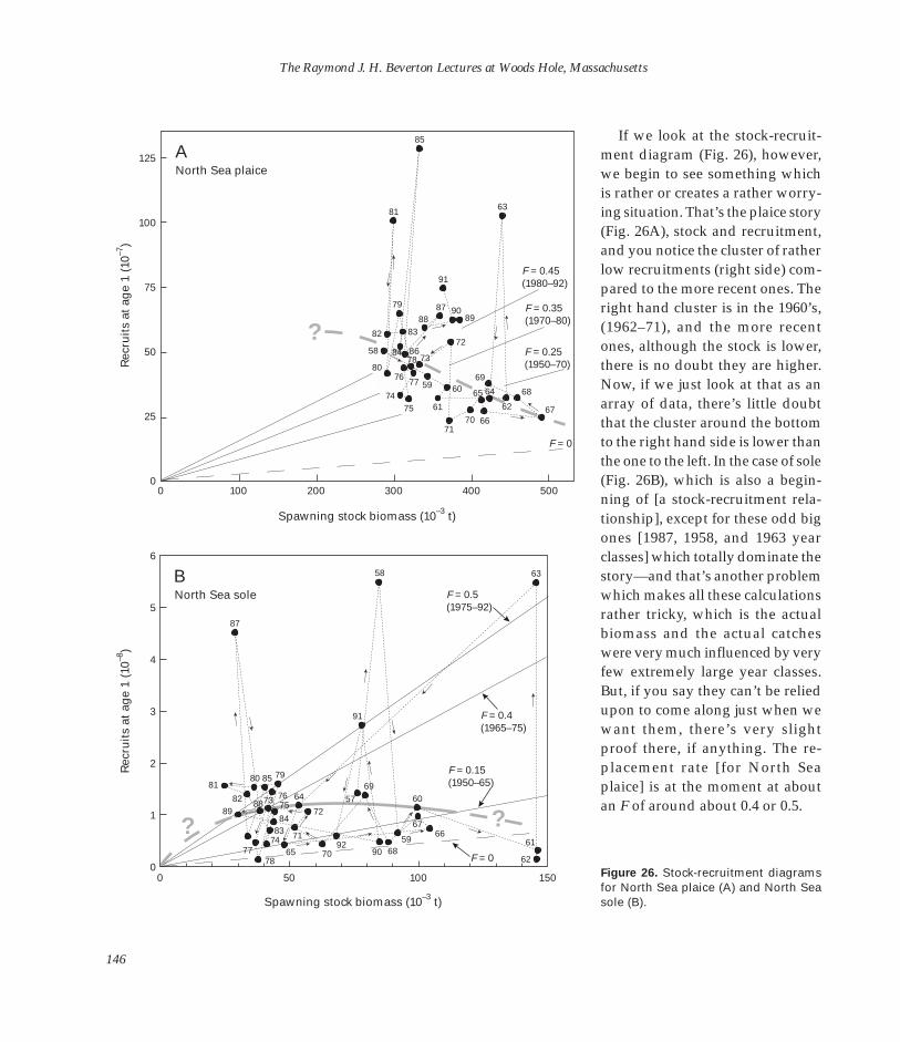
The Raymond J. H. Beverton Lectures at Woods Hole, Massachusetts
Rec
ruit
s at
ag
e 1
(10–8
) R
ecru
its
at a
ge
1 (1
0–7)
125
100
75
50
25
0 0 100 200 300 400 500
Spawning stock biomass (10–3 t)
F = 0.45 (1980–92)
F = 0.35 (1970–80)
F = 0.25 (1950–70)
F = 0
?
North Sea plaice
86
88 87
83
79
81
91
90
80
58 73
82
76
78
77
74 75
59
61
60
71 70 66
62
65
69
64 68
67
89
72
63
85
84
A
6
5
4
3
2
1
0 0 50 100 150
F = 0.4 (1965–75)
F = 0.15 (1950–65)
F = 0.5 (1975–92)
F = 0
? ?
North Sea sole
57
58
59
60
61
62
63
64
65
66 67
68
69
74
7576
77 78
79 80
8889
90
91
92
81
82
83 84
85
87
70
71
72 73
B
Spawning stock biomass (10–3 t)
If we look at the stock-recruitment diagram (Fig. 26), however, we begin to see something which is rather or creates a rather worrying situation. That’s the plaice story (Fig. 26A), stock and recruitment, and you notice the cluster of rather low recruitments (right side) compared to the more recent ones. The right hand cluster is in the 1960’s, (1962–71), and the more recent ones, although the stock is lower, there is no doubt they are higher. Now, if we just look at that as an array of data, there’s little doubt that the cluster around the bottom to the right hand side is lower than the one to the left. In the case of sole (Fig. 26B), which is also a beginning of [a stock-recruitment relationship], except for these odd big ones [1987, 1958, and 1963 year classes] which totally dominate the story—and that’s another problem which makes all these calculations rather tricky, which is the actual biomass and the actual catches were very much influenced by very few extremely large year classes. But, if you say they can’t be relied upon to come along just when we want them, there’s very slight proof there, if anything. The re-placement rate [for North Sea plaice] is at the moment at about an F of around about 0.4 or 0.5.
Figure 26. Stock-recruitment diagrams for North Sea plaice (A) and North Sea sole (B).
146

Lecture 3: Reflections on 100 Years of Fisheries Research
The yield curve for plaice (black solid line, Fig. 27A), as produced by the ICES North Sea Flatfish Working Group (ICES, 1992b), the yield-per-recruit curve, because I suppose recruitment is not thought to be a problem in plaice, gives you an F max somewhere around 0.2. But, if you take this seriously, this question, and try and get the biomass up, you look as if you are going to be suffering a significant drop in recruitment (F = 0.25 line, Fig. 27B). Now, if that were to hap-pen, then you’d get a yield curve looking much more like [the gray solid line] (Fig. 27A). So, actually, in terms of total yield, you wouldn’t be getting what you’d think you would. You’d be down there [about F = 0.2 on the gray solid line] (Fig. 27A). You’d still be better off in terms of catch per unit, of course, but not as well off as you thought you would. Now, Andy, if you put this in, this is a real risk now. This is sort of the decision it seems to me to be how we are going to interpret the cluster (Fig. 26A). They’re all in the 1960’s. The data set so far in that range has never been there twice to check whether you again get a reduced recruitment if you let the biomass go up. I don’t know that there’s an answer to that one, because I can’t see how you can. The 1960’s was a funny decade. You’ve seen all the things that we talked about yesterday about the peculiarity of the 1960s. If the high biomass was
causing the low recruitment, then we have some problems just to know whether we’re right to try and get back in, which is what the advice is at the moment.
Andy Rosenberg In simple terms, if you had to
advise on that, I think you would be ill-served if you said, without a caveat, “Reduce the fishing mortality rate to F max.” On the other hand, you clearly can’t certainly say that if you allow the higher fishing mortality rate, then you will see that benefit of higher recruitment in the long term. In a sense, that would highlight, to me, that you need to put an uncertainty caveat which says, “Proceed cautiously. If you’re going to reduce the harvest rate towards Fmax, then you need to watch out for recruitment, and the only way you can do that is to do it very cautiously. On the other hand, there are good reasons to reduce the harvest rate aside from just yield, and that would be be-cause you have such a poor picture of stock and recruitment on what appears to be the right hand side of the curve only.” It’s rather surprising for plaice to have all that data that appears to be on the right hand side or descending limb of the stock-recruitment curve.
Ray Beverton I hadn’t realized it was coming
out so clear-cut as that. Of course, this is only data from 1957 on-
wards, and this is why it’s so important to go back and put in the historical data. There’s no doubt there have been big changes in plaice. The center of spawning is changed from the Southern Bight just off Lowestoft to the German Bight, as Adriaan Rijnsdorp has re-corded in the Flatfish Working Group report (ICES, 1992b). Completely switched over. There is a lot of spawning way out in the center of the North Sea, which there never was in the old days, so things have been changing in a big way. Over and above all that, there is no doubt that the production has gone up considerably, which you saw from the other one. Of course, the question then is who’s going to be suffering what, if we did, say, go back to there [around F = 0.60, Fig. 27A] and what you’ve got was that drop [difference in yield per recruit be-tween the two yield curves at F = 0.2, Fig. 27A].
If that were really true, you’d be losing (compared with what you thought you were going to get, in terms of yield) not much, only a small percentage, if the gray solid curve were the right one. The problem is you would have had to dismantle some fishing capacity to do it, and that’s the painful thing. It would be easy enough if you could divert the fishing for a few years and say, “Well, go and fish some-thing else while we see what hap-pens to the stock and recruitment
147
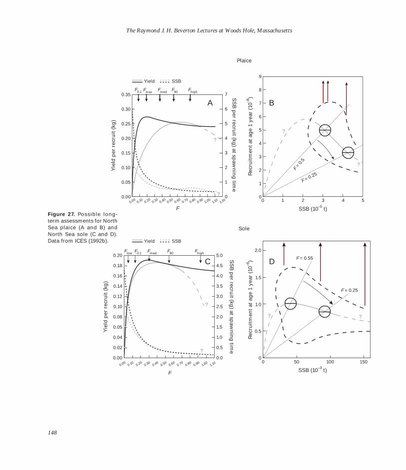
The Raymond J. H. Beverton Lectures at Woods Hole, Massachusetts
Plaice
9 Yield SSB
0.35
?
?
A
F0.1 Fmax Fmed F90 Fhigh
7 8
7 0.30 6
6
0.25 5 5
?
?
F
= 0.
5
F = 0.25
B
0.20 4 4
0.15 3 3
0.10 2 2
0.05 1 1
0.00 0 00 1 2 3 4 5
? ?
F = 0.55
F = 0.25
D
F SSB (10–5 t) Figure 27. Possible long-term assessments for North Sea plaice (A and B) and Sole North Sea sole (C and D). Data from ICES (1992b). Yield SSB
2.0 0.20 5.0
0.18 4.5
0.16 4.0 1.5
0.14 3.5
0.12 3.0
0.10 2.5 1.0
0.08 2.0
0.05 1.5 0.5
0.04 1.0
0.02 0.5
0.00 0.0 0 0 50 100 150
F SSB (10–3 t)
?
?
F0.1 Flow Fmed F90 Fhigh
C
Yie
ld p
er r
ecru
it (
kg)
Yie
ld p
er r
ecru
it (
kg)
SS
B p
er recruit (kg
) at spaw
nin
g tim
e S
SB
per recru
it (kg) at sp
awn
ing
time
Rec
ruit
men
t at
ag
e 1
year
(10
–8)
Rec
ruit
men
t at
ag
e 1
year
(10
–8)
.200.00
0.100.20
0.300.40
0.500.60
0.700.80
0.901.0
01.1
0 1
0.00 0.10
0.20 0.30
0.40 0.50
0.60 0.70
0.80 0.90
1.00
1.10
148
Lecture 3: Reflections on 100 Years of Fisheries Research
situation.” But that takes quite a few years for this sort of fishery to do it. I don’t think, in financial terms, it would be very much to worry about, providing you are there [at F = 0.2 in Fig. 27A] instead of there [F = 0.6], because who’s going to measure the total catch any-way. I mean, total catch is what we all talk about with these curves, but in reality when does the total catch matter? It matters to a country which is totally dependent or very heavily dependent on fishing, but it doesn’t really matter. What much more matters is something like the catch-per-unit-effort rate or the stock-recruitment level. In the sole (Fig. 27C, D), the tendency would be much weaker and it wouldn’t make much difference. I think the difference between the two yield curves is so small, quite honestly, and I don’t think you would worry too much.
Andy Rosenberg If you thought that those 1960’s
and early 1970’s points were from different productivity regimes, if you like, hydrographic issues, and you looked at a stock-recruitment curve in that upper left quadrant which only included the later points, you would draw a curve that would be rather flat topped. That would suggest that the cur-rent fishing mortality rate, if you maintain it there, is probably much riskier. In other words, it’s rather closer to the tangent to the line
since you have no equilibrium point. Then the risk of being close to recruitment overfishing that stock is, in a sense, much more severe than the risk of losing a little bit of yield if that were the true stock-recruitment relationship. But, I guess the problem with the uncertainty analysis is whether it is better to point out the two possibilities and to try to make the argument for caution by pointing out the two possibilities, or better not to confuse people and give what appears to be much clearer or more certain?
Ray Beverton I think the trouble, of course, in
putting across the cautious approach is that it will be seized upon by those who would have to make sacrifices, whichever section of the industry that would be, to do nothing. But, I don’t think, in that case, that one would worry too much. If we really are fishing here [F max on the gray yield curve, Fig. 27A] in-stead of there [Fmax on the black yield curve], I don’t think it’s all that serious, but there might be an-other way of looking at it.
I’ve been trying to see how we could reconcile harvesting strategies, in ideal terms, with what we would like to see happen, with all the modern ideas about biodiversity and all the rest of it. It seems to me that, although for once, economics and that sort of thing are
marching hand in hand, the more timely way of taking that sort of objective would be to say, “Well, we will sacrifice deliberately 5% [of the yield].” That’s a loss of 5 or 6 or 7% of yield which is not going to be tangible to anybody. I sup-pose, theoretically, the processing side, the marketing side, would say, “There’ll be 5 or 6 or 7% less fish going through our hands,” but that’s a pretty intangible sort of thing. But what is tangible is that there is no doubt that the catch per unit effort, put into whatever terms you want to, will be substantially greater if you were there [F0.1 on the gray yield curve] compared with there [F max on the same curve], and what’s more, the biomass would be much greater. That’s the way I think, nowadays, we ought to try and talk about it, so there’ll be no worry about F0.1 in economic terms, but in terms of, “Look, our fishing industry’s contribution to (if you like to put it in simple terms) the ‘Rio principles.’”14 It’s, “Okay, we’ll deliberately fish nevertheless to get the maximum. We’ll deliberately underfish to the extent that
14The United Nations Conference on Environment and Development (UNCED) was convened in Rio de Janeiro in June 1992 to discuss a comprehensive range of environmental issues and to promote the policy of sustainable development. The Conference proclaimed a set of 27 principles (Rio Principles) on the environment and development, designed to promote international cooperation for sustainable development.
149
The Raymond J. H. Beverton Lectures at Woods Hole, Massachusetts
we need only lose 5 or 6 or 7% yield in order to gain more than double the biomass.” That seems to me the sort of argument that we might have to think about in future. Leave the economics [out] on that one. The fishermen would be quite happy with that, except those who are going to lose out. It will be those concerned with the shipbuilding side, with the gear, all that has to do with the catching side, who will miss out because they’ll have to run with a smaller fleet, and smaller manpower, and everything else.
I’m talking [here of] a long-term objective. I’m not talking of some-thing you’d get at straightaway. But it does seem to me that those sort of redefinition of familiar objectives may be timely if we’re going to keep pace with some of the modern attitudes to the way certain of our environmental lobbyists are thinking in terms of attitudes that anything to do with commercial fishing is anathema. We may have to find ways [to reduce fishing pressure], and if so, then it points to literally aiming at a point like that [F0.1 on the gray yield curve in Fig. 27A] while we’re trying to get to the sustainable maxi-mum. Don’t you think so, Andy? I know it’s all a lot of theoretical talk.
Andy Rosenberg I don’t think it is, in fact. Unfor
tunately, I think that sometimes the argument does come down to 5%.
People will make a fierce stand around here at 5%. They start bringing their children into it, and their houses, having to eat dog-food, and everything else. But in principle, I don’t anticipate at all a sensible way to approach it.
Steve Murawski I think it almost comes full circle
to Bob Edward’s comments about the role of scientists in defining societal objectives and certainly pushing societal objectives in a much more of an advocacy role. Based on the first century of population dynamics research, I think we understand the effect of single-species fisheries regimes on quantities such as yield maximization, effect on biomass ability, and a variety of single-species parameters. The traditional optimization points have been places on the eumetric fishing curve, but they come at great risk. We understand these things to a much greater degree than our para-professional managers, who are out there, and certainly the general public. I think we are almost obliged to “take it on the road,” as it were, and to at least get the public more familiar with the great risks that the managers seem to be willing to accept in terms of the collapse of these stocks and their impacts on society in general. I know we have a very uneasy time dealing with ourselves as scientists, in an advocacy role. On the other hand, if it wasn’t for the
dawn of the environmentalist, we would be on one end of the lever and all the fishing industry would be on the other end. I think the nice thing about having this great interest by environmentalists is that we can sort of subtly shift to the center and play more of a fair-broker-of-information role, or try to. I know Vaughn and I have, in the last 5–10 years, really gotten our-selves into some tight pickles trying to encourage this without re-ally having ourselves perceived as being very strident in this whole area.
Vaughn Anthony There is a big gap though, I
think, in this kind of advice and however we come forward with advice to the managers and [with] what they really need to manage. Managers are not having any problem with what we say in its accuracy. They think we know what’s going on; they agree with what we say. We’re not giving them the information they really need to manage, because they want to know how they’re going to get over the social problems of man-aging, recovering the stocks, reducing catches, and so forth. I think we’re making a big mistake in not giving them the information they need to manage, which is the social aspect. How do you lay on a management program and have people “survive” or change their lifestyle or move into a different
150
Lecture 3: Reflections on 100 Years of Fisheries Research
way of operating when there’s a little less fish out there than there used to be? How do they function, how do they live, how do they change their lifestyle? We don’t even give them any information on any of that stuff, so they’re afraid to move forward to do what’s responsible because they don’t know how to do it.
There’s a big gap between science and biology and fish management, and I think we’re making a mistake if we think there’s not much of a gap between management and biology. I think biology is straightforward and easy and is not much of a problem. Even these things [the science] are not much of a problem. No one will give us grief about them, but trying to get managers to actually put some-thing in place that affects people’s lives and how they do their day-to-day activity requires a lot more information, different kinds of in-formation, not just economic, but social information which we are not giving them and helping them manage. I think that’s where some-body’s making a mistake. It’s not the stock assessment science. We are not socially oriented to do that, but it’s a whole area we are not providing information on, and they don’t know how to proceed. Some-body has to step in and give them the information and say, “If you want to manage along these lines, here’s some information, here’s
what will happen, here’s the responses, and here’s a lot of data dealing with the lives of people.” We’re not doing it, and that’s where the problem is with fish management, as far as I’m concerned, not whether it’s F max, or growth over-fishing, or recruitment overfishing.
Steve Murawski If I could be so bold, I’d say that
the first century of fisheries re-search has basically been a golden age of single-species population dynamics. I think Vaughn is exactly right that we’ve come to the realization that we can’t manage fisheries for the sake of fish. The issues seems to be relatively clear to the point where we are trying to clean up and evaluate our variances, etc. But, there is a whole realm of fisheries science in which, even in terms of the evolution of this laboratory and some of the new people who have come on, a whole realm of science in economics and social science which, even though seminal papers were written in the 1950’s, has a long developmental period that perhaps, I hope, is not as long as the developmental period in population dynamics. But, I think we may have actually seen the height of population dynamics research on a single-species basis. Now we may be entering into an era of social and economic analysis.
Vaughn Anthony [Fishery management] council
people say to us all the time, “We don’t argue with anything you guys say. We believe everything you say. So what! We’re scared to put in a management program be-cause we just don’t know how to get it done. We just walk away.”
Marvin Grosslein It isn’t a lack of information so
much as it is a lack of political will. I think the environmental movement is gradually, perhaps, em-powering administrators, and we recognize that the public does eventually see the environmental policy as an issue of sustainability. I think we’re becoming more understood by the public, and per-haps the political-will issue may be overcome more easily, we hope, in the future. Until that happens, no amount of information is going to change anything.
Ray Beverton I think Steve has put his finger
on the button, really. I’ve been talking about two species there, but they can probably be perfectly well treated as a single species. But if you did it on some of the gadoids, and I must admit I haven’t fully thought out to myself what you would aim at, you would probably assume, “Well, we’ll aim at some-thing on the safe side of F max.” What is that in a mixed fishery? Is there such a thing in an interacting species complex?
151

The Raymond J. H. Beverton Lectures at Woods Hole, Massachusetts
There is such a thing, I expect. I’ve asked Lowestoft, I’ve asked John Pope15, “Can you give me sort of a combined yield curve?” He said, “Oh, I can’t do that. We’ve already looked at that and can’t think along those lines now.” I know what he means. It depends which mix of fishing effort is going to be on which species, as well as the interaction between them. But there has to be something there. I mean, they will fish the mix in some way or other, and there is going to be a response, and it seems to me that we’ve got to have some-where a hand in that situation. The Norwegians will, but there are only three species to balance. They’re going to do a three-ball juggling act of the three major species. Whether we can do it in a more complex one, I don’t know.
Andy Rosenberg A couple of things. In the multi-
species case, the question has to be much more specific. You can no longer say, “What’s the optimum or maximum sustainable yield?” We’re not to the point where we’re being asked specific questions until somebody says, “Well, how should we fish?” You have to say, “What do you mean? After you fish, what do you want to achieve?” That objective has to be very specific in a multispecies case, whereas
15Fisheries scientist at Lowestoft Laboratory, U.K.
we could generally, in a single-species case, say, “Well, at least you want to get as much catch as you can out of this thing without being too risky about it.” I don’t disagree with the importance of the economic information for the economic analysis, but I don’t think we should lose sight of the fact that, in general, the managers, being either political managers or, in our case, the [fishery management] councils, say that they’re the ones who know the fishing industry and the fishing business and the fishing communities. They’re there to represent those communities and those social factors and economic factors within the interest groups. In a sense, they’re supposed to be providing that side of the equation, given the biological advice.
I don’t disagree with Vaughn that, in many cases, they’re now saying, “OK, give us more, we need more, we need more information.” But it’s certainly true that that was the information that fishery management councils were in-tended to bring to the table in making their management decisions. It was not viewed as, “Well, the scientists didn’t give us enough.” They weren’t viewed as a collection of twelve reasonably bright people who would assimilate any of the information that came to them. They came to the table with expertise. So, I’m not quite sure that it’s the case that none of that
information was in front of them by which to proceed. The difficulty was that it all focused on the biological information for a long time, and they essentially were not accepting the biological principle and then getting on with the issues of management.
Steve Murawski I think ultimately, for example,
in the case of New England ground-fish (which I’m sure you’re alluding to), getting over the hump of actually making a management decision was based on whether or not, in an economic sense in the long term, it paid off, because people make a lot of money on collapsed stocks because the value per pound is quite high. Ultimately, there was a technical question whether or not the net benefits to society exceeded the tremendous economic cost, not necessarily the social cost. So, I think there is room for technical analysis.
Andy Rosenberg I think there is too. I’m not say
ing that there isn’t, but I do not think that it’s been left out.
Fred Serchuk I just want to follow up on what
Andy said, because I think the economics are not up front, nor are the social [sciences], but they are in there of a sort. When you say management makes short-term decisions, they are just externalizing a
152

Lecture 3: Reflections on 100 Years of Fisheries Research
socioeconomic cost away. That is, they are responding to the political exigencies of the day. To close down a fishery? No, politics comes in to play. Nobody has actually considered the long-term cost. What Ray is basically saying is, if you go back and take a retrospective look, you might be able to say, “Had we taken this action, then you would get an idea of the magnitude of what the benefits would be and what the costs would have been at that point [by] doing it over the long term.” So, I think that retrospectively is really quite a nice way to go.
In terms of fisheries or fisheries science only being a small component of it, I recall a remark that Jakob Jakobsson16 made several years ago at an ICES meeting where he said, “When we try to predicate our management based on a strong scientific basis, as they did for herring, as they did for capelin and other stocks, and in many cases had very modest fishing mortality levels, such as F0.1, or very substantial minimum biomass levels, we get into trouble. When we deviated from a biological basis, as we did for the cod stock, and put most of the decision weight on socioeconomic factors, we got into problems.” Here’s a case where, in Iceland, fisheries are
16Director of the Icelandic Marine Research Institute in Reykjavik.
important and they deal with 10 or 15 different stocks, and the cod stock is one of the most important. When they started basing decisions on socioeconomic information, at least discounting it in the long term, they got themselves into a mess.
Ray Beverton If I can just comment on the
multispecies [issue], it seems to me that it blurs the range of clarity in the middle, but it doesn’t blur the extremes. If you’re up to an F of 1 on cod, irrespective of whether it’s a multispecies [fishery] or not, it’s almost certainly not going to be a very sensible thing to do. Conversely, there’s no point in getting too far back the other way. It does mean that there’s a wider area in the middle which you have to say, if you know enough about it, “Well, you can have a certain proportion of that plus that plus, or if you do that, you can have that, plus that, etc.” It doesn’t alter the general impression, though, that excessive fishing is almost certainly going to be undesirable on every ground, and that there’s quite a lot of present situations we’re in whether it’s your haddock—I mean your had-dock is not a single species, but you can be jolly sure you’re overfishing it [or another species]—so, I don’t think we should allow the multispecies [issues] to frighten us. It’ll blur the middle, but it won’t prevent the really brink side of sci
ence from being pretty realistic. It may be just a little more difficult to be sure where you are at the edges, but you know where you are already on some of them. You don’t need to worry about multi-species [management] for that point. Isn’t that fair, Andy?
Fred Serchuk What about protection? I’m
thinking about marine mammals now—the seals. This is a real big problem that we have in fisheries.
Ray Beverton We haven’t seen it quite as
strong as you have, or potentially have. I think the Norwegians are going to have to now put the minke whale and the others into their equation in a big way. They won’t be able to leave them out of their Barents Sea story. Of course, I think we must, as fisheries scientists, put this into the equation really to make sure we have it right. What is done about it is another matter. [As for] the question of the economics and the politics, I think what we have to get across is that, unlike farming, the only way that we can influence the future replenishment of a stock is by con-trolling the harvesting rate. The trouble is that the harvesting rate is played fast and loosely by the economists who don’t realize that—they think you can manipulate whatever you like and it doesn’t make any difference in the
153
The Raymond J. H. Beverton Lectures at Woods Hole, Massachusetts
long term. We seem to fail to get it across, and it does matter, and, unlike farming, you can’t step up effort.
I don’t know whether you have yet read Mike Holden’s book on the Common Fisheries Policy (Holden, 1993). If you haven’t, you’d be well advised to do so. It’s an extraordinary book because it’s a mixture of the factual account, the pretty glaring account, and he’s drawn aside the curtains and shown you some of what he called ultimately “horse dealing,” [which] was going on all the time. It was an apologia, for clearly he feels he’s failed [as a fisheries manager]. He thinks he’s being criticized for failing, which I don’t think was true actually, but he feels he’s responsible. He tries to make a gloss of it, that it wasn’t really a failure, but in fact it was a ghastly failure. The reasons for it were very special. They’re not the sort of reasons you would place here. I won’t go into details, but will just say that when NEAFC collapsed because of the 200-mile extension in the mid 1970’s, the E.C. hadn’t really got-ten a common fisheries policy at all. The U.K. only had just joined, and Denmark had only just joined in 1974 or 1975, so we were new boys in it, and yet we were powerful players in any fisheries policy.
The move to have a fisheries policy came from the Italians and
the French who wanted a market-oriented expansion. The idea was, “Look, we said we’ve got to make ourselves self-sufficient in the European Community in agriculture and fisheries. We’ve done it for agriculture.” What they’d done was to create enormous surpluses, of course, which were grossly, entirely wasteful. I mean, it was ghastly business really, when you have mountains, millions of tons, of butter that nobody can do any-thing with. But, leaving that aside, at least economically, provided you subsidize your farming, which was heavily unraveled, it was at least a coherent exercise. They set out to do the same for fishing. “Let’s double the fishing.” So, we doubled the fishing power. So, everything was subsidized. Countries were building new ships with E.C. money when they should have done the opposite. They took not the slightest notice of decades of ICES advice through NEAFC, through the Overfishing Conven-tion17.
There wasn’t even a [fisheries] scientist in the Directorate until Mike Holden went there. Because the influential countries were only
17The 1946 Convention for the Regulation of Meshes of Fishing Nets and the Size Limits of Fish, which came into force in 1953 and led to the establishment of the Permanent Commission, which was re-named 10 years later the North-East Atlantic Fisheries Commission (NEAFC).
really on the edge at that point, presumably we didn’t exercise our responsibility—I say “we,” the U.K. for a start—I wasn’t there. I was with NERC; I wasn’t at Lowestoft then. I know Cushing got totally and utterly frustrated with what was going on there and really almost opted out of it half the time. The net result was, not for that reason but for other reasons, the whole thing was set up on an expansionist policy when the exact opposite should have happened. They [the fisheries] should have been contracting, and it’s only now [mid 1990’s] that they’ve had to “bite the bullet” and are starting to offer subsidies for removal of a few percent of fishing power. So, there’s a case, maybe it’s a special case, that wouldn’t be repeated in most other countries. It’s a special case of market-oriented and political forces actually dominating [fishery management decisions]. It wasn’t a question of where on the yield curve you were. There’s no such thing as a yield curve; you just expand. It’s a terrible lesson and a tragic lesson really, as far as the North Sea is concerned, not as bad as a truly collapsed fishery then, but still as an exercise in sensible husbandry of natural resources, a pretty poor record.
Steve Clark We have an identical one; a
pretty poor record.
154
Lecture 3: Reflections on 100 Years of Fisheries Research
Ray Beverton So, somehow or other, there was
obviously no scientific message getting through. Who’s fault it was I don’t think you can say, because it was a special situation. It wasn’t the scientific message not getting through at all. It wasn’t that it was being disregarded, or it wasn’t a question of no risk analysis, it was just not there at all.
Steve Murawski I think one more question from
Paul. I think we’ve exercised your capacity as long as we can.
Paul Rago I just wanted to ask you one of
the questions you partially answered. I would like to hear your thoughts on the idea of multi-species management and, before we completely understand it, if we ever will, the idea of managing on the basis of the weakest species or a weak species which is collapsed and managing around that. One that comes to mind is Pacific halibut and the idea of other fisheries being restricted on the basis of the bycatch of that species in those fisheries. When those situations occur, everyone else benefits. Per-haps haddock or yellowtail flounder would be an appropriate species here from which you could base a multispecies management on the weakest component and then bring everybody else up along the way.
Ray Beverton That might prove to be quite a
useful way into it. If you’re talking about using your haddock as an example, as I was saying, I hardly think you need worry initially about the multispecies aspect to it. You just get cracking on it some-how or other. It’s way outside the range of sensitivity on a multi-species basis, but when you are getting everything growing back from the brink and getting more to-wards being generally abundant, I think in a really complex fishery, of which yours may not be even the most complicated, some of the tropicals would be much more so, I don’t think there is any way you can manage without extraordinary difficulty and complexity and expense trying to pick out individual species and trying to treat them separately. You have to try and take a by-and-large level not too excessive of fishing effort and let them go. What they’ll do is overfish to some extent, depending on market demands and local temporary abundance or shortage, and under-fish others. After a bit, they’ll change around and switch another way. If you can get it to that sort of situation and let the fishermen go, you don’t have to interfere with their activity; we can let them go. As long as there aren’t too many of them, they can’t do dramatic harm. If they do, they’ll soon realize that they’re not getting much out of that and they’ll switch to
another one once they can be taught to switch around.
I think there comes a point in some of these complicated fisheries when expecting to get an objective that is too sharply defined, trying to fine-tune it by management, becomes an unreal objective. Trying to do it, I think, will make our science less credible than need be. We’re asking too much, just as we would refuse to make a prediction of what the yield curve would be 10 years off, because we know we can’t. I think we just have to acknowledge that there are some things we can’t predict and it would be foolish to try and do so.
One of the difficulties with all the TAC business that we’ve had on the European scene, and you’ve probably had the same, is that you get a prediction wrong and that destroys the credibility. The 1985 year class in North Sea haddock was much stronger than we thought it was and it upset all the quotas and TAC’s. They had haddock running out of their ears and fisher-men said, “These bloody scientists, they’re telling us there are no had-dock, they don’t know what they’re talking about.” It was on television, it was everywhere; I was down at Lowestoft not long ago, and they said it has done more harm, that one miscalculation, than the decades of attempts to try to get it right. So, to some extent, we should
155

The Raymond J. H. Beverton Lectures at Woods Hole, Massachusetts
only aim at targets which we can reach scientifically as well and not try and pretend that we can be absolutely precise about what the catch is going to be, even for a short time.
All of this comes back to not having to make TAC’s the dominant idol that everybody goes to. I know it’s easy to say and difficult to do, but in the end, if only we can get there, it would be worth it. TAC’s will no longer be the absolute sort of cutting edge so sharply as it is at the moment. You can let them get on with it and have a re-view every few years of what has happened to F—that’s what matters—on the understanding that if it’s gone up above a certain point, there’d have to be a redistribution
or running-down schedule put in over the next 5 years. There’d be the money, if you have a good rental system, to pay for that. I think that’s the sort of schedule. In the meantime, you let them get on with it, and they’re not hedged about by this, that, or the other thing and they can get on and fish as they like. It won’t be perfect, but it won’t be a disaster, and it may be that’s the best way of gradually edging them into a more sensible husbandry approach, which will satisfy some of the more reasonable members of the environmental lobby.
Steve Murawski I think that’s a long argument
for effort control. Thank you.
Ray Beverton I hope you found it enjoyable
and helpful, and thank you for being such a good audience, yesterday as well.
Steve Murawski On behalf of the NMFS North-
east Fisheries Science Center, I’d really like to thank you for obliging us with three outstanding lectures. I know we have all been impressed, certainly, by your endurance and putting up with us for two grueling days and a couple of parties.
Ray Beverton Thank you, Steve.
156

Lecture 3: Reflections on 100 Years of Fisheries Research
Literature Cited
Andersen, K. P., and E. Ursin. 1977. A multispecies extension to the Beverton and Holt theory, with accounts of phosphorus circulation and primary production. Meddr. Danm. Fisk. og Havunders. N.S. 7:319–435.
Baranov, F. I. 1918. On the question of the biological basis of fisheries. Nauchn. Issled. Iktiol. Inst. Izv. 1:81–128.
Beverton, R. J. H., and S. J. Holt. 1957. On the dynamics of exploited fish populations. Fish. Invest., Lond., Ser. 2, 19, 533 p.
Beverton, R. J. H., and S. J. Holt. 1993. On the dynamics of exploited fish populations. Chapman & Hall, Lond., 533 p.
Bückmann, A. 1936. Scholle (Pleuronectes platessa). Die relative stärke der einzelnen jahrgänge in verschiedenen meeresteilen. Rapp. P.-v. Cons. Perm. Int. Explor. Mer 101(III, 7):3–15.
Clark, R. S. 1936. Age composition of haddock in European waters. Rapp. P.-v. Cons. Perm. Int. Explor. Mer 101 (III, 2):3–7.
Daan, N., H. J. L. Heessen, and J. G. Pope. 1994. Changes in the North Sea cod stock during the twentieth century. ICES Mar. Sci. Symp. 198:229–243.
Edser, T. 1908. Note on the number of plaice at each length, in certain samples from the southern part of the North Sea, 1906. J. Roy. Stat. Soc. 71:686–690.
Garstang, W. 1900. The impoverishment of the sea. J. Mar. Biol. Assoc. U.K., N.S. 6:1–69.
Graham, M. 1935. Modern theory of exploiting a fishery, and application to North Sea trawling. J. Cons. Int. Explor. Mer 10:264–274.
Graham, M. 1943. The fish gate. Faber and Faber, Ltd., Lond., 196 p.
Gulland, J. A. 1965. Estimation of mortality rates. Annex to Arctic Fisheries Working Group. Report of meeting in Hamburg, 18–23 Jan. 1965. ICES C.M. 1965 Gadoid Fish Committee, No. 3, 9 p.
Harris, S. 1992. Chalk up another one: the best of Sidney Harris. AAAS Press, Wash., D.C., 146 p.
Heincke, F. 1913. Investigations on the plaice. General report. I. The plaice fishery and protective regulations. Rapp. P.-v. Réun. Cons. Perm. Int. Explor. Mer 17:1–153.
Hilborn, R. 1979. Comparison of fisheries control systems that utilize catch and effort data. J. Fish. Res. Bd. Can. 36:1477–1489.
Hilborn, R. 1985. Fleet dynamics and individual variations: why some people catch more fish than others. Can J. Fish. Aquat. Sci. 42:2–13.
Hjort, J. 1914. Fluctuations in the great fisheries of northern Europe reviewed in the light of biological research. Rapp. P.-v. Cons. Perm. Int. Explor. Mer 20: 1–228.
Holden, M. J. 1993. The common fisheries policy: origin, evaluation and future. Fishing News Books, Oxford, 274 p.
Hulme, H. R., R. J. H. Beverton, and S. J. Holt. 1947. Population studies in fisheries biology. Nature 159:714–715.
ICES. 1992a. Report of the Study Group on Ecosystem Effects of Fishing Activities. ICES C.M. 1992/G:11, 144 p.
ICES. 1992b. Report of the North Sea Flatfish Working Group. ICES C.M. 1992/Assess:6, 220 p.
Jones, R. 1961. The assessment of the long term effects of changes in gear selectivity and fishing effort. Marine Re-search (Scotland) 2:1–19.
Jones, R. 1964. Estimating population size from commercial statistics when fishing mortality varies with age. Rapp. P.-v. Réun. Cons. Perm. Int. Explor. Mer 155: 210–214.
Lee, A. J. 1992. The Ministry of Agriculture, Fisheries and Food’s Director-ate of Fisheries Research: its origins and development. Minist. Agric. Fish. Food, Dir. Fish. Res. Engl. Wales, Lowestoft, 332 p.
Lasker, R., and K. Sherman (Editors). 1981. The early life history of fish: re-cent studies. The Second ICES Symposium, Woods Hole, 2–5 April 1979. Rapp. P-v. Réun. Cons. Perm. Int. Explor. Mer 178, 607 p.
Mardon, M. 1994. Madam President. Sierra. The Magazine of the Sierra Club. January/February 1994, p. 17.
May, R. M. (Editor). 1984. Exploitation of marine communities: report of Dahlem workshop on Exploitation of Marine Communities, Berlin, April 1– 6, 1984. Springer-Verlag, Berlin, 366 p.
157

The Raymond J. H. Beverton Lectures at Woods Hole, Massachusetts
Moran, P. A. P. 1950. Some remarks on animal population dynamics. Biometrics 6: 250–258.
Murphy, G. I. 1965. A solution of the catch equation. J. Fish. Res. Board Can. 22:191–202.
Ottestad, P. 1933. A mathematical method for the study of growth. Essays on population. Hvalråd. Skr. 7:30–54.
Paloheimo, J. E., and L. M. Dickie. 1964. Abundance and fishing success. Rapp. P.-v. Réun. Cons. Perm. Int. Explor. Mer 155:152–163.
Parrish, B. B. (Editor). 1973. Fish stocks and recruitment. Proceedings of a Symposium held in Aarhus 7–10 July 1970. Rapp P.-v. Réun. Cons. Perm. Int. Explor. Mer 164, 372 p.
Pearl, R. 1925. The biology of population growth. A. A. Knopf, N.Y., 260 p.
Ricker, W. E. 1954. Stock and recruitment. J. Fish. Res. Board Can. 11:559– 623.
Russell, E. S. 1931. Some theoretical considerations on the “overfishing” problem. J. Cons. Int. Explor. Mer 6: 3–20.
Saville, A. (Editor). 1980. The assessment and management of pelagic fish stocks. A Symposium held in Aberdeen, 3–7 July 1978. Rapp P.-v. Réun. Cons. Perm. Int. Explor. Mer 177, 517 p.
Schaefer, M. B. 1954. Some aspects of the dynamics of populations important to the management of the commercial marine fisheries. Inter-Amer. Trop. Tuna Comm. Bull. 1(2):26-56.
Sissenwine, M. P., and A. A. Rosenberg. 1993. Marine fisheries at a critical juncture. Fisheries (Bethesda) 18(10):6–14.
Smith, T. D. 1994. Scaling fisheries: the science of measuring the effects of fishing, 1855–1955. Camb. Univ. Press, Camb. 392 p.
Sund, O. 1936. The fluctuations in the European stocks of cod. Rapp. P.-v. Réun. Cons. Perm. Int. Explor. Mer 101 (III, 1):2–18.
Templeman, W. 1972. Year-class success in some North Atlantic stocks of cod and haddock. Int. Comm. Northw. Atl. Fish., Spec. Publ. 8:223–238.
Thompson, W. F., and F. H. Bell. 1934. Biological statistics of the Pacific halibut fishery. 2. Effect of changes in in-tensity upon total yield and yield per unit of gear. Rep. Int. Fish. Comm. 8, 49 p.
von Bertalanffy, L. 1938. A quantitative theory of organic growth. Human Biol. 10(2):181–213.
von Bertalanffy, L. 1949. Problems of organic growth. Nature 163:156–158.
Walters, C. J. 1986. Adaptive management of renewable resources. Macmillan, N.Y., 374 p.
158
Appendix
Common and Scientific
Names of Species


The following is a listing of the common and scientific names of fish, shellfish, and marine mammals mentioned in this book. The species are listed in the order first mentioned. The scientific names printed in each lecture use the same spelling of Raymond Beverton’s original figures and of the figures from the cited literature.
Atlantic herring, Clupea harengusPacific herring, Clupea pallasiEuropean pilchard, Sardina pilchardusSprat, Sprattus sprattusCalifornia sardine, Sardinops sagax caeruleaSpanish sardine, Sardinella auritaSouth African pilchard, Sardinops ocellatusPeruvian anchoveta, Engraulis ringensEuropean anchovy, Engraulis encrasicolusPacific anchoveta, Cetengraulis mysticetusPacific or chub mackerel, Scomber japonicusAtlantic mackerel, Scomber scombrusBluefin tuna, Thunnus thynnusCape hake, Merluccius capensisSilver hake, Merluccius bilinearisHaddock, Melanogrammus aeglefinusPollock or saithe, Pollachius virensWhiting, Merlangius merlangusAtlantic cod, Gadus morhuaPacific cod, Gadus macrocephalusGreenland cod, Gadus ogacPolar cod, Boregadus saidaPoor cod, Trisopterus minutusNorway pout, Trisopterus esmarkiiRedfish, Sebastes spp.Pacific ocean perch, Sebastes alutusSilvergray rockfish, Sebastes brevispinisYellowtail rockfish, Sebastes flavidusCanary rockfish, Sebastes pinnigerYellowmouth rockfish, Sebastes reediSharpchin rockfish, Sebastes zacentrusRedstripe rockfish, Sebastes prorigerPuget Sound rockfish, Sebastes emphaeus
Olive rockfish, Sebastes serranoidesAcadian redfish, Sebastes fasciatusDeepwater redfish, Sebastes mentellaPlaice, Pleuronectes platessa1
North Sea sole, Solea soleaAmerican plaice, Hippoglossus platessoidesGreenland halibut, Reinhardtius hippoglossoidesAtlantic halibut, Hippoglossus hippoglossusPacific halibut, Hippoglossus stenolepisYellowtail flounder, Limanda ferruginea2
Witch flounder, Glyptocephalus cynoglossusCommon sole, Solea vulgarisPetrale sole, Eopsetta jordaniLarge-tooth flounders, Paralichthys spp.Long-snouted flounder, Ammotretis rostratusJapanese flounder, Paralichthys olivaceusStarry flounder, Platichthys stellatusWinter flounder, Pleuronectes americanusGreenback flounder, Rhombosolea tapirinaFlatfish (flounder species)Common skate, Raja batisSpiny dogfish, Squalus acanthiasStriped bass, Morone saxatilisCapelin, Mallotus villosusSandeel, Ammodytes spp.Atlantic salmon, Salmo salarTrout, Salmo spp.Walleye, Stizostedion vitreumPrawns, Pandalus borealisHarp seal Phoca groenlandicaHooded seal, Cystophora cristataMinke whale, Balaenoptera acutorostrata
1Now Platessa platessa 2Now Pleuronectes ferrugineus.
161