The rainfall erosivity factor in the Czech Republic and its uncertainty · 2016-10-25 · M. Hanel et al.: The rainfall erosivity factor in the Czech Republic 4309 and discussed in

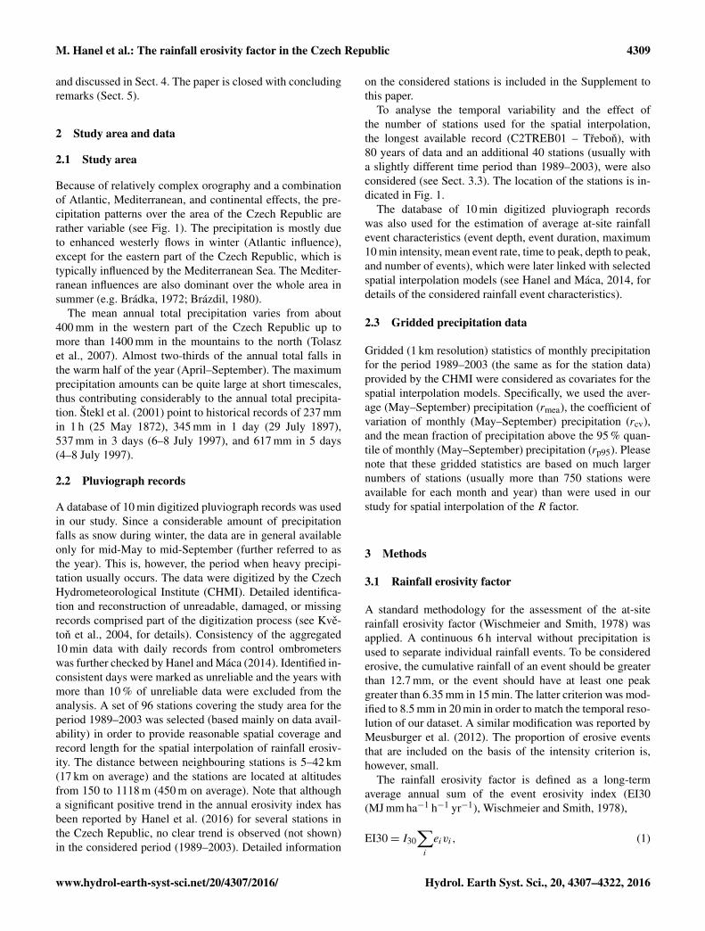
Hydrol. Earth Syst. Sci., 20, 4307–4322, 2016www.hydrol-earth-syst-sci.net/20/4307/2016/doi:10.5194/hess-20-4307-2016© Author(s) 2016. CC Attribution 3.0 License.

The rainfall erosivity factor in the Czech Republicand its uncertaintyMartin Hanel1,2, Petr Máca1, Petr Bašta1, Radek Vlnas1, and Pavel Pech1

1Faculty of Environmental Sciences, Czech University of Life Sciences, Kamýcká 1176, Prague 6, Czech Republic2T. G. Masaryk Water Research Institute, Podbabská 30, Prague 6, Czech Republic

Correspondence to: Martin Hanel ([email protected])

Received: 6 April 2016 – Published in Hydrol. Earth Syst. Sci. Discuss.: 18 April 2016Revised: 11 July 2016 – Accepted: 9 October 2016 – Published: 25 October 2016

Abstract. In the present paper, the rainfall erosivity factor(R factor) for the area of the Czech Republic is assessed.Based on 10 min data for 96 stations and correspondingR factor estimates, a number of spatial interpolation meth-ods are applied and cross-validated. These methods includeinverse distance weighting, standard, ordinary, and regres-sion kriging with parameters estimated by the method ofmoments and restricted maximum likelihood, and a gener-alized least-squares (GLS) model. For the regression-basedmethods, various statistics of monthly precipitation as wellas geographical indices are considered as covariates. In ad-dition to the uncertainty originating from spatial interpo-lation, the uncertainty due to estimation of the rainfall ki-netic energy (needed for calculation of the R factor) as wellas the effect of record length and spatial coverage are alsoaddressed. Finally, the contribution of each source of un-certainty is quantified. The average R factor for the areaof the Czech Republic is 640 MJ ha−1 mm h−1, with val-ues for the individual stations ranging between 320 and1520 MJ ha−1 mm h−1. Among various spatial interpolationmethods, the GLS model relating the R factor to the alti-tude, longitude, mean precipitation, and mean fraction of pre-cipitation above the 95th percentile of monthly precipitationperformed best. Application of the GLS model also reducedthe uncertainty due to the record length, which is substantialwhen the R factor is estimated for individual sites. Our re-sults revealed that reasonable estimates of the R factor canbe obtained even from relatively short records (15–20 years),provided sufficient spatial coverage and covariates are avail-able.

1 Introduction

Erosion is a natural geological phenomenon resulting fromthe removal and transportation of soil particles by water,wind, ice, and gravity. Soil erosion by water is a widespreadproblem throughout Europe (Van der Knijff et al., 2000;Panagos et al., 2015). Erosion is usually driven by a combi-nation of factors like climate (e.g. long dry periods followedby heavy rainfall), topography (steep slopes), inappropriateland use, land cover patterns (e.g. sparse vegetation), ecolog-ical disasters (e.g. forest fires), and soil characteristics (e.g. athin layer of topsoil, a silty texture, or low organic mattercontent).

Although measurements of soil erosion exist, they are of-ten used as a basis for development, modification, or veri-fication of soil erosion models (applicable at larger scales),which relate soil loss to indicators of relevant factors. Aclassic example is the Universal Soil Loss Equation (USLE,Wischmeier and Smith, 1978) or the Revised USLE (Renardet al., 1997). Both methods express the long-term average an-nual soil loss as a product of rainfall erosivity factor (R fac-tor), soil erodibility factor, slope length factor, slope steep-ness factor, cover-management factor, and support practicefactor. The experimental data indicate that when factors otherthan rainfall are held constant, soil losses from cultivatedfields are directly proportional to an erosivity index (EI30)calculated as the total rainfall kinetic energy times the max-imum 30 min intensity (Renard et al., 1997). The R factor isthen obtained as a long-term average annual rainfall erosiv-ity index. In addition to a point estimate of the R factor, a

Published by Copernicus Publications on behalf of the European Geosciences Union.

4308 M. Hanel et al.: The rainfall erosivity factor in the Czech Republic

spatial information (map) is often required for practical pur-poses. A number of such maps have been released recently atnational (Lu and Yu, 2002; Yin et al., 2007; Bonilla and Vi-dal, 2011; Oliveira et al., 2013; Borrelli et al., 2016; Panagoset al., 2016a; Meddi et al., 2016) or larger (Panagos et al.,2015) scales.

Because of large spatiotemporal variability of rainfall,long records from a dense network of stations are in generalrequired in order to provide reliable estimates of the R factorand/or to develop rainfall erosivity maps. For instance, Wis-chmeier and Smith (1978) or Verstraeten et al. (2006) rec-ommend at least 22 years of data to be used for estimationof the R factor. On the other hand, lack of high-resolutionrainfall data in combination with a need for soil erosion riskassessment often leads to situations where the R factor hasto be estimated from shorter records. For instance, a numberof stations used recently for the derivation of rainfall ero-sivity maps for Europe (Panagos et al., 2015) were shorterthan 20 years and several records shorter than 10 years wereconsidered. Similarly, the comparison of the spatial interpo-lation methods in the Ebro Basin (Angulo-Martínez et al.,2009) was based on 10 years of data (for a large number ofstations) and Catari et al. (2011) assessed the uncertainty inthe estimated R factor considering a 13-year record for eightstations. In general, the uncertainty in the estimated R fac-tor increases as the length of the available record decreases,but can be reduced by combination of data from differentsites (Catari et al., 2011) or by considering covariates thatare better sampled and/or whose variation over space andtime is smaller (Goovaerts, 1999). For the spatial interpo-lation of the R factor, variables like longitude, latitude, andelevation (Goovaerts, 1999; Angulo-Martínez et al., 2009) orlong-term precipitation (Lee and Lin, 2014) are often consid-ered.

In addition to spatial and temporal variability, the expres-sions for the rainfall kinetic energy (needed for estimation ofthe erosivity index) and spatial interpolation are also relevantsources of uncertainty for the development of an R factormap. The rainfall kinetic energy can be estimated by a num-ber of expressions (see e.g. van Dijk et al., 2002). Therefore,several authors assessed the effect on the estimated R factor.For instance, Catari et al. (2011) mentioned a variation dueto kinetic energy calculation of about 10 %. Similarly, manyspatial models can be used to predict the R factor values overthe area. The differences between several spatial interpola-tion methods have been reported e.g. by Angulo-Martínezet al. (2009). Catari et al. (2011) compared the contributionof different sources of variability to the overall uncertainty inthe estimated basin average R factor in north-eastern Spain,concluding that while the uncertainty in the annual erosivityindex is dominated by the temporal variability (explainingmore than 40 % of variation) for the long-term R factor, thekinetic energy calculation becomes more important.

Several maps of the R factor for the whole of Europe havebeen released in recent decades. For instance, Van der Kni-

jff et al. (2000) applied simple relationships between sea-sonal and annual rainfall and the R factor and Panagos et al.(2015) used many high-resolution station datasets (with var-ious record lengths and observation periods) to derive anR factor map based on a Gaussian process model. The val-ues derived for the Czech Republic from these maps rangebetween 350 and 700 MJ ha−1 mm h−1.

A number of estimates of the R factor have been alsopublished specifically for the Czech Republic. See e.g. theoverview by Krása et al. (2014), who also mention re-sults from a number of national projects. Official guide-lines for soil erosion risk assessment recommend the value200 MJ ha−1 mm h−1 to be used for all agricultural land inthe Czech Republic. Only recently was this value increasedto 400 MJ ha−1 mm h−1 (Janecek et al., 2007, 2012a). Thesevalues are relatively small with respect to the neighbour-ing countries and some of the research published for thearea. For instance, Janecek et al. (2006) published valuesof the R factor in the range of 430–1060 MJ ha−1 mm h−1

and concluded that considerably larger values of the R fac-tor (450–600 MJ ha−1 mm h−1) should be used for practi-cal application of USLE in the Czech Republic (instead of200 MJ ha−1 mm h−1). Even larger values of the R factor arereported by Krása et al. (2015). On the other hand, Janeceket al. (2012b), using a regression between the daily ero-sion index (EI30) and daily precipitation in order to pre-dict annual EI30, report values of the R factor between150 and 1200 MJ ha−1 mm h−1, with an average for arableland of 300–400 MJ ha−1 mm h−1. Similarly, Janecek et al.(2013) derived an R factor for the Czech Republic fromdaily data considering the fraction of erosive events in eachyear for each station and the areal-average annual sum ofthe erosivity index. In addition, they excluded years withthe largest and years with the smallest erosivity index fromthe analysis. This resulted in a recommendation to use400 MJ ha−1 mm h−1 for all agricultural land in the CzechRepublic. The trends in annual rainfall erosivity index werestudied by Hanel et al. (2016), who found a significant in-creasing trend (≈ 4 % per decade) in 51-year records for11 stations (more than half of the considered stations). How-ever, recent values of the erosivity index were not exceptionalwhen compared to a longer (91-year) record available at asingle station. Considerable projected increases in the rain-fall erosivity index in an ensemble of regional climate modelsimulations for the Czech Republic were reported by Svo-boda et al. (2016b).

The present paper compares several methods of spatial in-terpolation of the R factor over the Czech Republic and eval-uates the bias and uncertainty due to expression for the ki-netic energy, spatial model, record length, and spatial cover-age. The paper is structured as follows. The study area anddata considered for calculation and spatial interpolation ofthe R factor are given in Sect. 2. Section 3 describes themethods used for estimation of the R factor, spatial interpo-lation, and uncertainty assessment. The results are presented

Hydrol. Earth Syst. Sci., 20, 4307–4322, 2016 www.hydrol-earth-syst-sci.net/20/4307/2016/

M. Hanel et al.: The rainfall erosivity factor in the Czech Republic 4309

and discussed in Sect. 4. The paper is closed with concludingremarks (Sect. 5).

2 Study area and data

2.1 Study area

Because of relatively complex orography and a combinationof Atlantic, Mediterranean, and continental effects, the pre-cipitation patterns over the area of the Czech Republic arerather variable (see Fig. 1). The precipitation is mostly dueto enhanced westerly flows in winter (Atlantic influence),except for the eastern part of the Czech Republic, which istypically influenced by the Mediterranean Sea. The Mediter-ranean influences are also dominant over the whole area insummer (e.g. Brádka, 1972; Brázdil, 1980).

The mean annual total precipitation varies from about400 mm in the western part of the Czech Republic up tomore than 1400 mm in the mountains to the north (Tolaszet al., 2007). Almost two-thirds of the annual total falls inthe warm half of the year (April–September). The maximumprecipitation amounts can be quite large at short timescales,thus contributing considerably to the annual total precipita-tion. Štekl et al. (2001) point to historical records of 237 mmin 1 h (25 May 1872), 345 mm in 1 day (29 July 1897),537 mm in 3 days (6–8 July 1997), and 617 mm in 5 days(4–8 July 1997).

2.2 Pluviograph records

A database of 10 min digitized pluviograph records was usedin our study. Since a considerable amount of precipitationfalls as snow during winter, the data are in general availableonly for mid-May to mid-September (further referred to asthe year). This is, however, the period when heavy precipi-tation usually occurs. The data were digitized by the CzechHydrometeorological Institute (CHMI). Detailed identifica-tion and reconstruction of unreadable, damaged, or missingrecords comprised part of the digitization process (see Kve-ton et al., 2004, for details). Consistency of the aggregated10 min data with daily records from control ombrometerswas further checked by Hanel and Máca (2014). Identified in-consistent days were marked as unreliable and the years withmore than 10 % of unreliable data were excluded from theanalysis. A set of 96 stations covering the study area for theperiod 1989–2003 was selected (based mainly on data avail-ability) in order to provide reasonable spatial coverage andrecord length for the spatial interpolation of rainfall erosiv-ity. The distance between neighbouring stations is 5–42 km(17 km on average) and the stations are located at altitudesfrom 150 to 1118 m (450 m on average). Note that althougha significant positive trend in the annual erosivity index hasbeen reported by Hanel et al. (2016) for several stations inthe Czech Republic, no clear trend is observed (not shown)in the considered period (1989–2003). Detailed information

on the considered stations is included in the Supplement tothis paper.

To analyse the temporal variability and the effect ofthe number of stations used for the spatial interpolation,the longest available record (C2TREB01 – Trebon), with80 years of data and an additional 40 stations (usually witha slightly different time period than 1989–2003), were alsoconsidered (see Sect. 3.3). The location of the stations is in-dicated in Fig. 1.

The database of 10 min digitized pluviograph recordswas also used for the estimation of average at-site rainfallevent characteristics (event depth, event duration, maximum10 min intensity, mean event rate, time to peak, depth to peak,and number of events), which were later linked with selectedspatial interpolation models (see Hanel and Máca, 2014, fordetails of the considered rainfall event characteristics).

2.3 Gridded precipitation data

Gridded (1 km resolution) statistics of monthly precipitationfor the period 1989–2003 (the same as for the station data)provided by the CHMI were considered as covariates for thespatial interpolation models. Specifically, we used the aver-age (May–September) precipitation (rmea), the coefficient ofvariation of monthly (May–September) precipitation (rcv),and the mean fraction of precipitation above the 95 % quan-tile of monthly (May–September) precipitation (rp95). Pleasenote that these gridded statistics are based on much largernumbers of stations (usually more than 750 stations wereavailable for each month and year) than were used in ourstudy for spatial interpolation of the R factor.

3 Methods

3.1 Rainfall erosivity factor

A standard methodology for the assessment of the at-siterainfall erosivity factor (Wischmeier and Smith, 1978) wasapplied. A continuous 6 h interval without precipitation isused to separate individual rainfall events. To be considerederosive, the cumulative rainfall of an event should be greaterthan 12.7 mm, or the event should have at least one peakgreater than 6.35 mm in 15 min. The latter criterion was mod-ified to 8.5 mm in 20 min in order to match the temporal reso-lution of our dataset. A similar modification was reported byMeusburger et al. (2012). The proportion of erosive eventsthat are included on the basis of the intensity criterion is,however, small.

The rainfall erosivity factor is defined as a long-termaverage annual sum of the event erosivity index (EI30(MJ mm ha−1 h−1 yr−1), Wischmeier and Smith, 1978),

EI30= I30∑

i

eivi, (1)

www.hydrol-earth-syst-sci.net/20/4307/2016/ Hydrol. Earth Syst. Sci., 20, 4307–4322, 2016


Figure 1. The study area with altitudes and locations of 96 stations used for derivation of the R factor map (left panel) and mean annualprecipitation together with locations of additional stations used for uncertainty assessment (right panel).

where

ei = 28.3[1− 0.52exp(−0.042ri)

](2)

is the unit rainfall energy (MJ ha−1 mm−1) (van Dijk et al.,2002), vi and ri are the rainfall volume (mm) and inten-sity (mm h−1) during a time interval i, respectively, and I30 isthe maximum rainfall intensity during a period of 30 min inthe event (mm h−1).

The unit rainfall energy in Eq. (2) is from van Dijk et al.(2002), who assessed many expressions for its calculation. Toassess the related uncertainty, the R factor was also estimatedusing additional 14 expressions for ei (see Appendix A fortheir definition).

3.2 Spatial interpolation models

An at-site dataset of rainfall erosivity factors was further ex-plored using spatial interpolation models. Following the clas-sification of spatial interpolation models for rainfall erosivityprovided by Angulo-Martínez et al. (2009), selected local,geostatistical, mixed, and global models were tested.

The local models, which described the spatial distribu-tion of rainfall erosivity using local at-site information of theR factor, were represented by the model based on inversedistance weighting (IDW; see e.g. Angulo-Martínez et al.,2009; Meusburger et al., 2012). The IDW model predicts theR factor as a weighted average of R factor estimates froma selected number of stations. Weights are inversely propor-tional to the distance (between the interpolated location andthe corresponding station) raised to the power r . The num-ber of considered stations and the value of parameter r wereestimated during the model cross-validation (see Sects. 3.2.1and 4).

The geostatistical models were represented by simple krig-ing (SK), ordinary kriging (OK), simple cookriging (SC),and ordinary cokriging (OC) models (Goovaerts, 1997,1999). The arithmetic mean of at-site R factor values wasused as the estimator of mean values for simple kriging andcokriging models. The cokriging models were tested usinga set of seven rainfall event characteristics (see Sect. 2.2) as

a cokriging variate. Their spatial covariance structures weredescribed by the Matérn model (Minasny and McBratney,2005; Haskard, 2007; Pardo-Iguzquiza and Chica-Olmo,2008).

The mixed models were represented using a set of differ-ent regression kriging models, further denoted as RK (Henglet al., 2004, 2007). Their spatial covariance structures ofresiduals were described using the Matérn model. The spa-tially varied means of R factors were estimated using threetypes of inputs:

1. location information represented by longitude (x), lati-tude (y), and altitude (z);

2. spatial rainfall information expressed by the combina-tions of rmea, rcv, and rp95; and

3. information consisting of combinations of both previoustypes of spatial covariates.

The global spatial interpolation models were representedby the set of generalized linear models (GLS). The determin-istic components were estimated using the same types of in-puts as in the case of mixed models. Their random error termswere represented using the Matérn and exponential models;the heteroscedasticity of the GLS model residuals was stud-ied by means of the exponential variance function (see p. 206in Pinheiro and Bates, 2000). The parameters of all testedGLS models were estimated with the restricted maximumlikelihood (REML) method (Kitanidis, 1993; Pinheiro andBates, 2000; Minasny and McBratney, 2007).

3.2.1 Model selection

A standard leave-one-out procedure (Minasny and McBrat-ney, 2007; Angulo-Martínez et al., 2009) was used for thevalidation of spatial interpolation models. The following in-dices were considered:



– Willmott’s agreement index (WI)

WI= 1−

n∑i=1

[RS (xi)−RI (xi)]2

n∑i=1

[|RS (xi)−RS (xi) | + |RI (xi)−RI (xi) |

]2 , (3)

– Mean absolute error (MAE)

MAE=1n

n∑i=1|RS (xi)−RI (xi) |, (4)

– Relative mean absolute error (rMAE)

rMAE=1n

n∑i=1

|RS (xi)−RI (xi) |

RS (xi), (5)

– Root mean square error (RMSE)

RMSE=

√√√√1n

n∑i=1

[RS (xi)−RI (xi)]2, (6)

where RS(xi) is the rainfall erosivity calculated for station i,RI(xi) is the spatially interpolated value of the rainfall ero-sivity for the same station, and RS(xi) and RI(xi) are themean rainfall erosivities calculated for the station data andobtained from spatial interpolation, respectively.

The choice of the validation criteria follows the discussionabout RMSE and MAE presented by Willmott and Matsuura(2005), who recommended the use of MAE for the estima-tion of average model error over the RMSE, since the RMSEcan be influenced by outlying observations. The WI was alsoconsidered for consistency with other relevant studies (forexample, see Angulo-Martínez et al., 2009).

The model selection aimed at identification of robust spa-tial interpolation methods from the considered groups andalso at identification of optimal structures and parameters ofthe particular models, including various combinations of co-variates, covariance models, and the number of nearest sta-tions considered for local, geostatistical, and mixed models.

3.3 Uncertainty assessment

The uncertainty in the derived R factor map originates fromthe formulation of the kinetic energy term, the spatial inter-polation model, and spatial and temporal variability. Whilethe effect of the former two can be assessed by direct com-parison of results for different expressions of rainfall kineticenergy and different spatial interpolation models, the effectof spatial and temporal variability is evaluated here by sim-ple bootstrap resampling procedures, which are briefly sum-marized in the rest of this section.

3.3.1 Temporal variability

Record length influences the width of the confidence intervalaround the R factor estimate. Due to the temporal variability,sufficient record length is required in order to provide an esti-mate of the R factor such that the long-term average R factor(further denoted the “true R factor”) would be covered by theestimated confidence interval. Therefore, we derived the con-fidence intervals for various record lengths together with theprobability that the “true R factor” will lie within the corre-sponding confidence interval (further denoted the “coverageprobability”) using our longest available record, i.e. stationC2TREB01 (Trebon) with 80 years of data. This can be doneusing a nested bootstrap procedure in which a sample of re-quired length (e.g. 10, 20, or 80 years) is drawn (with re-placement) from the original record and further resampled.This allows for determination of the confidence interval andexamination whether the “true R factor” is included. To ob-tain the coverage probability, the whole procedure has to berepeated many times. Here we evaluated the coverage proba-bilities for the record lengths of 10–80 years. For details, seeAppendix B.

3.3.2 Record length and spatial coverage

Long records from a dense network of stations should be ide-ally available to derive an R factor map. In reality, however,long records are often available only for a relatively smallnumber of stations and a balance between record length andspatial coverage has to be found. It is then not clear whetherlonger records or better spatial coverage should be preferred.

Specifically, we considered (a) what the relationship of theerror in the estimated R factor with the spatial and tempo-ral coverage is and how spatial and temporal coverage influ-ences it, (b) the width of the confidence interval around theestimated R factor, and (c) the coverage probability (i.e. theprobability that the estimated confidence interval will includethe “true R factor”).

To be able to assess these questions, a simulation studywas conducted. The procedure is fully described in Ap-pendix C, and here we provide only a general overview.As a reference, a synthetic dataset of the monthly (May–September) erosivity index (EI30) was created by permu-tation of 10 years of data available for 120 stations as fol-lows: first, a 100-year long sequence of the months May–September was created and a random year (from the avail-able period) was assigned to each month in each year. Datafor each of the 120 stations were then rearranged accordingto this year–month sequence and the data were aggregated byyears. This resulted in a dataset of 100 years for 120 stations.This procedure preserves the annual cycle of the erosivityindex and its spatial variability, while it assumes indepen-dence of the erosivity index between individual months. Thisdataset is further denoted the “full dataset”. Please note thatalthough many different replications of this “full dataset” can



be obtained, only one replication is used in this study. We donot expect the results (presented further) to vary significantlywhen different replication is considered.

The R factor in this “full dataset” was estimated and a sim-ple GLS model of the form R∼NAVY+ rmea+Y was fitted.This model was used to predict the R factor for an additional62 locations (coincident with real stations, but independentof the “full dataset”). This is further denoted the “validationdataset”. The assessment of the effects of spatial and tem-poral coverage was based on a repetitive resampling of thesubsets of the “full dataset”, fitting a GLS model and pre-dicting the R factor for the “validation dataset” (for details,refer to Appendix C).

Within the simulation study, we evaluated the RMSE, thewidth of the 90 % confidence interval, and the coverage prob-ability for record lengths of 5, 10, 15, 20, 30, . . . , 100 yearsfor 10, 20, . . . , 120 stations. Since it has been frequentlynoted that areal averaging is in general preferred to spatialinterpolation in the Czech Republic (Janecek et al., 2006,2012b, 2013), at least for agricultural areas (in general atlow altitudes), we also assessed this “areal-average model”(i.e. a constant R factor for all locations). The “areal-averagemodel” was applied for the whole “validation dataset” andalso considering only the stations with altitudes below 600 m.

3.3.3 Comparison of uncertainties

To compare the contribution of different sources of uncer-tainty, the R factor was predicted for the “validation data”using

– the best GLS model of the R factor considering 15 dif-ferent expressions for kinetic energy (see Appendix A);

– selected classes of spatial interpolation models;

– GLS models based on different numbers of stations andyears (see Sect. 3.3.2).

The coefficient of variation (CV) for each set of the esti-mated R factors was calculated to summarize the variabilitydue to different sources, similarly as done by Catari et al.(2011) or Panagos et al. (2015). For comparison, we alsoevaluated the CV for the R factor estimates, considering var-ious record lengths for the C2TREB01 (Trebon) station (seeSect. 3.3.1). Finally, the CV for the R factor estimate for eachof the 96 stations (representing natural variability) was eval-uated using a simple bootstrap resampling of the annual ero-sivity values.

4 Results and discussion

4.1 R factor

The estimated R factor (considering the kinetic energy re-lationship proposed by van Dijk et al., 2002, Eq. 2) for

Figure 2. Average R factor for subsets of stations with smaller el-evations than that plotted on the horizontal axis. The leftmost pointcorresponds to a station with the lowest altitude, the rightmost pointto the overall average R factor.

the 96 stations used for spatial interpolation ranges be-tween 320 (U1KOPI01 – Kopisty, north-western CzechRepublic) and 1520 (O1RASK01 – Raškovice, north-eastern Czech Republic) MJ ha−1 mm h−1, and averages640 MJ ha−1 mm h−1. Note that the second-largest R factor(station H2DEST01 – Deštné v Orlických horách) equals1108 MJ ha−1 mm h−1. R factor values for individual sta-tions can be found in the Supplement to this paper. Figure 2shows average R factor values for subsets of stations basedon the maximum station elevation included in the subset. Forinstance, the average R factor for the elevations up to 300 mis slightly less than 550 MJ ha−1 mm h−1 and for elevationsup to 600 m slightly more than 600 MJ ha−1 mm h−1. The av-erage contribution of individual months to the annual totalR factor is 17 % for May, 19 % for June, 28 % for July, 26 %for August, and 10 % for September.

The at-site R factor estimates correspond well to thosepublished by Janecek et al. (2006) and Krása et al. (2015),but are considerably larger than values recommended by theofficial guidelines for the Czech Republic (Janecek et al.,2007, 2012a) and those published by Janecek et al. (2012b,2013). In part, differences might be due to the modificationsto the standard USLE methodology considered by Janeceket al. (2012b, 2013), e.g. calculation of the R factor as atrimmed mean (excluding years with the two smallest andtwo largest annual erosivity values) of the annual erosivityindex. Perhaps in small measure, the differences can alsobe attributed to the different time period used for R fac-tor assessment (here 1989–2003; in other studies, the se-ries from 1960 and earlier were often considered). The es-timated average R factor, after reduction for temporal res-olution (from 10 to 30 min; Panagos et al., 2016b), be-comes 525 MJ ha−1 mm h−1, which almost equals the aver-age R factor from the rainfall erosivity map of Europe –524 MJ ha−1 mm h−1 for the Czech Republic (Panagos et al.,



Table 1. Cross-validation indices for the best variants of each spatial interpolation model. AVst – at-site average; SDst – at-site standarddeviation; AVsp – spatial average; SDsp – standard deviation of the spatial R factor. The best cross-validation indices are marked in boldfont.

WI RMSE MAE rMAE AVst SDst AVsp SDsp

IDW 0.78 164.33 123.68 0.20 625.69 162.15 649.46 165.37SK 0.79 163.01 124.78 0.21 626.98 163.73 647.33 174.49OK 0.79 165.96 126.48 0.21 630.72 174.62 656.59 135.70SC 0.73 169.72 131.15 0.22 631.26 139.77 644.53 151.57OC 0.79 158.78 121.86 0.21 632.86 158.90 656.32 138.13RKXYZ 0.79 171.44 131.34 0.22 636.86 191.49 653.69 187.78RKrmea,rcv 0.89 126.89 93.59 0.15 636.87 185.67 626.22 168.13RKxyz,rmea,rcv 0.90 121.91 93.13 0.15 636.18 183.74 632.77 158.78GLSM 0.90 115.38 90.57 0.15 635.34 175.12 628.27 149.29GLSE 0.91 114.37 89.95 0.14 635.64 177.47 627.80 153.35

2015). In addition to different temporal resolutions, Pana-gos et al. (2015) also considered different stations and ki-netic energy formulation (i.e. that of Brown and Foster, 1987;see Fig. 5 for a comparison with van Dijk et al., 2002, usedhere). Although the spatial distribution of the R factor overthe Czech Republic appears rather homogeneous in Panagoset al. (2015), the range of the at-site R factors (after correc-tion for temporal resolution) corresponds well to that fromPanagos et al. (2015) when the station with the maximumrainfall erosivity (O1RASK01) is left out. The effect of thisstation on the resulting R factor map is further discussed inthe following section.

4.2 Model selection

The estimated at-site R factor is positively correlated withaverage precipitation (rmea), coefficient of variation ofmonthly precipitation (rcv), and the mean fraction of precipi-tation above the 95 % quantile of monthly precipitation (rp95)derived from the gridded data (see Sect. 2.3), with correlationcoefficients 0.75, 0.44, and 0.54, respectively. Further, a pos-itive correlation was also found with altitude (0.32) and lon-gitude (0.47), and a weak negative correlation (−0.25) withlatitude. These variables have been primarily used also as co-variates in the relevant spatial interpolation methods. Notethat correlation may be substantially weaker or that differ-ent variables may be relevant in other regions, especially re-gions with complex topography (see e.g. Capra et al., 2015or Porto, 2016).

To explore these relationships further, we analysed a set ofGLS models with various combinations of fixed componentcovariates and spatial stochastic covariance structures. Thenumber of fixed-term covariates ranged from one to five. Twotheoretical models of spatial covariance and a heteroscedas-tic error model were considered (see Sect. 3.2). The bestGLS model according to the cross-validation results of WI,RMSE, and rMAE had four fixed-term covariates: rmea, rp95,altitude, and longitude, exponential spatial correlation struc-

ture, and exponential heteroscedastic error. The coefficient ofdetermination for regression between at-site R factor valuesand R factor values predicted by this GLS model equals 0.7,which is comparable to results of Meusburger et al. (2012).This was followed by a GLS model with fixed-term covari-ates longitude, latitude, altitude, rmea, and rcv and a Math-érn spatial covariance structure, which had the lowest valueof MAE. These two GLS models are further referred to asGLSE and GLSM, respectively. The GLSE model with esti-mated coefficients reads as

R = 10.246rmea+ 2902.462rp95− y− 0.130z+ 3649.792, (7)

with y the latitude (km) (in the Czech S-42–Pulkovo 1942/Gauss–Kruger zone 3 projection) andz the altitude (m). The parameters are transformed such thatthe equation can be directly applied to observed covariates.Please note that rmea and rp95 are based on (1 km) griddeddata (see Sect. 2.3). Calculating these indices using stationdata would likely lead to a positive bias in the resultingR factor. This is due to area reduction effects influencingareal-average rainfall event characteristics (see e.g. Svobodaet al., 2016a, for a discussion).

Figure 3 further demonstrates the effect of excluding sta-tion(s) with a large R factor on the interpolated R factor inthe case of the GLSE model. Although the mean and maxi-mum R factors decrease and local R factor patterns changeslightly when stations with a large R factor are excluded, thedifferences are small (especially with respect to other sourcesof uncertainty; see further), suggesting our model is ratherrobust.

In addition to GLS models, other spatial interpolationmethods were considered. Table 1 presents the cross-validation indices, spatial average, and standard deviationof the interpolated R factor. The estimated average R fac-tor ranges from 626 to 657 MJ ha−1 mm h−1. Comparing theR factor estimated by different spatial interpolation models,the largest similarities were found between the GLSE, GLSM,and RKxyz,rmea,rcv . The GLSM and RKxyz,rmea,rcv models had



R all stations R<1500 MJha-1mm h-1

R<1100 MJha-1mm h-1 R<1000 MJha-1mm h-1

400

600

800

1000

1200

1400

1600

Figure 3. R factor estimated with the GLSE model using all available stations (top left panel) and the GLSE model fitted considering only sta-tions with an R factor below 1500 MJ ha−1 mm h−1 (top right panel), 1100 MJ ha−1 mm h−1 (bottom left panel), and 1000 MJ ha−1 mm h−1

(bottom right panel). Blue points in the top left panel indicate the full set of 96 stations; red dots in the other panels correspond to stationsexcluded from the fitting procedure.

GLSE − GLSM GLSE − IDW GLSE − SK

GLSE − OK GLSE − SC GLSE − OC

GLSE − RKXYZ GLSE − RKrmea,rcvGLSE − RKXYZ,rmea,rcv

-400

-200

0

200

400

600

Figure 4. Differences (MJ ha−1 mm h−1) between the GLSE and other spatial interpolation models. GLSE – generalized linear model withexponential covariance structure; GLSM – generalized linear model with Matérn covariance structure; IDW – inverse distance weighting; SK– simple kriging; OK – ordinary kriging; SC – simple cokriging; OC – ordinary cokriging; RK – regression kriging.

fixed-term inputs formed from longitude, latitude, altitude,rmea, and rcv. The correlation coefficient between estimatesof GLSE and GLSM equals 0.99, and between the GLSEmodel and RKxyz,rmea,rcv models equals 0.97. These sim-ilarities were confirmed on the rasters of differences be-tween values of the GLSE model and the remaining spa-tial interpolation models (see Fig. 4). The median abso-

lute difference between the GLSE and GLSM models was20.0 MJ ha−1 mm h−1, with the standard deviation of differ-ences 19.2 MJ ha−1 mm h−1. For the differences between theGLSE and the best RK model, the median absolute differenceand standard deviation were roughly double.

The largest differences were found between the GLSEmodel and the spatial interpolation models, which did



not take into account the long-term rainfall charac-teristics. The largest difference in R factor estimates(741 MJ ha−1 mm h−1) was found between the GLSE andOK models. Large values of MAE, rMAE, and RMSE andsmall values of WI for the IDW, SK, OK, SC, and OC modelsshow that the spatial distribution of the R factor could not besufficiently described by the models, which emphasized thestochastic component of the R factor, or explain the R fac-tor using local information. The spatial interpolation modelswith fixed-term covariates based on rmea or rcv or rp95 weresuperior to the models without a fixed component linked tothe long-term rainfall characteristics (cf. the cross-validationresults of RKXYZ).

Including the stochastic information obtained from rainfallevent characteristics in simple cokriging and ordinary cok-riging models also did not improve the spatial interpolationof the R factor. The presented SC and OC models were se-lected from seven different types of cokriging models. Theydiffered according to the rainfall event characteristic, whichwas used for the second cokriging variate. The best SC andOC models were those which linked their stochastic compo-nent with the maximum 10 min intensity and on-site R factor.Including these rainfall event characteristics did not, how-ever, improve the spatial interpolation of the R factor overthe spatial models based on the long-term rainfall event char-acteristics (see Table 1).

The success of models including long-term precipitationcharacteristics might be surprising in part because daily orsubdaily rainfall data are in general preferred for calcula-tion of the R factor over monthly or annual data (Angulo-Martínez et al., 2009). The potential of long-term rainfallcharacteristics for R factor estimation is also stressed by Leeand Lin (2014), who explored relationships between rainfalland erosivity indices at daily, monthly, and annual timescalesand concluded that the relationship between the annual ero-sivity index and annual rainfall is closer than that for theother timescales.

The average R factor varies considerably when differ-ent formulas for kinetic energy are considered (see Fig. 5).The smallest average R factor is obtained by the RWarelationship (500 MJ ha−1 mm h−1) and the largest valueby the standard USLE (790 MJ ha−1 mm h−1). The aver-age (640 MJ ha−1 mm h−1) corresponds well to the valueestimated using the van Dijk formula (the difference is6 MJ ha−1 mm h−1). The range between estimates for indi-vidual stations is proportional to the estimated R factor (cor-responding roughly to 40 %). This also has an effect on theestimated spatial distribution of the R factor values.

4.3 Temporal variability

Wischmeier and Smith (1978) used a 22-year record to de-rive the rainfall erosivity factor because of “apparent cyclicalpatterns in rainfall data”. The same is repeated by Renardet al. (1997) with a remark that longer records are advis-

Figure 5. Estimated R factor (MJ ha−1 mm h−1) considering dif-ferent kinetic energy formulations (see Appendix A).

able especially in the case that the coefficient of variation ofannual precipitation is large. This recommendation is oftenmentioned in rainfall erosivity studies. However, due to dataavailability, shorter records are often considered, at least inaddition to longer records (e.g. Angulo-Martínez et al., 2009;Meusburger et al., 2012; Oliveira et al., 2013; Lee and Lin,2014; Panagos et al., 2015). For a 105-year record from Bel-gium, Verstraeten et al. (2006) tested whether rainfall erosiv-ity derived from running 10- and 22-year averages is signif-icantly different than that from using the overall (105-year)mean. They concluded that while a 22-year period is suffi-cient, reliable estimates of the R factor cannot be based on10 years of data. Apart from their study, the actual effect ofthe sample size on the estimate of the R factor was seldominvestigated.

Figure 6 (left panel) gives the estimated confidence in-tervals (grey area) together with the coverage probabil-ity, i.e. the probability that the long-term mean R fac-tor (669 MJ ha−1 mm h−1) will lie within the confidenceintervals for record lengths between 10 and 80 yearsfor the Trebon station (C2TREB01). The 90 % confi-dence interval for record length 10 years ranges from400 to 950 MJ ha−1 mm h−1 (i.e. ±40 %), narrows to 500–870 MJ ha−1 mm h−1 (±25–30 %) for 20 years and 530–830 MJ ha−1 mm h−1 (±20–25 %) for 30 years, and remainsrelatively wide, i.e. 580–770 MJ ha−1 mm h−1 (±15 %), evenfor an 80-year record. Note that the temporal variability ofthe erosivity index is considerably larger than in the case ofthe annual total or maxima. For instance, the standard devi-ation of the annual erosivity index is more than double thatof the annual precipitation total and more than 40 % largerthan for annual 1 h precipitation maxima (estimated for thesame station). The coverage probability (red line in Fig. 6,left panel) of the 90 % confidence interval is around 75 % forthe 10-year record, and from 82 % for the 15-year record itincreases only slowly, with an increasing record length of upto 87 % for the 80-year record.

The width of the confidence interval as well as the cov-erage probability are influenced by the variability of the at-



Figure 6. The average confidence intervals (relative to the long-term mean R factor, 669 MJ ha−1 mm h−1; grey area) and the coverageprobability (thick lines) for different record lengths based on station C2TREB01 – Trebon (left panel) and simulated data (right panel). Thedotted line corresponds to the coverage probability of 90 %.

site erosivity index. This is demonstrated in Fig. 6 (rightpanel) for synthetic data generated from a Gamma distribu-tion with parameters estimated from the C2TREB01 record(denoted 1CV= 1) and with parameters modified such thatthe coefficient of variation of the modified distribution is halfand double that of the C2TREB01 record (1CV= 0.5 and1CV= 2, respectively), and the mean R factor remains con-stant. Note that the Gamma distribution was not rejected bythe Anderson–Darling test at the 0.05 significance level atmost of the stations, including C2TREB01. It is clear that theconfidence intervals as well as the coverage probability forthe erosivity index simulated with parameters estimated fromC2TREB01 (i.e. 1CV= 1) correspond reasonably to thosebased on observed data. It is also clear (and expected) that thewidth of the confidence interval increases with the coefficientof variation. For instance, for a 15-year record and doublingof the coefficient of variation, it ranges from 0.5 to 1.57. Forincreasing record lengths the coverage probability increasesand the width of the confidence interval decreases. Note thatthe confidence interval for the erosivity index with a large co-efficient of variation remains relatively large (> 50 %), evenfor 80 years of data. The coverage probability, on the otherhand, decreases only slightly with the coefficient of variation.

4.4 Spatial and temporal coverage

Figure 7 shows the average RMSE, coverage probability,and relative width of the 90 % confidence interval for thevalidation data in the cases of the GLS model (solid line),“areal-average” model (dotted line), and “areal-average”model considering only stations with an altitude of lessthan 600 m (dashed line). In the case of the GLS model,the RMSE for small numbers of stations and years is rel-atively large (≈ 300 MJ ha−1 mm h−1). However, it quicklydrops to ≈ 100 MJ ha−1 mm h−1 for 25 stations and then de-creases almost linearly to ≈ 50 MJ ha−1 mm h−1 for 100 sta-tions. The RMSE for both “areal-average” models de-

pends on the number of stations only up to 25 stationsand remains almost constant for larger numbers of stations(≈ 110 MJ ha−1 mm h−1 when validated against all stationsand ≈ 100 MJ ha−1 mm h−1 when only stations below 600 mare used). The RMSE depends only slightly on the numberof years used for estimation of the R factor in the case of allmodels (GLS and both “areal-average” models). With respectto RMSE, the “areal-average” model is beneficial only whenfewer than 20 stations are available. The RMSE for individ-ual stations might be considerably larger. The 90 % quantileRMSE (not shown) is around 600 MJ ha−1 mm h−1 for both“areal-average” models (mostly independently of the numberof stations) and from 2000 MJ ha−1 mm h−1 (10 stations) to450 MJ ha−1 mm h−1 (30 stations) and 250 MJ ha−1 mm h−1

(100 stations) for the GLS model with 15 years of data.The width of the 90 % confidence interval (Fig. 7, middle

panel) for the GLS model drops from 120 % (5 stations) to50 % (25 stations) and 30 % (100 stations). This value cor-responds well to the width of the confidence interval for thefull record of the C2TREB01 (Trebon) station (see Fig. 6).The confidence interval for both “areal-average” models isapproximately half that for the GLS model. The impact ofthe record length is small.

The coverage probability (Fig. 7, right panel) for the GLSmodel increases from 70 to 90 % for 5 and 10 stations, re-spectively. The coverage probability further increases onlywhen more than 20 years of data are used. For shorterrecords, the coverage probability decreases to ≈ 80 % for100 stations. This is a consequence of faster reduction of theconfidence interval width when compared to the decrease inthe RMSE. Similarly, the coverage probability decreases forboth “areal-average” models, since the RMSE is almost con-stant for more than 25 stations, while the width of the con-fidence interval decreases. As with the RMSE, the coverageprobability might be considerably lower for individual sta-tions, especially in the case of both “areal-average” models(for a number of stations close to 0), while the coverage prob-



Figure 7. The RMSE, width of the confidence interval, the coverage probability for a GLS model (solid lines), the “areal-average” modelconsidering all stations (dotted lines), and only those below 600 m (dashed lines) based on simulated data with various record lengths andnumber of stations.

ability is larger than 70 % for most of the stations in the caseof the GLS model.

The results for all evaluated characteristics indicate thatappropriate spatial coverage is more important than thelength of the record, at least in situations when other relevantinformation to build a spatial model is available. However, atleast 15–20 years of data should be considered (if possible)to provide reasonable coverage probabilities.

4.5 Comparison of different sources of uncertainty

Using the “validation data” and the GLS model, we calcu-lated the coefficient of variation (CV) associated with formu-lation of the kinetic energy, spatial interpolation, and spatialand temporal coverage (Table 2). In addition, the CV wasalso calculated for estimates of the R factor based on differ-ent record lengths for the C2TREB01 (Trebon) station andfor the set of 96 stations considered for spatial interpolation.For the latter, the estimated CV was 23 % on average (9–43 %for all stations). This value can be interpreted as an indica-tor of natural variability of the R factor based on a 15-yearrecord. Almost the same value (21 %) is estimated for theC2TREB01 (Trebon) station and 15 years of data. The con-tribution of the kinetic energy formulation (≈ 13 %) and spa-tial interpolation (≈ 9 %) is about half of this value. As ex-pected, the CV of the estimates for the C2TREB01 (Trebon)station decreases with increasing record length (38, 16, and12 % for 5, 50, and 80 years, respectively).

The same applies for the GLS model, for which, in ad-dition, the CV also decreases with an increasing number ofstations. When comparing corresponding record lengths, theCV is considerably smaller for the GLS model than for in-dividual stations, providing a sufficient number of stations isconsidered in the model. For instance, for the R factor basedon 15 years of data, the average CV is 31, 10, 7, and 6.4 %for 10, 30, 50, and 100 stations, respectively, while for thestation data and the same record length the average CV was

Table 2. The coefficient of variation (CV) for the R factor estimatedby considering different formulas for kinetic energy, spatial interpo-lation methods, record length, and spatial coverage. In the secondcolumn, the average CV for all considered stations is given; the lasttwo columns indicate the range of the CV from all stations in the“validation dataset”.

Source Coefficient ofvariation (%)

Kinetic energy 12.7 (11.8–14.4)

Spatial interpolation 9.4 (1.5–29.7)

Number of stations (GLS model, 15 years)10 stations 31.0 (19.6–69.1)30 stations 10.3 (7.6–21.4)50 stations 7.6 (6.0–13.9)

Number of years (GLS model, 100 stations)5 years 13.0 (10.9–22.3)15 years 6.4 (4.9–11.8)50 years 4.9 (3.4–9.5)

Number of years (C2TREB01 – Trebon)5 years 37.6 –15 years 21.6 –50 years 16.1 –80years 11.8 –

Natural variability (96 stations, 15 years)23.3 (9.1–43.0)

23 %. In addition, considering 100 stations, the CV is only13 (5) % for 5 (50) years. From Table 2 it is evident thatnot only does the average CV decrease, but that the sameholds also for the stations with maximum variation. For in-stance, using 100 stations and 15 years, the maximum CVin the “validation set” is 12 % for a GLS model and 43 %for the station data. As the CV decreases with more stationsand longer records, the relative importance of the expression



for the kinetic energy and spatial interpolation increases. Theassessment of the sources of uncertainty could be done moreformally using an analysis of variance (ANOVA) model (e.g.Yip et al., 2011) or a slightly more flexible linear mixed-effects model (see e.g. Hanel and Buishand, 2015).

5 Summary and conclusions

In the present paper we estimated the rainfall erosivity fac-tor (R factor) for the area of the Czech Republic. The at-sitevalues of the R factor based on a 15-year record for 96 sta-tions were considered in several spatial models in order toprovide estimates of the R factor for the whole area of theCzech Republic.

The spatial interpolation models included inverse distanceweighting, simple and ordinary kriging, simple and ordinarycokriging, regression kriging with parameters estimated bythe method of moments, and the GLS models. Several co-variates have been considered to explain the spatial variationof the R factor over the area.

In addition, uncertainty due to kinetic energy formulation,spatial models, and spatial and temporal coverage was as-sessed by direct comparison of different methods and simu-lation studies.

The most important findings can be summarized as fol-lows:

– the average R factor in the period 1989–2003 for theconsidered stations is 640 MJ ha−1 mm h−1, with valuesfor the individual stations between 320 and 1520 MJha−1 mm h−1;

– the at-site R factor is considerably correlated with av-erage precipitation, coefficient of variation of monthlyprecipitation, the mean fraction of precipitation abovethe 95 % quantile of monthly precipitation, and longi-tude, while the correlation with altitude and latitude isweak;

– from the considered spatial models, a GLS model withaltitude, latitude, mean precipitation, and the mean frac-tion of precipitation above the 95 % quantile of monthlyprecipitation provided the best performance accordingto three of four cross-validation indices;

– with respect to the cross-validation statistics, the spa-tial interpolation models that included long-term rain-fall characteristics performed considerably better thanthose based on local interpolation and/or geographicalinformation only;

– the resulting map based on the GLS model does notchange considerably when stations with the largestR factor are excluded;

– when the number of stations and years available for in-terpolation is small, the relative contribution of the un-certainty due to the kinetic energy estimate and the spa-tial interpolation method is small compared to that dueto the choice of the stations and time period;

– although the RMSE and confidence interval width de-crease and coverage probability in general increaseswith record length and number of stations, reasonableestimates of the R factor may be obtained from rela-tively short records (e.g. 15–20 years) provided a suf-ficient number of stations are available and appropriatecovariates can be found;

– the confidence intervals around the R factor estimatesremain relatively wide even for long records, especiallyat locations with large natural variability of the annualerosivity index, and are considerably wider than thosefor annual rainfall total or precipitation maxima;

– the spatial model should in general be preferred overthe areal-averaging of R factor estimates from individ-ual stations unless only very short records for a smallnumber of stations are available or appropriate covari-ates cannot be used.

6 Data availability

The original 10 min precipitation data as well as the grid-ded precipitation characteristics cannot be published dueto licence of the Czech Hydrometeorological Institute. TheR factor for 96 available stations calculated using 15 mod-els for rainfall kinetic energy (Appendix A) is available atdoi:10.6084/m9.figshare.c.3521319.


http://dx.doi.org/10.6084/m9.figshare.c.3521319


Table A1. Coefficients for calculation of rainfall kinetic energy inEq. (A2). The acronyms used throughout the paper are given in thefirst column.

emax a b

LP 28.9 0.54 0.059 Laws and Parsons (1943)CA 28.0 0.76 0.090 Carter et al. (1974)BF 29.0 0.72 0.050 Brown and Foster (1987)MG 29.0 0.72 0.082 McGregor et al. (1995)KI 29.3 0.28 0.018 Kinnell (1981)RWa 26.4 0.67 0.035 Rosewell (1986)RWb 28.1 0.60 0.040 Rosewell (1986)MIa 24.6 0.46 0.037 McIsaac (1990)MIb 29.2 0.51 0.011 McIsaac (1990)MIc 28.8 0.45 0.033 McIsaac (1990)MId 25.1 0.40 0.045 McIsaac (1990)MIe 26.8 0.29 0.049 McIsaac (1990)CT 35.9 0.56 0.034 Coutinho and Tomás (1995)

Appendix A: Considered formulations of rainfall kineticenergy

For the application of the Universal Soil Loss Equation, Wis-chmeier and Smith (1978) derived a logarithmic relation-ship between rainfall intensity and kinetic energy of the form(converted to metric units)

ei = 210+ 89log(ri/10) , (A1)

where (as in Eq. 2), ri is the rainfall intensity (mm h−1) dur-ing time interval i. Note that slightly different coefficientsare provided by Renard et al. (1997). The logarithmic rela-tionship implies that there is no upper limit to kinetic energy,whereas research has suggested that a maximum value doesexist (see van Dijk et al., 2002, for references). Therefore,Wischmeier and Smith (1978) considered constant rainfallkinetic energy for intensities greater than 76 mm h−1. Otherauthors used a relationship of the form

ei = emax[1− a exp(−bri)

], (A2)

where emax denotes the maximum kinetic energy contentsand a and b are empirical constants. Many different combi-nations of the parameters emax, a, and b have been published.van Dijk et al. (2002) therefore proposed a relationship givenin Eq. (2) as one providing estimates that are close to the av-erage of many formulas for calculation of ei . In the presentpaper, in addition to formulas given in Eqs. (2) and (A1),which are further referred to as “van Dijk” and “USLE”, re-spectively, we calculated the ei considering a set of coeffi-cients for Eq. (A2) given in Table A1.

Appendix B: A resampling scheme for the assessment oftemporal variability

Here we describe a nested bootstrap procedure in which sam-ples of required length l (e.g. 10, 20, 80 years) are repeatedlydrawn from the original (observed) record and resampled toobtain the R factor estimate with the corresponding confi-dence interval. Finally, the probability that the “true R fac-tor” (here the estimate based on the full record) lies withinthe confidence interval is estimated.

The resampling is performed in the following steps:

1. choose the number of bootstrap samples for derivationof the confidence intervals (nCI) and the number ofbootstrap samples for the assessment of the coverageprobability (nCP); in our study we set nCI= nCP= 500;

2. draw a sample of length l with replacement from theoriginal series of annual erosivity and denote this sam-ple s;

3. draw a sample of length l with replacement from s anduse it to calculate the average erosivity (i.e. the R fac-tor);

4. repeat the previous step nCI times;

5. calculate the 90 % confidence interval from the nCI es-timates of the R factor from step 3 and check whetherthis interval includes the true R factor;

6. repeat steps 2–5 nCP times;

7. calculate the coverage probability associated with therecord length l as the proportion of cases when the con-fidence interval from step 5 included the true R factor;

8. repeat the whole process for different record lengths l.

Please note that the described procedure provides nCP es-timates of the confidence intervals for specific l, and onlytheir average is presented in the paper. Setting nCP= 1 mightbe sufficient in the situation that only the confidence intervalswould be of interest.

Appendix C: A resampling scheme for the assessment ofspatial and temporal coverage

The following scheme describes a nested bootstrap proce-dure for assessment of the RMSE, coverage probability, andthe width of the 90 % confidence interval for a GLS modelconsidering different lengths of the precipitation data anddifferent numbers of stations. The assessment is based on re-sampling of a synthetic dataset of 100 years for 120 stations(denoted the “full dataset”) and validated against the inde-pendent “validation dataset” (see Sect. 3.3.2). The procedureis summarized as follows:



1. draw a sample of nyr years for nsta stations from the “fulldataset” and calculate the R factor for each station;

2. fit a GLS model of the form R∼NAVY+ rmea+Y us-ing the sample from the previous step;

3. simulate data for the given nsta stations from the fittedmodel (see e.g. Pinheiro and Bates, 2000);

4. refit the model and use this refitted model to predict theR factor for the “validation dataset”;

5. repeat the previous two steps 500 times;

6. calculate the 90 % confidence interval around the esti-mated R factor and the RMSE for each station of the“validation dataset” from the 500 samples obtained insteps 2–5;

7. repeat the previous steps (1–6) 500 times;

8. repeat the whole procedure for different nyr and nsta.

The RMSE, confidence interval, and coverage probabilityfor the “areal-average” model used for comparison were de-rived by replacing the estimates from the refitted model instep 4 by the areal average of the simulated data from step 3.



The Supplement related to this article is available onlineat doi:10.5194/hess-20-4307-2016-supplement.

Acknowledgements. The research has been conducted within theframework of the project “Erosion runoff – increased risk of theresidents and the water quality exposure in the context of theexpected climate change” (VG20122015092) sponsored by theMinistry of the Interior of the Czech Republic. Data have beenkindly provided by the Czech Hydrometeorological Institute. Allcalculations and plotting were done in R.

Edited by: M. MikosReviewed by: three anonymous referees

References

Angulo-Martínez, M., López-Vicente, M., Vicente-Serrano, S. M.,and Beguería, S.: Mapping rainfall erosivity at a regionalscale: a comparison of interpolation methods in the EbroBasin (NE Spain), Hydrol. Earth Syst. Sci., 13, 1907–1920,doi:10.5194/hess-13-1907-2009, 2009.

Bonilla, C. A. and Vidal, K. L.: Rainfall erosivity in central Chile,J. Hydrol., 410, 126–133, 2011.

Borrelli, P., Diodato, N., and Panagos, P.: Rainfall erosivity in Italy:a national scale spatio-temporal assessment, Int. J. Digit. Earth,9, 835–850, 2016.

Brádka, J.: Srážky na území CSSR pri jednotlivých typechpovetrnostní situace, Hydrometeorological Institute, Prague,1972.

Brázdil, R.: Vliv atlantského oceánu a stredozemního more nasrážkové pomery léta na území CSSR, J. E. Purkyne University,Brno, 1980.

Brown, L. and Foster, G.: Storm erosivity using idealized intensitydistributions, T. ASAE, 30, 0379–0386, 1987.

Capra, A., Porto, P., and La Spada, C.: Long-term variation of rain-fall erosivity in Calabria (Southern Italy), Theor. Appl. Climatol.,doi:10.1007/s00704-015-1697-2, in press, 2015.

Carter, C., Greer, J., Braud, H., and Floyd, J.: Raindrop character-istics in South Central United States, T. ASAE, 17, 1033–1037,1974.

Catari, G., Latron, J., and Gallart, F.: Assessing the sourcesof uncertainty associated with the calculation of rainfall ki-netic energy and erosivity – application to the Upper Llobre-gat Basin, NE Spain, Hydrol. Earth Syst. Sci., 15, 679–688,doi:10.5194/hess-15-679-2011, 2011.

Coutinho, M. A. and Tomás, P. P.: Characterization of raindrop sizedistributions at the Vale Formoso Experimental Erosion Center,Catena, 25, 187–197, 1995.

Goovaerts, P.: Geostatistics for natural resources evaluation, in: Ap-plied geostatistics series, Oxford University Press, Incorporated,Oxford, 1997.

Goovaerts, P.: Using elevation to aid the geostatistical mapping ofrainfall erosivity, Catena, 34, 227–242, 1999.

Hanel, M. and Buishand, T. A.: Assessment of the sources of vari-ation in changes of precipitation characteristics over the Rhinebasin using a linear mixed-effects model, J. Climate, 28, 6903–6919, 2015.

Hanel, M. and Máca, P.: Spatial variability and interdependence ofrain event characteristics in the Czech Republic, Hydrol. Pro-cess., 28, 2929–2944, 2014.

Hanel, M., Pavlásková, A., and Kyselý, J.: Trends in characteris-tics of sub-daily heavy precipitation and rainfall erosivity in theCzech Republic, Int. J. Climatol., 30, 1833–1845, 2016.

Haskard, A.: Anisotropic Matérn spatial covariance model: REMLestimation and properties, University of Adelaide, Adelaide,2007.

Hengl, T., Heuvelink, G., and Stein, A.: A generic framework forspatial prediction of soil variables based on regression-kriging,Geoderma, 120, 75–93, 2004.

Hengl, T., Heuvelink, G., and Rossiter, D.: About regression-kriging: From equations to case studies, Comput. Geosci., 33,1301–1315, 2007.

Janecek, M., Kubátová, E., and Tippl, M.: Revised determination ofthe rainfall-runoff erosivity factor R for application of USLE inthe Czech Republic, Soil Water Res., 1, 65–71, 2006.

Janecek, M., Becvár, M., Bohuslávek, J., Dufková, J., Dumbrovský,M., Dostál, T., Hula, J., Kadlec, V., Krása, J., Kubátová, E.,Novorný, I., Podhrázská, J., Tippl, M., Toman, F., Vopravil, J.,and Vrána, K.: Guidelines on protection of agricultural landagainst soil erosion, Research Institute of Agricultural Engineer-ing, Prague, 2007.

Janecek, M., Dostál, T., Kozlovsky Dufková, J., Dumbrovský, M.,Hula, J., Kadlec, V., Kovár, P., Krása, J., Kubátová, E., Kob-zová, D., Kudrnácová, M., Novotný, I., Podhrázská, J., Pražan,J., Procházková, E., Stredová, H., Toman, F., Vopravil, J., andVlasák, J.: Guidelines on protection of agricultural land againstsoil erosion, Czech University of Life Sciences, Prague, 2012a.

Janecek, M., Kveton, V., Kubátová, E., and Kobzová, D.: Differ-entiation and regionalization of rainfall erosivity factor values inthe Czech Republic, Soil Water Res., 7, 1–9, 2012b.

Janecek, M., Kveton, V., Kubátová, E., Kobzová, D., Vošmerová,M., and Chlupsová, J.: Values of rainfall erosivity factor for theCzech Republic, J. Hydrol. Hydromech., 61, 97–102, 2013.

Kinnell, P.: Rainfall intensity-kinetic energy relationships for soilloss prediction, Soil Sci. Soc. Am. J., 45, 153–155, 1981.

Kitanidis, P.: Generalized covariance functions in estimation, Math.Geol., 25, 525–540, 1993.

Krása, J., Stredová, H., Dostál, T., and Novotný, I.: Rainfall ero-sivity research on the territory of the Czech Republic, in: Mendela bioklimatologie, http://www.cbks.cz/SbornikBrno14/Krasa.pdf(last access: 20 October 2016), 2014.

Krása, J., Stredová, H., Štepánek, P., Hanel, M., Dostál, T., andNovotný, I.: Recent and future rainfall erosivity on the territoryof the Czech Republic, EGU General Assembly Conference Ab-stracts, vol. 17, p. 7714, 2015.

Kveton, V., Zahradnícek, J., and Žák, M.: Quality control and digi-tising of pluviographic measurements in the Czech Hydromete-orological Institute, Meteorologické zprávy, 57, 47–52, 2004.

Laws, J. O. and Parsons, D. A.: The relation of raindrop-size tointensity, Eos T. Am. Geophys. U., 24, 452–460, 1943.

Lee, M.-H. and Lin, H.-H.: Evaluation of Annual Rainfall ErosivityIndex Based on Daily, Monthly, and Annual Precipitation Dataof Rainfall Station Network in Southern Taiwan, Int. J. Distrib.Sensor Netw., 11, 1–15, doi:10.1155/2015/214708, 2014.

Lu, H. and Yu, B.: Spatial and seasonal distribution of rainfall ero-sivity in Australia, Soil Res., 40, 887–901, 2002.


http://dx.doi.org/10.5194/hess-20-4307-2016-supplement

http://dx.doi.org/10.5194/hess-13-1907-2009

http://dx.doi.org/10.1007/s00704-015-1697-2


http://www.cbks.cz/SbornikBrno14/Krasa.pdf

http://dx.doi.org/10.1155/2015/214708


McGregor, K., Bingner, R., Bowie, A., and Foster, G.: Erosivityindex values for northern Mississippi, T. ASAE, 38, 1039–1047,1995.

McIsaac, G.: Apparent geographic and atmospheric influences onraindrop sizes and rainfall kinetic energy, J. Soil Water Conserv.,45, 663–666, 1990.

Meddi, M., Toumi, S., and Assani, A. A.: Spatial and temporal vari-ability of the rainfall erosivity factor in Northern Algeria, Ara-bian J. Geosci., 9, 1–13, 2016.

Meusburger, K., Steel, A., Panagos, P., Montanarella, L., andAlewell, C.: Spatial and temporal variability of rainfall erosiv-ity factor for Switzerland, Hydrol. Earth Syst. Sci., 16, 167–177,doi:10.5194/hess-16-167-2012, 2012.

Minasny, B. and McBratney, A. B.: The Matérn function as a gen-eral model for soil variograms, Geoderma, 128, 192–207, 2005.

Minasny, B. and McBratney, A. B.: Spatial prediction of soil prop-erties using EBLUP with the Matern covariance function, Geo-derma, 140, 324–336, 2007.

Oliveira, P. T. S., Wendland, E., and Nearing, M. A.: Rainfall ero-sivity in Brazil: A review, Catena, 100, 139–147, 2013.

Panagos, P., Ballabio, C., Borrelli, P., Meusburger, K., Klik, A.,Rousseva, S., Tadic, M. P., Michaelides, S., Hrabalíková, M.,Olsen, P., Aalto, J., Lakatos, M., Rymszewicz, A., Dumitrescu,A., Beguería, S., and Alewell, C.: Rainfall erosivity in Europe,Sci. Total Environ., 511, 801–814, 2015.

Panagos, P., Ballabio, C., Borrelli, P., and Meusburger, K.: Spatio-temporal analysis of rainfall erosivity and erosivity density inGreece, Catena, 137, 161–172, 2016a.

Panagos, P., Borrelli, P., Spinoni, J., Ballabio, C., Meusburger, K.,Beguería, S., Klik, A., Michaelides, S., Petan, S., Hrabalíková,M., Olsen, P., Aalto, J., Lakatos, M., Rymszewicz, A., Du-mitrescu, A., Tadic, M. P., Diodato, N., Kostalova, J., Rousseva,S., Banasik, K., and Alewell, C.: Monthly Rainfall Erosivity:Conversion Factors for Different Time Resolutions and RegionalAssessments, Water, 8, 119, doi:10.3390/w8040119, 2016b.

Pardo-Iguzquiza, E. and Chica-Olmo, M.: Geostatistics with theMatern semivariogram model: A library of computer programsfor inference, kriging and simulation, Comput. Geosci., 34,1073–1079, 2008.

Pinheiro, J. C. and Bates, D. M.: Linear Mixed-Effects Models:Basic Concepts and Examples, Springer, New York, NY, USA,2000.

Porto, P.: Exploring the effect of different time resolutions to cal-culate the rainfall erosivity factor R in Calabria, southern Italy,Hydrol. Process., 30, 1551–1562, 2016.

Renard, K. G., Foster, G. R., Weesies, G. A., McCool, D., and Yo-der, D.: Predicting soil erosion by water: a guide to conservationplanning with the revised universal soil loss equation (RUSLE),Agriculture Handbook 703, US Government Printing Office,Washington, D.C., USA, 1997.

Rosewell, C. J.: Rainfall kinetic energy in eastern Australia, J. Clim.Appl. Meteorol., 25, 1695–1701, 1986.

Štekl, J., Brázdil, R., Kakos, V., Jež, J., Tolasz, R., and Sokol, Z.:Extreme daily precipitation on the territory of the Czech Repub-lic in the period 1879–2000 and their synoptic causes, NationalClimatic Programme of the Czech Republic, 31, 140, 2001.

Svoboda, V., Hanel, M., Máca, P., and Kyselý, J.: Characteristicsof rainfall events in RCM simulations for the Czech Republic,Hydrol. Earth Syst. Sci. Discuss., doi:10.5194/hess-2016-283,2016a.

Svoboda, V., Hanel, M., Máca, P., and Kyselý, J.: Projected changesof rainfall event characteristics for the Czech Republic, J. Hydrol.Hydromech., 64, 415–425, doi:10.1515/johh-2016-0036, 2016b.

Tolasz, R., Brázdil, R., Bulír, O., Dobrovolný, P., Dubrovský, M.,Hájková, L., Halásová, O., Hostýnek, J., Janouch, M., Kohut,M., Kveton, V., Lepka, Z., Lipina, P., Macková, J., Metelka,L., Míková, T., Mrkvica, Z., Mocný, M., Nekovár, J., Nemec,L., Pokorný, J., Reitschläger, D., Richterová, D., Rožnovský,J., Repka, M., Semerádová, D., Sosna, V., Stríž, M., Šercl, P.,Škáchová, H., Štepánek, P., Štepánková, P., Trnka, M., Valer-iánová, A., Valter, J., Vanícek, K., Vavruška, F., Voženílek, V.,Vráblík, T., Vysoudil, M., Zahradnícek, J., Zusková, I., Žák, M.,and Žalud, Z.: Altas podnebí Ceska (Climate atlas of the CzechRepublic), Ceský hydrometeorologický ústav, Universita Palack-ého, Palackého, 2007.

Van der Knijff, J., Jones, R., and Montanarella, L.: Soil erosion riskassessment in Europe, European Soil Bureau, Join Research Cen-tre, Ispra, Italy, 2000.

van Dijk, A., Bruijnzeel, L., and Rosewell, C.: Rainfall intensity-kinetic energy relationships: a critical literature appraisal, J. Hy-drol., 261, 1–23, 2002.

Verstraeten, G., Poesen, J., Demarée, G., and Salles, C.: Long-term(105 years) variability in rain erosivity as derived from 10-minrainfall depth data for Ukkel (Brussels, Belgium): Implicationsfor assessing soil erosion rates, J. Geophys. Res.-Atmos., 111,1–11, 2006.

Willmott, C. and Matsuura, K.: Advantages of the mean absolute er-ror (MAE) over the root mean square error (RMSE) in assessingaverage model performance, Clim. Res., 30, 79–82, 2005.

Wischmeier, W. H. and Smith, D. D.: Predicting rainfall erosionlosses – A guide to conservation planning, Agriculture Hand-book 537, US Department of Agriculture, Maryland, USA, 1978.

Yin, S., Xie, Y., Nearing, M., and Wang, C.: Estimation of rainfallerosivity using 5- to 60-minute fixed-interval rainfall data fromChina, Catena, 70, 306–312, 2007.

Yip, S., Ferro, C. A., Stephenson, D. B., and Hawkins, E.: A sim-ple, coherent framework for partitioning uncertainty in climatepredictions, J. Climate, 24, 4634–4643, 2011.



http://dx.doi.org/10.3390/w8040119

http://dx.doi.org/10.5194/hess-2016-283

http://dx.doi.org/10.1515/johh-2016-0036

Documents

The rainfall erosivity factor in the Czech Republic and its uncertainty · 2016-10-25 · M. Hanel et al.: The rainfall erosivity factor in the Czech Republic 4309 and discussed in