The pseudospectral method: Comparisons with finite

GEOPHYSICS. VOL. 52, NO. 4 (APRIL 1987); P. 483-501, 21 FIGS., 4 TABLES.

The pseudospectral method: Comparisons with finite differences

for the elastic wave equation

Bengt Fornberg*

ABSTRACT

The pseudospectral (or Fourier) method has been used recently by several investigators for forward seismic modeling. The method is introduced here in two different ways: as a limit of finite differences of increasing orders, and by trigonometric interpolation. An argument based on spectral analysis of a model equation shows that the pseudospectral method (for the accuracies and integration times typical of forward elastic seismic modeling) may require, in each space dimension, as little as a quarter the number of grid points compared to a fourth-order finite-difference scheme and one-sixteenth the number of points as a second-order finite-difference scheme. For the total number of points in two dimensions, these factors become l/16 and l/256, respectively; in three dimensions, they become l/64 and 114 096, repectively

In a series of test calculations on the two-dimensional elastic wave equation, only minor degradations are found in cases with variable coefficients and discontinuous interfaces.

INTRODUCTION

The pseudospectral method is an alternative to finite differences and finite elements for some classes of partial differential equations. The pseudospectral method is more limited than these other approaches in several ways. If the problem is not naturally periodic, it has to be reformulated to a periodic setting. Also, grids have to be uniform and there are only limited possibilities of implementing special techniques such as upwinding, shock fitting, etc. On the positive side, in cases where the pseudospectral method works well [primarily for convective or wave-type phenomena which can be formulated as periodic initial-value problems (as opposed to initial- boundary value problems)], savings up to several orders of magnitude in computer memory and time can be realized.

The pseudospectral method was first proposed by Kreiss and Oliger (1972). Additional basic theory for it can be found, for example, in Orszag (1972), Fornberg (1975), and Gottlieb and Orszag (1977). The understanding of the method is rather incomplete. The pseudospectral method performs in many im- portant situations far better than present theory would sug- gest, and it is now a leading technique in several fields (struc- tures in turbulence, nonlinear wave dynamics, weather fore- casting, etc.). Test calculations on forward seismic modeling have been performed for a few years (Kosloff and Baysal, 1982; Kosloff et al., 1984; Johnson, 1984; Cerjan et al., 1985).

The first explanation of the method given here describes it as a limit of finite-difference methods of increasing accuracies. The second, “traditional” explanation is more suitable for practical implementation; it is based on trigonometric interpolation. The equivalence between the two descriptions is demonstrated in Appendix A. The discussion of the pseudospectral method as a limit of finite-difference methods is then refined to obtain estimates on how many grid points the different methods require for comparable accuracies (in the case of constant coefficients).

The next section of the paper describes the problem of 2-D elastic seismic modeling. (In the acoustic case, the governing equations take a special form which can be exploited by IOW- order finite-difference methods. The advantages of the pseudospectral method are then less than in the more general elastic case.) I then give a brief introduction to the test calculations reported in Appendix B. These tests were performed to assess how well the predictions about the methods would hold up under more realistic conditions (2-D structure, variable coefficients, interactions between P- and S-waves at interfaces, etc.). In the last section, I comment on how a pseudospectral production code might be designed and briefly summarize the main observations.

TWO INTRODUCTIONS TO THE PSEUDOSPECTRAL METHOD

Finite-difference methods of different orders

Consider the problem of approximating du/dx at a grid point x = .x0 when u is defined only at equally spaced grid

Manuscript received by the Editor November 7, 1985; revised manuscript received September 15, 1986. *Exxon Engineering and Research Company, Clinton Township, Route 22 East, Annandale, NJ 08801. 0 1987 Society of Exploration Geophysicists. All rights reserved.

483

484 Fornberg

points x0 + vh, v = .,.-2, - 1, 0, 1, 2, . An obvious approximation is

r u(xO + h) - u(xO - h) 1 I / 2h L AI

t V/3! u”‘(Xa) + O(P). (I) = u/(x0)

Substituting h for 2h gives

i u(xa + 2h) - u(xO - 2h) I” 4h

= u’(xa) + 4hZ/3! u”‘(&J + O(V). (2)

A linear combination of equations (1) and (2) with weights 4/3 and - l/3 gives

1 -$4x,+2h)+qu(x,+h)-~u(x,-h)+$L(x0-2h) 2/l Ii = u’(x,) + 0(h4). (3)

Equations (1) and (3) are the standard, centered finite- difference approximations to the first derivative of orders 2 and 4, respectively. To study these and still more accurate approximations, the following operator notations are convenient.

D (True derivative): Du(x) = du(x)/dx

I (Identity operator): lu(x) = u(x)

E (Translation operator): ELI(X) = u(x + h)

D, (Forward difference): D, u(x) = (E - 1)/h u(x)

= [

u(x + h) - u(x) Ii h

D_ (Backward difference): Dm u(x) = (I - E-‘)jh u(x)

= u(x) - u(x - h) L 1 lh I

D, (Centered difference): D, u(x) = (E - Em ‘)/2/l u(x)

= u(x+h)-U(X-h) L Ii 2h

The second-order approximation (I) can now be written in either of the following ways:

D=$&LE’. Pi.-, = -1, Pl.o=O? Pi.1 = I

(4)

or

D x a,D,, a,= 1. (5)

The fourth-order scheme can similarly be written

D =; i Pz,vE”, (6) Y- 2

or

D x D,(a,I - a,h’D+ Dm), 1

a0 = 1, a, = -. 6

(7)

For an arbitrary order of accuracy 2p,

i

B _ 2(p!)*(-l1)‘+’ _

Dz$ g Pp.“E” I’” v(t,+v)!(P--I! > v#O

vm P Pp. 0 = 0

or (8)

p-1

D z D, 1 (-i)“a,(h*D+ Dm)‘, (v!)2

av=(2vf (9)

“=O

Equation (8) follows from the argument which led to equation (3): substitutions of h + 2h, h + 3h, . . . , h + ph give rise to a linear system which can be solved in closed form by Cramer’s rule. Equation (9) is derived in Fornberg (1975).

The pseudospectral method as the limit of finite-difference methods of increasing orders

The coefficients in the second- and fourth-order methods were (at successive grid points from left to right, with a factor 1/2h omitted)

Second order: -1 0 1;

Fourth order: l/6 -413 0 413 - l/6, etc.

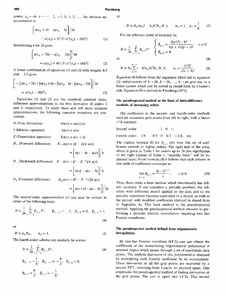
The explicit formula (8) for B,,, y tells how this set of coefficients extends to higher orders. The right half of the array above is given in Table 1 for orders up to 26 (the significance of the right column of Table 1, “stability limit,” will be ex- plained later). From formula (8) it follows that each column in this table of coefficients converges as

,(-,),+I lim B,, y = ~ v # 0. p-‘p v ’ (10)

Thus, there exists a limit method which theoretically has infinite accuracy. If one considers a periodic problem, the infi- nitely wide difference stencil applied to the data and to the periodic repetitions becomes equivalent to a stencil, as wide as the period, with modified coefficients (derived in closed form in Appendix A). This limit method is the pseudospectral method. Applying the pseudospectral method amounts to per- forming a periodic discrete convolution, requiring two fast Fourier transforms.

The pseudospectral method defined from trigonometric interpolation

By one fast Fourier transform (FFT), one can obtain the coefficients of the interpolating trigonometric polynomial of minimal degree which passes through a set of equidistant data points. The analytic derivative of this polynomial is obtained by multiplying each Fourier coefficient by its wavenumber. These derivatives at all the grid points are recovered by a second FFT, returning from Fourier to physical space. This constitutes the pseudospectral method of finding derivativesat the grid points. The cost is again two FFTs. This second

The Pseudospectral Method 485

definition is convenient for practical implementation since it explicitly gives the multipliers to use in Fourier space. The equivalent finite-difference coefficients are derived in Appendix A and are found to be identical to those derived from the limit of finite-difference methods.

COMPARISON OF THE PSEUDOSPECTRAL METHOD TO FINITE-DIFFERENCE METHODS OF DIFFERENT

ORDERS

Model equation to study dispersion

For elastic wave propagation in media with internal variations, the two phenomena which give the largest contri- butions to the final errors (exact versus numerical solution) are

(1) Dispersion (dissipation). Different Fourier modes, which should all travel with the same speed (no damping), in numerical schemes travel at different speeds (undergo damping). In particular, solutions with sharp gradients (e.g., step functions or short pulses) develop a wavetrain, most commonly trailing the pulse.

(2) Errors originating from variations in the medium. The simplest theory for the accuracy of numerical schemes requires the medium to be homogeneous. Rapid variations or sharp interfaces introduce complex interactions on incoming signals. Numerical schemes will typically suffer a loss in accuracy.

Dispersion can be studied fully with the simple model equation

au au -f-=0 at ax (11)

on the (periodic) interval --7[ 5 x < 1~. The centered schemes considered here are energy conserving (no dissipation). I present two different arguments regarding the effects of dispersive errors. In the first, equation (9) is used to determine different mode speeds and what errors they produce. In the second argument, I show that high-order methods are superior even in cases of nonsmooth solutions, for example, step functions. (Although local truncation errors are then large, small global errors result from cancellations.) This second point of view is crucial in understanding what generalizations (to nonlinear hyperbolic or parabolic equations, to boundary conditions of different kinds, etc.) the pseudospectral method can handle well and which it cannot.

The effect of solutions interacting with medium variations or discontinuities has not yet been analyzed satisfactorily. The few theoretical results available fail to predict the excellent results which emerge in test calculations such as the ones I present in Appendix B.

The pseudospectral method versus finite-difference methods for smooth solutions

Any (periodic) initial condition can be viewed as a superposition of Fourier modes. For the linear model [equation (1 i)], the modes can be studied individually. On a grid x, = x0 + vh, v = 0, 1, 2, . N - 1, the highest mode is eiomSXX, w,,, =

rr/h, h = 274N. (At the grid points, any higher mode becomes indistinguishable from a lower one within this range.) Consid- er a mode o, -a,,,,, I w I o,,, Then

whereas

DeiWX = i(t)$OX, (12)

D 0

@x -

eim(x+h) _ @u(x-h) sin oh _

2h = i h e’wx. (13)

Table 1. coefficients &V for difference approximations to d/dx.

order Of P Coefficients for difference approximations to d/dx

QtabilitY

ElCC”raCY limit

1 2 0.0 1.000

2 4 0.0 1.333 -0.167

3 6 0.0 1.500 -0.300

4 8 0.0 1.600 -0.400

5 10 0.0 1.667 -0.476

6 12 0.0 1.714 -0.536

1 14 0.0 1.750 -0.583

8 16 0.0 1.778 -0.622

3 18 0.0 1.800 -0.655

10 20 0.0 1.818 -0.682

11 22 0.0 1.833 -0.705

12 24 0.0 lA46 -0.725

13 26 0.0 1.857 -0.743

60 120 0.0 1.967 -0.936 0.574 -0.3134 0.264 -0.184 0.127 -0.087 0.058 -0.038 0.024 -0.015 0.009 . .

0.0 2.000 -1.000 0.667 -0.500 0.400 -0.333 0.286 -0.250 0.222 -0.200 0.182 -0.167 0.154 .

0.033

0.076

0.119

0.159

0.194

0.226

0.255

0.280

0.302

0.322

0.340

-0.007

-0.020

-0.036

-0.053

-0.071

-0.088

-0.105

-0.121

-0.136

-0.150

0.002

0.005

0.011

0.017

0.025

0.034

0.042

0.051

0.060

-0.000

-0.001

-0.003

-0.006

-0.009

-0.012

-0.017

-0.021

0.000

0.000 -0.000

0.001 -0.000 0.000

0.002 -0.000 0.000 -0.000

0.003 -0.001 0.000 -0.000 0.000

0.004 -0.001 0.000 -0.000 0.000 -0.000

0.006 -0.002 0.000 -0.000 0.000 -0.000 0.000

1.000

0.729

0.630

0.578

0.544

0.521

0.503

0.489

0.478

0.468

0.461

0.454

0.448

0.376

0.318

466 Fornberg

Omitting the imaginary unit i, the factors in front of eiox in the right-hand sides of equations (12) and (13) are displayed in Figure 1, together with the corresponding factors for the higher order difference methods. The convergence, for increasing orders, to the “ideal” line is slow. (It occurs in a way reminiscent of the convergence of a Taylor series; derivatives of successively higher orders match at the origin.)

For the model equation (1 l), dividing each factor by iw gives the speed by which the corresponding Fourier mode translates as time progresses. In the exact solution, all modes travel with speed 1. With second-order finite differences, higher modes move more slowly, up to the highest one (with values 1, - 1, 1, - 1, 1, at consecutive grid points), which does not travel at all.

A Fourier mode gives exactly the opposite contribution to what it should if its phase has drifted off by an angle of n. For the following analysis, I consider a mode to be accurate if its phase error is less than n/4. Then the number of modes (equal to the number of grid points) required when using different methods in space can be compared. I have chosen to consider the evolution over the time it takes a wave to travel once across the grid, i.e., over a time of 2rc. Note that this time is short in seismic applications where signals typically should have time to travel from the surface to the bottom and back again. The longer the time the more advantageous are the higher order (and the pseudospectral) methods (Kreiss and Oliger, 1972).

Figure 1 shows how to read the phase error for each frequency component at the final time Thus, for the second- order method, the requirement becomes

27c(D - Dg)eioX ieimx =+y)-f. (14)

For example, choosing a grid with N = 100 points (h = n/SO), equation (14) is satisfied if 1 w 1 < 5.76. Only 11.5 percent of the frequencies (ranging from - 50 to + 50 in this example) have kept their accuracy; 88.5 percent are lost by the dispersion.

’ Factor eiW’ Gets X/h -- Multiplled with

Phase Error of Mode at T=2n with 2nd Order FD:

2x w*- (

sin w’h

7)

FIG. 1. The factor the Fourier mode eiwx is multiplied by when different approximations to d/dx are applied (displayed as functions of the frequency w; a factor of l/i is omitted).

For the general method of order 2p, the corresponding in- equality follows from equation (9),

?n[w -y ~~~a,,Zi’(sin y)‘“] <t. (15)

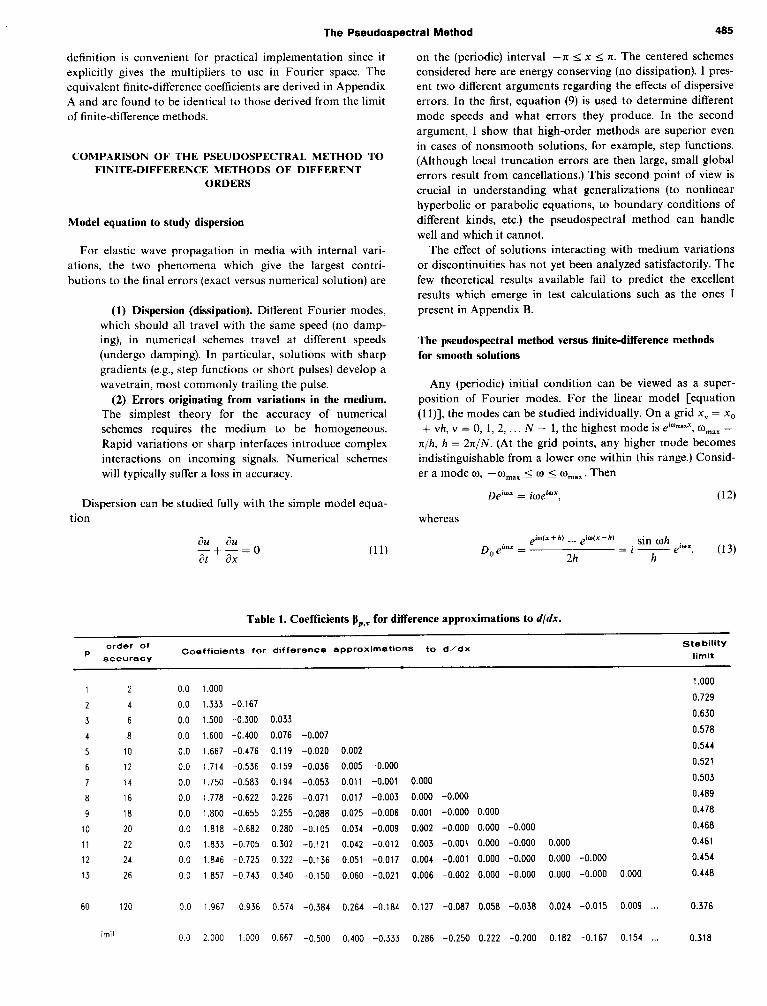
The relationships in Figures 2, 3, and 4 are calculated from equation (15). For various numbers of grid points N,, Figure 2 shows what proportion of all the modes on the grid gets lost. Figure 3 displays the same relationships in a different way. With N,V denoting the number of modes required to be accurate (phase error -C x/4) at the end, N, gives the number of grid points (equal to the total number of modes) required. In the range of N,V considered here, the relations shown in Figure 3 closely fit the formula

N, = cp N$+ li+), (16)

As an example of interpreting Figure 3, assume one wants to obtain a result with 32 correct modes. Following line 32 vertically until it intersects the lines for the pseudospectral method, fourth-. and second-order results shows that these methods would require approximately 32, 128, and 512 points, respectively (choosing the nearest power of two). In 2-D and 3-D applications, this argument applies in each direction.

Figure 4 displays the same relations, but relates them to wavelengths and points per wavelength. The horizontal scale differs by a factor of two from the horizontal scale in Figure 3. In the example above, 32-mode accuracy corresponds to 16 wavelengths across the grid. Following line 16 vertically until it intersects the lines for the different orders, one can find how many grid points are needed and alsc the corresponding number of points per wavelength.

The pseudospectral method versus finite-difference methods for step functions

Periodic, analytic initial data u(x) have Fourier repre- sentations with rapidly decreasing upper bounds for the coefficients: 1 f.?(w)) < c,e mc2~“‘~, This makes the Fourier analysis in

0 1 10 20 50 100 200 500 1000 NG

Number of grid points

FIG. 2. Proportion of Fourier modes which get lost due to dispersion.

_----- me--120th Order


the last section appropriate for comparing different methods. On the other extreme are functions whose variation is local and whose spectrum consequently is very wide. The spectrum of a step function has 1 C(w) 1 = 0(1/o) with derivative 1 C’(w) 1 = 0( 1). For a discrete delta function, these coefficients vary as 0( 1) and O(w), respectively. The Fourier expansions do not even converge as N + ~3. Very rough data are better viewed as a superposition of step functions than of Fourier modes. For this reason, it is of interest to analyze how the different methods treat a step solution.

The interpolation of a trigonometric polynomial to a discrete step function is subject to Gibbs phenomenon, an over- shoot of about 9 percent at each side of the jump. Oscillations die down only as 0(1/x) at a distance x from the jump. The pseudospectral method uses the derivative of this polynomial at the grid points, which will obviously lead to large errors even far from the jump. To obtain the derivative at a fixed time the pseudospectral method is not suitable. However, the present context is to solve equation (11) (or an equivalent equation) over a long time In the linear (or weakly nonlinear) hyperbolic case, the oscillatory errors cancel to give a very

high accuracy because the solution is largely translating across the grid.

A good way to measure the accuracy of a traveling step solution is to see how well it retains its slope over time Sup- pose 8,/5x in equation (11) is approximated by a difference operator D* of order 2p,

au t + D*v = 0. (17)

Then

t t analytic 2pth order in time in space

au au x + z + Ch2’

pp+ Iv dxz”+’ + 0(@+2) = 0. (18)

The evolution of the slope of a step (traveling along a line x = t + constant) is then, to leading order, approximated by the slope at x = 0 (t increasing) for the equation

+y + Ch2P a%+ lv

---co ax2p+l ’ (19)

NG

10 000

5000

2 000

1 000

3 .6 500 E s b z 200

b f 100

1

50

20

10

, -

, -

i * 10 20 50 100 200 500 1 000 N,

Number of modes required to meet the tolerapce 1 phase error 1 < ~14

FIG. 3. The number of grid points necessary with different methods as functions of the number of modes required to be accurate at final time

488

with initial conditions, for example,

v(x, 0) =

i

-% xto

0, x=0

% x>o

The solution to equations (19) and (20) is

“w I- u(x, t) = J 1 0 (cos chZPozp+‘t)(sin ox)

-Cc

+ (sin ~h*~ce*~+ ‘t)(cos wx) 1 do.

The derivative at x = 0 at time t becomes

au zxzo= -m I s m (cos ch*‘~~“+‘t) do = $@&.

Fornberg

(20)

(21)

(22)

The slope, infinite at t = 0, decays for increasing t as t’1(2p+11. For the slope to decay by a factor of two, time for a second- order method (p = 1) has to increase by a factor of eight. For a tenth-order method, the corresponding factor in time is over 2 000. The pseudospectral method is the limit for p+ CC.

40

35

30

c 5 4 25

g $ t 20 a (I) I a

15

10

5

2

A

I

Equation (22) suggests that the slope stays sharp forever, which is indeed the case. The pseudospectral method will “see” in the discrete data the interpolating trigonometric polynomial. All frequences in that polynomial, and hence in the whole polynomial, will translate exactly. The Gibbs phenomenon leads to a large local truncation error, but even so, there can be no growth of the error in time

Pseudospectral versus finite-difference methods for variable coefficients

The aim of this paper has been to provide an intuitive understanding. Accurate theory for the pseudospectral method in less ideal situations (e.g., for smoothly variable coefficients or for coefficients with jumps, even in 1-D situations) is rather incomplete. For finite-difference methods, the standard pro- cedure to get global error estimates is to add local truncation errors (which typically are small). In the pseudospectral method, on the other hand, local errors can be large (Gibbs phenomenon at a discontinuity is a typical case). Still, global errors grow very little with time due to cancellations. In some early literature on the pseudospectral method, this was not

. 2 5 10 20 50 100 200 500

Number of wavelengths withln computational Uomaln of highest wave mode which remains accurate at final die

FIG. 4. Number of grid points and number of points per wavelength required at different orders of finite differencing.


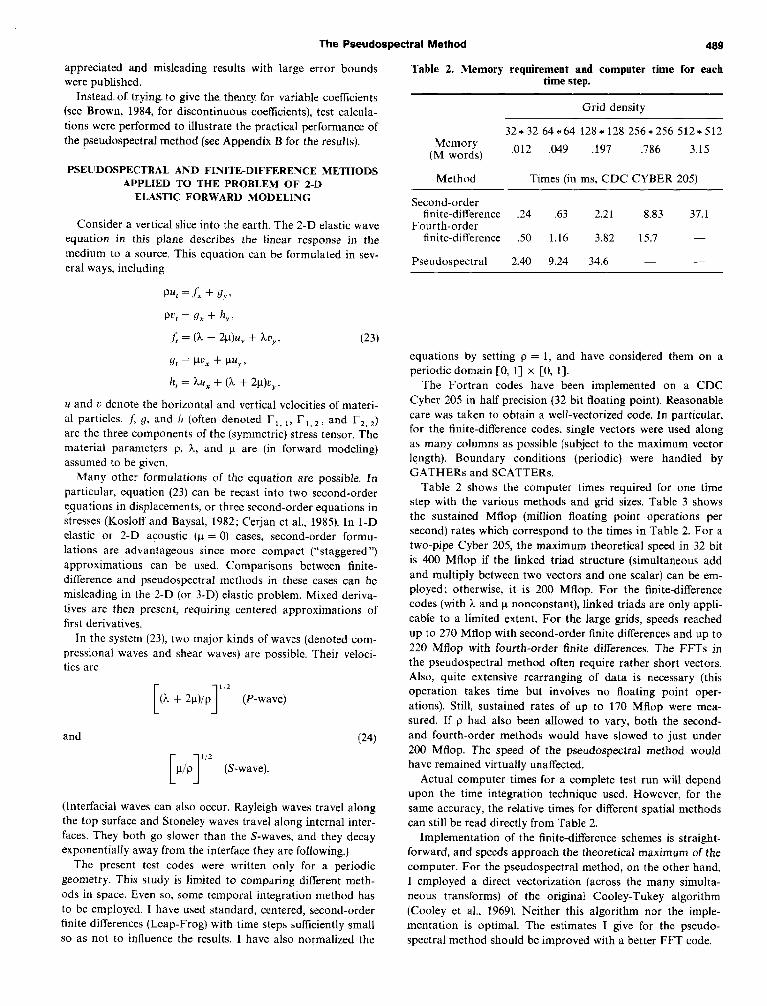
appreciated and misleading results with large error bounds Table 2. Memory requirement and computer time for each were published. time step.

Instead~ of trying to give the theor_y for_ variable coefficients (see Brown, 1984, for discontinuous coefficients), test calculations were performed to illustrate the practical performance of the pseudospectral method (see Appendix B for the results).

Ghd density

Memory (M words)

32*32 64*64 128*128 256*256 512*512

PSEUDOSPECTRAL AND FINITE-DIFFERENCE METHODS APPLIED TO THE PROBLEM OF 2-D

ELASTIC FORWARD MODELING

,012 ,049 ,197 .786 3.15

Consider a vertical slice into the earth. The 2-D elastic wave equation in this plane describes the linear response in the medium to a source. This equation can be formulated in several ways, including

Method Times (in ms, CDC CYBER 205)

Second-order finite-difference .24 .63 2.21 8.83 37.1

Fourth-order finite-difference .50 1.16 3.82 15.7

Pseudospectral 2.40 9.24 34.6 -

PU, =f, + gpr

Pa,=gr+h,,

f, = (h + 2u)u, + hn,, (23)

9, = W, + W,, , equations by setting p = 1, and have considered them on a periodic domain [0, l] x [0, 11.

h, = hu, + (h + 2u)n,.

u and u denote the horizontal and vertical velocities of material particles. J g, and h (often denoted l-i, 1, r1 2, and l-a J are the three components of the (symmetric) stre$s tensor. The material parameters p, h, and P are (in forward modeling) assumed to be given.

Many other formulations of the equation are possible. In particular, equation (23) can be recast into two second-order equations in displacements, or three second-order equations in siresses (Kosloff and Baysal, 1982; Cerjan et al., 1985). In 1-D elastic or 2-D acoustic (P = 0) cases, second-order formulations are advantageous since more compact (“staggered”) approximations can be used. Comparisons between finite- difference and pseudospectral methods in these cases can be misleading in the 2-D (or 3-D) elastic problem. Mixed derivatives are then present, requiring centered approximations of first derivatives.

The Fortran codes have been implemented on a CDC Cyber 205 in half precision (32 bit floating point). Reasonable care was taken to obtain a well-vectorized code. In particular, for the finite-difference codes, single vectors were used along as many columns as possible [subject to the maximum vector length). Boundary conditions (periodic) were handled by GATHERS and SCATTERS.

In the system (23), two major kinds of waves (denoted com- pressional waves and shear waves) are possible. Their velocities are

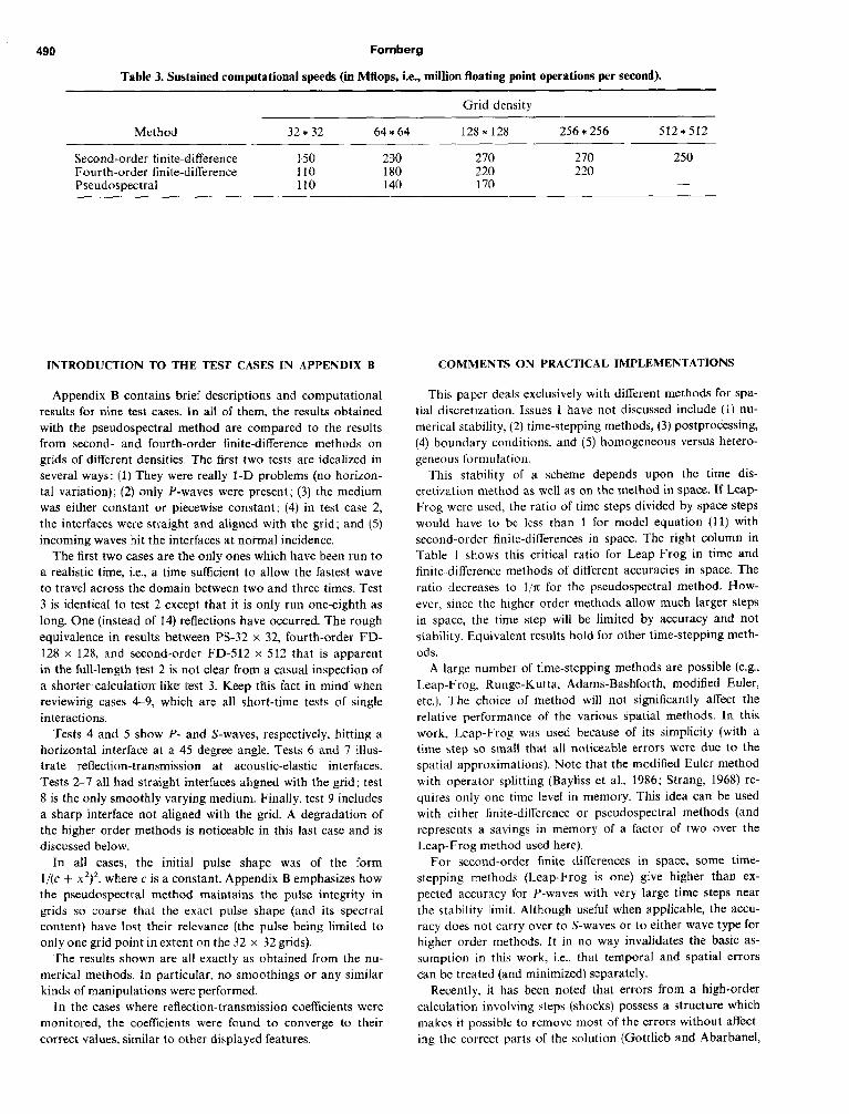
Table 2 shows the computer times required for one timestep with the various methods and grid sizes. Table 3 shows the sustained Mflop (million floating point operations per second) rates which correspond to the times in Table 2. For a two-pipe Cyber 205, the maximum theoretical speed in 32 bit is 400 Mflop if the linked triad structure (simultaneous add and multiply between two vectors and one scalar) can be employed; otherwise, it is 200 Mflop. For the finite-difference codes (with X and u nonconstant), linked triads are only applicable to a limited extent. For the large grids, speeds reached up to 270 Mflop with second-order finite differences and up to 220 Mflop with fourth-order finite differences. The FFTs in the pseudospectral method often require rather short vectors. Also, quite extensive rearranging of data is necessary (this operation takes time but involves no floating point operations). Still, sustained rates of up to 170 Mflop were measured. If p had also been allowed to vary, both the second- and fourth-order methods would have slowed to just under 200 Mflop. The speed of the pseudospectral method would have remained virtually unaffected.

[(X + 2u)/p]rii (P-wave)

and (24)

I 1 112

PIP (S-wave).

(Interfacial waves can also occur. Rayleigh waves travel along the top surface and Stoneley waves travel along internal interfaces. They both go slower than the S-waves, and they decay exponentially away from the interface they are following.)

The present test codes were written only for a periodic geometry. This study is limited to comparing different methods in space. Even so, some temporal integration method has to be employed. I have used standard, centered, second-order finite differences (Leap-Frog) with time steps sufficiently small so as not to influence the results. I have also normalized the

Actual computer times for a complete test run will depend upon the time integration technique used. However, for the same accuracy, the relative times for different spatial methods can still be read directly from Table 2.

Implementation of the finite-difference schemes is straight- forward, and speeds approach the theoretical maximum of the computer. For the pseudospectral method, on the other hand, I employed a direct vectorization (across the many simultaneous transforms) of the original Cooley-Tukey algorithm (Cooley et al., 1969). Neither this algorithm nor the implementation is optimal. The estimates I give for the pseudospectral method should be improved with a better FFT code.

490 Fornberg

Table 3. Sustained computational speeds (in Mflops, i.e., million floating point operations per second).

Grid density

Method 32~32 64~64 128 * 128 256 * 256 512*512

Second-nrder finite-difference 150 230 270 270 250 Fourth-order finite-difference 110 180 220 220 Pseudosnectral 110 140 170

INTRODUCTION TO THE TEST CASES 1N APPENDIX B COMMENTS ON PRACTICAL IMPLEMENTATIONS

Appendix B contains brief descriptions and computational results for nine test cases. In all of them, the results obtained with the pseudospectral method are compared to the results from second- and fourth-order finite-difference methods on grids of different densities. The first two tests are idealized in several ways: (1) They were really 1-D problems (no horizontal variation); (2) only P-waves were present; (3) the medium was either constant or piecewise constant; (4) in test case 2, the interfaces were straight and aligned with the grid; and (5) incoming waves hit the interfaces at normal incidence.

The first two cases are the only ones which have been run to a realistic time i.e., a time sufficient to allow the fastest wave to travel across the domain between two and three times. Test 3 is identical to test 2 except that it is only run one-eighth as long. One (instead of 14) reflections have occurred. The rough equivalence in results between PS-32 x 32, fourth-order FD- 128 x 128, and second-order FD-512 x 512 that is apparent in the full-length test 2 is not clear from a casual inspection of a shorter caiculaticm iike- testy 3. Keep this fact in minds when reviewing cases 4-9, which are all short-time tests of single interactions.

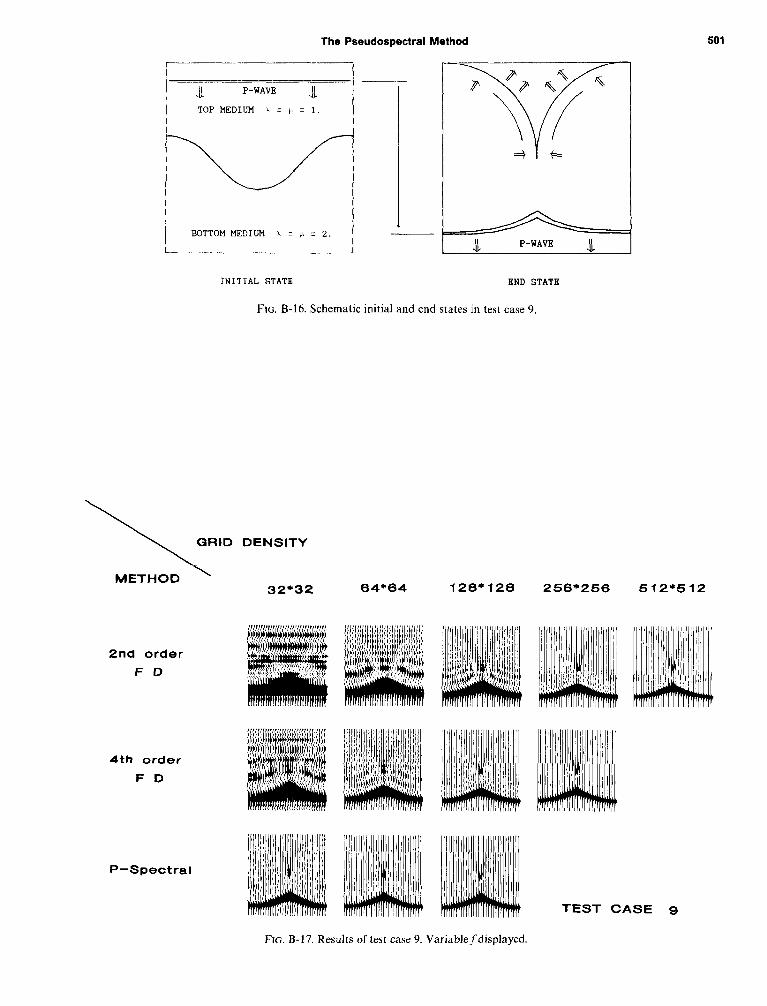
Tests 4 and 5 show P- and S-waves, respectively, hitting a horizontal interface at a 45 degree angle. Tests 6 and 7 illustrate reflection-transmission at acoustic-elastic interfaces. Tests 2-7 all had straight interfaces aligned with the grid; test 8 is the only smoothly varying medium. Finally, test 9 includes a sharp interface not aligned with the grid. A degradation of the higher order methods is noticeable in this last case and is discussed below.

In all cases, the initial pulse shape was of the form l/(c + x2)*, where c is a constant. Appendix B emphasizes how the pseudospectral method maintains the pulse integrity in grids so coarse that the exact pulse shape (and its spectral content) have lost their relevance (the pulse being limited to only one grid point in extent on the 32 x 32 grids).

The results shown are all exactly as obtained from the numerical methods. In particular, no smoothings or any similar kinds of manipulations were performed.

In the cases where reflection-transmission coefficients were monitored, the coefficients were found to converge to their correct values, similar to other displayed features.

This paper deals exclusively with different methods for spatial discretization. Issues 1 have not discussed include (1) numerical stability, (2) time-stepping methods, (3) postprocessing, (4) boundary conditions, and (5) homogeneous versus heterogeneous formulation.

This stability of a scheme depends upon the time discretization method as well as on the method in space. If Leap- Frog were used, the ratio of time steps divided by space steps would have to be less than 1 for model equation (11) with second-order finite-differences in space. The right column in Table 1 shows this critical ratio for Leap-Frog in time and finite-difference methods of different accuracies in space. The ratio decreases to l/n for the pseudospectral method. How- ever, since the higher order methods allow much larger steps in space, the time step will be limited by accuracy and not stability. Equivalent results hold for other time-stepping methods.

A large number of time-stepping methods are possible (e.g., Leap-Frog, Runge-Kutta, Adams-Bashforth, modified Euler, etc.). The choice of method will not significantly affect the relative performance of the various spatial methods. In this work, Leap-Frog was used because of its simplicity (with a time step so small that all noticeable errors were due to the spatial approximations). Note that the modified Euler method with operator splitting (Bayliss et al., 1986; Strang, 1968) requires only one time level in memory. This idea can be used with either finite-difference or pseudospectral methods (and represents a savings in memory of a factor of two over the Leap-Frog method used here).

For second-order finite differences in space, some time- stepping methods (Leap-Frog is one) give higher than ex- pected accuracy for P-waves with very large time steps near the stability limit. Although useful when applicable, the accuracy does not carry over to S-waves or to either wave type for higher order methods. It in no way invalidates the basic as- sumption in this work, i.e., that temporal and spatial errors can be treated (and minimized) separately.

Recently. it has been noted that errors from a high-order calculation involving steps (shocks) possess a structure which makes it possible to remove most of the errors without affect- ing the correct parts of the solution (Gottlieb and Abarbanel,


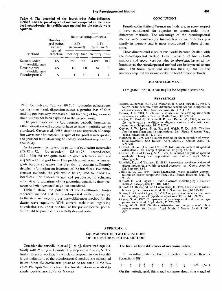
Table 4. The potential of the fourth-order finite-difference method and the pseudospectral method compared to the standard second-order finite-difference method for the elastic wave equation.

Relative computer costs Number of grid points 2-D 3-D

in each (measured) (estimated) spatial

Method direction memory time memory time-~-

Second-order 16N 256 20 4 096 300 finite-difference

Fourth-order 4N 16 1.8 64 8 finite-difference

Pseudospectral N 1 1 1 1

ACKNOWLEDGMENT

I am grateful to Dr. Alvin Bayliss for helpful discussions.

CONCLUSIONS

Fourth-order finite-difference methods are, in every respect I have considered, far superior to second-order finite- difference methods. The advantage of the pseudospectral method over fourth-order finite-difference methods lies primarily in memory and is most pronounced in three dimensions.

Three-dimensional calculations could become feasible with the pseudospectral method. Even if a factor of two in both memory and speed were lost due to absorbing layers at the ‘bourr&ari~, the pseudospectral method can be~expeeted to XR about 150 times faster and use less than l/2 000 of the memory required by second-order finite-difference methods.

1985; Gottlieb and Tadmor, 1985). In low-order calculations, on the other hand, dispersion causes a genuine loss of data, making postrecovery impossible. This favoring of higher order methods has not been exploited in the present work.

The pseudospectral method requires periodic boundaries. Other situations will somehow have to have a periodic setting simulated. Cerjan et al. (1985) describe one approach of damping waves near boundaries. In spite of the good results quoted, the problem with absorbing boundary conditions requires fur- ther study.

In the present test cases, the pattern of equivalent accuracies (PS-32 x 32; fourth-order, 128 x 128; second-order, 512 x 512) did not quite hold up when interfaces were not aligned with the grid lines. This problem will occur whenever grids become so sparse that they do not contain sufficiently detailed information on locations of the interfaces. For finite- element methods, the grid would be adjusted to follow the interfaces. For finite-difference and pseudospectral schemes, alternative formulations of the governing equations (homogeneous or heterogeneous) might be considered.

Table 4 shows the potential of the fourth-order finite- difference method and the pseudospectral method compared to the standard second-order finite-differences method for the elastic wave equation. With current techniques regarding boundaries, etc., about one-half of the pseudospectral potential should be possible in a carefully devised code.

REFERENCES

Bayliss, A., Jordan, K. E., Le Mesurier, B. J., and Turkel, E., 1986, A fourth order accurate finite difference scheme for the computation of elastic waves: Bull., Seis. Sot. Am., 76, 1115-I 132.

Brown, D. L., 1984, A note on the solution of the wave equation with piecewise smooth coefficients: Math Comp., 42, 369-391.

Cerjan, C., Kosloff, D., Kosloff, R., and Reshef, M., 1985. A nonre- fleeting boundary condition for discrete acoustic and elastic wave equations: Geophysics, 50, 705-708.

Cooley, J. W., Lewis, P. A. W., and Welch, P. D., 1969, The fast Fourier transform and its applications: Inst. Electr. Electron. Eng., Trans. Education, E-12, 27-34.

Fornberg, B., 1975, On a Fourier method for the integration of hyperbolic equations: Sot. Industr. Appl. Math., J. Numer. Anal., 12, 509-528.

Gottlieb, D., and Abarbanel, S., 1985, Information content in spectral calculations: Inst. Comp. Appl. in Sci. Eng. rep. 85-14.

Gottlieb, D., and Orszag, S. A., 1977, Numerical analysis of spectral methods. Theory and application: Sot. Industr. Appl. Math. Monograph.

Gottlieb, D., and Tadmor, E., 1985, Recovering pointwise values of discontinuous data within spectral accuracy: Inst. Comp. Appl. in Sci. Eng. rep. 85-3.

Johnson, 0. G., 1984, Three-dimensional wave equation compu- tations on vector computers: Proc., Inst. Electr. Electron. Eng., 72, 9G-95.

Kosloff, D., and Baysal, E., 1982, Forward modeling by a Fourier method: Geophysics, 47, 1402-1412.

Kosloff, D., Reshef, M., and Loewenthal, D., 1984, Elastic wave calculations by the Fourier method: Bull., Seis. Sot. Am., 74, 875-891.

Kreiss, H.-O., and Oliger, J., 1972, Comparison of accurate methods for the integration ofhvoerbolic equations: Tellus, 24, 199-215.

Orszag, S. A.: 1972, Comparison of pseudospectral and spectral approximation: Stud. Appl. Math., 51,253%259.

Strang, W. G., 1968, On the construction and comparison of difference schemes: Sot. Industr. Appl. Math., J. Numer. Anal., 5, 506 517.

APPENDIX A

EQUIVALENCE OF TWO DEFINITIONS OF THE PSEUDOSPECTRAL METHOD

Consider the periodic interval c--71, n], discretized equidis- tantly with N = 2p + 1 points. The step size is h = 2n/N. The

The limit of finite differences of increasing orders

finite-difference coefficients which correspond to the two dif- On an infinite interval, the limit method has the coefficients ferent definitions of the pseudospectral method are calculated [equation (IO)] below. Since the coefficients prove to be the same in the two 1... cases, the equivalence between the two definitions is verified (a \ I _$ f 4 -I 0 + _$ $ -2 .}/2J,, (A-1)

similar equivalence holds for N even). On the periodic grid, this stencil collapses down to a stencil of

492

width N = 2p + 1 with coefficients

{Y-P.P .” Y-l., Y0.a Yl,,

where

Y “,p=(_l)y+l f 2(-

k=-a, Nk+v

Yo,p = 0

and

Y y, P = -Y-V.p

Ye, ,P> (A-2)

Fornberg

The derivative at x = vh becomes

o<vsp,

(A-3)

--p<v<o.

To evaluate y,, p in closed form, consider the following integral over a rectangle with corners --M - (l/2) - iM, M + (l/2) - iA4, M + (l/2) + iM, -M -(l/2) + iM, where M (an integer) tends to infinity :

o=

2x

. N sin (xv/N) (A-4)

t t

Therefore,

Sum of residues at the poles of

x/sin (xz)

Residue at the pole z = -v/N

2x( - l)“+ ’ YV, p =

N sin (w/N) --plVSP, V#O

(A-5) Yo. p = 0.

Difference scheme corresponding to Fourier

interpolation

Consider a function,f(kh), k = --p, . . , p, defined at the grid points. The interpolating trigonometric polynomial is

f(X) = f: /(o)e’““, (‘4-6)

where

o= -p

{(CD) = $- i f(kh)e-ihk”. k- I,

(A-7)

f’(vh) = i i wf(cO)eio”*

P

= ; C f(kh) i c,xioh’“- k). (A-8) k- P w=-P

The corresponding finite-difference scheme over the N = 2p + 1 points therefore has the coefficients

IS-,., ... S-l,,, 6,,, F,,, ... S,,,I/2h, (A-9)

where

(A-10)

To evaluate 6,. p in closed form, note that for x # 0,

P i c f3K’“” = 2(sin x/2)*

(A-11) o= -p

Substituting x = hv = 2rrv/N gives, for v # 0,

h,, = -2 z{psin[(p+1)2xv/N] N’(sin rcv/N)

-(p + 1) sin (2xpv/N) (A-12)

The expression inside the braces simplifies as follows:

- sin 2pnvlN

(- l),+ ’ sin W/N

l-1)’

= (- 1)‘N sin xv/N. (A-13)

Therefore,

271( - l)“+ 1

- N sin (xv/N)

0.

~Psv<p,v#o

(A-14)

Thus the two ways to introduce the pseudospectral method are equivalent.


APPENDIX B

COMPARISONS BETWEEN SECOND- AND FOURTH-ORDER FINITE-DIFFERENCE METHODS AND THE PSEUDOSPECTRAL

METHOD IN NINE TEST CASES

Test case i-: Komogeneous medium @ = p = i-j.

Figure B-l shows schematically the initial and the end states in this test. A P-wave pulse has traveled 24 periods down. Figure B-2 compares the numerical solutions (snap- shots over space at the final time) for the different methods and different grid densities.

Test cases 2 and 3: Reflections at horizontal interfaces.

The medium has two horizontal interfaces, one at the center and (because of periodicity) one at the top (or bottom). Figure B-3 schematically shows the initial cases and the end case in test 2. P-wave trajectories for both cases are shown in Figure B-4. P-waves hit interfaces 14 times in case 2, once in case 3. Results of the two test cases are shown in Figures B-5 and B-6.

Test case 4: P-wave hitting an interface at 45 degrees.

Figure B-7 schematically shows the initial and end states in this test. The actual runs were performed in a periodic square of double the size shown. In the display of the results (Figure B-8), “grid density” refers to the grid size within the central square.

Test case 5: Swave hitting an interface at 45 degrees.

Figure B-9 schematically shows the inital and end states. In this case, there is no reflected P-wave. The domain was ex- tended as in case 4. The computational time was increased by a factor of 3”’ (to compensate for the slower S-wave speed). This has caused disturbances from the left edge of the bottom medium time to penetrate to the interior of the displayed square. These disturbances are visible in Figure B-10, in particular as an arc between the transmitted and reflected S- waves (i.e., they do not represent a flaw in any of the numerical schemes).

Test cases 6 at& 7 tm &waves hitting acoustic-elastics and elastic-acoustic interfaces at 45 degrees.

In test case 6 the schematic initial and end states are the same as in Figure B-7, except that the top medium is acoustic (h = 3, p = 0) instead of elastic (h = p = 1) and the reflected S-wave is missing. In test case 7, the bottom medium is changed from elastic (I. = p = .5) to acoustic (h = 3/2, p = 0). Again, the directions of all outgoing waves remain the same; however, the transmitted S-wave is now missing. Figure B-11 shows the same variable u at the end time for accurate solutions of the problems in three test cases 4, 6, and 7. This illustrates how the transmission-reflection coefficients differ. Results of the test cases 6 and 7 are given in Figures B-12 and B-13.

Test case 8: Smoothly varying medium; focusing of the wave.

The medium parameters (on the unit square) are

h = p = 1 - .5 exp (x - l/2)’ + (y - l/2)’ II . (B-l)

Contour curves are shown in Figure B-14 together with the scb~ernatic initial an& en-& &-atcs Tire slower bpmrh- of ihr signal near the center cause the incoming wave to focus and display a cusp-shaped front at the final time Results are shown in Figure B-l 5.

Test case 9: P-wave hitting a curved interface; focusing of both reflected and transmitted waves.

Figure B-16 shows schematic initial and end states. The computational time was chosen to bring the reflected P-wave exactly to its focus. Results are shown in Figure B-17.

Fornberg

METHOD _

INITIAL STATE

2nd order

FD

4th order

FD

P-Spectral

END STATE

FIG. B-l. Schematic initial and end states in test case 1.

DENSITY

32*32 64*64 128*128 256-256 512*512

TEST CASE 1

FIG. B-2. Results of test case 1. Variable u displayed.


BOTTOM MEDIUM X = p = .25

INITIAL STATE

lr P-WAVES lr

L L

t P-WAVES R

L L

t P-WAVES 'lk

L JL

END STATE IN TEST CASE 2

FIG. B-3. Schematic initial states in test cases 2 and 3 and end state in test case 2.

\

GRID DENSITY

METHOD

2nd order

FD

4th order

FD

32*32 64*64

(PERIODIC) TOP BOUNDARY

-_ -.-- NITIAL @\ FINAL time IN (PERIODIC) BOTTOM FINAL TIME IP time \ TEST CASE 3 BOUNDARY CONDITION TEST CASE 2

‘1 => time -

FIG. B-4. P-wave trajectories in test cases 2 and 3.

128*128 256-256 512+512

TEST CASE 2


2nd order

FD

4th order

FD

P-Spectrai

496 Fornberg

GRID DENSITY

METHOD 32*32 64*64 128*128 256+256 512*512

TEST CASE 3


TOP MEDIUM k = p = 1.

1 BOTTOM MEDIUM k q p = .5 ~--

INITIAL STATE END STATE

FIG. B-7. Schematic initial and end states in test case 4.

METHOD

2nd order

FD

4th order

FD

The Pseudospectral Method

DENSITY

32*32 64*64 128*128 256-256

P--Spectral

TEST CASE 4

FIG. B-8. Results of test case 4. Variable g displayed.

-.-___

BOTTOM MEDIUM \ = iI c .5 I

497



498 Fornberg

2nd order

FD

4th order

FD

P-Spectral

DENSITY

32-32 64.64 128&128 256*256

TEST CASE 5

FIG. B- 10. Results of test case 5. Variable u displayed.

TEST CASE 4:

ELASTIC OVER ELASTIC

TEST CASE 6:

ACOUSTIC OVER ELASTIC ____

TEST CASE 7:

ELASTlC OVER ACOUSTIC

FIG. B-l 1. Accurate pictures of the variable u at the end time in test cases 4,6, and 7.

2nd order

FD

4th order

FD

P-Spectral

The Pseudospectral Method

DENSITY

32*32 64*64 128*128 256*256

TEST CASE 6

METHOD

2nd order

FD

4th order

FD

P-Spectral


DENSITY

32-32 64*64 128-128 256-256


500 Fornberg

INITIAL STATE

I

END STATE

FIG. B-14. Contour curves for the variable medium and schematic initial and end states in test case 8.

GRID DENSITY

METHOD 32*32 64*64 128&128 256*256 512-512

2nd order

FD

4th order

FD

P-Spectral

TEST CASE 8

FIG. B-15. Results of test case 8. Variablefdisplayed.


_-_________ .l P-WAVE I

TOPMEDIUH \=11=1.

BOTTOM MEDIUM i = 1~ I 2.

i._.._____



\

GRID DENSITY

METHOD \

32*32 64+64 128*128 256+256 512’512

2nd order

FD

4th order

FD

P-Spectral

,I,,, TEST CASE Q

FIG. B-17. Results of test case 9. Variablefdisplayed.

Documents

The pseudospectral method: Comparisons with finite