Embed Size (px)
Citation preview
The Properties of Super Star Clusters in A Sample of
Starburst Galaxies
by
Kelsey Johnson
B.A., Carleton College, 1995
M.S., University of Colorado, 1997
A thesis submitted to the
Faculty of the Graduate School of the
University of Colorado in partial fulfillment
of the requirements for the degree of
Doctor of Philosophy
Department of Astrophysical and Planetary Sciences
2001
This thesis entitled:The Properties of Super Star Clusters in A Sample of Starburst Galaxies
written by Kelsey Johnsonhas been approved for the Department of Astrophysical and Planetary Sciences
Prof. Peter Conti
Prof. John Bally
Prof. Erica Ellingson
Prof. J. Michael Shull
Date
The final copy of this thesis has been examined by the signatories, and we find that both thecontent and the form meet acceptable presentation standards of scholarly work in the above
mentioned discipline.
iii
Johnson, Kelsey (Ph.D., Astrophysics)
The Properties of Super Star Clusters in A Sample of Starburst Galaxies
Thesis directed by Prof. Peter Conti
ABSTRACT
“Super star clusters” are the most massive extreme in the continuum of young star clus-
ters. In this thesis, I examine the properties of such super star clusters in a sample of starburst
galaxies with space and ground-based observations and in the optical, mid-infrared, and radio
regimes. Using optical photometry, I estimate the ages and masses, as well as construct luminos-
ity functions for the super star cluster systems. Additional H � observations allow me to place
tighter constraints on the burst ages and trace very recent star formation. The super star clusters
detected in these galaxies typically have estimated ages � ��� � Myr, masses of � � � � �� M , and
luminosity functions consistent with other super star cluster systems with a slope of ��� ���
( ��� ��������� ).Next I discuss an even earlier stage of massive star cluster evolution, when super star
clusters are still embedded in their birth material. I overview the discovery of “ultra dense H II
regions” (UDH IIs) with radio and mid-infrared observations. From the radio observations, I
calculate the electron densities, radii, and number of ionizing photons (and therefore number
of embedded massive stars). The mid-infrared observations confirm the presence of hot dust
cocoons surrounding these objects. These embedded clusters account for at least ��� � % of
the mid- to far-infrared flux of He 2-10. I also discuss the impact of UDH IIs on the radio to
far-infrared flux ratio.
Finally, I present a sample of 35 embedded star formation regions (ranging from the size
of small OB-associations to super star clusters) serendipitously detected in nearby galaxies.
This sample of objects begins to fill in the continuum of cluster masses between individual
UCH II regions and the embedded massive clusters.
iv
Acknowledgements
Perhaps the greatest irony of a thesis text is that the pages most likely to be read are those
of the acknowledgments. The weight of these pages is all the heavier because it is precisely the
people most likely to read them who most deserve to acknowledged, and I will undoubtedly
realize as soon as this thesis has been printed that several important people have been inadver-
tently left out. My sincere apologies in advance — to everyone who has provided me with kind
words, a welcome ear, new ideas, useful criticism, or their invaluable time, I am truly indebted.
A long, and sometimes complicated, path of people and events winds back through the
years which have brought me to this academic rite of passage. Most of these events were out
of my control, and most of these people I met by chance. The importance of serendipity has
not been lost on me, and I must acknowledge that I have been fantastically lucky. Here I will
roughly outline, in forward chronological order, the people who come to mind as having a large
impact on my academic career.
As an undergraduate at Carleton College, I was surrounded by caring faculty who didn’t
let me fall through the cracks – most importantly Dr. Cindy Blaha and Dr. Bruce Thomas. My
summer job working with Cindy was my springboard into the coming years. This summer job
in turn enabled me to work with Dr. Phil Massey in Arizona the following summer — again, a
lucky chance which has had a profound impact on my life since that time. Indeed, I have looked
to Phil for his infallible advice on both academic issues and those related to real life since that
summer. I believe that this work with Phil played a significant role in Dr. Peter Conti recruiting
me as a graduate student for the University of Colorado (although I don’t think either of them
v
would admit to this).
Peter has provided me with unwavering support during my time as a graduate student,
and perhaps most importantly has allowed me room to grow and explore new ideas (many of
which never came to fruition). I only hope that someday I have a fraction of his intuition and
patience. Along with Peter, Dr. Katy Garmany also had a large role in my academic advising
and went significantly beyond the “job description” many times. The unofficial title she held at
the University of Colorado of “Graduate Student Godmother” was certainly well deserved.
Upon arriving in graduate school, I briefly overlapped with Peter’s previous graduate
student, Dr. Margaret Hanson. Margaret is one of the most dynamic women I have had the
pleasure to know in astrophysics, and she has served as my primary role model through the
years. My officemate, Tanya Ramond, has also been an important part of my graduate life.
We have commiserated on many occasions, but have also shared many happy times. My office
sometimes seems like a second home, which hasn’t been so bad because I’ve had such a great
officemate.
Throughout my graduate student years I have also received a great deal of guidance from
afar — Dr. Bill Vacca has generously offered his time as a scientific advisor. He has been
exceedingly patient and I count him as one of the few people I am comfortable asking “stupid”
questions. As a measure of his conscientious replies to my queries, my email folder entitled
“Bill” has more entries than any other.
My work with Peter also led me to meet another valued collaborator and friend, Dr. Chip
Kobulnicky. With another nod to serendipity, it was my first interaction with Chip (I needed to
use one of his published images in a talk) which led us to discover “ultradense HII regions”.
These objects form a major part of this thesis and have led to numerous other opportunities for
which I am grateful.
Throughout graduate school I have been fortunate to have wonderful support structure
among the graduate students. I often question whether I would have survived my first two
years in the program without my classmates Sebastian Heinz, Aaron Lewis, and Kevin McLin.
vi
In particular, Kevin’s generosity stands out as I recall those years — on several occasions he
would do things like spontaneously bring me dinner when I didn’t have time to go home myself.
He also kept me from completely burying myself in work by coaxing me out for hikes in the
mountains. Along with my classmates, Marc DeRosa (DeRosa) and Marc Swisdak (Swisdak)
were a fundamental part of my support network. Because DeRosa had his office only a few
yards away from my own, he was often the recipient of random questions (both technical and
scientific). Swisdak was always willing to think through particularly vexing questions which I
wasn’t sure how to approach on my own. I greatly admire Swisdak’s character for his patience,
work ethic, fairness, and compassion, and hold his character up as a standard to which I aspire.
On a non-academic note, the Womprats and Nerfherders (the department’s intramural
ultimate teams), have provided an invaluable outlet for stress and a wonderful occasion to so-
cialize and get at least a little physical activity in my schedule. These teams even put up with
me as captain for several seasons, and it was a great pleasure to be a part of these teams as we
evolved from barely fielding a team of beginners to having over thirty players on two teams and
winning championships.
Finally, and most importantly, I come to my husband, Remy Indebetouw. Somehow he
stands by me when I am at my worst as well as celebrating with me when I am at my best. He
has kept me going on many occasions when I was ready to give up and has diligently protested
my complaints of not being smart enough, strong enough, or good enough. Throughout the
years we have been together, his influence on my life has helped me grow into a better person,
and his presence in my life gives me a sense of peace.
vii
Contents
Chapter
1 Introduction 1
1.1 Interpreting the Light From Stars . . . . . . . . . . . . . . . . . . . . . . . . 2
1.2 Starburst Galaxies . . . . . . . . . . . . . . . . . . . . . . . . . . . . . . . . 3
1.2.1 Relevance of Starburst Galaxies to the Early Universe . . . . . . . . . 4
1.2.2 Wolf-Rayet Galaxies . . . . . . . . . . . . . . . . . . . . . . . . . . . 6
1.2.3 What Causes a Starburst Episode? . . . . . . . . . . . . . . . . . . . . 7
1.3 Super Star Clusters . . . . . . . . . . . . . . . . . . . . . . . . . . . . . . . . 8
1.3.1 Where are Super Star Clusters Found? . . . . . . . . . . . . . . . . . 9
1.3.2 The Initial Mass Function and Cluster Mass Estimates . . . . . . . . . 10
1.3.3 The Luminosity Function of Super Star Clusters . . . . . . . . . . . . 13
1.3.4 Formation of Super Star Clusters . . . . . . . . . . . . . . . . . . . . . 14
1.4 The Birth Environment of Massive Star Clusters . . . . . . . . . . . . . . . . . 17
1.5 Thesis Outline . . . . . . . . . . . . . . . . . . . . . . . . . . . . . . . . . . . 18
2 The Case of Hickson Compact Group 31 20
2.1 Background . . . . . . . . . . . . . . . . . . . . . . . . . . . . . . . . . . . . 20
2.2 Observations and Data Reduction . . . . . . . . . . . . . . . . . . . . . . . . . 24
2.2.1 WFPC2 Data . . . . . . . . . . . . . . . . . . . . . . . . . . . . . . . 24
2.2.2 WIYN Data . . . . . . . . . . . . . . . . . . . . . . . . . . . . . . . . 30
viii
2.3 Results . . . . . . . . . . . . . . . . . . . . . . . . . . . . . . . . . . . . . . . 33
2.3.1 Optical Morphology . . . . . . . . . . . . . . . . . . . . . . . . . . . 33
2.3.2 Properties of the Super Star Clusters Compared to Models . . . . . . . 36
2.3.3 Luminosity Functions of the Super Star Clusters . . . . . . . . . . . . 45
2.3.4 Cluster Radii . . . . . . . . . . . . . . . . . . . . . . . . . . . . . . . 45
2.3.5 The Burst Luminosity . . . . . . . . . . . . . . . . . . . . . . . . . . 48
2.4 Discussion . . . . . . . . . . . . . . . . . . . . . . . . . . . . . . . . . . . . 52
2.4.1 The Star Formation History of HCG 31 . . . . . . . . . . . . . . . . . 52
2.4.2 On the Youth of Galaxy F . . . . . . . . . . . . . . . . . . . . . . . . 55
2.4.3 Globular Cluster Formation? . . . . . . . . . . . . . . . . . . . . . . . 56
2.4.4 Comparison to Other Starburst Systems . . . . . . . . . . . . . . . . . 58
3 The Case of Henize 2-10 60
3.1 Background . . . . . . . . . . . . . . . . . . . . . . . . . . . . . . . . . . . . 60
3.2 Observations and Data Reduction . . . . . . . . . . . . . . . . . . . . . . . . 61
3.3 Interpretation of Optical Images . . . . . . . . . . . . . . . . . . . . . . . . . 68
3.3.1 Optical Morphology . . . . . . . . . . . . . . . . . . . . . . . . . . . 68
3.3.2 The Burst Luminosity . . . . . . . . . . . . . . . . . . . . . . . . . . 72
3.3.3 Properties of the Super Star Clusters Compared to Models . . . . . . . 72
3.3.4 Luminosity Functions of the Super Star Clusters . . . . . . . . . . . . 78
3.3.5 Radii . . . . . . . . . . . . . . . . . . . . . . . . . . . . . . . . . . . 79
3.4 Discussion . . . . . . . . . . . . . . . . . . . . . . . . . . . . . . . . . . . . 79
3.4.1 On the Universality of SSC Luminosity Functions . . . . . . . . . . . 79
3.4.2 Comparison to Other Starburst Systems . . . . . . . . . . . . . . . . . 83
3.4.3 Implications of Large-Scale Outflow . . . . . . . . . . . . . . . . . . . 85
3.4.4 A Note of Caution . . . . . . . . . . . . . . . . . . . . . . . . . . . . 88
ix
4 The Discovery of “Ultradense HII Regions”:
The Early Stages of Massive Star Cluster Evolution 90
4.1 Background . . . . . . . . . . . . . . . . . . . . . . . . . . . . . . . . . . . . 90
4.2 Observations and Data Reduction . . . . . . . . . . . . . . . . . . . . . . . . . 91
4.2.1 VLA Radio Continuum Observations . . . . . . . . . . . . . . . . . . 91
4.2.2 Gemini Mid-Infrared Observations . . . . . . . . . . . . . . . . . . . . 92
4.3 Comparison of Optical, Radio, and Mid-IR Images . . . . . . . . . . . . . . . 96
4.4 The Nature of These Radio Sources . . . . . . . . . . . . . . . . . . . . . . . 97
4.4.1 Could These Objects be Supernovae Remnants? . . . . . . . . . . . . . 98
4.4.2 Could These Objects be AGN? . . . . . . . . . . . . . . . . . . . . . . 99
4.4.3 Could These Objects be Enshrouded H II Regions? . . . . . . . . . . . 99
4.5 Physical Properties of the Dense H II Regions . . . . . . . . . . . . . . . . . . 101
4.5.1 Emission Measures . . . . . . . . . . . . . . . . . . . . . . . . . . . . 101
4.5.2 Comparison With Model H II Regions . . . . . . . . . . . . . . . . . 104
4.5.3 Limits on the Contribution From SNe . . . . . . . . . . . . . . . . . . 104
4.5.4 Ionizing Radiation . . . . . . . . . . . . . . . . . . . . . . . . . . . . 105
4.5.5 Stellar Content . . . . . . . . . . . . . . . . . . . . . . . . . . . . . . 107
4.6 Discussion . . . . . . . . . . . . . . . . . . . . . . . . . . . . . . . . . . . . . 108
4.6.1 On the Lifetimes of UDH IIs . . . . . . . . . . . . . . . . . . . . . . 108
4.6.2 UDH IIs in Other Starburst Systems? . . . . . . . . . . . . . . . . . . 110
4.6.3 Implications for the Infrared-Radio Correlation? . . . . . . . . . . . . 113
5 A Sample of Clusters of Extragalactic Ultracompact H II Regions 116
5.1 Background . . . . . . . . . . . . . . . . . . . . . . . . . . . . . . . . . . . . 116
5.2 Galaxies in This Sample . . . . . . . . . . . . . . . . . . . . . . . . . . . . . 118
5.2.1 M33 . . . . . . . . . . . . . . . . . . . . . . . . . . . . . . . . . . . . 118
5.2.2 NGC 253 . . . . . . . . . . . . . . . . . . . . . . . . . . . . . . . . . 119
x
5.2.3 NGC 6946 . . . . . . . . . . . . . . . . . . . . . . . . . . . . . . . . 120
5.3 Results . . . . . . . . . . . . . . . . . . . . . . . . . . . . . . . . . . . . . . 121
5.3.1 Detection of UDH II Candidates . . . . . . . . . . . . . . . . . . . . . 121
5.3.2 Comparison to Optical Images . . . . . . . . . . . . . . . . . . . . . . 124
5.3.3 Modeled Properties . . . . . . . . . . . . . . . . . . . . . . . . . . . . 136
5.4 Discussion . . . . . . . . . . . . . . . . . . . . . . . . . . . . . . . . . . . . . 142
5.4.1 Stellar Content . . . . . . . . . . . . . . . . . . . . . . . . . . . . . . 142
5.4.2 Comparison to W49A . . . . . . . . . . . . . . . . . . . . . . . . . . 143
5.4.3 On the Youth of UDH II Regions . . . . . . . . . . . . . . . . . . . . . 149
6 Future Work 150
6.1 Expand the Sample of Known UDH IIs . . . . . . . . . . . . . . . . . . . . . 150
6.2 Determine the Properties of the Birth Environments of Massive Star Clusters . 151
6.3 Determine the Properties of Massive Star Clusters at Different Evolutionary
Stages . . . . . . . . . . . . . . . . . . . . . . . . . . . . . . . . . . . . . . . 153
6.4 Identify an Evolutionary Sequence . . . . . . . . . . . . . . . . . . . . . . . . 154
6.5 Develop More Sophisticated Models . . . . . . . . . . . . . . . . . . . . . . . 156
6.6 Summary of Future Possibilities . . . . . . . . . . . . . . . . . . . . . . . . . 156
Appendix
A UCH II Candidates in the Magellanic Clouds 169

Tables
Table
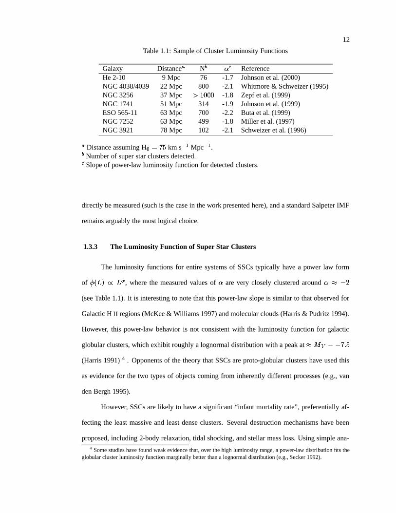
1.1 Sample of Cluster Luminosity Functions . . . . . . . . . . . . . . . . . . . . . 13
2.1 Completeness limits found in each of the four filters for NGC 1741 as described
in the text. . . . . . . . . . . . . . . . . . . . . . . . . . . . . . . . . . . . . . 27
3.1 Completeness limits found in each of the three filters as described in the text. . 66
4.1 Properties of Individual Radio Knots . . . . . . . . . . . . . . . . . . . . . . . 92
5.1 UDH II candidates in M33 . . . . . . . . . . . . . . . . . . . . . . . . . . . . 122
5.2 UDH II candidates in NGC 253 . . . . . . . . . . . . . . . . . . . . . . . . . 123
5.3 UDH II candidates in NGC 6946 . . . . . . . . . . . . . . . . . . . . . . . . . 125
5.4 Comparison with optical images of M33 . . . . . . . . . . . . . . . . . . . . . 125
5.5 Comparison with optical images of NGC 253 . . . . . . . . . . . . . . . . . . 126
5.6 Comparison with optical images of NGC 6946 . . . . . . . . . . . . . . . . . . 132
5.7 Estimated emission measures . . . . . . . . . . . . . . . . . . . . . . . . . . . 137
A.1 UCH II candidates in the LMC. . . . . . . . . . . . . . . . . . . . . . . . . . 172
A.1 continued. . . . . . . . . . . . . . . . . . . . . . . . . . . . . . . . . . . . . . 173
A.2 UCH II candidates in the SMC. . . . . . . . . . . . . . . . . . . . . . . . . . . 173
xii
Figures
Figure
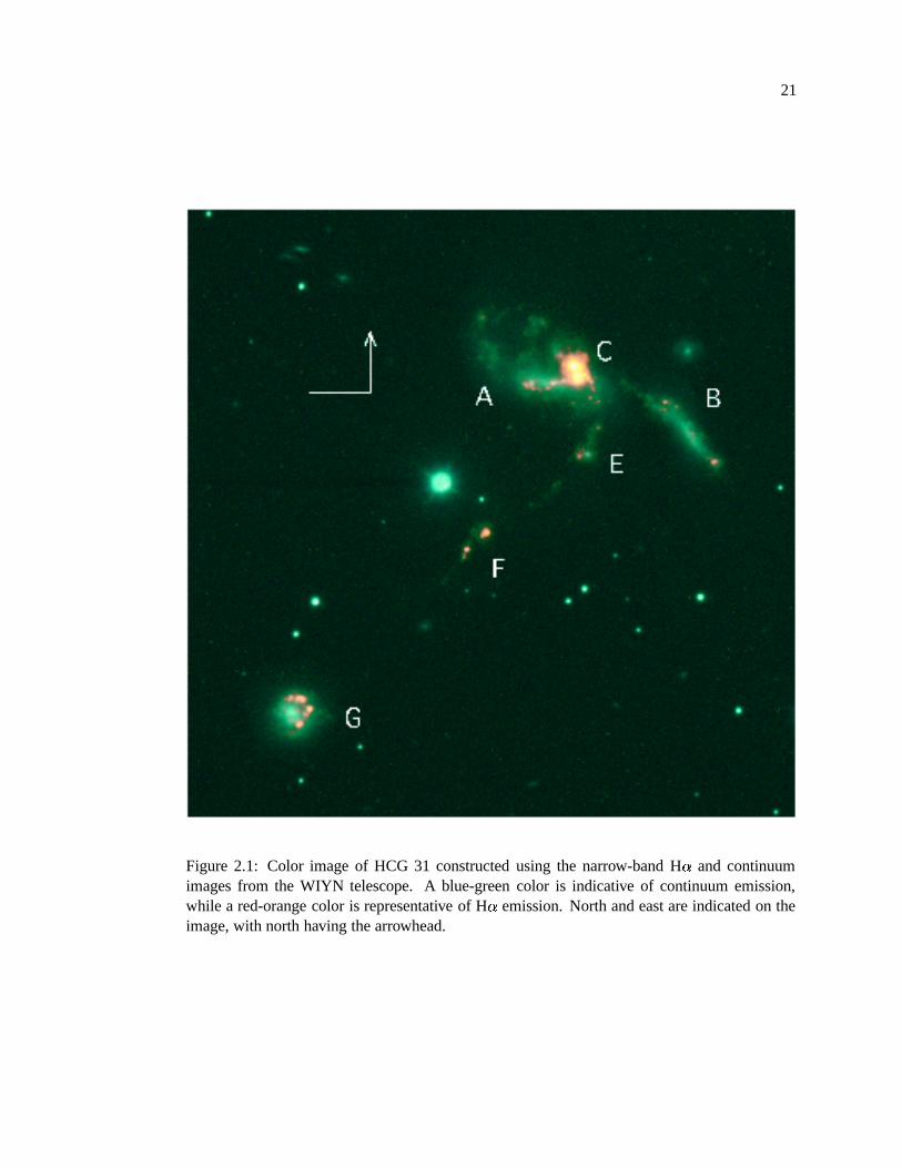
2.1 Color image of HCG 31 constructed using the narrow-band H � and continuum
images from the WIYN telescope. A blue-green color is indicative of contin-
uum emission, while a red-orange color is representative of H � emission. North
and east are indicated on the image, with north having the arrowhead. . . . . . 23
2.2 Uncertainties as a function of magnitude for the F439W, F555W, F675W, and
F814W filters. (top) galaxies A and C; (bottom) galaxies E and F. . . . . . . . 29
2.3 Color image of NGC 1741 constructed using the��� �
, � � � , and � � � images
from HST. The color scales have been enhanced to illustrate the differences in
color throughout the galaxy, however if true color were used the entire galaxy
would appear blue-white. . . . . . . . . . . . . . . . . . . . . . . . . . . . . 31
2.4 � � � images of (top) galaxy E and (bottom) galaxy F from HST. North and east
are indicated on the images, with north having the arrowhead. Both images are
shown at the same physical scale. . . . . . . . . . . . . . . . . . . . . . . . . 32
2.5 Uncertainties as a function of W(H � ) (in A) for the WIYN data. . . . . . . . . 34
2.6 Color-color plot for NGC 1741 in the HST magnitude system with a Vega ze-
ropoint. The model including only stellar light are shown with open circles,
and the model including stellar and nebular line emission is shown with filled
circles. . . . . . . . . . . . . . . . . . . . . . . . . . . . . . . . . . . . . . . 38
xiii
2.7 � � � vs � � � � � � � plot for the SSCs in HCG 31 (galaxy AC top, galaxies E
and F bottom). The burst models for both stellar light and nebular emission
are shown for masses of � � � � � � � � � � � � and � � � M , with the models for only
stellar light being shown with a dotted line. The youngest and oldest ages of the
models shown are 1 Myr and 10 Myr, respectively, with the younger ages being
bluer. . . . . . . . . . . . . . . . . . . . . . . . . . . . . . . . . . . . . . . . 39
2.8 Model predictions from Leitherer et al. (1999) for W(H � ) vs. age are shown
(top) along with a histogram of the W(H � ) values for SSCs in HCG31 (bottom). 43
2.9 A histogram of the W(H � ) values for SSCs in each of the member galaxies of
HCG31. Higher W(H � ) values correspond to younger ages. . . . . . . . . . . 44
2.10 The � luminosity function of the SSCs in NGC 1741 in the Johnson-Cousins
system. Magnitudes fainter than the completeness limit are shown with a dotted
line. For���
less than the completeness limit, the LF is well fit by a power law
of the form ��� ��� ��� �� . . . . . . . . . . . . . . . . . . . . . . . . . . . . . 46
2.11 The � � � � � � � histogram in the Johnson-Cousins system. No internal reddening
correction has been applied. . . . . . . . . . . . . . . . . . . . . . . . . . . . 47
2.12 The relation between the ��� � � � magnitudes and the effective radii for the � � �
filter. . . . . . . . . . . . . . . . . . . . . . . . . . . . . . . . . . . . . . . . 49
2.13 The radii estimated for the super star clusters in NGC 1741 in the � � � filters
using the method described in the text. Most of the sources are clearly unre-
solved. Although a few may be marginally resolved, they are consistent with
being point sources within the uncertainty. As shown in Figure 2.12, the method
used to estimate these radii is strongly degenerate for radii greater than approx-
imately 3 pc. . . . . . . . . . . . . . . . . . . . . . . . . . . . . . . . . . . . 50
2.14 The isophotal dependence of the � � � � � � � and� � � �� � � colors for the
integrated light from NGC 1741. It is clear that the derived colors of the galaxy
are dependent on the boundary used. . . . . . . . . . . . . . . . . . . . . . . 53
xiv
3.1 A multi-color image of He 2-10 constructed using the F555W, F814W, and
F658N images. F658N is shown in red, and therefore a blue-green color in the
image should be interpreted as continuum. The scale of this image is approxi-
mately 1.3 kpc on a side. . . . . . . . . . . . . . . . . . . . . . . . . . . . . . 63
3.2 Errors as a function of magnitude for the F555W and F814W filters. . . . . . . 65
3.3 A map of the W(H � ) in He 2-10, where the brighter colors correspond to larger
equivalent widths. North and east are indicated on the image, with north having
the arrowhead. This image is shown with the same scale and orientation as
Figure 3.1 — the length of the compass arms is approximately 100 pc. . . . . 67
3.4 A F555W image of He 2-10 with the GHRS apertures used in Johnson et al.
(2000) ( � � � � � ��� � � � � � � or approximately 75 pc�
75 pc) overlaid on starburst
regions A (west) and B (east). North and east are indicated on the image, with
north having the arrowhead. Note that this image has the same scale and orien-
tation as Figure 3.1 and Figure 3.3. . . . . . . . . . . . . . . . . . . . . . . . 70
3.5 The nuclear region of He 2-10 shown in F555W (left) and W(H � ) (right) where
brighter colors correspond to SSCs and stellar background in (a) and larger
equivalent widths in (b). These images are registered to each other and shown
in the same orientation as Figures 3.3 and 3.4, and are approximately 250 pc on
a side. . . . . . . . . . . . . . . . . . . . . . . . . . . . . . . . . . . . . . . . 71

xv
3.6 The � � � magnitude and � � � - � � � colors of the SSCs brighter than � � �
� ��� � � in He 2-10 along with the models including only stellar light (dashed
line) or including both stellar light and nebular line emission in blue (solid line).
(a) SSCs found in region A are shown as open circles, region B as triangles,
and the extension to the north-west of region A as filled circles. The ages are
labeled along the � � � M only, but the lower mass track behaves similarly.
No correction for internal reddening in He 2-10 has been applied, but a de-
reddening vector of A� � � is shown for reference. Typical uncertainties are
indicated in the upper right corner. (b) The SSCs detected in the F658N filter
are shown with W(H � ) � 100 as large circles and W(H � ) as small circles. . . 74
3.7 A histogram of the W(H � ) values for SSCs in He 2-10 is shown (bottom) along
with model predictions (top) from Leitherer et al. (1999) for W(H � ) vs. age. . 76
3.8 The locations of the SSCs detected in the F658N filter are shown. The plot has
the same dimensions and orientation as Figures 3.1, 3.3 and 3.4. An optical
contour is also shown for reference. Because of their larger W(H � ), the central
SSCs in region A must be younger than those in region B. . . . . . . . . . . . 77
3.9 The � � � luminosity function of the SSCs in He 2-10 shown with a solid line
brightward of the completeness limit. The power law fit brighter than � � �
� ��� � � is shown with a dashed line. No correction for internal reddening in
He 2-10 has been applied. . . . . . . . . . . . . . . . . . . . . . . . . . . . . 80
3.10 The � � � - � � � plot for the SSCs in He 2-10. No correction for internal redden-
ing in He 2-10 has been applied. . . . . . . . . . . . . . . . . . . . . . . . . . 81
3.11 A histogram of the radii measured using the ��� � �� magnitudes for the sources
in He 2-10. . . . . . . . . . . . . . . . . . . . . . . . . . . . . . . . . . . . . 82
xvi
4.1 HST WFPC2 F555W (V-band) image of He 2-10 in colorscale overlaid with
VLA B-array 2 cm radio continuum contours with a synthesized beam of � � � � � � �
� � � � � � FWHM. This image is approximately��� � � ���
�� � �
, and shown at the same
scale and orientation as Figure 4.2. It is clear that the 2 cm radio sources do not
correspond to the optical SSCs. . . . . . . . . . . . . . . . . . . . . . . . . . 94
4.2 Gemini N-band image of He 2-10 in colorscale overlaid with the same 2 cm
contours as Figure 4.1. At least three of the five radio sources are also strong
mid-IR sources. The mid-IR morphology is strongly correlated to the radio
morphology, but quite dissimilar from the optical morphology. . . . . . . . . . 95
4.3 VLA 6 cm and 2 cm fluxes for the five radio knots in He 2-10. Model spectral
energy distributions are shown for an ionized sphere of hydrogen with uniform
temperature and density. The radius and density used to model each source are
listed in the upper left corner. . . . . . . . . . . . . . . . . . . . . . . . . . . 102
4.4 The spectral energy distribution of the UDH IIs in He 2-10. The 12 � m, 25 � m,
60 � m, and 100 � m have been estimated by multiplying the total IRAS flux of
He 2-10 by the fractional percentage of the total N-band flux for each UDH II. 103
4.5 Best fit electron density and radius for the UDH II in NGC 5253 detected by
Turner et al. (2000). The models are the same as described in � 4.5.2 and use an
electron temperature of 11,000 K as derived by Kobulnicky et al. (1997). . . . 112
5.1 Locations of the detected UDH IIs in M33 are shown (along with their number
in Table 5.1) with respect to the B-band images (shown in gray scale). The
identification circles are � � � �in diameter, reflecting the beam size of the radio
observations. North is up and East is left. These images are all approximately
� � � � on a side. . . . . . . . . . . . . . . . . . . . . . . . . . . . . . . . . . . . 127
xvii
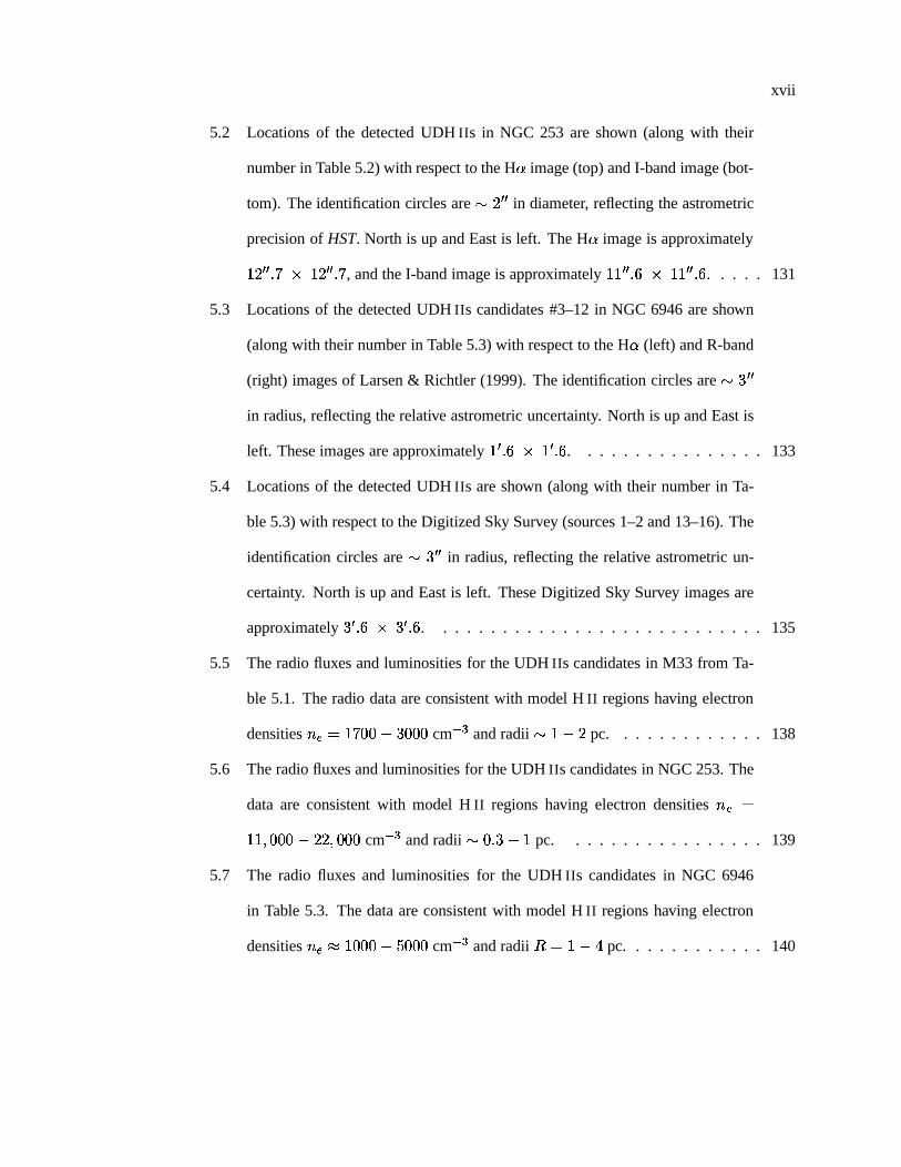
5.2 Locations of the detected UDH IIs in NGC 253 are shown (along with their
number in Table 5.2) with respect to the H � image (top) and I-band image (bot-
tom). The identification circles are � � � � in diameter, reflecting the astrometric
precision of HST. North is up and East is left. The H � image is approximately
� � � � � � � � � � � � � , and the I-band image is approximately � � � � � � � � � � � � � . . . . . 131
5.3 Locations of the detected UDH IIs candidates #3–12 in NGC 6946 are shown
(along with their number in Table 5.3) with respect to the H � (left) and R-band
(right) images of Larsen & Richtler (1999). The identification circles are � � � �
in radius, reflecting the relative astrometric uncertainty. North is up and East is
left. These images are approximately � � � � � � � � � . . . . . . . . . . . . . . . . 133
5.4 Locations of the detected UDH IIs are shown (along with their number in Ta-
ble 5.3) with respect to the Digitized Sky Survey (sources 1–2 and 13–16). The
identification circles are � � � � in radius, reflecting the relative astrometric un-
certainty. North is up and East is left. These Digitized Sky Survey images are
approximately� �� � ��� �
� � . . . . . . . . . . . . . . . . . . . . . . . . . . . . 135
5.5 The radio fluxes and luminosities for the UDH IIs candidates in M33 from Ta-
ble 5.1. The radio data are consistent with model H II regions having electron
densities ��� � � � � � � � � � � cm �� and radii � � � � pc. . . . . . . . . . . . . 138
5.6 The radio fluxes and luminosities for the UDH IIs candidates in NGC 253. The
data are consistent with model H II regions having electron densities ��� �
� � � � � � � � � � � � � cm � � and radii � � � � � � pc. . . . . . . . . . . . . . . . . 139
5.7 The radio fluxes and luminosities for the UDH IIs candidates in NGC 6946
in Table 5.3. The data are consistent with model H II regions having electron
densities ��� � � � � � � � � � � cm �� and radii � � � � pc. . . . . . . . . . . . 140
xviii
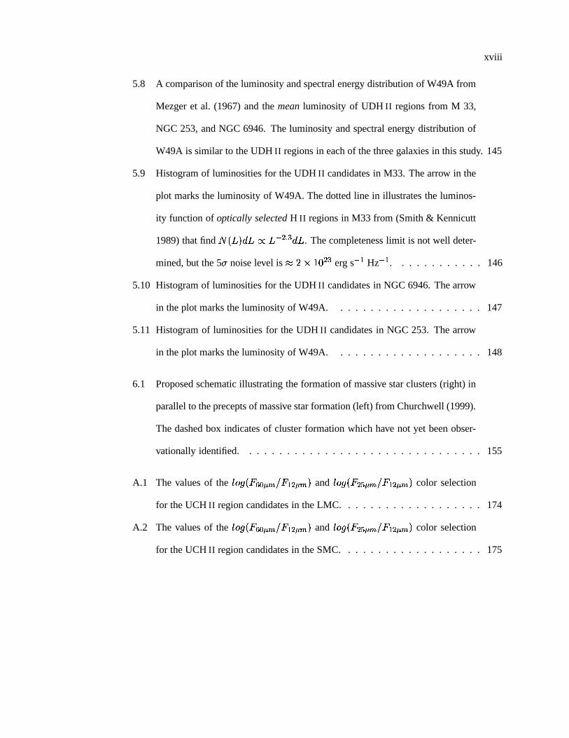
5.8 A comparison of the luminosity and spectral energy distribution of W49A from
Mezger et al. (1967) and the mean luminosity of UDH II regions from M 33,
NGC 253, and NGC 6946. The luminosity and spectral energy distribution of
W49A is similar to the UDH II regions in each of the three galaxies in this study. 145
5.9 Histogram of luminosities for the UDH II candidates in M33. The arrow in the
plot marks the luminosity of W49A. The dotted line in illustrates the luminos-
ity function of optically selected H II regions in M33 from (Smith & Kennicutt
1989) that find� � ��� � � ��� ��� � � � . The completeness limit is not well deter-
mined, but the 5 � noise level is ��� � � � � � erg s ��� Hz ��� . . . . . . . . . . . . 146
5.10 Histogram of luminosities for the UDH II candidates in NGC 6946. The arrow
in the plot marks the luminosity of W49A. . . . . . . . . . . . . . . . . . . . 147
5.11 Histogram of luminosities for the UDH II candidates in NGC 253. The arrow
in the plot marks the luminosity of W49A. . . . . . . . . . . . . . . . . . . . 148
6.1 Proposed schematic illustrating the formation of massive star clusters (right) in
parallel to the precepts of massive star formation (left) from Churchwell (1999).
The dashed box indicates of cluster formation which have not yet been obser-
vationally identified. . . . . . . . . . . . . . . . . . . . . . . . . . . . . . . . 155
A.1 The values of the � � � � � � �� � � � � � and � � � � � � �� � � � � � color selection
for the UCH II region candidates in the LMC. . . . . . . . . . . . . . . . . . . 174
A.2 The values of the � � � � � � �� � � � � � and � � � � � � �� � � � � � color selection
for the UCH II region candidates in the SMC. . . . . . . . . . . . . . . . . . . 175
Chapter 1
Introduction
“My purpose is to tell of bodies which have been transformed into shapes of a different kind.
You heavenly powers, since you were responsible for those changes, as for all else, look
favourably on my attempts, and spin an unbroken thread of verse, from the earliest beginnings
of the world, down to my own times.”
— Ovid (Metamorphoses)
The universe is host to a multitude of physical processes, and an equally diverse col-
lection of material elements, which are continually interacting and evolving. Throughout this
cosmic dance, generations of stars have been born, died, and created anew from the ashes. This
cycle of life continues even today in our own galaxy, the Milky Way. As we look further and
further into the depths of the universe, we see that stars have been forming almost since the
beginning of time. As their light crosses the vast expanse of time and space, it carries along
encrypted information that we have learned how to decode, and in this way have gained much
of our understanding of the universe.
Because this thesis is primarily based on observations, I will begin by providing a basic
explanation of how astronomers decode this light from the universe in � 1.1, which is included
for the benefit of readers outside of the field. In the remainder of this chapter, I will give a broad
overview of topics closely related to the subject of this thesis. The nature of starburst galaxies
and their impact throughout the universe is discussed in � 1.2. The state of knowledge about
super star clusters, which are typically formed in starburst episodes, is discussed in � 1.3.
2
1.1 Interpreting the Light From Stars
In nature’s endless variety, even stars themselves have a rich family of sub-types and
species — in fact, there is literally a rainbow of stellar types. One can think of fire as an
analogy, a flame is blue at its hottest and red where it is cool. Likewise, stars have a continuum
of colors, with the hottest being blue and the coolest red. For most of a star’s life (known as
the “main sequence”) 1 , its color not only tells us about its temperature, but also about its
most fundamental property, mass. The lives of stars are deterministic in this way — the mass
with which a star is born virtually dictates the rest of its life (with a few more subtle effects
intentionally neglected here). The most massive stars live fast and die young: the more massive
a star is, the faster it consumes its fuel and the brighter it burns. While our cool and yellow
Sun will live some 10 billion years, by contrast a hot blue star will die at the young age (by
astronomical standards) of only a few million years. For this reason, if we see a bright blue star
on the main sequence, we know it has to be young.
In this way, we can also use color to learn about collections of stars, such as galaxies.
Even if we cannot resolve the individual stars themselves, the medley of stellar light coming
from a galaxy tells us something about the stars it contains. Even more can be learned from
light if we spread it out into a rainbow or “spectrum”. Each type of star (and other astrophysical
objects as well) has a unique fingerprint which we can identify in its spectrum. These are the
main tools astronomers use to understand the universe with observations. For example, a galaxy
with an unusually blue color must have an abundance of blue stars 2 . Since these stars must
be young, the galaxy’s blue color indicates that it must have recently undergone a tremendous
spurt of star formation. These are the galaxies which we call “starbursts”.1 As a star nears the end of its life, it enters the “post main sequence”. During post main sequence evolution, a
star’s color does not directly reflect its mass.2 A reader familiar with the field will note that I am neglecting the class of starburst galaxies which are luminous
in the infrared due to tremendous amounts of dust which reprocesses the light from the hot blue stars.
3
1.2 Starburst Galaxies
It has been over 30 years since Sargent & Searle (1970) noted that certain galaxies are
undergoing intense episodes of star formation. This extraordinary mode of star formation has
come to be know as the starburst phenomenon. The precise definition of a “starburst galaxy”
is notoriously ambiguous, and I will not attempt to remedy this situation here. The standard
definition one might hear over coffee with an astronomer is something like, “A galaxy which is
forming stars at such a rapid rate that the material available to form stars would be used up in a
time short compared to the lifetime of the galaxy.” Again, ambiguous.
It is perhaps more useful to define what isn’t a starburst galaxy as, “a galaxy undergoing
a normal (or less than normal) rate per unit area of star formation.” In this case, “normal” means
something like � � � � � � � � � � M yr � � kpc � � (1 pc ��� � � � � � � �
cm), while a typical starburst
might have a star formation rate ��� M yr ��� kpc ��� (and there are galaxies with a range of star
formation rates between these values). The result of this vigorous star formation in starburst
galaxies is an unusually large number of young, bright, massive stars present in the host galaxy
at the same time. In practice, this means that starbursts tend to be extremely bright and blue
objects, and much of the spectral energy distribution is dominated by the light from massive
stars.
While some of the most spectacular starbursts encompass an entire galaxy (a global
burst), more commonly regions in a galaxy are bursting (such as a nuclear starburst), while the
rest of the galaxy is relatively dormant. This issue only exacerbates the problem of defining
a “starburst galaxy”, and the situation is quite muddled in the literature. However, if it is the
starburst phenomenon we wish to study, both large- and small-scale events are of interest. More-
over, even global starbursts have largely been resolved into clusters of bright young stars, a topic
to which I will return at length. In this thesis, I will generally refer to starburst “regions”, which
are typically (but not always) part of a larger starburst event in the galaxies which I discuss.
Starburst galaxies, and the extreme massive star birth events they host, have been an
4
important aspect of star formation throughout the history of the universe. This mode of star
formation is so important that, according to Heckman (1998), in the local universe roughly
a quarter of all massive stars have been formed in only a small number of starburst galaxies
(M82, NGC 253, M83, and NGC 4945). Thus, if we wish to study the formation and evolution
of massive stars, starburst galaxies provide an excellent opportunity.
Massive stars themselves play a major role in the dynamical evolution of galaxies: they
are responsible for the ionization of the interstellar medium, their stellar winds and supernovae
are major sources of mechanical energy, their ultraviolet radiation powers far-infrared lumi-
nosities through the heating of dust, and they are a main driver of chemical evolution in the
universe through their end stages (with strong stellar winds and supernovae). The resulting
metal-enriched outflows and ionizing radiation from massive stars can have a significant impact
on the intergalactic medium.
1.2.1 Relevance of Starburst Galaxies to the Early Universe
In the more distant universe, a large number of star forming galaxies have been discov-
ered at redshifts 3 of � ��
(e.g., Steidel et al. 1996). For these high- � galaxies, the ultraviolet
(UV) spectrum is redshifted into the optical regime. Integrated spectra of these galaxies indi-
cate the presence of substantial numbers of massive stars, and the overall spectral morphology
of these high- � systems is similar to nearby starburst galaxies (e.g., Conti et al. 1996). Hibbard
& Vacca (1997) have simulated photometric observations of starburst galaxies at high redshift
using local starburst galaxies as templates. They found a strong similarity in spatial morphol-
ogy, star formation rates, and spectral energy distributions between nearby starburst galaxies
and the high- � objects seen in the Hubble Deep Field (Williams et al. 1996), concluding that
nearby starbursts are local analogs to the high- � galaxies.
Galaxy mergers, and their resulting starbursts, may be one of the basic building blocks3 Redshift is a measure of how fast an object (in this case a galaxy) is moving away from us. The expansion of
the universe leads implies that the farther away a galaxy is, the faster its relative velocity. Because of this, we canuse an object’s velocity (or redshift) to obtain a distance.
5
of structure formation in the universe; in hierarchical models of structure formation, mergers of
smaller structures create the massive, elliptical galaxies we observe in the local universe today
(e.g., Baron & White 1987). There is growing support in the literature for the idea that merging
galaxy systems, and the resulting starburst episodes, had a significant role in the high-redshift
( � ��) universe. In their survey of high-redshift radio galaxies, van Breugel et al. (1998) found
that the visual morphologies of these systems exhibited substructure in the form of multiple
components � � � kpc in size. They concluded that these giant elliptical galaxies were likely
formed from the merging of smaller stellar systems. There is also evidence that the implied
star formation rates Lyman break galaxies at � � �can be accounted for by the frequency
of collision-induced starbursts (Kolatt et al. 1999; Hibbard & Vacca 1997; Lowenthal et al.
1997). The semi-analytical models of galaxy collisions and tidal interactions of Balland et al.
(1998) illustrate how both spiral and elliptical galaxies can be created by different types of
tidal collisions and can determine the morphologies of galaxies we see at the present epoch.
Therefore, at earlier times in the universe, the starburst phenomenon in interacting galaxies
likely had a far more dominant role than we observe in the local universe.
Starburst episodes may also play a role in the reionization of the universe at � � �
(Madau & Shull 1996; Madau et al. 1999, and references therein). Furthermore, metals pro-
duced and expelled by massive stars in these galaxies may provide an explanation for the heavy
element abundances observed in Ly � clouds (e.g., Cowie et al. 1995; Johnson et al. 2000).
Therefore, in order to understand the general evolution of matter in the universe, understanding
the origin and nature of massive star formation in starburst episodes is of great importance.
1.2.2 Wolf-Rayet Galaxies
Before discussing Wolf-Rayet galaxies, we must first discuss Wolf-Rayet (WR) stars.
WR stars are the descendents of the most massive stars (Maeder & Conti 1994). These stars are
at the end point of their evolution and show the products of nuclear processing in their spectra
due to mass loss and mixing processes. WR stars have extremely strong and dense radiatively
6
driven stellar winds which give rise to broad emission lines of helium and nitrogen (in WN-type
Wolf-Rayet stars) or helium, carbon, and oxygen (in WC-type Wolf-Rayet stars). Because WR
stars evolve from the most massive stars, this phase of the star’s life cycle happens very quickly
after the onset of a starbirth event; 3-6 Myr after a burst of star formation, the massive stars will
evolve into WR stars.
Wolf-Rayet Galaxies (WR Galaxies) are a subset of starburst galaxies that have such a
significant population of Wolf-Rayet stars that the WR star spectral features show up in the
integrated spectrum of the galaxy. In particular, WR galaxies are typically classified by the
presence of broad He II� � � � � emission in their integrated spectra (Conti 1991). Typically
WR galaxies are also “emission line galaxies”, which also show nebular emission lines in their
integrated spectra due to significant numbers of O-type stars. The resulting spectra are often
similar to that H II regions (regions of ionized hydrogen), and therefore these galaxies are often
referred to as “H II galaxies”. Because the WR phase only lasts for a short time, the presence
of a large number of WR stars in a galaxy relative to the number of O-type stars allows us
to estimate the age of a starburst a priori. No other type of galaxy has such a powerful age
diagnostic.
According to the most recent catalog of Schaerer et al. (1999b), there are 139 known WR
galaxies to date. Of course, we should perhaps use the term “Wolf-Rayet galaxy” with caution
— if a spectrum has sufficiently high signal-to-noise, and if this spectrum happens to be taken
at precisely the right location, a single WR star could show up in the integrated spectrum of a
galaxy! Nevertheless, WR galaxies (with a few exceptions given this caution) provide us with
an opportunity to study the early phases of starburst galaxies.
1.2.3 What Causes a Starburst Episode?
It is reasonable to ask why some galaxies flare into starburst episodes, while most galax-
ies remain relatively quiescent. The main requirement for a starburst episode is a lot of fuel in
a small volume. Heckman (1998) argues that even for a modest starburst, energetics imply the
7
presence of at least � � �
to � � � � M of cold gas is required to fuel a starburst event (assuming
100% star formation efficiency). Furthermore, this gas must be assembled on very short time
scales because of the short times scales for gas depletion in the starburst event and disruption
by stellar outflows and supernovae. Thus, one is prompted to ask: what mechanisms could be
responsible for collecting large amounts of gas on very short time scales?
Perhaps one of the best ways to concentrate the interstellar medium in a galaxy is to
remove its angular momentum, which consequently causes an infall toward the gravitational
center. Interactions and mergers of galaxies are particularly adept at accomplishing this inflow;
in their numerical simulations, Mihos & Hernquist (1996) find that the rapidly varying gravita-
tional torques in a merging pair of galaxies drives a strong inflow of gas toward the gravitational
center. Observations are consistent with this picture; for example, observations of the molecular
gas in merging systems often show large amounts of molecular gas in the central regions (e.g.,
Sargent & Scoville 1991). According to the Mihos & Hernquist (1996) models, the longer the
timescale for interaction between two galaxies, the more of an effect dynamical friction can
have, the more likely the two galaxies are to merge into a single galaxy, and that this process
should be accompanied by a spectacular rate of star formation.
1.3 Super Star Clusters
In relatively nearby starburst galaxies, the most vigorous star formation activity has
largely been resolved into massive star clusters. While old globular clusters are ubiquitous
in the local universe, only over the past decade have we begun to find their younger and bluer
siblings in significant numbers. However, the term “super star cluster” began to appear in
the literature well before the 1990s. In 1985, “super star cluster” appeared in reference to a
cluster in NGC 1569 (Arp & Sandage 1985). Earlier still, the existence of super star clusters
(SSCs) was postulated by Schweizer (1982) in order to explain several knots of star formation
in NGC 7252. Perhaps the first reference to super star clusters was as early as the 1970s by
van den Bergh (1971) where he called bright infrared knots in M82 super star clusters. These
8
authors were prompted to use the term “super star cluster” because the star clusters observed
were far more luminous and massive than young star clusters found in our own galaxy.
Nevertheless, it was not until the launch of the Hubble Space Telescope in 1990 that
SSCs came into their own as a research field. (Advocates of HST will proudly tell you that
observations of the star cluster 30 Doradus, the Rosetta Stone for SSC research, were among
the first successful images taken with HST.) The first observations of SSCs made with HST were
done by Holtzman et al. (1992) who discovered a population of massive blue compact clusters
in NGC 1275 which they claimed may evolve into globular clusters. After this discovery, the
field of massive extragalactic cluster research blossomed.
The precise definition of “super star cluster” is a bit ambiguous, although there seems to
be a consensus that minimum mass and density thresholds are the primary means of distinguish-
ing SSCs from other objects like open clusters which are loosely bound or unbound aggregates
of a few hunderd stars (although this distinction is artificial and there is a continuum of clus-
ter types). Typically SSCs are defined as “an object which is likely to evolve into a globular
cluster in several billion years”, which usually translates into SSCs having estimated masses of
� ��� � � M within radii of � � � pc and ages � ��� � � Myr. There are certainly examples of objects
called “SSCs” in the literature which fall outside of this region in parameter space, and it is
not uncommon to see star clusters with masses � � � � M included in samples of SSCs. One
might also argue that only clusters with ages less than � 10 Myr should be considered “super
star clusters”, as this is the age by which all of the massive stars have died.
1.3.1 Where are Super Star Clusters Found?
Since their discovery, SSCs have been observed in over 50 galaxies including the work
presented here (see the review of Whitmore 2000), and this number is still growing. I am often
asked if there are any SSCs in the Milky Way, and I believe the answer is no, although the
Arches and Quintuplet clusters near the galactic center might provide the most local analogs
with masses of � � � � M (Figer et al. 1999). However, in such a hostile environment, these
9
clusters are not likely to survive to the ripe old age of a globular cluster (e.g., Takahashi &
Portegies Zwart 2000). The next most nearby “analog” to an SSC is the 30 Doradus (30 Dor)
cluster in the Large Magellanic Cloud which has been extensively studied because, unlike more
distant clusters, its stellar content can largely be resolved. The 30 Dor cluster has become such
a popular comparison for larger clusters that “30 Dor” often appears as a dimensional unit when
describing other systems!
However, to find a genuine SSC, one must look farther away. SSCs are predominantly
found in starbursting and merging galaxy systems, although some SSCs candidates have also
been found in barred galaxies, tidal tails, and a handful of candidates in relatively normal
spiral galaxies. The most well known SSC system is that found in the “Antennae” galaxies
(NGC 4038/4039) (Whitmore & Schweizer 1995), a prototypical early stage merger at a dis-
tance of � � � Mpc. Several hundred SSC candidates were identified in this system, which
spawned a host of follow-up observations in virtually every wavelength regime with every possi-
ble instrument. To date, SSCs have been identified at least as far away as � � � Mpc (NGC 3921,
Schweizer et al. 1996), but Burgarella & Chapelon (1998) estimate that NGST will allow us to
observe SSCs out to a redshift of � � � , which will provide an unprecedented opportunity for
directly observing globular cluster formation.
1.3.2 The Initial Mass Function and Cluster Mass Estimates
In order to really address the question of whether SSCs are “proto globular clusters”, it is
critical to determine their masses and densities. To this end, it is also important to determine the
slope of the stellar initial mass function. The initial mass function (IMF) can be thought of as
the probability of a star with a given mass being formed in a star forming region. The standard
IMF commonly used in the literature is the Salpeter value of� � � � � � (where ��� � � ��� � ).
Knowledge of the IMF in the extreme star forming regions of super star clusters is critical to
understanding their evolution — if there are not enough low mass stars, a cluster will evaporate
on timescales short compared to the age of the universe because mass loss via stellar evolution
10
will leave a cluster gravitationally unbound (e.g., Takahashi & Portegies Zwart 2000).
An accurate understanding of the stellar IMF is one of the most important and least un-
derstood parameters that affects our understanding of star formation throughout the universe.
Some of the questions we wish to answer include: Is the IMF universal? If not, on what param-
eters does it depend? Is there a limit on the maximum stellar mass which can form? Is there a
low-mass cut-off when high mass stars are present? These questions are currently a subject of
much discussion in the literature, and a great deal of this discussion has focused on the IMF in
clusters of stars — if the IMF does vary, it seems likely that this variation would be the most
obvious in extreme star birth events, such as the formation of SSCs.
The primary difficulty in accurately determining the stellar IMF in clusters is that spec-
troscopy must be obtained for each of the high mass stars in the cluster in order to classify it
and thus determine its mass. This necessity immediately limits us to only the clusters in the
Milky Way, Magellanic Clouds, and under excellent observing conditions perhaps some of the
closest Local Group galaxies. For the highest mass and most luminous stars in a cluster, ac-
curate spectroscopy is relatively trivial. Lower mass stars can in principle be classified with
photometry alone. However, because of the crowding and their inherently lower luminosities,
obtaining accurate observations for low mass stars in a cluster is exceptionally difficult.
Thus, several authors have turned to the nearest super star cluster analogs in order to
address the IMF issue. Figer et al. (1999) attempted to determine the IMF for the Arches and
Quintuplet clusters near the Galactic center. They find that these clusters have IMFs flatter (i.e.
relatively more massive stars) than the Salpeter IMF above � � � M . Strictly interpreted, Figer
et al. (1999) note that this IMF might reflect the affect of strong tidal sheer inhibiting low-
mass star formation. However, Kim et al. (1999) point out that mass segregation due to stellar
relaxation is likely to take place in these clusters on very short times scales, and consequently
we are now seeing the present day mass function and not the initial mass function. Using the
superb spatial resolution of HST, Massey & Hunter (1998) measured the IMF in 30 Dor down
to 2.8 M and found that it is consistent with a standard Salpeter IMF. However, Sirianni et al.
11
(2000) obtained HST data � � magnitude deeper than the Massey & Hunter observations, and
claim that the IMF is normal above � � M , but flattens at lower masses.
The stellar IMF has a direct relation to the masses of SSCs. In � 1.3.1 I quoted a rough
lower mass limit of � � � � M for a cluster to be considered an SSC. However, typical mass
estimates for super star clusters are dependent on the adopted IMF. By far the most common
technique for determining the mass of a super star cluster (which I will employ later in this
thesis) is to estimate its mass based on the observed luminosity and estimated age in combina-
tion with models, such as those of Leitherer et al. (1999). However, while this method is the
simplest and can be applied even to systems the farthest away, it has the obvious pitfalls of be-
ing dependent on the model assumptions (perhaps most importantly the IMF) and the (typically
unknown) extinction value.
Alternatively, it is possibly to measure the mass relatively directly if a cluster is suffi-
ciently isolated and has a high enough apparent brightness. In this case, one can measure the
mass relatively directly with spectroscopy and infer an IMF based on the mass to luminosity ra-
tio. With this method, line widths are used to determine the stellar velocity dispersion (typically
using intrinsically narrow absorption lines from the atmospheres of cool supergiants), which in
turn are used to estimate the mass (assuming virial equilibrium).
This technique has only been applied to a handful of clusters meeting the above criteria
— such measurements have been made for clusters in NGC 1569 (Ho & Filippenko 1996a),
NGC 1705 (Ho & Filippenko 1996b), and M82 (Smith & Gallagher 2001). The clusters that
have been directly probed with this method have masses in the range of a few� � � � to a few
� � � � M . Smith & Gallagher (2001) find that, while the IMF for the cluster in NGC 1705 has
a steeper than Salpeter IMF, the clusters in both NGC 1705 and M82 appear to either be flatter
or truncated at a mass of � � � M .
The uncertainties in the IMF determinations are still large, and while there are sugges-
tions of variations in the IMF (as above), there is no conclusive evidence for variations at the
present time. Nevertheless, in many areas of astrophysics, an IMF must be assumed as it cannot
12
Table 1.1: Sample of Cluster Luminosity Functions
Galaxy Distance�
N� ��� Reference
He 2-10 9 Mpc 76 -1.7 Johnson et al. (2000)NGC 4038/4039 22 Mpc 800 -2.1 Whitmore & Schweizer (1995)NGC 3256 37 Mpc ��� � � � -1.8 Zepf et al. (1999)NGC 1741 51 Mpc 314 -1.9 Johnson et al. (1999)ESO 565-11 63 Mpc 700 -2.2 Buta et al. (1999)NGC 7252 63 Mpc 499 -1.8 Miller et al. (1997)NGC 3921 78 Mpc 102 -2.1 Schweizer et al. (1996)
�Distance assuming H � � � � km s ��� Mpc ��� .
�
Number of super star clusters detected.� Slope of power-law luminosity function for detected clusters.
directly be measured (such is the case in the work presented here), and a standard Salpeter IMF
remains arguably the most logical choice.
1.3.3 The Luminosity Function of Super Star Clusters
The luminosity functions for entire systems of SSCs typically have a power law form
of ��� ��� ����� , where the measured values of � are very closely clustered around � � ���
(see Table 1.1). It is interesting to note that this power-law slope is similar to that observed for
Galactic H II regions (McKee & Williams 1997) and molecular clouds (Harris & Pudritz 1994).
However, this power-law behavior is not consistent with the luminosity function for galactic
globular clusters, which exhibit roughly a lognormal distribution with a peak at � ��� � � � � �(Harris 1991) 4 . Opponents of the theory that SSCs are proto-globular clusters have used this
as evidence for the two types of objects coming from inherently different processes (e.g., van
den Bergh 1995).
However, SSCs are likely to have a significant “infant mortality rate”, preferentially af-
fecting the least massive and least dense clusters. Several destruction mechanisms have been
proposed, including 2-body relaxation, tidal shocking, and stellar mass loss. Using simple ana-4 Some studies have found weak evidence that, over the high luminosity range, a power-law distribution fits the
globular cluster luminosity function marginally better than a lognormal distribution (e.g., Secker 1992).
13
lytical models to account for cluster disruption, Zhang et al. (2000) find that over a wide variety
of initial conditions, power law mass functions will evolve into the lognormal distribution sim-
ilar to that observed for Galactic globular clusters.
Finally, some of the SSC systems show evidence for having a flatter power law at fainter
magnitudes (e.g., Whitmore et al. 1999). The break in the power law corresponds to roughly a
mass of � � � � M , which Whitmore (2000) has pointed out is similar to the typical globular
cluster mass. This loosely suggests that the lower mass SSCs may have already undergone
some amount of destruction, and we are beginning to see a hint of the peak in the globular
cluster distribution.
If the present-day luminosity function of globular clusters does, in fact, reflect the disso-
ciation of lower mass clusters over approximately a Hubble time, then as we observe globular
cluster systems in the earlier universe we should see evidence of this evolution. In particular,
the peak of the globular cluster luminosity function should shift to fainter luminosities as we
look farther away. To date, we lack the instrumentation with high enough spatial resolution and
sensitivity to carry out this experiment.
1.3.4 Formation of Super Star Clusters
It appears that the majority of star formation takes place in clusters or associations of
some kind. In surveys of molecular clouds, typically 50% to 90% of the stellar populations
appear to be formed in a clustered environment (Clarke et al. 2000, and references therein).
Remarkably, massive star clusters, open clusters and associations, and molecular clouds all
appear to have initial power-law mass distributions with a slope of � � � . Elmegreen & Efremov
(1997) have put forth a “universal formation mechanism” for star clusters, arguing that scale-
invariant structure in turbulent interstellar gas would naturally result in this observed power law
distribution. However, most of these birth clusters will dissociate over relatively short times
scales.
While forming stars in clusters (of some kind) appears to be a common mode of star
14
formation, forming bound massive clusters must require physical conditions which are not typ-
ical in normal galaxies given the dearth of massive clusters which appear to be forming in such
environments. Two main ingredients appear to be required in order to form bound massive
clusters — high star formation efficiency and high pressure. The need for high star formation
efficiency is due to the violently disruptive effect massive stars have on the interstellar medium;
if a significant fraction of a cluster’s initial mass remains in the form of gaseous material when
the massive stars are formed, this material will be expelled from the cluster by stellar winds
and supernovae, and the cluster will become unbound. Star formation efficiencies greater than
� � � � to � � � appear to be required in order to avoid this fate (e.g., Hills 1980).
If mass loss occurs quickly compared to the dynamical time of the cluster, � � � � ��� � � � �(where
�is the mass density), then the cluster’s stars do not have time to virialize and are
left with a higher velocity dispersion than the potential well can compensate for, consequently
causing the stars to escape the cluster. An obvious mechanism for reducing this effect is for
the cluster to remove the gaseous material only over long timescales in order for the cluster
to have time to react adiabatically. Alternatively, angular momentum could act to stabilize the
cluster mass loss, but it would also inhibit star formation 5 . Magnetic fields could also protect
the cluster from undergoing catastrophic mass loss by essentially storing kinetic energy as the
cluster material collapses out of the ISM, compressing the magnetic field. In the final virialized
state, the kinetic energy of the cluster would be lower, thus resulting in a lower stellar velocity
dispersion at the time of mass loss.
Finally, a high pressure environment can help a cluster to remain bound for several rea-
sons. First, if the virial velocity dispersion of a cluster is large compared to the velocity at
which massive stars can drive an outflow ( � � � km s � � ), the gaseous material is more resistant
to dispersal (Elmegreen et al. 2000a). Assuming a virialized velocity distribution of roughly,
� � � � ����� � (1.1)
5 For example, the Toomre criterion (Toomre 1964) predicts that the critical surface density for star formation ina collisionless disk is proportional to the epicyclic frequency.
15
for a hypothetical cluster with a mass of � � � � M and effective radius of
� � � � pc, the
resulting virial velocity is � � � km s � � . If the pressure is roughly� � � � � , these parameters
imply a necessary pressure of� � � � � � � � cm � � K. Along this same line of reason, higher
pressures will result in virialized clusters with higher binding energies.
Another benefit of forming a cluster in a high pressure environment is that the star for-
mation process can happen on a shorter timescale. Very heuristically, one can think of this
increased rate of star formation as simply being due to the higher density of material which has
been compressed, or also due to the increased sound speed allowing for the star formation to
take place more quickly over larger scales. The more quickly star formation takes place, the bet-
ter chance the interstellar medium can be transformed into stars before the young massive stars
begin to have a significant impact on the remaining gaseous material, thus potentially increas-
ing the star formation efficiency. A related effect is that, if the surrounding region has a high
pressure, it may help to contain the gaseous material after the onset of massive star formation.
In relation to the “universal formation mechanism” proposed by Elmegreen & Efremov
(1997), it seems the main difference between the formation of bound massive clusters and other
types of clusters is a high pressure environment. To test this prediction, let us return to 30 Dor
as a local analog. Chu & Kennicutt (1994) measure a density and velocity of the central cluster
in 30 Dor which imply a pressure of P ��� � � � � cm � � K, which is 3 to 4 orders of magnitude
higher than typical pressures in molecular clouds in the Galaxy of P ��� � � � � to � � � cm � � K
(Jenkins et al. 1983). Elmegreen & Efremov (1997) note that similarly high pressures would
result if interstellar media with a densities of � � � atoms cm � � collided at a typical galactic
orbital speed of � � � � km s ��� . It seems clear that the formation of bound massive clusters
requires pressures much higher than those typically found in molecular clouds in the Galaxy,
but which may be commonplace in merging and interacting galaxies.
16
1.4 The Birth Environment of Massive Star Clusters
After the criteria for massive star cluster formation have been achieved and star formation
has commenced, the newly born stars will remain swaddled in the material from which they
were formed for some time. The timescale over which a massive star will pass through the
early stages of development is not well characterized, however the early stages of massive star
evolution must take place on faster time scales than low mass stars. As a lower limit, Kurtz
et al. (2000) have suggested the free-fall time of � ��� � � years for an individual massive star.
In the very earliest stages of massive star evolution, the massive proto-star is an extremely
dense clump of warm material known as a “hot core”. Hot cores are physically defined by den-
sities � � � � � cm �� , and temperatures � � � � � K (Kurtz et al. 2000). These objects are typically
detected with high density molecular tracers, such as CS, which have critical densities (below
which they are not observable) � � � � � cm �� , and many examples of hot cores have been found
in the Galaxy.
As the proto-star evolves toward its main sequence lifetime, it will also begin to ionize
the surrounding interstellar medium. The resulting H II regions are very dense and compact
and have come to be known as “ultra compact H II regions” (UCH IIs). This UCH II phase is
also not observable in optical or UV wavelengths, but rather they are generally detected by their
mid- to far-infrared or radio spectral energy signatures. UCH IIs are commonly associated with
other phenomena such as maser emission or molecular outflows, both of which are additional
signs of star formation activity.
It is likely that massive star clusters follow a similar evolutionary sequence to that of the
individual massive stars of which they are made. However, this area of research has only re-
cently opened up with radio and mid-infrared instrumentation gaining the sensitivity and spatial
resolution necessary to study these objects in an extragalactic context. Indeed, Chapters 4 and
5 of this thesis will focus on these recent developments.
17
1.5 Thesis Outline
The goal of this thesis is to examine the nature of super star clusters throughout their evo-
lutionary development in starburst galaxies. The globular clusters abundant in the local universe
are analogous to fossils on earth and provide a valuable historical record of star formation in the
universe. However, unlike archaeologists, we have the ability to make expeditions to pockets of
the universe which are earlier in their evolutionary sequence than our own surroundings. In this
sense, the chapters of this thesis travel backward in time — beginning with super star clusters
which are well into their adolescence and continuing to follow the chronology to a sample of
super star clusters which are still embedded in their birth material.
In Chapter 2, I examine several starburst galaxies in the Hickson Compact Group 31 with
both Hubble Space Telescope and ground-based data. A large number of super star clusters
are identified, and the photometry of these objects indicates that they have a median age of
� �Myr. The luminosity function of these clusters is consistent with that found in numerous
other starburst galaxies. The star formation rate and burst environment are also discussed.
Perhaps the most striking result of this chapter is the discovery of a dwarf galaxy in the group
which shows no sign of previous star formation and may have only recently collapsed out of the
intergalactic medium.
A similar case study of the starburst galaxy Henize 2-10 is presented in Chapter 3 using
data from the Hubble Space Telescope. The numerous super star clusters identified in this
system also appear to have typical ages � � � � Myr. The luminosity function for this system is
in accord with the canonical value found elsewhere (and in Chapter 1). A unique result from
this Chapter is the detection of a high velocity outflow ( � � � � km s � � ) which could potentially
have a dramatic impact on the surrounding intergalactic medium.
Chapter 4 provides an overview of the discovery of “ultra dense H II regions” (UDH IIs)
with radio and mid-infrared observations. These UDH IIs represent the earliest stage of massive
star cluster evolution observed to date. From the radio observations, the electron densities,
18
radii, and number of ionizing photons (and therefore number of embedded massive stars) are
estimated. The mid-infrared observations confirm the presence of hot dust cocoons surrounding
these objects. These embedded clusters account for at least � � � % of the mid- to far-infrared
flux of the entire galaxy. Finally, the impact of UDH IIs on the well known radio to far-infrared
flux ratio is discussed.
Inspired by the discovery of UDH IIs, I searched the literature for possible serendipi-
tous detections which were not classified as such. Chapter 5 presents the result of this search,
which resulting in the detection of 35 UDH II candidates in the galaxies M33, NGC 253, and
NGC 6946. This sample of objects begins to fill in the continuum between individual UCH IIs
and the embedded massive clusters. The properties of this sample are analyzed, such as the
electron densities, radii, and number of ionizing photons. Finally, the connection to UCH II
complexes in the Galaxy (such as W49) is discussed, and luminosity functions are presented.
Chapter 6 overviews the directions in which I hope my future research will take the field
of massive star cluster formation and evolution. Given the very recent discovery of UDH IIs, a
large number of questions remain to be addressed. I discuss the possibilities for expanding the
sample of UDH IIs, determining the physical properties of their birth environments, developing
an evolutionary scenario, and the need for more sophisticated modeling efforts.
Chapter 2
The Case of Hickson Compact Group 31
2.1 Background
Compact groups of galaxies provide a rich environment in which to study galaxy inter-
actions and merger events. Compact groups of galaxies are among the densest concentrations
of galaxies known, comparable to the centers of rich galaxy clusters. However, unlike galaxy
clusters, compact groups have relatively low velocity dispersions ( � ��� � � � � � � km s � � ), in-
creasing the likelihood of gravitational interactions between group members. Hickson compact
groups were selected by a systematic search of the Palomar Sky Survey prints (Hickson 1982).
The criteria required that the groups have� �
galaxies within three magnitudes of the brightest
member, the groups must be compact based on the surface brightness within ��� (where � � is the
angular diameter of the smallest circle containing the galaxies), and the groups must be must be
isolated such that no other galaxies within the given magnitude range (or brighter) were within
� � � .
The nature of compact groups has been a subject of considerable discussion ever since
it was realized that such systems should be dynamically unstable. Hickson et al. (1977) inves-
tigated the relationship in compact groups between the velocity dispersions, densities, and size
of galaxies. They found that the time scales in which the groups should be destroyed via dy-
namical friction are “disturbingly short”; given the small sizes of these groups and low velocity
dispersions, dynamical friction should cause these systems to be destroyed via galaxy mergers
in times short compared to the age of the universe. Therefore, it is unlikely that the observed
20
number of compact groups could exist without continuously evolving from another class of
objects, such as loose groups.
Supporting the idea that the morphology of compact groups, and their subsequent evo-
lution, is altered by dynamical effects, Hickson et al. (1992) found a significant correlation
between the crossing time and the fraction of gas-rich galaxies in a group — groups that are
likely to have undergone more interactions and mergers in their history have a smaller frac-
tion of spiral and irregular galaxies. Further support for the frequency of galaxy interactions
in the compact group environment comes from the large amount of tidal debris found within
such groups by Hunsberger et al. (1996). The luminosity, mass, morphology, and dynamics
of many compact groups support current theories for the formation of a single large elliptical
galaxy from the merger process (Rubin et al. 1990; Barnes 1989). Since compact groups must
be continually undergoing such transformations, these dynamical processes may have played
an important role in creating the distribution of galaxy morphologies observed today. Because
of their relative proximity, compact groups provide us with a unique environment to study the
possible conditions in which a substantial amount of galaxy formation took place at high red-
shift.
On the low end of the galaxy mass spectrum, some dwarf galaxies may also form during
compact group evolution in the tidal debris of the interacting galaxies. These objects are known
as Tidal Dwarf Galaxies (TDGs) and have been observed in a number of systems (Mirabel
et al. 1991, 1992; Duc & Mirabel 1994; Elmegreen et al. 1995; Hunsberger et al. 1996, 1998).
There are two main models that attempt to explain the formation of TDGs: In stellar dynamical
models, stars are tidally removed from the parent galaxies, form concentrations, and ambient
gas may then fall into the potential well (Barnes & Hernquist 1992). Alternatively in hydro
dynamical models, concentrations of gas have a larger gravitational impact than stars, local
instabilities in the tidal tails form giant molecular clouds, and star formation may be triggered
by the subsequent collapse (Elmegreen et al. 1993). To date, there is no conclusive evidence
favoring either of these scenarios as the dominant mechanism.
21
Figure 2.1: Color image of HCG 31 constructed using the narrow-band H � and continuumimages from the WIYN telescope. A blue-green color is indicative of continuum emission,while a red-orange color is representative of H � emission. North and east are indicated on theimage, with north having the arrowhead.
22
The Hickson Compact Group 31 (HCG 31), at a distance of 51 Mpc (� � � � � km
s ��� Mpc � � Vacca & Conti 1992, hereafter VC) is one of the most well-studied compact groups
because of the peculiar morphology of its members and the prominent starbursts its brightest
galaxies (see Figure 2.1). Members with similar redshifts include galaxies A, C, B, E, F, and
G (Mrk 1090); galaxy D is a background object (Rubin et al. 1990). Galaxies A and C are an
interacting pair of galaxies known as NGC 1741 (= Mrk 1089 = Arp 259), and for the remainder
of this work I refer to them together as galaxy “AC”. The entire group is within a common
envelope of gas with a total hydrogen mass of � � � � � � � � � (Williams et al. 1991). The peak
H I emission is at the location of galaxy AC with a column density of � � � � � � � � atom cm ��� ;slightly weaker emission peaks of � � � � � � � � atom cm ��� are coincident with galaxies F and G.
Galaxies E and F could be considered to be TDGs. Very nice ground based photometry, at a
lower spatial resolution than will be presented in this chapter, has been published by Iglesias-
Paramo & Vilchez (1997). NGC 1741 (galaxies A and C) is one of the most luminous W-R
galaxies (� � � � � � � � ) in Conti’s catalog of Wolf-Rayet galaxies (Conti 1991).
Previous ground-based H � imaging of NGC 1741 indicates two dominant starburst re-
gions aligned NNE–SSW in galaxy C, the southern one located at the intersection with galaxy
A; another starburst region is found at the eastern end of galaxy A (Iglesias-Paramo & Vilchez
1997). Galaxies B, E, F and G all also show starburst activity with strong H � emission. In ac-
cordance with its classification as a W-R galaxy (Conti 1991), the optical spectrum of NGC 1741
shows broad emission line features due to W-R stars (Kunth & Schild 1986). VC detected W-
R stars in the southern but not the northern starburst region in galaxy C (VC label the former
NGC 1741B). The strong nebular emission line spectra of both regions indicates that substantial
numbers of O stars are present; the presence of W-R stars suggests the star formation activity
could be very recent, only a few Myr old. The metallicity of the starburst regions analyzed by
VC (1992) is � � � � � � Z .
A straightforward way to gain insight into the physical conditions in very distant galax-
ies, as well as in very young globular clusters, is to examine galaxies that are close enough to
23
have resolvable morphologies, yet with conditions similar to those young galaxies at � � � .SSCs can be analyzed for parameters such as age, duration of burst, initial mass function, star
formation rate, and extinction using spectroscopy and photometry combined with population
synthesis models such as those of Leitherer et al. (1999). In this chapter I present an analysis
of recent high-resolution HST optical images of HCG 31 as well as ground-based H � images
obtained with the WIYN telescope on Kitt Peak.
2.2 Observations and Data Reduction
2.2.1 WFPC2 Data
Optical images of HCG 31 were obtained on 1995 July 10 using the WFPC2 camera
aboard the Hubble Space Telescope. Images were acquired through four broad-band optical
filters: F439W, F555W, F675W, and F814W. In each filter, two dithered sets exposures were
taken as follows: F439W ( � � � � � s, 30 s; 600 s, 350 s, 30 s), F555W ( � � � � � s, 30 s; � � � � � s,
30 s), F675W ( � � � � � s, 30 s; � � � � � s, 30 s), F814W ( � � � � � s, 30 s; � � � � � s, 30 s).
Dithering is necessary to regain some of the spatial information lost due to the under-sampling
of the HST PSF by WFPC2. The shorter (30 s) exposures were taken in case of saturation on
the images with longer exposures; however, none of the images reached saturation levels, and
the 30 s exposures were not analyzed.
Galaxies A and C (NGC 1741) were located on the planetary camera (PC), while galaxies
E and F were imaged on the wide field camera #4 (WF4). Galaxies B and G were unfortunately
not located in the field of view. The PC and WF4 images were reduced following the stan-
dard pipeline procedures (including the application of bias, dark, and flatfield frames) using the
Image Reduction and Analysis Facility (IRAF) and the Space Telescope Science Data Analysis
System (STSDAS). The STSDAS task GCOMBINE was used to combine pairs of long exposures
and remove hot pixels and cosmic rays. Additional cosmic rays and hot pixels were identified
by visual examination and removed. A correction for geometric distortion was applied as pre-
24
scribed by Holtzman et al. (1995a). The dithered images were then combined using the “shift
and add” technique: the images were block-replicated, shifted by an integer number of pixels
(dithered offsets were determined from the STSDAS task CROSSCOR), and then the dithered
pairs were combined. This process resulted in final images with sizes of 1600 pix�
1600 pix
and a scale of 1 pixel = � � � � � � � � � on the PC and 1 pixel = � � � � � � � � on WF4. I have not analyzed
the WF2 and WF3 regions of the images.
WFPC2 is known to have a charge transfer efficiency problem (Holtzman et al. 1995b)
which causes objects at the top of the chip to appear fainter than when they are observed at
the bottom. The effect is at the 4% level over a blank field, however, this effect appears to be
significantly reduced (0 - 1.5%) in the presence of a moderate background. Given the variable
nature of the background in NGC 1741, with many of the objects in regions with backgrounds
greater than 10 counts per pixel, application of the standard linear ramp correction would in-
troduce unnecessary errors in my photometry, and I have not applied any correction to these
data. The photometric zeropoints were determined from the PHOTFLAM keyword in the image
header, with resulting magnitudes in the STMAG system. These magnitudes were then shifted
to a Vega zeropoint. In order to facilitate comparisons with previous work published in the
Johnson-Cousins system, the F555W and F814W magnitudes were converted to � and � pass-
band magnitudes in the Johnson-Cousins system, following the prescription given by Holtzman
et al. (1995a). However, this conversion increases the amount of error in the magnitudes; there-
fore, unless otherwise noted, I have adopted the HST system magnitudes with a Vega zeropoint,
which I refer to as� � � � � � � � � � � and � � � .
A number of point sources were identified in each of the images of HCG 31 using the
IRAF task DAOFIND, whose parameters were adjusted to detect sources� � � above the lo-
cal background level; lowering this detection threshold resulted in an unacceptable number of
spurious detections. The four filter images were then visually inspected to check the resulting
source identifications, and sources were added to or deleted from the list by hand. However, it
is possible that some of these sources could be individual supergiants that are luminous enough
25
to be detected at the distance of HCG31. Based upon an analysis of the photometry of the
most luminous stars by Sohn & Davidge (1996) and following Whitmore et al. (1999), I adopt
��� � ��� � � as an effective upper limit to single star absolute magnitudes (fainter than this
value stars begin to appear in significant numbers). Thus all sources brighter than this magni-
tude are assumed to be SSCs in what follows, although there are almost certainly SSCs that are
fainter than this cutoff.
For galaxies E and F on the WF4 camera, this process resulted in a total of 39 detections
present in each filter image with 19 objects associated with galaxy E, 16 with galaxy F, and 4
objects among the remaining tidal debris (although it should be noted that there is a great deal
of amorphous material between galaxies E and F which was not “detected”). For the larger
starburst system, NGC 1741, this process resulted in 144 source detections in the� � �
image,
314 in the � � � image, 329 in the � � image, and 300 in the � � � image. The identifications from
the four passbands were then cross-identified, with the final list consisting of 434 individual
sources, which I label as super star clusters, detected in one or more of the four filters.
Completeness limits for each filter image were determined by adding artificial stars of
known input magnitudes to each image and attempting to recover these stars with the same
detection procedures and thresholds used for identifying real objects in the original images. The
stars were created with the PSF generated from the images, with input magnitudes randomly
distributed in a 2-3 mag range around an estimated completeness limit. Fifteen thousand of
these artificial stars were added, one at a time, at randomly selected positions, to each image and
recovery of each star was attempted using DAOFIND. The fraction of stars with input magnitudes
between � and �� � � � mag that were recovered as a function of � was determined with this
procedure. The results are presented in Table 2.1. The completeness limit I have adopted is
defined to be the magnitude at which the recovered fraction is � � � � � . Obtaining completeness
limits �� � % is limited by confusion in the crowded starburst regions, and the completeness
was typically � � � % even for the brightest objects.
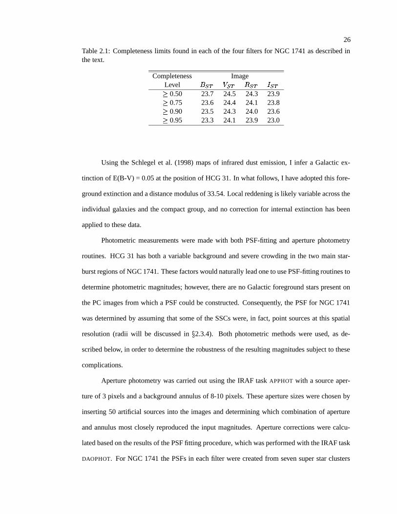
26
Table 2.1: Completeness limits found in each of the four filters for NGC 1741 as described inthe text.
Completeness ImageLevel
� � � � � � � � � � ��0.50 23.7 24.5 24.3 23.9�0.75 23.6 24.4 24.1 23.8�0.90 23.5 24.3 24.0 23.6�0.95 23.3 24.1 23.9 23.0
Using the Schlegel et al. (1998) maps of infrared dust emission, I infer a Galactic ex-
tinction of E(B-V) = 0.05 at the position of HCG 31. In what follows, I have adopted this fore-
ground extinction and a distance modulus of 33.54. Local reddening is likely variable across the
individual galaxies and the compact group, and no correction for internal extinction has been
applied to these data.
Photometric measurements were made with both PSF-fitting and aperture photometry
routines. HCG 31 has both a variable background and severe crowding in the two main star-
burst regions of NGC 1741. These factors would naturally lead one to use PSF-fitting routines to
determine photometric magnitudes; however, there are no Galactic foreground stars present on
the PC images from which a PSF could be constructed. Consequently, the PSF for NGC 1741
was determined by assuming that some of the SSCs were, in fact, point sources at this spatial
resolution (radii will be discussed in � 2.3.4). Both photometric methods were used, as de-
scribed below, in order to determine the robustness of the resulting magnitudes subject to these
complications.
Aperture photometry was carried out using the IRAF task APPHOT with a source aper-
ture of 3 pixels and a background annulus of 8-10 pixels. These aperture sizes were chosen by
inserting 50 artificial sources into the images and determining which combination of aperture
and annulus most closely reproduced the input magnitudes. Aperture corrections were calcu-
lated based on the results of the PSF fitting procedure, which was performed with the IRAF task
DAOPHOT. For NGC 1741 the PSFs in each filter were created from seven super star clusters
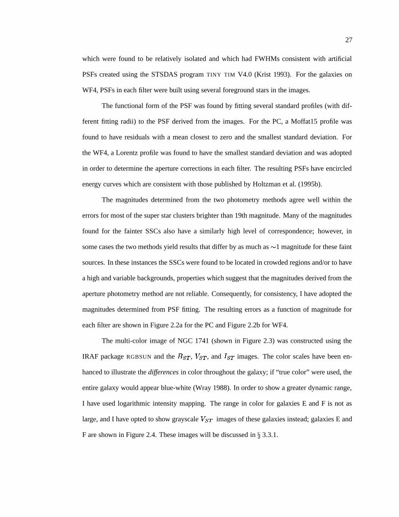
27
which were found to be relatively isolated and which had FWHMs consistent with artificial
PSFs created using the STSDAS program TINY TIM V4.0 (Krist 1993). For the galaxies on
WF4, PSFs in each filter were built using several foreground stars in the images.
The functional form of the PSF was found by fitting several standard profiles (with dif-
ferent fitting radii) to the PSF derived from the images. For the PC, a Moffat15 profile was
found to have residuals with a mean closest to zero and the smallest standard deviation. For
the WF4, a Lorentz profile was found to have the smallest standard deviation and was adopted
in order to determine the aperture corrections in each filter. The resulting PSFs have encircled
energy curves which are consistent with those published by Holtzman et al. (1995b).
The magnitudes determined from the two photometry methods agree well within the
errors for most of the super star clusters brighter than 19th magnitude. Many of the magnitudes
found for the fainter SSCs also have a similarly high level of correspondence; however, in
some cases the two methods yield results that differ by as much as � 1 magnitude for these faint
sources. In these instances the SSCs were found to be located in crowded regions and/or to have
a high and variable backgrounds, properties which suggest that the magnitudes derived from the
aperture photometry method are not reliable. Consequently, for consistency, I have adopted the
magnitudes determined from PSF fitting. The resulting errors as a function of magnitude for
each filter are shown in Figure 2.2a for the PC and Figure 2.2b for WF4.
The multi-color image of NGC 1741 (shown in Figure 2.3) was constructed using the
IRAF package RGBSUN and the� � �
, � � � , and � � � images. The color scales have been en-
hanced to illustrate the differences in color throughout the galaxy; if “true color” were used, the
entire galaxy would appear blue-white (Wray 1988). In order to show a greater dynamic range,
I have used logarithmic intensity mapping. The range in color for galaxies E and F is not as
large, and I have opted to show grayscale � � � images of these galaxies instead; galaxies E and
F are shown in Figure 2.4. These images will be discussed in � 3.3.1.
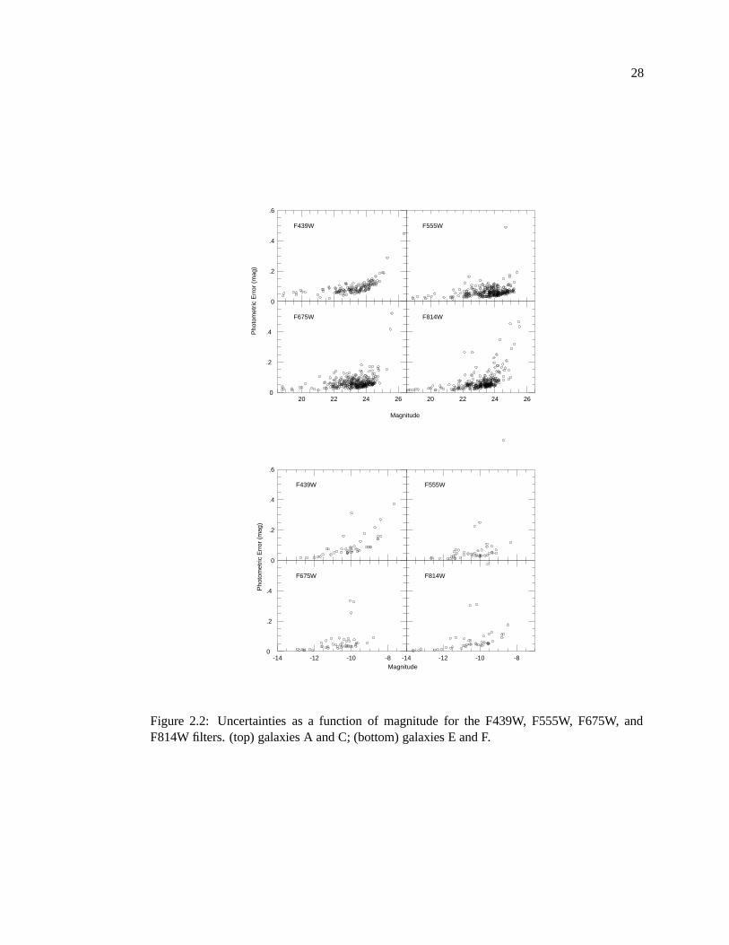
28
20 22 24 26
F675W
Magnitude
0
.2
.4Pho
tom
etric
Err
or (
mag
)
0
.2
.4
.6
F439W F555W
20 22 24 26
F814W
-14 -12 -10 -8
F675W
0
.2
.4
Magnitude
Pho
tom
etric
Err
or (
mag
)
0
.2
.4
.6
F439W F555W
-14 -12 -10 -8
F814W
Figure 2.2: Uncertainties as a function of magnitude for the F439W, F555W, F675W, andF814W filters. (top) galaxies A and C; (bottom) galaxies E and F.
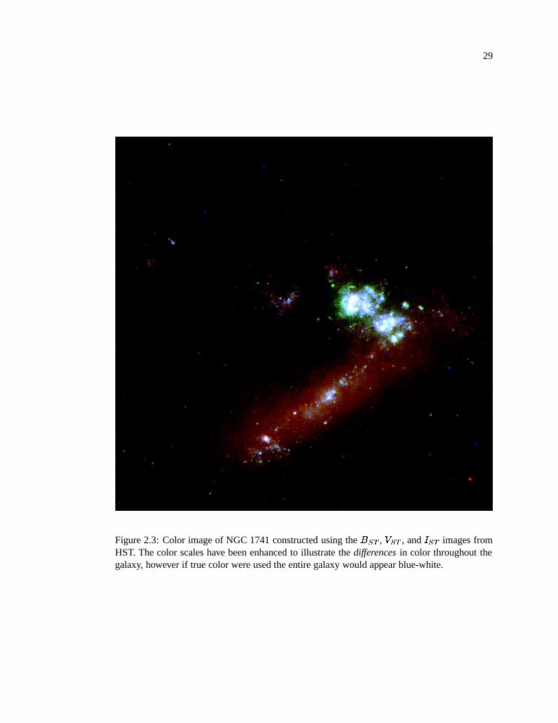
29
Figure 2.3: Color image of NGC 1741 constructed using the��� �
, � � � , and � � � images fromHST. The color scales have been enhanced to illustrate the differences in color throughout thegalaxy, however if true color were used the entire galaxy would appear blue-white.
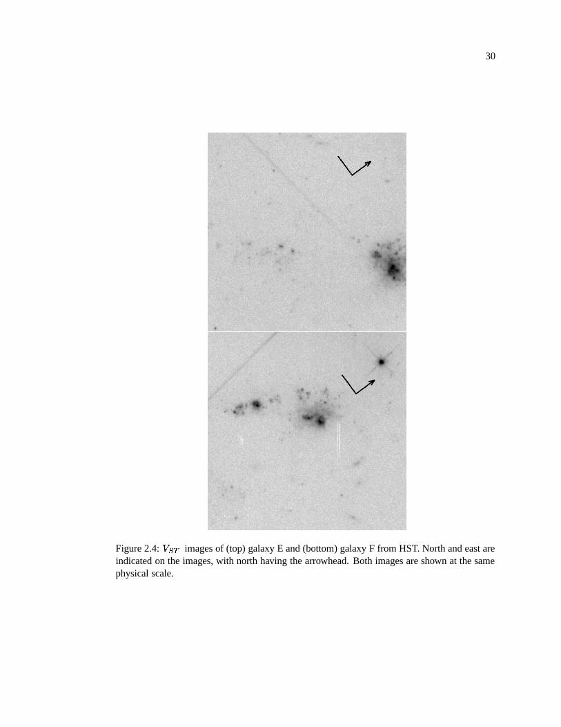
30
Figure 2.4: � � � images of (top) galaxy E and (bottom) galaxy F from HST. North and east areindicated on the images, with north having the arrowhead. Both images are shown at the samephysical scale.
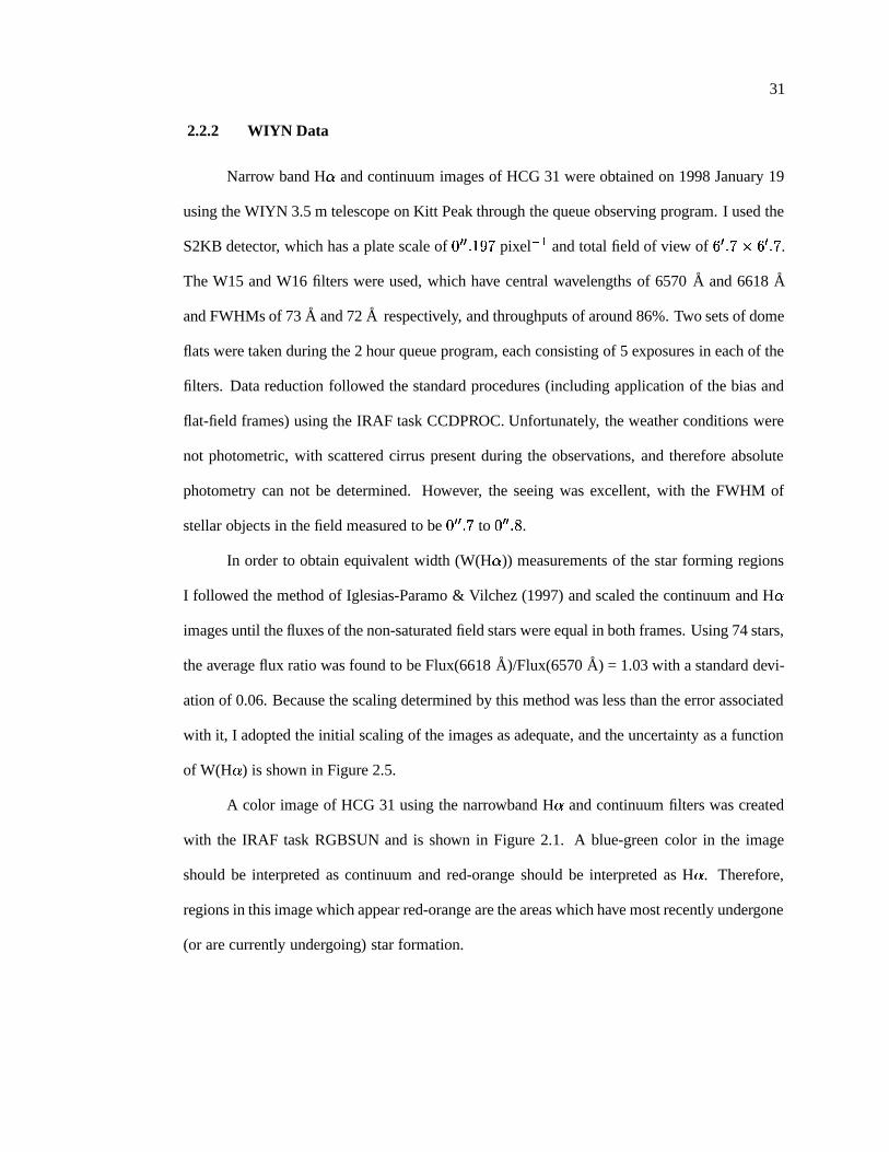
31
2.2.2 WIYN Data
Narrow band H � and continuum images of HCG 31 were obtained on 1998 January 19
using the WIYN 3.5 m telescope on Kitt Peak through the queue observing program. I used the
S2KB detector, which has a plate scale of � � � � � � � pixel � � and total field of view of � � � � � � � � � .The W15 and W16 filters were used, which have central wavelengths of 6570 A and 6618 A
and FWHMs of 73 A and 72 A respectively, and throughputs of around 86%. Two sets of dome
flats were taken during the 2 hour queue program, each consisting of 5 exposures in each of the
filters. Data reduction followed the standard procedures (including application of the bias and
flat-field frames) using the IRAF task CCDPROC. Unfortunately, the weather conditions were
not photometric, with scattered cirrus present during the observations, and therefore absolute
photometry can not be determined. However, the seeing was excellent, with the FWHM of
stellar objects in the field measured to be � � � � � to � � � � � .In order to obtain equivalent width (W(H � )) measurements of the star forming regions
I followed the method of Iglesias-Paramo & Vilchez (1997) and scaled the continuum and H �
images until the fluxes of the non-saturated field stars were equal in both frames. Using 74 stars,
the average flux ratio was found to be Flux(6618 A)/Flux(6570 A) = 1.03 with a standard devi-
ation of 0.06. Because the scaling determined by this method was less than the error associated
with it, I adopted the initial scaling of the images as adequate, and the uncertainty as a function
of W(H � ) is shown in Figure 2.5.
A color image of HCG 31 using the narrowband H � and continuum filters was created
with the IRAF task RGBSUN and is shown in Figure 2.1. A blue-green color in the image
should be interpreted as continuum and red-orange should be interpreted as H � . Therefore,
regions in this image which appear red-orange are the areas which have most recently undergone
(or are currently undergoing) star formation.
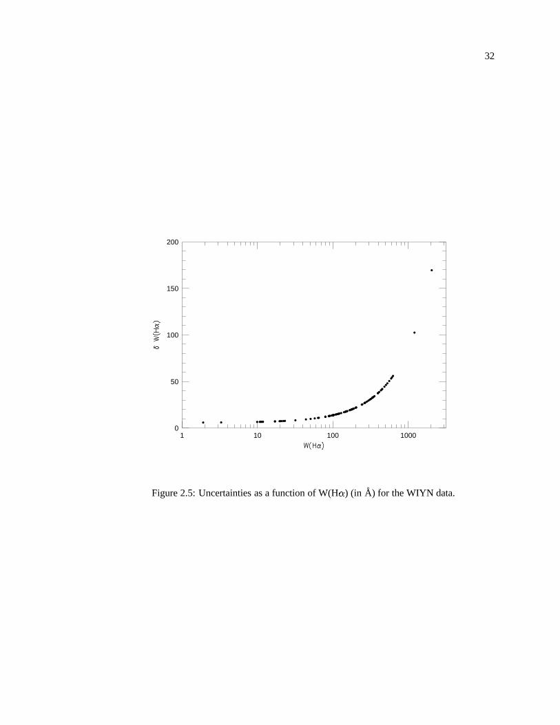
32
1 10 100 10000
50
100
150
200
Figure 2.5: Uncertainties as a function of W(H � ) (in A) for the WIYN data.

33
2.3 Results
2.3.1 Optical Morphology
H � emission traces recent star formation activity, and the W(H � ) can be used to estimate
the ages of recent episodes of star formation (Leitherer & Heckman 1995). As a stellar popula-
tion ages, the rate at which it produces H-ionizing photons decreases. For a case B ionization
bounded nebulae, the decrease in ionizing photons results in a decrease of the re-emitted Balmer
series photons relative to the continuum photons, and the W(H � ) will diminish over time.
The morphology of the H � emission in the galaxies of HCG 31 is highly irregular and
disturbed (Figure 2.1). The interaction site of galaxies A and C has the most prodigious H �
emission of the group, although there are several other locations with substantial values. As
well as the main starburst region in AC, there is also star formation on the eastern end of the
bar corresponding to galaxy A and some weaker H � emission coming from the ends of the tidal
tails extending to the north-east. The HST images resolve the main starburst region in AC into
numerous individual star clusters. Star clusters are also apparent at this resolution throughout
the entire body of AC. In addition, possible dust lanes and clumps are present in galaxy A,
which allow for the possibility of continued star formation. The star formation in galaxy B has
been resolved in several regions, most of which lie in the outer regions of the galaxy closest to
and furthest from galaxy AC — thus strongly indicative of the recent star formation in galaxy
B being due to tidal activity.
Galaxy E is connected to galaxy AC by a string of star-forming regions that may be
too small to be called galaxies themselves, but are not clearly associated with either galaxy
AC or galaxy E. Galaxy E itself appears to have two components — on the eastern side there
is a region of very recent star formation, and on the western side there is a region which has
no H � emission, and seems to be composed solely of an older generation of stars (possibly
lending support, in this case, for the stellar dynamical model of TDG formation). The HST
images resolve these two components into numerous SSCs and reveal that the younger region
34
is actually much smaller in spatial extent.
Galaxy F is the shy wall-flower of HCG 31, which has been too near a bright star to
the north-east to be studied until these high spatial resolution images became available. This
“galaxy” has two distinct components which are contained in the same peak of the H I emission
(Williams et al. 1991), but which do not appear to be physically connected by either continuum
or H � emission. In fact, the entire galaxy is very faint in the continuum image, but has W(H � )
measures that rival those of the starburst region in galaxy AC. As with galaxy E, the HST images
also resolve the two components into several SSCs. The lack of any evidence for an underlying
older stellar population may lend credence to the hydrodynamical theories of TDG formation
in this case (contrary to galaxy E).
Galaxy G has a roughly spherical shape in the continuum image, but is very asymmetric
in its H � emission with the star forming regions forming a U-shape along the north-west side.
There is some H � emission from the central region of this galaxy, but it is much less intense
than the regions along the north-west rim of the galaxy. It has been suggested previously by
Iglesias-Paramo & Vilchez (1997) that the strange star formation morphology is created by a
pressure/stripping mechanism, similar to the star formation seen in galaxies that are moving
through a high pressure medium. Here I propose an alternative way of looking at this mecha-
nism: gas may be preferentially inflowing to galaxy G from the direction of the main body of
the H I cloud in which HCG 31 is embedded, regardless of the direction of motion of galaxy G
relative to the ambient gas.
There are several small, low surface brightness features with only continuum light be-
tween galaxies E, F, and G. As above, these regions are not obviously associated with any of the
galaxies in the group, and due to their lack of H � emission, I interpret them as older populations
of stars that were tidally removed from one or more of the galaxies in the group.
35
2.3.2 Properties of the Super Star Clusters Compared to Models
2.3.2.1 Broad band magnitudes and colors
The colors of SSCs in combination with population synthesis models can yield informa-
tion about their ages, masses, and extinctions. The best population synthesis models available
for interpreting the colors of SSCs are those of Leitherer et al. (1999). Unfortunately, these
models do not include the contributions to the filter magnitudes from nebular line emission.
Since nebular lines can be very strong for starburst ages less than 10 Myr, and I suspect that
many SSCs in NGC 1741 may have such young ages (due to the presence of W-R features, see
VC and CLV), nebular line emission may significantly affect the colors. Therefore, we 1 have
developed new models based on work presented by Leitherer & Heckman (1995) that include
nebular line emission. This has an impact on the colors, particularly colors constructed from
the F555W filter. This filter is wider than Johnson V and includes the [OIII]� �
4959,5007 lines
that make substantial contributions to the F555W band flux at ages � � � Myr.
In Figure 2.6 the� � � �� � � and � � � � � � � color-color plot is shown. In Figures 2.7,
the observed � � � � � � � color vs � � � magnitude of the SSCs in NGC 1741 and galaxies E and F
are plotted along with the predicted colors and magnitude as a function of age given by the new
models containing nebular line emission. I have also plotted the model predictions for stellar
light only (i.e., without the nebular line emission). The reddening vector shown is for� � � �
adopted from the Calzetti et al. (1994) extinction law for starburst galaxies. Since these data
have not been corrected for internal reddening, one would correct for reddening by moving the
data points in the direction of the arrow.
While the locations of many of the SSCs in the color-color plot are consistent with the
models that include nebular line emission, the colors of some clusters are not consistent with
either set of models. Furthermore, the colors of all the brightest clusters are reproduced by
only those models which do not contain nebular line emission. Metallicity ( � ) can have a1 This work was carried out by C. Leitherer, and is presented in Johnson et al. (1999).
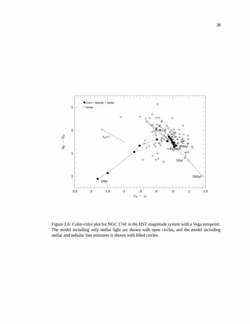
36
-2.5 -2 -1.5 -1 -.5 0 .5 1 1.5
2
1
0
-1
1Myr
10Myr100Myr
Lines + Nebular + Stellar
Stellar
1Gyr
10Gyr
Figure 2.6: Color-color plot for NGC 1741 in the HST magnitude system with a Vega zeropoint.The model including only stellar light are shown with open circles, and the model includingstellar and nebular line emission is shown with filled circles.
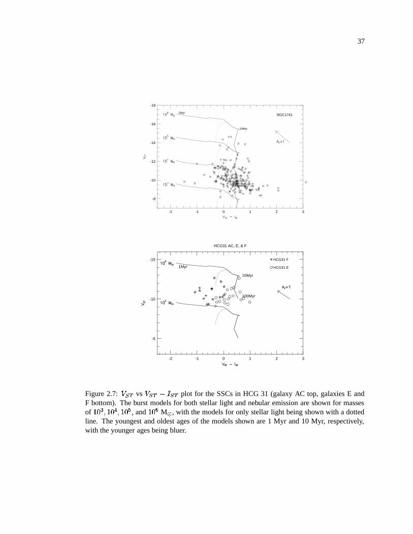
37
-2 -1 0 1 2 3
-8
-10
-12
-14
-16
-18
1Myr
10Myr
NGC1741
-2 -1 0 1 2 3
-5
-10
-15 HCG31 F
HCG31 E1Myr
10Myr
100Myr
HCG31 AC, E, & F
Figure 2.7:��� �
vs��� ����� � �
plot for the SSCs in HCG 31 (galaxy AC top, galaxies E andF bottom). The burst models for both stellar light and nebular emission are shown for massesof � � � � � � � and � � M � , with the models for only stellar light being shown with a dottedline. The youngest and oldest ages of the models shown are 1 Myr and 10 Myr, respectively,with the younger ages being bluer.
38
significant effect on the colors of starburst galaxies. Cervino & Mas-Hesse (1994) have shown
that, for ages between 3 and 10 Myr,� � and
���are sensitive to the colors of red supergiants,
which in turn are dependent on the metallicity of the galaxy; lower metallicity will tend to
make the colors bluer (see also Leitherer & Heckman 1995)). The models plotted here are for
0.25 Z (the value derived from the [O III]�
4363 line; see VC). It is also important to note
that stellar evolution models for red supergiants are notoriously uncertain (Mayya 1997), and
the predictions of evolutionary synthesis models with metal-poor red supergiants may not be
correct. A second explanation for the anomalous colors of some of the SSCs could be a diffuse
nebular background, which would be subtracted in � � � (due to the presence of [O III] and H�
)
but not in � � � – therefore tending to make the � � � � � � � color redder. This effect would be
important if the SSCs had blown away much of their surrounding material in our line of sight,
they were not optically thin to the background nebular emission, or we are primarily seeing
SSCs on the near side of the galaxy due to extinction.
It is evident from the color-color plots that most of the SSCs in NGC 1741 which have
been detected are younger than � � � Myr, regardless of which model is adopted. To estimate
the ages, extinctions, and masses of the clusters, I have developed a program that attempts to fit
magnitudes derived from population synthesis models (adjusted for reddening) to the observed
filter magnitudes. For each source, the age, reddening, and mass are determined from the best
fitting (in a least squares sense) model. Using this method, I find the median extinction of the
SSCs to be� � � � � � (E(B-V) � � � � ), which is in reasonable agreement with other studies, the
median age to be � � Myr, and the median mass � � � � � � M . However, one should bear in
mind that these are only average values and not representative of any specific SSC.
Although it is possible to put some limits on the ages and extinctions of SSCs using this
method, it is not possible to absolutely disentangle age and reddening for any given SSC using
only the broad-band colors for two reasons. First, the effects of age and reddening are nearly
degenerate. The reddening vector in Figure 2.7 is nearly parallel to the model that includes only
stellar continuum, and therefore the colors of older SSCs and more reddened SSCs would be
39
nearly identical to each other in this region. Second, if the SSCs are density bounded rather
than ionization bounded, it is not possible to determine a priori how much nebular continuum
and line emission should be included in the model for a given SSC.
In Figure 2.7, the � � � vs � � � � � � � color-magnitude diagram for the SSCs is plot-
ted along with the predicted evolutionary tracks for super star clusters with a range of masses
as derived from both sets of theoretical models (purely stellar light and stellar-plus-nebular
emission). Note that the models including nebular line emission have simply been scaled to
different masses without varying the ionization parameter. The youngest ages are bluest, with
� � � � � � � ��� � � � for models including nebular emission, and � � � � � � � ��� � � � for the
models including only stellar light, at an age of � Myr. The models turn over at 10 Myr as
the hottest stars from the initial burst die away, and are plotted until 100 Myr. From this plot
it is clear that most of the SSCs detected in NGC 1741 have masses between � � � � � � and
� � � M depending on the amount of extinction adopted (one should note that these results are
for a Salpeter IMF between 1 and 100� ; if the IMF extends below 1
� , these mass es-
timates will be correspondingly higher). Given the differential extinction in NGC 1741, with
quoted values ranging from � � � � � � � � � � ���� � � � (Iglesias-Paramo & Vilchez 1997), and the
obvious variation in environments throughout the galaxy as seen in Figure 2.3, it is probably
inappropriate to assume a single value for the entire galaxy; therefore, I have not applied any
correction for intrinsic extinction in the host galaxy.
In Figure 2.7, it is clear that both galaxies E and F have undergone substantial star for-
mation in the past 10 Myr. Moreover, the � � � - � � � colors of the SSCs in galaxy F are offset
blueward from those in galaxies A, C, and E. There is no indication of SSCs older than about
4 Myr in galaxy F, and most of the SSC colors are only consistent with the models including
nebular line emission. The requirement for nebular line emission not only implies that the SSCs
are very young, but also suggests there is little, if any, leakage of Lyman continuum photons
from them. The mean � � � - � � � color of SSCs in HCG31E is similar to that of HCG31A
and C, although there is less of a spread in color. The narrower color dispersion could be due
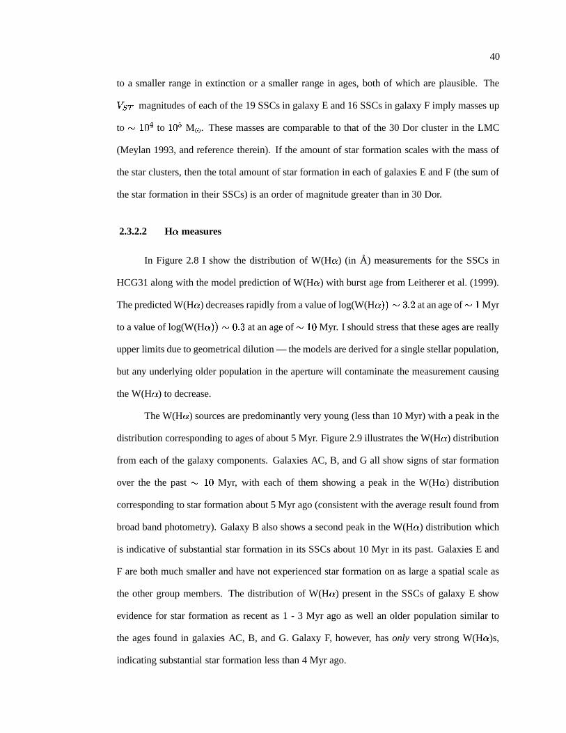
40
to a smaller range in extinction or a smaller range in ages, both of which are plausible. The
� � � magnitudes of each of the 19 SSCs in galaxy E and 16 SSCs in galaxy F imply masses up
to � � � � to � � � M . These masses are comparable to that of the 30 Dor cluster in the LMC
(Meylan 1993, and reference therein). If the amount of star formation scales with the mass of
the star clusters, then the total amount of star formation in each of galaxies E and F (the sum of
the star formation in their SSCs) is an order of magnitude greater than in 30 Dor.
2.3.2.2 H � measures
In Figure 2.8 I show the distribution of W(H � ) (in A) measurements for the SSCs in
HCG31 along with the model prediction of W(H � ) with burst age from Leitherer et al. (1999).
The predicted W(H � ) decreases rapidly from a value of log(W(H � � � � � � � at an age of � � Myr
to a value of log(W(H � � � � � � � at an age of � � � Myr. I should stress that these ages are really
upper limits due to geometrical dilution — the models are derived for a single stellar population,
but any underlying older population in the aperture will contaminate the measurement causing
the W(H � ) to decrease.
The W(H � ) sources are predominantly very young (less than 10 Myr) with a peak in the
distribution corresponding to ages of about 5 Myr. Figure 2.9 illustrates the W(H � ) distribution
from each of the galaxy components. Galaxies AC, B, and G all show signs of star formation
over the the past � � � Myr, with each of them showing a peak in the W(H � ) distribution
corresponding to star formation about 5 Myr ago (consistent with the average result found from
broad band photometry). Galaxy B also shows a second peak in the W(H � ) distribution which
is indicative of substantial star formation in its SSCs about 10 Myr in its past. Galaxies E and
F are both much smaller and have not experienced star formation on as large a spatial scale as
the other group members. The distribution of W(H � ) present in the SSCs of galaxy E show
evidence for star formation as recent as 1 - 3 Myr ago as well an older population similar to
the ages found in galaxies AC, B, and G. Galaxy F, however, has only very strong W(H � )s,
indicating substantial star formation less than 4 Myr ago.
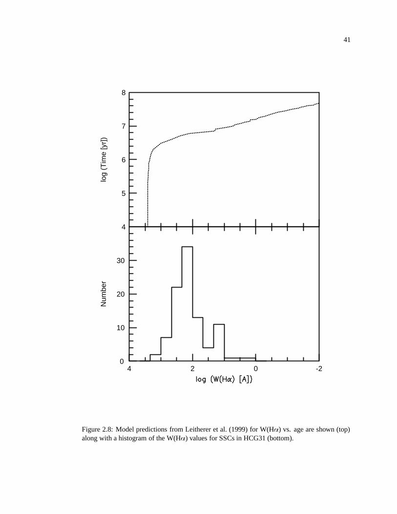
41
4
5
6
7
8
log
(Tim
e [y
r])
Num
ber
4 2 0 -20
10
20
30
Figure 2.8: Model predictions from Leitherer et al. (1999) for W(H � ) vs. age are shown (top)along with a histogram of the W(H � ) values for SSCs in HCG31 (bottom).
42
0
10
20AC
0
5B
0
5
Num
ber
E
0
5F
4 3 2 1 00
5G
Figure 2.9: A histogram of the W(H � ) values for SSCs in each of the member galaxies ofHCG31. Higher W(H � ) values correspond to younger ages.
43
Because the observing conditions were not photometric, I was not able to determine
absolute H � luminosities; I refer the reader to Iglesias-Paramo & Vilchez (1997) where they
measured H � luminosities for several starburst regions in HCG31.
2.3.3 Luminosity Functions of the Super Star Clusters
The � -band luminosity function (LF) for the SSCs in NGC 1741 is shown in Figure 2.10
with magnitudes presented in the Johnson system to facilitate comparisons with previous work
(the small number of SSCs in galaxies E and F undermine the statistical usefulness of perform-
ing this exercise on these galaxies). Detections beyond the completeness limit are shown by a
dotted line. The dashed line shows a power-law fit of the form ��� ��� � � � � over the range
from�
� � � � � � � mag to the completeness limit of�
� � � � � � mag, where I also expect
the brightest individual stars of NGC 1741 to start contributing to the LF (see below). No at-
tempt has been made to account for confusion, but it is possible that confused sources may
flatten the LF by a small amount. The best fit was determined by the method of least squares
with the data weighted by Poisson statistics. The best-fit power-law index was found to be by
� � � � � � � � � � � . There is no indication of a turnover in the luminosity function brightward of
our completeness limit.
In Figure 2.11 the Johnson � � � color distribution for the SSCs is shown. The mean
value was found to be � � � � � � � � with a dispersion of 0.49. As will be discussed in � 3.4,
these values can be used to place the SSCs in NGC 1741 in context with other starburst galaxy
cluster systems.
2.3.4 Cluster Radii
The radii of the sources were estimated in a manner similar to that of Whitmore et al.
(1993). First I created artificial Gaussian “sources” with effective radii in the range of 0.01-10
pixels. These artificial sources were then convolved with the PSFs of the three filters to mimic
how the sources would appear in the HST images. The magnitudes of these test objects were
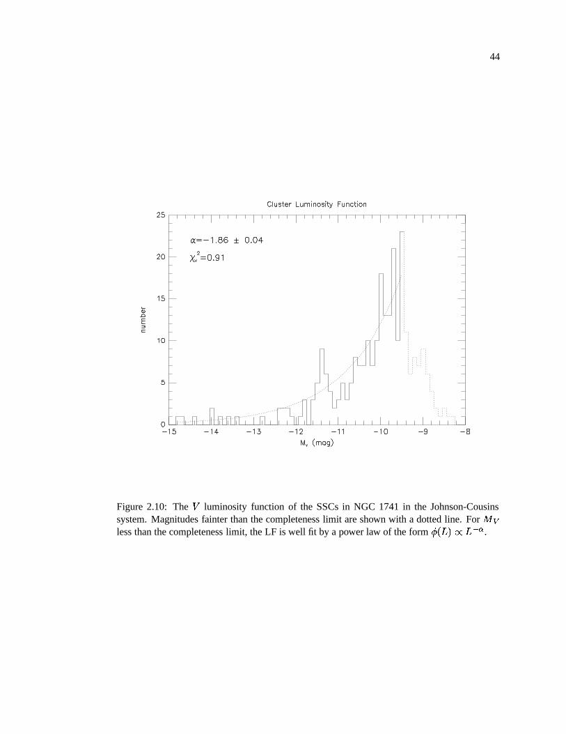
44
Figure 2.10: The � luminosity function of the SSCs in NGC 1741 in the Johnson-Cousinssystem. Magnitudes fainter than the completeness limit are shown with a dotted line. For
���less than the completeness limit, the LF is well fit by a power law of the form ��� ����� � � � .
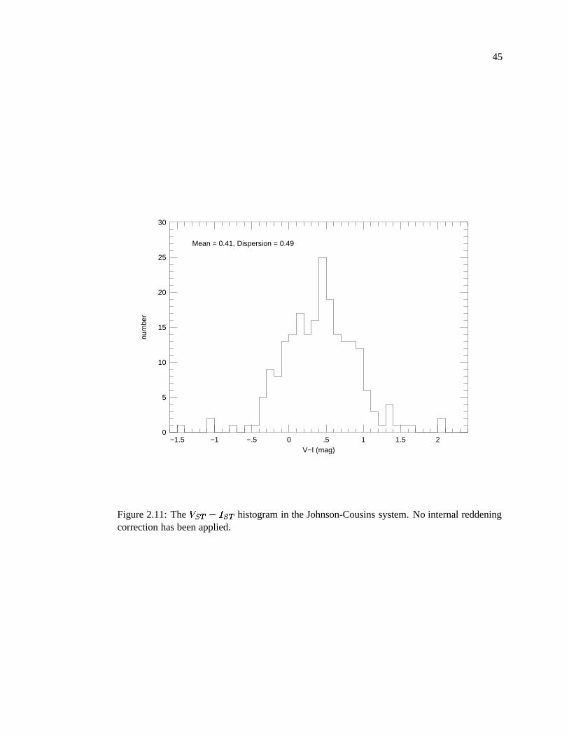
45
−1.5 −1 −.5 0 .5 1 1.5 20
5
10
15
20
25
30
Mean = 0.41, Dispersion = 0.49
V−I (mag)
num
ber
Figure 2.11: The � � � � � � � histogram in the Johnson-Cousins system. No internal reddeningcorrection has been applied.
46
then measured for several aperture values, and the differences in magnitude between apertures
of varying size were computed to determine which combination of apertures could best be used
to estimate the true size of the sources. In accord with Whitmore et al. (1993), I found that the
difference between the radii of r=0.5 and r=3 pixel apertures gave good results. However, at
radii values � � � pixels, this magnitude difference becomes nearly degenerate, and radii larger
than this value have extremely large uncertainties. The relation between the � � � � � magnitudes
and the effective radii for the F555W image is shown in Figure 2.12.
These test objects were then inserted into the actual F555W, F658N, and F814W images
at 50 random locations, and ��� � �� was measured to determine whether this method would be
reliable for the sources. The ��� � �� values found from this procedure had standard deviations
of � � � � , with the most inconsistent results coming from crowded regions or locations with
sharply varying backgrounds — both of which will tend to cause the sources to appear larger
than they actually are. However, overall this method proved to be quite reliable. The radii
measurements determined for the sources in the F555W filter are shown in Figure 2.13. Most
(90%) of the sources have radii values smaller than 3 pc, consistent with most of them being
unresolved. As Whitmore et al. (1993) and others have found, the effective radii of the brighter
SSCs appear to be larger near the central starburst region; there is also some evidence for this
trend in the present data. However, because of the substantial crowding and variable background
present almost ubiquitously in strong starbursts, I believe this to be an artifact of the method
and not likely to reflect the physical sizes.
2.3.5 The Burst Luminosity
The percentage of the total luminosity due to the SSCs can be determined by summing
the total flux of the clusters, and dividing by the total flux of the underlying galaxy. However,
there are two complicating factors. As the luminosity function illustrates, there is no indication
of a turnover at or above our completeness limit, and the number of fainter SSCs present but not
detected may continue to rise below our completeness limit. Due to the number of fainter SSCs
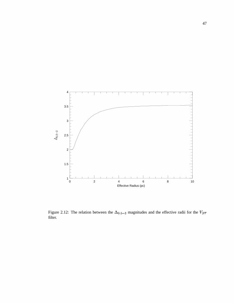
47
0 2 4 6 8 101
1.5
2
2.5
3
3.5
4
Effective Radius (pc)
Figure 2.12: The relation between the ��� � �� magnitudes and the effective radii for the � � �filter.
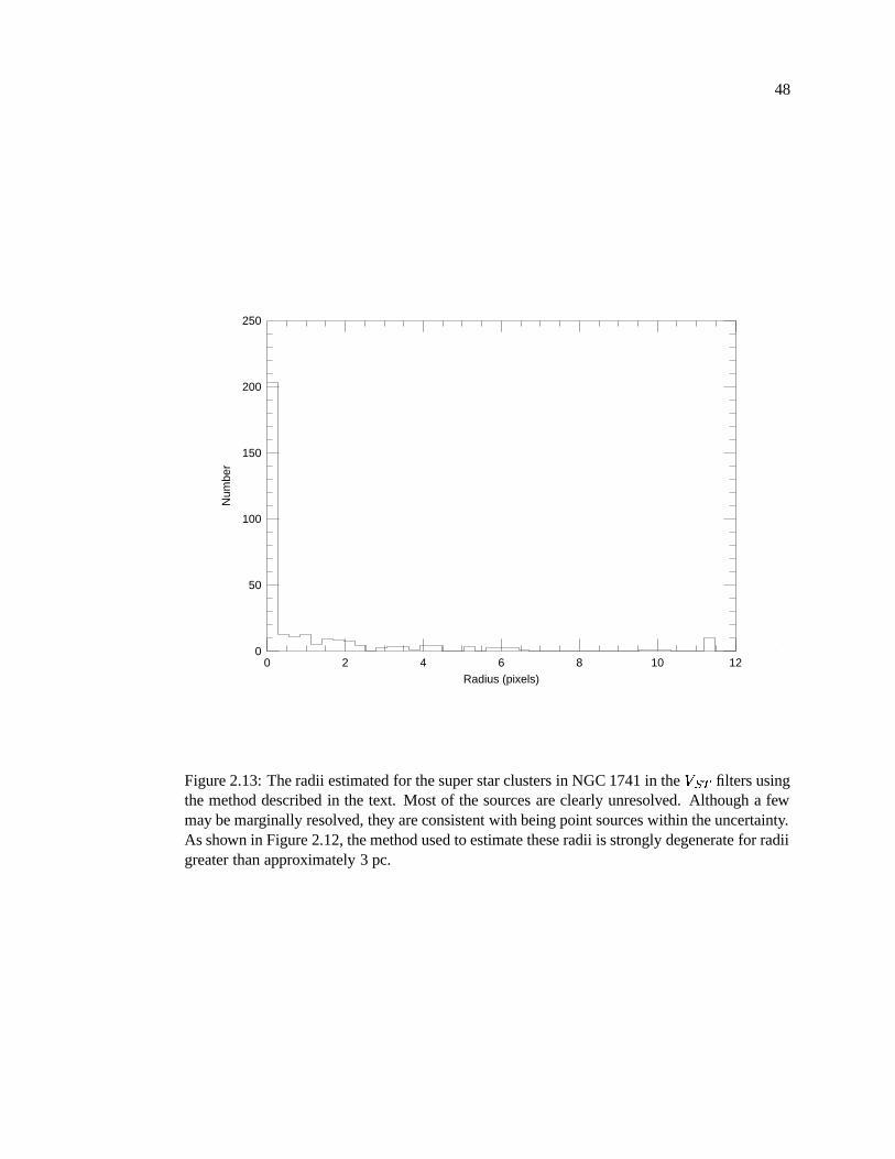
48
0 2 4 6 8 10 120
50
100
150
200
250
Radius (pixels)
Num
ber
Figure 2.13: The radii estimated for the super star clusters in NGC 1741 in the � � � filters usingthe method described in the text. Most of the sources are clearly unresolved. Although a fewmay be marginally resolved, they are consistent with being point sources within the uncertainty.As shown in Figure 2.12, the method used to estimate these radii is strongly degenerate for radiigreater than approximately 3 pc.
49
which may be excluded from this sample, the total burst luminosity is uncertain and should be
treated as a lower limit. The second complication is that defining the boundary of the galaxy is
not straightforward. Customarily the Holmberg radius (the level at which the surface brightness
is 26.5 mag arcsec ��� ) is used to determine the boundary. In his original survey to catalog
compact groups of galaxies, one of Hickson’s criteria was that the mean surface brightness be
� 26.0 (Hickson 1982), therefore for many galaxies within Hickson Compact Groups it is not
possible to use the Holmberg radius. In the case of NGC 1741, the surface brightness never
drops below this threshold anywhere on the PC chip. Another method commonly used is to
define the� � contour as the boundary of irregular galaxies. However, this method depends on
the signal to noise of the observation and therefore cannot be a consistent and reliable method
for the purpose of defining the boundaries of galaxies.
Hickson (1982) determined that the average surface brightness on red photographic
plates of HCG 31 is � � � � � � � � mag arcsec ��� . This value was used to differentiate between
galaxy flux and background flux. The flux inside this contour was calculated and the re-
sulting colors are consistent when converted to the same magnitude system with those pre-
viously published (Iglesias-Paramo & Vilchez 1997),� � � � � � � � � � � � � � � � � � � � � �
� � � � � � � � � � � � � � � � . However, these values are highly dependent on the isophotal contour
used to define the galaxy as shown in Figure 2.14. The percentage luminosity of the starburst
clusters is 5.1% in� � �
, typical of what has been found for other starburst systems. Meurer
et al. (1995) measured the fractional light contribution to the total light at 2200 A of 85 star
clusters in 9 starburst galaxies. On average, � 20% of the UV light comes from clusters. Since
super star clusters are bluer than the main body of the galaxy, this fraction is expected to de-
crease at longer wavelengths. Therefore the 5% contribution in��� �
by clusters in NGC 1741
is quite typical of that for starburst galaxies.

50
23 22.5 22 21.5 21 20.5 20 19.5 19-.2
0
.2
.4
.6
.8
23 22.5 22 21.5 21 20.5 20 19.5 19-.2
0
.2
.4
.6
.8
Figure 2.14: The isophotal dependence of the� � � � � � �
and� � � ��� � �
colors for the inte-grated light from NGC 1741. It is clear that the derived colors of the galaxy are dependent onthe boundary used.
51
2.4 Discussion
I now address several issues concerning the galaxies in HCG 31, including their dynami-
cal state, the properties and future of the SSCs, and the relevance to galaxies recently discovered
at redshift � � � . Although broad-band imaging alone does not allow us to address in detail
some of the interesting issues involving star formation in HCG 31, it is possible to gain sub-
stantial insight from the estimates provided by the results presented in this chapter.
2.4.1 The Star Formation History of HCG 31
It was previously noted by Iglesias-Paramo & Vilchez (1997) that all of the galaxies in
HCG 31 appear to have undergone their most recent episode of star formation almost simulta-
neously; they suggest the interaction of galaxies A and C was the triggering mechanism. The
results in this chapter would also seem to support contemporaneous star formation � � Myr
ago. However, it is unclear how instantaneous star formation could occur on such a short time
scale over such a large volume. Given the size of HCG 31 ( � � � kpc), it would take � � Gyr
for a super sonic shock speed of 50 km s ��� to propagate from one side of the group to the other
(at a typical sound speed of � � � km s ��� this propagation would take correspondingly longer;
for a discussion of star formation triggered by shocks see Vanhala & Cameron 1998, and refer-
ences therein). Furthermore, an interaction time scale of � � � � Myr can be derived based on
the length of the tidal tails and the rotation velocity (J. Hibbard, private communication).
Therefore, if this merger has been occurring for the past� � � Myr we are left with four
alternatives: (1) the group-wide recent peak in star formation is a coincidence; (2) the formation
of starbursts is a relatively recent event in the merger process, which implies there is a very
special time during the merger process; (3) there is some mechanism at work which does not
rely on shock propagation that has caused simultaneous and recent star formation throughout
HCG31; or (4) we are seeing only the most recent star formation, although star formation has
been occurring all along.
52
Although the first interpretation cannot be ruled out with certainty, something had to
trigger star formation in galaxies F and G that are quite distant from the main site of interaction
in galaxy AC. This is irrespective of whether the star formation has been occurring all along in
the HCG31 history or is a recent event.
Given the undoubtedly complicated history of HCG 31, the second interpretation is plau-
sible, but puzzling. For example, the complex velocity field of HCG 31 (Rubin et al. 1990)
suggests that neutral hydrogen flows are likely to intersect at speeds of several hundred km s ��� ,shock-heating the gas that then expands to fill the potential well of the group (Barnes 1997). If
the gas was too tenuous to cool rapidly, star formation could have been abated and/or delayed.
Under these conditions, it is possible that HCG 31 is undergoing a small scale cooling-flow sim-
ilar to those inferred for some large galaxy clusters (see Fabian 1994, and references therein).
This physical scenario might also be reflected in numerical simulations that have shown that
tidal material can remain bound to the merger system and return at later times (Barnes 1988;
Hernquist & Spergel 1992; Hernquist 1992, 1993). This process might lend support to the
third possibility that star formation has been simultaneously triggered by something other than
shocks.
The fourth possibility, that the older regions of star formation are simply not detected, is
undoubtedly true to some degree. The galaxies in the group almost certainly been undergoing
some level of star formation during the last crossing time of the group as the ambient gas
was torqued, shocked, and rapidly cooled thereby fueling star formation (Barnes & Hernquist
1991, 1996). From the population synthesis models it is possible to estimate the amount a
starburst will fade due to evolution. For ages between 10 and 100 Myr, a cluster will fade by
� 3 magnitudes; therefore, anything initially fainter than� � � � � � � � will be fainter than
our completeness limit at � � � Myr. Thus, many SSCs at that age are unlikely to be detected.
However, several SSCs brighter than� � � � � � � � are detected in NGC 1741 at this time and
there are relatively few SSCs with ages consistent with � ��� � Myr. Moreover, by the time a burst
has aged to 10 Myr, there will be virtually no H � emission, and the continuum emission will
53
have also faded by � � magnitude from its initial value (see the model predictions shown in
Figures 2.7 and 2.8). In fact, because the affects of age and reddening cannot be unambiguously
disentangled, several of the SSCs in galaxies AC and E are not inconsistent with having ages
��� � Myr (Figure 2.7). However, the bulk of them are young. The broad band colors of galaxy
F show no sign of star formation that could be older than � � Myr. Nevertheless, the possibility
that we are not dectecting the older star forming regions is viable within the completeness limit.
2.4.2 On the Youth of Galaxy F
As I have briefly discussed above, galaxy F appears to be the youngest galaxy in the
group. The broad-band colors of its SSCs are only consistent with a burst age of less than � �
Myr and it is the only galaxy in the HCG 31 that has only strong W(H � ) measurements indica-
tive of SSC ages no older than � � Myr. The fact that the broad-band colors might be affected
by some internal reddening and that the W(H � ) measurements may have been geometrically
diluted only serves to decrease the age of the starburst in galaxy F.
If galaxy F was seeded from tidal debris in the inter-group medium, then it is likely that
there is some older, underlying stellar population that was stripped from a parent galaxy in the
group. We can neither confirm nor deny this possibility with our current data. However, in color
images constructed from the WFPC2 filters, galaxy F is uniformly blue, even in lower surface
brightness regions with no SSCs. In contrast, galaxies AC and E, for which I have also made
three-color images, have blue starburst regions, but also show an underlying red (and therefore
older) stellar population. It would be useful to obtain deep far red or near IR spectra of galaxy F
in order to look for signatures of an older stellar population. Galaxy F may be a good example
of star formation triggered by collapse of molecular cloud material in the tidal tails, as proposed
by Elmegreen et al. (1993).
54
2.4.3 Globular Cluster Formation?
The characteristics observed for HCG 31, including the enhanced star formation, com-
plex morphology (including tidal tails), large-scale gradients in the H I map, and low velocity
dispersion of the group, suggest that HCG 31 is in the process of forming a single galaxy. In
fact, simulations (e.g., Barnes 1989) have shown that loose groups will evolve into compact
groups, which then typically merge into an elliptical galaxy. Such a scenario has direct impli-
cations for the interpretation of the SSCs in HCG 31. It has been observed that the number
of globular clusters per unit galaxy luminosity varies with the morphological type of the host
galaxy, with elliptical galaxies typically having a factor of 5 increase from the number seen in
late-type spirals. van den Bergh (1995) has argued based on the conservation of globular clus-
ters, that elliptical galaxies are not the merger remnants of spiral galaxies. However, if globular
clusters are formed during merger events, it may provide a simple explanation for the observed
abundance of globular clusters in ellipticals (Ashman & Zepf 1992).
In fact, there is now growing evidence that globular clusters (GCs) are indeed formed in
galactic interactions and mergers (Whitmore et al. 1993; Whitmore & Schweizer 1995; Meurer
et al. 1995; Schweizer et al. 1996). One question I wish to address is how the properties of
SSCs compare to those of GC systems of various ages. An evolutionary scenario relating SSCs
to GCs is developing in the literature based on luminosity functions, colors, radii, and masses
of observed systems in a variety of evolutionary states. I now add NGC 1741 to this picture as
a critical point for understanding the earliest stages of globular cluster formation.
The luminosity function of SSCs in NGC 1741 is well fit by a power law of the form
� � ��� � � � � � � � , and shows no sign of turning over brightward of the completeness limit at
��� � � � � � . This is consistent with the luminosity functions of other young clusters, with
exponents � � � � � � � � � (Vacca 1997; Schweizer et al. 1996; Whitmore & Schweizer 1995).
The luminosity function of galactic halo-type globular clusters with ages of � � � Gyr is roughly
Gaussian, with a peak magnitude of� � � � � , and therefore the lack of a turnover observed in
55
young systems such as NGC 1741 is significant. If globular clusters evolved from SSCs, evo-
lutionary models predict a peak at� � � � � � to � � � (depending on the amount of extinction
and the Hubble constant), which is at least 1.6 magnitudes brighter than our completeness limit.
However, there is no evidence for this turnover in our data.
One explanation for the lack of a turnover in our data is that most of the SSCs with
��� � � � � � may be disrupted as they age and evolve. Possible mechanisms for disruption
include two-body relaxation, tidal shocking, and dynamical friction. The time scale for an SSC
to disperse can be estimated by the dynamical time based on the virial theorem given by
� � � � � � � � � � �� � � � � � � � ����
where � � � is the effective radius in pc and� � is the mass of the SSC is units of � � � � (Vacca
1997). Given that the SSCs in NGC 1741 are unresolved, it is possible only to put an upper
limit on the radii of � � � pc. However, resolved SSCs typically have radii of � � � pc or less
(Schweizer et al. 1996; O’Connell et al. 1995; de Marchi et al. 1997) and this value is adopted.
As Figure 2.7 illustrates, the masses of the SSCs in NGC 1741 for a Salpeter-type IMF with an
upper and lower mass cutoff of � � � � and � � typically range between �� � � � � � � �
� � � � , consistent with the value of � � � � recently derived by Smith & Gallagher (2001) for
SSCs using velocity dispersions and the assumption of virial equilibrium. For our mass range,
the equation for� � � �
yields dynamical times of 20 Myr and 1.5 Myr respectively. Since SSCs
with ages older than the dynamical time can be considered bound, certainly some of SSCs I
have observed fit this criterion. However, most of the SSCs in NGC 1741 are younger than
20 Myr, and it is not possible to demonstrate whether they are bound using this method.
2.4.4 Comparison to Other Starburst Systems
It is useful to compare the properties of HCG 31 with those of other starbursts that have
been observed with HST. Schweizer et al. (1996) have observed a trend among merger systems
in which the mean � � � color of SSCs shifts from blue to red as the state of the merger
progresses. The mean value of � � � � � � � � for the SSCs found in NGC 1741 is bluer
56
than the youngest system currently available in their sample, NGC 4038/39, which has a mean
� � � � � � � � after a reddening correction of � � � � � mag. It is important to note that the values
for NGC 1741 have not had any reddening correction applied. Therefore, NGC 1741 provides
some of the youngest SSC systems currently available for study.
How does the star formation rate in NGC 1741 compare that in other starburst galaxies?
Gallagher et al. (1984) showed that the absolute blue luminosity is a useful tracer of this quan-
tity, although this method suffers from the obvious drawback that it must underestimate the star
formation rate to some extent due to the absorption of blue light by intervening dust. However,
the longer wavelength light (which is less likely to be extincted) also includes an increasingly
larger contribution from the older, evolved stellar population — therefore causing an overesti-
mation of the recent star formation rate. Using the Starburst99 models of Leitherer et al. (1999),
I can directly translate the B magnitude of NGC 1741 into a star formation rate. The B magni-
tude of the entire galaxy system (galaxies A + C) is� � � � � � � � . If the star formation has been
continuous over the last 10 Myr, this magnitude implies a star formation rate of 11.4 M yr � � .If I estimate the projected surface area of NGC 1741 to be � � � kpc � , I find a star-formation rate
per unit surface area of 0.3 M yr � � kpc � � for a Salpeter IMF between 1 and 100 M (again
note that if the IMF extends below 1 M , these star formation rates will be correspondingly
higher). However, the “burst” of star formation in NGC 1741 is not globally distributed in the
galaxy, rather it is predominantly taking place at the region of interaction between galaxies A
and C. The blue magnitude of this region alone is� � � � � � � � over an area � � � kpc � . The
corresponding star formation rate for this region is 7.2 M yr ��� or 0.7 M yr ��� kpc � � .Meurer et al. (1995, 1997) found that UV bright starburst galaxies have a very narrow
range in areal star-formation rate. In particular, they find an upper limit of 1.5 M yr ��� kpc ���(M � � � = 1 M ). The burst region in NGC 1741 follows the relationship of Meurer et al. The
areal star-formation rate of 0.7 M yr � � kpc � � is comparable to those found for the dwarf
starbursts NGC 3991 (0.8 M yr � � kpc � � ) or Tol 1924-416 (1.2 M yr � � kpc � � ). Furthermore,
this burst region of NGC 1741 has a star formation rate comparable to the typical values for the
57
total star formation rates of � � � � ���� � M yr � � for the high-redshift sample of Steidel et al.
(1996) and Lowenthal et al. (1997) (moduli the surface areas of the galaxies in those samples) ,
which justifies the status of NGC 1741 as a local template. For comparison, the star-formation
rates per unit surface area in normal disk galaxies (including the Milky Way) are about three
orders of magnitude lower (Meurer et al. 1997). NGC 1741 is a genuine starburst indeed!
Chapter 3
The Case of Henize 2-10
3.1 Background
Another galaxy in which we can study the starburst phenomenon and the formation of
super star clusters in Henize 2-10 (He 2-10). He 2-10 is a blue compact dwarf galaxy with
strong nebular features first detected in an H � survey of the southern sky (Henize 1967) and was
initially believed to be a planetary nebula. It has been the subject of numerous investigations
since Allen, Wright, & Goss (1976) first found the signatures of W-R stars in its integrated
optical spectrum, thus making He 2-10 the first known “Wolf-Rayet galaxy”. At a distance1
of 9 Mpc (� � � � � km s ��� Mpc � � ; Vacca & Conti 1992), He 2-10 is relatively nearby, and
has an optical diameter of � 2.8 kpc. He 2-10 has a high molecular gas content of � � � � �
M (Kobulnicky et al. 1995) and correspondingly high metallicity � ��� � (Kobulnicky et al. 1999).
The starburst activity in He 2-10 is concentrated in two regions, A and B (Vacca & Conti
1992), separated by �� �
( � 350 pc); the former is roughly at the optical center of the galaxy, the
latter almost directly east. W-R features were found in region A but not in region B (Vacca &
Conti 1992; Schaerer et al. 1999a). Using HST FOC images of He 2-10, Conti & Vacca (1994)
found that both starburst regions were composed of intense knots of (massive) stars. Recent
narrow band H � images of Mendez et al. (1999) reveal a kiloparsec-scale bipolar outflow
centered on region A, the most intense star forming region in the galaxy. This result indicates1 Distances have been suggested between 6 Mpc (Johansson 1987) and 14 Mpc (Allen et al. 1976) depending on
the choice of Virgocentric inflow model and���
.
59
that the recent starburst episode in He 2-10 has had a significant effect on its interstellar medium
and local environment.
The nature and history of the starburst in He 2-10 has been a subject of considerable
discussion in the literature. Johansson (1987) proposed that this starburst was the result of two
merging dwarf irregular galaxies. However, based on the smooth elliptical envelope well fit by
an � � � � law, Corbin et al. (1993) argued that the starburst activity is within a single dwarf ellipti-
cal galaxy undergoing stochastic star formation. Kobulnicky et al. (1995) detected a molecular
cloud extending to the south-east of the center of the galaxy, which is possibly falling into the
center of the galaxy and triggering the star formation.
Although the UV images of Conti & Vacca (1994) revealed the presence of SSCs in the
center of He 2-10, the estimation of their masses and ages required several assumptions, not the
least of which was the correction for internal extinction. Furthermore, ground-based images of
this object lack the resolution needed to study the properties of the individual knots. In � 3.2 I
present high spatial resolution optical images of He 2-10 obtained with HST. I determine some
of the parameters of the SSCs and consider the dust morphology of the starburst regions in � 3.3
using optical photometry. I will discuss the results, including the effect He 2-10 may have on
the intergalactic medium, in � 3.4.
3.2 Observations and Data Reduction
Optical images of He 2-10 were obtained on 1997 March 4 using the Wide Field and
Planetary Camera (WFPC2) aboard the Hubble Space Telescope (HST). Images were acquired
through two broad-band optical filters (F555W and F814W) and one narrow-band filter (F658N),
which corresponds to redshifted H � . In each filter, a set of exposures ( � ��� � � sec and � � � � sec)
were taken at each of two dithered positions. The 30 sec exposures were taken in case of sat-
uration on the 400 sec exposures; however, none of the galaxy images were saturated in the
region of interest, and the 30 sec exposures were not used. The dithering was done to regain
some of the spatial information lost by the under-sampling of the point spread function (PSF)

60
by WFPC2.
Both star-forming regions He 2-10 are completely contained on the PC, so we have
not analyzed the WF region of the images. The PC images were reduced following standard
pipeline procedures (including the application of bias, dark, and flat field frames) using the
Image Reduction and Analysis Facility (IRAF) and the Space Telescope Science Data System
(STSDAS). A correction for geometric distortion was applied to the images as prescribed by
Holtzman et al. (1995a), and the pairs of 400 sec images were combined using the STSDAS
task GCOMBINE, which also removes hot pixels and cosmic rays. The dithered images were
then combined using the “shift-and-add” technique: the images were block-replicated, dithered
offsets between these images were determined by the STSDAS task CROSSCOR, the images
were shifted by an integer number of pixels, and then the dithered pairs were combined. This
process resulted in final images of sizes 1600�
1600 pixels with 1 pixel � � � � � � � � � � . The
PHOTFLAM keyword in the image header was used to determine the photometric zeropoints,
with resulting magnitudes in the STMAG system. These magnitudes were then shifted to a
Vega zero point in order to facilitate comparisons, and we refer to them as � � � H � � � and
� � � (Holtzman et al. 1995a).
Using the Schlegel et al. (1998) maps of infrared dust emission, we infer a Galactic
extinction of E(B-V) = 0.11 at the position of He 2-10 (which has a Galactic latitude of � �� � � �
). In what follows, we have adopted this foreground extinction and a distance modulus of
� m � � � � � . As we only have two broad-band magnitudes, no correction for internal extinction
has been applied to these data. Local reddening is likely to be highly variable across He 2-10,
as is evidenced in Figure 3.1 and will be discussed in � 3.3.1.
Several hundred (mostly point-) sources were identified in each of the filters using the
IRAF task DAOFIND. A detection criterion of� � � above the local background level was used
to identify sources; below this threshold the number of spurious detections was uncomfortably
large (more than � 15% would have been rejected upon visual examination). The detections
in each filter were then visually inspected to check the identification, and a few sources were
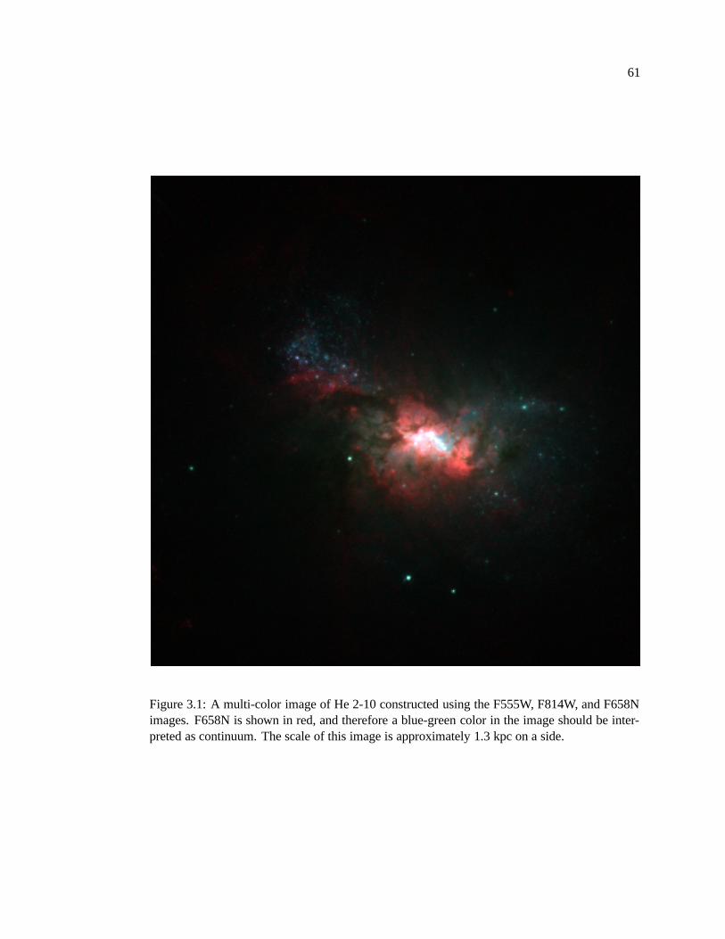
61
Figure 3.1: A multi-color image of He 2-10 constructed using the F555W, F814W, and F658Nimages. F658N is shown in red, and therefore a blue-green color in the image should be inter-preted as continuum. The scale of this image is approximately 1.3 kpc on a side.
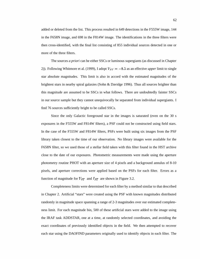
62
added or deleted from the list. This process resulted in 649 detections in the F555W image, 144
in the F658N image, and 698 in the F814W image. The identifications in the three filters were
then cross-identified, with the final list consisting of 855 individual sources detected in one or
more of the three filters.
The sources a priori can be either SSCs or luminous supergiants (as discussed in Chapter
2)). Following Whitmore et al. (1999), I adopt � � � � ��� � � as an effective upper limit to single
star absolute magnitudes. This limit is also in accord with the estimated magnitudes of the
brightest stars in nearby spiral galaxies (Sohn & Davidge 1996). Thus all sources brighter than
this magnitude are assumed to be SSCs in what follows. There are undoubtedly fainter SSCs
in our source sample but they cannot unequivocally be separated from individual supergiants. I
find 76 sources sufficiently bright to be called SSCs.
Since the only Galactic foreground star in the images is saturated (even on the 30 s
exposures in the F555W and F814W filters), a PSF could not be constructed using field stars.
In the case of the F555W and F814W filters, PSFs were built using six images from the PSF
library taken closest to the time of our observation. No library images were available for the
F658N filter, so we used those of a stellar field taken with this filter found in the HST archive
close to the date of our exposures. Photometric measurements were made using the aperture
photometry routine PHOT with an aperture size of 4 pixels and a background annulus of 8-10
pixels, and aperture corrections were applied based on the PSFs for each filter. Errors as a
function of magnitude for � � � and � � � are shown in Figure 3.2.
Completeness limits were determined for each filter by a method similar to that described
in Chapter 2. Artificial “stars” were created using the PSF with known magnitudes distributed
randomly in magnitude space spanning a range of 2-3 magnitudes over our estimated complete-
ness limit. For each magnitude bin, 500 of these artificial stars were added to the image using
the IRAF task ADDSTAR, one at a time, at randomly selected coordinates, and avoiding the
exact coordinates of previously identified objects in the field. We then attempted to recover
each star using the DAOFIND parameters originally used to identify objects in each filter. The
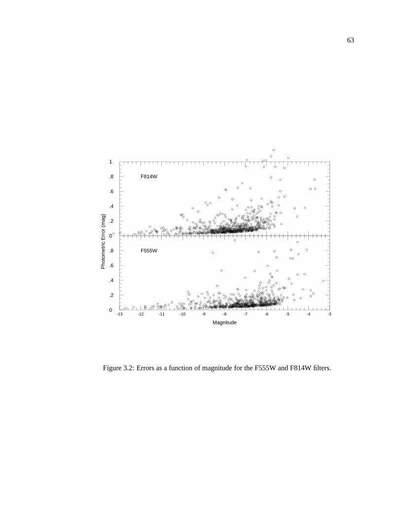
63
-13 -12 -11 -10 -9 -8 -7 -6 -5 -4 -3
Magnitude
F555W
0
.2
.4
.6
.8
F814W
0
.2
.4
.6
.8
1
Pho
tom
etric
Err
or (
mag
)
Figure 3.2: Errors as a function of magnitude for the F555W and F814W filters.
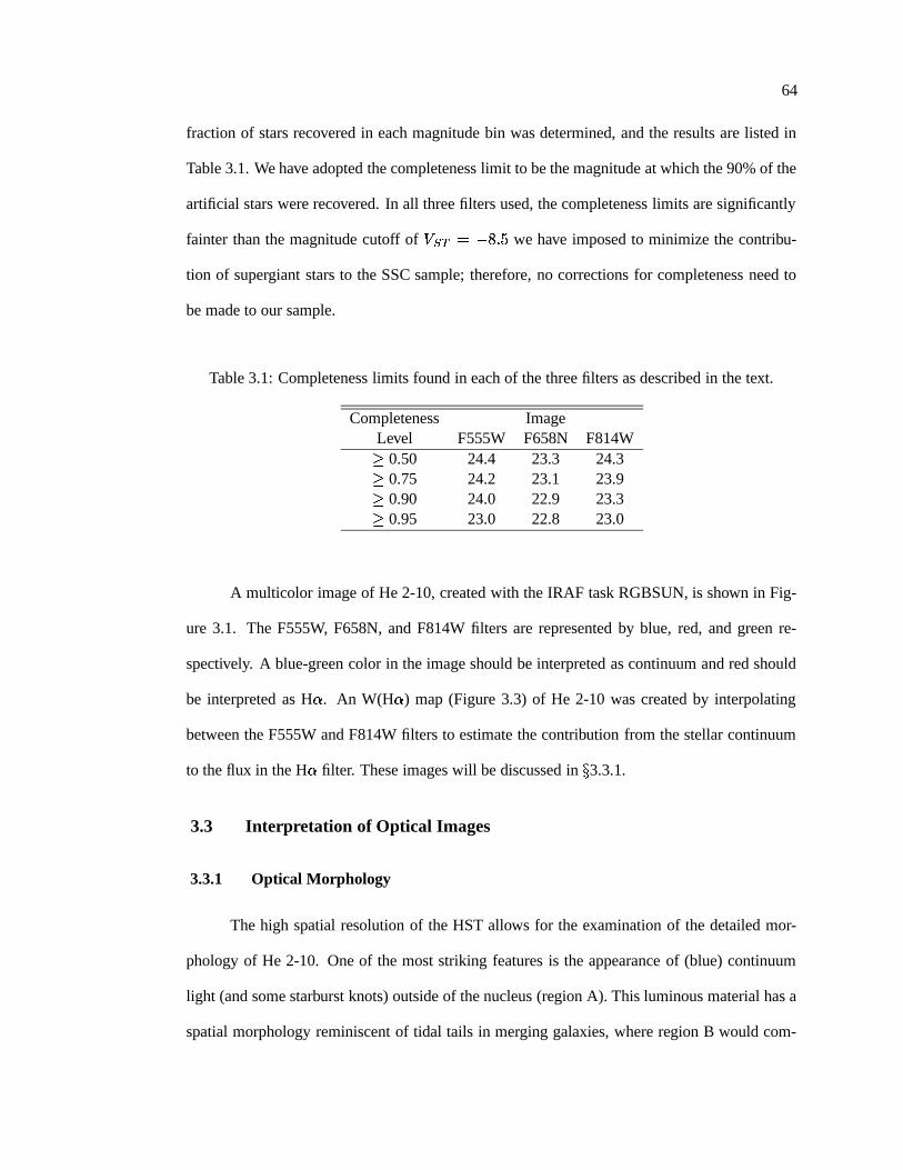
64
fraction of stars recovered in each magnitude bin was determined, and the results are listed in
Table 3.1. We have adopted the completeness limit to be the magnitude at which the 90% of the
artificial stars were recovered. In all three filters used, the completeness limits are significantly
fainter than the magnitude cutoff of � � � � ��� � � we have imposed to minimize the contribu-
tion of supergiant stars to the SSC sample; therefore, no corrections for completeness need to
be made to our sample.
Table 3.1: Completeness limits found in each of the three filters as described in the text.
Completeness ImageLevel F555W F658N F814W�
0.50 24.4 23.3 24.3�0.75 24.2 23.1 23.9�0.90 24.0 22.9 23.3�0.95 23.0 22.8 23.0
A multicolor image of He 2-10, created with the IRAF task RGBSUN, is shown in Fig-
ure 3.1. The F555W, F658N, and F814W filters are represented by blue, red, and green re-
spectively. A blue-green color in the image should be interpreted as continuum and red should
be interpreted as H � . An W(H � ) map (Figure 3.3) of He 2-10 was created by interpolating
between the F555W and F814W filters to estimate the contribution from the stellar continuum
to the flux in the H � filter. These images will be discussed in � 3.3.1.
3.3 Interpretation of Optical Images
3.3.1 Optical Morphology
The high spatial resolution of the HST allows for the examination of the detailed mor-
phology of He 2-10. One of the most striking features is the appearance of (blue) continuum
light (and some starburst knots) outside of the nucleus (region A). This luminous material has a
spatial morphology reminiscent of tidal tails in merging galaxies, where region B would com-

65
Figure 3.3: A map of the W(H � ) in He 2-10, where the brighter colors correspond to largerequivalent widths. North and east are indicated on the image, with north having the arrowhead.This image is shown with the same scale and orientation as Figure 3.1 — the length of thecompass arms is approximately 100 pc.
66
prise one “tail” (which Johansson 1987, proposed was the interacting dwarf galaxy companion),
and a smaller “tail” stretching to the north-west. The multicolor image, Figure 3.1, also reveals
several features which appear to be dust lanes, including an extensive lane between regions A
and B and another WNW of region A. The former is located near the position of the densest
region of the molecular cloud detected at radio wavelengths by Kobulnicky et al. (1995). The in-
terpretation of these features as dust lanes is further strengthened by moderate spatial resolution
ground-based infrared images, which reveal large� ��� colors in these regions (Vacca 2000,
private communication). The HST data suggests that the apparent galaxy morphology (e.g., the
separation between the two galaxy components and the “tidal tail” morphology) is primarily a
result of a dust lane blocking the light from part of the galaxy behind it, a possibility which
calls into question the interpretation of region B as a separate dwarf galaxy. While there is no
compelling evidence for an interacting second stellar system within He 2-10, the trigger for the
starburst activity in this object could be the elongated molecular cloud found by Kobulnicky
et al. (1995). This cloud is� � � � in length, is aligned south-east, and appears to be falling into
the center of the galaxy. Admittedly, this material is within the volume of the dwarf elliptical,
not a usual location for tidal material, but its geometry is suggestive.
The dust lanes might be hiding other star forming regions. Indirect evidence for large
and highly variable amounts of local dust obscuration with� �
of up to about 17 magnitudes
has been found by Kawara et al. (1989) (see also Phillips et al. 1984; Beck et al. 1997). In
addition, Kobulnicky & Johnson (1999) have detected five thermal radio sources that are highly
obscured and not present in optical images but which have luminosities similar to those of the
known SSCs, which will be discussed in Chapter 4. Nevertheless, since both starburst regions
are visible in the optical and UV (Conti & Vacca 1994) the extinction cannot be uniformly high
in those directions, although dust might hide activity on the far side of the galaxy center.
The H � emission is distributed diffusely throughout the galaxy. The morphology in
the W(H � ) (Figure 3.3) image is strikingly different from that seen in the F555W image in
Figure 3.4. Filaments extending from the south and to the east of region A can be seen in the
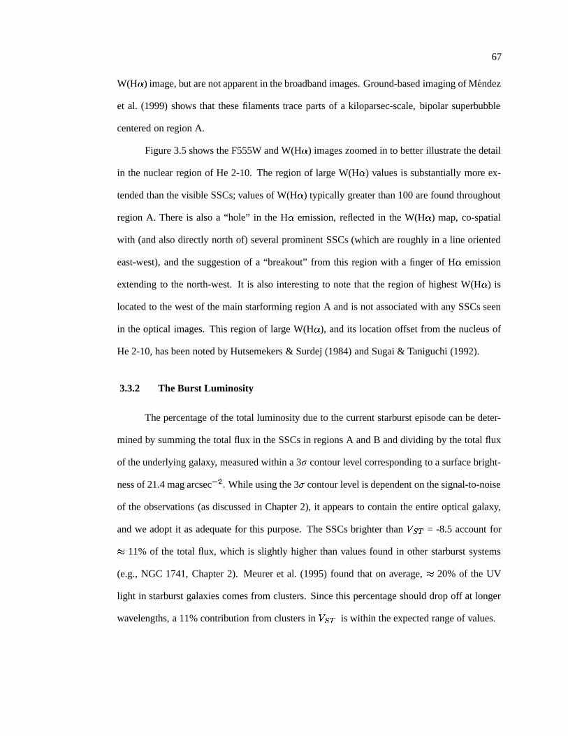
67
W(H � ) image, but are not apparent in the broadband images. Ground-based imaging of Mendez
et al. (1999) shows that these filaments trace parts of a kiloparsec-scale, bipolar superbubble
centered on region A.
Figure 3.5 shows the F555W and W(H � ) images zoomed in to better illustrate the detail
in the nuclear region of He 2-10. The region of large W(H � ) values is substantially more ex-
tended than the visible SSCs; values of W(H � ) typically greater than 100 are found throughout
region A. There is also a “hole” in the H � emission, reflected in the W(H � ) map, co-spatial
with (and also directly north of) several prominent SSCs (which are roughly in a line oriented
east-west), and the suggestion of a “breakout” from this region with a finger of H � emission
extending to the north-west. It is also interesting to note that the region of highest W(H � ) is
located to the west of the main starforming region A and is not associated with any SSCs seen
in the optical images. This region of large W(H � ), and its location offset from the nucleus of
He 2-10, has been noted by Hutsemekers & Surdej (1984) and Sugai & Taniguchi (1992).
3.3.2 The Burst Luminosity
The percentage of the total luminosity due to the current starburst episode can be deter-
mined by summing the total flux in the SSCs in regions A and B and dividing by the total flux
of the underlying galaxy, measured within a 3 � contour level corresponding to a surface bright-
ness of 21.4 mag arcsec � � . While using the 3 � contour level is dependent on the signal-to-noise
of the observations (as discussed in Chapter 2), it appears to contain the entire optical galaxy,
and we adopt it as adequate for this purpose. The SSCs brighter than � � � = -8.5 account for
� 11% of the total flux, which is slightly higher than values found in other starburst systems
(e.g., NGC 1741, Chapter 2). Meurer et al. (1995) found that on average, � 20% of the UV
light in starburst galaxies comes from clusters. Since this percentage should drop off at longer
wavelengths, a 11% contribution from clusters in � � � is within the expected range of values.
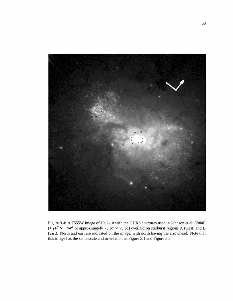
68
Figure 3.4: A F555W image of He 2-10 with the GHRS apertures used in Johnson et al. (2000)( � � � � � � � � � � � � � or approximately 75 pc
�75 pc) overlaid on starburst regions A (west) and B
(east). North and east are indicated on the image, with north having the arrowhead. Note thatthis image has the same scale and orientation as Figure 3.1 and Figure 3.3.
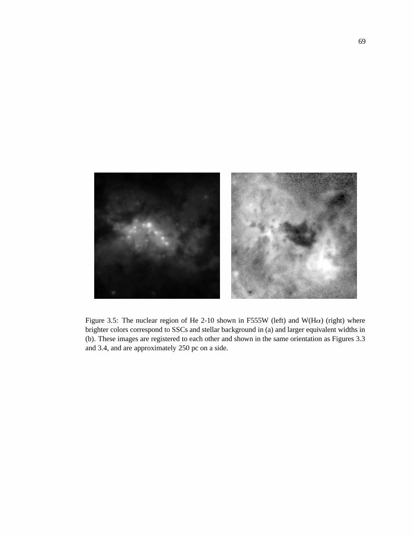
69
Figure 3.5: The nuclear region of He 2-10 shown in F555W (left) and W(H � ) (right) wherebrighter colors correspond to SSCs and stellar background in (a) and larger equivalent widths in(b). These images are registered to each other and shown in the same orientation as Figures 3.3and 3.4, and are approximately 250 pc on a side.
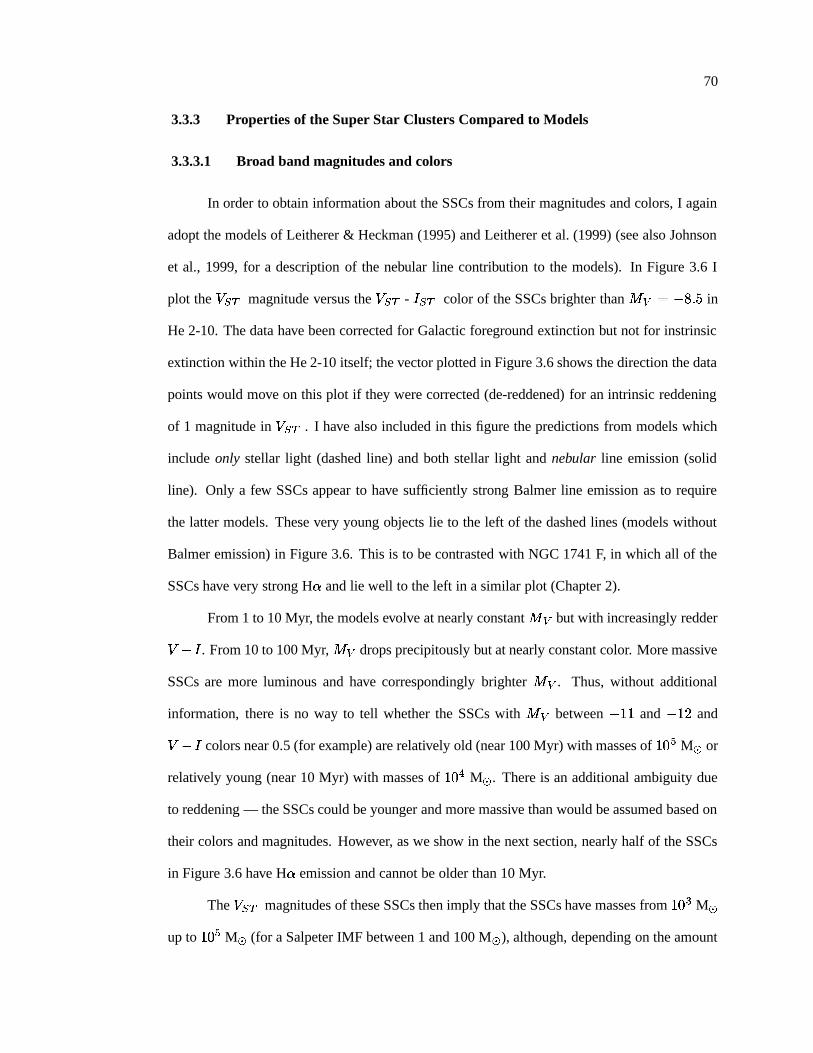
70
3.3.3 Properties of the Super Star Clusters Compared to Models
3.3.3.1 Broad band magnitudes and colors
In order to obtain information about the SSCs from their magnitudes and colors, I again
adopt the models of Leitherer & Heckman (1995) and Leitherer et al. (1999) (see also Johnson
et al., 1999, for a description of the nebular line contribution to the models). In Figure 3.6 I
plot the � � � magnitude versus the � � � - � � � color of the SSCs brighter than� � � ��� � � in
He 2-10. The data have been corrected for Galactic foreground extinction but not for instrinsic
extinction within the He 2-10 itself; the vector plotted in Figure 3.6 shows the direction the data
points would move on this plot if they were corrected (de-reddened) for an intrinsic reddening
of 1 magnitude in � � � . I have also included in this figure the predictions from models which
include only stellar light (dashed line) and both stellar light and nebular line emission (solid
line). Only a few SSCs appear to have sufficiently strong Balmer line emission as to require
the latter models. These very young objects lie to the left of the dashed lines (models without
Balmer emission) in Figure 3.6. This is to be contrasted with NGC 1741 F, in which all of the
SSCs have very strong H � and lie well to the left in a similar plot (Chapter 2).
From 1 to 10 Myr, the models evolve at nearly constant� �
but with increasingly redder
� � � . From 10 to 100 Myr,���
drops precipitously but at nearly constant color. More massive
SSCs are more luminous and have correspondingly brighter� �
. Thus, without additional
information, there is no way to tell whether the SSCs with� �
between � � � and � � � and
� � � colors near 0.5 (for example) are relatively old (near 100 Myr) with masses of � � � M or
relatively young (near 10 Myr) with masses of � � � M . There is an additional ambiguity due
to reddening — the SSCs could be younger and more massive than would be assumed based on
their colors and magnitudes. However, as we show in the next section, nearly half of the SSCs
in Figure 3.6 have H � emission and cannot be older than 10 Myr.
The � � � magnitudes of these SSCs then imply that the SSCs have masses from � � � M up to � � � M (for a Salpeter IMF between 1 and 100 M ), although, depending on the amount
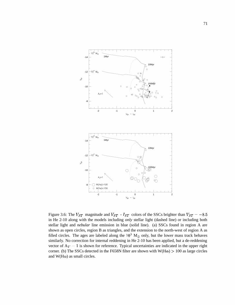
71
-2 -1 0 1 2
-8
-10
-12
-14 1Myr
10Myr
100Myr
-2 -1 0 1 2
-8
-10
-12
-14 1Myr
10Myr
100Myr
Figure 3.6: The� � �
magnitude and� � �
-� � �
colors of the SSCs brighter than� � � � ����� �
in He 2-10 along with the models including only stellar light (dashed line) or including bothstellar light and nebular line emission in blue (solid line). (a) SSCs found in region A areshown as open circles, region B as triangles, and the extension to the north-west of region A asfilled circles. The ages are labeled along the � M � only, but the lower mass track behavessimilarly. No correction for internal reddening in He 2-10 has been applied, but a de-reddeningvector of A � � � is shown for reference. Typical uncertainties are indicated in the upper rightcorner. (b) The SSCs detected in the F658N filter are shown with W(H � ) � 100 as large circlesand W(H � ) as small circles.
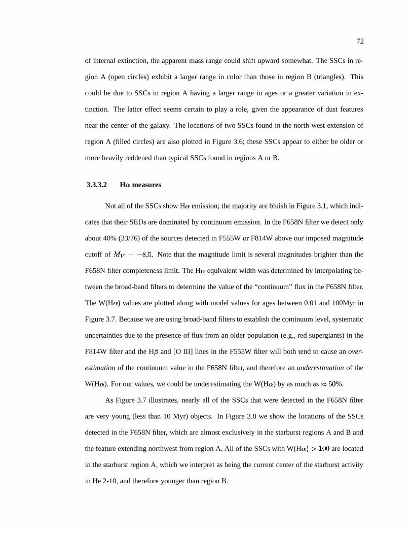
72
of internal extinction, the apparent mass range could shift upward somewhat. The SSCs in re-
gion A (open circles) exhibit a larger range in color than those in region B (triangles). This
could be due to SSCs in region A having a larger range in ages or a greater variation in ex-
tinction. The latter effect seems certain to play a role, given the appearance of dust features
near the center of the galaxy. The locations of two SSCs found in the north-west extension of
region A (filled circles) are also plotted in Figure 3.6; these SSCs appear to either be older or
more heavily reddened than typical SSCs found in regions A or B.
3.3.3.2 H � measures
Not all of the SSCs show H � emission; the majority are bluish in Figure 3.1, which indi-
cates that their SEDs are dominated by continuum emission. In the F658N filter we detect only
about 40% (33/76) of the sources detected in F555W or F814W above our imposed magnitude
cutoff of��� � ��� � � . Note that the magnitude limit is several magnitudes brighter than the
F658N filter completeness limit. The H � equivalent width was determined by interpolating be-
tween the broad-band filters to determine the value of the “continuum” flux in the F658N filter.
The W(H � ) values are plotted along with model values for ages between 0.01 and 100Myr in
Figure 3.7. Because we are using broad-band filters to establish the continuum level, systematic
uncertainties due to the presence of flux from an older population (e.g., red supergiants) in the
F814W filter and the H�
and [O III] lines in the F555W filter will both tend to cause an over-
estimation of the continuum value in the F658N filter, and therefore an underestimation of the
W(H � ). For our values, we could be underestimating the W(H � ) by as much as � � � %.
As Figure 3.7 illustrates, nearly all of the SSCs that were detected in the F658N filter
are very young (less than 10 Myr) objects. In Figure 3.8 we show the locations of the SSCs
detected in the F658N filter, which are almost exclusively in the starburst regions A and B and
the feature extending northwest from region A. All of the SSCs with W(H � � ��� � � are located
in the starburst region A, which we interpret as being the current center of the starburst activity
in He 2-10, and therefore younger than region B.
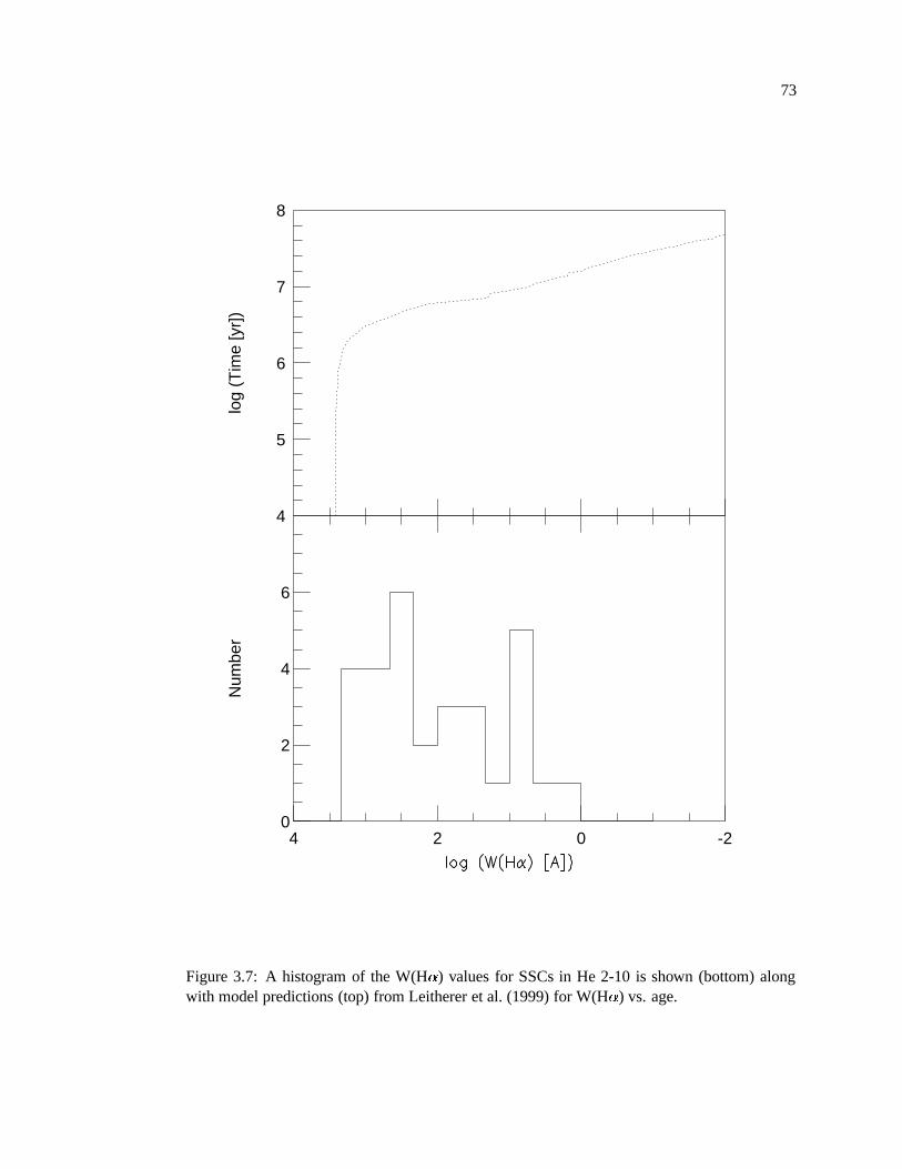
73
4
5
6
7
8
log
(Tim
e [y
r])
4 2 0 -2
Num
ber
0
2
4
6
Figure 3.7: A histogram of the W(H � ) values for SSCs in He 2-10 is shown (bottom) alongwith model predictions (top) from Leitherer et al. (1999) for W(H � ) vs. age.
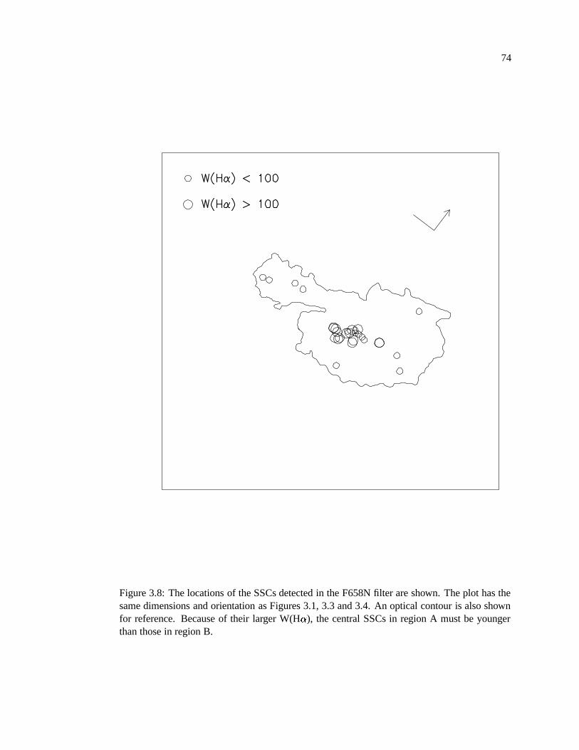
74
Figure 3.8: The locations of the SSCs detected in the F658N filter are shown. The plot has thesame dimensions and orientation as Figures 3.1, 3.3 and 3.4. An optical contour is also shownfor reference. Because of their larger W(H � ), the central SSCs in region A must be youngerthan those in region B.
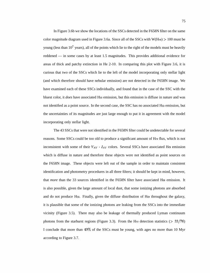
75
In Figure 3.6b we show the locations of the SSCs detected in the F658N filter on the same
color magnitude diagram used in Figure 3.6a. Since all of the SSCs with W(H � ) � 100 must be
young (less than 10 � years), all of the points which lie to the right of the models must be heavily
reddened — in some cases by at least 1.5 magnitudes. This provides additional evidence for
areas of thick and patchy extinction in He 2-10. In comparing this plot with Figure 3.6, it is
curious that two of the SSCs which lie to the left of the model incorporating only stellar light
(and which therefore should have nebular emission) are not detected in the F658N image. We
have examined each of these SSCs individually, and found that in the case of the SSC with the
bluest color, it does have associated H � emission, but this emission is diffuse in nature and was
not identified as a point source. In the second case, the SSC has no associated H � emission, but
the uncertainties of its magnitudes are just large enough to put it in agreement with the model
incorporating only stellar light.
The 43 SSCs that were not identified in the F658N filter could be undetectable for several
reasons. Some SSCs could be too old to produce a significant amount of H � flux, which is not
inconsistent with some of their � � � - � � � colors. Several SSCs have associated H � emission
which is diffuse in nature and therefore these objects were not identified as point sources on
the F658N image. These objects were left out of the sample in order to maintain consistent
identification and photometry procedures in all three filters; it should be kept in mind, however,
that more than the 33 sources identified in the F658N filter have associated H � emission. It
is also possible, given the large amount of local dust, that some ionizing photons are absorbed
and do not produce H � . Finally, given the diffuse distribution of H � throughout the galaxy,
it is plausible that some of the ionizing photons are leaking from the SSCs into the immediate
vicinity (Figure 3.5). There may also be leakage of thermally produced Lyman continuum
photons from the starburst regions (Figure 3.3). From the H � detection statistics ( �� � � � )
I conclude that more than� � �
of the SSCs must be young, with ages no more than 10 Myr
according to Figure 3.7.
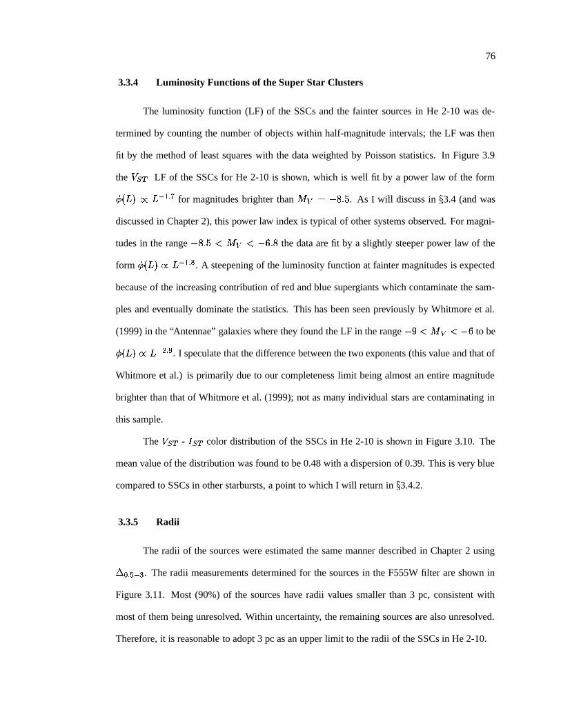
76
3.3.4 Luminosity Functions of the Super Star Clusters
The luminosity function (LF) of the SSCs and the fainter sources in He 2-10 was de-
termined by counting the number of objects within half-magnitude intervals; the LF was then
fit by the method of least squares with the data weighted by Poisson statistics. In Figure 3.9
the � � � LF of the SSCs for He 2-10 is shown, which is well fit by a power law of the form
��� ��� � ��� � � for magnitudes brighter than� � � ��� � � . As I will discuss in � 3.4 (and was
discussed in Chapter 2), this power law index is typical of other systems observed. For magni-
tudes in the range � � � � � ��� � � � � � the data are fit by a slightly steeper power law of the
form ��� ��������� � � . A steepening of the luminosity function at fainter magnitudes is expected
because of the increasing contribution of red and blue supergiants which contaminate the sam-
ples and eventually dominate the statistics. This has been seen previously by Whitmore et al.
(1999) in the “Antennae” galaxies where they found the LF in the range � � � ��� � � � to be
��� ����������� � . I speculate that the difference between the two exponents (this value and that of
Whitmore et al.) is primarily due to our completeness limit being almost an entire magnitude
brighter than that of Whitmore et al. (1999); not as many individual stars are contaminating in
this sample.
The � � � - � � � color distribution of the SSCs in He 2-10 is shown in Figure 3.10. The
mean value of the distribution was found to be 0.48 with a dispersion of 0.39. This is very blue
compared to SSCs in other starbursts, a point to which I will return in � 3.4.2.
3.3.5 Radii
The radii of the sources were estimated the same manner described in Chapter 2 using
� � � � � . The radii measurements determined for the sources in the F555W filter are shown in
Figure 3.11. Most (90%) of the sources have radii values smaller than 3 pc, consistent with
most of them being unresolved. Within uncertainty, the remaining sources are also unresolved.
Therefore, it is reasonable to adopt 3 pc as an upper limit to the radii of the SSCs in He 2-10.
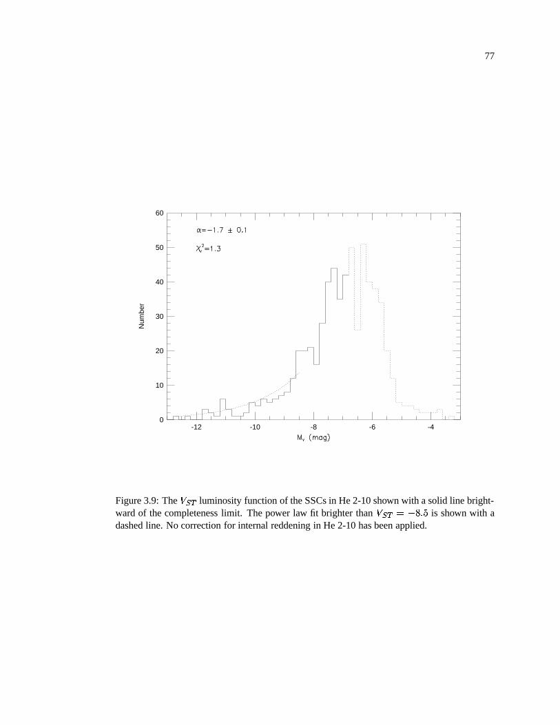
77
-12 -10 -8 -6 -40
10
20
30
40
50
60
Num
ber
Figure 3.9: The � � � luminosity function of the SSCs in He 2-10 shown with a solid line bright-ward of the completeness limit. The power law fit brighter than � � � � � � � � is shown with adashed line. No correction for internal reddening in He 2-10 has been applied.
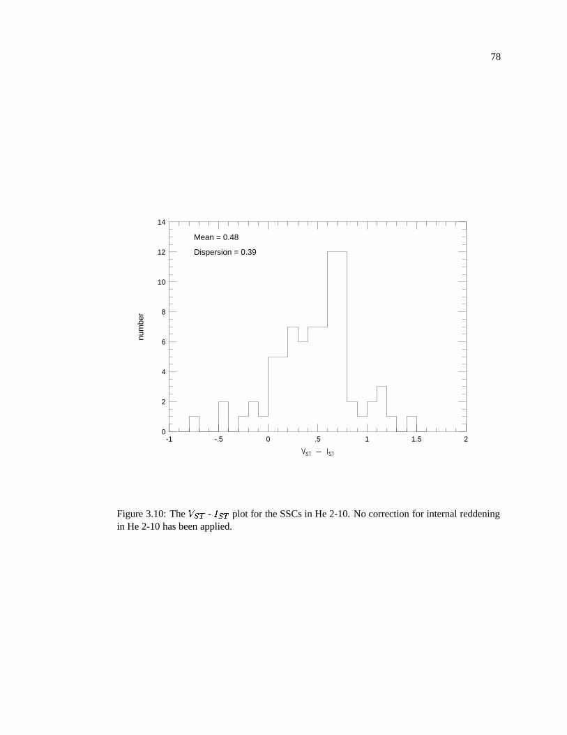
78
-1 -.5 0 .5 1 1.5 20
2
4
6
8
10
12
14
num
ber
Mean = 0.48
Dispersion = 0.39
Figure 3.10: The � � � - � � � plot for the SSCs in He 2-10. No correction for internal reddeningin He 2-10 has been applied.
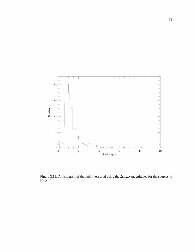
79
0 2 4 6 8 100
20
40
60
80
Radius (pc)
Num
ber
Figure 3.11: A histogram of the radii measured using the � � � � � magnitudes for the sources inHe 2-10.
80
3.4 Discussion
3.4.1 On the Universality of SSC Luminosity Functions
As discussed in Chapter 1, a universal mechanism for cluster formation has been pro-
posed by Elmegreen & Efremov (1997) who argue that the initial mass spectrum for star clus-
ters is naturally a power law with a slope of � ��� . This slope is the result of the hierarchical
distribution of structure in turbulent gas, and the primary differences between various types of
clusters (i.e., open clusters and globular clusters) are due to pressure differences in the cluster
birth environments.
The observed slope of the luminosity function for SSCs is dependent on the initial mass
spectrum of clusters, the ages of the SSCs, and the stellar initial mass function (IMF). In the
case of W-R galaxies, such as He 2-10, the age of the burst can be constrained a priori to �
3 to 6 Myr using evolutionary synthesis models 2 . Therefore, if we take the stellar IMF to be
universal, as recent work has suggested (see Massey et al. 1995; Massey & Hunter 1998), and
the luminosity functions of the SSCs W-R galaxies are compared, any similarities or differences
provide direct information about the initial mass spectrum of clusters. In Chapter 2 another W-R
galaxy was studied, NGC 1741, and found a power law slope of � � � � � � � � , in close agreement
with the value for He 2-10 of � � � � � � � � . Observations of other starburst galaxies yield similar
exponents for the LF of SSCs ( ��� � � � � � � � ; Vacca 1997; Schweizer et al. 1996; Whitmore
& Schweizer 1995; Meurer et al. 1995, see Table 1.1). Obviously more examples need to
be obtained, but this technique may be providing us with evidence of a constant initial mass
spectrum of SSCs.2 It should be noted that even in the case that star formation is not relatively instantaneous (as in a burst), if
clusters are formed with the same power law distribution at all times, the time integrated distribution will evolvewith the same power law distribution as that of an instantaneous burst.
81
3.4.2 Comparison to Other Starburst Systems
The mean � � � color of SSCs in interacting galaxies is predicted to shift from blue
to red with time (see Schweizer et al. 1996). Although He 2-10 is not an interacting system
in the classical sense, it does show evidence of interaction with a � � �
M molecular cloud (a
disturbed morphology and possible tidal tails), and it is appropriate to compare its star formation
history with other merger systems. The mean color of � � � � � � � � is among the bluest values
found for SSCs in interacting systems studied to date. This can be interpreted to mean that the
SSCs in He 2-10 are among the youngest identified. As discussed in Chapter 2, NGC 1741
is another example of extremely young system of SSCs with a mean color of � � � � � � � � ,before including any correction for internal reddening. In the sample studied by Schweizer
et al. (1996), the galaxy system with the bluest color distribution is NGC 4038/39 with a mean
� � � � � � � � after a reddening correction of -0.26 magnitudes. It is important to reiterate
here that our magnitudes of the SSCs in He 2-10 have not been corrected for internal reddening.
Furthermore, it is important to note that many of the knots seen in the optical WFPC2 images
are very bright in the FOC 2200 A image obtained by Conti & Vacca (1994). The strong UV
flux from these knots is an additional indicator of their young ages. Hence, He 2-10 provides an
example of some of the most recently formed SSCs ever observed, a point which I will expand
upon in Chapter 4.
How does the star formation rate in He 2-10 compare to other starburst systems? As in
chapter 2, the blue luminosity can be used to estimate the star formation rate. Adopting a B
magnitude of -19.1 from Conti (1991), the Starburst99 models of Leitherer et al. (1999) imply
a total star formation rate of 3.8 M yr � � if the star formation has been occurring over the
last 10 Myr (for a Salpeter IMF between 1 and 100 M ). Adopting a projected surface area of
He 2-10 to be ��� kpc � , the star formation rate per unit surface area is 1.3 M yr � � kpc � � . This
star formation rate is among the highest observed for UV-bright starburst galaxies (Meurer et al.
1995), and nearly twice as high as the star formation rate observed for the starburst in NGC 1741
82
in chapter 1. Given that star formation efficiencies necessary to form bound clusters are on the
order of � � � � (e.g., Verschueren 1990), an average star formation rate of 3.8 M yr ��� would
consume the molecular cloud mass of � � � �
M that appears to be interacting with and fueling
the starburst (Kobulnicky et al. 1995) in � � � � � � years. Therefore the molecular cloud is not
likely to fuel star formation at such a high rate over a very long time scale.
3.4.3 Implications of Large-Scale Outflow
The mechanical luminosity input from supernova-driven winds, and the resulting mass
outflows, can have a significant affect on the evolution of dwarf galaxies and the metal enrich-
ment and ionization of the IGM. In Johnson et al. (2000) we concluded that there is a large-scale
outflow of the interstellar medium in He 2-10 with a bulk motion of minimally 360 km s � � and
a mass of at least � � � M (based on the spectral analysis done by C. Leitherer and not presented
here). This outflow velocity is somewhat larger than the value of 250 km s � � that Mendez et al.
(1999) derive from ground-based spectroscopy of the bipolar superbubble centered on region A.
This discrepancy is likely due to geometrical effects, as we have spectra of different parts of the
galaxy, and therefore different inclination angles of the outflow. While outflows have been ob-
served in a number of galaxies (e.g., Pettini et al. 2000; Gonzalez Delgado et al. 1998; Kunth
et al. 1998; Marlowe et al. 1995; Heckman et al. 1995; Meurer et al. 1992), they are typically
� � � � km s ��� . The outflow we measure in He 2-10 has the one of the highest velocities ever
observed in cold gas via metal absorption lines (Ly � and Ly�
absorption components indicate
even higher velocities in a few galaxies, however Ly � is a complex line, affected by scattering,
and the picture is not clear, Gonzalez Delgado et al. 1998; Kunth et al. 1998).
In order to determine whether this outflow has a velocity high enough to result in mass
loss from He 2-10, an estimate of the escape velocity (�� ) needs to be obtained. The most
simplistic approach is to assume the escape is from a point source mass, implying
����� � � �
��� � � ������ � � � (3.1)
83
where�
is the dynamical mass and � is the current radius of the outflowing shell. Here I assume
the radius of the outflow is approximately the projected radius of the outflow of � � kpc found
by Mendez et al. (1999). Baas et al. (1994) estimated the dynamical mass of He 2-10 to be
� � � � ��� � � � �
M , and Kobulnicky et al. (1995) found the mass of He 2-10 to be � � � � � � � �
M (uncertain by a factor of � � sin� � � , where
�is the inclination angle of the bulk rotation). This
issue is somewhat complicated by the complex rotation curve, but here if I adopt the dynamical
mass of � � � � ��� � � � �
M , the escape velocity for He 2-10 is ��� � � � � � km s � � .I can also estimate the the
�� using the more sophisticated relation derived for dwarf
galaxies by Ferrara & Tolstoy (2000);
�� ��� � � ��� �
� � � � � ��� � ��� � (3.2)
where� ���
� is the dynamical mass in units of 10 � M and� � � � � � �
km s � � Mpc � � . Again
I adopt the dynamical mass of � � � � � ��� � � � � �
M and� � � � � � � � � � , implying the escape
velocity for He 2-10 is � � � � � � � km s � � . This value is in agreement with the the low end of
the range of escape velocities presented by Mendez et al. of 110 to 425 km s � � . Adopting the
range�� � � � � � � � km s ��� to
�� � � � � � � � km s � � , it is clear that the measured outflow
velocity of � 360 km s ��� is more than adequate to escape the gravitational potential well of
He 2-10.
Once the outflow has escaped He 2-10, it will be able to enrich the local IGM. Ferrara &
Tolstoy (2000) find the oxygen yield (the mass fraction of the stellar mass to be converted into
oxygen and expelled) to be 0.0871 for a Salpeter IMF, with lower and upper mass cutoffs of
1 M and 120 M , although this value may be an order of magnitude lower for low metallicity
stars in the � ��
universe (Woosley & Weaver 1995). (It is also important to bear in mind that
since stellar mass loss is primarily radiatively driven through metal lines, a low metallicity may
also inhibit the outflow to begin with.) From the UV spectrum, Johnson et al. (2000) estimated
the total stellar mass locked up in the current starburst episode in regions A and B to be � �
to� � � � � M (based on the spectral analysis done by C. Leitherer and not presented here);
84
this value is a lower limit as it does not include the contributions from the galaxy outside these
regions. We can roughly estimate this additional mass from the � � � magnitudes of SSCs not
included in the GHRS apertures as � � � � M . This total mass implies an expelled oxygen mass
of � � � � � � � � � � M . The models of Mac Low & Ferrara (1999) for metal ejection efficiency
for starburst-driven mass loss from dwarf galaxies indicate that virtually all of the metals ejected
by massive stars in He 2-10 will be lost from the galaxy. This mass in metals would be enough
to raise primordial metal abundances in 1 Mpc � to approximately 10 � � to 10 � � solar.
If the outflow continues to expand at � 360 km s ��� , it would take � 2 Gyr to travel
1 Mpc. However, one should note that the outflow is likely to be stopped before a radius of
1 Mpc due to pressure from the IGM. Following Venkatesan et al. (2001), the radius at which
the outflow will stall is given by
� � � � � � � � ���� � � ����� ����� � �
� � � ��� � � � � ��� ��� ��� � � � �
� � � � � � � � � � (3.3)
where�
and�
are the mass outflow rate and velocity, respectively. For a mass outflow rate
of � � M yr � � , velocity of � � � � � km s ��� , redshift of � � � , and IGM temperature of
� � � � K, this outflow would be stalled by a radius of � � � � Mpc. This outflow from He 2-10
may be quite typical of starbursting dwarf galaxies; Heckman (2001) conclude that superwinds
are ubiquitous in starburst galaxies with star formation rates ��� � � � M yr kpc ��� . Cowie et al.
(1995) find that Ly � clouds have a typical metallicity of � � � �� to 10 � � solar, and it is possible
that starbursting dwarf galaxies, like He 2-10, could be a major source of these pollutants in the
early universe.
He 2-10 could also be responsible for ionizing a volume of the IGM. For our estimated
starbursting mass of a few� � � � M , the number of photons emitted below 912 A is approx-
imately � � � � to � � � � s ��� . Dove et al. (2000) find the fraction of Lyman continuum photons
which escape from disc galaxies via “chimneys” to be � � � � � � � � � � � � � � , although the lower
limit of this range seems to be in better agreement with observations (Tumlinson et al. 1999;
85
Leitherer et al. 1995). Therefore we adopt � � � � � � � � � as a lower limit. If we estimate the mean
hydrogen density of the IGM to be � � � � � � � � cm �� � � � � � � , and the recombination time to be
2 Gyr (assuming a clumping factor of 10) (Madau et al. 1999), He 2-10 could possibly ionize a
sphere with radius � � Mpc for � � � , although this value is uncertain due to the uncertainty in
the value of � � � � .The outflow in He 2-10 may also have a role in regulating star formation. If the mass
of � � � M observed in the outflow was expelled over a few Myr, then the mass-loss rate is
comparable to the star formation rate. Pettini et al. (2000) also found the wind mass-loss ap-
proximately equal to the star formation rate in the z � � object cB58. Are stellar winds the
ultimate limit to star formation in starburst galaxies? In a Schmidt-type star formation law, the
star formation rate is proportional to the gas density. However, both star formation itself, and
the ensuing mass outflows, will tend to decrease the gas density, thereby decreasing the star
formation rate. While the extent to which outflows will affect ongoing star formation is unclear,
it is plausible that they may serve as a kind of regulation mechanism in starburst galaxies.
3.4.4 A Note of Caution
It is evident in Figures 3.1 and 3.3 that the distribution of the H � light in He 2-10 is not
centered on the SSCs; instead, there is diffuse emission throughout the inner parts of the galaxy
(see section 3.3.1). In fact, there is a hole in the H � emission near the main star forming region
A (Figure 3.5), and it is clear that the ambient gas has been blown away from the central SSCs.
Furthermore, due to the presence of an older, underlying stellar population, the W(H � ) may be
diluted. While it is tempting to use nebular line emission (such as H � ) as a diagnostic tool,
the HST image of He 2-10 serves as a caution that nebular emission measures may not always
be a good quantity for evaluating the precise age and stellar content of young SSCs. Many of
our SSCs have broad band colors indicating ages � 10Myr, yet weak or absent H � emission;
these SSCs are most likely leaking Lyman continuum photons. The starburst regions may also
be porous, but here the quantitative effect is smaller ( � 4.3).
Chapter 4
The Discovery of “Ultradense HII Regions”:
The Early Stages of Massive Star Cluster Evolution
4.1 Background
In the previous two chapters, super star clusters visible in optical light have been dis-
cussed at great length. Some of these clusters are unambiguously young (where I define young
to mean � 10 Myr) compared to the age of a typical globular cluster in the Milky Way. How-
ever, once these clusters have emerged from their birth cocoons and are visible in optical light,
they are well into their adolescence. If massive star cluster formation follows a process similar
to that of individual massive star formation, then the earliest stages of clusters evolution will be
hidden from optical and UV observations by large amounts of dust and molecular material from
which the clusters were formed. Hence, studies of this early phase of cluster evolution require
observations at longer wavelengths which are relatively immune to the effects of dust scattering
and absorption by the natal material.
If young SSCs are indeed hidden at ultraviolet and optical wavelengths as the result of
absorption by surrounding dust, the bulk of their bolometric luminosities should be radiated
in the mid- to far-infrared regimes due to the re-processing by dust. With this in mind, it is
logical to predict that the youngest SSCs should not be visible at wavelengths shortward of
infrared, they should be extremely luminous in the mid- to far-infrared, and they should have
radio emission consistent with very dense H II regions.
In this chapter the detection of five such embedded ultra-young clusters discovered in
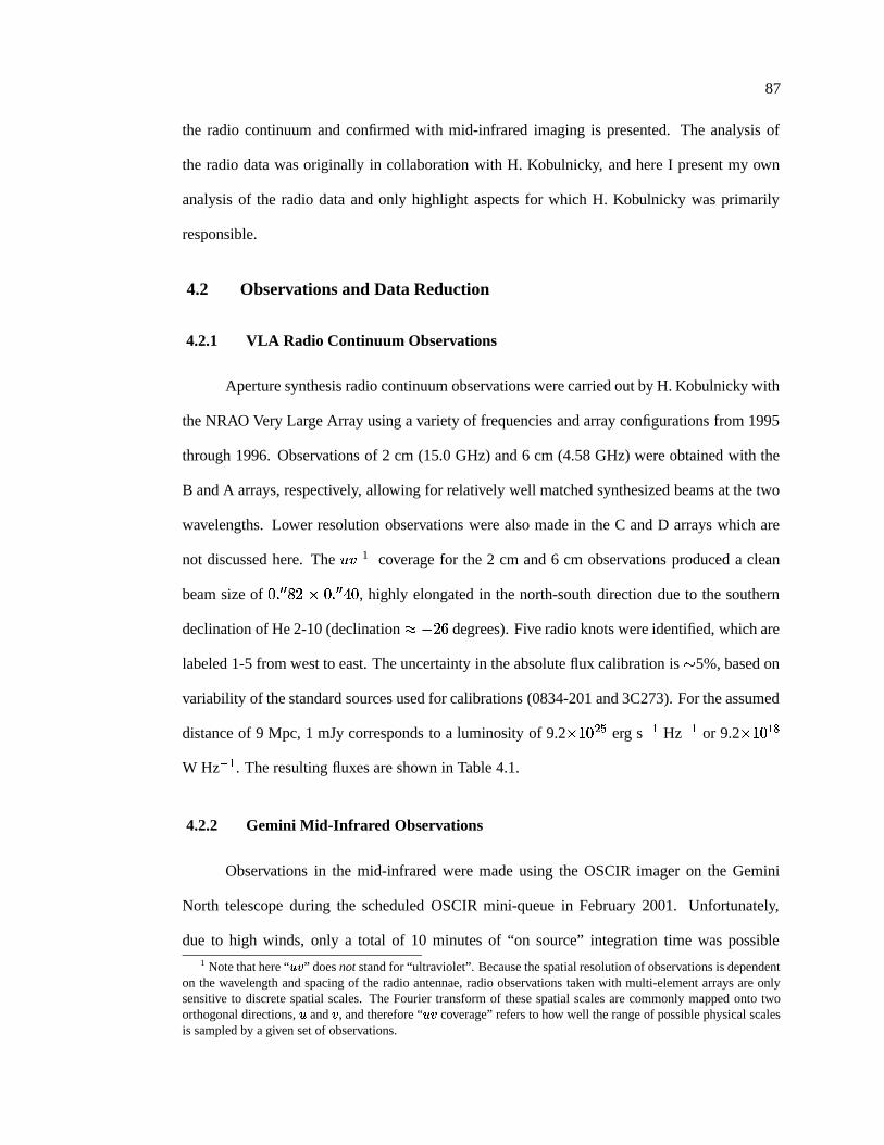
87
the radio continuum and confirmed with mid-infrared imaging is presented. The analysis of
the radio data was originally in collaboration with H. Kobulnicky, and here I present my own
analysis of the radio data and only highlight aspects for which H. Kobulnicky was primarily
responsible.
4.2 Observations and Data Reduction
4.2.1 VLA Radio Continuum Observations
Aperture synthesis radio continuum observations were carried out by H. Kobulnicky with
the NRAO Very Large Array using a variety of frequencies and array configurations from 1995
through 1996. Observations of 2 cm (15.0 GHz) and 6 cm (4.58 GHz) were obtained with the
B and A arrays, respectively, allowing for relatively well matched synthesized beams at the two
wavelengths. Lower resolution observations were also made in the C and D arrays which are
not discussed here. The � � 1 coverage for the 2 cm and 6 cm observations produced a clean
beam size of � � � � � � � � � � � � � , highly elongated in the north-south direction due to the southern
declination of He 2-10 (declination � � � � degrees). Five radio knots were identified, which are
labeled 1-5 from west to east. The uncertainty in the absolute flux calibration is � 5%, based on
variability of the standard sources used for calibrations (0834-201 and 3C273). For the assumed
distance of 9 Mpc, 1 mJy corresponds to a luminosity of 9.2� � � � � erg s ��� Hz ��� or 9.2
� � � � �
W Hz ��� . The resulting fluxes are shown in Table 4.1.
4.2.2 Gemini Mid-Infrared Observations
Observations in the mid-infrared were made using the OSCIR imager on the Gemini
North telescope during the scheduled OSCIR mini-queue in February 2001. Unfortunately,
due to high winds, only a total of 10 minutes of “on source” integration time was possible1 Note that here “ � � ” does not stand for “ultraviolet”. Because the spatial resolution of observations is dependent
on the wavelength and spacing of the radio antennae, radio observations taken with multi-element arrays are onlysensitive to discrete spatial scales. The Fourier transform of these spatial scales are commonly mapped onto twoorthogonal directions, � and � , and therefore “� � coverage” refers to how well the range of possible physical scalesis sampled by a given set of observations.
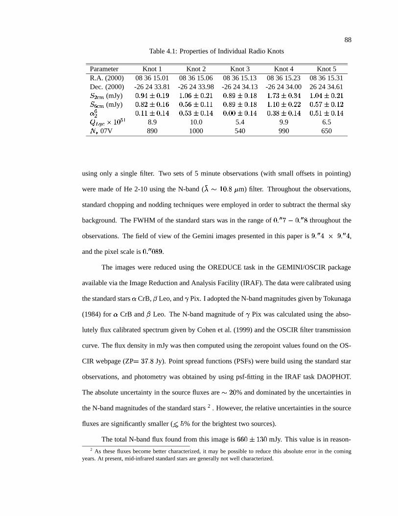
88
Table 4.1: Properties of Individual Radio Knots
Parameter Knot 1 Knot 2 Knot 3 Knot 4 Knot 5R.A. (2000) 08 36 15.01 08 36 15.06 08 36 15.13 08 36 15.23 08 36 15.31Dec. (2000) -26 24 33.81 -26 24 33.98 -26 24 34.13 -26 24 34.00 26 24 34.61�� � � (mJy) � � � � � � � � � � � � � � � � � � � � � � � � � � � � � � � � � � � � � � � � � � � � ��� � � (mJy) � � � � � � � � � � � � � � � � � � � � � � � � � � � � � � � � � � � � � � � � � � � � �� �� � � � � � � � � � � � � � � � � � � � � � � � � � � � � � � � � � � � � � � � � � � � � ���� ��
� � � � � 8.9 10.0 5.4 9.9 6.5���07V 890 1000 540 990 650
using only a single filter. Two sets of 5 minute observations (with small offsets in pointing)
were made of He 2-10 using the N-band ( �� � � � � � � m) filter. Throughout the observations,
standard chopping and nodding techniques were employed in order to subtract the thermal sky
background. The FWHM of the standard stars was in the range of � � � � � � � � � � � throughout the
observations. The field of view of the Gemini images presented in this paper is��� � � � �
�� � �
,
and the pixel scale is � � � � � � � .The images were reduced using the OREDUCE task in the GEMINI/OSCIR package
available via the Image Reduction and Analysis Facility (IRAF). The data were calibrated using
the standard stars � CrB,�
Leo, and Pix. I adopted the N-band magnitudes given by Tokunaga
(1984) for � CrB and�
Leo. The N-band magnitude of Pix was calculated using the abso-
lutely flux calibrated spectrum given by Cohen et al. (1999) and the OSCIR filter transmission
curve. The flux density in mJy was then computed using the zeropoint values found on the OS-
CIR webpage (ZP �� �� � Jy). Point spread functions (PSFs) were build using the standard star
observations, and photometry was obtained by using psf-fitting in the IRAF task DAOPHOT.
The absolute uncertainty in the source fluxes are � � � % and dominated by the uncertainties in
the N-band magnitudes of the standard stars 2 . However, the relative uncertainties in the source
fluxes are significantly smaller ( � � � % for the brightest two sources).
The total N-band flux found from this image is � � � � � � � mJy. This value is in reason-2 As these fluxes become better characterized, it may be possible to reduce this absolute error in the coming
years. At present, mid-infrared standard stars are generally not well characterized.
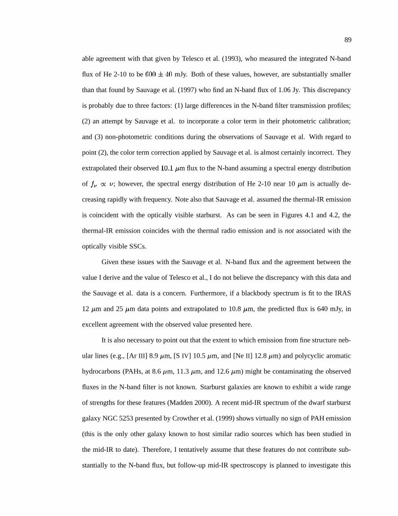
89
able agreement with that given by Telesco et al. (1993), who measured the integrated N-band
flux of He 2-10 to be � � � � � � mJy. Both of these values, however, are substantially smaller
than that found by Sauvage et al. (1997) who find an N-band flux of 1.06 Jy. This discrepancy
is probably due to three factors: (1) large differences in the N-band filter transmission profiles;
(2) an attempt by Sauvage et al. to incorporate a color term in their photometric calibration;
and (3) non-photometric conditions during the observations of Sauvage et al. With regard to
point (2), the color term correction applied by Sauvage et al. is almost certainly incorrect. They
extrapolated their observed � � � � � m flux to the N-band assuming a spectral energy distribution
of � � � � ; however, the spectral energy distribution of He 2-10 near 10 � m is actually de-
creasing rapidly with frequency. Note also that Sauvage et al. assumed the thermal-IR emission
is coincident with the optically visible starburst. As can be seen in Figures 4.1 and 4.2, the
thermal-IR emission coincides with the thermal radio emission and is not associated with the
optically visible SSCs.
Given these issues with the Sauvage et al. N-band flux and the agreement between the
value I derive and the value of Telesco et al., I do not believe the discrepancy with this data and
the Sauvage et al. data is a concern. Furthermore, if a blackbody spectrum is fit to the IRAS
12 � m and 25 � m data points and extrapolated to 10.8 � m, the predicted flux is 640 mJy, in
excellent agreement with the observed value presented here.
It is also necessary to point out that the extent to which emission from fine structure neb-
ular lines (e.g., [Ar III] 8.9 � m, [S IV] 10.5 � m, and [Ne II] 12.8 � m) and polycyclic aromatic
hydrocarbons (PAHs, at 8.6 � m, 11.3 � m, and 12.6 � m) might be contaminating the observed
fluxes in the N-band filter is not known. Starburst galaxies are known to exhibit a wide range
of strengths for these features (Madden 2000). A recent mid-IR spectrum of the dwarf starburst
galaxy NGC 5253 presented by Crowther et al. (1999) shows virtually no sign of PAH emission
(this is the only other galaxy known to host similar radio sources which has been studied in
the mid-IR to date). Therefore, I tentatively assume that these features do not contribute sub-
stantially to the N-band flux, but follow-up mid-IR spectroscopy is planned to investigate this
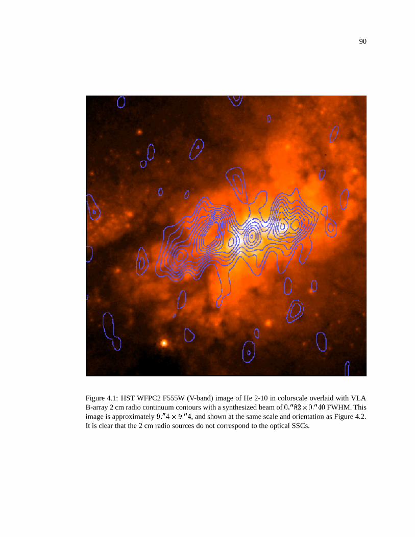
90
Figure 4.1: HST WFPC2 F555W (V-band) image of He 2-10 in colorscale overlaid with VLAB-array 2 cm radio continuum contours with a synthesized beam of � � � � � � � � � � � � � FWHM. Thisimage is approximately
��� � � � �
�� � �
, and shown at the same scale and orientation as Figure 4.2.It is clear that the 2 cm radio sources do not correspond to the optical SSCs.
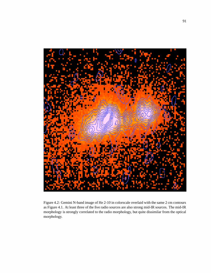
91
Figure 4.2: Gemini N-band image of He 2-10 in colorscale overlaid with the same 2 cm contoursas Figure 4.1. At least three of the five radio sources are also strong mid-IR sources. The mid-IRmorphology is strongly correlated to the radio morphology, but quite dissimilar from the opticalmorphology.
92
possibility.
The combined N-band flux of the three “detected” radio sources compared with the total
N-band flux of He 2-10 (as derived in this chapter, quoted in Telesco et al. 1993, or estimated
from the IRAS flux) suggests that at least � � � % of the 10.8 � m flux of the entire galaxy
can be attributed to only these three objects. Based on the relative morphologies of the diffuse
N-band flux seen in the Gemini image, is appears that very little of the remaining flux is due
to dust heated by the starburst component seen in the UV and optical bands. Most of the
diffuse background has a morphology similar to that of the radio sources, but on a larger scale.
Therefore, it is possible that some of this diffuse background flux in the N-band arises from
dust which is heated by radiation escaping from the embedded H II regions. If this is indeed the
case, then nearly all of the observed N-band flux, and by extension nearly all of the observed
flux from He 2-10 in the IRAS bands would be attributable to these enshrouded stellar clusters.
Given the vigorous recent star formation throughout He 2-10, as discussed in Chapter 3, this
result is rather remarkable.
4.3 Comparison of Optical, Radio, and Mid-IR Images
Figures 4.1 and 4.2 show the 2 cm radio contours overlaid on both the optical V-band
HST image (from Chapter 3) and the Gemini N-band image. The morphology of the radio
emission and the mid-IR emission are nearly identical. However, these images reveal a striking
dissimilarity between the optical morphology and that of the radio and mid-IR. Five radio knots
are apparent (labeled knots 1 through 5 from west to east), three (possibly four) of which are
also extremely bright N-band sources — knots #1, 4, and 5 are readily detected and #2 is likely
to be blended with #1 (the remaining radio source may also have mid-IR emission not detected
in the signal to noise allowed for in only the 10 minutes of integration time achieved).
The absolute coordinates of the radio map are accurate to � � � � � � , while the HST image are
uncertain by � � � � � � , limited by the positional uncertainties of the guide stars from the Guide
Star Catalog (Lasker et al. 1990). This leads to a relative positional uncertainty between the

93
radio and optical image of � � � � � � . Although there is a relative uncertainty of � � � � � between the
radio and optical image, there is no obvious correlation between the morphology 6-8 optical/UV
star clusters in the nuclear region of He 2-10 (distributed in a chevron configuration) and the
radio point sources. Given any possible � � � � � translation of the optical image, no more than 2
of the radio sources would have a corresponding optical counterpart. Given the high extinction
in the core of this galaxy, it is not surprising that the optical and radio morphologies are so
different.
4.4 The Nature of These Radio Sources
In order to determine the nature of these radio sources, let us first review the observational
constraints which must be satisfied. (1) There appear to be at least five such sources in He 2-10 at
sufficient signal to noise to be detected with these radio observations. (2) Each of these sources
has a positive spectral index ( � � � , where�
� � � � : higher fluxes at shorter wavelengths). (3)
The sources have 2 cm and 6 cm luminosities of � � � � � � � � � � � � erg s � � Hz � � . (4) Based on
a comparison with lower quality data from 1984 and 1985, these same radio sources are present
with the same fluxes (within the relative error) over roughly ten years. (5) These radio sources
each have corresponding 10 � m fluxes of � � � � mJy at 9 Mpc. With these constraints in mind,
possible types of radio sources can be put to the test.
4.4.1 Could These Objects be Supernovae Remnants?
Some of the most “conventional” radio objects are supernovae (SNe) and supernovae
remnants (SNR). He 2-10 has recently undergone a great deal of star formation (Chapter 3),
therefore it would be quite surprising if this galaxy were not prodigiously producing SNe. This
expected multiplicity easily passes criterion (1).
The first clue that these objects are not SNR is their positive spectral index; typical SNR
have � � � � � � , although not all SNR obey this “rule” — in particular, there is a class of
“composite” or “plerionic” SNR (as coined by Weiler & Panagia 1978) that are known to have
94
atypically flat spectral indices ( � � � � � � � � � � ). In fact, in the first few hundred days after
an SNe explosion, � can actually be positive (Weiler et al. 1986). Consequently, the positive
spectral indices of the radio objects in He 2-10 make it extremely unlikely that they could be
SNR, failing criterion (2). Since the radio fluxes of SNe have typical decay times of a few years
(Weiler et al. 1986), criterion (4) is almost certainly failed.
Criterion (5) is also failed by SNR. In the survey of Arendt (1989), he found that only
� 1/3 of SNR in the galaxy are even visible in the IRAS observations. The SNR which are
apparent in the IRAS observations have 12 � m fluxes which are almost exclusively less than
� � � Jy at galactic distances of � � � kpc. At the distance of He 2-10, these SNR would have
10 � m fluxes � � � mJy (two orders of magnitude fainter than the 10 � m fluxes observed for the
objects in He 2-10).
Finally, is it possible that these objects could be old SNR which are fading at a slower rate
than bright young SNR? The luminosities of typical SNR in the Milky Way are several orders
of magnitude less luminous, ranging from � � � � � � erg s � � Hz ��� for 1000 yr old remnants to
� � � � � � erg s ��� Hz � � for Cas A (330 yr old remnant). At the distance of He 2-10, a bright
young SNR like Cas A would be only a � � � detection in these observations, thus failing
criterion (3). In this case, 4 out of 5 observational criteria were failed, and SNR are ruled out as
a plausible origin for the radio objects in He 2-10.
4.4.2 Could These Objects be AGN?
Active galactic nuclei (AGN), such as radio loud quasars, can be quite luminous ra-
dio sources. From the sample of Kellermann et al. (1989), such quasars can be brighter than
� � � mJy at 6 cm, easily passing criterion (3). Some AGN are also known to have flat to slightly
positive spectral indices ( � � � � � � � , e.g., Nagar et al. 2000, although some of these “AGN” are
not conclusively ruled out as star forming nuclei). Therefore, criterion (2) is not necessarily
failed in this case. It is also not possible to rule out AGN based on criterion (4); while AGN are
known to have variations in their radio luminosities, these variations are not necessarily mono-
95
tonic. An AGN could very plausibly be observed at roughly the same luminosity in observations
separated by 10 years. The mid-infrared luminosities of AGN (dominated by the reprocess of
radiation in their dust tori) could also easily surpass criterion (5) (Urry & Padovani 1995).
Criterion (1) presents the real hurdle for AGN as candidates for the radio objects in He 2-
10. While in some galaxy mergers involving large spiral galaxies which each hosted its own
AGN, the young merger remnants may still have two discrete nuclei and therefore may also
contain two AGN. However, even a single AGN is unlikely to be found in a dwarf galaxy, and
five AGN in a single dwarf galaxy even more unlikely. As a result AGN are ruled out as a
possibility for the radio sources in He 2-10.
4.4.3 Could These Objects be Enshrouded H II Regions?
Compact H II regions are strong sources of free-free emission and represent most plau-
sible option for the origin of the radio sources in He 2-10. From Chapters 2 and 3, it is clear
that massive star clusters are formed in starburst galaxies such as He 2-10. If the star formation
in He 2-10 has been roughly continuous over the last 10 Myr, then for � � � SSCs formed in
this time period, we should expect � � SSCs to be formed every million years. Therefore, it
is entirely plausible that several radio sources attributable to SSC formation should be present,
and criterion (1) is easily passed.
Flat or positive spectral indices like the ones observed in He 2-10 are common for com-
pact H II regions in the Galaxy on sub parsec scales (e.g, see the compilation of Wood & Church-
well 1989a for ultra-compact H II regions, UCH IIs). This type of spectral energy distribution
is well understood in the case of UCH IIs as thermal bremsstrahlung emission which has a high
turnover frequency due to extremely high electron densities, thereby meeting criterion (2).
Criterion (3) could not be met by individual massive stars embedded in dense H II re-
gions, as is the case for UCH IIs, but rather would require several hundred massive stars to
create such luminous H II regions at radio wavelengths. However, this is exactly what one
should expect to observe when massive star clusters, such as SSCs, are early in their evolution.
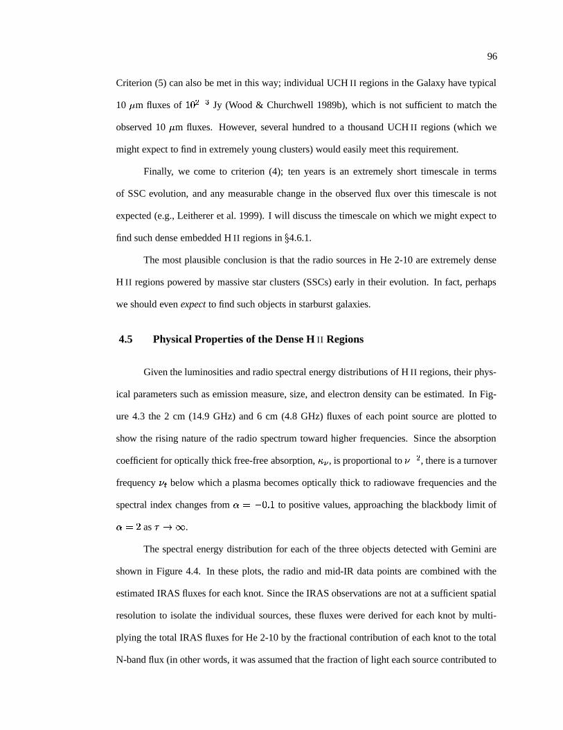
96
Criterion (5) can also be met in this way; individual UCH II regions in the Galaxy have typical
10 � m fluxes of � � � �� Jy (Wood & Churchwell 1989b), which is not sufficient to match the
observed 10 � m fluxes. However, several hundred to a thousand UCH II regions (which we
might expect to find in extremely young clusters) would easily meet this requirement.
Finally, we come to criterion (4); ten years is an extremely short timescale in terms
of SSC evolution, and any measurable change in the observed flux over this timescale is not
expected (e.g., Leitherer et al. 1999). I will discuss the timescale on which we might expect to
find such dense embedded H II regions in � 4.6.1.
The most plausible conclusion is that the radio sources in He 2-10 are extremely dense
H II regions powered by massive star clusters (SSCs) early in their evolution. In fact, perhaps
we should even expect to find such objects in starburst galaxies.
4.5 Physical Properties of the Dense H II Regions
Given the luminosities and radio spectral energy distributions of H II regions, their phys-
ical parameters such as emission measure, size, and electron density can be estimated. In Fig-
ure 4.3 the 2 cm (14.9 GHz) and 6 cm (4.8 GHz) fluxes of each point source are plotted to
show the rising nature of the radio spectrum toward higher frequencies. Since the absorption
coefficient for optically thick free-free absorption, � � , is proportional to � � � , there is a turnover
frequency � � below which a plasma becomes optically thick to radiowave frequencies and the
spectral index changes from � � � � � � to positive values, approaching the blackbody limit of
� � � as ����� .
The spectral energy distribution for each of the three objects detected with Gemini are
shown in Figure 4.4. In these plots, the radio and mid-IR data points are combined with the
estimated IRAS fluxes for each knot. Since the IRAS observations are not at a sufficient spatial
resolution to isolate the individual sources, these fluxes were derived for each knot by multi-
plying the total IRAS fluxes for He 2-10 by the fractional contribution of each knot to the total
N-band flux (in other words, it was assumed that the fraction of light each source contributed to
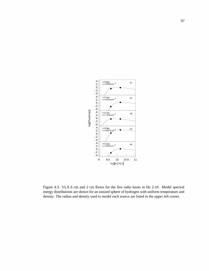
97
-.4-.2
0.2.4
#1r=3.3pc
-.4-.2
0.2.4
#2r=2.1pc
-.4-.2
0.2.4
#3r=4.7pc
log[
Flu
x(m
Jy)]
-.4-.2
0.2.4
#4r=3.0pc
9 9.5 10 10.5 11
-.4-.2
0.2.4
#5r=2.1pc
Figure 4.3: VLA 6 cm and 2 cm fluxes for the five radio knots in He 2-10. Model spectralenergy distributions are shown for an ionized sphere of hydrogen with uniform temperature anddensity. The radius and density used to model each source are listed in the upper left corner.
98
the N-band will be the same relative fraction in the IRAS observations). These spectral energy
distributions bear a remarkable resemblance to those for ultracompact H II regions (e.g., Wood
& Churchwell 1989b).
4.5.1 Emission Measures
Using the analytical approximation of Mezger & Henderson (1967), the emission mea-
sure,� � � �
� �� � � , can be estimated given an electron temperature, � , the observing fre-
quency, � , and the optical depth at that frequency, � .
� � � � � � � ��� � � � � � ��� ���� � � � � � � �
� ����� � � � � � � (4.1)
The positive spectral index for these sources arises from free-free emission where � � ��� ,therefore I assume � � � as a lower limit. Adopting � � =6000 K based on the spectroscopy of
Kobulnicky et al. (1999), the resulting emission measures are in excess of � � � � � � cm � pc at
6 cm (for � ��� these emission measures will be correspondingly higher).
4.5.2 Comparison With Model H II Regions
In order to better constrain the properties of these sources, I have created model H II
regions (spherical, uniform electron density and electron temperature) of radius, , electron
temperature, ��� , and electron density, � � . Only free-free emission and absorption processes are
considered, and a temperature of 6000 K is assumed, based on the work of Kobulnicky et al.
(1999). The models are somewhat insensitive to variation in temperature in a reasonable range
about this value; since the optical depth goes as � � � �� � � , the main effect of changing the
assumed temperature is to shift the turnover frequency. For a reasonable range in temperatures
(e.g., 5000 - 8000 K), the turnover frequency could only shift by � � � � � GHz.
In Figure 4.3 the resulting spectral energy distributions are shown for a range of models.
The luminosities and spectral indices of these compact sources are well-fit by model H II regions
with a radius of 2—5 pc, and electron densities of 1400-5400 cm � � at a distance of 9 Mpc. In
99
-1 -2 -3 -4 -5
0
1
2
3
4 UDHII #1
UDHII #4UDHII #5
log[
F(m
Jy)]
Figure 4.4: The spectral energy distribution of the UDH IIs in He 2-10. The 12 � m, 25 � m,60 � m, and 100 � m have been estimated by multiplying the total IRAS flux of He 2-10 by thefractional percentage of the total N-band flux for each UDH II.
100
reality, we might expect that the radio structures are not single monolithic H II regions, but a
collection of smaller H II regions with higher densities embedded in a lower density medium,
however this picture is not yet clear.
4.5.3 Limits on the Contribution From SNe
In � 4.4 it was clear that these radio sources could not be SNe or SNR, but rather are most
likely to be embedded H II regions. Never the less, it is possible that non-thermal flux from SNe
and SNR might be contributing to the observed fluxes. The lowest frequency observed (in this
case 4.58 GHz) can be used to place an upper limit on both the SN frequency and the fraction of
the highest frequency flux (in this case 15 GHz) which might be due to non-thermal emission.
In order to make these estimates, it is necessary to examine the case, as an upper limit, that
all of the 4.8 GHz flux is due to synchrotron radiation. The maximum amount of non-thermal
emission at 15 GHz is given by,
�� �� ������� � � � ����
� � � ������� � � � � �� ��� � (4.2)
Adopting � � � � � � (typical of synchrotron sources in the Galaxy, Condon 1992), the max-
imum amount of non-thermal flux which could be contaminating the 15 GHz observations is
� � � � � � � � �� ��� .
Following Condon & Yin (1990) and Condon (1992), the SN frequency can also be
constrained. The relation between the SN frequency and non-thermal luminosity is given by,
� � ��� � � ��� �� � � � � ��� � � � � � � �
������� � � � � ���� ��� � � (4.3)
As an example using knot 4 (the brightest knot in this sample), and again adopting � � � � � �
(Condon 1992), the maximal SN frequency is given by ��� � � � � � � � � � yr � � . Using the
Starburst99 models of Leitherer et al. (1999), this SN frequency is almost an order of magnitude
less that the SN frequency expected when SN begin to occur at an age of � � Myr for a model
cluster. Therefore, it is unlikely that SNe have begun to occur in significant numbers, if at
101
all, and we expect the non-thermal contamination in these data to be insignificant. Moreover,
the paucity of SNe puts an absolute upper limit on the ages of these clusters of � �Myr
(although, as we will see in � 4.6.1 the ages can be constrained to much younger values with
other methods).
4.5.4 Ionizing Radiation
The production rate of Lyman continuum photons, and thus the stellar content of each
of the embedded H II regions can be estimated from the thermal radio luminosity following
Condon (1992),
��� ��� � � � � � � � � � ��� � � �
� � � � � � � � � �
� ��� � � � � � � � � � � � �
� � � ��� � � � ��� ��� � � � � (4.4)
Since the non-thermal component becomes weaker at higher frequencies, the luminosity mea-
sured at the highest radio frequency (in this case 15 GHz) is used to determine� � �
� . The
resulting values determined from this method are presented in Table 4.1.
One should also bear in mind that the��� �
� values determined with this method could
suffer from two different problems: (1) if the source is, in fact, optically thick even at the
highest frequency measured, this method will underestimate the actual ionizing luminosity, and
(2) if there is contamination from non-thermal emission in the beam at the frequency used, the
ionizing luminosity will be overestimated. However, the overall non-thermal background of the
galaxy will tend to be resolved out with the small synthesized beams used in these observations.
Therefore the only non-thermal flux which might boost the 15 GHz luminosity would be SNe
within the objects themselves. I estimate the maximum affect this might have in � 4.5.3, and do
not expect any significant contribution.
Further evidence for deriving the ionizing luminosity from this method comes by com-
paring the total��� �
� calculated for He 2-10 using the 15 GHz flux with the total� � �
� calcu-
lated from optical H � observations;��� �
� determined in the radio should include the ionizing
flux apparent in optical light, the ionizing flux which is optically obscured, and any non-thermal
102
contamination. As a result, if there is non-thermal contamination, the radio� � �
� cannot be less
than the optically determined��� �
� . Conversely, if the radio��� �
� is less than the optically
determined��� �
� that implies that the radio value is underestimating the ionizing luminosity.
Kobulnicky & Johnson (1999) find��� �
�� � � � � � � � � s � � for the entire galaxy using the
15 GHz luminosity. The Mendez et al. (1999) H � measurement yields� � �
�� � � � � � � � � s ��� ,
which is only marginally larger than the value determined in the radio. Therefore, I conclude
that non-thermal contamination is not significantly contributing to the 15 GHz flux, and this
method for deriving��� �
� will not be an overestimation, but rather is quite possibly an underes-
timation.
4.5.5 Stellar Content
The production rate of Lyman continuum photons from these sources can be used to
estimate the number of massive stars powering the observed emission. Following the convention
of Vacca (1994) and Vacca et al. (1996), a “typical” O-star (type O7V) produces� � �
�� � � � �
� � � �
s � � . Using this method, 20,000 such O stars are required to power the total observed
radio ionizing luminosity from He 2-10. Each of the individual embedded clusters require
between 500 and 1000 equivalent O7V stars in order to produce their ionizing luminosities (see
Table 4.1). Thus, each embedded cluster contains more O stars than are found in the entire
30-Doradus nebula in the LMC ( � � � � , Vacca et al. 1995). Using the Starburst99 models of
Leitherer et al. (1999) with solar metallicity, Salpeter IMF, an upper mass cutoff of 100 M ,
and a lower mass cutoff of 1 M , starburst knots producing this range of Lyman continuum
photons at an age of 1 Myr would have masses of 0.8 - 1.6� � � � M (if the lower mass cutoff
is � � M , these mass estimates will be correspondingly higher). These masses are consistent
with those found for the optical SSCs in He 2-10 (Chapter 3) which have already emerged from
their birth material, thus strengthening the connection between UDH IIs and SSCs.
Since the star-forming regions seen in these radio observations are not seen even faintly
on the HST V- or I-band images (or even in the near-infrared, Vacca et al. in preparation), their
103
visual extinctions must be quite large. Such large extinction values are consistent with the col-
umn density of molecular gas observed in this region (Kobulnicky et al. 1995) and the extinction
estimates from the infrared silicate features (� �
�� � , Phillips et al. 1984). Given that He 2-10
was already known to contain 31,000 O stars (Conti & Vacca 1994) the additional � 4000 O
stars contained in these five dense, heavily obscured H II regions represent a significant faction
of the massive stars in He 2-10.
4.6 Discussion
The major result of this chapter is the discovery of multiple optically thick free-free
sources, most plausibly dense H II regions powered by extremely young embedded massive star
clusters. The majority of these sources do not coincide with features visible in the optical HST
images, leading to the conclusion that they are heavily obscured by dust. The combination of
high obscuration and high density inferred from the free-free optical depth is consistent with
very dense H II regions. While such dense, optically-thick, inverted-spectrum H II regions exist
in abundance around individual stars in the Galaxy (i.e., ultracompact H II regions; Wood &
Churchwell 1989b) this phenomenon had not been previously seen on such large spatial and
energetic scales. Because of their similar densities to ultracompact H II regions in the Galaxy,
we might term them “ultra dense H II regions” (UDH IIs).
4.6.1 On the Lifetimes of UDH IIs
If UDH IIs are similar to (albeit vastly scaled up) from UCH IIs, it seems likely that the
fraction of time a super star cluster spends in the UDH II phase is a small fraction of the massive
star lifetime. In accord with the estimated lifetimes of individual UCH II regions based on the
number of UCH II regions compared with the number of optically visible O stars in the Galaxy
(e.g., Wood & Churchwell 1989a) is � � � � � � %. Indeed, UCH II region lifetimes have been a
topic of much discussion since Wood & Churchwell (1989b) introduced the “lifetime problem”;
in short, if UCH II regions are significantly overpressured with respect to the surrounding ISM,
104
they should expand and dissipate on time scales � � � � years. However, the number of UCH II
regions observed is greater than is allowed for by this time scale.
Several mechanisms have been proposed to address this issue, most of which are also
likely to be applicable to UDH IIs. Wood & Churchwell (1989b) proposed that infalling matter
or bow shocks might act to increase the external pressure, thus extending the UCH II phase. It
is also possible that the ambient pressure is typically significantly higher than the value used by
Wood & Churchwell (1989b), as proposed by de Pree et al. (1995). The lifetimes of UCH II
regions could also be extended if they are replenished by material photoevaporated from the
surrounding circumstellar disks (e.g., Hollenbach et al. 1994).
The first argument for the extreme youth of UDH II regions is simply by analogy to
UCH II regions in the Galaxy. If UDH IIs are composed of individual UCH II regions, we
should expect them to have similar lifetimes provided that star formation is relatively instanta-
neous over the massive star cluster. As is the case for UCH II regions, the densities in UDH IIs
are likely to be extremely high, and the implied pressures constitute an over-pressure compared
to typical ISM pressures. If the surrounding ISM has typical densities of ��� � � � � cm �� ,then these embedded H II regions with densities of � � � � � � � cm � � are at an overpressure of
� � � . To first order, such over-pressed regions must rapidly expand and disperse on time scales
comparable to the sound-crossing time scale which is a few� � � � years for � � � � � km s ��� .
However, as discussed above for UCH II regions, it is entirely possible that the ambient pressure
around UDH IIs is not “typical” of the global ISM and might present a mechanism for extending
the lifetime of the UDH II phase.
The second method to estimate the lifetimes of UDH IIs is to compare the fraction of
ionizing stars in UDH II regions with the total number of ionizing stars in the galaxy. The
total Lyman continuum photon production rate,��� �
� , of the UDH II regions in He 2-10 is
��� � � � � � s � � (provided there is no leakage from the enshrouding cocoon that would likely
result in associated H � emission). The��� �
� determined optically for the entire galaxy He 2-10
is � � � � � � � � s � � (Mendez et al. 1999), implying a total� � �
�� � � � � � � � � s ��� . Thus, the UDH II
105
regions contain � � � � � the total ionizing photons. It then follows that if the star formation has
been reasonably continuous in this system over the last 10 Myr, a plausible estimate for the
typical duration of the UDH II phase is � � � % times the typical massive star lifetime (� � � �
yr), remarkably in accord with the estimates for individual UCH II regions. This method implies
a mean lifetime of roughly 1 – 2 Myr for UDH II regions, although if strong star formation has
been occurring over less than 10 Myr, this estimate will be correspondingly lower. A similar
method to estimate the lifetimes of UDH IIs is simply to compare the number of clusters which
are no longer enshrouded ( � � � from Chapter 3) to the number of UDH IIs. Given that the
optical clusters in He 2-10 are typically less than 10 Myr old, this method implies the UDH II
phase only lasts a few� � � � years, which is slightly lower than the lifetimes estimated with the
first method. While these estimates are very crude, a reasonable lifetime for the UDH II phase
is perhaps � ��� Myr.
Perhaps the weakest argument in favor of the extreme youth of UDH II regions comes
from their high visual extinctions. In � 4.3 it is clear that the UDH II regions are not visible at
optical wavelengths. This picture is consistent with UDH IIs being extremely young H II re-
gions still hidden from view by the dust associated with their natal molecular clouds. However,
one must also bear in mind that we cannot rule out screens of dust not physically associated
with the regions of optically thick free-free emission.
4.6.2 UDH IIs in Other Starburst Systems?
It would be quite surprising if the UDH II phenomenon was unique to He 2-10. If
UDH IIs do indeed represent the early stages of SSCs evolution, then they ought to be present
in most (if not all) starburst galaxies. High resolution 2 cm and 6 cm radio observations of a
large sample of starburst systems acquired in scaled B and A-array configurations with the VLA
will be required to examine this issue. To date, such high spatial resolution data generally exist
only for more luminous systems like quasars and AGN. In some cases (as will be discussed in
the following chapter) perhaps other star-forming galaxies contain dense, heavily obscured H II
106
regions like the five in He 2-10, but they have simply not been identified as such. Never the less,
very little data currently exists which can adequately address the ubiquity of UDH IIs, and this
area of research will benefit from an extensive observing campaign.
Turner et al. (2000) detected one such object in the nucleus of the galaxy NGC 5253.
NGC 5253 is a dwarf starburst galaxy in the Centaurus group of galaxies at a distance of ��� � Mpc (Sandage et al. 1994). The radio object in NGC 5253 has estimated properties which
are fully consistent with it being a genuine UDH II. In fact, follow-up work by Gorjian et al.
(2001) has also confirmed this UDH II with mid-IR Keck observations. Turner et al. estimate
that this object has a radius of � � pc, and has an ionizing photon rate of� � �
�� � � � � � � � s ��� ,
in close agreement with the results of this chapter. My own analysis of this system, using the
2 cm fluxes from Turner et al. (1998) and the 1.3 cm fluxes from Turner et al. (2000), indicate a
best-fit radius of 3.6 pc and an electron density of � � � � � � � cm � � (Figure 4.5) for an electron
temperature of 11,000 K (as derived by Kobulnicky et al. 1997). These values are remarkably
close to the electron densities and radii found for the UDH IIs in He 2-10 in � 4.5.2.
Arguably the most well known starburst in the local universe is M 82, making it an
obvious object for comparison. With a distance of only � 3.6 Mpc (Freedman et al. 1994), it
can be studied at higher spatial resolution than He 2-10. Radio continuum maps presented in
Allen & Kronberg (1998) show 26 compact sources with linear diameters of 3.5 pc ( � � � � � ) and
2 cm spectral luminosities of 2.9� � � � � erg s � � Hz ��� to 7.3
� � � � � erg s ��� Hz � � (fluxes of 0.2
mJy to 5 mJy). Of the 26 sources in M 82, 22 show distinctly non-thermal spectral indices
and are consistent with supernova remnants. Their radio spectra often show turnovers, but only
at low frequencies ( � ��� GHz), due to free-free absorption in the surrounding ionized gas.
Only one source has a thermal spectrum typical of an H II region, but it is quite flat with no
indication of a turnover due to free-free absorption. de Grijs et al. (2001) suggest that M 82
has possibly undergone several starburst episodes and hosts sites of “fossil” starbursts. Perhaps
M 82 is between starburst events, or even possibly post-starburst, and therefore not producing
UDH IIs in large numbers.
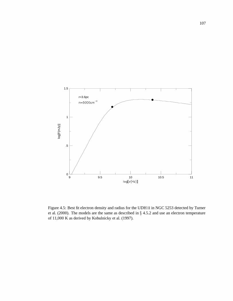
107
9 9.5 10 10.5 110
.5
1
1.5
log[
F(m
Jy)]
r=3.6pc
Figure 4.5: Best fit electron density and radius for the UDH II in NGC 5253 detected by Turneret al. (2000). The models are the same as described in � 4.5.2 and use an electron temperatureof 11,000 K as derived by Kobulnicky et al. (1997).
108
4.6.3 Implications for the Infrared-Radio Correlation?
There is a well-known correlation between the infrared and radio fluxes of galaxies over
a wide range of Hubble types as first reported by van der Kruit (1971). This relation is typically
represented by the logarithmic far-infrared(FIR)-to-radio flux ratio
����� � ��� � � � � � � � � � � � � � ��� � � � � �� ��� � � (4.5)
where � � � is an approximation of the flux between � � � and � � � � � m as
� � � � � � � � � � � � � � � � � � � � � � � � � � � � � �� �
� � � � � � � (4.6)
where�� � �� ��� , � � � � � , and
�� � � � � are the flux densities (in units of W m � Hz ��� ) at 1.49 GHz,
60 � m, and 100� m, respectively.
Over a range of spiral, irregular, and starburst galaxies (see Sanders & Mirabel 1996, and
references therein), � is very robust with a small standard deviation;� � � � � � � � � � � � . 3 For
starbursts selected from the IRAS Bright Galaxy Survey, Condon et al. (1991b) find an average
value of � � � � � � � � � � � . They also find � tends to be higher for the more infrared lumi-
nous galaxies. Furthermore, these galaxies with high � values also tend to have compact radio
sources. Condon et al. hypothesize that this class of ultraluminous infrared galaxies (ULIGs)
are powered by dense, compact starbursts which are optically thick at 1.49 GHz, and whose
radio flux density is therefore suppressed relative to the FIR. Correcting for the optical depth at
1.49 GHz yields a tighter FIR-radio correlation.
In the extreme case that a galaxy were entirely in the UCH II/UDH II phase, what would
its � value be? To answer this question, let us use W49A as an analogy. W49A is one of the most
well-studied UCH II complexes in the Galaxy and has been resolved into at least 30 UCH IIs (de
Pree et al. 1997). From the Ward-Thompson & Robson (1990) values for�� � � � and
�� � � � � ,
� � � � � � � � � � � �
W m � � for W49A. From Mezger et al. (1967), � (1.41 GHz) �� � � �
Jy.3 Notable exceptions to this correlation are radio galaxies and radio-loud QSOs, which have � values typically
lower by a factor of ������ (see Sanders & Mirabel (1996) and references therein).
109
These values yield � � ��� � , which is significantly higher than the average value found in
normal galaxies and starbursts, and even higher than the typical � values obtained for ULIRGs.
Given the high � value derived above for W49A, which is entirely dominated by ex-
tremely young and embedded massive stars, we might also expect to find a high � value for
the galaxies in which we have detected UDH IIs. Using the IRAS Point Source Catalog fluxes,
we find that He 2-10 has � � � � � � � � � � � ��� � W m � � and NGC 5253 has � � � � � � � � �
� � � � � W m ��� . From Kobulnicky & Johnson (1999), � (1.42 GHz) �� � � �
mJy for He 2-10,
and from Turner et al. (1998) � (1.49 GHz) �� � � � mJy for NGC 5253. The resulting � values
are 2.63 and 2.69 for He 2-10 and NGC 5253, respectively, and are both significantly higher
than the average value derived for starburst galaxies, but consistent with the typical value of
ULIRGs. Even after correcting the radio flux from He 2-10 for self-absorption according to the
prescription given by Condon et al. (1991b), � is still significantly higher than the canonical
value with the corrected value of � � � � � .The most straightforward interpretation is that bulk of the star formation in He 2-10 is so
young that it has not yet begun to produce SNe in the relative numbers typical in most galaxies,
in agreement with the result for the embedded clusters in � 4.5.3. In other words, while the
five embedded clusters in He 2-10 are largely (or solely) responsible for the mid- to far-infrared
flux, they are not yet mature enough to produce synchrotron radiation in amounts necessary to
obtain the standard � value.
How does the � value of the nearby starburst M82 (where there currently don’t appear
to any UDH IIs) compare? From Kuehr et al. (1981), the 1.4 GHz flux of M82 is 8.6 Jy, and
from Soifer et al. (1989) values for the 100 � m and 60 � m fluxes are 1355 Jy and 1313 Jy,
respectively. I calculate �� � � � � � � � � � ��� � , which results in � � � � � � . This � value is
in excellent agreement with those derived for other galaxies by Condon et al. (1991b), but
significantly lower than the values derived above for He 2-10 and NGC 5253, both of which are
known to host UDH IIs, while M82 does not.
Although we have a sample size of only two galaxies hosting UDH IIs, they both have
110
� � � � � , while the local starburst M82 which does not host UDH IIs have a � value significantly
lower. This trend is exactly what we would expect for galaxies undergoing vigorous star forma-
tion and hosting massive UDH IIs. This tentative result lends itself two main implications: (1)
� values might be useful for identifying galaxies which are most likely to host UDH IIs, and (2)
because high � values are typical of ULIRGs, UDH IIs might have a significant role in powering
their infrared luminosities.
Chapter 5
A Sample of Clusters of Extragalactic Ultracompact H II Regions
5.1 Background
In the previous chapter I discussed the discovery of very young massive star clusters still
embedded in their birth material in He 2-10. Subsequently, a handful of other such objects have
also appeared in the literature in NGC 5253 (Turner et al. 2000), NGC 2146 (Tarchi et al. 2000),
and NGC 4214 (Beck et al. 2000). Embedded in these heavily enshrouded objects are hundreds
of young massive stars that create surrounding H II regions and manifest themselves as optically
thick free-free radio sources.
Similar dense, inverted-spectrum H II regions exist around individual stars in our galaxy
(i.e., ultracompact H II regions, UCH IIs, Wood & Churchwell 1989), albeit on a vastly smaller
scale. Because of their apparent spectral similarity to galactic UCH IIs, we have dubbed these
extragalactic objects “ultradense H II regions” (UDH IIs). The physical properties of these clus-
ters are truly remarkable; the estimated sizes (a few parsecs), stellar masses (a few� � � � � � ),
ionizing luminosities (��� �
�� � � � � � � � s ��� ), and ages (possibly as young as a few
� � � � years)
of the newly discovered UDH IIs imply that we may be witnessing the birth process of super
star clusters, and therefore possibly the genesis of globular clusters. The discovery of these
UDH IIs allows us to begin observing the earliest stages of the massive star cluster formation
for the first time. Moreover, if UDH IIs are indeed scaled-up versions of individual UCH II
regions, then perhaps we ought to find a continuous range of embedded cluster sizes, spanning
the gap between a single O-type star and a thousand or more O-type stars.
112
We have made some progress understanding the early stages of massive star evolution
in the Galaxy, but the current knowledge about the early stages of massive star evolution in
other environments is mediocre at best. The present state of the research on the early stages
of massive star evolution now includes both individual massive stars in the Galaxy (UCH II
regions) and massive star clusters in a handful of other systems (UDH IIs, Chapters 4 and 5).
However, little is known about individual massive stars in other galaxy systems. Perhaps the
most logical place to study individual massive stars early in their evolution is in the galaxies
closest to our own, the Large and Small Magellanic Clouds. However, data with sufficient
angular resolution to disentangle individual massive stars in the Magellanic Clouds is not yet
available. Despite this instrumental contraint, it is still possible to find “candidate” UCH IIs
even with large-beam data. In Appendix A, I present the results of a search for UCH II region
candidates in the Magellanic Clouds using previously published radio data in combination with
sources cataloged by IRAS. The large beamsizes in these surveys do not allow us to accurately
estimate the physical properties of these candidate UCH II regions; however I include this list
for completeness.
Because UDH IIs have only recently been identified, one of the primary goals in this
new field of study is simply to expand the sample of known objects in order to understand
their properties in a statistical sense. To this end, I have searched for previously published
radio observations that may have also serendipitously detected UDH IIs. Multiwavelength radio
observations taken to study supernovae remnants in nearby galaxies are particularly useful for
this purpose. In most cases, the original authors have identified the candidate UDH IIs I present
here as “thermal sources” or “H II regions.” I seek sources with positive radio spectral indices
( � ��� , where�
� � � � ), implying an optically thick free-free origin. In this chapter, I utilize
previously published radio observations of M33, NGC 253, and NGC 6946 to identify new
candidate UDH IIs, determine their number of ionizing stars, and estimate their physical sizes,
densities, and masses.
113
5.2 Galaxies in This Sample
Here I overview basic properties of the galaxies in this sample and only highlight the
radio observations utilized in this paper. I refer the reader to the original papers for more detail
on the observations and reduction. Because the observations were compiled from a variety
of sources, the observations are heterogeneous in nature, and in some cases, non-ideal for my
purposes. For example, in order to obtain accurate relative fluxes at multiple frequencies it is
desirable to have well-matched beam sizes; I will discuss the impact of mismatched beams in
� 5.3.1. However, these data provide a valuable resource for this fledgling field and will serve
as a useful baseline for follow-up observations.
5.2.1 M33
M33 (NGC 598) is a Local Group spiral galaxy (Sc(s)II-III), nearly face-on (� � � � �
,
Garcia-Gomez & Athanassoula 1991), and it is rich in H II regions (Hodge et al. 1999; Courtes
et al. 1987; Boulesteix et al. 1974). Young ( � � � �
yr) clusters in M33 were recently studied
by Chandar et al. (1999), and were found to have masses of � � � � � � � � � � � M , smaller
than that typical for its old globular clusters. M33 has an areal star formation rate of SFR �
� � ��� � � M yr ��� kpc ��� (Kennicutt 1998), making it the least prolific galaxy in this sample. At
a distance of 840 kpc (Freedman et al. 1991), it is also the closest of the galaxies in this chapter.
The radio observations of M33 that I use were originally obtained by Duric et al. (1993)
and also presented by Gordon et al. (1999). Both Very Large Array (VLA) B configuration
and Westerbork Synthesis Radio Telescope (WSRT) observations were made of M33 at 6 and
20 cm (4.84 and 1.42 GHz) in several pointings to obtain good coverage of the galaxy. The
primary beams at 20 cm were� � � with the VLA and
� � � with WSRT. At 6 cm both telescopes
had primary beams of� �
. The 6 cm observations had resolutions ranging from � � � to � � � � , and
the 20 cm observations had resolutions ranging from � � � to � � � � , depending on the uv taper used
in the cleaning process. Matched beam observations were convolved to identical beams of� � �
114
FWHM. All images have an average 3 � rms noise level of � � � � � Jy per beam. At the adopted
distance of 840 kpc (Freedman et al. 1991), 1 Jy � � �� � � � � � erg s � � Hz � � .
5.2.2 NGC 253
At 2.5 Mpc (Turner & Ho 1985), NGC 253 is a member of the Sculptor Group. This
galaxy is a nearly edge-on spiral galaxy (Sc(s)), and contains a radio continuum plume em-
anating from the central starburst region rising perpendicular to the disk (e.g., Carilli et al.
1992). NGC 253 has the highest star formation rate of the galaxies in this sample with SFR �
� � � � � M yr ��� kpc ��� (Kennicutt 1998). Four young SSCs were discovered optically in the
central region of NGC 253 by Watson et al. (1996); however, only one of these clusters is
apparent in the mid-IR observations of Keto et al. (1999), who propose that it might be excep-
tionally young. Ulvestad & Antonucci (1997) also discuss the nature of the brightest thermal
radio source in NGC 253, a point that I will revisit in � 5.3.
NGC 253 was observed by Ulvestad & Antonucci (1997) with the B configuration of the
VLA at 1.3 cm, 2 cm, 3.6 cm, 6 cm, and 20 cm (23.56 GHz, 14.94 GHz, 8.44 GHz, 4.86 GHz,
and 1.49 GHz) between 1987 and 1995. Additional observations at 1.3 and 2 cm were made
using the A configuration. As the beam sizes at 6 and 20 cm are significantly larger than at
1.3 cm, 2 cm, and 3.6 cm, I have not included this longer wavelength data in my analysis
because of the unwanted background contribution from non-thermal emission. The duration of
the observations in the B-array were 4.1, 5.6, and 7.0 hours at 1.3, 2, and 3.6 cm, respectively.
The A-array observations at 1.3 and 2 cm were 2.8 and 4.2 hours, respectively. The primary
beams varied from � � to ��
(from 1.3 cm to 3.6 cm, respectively) and easily contain the area
of interest. The synthesized beams ranged from � � � � � � � � � � � � � to � � � � � � � � � � � � � at 1.3 cm,
� � � � � � � � � � � � � to � � � � � � � � � � � � � at 2 cm, and � � � � � � � � � � � � � to � � � � � � � � � � � � � at 3.6 cm. Ulvestad
& Antonucci (1997) estimate the uncertainties in these data as � � � % for 1.3 cm, and � � � %for the 2 cm and 3.6 cm data. The 3 � rms noise levels are � 660, 240, and 150 � Jy, respectively,
for the 1.3 cm, 2 cm, and 3.6 cm data. At the adopted distance of 2.5 Mpc (Turner & Ho 1985),
115
1 Jy ��� � � � � � � erg s ��� Hz � � .
5.2.3 NGC 6946
NGC 6946 is the most distant galaxy in this sample at 5.1 Mpc 1 (de Vaucouleurs 1979),
and is a spiral galaxy of type Sc(s)II with an inclination angle of� � � � �
(Garcia-Gomez &
Athanassoula 1991). The areal star formation rate in NGC 6946 is SFR � � � � � � �
M yr ��� kpc � �(Kennicutt 1998). Larsen & Richtler (1999) have detected 107 young massive star clusters,
one of which has received particular attention because of its age ( � � � Myr) and mass ( �
� � � � � M ) (Elmegreen et al. 2000b). Sub-mm images obtained by Bianchi et al. (2000) show
850 � m emission which, in some cases, may be associated with radio sources discussed in this
here.
The VLA was used to survey NGC 6946 with the B and A arrays at 6 and 20 cm (4.86
and 1.45 GHz), respectively, by Lacey et al. (1997). Approximately 8.6 hours were spent in
at each frequency. The primary beams were� �
and� � � at 6 cm and 20 cm, respectively. The
resulting beam sizes at the two wavelengths are very well matched: � � � � � � � � � � � at 6 cm and
� � � � � � � � � � � at 20 cm. Flux uncertainties are typically � � � %, and the 3 � rms noise levels are
� 60 and 50 � Jy for the 20 and 6 cm data, respectively. At the adopted distance of 5.1 Mpc (de
Vaucouleurs et al. 1976), 1 Jy ��� � � � � � �
erg s ��� Hz ��� . These observations have also been
analyzed by Hyman et al. (2000), who derive a luminosity function for H II region candidates
with a power-law index at 6 cm of � � � � � , but exclude sources with spectral indices of � � � � � .As result, the most optically thick sources were excluded from their sample. Nevertheless, the
seven sources presented in Hyman et al. (2000) with � � � are also included in this chapter
(my sources 1, 2, 4, 6, 7, 8, and 10 in Tables 5.3 and 5.6).
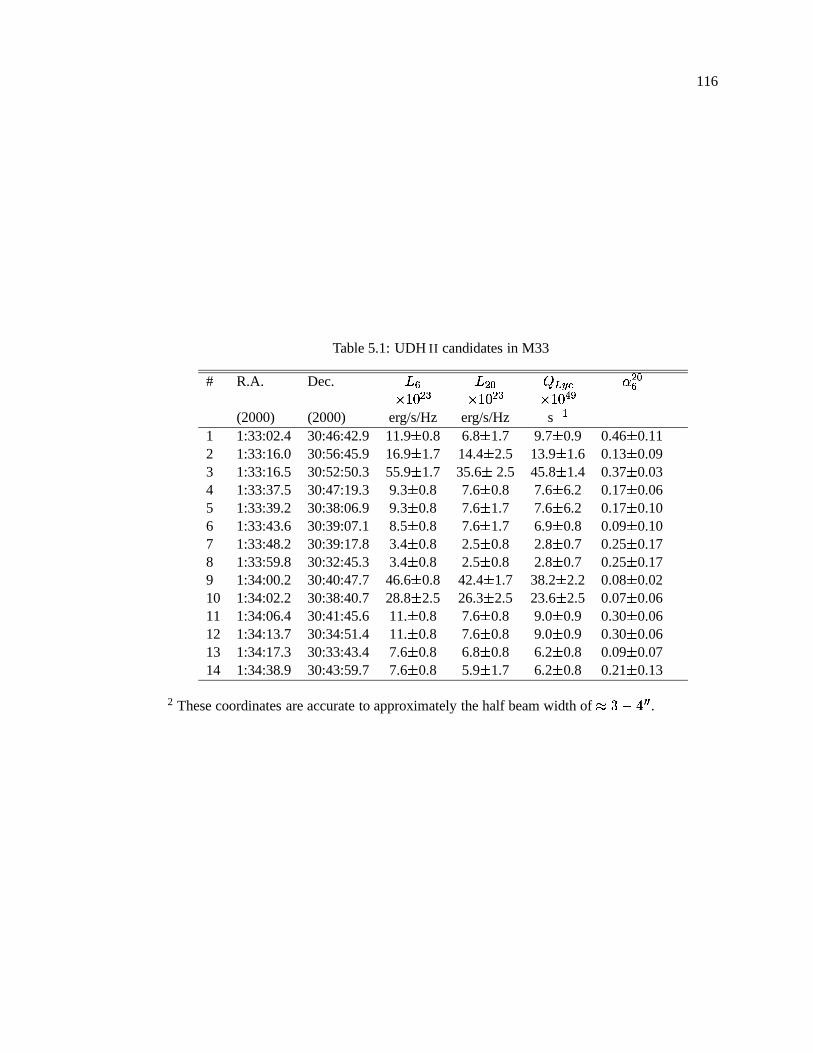
116
Table 5.1: UDH II candidates in M33
# R.A. Dec. � � � � ���� �
�� � ��� � � � � � � � � � � � � � �
(2000) (2000) erg/s/Hz erg/s/Hz s ���1 1:33:02.4 30:46:42.9 11.9
�0.8 6.8
�1.7 9.7
�0.9 0.46
�0.11
2 1:33:16.0 30:56:45.9 16.9�
1.7 14.4�
2.5 13.9�
1.6 0.13�
0.093 1:33:16.5 30:52:50.3 55.9
�1.7 35.6
�2.5 45.8
�1.4 0.37
�0.03
4 1:33:37.5 30:47:19.3 9.3�
0.8 7.6�
0.8 7.6�
6.2 0.17�
0.065 1:33:39.2 30:38:06.9 9.3
�0.8 7.6
�1.7 7.6
�6.2 0.17
�0.10
6 1:33:43.6 30:39:07.1 8.5�
0.8 7.6�
1.7 6.9�
0.8 0.09�
0.107 1:33:48.2 30:39:17.8 3.4
�0.8 2.5
�0.8 2.8
�0.7 0.25
�0.17
8 1:33:59.8 30:32:45.3 3.4�
0.8 2.5�
0.8 2.8�
0.7 0.25�
0.179 1:34:00.2 30:40:47.7 46.6
�0.8 42.4
�1.7 38.2
�2.2 0.08
�0.02
10 1:34:02.2 30:38:40.7 28.8�
2.5 26.3�
2.5 23.6�
2.5 0.07�
0.0611 1:34:06.4 30:41:45.6 11.
�0.8 7.6
�0.8 9.0
�0.9 0.30
�0.06
12 1:34:13.7 30:34:51.4 11.�
0.8 7.6�
0.8 9.0�
0.9 0.30�
0.0613 1:34:17.3 30:33:43.4 7.6
�0.8 6.8
�0.8 6.2
�0.8 0.09
�0.07
14 1:34:38.9 30:43:59.7 7.6�
0.8 5.9�
1.7 6.2�
0.8 0.21�
0.13
2 These coordinates are accurate to approximately the half beam width of � � � � � � .
117
5.3 Results
5.3.1 Detection of UDH II Candidates
Our primary tool for distinguishing UDH IIs from other types of radio sources, such as
supernovae remnants (SNR), is the radio spectral index � (where�
� � � � ). While optically
thin sources have � � � � � � , optically thick sources have � � � � � � ( � approaches 2 in the
black body limit), and typical non-thermal objects have � � � � � � . Unfortunately, not all SNRs
obey this convention — as discussed in Chapter 4, there is a class of “plerionic” SNRs known to
have atypically flat spectral indices ( � � � � � � � � � � ). A second set of observations taken with
adequate time separation, such as those employed in Chapter 4, would by useful determining
possible variations in flux, which might be attributable to SNe.
Consequently, in order to select UDH II candidates from the radio data, I have applied
the condition that these sources must have radio spectral indices � � � (higher fluxes at shorter
wavelengths). This criterion should exclude most other classes of radio-emitting objects, but
it may also exclude genuine UDH II regions depending upon the exact instrumental angular
resolution and frequencies observed. For example, low-frequency observations of optically
thick thermal sources could be contaminated by steep-spectrum non-thermal sources, such as
SNRs, and thus fail the � � � test, especially at longer wavelengths. Furthermore, more distant
sources, or sources observed using beam sizes larger than the thermal emitting region, may be
contaminated by steep-spectrum, non-thermal background emission that dominates the disks
and halos of most galaxies. Both of these effects will act to disguise an optically thick thermal
bremsstrahlung signature. Thermal sources with the lowest emission measure, and thus the
lowest free-free optical depth will be disguised the most strongly. Sources with the highest
emission measures are more likely to maintain a positive spectral signature and be correctly
identified. Fortunately, it is precisely these sources with high emission measures that are most
likely to host ultra-young stellar clusters.1 Distances as high as 10.1 Mpc have been estimated (e.g., Sandage & Tammann 1981).
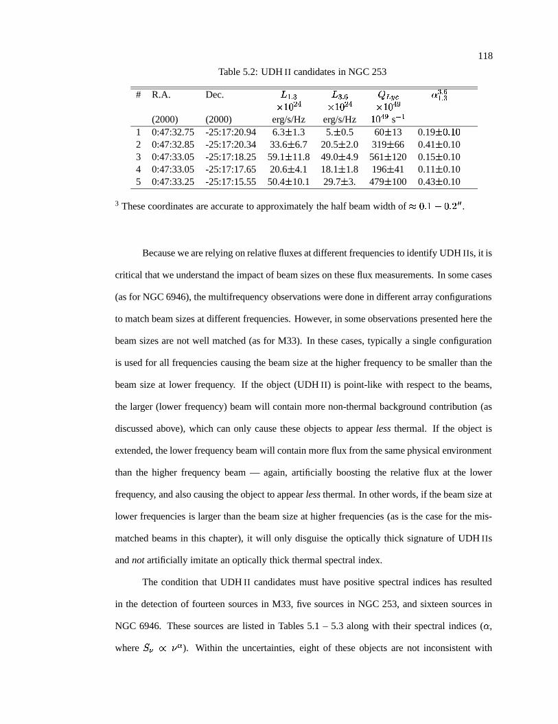
118
Table 5.2: UDH II candidates in NGC 253
# R.A. Dec. � � � � � ���� �
�� � �� �� � � � � � � � � � � � � � �
(2000) (2000) erg/s/Hz erg/s/Hz � � � �
s ���1 0:47:32.75 -25:17:20.94 6.3
�1.3 5.
�0.5 60
�13 0.19
� � � � �2 0:47:32.85 -25:17:20.34 33.6
�6.7 20.5
�2.0 319
�66 0.41
�0.10
3 0:47:33.05 -25:17:18.25 59.1�
11.8 49.0�
4.9 561�
120 0.15�
0.104 0:47:33.05 -25:17:17.65 20.6
�4.1 18.1
�1.8 196
�41 0.11
�0.10
5 0:47:33.25 -25:17:15.55 50.4�
10.1 29.7�
3. 479�
100 0.43�
0.10
3 These coordinates are accurate to approximately the half beam width of � � � � � � � � � � .
Because we are relying on relative fluxes at different frequencies to identify UDH IIs, it is
critical that we understand the impact of beam sizes on these flux measurements. In some cases
(as for NGC 6946), the multifrequency observations were done in different array configurations
to match beam sizes at different frequencies. However, in some observations presented here the
beam sizes are not well matched (as for M33). In these cases, typically a single configuration
is used for all frequencies causing the beam size at the higher frequency to be smaller than the
beam size at lower frequency. If the object (UDH II) is point-like with respect to the beams,
the larger (lower frequency) beam will contain more non-thermal background contribution (as
discussed above), which can only cause these objects to appear less thermal. If the object is
extended, the lower frequency beam will contain more flux from the same physical environment
than the higher frequency beam — again, artificially boosting the relative flux at the lower
frequency, and also causing the object to appear less thermal. In other words, if the beam size at
lower frequencies is larger than the beam size at higher frequencies (as is the case for the mis-
matched beams in this chapter), it will only disguise the optically thick signature of UDH IIs
and not artificially imitate an optically thick thermal spectral index.
The condition that UDH II candidates must have positive spectral indices has resulted
in the detection of fourteen sources in M33, five sources in NGC 253, and sixteen sources in
NGC 6946. These sources are listed in Tables 5.1 – 5.3 along with their spectral indices ( � ,
where�
� � � � ). Within the uncertainties, eight of these objects are not inconsistent with
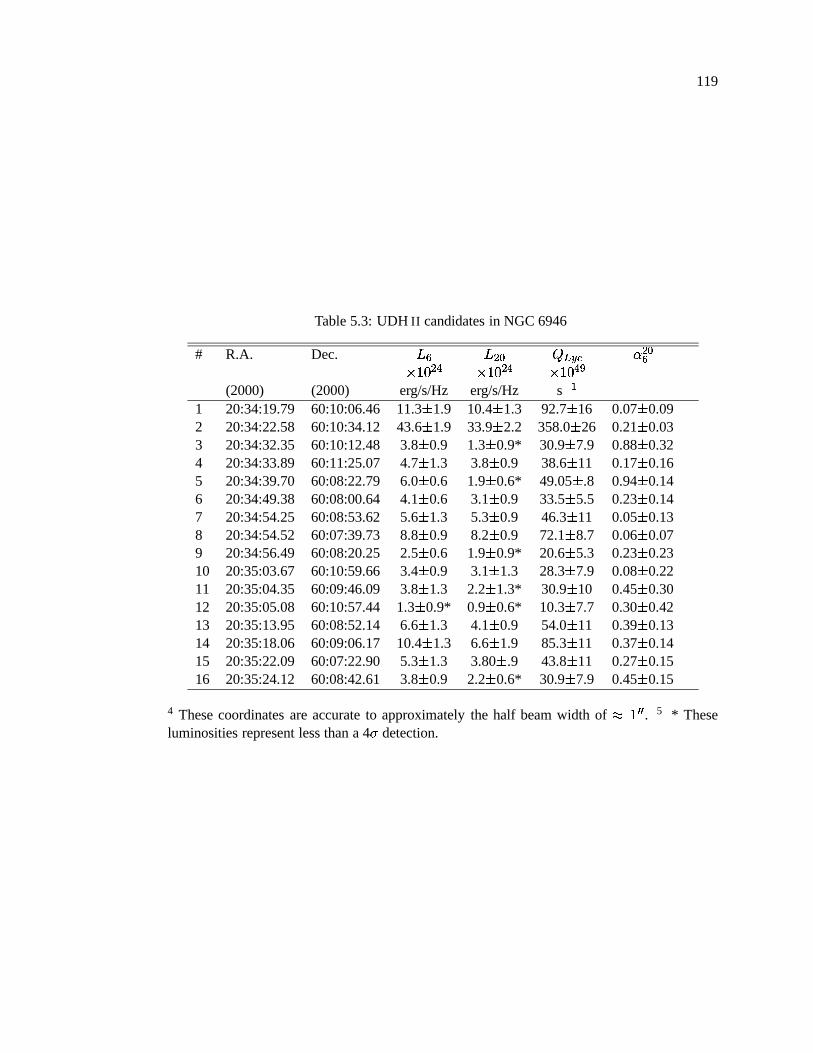
119
Table 5.3: UDH II candidates in NGC 6946
# R.A. Dec. � � � � ���� �
�� � ��� � � � � � � � � � � � � � �
(2000) (2000) erg/s/Hz erg/s/Hz s � �1 20:34:19.79 60:10:06.46 11.3
�1.9 10.4
�1.3 92.7
�16 0.07
�0.09
2 20:34:22.58 60:10:34.12 43.6�
1.9 33.9�
2.2 358.0�
26 0.21�
0.033 20:34:32.35 60:10:12.48 3.8
�0.9 1.3
�0.9* 30.9
�7.9 0.88
�0.32
4 20:34:33.89 60:11:25.07 4.7�
1.3 3.8�
0.9 38.6�
11 0.17�
0.165 20:34:39.70 60:08:22.79 6.0
�0.6 1.9
�0.6* 49.05
�.8 0.94
�0.14
6 20:34:49.38 60:08:00.64 4.1�
0.6 3.1�
0.9 33.5�
5.5 0.23�
0.147 20:34:54.25 60:08:53.62 5.6
�1.3 5.3
�0.9 46.3
�11 0.05
�0.13
8 20:34:54.52 60:07:39.73 8.8�
0.9 8.2�
0.9 72.1�
8.7 0.06�
0.079 20:34:56.49 60:08:20.25 2.5
�0.6 1.9
�0.9* 20.6
�5.3 0.23
�0.23
10 20:35:03.67 60:10:59.66 3.4�
0.9 3.1�
1.3 28.3�
7.9 0.08�
0.2211 20:35:04.35 60:09:46.09 3.8
�1.3 2.2
�1.3* 30.9
�10 0.45
�0.30
12 20:35:05.08 60:10:57.44 1.3�
0.9* 0.9�
0.6* 10.3�
7.7 0.30�
0.4213 20:35:13.95 60:08:52.14 6.6
�1.3 4.1
�0.9 54.0
�11 0.39
�0.13
14 20:35:18.06 60:09:06.17 10.4�
1.3 6.6�
1.9 85.3�
11 0.37�
0.1415 20:35:22.09 60:07:22.90 5.3
�1.3 3.80
�.9 43.8
�11 0.27
�0.15
16 20:35:24.12 60:08:42.61 3.8�
0.9 2.2�
0.6* 30.9�
7.9 0.45�
0.15
4 These coordinates are accurate to approximately the half beam width of � � � � . 5 * Theseluminosities represent less than a 4 � detection.
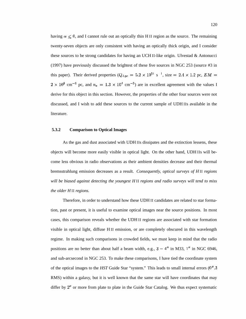
120
having � � ��� , and I cannot rule out an optically thin H II region as the source. The remaining
twenty-seven objects are only consistent with having an optically thick origin, and I consider
these sources to be strong candidates for having an UCH II-like origin. Ulvestad & Antonucci
(1997) have previously discussed the brightest of these five sources in NGC 253 (source #3 in
this paper). Their derived properties (��� �
�� � � � � � � � � s ��� , size � � � � � � � � pc,
� � �
� � � � �
cm �� pc, and ��� � � � � � � � � cm � � ) are in excellent agreement with the values I
derive for this object in this section. However, the properties of the other four sources were not
discussed, and I wish to add these sources to the current sample of UDH IIs available in the
literature.
5.3.2 Comparison to Optical Images
As the gas and dust associated with UDH IIs dissipates and the extinction lessens, these
objects will become more easily visible in optical light. On the other hand, UDH IIs will be-
come less obvious in radio observations as their ambient densities decrease and their thermal
bremsstrahlung emission decreases as a result. Consequently, optical surveys of H II regions
will be biased against detecting the youngest H II regions and radio surveys will tend to miss
the older H II regions.
Therefore, in order to understand how these UDH II candidates are related to star forma-
tion, past or present, it is useful to examine optical images near the source positions. In most
cases, this comparison reveals whether the UDH II regions are associated with star formation
visible in optical light, diffuse H II emission, or are completely obscured in this wavelength
regime. In making such comparisons in crowded fields, we must keep in mind that the radio
positions are no better than about half a beam width, e.g.,� � � � � in M33, � � � in NGC 6946,
and sub-arcsecond in NGC 253. To make these comparisons, I have tied the coordinate system
of the optical images to the HST Guide Star “system.” This leads to small internal errors ( � � � � �
RMS) within a galaxy, but it is well known that the same star will have coordinates that may
differ by � � � or more from plate to plate in the Guide Star Catalog. We thus expect systematic
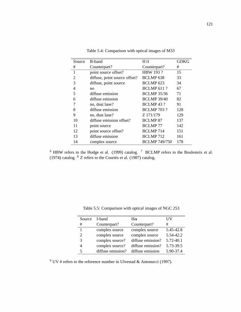
121
Table 5.4: Comparison with optical images of M33
Source B-band H II GDKG# Counterpart? Counterpart? #1 point source offset? HBW 193 ? 152 diffuse, point source offset? BCLMP 638 333 diffuse, point source BCLMP 623 344 no BCLMP 611 ? 675 diffuse emission BCLMP 35/36 716 diffuse emission BCLMP 39/40 827 no, dust lane? BCLMP 43 ? 918 diffuse emission BCLMP 703 ? 1289 no, dust lane? Z 171/179 12910 diffuse emission offset? BCLMP 87 13711 point source BCLMP 77 14212 point source offset? BCLMP 714 15113 diffuse emission BCLMP 712 16114 complex source BCLMP 749/750 178
6 HBW refers to the Hodge et al. (1999) catalog. 7 BCLMP refers to the Boulesteix et al.(1974) catalog. 8 Z refers to the Courtes et al. (1987) catalog.
Table 5.5: Comparison with optical images of NGC 253
Source I-band H � UV# Counterpart? Counterpart? #1 complex source complex source 5.45-42.82 complex source complex source 5.54-42.23 complex source? diffuse emission? 5.72-40.14 complex source? diffuse emission? 5.73-39.55 diffuse emission? diffuse emission 5.90-37.4
9 UV # refers to the reference number in Ulvestad & Antonucci (1997).
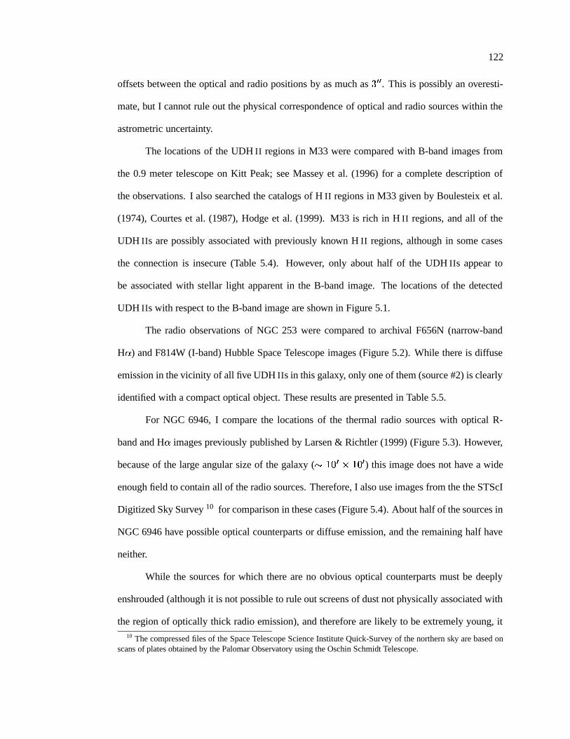
122
offsets between the optical and radio positions by as much as� � �
. This is possibly an overesti-
mate, but I cannot rule out the physical correspondence of optical and radio sources within the
astrometric uncertainty.
The locations of the UDH II regions in M33 were compared with B-band images from
the 0.9 meter telescope on Kitt Peak; see Massey et al. (1996) for a complete description of
the observations. I also searched the catalogs of H II regions in M33 given by Boulesteix et al.
(1974), Courtes et al. (1987), Hodge et al. (1999). M33 is rich in H II regions, and all of the
UDH IIs are possibly associated with previously known H II regions, although in some cases
the connection is insecure (Table 5.4). However, only about half of the UDH IIs appear to
be associated with stellar light apparent in the B-band image. The locations of the detected
UDH IIs with respect to the B-band image are shown in Figure 5.1.
The radio observations of NGC 253 were compared to archival F656N (narrow-band
H � ) and F814W (I-band) Hubble Space Telescope images (Figure 5.2). While there is diffuse
emission in the vicinity of all five UDH IIs in this galaxy, only one of them (source #2) is clearly
identified with a compact optical object. These results are presented in Table 5.5.
For NGC 6946, I compare the locations of the thermal radio sources with optical R-
band and H � images previously published by Larsen & Richtler (1999) (Figure 5.3). However,
because of the large angular size of the galaxy ( � � � � � � � � ) this image does not have a wide
enough field to contain all of the radio sources. Therefore, I also use images from the the STScI
Digitized Sky Survey 10 for comparison in these cases (Figure 5.4). About half of the sources in
NGC 6946 have possible optical counterparts or diffuse emission, and the remaining half have
neither.
While the sources for which there are no obvious optical counterparts must be deeply
enshrouded (although it is not possible to rule out screens of dust not physically associated with
the region of optically thick radio emission), and therefore are likely to be extremely young, it10 The compressed files of the Space Telescope Science Institute Quick-Survey of the northern sky are based on
scans of plates obtained by the Palomar Observatory using the Oschin Schmidt Telescope.
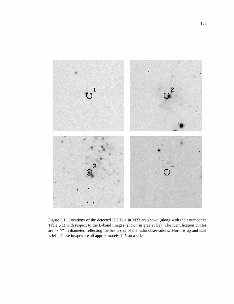
123
Figure 5.1: Locations of the detected UDH IIs in M33 are shown (along with their number inTable 5.1) with respect to the B-band images (shown in gray scale). The identification circlesare � � � �
in diameter, reflecting the beam size of the radio observations. North is up and Eastis left. These images are all approximately � � � � on a side.
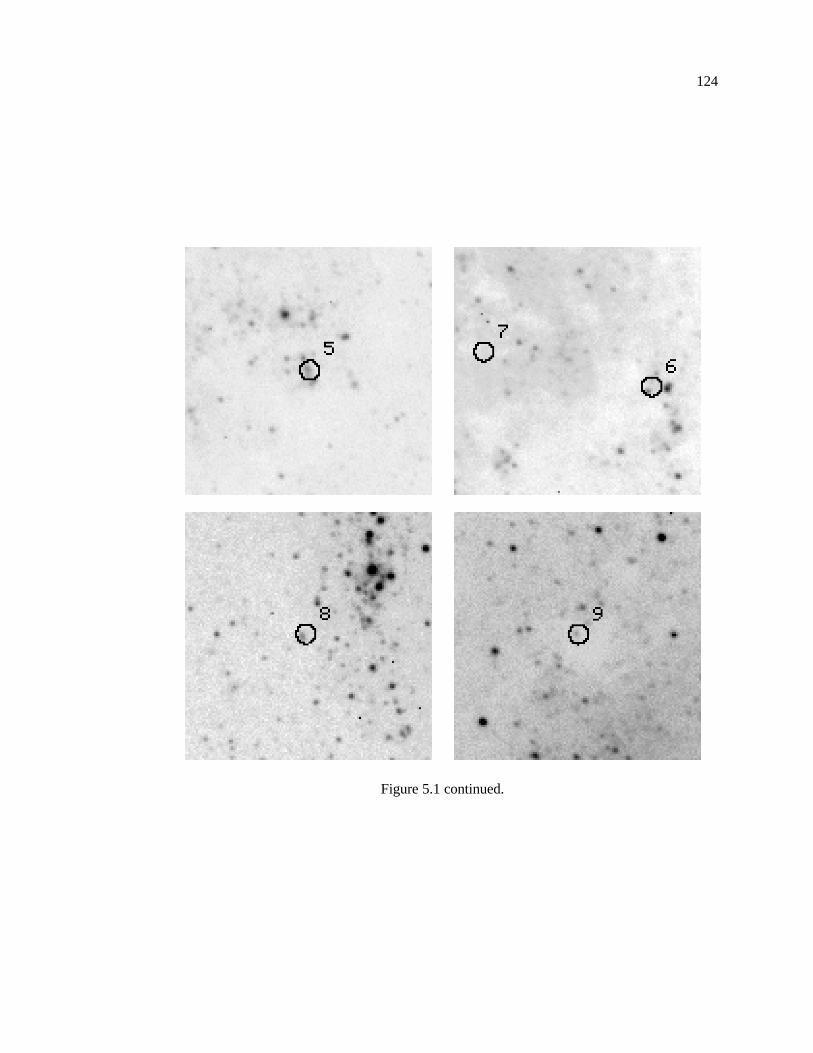
124
Figure 5.1 continued.
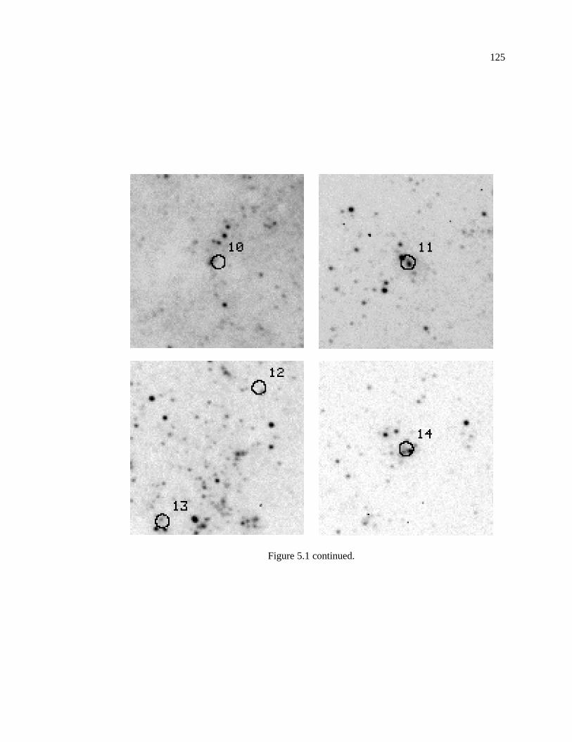
125
Figure 5.1 continued.
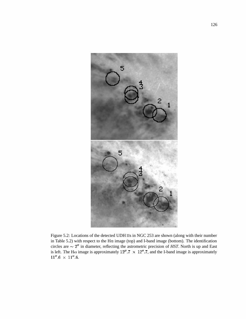
126
Figure 5.2: Locations of the detected UDH IIs in NGC 253 are shown (along with their numberin Table 5.2) with respect to the H � image (top) and I-band image (bottom). The identificationcircles are � � � � in diameter, reflecting the astrometric precision of HST. North is up and Eastis left. The H � image is approximately � � � � � � � � � � � � � , and the I-band image is approximately� � � � � � � � � � � � � .
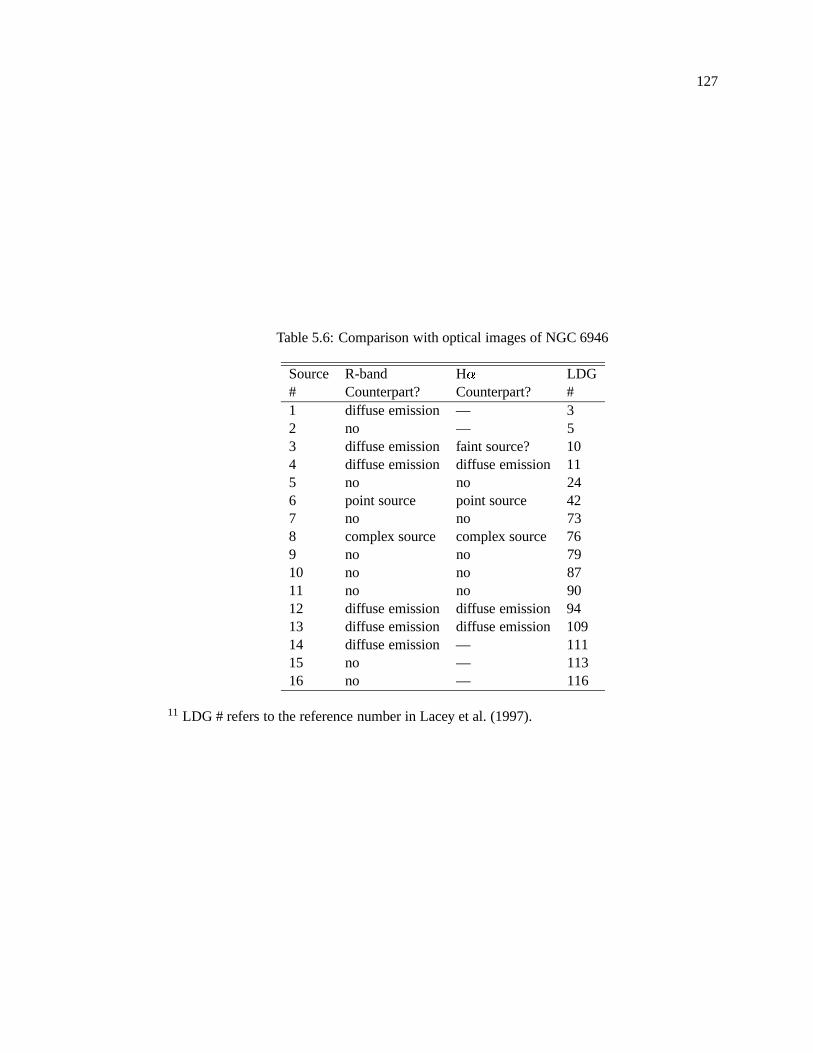
127
Table 5.6: Comparison with optical images of NGC 6946
Source R-band H � LDG# Counterpart? Counterpart? #1 diffuse emission — 32 no — 53 diffuse emission faint source? 104 diffuse emission diffuse emission 115 no no 246 point source point source 427 no no 738 complex source complex source 769 no no 7910 no no 8711 no no 9012 diffuse emission diffuse emission 9413 diffuse emission diffuse emission 10914 diffuse emission — 11115 no — 11316 no — 116
11 LDG # refers to the reference number in Lacey et al. (1997).
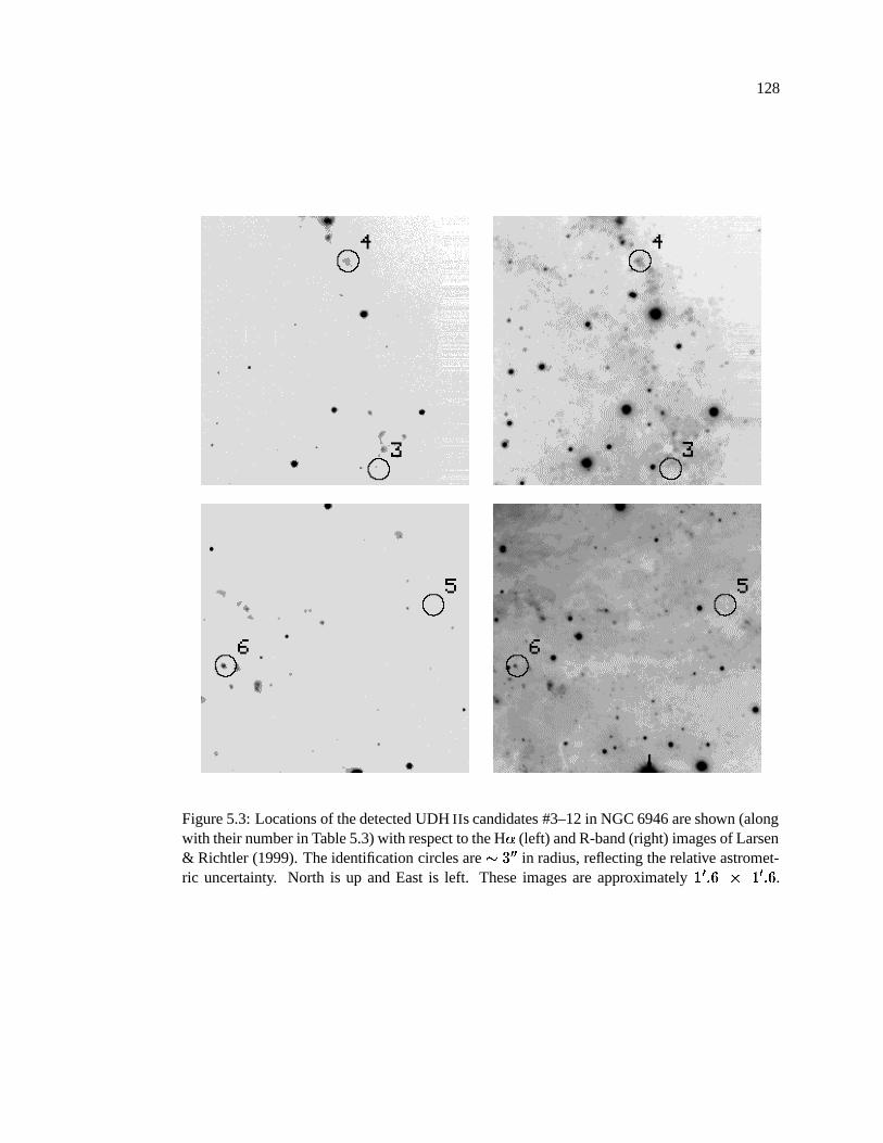
128
Figure 5.3: Locations of the detected UDH IIs candidates #3–12 in NGC 6946 are shown (alongwith their number in Table 5.3) with respect to the H � (left) and R-band (right) images of Larsen& Richtler (1999). The identification circles are � � � � in radius, reflecting the relative astromet-ric uncertainty. North is up and East is left. These images are approximately � � � � � � � � � .
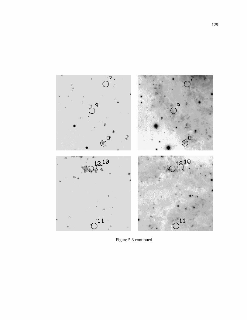
129
Figure 5.3 continued.
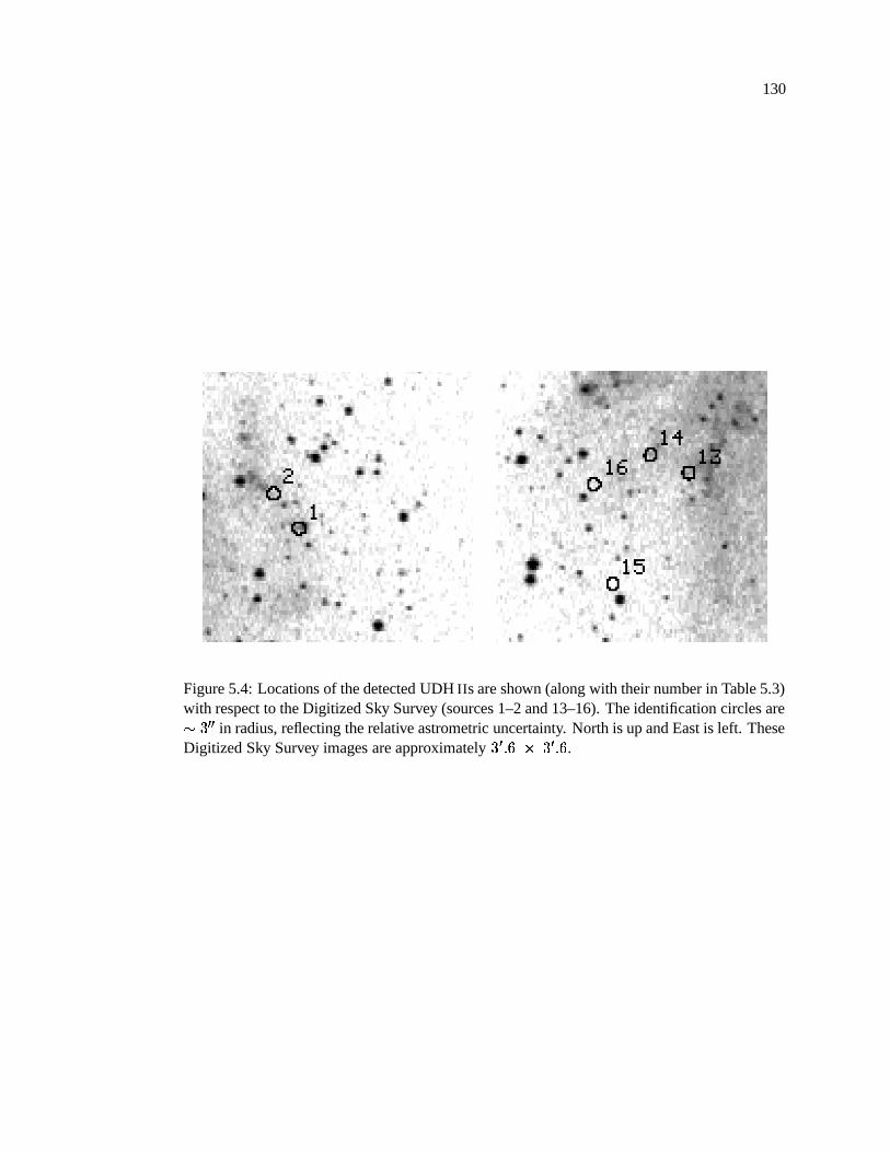
130
Figure 5.4: Locations of the detected UDH IIs are shown (along with their number in Table 5.3)with respect to the Digitized Sky Survey (sources 1–2 and 13–16). The identification circles are� � � � in radius, reflecting the relative astrometric uncertainty. North is up and East is left. TheseDigitized Sky Survey images are approximately
� �� � ��� �
� � .
131
is not clear whether detection of light in the optical regime rules out extreme youth for UDH II
regions. I make this tentative statement for several reasons: (1) in most cases presented in this
sample, the identification of an optical counterpart is insecure due to the possible systematics
between the optical and radio positions, as well as the relatively large synthesized radio beam-
width for M33; (2) in cases where individual stars are resolved (M33), the number of stars
required to create the Lyman continuum flux are not apparent in the optical images, suggesting
either a misidentification due to pointing uncertainty, or a number of the individual stars are, in
fact, still enshrouded. This scenario has actually been observed in the galactic UCH II complex
W49A where some of the stars in the complex appear to have emerged from their birth cocoons
while the rest of the complex remains enshrouded (Conti & Blum 2001) ; and (3) if the dominant
source of opacity is Thomson scattering (and not dust), a source with a radius of 5 pc could have
electron densities as high as � � � � � � cm � � and still have opacities as low as � � � (although
it is difficult to imagine how newly formed stars could be in an environment absent of dust).
Therefore, I conclude that the possible identification of optical counterparts does not
preclude the youth of these objects. However, the sources for which there are no optical coun-
terparts are more likely deeply embedded in their natal molecular clouds, and therefore are more
likely to be extremely young.
5.3.3 Modeled Properties
Given the luminosities and radio spectral energy distributions of H II regions, their phys-
ical parameters such as size and electron density can be estimated. Again using the analytical
approximation of Mezger & Henderson (1967) (as in Chapter 4), I can estimate the emission
measure,� � � � � �� � � , given an electron temperature, � , the observing frequency, � , and the
optical depth at that frequency.
� � � � � � � ��� � � � � � ��� ���� � � � � � � �
� ����� � � � � � � (5.1)
The positive spectral index for these sources arises from free-free emission where � � ��� ,
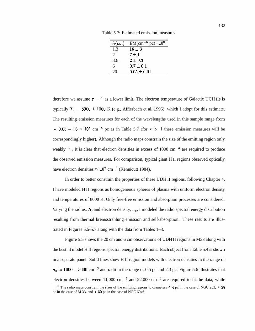
132
Table 5.7: Estimated emission measures
� � � � � EM(cm � � pc)� � � �
1.3 � � � �
2� � �
3.6 � � � � �6 � � � � � � �20 � � � � � � � � �
therefore we assume � � � as a lower limit. The electron temperature of Galactic UCH IIs is
typically ��� � � � � � � � � � � K (e.g., Afflerbach et al. 1996), which I adopt for this estimate.
The resulting emission measures for each of the wavelengths used in this sample range from
� � � � � � � � � � � �
cm �� pc as in Table 5.7 (for � � � these emission measures will be
correspondingly higher). Although the radio maps constrain the size of the emitting region only
weakly 12 , it is clear that electron densities in excess of 1000 cm � � are required to produce
the observed emission measures. For comparison, typical giant H II regions observed optically
have electron densities � � � � cm � � (Kennicutt 1984).
In order to better constrain the properties of these UDH II regions, following Chapter 4,
I have modeled H II regions as homogeneous spheres of plasma with uniform electron density
and temperatures of 8000 K. Only free-free emission and absorption processes are considered.
Varying the radius, , and electron density, � � , I modeled the radio spectral energy distribution
resulting from thermal bremsstrahlung emission and self-absorption. These results are illus-
trated in Figures 5.5-5.7 along with the data from Tables 1–3.
Figure 5.5 shows the 20 cm and 6 cm observations of UDH II regions in M33 along with
the best fit model H II regions spectral energy distributions. Each object from Table 5.4 is shown
in a separate panel. Solid lines show H II region models with electron densities in the range of
��� � � � � � � � � � � cm �� and radii in the range of 0.5 pc and 2.3 pc. Figure 5.6 illustrates that
electron densities between 11,000 cm � � and 22,000 cm � � are required to fit the data, while12 The radio maps constrain the sizes of the emitting regions to diameters
� � pc in the case of NGC 253,� � �
pc in the case of M 33, and ��� � pc in the case of NGC 6946
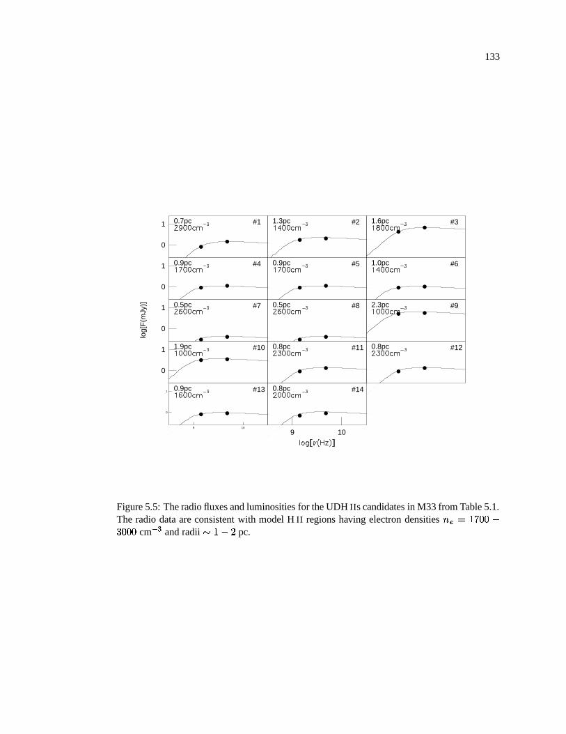
133
0
1 #10.7pc #21.3pc #31.6pc
0
1 #40.9pc #50.9pc #61.0pc
0
1 #70.5pc
log[
F(m
Jy)] #80.5pc #92.3pc
0
1 #101.9pc #110.8pc #120.8pc
9 10
0
1 #130.9pc
9 10
#140.8pc
Figure 5.5: The radio fluxes and luminosities for the UDH IIs candidates in M33 from Table 5.1.The radio data are consistent with model H II regions having electron densities ��� � � � � � �� � � � cm � � and radii � � � � pc.
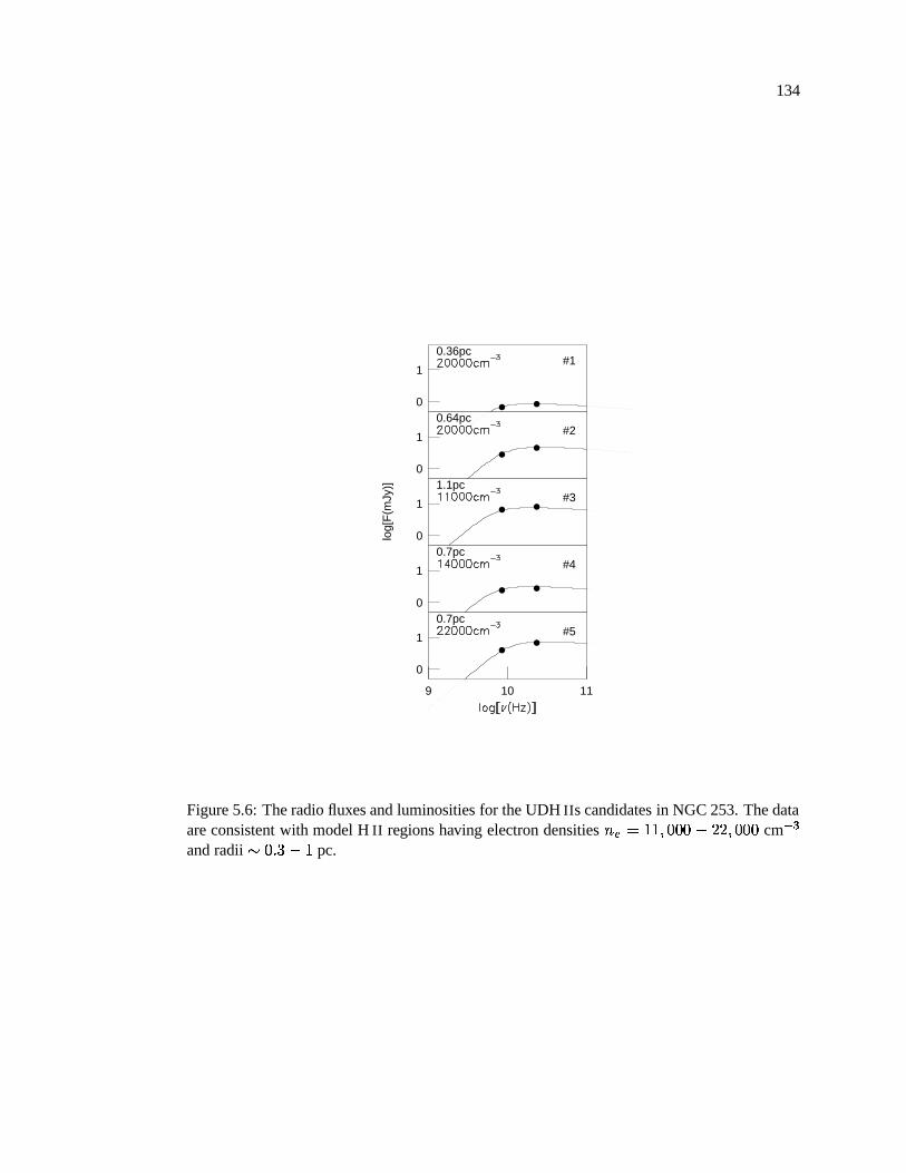
134
0
1#1
0.36pc
0
1 #20.64pc
0
1 #31.1pc
log[
F(m
Jy)]
0
1 #40.7pc
9 10 11
0
1 #50.7pc
Figure 5.6: The radio fluxes and luminosities for the UDH IIs candidates in NGC 253. The dataare consistent with model H II regions having electron densities � � � � � � � � � � � � � � � � cm � �and radii � � � � � � pc.
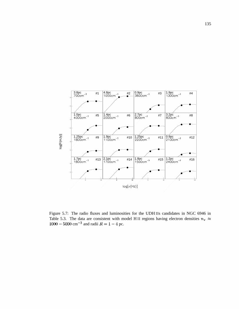
135
-1
0
#13.8pc #24.8pc #30.9pc #41.9pc
-1
0
#51.0pc #61.4pc #72.7pc #83.2pc
-1
0
#91.25pc
lo
g[F
(mJy
)]
#101.9pc #111.25pc #120.9pc
9 10
-1
0
#131.7pc
9 109 10
#142.1pc
9 10
#151.8pc
9 10
#161.2pc
Figure 5.7: The radio fluxes and luminosities for the UDH IIs candidates in NGC 6946 inTable 5.3. The data are consistent with model H II regions having electron densities ��� �� � � � � � � � � cm � � and radii � � � � pc.
136
the best fit radii are all � � � pc. Not only are the UDH II regions in NGC 253 intrinsically
more luminous than in the other two galaxies, they also have higher densities. In the case of
NGC 253, observations reveal that the UDH II regions are optically thick at frequencies as high
as 15 GHz. In the case of NGC 6946, densities of 700 cm � � to 4000 cm �� fit the 20 cm and
6 cm data for radii ranging from � 1 pc to 5 pc.
It is reasonable to ask whether the simple homogeneous sphere models presented here
are sufficient to infer the physical characteristics (sizes, densities) of the UDH IIs. Realistically,
we expect that the radio sources identified as UDH IIs are not simply monolithic dense H II
regions. Rather, we might expect that they are collections of several hundred ultra-compact
H II regions (� � � � � � cm � � � � � � � pc) embedded in a more tenuous inter-UCH II medium
(see � 5.4.2). However, NGC 5253 (Turner et al. 2000) is near enough and have observations
with high enough resolution that the radio imaging can directly constrain the sizes of the emit-
ting regions without recourse to model assumptions. In this case, the simple homogeneous
spherical models described above produce size estimates in excellent agreement with the high-
resolution radio maps. The deconvolved diameters of the radio the single UDH II radio source
in NGC 5253 has a deconvolved diameter of � � pc (Turner et al. 2000), consistent with the
expectations of the simple model predictions based on their observed radio luminosities. As
further support for our simple models, recently Mohan et al. (2001) have made slightly more
sophisticated multi-density models for radio recombination line observations of He 2-10 and
and NGC 5253; their results are in excellent agreement with the results obtained with these
simple models.
Given the agreement in this cases, I believe that the simple two-parameter models are
sufficiently instructive to make meaningful inferences about the sizes and densities of UDH IIs
based on radio continuum luminosities. More realistic models would include an arbitrary num-
ber of UCH II regions within each UDH II each with its own density profile, and an inter-
UCH II medium with a specified density profile and temperature distribution. However, relaxing
the simple two-parameter approach results in the number of free parameters and computational
137
complexity growing rapidly.
5.4 Discussion
5.4.1 Stellar Content
The production rate of Lyman continuum photons, and, thus, the stellar content of each
UDH II region can be estimated from the thermal radio luminosity following Condon (1992) as
in Chapter 4,
��� ��� � � � � � � � � � ��� � ���
� � � � � � � � � �
������� � � � � � � � � � � �
� � � � � � � � ��� ��� � � � � (5.2)
Since the non-thermal component becomes weaker at higher frequencies, for each of the UDH IIs
in this sample we use the luminosity measured at the highest frequency in each data set to deter-
mine��� �
� . The resulting values determined from this method are presented in Tables 5.1 – 5.3.
One should also bear in mind that the��� �
� values determined with this method could suffer
from two different problems: (1) if the source is, in fact, optically thick even at the highest
frequencies measured, this method will underestimate the actual ionizing luminosity, and (2)
if there is contamination from background non-thermal emission in the beam at the frequency
used, the ionizing luminosity will be overestimated. While these two issues have an opposite
effect on��� �
� , we might expect the impact of (2) to be negligible as discussed in Chapter 4.
The production rate of Lyman continuum photons from these sources can be used to
estimate the number of massive stars powering the observed emission. Following the convention
of Vacca (1994), a “typical” O-star (type O7V) produces� � �
�� � � � � � � � �
s � � . Therefore,
the��� �
� values in Tables 5.1-5.3 can be directly translated into the number of “equivalent”
O7V stars (O7V*). Using this method, we see that the UDH II regions in this sample have
� � � � � O7V* stars in M33, � � � � � � � in NGC 253, and � � � � � � � in NGC 6946.
Moreover, the total stellar mass of these objects can be estimated using the Starburst99 models
of Leitherer et al. (1999) with solar metallicity, Salpeter IMF, and lower and upper mass cutoffs
of 1 M and 100 M , respectively (decreasing the lower mass limit will increase the total stellar
138
mass estimate). Using these parameters, star clusters producing this range of Lyman continuum
photons at ages � � � � Myr would have total masses of � � � � � � � � � � M .
These��� �
� and mass values are smaller than those found for the UDH IIs in He 2-10 and
in NGC 5253 (Turner et al. 2000), which have �� � � O7V* stars and masses ��� � � M . This is
not a surprising result — it is likely that we will only find massive star clusters forming in intense
starburst events; Elmegreen & Efremov (1997) have demonstrated the need for extremely high-
pressure environments, such as those found in starburst galaxies, to produce bound massive star
clusters. However, in less formidable environments, we should expect to find a continuous range
of UDH IIs — from single UCH IIs and UCH II complexes (such as those found in the Galaxy),
to the massive bound clusters (such as those found in NGC 5253, He 2-10, and NGC 2146) that
may evolve into globular clusters. The sample presented in this chapter is beginning to fill in
this continuum of objects for the first time.
5.4.2 Comparison to W49A
One of the most well studied UCH II complexes in the Galaxy is W49A, which makes it
well suited for comparison to the UDH II regions in this sample. First detected by Westerhout
(1958) in his radio survey, W49A has since been resolved into at least 30 UCH II regions (de
Pree et al. 1997), and is estimated to have � � � � O7V* stars (Smith et al. 1978; Vacca 1994).
It also appears that a few of the stars in W49A have begun to emerge from their birth cocoons
while the rest of the cluster remains deeply enshrouded (Conti & Blum 2001). W49A is � � �
pc in diameter (de Pree et al. 1997), and would fit within the beam sizes utilized in this chapter
if located at the same distances as the galaxies in this sample; W49A would have angular sizes
of � � � � � � , � � � � � , and � � � � � , respectively, in M33, NGC 253, and NGC 6946. Because W49A is
significantly closer (� � � � � � kpc; Gwinn et al. 1992), than the galaxies presented in this paper,
any observations I use for comparison need to be at sufficiently low resolution as to include the
entire W49A region. This condition is well-satisfied by the pioneering observations of Mezger
et al. (1967), who obtained � � � � � resolution radio maps of W49A at several wavelengths.
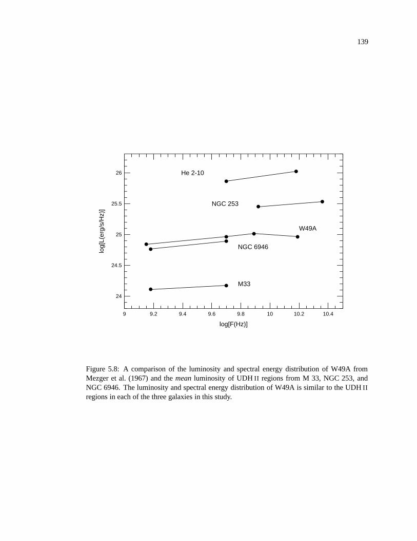
139
9 9.2 9.4 9.6 9.8 10 10.2 10.4
24
24.5
25
25.5
26 He 2-10
W49A
NGC 253
M33
NGC 6946
log[F(Hz)]
log[
L(er
g/s/
Hz)
]
Figure 5.8: A comparison of the luminosity and spectral energy distribution of W49A fromMezger et al. (1967) and the mean luminosity of UDH II regions from M 33, NGC 253, andNGC 6946. The luminosity and spectral energy distribution of W49A is similar to the UDH IIregions in each of the three galaxies in this study.
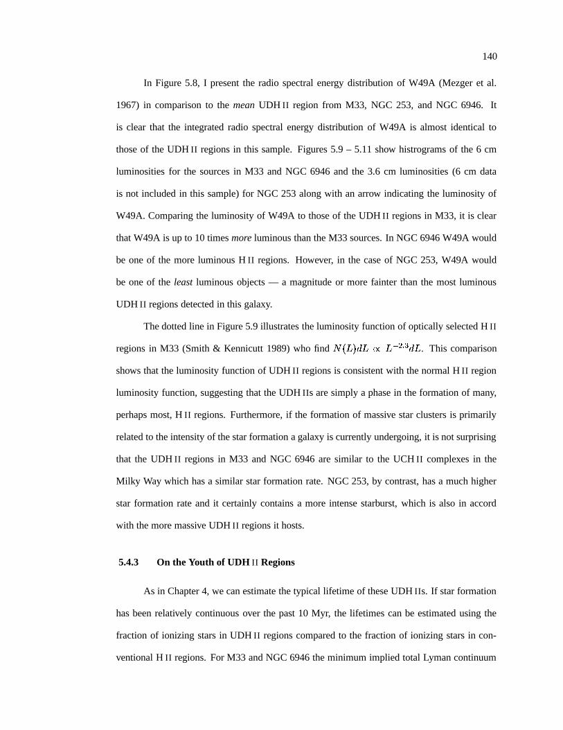
140
In Figure 5.8, I present the radio spectral energy distribution of W49A (Mezger et al.
1967) in comparison to the mean UDH II region from M33, NGC 253, and NGC 6946. It
is clear that the integrated radio spectral energy distribution of W49A is almost identical to
those of the UDH II regions in this sample. Figures 5.9 – 5.11 show histrograms of the 6 cm
luminosities for the sources in M33 and NGC 6946 and the 3.6 cm luminosities (6 cm data
is not included in this sample) for NGC 253 along with an arrow indicating the luminosity of
W49A. Comparing the luminosity of W49A to those of the UDH II regions in M33, it is clear
that W49A is up to 10 times more luminous than the M33 sources. In NGC 6946 W49A would
be one of the more luminous H II regions. However, in the case of NGC 253, W49A would
be one of the least luminous objects — a magnitude or more fainter than the most luminous
UDH II regions detected in this galaxy.
The dotted line in Figure 5.9 illustrates the luminosity function of optically selected H II
regions in M33 (Smith & Kennicutt 1989) who find� � ��� � � � � ��� � � � . This comparison
shows that the luminosity function of UDH II regions is consistent with the normal H II region
luminosity function, suggesting that the UDH IIs are simply a phase in the formation of many,
perhaps most, H II regions. Furthermore, if the formation of massive star clusters is primarily
related to the intensity of the star formation a galaxy is currently undergoing, it is not surprising
that the UDH II regions in M33 and NGC 6946 are similar to the UCH II complexes in the
Milky Way which has a similar star formation rate. NGC 253, by contrast, has a much higher
star formation rate and it certainly contains a more intense starburst, which is also in accord
with the more massive UDH II regions it hosts.
5.4.3 On the Youth of UDH II Regions
As in Chapter 4, we can estimate the typical lifetime of these UDH IIs. If star formation
has been relatively continuous over the past 10 Myr, the lifetimes can be estimated using the
fraction of ionizing stars in UDH II regions compared to the fraction of ionizing stars in con-
ventional H II regions. For M33 and NGC 6946 the minimum implied total Lyman continuum
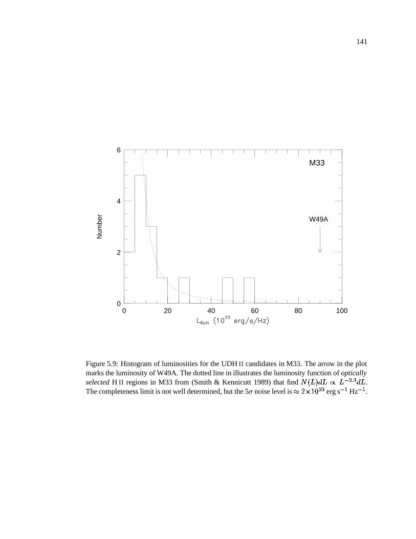
141
0 20 40 60 80 1000
2
4
6
Num
ber
W49A
M33
Figure 5.9: Histogram of luminosities for the UDH II candidates in M33. The arrow in the plotmarks the luminosity of W49A. The dotted line in illustrates the luminosity function of opticallyselected H II regions in M33 from (Smith & Kennicutt 1989) that find
� � ��� � � � � � � � � � .The completeness limit is not well determined, but the 5 � noise level is ��� � � � � � erg s ��� Hz ��� .
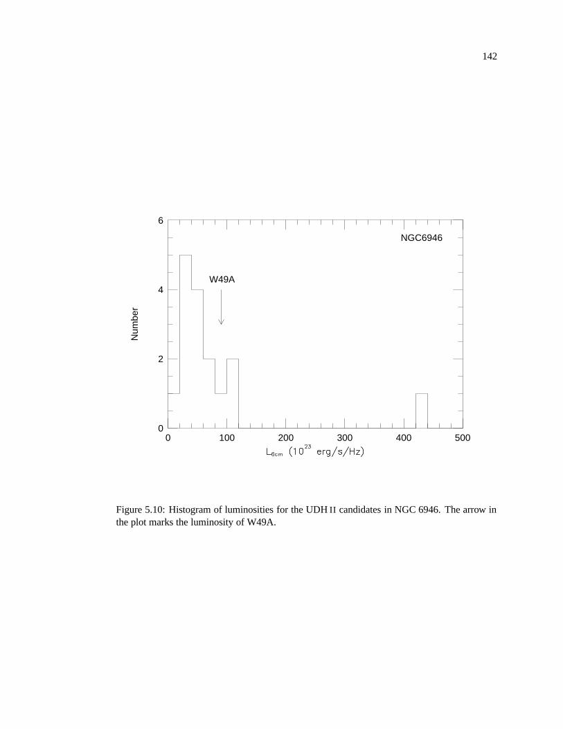
142
0 100 200 300 400 5000
2
4
6
Num
ber
W49A
NGC6946
Figure 5.10: Histogram of luminosities for the UDH II candidates in NGC 6946. The arrow inthe plot marks the luminosity of W49A.
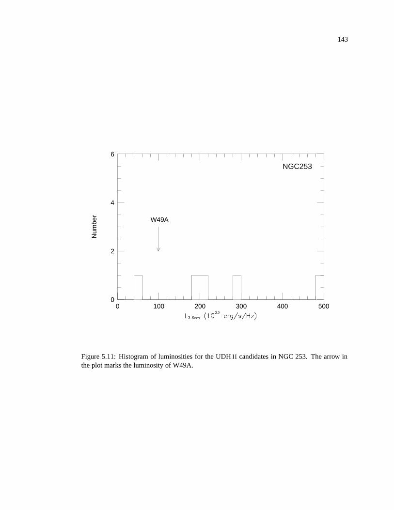
143
0 100 200 300 400 5000
2
4
6
Num
ber
W49A
NGC253
Figure 5.11: Histogram of luminosities for the UDH II candidates in NGC 253. The arrow inthe plot marks the luminosity of W49A.
144
photon production rate,��� �
� , of the UDH II regions is � � � � � � � � s ��� and � � � � � � � s � � re-
spectively (provided there is no leakage from the enshrouding cocoon that would likely result
in associated H � emission). The total��� �
� for the entire galaxy is� � � � � � s � � for M33 and
� � � � � � � � s � � for NGC 6946 (Kennicutt 1983 scaled to our adopted distance). Thus, the UDH II
regions contain 1% and 7% of the total ionizing photons. If the star formation has been rea-
sonably continuous in these systems, a plausible estimate for the typical duration of the UDH II
phase is 0.01 to 0.07 times the typical H II region lifetime ( � � � � yr). This implies a mean age
of less than 1 Myr for UDH II regions, in excellent agreement with the lifetimes estimated in
Chapter 4.
Chapter 6
Future Work
The discovery of UDH IIs has opened up a new field, allowing us to study the earlist
stages of massive star cluster evolution for the first time as well as the influence this mode of
star formation has had throughout the universe. As with any fledgling field, there is a great
deal of knowledge and understanding yet to be worked out, and many questions remain. Future
work will reveal the physical properties of these ultra-young massive star clusters and determine
the conditions required for their formation. In addition to studying their earliest developmental
stages, we will determine the properties of massive star clusters as they evolve and develop an
evolutionary sequence. This work will have a direct impact on our understanding of both stellar
and galactic evolution, as well as the origin of globular clusters and the physical conditions in
the early universe required to create these massive clusters so prodigiously.
6.1 Expand the Sample of Known UDH IIs
Because UDH IIs have only recently been discovered, one of the most fundamental goals
in this field is simply to expand the sample of known objects in order to better understand their
properties in a statistical sense. For example, once we have obtained a large enough sample
we will be able to construct an initial mass function for clusters and examine its dependence
on different physical environments. This result will be absolutely crucial in understanding the
physics of star formation via molecular cloud collapse.
High resolution radio telescopes, such as the Very Large Array (VLA), are ideally suited
146
for conducting surveys of starburst galaxies at high radio frequencies (such as 5 and 20 GHz)
in order to detect the characteristic optically-thick thermal spectral energy distribution of these
compact sources. Because radio wavelengths do not suffer from dust extinction, we will be
able to probe even the most dense and obscured star forming regions in starburst galaxies.
To this end, I have already begun observing campaigns with the VLA, the Multi-Element
Radio Linked Interferometer Network (MERLIN), and the Australia Telescope Compact Ar-
ray (ATCA) with observations already made of eight additional Wolf-Rayet galaxies (MRK 8,
MRK 33, NGC 3395, NGC 3396, IC 4662, NGC 5398, NGC 1705, and NGC 4449). In addi-
tion, I have begun a survey with ATCA (at 3 cm and 6 cm) of radio sources in the Magellanic
Clouds in order to extend our knowledge of individual UCH II regions beyond the Galaxy.
6.2 Determine the Properties of the Birth Environments of Massive Star Clus-
ters
One of my main objectives for the future is to determine the physical properties required
to form massive bound clusters. We know that in the local universe, massive star clusters appear
to be formed exclusively in starbursting regions of galaxies. However, we have never directly
probed the environmental conditions of their formation. Similar physical conditions must have
been present in the early universe in order to create the vast number of old globular clusters
we see today (although metallicity is almost certainly an issue here, and studying the lowest
metallicity systems available will be critical for this interpretation).
Because massive star clusters in their earliest stages are embedded in their natal molecu-
lar clouds, millimeter observations of molecular lines are particularly well suited for observing
their birth environments. The highly abundant CO lines can be used to trace the molecular gas
associated with UDH IIs, while higher dipole molecules, such as CS or HCN will map out the
highest density gas which is expected to be directly correlated with areas of star formation. We
can use molecular line diagnostics to provide information on all of the basic physical properties
of the natal environments, including their temperatures, densities, and pressures.

147
I have already obtained two tracks with the OVRO millimeter array (with the equatorial
and ultra-high resolution configurations; a track in the high configuration has not yet been ob-
served although the time was granted) to create a high spatial resolution map of the CO(1-0) line
in He 2-10, where we discovered five UDH IIs (see Chapter 4). I will also apply for time in the
coming semester using the BIMA millimeter array for a project mapping the physical properties
of the dense gas in the starburst galaxies known to host UDH IIs. In the more distant future, the
proposed (and not quite funded to date) Atacama Large Millimeter Array (ALMA, to be built
in the Atacama desert in Chile) will enable superb sub-arcsecond observations (similar to the
resolution of HST) to be obtained in the millimeter regime for the first time. This instrument
will be ideal for studying the physical properties of UDH IIs.
Another issue I wish to address is the relation between the morphology of warm/hot dust
and the UDH IIs. UDH IIs should be embedded in knots of bright and hot dust emission. To
date, only minimal mid-infrared data (such as that presented in Chapter 4) exists on UDH IIs,
but this dust has not yet been observed in detail. I plan to carry out a mid-infrared imaging and
spectroscopy campaign to directly measure the warm and hot dust associated with UDH IIs,
allowing us to establish the nature of this relationship.
6.3 Determine the Properties of Massive Star Clusters at Different Evolution-
ary Stages
As massive star clusters age and begin to emerge from their birth material, their phys-
ical properties will evolve rapidly. For example, in the earliest stages of their evolution, their
environment will transform from being optically thick to optically thin at radio wavelengths.
As the most massive stars begin to evolve, they will dramatically affect the cluster environment
via stellar winds and supernovae. After the ambient gas has been dissipated from the cluster,
much of the gravitational binding energy is lost and the clusters themselves may begin to dis-
sociate. Throughout these phases, the overall spectral energy distribution of these clusters will
also metamorphose. However, since these clusters are only newly discovered, one of the large
148
gaps in our knowledge is the nature of their spectral energy distribution and how it evolves.
There are a number of powerful techniques available in different wavelength regimes to
study massive star clusters as they evolve from being completely enshrouded to being dominated
by stellar light. For the youngest and most deeply enshrouded clusters, radio recombination
lines provide a practical method for observing the spatial structure and physical properties of
clusters. Because radio recombination lines do not suffer from the same dust obscuration as
hydrogen recombination lines at shorter wavelengths (e.g., H � , H�
, etc.), they are naturally
suited to observing the properties of the ionized gas in the youngest star forming regions. Over
the past decade, the sensitivity of radio telescopes has greatly improved and radio recombination
lines have been detected in a number of starburst galaxies (see Anantharamaiah et al. 2000, and
references therein). Atomic lines in the mid-IR can also yield information about the properties
of enshrouded clusters. Species such as [Ne II], [Ne III], [S III], [S IV], etc. can provide
information about the number of ionizing photons (and therefore the number of massive stars),
the temperatures, and ages of the clusters.
As UDH IIs become less enshrouded (and eventually completely transparent) to optical
wavelengths, stellar light can begin to penetrate a moderate amount of extinction in the near-
IR, where spectra are rich in diagnostic lines. In particular, the Pa � , Br , He I, and [Fe III]
lines are strong nebular diagnostics available in this wavelength regime. The installation of the
new NICMOS cooling system (currently advertised as being available for cycle 11 with HST)
will open up new possibilities for studying UDH IIs at high spatial resolution in the near-IR,
particularly for diagnostic lines such as Pa � which cannot be observed from the ground due to
poor atmospheric transmission.
For diagnostic lines which can be observed through atmospheric windows, the new Gem-
ini telescopes will provide superb defraction limited observations. In the near- to mid-infrared.
In addition to the Gemini observations I have already obtained (Chapter 4), I have also been
awarded time in the upcoming semester on Gemini South to obtain spectroscopy of the UDH IIs
in He 2-10 in the thermal infrared window from 8 � m to 14 � m. These observations will allow
149
us to measure the fine structure emission lines of [Ar III], [S IV], and [Ne II] in addition to
establishing the presence or absence of the PAH features at 8.6 � m and 11.3 � m and checking
for silicate absorption.
6.4 Identify an Evolutionary Sequence
It is becoming clear that we are seeing a continuum of sizes and luminosities for extra-
galactic massive star clusters in the earliest stages of their evolution. Recognition of the ubiquity
of the UDH II phase of massive star formation pushes us one step closer to understanding the
genesis mechanisms of all star clusters, from small associations to giant proto-globular clus-
ters. Along with a continuum in sizes, we should also expect to find a continuous range of ages
tracing an evolutionary sequence.
In addition to studying the physical conditions in UDH IIs, we can search for an even
earlier stage of massive star birth in clusters which has not yet been identified; before stars have
actually reached the main sequence and begun ionizing the surrounding ISM, they go through
a “hot core” phase (see Figure 6.1). Massive star clusters should have an analogous phase, in
which the regions will be defined by extremely dense and warm gas which is not associated
with strong free-free emission. These sources may be observable for the first time by finding
their dense molecular cores and/or associated mid- to far-infrared emission.
The Space Infrared Telescope Facility (SIRTF, the last element of NASA’s Great Obser-
vatories Program) is scheduled for launch in the summer of 2002 and will provide lower spatial
resolution observations out to the far-infrared (which is a wavelength regime not observable
with ground based telescopes). SIRTF observations, especially of nearby galaxies, will be a
powerful tool for finding “giant hot core cluster” candidates. To this end, I will do I follow-
up radio study of the galaxies in the SIRTF Legacy program SINGS (SIRTF Nearby Galaxy
Survey, led by Dr. Robert Kennicutt) primarily accessing publicly available radio archive data.
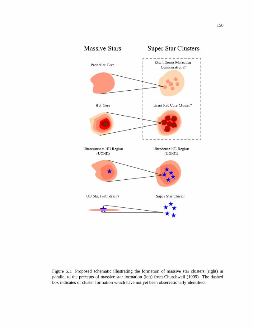
150
Figure 6.1: Proposed schematic illustrating the formation of massive star clusters (right) inparallel to the precepts of massive star formation (left) from Churchwell (1999). The dashedbox indicates of cluster formation which have not yet been observationally identified.
151
6.5 Develop More Sophisticated Models
While the simple models presented in Chapters 4 and 5 are adequate for estimating mean
physical properties, such as density, more sophisticated models would allow us to investigate
the detailed dependence of observable quantities on varying physical conditions. More realistic
models would need to include an arbitrary number of embedded stars (each with its own density
profile and temperature distribution) embedded in a diffuse medium and allowed to evolve in
time. Such models could predict the detailed dependence of observables such as the evolution
of the spectral energy distribution of the enshrouding dust cocoon and the radio spectral index.
6.6 Summary of Future Possibilities
The origin of globular clusters has eluded researchers for many years, possibly because
of the assumption that we would first need to able to observe the early universe in detail in order
to find such objects. However, as we learned in Chapters 1 and 2 of this thesis, many young
massive star clusters have been found with the Hubble Space Telescope in a number of systems,
often in merging galaxies such as the famous Antennae. These clusters had to form somehow,
somewhere in their host galaxies, and the most logical way to look for them is with the same
methods used to find UCHII regions in our galaxy — radio, mm, and possibly in the far-IR.
Indeed, perhaps we can even ask some of the same questions that we ask about UCH II regions.
For example, is maser activity associated with UDH IIs? Do UDH IIs have the same “lifetime
problem”? When stellar winds are established, how do they affect the birth environment? The
first steps in understanding massive star cluster formation will be to catalog a larger sample of
UDH IIs, map out their spectral energy distributions (in so far as current instrumentation will
allow), and determine the physical properties of their birth environments. I look forward to
providing updates on the progress of this reseach to the community in the coming years.

152
Ad astra per aspera
Bibliography
Afflerbach, A., Churchwell, E., Acord, J. M., Hofner, P., Kurtz, S., & Depree, C. G. 1996,ApJS, 106, 423
Allen, D. A., Wright, A. E., & Goss, W. M. 1976, MNRAS, 177, 91
Allen, M. L. & Kronberg, P. P. 1998, ApJ, 502, 218
Anantharamaiah, K. R., Viallefond, F., Mohan, N. R., Goss, W. M., & Zhao, J. H. 2000, ApJ,537, 613
Arendt, R. G. 1989, ApJS, 70, 181
Arp, H. & Sandage, A. 1985, AJ, 90, 1163
Ashman, K. M. & Zepf, S. E. 1992, ApJ, 384, 50
Baas, F., Israel, F. P., & Koornneef, J. 1994, A&A, 284, 403
Balland, C., Silk, J., & Schaeffer, R. 1998, ApJ, 497, 541
Barnes, J. E. 1988, ApJ, 331, 699
—. 1989, Nature, 338, 123
Barnes, J. E. 1997, in ASP Conf. Ser. 116: The Nature of Elliptical Galaxies; 2nd StromloSymposium, 469+
Barnes, J. E. & Hernquist, L. 1992, Nature, 360, 715
—. 1996, ApJ, 471, 115
Barnes, J. E. & Hernquist, L. E. 1991, ApJL, 370, L65
Baron, E. & White, S. D. M. 1987, ApJ, 322, 585
Beck, S. C., Kelly, D. M., & Lacy, J. H. 1997, AJ, 114, 585
Beck, S. C., Turner, J. L., & Kovo, O. 2000, AJ, 120, 244
Bianchi, S., Davies, J. I., Alton, P. B., Gerin, M., & Casoli, F. 2000, A&A, 353, L13
154
Boulesteix, J., Courtes, G., Laval, A., Monnet, G., & Petit, H. 1974, A&A, 37, 33
Burgarella, D. & Chapelon, S. 1998, in ASP Conf. Ser. 133: Science With The NGST, 227
Buta, R., Crocker, D. A., & Byrd, G. G. 1999, AJ, 118, 2071
Calzetti, D., Kinney, A. L., & Storchi-Bergmann, T. 1994, ApJ, 429, 582
Carilli, C. L., Holdaway, M. A., Ho, P. T. P., & de Pree, C. G. 1992, ApJL, 399, L59
Cervino, M. & Mas-Hesse, J. M. 1994, A&A, 284, 749
Chandar, R., Bianchi, L., Ford, H. C., & Salasnich, B. 1999, PASP, 111, 794
Chu, Y. & Kennicutt, R. C. 1994, ApJ, 425, 720
Churchwell, E. 1999, in NATO ASIC Proc. 540: The Origin of Stars and Planetary Systems,515
Clarke, C. J., Bonnell, I. A., & Hillenbrand, L. A. 2000, in Protostars and Planets IV, 151
Cohen, M., Walker, R. G., Carter, B., Hammersley, P., Kidger, M., & Noguchi, K. 1999, AJ,117, 1864
Condon, J. J. 1992, ARA&A, 30, 575
Condon, J. J., Anderson, M. L., & Helou, G. 1991a, ApJ, 376
Condon, J. J., Huang, Z. ., Yin, Q. F., & Thuan, T. X. 1991b, ApJ, 378, 65
Condon, J. J. & Yin, Q. F. 1990, ApJ, 357, 97
Conti, P. S. 1991, ApJ, 377, 115
Conti, P. S. & Blum, R. 2001, ApJ, in press
Conti, P. S., Leitherer, C., & Vacca, W. D. 1996, ApJL, 461, L87
Conti, P. S. & Vacca, W. D. 1994, ApJL, 423, L97
Corbin, M. R., Korista, K. T., & Vacca, W. D. 1993, AJ, 105, 1313
Courtes, G., Petit, H., Petit, M., Sivan, J. P., & Dodonov, S. 1987, A&A, 174, 28
Cowie, L. L., Songaila, A., Kim, T., & Hu, E. M. 1995, AJ, 109, 1522
Crowther, P. A., Beck, S. C., Willis, A. J., Conti, P. S., Morris, P. W., & Sutherland, R. S. 1999,MNRAS, 304, 654
de Grijs, R., O’Connell, R. W., & Gallagher, J. S. 2001, AJ, 121, 768
de Marchi, G., Clampin, M., Greggio, L., Leitherer, C., Nota, A., & Tosi, M. 1997, ApJL, 479,L27
de Pree, C. G., Mehringer, D. M., & Goss, W. M. 1997, ApJ, 482, 307
155
de Pree, C. G., Rodriguez, L. F., & Goss, W. M. 1995, Revista Mexicana de Astronomia yAstrofisica, 31, 39
de Vaucouleurs, G. 1979, ApJ, 227, 729
de Vaucouleurs, G., de Vaucouleurs, A., & Corwin, H. G. 1976, 2nd reference catalogue ofbright galaxies containing information on 4364 galaxies with reference to papers publishedbetween 1964 and 1975 (University of Texas Monographs in Astronomy, Austin: Universityof Texas Press, 1976)
Dove, J. B., Shull, J. M., & Ferrara, A. 2000, ApJ, 531, 846
Duc, P. . & Mirabel, I. F. 1994, A&A, 289, 83
Duric, N., Viallefond, F., Goss, W. M., & van der Hulst, J. M. 1993, A&AS, 99, 217
Elmegreen, B. G., Efremov, Y., Pudritz, R. E., & Zinnecker, H. 2000a, in Protostars and PlanetsIV, 179
Elmegreen, B. G. & Efremov, Y. N. 1997, ApJ, 480, 235
Elmegreen, B. G., Efremov, Y. N., & Larsen, S. 2000b, ApJ, 535, 748
Elmegreen, B. G., Kaufman, M., & Thomasson, M. 1993, ApJ, 412, 90
Elmegreen, D. M., Kaufman, M., Brinks, E., Elmegreen, B. G., & Sundin, M. 1995, ApJ, 453,100
Fabian, A. C. 1994, ARA&A, 32, 277
Ferrara, A. & Tolstoy, E. 2000, MNRAS, 313, 291
Figer, D. F., Kim, S. S., Morris, M., Serabyn, E., Rich, R. M., & McLean, I. S. 1999, ApJ, 525,750
Filipovic, M. D., Haynes, R. F., White, G. L., Jones, P. A., Klein, U., & Wielebinski, R. 1995,A&AS, 111, 311
Filipovic, M. D., Jones, P. A., White, G. L., & Haynes, R. F. 1998, A&AS, 130, 441
Filipovic, M. D., Jones, P. A., White, G. L., Haynes, R. F., Klein, U., & Wielebinski, R. 1997,A&AS, 121, 321
Forbes, D. A. & Hau, G. K. T. 2000, MNRAS, 312, 703
Freedman, W. L., Hughes, S. M., Madore, B. F., Mould, J. R., Lee, M. G., Stetson, P., Kennicutt,R. C., Turner, A., Ferrarese, L., Ford, H., Graham, J. A., Hill, R., Hoessel, J. G., Huchra, J.,& Illingworth, G. D. 1994, ApJ, 427, 628
Freedman, W. L., Wilson, C. D., & Madore, B. F. 1991, ApJ, 372, 455
Gallagher, J. S., Hunter, D. A., & Tutukov, A. V. 1984, ApJ, 284, 544
Garcia-Gomez, C. & Athanassoula, E. 1991, A&AS, 89, 159

156
Gonzalez Delgado, R. M., Leitherer, C., Heckman, T., Lowenthal, J. D., Ferguson, H. C., &Robert, C. 1998, ApJ, 495, 698
Gordon, S. M., Duric, N., Kirshner, R. P., Goss, W. M., & Viallefond, F. 1999, ApJS, 120, 247
Gorjian, V., Turner, J. L., & Beck, S. C. 2001, AJ, in press
Gwinn, C. R., Moran, J. M., & Reid, M. J. 1992, ApJ, 393, 149
Harris, W. E. 1991, ARA&A, 29, 543
Harris, W. E. & Pudritz, R. E. 1994, ApJ, 429, 177
Heckman, T. M. 1997, in Star Formation Near and Far, 271
Heckman, T. M. 1998, in ASP Conf. Ser. 148: Origins, 127
Heckman, T. M. 2001, in ASP Conf. Ser.: Gas and Galaxy Evolution, in press
Heckman, T. M., Dahlem, M., Lehnert, M. D., Fabbiano, G., Gilmore, D., & Waller, W. H.1995, ApJ, 448, 98
Henize, K. G. 1967, ApJS, 14, 125
Hernquist, L. 1992, ApJ, 400, 460
—. 1993, ApJ, 409, 548
Hernquist, L. & Spergel, D. N. 1992, ApJL, 399, L117
Hibbard, J. E. & Vacca, W. D. 1997, AJ, 114, 1741
Hickson, P. 1982, ApJ, 255, 382
Hickson, P., Mendes de Oliveira, C., Huchra, J. P., & Palumbo, G. G. 1992, ApJ, 399, 353
Hickson, P., Richstone, D. O., & Turner, E. L. 1977, ApJ, 213, 323
Hills, J. G. 1980, ApJ, 235, 986
Ho, L. C. & Filippenko, A. V. 1996a, ApJL, 466, L83
—. 1996b, ApJ, 472, 600
Hodge, P. W., Balsley, J., Wyder, T. K., & Skelton, B. P. 1999, PASP, 111, 685
Hollenbach, D., Johnstone, D., Lizano, S., & Shu, F. 1994, ApJ, 428, 654
Holtzman, J. A., Burrows, C. J., Casertano, S., Hester, J. J., Trauger, J. T., Watson, A. M., &Worthey, G. 1995a, PASP, 107, 1065
Holtzman, J. A., Faber, S. M., Shaya, E. J., Lauer, T. R., Grothe, J., Hunter, D. A., Baum, W. A.,Ewald, S. P., Hester, J. F., Light, R. M., Lynds, C. R., O’Neil, E. J., & Westphal, J. A. 1992,AJ, 103, 691
157
Holtzman, J. A., Hester, J. J., Casertano, S., Trauger, J. T., Watson, A. M., Ballester, G. E.,Burrows, C. J., Clarke, J. T., Crisp, D., Evans, R. W., Gallagher, J. S., Griffiths, R. E.,Hoessel, J. G., Matthews, L. D., Mould, J. R., Scowen, P. A., Stapelfeldt, K. R., & Westphal,J. A. 1995b, PASP, 107, 156
Hunsberger, S. D., Charlton, J. C., & Zaritsky, D. 1996, ApJ, 462, 50+
—. 1998, ApJ, 505, 536
Hutsemekers, D. & Surdej, J. 1984, A&A, 133, 209
Hyman, S. D., Lacey, C. K., Weiler, K. W., & Van Dyk, S. D. 2000, AJ, 119, 1711
Iglesias-Paramo, J. & Vilchez, J. M. 1997, ApJ, 479, 190
Jenkins, E. B., Jura, M., & Loewenstein, M. 1983, ApJ, 270, 88
Johansson, I. 1987, A&A, 182, 179
Johnson, K. E., Leitherer, C., Vacca, W. D., & Conti, P. S. 2000, AJ, 120, 1273
Johnson, K. E., Vacca, W. D., Leitherer, C., Conti, P. S., & Lipscy, S. J. 1999, AJ, 117, 1708
Kawara, K., Nishida, M., & Phillips, M. M. 1989, ApJ, 337, 230
Kellermann, K. I., Sramek, R., Schmidt, M., Shaffer, D. B., & Green, R. 1989, AJ, 98, 1195
Kennicutt, R. C. 1984, ApJ, 287, 116
—. 1998, ApJ, 498, 541
Keto, E., Hora, J. L., Fazio, G. G., Hoffmann, W., & Deutsch, L. 1999, ApJ, 518, 183
Kim, S. S., Morris, M., & Lee, H. M. 1999, ApJ, 525, 228
Kobulnicky, H. A., Dickey, J. M., Sargent, A. I., Hogg, D. E., & Conti, P. S. 1995, AJ, 110, 116
Kobulnicky, H. A. & Johnson, K. E. 1999, ApJ, 527, 154
Kobulnicky, H. A., Kennicutt, R. C., & Pizagno, J. L. 1999, ApJ, 514, 544
Kobulnicky, H. A., Skillman, E. D., Roy, J., Walsh, J. R., & Rosa, M. R. 1997, ApJ, 477, 679
Kolatt, T. S., Bullock, J. S., Somerville, R. S., Sigad, Y., Jonsson, P., Kravtsov, A. V., Klypin,A. A., Primack, J. R., Faber, S. M., & Dekel, A. 1999, ApJL, 523, L109
Krist, J. 1993, in ASP Conf. Ser. 52: Astronomical Data Analysis Software and Systems II,Vol. 2, 536
Kuehr, H., Witzel, A., Pauliny-Toth, I. I. K., & Nauber, U. 1981, A&AS, 45, 367
Kunth, D., Mas-Hesse, J. M., Terlevich, E., Terlevich, R., Lequeux, J., & Fall, S. M. 1998,A&A, 334, 11
Kunth, D. & Schild, H. 1986, A&A, 169, 71
158
Kurtz, S., Cesaroni, R., Churchwell, E., Hofner, P., & Walmsley, C. M. 2000, in Protostars andPlanets IV, 299
Lacey, C., Duric, N., & Goss, W. M. 1997, ApJS, 109, 417
Larsen, S. S. & Richtler, T. 1999, A&A, 345, 59
Lasker, B. M., Sturch, C. R., McLean, B. J., Russell, J. L., Jenkner, H., & Shara, M. M. 1990,AJ, 99, 2019
Leitherer, C. & Heckman, T. M. 1995, ApJS, 96, 9
Leitherer, C., Robert, C., & Heckman, T. M. 1995, ApJS, 99, 173
Leitherer, C., Schaerer, D., Goldader, J. D., Delgado, R. M. G., Robert, C., Kune, D. F., deMello, D. F., Devost, D., & Heckman, T. M. 1999, ApJS, 123, 3
Lowenthal, J. D., Koo, D. C., Guzman, R., Gallego, J., Phillips, A. C., Faber, S. M., Vogt, N. P.,Illingworth, G. D., & Gronwall, C. 1997, ApJ, 481, 673
Mendez, D. I., Esteban, C., Filipovic , M. D., Ehle, M., Haberl, F., Pietsch, W., & Haynes, R. F.1999, A&A, 349, 801
Mac Low, M. & Ferrara, A. 1999, ApJ, 513, 142
Madau, P., Haardt, F., & Rees, M. J. 1999, ApJ, 514, 648
Madau, P. & Shull, J. M. 1996, ApJ, 457, 551+
Madden, S. C. 2000, New Astronomy Review, 44, 249
Maeder, A. & Conti, P. S. 1994, ARA&A, 32, 227
Marlowe, A. T., Heckman, T. M., Wyse, R. F. G., & Schommer, R. 1995, ApJ, 438, 563
Massey, P., Bianchi, L., Hutchings, J. B., & Stecher, T. P. 1996, ApJ, 469, 629
Massey, P. & Hunter, D. A. 1998, ApJ, 493, 180
Massey, P., Johnson, K. E., & Degioia-Eastwood, K. 1995, ApJ, 454, 151
McKee, C. F. & Williams, J. P. 1997, ApJ, 476, 144
Meurer, G. R., Freeman, K. C., Dopita, M. A., & Cacciari, C. 1992, AJ, 103, 60
Meurer, G. R., Heckman, T. M., Lehnert, M. D., Leitherer, C., & Lowenthal, J. 1997, AJ, 114,54
Meurer, G. R., Heckman, T. M., Leitherer, C., Kinney, A., Robert, C., & Garnett, D. R. 1995,AJ, 110, 2665
Meylan, G. 1993, in ASP Conf. Ser. 48: The Globular Cluster-Galaxy Connection, 588+
Mezger, P. G. & Henderson, A. P. 1967, ApJ, 147, 471
159
Mezger, P. G., Schraml, J., & Terzian, Y. 1967, ApJ, 150, 807
Mihos, J. C. & Hernquist, L. 1996, ApJ, 464, 641
Miller, B. W., Whitmore, B. C., Schweizer, F., & Fall, S. M. 1997, AJ, 114, 2381
Mirabel, I. F., Dottori, H., & Lutz, D. 1992, A&A, 256, L19
Mirabel, I. F., Lutz, D., & Maza, J. 1991, A&A, 243, 367
Mohan, N., Anantharamaiah, K., & Goss, W. 2001, ApJ
Nagar, N. M., Falcke, H., Wilson, A. S., & Ho, L. C. 2000, ApJ, 542, 186
O’Connell, R. W., Gallagher, J. S., Hunter, D. A., & Colley, W. N. 1995, ApJL, 446, L1
Pettini, M., Steidel, C. C., Adelberger, K. L., Dickinson, M., & Giavalisco, M. 2000, ApJ, 528,96
Phillips, M. M., Aitken, D. K., & Roche, P. F. 1984, MNRAS, 207, 25
Rubin, V. C., Hunter, D. A., & Ford, W. K. J. 1990, ApJ, 365, 86
Sandage, A., Saha, A., Tammann, G. A., Labhardt, L., Schwengeler, H., Panagia, N., & Mac-chetto, F. D. 1994, ApJL, 423, L13
Sandage, A. & Tammann, G. A. 1981, A revised Shapley-Ames Catalog of bright galaxies(Washington: Carnegie Institution, 1981, Preliminary version)
Sanders, D. B. & Mirabel, I. F. 1996, ARA&A, 34, 749
Sargent, A. & Scoville, N. 1991, ApJL, 366, L1
Sargent, W. L. W. & Searle, L. 1970, ApJL, 162, L155
Sauvage, M., Thuan, T. X., & Lagage, P. O. 1997, A&A, 325, 98
Schaerer, D., Contini, T., & Kunth, D. 1999a, A&A, 341, 399
Schaerer, D., Contini, T., & Pindao, M. 1999b, A&AS, 136, 35
Schlegel, D. J., Finkbeiner, D. P., & Davis, M. 1998, ApJ, 500, 525
Schweizer, F. 1982, ApJ, 252, 455
Schweizer, F., Miller, B. W., Whitmore, B. C., & Fall, S. M. 1996, AJ, 112, 1839
Schwering, P. B. W. & Israel, F. P. 1990, Atlas and catalogue of infrared sources in the Magel-lanic Clouds (Dordrecht: Kluwer, 1990, edited by Schwering, P.B.W.; Israel, F.P.)
Secker, J. 1992, AJ, 104, 1472
Selman, F., Melnick, J., Bosch, G., & Terlevich, R. 1999, A&A, 347, 532
Shu, F. H. 1991, The physics of astrophysics. Vol.1: Radiation (A Series of Books in Astronomy,Mill Valley, CA: University Science Books, 1991)
160
Sirianni, M., Nota, A., Leitherer, C., De Marchi, G., & Clampin, M. 2000, ApJ, 533, 203
Smith, L. F., Mezger, P. G., & Biermann, P. 1978, A&A, 66, 65
Smith, L. J. & Gallagher, J. S. 2001, MNRAS
Smith, T. R. & Kennicutt, R. C. 1989, PASP, 101, 649
Sohn, Y. & Davidge, T. J. 1996, AJ, 112, 2559
Soifer, B. T., Boehmer, L., Neugebauer, G., & Sanders, D. B. 1989, AJ, 98, 766
Steidel, C. C., Giavalisco, M., Pettini, M., Dickinson, M., & Adelberger, K. L. 1996, ApJL,462, L17
Sugai, H. & Taniguchi, Y. 1992, AJ, 103, 1470
Takahashi, K. & Portegies Zwart, S. F. 2000, ApJ, 535, 759
Tarchi, A., Neininger, N., Greve, A., Klein, U., Garrington, S. T., Muxlow, T. W. B., Pedlar, A.,& Glendenning, B. E. 2000, A&A, 358, 95
Telesco, C. M., Dressel, L. L., & Wolstencroft, R. D. 1993, ApJ, 414, 120
Tokunaga, A. T. 1984, AJ, 89, 172
Toomre, A. 1964, ApJ, 139, 1217
Tumlinson, J., Giroux, M. L., Shull, J. M., & Stocke, J. T. 1999, AJ, 118, 2148
Turner, J. L., Beck, S. C., & Ho, P. T. P. 2000, ApJL, 532, L109
Turner, J. L. & Ho, P. T. P. 1985, ApJL, 299, L77
Turner, J. L., Ho, P. T. P., & Beck, S. C. 1998, AJ, 116, 1212
Ulvestad, J. S. & Antonucci, R. R. J. 1997, ApJ, 488, 621
Urry, C. M. & Padovani, P. 1995, PASP, 107, 803
Vacca, W. D. 1994, ApJ, 421, 140
Vacca, W. D. 1997, in The Ultraviolet Universe at Low and High Redshift: Probing the Progressof Galaxy Evolution, 21
Vacca, W. D. & Conti, P. S. 1992, ApJ, 401, 543
Vacca, W. D., Garmany, C. D., & Shull, J. M. 1996, ApJ, 460, 914
Vacca, W. D., Robert, C., Leitherer, C., & Conti, P. S. 1995, ApJ, 444, 647
van Breugel, W. J. M., Stanford, S. A., Spinrad, H., Stern, D., & Graham, J. R. 1998, ApJ, 502,614
van den Bergh, S. 1971, A&A, 12, 474
161
—. 1995, Nature, 374, 215
van der Kruit, P. C. 1971, A&A, 15, 110
Vanhala, H. A. T. & Cameron, A. G. W. 1998, ApJ, 508, 291
Venkatesan, A., Giroux, M. L., & Shull, J. M. 2001, ApJ
Verschueren, W. 1990, A&A, 234, 156
Ward-Thompson, D. & Robson, E. I. 1990, MNRAS, 244, 458
Watson, A. M., Gallagher, J. S., Holtzman, J. A., Hester, J. J., Mould, J. R., Ballester, G. E.,Burrows, C. J., Casertano, S., Clarke, J. T., Crisp, D., Evans, R., Griffiths, R. E., Hoessel,J. G., Scowen, P. A., Stapelfeldt, K. R., Trauger, J. T., & Westphtptphal, J. A. 1996, AJ, 112,534
Weiler, K. W. & Panagia, N. 1978, A&A, 70, 419
Weiler, K. W., Sramek, R. A., Panagia, N., van der Hulst, J. M., & Salvati, M. 1986, ApJ, 301,790
Whitmore, B. 2000, in ASP Conf. Ser. 197: Dynamics of Galaxies: from the Early Universe tothe Present, 315
Whitmore, B. C. 1999, in IAU Symp. 186: Galaxy Interactions at Low and High Redshift, Vol.186, 251
Whitmore, B. C. & Schweizer, F. 1995, AJ, 109, 960
Whitmore, B. C., Schweizer, F., Leitherer, C., Borne, K., & Robert, C. 1993, AJ, 106, 1354
Whitmore, B. C., Zhang, Q., Leitherer, C., Fall, S. M., Schweizer, F., & Miller, B. W. 1999, AJ,118, 1551
Williams, B. A., McMahon, P. M., & van Gorkom, J. H. 1991, AJ, 101, 1957
Williams, R. E., Blacker, B., Dickinson, M., Dixon, W. V. D., Ferguson, H. C., Fruchter, A. S.,Giavalisco, M., Gilliland, R. L., Heyer, I., Katsanis, R., Levay, Z., Lucas, R. A., McElroy,D. B., Petro, L., Postman, M., Adorf, H., & Hook, R. 1996, AJ, 112, 1335
Wood, D. O. S. & Churchwell, E. 1989a, ApJ, 340, 265
—. 1989b, ApJS, 69, 831
Woosley, S. E. & Weaver, T. A. 1995, ApJS, 101, 181
Wray, J. D. 1988, The color atlas of galaxies (Research supported by NSF,. Cambridge andNew York, Cambridge University Press, 1988, 201 p.)
Zepf, S. E., Ashman, K. M., English, J., Freeman, K. C., & Sharples, R. M. 1999, AJ, 118, 752
Zhang, Q., Fall, S. M., & Whitmore, B. C. 2000, in American Astronomical Society Meeting,Vol. 197, 2406
Appendix A
UCH II Candidates in the Magellanic Clouds
In the Galaxy, UCH IIs have been identified by their thermal radio spectra and their
IRAS colors. Just as the UDH IIs discussed in Chapters 4 and 5 have flat or inverted radio
spectra at cm wavelengths, individual UCH IIs are expected to have thermal radio spectral en-
ergy distributions as well. However, in the catalog of UCH II regions by Wood & Church-
well (1989b), many of the UCH II regions have radio spectral indices consistent with optically
thin thermal free-free emission. Wood & Churchwell (1989a) also found that UCH IIs in the
Galaxy strictly obey a set of color criteria in the infrared with � � � � � � �� � � � � �� � � � � and
� � � � � � �� � � � � �� � � � � , while very few other types of objects had IRAS colors fitting these
criteria. For example, in the sample of Arendt (1989), none of the SNR meet both of these crite-
ria. Therefore, these color criteria appear to be relatively robust for identifying UCH II regions.
Wood & Churchwell (1989b) also note that 60% of the brightest IRAS sources ( � � � � Jy at
100 � m) in the range of their survey are UCH II regions. Therefore, we expect UCH II regions
to be among the brightest mid- to far-infrared sources in the Magellanic Clouds.
The radio observations used in this appendix were originally obtained by Filipovic et al.
(1995, 1997) using the Parkes radio telescope. The beamsize at the frequencies used here are
3.6 arcmin at 8.85 GHz, 5.2 arcmin at 4.85 GHz, and 5.6 at 4.75 GHz. These beamsizes are
large compared to the expected size of a UCH II region in the Magellanic Clouds of � � � � � arc-
sec. Consequently, these observations are likely to suffer from severe contamination by other
radio emitting objects and background radio continuum. The RMS noise for these frequencies
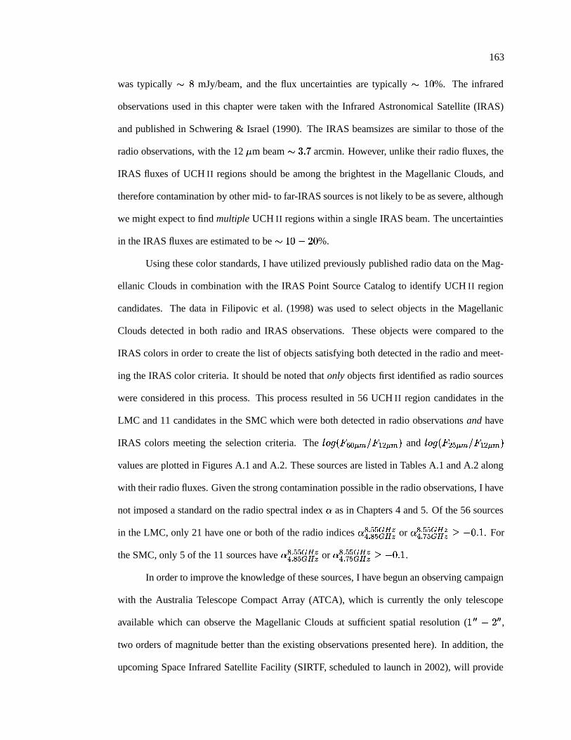
163
was typically � � mJy/beam, and the flux uncertainties are typically � � � %. The infrared
observations used in this chapter were taken with the Infrared Astronomical Satellite (IRAS)
and published in Schwering & Israel (1990). The IRAS beamsizes are similar to those of the
radio observations, with the 12 � m beam � � � � arcmin. However, unlike their radio fluxes, the
IRAS fluxes of UCH II regions should be among the brightest in the Magellanic Clouds, and
therefore contamination by other mid- to far-IRAS sources is not likely to be as severe, although
we might expect to find multiple UCH II regions within a single IRAS beam. The uncertainties
in the IRAS fluxes are estimated to be � � � � � � %.
Using these color standards, I have utilized previously published radio data on the Mag-
ellanic Clouds in combination with the IRAS Point Source Catalog to identify UCH II region
candidates. The data in Filipovic et al. (1998) was used to select objects in the Magellanic
Clouds detected in both radio and IRAS observations. These objects were compared to the
IRAS colors in order to create the list of objects satisfying both detected in the radio and meet-
ing the IRAS color criteria. It should be noted that only objects first identified as radio sources
were considered in this process. This process resulted in 56 UCH II region candidates in the
LMC and 11 candidates in the SMC which were both detected in radio observations and have
IRAS colors meeting the selection criteria. The � � � � � � �� � � � � � and � � � � � � �� � � � � �values are plotted in Figures A.1 and A.2. These sources are listed in Tables A.1 and A.2 along
with their radio fluxes. Given the strong contamination possible in the radio observations, I have
not imposed a standard on the radio spectral index � as in Chapters 4 and 5. Of the 56 sources
in the LMC, only 21 have one or both of the radio indices � � � � � ���� � � � ��� or � � � � � ���� � � � ���� � � � � . For
the SMC, only 5 of the 11 sources have � � � � � ���� � � � ��� or � � � � � ���� � � � ���� � � � � .
In order to improve the knowledge of these sources, I have begun an observing campaign
with the Australia Telescope Compact Array (ATCA), which is currently the only telescope
available which can observe the Magellanic Clouds at sufficient spatial resolution ( � � � ��� � � ,two orders of magnitude better than the existing observations presented here). In addition, the
upcoming Space Infrared Satellite Facility (SIRTF, scheduled to launch in 2002), will provide

164
higher resolution mid- to far-infrared data on these sources.
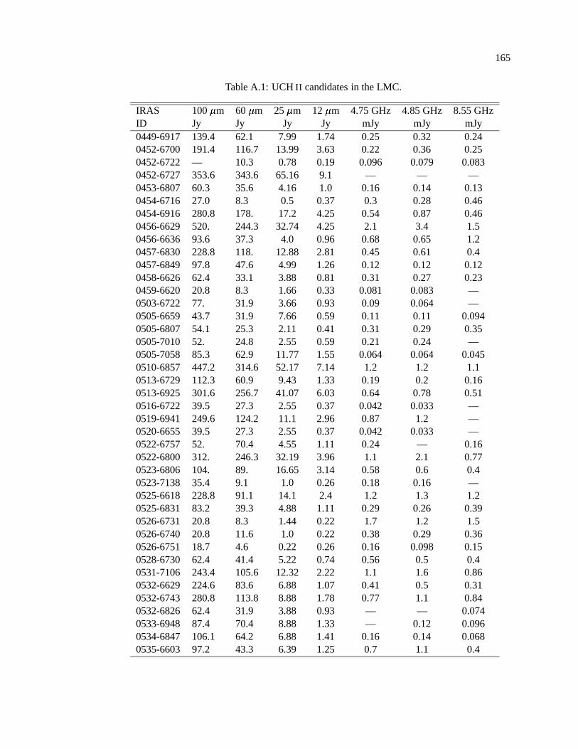
165
Table A.1: UCH II candidates in the LMC.
IRAS 100 � m 60 � m 25 � m 12 � m 4.75 GHz 4.85 GHz 8.55 GHzID Jy Jy Jy Jy mJy mJy mJy0449-6917 139.4 62.1 7.99 1.74 0.25 0.32 0.240452-6700 191.4 116.7 13.99 3.63 0.22 0.36 0.250452-6722 — 10.3 0.78 0.19 0.096 0.079 0.0830452-6727 353.6 343.6 65.16 9.1 — — —0453-6807 60.3 35.6 4.16 1.0 0.16 0.14 0.130454-6716 27.0 8.3 0.5 0.37 0.3 0.28 0.460454-6916 280.8 178. 17.2 4.25 0.54 0.87 0.460456-6629 520. 244.3 32.74 4.25 2.1 3.4 1.50456-6636 93.6 37.3 4.0 0.96 0.68 0.65 1.20457-6830 228.8 118. 12.88 2.81 0.45 0.61 0.40457-6849 97.8 47.6 4.99 1.26 0.12 0.12 0.120458-6626 62.4 33.1 3.88 0.81 0.31 0.27 0.230459-6620 20.8 8.3 1.66 0.33 0.081 0.083 —0503-6722 77. 31.9 3.66 0.93 0.09 0.064 —0505-6659 43.7 31.9 7.66 0.59 0.11 0.11 0.0940505-6807 54.1 25.3 2.11 0.41 0.31 0.29 0.350505-7010 52. 24.8 2.55 0.59 0.21 0.24 —0505-7058 85.3 62.9 11.77 1.55 0.064 0.064 0.0450510-6857 447.2 314.6 52.17 7.14 1.2 1.2 1.10513-6729 112.3 60.9 9.43 1.33 0.19 0.2 0.160513-6925 301.6 256.7 41.07 6.03 0.64 0.78 0.510516-6722 39.5 27.3 2.55 0.37 0.042 0.033 —0519-6941 249.6 124.2 11.1 2.96 0.87 1.2 —0520-6655 39.5 27.3 2.55 0.37 0.042 0.033 —0522-6757 52. 70.4 4.55 1.11 0.24 — 0.160522-6800 312. 246.3 32.19 3.96 1.1 2.1 0.770523-6806 104. 89. 16.65 3.14 0.58 0.6 0.40523-7138 35.4 9.1 1.0 0.26 0.18 0.16 —0525-6618 228.8 91.1 14.1 2.4 1.2 1.3 1.20525-6831 83.2 39.3 4.88 1.11 0.29 0.26 0.390526-6731 20.8 8.3 1.44 0.22 1.7 1.2 1.50526-6740 20.8 11.6 1.0 0.22 0.38 0.29 0.360526-6751 18.7 4.6 0.22 0.26 0.16 0.098 0.150528-6730 62.4 41.4 5.22 0.74 0.56 0.5 0.40531-7106 243.4 105.6 12.32 2.22 1.1 1.6 0.860532-6629 224.6 83.6 6.88 1.07 0.41 0.5 0.310532-6743 280.8 113.8 8.88 1.78 0.77 1.1 0.840532-6826 62.4 31.9 3.88 0.93 — — 0.0740533-6948 87.4 70.4 8.88 1.33 — 0.12 0.0960534-6847 106.1 64.2 6.88 1.41 0.16 0.14 0.0680535-6603 97.2 43.3 6.39 1.25 0.7 1.1 0.4
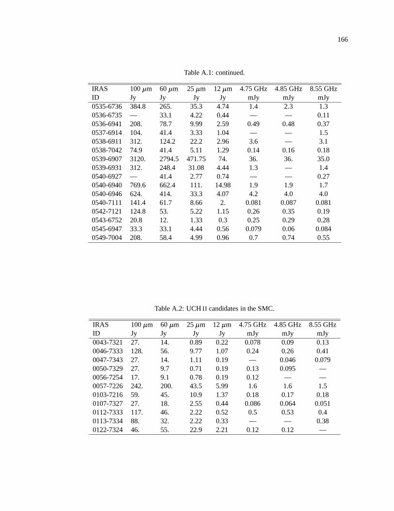
166
Table A.1: continued.
IRAS 100 � m 60 � m 25 � m 12 � m 4.75 GHz 4.85 GHz 8.55 GHzID Jy Jy Jy Jy mJy mJy mJy0535-6736 384.8 265. 35.3 4.74 1.4 2.3 1.30536-6735 — 33.1 4.22 0.44 — — 0.110536-6941 208. 78.7 9.99 2.59 0.49 0.48 0.370537-6914 104. 41.4 3.33 1.04 — — 1.50538-6911 312. 124.2 22.2 2.96 3.6 — 3.10538-7042 74.9 41.4 5.11 1.29 0.14 0.16 0.180539-6907 3120. 2794.5 471.75 74. 36. 36. 35.00539-6931 312. 248.4 31.08 4.44 1.3 — 1.40540-6927 — 41.4 2.77 0.74 — — 0.270540-6940 769.6 662.4 111. 14.98 1.9 1.9 1.70540-6946 624. 414. 33.3 4.07 4.2 4.0 4.00540-7111 141.4 61.7 8.66 2. 0.081 0.087 0.0810542-7121 124.8 53. 5.22 1.15 0.26 0.35 0.190543-6752 20.8 12. 1.33 0.3 0.25 0.29 0.280545-6947 33.3 33.1 4.44 0.56 0.079 0.06 0.0840549-7004 208. 58.4 4.99 0.96 0.7 0.74 0.55
Table A.2: UCH II candidates in the SMC.
IRAS 100 � m 60 � m 25 � m 12 � m 4.75 GHz 4.85 GHz 8.55 GHzID Jy Jy Jy Jy mJy mJy mJy0043-7321 27. 14. 0.89 0.22 0.078 0.09 0.130046-7333 128. 56. 9.77 1.07 0.24 0.26 0.410047-7343 27. 14. 1.11 0.19 — 0.046 0.0790050-7329 27. 9.7 0.71 0.19 0.13 0.095 —0056-7254 17. 9.1 0.78 0.19 0.12 — —0057-7226 242. 200. 43.5 5.99 1.6 1.6 1.50103-7216 59. 45. 10.9 1.37 0.18 0.17 0.180107-7327 27. 18. 2.55 0.44 0.086 0.064 0.0510112-7333 117. 46. 2.22 0.52 0.5 0.53 0.40113-7334 88. 32. 2.22 0.33 — — 0.380122-7324 46. 55. 22.9 2.21 0.12 0.12 —
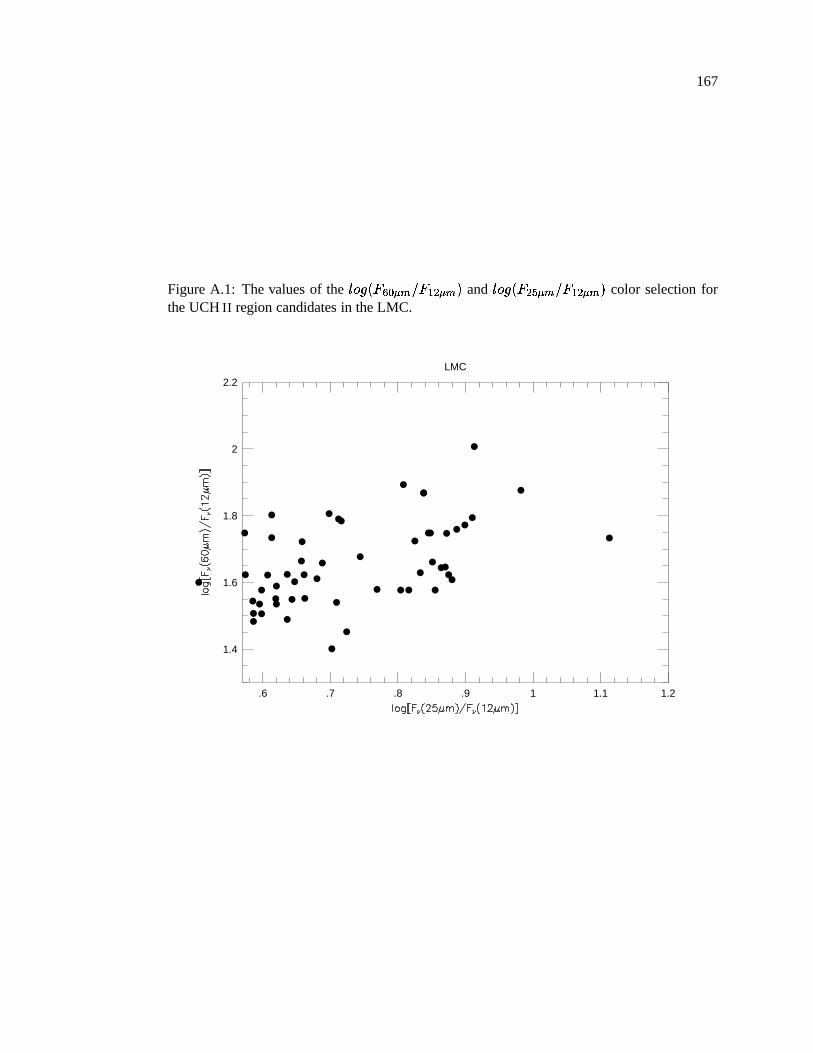
167
Figure A.1: The values of the � � � � � � � � � � � � and � � � � � � � � � � � � color selection forthe UCH II region candidates in the LMC.
.6 .7 .8 .9 1 1.1 1.2
1.4
1.6
1.8
2
2.2
LMC
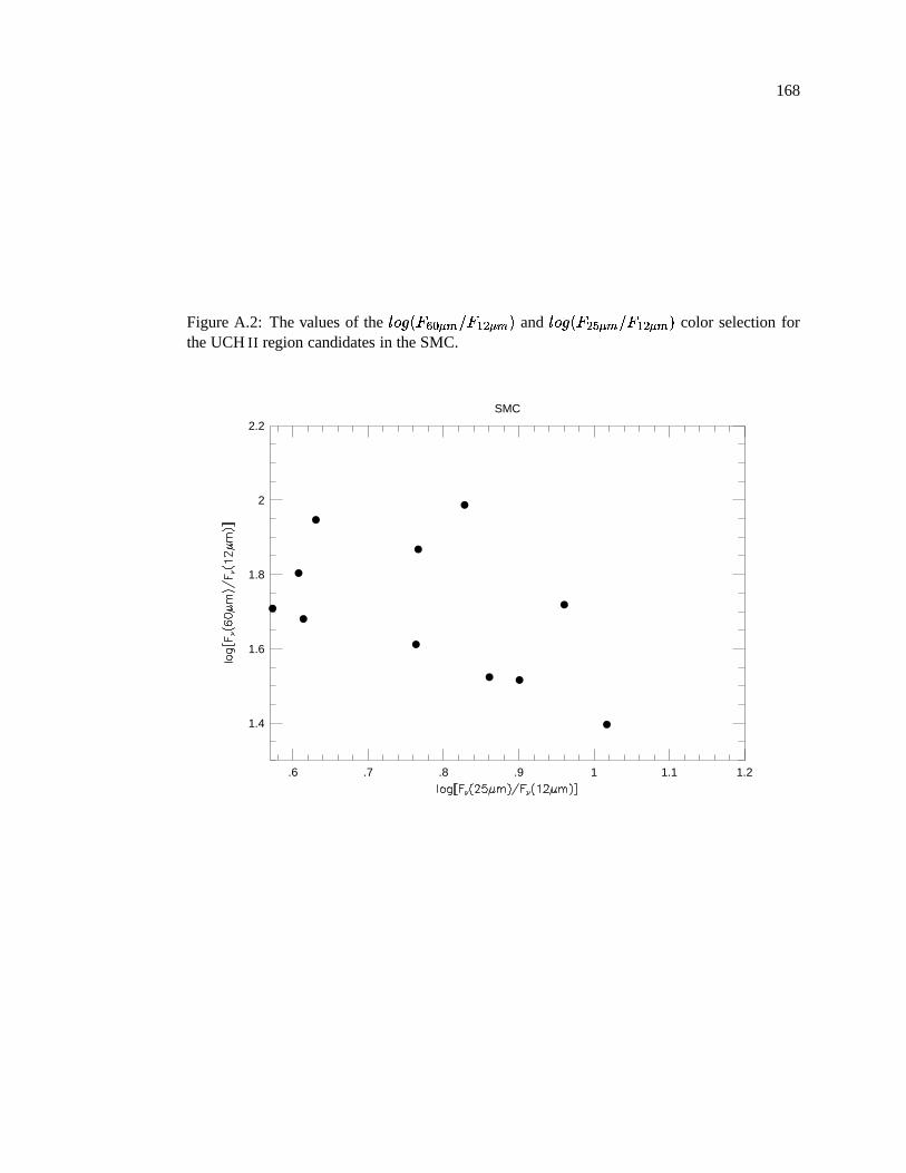
168
Figure A.2: The values of the � � � � � � � � � � � � and � � � � � � � � � � � � color selection forthe UCH II region candidates in the SMC.
.6 .7 .8 .9 1 1.1 1.2
1.4
1.6
1.8
2
2.2
SMC