The Problem of OverfittingThe Problem of Overfitting

BR data: neural network with 20% classification noise, 307 training examples

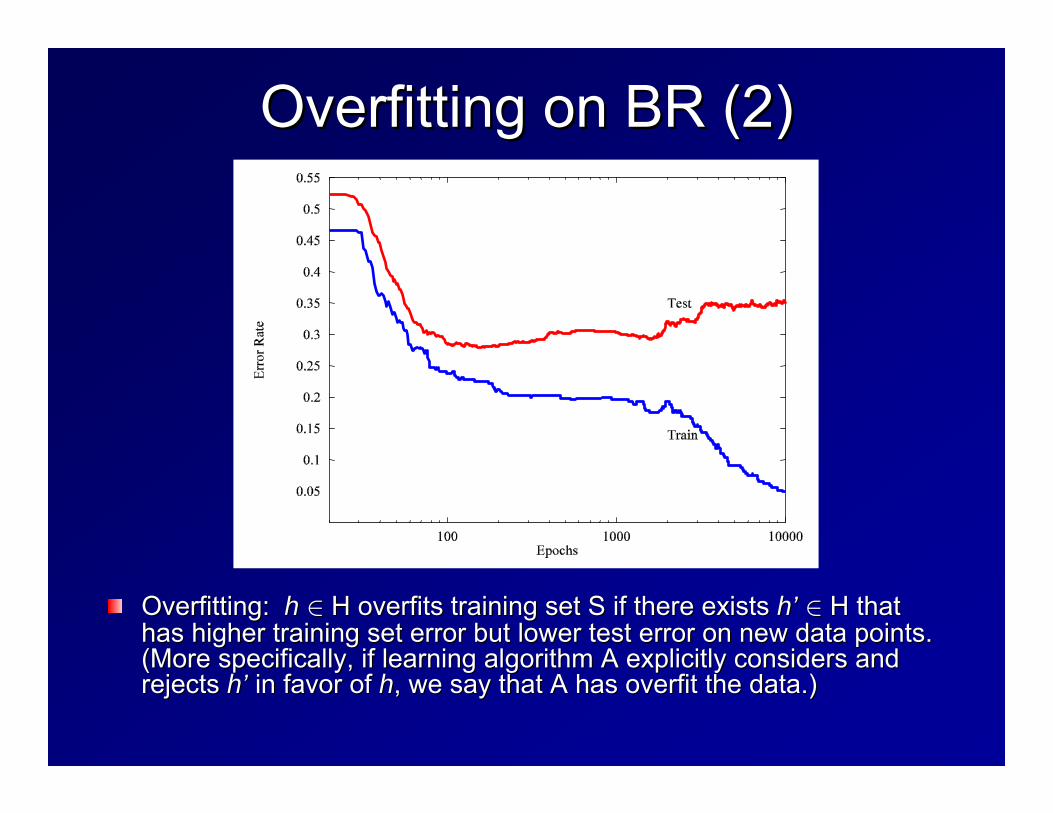
Overfitting on BR (2)Overfitting on BR (2)

Overfitting: Overfitting: hh ∈∈ H overfits training set S if there exists H overfits training set S if there exists hh’’ ∈∈ H that H that has higher training set error but lower test error on new data phas higher training set error but lower test error on new data points. oints. (More specifically, if learning algorithm A explicitly considers(More specifically, if learning algorithm A explicitly considers and and rejects rejects hh’’ in favor of in favor of hh, we say that A has overfit the data.), we say that A has overfit the data.)

OverfittingOverfitting

If we use an hypothesis space HIf we use an hypothesis space Hii that is too large, that is too large, eventually we can trivially fit the training data. In other eventually we can trivially fit the training data. In other words, the VC dimension will eventually be equal to the words, the VC dimension will eventually be equal to the size of our training sample size of our training sample mm..This is sometimes called This is sometimes called ““model selectionmodel selection””, because we , because we can think of each Hcan think of each Hii as an alternative as an alternative ““modelmodel”” of the dataof the data

H1 ⊂ H2 ⊂ H3 ⊂L

Approaches to Preventing Approaches to Preventing OverfittingOverfitting

Penalty methodsPenalty methods–– MAP provides a penalty based on P(H)MAP provides a penalty based on P(H)–– Structural Risk MinimizationStructural Risk Minimization–– Generalized CrossGeneralized Cross--validationvalidation–– AkaikeAkaike’’s Information Criterion (AIC)s Information Criterion (AIC)

Holdout and CrossHoldout and Cross--validation methodsvalidation methods–– Experimentally determine when overfitting occursExperimentally determine when overfitting occurs

EnsemblesEnsembles–– Full Bayesian methods vote many hypotheses Full Bayesian methods vote many hypotheses ∑∑hh P(y|P(y|xx,h) P(h|S),h) P(h|S)

–– Many practical ways of generating ensemblesMany practical ways of generating ensembles

Penalty methodsPenalty methodsLet Let εεtraintrain be our training set error and be our training set error and εεtesttest be our test be our test error. Our real goal is to find the error. Our real goal is to find the hh that minimizes that minimizes εεtesttest. . The problem is that we canThe problem is that we can’’t directly evaluate t directly evaluate εεtesttest. We . We can measure can measure εεtraintrain, but it is optimistic, but it is optimisticPenalty methods attempt to find some penalty such thatPenalty methods attempt to find some penalty such that

εεtesttest = = εεtraintrain + penalty+ penalty

The penalty term is also called a The penalty term is also called a regularizerregularizer or or regularization termregularization term..During training, we set our objective function J to beDuring training, we set our objective function J to be

J(J(ww) = ) = εεtraintrain((ww) + penalty() + penalty(ww))

and find the and find the ww to minimize this functionto minimize this function

MAP penaltiesMAP penaltieshhmapmap = argmax= argmaxhh P(S|h) P(h)P(S|h) P(h)

As As hh becomes more complex, we can assign it a lower becomes more complex, we can assign it a lower prior probability. A typical approach is to assign equal prior probability. A typical approach is to assign equal probability to each of the nested hypothesis spaces so probability to each of the nested hypothesis spaces so thatthat

P(h P(h ∈∈ HH11) = P(h ) = P(h ∈∈ HH22) = ) = LL = = ααBecause HBecause H22 contains more hypotheses than Hcontains more hypotheses than H11, each , each individual h individual h ∈∈ HH22 will have lower prior probability:will have lower prior probability:

P(h) = P(h) = ∑∑ii P(h P(h ∈∈ HHii) = ) = ∑∑ii αα/|H/|Hii| for each i where h | for each i where h ∈∈ HHii

If there are infinitely many Hi, this will not work, because the probabilities must sum to 1. In this case, a common approach is

P(h) = ∑i 2-i/|Hi| for each i where h ∈ Hi

This is not usually a big enough penalty to prevent overfitting, however

Structural Risk MinimizationStructural Risk MinimizationDefine regularization penalty using PAC theoryDefine regularization penalty using PAC theory

² <= 2²kT +4

m

"dk log

2em

dk+ log

4

δ

#

² <=C

m

"R2 + kξk2

γ2log2m+ log

1

δ

#

Other Penalty MethodsOther Penalty Methods

Generalized Cross ValidationGeneralized Cross ValidationAkaikeAkaike’’s Information Criterions Information CriterionMallowMallow’’s Ps P……

Simple Holdout MethodSimple Holdout MethodSubdivide S into SSubdivide S into Straintrain and Sand SevalevalFor each HFor each Hii, find h, find hii ∈∈ HHii that best fits Sthat best fits StraintrainMeasure the error rate of each hMeasure the error rate of each hii on Son SevalevalChoose hChoose hii with the best error ratewith the best error rate

Example: let Hi be the set of neural network weights after i epochs of training on Strain

Our goal is to choose i

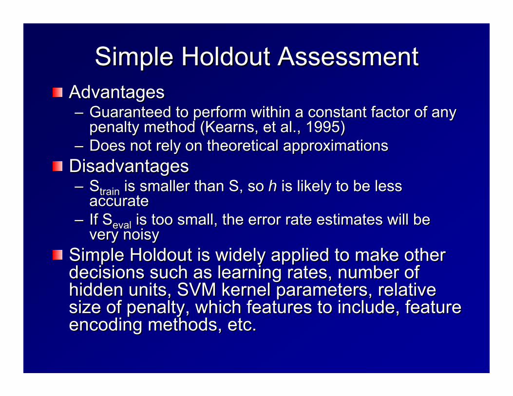
Simple Holdout AssessmentSimple Holdout AssessmentAdvantagesAdvantages–– Guaranteed to perform within a constant factor of any Guaranteed to perform within a constant factor of any

penalty method (Kearns, et al., 1995)penalty method (Kearns, et al., 1995)–– Does not rely on theoretical approximationsDoes not rely on theoretical approximations

DisadvantagesDisadvantages–– SStraintrain is smaller than S, so is smaller than S, so hh is likely to be less is likely to be less

accurateaccurate–– If SIf Sevaleval is too small, the error rate estimates will be is too small, the error rate estimates will be

very noisyvery noisySimple Holdout is widely applied to make other Simple Holdout is widely applied to make other decisions such as learning rates, number of decisions such as learning rates, number of hidden units, SVM kernel parameters, relative hidden units, SVM kernel parameters, relative size of penalty, which features to include, feature size of penalty, which features to include, feature encoding methods, etc.encoding methods, etc.

kk--fold Crossfold Cross--Validation to Validation to determine Hdetermine Hii

Randomly divide S into k equalRandomly divide S into k equal--sized subsetssized subsetsRun learning algorithm k times, each time use Run learning algorithm k times, each time use one subset for Sone subset for Sevaleval and the rest for Sand the rest for Straintrain

Average the resultsAverage the results

KK--fold Crossfold Cross--Validation to determine HValidation to determine Hii

Partition S into K disjoint subsets SPartition S into K disjoint subsets S11, S, S22, , ……, S, SkkRepeat simple holdout assessment K timesRepeat simple holdout assessment K times–– In the In the kk--th assessment, Sth assessment, Straintrain = S = S –– SSkk and Sand Sevaleval = S= Skk–– Let Let hhii

kk be the best hypothesis from Hbe the best hypothesis from Hii from iteration k.from iteration k.–– Let Let εεii be the average Sbe the average Sevaleval of of hhii

kk over the K iterationsover the K iterations–– Let iLet i** = argmin= argminii εεii

Train on S using HTrain on S using Hii** and output the resulting and output the resulting hypothesishypothesis

ii

55

44

33

22

11

kk

99887766554433221100

EnsemblesEnsemblesBayesian Model AveragingBayesian Model Averaging. Sample hypotheses . Sample hypotheses hhiiaccording to their posterior probability P(according to their posterior probability P(hh|S). Vote |S). Vote them. A method called Markov chain Monte Carlo them. A method called Markov chain Monte Carlo (MCMC) can do this (but it is quite expensive)(MCMC) can do this (but it is quite expensive)BaggingBagging. Overfitting is caused by high variance. . Overfitting is caused by high variance. Variance reduction methods such as bagging can help. Variance reduction methods such as bagging can help. Indeed, best results are often obtained by bagging Indeed, best results are often obtained by bagging overfitted classifiers (e.g., unpruned decision trees, overoverfitted classifiers (e.g., unpruned decision trees, over--trained neural networks) than by bagging welltrained neural networks) than by bagging well--fitted fitted classifiers (e.g., pruned trees).classifiers (e.g., pruned trees).Randomized CommitteesRandomized Committees. We can train several . We can train several hypotheses hypotheses hhii using different random starting weights for using different random starting weights for backpropagationbackpropagationRandom ForestsRandom Forests. Grow many decision trees and vote . Grow many decision trees and vote them. When growing each tree, randomly (at each them. When growing each tree, randomly (at each node) choose a subset of the available features (e.g., node) choose a subset of the available features (e.g., √√nnout of out of nn features). Compute the best split using only features). Compute the best split using only those features.those features.

Overfitting SummaryOverfitting SummaryMinimizing training set error (Minimizing training set error (εεtraintrain) does not necessarily ) does not necessarily minimize test set error (minimize test set error (εεtesttest).).–– This is true when the hypothesis space is too large (too This is true when the hypothesis space is too large (too

expressive)expressive)Penalty methods add a penalty to Penalty methods add a penalty to εεtraintrain to approximate to approximate εεtesttest–– Bayesian, MDL, and Structural Risk MinimizationBayesian, MDL, and Structural Risk Minimization

Holdout and CrossHoldout and Cross--Validation methods without a subset Validation methods without a subset of the training data, Sof the training data, Sevaleval, to determine the proper , to determine the proper hypothesis space Hhypothesis space Hii and its complexityand its complexityEnsemble Methods take a combination of several Ensemble Methods take a combination of several hypotheses, which tends to cancel out overfitting errorshypotheses, which tends to cancel out overfitting errors

Penalty Methods for decision trees, Penalty Methods for decision trees, neural networks, and SVMsneural networks, and SVMs

Decision TreesDecision Trees–– pessimistic pruningpessimistic pruning–– MDL pruningMDL pruningNeural NetworksNeural Networks–– weight decayweight decay–– weight eliminationweight elimination–– pruning methodspruning methodsSupport Vector MachinesSupport Vector Machines–– maximizing the marginmaximizing the margin

Pessimistic Pruning of Decision TreesPessimistic Pruning of Decision Trees

Error rate on training data is 4/20 = 0.20 = p.Error rate on training data is 4/20 = 0.20 = p.Binomial confidence interval (using the Binomial confidence interval (using the normal approximation to the binomial normal approximation to the binomial distribution) isdistribution) is

If we use If we use αα = 0.25, then z= 0.25, then zαα/2/2 = 1.150 so we = 1.150 so we obtainobtain

0.097141 0.097141 ·· p p ·· 0.3028590.302859

We use the upper bound of this as our error We use the upper bound of this as our error rate estimate. Hence, we estimate rate estimate. Hence, we estimate 0.302859 0.302859 ×× 20 = 6.06 errors20 = 6.06 errors

p−zα/2·sp(1− p)

n<= p <= p+zα/2·

sp(1− p)

n

Pruning Algorithm (1):Pruning Algorithm (1):Traversing the TreeTraversing the Tree

float Prune(Node & node)float Prune(Node & node){{if (node.leaf) return PessError(node);if (node.leaf) return PessError(node);float childError = Prune(node.left) + Prune(node.right);float childError = Prune(node.left) + Prune(node.right);float prunedError = PessError(node);float prunedError = PessError(node);if (prunedError < childError) { // pruneif (prunedError < childError) { // prunenode.leaf = true;node.leaf = true;node.left = node.right = NULL;node.left = node.right = NULL;return prunedError}return prunedError}

else // don't pruneelse // don't prunereturn childError;return childError;

}}

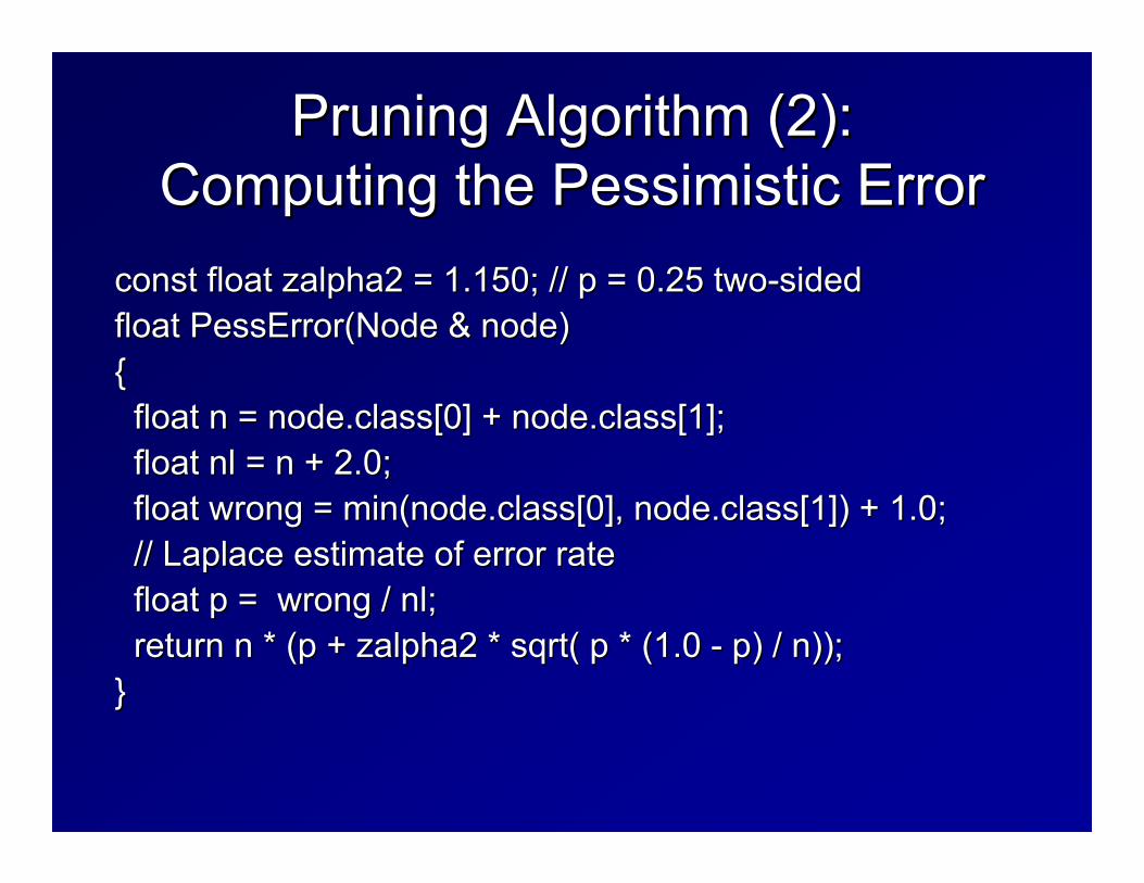
Pruning Algorithm (2):Pruning Algorithm (2):Computing the Pessimistic ErrorComputing the Pessimistic Error

const float zalpha2 = 1.150; // p = 0.25 twoconst float zalpha2 = 1.150; // p = 0.25 two--sidedsidedfloat PessError(Node & node)float PessError(Node & node){{float n = node.class[0] + node.class[1];float n = node.class[0] + node.class[1];float nl = n + 2.0;float nl = n + 2.0;float wrong = min(node.class[0], node.class[1]) + 1.0;float wrong = min(node.class[0], node.class[1]) + 1.0;// Laplace estimate of error rate// Laplace estimate of error ratefloat p = wrong / nl;float p = wrong / nl;return n * (p + zalpha2 * sqrt( p * (1.0 return n * (p + zalpha2 * sqrt( p * (1.0 -- p) / n));p) / n));

}}

Pessimistic Pruning ExamplePessimistic Pruning Example

Penalty methods for Neural Penalty methods for Neural NetworksNetworks

Weight DecayWeight Decay

Weight EliminationWeight Elimination

ww00 large encourages many small weightslarge encourages many small weightsww00 small encourages a few large weightssmall encourages a few large weights

Ji(W ) =1

2(yi− yi)2 + λ

Xj

w2j

Ji(W ) =1

2(yi− yi)2 + λ

Xj

w2j /w20

1+ w2j /w20

Weight EliminationWeight Elimination

This essentially counts the number of large weights. Once they This essentially counts the number of large weights. Once they are are large enough, their penalty does not changelarge enough, their penalty does not change

Neural Network Pruning Methods:Neural Network Pruning Methods:Optimal Brain DamageOptimal Brain Damage

(LeCun, Denker, Solla, 1990)(LeCun, Denker, Solla, 1990)

Taylor’s Series Expansionof the Squared Error:

∆J(W ) =Xj

gj∆wj+1

2

Xj

hjj(∆wj)2+1

2

Xj 6=k

hjk∆wj∆wk+O(||∆wj||3)

where

gj =∂J(W)

∂wjand hjk=

∂2J(W )

∂wj∂wk

At a local minimum, gj = 0.

Assume off-diagonal terms hjk = 0

∆J(W ) =1

2

Xj

hjj(∆wj)2

If we set wj = 0, the error will change by

hjjw2j /2

Optimal Brain Damage ProcedureOptimal Brain Damage Procedure

1.1. Choose a reasonable network architectureChoose a reasonable network architecture2.2. Train the network until a reasonable solution is Train the network until a reasonable solution is

obtainedobtained3.3. Compute the second derivatives hCompute the second derivatives hjjjj for each for each

weight wweight wjj

4.4. Compute the saliencies for each weight hCompute the saliencies for each weight hjjjjwwjj}}22/2/25.5. Sort the weights by saliency and delete some Sort the weights by saliency and delete some

lowlow--saliency weightssaliency weights6.6. Repeat from step 2Repeat from step 2

OBD ResultsOBD ResultsOn an OCR problem, they started with a highlyOn an OCR problem, they started with a highly--constrained and sparsely connected network constrained and sparsely connected network with 2,578 weights, trained on 9300 training with 2,578 weights, trained on 9300 training examples. They were able to delete more than examples. They were able to delete more than 1000 weights without hurting training or test 1000 weights without hurting training or test error.error.Optimal Brain Surgeon attempts to do this Optimal Brain Surgeon attempts to do this before reaching a local minimumbefore reaching a local minimumExperimental evidence is mixed about whether Experimental evidence is mixed about whether this reduced overfitting, but it does reduce the this reduced overfitting, but it does reduce the computational cost of using the neural networkcomputational cost of using the neural network

Penalty Methods for Support Vector Penalty Methods for Support Vector MachinesMachines

Our basic SVM tried to fit the training data perfectly Our basic SVM tried to fit the training data perfectly (possibly by using kernels). However, this will quickly (possibly by using kernels). However, this will quickly lead to overfitting.lead to overfitting.Recall marginRecall margin--based bound. With probability 1 based bound. With probability 1 –– δδ, a , a linear separator with unit weight vector and margin linear separator with unit weight vector and margin γγ on on training data lying in a ball of radius R will have an error training data lying in a ball of radius R will have an error rate on new data points bounded by rate on new data points bounded by

² <=C

m

"R2 + kξk2

γ2log2m+ log

1

δ

#

For some constant C. ξ is the margin slack vector such that

ξi =max{0, γ − yig(xi)}

Preventing SVM OverfittingPreventing SVM Overfitting

Maximize margin Maximize margin γγMinimize slack vector ||Minimize slack vector ||ξξ||||Minimize RMinimize R

The (reciprocal) of the margin acts as a The (reciprocal) of the margin acts as a penalty to prevent overfittingpenalty to prevent overfitting

Functional Margin versus Functional Margin versus Geometric MarginGeometric Margin

Functional margin: Functional margin: γγff = y= yii ·· ww ·· xxii

Geometric margin: Geometric margin: γγgg = = γγff/ ||/ ||ww||||

The margin bound applies only to the The margin bound applies only to the geometric margin geometric margin γγgg

The functional margin can be made The functional margin can be made arbitrarily large by rescaling the weight arbitrarily large by rescaling the weight vector, but the geometric margin is vector, but the geometric margin is invariant to scalinginvariant to scaling

Intermission: Geometry of LinesIntermission: Geometry of LinesConsider the line Consider the line ww ·· xx + b = 0, where ||+ b = 0, where ||ww|| = 1 is || = 1 is a vector of unit length. Then the minimum a vector of unit length. Then the minimum distance to the origin is b.distance to the origin is b.

Geometry of a MarginGeometry of a Margin

If a point If a point xx++ is a distance is a distance γγ away from the away from the line, then it lies on the line line, then it lies on the line ww ·· xx + b = + b = γγ

The Geometric Margin is the The Geometric Margin is the Inverse of ||Inverse of ||ww||||

Lemma: Lemma: γγgg = 1/||= 1/||ww||||Proof:Proof:–– Let Let ww be an arbitrary weight vector such that the be an arbitrary weight vector such that the

positive point positive point xx++ has a functional margin of 1. Thenhas a functional margin of 1. Thenww ·· xx++ + b = 1+ b = 1

–– Now normalize this equation by dividing by ||Now normalize this equation by dividing by ||ww||.||.

–– Implication: We can hold the functional margin at 1 Implication: We can hold the functional margin at 1 and minimize the norm of the weight vectorand minimize the norm of the weight vector

w

kwk · x++

b

kwk =1

kwk = γg

Support Vector Machine Quadratic Support Vector Machine Quadratic ProgramProgram

Find Find wwMinimize ||Minimize ||ww||||22

Subject toSubject toyyii ·· ((ww ·· xxii + b) + b) ≥≥ 11This requires every training example to This requires every training example to have a functional margin of at least 1 and have a functional margin of at least 1 and then maximizes the geometric margin. then maximizes the geometric margin. However it still requires perfectly fitting the However it still requires perfectly fitting the datadata

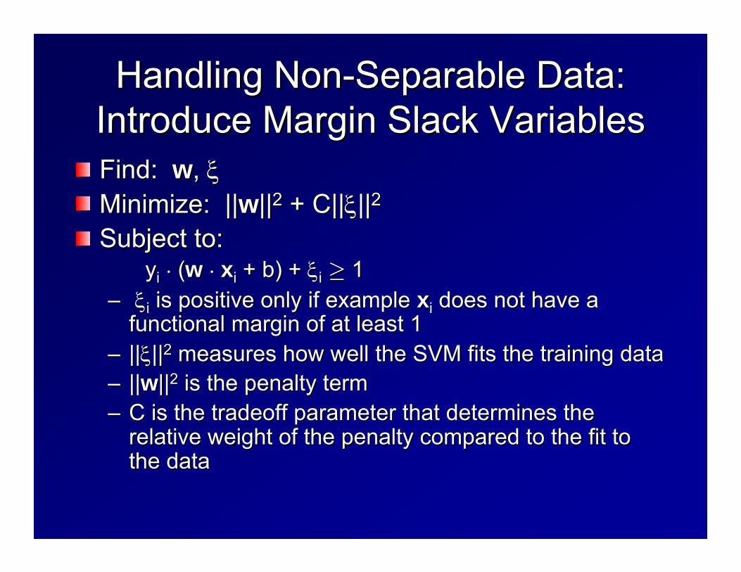
Handling NonHandling Non--Separable Data:Separable Data:Introduce Margin Slack VariablesIntroduce Margin Slack VariablesFind: Find: ww, , ξξMinimize: ||Minimize: ||ww||||22 + C||+ C||ξξ||||22Subject to:Subject to:

yyii ·· ((ww ·· xxii + b) + + b) + ξξii ≥≥ 11–– ξξii is positive only if example is positive only if example xxii does not have a does not have a

functional margin of at least 1functional margin of at least 1–– ||||ξξ||||22 measures how well the SVM fits the training datameasures how well the SVM fits the training data–– ||||ww||||22 is the penalty termis the penalty term–– C is the tradeoff parameter that determines the C is the tradeoff parameter that determines the

relative weight of the penalty compared to the fit to relative weight of the penalty compared to the fit to the datathe data

Kernel Trick Form of SVMKernel Trick Form of SVM

To apply the Kernel Trick, we need to To apply the Kernel Trick, we need to reformulate the SVM quadratic program so reformulate the SVM quadratic program so that it only involves dot products between that it only involves dot products between training examples. This can be done by training examples. This can be done by an operation called the Lagrange Dualan operation called the Lagrange Dual

Lagrange Dual ProblemLagrange Dual Problem

Find Find ααii

Minimize Minimize ∑∑ii ααii –– ½½ ∑∑ii ∑∑jj yyii yyjj ααii ααjj [[xxii ·· xxjj + + δδijij/C]/C]

Subject toSubject to∑∑ii yyii ααii = 0= 0ααii ≥≥ 00

where where δδijij = 1 if i = j and 0 otherwise.= 1 if i = j and 0 otherwise.

Kernel Trick FormKernel Trick Form

Find Find ααii

Minimize Minimize ∑∑ii ααii –– ½½ ∑∑ii ∑∑jj yyii yyjj ααii ααjj [K([K(xxii,,xxjj) + ) + δδijij/C]/C]

Subject toSubject to∑∑ii yyii ααii = 0= 0ααii ≥≥ 00

where where δδijij = 1 if i = j and 0 otherwise.= 1 if i = j and 0 otherwise.

Resulting ClassifierResulting Classifier

The resulting classifier isThe resulting classifier isf(f(xx) = ) = ∑∑jj yyjj ααjj K(K(xxjj, , xx) + b) + b

where b is chosen by finding an where b is chosen by finding an ii with with ααii > 0 and solving> 0 and solving

yyii f(f(xxii) = 1 ) = 1 –– ααii/C/Cfor f(for f(xxii))

Variations on the SVM Problem:Variations on the SVM Problem:Variation 1: Use LVariation 1: Use L11 norm of norm of ξξ

This is the This is the ““officialofficial”” SVM, which was SVM, which was originally published by Vapnik and Cortesoriginally published by Vapnik and CortesFind: Find: ww, , ξξMinimize: ||Minimize: ||ww||||22 + C||+ C||ξξ||||Subject to:Subject to:

yyii ·· ((ww ·· xxii + b) + + b) + ξξii ≥≥ 11

Dual Form of LDual Form of L11 SVMSVM

Find Find ααii

Minimize Minimize ∑∑ii ααii –– ½½ ∑∑ii ∑∑jj yyii yyjj ααii ααjj K(K(xxii,,xxjj))

Subject toSubject to∑∑ii yyii ααii = 0= 0C C ≥≥ ααii ≥≥ 00

Variation 2: Variation 2: Linear Programming SVMsLinear Programming SVMs

Use LUse L11 norm for norm for ww tootooFind Find uu, , vv, , ξξMinimize Minimize ∑∑jj uujj + + ∑∑jj vvjj + C + C ∑∑ii ξξiiSubject toSubject to

yyii ·· ((((uu –– vv) ) ·· xxii + b) + + b) + ξξii ≥≥ 11The kernel form of this isThe kernel form of this isFind Find ααii, , ξξMinimize Minimize ∑∑ii ααii + C + C ∑∑ii ξξiiSubject toSubject to

∑∑jj ααjj yyii yyjj K(K(xxii,,xxjj) + ) + ξξii ≥≥ 11ααjj ≥≥ 00

Setting the Value of CSetting the Value of CWe see that the full SVM algorithm requires We see that the full SVM algorithm requires choosing the value of C, which controls the choosing the value of C, which controls the tradeoff between fitting the data and obtaining a tradeoff between fitting the data and obtaining a large margin.large margin.To set C, we could train an SVM with different To set C, we could train an SVM with different values of C and plug the resulting C, values of C and plug the resulting C, γγ, and , and ξξinto the margin bounds theorem to choose the C into the margin bounds theorem to choose the C that minimizes the bound on that minimizes the bound on εε..In practice, this does not work well, and we must In practice, this does not work well, and we must rely on holdout methods (next lecture).rely on holdout methods (next lecture).