City University of New York (CUNY) City University of New York (CUNY)

CUNY Academic Works CUNY Academic Works

Publications and Research City College of New York

2018

The price of a vote: Diseconomy in proportional elections The price of a vote: Diseconomy in proportional elections

Hygor Piaget M. Melo Instituto Federal de Educacao

Saulo D. S. Reis Universidade Federal do Ceara

Andre A. Moreira Universidade Federal do Ceara

Hernan Makse CUNY City College of New York

Jose S. Andrade Jr. Universidade Federal do Ceara

How does access to this work benefit you? Let us know!

More information about this work at: https://academicworks.cuny.edu/cc_pubs/701

Discover additional works at: https://academicworks.cuny.edu

This work is made publicly available by the City University of New York (CUNY). Contact: AcademicWorks@cuny.edu

RESEARCH ARTICLE

The price of a vote: Diseconomy in

proportional elections

Hygor Piaget M. Melo1,2*, Saulo D. S. Reis2, Andre A. Moreira2, Hernan A. Makse2,3, Jose

S. Andrade Jr.2

1 Instituto Federal de Educacão, Ciência e Tecnologia do Ceara, Avenida Des. Armando de Sales Louzada,

Acarau, Ceara, Brazil, 2 Departamento de Fısica, Universidade Federal do Ceara, 60451-970 Fortaleza,

Ceara, Brazil, 3 Levich Institute and Physics Department, City College of New York, New York, NY 10031,

United States of America

* hygor.piaget@ifce.edu.br

Abstract

The increasing cost of electoral campaigns raises the need for effective campaign planning

and a precise understanding of the return of such investment. Interestingly, despite the

strong impact of elections on our daily lives, how this investment is translated into votes is

still unknown. By performing data analysis and modeling, we show that top candidates

spend more money per vote than the less successful and poorer candidates, a relation that

discloses a diseconomy of scale. We demonstrate that such electoral diseconomy arises

from the competition between candidates due to inefficient campaign expenditure. Our

approach succeeds in two important tests. First, it reveals that the statistical pattern in the

vote distribution of candidates can be explained in terms of the independently conceived,

but similarly skewed distribution of money campaign. Second, using a heuristic argument,

we are able to explain the observed turnout percentage for a given election of approximately

63% in average. This result is in good agreement with the average turnout rate obtained

from real data. Due to its generality, we expect that our approach can be applied to a wide

range of problems concerning the adoption process in marketing campaigns.

Introduction

Elections exhibit a complex process of negotiations between politicians and voters. The past

few decades bore witness to a steep increase in the expenditure of political campaigns. Take

the example of the presidential elections in the US. The 1996 campaigns cost contestants

approximately $123 million (corrected for inflation) altogether, an amount that escalated to

nearly $2 billion in 2012 [1]. Although campaign investments have grown, the impact of

money on the electoral outcome remains not fully understood [2–4], and conclusions about it

are quite contradictory. In some studies, it has been argued that incumbent spending is inef-

fective, and the challenger spending, on the other hand, produces large gains [5–7]. Other

studies claim that neither incumbent nor challenger spending makes any appreciable differ-

ence [8, 9], a theory that dates back to the 1940’s [10, 11]. Yet another group argues that both

challenger and incumbent spending are effective [12].

PLOS ONE | https://doi.org/10.1371/journal.pone.0201654 August 22, 2018 1 / 13

a1111111111

a1111111111

a1111111111

a1111111111

a1111111111

OPENACCESS

Citation: Melo HPM, Reis SDS, Moreira AA, Makse

HA, Andrade JS, Jr. (2018) The price of a vote:

Diseconomy in proportional elections. PLoS ONE

13(8): e0201654. https://doi.org/10.1371/journal.

pone.0201654

Editor: Michael Szell, Central European University,

HUNGARY

Received: March 4, 2018

Accepted: July 19, 2018

Published: August 22, 2018

Copyright: © 2018 Melo et al. This is an open

access article distributed under the terms of the

Creative Commons Attribution License, which

permits unrestricted use, distribution, and

reproduction in any medium, provided the original

author and source are credited.

Data Availability Statement: All files are publicly

available at the http://www.tse.gov.br/.

Funding: HPMM, SDSR, AAM, HAM and JSA were

supported by Conselho Nacional de

Desenvolvimento Cientıfico e Tecnologico (CNPq),

Coordenacão de Aperfeicoamento de Pessoal de

Nıvel Superior (CAPES), Fundacão Cearense de

Apoio ao Desenvolvimento Cientıfico e Tecnologico

(FUNCAP), National Institute of Science and

Technology for Complex Systems (INCT-SC), and

Army Research Laboratory Cooperative Agreement

Despite the questioning about the effectiveness of political campaigns as a whole, the elec-

tion campaign of President Barack Obama in 2012 spent more than 65% of its money on

media, including TV and radio air time, digital and printing advertising, and others [13].

Therefore, the direct contact with voters is not only a major factor in campaign planning, but

it is believed to have relevant impact in succeeding to persuade undecided voters [14].

Here we address the problem of how campaign expenditure influences election outcome.

We start by an extensive analysis of data sets from the proportional elections in Brazilian states

for the federal and state congresses, uncovering a ubiquitous nonlinearity on the relation

between votes and campaign budget. As we will show, candidates can be gathered into differ-

ent groups of spenders. One group is characterized by candidates with low budget campaign

and a seemingly uncorrelated number of votes. As the money invested on campaign increases,

a clear correlation between vote and money emerges. Interestingly, in this correlated regime,

the top candidates are those who spend more in political campaign, but with a highly counter-

intuitive result: the more the candidates spend, the less vote per dollar they get.

In Economics, a similar effect in which larger companies tend to produce goods at

increased per-unit costs is known as diseconomy of scale. Precisely, the diseconomy of scale

makes reference to a financial drawback resulting from the increase of the production scale. In

the cases where a diseconomy of scale is verified, above a maximum efficient company size,

the average cost per unit production increases. In other words, above this maximum, the more

companies invest to increase in size, the less return of such investments they get per produced

unit. The origin of this type of behavior can be manifold. For instance, it has been explained in

terms of a systematic increase in communication costs [15], or as a consequence of the Ringel-

mann psychological effect, namely, the tendency for individuals to become less efficient when

working in larger groups [16]. To the best of our knowledge, this study is the first to report the

presence of diseconomy of scale on elections.

In order to elucidate the mechanisms responsible for this diseconomy in elections, we

develop a general model for the negotiations between candidates and voters whose solution is

compared with results from the analysis of electoral data sets. An important assumption in our

model is that votes are considered to be “buyable”, whether they are somehow purchased

through direct contacts between candidates and voters or, indirectly, through media cam-

paigns. In this way, since the amount of financial resources mi effectively represents the main

convincing strength of candidate i, it also provides an upper bound for the number of votes

that can be received, when competition among candidates is regarded as absent. The potential

ability of a candidate to acquire votes in this model can be estimated, as a first approximation,

in terms of the identification of the influential spreaders [17, 18].

A crucial goal here is to show that the competition between candidates is the root cause of

the diseconomy of scale observed in Brazilian elections, mainly due to the fact that, in a sce-

nario without competition, any model prediction will have a tendency to overestimate the

number of votes of top campaign spenders. Our results show that the introduction of competi-

tion among candidates in the model combined with a simple heuristic argument lead to a pre-

diction for the turnout rate of elections that is compatible with the average value from real

data. We obtain this by the assumption that campaign planners would make use of financial

resources considering an equitable division of funds per vote.

A direction not explored in this work is the explanation of the relation between money and

votes where campaign funding is correlated with the vote share received in the previous elec-

tion. However, the non-linearity can also be seen as indication of potential causal relationship

in the direction of votes as a consequence of campaign funding. Important to note, in Brazil

parties receive money campaign in proportion to the current number of deputies in the cham-

ber, but the parties are free to choose an uneven distribution of funding among the candidates.

The price of a vote

PLOS ONE | https://doi.org/10.1371/journal.pone.0201654 August 22, 2018 2 / 13

Number W911NF-09-2-0053 (the ARL Network

Science CTA).

Competing interests: The authors have declared

that no competing interests exist.

Results

Empirical findings

Our data analysis is based on real data sets acquired from recent proportional elections in

Brazil, publicly available [19]. These data sets are related to the elections for the national

lower house and state congress in 2014. Brazilian elections represent a quite general and suit-

able case study to our purposes due to a number of special factors. First, Brazil is a large

country, both in population and land area. It has the fifth largest population of the world

spread across roughly 8.5 million km2 (over 3 million mi2). Second, in contrast with execu-

tive elections, representative elections in Brazil have a large number of candidates. Addition-

ally, it is compulsory to vote in Brazil. Altogether, these factors lead to a huge data set from a

quite diverse electorate.

We start by assembling the data sets on the entire electoral outcome and campaign expendi-

ture of candidates from all 26 Brazilian states. Fig 1 displays the number of votes v versus the

declared campaign expenditure m of each candidate for the top 4 Brazilian states in terms of

population, namely, São Paulo (Fig 1A and 1B), Rio de Janeiro (Fig 1C and 1D), Minas Gerais

(Fig 1E and 1F) and Bahia (Fig 1G and 1H). As depicted in Fig 1, the clouds of points are neatly

correlated and follow a clear trend. This trend is observed in all representative elections for all

Brazilian states (see Supporting Information Section I).

To extract the main relationship between v and m, we average the number of votes in log-

spaced bins along m, which provides an estimation for the empirical relation of v as a function

of m. In order to plot results for different states in the same figure, we perform a scale transfor-

mation on v by supposing simple linear relation v = c ×m, where c is a characteristic constant

of a given election. If we define the average price of a vote as Δm = ∑i mi/∑i vi and suppose that

it is roughly uniform across candidates, it is easy to see that c = 1/Δm. Here, vi is the number of

votes of candidates i. If the relation between votes and money is linear, then the plot of v ×(Δm/m) should be a constant function of m with value close to 1.0.

In Fig 1I and 1J, we plot vΔm/m as a function of m for the state legislative assembly and fed-

eral congress elections, respectively, for the year of 2014 and for the eight most populated states

in Brazil. The result shows a consistent nontrivial dependence of votes on money spent in cam-

paign. For small values of m, we observe a rapidly decrease of vΔm/m. For intermediate expen-

ditures in the range R$10,000<m< R$100,000, we observe an apparent linear dependence of vwith respect to m (at election day, October 5th, 2014, the exchange rate between the Dollar and

the Brazilian Real was R$ 2.4266 = $1). Finally, for m> R$100,000, a noticeable departure

from linearity is observed, that is, wealthier candidates need a disproportionately large amount

of money to obtain a single vote as compared with less successful candidates within the same

range of financial resources.

A general model for the price of a vote

Here, we propose a general model for the price of a vote. We consider an electoral process

composed of two separate groups of individuals, candidates and voters. All s candidates can

compete for the vote of all n voters, and each candidate i has a limited amount of money mi to

spend on their campaigns. Thus, if at a given time mi = 0, the candidate becomes unable to

compete for voters anymore. Here we assume that candidates can only conquer a single vote at

a given time step and that voters, once they reach a decision, cannot change their minds any-

more. As compared to the case of plurality elections, the last assumption is readily justifiable

for proportional elections since, in this case, candidates do not compete directly for the same

seat. As a consequence, voters do not feel compelled to rethink their decisions. In this way,

The price of a vote

PLOS ONE | https://doi.org/10.1371/journal.pone.0201654 August 22, 2018 3 / 13

Fig 1. Scaling relation between number of votes and money spent. The light purple circles show the relation between the number of votes and the

declared campaign expenditure of each candidate in the state (SD) and federal deputies (FD) elections in 2014 for the four largest states in Brazil: São

Paulo (A, B), Rio de Janeiro (C, D), Minas Gerais (E, F), and Bahia (G, H). Despite the large fluctuations, there is an unambiguous correlation

between votes and money. In each panel, the data for elected candidates are highlighted in dark purple circles. In order to see the nuances of the

The price of a vote

PLOS ONE | https://doi.org/10.1371/journal.pone.0201654 August 22, 2018 4 / 13

because it is not possible to know if a voter reached a decision or not, campaigns can spend

money on already decided voters, leading to ineffective use of financial resources.

A pictorial description of the model is presented in Fig 2. On a social network with unde-

cided voters, represented by light gray individuals, two candidates start their campaigns with

an initial amount of money m and one single decided voter. This initial seed is represented in

Fig 2A by the blue and red individuals. The regions highlighted in blue and red represent the

operational areas of the campaigns, enclosing the group of voters to whom the campaigns will

spend money in order to turn undecided voters into decided voters. As depicted in Fig 2B, at

each time step each campaign chooses one voter inside its operational areas. If the chosen indi-

vidual is an undecided voter, she/he becomes a decided voter. Accordingly, the overall cam-

paign money is decreased by an amount of Δm. If the chosen voter is already a decided voter,

as depicted in Fig 2C, the campaign budget is also decreased by Δm, but the voter’s decision

remains unchanged. We repeat this procedure until all campaigns run out of funds. In Fig 2D,

we show a typical example of a competition for votes between two candidates during the elec-

toral process described by our model. Although the candidate with the larger initial budget

receives more votes at the end of the election, due to ineffective spending, the campaign of the

poorer candidate is, in fact, more efficient.

In order to represent the reach of the traditional and social medias, as a first approximation,

we apply this model on a complete graph, so that the time evolution of the number of votes of

a given candidate i can be written as

dvi

dt¼ 1 �

SðtÞn

� �

½miðtÞ > 0�; ð1Þ

where SðtÞ ¼Ps

i¼0vi is the total number of decided voters at time t, and [mi(t)> 0] is the Iver-

son bracket, which is 1 if the condition inside the brackets is satisfied, and 0 otherwise. The

right-hand side of the Eq 1 is the probability of candidate i to choose an undecided voter at

time t. Eq 1 explicitly requires a definition for the rate of money expenditure, dmi/dt, which

determines the gradual decrease in financial resources of candidate i. As simplifying assump-

tions, we consider that the amount of money spent during the campaign decreases linearly,

dmi/dt = −Δmi, and that this constant rate is the same for all candidates, Δmi = Δm, 8i.The probabilistic feature of Eq 1 is central to confirm our hypothesis that electoral outcome

is an output of campaign expenditure due to a competition process. This is shown here by first

considering the case without competition, where S� n. Also, we assume that nΔm� mi for

all i, so that the candidate with the highest amount of funds does not have enough money to

reach out the whole network. By doing so, it is unlikely that the extent of the candidates’ cam-

paigns overlap, and therefore, a candidate would not waste her/his campaign money on a

decided voter of another candidate. As a consequence, since the probability of candidate i to

conquer an undecided voter is not affected by another campaign, S(t) can be replaced by vi in

Eq 1, leading to an uncoupled system of differential equations, whose solution is given by,

vi ¼ n � ðn � v0;iÞe� mi=nDm; ð2Þ

where v0,i is the initial number of votes of candidate i. Since nΔm� mi, and assuming that

(n − v0,i)� n, by expanding the exponential and taking its first order approximation, we can

correlation, we plotted in a normalized relation for (I) state and (J) federal deputies for the eight largest states in Brazil. The symbols represent the

normalized ratio hviΔm/m, where we first calculate the average number of votes in log-spaced bins along m. If we assume a linear correlation, the

multiplicative constant is Δm = M/n. The normalization provides us a direct observation of the nonlinearity in the dependence of votes on money.

We see a global sublinear behavior, where the wealthier candidates display a lower fraction of votes per money.

https://doi.org/10.1371/journal.pone.0201654.g001

The price of a vote

PLOS ONE | https://doi.org/10.1371/journal.pone.0201654 August 22, 2018 5 / 13

write the number of votes as vi� v0,i + mi/Δm. As we discuss next, this simple model does not

suffice to explain the whole complexity of the relation between v and m. The first two regimes

presented in Fig 1 can be understood in terms of this approximation. For the regime of low m,

where the experimental data do not exhibit a clear correlation, the candidates start the race

with v0,i votes. Since they cannot afford a long run and/or a large expenditure, their final per-

formance fluctuates around the initial value v0,i, which depends on different factors, such as

free volunteer engagement. As campaign money increases, the linear part overcomes the initial

number v0,i, and a linear regime emerges. However, in the scenario without competition, the

linear behavior remains at large m.

We now consider the competition between candidates as a possible cause for the transition

from linear to sublinear regime. Disregarding all previous simplifying assumptions and inte-

grating Eq 1, we find

vi ¼ v0;i þmi

Dm�

1

nDm

Z mi

0

Sðm0Þdm0; ð3Þ

where the integration of the Iverson bracket over time gives the total time candidate i has to

perform her/his campaign, mi/Δm, and we used dm0/dt0 = −Δm to change the variable of inte-

gration on the last term.

It is possible to find a differential equation for S(m0) by taking Eq 1 and summing over i.After solving it for S(m0) and integrating the last term of Eq 3 (see Supporting Information Sec-

tion II for details of the analytical solution), we find a set of nonlinear coupled equations that

must be solved, candidate by candidate, following an increasing order of mi values. As a conse-

quence, the number of votes of candidate i depends on the whole distribution P(m) through

the integral term in Eq 3.

Eq 3 has a simple interpretation. As in the case without competition, all candidates begin

their run with an initial number of votes, and those with sufficient money to keep running

enter in a linear regime controlled by the rate Δm/m. Nonetheless, as we will see next,

Fig 2. Model’s pictorial sketch. Here, two candidates compete for votes in a social network with undecided (light gray) individuals. (A) The blue candidate has initially a

budget of 4 (four) monetary units, while the campaign for the red candidate has a budget of 2 (two) monetary units. In this example, both candidates also have one

decided voter at the beginning of the process, namely, the blue voter at the top part of the network and the red one at the bottom part of the network. The highlighted

regions enclose the initial voter each campaign has and the acquaintances of each initial voter. These regions represent operational areas the campaigns will act at the next

time step in order to convince undecided voters to vote for their associated candidates. (B) One undecided voter inside each operational area is randomly chosen,

becoming then decided voters. Accordingly, each budget campaign decreases by the amount of Δm = $. As a consequence of new decided voters, the operational areas

grow, and since two acquaintances become voters of different candidates, the operational areas of the campaigns now overlap. This region where both campaigns can act

is represented in yellow. (C) While the red candidate’s campaign chose an undecided voter, increasing its operational area, blue campaign ineffectively spends money on

a decided voter. (D) At the end of the campaign process, when all campaigns run out of funds, the campaign with larger initial budget ends the process with more

adopters, but his/her campaign is less efficient, resulting in a diseconomy of scale.

https://doi.org/10.1371/journal.pone.0201654.g002

The price of a vote

PLOS ONE | https://doi.org/10.1371/journal.pone.0201654 August 22, 2018 6 / 13

candidates with sufficient campaign funds may start to waste their money on decided voters, a

behavior that is substantiated by the presence of S(m0) in the last term of Eq 3, which encloses

the competition dynamics. We consider this collective influence of the total financial resources

from all candidates during the campaign as an important result, since it provides a bridge

between campaign expenditure and electoral outcome, which is the basis of the remaining

results that follow.

In order to obtain a solution for the model, we use as inputs the money mi of each candidate

i, obtained from data, the total number of voters n, an initial number of votes v0, and an esti-

mated value for Δm. As a simplification, we assume that all candidates starts in average with

the same number of votes, v0 = v0,i. We define v0 as the average number of votes of candidates

with less than R$1,000. This assumption is a consequence of the low correlation between votes

and money when m< 1000. Therefore, we can better extract the value of v0 without a strong

influence of m. Note that one can choose a homogeneous distribution for v0,i without lack of

generality. As depicted in Fig 1I and 1J, for m< R$1, 000, the quantity hviΔm/m decays line-

arly, meaning that v is constant in average in this region. From this perspective, according to

Eq (3), one can consider that the candidates start the competition for votes with an initial v0 in

average, and receive more votes depending on their individual resources mi. The parameter

Δm is calculated as a function of the turnout rate T = Sf/n, where Sf = limt!1 S(t) is the total

number of votes at steady state. We can therefore write the final fraction of votes as

T ¼ 1 � e� M=ðnDmÞ; ð4Þ

where M = ∑i mi is the total amount of money in the campaign process. Therefore, we estimate

Δm using Eq 4 such that the total number of votes fits the turnout election data.

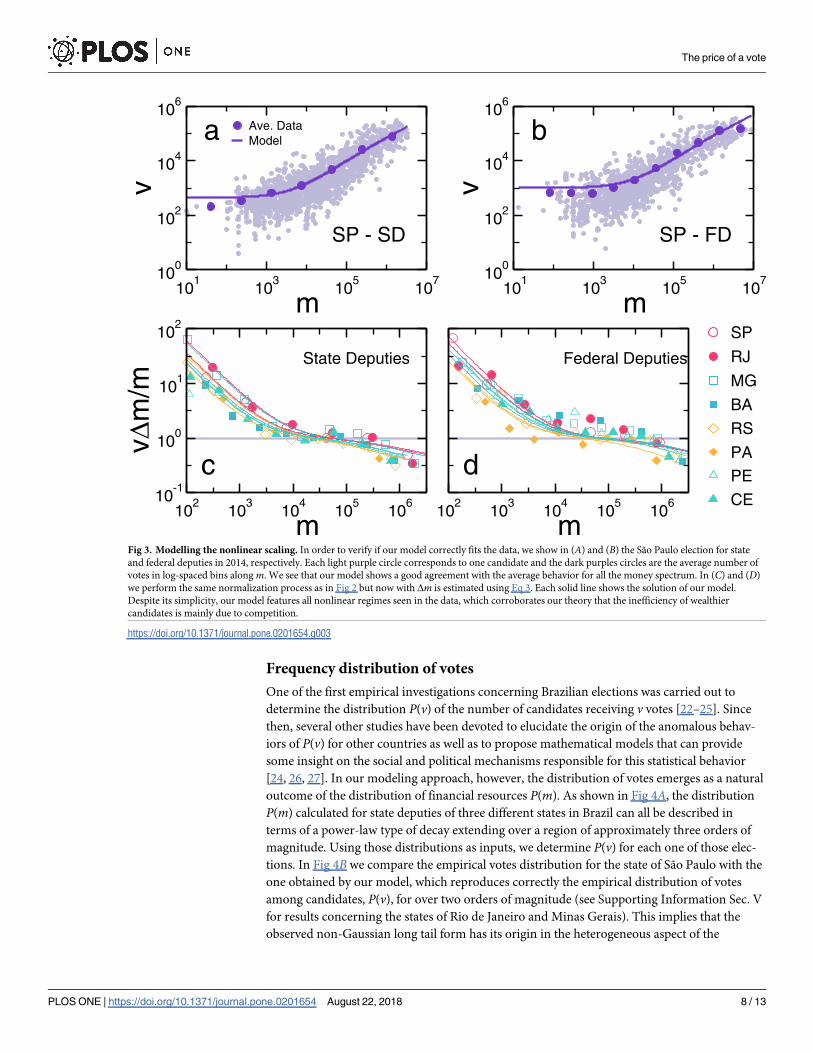
The results of the election in São Paulo state for state and federal deputies in 2014 are

shown in Fig 3A and 3B, respectively. As depicted, the predictions of our model (solid line) are

in good agreement with the average values of the number of votes for different classes of candi-

dates in terms of fund raising. Note that we only have two parameters, namely, Δm and v0.

Although they have an intuitive interpretation in the context of the model, only Δm has an

impact for large values of m. For m< R$1,000, our model exhibits a constant behavior, captur-

ing the uncorrelated nature of the data. Additionally, for m> R$1,000, an evident correlation

between votes and money is present. This is better visualized when we plot in Fig 3C and 3Dthe normalized ratio hviΔm/m for the eight most populated Brazilian states. Here, the symbols

represent the data average and the lines show the solution of our model for each state identi-

fied by color. For small and large values of m, we see that our model exhibits a clear deviation

from a linear behavior. In other words, besides exhibiting this deviation for m< R$1,000, a

clear sublinearity is present for m> R$100,000. Under the perspective of our model, the

observed diseconomy of scale is a direct consequence of the competition among candidates

(see Supporting Information Section III for a statistical comparison between our model with

competition and the linear model without competition).

Social networks are known to display the small-world phenomenon, where the typical net-

work distance between two individuals, ℓ, is rather small when compared to the system size,

ℓ * log N [20, 21]. Our analytical solution on a complete graph works as a first approximation

of such complex social network structure. In order to verify the validity of our solution, we

apply the dynamics presented on Fig 2 on random graphs of different average degree hki [21]

(see Supporting Information Section IV). We found a good agreement between the solution

on a complete graph model and the numerical simulation results obtained with a random

graph model.

The price of a vote

PLOS ONE | https://doi.org/10.1371/journal.pone.0201654 August 22, 2018 7 / 13

Frequency distribution of votes

One of the first empirical investigations concerning Brazilian elections was carried out to

determine the distribution P(v) of the number of candidates receiving v votes [22–25]. Since

then, several other studies have been devoted to elucidate the origin of the anomalous behav-

iors of P(v) for other countries as well as to propose mathematical models that can provide

some insight on the social and political mechanisms responsible for this statistical behavior

[24, 26, 27]. In our modeling approach, however, the distribution of votes emerges as a natural

outcome of the distribution of financial resources P(m). As shown in Fig 4A, the distribution

P(m) calculated for state deputies of three different states in Brazil can all be described in

terms of a power-law type of decay extending over a region of approximately three orders of

magnitude. Using those distributions as inputs, we determine P(v) for each one of those elec-

tions. In Fig 4B we compare the empirical votes distribution for the state of São Paulo with the

one obtained by our model, which reproduces correctly the empirical distribution of votes

among candidates, P(v), for over two orders of magnitude (see Supporting Information Sec. V

for results concerning the states of Rio de Janeiro and Minas Gerais). This implies that the

observed non-Gaussian long tail form has its origin in the heterogeneous aspect of the

Fig 3. Modelling the nonlinear scaling. In order to verify if our model correctly fits the data, we show in (A) and (B) the São Paulo election for state

and federal deputies in 2014, respectively. Each light purple circle corresponds to one candidate and the dark purples circles are the average number of

votes in log-spaced bins along m. We see that our model shows a good agreement with the average behavior for all the money spectrum. In (C) and (D)

we perform the same normalization process as in Fig 2 but now with Δm is estimated using Eq 3. Each solid line shows the solution of our model.

Despite its simplicity, our model features all nonlinear regimes seen in the data, which corroborates our theory that the inefficiency of wealthier

candidates is mainly due to competition.

https://doi.org/10.1371/journal.pone.0201654.g003

The price of a vote

PLOS ONE | https://doi.org/10.1371/journal.pone.0201654 August 22, 2018 8 / 13

distribution of campaign resources, regardless of the intricate social network and information

dynamics behind the electoral process.

Model validation

To highlight the effect of the sublinearity on forecasting an election, we compute the relative

difference between the cumulative vote distribution predicted by the linear model without

competition and the one predicted by the model with competition. As shown in Fig 4C, for

state congress election in the top three populated Brazilian states, namely, São Paulo, Rio de

Janeiro, and Minas Gerais, no significant difference is noticed between the two predictions for

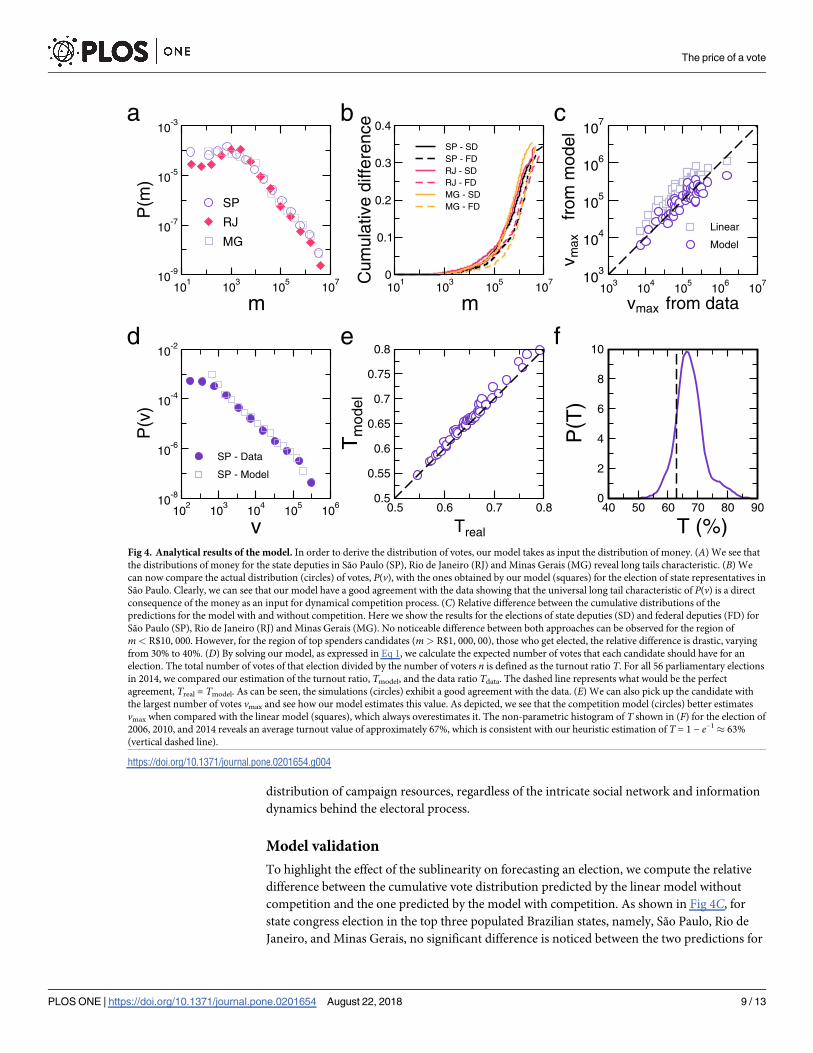
Fig 4. Analytical results of the model. In order to derive the distribution of votes, our model takes as input the distribution of money. (A) We see that

the distributions of money for the state deputies in São Paulo (SP), Rio de Janeiro (RJ) and Minas Gerais (MG) reveal long tails characteristic. (B) We

can now compare the actual distribution (circles) of votes, P(v), with the ones obtained by our model (squares) for the election of state representatives in

São Paulo. Clearly, we can see that our model have a good agreement with the data showing that the universal long tail characteristic of P(v) is a direct

consequence of the money as an input for dynamical competition process. (C) Relative difference between the cumulative distributions of the

predictions for the model with and without competition. Here we show the results for the elections of state deputies (SD) and federal deputies (FD) for

São Paulo (SP), Rio de Janeiro (RJ) and Minas Gerais (MG). No noticeable difference between both approaches can be observed for the region of

m< R$10, 000. However, for the region of top spenders candidates (m> R$1, 000, 00), those who get elected, the relative difference is drastic, varying

from 30% to 40%. (D) By solving our model, as expressed in Eq 1, we calculate the expected number of votes that each candidate should have for an

election. The total number of votes of that election divided by the number of voters n is defined as the turnout ratio T. For all 56 parliamentary elections

in 2014, we compared our estimation of the turnout ratio, Tmodel, and the data ratio Tdata. The dashed line represents what would be the perfect

agreement, Treal = Tmodel. As can be seen, the simulations (circles) exhibit a good agreement with the data. (E) We can also pick up the candidate with

the largest number of votes vmax and see how our model estimates this value. As depicted, we see that the competition model (circles) better estimates

vmax when compared with the linear model (squares), which always overestimates it. The non-parametric histogram of T shown in (F) for the election of

2006, 2010, and 2014 reveals an average turnout value of approximately 67%, which is consistent with our heuristic estimation of T = 1 − e−1� 63%

(vertical dashed line).

https://doi.org/10.1371/journal.pone.0201654.g004

The price of a vote

PLOS ONE | https://doi.org/10.1371/journal.pone.0201654 August 22, 2018 9 / 13

campaigns of low expenditure. However, for electoral campaigns that invested more than

R$10, 000, a substantial discrepancy between predictions can be noticed. For this region of top

spenders, the cumulative difference can be drastic, going above 30% in some cases.

We confirm the validity of our model by comparison with data from the 2014 state and fed-

eral deputy elections that took place simultaneously in the 26 states of Brazil. As shown in Fig

4D, where each point corresponds to an election in a given state, the model results for the turn-

out rate T, as provided by Eq 4, are compatible with the observed data. This agreement only

confirms the self-consistency of our approach, since Eq 3 has been used to estimate the param-

eter Δm. The predictive capability of the model can be effectively tested by comparing its esti-

mate with real data for the largest number of votes obtained by a candidate in each election,

vmax. As shown in Fig 4E, while the results of our model (circles) gather around the identity

line, demonstrating good quantitative agreement with real data, the linear approximation

model, vmax� v0+ mmax/Δm (squares), clearly overestimates the values of vmax.

At this point, we show that our theoretical framework can provide us an estimate for the

turnout ratio T in Brazilian proportional elections, if the following assumptions are consid-

ered: (i) the candidates have knowledge of the total amount of resources M during the cam-

paign, and (ii) Δm = M/n, which corresponds to the most simple and equitable division of

votes. As matter of fact, this last point is equivalent to assume that a complete turnout can be

achieved, namely, T = 100%, as in the case without competition. In other words, the candidates

devise their strategy presupposing that they will obtain the maximum possible number of

votes, therefore disregarding the competition among them. This heuristic argument leads to a

fraction of valid votes, T = 1 − e−1� 0.63. As shown in Fig 4F, the histogram of the number of

total valid votes for all Congress elections in the years 2006, 2010 and 2014 indicates an average

turnout value of 0.67, which is in close agreement with our model prediction. Finally, we also

tested our theoretical approach by applying the principle of maximum entropy [28] and found

that the statistical dispersion of the model is consistent with real data from elections (see Sup-

porting Information Sec. VI).

Discussion

As a result of the competition between candidates in real elections, the nonlinear relation

between v and m obtained here can complement other statistical analyses for political cam-

paign and electoral outcome [29–34]. These analyses enable the detection of a number of sta-

tistical patterns of electoral processes, such as the relations between party size and temporal

correlations [35], the relations between the number of candidates and voters [36], and the dis-

tribution of votes [22, 26, 27, 37]. Our approach goes beyond the examination of statistical pat-

terns by providing a theoretical framework that clarifies a number of key issues on the

economic features of electoral campaigns. First, we proposed a simple modeling framework,

whose analytical solution is statistically consistent with extensive data relating financial

resources of political and electoral outcomes. Interestingly, the same model also provides esti-

mates for the distribution of votes among candidates and the electorate turnout rate that are in

good agreement with real data.

A close inspection of the campaign data investigated here reveals a ubiquitous nontrivial

relation between v and m for all elections investigated. More precisely, we observed that this

relation is an unambiguous sublinear correlation between the money spent by candidate and

her/his number of votes v, specially for the top spender candidates, indicating that the electoral

process works in a state of diseconomy of scale. To explain this behavior in the campaign econ-

omy, we propose a general model for marketing where candidates compete with each other

and must spend their money in order to get votes. Despite its simplicity, the model proves

The price of a vote

PLOS ONE | https://doi.org/10.1371/journal.pone.0201654 August 22, 2018 10 / 13

capable of reproducing the complexity of the dependence of v with respect of m. This good

agreement makes our model a possible alternative to study other aspects of human collective

behavior involving, for example, diffusion of innovation and decision-making, such as the

competition in market share where companies invest in advertising for products.

Supporting information

S1 File. Supporting information file. In the S1 File (PDF) we present further details about the

data, statistical test, and the analytical derivation.

(PDF)

Acknowledgments

We thank the Brazilian agencies CNPq, CAPES, FUNCAP, and the National Institute of Sci-

ence and Technology for Complex Systems (INCT-SC) in Brazil for financial support, and the

support by Army Research Laboratory Cooperative Agreement Number W911NF-09-2-0053

(the ARL Network Science CTA) in the US.

Author Contributions

Conceptualization: Hygor Piaget M. Melo, Jose S. Andrade, Jr.

Data curation: Hygor Piaget M. Melo.

Formal analysis: Hygor Piaget M. Melo, Saulo D. S. Reis, Jose S. Andrade, Jr.

Funding acquisition: Jose S. Andrade, Jr.

Investigation: Hygor Piaget M. Melo, Saulo D. S. Reis, Andre A. Moreira, Hernan A. Makse,

Jose S. Andrade, Jr.

Methodology: Hygor Piaget M. Melo, Saulo D. S. Reis, Andre A. Moreira, Hernan A. Makse,

Jose S. Andrade, Jr.

Project administration: Hernan A. Makse, Jose S. Andrade, Jr.

Resources: Hygor Piaget M. Melo, Jose S. Andrade, Jr.

Software: Hygor Piaget M. Melo.

Supervision: Saulo D. S. Reis, Andre A. Moreira, Hernan A. Makse, Jose S. Andrade, Jr.

Validation: Hygor Piaget M. Melo, Andre A. Moreira, Jose S. Andrade, Jr.

Visualization: Hygor Piaget M. Melo, Saulo D. S. Reis, Andre A. Moreira, Hernan A. Makse,

Jose S. Andrade, Jr.

Writing – original draft: Hygor Piaget M. Melo, Saulo D. S. Reis, Jose S. Andrade, Jr.

Writing – review & editing: Hygor Piaget M. Melo, Saulo D. S. Reis, Andre A. Moreira, Her-

nan A. Makse, Jose S. Andrade, Jr.

References1. http://elections.nytimes.com/2012/campaign-finance; Accessed: 2017-10-11.

2. Stratmann T. Some talk: Money in politics. A (partial) review of the literature. Policy Challenges and

Political Responses. 2005; 124(1-2):135–156. https://doi.org/10.1007/0-387-28038-3_8

3. Holbrook T. Do campaigns matter? London: Sage; 1996.

4. Johnston RG, Brady HE. Capturing campaign effects. Ann Arbor: University of Michigan Press; 2009.

The price of a vote

PLOS ONE | https://doi.org/10.1371/journal.pone.0201654 August 22, 2018 11 / 13

5. Jacobson GC. The effects of campaign spending in congressional elections. Am Polit Sci Rev. 1978; 72

(2):469–491. https://doi.org/10.2307/1954105

6. Gerber AS. Does campaign spending work? Field experiments provide evidence and suggest new the-

ory. Am Behav Sci. 2004; 47(5):541–574. https://doi.org/10.1177/0002764203260415

7. Johnston R, Pattie C. How much does a vote cost? Incumbency and the impact of campaign spending

at English general elections. J Elect Public Opin Parties. 2008; 18(2):129–152. https://doi.org/10.1080/

17457280801987868

8. Erikson RS, Palfrey TR. Equilibria in campaign spending games: Theory and data. Am Polit Sci Rev.

2000; 94(3):595–609. https://doi.org/10.2307/2585833

9. Hillygus DS, Jackman S. Voter decision making in election 2000: Campaign effects, partisan activation,

and the Clinton legacy. Am J Pol Sci. 2003; 47(4):583–596. https://doi.org/10.1111/1540-5907.00041

10. Lazarsfeld PF, Berelson B, Gaudet H. The peoples choice: how the voter makes up his mind in a presi-

dential campaign. New York: Columbia University Press; 1948.

11. Finkel SE. Reexamining the “minimal effects” model in recent presidential campaigns. J Polit. 1993; 55

(1):1–21. https://doi.org/10.2307/2132225

12. Krasno JS, Green DP. Preempting quality challengers in House elections. J Polit. 1988; 50(4):920–936.

https://doi.org/10.2307/2131385

13. West DM. Air wars: Television advertising and social media in election campaigns, 1952-2012. London:

Sage; 2013.

14. Esser F, Pfetsch B. Comparing political communication: Theories, cases, and challenges. New York:

Cambridge University Press; 2004.

15. McAfee RP, McMillan J. Organizational diseconomies of scale. J Econ Manag Strategy. 1995; 4

(3):399–426. https://doi.org/10.1111/j.1430-9134.1995.00399.x

16. Ringlemann M. Recherches sur les moteurs animes: Travail de l’homme. In: Annales de l’Institut

National Agronomique. vol. 12; 1913. p. 1–40.

17. Kitsak M, Gallos LK, Havlin S, Liljeros F, Muchnik L, Stanley HE, et al. Identification of influential spread-

ers in complex networks. Nat Phys. 2010; 6:888–893. https://doi.org/10.1038/nphys1746

18. Morone F, Makse HA. Influence maximization in complex networks through optimal percolation. Nature.

2015; 524:65–68. https://doi.org/10.1038/nature14604 PMID: 26131931

19. http://www.tse.gov.br/. Accessed: 2017-10-11;.

20. Milgram S. The Small World Problem. Psychol Today. 1967; 1:61–67.

21. Barabasi AL. Network science. New York: Cambridge university press; 2016.

22. Costa Filho R, Almeida M, Andrade J, Moreira J, et al. Scaling behavior in a proportional voting process.

Phys Rev E. 1999; 60(1):1067. https://doi.org/10.1103/PhysRevE.60.1067

23. Costa Filho R, Almeida M, Moreira J, Andrade J. Brazilian elections: voting for a scaling democracy.

Physica A. 2003; 322:698–700. https://doi.org/10.1016/S0378-4371(02)01823-X

24. Moreira AA, Paula DR, Costa Filho RN, Andrade JS Jr. Competitive cluster growth in complex networks.

Phys Rev E. 2006; 73(6):065101. https://doi.org/10.1103/PhysRevE.73.065101

25. Castellano C, Fortunato S, Loreto V. Statistical physics of social dynamics. Rev Mod Phys. 2009; 81

(2):591. https://doi.org/10.1103/RevModPhys.81.591

26. Calvão AM, Crokidakis N, Anteneodo C. Stylized facts in Brazilian vote distributions. PloS one. 2015;

10(9):e0137732. https://doi.org/10.1371/journal.pone.0137732 PMID: 26418863

27. Fortunato S, Castellano C. Scaling and universality in proportional elections. Phys Rev Lett. 2007; 99

(13):138701. https://doi.org/10.1103/PhysRevLett.99.138701 PMID: 17930647

28. Jaynes ET. Information theory and statistical mechanics. Phys Rev. 1957; 106(4):620. https://doi.org/

10.1103/PhysRev.106.620

29. Klimek P, Yegorov Y, Hanel R, Thurner S. Statistical detection of systematic election irregularities. Proc

Natl Acad Sci. 2012; 109(41):16469–16473. https://doi.org/10.1073/pnas.1210722109 PMID:

23010929

30. Borghesi C, Bouchaud JP. Spatial correlations in vote statistics: a diffusive field model for decision-mak-

ing. Eur Phys J B. 2010; 75(3):395–404. https://doi.org/10.1140/epjb/e2010-00151-1

31. Araujo NA, Andrade JS Jr, Herrmann HJ. Tactical voting in plurality elections. PLoS One. 2010; 5(9):

e12446. https://doi.org/10.1371/journal.pone.0012446 PMID: 20856800

32. Borghesi C, Raynal JC, Bouchaud JP. Election turnout statistics in many countries: similarities, differ-

ences, and a diffusive field model for decision-making. PloS one. 2012; 7(5):e36289. https://doi.org/10.

1371/journal.pone.0036289 PMID: 22615762

The price of a vote

PLOS ONE | https://doi.org/10.1371/journal.pone.0201654 August 22, 2018 12 / 13

33. Bokanyi E, Szallasi Z, Vattay G. Universal scaling laws in metro area election results. PloS one. 2018;

13(2):e0192913. https://doi.org/10.1371/journal.pone.0192913 PMID: 29470518

34. Mantovani M, Ribeiro HV, Lenzi EK, Picoli S Jr, Mendes RS. Engagement in the electoral processes:

scaling laws and the role of political positions. Physical Review E. 2013; 88(2):024802. https://doi.org/

10.1103/PhysRevE.88.024802

35. Andresen CA, Hansen HF, Hansen A, Vasconcelos GL, Andrade JS Jr. Correlations between political

party size and voter memory: A statistical analysis of opinion polls. Int J Mod Phys C. 2008; 19

(11):1647–1657. https://doi.org/10.1142/S0129183108013187

36. Mantovani M, Ribeiro H, Moro M, Picoli S Jr, Mendes R. Scaling laws and universality in the choice of

election candidates. Europhys Lett. 2011; 96(4):48001. https://doi.org/10.1209/0295-5075/96/48001

37. Chatterjee A, MitrovićM, Fortunato S. Universality in voting behavior: an empirical analysis. Sci Rep.

2013; 3:1049. https://doi.org/10.1038/srep01049 PMID: 23308342

The price of a vote

PLOS ONE | https://doi.org/10.1371/journal.pone.0201654 August 22, 2018 13 / 13