Embed Size (px)
Citation preview
The Present-Value Model of the Current Account:Results from Norway
Vegard Høghaug Larsen
Submitted for the degree of Master of Science in Economics
Department of Economics
NORWEGIAN UNIVERSITY OF SCIENCE AND TECHNOLOGY
June 1, 2012


Acknowledgments
This thesis is the final work for a Master of Science in Economics at Norwegian University
of Science and Technology (NTNU).
I thank my advisors Ragnar Torvik and Kare Johansen for always being available and for
giving me help and guidance along the way. I also like to thank Pierre-Olivier Gourinchas
for giving me the idea for my thesis in his course in international economics.
I thank my fellow students for constructive conversations, and for making this process
into a fun journey. Last, but not least, I thank my Parents for always supporting me.
Trondheim, June 2012
Vegard Høghaug Larsen
i

ii ACKNOWLEDGMENTS

Abstract
In this thesis I present and test an intertemporal model for the current account. The
model predicts a nation that prefers a smooth consumption profile where the current
account balance is used as a tool to smooth consumption based on expectations about
future changes in net output. The model implies a present-value relationship between the
current account and future changes in net output. The present-value model (PVM) is a
nested version of a general vector autoregression (VAR). I estimate this general VAR for
quarterly Norwegian data for the period 1981 to 2011. The cross-equation restrictions on
this VAR that are implied by the PVM is rejected for Norwegian data, but I present some
favorable, less formal results from the intertemporal model.
Sammendrag
I denne oppgaven presenteres og testes en intertemporær modell for ett lands betalings-
balanse. I modellen ser vi et land som foretrekker en glatt konsumbane. Pa grunnlag
av forventninger om fremtidig utvikling i inntekt brukes betalingsbalansen til a fordele
inntekt mellom perioder for oppna ett konstant konsumniva over tid. Modellen implis-
erer en naverdi sammenheng der betalingsbalansen er lik neddiskontert sum av fremtidige
endringer i inntekt. Denne naverdi-modellen er et spesialtilfelle av en generell vektor
autoregresjons-modell. Jeg estimerer denne generelle modellen for norske kvartalsdata
fra perioden 1981–2011. Restriksjonene som gir naverdi-modellen er forkastet for norske
data, men jeg presentrer noen mindre formelle resultater til fordel for den intertemporære
modellen.
iii

iv ABSTRACT

Contents
Acknowledgments i
Abstract iii
1 Introduction 1
2 Theoretical framework 7
2.1 A model with two periods and no uncertainty . . . . . . . . . . . . . . . . 8
2.2 A model with an infinite number of periods . . . . . . . . . . . . . . . . . . 13
3 Empirical background 19
3.1 The empirical methodology . . . . . . . . . . . . . . . . . . . . . . . . . . 19
3.2 The classical linear regression model . . . . . . . . . . . . . . . . . . . . . 21
3.3 Forecasting using a VAR . . . . . . . . . . . . . . . . . . . . . . . . . . . . 23
3.4 Testing the PVM . . . . . . . . . . . . . . . . . . . . . . . . . . . . . . . . 24
3.5 Results from related literature . . . . . . . . . . . . . . . . . . . . . . . . . 25
4 Empirical analysis 27
4.1 Data . . . . . . . . . . . . . . . . . . . . . . . . . . . . . . . . . . . . . . . 28
4.2 Testing for stationarity . . . . . . . . . . . . . . . . . . . . . . . . . . . . . 28
4.3 The VAR and the PVM . . . . . . . . . . . . . . . . . . . . . . . . . . . . 30
4.4 Deciding the lag length for the VAR . . . . . . . . . . . . . . . . . . . . . 33
4.5 Results from a general VAR(4) . . . . . . . . . . . . . . . . . . . . . . . . 33
4.6 Testing for Granger causality in the VAR . . . . . . . . . . . . . . . . . . . 35
4.7 Testing the PVM . . . . . . . . . . . . . . . . . . . . . . . . . . . . . . . . 36
4.7.1 The log-likelihood ratio test . . . . . . . . . . . . . . . . . . . . . . 39
4.7.2 The Lagrange-multiplier test . . . . . . . . . . . . . . . . . . . . . . 40
4.8 Residual analysis . . . . . . . . . . . . . . . . . . . . . . . . . . . . . . . . 41
4.8.1 A test for homoskedasticity . . . . . . . . . . . . . . . . . . . . . . 41
4.8.2 A test for serial correlation . . . . . . . . . . . . . . . . . . . . . . . 43
4.8.3 A test for normality . . . . . . . . . . . . . . . . . . . . . . . . . . 44
4.9 The Wald test . . . . . . . . . . . . . . . . . . . . . . . . . . . . . . . . . . 45
v

vi CONTENTS
5 A discussion of the rejection 47
5.1 Possible causes for the rejection . . . . . . . . . . . . . . . . . . . . . . . . 47
5.1.1 Rational agents . . . . . . . . . . . . . . . . . . . . . . . . . . . . . 48
5.1.2 Uncertainty and precautionary saving . . . . . . . . . . . . . . . . . 48
5.2 Extensions of the basic model in the literature . . . . . . . . . . . . . . . . 49
5.3 An extended VAR . . . . . . . . . . . . . . . . . . . . . . . . . . . . . . . . 50
5.3.1 Granger causality in the extended VAR . . . . . . . . . . . . . . . . 51
6 Concluding remarks 53
References 55
Appendices A1
Appendix A: Derivation of the PVM . . . . . . . . . . . . . . . . . . . . . . . . A1
Appendix B: A testable implication of the model . . . . . . . . . . . . . . . . . A2
Appendix C: Restrictions on the parameter matrix . . . . . . . . . . . . . . . . A3
Appendix D: The stationarity of the VAR(4) . . . . . . . . . . . . . . . . . . . . A4
Appendix E: Symbol glossary . . . . . . . . . . . . . . . . . . . . . . . . . . . . A5

List of Figures
1.1 Decomposition of net lending . . . . . . . . . . . . . . . . . . . . . . 2
1.2 Net lending . . . . . . . . . . . . . . . . . . . . . . . . . . . . . . . . . . 3
2.1 The budget line . . . . . . . . . . . . . . . . . . . . . . . . . . . . . . . 9
2.2 The indifference curve . . . . . . . . . . . . . . . . . . . . . . . . . . 10
2.3 The optimal consumption point . . . . . . . . . . . . . . . . . . . . . 11
4.1 The real net output and the real current account . . . . . . . 27
4.2 Correlograms for net output, the change in net output, and
the current account . . . . . . . . . . . . . . . . . . . . . . . . . . . . 29
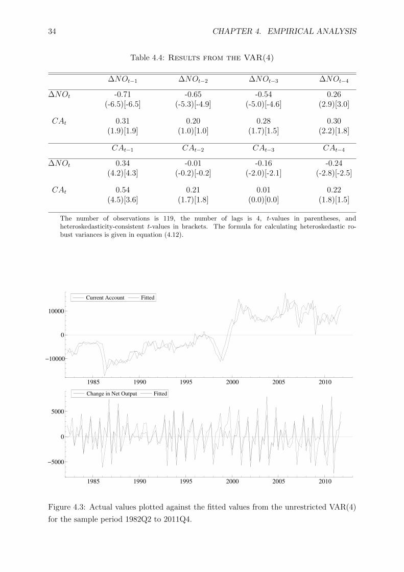
4.3 The unrestricted VAR(4) . . . . . . . . . . . . . . . . . . . . . . . . . 34
4.4 The current account balance from the intertemporal model 36
4.5 The restricted VAR(4) . . . . . . . . . . . . . . . . . . . . . . . . . . 38
4.6 The residuals from the VAR(4) . . . . . . . . . . . . . . . . . . . . . 41
5.1 The extended VAR(5) . . . . . . . . . . . . . . . . . . . . . . . . . . . 52
vii

viii LIST OF FIGURES

List of Tables
3.1 Results from the literature . . . . . . . . . . . . . . . . . . . . . . . 25
4.1 Quarterly moments . . . . . . . . . . . . . . . . . . . . . . . . . . . . . 28
4.2 Unit root test for the period 1981–2011 . . . . . . . . . . . . . . 30
4.3 Lag selection in the VAR . . . . . . . . . . . . . . . . . . . . . . . . . 33
4.4 Results from the VAR(4) . . . . . . . . . . . . . . . . . . . . . . . . . 34
4.5 Test for Granger causality in the VAR(4) . . . . . . . . . . . . . 35
4.6 The log-likelihood ratio test . . . . . . . . . . . . . . . . . . . . . . 39
4.7 The Lagrange-multiplier test . . . . . . . . . . . . . . . . . . . . . . 40
4.8 Testing for homoskedasticity . . . . . . . . . . . . . . . . . . . . . . 42
4.9 Testing for serial correlation . . . . . . . . . . . . . . . . . . . . . 43
4.10 Testing for normality . . . . . . . . . . . . . . . . . . . . . . . . . . . 44
4.11 The Wald test . . . . . . . . . . . . . . . . . . . . . . . . . . . . . . . . 46
5.1 Results from the extended VAR(5) . . . . . . . . . . . . . . . . . . 51
5.2 Granger causality in the extended VAR(5) . . . . . . . . . . . . . 52
ix

x LIST OF TABLES
Chapter 1
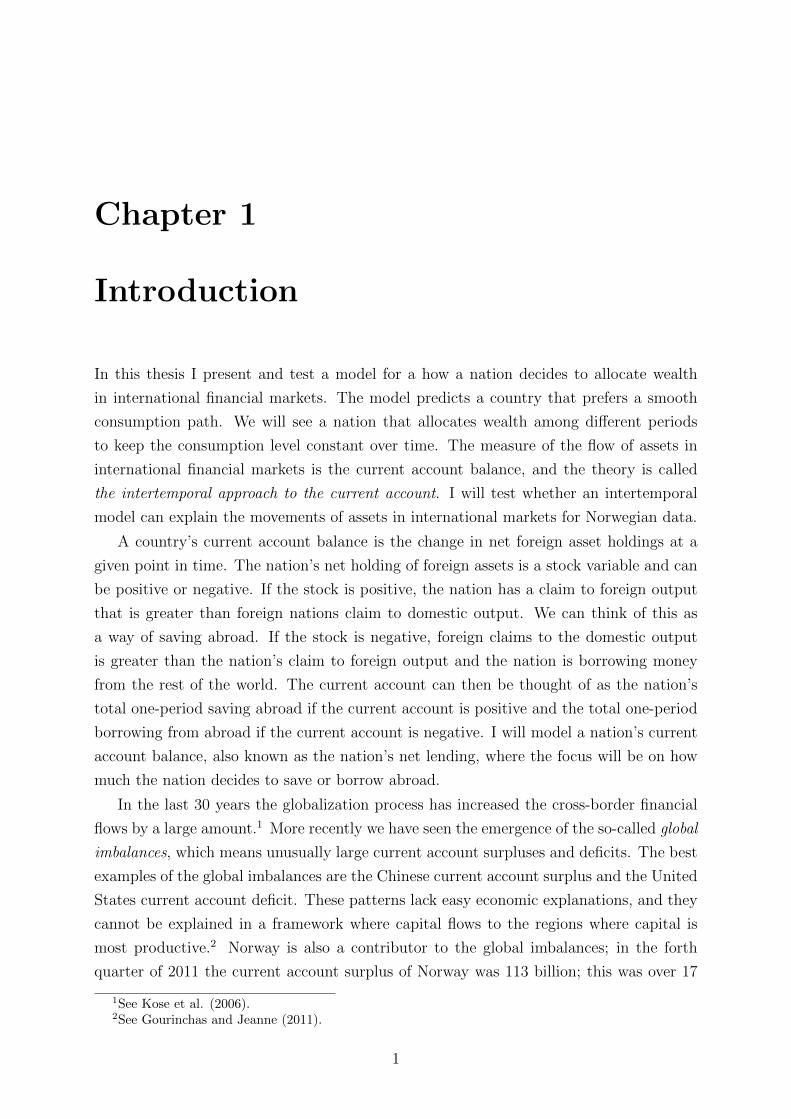
Introduction
In this thesis I present and test a model for a how a nation decides to allocate wealth
in international financial markets. The model predicts a country that prefers a smooth
consumption path. We will see a nation that allocates wealth among different periods
to keep the consumption level constant over time. The measure of the flow of assets in
international financial markets is the current account balance, and the theory is called
the intertemporal approach to the current account. I will test whether an intertemporal
model can explain the movements of assets in international markets for Norwegian data.
A country’s current account balance is the change in net foreign asset holdings at a
given point in time. The nation’s net holding of foreign assets is a stock variable and can
be positive or negative. If the stock is positive, the nation has a claim to foreign output
that is greater than foreign nations claim to domestic output. We can think of this as
a way of saving abroad. If the stock is negative, foreign claims to the domestic output
is greater than the nation’s claim to foreign output and the nation is borrowing money
from the rest of the world. The current account can then be thought of as the nation’s
total one-period saving abroad if the current account is positive and the total one-period
borrowing from abroad if the current account is negative. I will model a nation’s current
account balance, also known as the nation’s net lending, where the focus will be on how
much the nation decides to save or borrow abroad.
In the last 30 years the globalization process has increased the cross-border financial
flows by a large amount.1 More recently we have seen the emergence of the so-called global
imbalances, which means unusually large current account surpluses and deficits. The best
examples of the global imbalances are the Chinese current account surplus and the United
States current account deficit. These patterns lack easy economic explanations, and they
cannot be explained in a framework where capital flows to the regions where capital is
most productive.2 Norway is also a contributor to the global imbalances; in the forth
quarter of 2011 the current account surplus of Norway was 113 billion; this was over 17
1See Kose et al. (2006).2See Gourinchas and Jeanne (2011).
1

2 CHAPTER 1. INTRODUCTION
Norwegian Investment Abroad Foreign Investment in Norway
1995 2000 2005 2010
−250000
0
250000
500000
750000
1000000
Norwegian Investment Abroad Foreign Investment in Norway
Figure 1.1: Norwegian investment abroad and foreign investment in Norway. The valuesare in real 2008 million NOK.
percent of Norway’s gross domestic product that quarter.3 The objective of this paper is
to explain the current account balance for Norway, where I will focus on the intertemporal
consumption decision as the determinant of the current account.
In Figure 1.1 I plot Norwegian investment abroad, which is the change in Norwegian
asset holdings abroad, and I plot foreign investment in Norway, which is the change
in foreign nations asset holdings in Norway.4 The change in Norwegian asset holdings
abroad is negative in one period; that is in 2009. It is plausible to think this has to do
with the financial crises, and the reduction in asset holdings is a result from a devaluation
of the holdings of foreign assets. The difference between Norwegian investment abroad
and foreign investment in Norway is the net lending.5 Norway’s net lending is plotted in
Figure 1.2. We can see the increase in both foreign lending and borrowing over time up
until the financial crisis in 2007. At the same time we see that net lending has been high
and somewhat stable since the beginning of year 2000.
The basis for the theoretical model is the permanent income hypothesis developed by
3The data is from Statistics Norway; see http://www.ssb.no/ur en/.4The data in Figure 1.1 and Figure 1.2 is from Statistics Norway, and can be found under the financial
account in the balance of payments; see http://www.ssb.no/ur en/.5In the data, there are some discrepancies between the difference between Norwegian investment
abroad and foreign investment in Norway, and the net lending because of undistributed financial trans-actions and statistical errors.

3
Net Lending
1995 2000 2005 2010
0
50000
100000
150000
200000
250000
300000
350000
Net Lending
Figure 1.2: Net lending for Norway. The values are in real 2008 million NOK.
Friedman (1957). The permanent income hypothesis is going against the traditional Key-
nesian view where consumption is a constant share of disposable income in a given period.
Instead Friedman theorized that consumption is a share of permanent lifetime income.
The theory implies that temporary income shocks do not affect consumption much since
temporary shocks has a marginal effect on lifetime income whereas permanent shocks
affects consumption one-to-one. Hall (1978) finds evidence in favor of the permanent
income hypothesis for postwar data for the United States. In Hall’s paper consumption
follows a random walk and this theory is often refereed to as Hall’s random walk hypoth-
esis. This is a result from an Euler equation approach to describe the development of
consumption. The Euler equation approach means that economic relations are derived
from a mathematical optimization problem. This approach was a response to the Lucas
critique where Lucas argued that predicting the effects of economic policy on the basis
of historical observed relationships alone was a bad idea.6 Instead Lucas suggested we
should try to model the determinants of individual behavior such as preferences, technol-
ogy, initial resources etc. This critique encouraged macroeconomic modeling to be based
on microeconomic foundations. I will follow this approach and use an Euler equation to
model consumption as a random walk.
While Hall is saying something about individual consumption and saving behavior
within a country, I am going to analyze the permanent income hypothesis on an interna-
6See Lucas (1976).
4 CHAPTER 1. INTRODUCTION
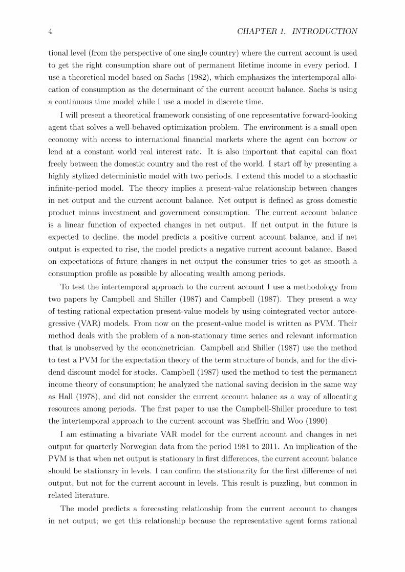
tional level (from the perspective of one single country) where the current account is used
to get the right consumption share out of permanent lifetime income in every period. I
use a theoretical model based on Sachs (1982), which emphasizes the intertemporal allo-
cation of consumption as the determinant of the current account balance. Sachs is using
a continuous time model while I use a model in discrete time.
I will present a theoretical framework consisting of one representative forward-looking
agent that solves a well-behaved optimization problem. The environment is a small open
economy with access to international financial markets where the agent can borrow or
lend at a constant world real interest rate. It is also important that capital can float
freely between the domestic country and the rest of the world. I start off by presenting a
highly stylized deterministic model with two periods. I extend this model to a stochastic
infinite-period model. The theory implies a present-value relationship between changes
in net output and the current account balance. Net output is defined as gross domestic
product minus investment and government consumption. The current account balance
is a linear function of expected changes in net output. If net output in the future is
expected to decline, the model predicts a positive current account balance, and if net
output is expected to rise, the model predicts a negative current account balance. Based
on expectations of future changes in net output the consumer tries to get as smooth a
consumption profile as possible by allocating wealth among periods.
To test the intertemporal approach to the current account I use a methodology from
two papers by Campbell and Shiller (1987) and Campbell (1987). They present a way
of testing rational expectation present-value models by using cointegrated vector autore-
gressive (VAR) models. From now on the present-value model is written as PVM. Their
method deals with the problem of a non-stationary time series and relevant information
that is unobserved by the econometrician. Campbell and Shiller (1987) use the method
to test a PVM for the expectation theory of the term structure of bonds, and for the divi-
dend discount model for stocks. Campbell (1987) used the method to test the permanent
income theory of consumption; he analyzed the national saving decision in the same way
as Hall (1978), and did not consider the current account balance as a way of allocating
resources among periods. The first paper to use the Campbell-Shiller procedure to test
the intertemporal approach to the current account was Sheffrin and Woo (1990).
I am estimating a bivariate VAR model for the current account and changes in net
output for quarterly Norwegian data from the period 1981 to 2011. An implication of the
PVM is that when net output is stationary in first differences, the current account balance
should be stationary in levels. I can confirm the stationarity for the first difference of net
output, but not for the current account in levels. This result is puzzling, but common in
related literature.
The model predicts a forecasting relationship from the current account to changes
in net output; we get this relationship because the representative agent forms rational

5
expectations about future changes in output and based on these expectations choose the
current account that gives a smooth consumption path. The forecasting relationship is
confirmed in the data. We can see causality from the current account balance to changes
in net output, but not from changes in net output to the current account.
It is possible to evaluate the model graphically by calculating the predicted current
account series from the PVM and plotting this against the actual current account se-
ries. The result is convincing, the predicted and actual series are close; the correlation
coefficient between the actual and predicted series is equal to 0.97. The variance of the
actual series divided by the variance of the predicted series is 0.75, so the actual series
is more volatile than what the model predicts. The overall graphical picture is a model
that tracks the data well.
The PVM is a nested version of a general VAR and I find the restrictions on this
general VAR that gives the PVM. I report three formal tests of the PVM. First a log-
likelihood ratio test, which evaluates whether the restrictive VAR is a valid simplification
of the general VAR. Second I report a test suggested by Campbell (1987), this is a test of
the restrictions on the parameter matrix from the VAR based on information at time t−1.
With information at time t−1, the forecast for the present value of changes in net output
should be equal on time t and t− 1. The third test is a Wald test; this is a direct test of
whether the estimated parameter values from the VAR satisfy the restrictions implied by
theory. All three tests reject the PVM.
The paper proceeds as follows: Chapter 2 presents the theoretical framework for the
intertemporal approach to the current account, Chapter 3 gives a background on the
empirical methodology and a review of related literature, Chapter 4 presents the empirical
approach and my findings for Norwegian data, Chapter 5 discusses causes for why the
model is rejected and presents some empirical results unrelated to the theoretical model,
while Chapter 6 concludes.

6 CHAPTER 1. INTRODUCTION

Chapter 2
Theoretical framework
The basis for the model presented in this chapter is the model developed by Sachs (1982).
The focus in this model is the intertemporal allocation of wealth among different periods
in time. This chapter will present a discrete time theoretical model for the intertempo-
ral approach to the current account. We will see a model that implies a present-value
relationship between the current account and expected changes in net output.
A great advantage in an open economy is the possibility to lend too, and borrow from,
the rest of the world. In a particular period a nation can decide how much to spend and
how much to save. It is possible to make a consumption plan where consumption deviates
from the disposable domestic income in the periods to come. This form of resource
exchange across time is called intertemporal trade. The size of this intertemporal trade
is measured as the current account of the balance of payments. The country’s current
account balance is the net increase in foreign asset holdings and is defined as
CAt ≡ Bt+1 −Bt, (2.1)
where Bt is the holdings of foreign assets at time t. The current account is a flow variable
and is a measure of the change in total holdings of foreign assets. The total amount of
foreign assets, Bt, is a stock variable. An alternative formulation for the current account
is given by
CAt = Yt + rBt − Ct −Gt − It, (2.2)
where Yt is gross domestic product, Ct is private consumption, Gt is government con-
sumption, It is investment, and r is the word real interest rate. Equation (2.2) can be
interpreted as the one-period budget constraint where Yt+ rBt is the gross national prod-
uct, which can be thought of as total one-period income for the economy, and Ct+Gt+ It
is total one-period domestic expenditure for the economy. The intertemporal trade is
used to fill the potential gap between domestic expenditure and domestic income. When
CAt > 0 the current account balance is in surplus and the country is a creditor, and if
CAt < 0 the current account balance is in deficit and the country is a debtor.
7

8 CHAPTER 2. THEORETICAL FRAMEWORK
The standard Keynesian view of the current account is treating it as the nation’s net
export. When the production in the economy is above national demand, the country is a
net exporter. If national output is below national demand the country is a net importer.
This view is not in any way contradicting the view in this thesis, but my approach will
be to treat the current account balance as the difference between national saving and
national investment. In this framework imports and exports are not directly observed. In
the net export approach the usual focus is on the determinants of imports and exports
such as the relative competitiveness of the nation, the trade determinants does not play
any direct role in the model I will use.
To model the current account I use the theory of forward-looking rational agents,
which on the basis of expectations of the future decides how much to save and invest.
Actually, the model will not include a production side, so investment is treated as an
exogenous variable, and the only decision variable is how much to save. If our rational
agents are a good approximation to the actual population, we may be able to model
the fluctuations in the current account balance based on a model of their behavior. The
foundations for the model presented in this chapter are from the book by Obstfeld and
Rogoff (1996), Chapter 1 and 2.
2.1 A model with two periods and no uncertainty
Let us consider a small open endowment economy with one representative consumer. In an
endowment economy the production side is treated as exogenous. First, let the economy
consist of two periods; the first period represents the present and the second period the
future. I extend the model to an infinite-period model in the next section. The consumer
has access to international financial markets and can borrow or lend at the constant risk-
free world real interest rate. There is one good in the economy, and the good lasts for
one period only. For now let Gt = It = 0. There is no uncertainty, so the output in both
periods is known for sure to the consumer in the first period. By combining equation
(2.1) and (2.2) the one-period budget constraint can be written as
Ct +Bt+1 = (1 + r)Bt + Yt, for t = 1, 2. (2.3)
If we combine the one-period budget constraints in equation (2.3) for both periods we
find the intertemporal budget constraint where B3 is equal to 01
C1 +C2
1 + r= (1 + r)B1 + Y1 +
Y2
1 + r. (2.4)
1Non-satiation and the no-Ponzi game condition that ensures B3 = 0 is discussed in detail for theinfinite-period model in the next section.

2.1. A MODEL WITH TWO PERIODS AND NO UNCERTAINTY 9
This constraint ensures that the present value of all consumption equals the present value
of all income. The term (1+r)Bt is the return from foreign asset holdings obtained before
period 1, and can be consumed during period 1 and 2. All consumption sets C1, C2that satisfies equation (2.4) are feasible to the consumer. The variables B1, r, Y1, and Y2
are exogenous and known to the consumer in both periods. The only choice the consumer
can make is how to allocate the resources between consumption in the two periods.
To figure out what consumption set the consumer chooses we need to introduce pref-
erences. Let the preferences be time-separable; in period 1 the consumer has the following
lifetime utility level
U1 = u(C1) + ρu(C2), 0 < ρ < 1, (2.5)
where ρ is the subjective discount factor and u(·) is a one-period utility function where
u′ > 0 and u′′ ≤ 0. The consumer has perfect foresight and the optimal consumption set
is the solution to maximizing equation (2.5) subject to equation (2.4) with respect to C1
and C2. From equation (2.3) we can see that B2 determines both C1 and C2 where
C1 = (1 + r)B1 + Y1 −B2 and C2 = (1 + r)B2 + Y2.
Since B1, Y1, and Y2 are exogenous, the only decision variable for the consumer is B2.
From equation (2.1) the consumption set C1, C2 determines the current account and
Figure 2.1: The budget line gives the possible combinations of future and current con-sumption.
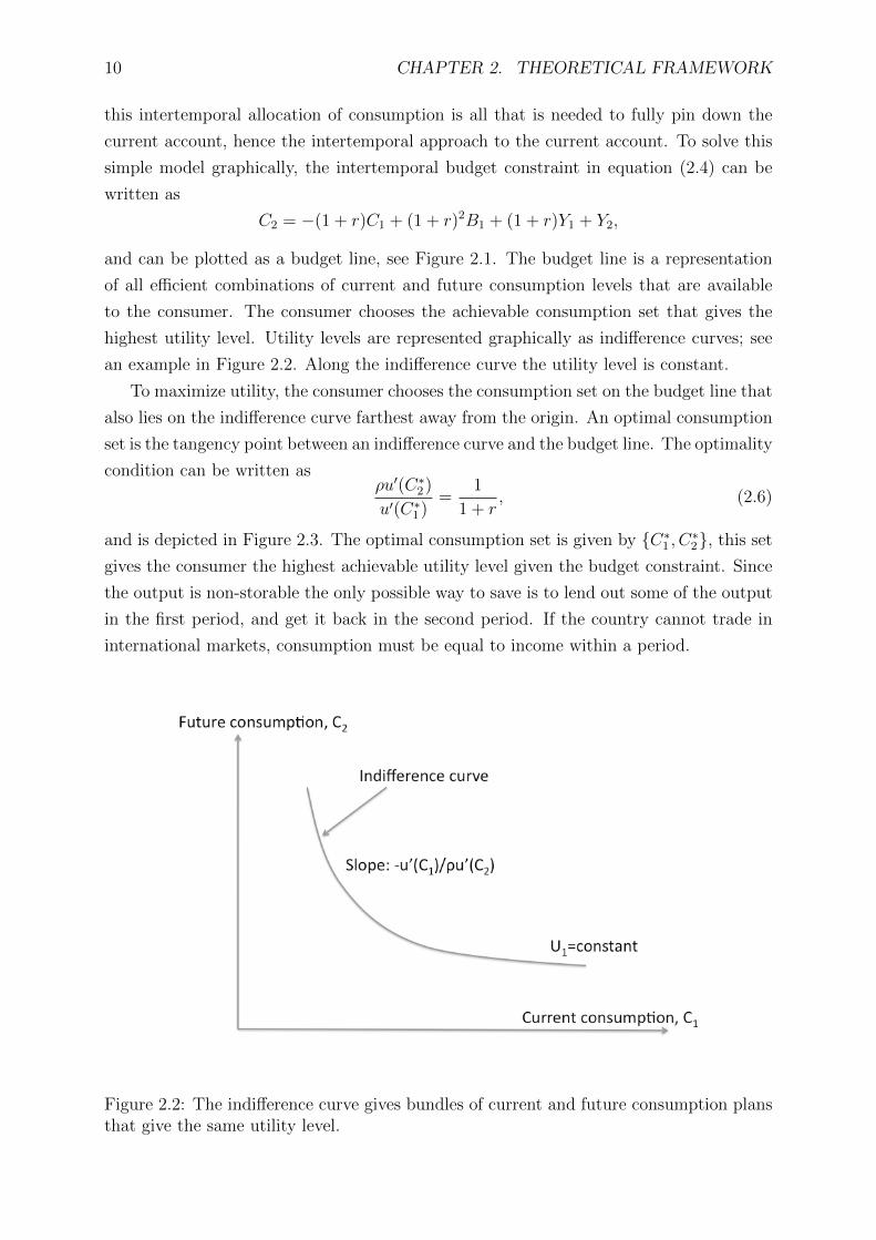
10 CHAPTER 2. THEORETICAL FRAMEWORK
this intertemporal allocation of consumption is all that is needed to fully pin down the
current account, hence the intertemporal approach to the current account. To solve this
simple model graphically, the intertemporal budget constraint in equation (2.4) can be
written as
C2 = −(1 + r)C1 + (1 + r)2B1 + (1 + r)Y1 + Y2,
and can be plotted as a budget line, see Figure 2.1. The budget line is a representation
of all efficient combinations of current and future consumption levels that are available
to the consumer. The consumer chooses the achievable consumption set that gives the
highest utility level. Utility levels are represented graphically as indifference curves; see
an example in Figure 2.2. Along the indifference curve the utility level is constant.
To maximize utility, the consumer chooses the consumption set on the budget line that
also lies on the indifference curve farthest away from the origin. An optimal consumption
set is the tangency point between an indifference curve and the budget line. The optimality
condition can be written asρu′(C∗2)
u′(C∗1)=
1
1 + r, (2.6)
and is depicted in Figure 2.3. The optimal consumption set is given by C∗1 , C∗2, this set
gives the consumer the highest achievable utility level given the budget constraint. Since
the output is non-storable the only possible way to save is to lend out some of the output
in the first period, and get it back in the second period. If the country cannot trade in
international markets, consumption must be equal to income within a period.
Figure 2.2: The indifference curve gives bundles of current and future consumption plansthat give the same utility level.

2.1. A MODEL WITH TWO PERIODS AND NO UNCERTAINTY 11
In Figure 2.3 total autarky income or wealth is given by Y1, Y2, and in this particular
case the optimal consumption level in the present lies to the right of this point. In this case
national wealth in the first period Y1 is lower than the optimal consumption level C∗1 . To
achieve the optimal consumption level the representative consumer runs a current account
deficit the first period, CA1 < 0, so consumption in this period is higher than domestic
wealth. This borrowed consumption must be repaid in the future, and we can see that
consumption in the future, C∗2 , is lower than future national wealth, Y2. If international
markets are closed in all periods we have Yt = Ct for t = 1, 2.
Figure 2.3: This figure gives the optimal consumption set given by C∗1 , C∗2. The exoge-nous variables and the consumer’s preferences decide the size and the sign of the currentaccount.
An important measure in this model is the elasticity of intertemporal substitution.
This is a measure of the responsiveness of the intertemporal allocation of consumption
to changes in the real interest rate. A higher interest rate may make the agent want to
consume less and save more due to the increased return on savings, this is a substitution
effect. It is also possible that the agent want to increase consumption due to the higher
return on what he or she already saves, this is an income effect. The total effect on con-
sumption from a change in the interest rate is measured by the elasticity of intertemporal
substitution. If the elasticity of intertemporal substitution is constant over time, it can
12 CHAPTER 2. THEORETICAL FRAMEWORK
be written as2
σ = − u′(C)
Cu′′(C).
Graphically, a change in the real interest rate will rotate the budget line around CMAX1 in
Figure 2.3, and the effect of this change on the current account depends on the particular
form of the indifference curve.
The model in this section is giving us a way of thinking about how a nation can
allocate wealth between the present and the future. Let the subjective discount factor
ρ be equal to the real discount factor 1/(1 + r), so ρ(1 + r) = 1, then the marginal
utility in the two periods must be equal in the optimal allocation (see equation (2.6)),
and the model predicts full consumption smoothing. We can look at what happens if the
income changes. Assume we are in the first period and we have an optimal consumption
allocation, then imagine an increase in the income that can be of two types: First, let
the income be permanently higher so the income is equally larger in both periods. Then,
to get to the new optimal allocation, consumption in both periods must be increased by
the same amount, this can be done without interacting in international financial markets,
and a permanent higher income does not affect the current account balance. The second
type is an increase in income in one of the two periods. To get an equal consumption level
in both periods the consumer must transfer wealth from the period with higher income
to the period with unchanged income. The only way to do this is to borrow or lend in
international financial markets. The consumer must borrow if income has increased in the
second period and lend if it has increased in the first. We see that shocks to the income
in one period only, can create large fluctuation in the current account.
2The elasticity of intertemporal substitution is defined as the percentage change in consumption growthto a percentage point change in the interest rate, this can be written as
σ =d log
(C2
C1
)dr
.
By taking logs of the optimality condition in equation (2.6) we get log(1 + r) = log u′(C1)ρu′(C2)
, by approxi-
mating this expression we get r = log u′(C1)− log u′(C2) and differentiating gives
dr =u′′(C1)C1
u′(C1)d logC1 −
u′′(C2)C2
u′(C2)d logC2.
If u′′(C1)C1/u′(C1) = u′′(C2)C2/u
′(C2) = u′′(C)C/u′(C), we have
d log(C2
C1
)dr
= − u′(C)
Cu′′(C).

2.2. A MODEL WITH AN INFINITE NUMBER OF PERIODS 13
2.2 A model with an infinite number of periods
The two-period model is good for intuition, but is obviously far from reality. To get a
model that can be tested against actual data some changes are needed. The infinite-
period model presented in this section consists of the same building blocks as the two-
period counterpart. The main elements are the time-separable utility function and the
budget constraint. The model still consists of one representative consumer; the consumer
is infinitely lived and is getting utility from consumption. By introducing uncertainty, the
representative consumer maximizes the expected value of lifetime utility given by
Ut = Et
∞∑s=t
ρs−tu(Cs)
, 0 < ρ < 1, (2.7)
where Et is the expectation operator conditioned on the available information set at time
t. As before the economy consists of one asset, a risk-free bond B that pays the constant
world real interest rate r. If we open up for government spending and investment the
one-period budget constraint is given by
Ct +Gt + It +Bt+1 = (1 + r)Bt + Yt, for all t. (2.8)
When external borrowing is permitted, the total amount of borrowing needs to be re-
stricted to prevent a potential Ponzi scheme. A Ponzi scheme is when new debt is issued
to repay old debt and this process is continued so the debt never gets repaid. In the two-
period model all the debt must be repaid in the second period so B3 ≥ 0. The no-Ponzi
game condition for the infinite-period case can be stated as
limi→∞
(1
1 + r
)iBt+i+1 ≥ 0. (2.9)
The concave utility function ensures that the utility level is always increasing in con-
sumption, this is called non-satiation, therefore it is optimal to consume everything that
is available to the consumer during the lifetime and leave no resources unused when the
life is over. In the two-period case this is satisfied if B3 ≤ 0. For the infinite-period case,
consuming everything during the lifetime is harder to picture, but both the no-Ponzi con-
dition and the non-satiation condition is satisfied if equation (2.9) holds with equality,
that is
limi→∞
(1
1 + r
)iBt+i+1 = 0. (2.10)
The consumer’s optimization problem is to maximize equation (2.7) subject to equation
(2.8) and (2.9). If we solve equation (2.8) for the consumption level and substitute into
equation (2.7) we get

14 CHAPTER 2. THEORETICAL FRAMEWORK
Ut = Et
∞∑s=t
ρs−tu((1 + r)Bs −Bs+1 + Ys −Gs − Is)
.
The representative consumer has one decision variable, which is to choose how much to
save or borrow in international markets. This is equivalent to the two-period case where
the consumer decided B2, in this case the decision variable is Bt+1. If Ut is maximized
with respect to Bt+1 the first order condition is given by the intertemporal Euler equation
Etu′(Cs) = (1 + r)ρEtu′(Cs+1) for s = 0, 1, 2, . . . , (2.11)
which is the same condition as the optimality condition for the two-period model given
by equation (2.6) except we now allow for uncertainty. The Euler equation is a condition
that ensures that no intertemporal shifts in consumption can give the consumer a higher
utility level. To get a solution for the consumption level, further specifications are needed.
First let (1 + r)ρ = 1. I also use a quadratic utility function given by
u(Ct) = Ct +a
2C2t ,
where a is a constant. Then, put the quadratic utility function into the Euler equation
given in (2.11) and solve for the consumption level, and we get
Ct = Et[Ct+s] for s = 0, 1, 2, . . . . (2.12)
With a quadratic utility function, consumption will follow a random walk. The best
predictor of next period consumption is the consumption level this period. We get the
same consumption level in all periods because the subjective discount rate is equal to the
real discount rate and there is no tilting of consumption to the present or to the future.
If we allow for consumption tilting, we get a consumption profile that is increasing or
decreasing over time in a predictable pattern, relaxing the assumption that the subjective
discount rate is equal to the real discount rate will not alter the main conclusions in this
model.
To see how this result affects the current account we need to find the intertemporal
budget constraint. To find the intertemporal budget constraint for the infinite-period
case we are summing the one-period budget constraint, given in equation (2.8), over all
periods and discounting to period t values, this gives
∞∑s=t
(1
1 + r
)s−tCs +Gs + Is +Bs+1 =
∞∑s=t
(1
1 + r
)s−t(1 + r)Bs + Ys . (2.13)
2.2. A MODEL WITH AN INFINITE NUMBER OF PERIODS 15
If we use equation (2.10), equation (2.13) can be rewritten as3
∞∑s=t
(1
1 + r
)s−tCs = (1 + r)Bt +
∞∑s=t
(1
1 + r
)s−tYs −Gs − Is .
If we substitute for the consumption level from equation (2.12) we get
Ct
∞∑s=t
(1
1 + r
)s−t= (1 + r)Bt +
∞∑s=t
(1
1 + r
)s−tYs −Gs − Is .
By taking expectations of this equation we get4
Ct =r
1 + r
[(1 + r)Bt +
∞∑s=t
(1
1 + r
)s−tEt(Ys −Gs − Is)
]. (2.14)
This equation implies certainty equivalence. If we define net output as NOt ≡ Yt−Gs−Is,consumption is determined as if future net output is known for sure. Certainty equivalence
means that the consumer acts as if there was no uncertainty even when there is. This is
because the utility function is quadratic so marginal utility is linear, and the consumer
is risk neutral.5 Equation (2.14) is an example of the permanent income hypothesis ; the
consumer want to consume a given share of the present value of net output in every period
and the consumption plan is perfectly smooth. In this type of model it is important
to distinguish between permanent and transitory shocks. Let a permanent shock be a
permanent higher income in future periods, and let the consumer anticipate the shock.
Then, the consumer’s optimal strategy is to increase consumption in every period to adjust
to the higher value of total lifetime income, since the shock is permanent this can be done
without using the current account. On the other hand if the shock is temporary, the
present value of lifetime income will not change much. Then, to smooth consumption the
consumer will choose to save almost all of the temporary higher income and run a current
account surplus. The consumption every period will only increase by a small amount.
The model implies that transitory shocks to the economy will create large fluctuations in
3Where I use
∞∑s=t
(1
1 + r
)s−t(1 + r)Bs −Bs+1
= [(1 + r)Bt −Bt+1] +
(1
1 + r
)[(1 + r)Bt+1 −Bt+2] +
(1
1 + r
)2
[(1 + r)Bt+2 −Bt+3] + . . .
= (1 + r)Bt − limi→∞
(1
1 + r
)iBt+i+1 = (1 + r)Bt.
4Note that∞∑s=t
(1
1+r
)s−tis a geometric series such that
∞∑s=t
(1
1+r
)s−t= 1+r
r for r > 0.
5To see why the consumer is risk neutral note that E[u′(C)] = u′(E[C]) for a quadratic utility function.

16 CHAPTER 2. THEORETICAL FRAMEWORK
the current account, while permanent shocks have no effect.
In this model Yt, Gt, and It are treated as random variables and their present values
are given as permanent values. Let the one-period average permanent value for a random
variable at time t be given by Xt, and we can write
∞∑s=t
(1
1 + r
)s−tXs =
∞∑s=t
(1
1 + r
)s−tXs ⇒ Xt =
r
1 + r
∞∑s=t
(1
1 + r
)s−tXs.
If we use this notation, equation (2.14) can be rewritten as
Ct = rBt + EtYt + EtGt + EtIt. (2.15)
Then, substitute for Ct from equation (2.15) into equation (2.2), and we get
CAt = (Yt − EtYt)− (It − EtIt)− (Gt − EtGt),
and by using NOt = Yt − Gt − It we get
CAt = NOt − EtNOt. (2.16)
We can see from this equation that the current account in period t is determined by
the difference between net output and the expected average present value of future net
output. If we let the change in net output be defined as ∆NOt ≡ NOt−NOt−1, equation
(2.16) can be rearranged to the following model
CAt = −∞∑
s=t+1
(1
1 + r
)s−tEt∆NOs. (2.17)
The derivation of this expression can be found in Appendix A. Equation (2.17) is a PVM
for two variables, CAt and ∆NOt. The model states that the current account balance is
a linear function of the discounted value of expected changes in future income streams.
When the discounted value of future changes in net output is positive, the current account
balance should be negative. When we expect higher output in the future we should run a
current account deficit today. The current account is a linear function of expected future
changes in net output, and the model implies that if net output is stationary in first
differences the current account must be stationary in levels. Another important point can
be found by following Campbell (1987), where a testable implication based on information
at time t− 1 is given by
CAt −∆NOt − (1 + r)CAt−1 = −rεt, (2.18)
2.2. A MODEL WITH AN INFINITE NUMBER OF PERIODS 17
where εt is given by
εt ≡(
1
1 + r
) ∞∑s=t
(1
1 + r
)s−t[EtNOs − Et−1NOs] .
See Appendix B for the derivation of equation (2.18). At time t− 1, let εt = 0, this is the
case if the expected present value of future net output is equal at time t and t − 1, and
this should be true at time t− 1. Then, we have the following expression for the current
account
CAt = ∆NOt + (1 + r)CAt−1. (2.19)
If the agent is rational, equation (2.19) is the best prediction of the current account, and
we do not expect this prediction to be systematically wrong. At period t− 1, before the
realized net output next period is known, all the available information on the outcome
in the next period is used, and the best model for the next period current account is the
change in net output next period plus the gross current account this period. Since we
are using period t − 1 information, and the values of CAt and ∆NOt are known only in
expectation, a more intuitive formulation of equation (2.19) may be
Et−1CAt = Et−1∆NOt + (1 + r)CAt−1.
The current account is decided by the rational agent where the objective is to get a smooth
consumption path, which is done by adjusting external saving. Let us assume that net
output is above its permanent value, so the current account is in surplus. If we expect
net output next period (period t) to be at the same level as this period (period t− 1) the
current account should be equal in the two periods except the change in income from the
increase in interest income since the total amount of foreign assets has increased. To hold
disposable income constant when ∆NOt is expected to be zero, the current account in
period t should equal (1 + r)CAt−1. If we expect net output to change from this period
to the next, we need to compensate for this change by changing the current account to
keep consumption constant. If we expect net output to be higher in period t, ∆NOt > 0,
all of this higher net output should be saved and this is what the model predicts. This
argument is parallel for a nation with a current account deficit.
The main result from this chapter is the PVM given in equation (2.17). I present
equation (2.18) because this formulation can easily be tested, and we will se this result in
the Lagrange-multiplier test in section 4.7.2. These observations and other implications
of the model in equation (2.17) are examined for Norwegian data in Chapter 4.

18 CHAPTER 2. THEORETICAL FRAMEWORK
Chapter 3
Empirical background
In this chapter I will look at the background for the empirical part of my thesis. I
use the empirical methodology developed by Campbell and Shiller (1987) and Campbell
(1987), their method is to use vector autoregressive (VAR) models to test present-value
relationships. The advantage with the Campbell-Shiller method is that they deal with
the problem of non-stationarity in the data and the possibility that the econometrician
lack relevant information that the rational agent is assumed to use when predicting the
future. A VAR with no contemporaneous terms on the right-hand side can easily be
estimated by the ordinary least squares (OLS) procedure.1 OLS is valid if the model
to be estimated satisfies the classical linear regression (CLR) model. In this chapter I
present some background for the Campbell-Shiller method, the assumptions behind the
CLR model, some principles of forecasting by using a VAR, and some theory for empirical
testing of a PVM. I also present some results from other literature that evaluates the
validity of the intertemporal approach to the current account for other countries.
3.1 The empirical methodology
Campbell and Shiller (1987) and Campbell (1987) develop a method for testing PVMs
by estimating cointegrated variables in a VAR. The first paper by Campbell and Shiller
(1987) use the method to test the rational expectations theory of the term structure
of bonds and the PVM for stock prices. Campbell (1987) tests the permanent income
hypothesis (PIH) for consumption on the national level where he differentiates between
labor income and capital income, Campbell is investigating saving as national capital
accumulation, while I will look at saving as foreign asset allocation. Campbell’s paper lie
close to what I will do and I will take a brief look at it in the next paragraph.
If the PIH is true, the theory states that saving, which means buying capital, should
1A contemporaneous right-hand side variable is a variable that is varying at the same time as the left-hand side variable; if the system has contemporaneous right-hand side variables, we have a simultaneousequation system.
19
20 CHAPTER 3. EMPIRICAL BACKGROUND
be equal to the discounted sum of future declines in labor income so consumption is kept
constant over the lifetime, and as Campbell writes, “they save for a rainy day.” The PIH
predicts that saving contains all available information on future developments of labor
income. To test this implication from the PIH, Campbell estimates a VAR for saving and
the change in labor income, and he writes:2
If the PIH is true, saving is the optimal forecast of the present value of future
declines in labor income, conditional on agents’ information; therefore the
unrestricted VAR forecast of this present value should equal saving.
This is the basis for the empirical part in my thesis, the model in Chapter 2 implied that
the current account is equal to the discounted sum of future changes in net output, hence
the current account balance should be equal to the forecast of the present value of changes
in net output. Campbell and Shiller show how this implication can be tested formally,
and I follow their approach in Chapter 4.
A VAR system consists of two or more variables, all variables are treated symmetrically
and every component depends on own lagged values and lagged values of all the other
components in the system. In a VAR all variables are endogenous and we can say that
everything depends on everything. A VAR of order p, written as VAR(p), means a
system consisting of one equation for each endogenous variable, and the dependent variable
depends on p lags of all the components in the VAR. A VAR(p) with two endogenous
variables can be formulated in the following way
y1t = c1 + b11y1,t−1 + b12y1,t−2 + · · ·+ b1py1,t−p + a11y2,t−1 + a12y2,t−2 + · · ·+ a1py2,t−p + u1t
y2t = c2 + b21y1,t−1 + b22y1,t−2 + · · ·+ b2py1,t−p + a21y2,t−1 + a22y2,t−2 + · · ·+ a2py2,t−p + u2t.
This is called a bivariate system where the endogenous variables are y1t and y2t, the
a’s, b’s and c’s are parameters, and u1t and u2t are residuals. In a VAR all endogenous
variables depend on predetermined lagged values of all the variables in the VAR, and all
the right-hand side variables in the system are exogenous. This is a general strength of
a VAR, when all right-hand side variables are exogenous there can be no feedback from
the left-hand side to the right-hand side and simultaneity bias is not an issue.
In the intertemporal model the current account is used by the agent to absorb tempo-
rary fluctuations in net output; if this theory holds, the agent chooses the current account
balance in a given period on the basis of the best predictions of future developments in
net income. The current account then contains all available information for future de-
velopments in net income and can be used by the econometrician to construct estimates
of changes in net output in the future. The rational agent’s information, which is only
observed through the realized values of the current account, is used to forecast changes
2See Campbell (1987), pp. 1251.

3.2. THE CLASSICAL LINEAR REGRESSION MODEL 21
in net output. It follows that relevant variables that are omitted from the VAR is no
problem as long as lagged values of the current account is included. So at least in theory,
omitted variables are not a problem when using this method.
In section 3.3, I demand that the data used for forecasting should be stationary, but
this is not always the case. Campbell and Shiller show how to transform a model so the
right-hand side variable in a PVM is in first differenced form while the left-hand side
variable is in levels. Appendix A shows this transformation for the intertemporal model
where net output can be included in first differenced form, this is important since we
expect net output to have a unit root.
3.2 The classical linear regression model
A general VAR can be estimated equation by equation using OLS. OLS is a method for
estimating the parameters in a model; the method is based on choosing the parameters
for the model that minimizes the sum of squared residuals (SSR). In regression analysis
some assumptions must be fulfilled for the OLS estimates to be valid. I will present the
assumptions for the classical linear regression (CLR) model. The CLR model is only valid
if we have access to a sample that has the exact distribution of the population we want
to explain; this is usually not satisfied, but can often be solved by using large sample
theory. In large sample theory the asymptotic properties of a sample when the number of
observations is getting large are approaching the properties of the whole population and
this is used to derive the model. I will not go into large sample theory in this thesis.3 The
CLR assumptions are given by:
Assumption 1 (linearity):
The regression model can be written as
yt = b1x1t + b2x2t + · · ·+ bKxKt + ut (t = 1, 2, . . . , T ),
where the b’s are the parameters to be estimated, y are the variable we are modeling, the
x’s are the explanatory variables and u is an error term. There are K regressors and T
observations.
Assumption 2 (strict exogeneity):
The error has an expected value equal to zero for any value of the explanatory variables,
this can be written as
E(ut|x11, x12 . . . , x1T , x21, . . . , x2T , . . . , xK1, . . . , xKT ) = 0 (t = 1, 2, . . . , T ).
3For details on the CLR model and large sample theory see Hayashi (2000), Chapter 1 and 2.

22 CHAPTER 3. EMPIRICAL BACKGROUND
Assumption 3 (no perfect multicollinearity):
There are none exact linear relationships among the explanatory variables.
Assumption 4 (homoskedasticity):
The error terms has a constant variance dependent on any value of the explanatory vari-
ables, this can be written as
E(u2t |x11, x12 . . . , x1T , x21, . . . , x2T , . . . , xK1, . . . , xKT ) = constant > 0 (t = 1, 2, . . . , T ).
Assumption 5 (no autocorrelation):
There is no correlation between the residuals, this can be written as
E(utuτ |x11, x12 . . . , x1T , x21, . . . , x2T , . . . , xK1, . . . , xKT ) = 0 (t, τ = 1, 2, . . . , T ; t 6= τ).
Assumption 6 (normality):
The distribution of the error terms conditional on
x11, x12 . . . , x1T , x21, . . . , x2T , . . . , xK1, . . . , xKT is jointly normal.
The first assumption states that the regression model must be a linear function of the
regressors. The second assumption demands the regressors to be exogenous, which means
determined outside the model. In a VAR all regressors are predetermined so this assump-
tion holds. Assumption 3 is about multicollinearity, we have perfect multicollinearity if
two or more regressors are perfectly correlated. In the case of perfect multicollinearity
the model is not identified and cannot be estimated. Assumption 4 is about the absence
of heteroskedasticity, which means the variance of the residuals must be constant. As-
sumption 5 of no autocorrelation states that the correlation between any pair of residuals
should be 0 (except for the same two residuals, correlation between the same two residuals
is equal to the variance and is covered in assumption 4). Autocorrelation may be a sign
of a misspecified model where for example too few lags are included. The last assumption
is about the normality of the distribution of the error terms. The normality assumption
does not matter for the efficiency of the estimator, but it is important for standard test-
ing procedures to be valid. For a regression where assumptions 1–5 hold, the estimators
are both unbiased and consistent, and OLS produces the best linear unbiased estimators
(BLUE).4
The first three assumptions will not be discussed further, and they are expected to
hold. I will investigate the last three assumptions for Norwegian data in section 4.8.
4See Hayashi (2000), Chapter 1.

3.3. FORECASTING USING A VAR 23
3.3 Forecasting using a VAR
To test the PVM, I need a forecast for changes in net output. In this section I will
present some principles of forecasting. Assume we have access to two data processes
given by y1tTt=1 and y2tTt=1. To make the arguments simple I will assume that the data
processes can be explained by a VAR(1). The model for explaining y1t and y2t can be
written as
y1t = c1 + b1y1,t−1 + a1y2,t−1 + u1t
y2t = c2 + b2y1,t−1 + a2y2,t−1 + u2t,
where y1t and y2t are the endogenous variables, y1t−1 and y2t−1 are the regressors, the a’s,
b’s and c’s are parameters to be estimated and, u1t and u2t are the residuals. If both
equations satisfy the CLR assumptions given above, the parameters can be estimated by
OLS. An important property for forecasting to make sense is that the variables need to be
stationary. For a non-stationary process the mean and variance of the series is varying over
time, which makes standard interference invalid. For a process to be covariance-stationary
the mean and the autocovariances should be constant and independent of time, this can
be written as
E(yit) = µi for all t and i = 1, 2
E[(yit − µ)(yit−j − µ)] = γij for all t and any j, and i = 1, 2,
where the E is an expectations operator, µi is the mean and γij is the covariance between
observation t and observation t − j.5 Then, we can estimate the VAR and determine
the coefficients. Next, the estimated coefficients can be used to predict the future; a one
period ahead forecast is given by
E(y1,t+1) = c1 + b1y1,t + a1y2,t
E(y2,t+1) = c2 + b2y1,t + a2y2,t.
A two period ahead forecast is given by
E(y1,t+2) = c1 + b1E(y1,t+1) + a1E(y2,t+1)
= c1 + b1c1 + b21y1,t + b1a1y2,t + a1c2 + a1b2y1,t + a1a2y2,t
E(y2,t+2) = c2 + b2E(y1,t+1) + a2E(y2,t+1)
= c2 + b2c1 + b2b1y1,t + b2a1y2,t + a2c2 + a2b2y1,t + a22y2,t.
5See Hamilton (1994), Chapter 3.

24 CHAPTER 3. EMPIRICAL BACKGROUND
For a VAR(1), we can in principle forecast values as far into the future we want by
following the procedure given above, as long as we have reliable estimated parameters and
the values y1t and y2t. This result can be generalized to a higher order VAR, but this will
get algebraically messy. In Chapter 4 I show a general formulation for forecasting with a
higher order VAR by using matrix notation.
3.4 Testing the PVM
The PVM derived in Chapter 2 is a nested version of a general VAR. To get to the PVM we
need to impose several restrictions on the parameters in the VAR. The method for testing
the theory is to evaluate the validity of the cross-equation restriction on the VAR implied
by the theory. Standard approaches for doing this are a Wald test, a log-likelihood ratio
test and a Lagrange-multiplier test, which are all asymptotically equal.6 I will present
all three tests because I believe they all give some valuable insights to the intertemporal
model.
For the log-likelihood ratio test, both the general and the restricted model are estimated
and the log-likelihood functions for both models are compared.7 The restrictions are valid
if we fail to reject the restricted model as a valid simplification of the general model. An
issue when using the log-likelihood ratio test is how to estimate the restricted model. The
restricted model is usually estimated by the maximum likelihood (ML) method. I will
not go into ML estimation in this thesis.8 I present the log-likelihood ratio test in section
4.7.1 where I present results from a ML estimation reported from the software package
OxMetrics.
The Lagrange-multiplier test, also known as the Score test, evaluates whether devia-
tions from the derived model is unpredictable at time t−1. We are not supposed to make
any systematic predictions about the future that deviates from the PVM (see equation
(2.19)) and this can be formally tested. The test is easy to implement by testing for
significance in the available information and whether we can outperform the theoretical
model. I present the test and its result in section 4.7.2.
The last test, the Wald test can be calculated using the results from the general VAR
alone, no additional regressions are necessary. This test is similar to a standard t-test
where the actual parameter values are compared to the hypothesized values. In addition
to a standard Wald test, I will report a heteroskedastic robust Wald test. I present the
Wald test and its results in section 4.9.
6See Engle (1984).7The calculation of the log-likelihood function is given in section 4.7.1.8See e.g. Hamilton (1994), Chapter 11.
3.5. RESULTS FROM RELATED LITERATURE 25
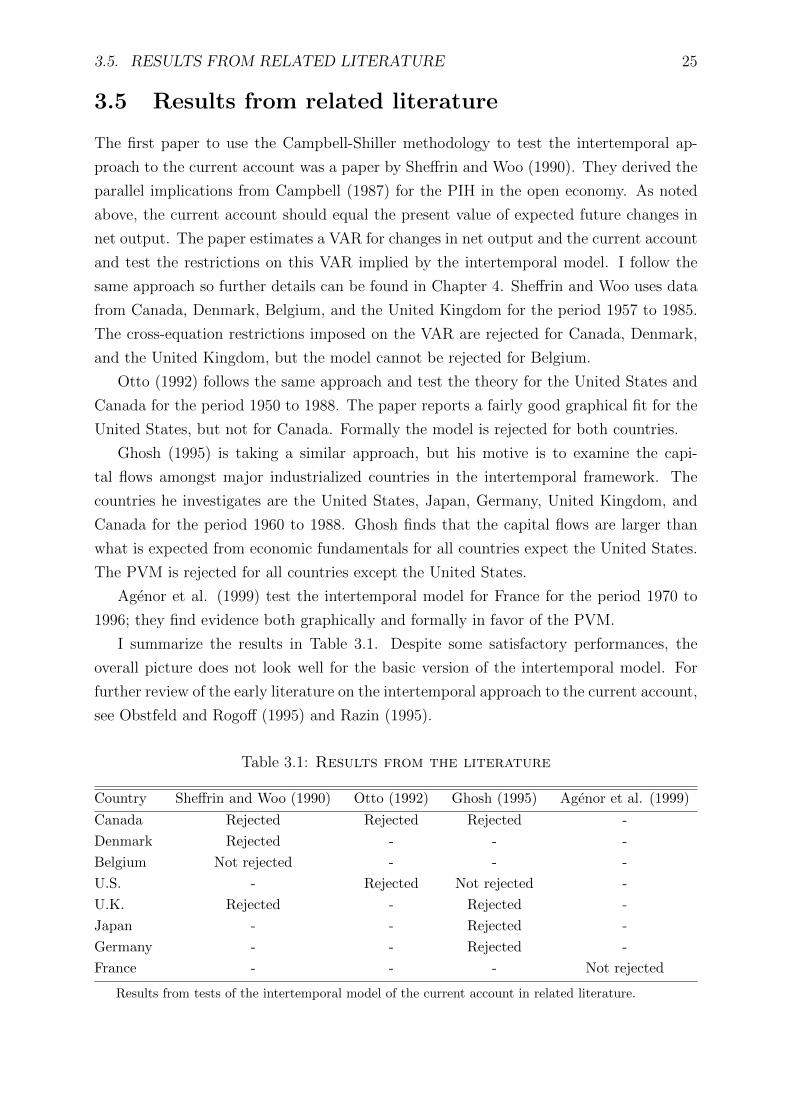
3.5 Results from related literature
The first paper to use the Campbell-Shiller methodology to test the intertemporal ap-
proach to the current account was a paper by Sheffrin and Woo (1990). They derived the
parallel implications from Campbell (1987) for the PIH in the open economy. As noted
above, the current account should equal the present value of expected future changes in
net output. The paper estimates a VAR for changes in net output and the current account
and test the restrictions on this VAR implied by the intertemporal model. I follow the
same approach so further details can be found in Chapter 4. Sheffrin and Woo uses data
from Canada, Denmark, Belgium, and the United Kingdom for the period 1957 to 1985.
The cross-equation restrictions imposed on the VAR are rejected for Canada, Denmark,
and the United Kingdom, but the model cannot be rejected for Belgium.
Otto (1992) follows the same approach and test the theory for the United States and
Canada for the period 1950 to 1988. The paper reports a fairly good graphical fit for the
United States, but not for Canada. Formally the model is rejected for both countries.
Ghosh (1995) is taking a similar approach, but his motive is to examine the capi-
tal flows amongst major industrialized countries in the intertemporal framework. The
countries he investigates are the United States, Japan, Germany, United Kingdom, and
Canada for the period 1960 to 1988. Ghosh finds that the capital flows are larger than
what is expected from economic fundamentals for all countries expect the United States.
The PVM is rejected for all countries except the United States.
Agenor et al. (1999) test the intertemporal model for France for the period 1970 to
1996; they find evidence both graphically and formally in favor of the PVM.
I summarize the results in Table 3.1. Despite some satisfactory performances, the
overall picture does not look well for the basic version of the intertemporal model. For
further review of the early literature on the intertemporal approach to the current account,
see Obstfeld and Rogoff (1995) and Razin (1995).
Table 3.1: Results from the literature
Country Sheffrin and Woo (1990) Otto (1992) Ghosh (1995) Agenor et al. (1999)
Canada Rejected Rejected Rejected -
Denmark Rejected - - -
Belgium Not rejected - - -
U.S. - Rejected Not rejected -
U.K. Rejected - Rejected -
Japan - - Rejected -
Germany - - Rejected -
France - - - Not rejected
Results from tests of the intertemporal model of the current account in related literature.

26 CHAPTER 3. EMPIRICAL BACKGROUND
Chapter 4
Empirical analysis
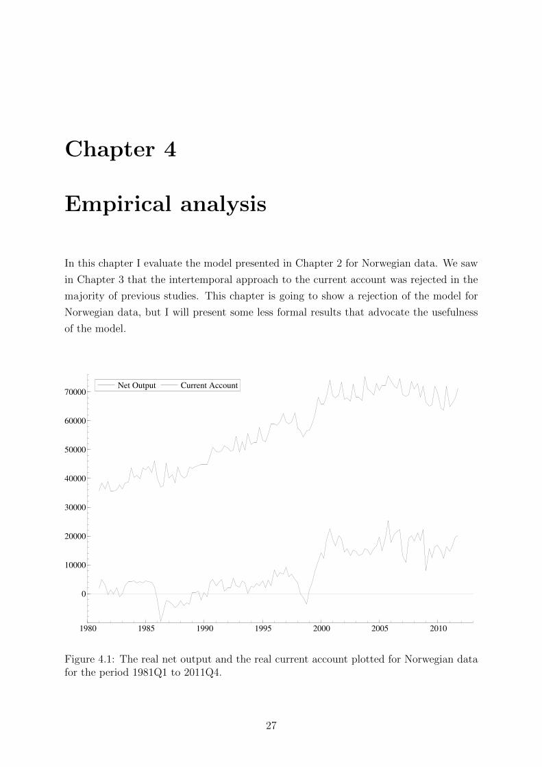
In this chapter I evaluate the model presented in Chapter 2 for Norwegian data. We saw
in Chapter 3 that the intertemporal approach to the current account was rejected in the
majority of previous studies. This chapter is going to show a rejection of the model for
Norwegian data, but I will present some less formal results that advocate the usefulness
of the model.
Net Output Current Account
1980 1985 1990 1995 2000 2005 2010
0
10000
20000
30000
40000
50000
60000
70000Net Output Current Account
Figure 4.1: The real net output and the real current account plotted for Norwegian datafor the period 1981Q1 to 2011Q4.
27
28 CHAPTER 4. EMPIRICAL ANALYSIS
4.1 Data
The variables of interest are gross domestic product, government spending, investment,
and the current account balance. I use quarterly data from 1981Q1 to 2011Q4, all data
used in this chapter is obtained from Statistics Norway.1 The data is deflated to real
and per-capita terms. The net output series is constructed by subtracting government
consumption and investment from the gross domestic product. The current account bal-
ance is equal to total export minus total import plus the balance of income and current
transfers. It is also worth noting that the data is not adjusted for seasonally fluctuations,
this is because I lack seasonally adjusted data for the current account series. I get some
significance for seasonal dummies in my regressions, but this will be ignored in the rest of
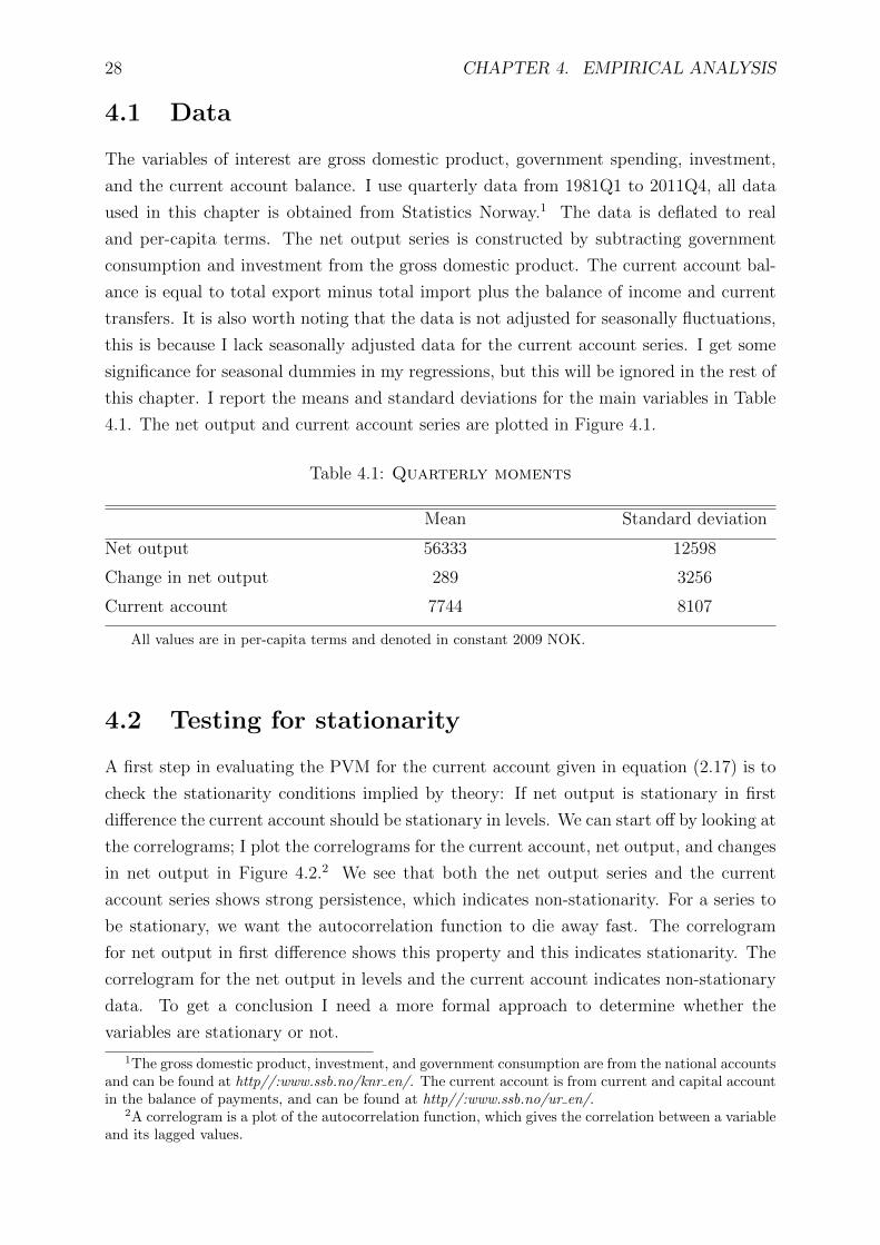
this chapter. I report the means and standard deviations for the main variables in Table
4.1. The net output and current account series are plotted in Figure 4.1.
Table 4.1: Quarterly moments
Mean Standard deviation
Net output 56333 12598
Change in net output 289 3256
Current account 7744 8107
All values are in per-capita terms and denoted in constant 2009 NOK.
4.2 Testing for stationarity
A first step in evaluating the PVM for the current account given in equation (2.17) is to
check the stationarity conditions implied by theory: If net output is stationary in first
difference the current account should be stationary in levels. We can start off by looking at
the correlograms; I plot the correlograms for the current account, net output, and changes
in net output in Figure 4.2.2 We see that both the net output series and the current
account series shows strong persistence, which indicates non-stationarity. For a series to
be stationary, we want the autocorrelation function to die away fast. The correlogram
for net output in first difference shows this property and this indicates stationarity. The
correlogram for the net output in levels and the current account indicates non-stationary
data. To get a conclusion I need a more formal approach to determine whether the
variables are stationary or not.
1The gross domestic product, investment, and government consumption are from the national accountsand can be found at http//:www.ssb.no/knr en/. The current account is from current and capital accountin the balance of payments, and can be found at http//:www.ssb.no/ur en/.
2A correlogram is a plot of the autocorrelation function, which gives the correlation between a variableand its lagged values.

4.2. TESTING FOR STATIONARITY 29
Current Account
1 2 3 4 5 6 7 8 9 10
0.5
1.0 Current Account
Change in Net Output
1 2 3 4 5 6 7 8 9 10
0
1Change in Net Output
Net Output
1 2 3 4 5 6 7 8 9 10
0.5
1.0 Net Output
Figure 4.2: Correlograms for net output, change in net output, and the current account.
A standard approach to test whether a time series is stationary is to use the augmented
Dickey-Fuller (ADF) test.3 The Dickey-Fuller test investigates whether a series is reverting
back to a mean. To perform the test we run a regression of the form
∆Xt = constant + φXt−1 +
q∑i=1
γi∆Xt−i + ηt, (4.1)
where Xt is the variable of interest and, φ and the γi’s are the parameters to be estimated.
The operator ∆ is defined as standard backward difference. The null-hypothesis is a unit
root in the time series Xt, and can be formulated as H0: φ = 0. If the time series has a
unit root the series is non-stationary. The alternative-hypothesis of no unit root is HA:
φ < 0. The test is performed as a t-test on φ, but with a different distribution of the
critical values. An important practical issue is how to choose the lag length q in equation
(4.1). If q is too low, the remaining serial correlation in the residuals can bias the test.
A too high q and the degrees of freedom will be low and the power of the test will suffer.
To determine q I apply the Akaike information criterion.4
The results from a unit root test for NOt, CAt, and ∆NOt are reported in Table 4.2.
For the ADF test for a unit root in net output the Akaike information criterion suggests
3See Dickey and Fuller (1979).4See section 4.4 for details on lag-selection using information criterion.

30 CHAPTER 4. EMPIRICAL ANALYSIS
Table 4.2: Unit root test for the period 1981–2011
NOt CAt ∆NOt
-0.02 -0.05 -1.36
(-1.3) (-1.3) (-4.1)
The reported parameter is φ. The sample size is 124. The number of lags is 11 in the test of NOt, 1in the test of CAt, and 7 in the test for ∆NOt. t-values in parentheses.
a lag length of 11. The computed ADF test statistic (-1.3) is higher than the 5 percent
critical value (-2.9), and we cannot reject the null-hypothesis of a unit root in net output,
net output is non-stationary as expected. For the stationarity test of ∆NOt, Akaike
suggests a lag length of 7, the ADF test statistic (-4.1) is below the 5 percent critical
value (-2.9) and we can reject the hypothesis of a unit root in ∆NOt, and the change
in net output is stationary. For the current account balance, the Akaike information
criterion suggests a lag length of 1. The computed ADF test statistic (-1.3) is higher than
the 5 percent critical value (-2.9) and we cannot reject the hypothesis of a unit root in
CAt. This is not in line with what we expected based on the intertemporal model in the
previous section. This is a crucial problem; the model and the statistical tests are not
valid if the current account series is non-stationary in levels.
However, the finding of a non-stationary current account is common in the literature
when standard Dickey-Fuller tests are applied; in Sheffrin and Woo (1990) the hypothesis
of a unit root in the current account cannot be rejected for any of the countries they
study. This problem is addressed in detail in a paper by Wu (2000): He finds support
for a stationary current account balance for industrialized countries even when standard
tests reject stationarity. The rest of this analysis is based on the assumption of a stable
current account balance.
4.3 The VAR and the PVM
To test the PVM given in equation (2.17), I follow the method developed by Campbell
(1987) and Campbell and Shiller (1987). The PVM for the current account is a nested
version of a general VAR. Campbell and Shiller show how to test PVMs by testing a set
of restrictions on a general VAR. I will show how to derive the PVM from a VAR. I start
off by finding an estimate for the representative consumer’s forecast of the change in net
output. To do this I treat conditional expectations as linear projections on information.
This means that the model for forecasting the current account and changes in net output
is a linear function of available information about the past. The information set I use is
previous values of the current account and previous changes in net output. The VAR is
set up with current dated variables of CAt and ∆NOt on the left-hand side, and lagged
4.3. THE VAR AND THE PVM 31
variables on the right-hand side. In general the system can be formulated as
∆NOt = α11∆NOt−1 + · · ·+ α1p∆NOt−p + β11CAt−1 + · · ·+ β1pCAt−p + ε1t
(4.2)
CAt = α21∆NOt−1 + · · ·+ α2p∆NOt−p + β21CAt−1 + · · ·+ β2pCAt−p + ε2t,
where the α’s and the β’s are parameters to be estimated, ε1t and ε2t are white noise
disturbance terms, and p is the number of lagged variables.5 There are no constant terms
in the system; this is because the data I use in the VAR is demeaned. The PVM is not
saying anything about the mean values of the variables, only the dynamic relationship
between them, so using demeaned values does not seem to affect the results in this analysis.
A matrix formulation of the system given in (4.2) can be obtained if we define
zt ≡
[∆NOt
CAt
], Ap ≡
[α1p β1p
α2p β2p
]and νt ≡
[ε1t
ε2t
],
then the VAR(p) can be written more compactly as
zt = A1zt−1 + A2zt−2 + · · ·+ Apzt−p + νt. (4.3)
To find a forecast for the change in net output, it is more convenient to work with a model
with only one lagged variable. It is possible to rewrite the VAR(p) in equation (4.3) as a
VAR(1) if we define
Ψt ≡
zt
zt−1
zt−2
...
zt−p+1
, Γ ≡
A1 A2 · · · Ap
I2 0 · · · 0
0 I2 · · · 0...
.... . .
...
0 · · · I2 0
and ξt ≡
νt
0
0...
0
.
The subscript on the identity matrix I indicates the matrix dimensions, so I2 is a (2× 2)
matrix. Let T be the number of observations and R the set of real numbers, then Ψt, ξt ∈R2p×T and Γ ∈ R2p×2p. The bold zeros represent matrices of zeros. The matrix Γ is called
the companion matrix of the VAR. Then, equation (4.3) can be written as a VAR(1)
Ψt = ΓΨt−1 + ξt. (4.4)
5A process is called white noise if the mean is zero, the variance is constant and the covariance’sbetween the terms are zero; see Hamilton (1994), Chapter 3. If the residuals satisfy the CLR assumptionspresented in Chapter 3 in this thesis, they are white noise.
32 CHAPTER 4. EMPIRICAL ANALYSIS
I use the regression model in equation (4.4) to make forecasts of future changes in net
output. If the VAR is stationary we can iterate backwards to get the following expression
for the expected value of Ψs
E[Ψs|Ωt] = Γs−tΨt, (4.5)
where Ωt is the representative consumer’s information set at time t.6,7 This information
set includes more information than what is directly observable to the econometrician.
The model predicts a current account balance that reflects the representative consumer’s
expectations about future changes in net output. If we include the current account in
the estimate for changes in net output, all the information available to the consumer is
used in our forecast of changes in net output. This is a strength of the Campbell-Shiller
procedure, and at least in theory, omitted information is not a problem when applying
this method. If we use equation (4.5), an expression for the representative consumer’s
forecast of future changes in output can be written as E[∆NOs|Ωt] = e∆NOΓs−tΨt, where
e∆NO ≡ [1 0 0 · · · 0] is a (1 × 2p) row vector constructed so that e∆NOΨt = ∆NOt.
If we use the expected value of the change in net output from the VAR in the PVM in
equation (2.17) we get
CAt = −∞∑
s=t+1
(1
1 + r
)s−te∆NOΓs−tΨt.
I define the real discount rate as τ ≡ 1/(1 + r). Contingent on a stationary VAR, the
model for the current account can be written as8
CAt = −e∆NO(τΓ)(I− τΓ)−1Ψt. (4.6)
I omit the subscript on the identity matrix and let I = I2p. To find the formal restrictions,
write eCAΨt = −e∆NO(τΓ)(I− τΓ)−1Ψt, where eCA ≡ [0 1 0 · · · 0] is a (1× 2p) row
vector, constructed so that eCAΨt = CAt. The model imply the following restriction on
the companion matrix from the VAR
eCA = −e∆NO(τΓ)(I− τΓ)−1. (4.7)
The next step is to estimate the parameter matrix Γ and find Γ. When Γ is determined
the restriction in equation (4.7) can be formally tested.
6The VAR is stationary if all the roots of the equation det(I − A1x − A2x2 − · · · − Apx
p) = 0 lieoutside the unit circle, see Appendix D.
7I use E[Ψs|Ωt] = E[(ΓΨs−1 + ξs)|Ωt] = ΓE[Ψs−1|Ωt] + E[ξs|Ωt] = Γ2E[Ψs−2|Ωt] = . . . , becauseξt is white noise where E[ξs|Ωt] = 0 for all s > t.
8
Because∞∑
s=t+1
τs−tΓs−t = τΓ[I + (τΓ) + (τΓ)2 + (τΓ)3 + . . .
]= (τΓ)(I− τΓ)−1.
4.4. DECIDING THE LAG LENGTH FOR THE VAR 33
4.4 Deciding the lag length for the VAR
The results from estimating a VAR depends on the lag length, so p needs to be decided.
A standard approach to discriminate between models of different lag lengths is to use
information criterion. To evaluate a model with information criterion, we must calculate
the following expression
Sp = log det(Σξ) + pg(T ), where Σξ =ξt · ξ
′t
T∈ R2p×2p
is the estimated variance-covariance matrix from the VAR and ξt is the estimated residual
values from the VAR in equation (4.4) given by ξt = Ψt − ΓΨt−1.9 The first term
log det(Σξ) is a measure of the fit of the model, where det(Σξ) is the determinant of the
matrix Σξ. The lower this value is the more accurate is the model in explaining the actual
data. We prefer a parsimonious model, so the second term pg(T ) is a penalty term for
including many parameters in the model. When using information criterion, the optimal
lag length is the solution to the following problem
p = arg minpSp.
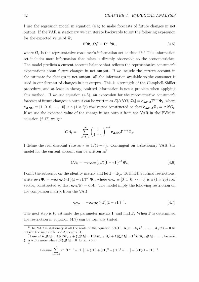
Table 4.3 reports information criterion for different lag lengths and different forms of
g(T ).10 We can see that the three specifications in Table 4.3 favors a lag length of p = 4.
Table 4.3: Lag selection in the VAR
p = 1 p = 2 p = 3 p = 4 p = 5 p = 6 p = 8 p = 10 p = 12
Akaike 32.03 31.73 31.14 30.77 30.80 30.78 30.85 30.86 30.92
Schwartz 32.13 31.91 31.42 31.15 31.27 31.34 31.62 31.83 32.09
Hannan-Quinn 31.07 31.80 31.26 30.93 31.00 31.01 31.17 31.26 31.39
All specifications of the information criterion prefer a lag length of 4.
4.5 Results from a general VAR(4)
A VAR where all right-hand side variables are exogenous can be estimated equation by
equation using ordinary least squares.9 The next step is to estimate the parameters in
the general VAR given in equation (4.4). Using matrix notation, the parameters are
calculated in the following way
ΓOLS = (Ψt−1 ·Ψ′t−1)−1
Ψt−1 ·Ψ′t.9See Hayashi (2000), Chapter 6.
10Akaike: g(T ) = 2/T , Schwartz: g(T ) = log T/T , and Hannan-Quinn: g(T ) = 2 log(log T )/T .
34 CHAPTER 4. EMPIRICAL ANALYSIS
Table 4.4: Results from the VAR(4)
∆NOt−1 ∆NOt−2 ∆NOt−3 ∆NOt−4
∆NOt -0.71 -0.65 -0.54 0.26(-6.5)[-6.5] (-5.3)[-4.9] (-5.0)[-4.6] (2.9)[3.0]
CAt 0.31 0.20 0.28 0.30(1.9)[1.9] (1.0)[1.0] (1.7)[1.5] (2.2)[1.8]
CAt−1 CAt−2 CAt−3 CAt−4
∆NOt 0.34 -0.01 -0.16 -0.24(4.2)[4.3] (-0.2)[-0.2] (-2.0)[-2.1] (-2.8)[-2.5]
CAt 0.54 0.21 0.01 0.22(4.5)[3.6] (1.7)[1.8] (0.0)[0.0] (1.8)[1.5]
The number of observations is 119, the number of lags is 4, t-values in parentheses, andheteroskedasticity-consistent t-values in brackets. The formula for calculating heteroskedastic ro-bust variances is given in equation (4.12).
Current Account Fitted
1985 1990 1995 2000 2005 2010
−10000
0
10000
Current Account Fitted
Change in Net Output Fitted
1985 1990 1995 2000 2005 2010
−5000
0
5000
Change in Net Output Fitted
Figure 4.3: Actual values plotted against the fitted values from the unrestricted VAR(4)
for the sample period 1982Q2 to 2011Q4.
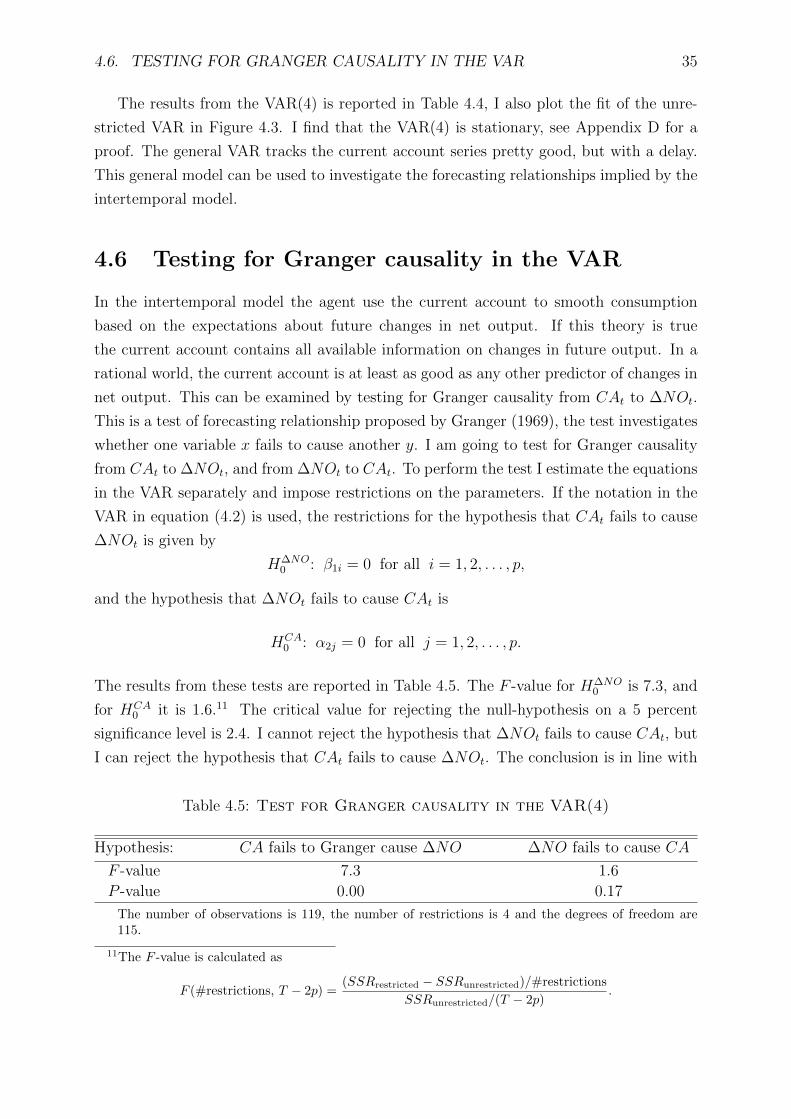
4.6. TESTING FOR GRANGER CAUSALITY IN THE VAR 35
The results from the VAR(4) is reported in Table 4.4, I also plot the fit of the unre-
stricted VAR in Figure 4.3. I find that the VAR(4) is stationary, see Appendix D for a
proof. The general VAR tracks the current account series pretty good, but with a delay.
This general model can be used to investigate the forecasting relationships implied by the
intertemporal model.
4.6 Testing for Granger causality in the VAR
In the intertemporal model the agent use the current account to smooth consumption
based on the expectations about future changes in net output. If this theory is true
the current account contains all available information on changes in future output. In a
rational world, the current account is at least as good as any other predictor of changes in
net output. This can be examined by testing for Granger causality from CAt to ∆NOt.
This is a test of forecasting relationship proposed by Granger (1969), the test investigates
whether one variable x fails to cause another y. I am going to test for Granger causality
from CAt to ∆NOt, and from ∆NOt to CAt. To perform the test I estimate the equations
in the VAR separately and impose restrictions on the parameters. If the notation in the
VAR in equation (4.2) is used, the restrictions for the hypothesis that CAt fails to cause
∆NOt is given by
H∆NO0 : β1i = 0 for all i = 1, 2, . . . , p,
and the hypothesis that ∆NOt fails to cause CAt is
HCA0 : α2j = 0 for all j = 1, 2, . . . , p.
The results from these tests are reported in Table 4.5. The F -value for H∆NO0 is 7.3, and
for HCA0 it is 1.6.11 The critical value for rejecting the null-hypothesis on a 5 percent
significance level is 2.4. I cannot reject the hypothesis that ∆NOt fails to cause CAt, but
I can reject the hypothesis that CAt fails to cause ∆NOt. The conclusion is in line with
Table 4.5: Test for Granger causality in the VAR(4)
Hypothesis: CA fails to Granger cause ∆NO ∆NO fails to cause CA
F -value 7.3 1.6
P -value 0.00 0.17
The number of observations is 119, the number of restrictions is 4 and the degrees of freedom are115.
11The F -value is calculated as
F (#restrictions, T − 2p) =(SSRrestricted − SSRunrestricted)/#restrictions
SSRunrestricted/(T − 2p).

36 CHAPTER 4. EMPIRICAL ANALYSIS
what the theory predicts; the data indicates a forecasting relationship from the current
account to changes in net output, so the current account is useful in predicting changes
in net output. We do not see causality the other way, past changes in net output is not
useful in predicting the current account.
4.7 Testing the PVM
I have the estimated parameter matrix Γ and can use equation (4.6) to find the predicted
current account from the intertemporal model; the predicted current account series is
given by
CAt = −e∆NO(τ Γ)(I− τ Γ)−1Ψt.
It is important to distinguish between CAt, CAt and CAt, the first CAt is the actual
current account, CAt is the fitted current account from the VAR and CAt is the predicted
current account from the PVM. If the theory holds, the actual and predicted current
account should be equal, that is CAt = CAt. We can look at this graphically by plotting
the predicted values against the actual series. This is done in Figure 4.4. In this plot the
annual world real interest rate is assumed to be 4 percent, which corresponds to r = 0.01.
Actual Current Account Predicted Current Account
1985 1990 1995 2000 2005 2010
−15000
−10000
−5000
0
5000
10000
15000
Actual Current Account Predicted Current Account
Figure 4.4: Actual current account plotted against predicted current account from 1982Q2to 2011Q4 where the predicted values are from the intertemporal model.

4.7. TESTING THE PVM 37
As we can see, the predicted series tracks the actual series pretty good, the correlation
between the actual and predicted current account is 0.97. Obstfeld and Rogoff (1996
pp. 93-95), plots similar results for different countries and state that the nice graphical
results are surprising given the simplicity of the model. So at least the graphical results
advocate the usefulness of the intertemporal approach for explaining Norwegian data. An
even stronger statement is in Otto (1992 pp. 421) where he writes: “. . . if CAt tracks CAt
closely, then a statistical rejection of the model may be of little economic importance.”
Note that CAt in this sentence is equal to CAt in my notation.
Another implication is that the variance of the actual and predicted current account
should be equal. In my findings the actual series is more volatile than the predicted
series. The ratio of the variance for the predicted series over the variance for the actual
series is 0.75, so the model predicts less consumption smoothing than what we observe in
the data. This indicates that net capital flow from Norway has been more volatile than
what we can expect based on what is necessary for consumption smoothing. At least
capital mobility has not been too limited for Norway. In the literature this is called excess
volatility, which means that the consumption-smoothing component of foreign lending is
more volatile than what we expect based on the permanent income theory.12
To test whether CAt and CAt are statistical different, I need to test the restrictions
that give the predicted series CAt. To find the specific restrictions on the parameters in
the VAR, we can look back to the formal restriction on the parameter matrix Γ given by
equation (4.7)
eCA = −e∆NO(τΓ)(I− τΓ)−1.
If the matrix (I − τΓ)−1 is invertible it is possible to calculate linear cross-equation
restrictions on the parameters in the VAR. If we solve eCA(I− τΓ) = −e∆NO(τΓ) for the
parameters, we get the following restrictions
α1i = α2i for i = 1, 2, . . . , p, β1j = β2j for j = 2, 3, . . . , p, and τβ21 = 1 + τβ11, (4.8)
see Appendix C for details on the calculation of the restrictions. It is also possible to
calculate non-linear restrictions on the parameters that satisfy equation (4.7). To find the
non-linear restrictions we need to solve the matrix (I−τΓ)−1 for the parameters; this will
get algebraically messy and I will not pursue these non-linear restrictions in this thesis.
One way to test the validity of the restrictions is to estimate the restricted VAR and
compare the general and the restricted VAR and check whether the models are statistically
different; this is the log-likelihood ratio test presented bellow. The estimation procedure
for a restricted VAR is usually maximum likelihood (ML). I will not go into the details
on the ML estimation method.13 The results from the estimation of the restricted VAR
12See examples of excess volatility in Sheffrin and Woo (1990), Ghosh (1995), and Agenor et al. (1999).13See e.g. Hamilton (1994), Chapter 11.

38 CHAPTER 4. EMPIRICAL ANALYSIS
are from the software package OxMetrics. The estimated restricted VAR(4) is given by
∆NOt = − 0.73∆NOt−1 − 0.67∆NOt−2 − 0.57∆NOt−3 + 0.30NOt−4
+ 0.36CAt−1 − 0.02CAt−2 − 0.16CAt−3 − 0.25CAt−4
CAt = − 0.73∆NOt−1 − 0.67∆NOt−2 − 0.57∆NOt−3 + 0.30∆NOt−4
+ 1.36CAt−1 − 0.02CAt−2 − 0.16CAt−3 − 0.25CAt−4
I plot the model for the current account where the linear restrictions are imposed in Figure
4.5.
Current Account Fitted
1985 1990 1995 2000 2005 2010
−10000
0
10000
Current Account Fitted
Change in Net Output Fitted
1985 1990 1995 2000 2005 2010
−5000
0
5000
Change in Net Output Fitted
Figure 4.5: The predicted values from the restricted VAR(4) plotted against the actualvalues for the sample period 1982Q2 to 2011Q4. The restrictions are linear.
For the intertemporal model to be statistical valid, we must be able to confirm that
the restrictive VAR presented in Figure 4.5 is a valid simplification of the general VAR
presented in Figure 4.3. There are different ways of testing the restrictive VAR against
the general VAR. I will present a Wald test, a log-likelihood ratio test, and a Lagrange
multiplier test, and as noted in Chapter 3 they are all asymptotically equal. The Wald
test and the Lagrange-multiplier test can be performed without estimating the restricted
VAR. I present the Wald test after the residual analysis in section 4.9 because the Wald
test can easily be made robust to heteroskedasticity, which we will see may be a problem.
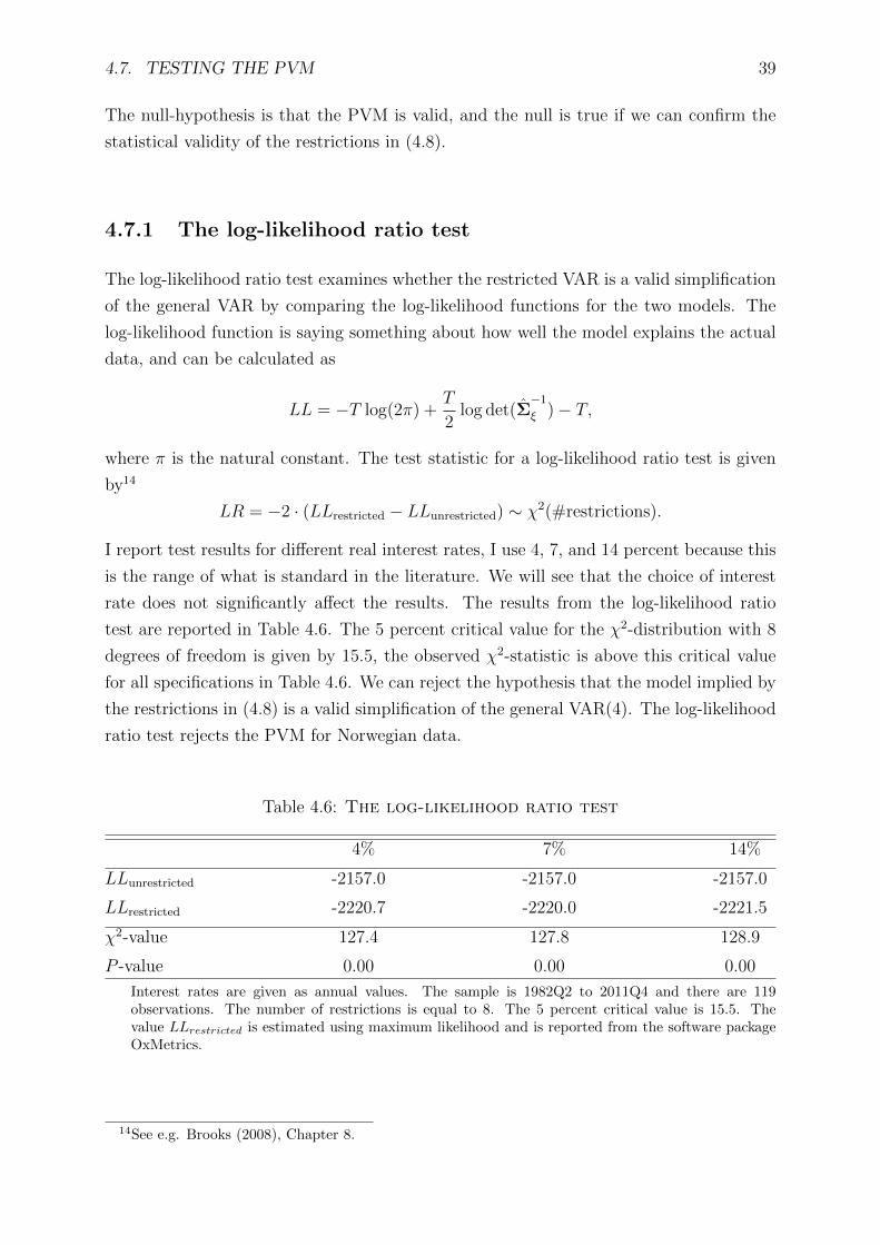
4.7. TESTING THE PVM 39
The null-hypothesis is that the PVM is valid, and the null is true if we can confirm the
statistical validity of the restrictions in (4.8).
4.7.1 The log-likelihood ratio test
The log-likelihood ratio test examines whether the restricted VAR is a valid simplification
of the general VAR by comparing the log-likelihood functions for the two models. The
log-likelihood function is saying something about how well the model explains the actual
data, and can be calculated as
LL = −T log(2π) +T
2log det(Σ
−1
ξ )− T,
where π is the natural constant. The test statistic for a log-likelihood ratio test is given
by14
LR = −2 · (LLrestricted − LLunrestricted) ∼ χ2(#restrictions).
I report test results for different real interest rates, I use 4, 7, and 14 percent because this
is the range of what is standard in the literature. We will see that the choice of interest
rate does not significantly affect the results. The results from the log-likelihood ratio
test are reported in Table 4.6. The 5 percent critical value for the χ2-distribution with 8
degrees of freedom is given by 15.5, the observed χ2-statistic is above this critical value
for all specifications in Table 4.6. We can reject the hypothesis that the model implied by
the restrictions in (4.8) is a valid simplification of the general VAR(4). The log-likelihood
ratio test rejects the PVM for Norwegian data.
Table 4.6: The log-likelihood ratio test
4% 7% 14%
LLunrestricted -2157.0 -2157.0 -2157.0
LLrestricted -2220.7 -2220.0 -2221.5
χ2-value 127.4 127.8 128.9
P -value 0.00 0.00 0.00
Interest rates are given as annual values. The sample is 1982Q2 to 2011Q4 and there are 119observations. The number of restrictions is equal to 8. The 5 percent critical value is 15.5. Thevalue LLrestricted is estimated using maximum likelihood and is reported from the software packageOxMetrics.
14See e.g. Brooks (2008), Chapter 8.
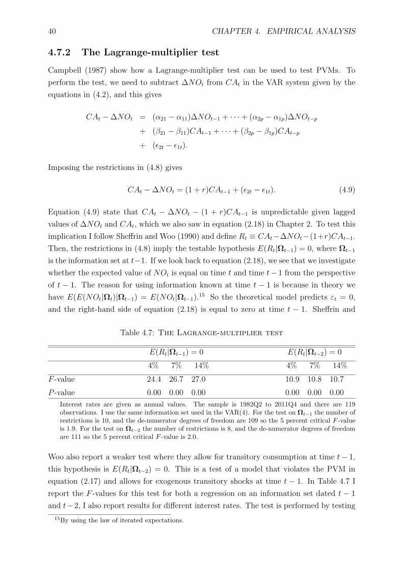
40 CHAPTER 4. EMPIRICAL ANALYSIS
4.7.2 The Lagrange-multiplier test
Campbell (1987) show how a Lagrange-multiplier test can be used to test PVMs. To
perform the test, we need to subtract ∆NOt from CAt in the VAR system given by the
equations in (4.2), and this gives
CAt −∆NOt = (α21 − α11)∆NOt−1 + · · ·+ (α2p − α1p)∆NOt−p
+ (β21 − β11)CAt−1 + · · ·+ (β2p − β1p)CAt−p
+ (ε2t − ε1t).
Imposing the restrictions in (4.8) gives
CAt −∆NOt = (1 + r)CAt−1 + (ε2t − ε1t). (4.9)
Equation (4.9) state that CAt − ∆NOt − (1 + r)CAt−1 is unpredictable given lagged
values of ∆NOt and CAt, which we also saw in equation (2.18) in Chapter 2. To test this
implication I follow Sheffrin and Woo (1990) and define Rt ≡ CAt−∆NOt−(1+r)CAt−1.
Then, the restrictions in (4.8) imply the testable hypothesis E(Rt|Ωt−1) = 0, where Ωt−1
is the information set at t−1. If we look back to equation (2.18), we see that we investigate
whether the expected value of NOt is equal on time t and time t− 1 from the perspective
of t − 1. The reason for using information known at time t − 1 is because in theory we
have E(E(NOt|Ωt)|Ωt−1) = E(NOt|Ωt−1).15 So the theoretical model predicts εt = 0,
and the right-hand side of equation (2.18) is equal to zero at time t − 1. Sheffrin and
Table 4.7: The Lagrange-multiplier test
E(Rt|Ωt−1) = 0 E(Rt|Ωt−2) = 0
4% 7% 14% 4% 7% 14%
F -value 24.4 26.7 27.0 10.9 10.8 10.7
P -value 0.00 0.00 0.00 0.00 0.00 0.00
Interest rates are given as annual values. The sample is 1982Q2 to 2011Q4 and there are 119observations. I use the same information set used in the VAR(4). For the test on Ωt−1 the number ofrestrictions is 10, and the de-numerator degrees of freedom are 109 so the 5 percent critical F -valueis 1.9. For the test on Ωt−2 the number of restrictions is 8, and the de-numerator degrees of freedomare 111 so the 5 percent critical F -value is 2.0.
Woo also report a weaker test where they allow for transitory consumption at time t− 1,
this hypothesis is E(Rt|Ωt−2) = 0. This is a test of a model that violates the PVM in
equation (2.17) and allows for exogenous transitory shocks at time t − 1. In Table 4.7 I
report the F -values for this test for both a regression on an information set dated t − 1
and t−2, I also report results for different interest rates. The test is performed by testing
15By using the law of iterated expectations.
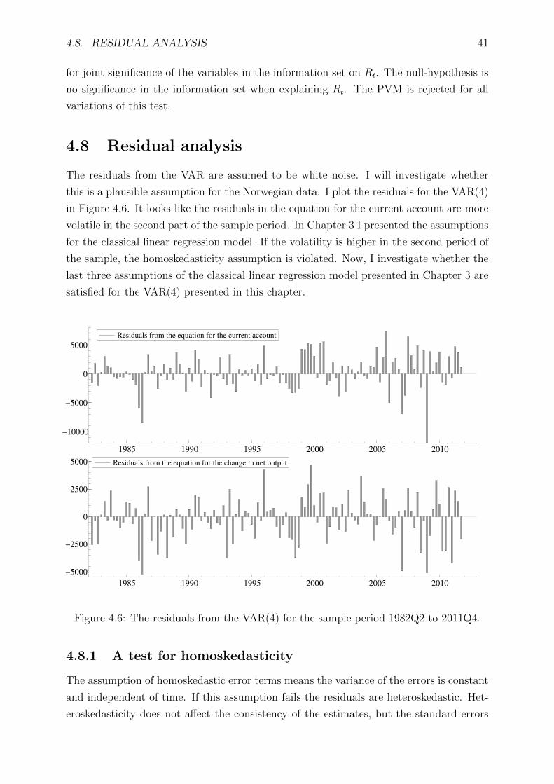
4.8. RESIDUAL ANALYSIS 41
for joint significance of the variables in the information set on Rt. The null-hypothesis is
no significance in the information set when explaining Rt. The PVM is rejected for all
variations of this test.
4.8 Residual analysis
The residuals from the VAR are assumed to be white noise. I will investigate whether
this is a plausible assumption for the Norwegian data. I plot the residuals for the VAR(4)
in Figure 4.6. It looks like the residuals in the equation for the current account are more
volatile in the second part of the sample period. In Chapter 3 I presented the assumptions
for the classical linear regression model. If the volatility is higher in the second period of
the sample, the homoskedasticity assumption is violated. Now, I investigate whether the
last three assumptions of the classical linear regression model presented in Chapter 3 are
satisfied for the VAR(4) presented in this chapter.
Residuals from the equation for the current account
1985 1990 1995 2000 2005 2010
−10000
−5000
0
5000
Residuals from the equation for the current account
Residuals from the equation for the change in net output
1985 1990 1995 2000 2005 2010
−5000
−2500
0
2500
5000 Residuals from the equation for the change in net output
Figure 4.6: The residuals from the VAR(4) for the sample period 1982Q2 to 2011Q4.
4.8.1 A test for homoskedasticity
The assumption of homoskedastic error terms means the variance of the errors is constant
and independent of time. If this assumption fails the residuals are heteroskedastic. Het-
eroskedasticity does not affect the consistency of the estimates, but the standard errors

42 CHAPTER 4. EMPIRICAL ANALYSIS
are incorrect and standard testing procedures such as t- and F -tests are invalid. I will
now test whether the residuals plotted in Figure 4.6 are homoskedastic as assumed. A
popular test for heteroskedasticity is the White test.16 This test can be performed by re-
gressing the squared residual values on the explanatory variables and squared explanatory
variables. The equations to be estimated are given by
ε21t = δ0 + δ1CAt−1 + δ2CAt−2 + δ3CAt−3 + δ4CAt−4 + δ5∆NOt−1
+δ6∆NOt−2 + δ7∆NOt−3 + δ8∆NOt−4 + δ9CA2t−1 + δ10CA
2t−2
+δ11CA2t−3 + δ12CA
2t−4 + δ13∆NO2
t−1 + δ14∆NO2t−2 + δ15∆NO2
t−3
+δ16∆NO2t−4 + error
ε22t = δ17 + δ18CAt−1 + δ19CAt−2 + δ20CAt−3 + δ21CAt−4 + δ22∆NOt−1
+δ23∆NOt−2 + δ24∆NOt−3 + δ25∆NOt−4 + δ26CA2t−1 + δ27CA
2t−2
+δ28CA2t−3 + δ29CA
2t−4 + δ30∆NO2
t−1 + δ31∆NO2t−2 + δ32∆NO2
t−3
+δ33∆NO2t−4 + error,
where ε1t and ε2t is the estimated residuals from the VAR(4). The null-hypothesis is
homoskedasticity and this is the case for both equations if we can confirm statistically
that all the δ’s except δ0 and δ17 are equal to zero. The test can also include cross-terms
of the regressors; results with and without cross-terms are reported in Table 4.8. The
results indicate heteroskedastic residuals in the equation for the current account. For
the equation for the change in net output we observe mixed results; we cannot reject
homoskedasticity in the specification without cross terms, but the null-hypothesis can be
rejected on a 5 percent significance level in the specification with cross-terms. It looks
like we may have a problem with heteroskedasticity in both equations.
Table 4.8: Testing for homoskedasticity
Test without cross-terms Equation for ∆NOt Equation for CAt
F -value 1.4 1.8
P -value 0.15 0.04Test with cross-terms Equation for ∆NOt Equation for CAt
F -value 1.6 2.5
P -value 0.04 0.00
The sample is 1982Q2 to 2011Q4 and there are 119 observations. The test without cross-terms has16 restrictions and the degrees of freedom are 102, the test with cross-terms has 44 restrictions andthe degrees of freedom are 74.
16See White (1980).

4.8. RESIDUAL ANALYSIS 43
4.8.2 A test for serial correlation
The assumption of no serial correlation means that all the residuals need to be independent
of one another, and we should not see any correlation between residuals. The presence of
serial correlation may indicate a misspecified model. I will test for serial correlation using
the Breusch-Godfrey test.17 This test is performed by regressing the residual values on
the explanatory variables and lagged values of the residuals; the regression equations are
given by
ε1t = δ0 + δ1CAt−1 + δ2CAt−2 + δ3CAt−3 + δ4CAt−4 + δ5∆NOt−1
+δ6∆NOt−2 + δ7∆NOt−3 + δ8∆NOt−4 + δ9ε1t−1 + δ10ε1t−2
+δ11ε1t−3 + δ12ε1t−4 + δ13ε1t−5 + error
ε1t = δ14 + δ15CAt−1 + δ16CAt−2 + δ17CAt−3 + δ18CAt−4 + δ19∆NOt−1
+δ20∆NOt−2 + δ21∆NOt−3 + δ22∆NOt−4 + δ23ε2t−1 + δ24ε2t−2
+δ25ε2t−3 + δ26ε2t−4 + δ27ε2t−5 + error.
The null-hypothesis is no serial correlation, and can be formally tested by saving the R2
from the regressions of ε1t and ε2t and calculating the following test statistic
BG = (T − 5)R2 ∼ χ2(5).
The results from this test are reported in Table 4.9. The null-hypothesis of no serial
correlation cannot be rejected for any of the equations on the 5 percent significance level.
Based on the Breusch-Godfrey test for normality, I can conclude that the assumption of
no autocorrelation is satisfied in the VAR(4).
Table 4.9: Testing for serial correlation
Equation for ∆NOt Equation for CAt
χ2-value 6.1 9.7
P -value 0.29 0.08
The sample is 1983Q3 to 2011Q4 and there are 114 observations. The degrees of freedom are 5.
17See Breusch (1978) and Godfrey (1978).

44 CHAPTER 4. EMPIRICAL ANALYSIS
4.8.3 A test for normality
Normality is a property of the underlying distribution of a variable. If the normality
assumption is violated the statistical tests are invalid. For the normality test I use the
Jarque-Bera test, which has the following test statistic
JB =T
6
(Sk(εt)
2 +1
4(Ku(εt)− 3)2
)∼ χ2(2),
where Sk(εt) is the skewness and Ku(εt) is the kurtosis for the sample residuals.18 The
skewness and kurtosis is defined as
Sk(εt) ≡1/T
T∑t=1
(εt − ¯ε)3
(1/T
T∑t=1
(εt − ¯ε)2
)3/2and Ku(εt) ≡
1/TT∑t=1
(εt − ¯ε)4(1/T
T∑t=1
(εt − ¯ε)2
)2 ,
where ¯ε is the average value of the estimated residuals. The null-hypothesis is a normal
distribution. If the sample has a normal distribution, we expect the skewness to be 0
and the kurtosis to be 3. If the data deviates from these properties, the JB-statistic will
increase and the null-hypothesis gets less probable. The results from this test can be
found in Table 4.10. We see the null is rejected for the equation for the current account
while it cannot be rejected for the equation for changes in net output. Based on this
investigation, I conclude that ε1t has a normal distribution while ε2t does not.
Table 4.10: Testing for normality
Equation for ∆NOt Equation for CAt
Sk(εt) -0.23 -0.60
Ku(εt) 3.00 4.94χ2-value 1.1 25.8
P -value 0.59 0.00
The sample is 1982Q2 to 2011Q4 and there are 119 observations. The degrees of freedom are 2.
From the residual analysis we see that the model has a problem with both heteroskedas-
tic residuals and residuals that are not normally distributed. I will not address the nor-
mality problem. In the next section I present a heteroskedastic robust test of the PVM.
18See Jarque and Bera (1987).

4.9. THE WALD TEST 45
4.9 The Wald test
In this section I present the Wald test, I report the test for both the standard variance-
covariance matrix and for a heteroskedasticity robust variance-covariance matrix. Let us
again start off by the general restriction given by eCA = −e∆NO(τΓ)(I−τΓ)−1. If (I−τΓ)
is invertible we can calculate linear restrictions in the parameters, these restrictions are
given in (4.8), presented in matrix notation, they can be written as
eCA = τ(eCA − e∆NO)Γ.
To perform the linear Wald test I follow a paper by Bouakez and Kano (2009). First
define
I(Γ) ≡ eCA − τ(eCA − e∆NO)Γ ∈ R1×2p, (4.10)
then the null-hypothesis is given by I(Γ) = 0. By using the estimated parameters we can
calculate
τ(eCA − e∆NO)Γ = [1.01 0.20 0.85 0.22 0.81 0.16 0.04 0.46],
which should not be statistical different from the vector eCA = [0 1 0 · · · 0] for
the PVM to be confirmed. By visually comparing the two vectors, the results are not
convincing. I use the Wald test to check whether they are statistically different. The
Wald statistic is given by
W = I(Γ)
[∂I(Γ)
∂ΓΣΓ
∂I(Γ)
∂Γ′
]−1
I(Γ)′ ∼ χ2(#restrictions),
where ΣΓ is the estimated variance-covariance matrix for the parameter matrix, and
∂I(Γ)/∂Γ is the derivative of the matrix I(Γ) with respect to Γ evaluated at Γ. The
estimated variance-covariance matrix for the parameters can be calculated as
ΣΓ =T
T − 2pΣξ ⊗ (Ψt−1 ·Ψ′t−1)−1 =
ξt · ξt′
T − 2p⊗ (Ψt−1 ·Ψ′t−1)−1 ∈ R4p2×4p2 , (4.11)
where ⊗ is the Kronecker product.19,20 We also need the derivative of equation (4.10)
with respect to Γ, which is given by
∂I(Γ)
∂Γ= −τ(eCA − e∆NO)⊗ I2p ∈ R2p×4p2 .
19See Hayashi (2000), Chapter 6.20For details on how to calculate a Kronecker product see e.g. Graham (1981).
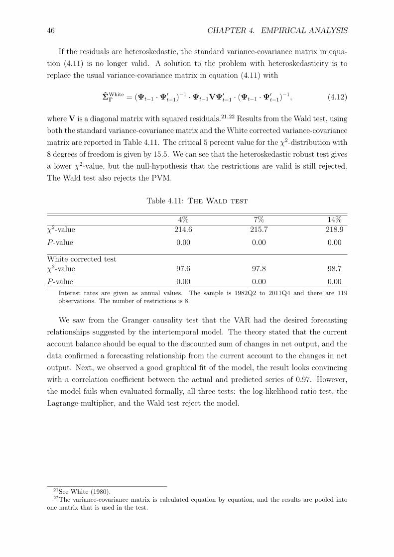
46 CHAPTER 4. EMPIRICAL ANALYSIS
If the residuals are heteroskedastic, the standard variance-covariance matrix in equa-
tion (4.11) is no longer valid. A solution to the problem with heteroskedasticity is to
replace the usual variance-covariance matrix in equation (4.11) with
ΣWhiteΓ = (Ψt−1 ·Ψ′t−1)−1 ·Ψt−1VΨ′t−1 · (Ψt−1 ·Ψ′t−1)−1, (4.12)
where V is a diagonal matrix with squared residuals.21,22 Results from the Wald test, using
both the standard variance-covariance matrix and the White corrected variance-covariance
matrix are reported in Table 4.11. The critical 5 percent value for the χ2-distribution with
8 degrees of freedom is given by 15.5. We can see that the heteroskedastic robust test gives
a lower χ2-value, but the null-hypothesis that the restrictions are valid is still rejected.
The Wald test also rejects the PVM.
Table 4.11: The Wald test
4% 7% 14%χ2-value 214.6 215.7 218.9
P -value 0.00 0.00 0.00
White corrected testχ2-value 97.6 97.8 98.7
P -value 0.00 0.00 0.00
Interest rates are given as annual values. The sample is 1982Q2 to 2011Q4 and there are 119observations. The number of restrictions is 8.
We saw from the Granger causality test that the VAR had the desired forecasting
relationships suggested by the intertemporal model. The theory stated that the current
account balance should be equal to the discounted sum of changes in net output, and the
data confirmed a forecasting relationship from the current account to the changes in net
output. Next, we observed a good graphical fit of the model, the result looks convincing
with a correlation coefficient between the actual and predicted series of 0.97. However,
the model fails when evaluated formally, all three tests: the log-likelihood ratio test, the
Lagrange-multiplier, and the Wald test reject the model.
21See White (1980).22The variance-covariance matrix is calculated equation by equation, and the results are pooled into
one matrix that is used in the test.

Chapter 5
A discussion of the rejection
As Chapter 4 shows, the theoretical model developed in Chapter 2 is rejected for Nor-
wegian data. In this chapter I will discuss the rejection of this simple version of the
intertemporal model. I will try to point out some possible problems of the model and
suggest possible improvements of the basic framework. Implementing these possible im-
provements in the theoretical model is beyond the scope of this thesis. I present a brief
review of some related papers that try to improve the basic model. I am also going to
estimate a general VAR for the current account and the change in net output where I will
include the unemployment rate and the price of oil as exogenous explanatory variables. I
will test whether these extra variables are helpful in explaining the current account and
the change in net output.
5.1 Possible causes for the rejection
The model in Chapter 2 makes many simplifying assumptions such as an exogenous supply
side, a one-good economy, and a single representative rational agent. Obviously these are
not realistic assumptions, but there are some good arguments for this approach. The
purpose of the economic model is to study a specific feature of the economy, which in this
thesis is a nation’s intertemporal wealth allocation. If we use a more complicated model
it may be harder to interpret the effects of this particular feature of the economy. The
model also needs to be simple enough so the theory can be tested against actual data.
The exogenous supply side assumption may be justified if the economy is small and
open so the production side does not affect prices. The single good can be thought of as an
index that represents an aggregate of all available goods. The model in my thesis lack the
choice between labor and leisure, it may be reasonable to think that some agents prefer
to increase leisure when the wealth increases. It may be relevant for the current account
how this leisure allocation is affecting the consumption and saving decision; this may be
solved by using a utility function that includes leisure. Next, I look at the rationality
assumption and the possibility that the agent dislikes risk.
47

48 CHAPTER 5. A DISCUSSION OF THE REJECTION
5.1.1 Rational agents
The rationality assumption carries a heavy load for the intertemporal model. It is assumed
that all agents behave symmetrically, and that one representative agent can model their
behavior. This agent has preferences that can be explained mathematically by a utility
function, and the agent make choices where the motive is to maximize the value of this
utility function. All the choices the agent makes are based on rational forward-looking
calculations where all publicly available information is used. It is worth noting that
rationality does not imply an agent that is always right about the future, but the mistakes
are random so the agent does not make systematic errors when predicting the future. We
can say the agent is right on average.
One possible break of the rationality assumption is dynamic inconsistency or present
bias, which means that the agent has a misperception about own time-preference. The
model in Chapter 2 assumes exponential discounting, which implies that events in the far
future are valued less than events that are close to the present, and the present is valued
the most. Present bias means that the agent’s preferences are changing over time, and
when the agent actually reach one of the future periods the agent realizes that the present
is valued more than what was expected in earlier periods. The effect from present bias
is that the agent consumes more every period than what was actually planned. When
consumption is higher than planned, saving is lower and consumption get tilted to the
present and we may see a lower current account surplus or even a deficit when we expect
a large surplus.
5.1.2 Uncertainty and precautionary saving
Another aspect of holding foreign assets that is ignored in the model presented in this
thesis is the motive for holding foreign assets as a way of insurance. In a world where future
outcomes are uncertain, it may be desirable for the agent to insure against unforeseen
events. If the agent is risk averse he or she may want to save more today than what we
can explain by consumption smoothing alone. This extra saving is called precautionary
saving. The current account will then consist of one intertemporal smoothing part and one
precautionary saving part. The reason why precautionary saving is ignored in the model
in this thesis is the assumption that the agent’s utility can be represented by a quadratic
function, a quadratic utility function makes the agent risk neutral and we get the result
of certainty equivalence when the agent is calculating the present value of permanent
income. Technically precautionary saving is a result of using a utility function where the
third derivative is positive.
Norway has large oil reserves and it is reasonable to think that this affects the country’s
choice on how much to save or borrow from the rest of the world. One factor is that the
oil industry is very capital intensive and has a high demand for investment in early stages

5.2. EXTENSIONS OF THE BASIC MODEL IN THE LITERATURE 49
of development. When the oil industry is starting up it may be an optimal strategy for
the country to borrow heavily to invest and repay this as the industry matures. When the
oil reserves are large they have a big impact on the nation’s wealth; uncertainties about
these reserves and the price of oil in the future may be important for the saving decision.
Uncertainties about both the size of unexplored reserves and the price of the oil in the
future may create incentives for significant levels of precautionary savings.
5.2 Extensions of the basic model in the literature
Several papers extend the basic model presented in Chapter 2. I give a brief review of
some of these attempts to improve the empirical fit of the intertemporal model. Bergin
and Sheffrin (2000) develop a model that allows for both traded and non-traded goods.
The paper presents a model that includes a variable interest rate and a variable exchange
rate. The model is tested for Canada, Australia, and the United Kingdom for the pe-
riod 1961 to 1996. They compare the model to a benchmark model similar to the one I
present in Chapter 2 and show an improved fit for Canada and Australia, but not for the
United Kingdom. Iscan (2002) extends the basic model to include durable and non-traded
goods; the model is tested for Canadian data for the period 1937 to 1994. The model
shows improvement when both durable and traded goods are included, but durable goods
alone do not improve the model. Ghosh and Ostry (1997) introduce a utility function
that makes the consumer risk averse. In this framework precautionary saving is present
and is an additional channel to the current account balance besides the intertemporal
smoothing motive. Their results suggest increased saving when the macroeconomic un-
certainty is heightened in the economy. If the current account is in surplus because of the
intertemporal smoothing motive, the precautionary saving motive will add to this surplus.
Nason and Rogers (2006) tries to find the parts of the PVM that is responsible for
the broad empirical rejection in the literature. They set up a small open economy real
business cycle model, which nests the PVM as a special case. In their framework they
investigate the impact of what they call the usual suspects for causing the PVM to fail.
These usual suspects are non-separable preferences, fiscal policy and real interest rate
shocks, external imperfect international capital mobility, and internalized risk premium.
When Nason and Rogers talk about the non-separability of the preferences, this is with
respect to consumption and leisure, the preferences are still time-separable. Fiscal policy
is modeled as demand shocks affecting the current account. Interest rate shocks affect
the return on savings. External imperfect capital mobility hinders the flow of capital
and make both saving and borrowing more difficult. Internalized risk premium is taking
up a point where in a small open economy the supply decision may affect the national
risk premium, and may therefore affect the decision on how much to save home and
abroad. Nason and Rogers confirm the rejection for Canadian data in a model without

50 CHAPTER 5. A DISCUSSION OF THE REJECTION
any suspects. To investigate the importance of the usual suspects they use a Bayesian
Monte Carlo experimental approach. They find an effect from all suspects, but the basic
model without any suspects performs best. However, the paper identifies the internalized
risk premium and exogenous world real interest rate shocks to be two important factors
for the rejection of the model.
5.3 An extended VAR
It may be interesting to see empirically how other factors affect the current account and the
change in net output. To do this I will estimate a VAR where I include the unemployment
rate and the price of oil as exogenous variables. I use quarterly data for the period 1987Q3
to 2011Q4. The unemployment rate is from the Organisation for Economic Co-operation
and Development (OECD).1 The oil price is the price of Brent Blend and is denoted in
real 2008 USD. The data for the price of oil is from Statistics Norway.2 The regression
model is given by the following two equations
CAt = constant+ α11CAt−1 + · · ·+ α1pCAt−p + β11∆NOt−1 + · · ·+ β1p∆NOt−p
+δ11POilt−1 + · · ·+ δ1pP
Oilt−p + γ11Ut−1 + · · ·+ γ1pUt−p + error (5.1)
∆NOt = constant+ α21CAt−1 + · · ·+ α2pCAt−p + β21∆NOt−1 + · · ·+ β2p∆NOt−p
+δ21POilt−1 + · · ·+ δ2pP
Oilt−p + γ21Ut−1 + · · ·+ γ2pUt−p + error (5.2)
where Ut is the unemployment rate in percent and POilt is the price of oil. In this section
the data is not demeaned so I include a constant. The Akaike information criterion suggest
a lag length of 5, and I present the results for the VAR(5) in Table 5.1. The model is
plotted in Figure 5.1. I will test whether POil and U are significant explanatory variables.
I test the null-hypothesis that none of the new variables are significant in explaining CA
and ∆NO. I use a log-likelihood ratio test to test the null-hypothesis. The log-likelihood
for the unrestricted model is -1925.4 and for the restricted model it is given by -1961.9.
The test is given by
LR = −2 · (−1961.9 + 1925.4) = 73.2 ∼ χ2(20).
The critical 5 percent value for the χ2 distribution with 20 degrees of freedom is given
by 31.4, so we can conclude that the oil price and the unemployment rate are jointly
significant in explaining the current account and changes in net output.
1The data can be found at http://stats.oecd.org/.2The data can be found at http://www.ssb.no/olje gass en/.
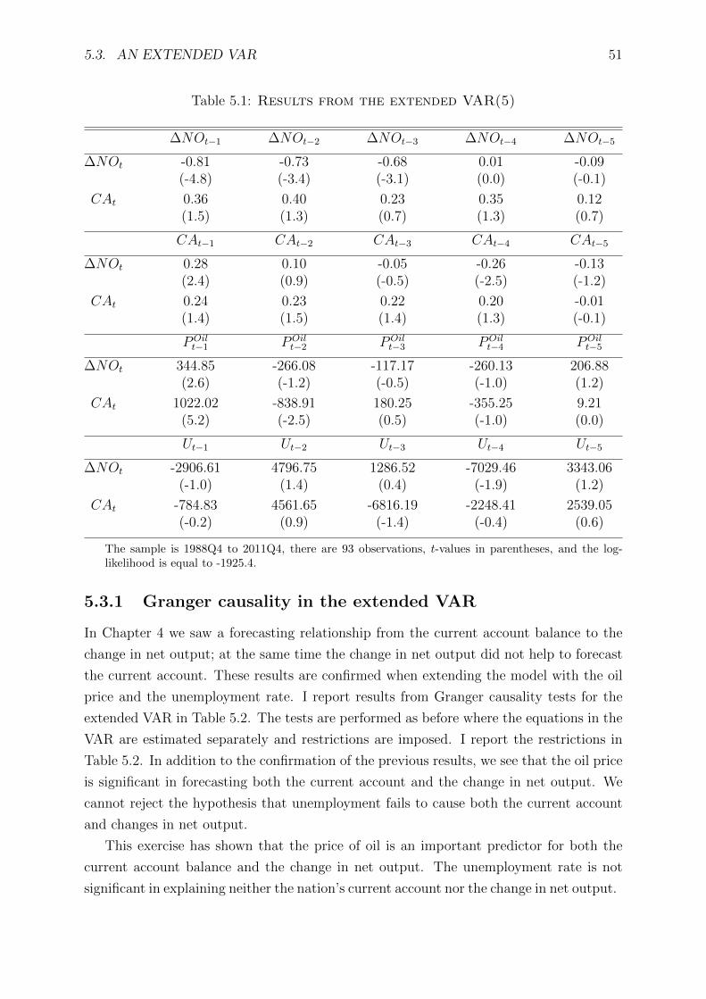
5.3. AN EXTENDED VAR 51
Table 5.1: Results from the extended VAR(5)
∆NOt−1 ∆NOt−2 ∆NOt−3 ∆NOt−4 ∆NOt−5
∆NOt -0.81 -0.73 -0.68 0.01 -0.09(-4.8) (-3.4) (-3.1) (0.0) (-0.1)
CAt 0.36 0.40 0.23 0.35 0.12(1.5) (1.3) (0.7) (1.3) (0.7)
CAt−1 CAt−2 CAt−3 CAt−4 CAt−5
∆NOt 0.28 0.10 -0.05 -0.26 -0.13(2.4) (0.9) (-0.5) (-2.5) (-1.2)
CAt 0.24 0.23 0.22 0.20 -0.01(1.4) (1.5) (1.4) (1.3) (-0.1)
POilt−1 POil
t−2 POilt−3 POil
t−4 POilt−5
∆NOt 344.85 -266.08 -117.17 -260.13 206.88(2.6) (-1.2) (-0.5) (-1.0) (1.2)
CAt 1022.02 -838.91 180.25 -355.25 9.21(5.2) (-2.5) (0.5) (-1.0) (0.0)
Ut−1 Ut−2 Ut−3 Ut−4 Ut−5
∆NOt -2906.61 4796.75 1286.52 -7029.46 3343.06(-1.0) (1.4) (0.4) (-1.9) (1.2)
CAt -784.83 4561.65 -6816.19 -2248.41 2539.05(-0.2) (0.9) (-1.4) (-0.4) (0.6)
The sample is 1988Q4 to 2011Q4, there are 93 observations, t-values in parentheses, and the log-likelihood is equal to -1925.4.
5.3.1 Granger causality in the extended VAR
In Chapter 4 we saw a forecasting relationship from the current account balance to the
change in net output; at the same time the change in net output did not help to forecast
the current account. These results are confirmed when extending the model with the oil
price and the unemployment rate. I report results from Granger causality tests for the
extended VAR in Table 5.2. The tests are performed as before where the equations in the
VAR are estimated separately and restrictions are imposed. I report the restrictions in
Table 5.2. In addition to the confirmation of the previous results, we see that the oil price
is significant in forecasting both the current account and the change in net output. We
cannot reject the hypothesis that unemployment fails to cause both the current account
and changes in net output.
This exercise has shown that the price of oil is an important predictor for both the
current account balance and the change in net output. The unemployment rate is not
significant in explaining neither the nation’s current account nor the change in net output.

52 CHAPTER 5. A DISCUSSION OF THE REJECTION
Current Account Fitted
1990 1995 2000 2005 2010
0
50000
100000Current Account Fitted
Change in Net Output Fitted
1990 1995 2000 2005 2010
−25000
0
25000
Change in Net Output Fitted
Figure 5.1: The figure plot the graphical fit for a general VAR(5) given in equation (5.1)and (5.2).
Table 5.2: Granger causality in the extended VAR(5)
The equation for the current account (equation (5.1))Hypothesis Restrictions F -value P -value
∆NO fails to cause CA β11 = · · · = β15 = 0 0.8 0.55
POil fails to cause CA δ11 = · · · = δ15 = 0 5.8 0.00
U fails to cause CA γ11 = · · · = γ15 = 0 1.2 0.33
The equation for the change in net output (equation (5.2))Hypothesis Restrictions F -value P -value
CA fails to cause ∆NO α21 = · · · = α25 = 0 2.5 0.04
POil fails to cause ∆NO δ21 = · · · = δ25 = 0 3.0 0.01
U fails to cause ∆NO γ21 = · · · = γ21 = 0 0.9 0.48
The sample period is 1988Q4 to 2011Q4 and there are 91 observations.

Chapter 6
Concluding remarks
This thesis has examined the intertemporal approach to the current account for quarterly
Norwegian data for the period 1981 to 2011. In Chapter 2 I presented a dynamic model
for a small open economy where a rational forward-looking agent gets utility from con-
sumption. The model was solved by maximizing the agent’s lifetime utility subject to a
budget constraint and a no-Ponzi game condition. A key element in this model is the
result that the one-period consumption level is a constant share of the permanent value
of lifetime income. This result is known as the permanent income hypothesis. The model
predicts full consumption smoothing. I have shown that the optimal decision path for
the consumer, under a set of assumptions, can be described as a present-value relation-
ship between future changes in net output and the nation’s current account balance. If
income is expected to decline in the future, the optimal strategy is to save today to keep
the consumption level constant, if income is expected to rise; the optimal strategy is to
borrow today.
In Chapter 4, I tested the present-value relationship implied by the intertemporal
model by using a VAR for Norwegian data. Previous studies on this subject are not very
convincing; the intertemporal approach to the current account is frequently rejected in
the literature, with some exceptions.
I presented three formal tests of the validity of the PVM. The PVM can be derived from
imposing cross-equation restrictions on a general VAR. I test these restrictions where the
null-hypothesis is that these restrictions are valid. All three tests reject the restrictions,
and therefore also the PVM, on the 1 percent significance level.
On the other hand, my analysis has shown some matching attributes between the
model and the actual data. The graphical fit of the model is good; the correlation co-
efficient between the actual and predicted current account series is equal to 0.97. Since
the current account is used to smooth consumption against future changes in net output,
the current account should be as good as any predictor of changes in net output. I find
a one-way Granger causality from the current account to changes in net output, so I can
confirm that the current account contains valuable information for explaining changes in
53

54 CHAPTER 6. CONCLUDING REMARKS
net output.
So, why is the model rejected? First, it is possible that consumption is a function
of current income and the permanent income hypothesis is false. Secondly, when testing
the model, we are actually testing several hypotheses; the main one is the consumption-
smoothing behavior of the consumer, but we are also testing a hypothesis about rational
agents, perfect capital mobility, and a quadratic utility function. When rejecting the
model we cannot say which of the hypotheses that is the source of the rejection, nor can
we know if there is more than one of them who are responsible.
References
Agenor, P-R., C. Bismut, P. Cashin, and C. J. McDermott C. J. (1999), “Consumption
smoothing and the current account: evidence for France, 1970–1996”, Journal of Inter-
national Money and Finance, 18:1-12.
Bergin, P. R. and S. M. Sheffrin (2000), “Interest rates, exchange rates and present value
models of the current account”, The Economic Journal, 110:535–558.
Bouakez, H. and T. Kano (2009), “Tests of the present-value model of the current ac-
count: A note”, Applied Economics Letters, 16:1215–1219.
Breusch, T. S. (1978), “Testing for autocorrelation in dynamic linear models”, Australian
Economic Papers, 17:334–355.
Brooks, C. (2008), Introductory Econometrics for Finance, Cambridge University Press,
Cambridge, UK.
Campbell, J. Y. and R. J. Shiller (1987), “Cointegration and tests of present value mod-
els”, Journal of Political Economy, 95:1062–1088.
Campbell, J. Y. (1987), “Does saving anticipate declining labor income? An alterna-
tive test of the permanent income hypothesis”, Econometrica, 55:1249–1273.
Dickey, D. A. and W. A. Fuller (1979), “Distribution of the estimators for autoregressive
time series with a unit root”, Journal of the American Statistical Association, 74:427–431.
Engle, R. F. (1984), “Wald, Likelihood ratio, and Lagrange Multiplier Tests in Econo-
metrics”, in: Handbook of Econometrics, Volume II, Edited by Z. Griliches and M.D.
Intriligator, Elsevier Science Publishers BV.
Friedman, M. (1957), A Theory of the Consumption Function. Princeton University
Press, Prineceton, N.J.
55

56 REFERENCES
Ghosh, A. R. (1995), “International capital mobility amongst the major industrialised
countries: Too little or too much?”, The Economic Journal, 105:107–128.
Ghosh, A. R., and J. D. Ostry (1997), “Macroeconomic uncertainty, precautionary saving,
and the current account”, Journal of Monetary Economics, 40:121–139.
Godfrey, L. G. (1978), “Testing against general autoregressive and moving average error
models when the regressors include lagged dependent variables”, Econometrica, 46:1293–
1301.
Gourinchas, P-O. and O. Jeanne (2011), “Capital flows to developing countries: The
allocation puzzle”, unpublished paper.
Graham, A. (1981), Kronecker Products and Matrix Calculus With Applications, Ellis
Horwood Limited, Chichester, England.
Granger, C. W. J. (1969), “Investigating causal relations by econometric models and
cross-spectral methods”, Econometrica, 37:424–438.
Hall, R. E. (1978), “Stochastic implications of the life cycle-permanent income hypothesis:
Theory and evidence”, Journal of Political Economy, 86:971–987.
Hamilton, J. D. (1994), Time series analysis. Princeton University Press, Prineceton,
N.J.
Hayashi, F. (2000), Econometrics. Princeton University Press, Prineceton, N.J.
Iscan, T. B. (2002), “Present value tests of the current account with durable consump-
tion”, Journal of International Money and Finance, 21:385–412.
Jarque, C. M. and A. K. Bera (1987), “A test for normality of observations and re-
gression residuals”, International Statistical Review, 55:163–172.
Kose, A., E. Presad, K. Rogoff and S. Wei (2006), “Financial Globalization, a Reap-
praisal”, IMF Working Paper 06/189.
Lucas, R. (1976), “Econometric Policy Evaluation: A Critique”, Carnegie-Rochester Con-
ference Series on Public Policy, 1:19–46.
57
Nason, J. M. and J. H. Rogers (2006), “The present-value model of the current account
has been rejected: Round up the usual suspects”, Journal of International Economics,
68:159–187.
Obstfeld, M. and K. Rogoff (1995), “The intertemporal approach to the current account”,
in: Grossman G.M and K. Rogoff (Eds.), Handbook of International Economics, 3. Else-
vier Science BV.
Obstfeld, M. and K. Rogoff (1996), Foundations of International Macroeconomics. MIT
Press. Cambridge, MA.
Otto, G. (1992), “Testing a present-value model of the current account: Evidence from
US and Canadian time series”, Journal of International Money and Finance, 11:414–430.
Razin, A. (1995), “The dynamic-optimizing approach to the current account: Theory and
evidence”, in: P.B. Kenen, ed., Understanding interdependence: The macroeconomics of
the open economy. Princeton University Press, Princeton, N.J.
Sachs, J. (1982), “The current account in the macroeconomic adjustment process”, Scan-
dinavian Journal of Economics, 84:147–159.
Sheffrin, S. M. and W. T. Woo (1990), “Present value tests of an intertemporal model of
the current account”, Journal of International Economics, 29:237–253.
White, H. (1980), “A heteroskedasticity-consistent covariance matrix estimator and a
direct test for heteroskedasticity”. Econometrica, 48:817–838.
Wu, J. (2000), “Mean reversion of the current account: evidence from the panel data
unit-root test”, Economic Letters, 66:215–222.

58 REFERENCES
Appendices
Appendix A: Derivation of the PVM
Let us start with equation (2.16)
CAt = NOt − EtNOt.
Then, use NOt = r1+r
∞∑s=t
(1
1+r
)s−tNOs and we get
CAt = NOt − Etr
1 + r
∞∑s=t
(1
1 + r
)s−tNOs.
This expression can be written as
CAt = NOt − Etr
1 + r
[(1
1 + r
)0
NOt +
(1
1 + r
)1
NOt+1 +
(1
1 + r
)2
NOt+2 + . . .
]
= Et
1
1 + rNOt − r
[(1
1 + r
)2
NOt+1 +
(1
1 + r
)3
NOt+2 +
(1
1 + r
)4
NOt+3 + . . .
]
=1
1 + rNOt −
r
(1 + r)2EtNOt+1 −
r
(1 + r)3EtNOt+2 −
r
(1 + r)4EtNOt+3 − . . .
=1
1 + rNOt −
(1
1 + r− 1
(1 + r)2
)EtNOt+1 −
(1
(1 + r)2− 1
(1 + r)3
)EtNOt+2 − . . .
=1
1 + rNOt −
1
1 + rEtNOt+1 −
(1
1 + r
)2
EtNOt+1 −(
1
1 + r
)2
EtNOt+2 − . . .
=1
1 + r(NOt − EtNOt+1) +
(1
1 + r
)2
(EtNOt+1 − EtNOt+2) + . . .
= − 1
1 + rEt∆NOt+1 −
(1
1 + r
)2
Et∆NOt+2 −(
1
1 + r
)3
Et∆NOt+3 − . . . .
And by using the summation operator we get
CAt = −∞∑
s=t+1
(1
1 + r
)s−tEt∆NOs.
A1
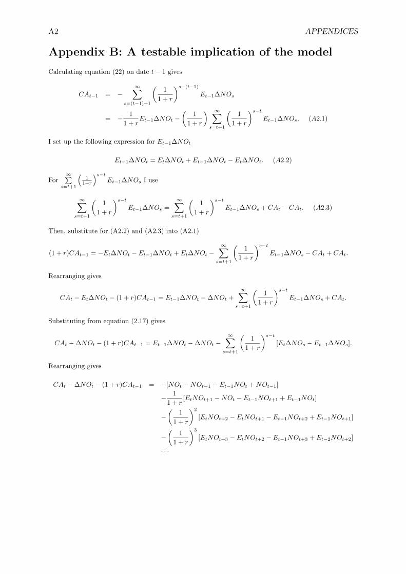
A2 APPENDICES
Appendix B: A testable implication of the model
Calculating equation (22) on date t− 1 gives
CAt−1 = −∞∑
s=(t−1)+1
(1
1 + r
)s−(t−1)Et−1∆NOs
= − 1
1 + rEt−1∆NOt −
(1
1 + r
) ∞∑s=t+1
(1
1 + r
)s−tEt−1∆NOs. (A2.1)
I set up the following expression for Et−1∆NOt
Et−1∆NOt = Et∆NOt + Et−1∆NOt − Et∆NOt. (A2.2)
For∞∑
s=t+1
(1
1+r
)s−tEt−1∆NOs I use
∞∑s=t+1
(1
1 + r
)s−tEt−1∆NOs =
∞∑s=t+1
(1
1 + r
)s−tEt−1∆NOs + CAt − CAt. (A2.3)
Then, substitute for (A2.2) and (A2.3) into (A2.1)
(1 + r)CAt−1 = −Et∆NOt − Et−1∆NOt + Et∆NOt −∞∑
s=t+1
(1
1 + r
)s−tEt−1∆NOs − CAt + CAt.
Rearranging gives
CAt − Et∆NOt − (1 + r)CAt−1 = Et−1∆NOt −∆NOt +∞∑
s=t+1
(1
1 + r
)s−tEt−1∆NOs + CAt.
Substituting from equation (2.17) gives
CAt −∆NOt − (1 + r)CAt−1 = Et−1∆NOt −∆NOt −∞∑
s=t+1
(1
1 + r
)s−t[Et∆NOs − Et−1∆NOs].
Rearranging gives
CAt −∆NOt − (1 + r)CAt−1 = −[NOt −NOt−1 − Et−1NOt +NOt−1]
− 1
1 + r[EtNOt+1 −NOt − Et−1NOt+1 + Et−1NOt]
−(
1
1 + r
)2
[EtNOt+2 − EtNOt+1 − Et−1NOt+2 + Et−1NOt+1]
−(
1
1 + r
)3
[EtNOt+3 − EtNOt+2 − Et−1NOt+3 + Et−2NOt+2]
. . .

APPENDIX C: RESTRICTIONS ON THE PARAMETER MATRIX A3
CAt −∆NOt − (1 + r)CAt−1 = −(NOt −
NOt1 + r
)−(Et−1NOt −
Et−1NOt1 + r
)+
(EtNOt+1
1 + r− EtNOt+1
(1 + r)2
)−(Et−1NOt+1
1 + r− Et−1NOt+1
(1 + r)2
)+
(EtNOt+2
(1 + r)2− EtNOt+2
(1 + r)3
)−(Et−1NOt+2
(1 + r)2− Et−1NOt+2
(1 + r)3
)+ . . .
CAt −∆NOt − (1 + r)CAt−1 = − r
1 + r(NOt − Et−1NOt)
+r
(1 + r)2(EtNOt+1 − Et−1NOt+1)
+r
(1 + r)3(EtNOt+2 − Et−1NOt+2)
+r
(1 + r)4(EtNOt+3 − Et−1NOt+3)
+ . . . .
And by using the summation operator we get
CAt −∆NOt − (1 + r)CAt−1 = −r(
1
1 + r
) ∞∑s=t
(1
1 + r
)s−t(EtNOs − Et−1NOs).
Appendix C: Restrictions on the parameter matrix
The restriction is given by
eCA = −e∆NO(τΓ)(I− τΓ)−1.
The companion matrix from the VAR(4) is given by
Γ =
α11 β11 α12 β12 α13 β13 α14 β14
α21 β21 α22 β22 α23 β23 α24 β24
1 0 0 0 0 0 0 0
0 1 0 0 0 0 0 0
0 0 1 0 0 0 0 0
0 0 0 1 0 0 0 0
0 0 0 0 1 0 0 0
0 0 0 0 0 1 0 0
.
If I − τΓ is an invertible matrix, we can calculate the linear restrictions as linear relations between the
coefficients from the VAR. We can write eCA(I− τΓ) = −e∆NO(τΓ) which imply the linear restriction
eCA = τ(eCA − e∆NO)Γ. The parameter by parameter restrictions can be calculated if we note that
eCA = [0 1 0 0 0 0 0 0], e∆NO = [1 0 0 0 0 0 0 0],

A4 APPENDICES
(I− τΓ) =
1− τα11 −τβ11 −τα12 −τβ12 −τα13 −τβ13 −τα14 −τβ14−τα21 1− τβ21 −τα22 −τβ22 −τα23 −τβ23 −τα24 −τβ24−τ 0 1 0 0 0 0 0
0 −τ 0 1 0 0 0 0
0 0 −τ 0 1 0 0 0
0 0 0 −τ 0 1 0 0
0 0 0 0 −τ 0 1 0
0 0 0 0 0 −τ 0 1
,
−e∆NO(τΓ) = [−τα11 − τβ11 − τα12 − τβ12 − τα13 − τβ13 − τα14 − τβ14],
and
eCA(I− τΓ) = [−τα21 1− τβ21 − τα22 − τβ22 − τα23 − τβ23 − τα24 − τβ24].
The restrictions are then given by
α11 = α21, α12 = α22, β12 = β22, α13 = α23, β13 = β23,
α14 = α24, β14 = β24 and τβ21 = 1 + τβ11.
Appendix D: The stationarity of the VAR(4)
To evaluate the stationarity of the VAR(4), the following equation must be solved1
det(I2 −A1x−A2x2 −A3x
3 −A4x4) = 0,
which can be written as a polynomial of degree 8, the polynomial is known as the characteristic equation
of the VAR and can be written as
−0.129x8 + 0.007x7 − 0.008x6 + 0.122x5 + 0.945x4 + 0.0232x3 + 0.044x2 − 0.175x = 1.
This equation has the following solutions
x1 = 1.678, x2 = 1.049,
x3 = −1.055, x4 = −1.447,
x5 = −0.069 + 1.568i, x6 = −0.069− 1.568i,
x7 = −0.017 + 1.081i, x8 = −0.017− 1.081i,
where i is the square root of −1. All the roots of the characteristic equation lie outside the unit circle,
and the VAR(4) is stationary.
1See Hamilton (1994), Chapter 10.

APPENDIX E: SYMBOL GLOSSARY A5
Appendix E: Symbol glossary
I have tried to let one letter serve one purpose only, but in some cases a letter may have a different in-
terpretation in different parts of my thesis, when this is the case I explain the different usages. Matrices
are in uppercase bold letters while vectors are in lowercase bold letters.
Uppercase English Alphabet
A : Parameter matrix from the VAR.
B : Holdings of foreign assets.
BG: Breusch-Godfrey test statistic.
C : Private consumption.
CA: Current account balance.
E : Expectations operator.
G : Government consumption.
H : A hypothesis.
I : Investment.
I : Identity matrix.
JB: Jarque-Bera test statistic.
K : Number of regressors.
Ku: The kurtosis of a distribution.
LL: Log-likelihood value of a model.
LR: Log-likelihood ratio test statistic.
NO: Net output.
P : The price of oil.
R : Generic variable.
S : Expression for information criterion.
Sk: The skewness of a distribution.
T : Number of observations.
U : Lifetime utility in chapter 2 and unemployment rate in chapter 5.
V : Matrix of squared residuals from the VAR.
W : National wealth.
X : Generic variable.
Lowercase English Alphabet
a: Generic parameter/constant.
b: Generic parameter/constant.
c: Generic parameter/constant.
e: Vector of zeros and one unity element.
g: Penalty function in expression for information criterion.
i: Generic index.
j: Generic index.
p: Number of parameters in the VAR.
q: Limit of a generic summation.
r: Real interest rate.
s: Summation index.
t: Time index.
u: One-period utility function in chapter 2 and residuals from a regression model in chapter 3.
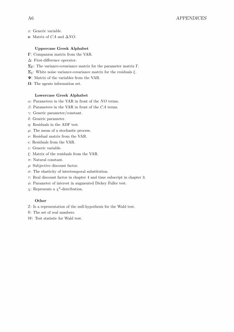
A6 APPENDICES
x: Generic variable.
z: Matrix of CA and ∆NO.
Uppercase Greek Alphabet
Γ: Companion matrix from the VAR.
∆: First-difference operator.
ΣΓ: The variance-covariance matrix for the parameter matrix Γ.
Σξ: White noise variance-covariance matrix for the residuals ξ.
Ψ: Matrix of the variables from the VAR.
Ω: The agents information set.
Lowercase Greek Alphabet
α: Parameters in the VAR in front of the NO terms.
β: Parameters in the VAR in front of the CA terms.
γ: Generic parameter/constant.
δ: Generic parameter.
η: Residuals in the ADF test.
µ: The mean of a stochastic process.
ν: Residual matrix from the VAR.
ε: Residuals from the VAR.
ε: Generic variable.
ξ: Matrix of the residuals from the VAR.
π: Natural constant.
ρ: Subjective discount factor.
σ: The elasticity of intertemporal substitution.
τ : Real discount factor in chapter 4 and time subscript in chapter 3.
φ: Parameter of interest in augmented Dickey Fuller test.
χ: Represents a χ2-distribution.
Other
I: Is a representation of the null-hypothesis for the Wald test.
R: The set of real numbers.
W: Test statistic for Wald test.