UvA-DARE is a service provided by the library of the University of Amsterdam (http://dare.uva.nl)

UvA-DARE (Digital Academic Repository)

The political economy of (de)regulation: Theory and evidence from the U.S. electricitymarketGuerriero, C.

Link to publication

Citation for published version (APA):Guerriero, C. (2010). The political economy of (de)regulation: Theory and evidence from the U.S. electricitymarket. (ACLE working paper; No. 2010-06). Amsterdam: Amsterdam Center for Law & Economics.

General rightsIt is not permitted to download or to forward/distribute the text or part of it without the consent of the author(s) and/or copyright holder(s),other than for strictly personal, individual use, unless the work is under an open content license (like Creative Commons).

Disclaimer/Complaints regulationsIf you believe that digital publication of certain material infringes any of your rights or (privacy) interests, please let the Library know, statingyour reasons. In case of a legitimate complaint, the Library will make the material inaccessible and/or remove it from the website. Please Askthe Library: http://uba.uva.nl/en/contact, or a letter to: Library of the University of Amsterdam, Secretariat, Singel 425, 1012 WP Amsterdam,The Netherlands. You will be contacted as soon as possible.

Download date: 07 Jan 2019

Electronic copy available at: http://ssrn.com/abstract=1668482

The Political Economy of (De)Regulation: Theory and Evidence

from the U.S. Electricity Market

Carmine Guerriero

Amsterdam Center for Law & Economics Working Paper No. 2010-06

The complete Amsterdam Center for Law & Economics Working Paper Series is online at: http://ssrn.acle.nl For information on the ACLE go to: http://www.acle.nl

Electronic copy available at: http://ssrn.com/abstract=1668482

The Political Economy of(De)Regulation:

Theory and Evidence from the U.S.Electricity Market.∗

Carmine Guerriero

Department of Economics and ACLE, University of Amsterdam

February 13, 2011

Abstract

The choice of whether to regulate a market or let firms compete is a key issue ineconomics. Whenever the demand is sufficiently inelastic, competition produces lowerallocative distortions but also lower expected profits and, thus, weaker incentives to in-vest in cost-reduction than regulation does. Hence, the likelihood that a society choosescompetition is higher: (i) the less salient cost-reduction is; (ii) the more limited theextent of asymmetric information and, thus, the expected profits under regulation are;(iii) the stronger the political power of the consumers is. This prediction is consistentwith U.S. electricity market data. During the 1990s, deregulation was enacted wheregeneration costs were historically lower and politicians were more pro-consumer. Also,GMM estimates show that restructuring made significantly more likely that the firmswith the lowest costs served the market to the detriment of cost-reducing investments.This evidence sheds new light on the slowdown of the deregulation wave.Keywords: Regulation; Competition; Electricity; Accountability.JEL classification: L11; L51; L94; P16.

∗I would like to thank Serra Boranbay, Anna Creti, Mikhail Drugov, Kira Fabrizio, Giulio Federico,Sander Onderstal, Clara Poletti, Carlo Scarpa, Sandro Shelegia, and seminar participants at FEEM, CSEF,UVA and at the 2010 ESNIE meeting in Cargese for useful comments. The first draft of this paper wascompleted while I was visiting the IEFE at Bocconi University. To the last extent, I gratefully acknowledgethe Institution’s support. Address: Roetersstraat 11, 1018 WB Amsterdam, The Netherlands. Phone: +31(0)205254162. Fax: +31 (0)205255318. E-mail: c.guerriero@uva.nl

“Competition is not only the basis of protection to the consumer but is the incentive to progress.

However, [. . . ] destructive competition [. . . ] may impoverish the producer and the wage earner”

(Herbert Hoover, States of the Union Address, December 2, 1930).

1 Introduction

Economists have long maintained that, even if competition assures allocative efficiency,

regulation could be better suited to stimulate the firm’s cost-reducing investment. Hence, a

benevolent government should choose between competition and regulation optimally trading

off allocative efficiency and investment inducement. Yet, market institutions are designed

by more or less pro-shareholders politicians and the extent of asymmetric information is

a function of the activity of regulators accountable to special interest groups and not to

the society at large. How, therefore, do politicians’ and regulators’ incentives shape the

allocative efficiency-investment inducement trade off when market institutions are designed?

This paper lays out a theoretical framework for thinking about this issue, and explores its

empirical implications using U.S. electricity data. In the model, I build on a wide literature

on incentives and competition (see Armstrong and Sappington, [2006]), and I compare two

market institutions in a world in which the demand is inelastic and the firms can commit

a cost-reducing investment before privately learning their cost. Under competition, produc-

tion is assured by two firms. Each firm serves all the market at the price proposed by the

opponent when able to undercut it. When the bids are the same, the two firms split the mar-

ket. Under regulation, instead, production is assured by a local monopoly. In equilibrium,

competition produces lower allocative distortions but also lower expected profits and, thus,

2

weaker incentives to invest in cost-reduction than regulation does. Hence, the likelihood that

a society chooses competition is higher the less salient cost-reduction is and the more limited

the expected profits are because regulators have stronger political incentives to reveal the

firm’s private information. When, instead, investments affect asymmetrically the firm’s costs

and profits, a tension between consumers and shareholders arises and competition is more

often adopted the more powerful consumers are. Finally, because competition serves better

static efficiency—i.e., minimizing allocative distortions—and worse dynamic efficiency—i.e.,

stimulating investments, the relation between the average cost and market institutions is

undecided. The model’s message remains similar when competition is a’ la Cournot.

In order to test these predictions, I look at the restructuring of the U.S. electricity market.

I analyze a panel of 503 plants owned by investor owned utilities—IOUs hereafter—operating

in 43 states over the period 1981 to 1999. Public Utility Commissions—PUCs hereafter—

have classically set prices in order to assure a specific return on investment after recouping

all operating costs recognized as reimbursable during rate reviews. After having experi-

mented incentive regulation in the 1980s, many U.S. states enhanced more radical reforms

in the mid-1990s. As a result, today, several IOUs own only a small fraction of the total

generation capacity and retail rates often follow the prices clearing auction-based wholesale

markets (Fabrizio, Rose and Wolfram, 2007). Consistent with the model, deregulation was

enhanced in states where generation costs were historically lower and politicians were more

pro-consumer. Also, GMM estimates suggest that deregulation had a significant and strong

negative medium term effect on labor and fuel inputs and an insignificant effect on the plants’

efficiency to transform fuel inputs into power. This evidence, along with the fact that the

new capacity entered service in the last two decades was built mainly by IOUs operating in

3

non restructured markets (Joskow, 2008), confirms the model’s intuition according to which

competition assures that the firm with the most efficient technology serves the market for

a given cost distribution but that the latter will be more favorable under regulation. These

results shed new light on the recent slowdown of the deregulation wave (EIA, 2003).1

Even if several studies (Aghion et al., 2005; Alesina et al, 2005; Bushnell and Wolfram,

2005; Zhang, 2007; Fabrizio, Rose and Wolfram, 2007; Parker, Kirkpatrick and Zhang, 2008)

have reported evidence suggesting that deregulation can deliver lower input uses and costs,

no previous paper has developed a formal theoretical and empirical framework to shed light

on its introduction.2 In this perspective, the key contribution of the present paper is to prove,

for the first time, that the choice of market institutions is essentially based on an allocative

efficiency-investment inducement trade off and to explore the related political economics.3

The rest of the paper is organized as follows. Section 2 describes the institutions of the

U.S. electricity market as an example of the general setting studied in the model. Section 3

illustrates the basic static versus dynamic efficiency trade off solved by society when designing

market institutions. Section 4 evaluates the role of regulators’ and politicians’ incentives.

Section 5 states the predictions which are tested in section 6; section 7 concludes. The

appendix gathers the proofs, the tables and a detailed description of the data.

1The present paper also explains the start of 20th century switch from a municipal regulation with its typicalhold-up problems to a state regulation assuring a fair rate of return on investment: these reforms wereenhanced where capacity shortages were more severe and residential penetration rates lower (Knittel, 2006).

2Recent papers (Teske, 2004; Duso and Roller, 2003; Knittel, 2006; Zhang, 2007; Belloc and Nicita, 2010;Craig and Savage, 2010; Guerriero, 2010a; Potrafke, 2010) provide empirical evidence of the relevance forregulatory reforms of the mechanisms identified in my model. Also, Benmelech and Moskowitz (2010) showsthat the extent of financial regulation falls with its costs and the political power of wealthy incumbents whoare interested in limiting political entry by applying restrictions to lending.

3As a consequence, the present paper is complementary not only to the well-known literature on sub-additivecosts (Baumol and Klevorick, 1970) and to the classic contributions on market failures (Stiglitz, 1989) butalso to a wide body of research seeing the rise of the regulatory state as a response to the risk that themajority of market participants is coerced by a subgroup of more powerful special interests (Stigler, 1971;Glaeser and Shleifer, 2003) or of similarly powerful untrustworthy agents (Aghion et al., 2010; Pinotti, 2010).

4

2 Institutions

Reforming the U.S. power market: firms’, regulators’ and politicians’ incentives.—As

anticipated above, restructuring initiatives have fundamentally changed the way plant owners

earn revenues. At the wholesale level, plants sell through either newly created spot markets

or long-term contracts based on expected spot prices. In the spot market, plant owners bid a

supply schedule for power. The dispatch order is set by the bids, and the bid of the marginal

plant is paid to all plants that are dispatched. Hence, high-cost plants are forced down in

the dispatch order, reducing expected revenues. The details of the restructuring initiatives

and, in particular, whether to disintegrate the firm, whether to participate in a pool of

wholesale markets, and the duration of each deregulation phase are decided during rate

reviews (Shumilkina, 2009). The latter are structured in quasi-judicial hearings presided

by the PUC commissioners, open to all the interested parties—i.e., the firms, consumer

advocates, and the media, and usually triggered either by IOUs in response to cost shocks or

periodically by the PUC. In the case of restructuring, almost all reviews have been required by

one or both state houses with the intention of obtaining a final decision assuring “adequate,

safe, reliable, and efficient energy services at fair and reasonable prices” (EIA, 2003, page

24). Accordingly, the focus of the regulatory orders preceding any legislative decision has

been on the impact of restructuring on both expected prices and expected investment levels.4

During the hearings the commissioners examine experts and collect the evidence: given

the extensive media coverage, this information-gathering role is the key task considered for

the selection and retention of these officials (Gormley, 1983; Friedman, 1991).5

4Coherently with the message of the model discussed below, the expectation of heavy dynamic inefficiencieswas considered the main obstacle to the deregulation processes in Louisiana and Mississippi (EIA, 2003).

5This role is coherent to the US Administrative Procedure Act (APA) prescriptions: “the proponent of a

5

From institutions to theory.—On top of the above discussion, I will assume that the choice

between competition and regulation is taken by a planner who maximizes a weighted average

of the net consumer surplus and the firm’s utility, and that the weight attached to the latter

increases with the saliency of cost-reduction. Also, when investment are not in the interest

of consumers, such weight is higher the stronger is the political power of shareholders. This

setting captures the objective of the rate reviews and the fact that, even if during the hearings

the widest consensus among parties is needed, politicians can bias the institutional choice

in order to favor their constituency. Finally, in accordance with the institutional role of

commissioners, I maintain that the regulatory contract can be contingent on a signal whose

observable precision increases with the effort exerted by a regulator. Should the latter be

the case, the regulator will be rewarded on the basis of such precision.

3 The Static Versus Dynamic Efficiency Trade Off

The model builds on Laffont and Tirole (1993), and Armstrong and Sappington (2006).

First, I will compare competition and regulation in a world in which the firm can sink cost-

reducing investments before observing its production efficiency and the regulator acts as

perfect agent of society. This exercise stresses the relation between dynamic inconsistency

in investment and the design of regulatory institutions. Next, I will evaluate the role played

by the regulator’s career concerns and by the preferences of the politicians constituency.

Preliminaries.—The representative demand for the homogeneous good is q (p) > 0 for p ∈

[0, p) and 0 for p ≥ p with q′ (p) < 0 for p ∈ [0, p]. Both q (p) and p are common knowledge.

rule or order has the burden of proof [...] a rule or order [needs to be] supported by and in accordance withreliable, probative, and substantial evidence” (Title 5, Pt. 1, Chapter 5.II, 556(d)).

6

Production is assured by either one regulated firm or two competitive ones. The marginal

and average cost ci equals either cL or cH < p with the same probability and ∆ ≡ cH−cL > 0.

While the cost distribution is common knowledge, the realization of ci is private information

of the firm.6 Should the correlation between types be positive or the probability of having

low cost be generic, none of the model’s results will be affected (see footnote 10 and 12).

Firms maximize the rent, Ui, which is the sum of the profits π (p, ci) ≡ q (p) (p− ci) and

a transfer t ≥ 0 which can be positive only under regulation. The social welfare is given by

the consumer gross surplus S (p) =∫ p

pq (x) dx plus α ∈ [0, 1) times the firm’s rent minus

the transfer evaluated at the shadow cost of public funds 1 + λ > 1: S (p) + αU − (1 + λ) t.

Two are the key features of this welfare function. First, the assumption that society values

consumer welfare at least as much as that of shareholders can be justified by the fact that

consumers are less wealthy and can be relaxed provided that α < 1 + λ (see Armstrong and

Sappington, [2007]). Second, a transfer t reduces the social welfare by (1 + λ) t because it is

financed through distortionary taxes. Should the regulated firm be private as in the market

studied below, then only the model’s interpretation will change: i.e., t will represent the firm

manager’s reward and λ the shadow cost of the managerial moral hazard constraint (see

Joskow and Schmalensee, [1986]). I also assume that the expected social welfare function is

strictly concave and I focus on the empirically relevant case of inelastic demand:

A1: The demand satisfies q′′ (p) (p− cL) + q′ (p) < 0 and εp,q = −q′ (p) p/q (p) < 1.

The timing.—The design of institutions and production proceeds according to this time line:

t = 1.—The planner chooses between regulation and competition on the basis of the

6Two key avenues for future research are: 1. to include in the model the indirect effects of market pressuresworking through the reduction of agency costs within the firms (Baggs and de Bettignies, 2007); 2. to haveci linearly decreasing with a contractible cost reducing effort as in Laffont and Tirole (1993). In the last case,the model’s results will depend on the properties of both the disutility of effort and the demand function.

7

sum of the expected welfare and a mean zero shock δ to her preferences for regulation; δ is

distributed according to the density f on the support [−∞,∞]. If regulation is chosen, a

regulator, who acts as a perfect agent of the planner, offers the monopoly a menu of (ti, pi)

pairs conditional on the firm’s report of its type but not on eventual investments.

t = 2.—Each firm eventually commits an unobservable investment I which, at the cost

ψ (I), increases the probability of cL to (1 + I)/2. The firms’ investment choices are con-

temporaneous under competition. The function ψ (·) is increasing, strictly convex and such

that ψ (0) = 0, ψ (I) > 0 for all I > 0 and limI→1 2ψ′ (I) ≥ S (cL) − S (cH).7

t = 3.—Each firm discovers its piece of private information, which is the realization of ci.

t = 4.—Under regulation the planner asks the firm to report ci and the corresponding

contract is executed. Under competition each firm bids a price and the firm with the lowest

bid serves the whole market at the price played by the opponent. If the two bids are equal, the

market is evenly split. Clearly, the equilibrium is the same as under symmetric information.8

In interpreting the generality of the foregoing, several observations should be borne in

mind. First, the shock δ captures the existence of long-lived determinants of regulation, like

the level of trust in the society (Aghion et al., 2010; Pinotti, 2010), unrelated to technolog-

ical and political forces. Second, because the firm’s cost-reducing investments are financed

through the expected rent, α is a measure of society’s dynamic efficiency concerns. Third,

the assumption according to which the regulator is benevolent can be relaxed as clarified in

section 4.2. Finally, I focus on Bertrand competition because this conduct bears the closest

7Such investment technology has been extensively studied within both regulated (Laffont and Tirole, 1993)and competitive (Raith, 2003; Baggs and de Bettignies, 2007; Vives 2008) environments.

8The interaction is strategically similar to a second price auction and both types prefer truth-telling. Indeed,while the cH type is indifferent, the cL type strictly prefers to report the truth when faced with a cH opponentand weakly prefers to play cL, in order to exhaust any incentive to undercut, if faced with a cL counterpart.

8

resemblance to the functioning of the second-price auction based wholesale markets used

to price power in the restructured U.S. electricity markets and illustrated above. Building,

however, on data from the same market, Bushnell, Mansur, and Saravia (2008) stress the

relevance of considering capacity constraints and long-term contracts to correctly assess the

impact of restructuring on market outcomes. To the last extent, section 4.3 will explain why

the model’s main message is preserved when it is assumed, instead, that the competition is

a’ la Cournot and/or the regulator can commit to reimburse investment expenses.

Regulating a monopoly with unknown costs.—Under regulation, the planner grants a reserva-

tion wage of 0 to the regulator and a legal monopoly to one firm. The regulator exploits the

revelation principle (Myerson, 1979) and announces that she will set price pi and deliver a

transfer ti whenever the report is ci. Because the planner dislikes leaving a positive rent to the

firm and prefers to let both firms produce,9 the equilibrium envisions a binding low cost firm’s

incentive compatibility constraint—i.e., q (pL) (pL − cL) + tL = q (pH) (pH − cL) + tH—and

a binding high cost firm’s individual rationality constraint—i.e., UH = 0. The first con-

straint assures that a low cost firm truthfully reports its type, the second that a high cost

firm operates. Thus, the low cost firm enjoys a rent UL = ∆q (pH) > 0. Let wi (pi, ci) =

S (pi) + (1 + λ)πi (pi, ci). For a given equilibrium investment IR, the planner maximizes

WR = (1/2)(

1 + IR)

[wL (pL, cL) − (1 + λ− α) ∆q (pH)] + (1/2)(

1 − IR)

wH (pH , cH).

Differentiating this expression with respect to pL ≥ 0 and pH ≥ 0 reveals that the high cost

firm’s allocation is distorted in such a way that the regulator is able to achieve the exact

level of expected welfare were the firm’s costs observable but the high marginal cost equal

9This is always the case whenever the planner, if indifferent between giving up production by the cH type andoffering a contract to both types, prefers the second option. Indeed, the planner will never strictly preferthe first option for every probability (1 + v)/2 of c = cL and every p because (1 − v)S (cH (v)) ≥ 0.

9

to cH ≡ cH +(

1 + IR)(

1 − IR)−1

[

1 − α (1 + λ)−1] ∆ > cH . While the regulator increases

pH over cH and reduces tH in order to limit the informational rent, she does not distort the

firm’s activities when the report is cL because there is no incentive to understate the cost.

The equilibrium is achieved through the Ramsey price obtained maximizing wL (·) for cost

cL and wH (·) for cost cH . Thus, the regulator fixes pL = cL and pH = cH (the monopolist

price) when λ is zero (large) because transfers entail no social costs (large distortions).

Competition.—Following Vives (2008), I focus on symmetric investment profiles. Given an

equilibrium investment level IC , the price will equal cH except when both firms have low

cost. Also, the firm’s rent will be positive only when it has the low marginal cost while its

rival has the high one, which happens with probability (1/4)

[

1 −(

IC)2

]

. In this case, the

firm’s rent will be ∆q (cH). As a result, the expected social welfare under competition is:

WC =(1+IC)

2

4S (cL) +

(1−IC)2+2−2(IC)

2

4S (cH) +

1−(IC)2

2α∆q (cH) .

3.1 Comparison

I maintain in the following that λ equals 0: this last assumption is relaxed in section 4.3.

The firm chooses Ij with j ∈ {R,C} to maximize expected rents minus investment costs.

Under regulation, this means solving the strictly concave program

IR = arg maxI≥0

(1/2) (1 + I) ∆q(

cH

(

IR))

− ψ (I) (1)

with cH ≡ cH+(

1 + IR) (

1 − IR)−1

(1 − α) ∆. Under competition, instead, the firm solves:

IC = arg maxI≥0

(1/4) (1 + I)(

1 − IC)

∆q (cH) − ψ (I) . (2)

10

The appendix shows that: 1. both IR and IC are positive and strictly lower than the socially

optimal investment level I∗ < 1; 2. the extent of underinvestment is wider under competition.

In this last case, the firm obtains a positive rent on a larger demand but less often: in

particular, half of the time when IC = IR = 0. Yet, whenever the demand is inelastic,

the higher probability of rents, which is a price effect, more than compensates the fall in

demand, which is a quantity one, and IR > IC . Also, underinvestment is worsened under

Bertrand competition due to the mix of the positive correlation between types introduced

by the investment technology, and the strategic complementarity between firms’ pricing

decisions.10 In t = 1 competition is chosen when WC > WR + δ that, for δ = 0, rewrites as:

2(

1 − IR)

[S (cH) − S (cH)] + 2

[

1 −(

IC)2

]

α∆q (cH) >

[

1 + 2(

IR − IC)

−(

IC)2

]

[S (cL) − S (cH)] .

(3)

For IC = IR = 0 the comparison in (3) can be restated as

12

[

S(cL)+S(cH)2

− S(cL)+S(cH)2

]

> 12

{

S(cL)+S(cH)2

− [S (cH) + α∆q (cH)]}

.

As this last inequality shows, when investment are unavailable, competition always outper-

forms regulation if the firms have the same type (see the left hand side); when however the

types are different, regulation could deliver a lower mean price when the demand is suffi-

ciently elastic and α is small (see the right hand side). Also for IC = IR = 0, a rise in α

undoubtedly enhances the likelihood that competition is adopted because it increases more

the expected rent under competition than it curbs the distortions under regulation.11

10The incentives to invest are maximized when there is no ex post correlation between types and minimizedwhen such correlation is the highest at IC = 1. Should the ex ante correlation between types be ρ > 0, themodel’s results will survive because the rent will be falling with ρ and thus still lower under competition.

11This is because ∆ (q (cH) − q (cH)) > 0. Notice that, in this case, provided that 2 [S (cH) − S (cH)] >S (cL) − S (cH), competition will outperform regulation for every value of α.

11

This comparison changes dramatically when firms can invest in cost reduction. As in-

equality (3) suggests, a rise in α not only fosters investment under regulation but entails also

a double countervailing impact on allocative distortions. The latter are relaxed due to the

higher social value of investment inducement but also strengthen because of the more favor-

able distribution of types. As the appendix shows: 1. the social value of the last indirect

effect is smaller than the one brought by the change in IR; 2. provided that the investment

technology is sufficiently effective, the social value of the fall in allocative distortions due

to the higher investment concerns is higher than the extra value carried by the firm’s rent

under competition. As a result, the probability of adopting regulation rises with α under

the following mild condition, which can be relaxed at the cost of more cumbersome algebra:

A2: ψ′ (1/2) ≤ (∆/8) q (cH).

Proposition 1: Under assumptions A1 and A2, the probability of competition is chosen

falls with the society’s investment concerns α.12

This belongs to a series of findings showing that institutions curbing rent-extraction could

be optimal if expropriation of sunk investments is an issue. While, for instance, Sappington

(1986) focuses on institutions preventing the planner from observing the firm’s true costs,

Guerriero (2010b) shows that appointment rules limiting the regulator’s incentive to provide

information on the firm’s true cost are found where investment shortages are more dramatic.

Crucially, the model shows that the possibility of committing cost-reducing investments

makes regulation more useful and transforms market design into a trade-off between static

and dynamic efficiency. The more concerned society is with cost reducing investments—

12Clearly, the patterns summarized in proposition 1 as well those discussed in the remaining part of thetheoretical section hold true when the probability of c = cL is equal to the generic value (1 + v)/2; in this

case, cH will equal cH +(

1 + IR) (

1 − IR)

−1

(1 + v) (1 − v)−1

(1 − α) ∆.

12

because, for instance, past costs have been persistently high or higher than those in bordering

regions—the lower is the probability of adopting competition. Yet, this statement needs to

be qualified. Indeed, on one hand, regulation becomes less and less appealing the thinner is

the asymmetry in information and so the stimulus to invest. On the other hand, a tension

between shareholders and consumers arise when investment returns accrue more to the ex

post rent than to the net consumer surplus. In the following, I will discuss these two points.

4 Information and Politics

Next, I will explore the political economics of the allocative efficiency-investment induce-

ment trade off and assess how robust the model’s message is to alternative assumptions.

4.1 Capture and Regulators’ Implicit Incentives

As seen above, top-level regulators respond to implicit incentives and not to performance-

based contracts and, in the case of the market studied in the empirical section below, they are

simply either elected or appointed on the base of their information-gathering effort. Building

on these observations, I consider the following information gathering technology.

In t = 1 the planner directly offers the firm a menu of (ti, pi) pairs conditional on the

firm’s report and the realization of a signal on ci that she observes between t = 3 and

t = 4. The signal is such that, if c = cL, with probability γ ∈ [0, 1] the planner sees cL and

implements the full information contract and with probability 1−γ she remains uninformed.

If c = cH , she remains uninformed throughout.13 Whenever uninformed she asks the firm

13Even if under different information structures the precision of the signal can increase allocative distortions(Boyer and Laffont, 2003), only the actual structure captures the fact that, in the U.S. electricity market,rate reviews are aimed at proving that the firm is of the cL type. Accordingly, Fremeth and Holburn (2010)

13

to report its type. The observable precision has technology γs = θes where θ ∈ [0, 1] is the

regulator’s random ability, es ∈ [0, 1] the information gathering effort, and s = {E,A} the

type of implicit incentives to which the regulator is subject to. The ability θ has mean θ and

is drawn from a truncated normal density g with g(

θ)

> 1.14

Information gathering happens between t = 3 and t = 4; during this lapse of time, first

Nature chooses θ, then the signal is observed by the planner, finally the precision γs is revealed

and the regulator rewarded on its base. The regulator maximizes B + τ [T (es) − C (es)],

where τ measures the value of the net implicit rewards relative to the bribes B offered by

the firm and the effort cost function is such that C (0) = 0, C ′ > 0, C ′ (0) < ∞, C ′′ > 0,

limes→1C′ (es) = ∞. For what concerns implicit rewards, as suggested by Alesina and

Tabellini (2007), while elected officials are held accountable by voters, appointed ones are

career concerned. In particular, elected regulators want to maximize the probability that

the realized precision is higher than the one obtained by an incumbent with mean ability

θ so that TE (eE) = Pr{

eE ≥ θeexp}

where eexp is the voters’ expectation over effort. Ap-

pointed regulators, instead, want to maximize society’s perception of their ability given the

precision’s realization or TA (eA) = Eθ [Eθ (θ |γA, eAexp )] where Eθ [·] denotes the regulator’s

unconditional expectation over γA and Eθ society’s expectation over θ conditional on γA.

For a given equilibrium effort es, the evaluators estimate θ as ξs/es. Hence, a rise in

effort delivers marginal benefits θ/

eA under appointment and g(

θ) (

θ/

eE)

under election.15

Differently from the case of appointment, under election the effect of a rise in effort on

find that better informed PUCs implement less often rate increases and more often rate decreases.14This is a mild requirement in the market studied below being the regulators’ biographies very similar (Gorm-

ley, 1983). Guerriero (2010a, b) shows that the model’s message will be unaffected should: 1. the realizationof γs be unobservable; 2. the precision technology be linear; 3. the regulator care also about social welfare.

15While the marginal benefit of effort always falls with es, the marginal cost of effort is increasing: this impliesthat the solution to the regulator’s problem is unique and interior (see Guerriero, [2010b]).

14

the estimated talent is multiplied also by the impact of a change of the estimated talent

on the probability of re-election: this last marginal effect is g(

θ)

. The higher the latter

is the more effective is effort in swaying votes and assuring a higher probability of victory.

When g(

θ)

is greater than one, election leads to a higher equilibrium effort. This pandering

incentive effect of election is complementary to the selection one proposed by Besley and

Coate (2003) but, differently from the latter, it survives when the regulator can divert effort

from information gathering to a less socially relevant task in exchange for bribes. Indeed, as

shown in Guerriero (2010b), to preserve implicit incentives she will never exert effort only in

the socially irrelevant task.16 Thus, γE > γA and the impact of a reform from appointment

to election on the planner’s institutional choice is isomorphic to the one of a rise in the

precision γ. The expected social welfare in the supervision regime—notice the apex S—is:

WR,S = 1+IR,S

2

{

γS (cL) + (1 − γ)[

S (cL) − (1 − α) ∆q(

cSH)]}

+

1−IR,S

2

{

S(

cSH)

+(

cSH − cH)

q(

cSH)}

= 1+IR,S

2S (cL) + 1−IR,S

2S

(

cSH)

,

where cSH ≡ cH + 1+IR,S

1−IR,S(1 − γ) (1 − α) ∆. The planner’s choice is described by inequality

(3) with cSH in the place of cH and the equilibrium investment under regulation is given by:

IR,S = arg maxI≥0

(1/2) (1 + I) (1 − γ) ∆q(

cSH

(

IR,S))

− ψ (I) . (4)

As shown in the appendix, under assumption A1, a more precise signal crowds out ex ante

investment incentives; as a result, on one hand, regulation becomes less efficient in insulating

the firm from ex post expropriation of sunk investments; on the other, however, a more

16Guerriero (2010b) shows also that, when the regulator directly observes the signal, she will truthfully reportsher information whenever implicit incentives are sufficiently important—i.e., τ is sufficiently high. Thiscollusion-proofness property squares with broad evidence on the limited role of capture in the U.S. electricitymarket (see the study on pricing by Leaver [2009] and that on the rise of state regulation by Knittel [2006]).

15

limited extent of allocative distortion is needed to support incentive compatibility. While

the latter is a quantity effect, the former is a price one. Again, provided that the demand is

sufficiently inelastic, the price effect will prevail and the following will hold:

Proposition 2: Whenever assumption A1 holds and εp,q < min {εp,q, 1}, the probability

that competition is chosen rises with the signal precision γ and it is higher when the regulator

is elected provided that her effort is sufficiently effective in swaying votes or g(

θ)

> 1.17

This result is similar to that proposed by Guerriero (2010a) who documents a positive relation

between the power in term of cost-reducing effort of incentive rules and the information

gathering effort level. Yet, while such pattern is simply due to the lower need of allocative

distortions, the relation documented in proposition 2 is more subtle a goes through the effects

of a more accurate information on both allocative distortions and cost-reducing investments.

4.2 Strategic Market Institutions Selection

Institutional design could be inefficient when the firm’s investment expenses favor sharehold-

ers over consumers and both groups can influence the planner’s decision. A striking example

of these expenses are those not strictly related to service provision per se—e.g., marketing,

diffusion of smart-metering technologies, reducing the fixed cost of transmission. In order to

clarify the point in the sharpest way, I assume that: 1. the return from investment accrues

only to the firm’s rents without affecting the consumer surplus;18 2. the firm is infinitely

risk averse in the range of negative ex post utilities; 3. the planner acts as an agent of

17εp,q could be either greater or lower than one depending on the degree of convexity of ψ and the size of∆. Even in the second case, requiring that εp,q < εp,q would remain a mild assumption: in fact, reviewingprevious contributions looking at the long run residential price elasticity in different U.S. and internationalmarkets, Espey and Espey (2004) report that the median of these estimates is 0.81.

18At the cost of cumbersome algebra, the idea extends to investments benefiting asymmetrically both groups.

16

the incumbent m between the pro-shareholder party Re and the pro-consumer De; 4. the

following two periods succeed the four steps studied in section 3.1:

5. The incumbent faces an election with exogenous winning probabilities xm; next, the

winner m implements a fixed aid ρm > 0 proportional to the firm’s rent and paid out

to the firm if the investment is committed. The ex post rent becomes (1 + ρm)U .

6. The firm eventually commits an investment of fixed cost I > 0. The net expected value

of the investment is πI, with π ≡ πµ + π−

(1 − µ) > 0 and π > 0 > π−. In words, the

investment is stochastic and leads to a loss π−I with probability 1 − µ > 0.

Clearly, only the low cost firm invests whenever (1 + ρm) U j + π−I ≥ 0. Let’s also suppose

that a planner agent of a type m incumbent evaluates this ex-post participation constraint

at the shadow price χm, and the investment aid ρmUj at the shadow cost of public funds

λ. In practice, χm captures the incumbent’s willingness to encourage ex post investments.

Define x ≡ ρDexDe + ρRexRe and assume the following restrictions:

A.3: ρRe > ρDe; χRe > λ > χDe.

All in all, for δ = 0 the planner will choose competition if:

(

1 − IR)

[S (cH) − S (cH)] +

[

1 −(

IC)2

]

α∆q (cH) >1+2(IR−IC)−(IC)

2

2[S (cL) − S (cH)] +

∆ [χm (1 + x) − λx]

{

(

1 + IR,S)

q (cH) −

[

1 −(

IC)2

]

q (cH)

}

. (5)

In interpreting the foregoing, several observations should be pointed out. First, the set up

formalizes the existence of huge transfers from the federal and state governments to IOUs, fi-

nanced out of distortionary taxes and aimed to solve energy externalities—e.g., air pollution,

17

roadway congestion. As discussed by Metcalf (2008), the total energy-related tax expendi-

tures for major fuel categories investments, and the production tax credits for renewable and

advanced coal-based power sources reached 3.46 billion dollars in fiscal year 2008.19 Second,

the fact that the winning party cannot reform the market institution is consistent with the

existence of a commitment period typical of regulation (see Guerriero, [2010a]). Third, the

exogeneity of xm captures the basic idea, proposed by Besley and Coate (2003), that regu-

lation is bundled at politicians election with more salient policies. Fourth, the fact that the

pro-shareholder party is more willing to subsidize investment expenses incorporates into the

model politicians’ strategic incentives to propose and implement extremist platforms in or-

der to empower their own supporters (Glaeser, Ponzetto, and Shapiro, 2005) or to buy votes

through campaign contributions (Alesina and Holden, 2008). Again, under assumptions A1,

the expected firm’s rent would be lower under competition and:

Proposition 3: Under assumptions A1, A2 and A3, the probability that competition is

selected falls with the reformer hold on power xm and is greater if she is pro-consumer.

The actual pattern originates from the mix between the asymmetry in the parties’ preferences

and the uncertainty of elections, and it is similar to the strategic dynamic proposed by

a lively political economy tradition (Persson and Svensson, 1989; Alesina and Tabellini,

1990; Hanssen, 2004). These authors claim that a lack of permanence in office can inspire

policymakers to implement reforms aimed at tying the hands of future incumbents. In

proposition 3, a higher probability of being re-elected and fixing a larger (smaller) aid,

without facing the danger of facing a new reform, pushes a pro-shareholder (pro-consumer)

19The argument still holds when the government: 1. acts as a sponsor and increases the ex post firm’s rentswithout monetary aids if χRe > 0 > χDe ; 2. can decrease investment costs directed toward cost reduction,provided that the dynamic efficiency concerns more than outweigh the higher rent extraction needs.

18

incumbent to prefer regulation in order to guarantee an even higher profit to her constituency

(curbing underinvestment). Clearly enough, this strategic dynamics can produce inefficient

reforms (see also Faure-Grimaud and Martimort, [2003]) and, for instance, a pro-consumer

party could lean for competition despite the effective danger of dynamic inefficiencies.

In the next section, I show that the qualitative message of proposition 1, 2 and 3 continues

to stand when some of the basic model’s assumptions are either relaxed or changed.

4.3 Robustness to Alternative Assumptions

A generic number of Bertrand competitors.—The welfare under regulation remains the same

and so the direct and indirect—via both IR and q(

cH

(

IR))

—impact on it of both α and

γ. Thus, in order to conclude that the model’s patterns remain unaffected, it is enough to

check that competition produces a lower expected rent, which is the case because, as it can

be easily shown, such rent strictly falls with the number of firms N for every N > 2.

Cournot competition.—Let me assume, for simplicity, that: 1. the information about c is

complete; 2. the firm’s best replies are downward sloping or P ′ + P ′′q (ci, l, N − l) < 0

with P (·) representing the strictly decreasing inverse demand and q (ci, l, N − l) the output

choice of a type ci firm when, among the N entrants, l have type cL and N − l type cH ;

3. the entry cost, borne between stage 1 and 2, is κ ≥ 0. Because the demand is inelastic,

marginal revenues fall with the quantity sold; yet, when εp,q is not too small, an equilibrium

price strictly greater than the average marginal cost exists and, for a sufficiently low entry

cost and sufficiently efficient investment technology, the firm’s incentives to invest under

competition are weaker than those under regulation: this preserves all the model’s results.

19

A positive shadow cost of public funds.—For λ > 0 the rule giving the type dependent price

as a function of the marginal cost will be of the Ramsey type and will be implicitly defined

by pi = Ψ (ci) with Ψ ≡ ϕ−1 and ϕ (λ, pi) ≡ pi + λ (1 + λ)−1q (pi) [q′ (pi)]

−1 = ci so that

∂pi/∂ci > 0. Also, it turns out that the level of investment continues to be higher under

regulation and that the effect of a change in α and γ on the level of welfare under regulation

is multiplied by ∂pi/∂ci. Yet, provided that conditions slightly stricter than those imposed

by assumptions A1 and A2 hold, it also follows that the model’s message is unaffected.

Regulatory commitment.—Provided that an ex post participation constraint is imposed, the

level of investment under regulation, when contractible, is still inefficient and higher than

the one under competition. Besides, the rule giving price as a function of marginal cost is

unaffected (see Laffont and Tirole, [1993]); as a result, proposition 1, 2 and 3 still hold.20

When investment is not contractible, instead, the allocation of the high cost firm is distorted

even more in order to account for the moral hazard in investment constraint. Yet, it can be

shown that regulation retains its dynamic advantage and, under condition similar to those

listed in assumption A1 and A2, the model’s message survives.21

5 Empirical Implications

The basic idea of the theory is that, under reasonable conditions, while competition de-

livers more limited allocative distortions, regulation assures higher expected profits and,

20Without ex post participation constraint the first best is achieved with a fixed contract.21When the planner auctions an incentive contract as in Laffont and Tirole (1993), the low cost firm interim

expected rent is (1/2)(

1 − IR)

x1 (cH , cH) ∆q (cH) where xj(

c1, c2)

for j = 1, 2 is the probability that

firm j is chosen when firm 1 has type c1 and 2 type c2. Under symmetric auctions, this rent becomes

(1/4)(

1 − IR)

∆q (cH) and regulation would lose its dynamic advantage; yet, proposition 2 would survive.

20

consequently, produces stronger incentives to invest. As a result, competitive pressures will

be more likely when regulation leaves more limited informational rents and the reformer’s

concerns with stimulating cost-reducing investments are weaker. This was embodied in

proposition 1, 2 and 3 above and leads to the first testable prediction, which read as:

Prediction 1: The likelihood of a reform toward more competitive settings will be higher

when regulators are elected, and will fall with society’s cost-reducing investment concerns and

with the reformer hold on power. Also, it will be lower when the reformer is pro-shareholder.

My second test is motivated by the observation that while regulation yields a better

distribution of firms’ types due to the stronger incentives to invest, competition induces a

higher conditional—on the types distribution—probability that the firm with the lowest cost

serves the market. Hence, the relation between market institutions and expected average

costs is undecided. Indeed, competition will assure a lower expected average cost when[

21−(IC)

2

4+

(1+IC)2

4

]

cL +(1−IC)

2

4cH < 1+IR

2cL + 1−IR

2cH ↔

1−2(IR−IC)−(IC)2

4(cL − cH) < 0,

which could fail under the mild restrictions imposed by assumptions A1, A2 and A3. On

top of this, the second prediction deals with regulatory outcomes and reads as:

Prediction 2: The average cost could be either greater or lower under competition.

Regulation will guarantee lower expected average costs when IR − IC is sufficiently big or

IR > (1/2)

[

1 + 2IC −(

IC)2

]

. As a glance to problems (1) and (2) suggests, whether or

not the last inequality is true depends on the relative sizes of the first derivatives of the

functions q (·) and ψ (·) and on the investment concern α. Yet, provided that ψ′ is not

too small, competition would yield lower expected costs when α is sufficiently small and,

thus, the investment level under regulation cannot be enough higher than the one under

competition. This is very likely to be the case for the market that I use in the empirical

21

exercise discussed below. Indeed, two historical features of the U.S. power market are: 1. a

suboptimal technological speed (see the evidence on R&D patents in Margolis and Kammen

[1999])—i.e. a not too small ψ′; 2. that “the primary concern of regulatory commissions has

been to keep nominal prices from increasing” (Joskow, 1974, page 298)—i.e. a very small α.

6 Evidence

While between 1993 and 1998 all states held hearings on possible restructuring, just

under half the jurisdictions—23 states and the District of Columbia—enacted restructuring

legislations between 1996 and 2000.22 Yet, as widely documented by Fabrizio, Rose and Wol-

fram (2007), utilities often acted before final legislations altering in advance their behaviors.

In order to capture at best the role of expectations and have a wide enough comparison

period, I take into consideration productivity of all the large fossil-fuel steam and combined

cycle gas turbine generating plants for which data were reported to the FERC between 1981

and 1999. I restrict the sample to states for which data on the quality of the information

gathering technology and political competition are available—see the appendix. As a result,

the dataset gathers 8,059 observations on 503 plant-epochs—i.e. years over which the plant

capacity did not change more than 40 MW or the 15 percent of the capacity—operating in

43 U.S. states. I consider two dependent variables: 1. Deregulation which equals one for IOU

plants in states that restructured beginning in the year of the first formal hearing and zero

otherwise (see also Fabrizio, Rose and Wolfram, [2007]);23 2. Der Ord which equals three

22Between 1982 and 2002, twenty-three U.S. states adopted some forms of broadly defined incentive regulation(see Guerriero, [2010a]). Once considered, performance based regulation does not show complementaritieswith restructuring and its presence does not change the gist of the results discussed below.

23Should I use, instead of Deregulation, either the dummy Law, which equals one for IOU plants in states thatrestructured beginning in the year that legislation was enacted, or the dummy Retail, which equals one for

22

for states that restructured beginning in the year that legislation was enacted, two for states

that restructured beginning in the year of the first formal hearing, one otherwise. I will use

the latter to explain the choice of the power of the adopted competitive pressures and the

former to compare competition and regulation; also, I will first identify the determinants of

market institutions and then examine their impact on the input use and the plant efficiency.

6.1 Non Random Market Institution Selection

The empirical strategy.—In order to exploit the three-dimensional variation—over time and

across states and power levels—of competitive pressures, I use a an ordered logit with de-

pendent Der Ord and a logit with dependent Deregulation both ran on state level data.

For what concerns the ordered logit model, if y∗s,t is the latent variable driving a reformer

in state s at time t to choose the competitive pressure ys,t, we will observe the choice k only

and only if the unobserved variable y∗s,t lies in between the two cut-points ϑk−1 and ϑk to

be estimated or ys,t = k ⇔ ϑk−1 ≤ y∗s,t ≤ ϑk for k = 1, 2, 3. The related structural model is

y∗s,t = θ′zs,t + νs,t, where zs,t is the vector of market institutions determinants and νs,t the

error term with c.d.f. Λ, which I assume to be Logistic.24 The odds ratio ∆s,t (ys,t > k) of a

reformer adopting, in state s at time t, a competitive pressure more powerful than k is:

∆s,t (ys,t > k) = P [ys,t > k]/P [ys,t ≤ k] =[

1 − Λ(

ϑk − y∗s,t)] [

Λ(

ϑk − y∗s,t)]−1

∀k. (6)

The linear log-odds obtained taking the logarithm of both sides of (6) characterize the

IOU plants in states that restructured beginning in the year that retail access was introduced, the estimateswill be qualitatively similar—results available from the Author.

24Inequality (5) does not exclude a role for interaction terms: when introduced in the logit, they are usuallynot significant for the groups whose probability of reforming is either 0 or 0.5 (Ai and Norton, 2003).

23

ordered logit model, which is easily estimated by maximum likelihood. I will focus on the

exponentiated coefficients because for a one unit change in the control the odds that the

reformer selects a competitive pressure more powerful than k versus one at most as powerful

as k are the exponentiated coefficient times larger. For the logit, I will report the marginal

effects which give the percentage variation in the likelihood of the Deregulation when the

control rises by one percentage point. Next, I will introduce the proxies gathered in zs,t.

Measuring investment concerns and the politicians’ and regulator’s incentives.—Creating

meaningful proxies for society’s cost-reducing investment concerns is a challenging task. My

strategy is to assume that stimulating such investments is more salient in a state where

marginal costs or the inefficiency of input usages are higher than the mean level of the

same variables calculated for the group of the other states in the sample or for the group

of bordering states. This approach directly captures the pressure put on the reformers by a

society faced with a relatively inefficient production technology.

Following Fabrizio, Rose and Wolfram (2007), the two key inputs for electricity generation

variable in the medium-term, which is the horizon of the present study, are labor and fossil

fuels. Hence, I use as proxy for more pressing society’s cost-reducing investment concerns

one of the following six variables lagged three years: 1. the average marginal labor cost in

the state expressed in cents of dollar per Kwh and obtained, at the plant level, dividing

the product of the number of employees and the annual wage bill by the total generation—

Mc Labor ; 2. the average marginal fuel cost in the state expressed in cents of dollar per Kwh

and obtained, at the plant level, dividing the product of total British Thermal Units (BTUs)

and the composite fossil fuels price index by the total generation—Mc Fuel ; 3. the average

heat rate calculated at the state level—Heat Rate; 4. the ratio of the average marginal labor

24

cost in a state over those of bordering states—Ratio Mlc; 5. the ratio of the average marginal

fuel cost in a state over those of bordering states—Ratio Mfc; 6. the ratio of the average heat

rate in a state over those of bordering states—Ratio Hr.25 The heat rate gives the amount of

fuel input, expressed in BTUs, necessary to produce one MWh of power and captures both

inefficiencies due to inappropriate fossil fuels usage and those driven by incorrect equipments

handling: in this perspective, it should be linked to both labor and fuel inputs. The choice of

lagging these proxies assures an orthogonality condition when testing prediction two. Making

use of different proxies, like the marginal costs calculated as in the state there was a single

monopoly, will not change the message of the present section. Finally, it is worth to notice

that the idea that, due to the cost-based nature of regulation, higher costs could coincide

with over-investment is inaccurate in describing the post Oil-crisis period. Indeed, looking

at R&D spending and patents, Margolis and Kammen (1999) conclude that the 80s and the

90s have been characterized by a significant and sustained pattern of under-investment in

the US energy sector both in absolute terms and compared to similar industries.

Implicit incentives are summarized by Reg Elec which is equal to one where the PUC

commissioners are elected and zero otherwise. Because this variable lacks enough within

variation, its introduction prohibits the use of state fixed effects; excluding Reg Elec and

switching to a fixed effects logit will leave the evidence on the other variables pretty similar.26

25In order to maximize the sample size 46 IOU operating data points have been inputed using the year foregoingthe missing observation. This choice does not affect the qualitative idea of the evidence. The latter is alsotrue when I control in Table 2 and 3 also for: the population, the proportion aged over 65, the one aged 5-17,the income per capita, the number of employees and the budget of the PUC, the commissioner term of office,a consumer advocate dummy, the other controls used in section 6.2, the share of generation from hydroelectricsources and the lagged residential price. The latter increases the likelihood of deregulating which squareswith the observation made above that competition curbs allocative distortions (see also White, [1996]).

26Guerriero (2010b) shows that regulatory appointment rules are driven by the same battery of forces thatdrives deregulation. When I instrument Reg Elec with the share of bordering states electing PUC commis-sioners, which is an exogenous instrument as explained below, I obtain very similar estimates.

25

Furthermore, the results do not change very much when the errors, which are “robust” to

generic heteroskedasticity and serial correlation, are instead clustered at the state level.

Turning to political competition, Hanssen (2004) proposes the share of seats held by

the majority party averaged across upper and lower houses—Majority—as a proxy of the

strength of the incumbent hold on power. Switching to other available measures—e.g. the

Ranney index—will not affect the essence of the evidence. For what concerns the identity of

the reformer’s constituency, even if several political scientists claim that Republicans have

been nearer to the utility shareholders’ interests (see Teske, [2004]), it is also true that there

are more shareholders of companies buying electricity than there are of companies selling

it. With this pitfall in mind, I consider as proxy for a more pro-shareholder attitude of

the reformer a binary equal to one if both houses were under the Republicans’ control—

Republican. If, as Besley and Coate (2003) suggest, regulation is not salient for the majority

of voters at politicians’ elections, the two proxies will be orthogonal to unobserved policy-

driven determinants of investment concerns. Finally, scholars of policy innovation (Teske,

2004) claim that the diffusion of a new institution displays peculiar learning features: the

deregulation in one state could shift support for the same reform in bordering states without

affecting their market performances until the reform is implemented (Steiner, 2004). In order

to capture this exogenous imitation process, I will introduce the share of bordering states for

which Deregulation equals one. Using as reference group the one identified by the NERC or

census region to which the state belongs will not change the gist of the results. While data

sources are illustrated in the appendix, each variable is described in all details in Table 1.

Empirical results.—While the estimates of the ordered logit are reported in Table 2, those of

the logit are listed in Table 3. For the most part, the results are consistent with prediction 1,

26

and the implied effects are large. Starting with society’s investment concerns, the likelihood

of deregulation (see Table 3) falls by: 1. 11.4-percentage-points as a result of a one-standard-

deviation rise in the lagged average marginal fuel cost; 2. 3.3-percentage-points as a result

of a one-standard-deviation rise in the lagged average heat rate; 3. 7.6-percentage-points as

a consequence of a one-standard-deviation rise in the lagged ratio of the average marginal

fuel cost in a state over those of bordering states; 4. 6.1-percentage-points as a consequence

of a one-standard-deviation rise in the lagged ratio of the average heat rate in a state over

those of bordering states. All these coefficients are significant at 1 percent. The coefficients

attached to Mc Labor and Ratio Mlc are, instead, statistically insignificant: this evidence

squares with the paramount relevance of fossil fuel inputs. Also, the estimated odds ratios

deliver a message very similar to the just discussed estimated marginal effects (see Table 2).

Turning to the regulators’ incentives, the odds that in a state electing its regulators a more

powerful competitive pressure is selected are about 1.2 times those in an appointing state; yet,

the coefficient is never statistically significant. More mixed, instead, is the evidence on the

political competition. On one hand, a one-percentage-point increase in the reformer’s hold

on power implies a decrease of the likelihood of deregulation of about 7 percentage points and

this coefficient is always significant at 10 percent. On the other hand, the coefficient attached

to Republican has a sign suggesting that industrial users were more politically powerful than

consumers but it is never statistically significant. This last piece of evidence deserves more

attention in future research. Finally, the data confirm the idea that regulatory reforms could

be produced by shocks to preferences due to the decisions of bordering markets.

All in all, it is fair to conclude that the distribution of deregulation across American

states is not random but reflects efficiency-enhancing and strategic political forces. Also,

27

this non random assignment implies that the variation in deregulation used to explain input

choices could be related to shocks shaping also the firm’s cost minimization decisions: this

correlation would make OLS biased. Even more crucially, this bias could go either way. It

could be positive because deregulation could correlate with low cost-reducing effort by a

low investment concerned state; yet, it could also be negative because deregulation could

correlate with forces increasing the efficiency of the information gathering technology and, in

turn, lowering the firm’s cost-reducing investments. Which sign the bias takes is ultimately

an empirical question: the following subsection provides an answer.

6.2 Input Uses, Plant Efficiency and Endogenous Market Institutions

To test prediction 2, first of all, I follow Fabrizio, Rose and Wolfram (2007) and I examine

whether deregulation pushes the firm to use a better mix of inputs given their prices. The

inputs I consider are the natural log of the number of employees—Ln Emp—and the natural

log of the total BTUs of fuel consumption—Ln Btu—in the plants p in year t. I estimate

first by OLS and then by GMM the following input N use equations:

ln (Np,t) = βN1 ln(

QNp,t

)

+ βN2 ln(

PNp,t

)

+ j′xNp,t + γNp,t + αNp + δNt + εNp,t

where QNp,t is the annual net MWh generation for plant p in year t.27 PN

p,t is the price of

the input Np,t and it used only for Ln Emp.28 In this case, PNp,t represents the BLS annual

wage bill in dollars divided by total employment. The matrix xNp,t gathers the determinants of

deregulation which cannot be excluded by the input use equation—Elec Reg, Republican and

27The equations are obtained taking the logs of both sides of the binding first order conditions coming from acanonical and well behaved cost minimization problem (see for details Fabrizio, Rose and Wolfram, [2007]).

28The choice reflects the fact that, while decisions concerning labor inputs are made in advance of production,those regarding fuel inputs are made in real time; using the composite index as a price for fuel will lead tosimilar results. The latter is also true when I substitute the log of the non fossil fuels expenses for Ln Emp.

28

Majority (see also Guerriero, [2010a])—and a dummy for the presence of a FGD scrubber.29

γNp,t is the dummy Deregulation. Finally, while base differences in input uses are embedded

in the plant fixed effects αNp , common annual changes are measured by the time effects δNt .

Table 4 lists the OLS and GMM estimates. Columns (1) and (2) refers to the equa-

tion with dependent Ln Emp, columns (3) and (4) to those with dependent Ln Btu. While

columns (1) and (3) gather the OLS estimates, columns (2) and (4) report the GMM esti-

mates. In the GMM specification I treat as endogenous Deregulation, and I use a two-step

procedure.30 Here, the challenge is to avoid too many instruments because their count tends

to explode with the number of years and too many moment conditions can fail to expunge

the endogenous component of the endogenous variables, weakening also the power of the

over-identification restrictions test (see Roodman, [2009]). To accomplish the task, I use

as exogenous instruments Mc Fuel lagged three periods and Der Nei and I collapse each

instrument set into a single column.31 This strategy assures the strongest first stage. While

the exogeneity of Der Nei has been motivated above, the one of the other instrument is

explained as follows: because the residuals of the input use equations show first-order serial

correlation, variables correlated to the dependent variable and lagged two periods or less

would be not orthogonal to the error term which is lagged in the difference specification.32

29There may be variation within plant-epochs when “scrubbers”—fuel-gas desulfurization systems, or FGDs—are installed to reduce sulfur-dioxide emissions by some coal plants (Fabrizio, Rose and Wolfram, 2007).

30Differently from the GLS-IV estimator employed by Fabrizio, Rose and Wolfram (2007), the difference GMMestimator: 1. allows the use of a kernel-based estimator for the standard errors handling arbitrary patternsof covariance within individuals; 2. sustains a feasible two-step estimator which can be corrected in smallsamples (Windmeijer, 2005); 3. minimizes the loss of observations due to gaps in the panel. The latteramounts to 127 observations in Table 4. Switching to a forward orthogonal deviations GMM estimatorwill assure that the OLS sample size is preserved but will make the first stage much weaker and, thus, thepartition of exogenous and endogenous variation essentially arbitrary.

31Should the instruments be not collapsed, the results will be comparable to those discussed below except forthe fact that deregulation will have, in general, no statistically significant effect on fuel inputs.

32In this way, the instrument count is well below the number of cross sections: this assures that “too manyinstruments” are not considered (Roodman, 2009).

29

The key observations are that: 1. in accordance with the second testable prediction

applied to the U.S. electricity market, competition leads to lower average marginal costs;

2. OLS tend to overestimate the cost reduction incentives brought by deregulation; 3. con-

sidering the endogeneity of market institutions brings dramatic differences in the estimates.

Indeed, the implied percentage reduction in the input use rise from 6.7 to 12 percentage

points in the case of labor inputs and from 2.1 to 14.2 percentage points in the case of fuel

inputs.33 All these coefficients are significant at ten percent or better and suggest that the

bias introduced by not taking into account the endogeneity of deregulation to the strength

of society’s investment concerns outweighs the one of neglecting the role played by the effi-

ciency of the information gathering technology.34 Two more features of the estimated model

confirm the exogeneity of the employed instruments and, consequently, the consistency of

the estimates: 1. the Hansen test, which is the consistent one with robust standard errors,

does not reject the over-identifying restrictions at a level nowhere lower than 34 percent; 2.

the residuals in the differenced specification do not show third order autocorrelation.35

In order to interpret the results, it is key to highlight two related pieces of evidence. First,

using state level data, Guerriero (2010b) show that, during the Oil-crisis pre-reform period,

the pass-through of cost shocks into prices was fiercely opposed by regulators. Second, in

the same sample used in Table 4, deregulation has a statistically insignificant endogenous

33I use 100[

exp(

γNp,t

)

− 1]

to approximate the implied percentage effect of Deregulation on input use.34This evidence squares with the fact that, in the data (see Table 2 and 3), the first force is a more important

determinant of market institutions. This pattern, in turn, nicely matches a key feature of the model discussedabove: information has only a second order effect on market design.

35The differenced residuals tend to show first and second order autocorrelation but no fourth order one. Iobtain qualitatively similar results when: 1. I consider the time-varying controls discussed in footnote 25;2. I switch to the one-step estimator or I estimate the model in levels; 3. I include among the instrumentsone more lag of the endogenous variable; 4. I use as extra external instrument the state sales and treat asendogenous variable also Ln Mwhs (see Fabrizio, Rose and Wolfram, [2007]); 5. I employ as instruments theother proxies for society’s cost-reducing investment concerns discussed in section 6.1.

30

impact on both the heat rate—see columns (5) and (6) of Table 4, and the mark up of the

residential price over the marginal labor and fuel costs—results available from the Author.

All in all, two key conclusions can be drawn. First, regulation was retained whenever the

needs of accommodating dynamic efficiency concerns after an era of rising input costs and

excessively pro-consumer attitudes by regulators were sufficiently pressing. Second, even if

competition seems to make possible that the firm with the most efficient technology serves

the market for a given cost distribution, such distribution does not become more favorable

in the medium run. More than that, the perverse mix of tougher incentives to undercut a

competitor and the softer incentives to reduce costs could deteriorate the firms’ profitability

to the point of inducing heavy dynamic inefficiencies. This last remark makes a long way

in clarifying the slowdown of the deregulation wave that has interested the U.S. electricity

markets in the years following the end of the sample used in my analysis (EIA, 2003).36

7 Concluding Comments

The relevance of regulatory institutions to economic development is key especially in a

period of deregulation and liberalization. Yet, the determinants of these settings are still

poorly understood: here, I developed and tested a property rights—on sunk investments—

theory of “endogenous market institutions” (see also Guerriero [2010a, 2010b]), focusing on

the choice between competition and regulation when the demand is inelastic.

I close by highlighting several avenues for further research. The first one is to gain more

36Indeed, estimates available from the Author reveal that the likelihood that in 2003 a state was delaying itsrestructuring decisions significantly increases by 8 percentage points as a result of a one-standard-deviationrise in the ratio of its average heat rate in 1999 over its average heat rate in 1993.

31

insights on the single elements of liberalization: reimbursement of stranded costs, regional

planning, rate and functional unbundling, creation of independent system operators and

setting up of transition mechanisms (EIA, 2003). Second, a key issue is to assess the effect of

deregulation on service quality. Indeed, even if a lively literature (see Ajodhia and Hakvoort,

[2005]) has provided evidence according to which competitive pressures might induce firms

to reduce quality in order to minimize costs, regulatory reforms have been always considered

as exogenous. Third, an important extension to the model is to endogenize the probability

of re-election after a reform. Even if it is hard to envision elections in which regulation is

salient for voters, there are examples of political failures originated by reckless regulatory

reforms: the defeat of the governor Gray Davis in the aftermath of the post-deregulation

crisis in California is a case in point. Finally, an extremely topical issue is to look at the

determinants and economic consequences of the competitive pressures enhanced in other

markets like the commercial banking ones (see Benmelech and Moskowitz, [2010]).

32

Appendix

Underinvestment: Regulation Versus Competition

The socially optimal investment level I∗ solves the following strictly concave problem

I∗ = arg maxI≥0

(1/2) [(1 + I)S (cL) + (1 − I)S (cH)] − ψ (I) . (A1)

whose unique interior solution is implicitly defined by ψ′ (I∗) = (1/2) [S (cL) − S (cH)]. Clearly

enough I∗ < 1 because limI→1 2ψ′ (I) ≥ S (cL) − S (cH). The unique and interior solutions to

problem (1) and (2) are implicitly defined respectively by ψ′(

IR)

= (∆/2) q (cH) and ψ′(

IC)

=

(

1 − IC)

(∆/4) q (cH). Being (1/2) [S (cL) − S (cH)] > max{

(∆/2) q (cH) ,(

1 − IC)

(∆/4) q (cH)}

,

both institutions lead to underinvestment. Also, IR > IC whenever 2q (cH) > q (cH), which is true

under assumption A1 because, with inelastic demand, a fall in price from cH to cH implies that:∣

∣

∣

∣

q(cH)−q(cH)

(1+IR)(1−IR)−1

(1−α)∆

cH+(1+IR)(1−IR)−1

(1−α)∆

q(cH)

∣

∣

∣

∣

< 1 ↔ q (cH)cH+2(1+IR)(1−IR)

−1(1−α)∆

cH+(1+IR)(1−IR)−1

(1−α)∆> q (cH).

A fortiori it must be the case that 2q (cH) > q (cH). Clearly the argument remains true for all p > cH

and consequently also when cH becomes so high to be equal to p. �

Inequality (3) in Details

In order to obtain the inequality in (3) notice that WC−WR can be written asIR−2IC−(IC)

2

4 S (cL)

+1+IR

4 [S (cL) − S (cH)] < 1−IR

2 [S (cH) − S (cH)] +IR−2IC−(IC)

2

4 S (cH) +1−(IC)

2

2 α∆q (cH). �

Proof of Proposition 1

The impact of α on the probability of choosing competition has the sign of ∂(

WC −WR)/

∂α =

−2∂IR

∂α

[

S (cL) − S (cH) − 2 1−α1−IR

∆q (cH)]

+ 2

[

1 −(

IC)2

]

∆q (cH) − 2(

1 − IR)

1+IR

1−IR∆q (cH).

By totally differentiating the first order condition to problem (1) I obtain that:[

2(1−α)∆2q′(cH)

2(1−IR)2 − ψ′′

(

IR)

]

dIR −(1+IR)∆2q′(cH)

2(1−IR)dα = 0 → ∂IR

∂α> 0.

After noticing that S (cL) − S (cH) − 2 1−α1−IR

∆q (cH) > α∆q (cH), it is clear that a sufficient condi-

33

tion to have ∂(

WC −WR)/

∂α < 0 is that

[

1 −(

IC)2

]

q (cH) <(

1 + IR)

q (cH) which is true if

2(

IC)2

+ IR − 1 > 0—where I used the above-shown fact that 2q (cH) > q (cH)—and a fortiori if

2(

IC)2

+ IC − 1 > 0. Under assumption A2, IC > 1/2 and thus 2(

IC)2

+ IC − 1 > 0. �

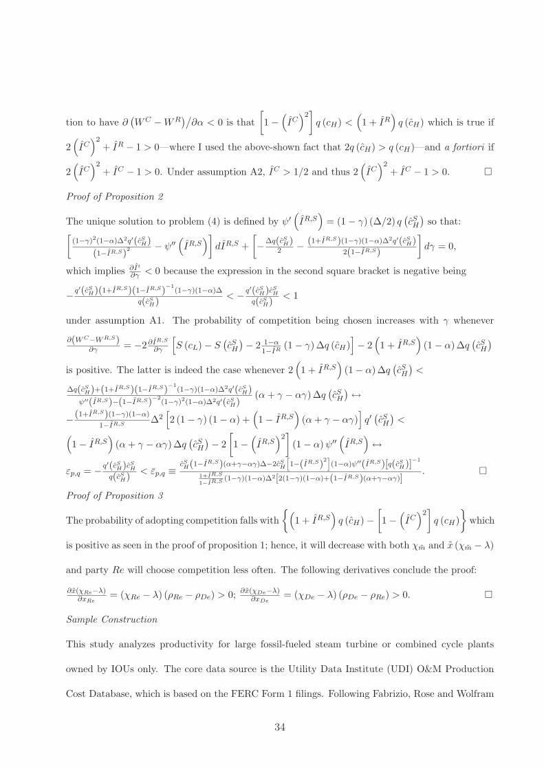
Proof of Proposition 2

The unique solution to problem (4) is defined by ψ′(

IR,S)

= (1 − γ) (∆/2) q(

cSH)

so that:[

(1−γ)2(1−α)∆2q′(cSH)

(1−IR,S)2 − ψ′′

(

IR,S)

]

dIR,S +

[

−∆q(cSH)

2 −(1+IR,S)(1−γ)(1−α)∆2q′(cSH)

2(1−IR,S)

]

dγ = 0,

which implies ∂Ii

∂γ< 0 because the expression in the second square bracket is negative being

−q′(cSH)(1+IR,S)(1−IR,S)

−1(1−γ)(1−α)∆

q(cSH)< −

q′(cSH)cSHq(cSH)

< 1

under assumption A1. The probability of competition being chosen increases with γ whenever

∂(WC−WR,S)∂γ

= −2∂IR,S

∂γ

[

S (cL) − S(

cSH)

− 2 1−α1−IR

(1 − γ)∆q (cH)]

− 2(

1 + IR,S)

(1 − α) ∆q(

cSH)

is positive. The latter is indeed the case whenever 2(

1 + IR,S)

(1 − α) ∆q(

cSH)

<

∆q(cSH)+(1+IR,S)(1−IR,S)−1

(1−γ)(1−α)∆2q′(cSH)ψ′′(IR,S)−(1−IR,S)

−2(1−γ)2(1−α)∆2q′(cSH)

(α+ γ − αγ)∆q(

cSH)

↔

−(1+IR,S)(1−γ)(1−α)

1−IR,S∆2

[

2 (1 − γ) (1 − α) +(

1 − IR,S)

(α+ γ − αγ)]

q′(

cSH)

<

(

1 − IR,S)

(α+ γ − αγ)∆q(

cSH)

− 2

[

1 −(

IR,S)2

]

(1 − α)ψ′′(

IR,S)

↔

εp,q = −q′(cSH)cSHq(cSH)

< εp,q ≡cSH(1−IR,S)(α+γ−αγ)∆−2cS

H

[

1−(IR,S)2]

(1−α)ψ′′(IR,S)[q(cSH)]−1

1+IR,S

1−IR,S (1−γ)(1−α)∆2[2(1−γ)(1−α)+(1−IR,S)(α+γ−αγ)]. �

Proof of Proposition 3

The probability of adopting competition falls with

{

(

1 + IR,S)

q (cH) −

[

1 −(

IC)2

]

q (cH)

}

which

is positive as seen in the proof of proposition 1; hence, it will decrease with both χm and x (χm − λ)

and party Re will choose competition less often. The following derivatives conclude the proof:

∂x(χRe−λ)∂xRe

= (χRe − λ) (ρRe − ρDe) > 0; ∂x(χDe−λ)∂xDe

= (χDe − λ) (ρDe − ρRe) > 0. �

Sample Construction

This study analyzes productivity for large fossil-fueled steam turbine or combined cycle plants

owned by IOUs only. The core data source is the Utility Data Institute (UDI) O&M Production

Cost Database, which is based on the FERC Form 1 filings. Following Fabrizio, Rose and Wolfram

34

(2007), I have eliminated the plants with mean capacity in gross megawatts below 100 MW or with

three years of operations at a scale not greater than 100 MW, the plants with missing or nonposi-

tive output data and the outliers spotted using the Stata’s dfbeta regression diagnostic. Moreover,

I did not consider the plants for which data on regulatory institutions and political competition

were not available: thus, there are no observations for Alaska, the District of Columbia, Nebraska,

Rhode Island, Tennessee and Vermont. Also, there are no IOUs serving Hawaii and Idaho in the

UDI Database. As a result, after imputing 46 data points using the year foregoing the missing

observation, I obtain a dataset with 8,059 observations on 503 plant-epochs—i.e., years over which

the plant capacity did not change more than 40 MW or the 15 percent of the capacity—operating in

43 U.S. states. Aggregating the plant-epochs data at the state level produces the strongly balanced

panel of 817 observations—i.e., 19 yearly data points for 43 states—used to obtain Table 2 and 3.

Data Sources

Deregulation.—Data on restructuring come from: 1. EIA (2003); 2. EIA. 2000. “The Changing

Structure of the Electric Power Industry: 2000 An Update.” EIA; 3. EIA. 2002. “Status of State

Electric Industry Restructuring Activity.” EIA; 4. Edison Electric Institute. 2001. “Electric

Competition in the States.” EEI; 5. National Association of Regulatory Utility Commissioners

(NARUC). 1995 and 1996. “Utility Regulatory Policy in the United States and Canada, Compi-

lation.” NARUC; 6. Council of State Governments (CGS). 1999. “Restructuring the Electricity

Industry.” CSG; 7. State Public Utility Commission websites, relevant legislation, and reports.

IOU operating data.—The number of employees, the total annual BTUs of fuel consumption and

net MWh generation are collected from the UDI O&M Production Cost Database.

Wages.—US Department of Labor, BLS. Electric Utility Wages: SIC Industries 4911.

composite fossil fuels price index.—Data on prices of fossil fuels reported in kilowatt hours come

from the Energy Information Administration, Annual Energy Review, 1999, Table 3.1 and are de-

35

noted in dollars per BTUs.

Appointment rules.—NARUC (1981-1999).

Political competition.—CSG. 1981-1999. The Book of the States. CSG.

References

Aghion, Philippe, Nick Bloom, Richard Blundell and Rachel Griffith. 2005. “Compe-tition and Innovation: an Inverted-U Relationship.” Quarterly Journal of Economics, 120:701-728.

Aghion, Philippe, Yann Algan, Pierre Cahuc, and Andrei Shleifer. 2010. “Regulationand Distrust.” Quarterly Journal of Economics, 125: 1015-1049.

Ai, Chunrong, and Edward C. Norton. 2003. “Interaction Terms in Logit and ProbitModels.” Economics Letters, 80: 123-129.

Alesina, Alberto, and Guido Tabellini. 1990. “A Positive Theory of Fiscal Deficits andGovernment Debt.” Review of Economic Studies, 57: 403-414.

Alesina, Alberto, Silvia Ardagna, Giuseppe Nicoletti, and Fabio Schiantarelli. 2005.“Regulation and Investment.” Journal of the European Economic Association, 3: 791-825.

Alesina, Alberto, and Guido Tabellini. 2007. “Bureaucrats or Politicians? Part I: ASingle Policy Task.” American Economic Review, 97: 169-179.

Alesina, Alberto, and Richard Holden. 2008. “Extremism and Ambiguities in Two-Candidate Elections.” NBER working paper no. 14143.

Armstrong, Mark, and David E. M. Sappington. 2006. “Regulation, Competition, andLiberalization.” Journal of Economics Literature, 44: 325-366.

Armstrong, Mark, and David E. M. Sappington. 2007. “Recent Developments in theTheory of Regulation.” in Handbook of Industrial Organization, Vol. III. Mark Armstrongand Robert Porter, eds. Amsterdam: North-Holland.

Ajodhia, Virendra, and Rudi Hakvoort. 2005. “Economic Regulation of Quality inElectricity Distribution Networks.” Utilities Policy, 13: 211-221.

Baggs, Jen, and Jean-Etienne de Bettignies. 2007. “Product Market Competition andAgency Costs.” Journal of Industrial Economics, 55: 289-323.

Baumol, William J., and Alvin K. Klevorick. 1970. “Input Choices and Rate-of-ReturnRegulation: An overview of the Discussion.” Bell Journal of Economics, 1: 289-323.

36

Belloc, Filippo, and Antonio Nicita. 2010. “Privatization-Liberalization Paths. DoesGovernment Ideology Matter?” Unpublished.

Benmelech, Efraim and Tobias J. Moskowitz. 2010. “The Political Economy of FinancialRegulation: Evidence from U.S. State Usury Laws in the 19th Century.” Journal of Finance,65: 1029-1073.

Besley, Timothy, and Stephen Coate. 2003. “Elected versus Appointed Regulators:Theory and Evidence.” Journal of the European Economic Association, 1: 1176-1206.

Boyer, Marcel, and Jean-Jacques Laffont. 2003. “Competition and the Reform of Incen-tive Schemes in the Regulated Sector.” Journal of Public Economics, 87: 1353-1381.

Bushnell, James B., and Catherine Wolfram. 2005. “Ownership Change, Incentives andPlant Efficiency: The Divesture of U.S. Generation Plants.” University of California EnergyInstitute, Working Paper, 140.

Bushnell, James B., Erin T. Mansur, and Celeste Saravia. 2008. “Vertical Arrangements,Market Structure, and Competition: An Analysis of Restructured US Electricity Markets.”American Economic Review, 98: 237-266.

Craig, J. D. and Scott J. Savage. 2010. “Market Restructuring and Productive Efficiency:Plant-level Evidence from U.S. electricity Generation.” Unpublished.

Duso, Tomaso, and Lars-Hendrik Roller. 2003. “Endogenous Deregulation: Evidencefrom OECD Countries.” Economic Letters, 81: 67-71.

EIA. 2003. “Status of State Electric Industry Restructuring Activity – as of February2003.” EIA: Washington, DC.

Espey, James A., and Molly Espey. 2004. “Turning on the Lights: A Meta-analysis ofResidential Electricity Demand Elasticities.” Journal of Agricultural and Applied Economics,36: 65-81.

Fabrizio, Kira, Nancy Rose, and Catherine Wolfram. 2007. “Do Markets Reduce Costs?Assessing the Impact of Regulatory Restructuring on U.S. Electric Generation Efficiency.”American Economic Review, 97: 1250-1277.

Faure-Grimaud, Antoine, and David Martimort. 2003. “Regulatory Inertia.” Rand

Journal of Economics, 34: 413-437.

Fremeth, Adam, and Guy L. F. Holburn. 2010. “Information Asymmetries and Regula-tory Decision Costs: Evidence from Electric Utility Rate Reviews 1980-2000.” forthcoming,Journal of Law, Economics, and Organization.

Friedman, Lee S. 1991. “Energy Utility Pricing and Customer Response.” In Regulatory

Choices: A Perspective on Developments in Energy Policy, ed. Gilber, Richard J. Universityof California Press: Berkeley, U.S.A.

37

Glaeser, Edward L., and Andrei Shleifer. 2003. “The Rise of the Regulatory State.”Journal of Economic Literature, 41: 401-425.

Glaeser, Edward L., Giacomo A. M. Ponzetto, and Jesse M. Shapiro. 2005. “Strate-gic Extremism: Why Republicans and Democrats Divide on Religious Values?” Quarterly

Journal of Economics, 120: 1283-1330.

Gormley, William T. 1983. The Politics of Public Utility Regulation. University ofPittsburgh Press: Pittsburgh, PA.

Guerriero, Carmine. 2010a. “The Political Economy of Incentive Regulation: Theoryand Evidence from the U.S. States.” Unpublished.

Guerriero, Carmine. 2010b. “Accountability in Government and Regulatory Policies:Theory and Evidence.” Unpublished.

Hanssen, Andrew F. 2004. “Is There a Politically Optimal Level of Judicial Indepen-dence?” American Economic Review, 94: 712-729.

Joskow, Paul. 1974. “Inflation and Environmental Concern: Structural Change in theProcess of Public Utility Regulation.” Journal of Law and Economics, 17: 291-327.

Joskow, Paul, and Richard Schmalansee. 1986. “Incentive Regulation for Electric Utili-ties.” Yale Journal of Regulation, 4: 1-49.

Joskow, Paul. 2008. “Lessons Learned From Electricity Market Liberalization.” Energy

Journal, 29: 9-42.

Knittel, Christopher R. 2006. “The Adoption of State Electricity Regulation: the Roleof Interest Groups.” Journal of Industrial Economics, 54: 201-222.

Laffont, Jean-Jacques, and Jean Tirole. 1993. A Theory of Incentives in Procurement

and Regulation. MIT Press: Cambridge MA.

Leaver, Clare. 2009. “Bureaucratic Minimal Squawk Behavior: Theory and Evidencefrom Regulatory Policy.” American Economic Review, 99: 572-607.

Margolis, Robert M., and Daniel M. Kammen. 1999. “Evidence of Under-investment inEnergy R&D in the United States and the Impact of Federal Policy.” Energy Policy, 27:575-584.

Metcalf, Gilbert E. 2008. “Using Tax Expenditures to Achieve Energy Policy Goals.”American Economic Review, 98: 90-94.

Myerson, Roger B. 1979. “Incentive Compatibility and the Bargaining Problem.” Econo-

metrica, 47: 61-73.

NARUC. 1981-1999. Yearbook of Regulatory Agencies. NARUC Press: Washington, DC.

38

Parker, David, Colin Kirkpatrick, and Yin-Fang Zhang. 2008. “Electricity Sector Re-form in Developing Countries: an Econometric Assessment of the Effects of Privatization,Competition and Regulation.” Journal of Regulatory Economics, 33: 159-178.

Persson, Torsten, and Lars E. O. Svensson. 1989. “Why a Stubborn Conservative WouldRun a Deficit: Policy with Time-Inconsistent Preferences.” Quarterly Journal of Economics,104: 325-345.

Pinotti, Paolo. 2010. “Trust, Regulations and Market Failures.” Unpublished.

Potrafke, Niklas. 2010. “Does Government Ideology Influence Deregulation of ProductMarkets? Empirical Evidence from OECD Countries.” Public Choice, 143: 135-155.

Raith, Michael. 2003. “Competition, Risk, and Managerial Incentives.” American Eco-

nomic Review, 93: 1425-1436.

Roodman, David M. 2009. “How to do Xtabond2: an Introduction to “Difference” and“System” GMM in Stata.” Stata Journal, 9: 86-136.

Sappington, David E. M. 1986. “Commitment to Regulatory Bureaucracy.” Information

Economics and Policy, 2: 243-258.

Shumilkina, Evgenia. 2009. “Industry Restructuring, Regulatory Reform, and the Qual-ity of Service in U.S. Electric Markets: An Interim Assessment.” Unpublished.

Steiner, Faye. 2004. “The Market Response to Restructuring: a Behavioural Model.”Journal of Regulatory Economics, 25: 59-80.

Stigler, George. 1971. “The Theory of Economic Regulation.” Bell Journal of Eco-

nomics, 2: 3-21.

Stiglitz, Joseph. 1989. Wither Socialism? Cambridge and London: MIT Press.

Teske, Paul. 2004. Regulation in the States. Brookings Institution: Washington, DC.

Vives, Xavier. 2008. “Innovation and Competitive Pressure.” Journal of Industrial

Economics, 56: 419-469.

White, Matthew W. 1996. “Power Struggles: Explaining Deregulatory Reforms in Elec-tricity Markets.” Brooking Papers on Economic Activity, Microeconomics, 67: 201-267.

Windmeijer, Frank. 2005. “A Finite Sample Correction for the Variance of LinearEfficient Two-step GMM Estimators.” Journal of Econometrics, 126: 25-51.

Zhang, Yin Fang. 2007. “Does Electricity Restructuring Work? Evidence from the U.S.Nuclear Energy Industry.” Journal of Industrial Economics, 55: 397-418.

39

Tables

Table 1: Variables Names and DescriptionsMean

Variables Variable Description (StandardName deviation)

Deregulation:1 for states that restructured or for IOU plants in states that restructured, 0.137beginning in the year of the first formal hearing; 0 otherwise. (0.344)

Market Law : 1 for states that restructured or for IOU plants in states that restructured, 0.055institutions: beginning in the year in which legislation was enacted; 0 otherwise. (0.228)

Der Ord : Indicator equal to: 3 when both Deregulation and Law are equal to 1; 2 when 1.192only Deregulation equals 1; 1 otherwise. (0.515)

Mc Labor : Average marginal labor cost in cents of dollar per Kwh calculated at the state 0.570level. At the plant level, it is obtained dividing the product of the number of (1.688)employees and their annual wage bill by the total generation.

Mc Fuel : Average marginal fuel cost in cents of dollar per Kwh calculated at the state 1.889level. At the plant level, it is obtained dividing the product of total BTUs (1.407)and the composite fossil fuels price index by the total generation.

Heat Rate: Average heat rate calculated at the state level. At the plant level, the heat 9.523rate measures the BTUs necessary to produce 1 MWh of power. (2.550)

Marginal Ratio Mlc: Ratio of the average marginal labor cost in a state over those of bordering 1.530costs, states. (4.640)inefficiency Ratio Mfc: Ratio of the average marginal fuel cost in a state over those of bordering 1.051measures and states. (0.722)input uses: Ratio Hr : Ratio of the average heat rate in a state over those of bordering states. 1.037

(0.476)Ln Emp: ln (annual average number of employees). 4.745

(0.804)Ln Btu: ln (total BTUs of fuel consumption). Total BTUs are calculated as: 30.577

(tons of coal*2000 lbs/ton*BTU/lb) + (barrels of oil*42 gal/barrel*BTU/gal) + (1.282)(Mcf gas*1000 cf/mcf*BTU/cf).

Ln Hr : ln (heat rate in BTUs per MW). 2.388(0.223)

Supervision Elec Reg: 1 for states or for IOU plants in a state where the public utility commissioners 0.215technology: are elected; 0 otherwise. (0.411)

Republican: 1 for states or for IOU plants in a state where both houses are controlled with 0.258Political the relative majority of seats by the Republican party; 0 otherwise. (0.438)competition: Majority: Share of seats held by the majority party averaged across both houses. The 0.542

variable equals 0 when no party holds the relative majority in both houses. (0.283)Ln Mwhs: ln (annual net MWh generation). 14.374

(1.369)Ln Wage: ln (Bureau of Labor Statistics annual wage bill in dollars divided by total 10.576

Other employment calculated at the state-year level for IOU plants). (0.277)controls: Scrubber : 1 for IOU plants having a FGD scrubber; 0 otherwise. 0.096

(0.295)Der Nei : Share of bordering states for which Deregulation equals 1. 0.141

(0.278)Note : 1. All the statistics are computed for the full sample 1981-1999 and across states except in the cases of Ln Emp, Ln Btu, Ln Hr,

Ln Mwhs, Ln Wage and Scrubber, which are computed across plants.

40

Table 2: Determinants of Deregulation — Ordered Logit(1) (2) (3) (4) (5) (6)

The dependent variable is Der Ord

Mc Labor(-3) 0.881(0.200)

Mc Fuel(-3) 0.256(0.078)***

Heat Rate(-3) 0.931(0.052)

Ratio Mlc(-3) 0.931(0.083)

Ratio Mfc(-3) 0.338(0.174)**

Ratio Hr(-3) 0.702(0.320)

Elec Reg 1.324 1.155 1.362 1.317 1.300 1.360(0.496) (0.445) (0.505) (0.489) (0.482) (0.503)

Republican 1.313 1.201 1.282 1.307 1.255 1.275(0.407) (0.378) (0.404) (0.402) (0.396) (0.399)

Majority 0.461 0.538 0.466 0.476 0.450 0.441(0.212)* (0.240) (0.207)* (0.224) (0.198)* (0.198)*

Der Nei 322.495 201.726 300.483 322.2 340.210 311.076(146.318)*** (91.439)*** (134.476)*** (146.14)*** (155.599)*** (136.760)***

Pseudo R2 0.37 0.39 0.38 0.37 0.38 0.37Log Pseudo-likelihood - 238.44 - 231.02 - 237.73 - 238.24 - 236.38 - 238.38Number ofObservations 688 688 688 688 688 688Notes: 1. The unit of observation is state per year;

2. The entries are odds ratios;3. In parentheses are reported the robust standard errors;4. *** denotes significant at the 1% confidence level; **, 5%; *, 10%.

Table 3: Determinants of Deregulation — Logit(1) (2) (3) (4) (5) (6)

The dependent variable is the likelihood of Deregulation

Elec Reg 0.015 - 0.001 0.011 0.015 0.009 0.008(0.028) (0.017) (0.026) (0.027) (0.024) (0.023)

Mc Labor(-3) - 0.007(0.016)

Mc Fuel(-3) - 0.082(0.013)***

Heat Rate(-3) - 0.013(0.004)***

Ratio Mlc(-3) - 0.004(0.007)

Ratio Mfc(-3) - 0.105(0.034)***

Ratio Hr(-3) - 0.130(0.031)***

Republican 0.035 0.018 0.030 0.034 0.027 0.024(0.029) (0.020) (0.028) (0.029) (0.027) (0.025)

Majority - 0.077 - 0.038 - 0.065 - 0.075 - 0.069 - 0.066(0.037)** (0.027) (0.037)* (0.038)** (0.035)** (0.033)**

Der Nei 0.414 0.256 0.401 0.411 0.392 0.372(0.051)*** (0.047)*** (0.052)*** (0.052)*** (0.051)*** (0.053)***

Pseudo R2 0.45 0.48 0.46 0.45 0.46 0.47Log Pseudo-likelihood - 169.29 - 159.60 - 165.56 - 169.18 - 165.58 - 163.42Number ofObservations 688 688 688 688 688 688Notes: 1. The unit of observation is state per year;

2. The entries are marginal effects;3. In parentheses are reported the robust standard errors;4. *** denotes significant at the 1% confidence level; **, 5%; *, 10%.

41

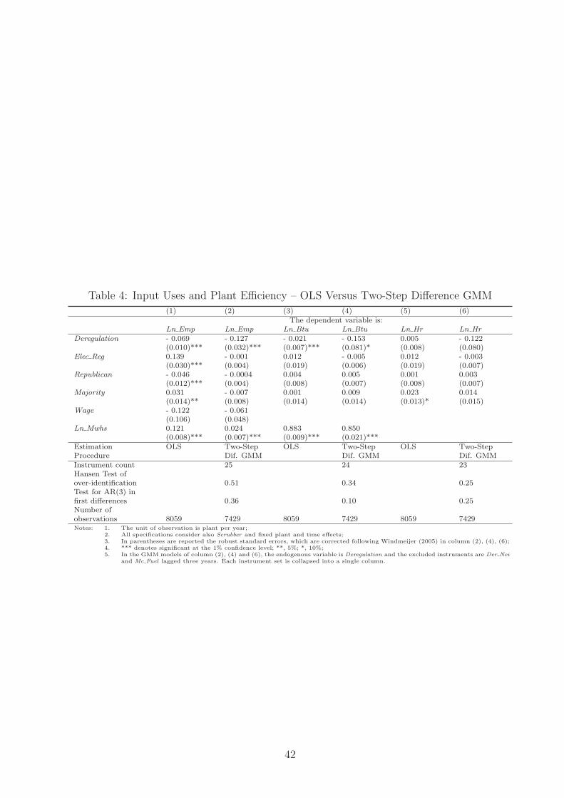
Table 4: Input Uses and Plant Efficiency – OLS Versus Two-Step Difference GMM(1) (2) (3) (4) (5) (6)

The dependent variable is:Ln Emp Ln Emp Ln Btu Ln Btu Ln Hr Ln Hr

Deregulation - 0.069 - 0.127 - 0.021 - 0.153 0.005 - 0.122(0.010)*** (0.032)*** (0.007)*** (0.081)* (0.008) (0.080)

Elec Reg 0.139 - 0.001 0.012 - 0.005 0.012 - 0.003(0.030)*** (0.004) (0.019) (0.006) (0.019) (0.007)

Republican - 0.046 - 0.0004 0.004 0.005 0.001 0.003(0.012)*** (0.004) (0.008) (0.007) (0.008) (0.007)

Majority 0.031 - 0.007 0.001 0.009 0.023 0.014(0.014)** (0.008) (0.014) (0.014) (0.013)* (0.015)

Wage - 0.122 - 0.061(0.106) (0.048)

Ln Mwhs 0.121 0.024 0.883 0.850(0.008)*** (0.007)*** (0.009)*** (0.021)***

Estimation OLS Two-Step OLS Two-Step OLS Two-StepProcedure Dif. GMM Dif. GMM Dif. GMMInstrument count 25 24 23Hansen Test ofover-identification 0.51 0.34 0.25Test for AR(3) infirst differences 0.36 0.10 0.25Number ofobservations 8059 7429 8059 7429 8059 7429Notes: 1. The unit of observation is plant per year;

2. All specifications consider also Scrubber and fixed plant and time effects;3. In parentheses are reported the robust standard errors, which are corrected following Windmeijer (2005) in column (2), (4), (6);4. *** denotes significant at the 1% confidence level; **, 5%; *, 10%;5. In the GMM models of column (2), (4) and (6), the endogenous variable is Deregulation and the excluded instruments are Der Nei

and Mc Fuel lagged three years. Each instrument set is collapsed into a single column.

42