Embed Size (px)
Citation preview

The Poincaré - Birkhoff theorem in theframework of Hamiltonian systems
Alessandro Fonda
(Università degli Studi di Trieste)
a collaboration with Antonio J. Ureña

The Poincaré - Birkhoff theorem in theframework of Hamiltonian systems
Alessandro Fonda
(Università degli Studi di Trieste)
a collaboration with Antonio J. Ureña

Jules Henri Poincaré (1854 – 1912)


Poincaré’s“Théorème de géométrie”
A is a closed planar annulus
P : A → A is an area preserving homeomorphism
and
(?) it rotates the two boundary circles in opposite directions
(this is called the “twist condition”).

Poincaré’s“Théorème de géométrie”
A is a closed planar annulus
P : A → A is an area preserving homeomorphism
and
(?) it rotates the two boundary circles in opposite directions
(this is called the “twist condition”).

Poincaré’s“Théorème de géométrie”
A is a closed planar annulus
P : A → A is an area preserving homeomorphism
and
(?) it rotates the two boundary circles in opposite directions
(this is called the “twist condition”).

Poincaré’s“Théorème de géométrie”
A is a closed planar annulus
P : A → A is an area preserving homeomorphism
and
(?) it rotates the two boundary circles in opposite directions
(this is called the “twist condition”).

Poincaré’s“Théorème de géométrie”
A is a closed planar annulus
P : A → A is an area preserving homeomorphism
and
(?) it rotates the two boundary circles in opposite directions
(this is called the “twist condition”).

Poincaré’s“Théorème de géométrie”
A is a closed planar annulus
P : A → A is an area preserving homeomorphism
and
(?) it rotates the two boundary circles in opposite directions
(this is called the “twist condition”).

Poincaré’s“Théorème de géométrie”
A is a closed planar annulus
P : A → A is an area preserving homeomorphism
and
(?) it rotates the two boundary circles in opposite directions
(this is called the “twist condition”).
Then, P has two fixed points.

Poincaré’s“Théorème de géométrie”
A is a closed planar annulus
P : A → A is an area preserving homeomorphism
and
(?) it rotates the two boundary circles in opposite directions
(this is called the “twist condition”).
Then, P has two fixed points.

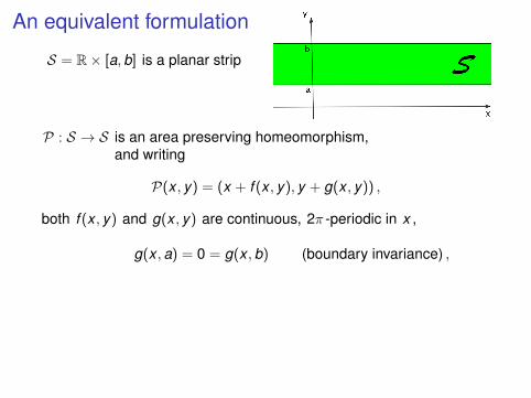
An equivalent formulation
S = R× [a,b] is a planar strip
P : S → S is an area preserving homeomorphism,and writing
P(x , y) = (x + f (x , y), y + g(x , y)) ,
both f (x , y) and g(x , y) are continuous, 2π -periodic in x ,
g(x ,a) = 0 = g(x ,b) (boundary invariance) ,
and
(?) f (x ,a) < 0 < f (x ,b) (twist condition) .

An equivalent formulation
S = R× [a,b] is a planar strip
P : S → S is an area preserving homeomorphism
,and writing
P(x , y) = (x + f (x , y), y + g(x , y)) ,
both f (x , y) and g(x , y) are continuous, 2π -periodic in x ,
g(x ,a) = 0 = g(x ,b) (boundary invariance) ,
and
(?) f (x ,a) < 0 < f (x ,b) (twist condition) .

An equivalent formulation
S = R× [a,b] is a planar strip
P : S → S is an area preserving homeomorphism,and writing
P(x , y) = (x + f (x , y), y + g(x , y)) ,
both f (x , y) and g(x , y) are continuous, 2π -periodic in x ,
g(x ,a) = 0 = g(x ,b) (boundary invariance) ,
and
(?) f (x ,a) < 0 < f (x ,b) (twist condition) .

An equivalent formulation
S = R× [a,b] is a planar strip
P : S → S is an area preserving homeomorphism,and writing
P(x , y) = (x + f (x , y), y + g(x , y)) ,
both f (x , y) and g(x , y) are continuous, 2π -periodic in x ,
g(x ,a) = 0 = g(x ,b) (boundary invariance) ,
and
(?) f (x ,a) < 0 < f (x ,b) (twist condition) .
Then, P has two geometrically distinct fixed points.

George David Birkhoff (1884 – 1944)

The Poincaré – Birkhoff theorem
In 1913 – 1925, Birkhoff proved Poincaré’s “théorème de géométrie”,so that it now carries the name
“Poincaré – Birkhoff Theorem”.
Variants and different proofs have been proposed by:
Brown–Neumann, Carter, W.-Y. Ding, Franks, Guillou, Jacobowitz, deKérékjartó, Le Calvez, Moser, Rebelo, Slaminka, ...
Applications to the existence of periodic solutions were provided by:
Bonheure, Boscaggin, Butler, Corsato, Del Pino, T. Ding, Fabry,Garrione, Hartman, Manásevich, Mawhin, Omari, Ortega, Sabatini,Sfecci, Smets, Torres, Zanini, Zanolin, ...

Periodic solutions as fixed points of the Poincaré map
We consider the system
x =∂H∂y
(t , x , y) , y = −∂H∂x
(t , x , y) ,
and assume that the Hamiltonian H(t , x , y) is T -periodic in t .
The Poincaré time – map is defined as
P : (x0, y0) 7→ (xT , yT )
i.e.
to each “starting point” (x0, y0) of a solution at time t = 0,
P associates
the “arrival point” (xT , yT ) of the solution at time t = T .

Good and bad news
We consider the system
x =∂H∂y
(t , x , y) , y = −∂H∂x
(t , x , y) ,
and assume that the Hamiltonian H(t , x , y) is T -periodic in t .
Good news:
The Poincaré map P is an area preserving homeomorphism.
Its fixed points correspond to T -periodic solutions.
Bad news:
It is very difficult to find an invariant annulus for P .

Generalizing the Poincaré – Birkhoff theorem(in the framework of Hamiltonian systems)
We consider the system
x =∂H∂y
(t , x , y) , y = −∂H∂x
(t , x , y) ,
and assume that the Hamiltonian H(t , x , y) is T -periodic in t .
Assume H(t , x , y) to be also 2π -periodic in x .
Let S = R× [a,b] be a planar strip.
Twist condition: the solutions (x(t), y(t)) with “starting point”(x(0), y(0)) on ∂S are defined on [0,T ] and satisfy
(?) x(T )− x(0)
{< 0 , if y(0) = a ,> 0 , if y(0) = b .
Then, there are two geometrically distinct T -periodic solutions.

The twist condition
Writing S = R×D , withD = ]a,b[ ,
and defining the “outer normal function” ν : ∂D → R as
ν(a) = −1 , ν(b) = +1 ,
the twist condition
(?) (x(0), y(0)) ∈ ∂S ⇒ x(T )− x(0)
{< 0 , if y(0) = a ,> 0 , if y(0) = b ,
can be written as
(?) (x(0), y(0)) ∈ ∂S ⇒ [x(T )− x(0)] · ν(y(0)) > 0 .

A higher dimensional version of the theorem
We now discuss about
the outstanding question as to the possibility of an N -dimensionalextension of Poincaré’s last geometric theorem
[Birkhoff, Acta Mathematica 1925]
Attempts in some directions have been made by:
Amann, Bertotti, Birkhoff, K.C. Chang, Conley, Felmer, Fournier,Golé, Hingston, Josellis, J.Q. Liu, Lupo, Mawhin, Moser, Rabinowitz,Ramos, Szulkin, Weinstein, Willem, Winkelnkemper, Zehnder, ...
However,a genuine generalization of the Poincaré – Birkhoff theorem
to higher dimensions has never been given.
[Moser and Zehnder, Notes on Dynamical Systems, 2005].

A higher dimensional version of the theorem
We consider the system
x =∂H∂y
(t , x , y) , y = −∂H∂x
(t , x , y) ,
and assume that the Hamiltonian H(t , x , y) is T -periodic in t .
Here, x = (x1, . . . , xN) and y = (y1, . . . , yN) .
Assume H(t , x , y) to be also 2π -periodic in each x1, . . . , xN .
Let D be an open, bounded, convex set in RN , with a smoothboundary, and denote by ν : ∂D → RN the outward normalvectorfield.
Consider the “strip” S = RN ×D .
Twist condition: for a solution (x(t), y(t)) ,
(?) (x(0), y(0)) ∈ ∂S ⇒ [x(T )− x(0)]·ν(y(0)) > 0 .
(this is the old condition)

A higher dimensional version of the theorem
We consider the system
x =∂H∂y
(t , x , y) , y = −∂H∂x
(t , x , y) ,
and assume that the Hamiltonian H(t , x , y) is T -periodic in t .
Here, x = (x1, . . . , xN) and y = (y1, . . . , yN) .
Assume H(t , x , y) to be also 2π -periodic in each x1, . . . , xN .
Let D be an open, bounded, convex set in RN , with a smoothboundary, and denote by ν : ∂D → RN the outward normalvectorfield. Consider the “strip” S = RN ×D .
Twist condition: for a solution (x(t), y(t)) ,
(?) (x(0), y(0)) ∈ ∂S ⇒⟨x(T )− x(0) , ν(y(0))
⟩> 0 .
(this is the new condition)

A higher dimensional version of the theorem
We consider the system
x =∂H∂y
(t , x , y) , y = −∂H∂x
(t , x , y) ,
and assume that the Hamiltonian H(t , x , y) is T -periodic in t .
Here, x = (x1, . . . , xN) and y = (y1, . . . , yN) .
Assume H(t , x , y) to be also 2π -periodic in each x1, . . . , xN .
Let D be an open, bounded, convex set in RN , with a smoothboundary, and denote by ν : ∂D → RN the outward normalvectorfield. Consider the “strip” S = RN ×D .
Twist condition: for a solution (x(t), y(t)) ,
(?) (x(0), y(0)) ∈ ∂S ⇒⟨x(T )− x(0) , ν(y(0))
⟩> 0 .
Then, there are N + 1 geometrically distinct T -periodic solutions.

Why N + 1 solutions?
The proof is variational, it uses an
infinite dimensional Ljusternik – Schnirelmann theory
for the action functional
ϕ(x , y) = 12
∫ T
0
(〈x , y〉 − 〈x , y〉
)+
∫ T
0H(t , x(t), y(t)) dt .
Writing x(t) = x + x(t) , the periodicity in x1, . . . , xN permits to definethe action on the product of the N -torus TN and a Hilbert space E :
x ∈ TN , (x , y) ∈ E , ϕ : TN × E → R .
The result then follows from the fact that
cat(TN) = N + 1 .
Note. If ϕ only has nondegenerate critical points, then we can useMorse theory and find 2N solutions. Indeed,
sb(TN) = 2N .

Why N + 1 solutions?The proof is variational, it uses an
infinite dimensional Ljusternik – Schnirelmann theory
for the action functional
ϕ(x , y) = 12
∫ T
0
(〈x , y〉 − 〈x , y〉
)+
∫ T
0H(t , x(t), y(t)) dt .
Writing x(t) = x + x(t) , the periodicity in x1, . . . , xN permits to definethe action on the product of the N -torus TN and a Hilbert space E :
x ∈ TN , (x , y) ∈ E , ϕ : TN × E → R .
The result then follows from the fact that
cat(TN) = N + 1 .
Note. If ϕ only has nondegenerate critical points, then we can useMorse theory and find 2N solutions.
Indeed,
sb(TN) = 2N .

Why N + 1 solutions?The proof is variational, it uses an
infinite dimensional Ljusternik – Schnirelmann theory
for the action functional
ϕ(x , y) = 12
∫ T
0
(〈x , y〉 − 〈x , y〉
)+
∫ T
0H(t , x(t), y(t)) dt .
Writing x(t) = x + x(t) , the periodicity in x1, . . . , xN permits to definethe action on the product of the N -torus TN and a Hilbert space E :
x ∈ TN , (x , y) ∈ E , ϕ : TN × E → R .
The result then follows from the fact that
cat(TN) = N + 1 .
Note. If ϕ only has nondegenerate critical points, then we can useMorse theory and find 2N solutions. Indeed,
sb(TN) = 2N .

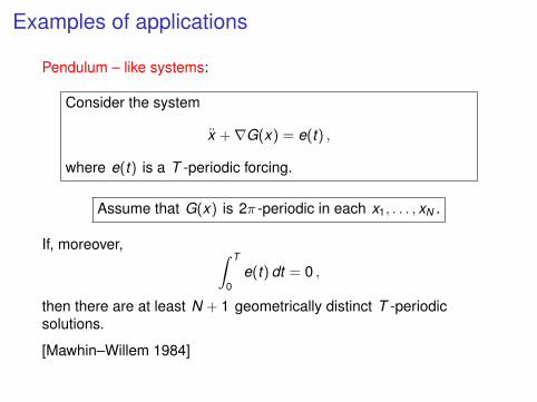
Examples of applications
Pendulum – like systems:
Consider the system
x +∇G(x) = e(t) ,
where e(t) is a T -periodic forcing.
Assume that G(x) is 2π -periodic in each x1, . . . , xN .
If, moreover, ∫ T
0e(t) dt = 0 ,
then there are at least N + 1 geometrically distinct T -periodicsolutions.
[Mawhin–Willem 1984]

Examples of applications
Superlinear systems:
Consider a system of the typex1 + g1(x1) =
∂U∂x1
(t , x1, . . . , xN) ,
. . .
xN + gN(xN) =∂U∂xN
(t , x1, . . . , xN) ,
where all∂U∂xk
(t , x1, . . . , xN) are bounded, and T -periodic in t .
Assume that, for every k ,
lim|ξ|→∞
gk (ξ)
ξ= +∞ .
Then, there are infinitely many T -periodic solutions.
[Ding–Zanolin 1992, Boscaggin–Ortega 2014]

Examples of applicationsSuperlinear systems:
Consider a system of the typex1 + g1(x1) =
∂U∂x1
(t , x1, . . . , xN) ,
. . .
xN + gN(xN) =∂U∂xN
(t , x1, . . . , xN) ,
where all∂U∂xk
(t , x1, . . . , xN) are bounded, and T -periodic in t .
Assume that, for every k ,
lim|ξ|→∞
gk (ξ)
ξ= +∞ .
Then, there are infinitely many T -periodic solutions.
[Ding–Zanolin 1992, Boscaggin–Ortega 2014]

Examples of applications
Superlinear systems:
Consider a Hamiltonian system of the type−x1 = x1
[h1(t , x1) + e1(t , x1, . . . , xN)
],
. . .
−xN = xN
[hN(t , xN) + eN(t , x1, . . . , xN)
],
where all ek (t , x1, . . . , xN) are bounded, and T -periodic in t .
Assume that, for every k ,
lim|ξ|→∞
hk (t , ξ) = +∞ .
Then, there are infinitely many T -periodic solutions.
[Jacobowitz 1976, Hartman 1977, F.–Sfecci 2014]

More general twist conditions
The twist condition
(?) (x(0), y(0)) ∈ ∂S ⇒⟨x(T )− x(0) , ν(y(0))
⟩> 0
can be improved in two directions.
I. The “indefinite twist” condition:for a regular symmetric N × N matrix A ,
(?′) (x(0), y(0)) ∈ ∂S ⇒⟨x(T )− x(0) ,Aν(y(0))
⟩> 0 .
II. The “avoiding rays” condition:
(?′′) (x(0), y(0)) ∈ ∂S ⇒ x(T )− x(0) /∈ {−λν(y(0)) : λ ≥ 0} .

More general twist conditions
II. The “avoiding rays” condition:
(?′′) (x(0), y(0)) ∈ ∂S ⇒ x(T )− x(0) /∈ {−λν(y(0)) : λ ≥ 0} .

More general twist conditions
II. The “avoiding rays” condition:
(?′′) (x(0), y(0)) ∈ ∂S ⇒ x(T )− x(0) /∈ {−λν(y(0)) : λ ≥ 0} .

a collaboration with Antonio J. Ureña


![arXiv:math/9908139v2 [math.HO] 27 Apr 2000arXiv:math/9908139v2 [math.HO] 27 Apr 2000 POINCARE’S PROOF OF THE SO-CALLED´ BIRKHOFF-WITT THEOREM Tuong Ton-That Thai-Duong Tran Department](https://img.dokumen.tips/doc/110x75/5e872c982230ed5d5d0d7079/arxivmath9908139v2-mathho-27-apr-2000-arxivmath9908139v2-mathho-27-apr.jpg)


![PLANETARY BIRKHOFF NORMAL FORMS · PLANETARY BIRKHOFF NORMAL FORMS 625 below. On the reduced phase spaces, one can construct Birkhoff normal forms ([6, Sect 7 and 9]; §2, §5.1below)](https://img.dokumen.tips/doc/110x75/6047d6bd37fe306c735bee69/planetary-birkhoff-normal-planetary-birkhoff-normal-forms-625-below-on-the-reduced.jpg)


![POINCARE-BIRKHOFF-WITT THEOREMSsjw/pub/PBW-survey.pdf · POINCARE-BIRKHOFF-WITT THEOREMS 5 a sum of larger elements in the basis. In doing so, Priddy [79, Theorem 5.3] gave a class](https://img.dokumen.tips/doc/110x75/5ec53bda36a8de56742843ce/poincare-birkhoff-witt-theorems-sjwpubpbw-poincare-birkhoff-witt-theorems.jpg)


