The Plug-In Hybrid Electric VehicleRouting Problem with Time

Windows

by

Tarek Abdallah

A thesispresented to the University of Waterloo

in fulfillment of thethesis requirement for the degree of

Master of Applied Sciencein

Management Sciences

Waterloo, Ontario, Canada, 2013

c© Tarek Abdallah 2013

brought to you by COREView metadata, citation and similar papers at core.ac.uk

provided by University of Waterloo's Institutional Repository

I hereby declare that I am the sole author of this thesis. This is a true copy of the thesis,including any required final revisions, as accepted by my examiners.

I understand that my thesis may be made electronically available to the public.

ii

Abstract

There is an increasing interest in sustainability and a growing debate about environmen-tal policy measures aiming at the reduction of green house gas emissions across differenteconomic sectors worldwide. The transportation sector is one major greenhouse gas emit-ter which is heavily regulated to reduce its dependance on oil. These regulations alongwith the growing customer awareness about global warming has led vehicle manufacturersto seek different technologies to improve vehicle efficiencies and reduce the green housegases emissions while at the same time meeting customer’s expectation of mobility andflexibility. Plug-in hybrid electric vehicles (PHEV) is one major promising solution for asmooth transition from oil dependent transportation sector to a clean electric based sectorwhile not compromising the mobility and flexibility of the drivers.

In the medium term, plug-in hybrid electric vehicles (PHEV) can lead to significantreductions in transportation emissions. These vehicles are equipped with a larger batterythan regular hybrid electric vehicles which can be recharged from the grid. For shorttrips, the PHEV can depend solely on the electric engine while for longer journeys thealternative fuel can assist the electric engine to achieve extended ranges. This is beneficialwhen the use pattern is mixed such that and short long distances needs to be covered.The plug-in hybrid electric vehicles are well-suited for logistics since they can avoid thepossible disruption caused by charge depletion in case of all-electric vehicles with tighttime schedules.

The use of electricity and fuel gives rise to a new variant of the classical vehicle routingwith time windows which we call the plug-in hybrid electric vehicle routing problem withtime windows (PHEVRPTW). The objective of the PHEVRPTW is to minimize the rout-ing costs of a fleet of PHEVs by minimizing the time they run on gasoline while meeting thedemand during the available time windows. As a result, the driver of the PHEV has twodecisions to make at each node: (1) recharge the vehicle battery to achieve a longer rangeusing electricity, or (2) continue to the next open time window with the option of usingthe alternative fuel. In this thesis, we present a mathematical formulation for the plug-inhybrid-electric vehicle routing problem with time windows. We solve this problem using aLagrangian relaxation and we propose a new tabu search algorithm. We also present thefirst results for the full adapted Solomon instances.

iii

Acknowledgements

I would like to thank professor Samir Elhedhli for his continuous guidance and supportas my advisor. I would like to also thank professors Osman Ozaltin and Fatih Safa Erenayfor agreeing be on the reading committee for this thesis.

iv

Dedication

This thesis would not have been possible without the support of my family, friends,and professors.

v

Table of Contents

List of Tables viii

List of Figures ix

1 Introduction 1

1.1 Available Technologies . . . . . . . . . . . . . . . . . . . . . . . . . . . . . 2

1.1.1 Internal Combustion Engine Vehicles . . . . . . . . . . . . . . . . . 2

1.1.2 ICE Vehicles with Biofuels . . . . . . . . . . . . . . . . . . . . . . . 2

1.1.3 Electric Vehicles . . . . . . . . . . . . . . . . . . . . . . . . . . . . . 3

1.1.4 Hybrid Electric Vehicles . . . . . . . . . . . . . . . . . . . . . . . . 4

1.2 Technology Assessment . . . . . . . . . . . . . . . . . . . . . . . . . . . . . 5

1.3 Current Practices . . . . . . . . . . . . . . . . . . . . . . . . . . . . . . . . 5

1.3.1 Lean Distribution Systems . . . . . . . . . . . . . . . . . . . . . . . 6

1.4 The Plug-in Hybrid-Electric Vehicle Routing Problem . . . . . . . . . . . . 6

2 Formulation and Lagrangian Relaxations 9

2.1 Literature Review . . . . . . . . . . . . . . . . . . . . . . . . . . . . . . . . 12

2.2 The Model . . . . . . . . . . . . . . . . . . . . . . . . . . . . . . . . . . . . 15

2.3 Problem Formulation . . . . . . . . . . . . . . . . . . . . . . . . . . . . . . 16

2.3.1 Original Problem Formulation . . . . . . . . . . . . . . . . . . . . . 17

2.4 Lagrangian Relaxation . . . . . . . . . . . . . . . . . . . . . . . . . . . . . 18

vi

2.4.1 Relaxation 1 (LR1) . . . . . . . . . . . . . . . . . . . . . . . . . . . 18

2.4.2 Relaxation 2 (LR2) . . . . . . . . . . . . . . . . . . . . . . . . . . . 22

2.4.3 Relaxation 3 (LR3) . . . . . . . . . . . . . . . . . . . . . . . . . . . 25

2.5 Heuristics for Obtaining an Upper Bound . . . . . . . . . . . . . . . . . . . 30

2.6 Computational Results . . . . . . . . . . . . . . . . . . . . . . . . . . . . . 31

2.6.1 Solomon’s Instances . . . . . . . . . . . . . . . . . . . . . . . . . . . 31

2.6.2 PHEVRPTW additional Parameters . . . . . . . . . . . . . . . . . 32

2.6.3 Lower Bound Comparison . . . . . . . . . . . . . . . . . . . . . . . 32

2.6.4 LR1 v.s. Cplex . . . . . . . . . . . . . . . . . . . . . . . . . . . . . 33

2.6.5 LR1 Complete Results . . . . . . . . . . . . . . . . . . . . . . . . . 34

2.7 Conclusion . . . . . . . . . . . . . . . . . . . . . . . . . . . . . . . . . . . . 34

3 Tabu Search Algorithm 37

3.1 Literature Review . . . . . . . . . . . . . . . . . . . . . . . . . . . . . . . . 38

3.2 Algorithm Description . . . . . . . . . . . . . . . . . . . . . . . . . . . . . 41

3.2.1 Overall Framework for the Tabu Search . . . . . . . . . . . . . . . . 42

3.2.2 Initialization . . . . . . . . . . . . . . . . . . . . . . . . . . . . . . . 43

3.2.3 Neighborhood Generation . . . . . . . . . . . . . . . . . . . . . . . 46

3.2.4 Cost Evaluation Function . . . . . . . . . . . . . . . . . . . . . . . 47

3.2.5 The Tabu List and Aspiration Criteria . . . . . . . . . . . . . . . . 50

3.2.6 Diversification Strategy . . . . . . . . . . . . . . . . . . . . . . . . . 50

3.3 Computational Results . . . . . . . . . . . . . . . . . . . . . . . . . . . . . 51

3.3.1 Comparison Tabu vs. Lagrangian Relaxation . . . . . . . . . . . . . 52

3.3.2 Tabu Search Results for the 100 Customers Datasets . . . . . . . . 52

3.4 Conclusion . . . . . . . . . . . . . . . . . . . . . . . . . . . . . . . . . . . . 52

4 Conclusion 58

References 60

vii

List of Tables

2.1 Comparison of the Lagrangian bounds obtained by 3 relaxations . . . . . . 33

2.2 Computational Results using 16 nodes of some Solomon instances . . . . . 34

2.3 LR1 Results on Solomon instances 16-30 nodes . . . . . . . . . . . . . . . . 35

3.1 Comparison between the Lagrangian relaxation bound and the tabu search 53

3.2 Tabu search results for R1xx datasets with 100 nodes . . . . . . . . . . . . 54

3.3 Tabu search results for R2xx datasets with 100 nodes . . . . . . . . . . . . 54

3.4 Tabu search results for C1xx datasets with 100 nodes . . . . . . . . . . . . 55

3.5 Tabu search results for C2xx datasets with 100 nodes . . . . . . . . . . . . 55

3.6 Tabu search results for RC1xx datasets with 100 nodes . . . . . . . . . . . 56

3.7 Tabu search results for RC2xx datasets with 100 nodes . . . . . . . . . . . 56

viii

List of Figures

2.1 Illustrative Network . . . . . . . . . . . . . . . . . . . . . . . . . . . . . . . 11

ix

Chapter 1

Introduction

Over the past 50 years, logistics has played a fundamental role in the economic developmentof societies. During this period, logistics was governed by a profit maximizing paradigmthat ignored social and environmental costs. As the debate over sustainability increases,the main focus of logistics is shifting towards reducing the environmental impact of freighttransport by improving the efficiency of the vehicles and reducing the dependance on oil.

The logistics sector faces a challenging future due to its crucial and growing role in theworld energy use and green house gas (GHG) emissions. In 2004, the transport energyuse amounted to 26% of the total world energy consumption and the transport sector wasresponsible for about 23% of world energy-related GHG emissions [Birol, 2007]. The growthrate of energy consumption in the transport sector in the past decade was highest amongall the end-use sectors. Freight transport, among all sectors in the IEA-11 countries,showed the highest relative growth in CO2 emissions percentage since 1973. Emissionsincreased as freight activity grew in line with GDP and with energy-intensive truckingtaking a larger share of total ton-kilometers hauled [IEA, 2006]. Freight transport nowconsumes 35% of all transport energy, or 27 exajoules (out of 77 EJ total) with domesticfreight gaining an increasing share of the market [WBCSD, 2004]. Domestic freight, inmost of the developed countries, is dominated by road transport and is characterized bylong traveling distances and overhauls Tester [2005]. The environmental impact of freighttransport is thus determined by the efficiency of the road freight sector.

The transition to sustainable transportation is an essential step towards meeting theglobal emissions reduction targets. With the available breed of new technologies, thissector is radically changing the designs and components of the vehicles from fossil fuelbased internal combustion engine (ICE) vehicles to electric and hybrid electric vehicles.

1

This technology shift will lead to the emergence of new technology strategies that willaffect logistics sector traditional management approaches.

Proponents of renewable energy have created too many alternatives for the carbonintensive transportation; this bewildering collection of green mobility technology leaves avery simple question unanswered: Which technology is the best?

1.1 Available Technologies

Many technological improvements have been made to vehicles to reduce their environmentalimpact. Some of these advances have been imposed by environmental legislation, othershave been incentivized by commercial pressure to improve energy efficiency and adhereto the growing environmental conscious customer base. We focus our discussion on fourmain categories: internal combustion engine vehicles using fossil fuels and biofuels, electricvehicles, and hybrid electric vehicles.

1.1.1 Internal Combustion Engine Vehicles

The internal combustion engine (ICE) vehicles have dominated the transportation marketsoon after the introduction of Henry Ford’s T-model car in 1908 [Womack et al., 1991].Since then, the ICE vehicles have reached maturity after receiving of almost a century ofdedicated R&D support. Most of the current ICE vehicles run on petroleum fuel whichresults in high GHG emissions. Improving the efficiency of the ICEs can lead to substantialdecrease in GHG emissions on the short term.

As the available fossil fuel resources grow thinner, the attention is shifting to focuson developing alternative fuels, to reduce the dependence on fossil fuels. We restrict ourdiscussion to biofuels.

1.1.2 ICE Vehicles with Biofuels

These vehicles run on biofuels instead of fossil fuels. Biofuels are normally extracted fromrenewable plant materials and oils, and are mainly two types:

• Biodiesel

2

• Bioethanol

Biodiesel fuels (known as alkyl esters) are extracted from plant and animal oils througha process called “transesterification”. The level and quality of the extracted oils vary highlyfrom one country to another, depending on the local growing conditions. On the otherhand, Bioethanol fuels are extracted from biological feedstock which contain sugar. Bothfuels are usually mixed with existing fossil fuels to make them usable [Mckinnon et al.,2010].

As for their environmental effect, several research claim that significant decrease inthe major GHG emissions can be achieved by using ICE vehicles with biofuels [Demirbas,2007], [Demirbas, 2008]. However, an EPA report states that they were not able to identifyan “unambiguous” difference in exhaust CO2 emissions level [EPA, 2002].

The major criticism regarding the use of biofuels in transportation is the adverse changein the land use and deforestation which can negate any potential GHG emissions savings[Searchinger et al., 2008]. For small scale farming, biofuels can be grown on marginalagricultural lands without having any serious environmental impact. However, as theglobal demand increases, the biofuel farming lands might compete with agricultural landscausing a sever disruption in the global agricultural production. Hence, biofuel enginevehicles need to address the production cycle of biofuels and their land use impact beforethey can be claimed sustainable.

1.1.3 Electric Vehicles

The previous technologies mentioned depend on a single technology for power generation,the ICE. However, Electric vehicles (EVs) rely on a radically different electrical engineand control systems. The major advantage of electric vehicles lies in the high efficiencyof the electric motors along with complete absence of tail pipe emissions which helps inimproving the urban air quality. In addition, the EVs provide larger primary fuel flexibility,as it allows the integration of renewable energy in the electricity generation system.

Battery Electric Vehicles

Battery electric vehicles (BEVs), also known as all-electric vehicles, store the electricityacquired from the grid into on-board rechargeable batteries [Affanni et al., 2005].The en-vironmental impact of BEVs is highly dependent on the generation portfolio of electricitywhile the economic attractiveness is highly dependent on the cost and performance of the

3

energy storage batteries. The current battery technology is undergoing seminal changesbut remains heavy, bulky and enable only limited distance ranges. In addition, the longcharging time required by the BEVs are limiting their integration into supply chains as itleads to an increase in the overall haulage time.

Fuel Cell Vehicles

The fuel cell vehicles (FCVs) represent a shift from on-board electricity storage to on-board electricity generation using another energy carrier (mainly hydrogen). Like BEVs,the FCVs are propelled by efficient electric engines [Barbir, 1995].

Currently, the most promising fuel cell technology as a solution for sustainable trans-port is the polymer electrolyte membrane (PEM) technology [Ryan and Turton, 2007].The relatively low weight and higher durability makes this technology well suited for trans-portation. However, the major drawback of this technology is that it requires an expensivecatalyst (normally platinum) for the separation of protons and electrons [Bar-On et al.,2002].

Despite great progress in recent years, FCVs continue to face significant challengesparticularly with durability. Fuel cells cannot achieve marketable durability levels withoutundesired reactions, corrosions, and degrading performance [Mench, 2008]. In addition,Fuel cells work most efficiently using hydrogen [Steele and Heinzel, 2001] which is scarceand difficult to store thus requiring FCVs to have large, heavy tanks for storage [Edwardset al., 2008].

FCVs are not yet ready for wide commercialization, not only due to the difficultiesassociated with fuel cell technology, but also because of the difficulties with storing, trans-porting, and distributing hydrogen fuel [King and Inderwildi, 2010].

1.1.4 Hybrid Electric Vehicles

The transportation technologies discussed so far can be divided into two main categories:ICE and electricity-based vehicles. While the first suffers from high GHG emissions (incase of fossil-based fuels), and land use disruption (in case of biofuels) the latter suffersfrom technological barriers. In order to overcome these disadvantages, plug-in hybridelectric vehicles (PHEVs) are gaining attention recently for their ability to alleviate thedisadvantages of both technologies while pertaining to sustainable mobility.

PHEVs have two propulsion systems: an electric motor and an ICE. The electric poweris supplied to the electric motor by the storage device (typically a battery). The storage

4

device, however, receives its charge from two sources: the grid, or the ICE, which operatesonce the battery storage drops below a minimum threshold value. PHEVs normally includea highly sophisticated electronic control system that manages the coordination of the ICE,the battery and the electric motor [Ryan and Turton, 2007].

1.2 Technology Assessment

The path towards full electrification of the transportation sector requires significant longterm investments infrastructure to accommodate charging spots and support the decar-bonization of the electric grid. PHEVs provide room for incremental breakthroughs inrenewable energy technology, storage systems and appropriate infrastructure. PHEVs rep-resent a significant stride towards sustainable mobility as they combine the benefits ofelectrification while maintaining the flexibility of long range driving provided by ICE ve-hicles.

ICEs in the market currently have an efficiency of 20-30% [Grant, 2003], whereas dieselengines are 35-45% efficient [King and Inderwildi, 2010]. PEM fuel cells and electric mo-tors are 40-60% [Campanari et al., 2009] and 90% [Rand et al., 2008] efficient respectively.However, the well-to-wheel efficiency (LCA of the efficiency of fuels used for road trans-portation) of the PHEV and FCV vary according to the source of energy utilized. Forinstance, a PHEV which recharges its battery from a typical electricity grid which runs oncoal, natural gas, or fossil based fuel, has a well-to-wheel efficiency of 30%. On the otherhand, when the electricity grid is powered by renewable energy sources the well-to-wheelefficiency can be more than 60% [Campanari et al., 2009]. As for FCV, the same reportclaims that the maximum efficiency that FCVs can achieve is roughly 22% when it runson direct hydrogen electrolysis. In comparison, PHEVs are around 40% more efficientthan ICE vehicles, thus they represent an attractive medium term plan toward commercialall-electric electric vehicles [Schafer et al., 2009].

1.3 Current Practices

Several companies have already realized the potential benefits of introducing electric basedtrucks to their fleet. Last year, Walmart announced that the integration of hybrid vehiclesinto their logistics along with efficient operations has increased their fleet efficiency by morethan 25 percent. They are currently working on doubling its fleet efficiency by 2015 1. For

1http://walmartstores.com/pressroom/news/8949.aspx

5

this reason, they are currently testing two new heavy-duty commercial hybrid trucks: afull-propulsion Arvin Meritor hybrid and a Peterbilt Model 386 heavy duty hybrid truck.Peterbilt claims that its model can achieve around 12% fuel economy savings over similarnon-hybrid technologies which will help Walmart achieve its efficiency targets.

1.3.1 Lean Distribution Systems

The increasing appeal of lean agile production and service systems increased the attractive-ness of just-in time deliveries. Just-in time (JIT) deliveries are one of the building pillarsof the lean systems since they are essential to keeping zero inventory through smaller andfrequent deliveries. Truck loads, as a result, decreased along with the trucks utilizationleading to new distribution system known as less than a truckload (LTL) [Askin and Gold-berg, 2007]. While many environmentalists argue that such practices are unsustainabledue to their contribution to the increase in the haulage distances, JIT is an enabling leanstrategy to minimize inventory [Rothenberg, 1999]. This empty space available in LTLdistribution systems provides an opportunity for adding lithium ion batteries to trucksand shifting to lighter weight vehicles for freight transport.

The attraction of electric based vehicles for the freight industry is twofold: they canachieve zero tail-pipe emissions, and are quieter than conventional vehicles; hence, EVsand HEVs are suitable for city logistics. The recent advances in the battery technologieshave increased the interest for van-based home deliveries and other van based operations.In 2007, TNT has recently bought 55 for trial in 22 depots2, recently TNT and Dutchexpress starting expanding their electric fleet in China as well 3. Smith Electric Vehicles(SEV) has been a leader in manufacturing small electric vehicle trucks where batteries arestored underside of the truck [Mckinnon et al., 2010].

1.4 The Plug-in Hybrid-Electric Vehicle Routing Prob-

lem

While many technologies which are currently available at hand represent potential solutionsfor sustainable transportation, these technologies are still in their incumbent phase wheresignificant breakthroughs are still required to bring them to market standards. A report

2http://www.elogmag.com/magazine/44/parcels-carriers-the-world.shtml3http://www.joc.com/logistics-economy/tnt-launches-fully-electric-vehicles-china

6

conducted by the University of Oxford on the future of mobility [King and Inderwildi,2010] concluded that all electric drive vehicles will be the main source of transportation onthe long term. However, it stated that road transport will continue to rely on the internalcombustion engine, in an optimized, classic or hybrid set-up in the medium term.

Hybrid electric vehicles and in particular plug-in hybrid electric vehicles represent themissing cycle in the transition from carbon intensive transportation to sustainable trans-portation. These vehicles are equipped with large batteries which can be recharged fromthe electric grid. However, to gain the most GHG reduction benefit from the PHEVs, theyneed to be driven in such a way that the ICE is used as little as possible. This means thatfor short trips, the electric drive-train is used, while for longer trips, the ICE can be usedto extend the range of the vehicles. This is beneficial when the use pattern is mixed, i.e.long and short distances have to be covered in a logistics environment. Nevertheless, evenif biofuels managed to cross the chasm and become commercially viable, the high efficiencyof the electric motors will require the hybridization of the energy source where biofuels cansubstitute the fossil based fuel in the hybrid electric vehicles. For this result, optimizingthe vehicle routing of hybrid electric vehicles play an important role in reducing the GHGemissions in the logistics by ensuring that the routing and charging of the hybrid electric isoptimized while demands are met on time; ultimately hybrid vehicle routing optimizationcan accelerate the commercialization of such vehicles.

This mixed type of fuel (electricity and fuel) gives rise to a novel vehicle routing problemwhich has not been investigated in the operations research literature. This problem isrelated to vehicle routing with time windows. However, the optimization of this hybridelectric and alternative fuel routing along with the charging requirements of the batterywhile meeting the tight time windows of deliver presents a challenge that can be tackledusing the operations research tools.

The objective of the PHEVRP is to minimize the emissions of its hybrid electric vehiclesby minimizing the time they run on gasoline while meeting the demand during the availabletime windows. As a result, the driver of the PHEV has two decisions to make at each node:(1) recharge the vehicle battery to achieve a longer range using electricity, or (2) continue tothe next open time window with the option of using the alternative fuel. Another, variantof this problem is to consider minimizing the total cost incurred as running on electricity ischeaper than fuel, however this adds different dimension to the problem as the electricitycost changes from one node to another, and from one time window to another (electricityis cheaper during the night).

In this thesis, we present a novel mathematical formulation for the plug-in hybrid-electric vehicle routing problem with time windows. We solve this problem using a La-

7

grangian decomposition and a tabu search algorithm. The remainder of this thesis is orga-nized as follows: chapter 2 presents the formulation of the plug-in hybrid-electric vehiclerouting problem with time windows along with three different Lagrangian decompositionapproach along with their numerical results, chapter 3 presents a tabu search algorithmbased on λ-interchange neighborhood generations mechanism, and finally chapter 4 con-cludes with future research directions.

8

Chapter 2

Formulation and LagrangianRelaxations

The increased globalization coupled with increased international trade volumes have leadcompanies to realize the potential competitive advantage of efficiently managing their lo-gistics and supply chain activities. In 2012, the logistics costs in the U.S. have increasedby 2.6% to reach 8.5% of the gross domestic product (GDP) which is equivalent to $1.28trillion [FTA and PwC, 2012]. Compared to their US counterparts, the Canadian manu-facturing, wholesale, and retail sectors suffer from higher logistics costs by an average 2%,22% and 16% respectively [SCL, 2006].

Companies, nowadays, rely heavily on their logistics networks and supply chains toadopt reliable and cost efficient solutions for their products distribution and services. Oneof the most important decisions for any logistics or distribution network is the routingpatterns of the fleet of vehicles and scheduling their deliveries. The relevance of thesedecisions and their respective trade-offs explain the richness and variety of research onvehicle routing problems and their extensions in the literature.

The classical vehicle routing problem (VRP) and its variants share common features;a distribution company with a depot is trying to decide on a set of routes to satisfyits geographically spread customers while minimizing the overall costs. Several variantsexist related to the network characteristics (e.g multiple depot v.s. single depot), vehiclecharacteristics (e.g. homogenous v.s. heterogeneous vehicles), temporal characteristics(soft time windows v.s. hard time windows).

One of the most known extensions to the classical VRP is the consideration of timewindows during which the customer should be served. This variant is called the vehicle

9

routing problem with time windows (VRPTW). In general, there are two types of timewindows characteristics that are studied in literature:

• Hard time windows: the customers should be served strictly within the given timewindow. If the vehicle arrives earlier then it should wait until the time window opens.

• Soft time windows: the customers can be served outside the time window but witha relative penalty cost incurred.

To the best of our knowledge, all the literature on VRP and its extensions considervehicles with a single source of energy: either regular vehicles with internal combustionengines or, recently, fully electric vehicles. In this chapter, we introduce a novel variant ofthe vehicle routing problem with time windows where the fleet consists of homogenous plug-in hybrid electric vehicles. The introduction of plug-in hybrid electric vehicles (PHEVs)to the logistics fleet poses more complex technical and management challenges since thesevehicles must carry tremendous weight, operate in near continuous use, make multiplestops and starts, and manage their charging and discharging patterns while meeting thecustomers demand on time. We call this problem the plug-in hybrid electric vehicle routingproblem with time windows (PHEVRPTW).

We consider a service company with n geographically and temporally spread customers.Each customer has a deterministic demand which needs to be served on a daily basisdenoted by hi. The company’s fleet consists of K plug-in hybrid vehicles equipped withbatteries each with capacity E kWh. The company needs to decide on the optimal routingof its PHEV fleet while meeting its customers demand during their respective time windows.

Most of the models on routing problems have an objective which minimizes the dis-tance traveled which translates into minimizing the routing costs. This explains why mostalgorithms used for these problems involve solving a variant of the shortest path problem.On the other hand, the objective of the PHEVRPTW is to minimize the routing costs ofthe PHEVRP by minimizing the time they run on gasoline and at the same time increasingthe time they travel on charge. At each node, the driver of the PHEV has two decisionsto make:

(1) recharge the vehicle’s battery to drive for a longer range on an electric charge, or

(2) continue to the next open time window with the option of using the ICE engine whenthe charge has been fully depleted.

10

0

1

2

[10,30]

[10,15][0,100]

510

10

1010

10

Figure 2.1: Illustrative Network

The key concept here is that the electricity cost is negligible when compared to thegasoline cost, hence, without loss of generality, in the rest of this chapter we ignore thecost of charging. Adding the charging cost can be easily incorporated into the model bysubtracting the cost of charging from the savings of traveling on a charge. The differencein the PHEVRPTW is that minimizing the total distance traveled does not guarantee anoptimal solution since additional cost savings can be achieved by traveling for a longerdistance with more time available for recharging the battery. To illustrate more on thedifference between the two problems a small example with 2 customers and a depot isshown in Figure 2.1.

In this example, the time window of each customer is shown in brackets (in mins)and the distance (in mi) is shown on the arc. Assume, that traveling time of 1 mi is1 min. Clearly, if one was solving a classical VRPTW with a single vehicle, then theoptimal solution would be to choose the shortest feasible path (0− 1− 2− 0) with a totaldistance of 25 mi. Now instead of a gasoline based vehicle, the logistics company is usinga PHEV. Assume for simplicity that the battery capacity is 10 kWh, the charging rateis 1 kWh/min, the discharging rate is 1 kWh/mi, the vehicle starts with fully chargedbattery, and the charging cost is negligible while gasoline costs $1. If the PHEV uses theshortest route, then it will go from the depot to customer 1 on charge hence depleting allits charge without incurring any gasoline costs. It will immediately leave customer 1 toreach customer 2 before its time window closes, but this time, since the charge is depleted,it will use gasoline and will incur a cost of $5. It will service customer 2 and then chargethe battery to full capacity and reach the depot on electric charge with no additional costs.Hence, the total cost of the shortest path is $5. On the other hand, if the PHEV follows

11

the dashed route (0−2−1−0) then it can recharge its battery at customer 2 and customer1 without the need for the use of gasoline and hence the overall cost is $0 despite the factthat this route is 5 mi longer than the shortest path.

The rest of this chapter is organized as follows: section 2.1 presents the relevant litera-ture review, section 2.2 presents describes the plug-in hybrid electric vehicle routing prob-lem with time windows 2.3 introduces the mathematical model for the the PHEVRPTW,section 2.4 presents three different Lagrangian relaxation approaches, section 2.5 describesthe heuristics used to find a feasible solution, and section 2.6 summarizes the computationresults. Finally, section 2.7 concludes with future research directions.

2.1 Literature Review

The classical vehicle routing problem (VRP) was first proposed by Dantzig and Ramser[1959]. Over more than half a decade, the research on the VRP and its extensions hasevolved rapidly in terms of efficient reformulations and solution methodologies includingboth exact and heuristics algorithms. For an in depth insight on the classical VRP andits extensions, readers are referred to [Ball et al., 1995], and for recent advances in vehiclerouting problems readers are referred to [Golden et al., 2008].

The earliest discussion on the need for including the temporal aspects of the VRP,known as the VRPTW, was based on case studies presented by Pullen and Webb [1967]on routing mail delivery vans for the London district and by Knight and Hofer [1968] onrouting for a contract transportation company also in the London district. However, thesolutions were based on simple heuristic approaches presented as a computer software.

The classical VRP is a well known NP-hard problem [Lenstra and Kan, 1981]. Thevehicle routing problem with time windows (VRPTW) is NP-hard in the strong sense as itgeneralizes both the VRP and the traveling salesman with time windows [Toth and Vigo,2002b]. In fact, Savelsbergh [1985] showed that even finding a feasible solution to theVRPTW with a fixed number of vehicles is an NP-complete problem. Due to its com-putational complexity, the VRP and VRPTW have benefited from a growing literatureon heuristics methods which are reviewed in Chapter 3. In parallel, there was also aninterest in devising exact solution methods to provide optimal solutions efficiently. Themost successful approach in the literature is based on the reformulation of the VRPTWto a set partitioning (SP) formulation, also known as Dantzig-Wolfe reformulation. Theproblem is then solved using a column generation mechanism to generate the sets/routesalong with solving a pricing problem which is normally an elementary shortest part prob-

12

lem with time windows and resource constraints (ESPPTWRC) [Desrochers et al., 1992],[Desaulniers et al., 2008], and [Baldacci et al., 2011].

Over the past 20 years, the exact algorithm presented by Desrochers et al. [1992] hasbeen the most famous approach to solve the VRPTW based on an SP reformulation.The success of Desrochers et al. [1992] is due to their proposed dynamic programmingalgorithm to solve a relaxed pricing problem which is an ESPPTWRC. Desrochers et al.[1992] realized the computational challenge of solving the ESPPTWRC, for this reasonthey proposed a state space relaxation based on [Christofides et al., 1981] and solved theshortest path problem with time windows and resource constraints (SPPTWRC) wherenegative cycles are allowed. They proposed a pseudo-polynomial time algorithm to solvethe SPPTWRC along with a 2-cycle elimination process. Desrochers et al. [1992] wereable to solve a total of 8 of Solomon’s instances with 100 customers and short horizons (3R1 and 5 C1 sets). Later, Ioachim et al. [1998] proposed new dominance rules to improvethe efficiency of the label correcting algorithm. Recently, Feillet et al. [2004] and Chabrier[2006] have extended the label correcting algorithm to be able to solve the ESPPTWRCby adding path dominance rules without the need for the state space relaxation. Theirapproach lead to superior lower bounds and hence more efficient solutions.

Halse [1992] used a Lagrangian based approach based on variable splitting where theformulation is presented in terms of both three-index variables and 2-index variables. Theconstraint that relates these two sets of variables is relaxed which leads to two separatesubproblems: 1) a trivial semi-assignment problem which can be solved by inspectionand 2) the ESPPTWRC. Other variable splitting approaches have been proposed, seefor example [Fisher et al., 1997]. Kohl and Madsen [1997] also uses the same variablesplitting approach however they realized the slow convergence of the subgradient algorithmin solving the master problem and hence suggested a combination of a subgradient andbundle method to solve the master problem. The resulting algorithm was able to find exactsolutions for all of the 8 C1 problems of Solomon’s 100 customer data sets for the first time.Later, Kohl et al. [1999] introduced the k-path inequalities which is a generalization of thesubtour elimination constraints and proposed an efficient separation algorithm for findingthe violated inequalities. They used a Lagrangian decomposition method and they wereable to solve 14 of Solomon’s datasets with 100 customers and short horizons (3 R1, 8 C1,and 2 RC1 sets). Irnich and Villeneuve [2006] extended the 2-cycle elimination algorithmaccompanies with the state-space relaxation of the ESPPTWRC to a k-cycle elimination(k ≥ 3). The results were very promising as they were able to solve 7 of the yet unsolvedSolomon’s 100 customer data sets (1 R1, 3 RC1, 1 C2, and 2 RC2).

Kallehauge et al. [2006] was the first to propose a Lagrangian relaxation approachbased on the cutting-plane algorithm by Kelley Jr [1960]. This approach led to solving an

13

ESPPTWRC subproblem which is identical to that obtained by Dantzig-Wolfe decomposi-tion. However, the master problem obtained by the this approach is only the dual problemof the set partitioning reformulation as we will demonstrate later. They also used a numberof algorithmic tweaks to accelerate their solution like boxstep stabilization, modified 2-pathcuts, and parallel implementations. They were able to solve most of the solved problemsthat were solvable in the literature very efficiently. In addition, they were the first to reportexact solutions for 7 of the extended datasets with 200 customers proposed by Gehringand Homberger [2001]. Also for the first time, they provided solutions to a dataset with400 customers (C1 4 1.100) and another one with 1000 customers (C110 1.1000) which isthe largest to be solved at that time with an exact algorithm.

Desaulniers et al. [2008] implemented further refinements to the algorithms proposedby using a mix of tabu search to solve the subproblem in the beginning and adding bothsubset row inequalities as proposed by the Jepsen et al. [2008] and the k-path inequalities.Using this approach, they were able to close 5 of the 10 open Solomon’s instances with100 customers. Baldacci et al. [2008] proposed a very competitive solution framework fordesigning exact algorithms for the CVRP which can be easily adapted to solve a broaderclass of variants of the VRP and in particular the VRPTW [Baldacci et al., 2010]. Baldacciet al. [2011] proposed a new set of inequalities called ng-routes which is very effective inreducing the state-space graph of the sub-problem and proved very effective in solvingthe problems with wide time windows. They were able to solve 4 of the 5 unsolved 100customers Solomon problems. To date, and after more than 25 years since they were firstproposed by Solomon [1987] and despite the advances in algorithms and hardware the dataset R208 with 100 customers is still open, to the best of our knowledge.

Recently, there has been an increasing research interest on sustainable operations re-search model in supply chain management [Benjaafar et al., 2009] and [Cachon, 2011].However, contrary to this emerging research trend, it seems that the research on the sus-tainability in transportation and its study using operations research model is still laggingif not absent. However, it is worth mentioning that recently few articles have appearedin operations research journal which touches upon the idea of sustainable transportation.Bektas and Laporte [2011] proposed a new variant for the VRP and VRPTW called thepollution routing problem (PRP) which accounts for the energy requirements and hencethe resultant pollution of the fleet of vehicles based on the load size and speed amongother factors. Mak et al. [2012] studied the operations of battery swapping in a two-stagedecision process: the first stage involves strategically deciding on the location of the swap-ping station and the second stage involves deciding on the optimal inventory of batteriesto satisfy a certain service level. In addition, Sioshansi [2012] studied the impact of differ-ent electricity tariffs on the charging and discharging decisions of customers with plug-in

14

hybrid electric vehicle (PHEV).

As we have seen from the previous review, the operations research society and in partic-ular research focusing on sustainability using transportation optimization models have notyet responded to the exciting new research challenges which arise from the use of the newfleet of electric vehicles. The common misconception among these researchers is that thenew model are not very different from the classical models, and the idea of an electric chargecan be accounted for as a capacity constraint and hence an additional resource which canbe handled by many of the previously proposed algorithms. However, in this chapter, wewill present a novel model called the plug-in hybrid electric vehicle routing problem withtime windows and we will demonstrate the challenges and gaps in the current algorithmsto solve such problems along with its potential variants.

2.2 The Model

The description of the plug-in-hybrid electric vehicle routing problem with time windows(PHEVRPTW) is not very different from the classical VRPTW in the sense that youhave a distribution company with a central depot with multiple homogenous vehicles witha capacity which need to serve multiple customers within predetermined time windows.However, the major distinction in the (PHEVRPTW) is that the vehicles used are plug-in-hybrid electric vehicles (PHEVs) which can run on both gasoline and electric change.

We consider a distribution problem having the following features:

1. m plug-in hybrid electric vehicles which have to serve a set of n customers exactlyonce during a period [0, T].

2. Each customer has to be served within a predetermined time window, [ai, bi].

3. Each customer has a demand denoted by hi.

4. All vehicles have identical load capacities C.

We consider a directed graph G = (N,A) where N = 0, 1, . . . , n . Node 0 representsthe central depot which is the starting and ending node on each route for each PHEV. Wedenote by Ω the set of all customers i.e. Ω = N\ 0. We associate with each arc (i, j)∈ A, an arc distance dij > 0, a traveling time tij, and a cost of traveling on gasoline cij.Furthermore, we associate with each node i∈ N, a service time si > 0, a release time ai > 0,

15

and a due time bi > ai. We denote by [ai, bi] as the time window for customer i ∈ N withwidth W = bi − ai.

The PHEV battery has an energy storage capacity, denoted by E, in kWh. We definea charging rate η often denoted as C-rate to represent the ratio of capacity that can berecharged during an hour. Similarly, we define τ as the discharging ratio of the capacityper unit distance. We also denote by Qi the total charge of the PHEV once node i isserviced. The PHEV is allowed to recharge the battery of the vehicle either before servingthe node or after serving the node. For this reason we introduce two decision variablesq−i and q+

i which represent the time spent for recharging the battery at node i before andafter service respectively.

We define two functions f() and φ() to represent the charging and discharging processrespectively, such that:

f(qk+i

)= η ∗ qk+

i (2.1)

φ(ykij)

= τ ∗ ykij (2.2)

2.3 Problem Formulation

In order to formulate the problem we further introduce the following decision variables:

Decision Variables

xkij ,

1 if node j is visited after node i by vehicle k0 otherwise

ykij , total distance traveled on electric charge from node i to node j by vehicle k

We can now formulate the problem as follows

16

2.3.1 Original Problem Formulation

[OP ] : min∑k∈K

∑i∈N

∑j∈N

cijdijxkij −

∑k∈K

∑i∈N

∑j∈N

cijykij (2.3)

subject to∑k∈K

∑j∈N

xkij = 1 ∀i ∈ Ω (2.4)

∑j∈N

xk0j = 1 ∀k ∈ K (2.5)

∑i∈N

xkil −∑j∈N

xklj = 0 ∀l ∈ Ω, ∀k ∈ K (2.6)

∑i∈Ω

hi∑j∈N

xkij ≤ C ∀k ∈ K (2.7)

ai ≤ ski ≤ bi ∀i ∈ N, ∀k ∈ K (2.8)

ski + qk+i + tkij + qk−j − s

kj ≤M

(1− xkij

)∀i ∈ N, ∀j ∈ Ω, ∀k ∈ K (2.9)

Qki + f(qk+i

)− φ

(ykij

)+ f

(qk−j

)−Qkj ≥ −M

(1− xkij

)∀i ∈ N, ∀j ∈ Ω, ∀k ∈ K (2.10)

ykij ≤ dijxkij ∀i, j ∈ N, ∀k ∈ K (2.11)

φ(ykij

)≤ Qki + f

(qk+i

)∀i, j ∈ N, ∀k ∈ K (2.12)

Qki + f(qk+i

)≤ E ∀i ∈ N, ∀k ∈ K (2.13)

qk+i ≥ 0 ∀i ∈ N, k ∈ K (2.14)

qk−i ≥ 0 ∀i ∈ N, k ∈ K (2.15)

ykij ≥ 0 ∀i, j ∈ N, k ∈ K (2.16)

xkij ∈ 0, 1 ∀i ∈ N, k ∈ K (2.17)

The objective function 2.3 minimizes the total cost of routing assuming that the cost ofrunning on electric charge is negligible (it can be easily adjusted to include the cost ofrecharging). Constraint set 2.4 ensures that each node is visited exactly once. Constraint2.5 ensures that the nodes are reached directly from the depot by only one vehicle. Con-straint set 2.6 is the flow balance constraint where each node visited must also be departed.Constraint 2.7 sets the limit on the total demand served according to the vehicle load capac-ity. Constraint set 2.8 ensures that each node is served within its respective time window.Constraint set 2.9 is the newly proposed time windows constraint set which relates the

17

servicing time between the visited nodes while accounting for the charging time. Notethat while in the majority of the cases recharging both before and after servicing (q−i > 0and q+

i > 0) is not justified from an operational perspective however there can be caseswhere there is some time available before the time window opens to recharge the batterypartially and additional time after servicing to recharge it even it further. Constraint set2.10 relates the battery charge between the visited nodes while accounting for the chargingand discharging of the battery. Constraint set 2.11 ensures that one cannot travel froma node on electric charge unless the node is visited. Constraint set 2.12 sets a limit onthe possible distance that can be traveled on electric charge based on the electric chargelevel of the battery. Constraint set 2.13 is the capacity constraint on the available electriccharge at any given node. Constraint sets 2.14 - 2.17 are the non-negativity and binaryconstraints.

2.4 Lagrangian Relaxation

The Lagrangian relaxation approach is one of the classical decomposition approaches inoperations research. It has been used extensively in the literature to solve a wide variety ofproblems by obtaining high quality lower bounds. In this part, we present three differentrelaxations for the PHEVRPTW in order to experiment with the quality of the lower boundand the computational requirement of each relaxation.

2.4.1 Relaxation 1 (LR1)

In this first relaxation, we follow the classical relaxation approach for the VRPTW whereconstraint set (2.4) is relaxed. However, the difference arises from the different structureof the subproblem is not an ESPPTWRC.

18

Lagrangian Dual

Let λi be the dual variables corresponding to the relaxed constraint set (2.4). The corre-sponding Lagrangian dual can be expressed as:

[LR1D] : zLR1D = max(λ)

min

∑k∈K

∑i∈N

∑j∈N

cijdijxkij +

∑k∈K

∑i∈Ω

∑j∈N

λi(1− xkij

)+∑

k∈K

∑i∈N

∑j∈N

cijykij (2.18)

subject to (2.5)− (2.17)

Lagrangian subproblem

The subproblem can be decomposed into |K| identical subproblems of the form [SPKLR1].

[SPKLR1] : zkSPKLR1(λ) = min∑i∈N

∑j 6=i∈N

cijdijxij −∑i∈N

∑j∈N

cijyij (2.19)

19

subject to∑j∈N

x0j = 1 (2.20)∑i∈N

xil −∑j∈N

xlj = 0 ∀l ∈ Ω (2.21)∑i∈ω

hi∑j∈N

xij ≤ C (2.22)

ai ≤ si ≤ bi ∀i ∈ N (2.23)

si + q+i + tij + q−j − sj ≤M (1− xij) ∀i ∈ N, ∀j ∈ Ω (2.24)

Qi + f(q+i

)− φ (yij) + f

(q−j)−Qj ≥ −M (1− xij) ∀i, j ∈ N (2.25)

φ (yij) ≤ Qi + f(q+i

)∀i, j ∈ N (2.26)

yij ≤ dijxij ∀i, j ∈ N (2.27)

Qi + f(q+i

)≤ E ∀i ∈ Ω (2.28)

q+i ≥ 0 ∀i ∈ N (2.29)

q−i ≥ 0 ∀i ∈ N (2.30)

yij ≥ 0 ∀i, j ∈ N (2.31)

xij ∈ 0, 1 ∀i ∈ N (2.32)

Where cij = cijdij − λi∀i ∈ Ω, j ∈ N and cij = cij∀i = 0, j ∈ N

Lagrangian Master Problem

Now let P be the set of all feasible paths for [SPKLR1] for each λi. We now replace allvariables with the convex combination of the extreme points where we use the notationxijp ∀ p ∈ P to represent all the extreme points for xij. The same notation is used for theother variables. Then the Lagrangian dual can be characterized according to the generatedpaths as follows:

[LR1D] : zLR1D = maxλ|K|

minP

(cp −

∑i∈Ω

aipλi

)+∑i∈Ω

λi (2.33)

where cp =∑

(i,j)∈A

cijdijxijp −∑

(i,j)∈A

cijyijp ∀p ∈ P (2.34)

aip =∑

j∈N :j 6=i

xijp ∀i ∈ N,∀p ∈ P (2.35)

20

The Lagrangian dual is a piecewise linear function which can be linearized to give thefollowing Lagrangian master problem.

[LR1M ] : zLR1M = maxλ,θ|K| θ +

∑i∈Ω

λi (2.36)

subject to θ ≤ cp −∑i∈Ω

aipλi ∀p ∈ P (2.37)

θ ≤ 0 (2.38)

Dantzig-Wolfe Master Problem

The Dantzig-Wolfe master problem can be obtained either by applying a DW decompo-sition or taking the dual of [LR1M] where wp is the dual variable for constraint set 2.37.The DW master problem is a set partitioning problem where P represent the set of feasibleelementary paths for every vehicle. The master problem is then the following:

[DWM ] : zDWM = min∑p∈P

cpwp (2.39)∑p∈P

aipwp = 1 ∀i ∈ Ω (2.40)∑p∈P

wp ≤ |K| (2.41)

wp ≥ 0 ∀p ∈ P (2.42)

Lagrangian Lower Bound

For a fixed set of dual variable λi we obtain a Lagrangian lower bound denoted by zlag1such that:

zOP ≥ zlag1(λ) = |K| (zSPKLR1) +∑i∈Ω

λi

21

2.4.2 Relaxation 2 (LR2)

Let λi and µij ≥ 0 represent the dual variables of the relaxed set of constraints (2.4) and(2.9) respectively.

Lagrangian Dual

The Lagrangian dual can be written as follows:

[LR2D] : zLR2D = maxµ≥0,λ

min

∑k∈K

∑i∈N

∑j∈N

cijdijxkij −

∑k∈K

∑i∈N

∑j∈N

cijykij

+∑i∈Ω

λi

(1−

∑k∈K

∑j∈N

xkij

)+∑k∈K

∑i∈N

∑j∈Ω

µijk(ski + qk+

i + tkij + qk−j − skj −M +Mxkij)

subject to (2.5)− (2.8), (2.10)− (2.17)

(2.43)

Lagrangian subproblem

The subproblem can be decomposed into |K| identical subproblems of the form [SPKLR2].

[SPKLR2] : zkSPKLR2(λ, µ) = min

∑i∈N

∑j∈N

cijxij +∑i∈N

∑j∈N

cijyij +∑i∈N

∑j∈Ω

µijq+i

+∑i∈N

∑j∈Ω

µijq−j +

∑i∈N

cisi +∑i∈N

ciQi

(2.44)

22

subject to∑j∈N

x0j = 1 (2.45)∑i∈N

xil −∑j∈N

xlj = 0 ∀l ∈ Ω (2.46)∑i∈ω

hi∑j∈N

xij ≤ C (2.47)

ai ≤ si ≤ bi ∀i ∈ N (2.48)

Qi + f(q+i

)− φ (yij) + f

(q−j)−Qj ≥ −M2 (1− xij) ∀i, j ∈ N (2.49)

φ (yij) ≤ Qi + f(q+i

)∀i, j ∈ N (2.50)

yij ≤ dijxij ∀i, j ∈ N (2.51)

Qi + f(q+i

)≤ E ∀i ∈ Ω (2.52)

q+i ≥ 0 ∀i ∈ N (2.53)

q−i ≥ 0 ∀i ∈ N (2.54)

yij ≥ 0 ∀i, j ∈ N (2.55)

xij ∈ 0, 1 ∀i ∈ N (2.56)

where

c =

cijdij − λi +Mµij ∀i ∈ Ω, ∀j ∈ Ωcijdij − λi ∀i ∈ Ω, j = 0cijdij +Mµij i = 0,∀j ∈ Ω

(2.57)

c =

∑j∈Ω µij −

∑j∈N µji ∀i ∈ Ω∑

j∈Ω µij ∀i = 0(2.58)

c =

−∑

j∈Ω µij +∑

j∈N µji ∀i ∈ Ω

−∑

j∈Ω µij ∀i = 0(2.59)

Lagrangian Master Problem

Notice that [SPKLR2] returns |K| identical paths. As a result the Lagrangian dualproblems can be expressed as:

23

[LR2D] : zLR2D = maxµ≥0,λ

min |K|

(∑i∈N

∑j∈N

cijxij +∑i∈N

∑j∈N

−cijyij +∑i∈N

∑j∈Ω

µijq+i

+∑i∈N

∑j∈Ω

µijq−j +

∑i∈N

cisi +∑i∈N

ciQi

+∑i∈Ω

∑j∈N

(µijtij − µijM)

)+∑i∈Ω

λi

subject to (2.45)− (2.56)

(2.60)

Now let P be the set of all feasible paths for [SPKLR2] for each λi and µij. We nowreplace all variables with the convex combination of the extreme points where we use thenotation xijp ∀ p ∈ P to represent all the extreme points for xij. The same notation isused for the other variables. This yields the following Lagrangian Dual representation:

[LR2D] : zLR2D = maxµ≥0,λ

minP|K|

(cp −

∑i∈Ω

aipλi +∑i∈Ω

∑j∈N

Mµijxijp +∑i∈N

∑j∈Ω

µijq+ip

+∑i∈N

∑j∈Ω

µijq−ip +

∑i∈N

∑j∈Ω

µijsip −∑i∈N

∑j∈Ω

µijsjp −∑i∈N

∑j∈Ω

µijQip

+∑i∈N

∑j∈Ω

µijQjp +∑i∈Ω

∑j∈N

(µijtij − µijM)

)+∑i∈Ω

λi

(2.61)

where

cp =∑

(i,j)∈A

cijdijxijp −∑

(i,j)∈A

cijyijp ∀p ∈ P (2.62)

aip∑j∈N

xijp ∀i ∈ N,∀p ∈ P (2.63)

After rearranging the terms with respect to the dual variables, we get the following

24

expression for the Lagrangian dual problem:

[LR2D] : zLR2D = maxµ≥0,λ

minP|K|

(cp −

∑i∈Ω

aipλi

∑i∈N

+∑j∈Ω

(sip + q+

ip + tij + q−jp − sjp −M +Mxijp)µij

)+∑i∈Ω

λi

Let θ = zSPKLR2

Then the master problem can be written as:

[LR2M ] : zLR2M = maxµ≥0,λ

|K| θ +∑i∈N

∑j∈Ω

|K| (µijtij − µijM) +∑i∈Ω

λi (2.64)

subject to

θ ≤ cp −∑i∈Ω

aipλi

+∑i∈N

∑j∈Ω

(sip + q+

ip + q−jp − sjp +Mxijp)µij ∀p ∈ P (2.65)

θ ≤ 0 (2.66)

µij ≥ 0 ∀i, j (2.67)

Lagrangian Lower Bound

For a fixed set of dual variables (λ, µ) we obtain a Lagrangian lower bound denoted byzlag2 such that:

zOP ≥ zlag2(λ, µ) = |K|

(zSPKLR2 +

∑i∈N

∑j∈Ω

(µijtij − µijM)

)+∑i∈Ω

λi

2.4.3 Relaxation 3 (LR3)

The idea behind this relaxation is to separate the charging problem from the routingproblem so as to get a subproblem which is an ESPPTWRC. Let λi and µij, νij, $ij =Λ ≥ 0 represent the dual variables of the relaxed set of constraints (2.4), (2.9), (2.10), and(2.11) respectively.

25

Lagrangian Dual

[LR3D] : zLR3D = maxΛ≥0,λ

min

∑k∈K

∑i∈N

∑j∈N

cijdijxkij −

∑k∈K

∑i∈N

∑j∈N

cijykij

+∑i∈Ω

λi

(1−

∑k∈K

∑j∈N

xkij

)+∑k∈K

∑i∈N

∑j∈Ω

µijk(ski + qk+

i + tkij + qk−j − skj −M +Mxkij)

+∑k∈K

∑i∈N

∑j∈Ω

νijk(−M +Mxkij −Qk

i − f(qk+i

)+ φ

(ykij)− f

(qk−j)

+Qkj

)+∑k∈K

∑i∈N

∑j∈N

$ijk

(ykij − dijxkij

)subject to (2.5)− (2.8), (2.12)− (2.17)

(2.68)

Lagrangian subproblem

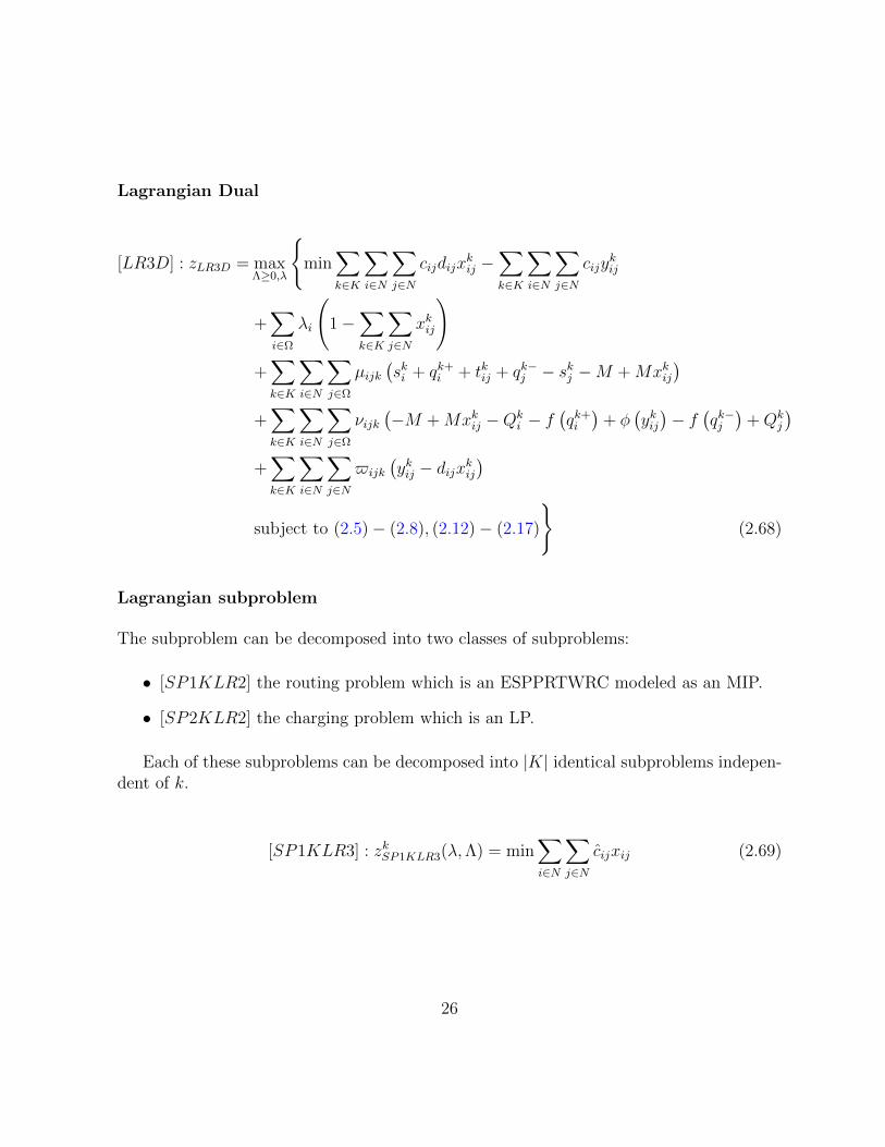
The subproblem can be decomposed into two classes of subproblems:

• [SP1KLR2] the routing problem which is an ESPPRTWRC modeled as an MIP.

• [SP2KLR2] the charging problem which is an LP.

Each of these subproblems can be decomposed into |K| identical subproblems indepen-dent of k.

[SP1KLR3] : zkSP1KLR3(λ,Λ) = min∑i∈N

∑j∈N

cijxij (2.69)

26

subject to ∑j∈N

x0j = 1 (2.70)∑i∈N

xil −∑j∈N

xlj = 0 ∀l ∈ Ω (2.71)∑i∈ω

hi∑j∈N

xij ≤ C (2.72)

ai ≤ si ≤ bi ∀i ∈ N (2.73)

si + tij − sj ≤M (1− xij) ∀i ∈ Ω,∀j ∈ N (2.74)

xij ∈ 0, 1 ∀i ∈ N (2.75)

where

c =

cijdij − λi +Mµij +Mνij −$ijdij ∀i ∈ Ω,∀j ∈ Ωcijdij − λi −$ijdij ∀i ∈ Ω, j = 0cijdij +Mµij +Mνij −$ijdij i = 0,∀j ∈ Ω

(2.76)

[SP2KLR3] : zSP2KLR3(λ,Λ) = min∑i∈N

∑j∈N

−cijyij +∑i∈N

ciq+i +

∑j∈N

cjq−j +

∑i∈N

cisi+∑i∈N

ciQi (2.77)

subject to

φ (yij) ≤ Qi + f(q+i

)∀i, j ∈ N (2.78)

yij ≤ dij ∀i, j ∈ N (2.79)

Qi + f(q+i

)≤ E ∀i ∈ N (2.80)

yij, q+i , q

−i ≥ 0 ∀i, j ∈ N (2.81)

si, Qi ≥ 0 ∀i ∈ N (2.82)

27

where

c =

cij − νijτ −$ij ∀i ∈ N,∀j ∈ Ωcij −$ij ∀i ∈ N, j = 0

(2.83)

c =∑j∈Ω

µij −∑j∈Ω

νijη ∀i ∈ N (2.84)

c =

∑i∈N µij −

∑i∈N νijη ∀j ∈ Ω

0 j = 0(2.85)

c =

∑j∈Ω µij −

∑j∈N µji ∀i ∈ Ω∑

j∈Ω µij ∀i = 0(2.86)

c =

−∑

j∈Ω µij +∑

j∈N µji ∀i ∈ Ω

−∑

j∈Ω µij ∀i = 0(2.87)

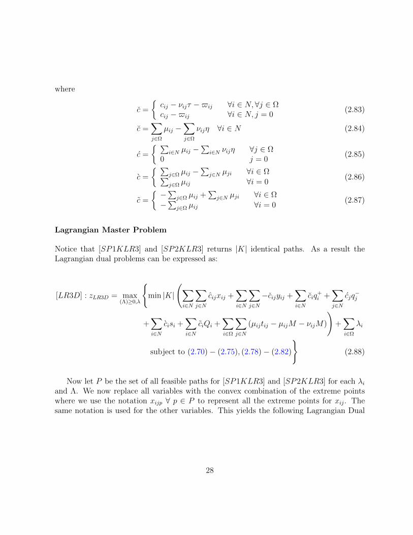
Lagrangian Master Problem

Notice that [SP1KLR3] and [SP2KLR3] returns |K| identical paths. As a result theLagrangian dual problems can be expressed as:

[LR3D] : zLR3D = max(Λ)≥0,λ

min |K|

(∑i∈N

∑j∈N

cijxij +∑i∈N

∑j∈N

−cijyij +∑i∈N

ciq+i +

∑j∈N

cjq−j

+∑i∈N

cisi +∑i∈N

ciQi +∑i∈Ω

∑j∈N

(µijtij − µijM − νijM)

)+∑i∈Ω

λi

subject to (2.70)− (2.75), (2.78)− (2.82)

(2.88)

Now let P be the set of all feasible paths for [SP1KLR3] and [SP2KLR3] for each λiand Λ. We now replace all variables with the convex combination of the extreme pointswhere we use the notation xijp ∀ p ∈ P to represent all the extreme points for xij. Thesame notation is used for the other variables. This yields the following Lagrangian Dual

28

representation:

[LR3D] : zLR3D = maxΛ≥0,λ

minP|K|

(cp −

∑i∈Ω

aipλi +∑i∈Ω

∑j∈N

M(µij + νij)xijp −∑i∈N

∑j∈N

$ijdijxijp

+∑i∈N

∑j∈Ω

νijτyijp +∑i∈N

∑j∈N

$ijyijp +∑i∈N

∑j∈Ω

(µij − νijτ )q+ip

+∑i∈N

∑j∈Ω

(µij − νijτ )q−ip +∑i∈N

∑j∈Ω

µijsip −∑i∈N

∑j∈Ω

µijsjp −∑i∈N

∑j∈Ω

µijQip

+∑i∈N

∑j∈Ω

µijQjp +∑i∈Ω

∑j∈N

(µijtij − µijM − νijM)

)+∑i∈Ω

λi (2.89)

where

cp = ckp =∑

(i,j)∈A

ckijdkijx

kij −

∑(i,j)∈A

ckijykij ∀k ∈ K, ∀p ∈ P k (2.90)

aip = akip =∑j∈N :j

xijp ∀k ∈ K, ∀i ∈ N, ∀p ∈ P k (2.91)

After rearranging the terms with respect to the dual variables we get the followingrepresentation of the Lagrangian Dual problem:

[LR3D] : zLR3D = maxΛ≥0,λ

minP|K|

(cp −

∑i∈Ω

aipλi∑i∈N

∑j∈Ω

(sip + q+

ip + tij + q−jp − sjp −M +Mxijp)µij+∑

i∈N

∑j∈Ω

(−M +Mxijp −Qip − f

(q+ip

)+ φ (yijp)− f

(q−jp)

+Qjp

)νij+

∑i∈N

∑j∈N

(yijp − dijxijp)$ij

)+∑i∈Ω

λi (2.92)

Let θ = zSP1KLR3 + zSP2KLR3

Then the master problem can be written as:

29

[LR3M ] : zLR3M = maxλ,µ,ν,$,θ

|K| θ +∑i∈N

∑j∈Ω

|K| (µijtij − µijM − νijM) +∑i∈Ω

λi (2.93)

subject to

θ ≤ cp −∑i∈Ω

aipλi

+∑i∈N

∑j∈Ω

(sip + q+

ip + q−jp − sjp +Mxijp)µij

+∑i∈N

∑j∈Ω

(Mxijp −Qip − f

(q+ip

)+ φ (yijp)− f

(q−jp)

+Qjp

)νij

+∑i∈N

∑j∈N

(yijp − dijxijp)$ij ∀p ∈ P (2.94)

θ ≤ 0 (2.95)

µij, νij, $ij ≥ 0 ∀i, j (2.96)

Lagrangian Lower Bound

For a fixed set of dual variables we obtain a Lagrangian lower bound denoted by zlag3 suchthat:

zOP ≥ zlag3(λ,Λ) = |K|

(zSP1KLR2 + zSP2KLR2 +

∑i∈N

∑j∈Ω

(µijtij − µijM − νijM)

)+∑i∈Ω

λi

2.5 Heuristics for Obtaining an Upper Bound

We use Algorithm (1) in order to find a feasible upper bound to the problem. The heuristicstarts once the best Lagrangian bound is obtained. Using the DW master problem wecollect the paths for which ω ≥ 1. If some nodes are not visited we look for the paths thatvisits only a subset of the nodes that are not visited. If still we do not obtain a feasiblepath, we solve the subproblem over a subgraph that consists only of the depot and the

30

remaining nodes which are not visited. Once done, a feasible solution is reported if thecollected paths are less than the available number of vehicles.

Require: Lagrangian bound is found1: collectedpaths← 2: visitednodes← 3: notvisitednodes← Ω4: if ω ≥ 0.9 then5: collectedpaths← collectedpaths ∪ nodesp6: visitednodes← notvisitednodes ∩ nodesp7: notvisitednodes← notvisitednodes\nodesp8: end if9: while notvisited is not empty do

10: use lagragian subproblem to generate a path over the subgraph containing notvisitednodesonly in addition to the depot

11: collectedpaths← collectedpaths ∪ nodesp12: visitednodes← notvisitednodes ∩ nodesp13: notvisitednodes← notvisitednodes\nodesp14: end while15: if |collectedpaths| ≤ |K| then16: a feasible solution in found17: end if

Algorithm 1: Heuristic to find a feasible solution

2.6 Computational Results

In this section, we report 3 sets of computational results. The first set compares the qualityof the lower bounds obtained by the three different Lagrangian relaxations. The second setcompares the quality of the lower bound obtained by Lagrangian relaxation 1 (LR1) withoptimal solution obtained by Cplex. Finally, we report the solution of the data sets whichLR1 was able to find a Lagrangian bound along with optimal solution when available.In these results, we use a subset of nodes in particular the first 16, 25, and 30 nodes ofSolomon’s instances. These results will be used later in Chapter 3 to evaluate the qualityof the tabu search solutions. The algorithms were implemented using Matlab and run on aLenovo workstation with 64-bit windows 7, 2.3 GHZ CPU processor, and 48 GB of RAM.

2.6.1 Solomon’s Instances

Solomon’s well-known instances are the classical benchmark data sets which have beenused extensively in the literature on routing problems. The instances were first proposedby Solomon [1987] based on some data sets presented by Christofides et al. [1979]. Solomon[1987] proposed a total of 56 data sets each consisting of 100 customers with their coor-dinates, a central depot, number of vehicles, capacity limits, time windows, and service

31

times. However, in the literature it is common to use a subset of the 100 customers likefirst 25 or 50 customers of the set. There is a total of 56 datasets classified into 6 classesas follows:

• R1xx consists of 12 datasets and contains customers which are located randomlyusing a random uniform distribution with short time horizons.

• R2xx consists of 11 datasets and contains customers which are located randomlyusing a random uniform distribution with long time horizons.

• C1xx consists of 9 datasets and contains customers which are clustered with shorttime horizons.

• C2xx consists of 8 datasets and contains customers which are clustered with longtime horizons.

• RC1xx consists of 8 datasets and contains a mix of clustered and randomly locatedcustomers with short time horizons.

• RC2xx consists of 8 datasets and contains a mix of clustered and randomly locatedcustomers with long time horizons.

2.6.2 PHEVRPTW additional Parameters

We use realistic values to characterize the properties of the plug-in hybrid vehicles used.We assume all vehicles have a battery with a capacity of 20 kWh, charging rate of 5kWh/hr and a charge depletion rate of 1 KWh/mi. We assume that the coordinates inSolomon’s instances are given in miles and the time in minutes. We assume the gasolinecost to be $3.5/gallon while the charging cost to be negligible. All vehicles start at thedepot on fully charged batteries and the time window for coming back to the depot to beinfinite. We set the travel time (in mins) between the nodes to be equal to the distancebetween the nodes (in mi). Finally, we ignore the service times at each node to allowfor more charging and discharging time. We also assume that there is enough number ofvehicles (K = 50). Clearly, these assumptions can be made with out loss of generality.

2.6.3 Lower Bound Comparison

We first compare the quality of the lower bounds of the Lagrangian relaxation 1 (LR1), La-grangian relaxation 2 (LR2), and Lagrangian relaxation 3 (LR3). We use the dataset R101

32

as a benchmark using small sets of customers (max 16 customers) of Solomon instances.The results are summarized in Table 2.1.

Table 2.1: Comparison of the Lagrangian bounds obtained by 3 relaxations

LR1 LR2 LR3

Iterations time (s) zlag Iterations time (s) zlag Iterations time (s) zlag

R101 4 nodes 8 0.55 3.43 14 0.55 1.77 91 3.52 0.00

R101 8 nodes 23 2.02 7.82 51 1.92 3.51 1104 153.60 0.00

R101 10 nodes 32 3.54 14.92 80 3.25 6.32 2787 1779.09 0.00

R101 16 nodes 62 19.79 40.65 57 3.22 10.62 3170 34410.00 N/A

We can observe that the LR3 performs very badly even for very small datasets. TheLagrangian bounds obtained from LR3 are the worse and of potentially no use from analgorithmic effort since it is very far away from LR1. In addition, as the the numberof customers increase the convergence of the cutting plane becomes very slow as the cutsobtained from the ESPPRCTW are very weak. As for LR2, we can see that the Lagrangianbound is better than LR3 but is still very far from LR1. Clearly, LR1 has the bestLagrangian bound but we notice that even for small data sets Cplex struggles with thesubproblem.

2.6.4 LR1 v.s. Cplex

In this section, we summarize the computational results of our algorithm implemented on6 of the famous Solomon Instances. The instances were reduced from 100 nodes and 25vehicles to 16 nodes and 5 vehicles. The algorithm was implemented using Matlab andwere solved on a Dell Latitude E6400 with 4 GB RAM running at 2.4 GHz. We summarizeour results in Table 2.2.

Despite its simplicity, the proposed heuristics to get a feasible solution provides theoptimal solution in many of the instances. Of course, more sophisticated algorithms canbe proposed which can improve this heuristics even further. In terms of the quality ofthe solution, we notice the Lagrangian bound is extremely tight as it is within 1% of theoptimal value provided by Cplex.

33

Table 2.2: Computational Results using 16 nodes of some Solomon instances

Lagrangian Relaxation Heuristic Cplex

Instances zlag time (s) SP time (s) Iterations Feasobj final time (s) Gap sol time(s) Gap

R101 16 36.786 7.416 6.956 49 36.992 7.445 1% 36.992 904.712 1%

R201 16 9.068 52.809 51.971 81 9.068 52.846 0% 9.068 4.368 0%

C101 16 2.972 9.507 8.970 65 3.259 9.908 10% 2.972 9.594 0%

C201 16 4.949 8.337 7.802 76 4.949 10.277 0% 4.949 2.512 0%

RC101 16 28.798 99.626 99.086 64 33.832 103.171 17% 29.004 3353.800 1%

RC201 16 14.069 80.024 78.606 112 14.069 80.057 0% 14.069 4.602 0%

2.6.5 LR1 Complete Results

The LR1 Lagrangian relaxation was applied to all of the Solomon’s instances (R1, R2, C1,C2, RC1, and RC2) using the first 16, 25, and 30 customers and a cutting-plane iterativeapproach. The subproblem was attacked aggressively by all possible cuts in Cplex. Inaddition, the subproblem algorithm was set to return a pool of negative reduced costsolutions (max of 20 solutions) instead of a single optimal solution only. The time limiton the subproblem was set to 600s and the overall problem to 6500s. The results aresummarized in Table 2.3.

We notice from the table, that the proposed Lagrangian relaxation is very efficient incomputing very tight lower bounds however the subproblem is very heavy and cannot besolved efficiently using Cplex. In addition, due to the continuous nature of the charge level,this subproblem cannot be solved using the known label correcting algorithms used for theclassical VRPTW.

2.7 Conclusion

As the technology of batteries advances and their cost decreases, plug-in hybrid vehicles(PHEVs) have the potential to become the ubiquitous transportation technology in supplychains due to their potential savings on gasoline costs and the flexibility provided byoperating on both internal combustion engines and electric charge. In this chapter, wepresented a novel formulation for the Plug-in-Hybrid electric vehicle routing problem withtime windows (PHEVRPTW). The problem is an extension of the classical vehicle routingproblem with time windows (VRPTW) where the vehicles used are plug-in hybrid.

Due to the different type of vehicles, the classical shortest path thinking paradigm

34

Table 2.3: LR1 Results on Solomon instances 16-30 nodesDataset Lag time (s) Heuristic time (s) Total Time (s) Zmaster Zlag OPT Gap

R101 16nodes 7.16 0.01 7.18 26.27 26.27 26.27 0%

R101 25nodes 23.93 0.17 24.10 43.62 43.62 43.75 0%

R101 30nodes 61.17 0.00 61.18 45.25 45.25 45.25 0%

R102 16nodes 5217 0.01 5217 19.97 19.97 19.97 0%

R105 16nodes 49 0.00 49 25.23 25.23 25.23 0%

R105 25nodes 1583 0.00 1583 41.16 41.16 41.16 0%

R105 30nodes 5581 0.00 5581 42.66 42.66 42.66 0%

R109 16nodes 2054 0.09 2054 23.93 23.93 24.17 1%

R201 16nodes 96 0.00 96 9.09 9.09 9.09 0%

R202 16nodes 2486 0.00 2486 4.95 4.95 4.95 0%

R203 16nodes 2349 0.00 2349 3.02 3.02 3.02 0%

R209 16nodes 5906 0.07 5907 3.78 3.78 - -

R210 16nodes 5022 0.00 5022 3.02 3.02 3.02 0%

C101 16nodes 38 0.08 39 2.97 2.97 2.97 0%

C101 25nodes 306 0.20 306 3.16 3.16 - -

C101 30nodes 1080 0.60 1081 3.16 3.16 - -

C105 16nodes 87 0.24 87 1.80 1.80 - -

C105 25nodes 2800 0.11 2801 2.54 2.54 2.54 0%

C105 30nodes 5828 0.47 5828 2.54 2.54 2.54 0%

C106 16nodes 43 0.07 43 2.97 2.97 3.02 2%

C106 25nodes 458 0.21 458 3.12 3.12 - -

C106 30nodes 1449 0.44 1450 3.12 3.12 - -

C107 16nodes 112 0.07 112 0.54 0.54 - -

C108 16nodes 79 0.07 79 0.00 0.00 0.00 0%

C109 16nodes 52 0.07 52 0.00 0.00 - -

C109 25nodes 2703 0.21 2703 0.00 0.00 - -

C201 16nodes 46 0.00 46 5.52 5.52 5.52 0%

C201 25nodes 103 0.00 103 1.17 1.17 1.17 0%

C201 30nodes 130 0.31 130 1.17 1.17 - -

C202 16nodes 106 0.00 106 3.64 3.64 3.64 0%

C202 25nodes 2473 0.05 2473 0.00 0.00 1.91 0%

C203 16nodes 435 3.05 438 3.64 3.64 - -

C204 16nodes 332 0.00 332 2.59 2.59 2.59 0%

C205 16nodes 127 0.51 128 4.49 4.49 - -

C205 25nodes 797 0.04 798 0.71 0.71 - -

C205 30nodes 4040 0.34 4040 0.71 0.70 - -

C206 16nodes 131 0.00 131 4.49 4.49 4.49 0%

C206 25nodes 4397 0.04 4397 0.71 0.70 - -

C207 16nodes 118 0.00 118 3.64 3.64 3.64 0%

C208 16nodes 180 0.00 180 3.87 3.87 3.87 0%

RC101 16nodes 505 0.07 505 29.71 29.71 - -

RC101 25nodes 4279 0.44 4280 50.08 50.07 - -

RC101 30nodes 5765 0.18 5765 69.62 69.62 - -

RC201 16nodes 66 0.00 66 14.07 14.07 14.07 0%

RC201 25nodes 3044 0.00 3044 22.26 22.09 22.26 0%

35

is not optimal anymore. Hence, the decision process is more complicated, as additionalconsideration should be given to the charging and discharging patterns of the batterywhile meeting the time windows of each customer. Since this is a new problem and has notbeen studied before, we experiment with three different Lagrangian relaxations to study thequality of lower bounds obtained. The computational results show that the best Lagrangianbound is obtained by using similar relaxation approaches to the classical VRPTW. Howeverthe resultant subproblem is different from the classical elementary shortest path problemwith resource constraints and the classical label correcting algorithms available in theliterature are not suitable for solving this subproblem.

The Lagrangian relaxation approach was implemented using the cutting plane algo-rithm. Solving the subproblem generates a valid cut to be added to the master problemwhich, in return, updates the Lagrangian parameters of the subproblem. The master prob-lem is an LP while the subproblem is an MIP which were both solved using Cplex. Wereported our results using Solomon’s instances which are classical for any routing prob-lem. The PHEVRPTW proves to be a hard problem to be solved where only a subset ofSolomon’s instances with customers ranging between 16 and 30 were solved. The maximumwe were able to solve, is only two datasets with 50 customers given the time limit (6500s).

The scope of this chapter was not to provide the most efficient algorithm for PHEVRPTW.However, it is the first step towards a novel set of problems. Any extension of the classicalPHEVRPTW can be considered a potential extension of the PHEVRPTW. Our approachwas focused on studying different possible Lagrangian relaxations and identifying researchchallenges and gaps related to this new set of problems. In the next chapter, we presenta tabu search algorithm specific to the PHEVRPTW and we report the first results onSolomon’s datasets with 100 customers.

36

Chapter 3

Tabu Search Algorithm

The traditional vehicle routing problem with time windows has been studied intensivelyusing both exact and heuristics algorithm. While Lagrangian relaxation and column gen-eration are the common approaches for exact algorithms, there is a wide range of differentproposed heuristics in the literature. Over the past years, meta-heuristics have been suc-cessfully used to provide optimal or near optimal solutions to a wide range of combinatorialoptimization problems. Some of the most successful and widely used meta-heuristics are:simulated annealing [Kirkpatrick et al., 1983], [Aarts and Korst, 1988], [van Laarhovenand Aarts, 1987], genetic algorithms [Holland and Reitman, 1977], [Goldberg and Holland,1988], [Davis, 1991], [Dorigo and Stutzle, 2010], particle swarm [Kennedy and Eberhart,1995], [Clerc, 2006], memetic algorithms [Moscato, 1989], [Moscato and Cotta, 2003], andtabu search [Glover, 1989], [Glover, 1990], [Glover and Laguna, 1998].

In this chapter, we focus on tabu search algorithms due to their renowned success forvehicle routing problems. In fact, one can argue that the reputation of the tabu searchalgorithms is due to their widespread success in providing high quality solutions for differentvariants of routing problems. Tabu search is considered a local search meta-heuristic wherea local neighborhood of a current solution is evaluated based on a devised cost evaluationfunction to decide on the next solution. Most tabu search algorithms use an elitist strategyto choose the next best solution however some attempt to diversify their choices. One ofthe most distinctive features of the tabu search algorithms is the tabu list which preventscycling. The tabu list helps to escape local optimal solutions. The basic idea is to keep alist of attributes of previous moves in the form of a tabu list to restrict these moves untila certain number of iterations have passed. Some exceptions exist for cases when theserestricted moves can improve the best incumbent solution. This approach has been first

37

formalized by Cordeau et al. [1997] and is commonly referred to as the aspiration criteria.This search process is continued until a certain stopping criteria is reached.

3.1 Literature Review

The literature on heuristics and their different applications is vast however we will focuson the literature related to vehicle routing problems. Most of the heuristics proposed forthe vehicle routing problems with time windows have first been successfully applied tothe traveling salesman problem (TSP) and the traditional vehicle routing problem (VRP)and have been later adapted to account for time windows requirements by using a simplefeasibility check or applying a large penalty for violating the time windows restrictions.

The earliest forms of heuristics for routing problems are generally referred to as classicalheuristics as denoted by Laporte and Semet [2002] and Cordeau et al. [2006]. These classicalheuristics algorithms can be further classified as: (1) construction heuristics, (2) two-phaseheuristics, and (3) route improvement heuristics.

The most famous construction heuristic is the savings algorithm proposed by Clarke andWright [1964] for the VRP. The algorithm merges two separate routes into a single feasibleroute if a certain savings criteria is satisfied. In particular two routes r1 = 0, · · · , ni, 0and r2 = 0, nj, · · · , 0 are merged to a single route r′12 = 0, · · · , ni, nj, · · · , 0 if sij =c(ni, 0) + c(0, nj) − c(i, j). Several other variants for the savings algorithm with addi-tional savings weights and different merging processes have been proposed, for examplesee [Gaskell, 1967], [Yellow, 1970], [Golden et al., 1977], [Paessens, 1988], [Nelson et al.,1985]... It is worth mentioning that the first attempt to adapt the savings algorithm forthe VRPTW was made by Solomon [1987] by accounting for the route orientations in themerging process and time feasibility. However, the results were not promising as the av-erage deviation from the best known solution for R1 sets and C1 sets was 22% and 17%compared to an average of 0% on both data sets for another insertion heuristic denoted byI1 which we will discuss later.

The two-phase heuristics, also known as “cluster-first route-second” splits the routingproblem into two well known optimization problems. The first is partitioning the customersinto separate clusters where each cluster represents a separate route served by a separatevehicle. This is normally modeled as a generalized assignment problem. The second is aTSP problem to determine the scheduling of the customers in each cluster. One of themost famous algorithms which belongs to this category is the sweep algorithm which waspopularized by Gillett and Miller [1974] but was first introduced by Wren and Holliday

38

[1972]. The idea is to cluster the products based on their polar coordinates with respect tothe depot. Gillett and Miller [1974] described two versions of the algorithm called forwardand backward sweep algorithms. In the forward algorithm, the customers are sorted basedon the smallest polar coordinates first. Next, customers are inserted sequentially to theseeded route until the capacity is full where a new route is seeded by the next customer inthe list. In the backward sweep algorithm, the customers are sorted based on the largestpolar coordinates first. Further, intra-routes improvements were also described in theirpaper. Different variants of the two-phase heuristics have been proposed by Foster andRyan [1976], Ryan et al. [1993], Fisher and Jaikumar [1981], and Bramel and Simchi-Levi[1995]. Solomon [1987] also presented an extension of the sweep algorithm for the VRPTW.The proposed algorithm was superior to the savings algorithm yet it was dominated by theI1 insertion heuristic.

The push forward (PF) heuristic was first described in Solomon [1987] as a sequen-tial method to account for the adjustments needed to the service time of the subsequentcustomers due to the insertion of a new customer. In addition, Solomon [1987] proposedseveral extensions for the savings and sweep heuristics to account for the temporal aspectof the problem. Most importantly, Solomon proposed 3 different insertion heuristics; I1

which accounts for the savings as a weighted sum of the distance and the unnecessarywaiting due to hard time windows; I2 which accounts for the savings as a weighted sum ofthe distance and total traveling time; I3 is similar to I1 but the width of the time windowof the newly inserted customer is added to the weighted average savings. In terms of totaltransportation costs, I1 insertions outperformed the other heuristics. In addition to theinsertion heuristic, Solomon [1987] described two initialization procedures to start a routeseed, (a) use the farthest unrouted customers and (b) use the unrouted customer with theearliest deadline. Later, Thangiah et al. [1994] coined the term push forward insertionheuristic (PFIH) to represent Solomon’s PF mechanism along with Solomon’s I1 insertionheuristic. However, for initializing the route seed they also add a weight to the clusteringapproach similar to that proposed in the sweep algorithm. A detailed description of thePFIH is presented in section 3.2.2.

In addition to these construction heuristics, several authors proposed several routeimprovement heuristics which are implemented on top of the construction heuristics. Theseimprovement heuristics can be classified into two categories (1) intra-route heuristics and(2) inter-route heuristics. As the name suggests, intra-route heuristics are heuristics focuson the improvement of individual routes separately by various operations like swapping,removing, and adding customers to a single route. Most intra-route heuristics have beenfirst developed to solve the TSP problem since by definition the TSP is a single Hamiltoniancycle/route. The most famous intra-route heuristics are the k-opt exchanges Lin [1965]

39

and Or-opt by Or [1976]. On the other hand, inter-route heuristics focus on improvementsacross several routes mainly through interchange heuristics. The most famous inter-routeheuristics are the ejection chains Glover [1992], k-opt∗ Potvin and Rousseau [1995], theλ-interchange by Osman [1993], and CROSS-exchange Taillard et al. [1997]. These routesimprovements provide the basis of the neighborhood generation mechanism in the besttabu search algorithms in the literature for different routing problem variants.

Another track of heuristics used in combinatorial optimization is “meta-heuristics”.Meta-heuristics has been defined by Osman and Laporte [1996] as:

“... a class of approximate method ... designed to attack complex optimiza-tion problems where classical heuristics and optimization methods have failedto be effective and efficient. A meta-heuristic is formally defined as an it-erative generation process which guides a subordinate heuristic by combiningintelligently different concepts for exploring and exploiting the search space,learning strategies are used to structure information in order to find efficientlynear-optimal solutions.”

Although it is hard to characterize these meta-heuristics into well structured categories, itis common to classify meta-heuristic algorithms by two search strategies (1) local searchand (2) population search.

Most local search algorithms move sequentially from one solution to another in anapproach similar to decent algorithms while implementing different strategies to escapelocally optimal solutions. The most famous local search meta-heuristics include: tabusearch (TS) [Glover, 1986], simulated annealing (SA) [Kirkpatrick et al., 1983], and variableneighborhood search (VNS) [Mladenovic and Hansen, 1997].

On the other hand, population based heuristics commonly iterate between differentpopulation of solutions. The most common strategies are classified as evolutionary al-gorithms such as genetic algorithms (GA) [Goldberg and Holland, 1988], and learningalgorithms known as swarm intelligence (SI) such as ant colony optimization (ACO) andparticle swarm optimization (PSO). Several hybrid algorithms have been proposed in lit-erature which integrates both local and population search strategies and several differentheuristics combined [Thangiah, 1998]. A very well known example is memetic algorithmsproposed by Moscato [1989]. It is noted that Nagata et al. [2010] has recently proposed avery efficient memetic algorithm which was able to improve 184 best-known solutions outof the 356 available instances in the literature.

Out of all these meta-heuristics, tabu search algorithms have been well known fortheir success in vehicle routing problems and this explains the abundance of tabu search

40

algorithms proposed for various vehicle routing problems [Cordeau and Laporte, 2005]. Wewill limit ourselves to discussing the literature of tabu search, however readers interestedin other meta-heuristics are referred to [Gendreau and Potvin, 2010].

Tabu search was first introduced by Glover [1986] based on ideas developed in [Glover,1977]. The first implementation to solve the classical VRP is attributed to Willard [1989]who used a simple k-opt neighborhood generation mechanism. They merged the multipleroutes into a single TSP route by replicating the depot as a connecting node. Later,Osman [1993] proposed a new neighborhood generation mechanism called λ-interchangeto solve the classical VRP problem. The λ-interchange allows for up to λ nodes to beexchanged between a pair of routes. Taillard [1993] presented a parallelized tabu searchbased on λ-interchange. They defined a cost evaluation function which allows for furtherdiversification of the solution pool by adding a penalty cost for the frequency of the moveleading to this solution. They also did a periodic optimization of the the routes using anexact TSP algorithm. Another successful implementation for tabu search is the Tabourouteby Gendreau et al. [1994] which uses the GENIUS insertion heuristic proposed for TSP byGendreau et al. [1992]. This algorithm integrates a generalized insertion heuristic (GENI)and a post optimization mechanism based on unstringing and stringing (US) of nodes.Another interesting implementation for tabu search is the adaptive memory procedure(AMP) which was proposed by Rochat and Taillard [1995]. They were able to demonstratethe benefits of diversification and intensification strategies. The AMP keeps track of thebest solutions during a tabu search run, then uses a probabilistic approach to select one ofthese solutions to restart the tabu search as an initial solution. Taillard et al. [1997] adaptedthis approach to solve the VRP with soft time windows. Similar diversification strategieshave been implemented successfully by Chiang and Russell [1997] and Schulze and Fahle[1999]. Other strategies for tabu search are based on the ejection chains neighborhooddefinitions have been implemented by Xu and Kelly [1996], Rego and Roucairol [1996],and Rego [1998].

3.2 Algorithm Description

In this section, we present a Tabu search algorithm to solve the plug-in hybrid electricvehicle routing problem with time windows (PHEVRPTW).

41

3.2.1 Overall Framework for the Tabu Search

The tabu search algorithm integrates all the previous heuristics to search for a near optimalsolution in a systemic way while implementing a tabu list to avoid cycling. The algorithm isinitiated using the push forward insertion heuristic with an LP post optimization algorithmto decide on the charging and discharging patterns. A neighborhood is generated basedon a 2-interchange mechanism where only the best solution of all possible interchanges foreach pair of routes is kept in the neighborhood of the solution. The algorithm exploresthe neighborhood to find the best non-tabu move. Then an acceptance criteria based onaspiration criteria and a simulated annealing procedure is used to the next move. Thesolution quality is estimated based on the cost insertion function 3.2. The algorithm isstopped once the best solution does not improve for 10 consecutive iterations. The general

42

framework for the implemented tabu search is summarized in Algorithm 2.

Require: Feasible Problem Set1: TabuList← φ2: IncumbentSolution←∞3: k ← numberofvehicles4: C ← Capacity5: S ← PFIH6: S ← 2opt(PFIH)7: S ← half(S)8: while Not Stopping Criteria do9: Generate Neighborhood Nλ(S)

10: S ′ ←MinCost(Nλ(S))11: if S ′ ∈ TabuList then12: if Cost(S ′) < IncumberSolution then13: S ← S ′

14: end if15: else16: if Cost(S ′) < Cost(S) then17: S ← S ′

18: TabuList← TabuList ∪Move19: end if20: else21: Simulated Annealing Criteria22: end if23: end while

Require: Stopping Criteria24: BestSolution← LPoptimized(Incumbent)25: Restart using BestSolution

Algorithm 2: Tabu Search Framework

3.2.2 Initialization

In order to initialize the tabu search algorithm we use the well know push forward insertionheuristic (PFIH) which was first introduced by Solomon [1987]. The PFIH gives priorityto route customers which are farthest away from the depot. These are normally harder toassign to a route in a later stage due to the time and capacity restrictions. The customers

43

are sorted in ascending order according to the following function:

Cj = −αd0j + βbj + γ(θjd0j

360) (3.1)

where θj is the polar coordinate angle between customer j and the depot.

The unrouted customer with the lowest value is first assigned to a route. This isrepeated for every unrouted customer every time a new route needs to be constructed.This classification tends to favor the customers that are farthest from the depot and whohas the earliest time window deadline. After experimentation, the values of (α, β, γ) arechosen to be (1, 0.1, 0.7).

After the first customer is assigned, the PFIH then iteratively chooses the unroutedcustomer with the cheapest feasible insertion cost and adds it to the route. This is repeateduntil either all customers are routed or the capacity of the vehicle is exceeded or non ofthe possible insertions is feasible. If there are still unrouted customers, a new route isstarted based on 3.1 and the cheapest insertion is continued. The PFIH does not have anyrestriction on the number of vehicles available but since its priority is to fill the vehicles upto the maximum possible capacity, then the algorithm normally uses the minimum possible

44

number of vehicles. The algorithm for PFIH is summarized in Algorithm 3.

1: collectedroutes← 2: currentpath← 3: unroutedcustomers← Ω4: while unroutedcustomers is not empty do5: Start a new path6: Sort unroutedcustomers based on 3.17: Pick first sortedcustomer8: while collecteddemand+ demand(sortedcustomer(1)) <= vehiclecapacity do9: find cheapest insertion location

10: if istimefeasible then11: currentpath← currentpath ∪ sortedcustomer(1) at the cheapest location

index12: collecteddemand← collecteddemand+ demand (sortedcustomer(1))13: unroutedcustomers← unroutedcustomers\ sortedcustomer(1)14: end if15: Pick first sortedcustomer16: end while17: collectedroutes← collectedroutes ∪ currentpath18: end while19: if |collectedroutes| ≤ |K| then20: a feasible solution in found21: LP optimize the charges on the given fixed routes22: Bestroutes← postLProute23: end if

Algorithm 3: Push First Insertion Heuristic

However, to intensify the diversification we break down the routes by half to increasethe number of possible routes. We use a crossover operator to split each route at themidpoint to two separate routes. The rational behind this approach is that the designof the λ-interchange allows closing certain routes however it does not allow opening newroutes when needed. For this reason, breaking down the routes by half, allows for a largerdiversification of the solution space. Our experience with this approach is that it has beenvery effective in improving the solution quality.

45

3.2.3 Neighborhood Generation

The tabu search algorithm is a local search algorithm which success depends on the defini-tion of the neighborhood and the efficient evaluation of the best moves in this neighborhood.There has been a number of successful neighborhood generation mechanisms of which wenote:

• k-opt exchanges by Lin [1965] which was first used to generate solutions for the trav-eling salesman problem. The k-opt exchanges is an intra-route approach which allowsfor k edges to be removed from a route and replaced by k new edges while preservingthe feasibility of the route. However, this procedure is not well suited for routingproblems with time windows since it does not preserve the orientation of the routes.

• OR-opt∗ is an intra-route operator which was first introduced by Or [1976] also forthe traveling salesman problem. The idea is to relocate a chain of consecutive nodesfrom one position to another while preserving the orientation of the route.

• k-opt∗ exchange is an inter-route operator which was first introduced by Potvin andRousseau [1995]. This approach adapts the k-opt exchanges to routing problems withtime windows by preserving the orientation of the routes. The basic idea is similarto a single crossover approach implemented in genetic algorithm. Two routes areimproved by removing edge (i, i + 1) from the first route and (k, k + 1) from thesecond route and then connecting (i, k + 1) and (k, i+ 1).

• CROSS-exchange is another inter-route operator which was first introduced by Tail-lard et al. [1997]. As its name suggests, it is a generalization of the 2-opt∗ exchangewhere it resembles a 2-point cross-over in the genetic algorithm context. The idea isto remove two edges (i− 1, i) and (j, j+ 1) from the first route and (l− 1, l) and (k,k + 1) from the second route. Then the whole link i− j is exchanged with link l− kby connecting edges (i − 1, l) and (j, k + 1) for the updated first route and edges(l − 1, i) and (k, j + 1) for the updated second route.

Other commonly used neighborhood search mechanisms involve ejection chains by Glover[1992] and GENI-exchange by Gendreau et al. [1992]

46

λ - Interchange

In our tabu search algorithm, we adopt the λ- interchange mechanism which has been firstproposed by Osman [1993]. The idea is to interchange up to λ consecutive nodes betweentwo distinct routes. The most commonly used λ values is either 1 or 2. For λ=2 the set ofpossible moves are

• (0, 1): remove one node from the second route and add it to the first route.

• (0, 2): remove two nodes from the second route and add them to the first route.

• (1, 0): remove one node from the first route and add it to the second route.

• (2, 0): remove two nodes from the first route and them to the second route.

• (1, 2): interchange two nodes from second route with one node from the first route.

• (2, 1): interchange two nodes from the first route with one node from the secondroute.

• (2, 2): interchange two nodes from the first route with two nodes from the secondroute.

For each possible λ-combination (for example (1, 2)) the interchanges are investigatedat each possible position in the routes. Hence each combination produces one alternativepair of routes. The new set of routes which involves the newly modified routes is consideredas a single possible neighbor of the current solution. To generate the full neighborhood,each possible λ combination is investigated and each possible pair or routes undergo theseλ-interchanges. The set of routes are defined as an array of routes from and to the depotdenoting the sequence of nodes visited.

3.2.4 Cost Evaluation Function

The tabu search is guided by a cost evaluation function to compare the solution qualityof the neighborhood. In this section, we present a new cost evaluation function which isspecific to the PHEVRPTW. We borrow from Gendreau et al. [1994] the idea of adding apenalty cost in the objective function for violating the capacity constraints and the timewindows constraint. However, Gendreau et al. [1994] uses the penalty function along withthe traditional routing cost function

∑ij cijdij which is not suitable for the PHEVRP due to

47

the potential savings of routing on a charge. Before discussing the cost evaluation functionlet us define some additional terminology. let Sl := ∪mi=1Ri : m < k be a solution withm distinct routes such that Ri := 0, ni1 , ni2 , · · · , 0 and Ri ∩Rj 6=i = φ ∀Ri, Rj ⊂ Sl. Wedenote by (nl, nk) ∈ Ri as two consecutive customers on the route Ri.

The cost evaluation function is defined as follows:

C(Rl) = C(Rl) + ρ1

∑(i,j)∈Rl

[hi − C]+ + ρ2

∑(i,j)∈Rl

[si + q+

i + tij + q−j − skj]+

(3.2)

Where C(Rl) is calculated using a dynamic program which approximates the optimalcost of a route Rl. We note that in the traditional VRPTW, C(Rl) can be computedeasily as it is simply the sum of the arc costs on a specific route. However, in the caseof the PHEVRPTW this task is more complicated as one needs to account for the con-tinuous variables related to the charging and discharging decisions and the resulting sav-ings. One way of doing that is to calculate the costs on the arcs using the traditionalway and then fix the the integer decision variables and solve an LP problem to decideon the optimal charging and discharging patterns. However, this approach is time con-suming due to the time required to generate the constraints and call Cplex to solve theresulting LP problem for each possible interchange of each pair of routes in each neigh-borhood which proves to be very inefficient. For this reason, we approximate this costusing equation 3.2 and algorithm 4. For each pair of routes in a given solution, we returnneighborhood solution with the lowest possible cost for every possible lambda. However,only the returned solution is then optimized using an LP program. Our experience withthe dynamic program is that in most of the cases it is equal to the returned LP optimalvalue yet in some cases it mildly underestimates the savings from routing on a charge.

48

Require: Feasible Solution1: previousDepartCharge(depot)← E2: accumCharge← 03: elapsedT ime← 04: totalDistanceCost← 05: totalChargeSavings← 06: for all (ni, ni+1) ∈ R(l) do7: arrivalCharge(ni)←

max(0, previousdepartCharge(ni)− distance(ni, ni+1)/dischargerate)8: preCharge(ni)← min(E − arrivalCharge(ni), availChargeT ime(ni))9: chargeAccum(ni)← arrivalCharge(ni) + preCharge(ni)

10: elapsedT ime← elapsedT ime+ travelT ime(ni, ni+1)11: totalDistanceCost← totalDistanceCost+ distanceCost(ni, ni+1)12: distanceOnCharge← previousDepartCharge(ni)− arrivalCharge(ni, ni+1)13: chargeSavings← chargeSavings− distanceOnCharge14: if earliestDueT ime(ni+1) > elapsedT ime then15: availWaitT ime(ni+1)← earliestDueT ime(ni+1)− elapsedT ime16: postCharge(ni)←

min(E − chargeAccum(ni), availWaitT ime(ni+1) ∗ chargingRate)17: elapsedT ime← earliestDueT ime(ni+1)18: else19: availWaitT ime(ni+1)← 020: postCharge(ni)← 021: end if22: previousDepartCharge(ni)← chargeAccum(ni) + postCharge(ni)23: availWaitT ime(ni+1)← availWaitT ime(ni+1)− postCharge(ni)24: end for

Algorithm 4: Dynamic program to calculate C(Rl)

If an interchange operator is applied to pairs Rl and Rk to generate a new routes Rl′

and Rk′ then the cost difference is defined according to the following function:

∆ = C(Rl) + C(Rk)− C(Rl′)− C(Rk′) (3.3)

Hence, one solution in the neighborhood is generated by choosing the new routes leadingto the minimum ∆ generated by all the possible interchanges on the given pair. The overallneighborhood is defined as the set of minimum cost possible interchanges for each possiblepair of routes and is denoted by N(S).

49

3.2.5 The Tabu List and Aspiration Criteria

The tabu search uses a short term memory of prohibited moves denoted by a tabu list.The tabu list prevents potential cycling between solutions hence allowing the algorithm toescape any potential local optima. Using the tabu list, implies that a move represented bymoving customer i from route l to route k at iteration t is not allowed until iteration t+ θwhere θ is the size of the tabu list. In our algorithm, θ was set to 15.

The aspiration criteria is very important in the VRP since re-insertion of the customeri can lead to a better solution due to the update in the solution routes even before θiterations have passed. For this reason, the aspiration criteria is used in particular casesto allow for tabu moves granted that they lead to a better incumbent solution.

3.2.6 Diversification Strategy

In order to diversify the search and prevent the homogeneity of the neighborhoods, adiversification strategy is required to force the tabu search to explore new solutions that arenot discovered yet. Most tabu search algorithms diversify the search space by penalizingrecurrent routes using a long term memory[Cordeau and Laporte, 2005]. This idea oftracking the frequency of the routes has been first proposed by Glover [1989]. However, inour proposed algorithm we adopt the idea of incorporating a hybrid simulated annealinginto the tabu search proposed by Thangiah [1999] to accept moves which are not the fittestand hence avoid being trapped in local optimality. This approach helps to diversify thesearch area by giving a higher probability for solutions with lower costs while avoidingmyopic elitism.

Simulated annealing is a one of the simplest meta-heuristics strategy which was firstproposed to solve optimization problems by Kirkpatrick et al. [1983]. Simulated Anneal-ing (SA) uses a stochastic approach to direct the search and provides better structuredrandomization procedure for diversification. The idea is very simple; when the best movedoes not lead to a better incumbent solution or any improvement over the current solution(∆ > 0) then a solution is accepted with probability e(−∆

T), where T is a parameter called

the temperature. We start with T = 20 which decreases using a cooling factor (0.01). The

50

simulated annealing diversification heuristic is summarized in Algorithm 5.

Require: ∆ > 01: T ←MaxTemperature2: while T > 0 do3: if e(−∆

T) > rand(0, 1) then

4: Accept new solution5: T ← T

(1+CoolingFactor∗T )

6: if CurrentSolution < IncumbentSolution then7: BestTemperature← T8: end if9: else

10: ResetTemperature←Max(BestTemperature, ResetTemperature2

)11: T ← ResetTemperature12: end if13: end while

Algorithm 5: Simulated Annealing Heuristic

In addition to the simulated annealing, we use a long term memory to keep track of thebest solution. We restart the solution once using this best found solution after breakingdown the routes into half.

3.3 Computational Results

In this section we present the computational results of the proposed tabu search algo-rithm for the well known Solomon’s instances (R1, R2, C1, C2, RC1, and RC2). ThePHEVRPTW is a novel problem so there is no available implementations to compare ourtabu search with. For this reason, we compare the tabu search to the Lagrangian lowerbounds presented in Chapter 2. All of these instances are subsets of Solomon’s instanceswhich include 100 customers. However, due to the complexity of the problem, the proposedLagrangian relaxation was able to provide optimal bounds for subsets of 16, 20, and 30nodes in addition to the depot (Some exceptions exist particularly for R101). We first showthe results of the tabu search on these instances in order to evaluate the solution qualityof the proposed tabu search algorithm. We then present the tabu search results for all ofthe Solomon’s instances with 100 customers.

The instances were solved on a Lenovo workstation with 64-bit windows 7, 2.3 GHZCPU processor, and 48 GB of RAM.

51

3.3.1 Comparison Tabu vs. Lagrangian Relaxation

The tabu search, just like all other heuristics algorithms, is myopic in terms of optimality.It provides no guarantee for reaching optimal solution nor an optimality gap to assess thequality of the solutions. For this reason, we first compare the solutions obtained from ourproposed tabu search algorithms to the Lagrangian lower bounds presented in Chapter 2.The comparison is summarized in Table 3.1

The gap in Table 3.1 corresponds to the gap between the tabu search solution (ztabu) andthe Lagrangian lower bound (zlag). The column titled “Vehicles” represents the numberof vehicles used in the best tabu search solution. The proposed tabu search proves to bevery effective as it was able to find solutions within less than 5% gap from the Lagrangianlower bound for 23 out of the 45 datasets. The average gap on the given data sets is 16%and the maximum resultant gap is 70%. However, the large gaps are realized only for datasets with small objective values for which any slight deviation from the optimal solutioncorresponds to a large gap.

3.3.2 Tabu Search Results for the 100 Customers Datasets

In this part, we present the tabu search result for the full datasets by Solomon with 100customers. These are the first results in the literature so it is not possible to assess thequality of these solutions. However, given the promising results on the smaller datasetswe expect the results on these larger datasets to be equally competitive at least for someinstances. These results can be used as a benchmark for future research on either exact orheuristics algorithms. The results are summarized in Tables 3.2-3.7 classified according toSolomon’s datasets types.

3.4 Conclusion

Heuristics have played an important role in the advancement of the research on vehiclerouting problems and their extensions. While the exact algorithms continue to evolveand stretch our ability to find optimal solutions efficiently, heuristics are extending ourcapability to solve larger datasets even farther. The problem with heuristics however isthat they are myopic in terms of the quality of the solutions obtained. A common approachin heuristics is to compare the results to the best known exact algorithms in order evaluatethe quality of the solutions generated by these heuristics.

52

Table 3.1: Comparison between the Lagrangian relaxation bound and the tabu searchLag Relaxation Tabu Search

Dataset Time (s) zlag Iter Time (s) Vehicles ztabu Gap

R101 16nodes 7.33 26.27 23 31.7 10 26.27 0%

R101 25nodes 30.27 43.62 54 105.9 13 44.03 1%

R101 30nodes 102.10 45.25 64 159.4 14 45.25 0%

R102 16nodes 5216.76 19.97 24 29.6 9 23.29 17%

R105 16nodes 49.17 25.23 21 27.9 10 25.23 0%

R105 25nodes 1582.79 41.16 54 89.2 15 41.43 1%

R105 30nodes 5580.73 42.66 64 150.7 15 43.07 1%

R109 16nodes 2054.39 23.93 36 26 10 24.22 1%

R201 16nodes 96.28 9.09 36 21.4 5 9.09 0%

R202 16nodes 2486.10 4.95 36 23.3 6 6.36 28%

R203 16nodes 2349.17 3.02 36 21.4 6 4.88 62%

R209 16nodes 5906.51 3.78 31 17.1 4 6.41 70%

R210 16nodes 5022.33 3.02 36 23.4 6 4.88 62%

C101 16nodes 38.52 2.97 36 25.2 8 2.97 0%

C101 25nodes 306.08 3.16 54 56.1 6 3.49 10%

C101 30nodes 1080.64 3.16 64 104.6 11 4.16 32%

C105 16nodes 86.94 1.80 36 25.1 8 2.02 12%

C105 25nodes 2800.53 2.54 54 71 9 3.21 26%

C105 30nodes 5828.48 2.54 64 113.3 14 2.54 0%

C106 16nodes 42.86 2.97 36 22.5 8 2.97 0%

C106 25nodes 458.34 3.12 54 64.4 9 3.42 10%

C106 30nodes 1449.69 3.12 64 115.1 10 3.46 11%

C107 16nodes 111.82 0.54 36 22.1 6 0.54 0%

C108 16nodes 78.98 0.00 41 24.4 6 1.46 N/A

C109 16nodes 52.08 0.00 36 16.5 4 0 0%

C109 25nodes 2703.10 0.00 44 46.5 9 2.36 N/A

C201 16nodes 45.93 5.52 36 13.5 4 5.52 0%

C201 25nodes 103.30 1.17 47 42.2 5 1.17 0%

C201 30nodes 129.99 1.17 52 64.8 5 1.17 0%

C202 16nodes 106.27 3.64 25 12.1 5 4.67 28%

C202 25nodes 2472.99 0.00 50 43.6 3 0 0%

C203 16nodes 437.89 3.64 31 14 4 4.16 14%

C204 16nodes 332.29 2.59 29 11.6 3 2.59 0%

C205 16nodes 127.66 4.49 35 12.8 4 4.49 0%

C205 25nodes 797.52 0.71 54 46.9 4 1.17 65%

C205 30nodes 4040.03 0.70 43 49.3 5 1.17 67%

C206 16nodes 130.61 4.49 36 13.3 3 4.49 0%

C206 25nodes 4397.20 0.70 39 31 4 1.07 53%

C207 16nodes 117.56 3.64 36 14 3 4.95 36%

C208 16nodes 179.72 3.87 34 13.5 3 4.95 28%

RC101 16nodes 504.59 29.71 29 14.5 4 32.13 8%

RC101 25nodes 4279.89 50.07 71 61 5 52.04 4%

RC101 30nodes 5764.78 69.62 51 63.3 6 72.19 4%

RC201 16nodes 66.18 14.07 36 15.3 3 19.67 40%

RC201 25nodes 3043.98 22.09 54 44.3 3 22.26 1%

53

Table 3.2: Tabu search results for R1xx datasets with 100 nodes

Dataset Iter Time (s) Distance Cost Charge Savings ztabu Vehicles

R101 100nodes 150 11899.8 472.8 -351.7 121.1 34

R102 100nodes 130 8823.8 476.8 -364.7 112.2 38

R103 100nodes 137 6610.3 451.4 -353.1 98.2 38

R104 100nodes 106 8691.2 412.8 -320.7 92.1 31

R105 100nodes 111 19086.8 451.1 -340.7 110.3 36

R106 100nodes 117 6308.9 462.7 -358.7 103.9 36

R107 100nodes 125 10100.2 400.9 -304.9 96.0 31

R108 100nodes 117 13182.3 382.1 -290.3 91.8 31

R109 100nodes 106 18330.9 427.5 -322.6 104.9 33

R110 100nodes 130 25577.8 386.5 -290.8 95.7 30

R111 100nodes 101 23034.9 394.1 -298.6 95.6 31

R112 100nodes 113 3145.8 354.4 -261.4 93.0 28

Table 3.3: Tabu search results for R2xx datasets with 100 nodes

Dataset Iter Time (s) Distance cost Charge Savings ztabu Vehicles

R201 100nodes 127 5436.4 369.4 -353.2 16.3 19

R202 100nodes 111 7832.9 396.8 -380.7 16.1 22

R203 100nodes 107 8420.7 353.6 -336.8 16.8 19

R204 100nodes 148 11714.6 342.3 -335.2 7.2 19

R205 100nodes 141 2845.1 367.7 -356.5 11.2 22

R206 100nodes 137 2929.4 319.6 -304.9 14.7 17

R207 100nodes 104 2912.3 329.8 -310.5 19.3 18

R208 100nodes 106 3247.5 284.4 -277.9 6.4 14

R209 100nodes 126 5720 333.9 -326.1 7.8 19

R210 100nodes 165 12771.5 358.1 -345.6 12.5 21

R211 100nodes 84 3865.2 258.2 -242.4 15.9 12

54

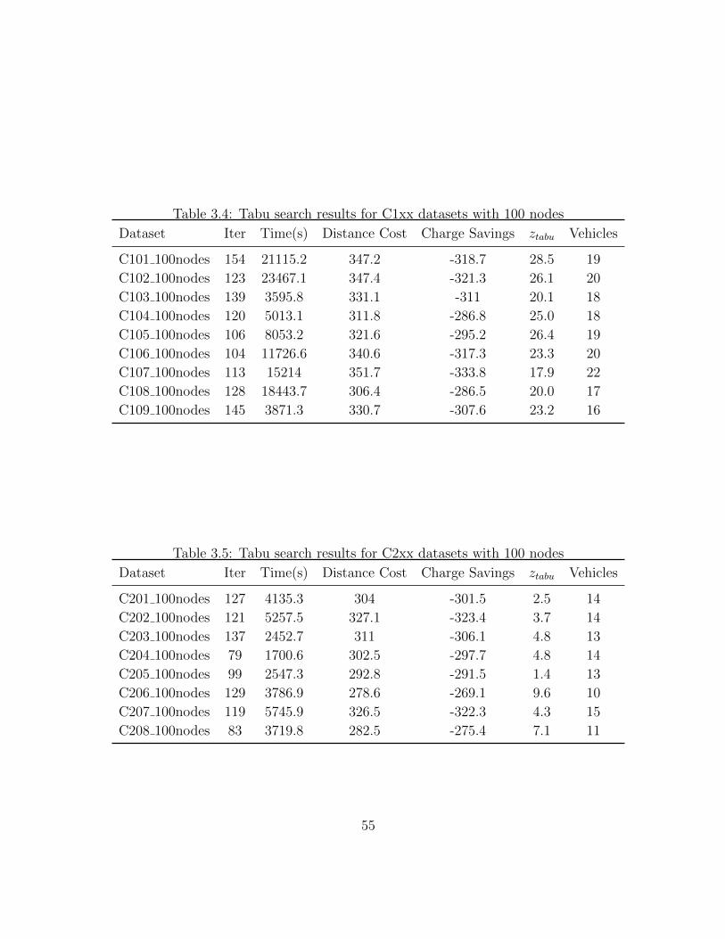
Table 3.4: Tabu search results for C1xx datasets with 100 nodes

Dataset Iter Time(s) Distance Cost Charge Savings ztabu Vehicles

C101 100nodes 154 21115.2 347.2 -318.7 28.5 19

C102 100nodes 123 23467.1 347.4 -321.3 26.1 20

C103 100nodes 139 3595.8 331.1 -311 20.1 18

C104 100nodes 120 5013.1 311.8 -286.8 25.0 18

C105 100nodes 106 8053.2 321.6 -295.2 26.4 19

C106 100nodes 104 11726.6 340.6 -317.3 23.3 20

C107 100nodes 113 15214 351.7 -333.8 17.9 22

C108 100nodes 128 18443.7 306.4 -286.5 20.0 17

C109 100nodes 145 3871.3 330.7 -307.6 23.2 16

Table 3.5: Tabu search results for C2xx datasets with 100 nodes

Dataset Iter Time(s) Distance Cost Charge Savings ztabu Vehicles

C201 100nodes 127 4135.3 304 -301.5 2.5 14

C202 100nodes 121 5257.5 327.1 -323.4 3.7 14

C203 100nodes 137 2452.7 311 -306.1 4.8 13

C204 100nodes 79 1700.6 302.5 -297.7 4.8 14

C205 100nodes 99 2547.3 292.8 -291.5 1.4 13

C206 100nodes 129 3786.9 278.6 -269.1 9.6 10

C207 100nodes 119 5745.9 326.5 -322.3 4.3 15

C208 100nodes 83 3719.8 282.5 -275.4 7.1 11

55

Table 3.6: Tabu search results for RC1xx datasets with 100 nodes

Dataset Iter Time (s) Distance Cost Charge Savings ztabu Vehicles

RC101 100nodes 115 5733.3 497.3 -317.4 179.9 33

RC102 100nodes 144 11761.6 411.7 -250.4 161.3 26

RC103 100nodes 129 19304.3 411 -270.6 140.4 29

RC104 100nodes 111 3387.7 389.1 -263.1 126.0 29

RC105 100nodes 103 5049.6 472.8 -316 156.9 33

RC106 100nodes 108 6373.8 368 -218.4 149.7 21

RC107 100nodes 114 11172.5 352.2 -223.9 128.3 21

RC108 100nodes 118 8370.4 356.3 -237.2 119.1 26

Table 3.7: Tabu search results for RC2xx datasets with 100 nodes

Dataset Iter Time (s) Distance Cost Charge Savings ztabu Vehicles

RC201 100nodes 128 3484.7 417.9 -354.8 63.1 20

RC202 100nodes 110 3953.8 382.4 -322.1 60.3 18

RC203 100nodes 103 4158.1 381.8 -322.7 59.1 18

RC204 100nodes 102 3319 286 -253.2 32.8 12

RC205 100nodes 139 11457.2 414.2 -349.5 64.7 18

RC206 100nodes 115 9355.9 395.8 -327.3 68.6 17

RC207 100nodes 132 10064.2 347 -303 44.0 16

RC208 100nodes 117 8452 307.4 -256.9 50.5 16

56

In this chapter, we have developed a tabu search algorithm for the plug-in hybridelectric vehicle routing with time windows. We used the push first insertion heuristicmethod proposed first by Solomon [1987] to initialize our tabu search algorithm. Wedefined our neighborhood search using the well known λ-interchange method (λ = 2)proposed first by Osman [1993]. In order to evaluate the cost of the neighborhood solutionswe proposed a new cost evaluation function which is specific to the PHEVRPTW. As forthe diversification strategy, we used a mix of simulated annealing approach and restartingthe tabu search using the best found solution and applying some further modifications ofthe routes obtained. The quality of the solutions, in terms of both computation efficiencyand optimality gap, was competitive when compared to the Lagrangian relaxation lowerbounds. The tabu search was able to find solutions within less than 5% gap from theLagrangian lower bound for 23 out of the 45 datasets. The average gap on the given datasets was 16%. In addition, we reported solutions for all the adapted Solomon instanceswith 100 customers for the first time in the literature.

57

Chapter 4

Conclusion

Plug-in hybrid electric vehicles (PHEV) is a promising solution for a smooth transition fromoil dependent transportation sector to a clean electric based sector while not compromisingthe mobility and flexibility of the drivers. The diffusion of PHEVs to the logistics fleetsgives rise to a new vehicle routing problem which we called the plug-in hybrid electricvehicle routing problem with time windows (PHEVRPTW).

In this thesis, we have presented a new mathematical model for the PHEVRPTW.We have also compared three different Lagrangian relaxation however the subproblems arehard to be solve by Cplex. We were only able to solve few subsets of Solomon datasets ofup to 30 nodes using Lagrangian relaxation. For this reason, we have also developed a tabusearch algorithm based on λ-interchange neighborhood generation mechanism. The solu-tion results were first compared to the lower bound obtained by the proposed Lagrangianrelaxation algorithm. The tabu search was able to find solutions within less than 5% gapfrom the Lagrangian lower bound for 23 out of the 45 datasets. The average gap on thegiven data sets was 16% In addition, we have provided the first set of solutions for theadapted 100-nodes Solomon’s datasets.

The most important challenge in the proposed framework is that the resultant sub-problem of the proposed Lagrangian relaxation is hard to be solved even by a powerfulcommercial solver like Cplex. This requires further work on developing new algorithmsto solve this subproblem. In parallel with the algorithmic research, we believe this workopens up a new field of studies for new plug-in hybrid vehicle routing problems. Basically,any extension for the classical vehicle routing problem can be studied as an extension forthe plug-in hybrid vehicle routing problems. Nevertheless, new variants can be proposedlike the study of a heterogeneous fleet of both plug-in hybrid electric vehicles and regular

58

internal combustion engines. Another interesting extension is studying the impact of avehicle-to-grid (V2G) systems on the routing problem where the vehicle can sell the storedcharge to the grid.

59

References

E. Aarts and J. Korst. Simulated annealing and Boltzmann machines. New York, NY;John Wiley and Sons Inc., 1988.

A. Affanni, A. Bellini, G. Franceschini, P. Guglielmi, and C. Tassoni. Battery choiceand management for new-generation electric vehicles. IEEE Transactions on IndustrialElectronics, 52(5):1343–1349, 2005.

R.G. Askin and J.B. Goldberg. Design and analysis of lean production systems. 2007.

D.P. Bakker. Battery Electric Vehicles. Master’s thesis, Copernicus Institute Universityof Utrecht, 2010.

R. Baldacci, N. Christofides, and A. Mingozzi. An exact algorithm for the vehicle routingproblem based on the set partitioning formulation with additional cuts. MathematicalProgramming, 115(2):351–385, 2008.

R. Baldacci, E. Bartolini, A. Mingozzi, and R. Roberti. An exact solution framework fora broad class of vehicle routing problems. Computational Management Science, 7(3):229–268, 2010.

R. Baldacci, A. Mingozzi, and R. Roberti. New route relaxation and pricing strategies forthe vehicle routing problem. Operations Research, 59(5):1269–1283, 2011.

M.O. Ball, T.L. Magnanti, C.L. Monma, and G.L. Nemhauser. Network Routing, Handbookin Operations Research and Management Science, Vol. 8, volume 43. Elsevier, 1995.

I. Bar-On, R. Kirchain, and R. Roth. Technical cost analysis for PEM fuel cells. Journalof Power Sources, 109(1):71–75, 2002.

F. Barbir. Fuel Cell Vehicle. Hydrogen energy system: production and utilization of hydro-gen and future aspects, page 241, 1995.

60

T. Bektas and G. Laporte. The pollution-routing problem. Transportation Research PartB: Methodological, 45(8):1232–1250, 2011.

E.J. Beltrami and L.D. Bodin. Networks and vehicle routing for municipal waste collection.Networks, 4(1):65–94, 1974.

S. Benjaafar, Y. Li, and M. Daskin. Carbon footprint and the management of supplychains: Insights from simple models. IEEE Transactions on Automation Science andEngineering, 10, 2009.

F. Birol. World energy outlook 2006. Paris: International Energy Agency, 2007.

J. Bramel and D. Simchi-Levi. A location based heuristic for general routing problems.Operations Research, 43(4):649–660, 1995.

G.P. Cachon. Supply chain design and the cost of greenhouse gas emissions. Technicalreport, Working paper, 2011.

S. Campanari, G. Manzolini, and F. Garcia de la Iglesia. Energy analysis of electric vehiclesusing batteries or fuel cells through well-to-wheel driving cycle simulations. Journal ofPower Sources, 186(2):464–477, 2009.

A. Chabrier. Vehicle routing problem with elementary shortest path based column gener-ation. Computers & Operations Research, 33(10):2972–2990, 2006.

W.C. Chiang and R.A. Russell. A reactive tabu search metaheuristic for the vehicle routingproblem with time windows. INFORMS Journal on Computing, 9(4):417–430, 1997.

N. Christofides and J.E. Beasley. The period routing problem. Networks, 14(2):237–256,1984.

N. Christofides, A. Mingozzi, and P.s Toth. The vehicle routing problem. CombinatorialOptimization, 11:315–338, 1979.

N. Christofides, A. Mingozzi, and P. Toth. Exact algorithms for the vehicle routing prob-lem, based on spanning tree and shortest path relaxations. Mathematical programming,20(1):255–282, 1981.

G. Clarke and J.W. Wright. Scheduling of vehicles from a central depot to a number ofdelivery points. Operations Research, 12(4):568–581, 1964.

M. Clerc. Particle swarm optimization. London: ISTE, 2006.

61

Jean-Francois Cordeau, Gilbert Laporte, Martin WP Savelsbergh, and Daniele Vigo. Vehi-cle routing. Transportation, handbooks in Operations Research and Management Science,14:367–428, 2006.

J.F. Cordeau and G. Laporte. Tabu search heuristics for the vehicle routing problem.Metaheuristic Optimization via Memory and Evolution, pages 145–163, 2005.

J.F. Cordeau, M. Gendreau, and G. Laporte. A tabu search heuristic for periodic andmulti-depot vehicle routing problems. Networks, 30(2):105–119, 1997.

J.F. Cordeau, G. Laporte, and A. Mercier. A unified tabu search heuristic for vehiclerouting problems with time windows. Journal of the Operational research society, 52(8):928–936, 2001.

G.B. Dantzig and J.H. Ramser. The truck dispatching problem. Management science, 6(1):80–91, 1959.

L. Davis. Handbook of genetic algorithms, volume 115. Van Nostrand Reinhold New York,1991.

A. Demirbas. Importance of biodiesel as transportation fuel. Energy Policy, 35(9):4661–4670, 2007.

A. Demirbas. Biofuels sources, biofuel policy, biofuel economy and global biofuel projec-tions. Energy Conversion and Management, 49(8):2106–2116, 2008.

G. Desaulniers, J. Desrosiers, A. Erdmann, M.M. Solomon, and F. Soumis. VRP withpickup and delivery. The vehicle routing problem, 9:225–242, 2002.

G. Desaulniers, F. Lessard, and A. Hadjar. Tabu search, partial elementarity, and general-ized k-path inequalities for the vehicle routing problem with time windows. Transporta-tion Science, 42(3):387–404, 2008.

M. Desrochers, J. Desrosiers, and M. Solomon. A new optimization algorithm for thevehicle routing problem with time windows. Operations Research, 40(2):342–354, 1992.

M. Dorigo and G. Di Caro. Ant colony optimization: a new meta-heuristic. In EvolutionaryComputation, 1999. CEC 99. Proceedings of the 1999 Congress on, volume 2. IEEE, 1999.

M. Dorigo and T. Stutzle. Ant colony optimization: overview and recent advances. Hand-book of metaheuristics, pages 227–263, 2010.

62

M. Dror, G. Laporte, and P. Trudeau. Vehicle routing with split deliveries. Discrete AppliedMathematics, 50(3):239–254, 1994.

P.P. Edwards, V.L. Kuznetsov, W.I.F. David, and N.P. Brandon. Hydrogen and fuel cells:Towards a sustainable energy future. Energy policy, 36(12):4356–4362, 2008.

EPA. A comparative analysis of biodiesel impacts on exhaust emissions . Technical report,Environmental Protection Agency, 2002.

D. Feillet, P. Dejax, M. Gendreau, and C. Gueguen. An exact algorithm for the elementaryshortest path problem with resource constraints: Application to some vehicle routingproblems. Networks, 44(3):216–229, 2004.

M.L. Fisher and R. Jaikumar. A generalized assignment heuristic for vehicle routing.Networks, 11(2):109–124, 1981.

M.L. Fisher, K.O. Jornsten, and O.B.G. Madsen. Vehicle routing with time windows: twooptimization algorithms. Operations Research, 45(3):488–492, 1997.

B. Fleischmann, S. Gnutzmann, and E. Sandvoß. Dynamic vehicle routing based on onlinetraffic information. Transportation science, 38(4):420–433, 2004. ISSN 0041-1655.

B.A. Foster and D.M. Ryan. An integer programming approach to the vehicle schedulingproblem. Operational Research Quarterly, pages 367–384, 1976.

FTA and PwC. The logistics report 2012. Technical report, Freight Transport Association,2012.

T.J. Gaskell. Bases for vehicle fleet scheduling. Operations Research, pages 281–295, 1967.

H. Gehring and J. Homberger. A parallel two-phase metaheuristic for routing problemswith time windows. Asia-Pacific Journal of Operational Research, 18:35–47, 2001.

M. Gendreau, A. Hertz, and G. Laporte. New insertion and postoptimization proceduresfor the traveling salesman problem. Operations Research, 40(6):1086–1094, 1992.

M. Gendreau, A. Hertz, and G. Laporte. A tabu search heuristic for the vehicle routingproblem. Management science, 40(10):1276–1290, 1994.

M.l Gendreau and J.Y. Potvin. Handbook of metaheuristics, volume 146. Springer, 2010.

B.E. Gillett and L.R. Miller. A heuristic algorithm for the vehicle-dispatch problem. Op-erations Research, 22(2):340–349, 1974.

63

F. Glover. Heuristics for integer programming using surrogate constraints. Decision Sci-ences, 8(1):156–166, 1977.

F. Glover. Future paths for integer programming and links to artificial intelligence. Com-puters & Operations Research, 13(5):533–549, 1986.

F. Glover. Tabu searchpart i. ORSA Journal on Computing, 1(3):190–206, 1989.

F. Glover. Tabu searchpart ii. ORSA Journal on Computing, 2(1):4–32, 1990.

F. Glover. New ejection chain and alternating path methods for traveling salesman prob-lems. Computer Science and Operations Research, 1992:449–509, 1992.

F. Glover and M. Laguna. Tabu search, volume 1. Springer, 1998.

D.E. Goldberg and J.H. Holland. Genetic algorithms and machine learning. MachineLearning, 3(2):95–99, 1988.

B.L. Golden, T.L. Magnanti, and H.Q. Nguyen. Implementing vehicle routing algorithms.Networks, 7(2):113–148, 1977.

B.L. Golden, S. Raghavan, and E.A. Wasil. The vehicle routing problem: latest advancesand new challenges, volume 43. Springer, 2008.

P.M. Grant. Hydrogen lifts off- with a heavy load. Nature, 424(6945):129–130, 2003.

K. Halse. Modeling and solving complex vehicle routing problems. PhD thesis, TechnicalUniversity of Denmark, 1992.

J.H. Holland and J.S. Reitman. Cognitive systems based on adaptive algorithms. ACMSIGART Bulletin, 63:49–49, 1977.

IEA. CO2 Emissions from Fuel Combustion : 1971 - 2004. Source OECD Energy, 2006,2006.

I. Ioachim, S. Gelinas, F. Soumis, and J. Desrosiers. A dynamic programming algorithmfor the shortest path problem with time windows and linear node costs. Networks, 31(3):193–204, 1998.

S. Irnich and D. Villeneuve. The shortest-path problem with resource constraints andk-cycle elimination for k 3. INFORMS Journal on Computing, 18(3):391–406, 2006.

64

M. Jepsen, B. Petersen, S. Spoorendonk, and D. Pisinger. Subset-row inequalities appliedto the vehicle-routing problem with time windows. Operations Research, 56(2):497–511,2008.

B. Kallehauge, J. Larsen, O.B.G. Madsen, and M.M. Solomon. Vehicle routing problemwith time windows. Column Generation, pages 67–98, 2005.

B. Kallehauge, J. Larsen, and O.B.G. Madsen. Lagrangian duality applied to the vehiclerouting problem with time windows. Computers & Operations Research, 33(5):1464–1487, 2006.

J.E. Kelley Jr. The cutting-plane method for solving convex programs. Journal of theSociety for Industrial & Applied Mathematics, 8(4):703–712, 1960.

J. Kennedy and R. Eberhart. Particle swarm optimization. In Neural Networks, 1995.Proceedings., IEEE International Conference on, volume 4, pages 1942–1948. IEEE,1995.

D.A. King and O.R. Inderwildi. Future of Mobility Roadmaps. Ssee, 2010.

S. Kirkpatrick, MP Vecchi, et al. Optimization by simmulated annealing. Science, 220(4598):671–680, 1983.

K.W. Knight and J.P. Hofer. Vehicle scheduling with timed and connected calls: A casestudy. Journal of the Operational Research Society, 19(3):299–310, 1968.

N. Kohl and O.B.G. Madsen. An optimization algorithm for the vehicle routing problemwith time windows based on lagrangian relaxation. Operations Research, 45(3):395–406,1997.

N. Kohl, J. Desrosiers, O.B.G. Madsen, M.M. Solomon, and F. Soumis. 2-path cuts forthe vehicle routing problem with time windows. Transportation Science, 33(1):101–116,1999.

G. Laporte. Fifty years of vehicle routing. Transportation Science, 43(4):408–416, 2009.

G. Laporte and F. Semet. Classical heuristics for the capacitated vrp. The Vehicle RoutingProblem, 9:109–128, 2002.

J.K. Lenstra and A.H.G. Kan. Complexity of vehicle routing and scheduling problems.Networks, 11(2):221–227, 1981.

65

S. Lin. Computer solutions of the traveling salesman problem. Bell System TechnicalJournal, 44(10):2245–2269, 1965.

F.H. Liu and S.Y. Shen. The fleet size and mix vehicle routing problem with time windows.Journal of the Operational Research Society, 50(7):721–732, 1999.

H.Y. Mak, Y. Rong, and Z.J.M. Shen. Infrastructure planning for electric vehicles withbattery swapping. Technical report, Working paper, 2012.

A. Mckinnon, S. Cullinane, M. Browne, and Whiteing A. Green Logistics: Improvingthe environmental sustainability of logistics. The Chartered Institute of Logistics andTransport, 2010.

M.M. Mench. Fuel cell engines. Wiley, 2008.

N. Mladenovic and P. Hansen. Variable neighborhood search. Computers & OperationsResearch, 24(11):1097–1100, 1997.

N.H. Moin and S. Salhi. Inventory routing problems: a logistical overview. Journal of theOperational Research Society, 58(9):1185–1194, 2006.

P. Moscato. On evolution, search, optimization, genetic algorithms and martial arts: To-wards memetic algorithms. Caltech Concurrent Computation Program, C3P Report, 826:1989, 1989.

P. Moscato and C. Cotta. A gentle introduction to memetic algorithms. Handbook ofMetaheuristics, pages 105–144, 2003.

Y. Nagata, O. Braysy, and W. Dullaert. A penalty-based edge assembly memetic algorithmfor the vehicle routing problem with time windows. Computers & Operations Research,37(4):724–737, 2010.

M.D. Nelson, K.E. Nygard, J.H. Griffin, and W.E. Shreve. Implementation techniques forthe vehicle routing problem. Computers & Operations Research, 12(3):273–283, 1985.

I. Or. Traveling salesman-type combinatorial problems and their relation to the logistics ofregional blood banking. PhD thesis, Northwestern University, 1976.

I.H. Osman. Metastrategy simulated annealing and tabu search algorithms for the vehiclerouting problem. Annals of Operations Research, 41(4):421–451, 1993.

66

I.H. Osman and G. Laporte. Metaheuristics: A bibliography. Annals of Operations Re-search, 63(5):511–623, 1996.

H. Paessens. The savings algorithm for the vehicle routing problem. European Journal ofOperational Research, 34(3):336–344, 1988.

J.Y. Potvin and J.M. Rousseau. An exchange heuristic for routeing problems with timewindows. Journal of the Operational Research Society, pages 1433–1446, 1995.

H.G.M. Pullen and M.H.J. Webb. A computer application to a transport scheduling prob-lem. The Computer Journal, 10(1):10–13, 1967.

D.A.J. Rand, R.M. Dell, and R. Dell. Hydrogen energy: challenges and prospects. RoyalSociety of Chemistry, 2008.

C. Rego. A subpath ejection method for the vehicle routing problem. Management Science,44(10):1447–1459, 1998.

C. Rego and C. Roucairol. A parallel tabu search algorithm using ejection chains for thevehicle routing problem. In Meta-Heuristics, pages 661–675. Springer, 1996.

J. Renaud, F.F. Boctor, and G. Laporte. An improved petal heuristic for the vehiclerouteing problem. Journal of the Operational Research Society, pages 329–336, 1996.

Y. Rochat and E.D. Taillard. Probabilistic diversification and intensification in local searchfor vehicle routing. Journal of Heuristics, 1(1):147–167, 1995.

S. L. Rothenberg. Is lean green?: the relationship between manufacturing processes and en-vironmental performance within different regulatory contexts. PhD thesis, MassachusettsInstitute of Technology, 1999.

D.M. Ryan, C. Hjorring, and F. Glover. Extensions of the petal method for vehicle routeing.Journal of the Operational Research Society, pages 289–296, 1993.

L.B. Ryan and H. Turton. Sustainable automobile transport: shaping climate change policy.Edward Elgar Publishing, 2007.

M. Savelsbergh. Local search in routing problems with time windows. Annals of OperationsResearch, 4(1):285–305, 1985.

A. Schafer, J.B. Heywood, H.D. Jacoby, and I.A. Waitz. Transportation in a climate-constrained world. The MIT Press, 2009.

67

J. Schulze and T. Fahle. A parallel algorithm for the vehicle routing problem with timewindow constraints. Annals of Operations Research, 86:585–607, 1999.

SCL. Logistics and supply chain management (scm) key performance indicators (kpi)analysis: A canada/united states perspective. Technical report, Industry Canada, 2006.

T. Searchinger, R. Heimlich, R.A. Houghton, F. Dong, A. Elobeid, J. Fabiosa, S. Tokgoz,D. Hayes, and T.H. Yu. Use of US croplands for biofuels increases greenhouse gasesthrough emissions from land-use change. Science, 319(5867):1238, 2008.

R. Sioshansi. Or forummodeling the impacts of electricity tariffs on plug-in hybrid electricvehicle charging, costs, and emissions. Operations Research, 60(3):506–516, 2012.

M.M. Solomon. Vehicle routing and scheduling with time window constraints: models andalgorithms. PhD thesis, Dept. of Decision Sciences, University of Pennsylvania, 1983.

M.M. Solomon. Algorithms for the vehicle routing and scheduling problems with timewindow constraints. Operations Research, 35(2):254–265, 1987.

B.C.H. Steele and A. Heinzel. Materials for fuel-cell technologies. Nature, 414(6861):345–352, 2001.

E. Taillard. Parallel iterative search methods for vehicle routing problems. Networks, 23:661–673, 1993.

E. Taillard, P. Badeau, M. Gendreau, F. Guertin, and J.Y. Potvin. A tabu search heuristicfor the vehicle routing problem with soft time windows. Transportation science, 31(2):170–186, 1997.

J.W. Tester. Sustainable energy: choosing among options. The MIT Press, 2005.

S.R. Thangiah. Genetic algorithms, tabu search and simulated annealing methods forvehicle routing problems with time windows. Practical Handbook of Genetic Algorithms:Complex Structures. CRC Press, Boca Raton, 1998.

S.R. Thangiah. A hybrid genetic algorithms, simulated annealing and tabu search heuristicfor vehicle routing problems with time windows. Practical handbook of genetic algorithms,3:347–381, 1999.

S.R. Thangiah, I.H. Osman, and T. Sun. Hybrid genetic algorithm, simulated annealingand tabu search methods for vehicle routing problems with time windows. ComputerScience Department, Slippery Rock University, Technical Report SRU CpSc-TR-94-27,69, 1994.

68

S.R. Thangiah, J.Y. Potvin, and T. Sun. Heuristic approaches to vehicle routing withbackhauls and time windows. Computers & Operations Research, 23(11):1043–1057,1996.

P. Toth and D. Vigo. Models, relaxations and exact approaches for the capacitated vehiclerouting problem. Discrete Applied Mathematics, 123(1-3):487–512, 2002a.

P. Toth and D. Vigo. The Vehicle Routing Problem. Monographs on Discrete Mathematicsand Applications. Society for Industrial and Applied Mathematics, 2002b.

P.J. van Laarhoven and E. Aarts. Simulated annealing: theory and applications, volume 37.Springer, 1987.

WBCSD. 2030: meeting the challenges to sustainability, Full Report 2004, The SustainableMobility Project. World Business Council for Sustainable Development, 2004.

J.A.G. Willard. Vehicle routing using r-optimal tabu search. Master’s thesis, ImperialCollege London, 1989.

J.P. Womack, D.T. Jones, and D. Roos. The machine that changed the world. HarperPerennial New York, 1991.

A. Wren and A. Holliday. Computer scheduling of vehicles from one or more depots to anumber of delivery points. Operational Research Quarterly, pages 333–344, 1972.

J. Xu and J.P. Kelly. A network flow-based tabu search heuristic for the vehicle routingproblem. Transportation Science, 30(4):379–393, 1996.

P.C. Yellow. A computational modification to the savings method of vehicle scheduling.Operational Research Quarterly (1970-1977), 21(2):281–283, 1970.

69