Embed Size (px)
Citation preview
Lecture Notes in PhysicsEditorial Board
R. Beig, Wien, AustriaW. Beiglbock, Heidelberg, GermanyW. Domcke, Garching, GermanyB.-G. Englert, SingaporeU. Frisch, Nice, FranceP. Hanggi, Augsburg, GermanyG. Hasinger, Garching, GermanyK. Hepp, Zurich, SwitzerlandW. Hillebrandt, Garching, GermanyD. Imboden, Zurich, SwitzerlandR. L. Jaffe, Cambridge, MA, USAR. Lipowsky, Golm, GermanyH. v. Lohneysen, Karlsruhe, GermanyI. Ojima, Kyoto, JapanD. Sornette, Nice, France, and Los Angeles, CA, USAS. Theisen, Golm, GermanyW. Weise, Garching, GermanyJ. Wess, Munchen, GermanyJ. Zittartz, Koln, Germany
The Editorial Policy for Edited VolumesThe series Lecture Notes in Physics reports new developments in physical research andteaching - quickly, informally, and at a high level. The type of material considered for publi-cation includes monographs presenting original research or new angles in a classical field.The timeliness of a manuscript is more important than its form, which may be preliminaryor tentative. Manuscripts should be reasonably self-contained. They will often present notonly results of the author(s) but also related work by other people and will provide sufficientmotivation, examples, and applications.
AcceptanceThe manuscripts or a detailed description thereof should be submitted either to one ofthe series editors or to the managing editor. The proposal is then carefully refereed. Afinal decision concerning publication can often only be made on the basis of the completemanuscript, but otherwise the editors will try to make a preliminary decision as definite asthey can on the basis of the available information.
Contractual AspectsAuthors receive jointly 30 complimentary copies of their book. No royalty is paid on LectureNotes in Physics volumes. But authors are entitled to purchase directly from Springer otherbooks from Springer (excluding Hager and Landolt-Börnstein) at a 33 1
3% discount off thelist price. Resale of such copies or of free copies is not permitted. Commitment to publishis made by a letter of interest rather than by signing a formal contract. Springer secures thecopyright for each volume.
Manuscript SubmissionManuscripts should be no less than 100 and preferably no more than 400 pages in length.Final manuscripts should be in English. They should include a table of contents and aninformative introduction accessible also to readers not particularly familiar with the topictreated. Authors are free to use the material in other publications. However, if extensive useis made elsewhere, the publisher should be informed. As a special service, we offer free ofcharge LATEX macro packages to format the text according to Springer’s quality requirements.We strongly recommend authors to make use of this offer, as the result will be a book ofconsiderably improved technical quality. The books are hardbound, and quality paperappropriate to the needs of the author(s) is used. Publication time is about ten weeks. Morethan twenty years of experience guarantee authors the best possible service.
LNP Homepage (springerlink.com)On the LNP homepage you will find:−The LNP online archive. It contains the full texts (PDF) of all volumes published since2000. Abstracts, table of contents and prefaces are accessible free of charge to everyone.Information about the availability of printed volumes can be obtained.−The subscription information. The online archive is free of charge to all subscribers ofthe printed volumes.−The editorial contacts, with respect to both scientific and technical matters.−The author’s / editor’s instructions.

E. Papantonopoulos (Ed.)
The Physicsof the Early Universe
123

Editor
E. PapantonopoulosNational Technical University of AthensPhysics DepartmentZografou15780 AthensGreece
E. Papantonopoulos (Ed.), The Physics of the Early Universe, Lect. Notes Phys. 653(Springer, Berlin Heidelberg 2005), DOI 10.1007/b99562
Library of Congress Control Number: 2004116343
ISSN 0075-8450ISBN 3-540-22712-1 Springer Berlin Heidelberg New York
This work is subject to copyright. All rights are reserved, whether the whole or part of thematerial is concerned, specifically the rights of translation, reprinting, reuse of illustra-tions, recitation, broadcasting, reproduction on microfilm or in any other way, andstorage in data banks. Duplication of this publication or parts thereof is permitted onlyunder the provisions of the German Copyright Law of September 9, 1965, in its cur-rent version, and permission for use must always be obtained from Springer. Violationsare liable to prosecution under the German Copyright Law.
Springer is a part of Springer Science+Business Media
springeronline.com
© Springer-Verlag Berlin Heidelberg 2005Printed in Germany
The use of general descriptive names, registered names, trademarks, etc. in this publicationdoes not imply, even in the absence of a specific statement, that such names are exemptfrom the relevant protective laws and regulations and therefore free for general use.
Typesetting: Camera-ready by the authors/editorData conversion: PTP-Berlin Protago-TEX-Production GmbHCover design: design & production, Heidelberg
Printed on acid-free paper54/3141/ts - 5 4 3 2 1 0

Lecture Notes in PhysicsFor information about Vols. 1–606please contact your bookseller or SpringerLNP Online archive: springerlink.com
Vol.607: R. Guzzi (Ed.), Exploring the Atmosphereby Remote Sensing Techniques.
Vol.608: F. Courbin, D. Minniti (Eds.), GravitationalLensing:An Astrophysical Tool.
Vol.609: T. Henning (Ed.), Astromineralogy.
Vol.610: M. Ristig, K. Gernoth (Eds.), Particle Scat-tering, X-Ray Diffraction, and Microstructure of So-lids and Liquids.
Vol.611: A. Buchleitner, K. Hornberger (Eds.), Cohe-rent Evolution in Noisy Environments.
Vol.612: L. Klein, (Ed.), Energy Conversion and Par-ticle Acceleration in the Solar Corona.
Vol.613: K. Porsezian, V.C. Kuriakose (Eds.), OpticalSolitons. Theoretical and Experimental Challenges.
Vol.614: E. Falgarone, T. Passot (Eds.), Turbulenceand Magnetic Fields in Astrophysics.
Vol.615: J. Buchner, C.T. Dum, M. Scholer (Eds.),Space Plasma Simulation.
Vol.616: J. Trampetic, J. Wess (Eds.), Particle Physicsin the New Millenium.
Vol.617: L. Fernandez-Jambrina, L. M. Gonzalez-Romero (Eds.), Current Trends in Relativistic Astro-physics, Theoretical, Numerical, Observational
Vol.618: M.D. Esposti, S. Graffi (Eds.), The Mathema-tical Aspects of Quantum Maps
Vol.619: H.M. Antia, A. Bhatnagar, P. Ulmschneider(Eds.), Lectures on Solar Physics
Vol.620: C. Fiolhais, F. Nogueira, M. Marques (Eds.),A Primer in Density Functional Theory
Vol.621: G. Rangarajan, M. Ding (Eds.), Processeswith Long-Range Correlations
Vol.622: F. Benatti, R. Floreanini (Eds.), IrreversibleQuantum Dynamics
Vol.623: M. Falcke, D. Malchow (Eds.), Understan-ding Calcium Dynamics, Experiments and Theory
Vol.624: T. Pöschel (Ed.), Granular Gas Dynamics
Vol.625: R. Pastor-Satorras, M. Rubi, A. Diaz-Guilera(Eds.), Statistical Mechanics of Complex Networks
Vol.626: G. Contopoulos, N. Voglis (Eds.), Galaxiesand Chaos
Vol.627: S.G. Karshenboim, V.B. Smirnov (Eds.), Pre-cision Physics of Simple Atomic Systems
Vol.628: R. Narayanan, D. Schwabe (Eds.), InterfacialFluid Dynamics and Transport Processes
Vol.629: U.-G. Meißner, W. Plessas (Eds.), Lectureson Flavor Physics
Vol.630: T. Brandes, S. Kettemann (Eds.), AndersonLocalization and Its Ramifications
Vol.631: D. J. W. Giulini, C. Kiefer, C. Lammerzahl(Eds.), Quantum Gravity, From Theory to Experi-mental Search
Vol.632: A. M. Greco (Ed.), Direct and Inverse Me-thods in Nonlinear Evolution Equations
Vol.633: H.-T. Elze (Ed.), Decoherence and Entropy inComplex Systems, Based on Selected Lectures fromDICE 2002
Vol.634: R. Haberlandt, D. Michel, A. Poppl, R. Stan-narius (Eds.), Molecules in Interaction with Surfacesand Interfaces
Vol.635: D. Alloin, W. Gieren (Eds.), Stellar Candlesfor the Extragalactic Distance Scale
Vol.636: R. Livi, A. Vulpiani (Eds.), The Kolmogo-rov Legacy in Physics, A Century of Turbulence andComplexity
Vol.637: I. Muller, P. Strehlow, Rubber and RubberBalloons, Paradigms of Thermodynamics
Vol.638: Y. Kosmann-Schwarzbach, B. Grammaticos,K.M. Tamizhmani (Eds.), Integrability of NonlinearSystems
Vol.639: G. Ripka, Dual Superconductor Models ofColor Confinement
Vol.640: M. Karttunen, I. Vattulainen, A. Lukkarinen(Eds.), Novel Methods in Soft Matter Simulations
Vol.641: A. Lalazissis, P. Ring, D. Vretenar (Eds.),Extended Density Functionals in Nuclear StructurePhysics
Vol.642: W. Hergert, A. Ernst, M. Dane (Eds.), Com-putational Materials Science
Vol.643: F. Strocchi, Symmetry Breaking
Vol.644: B. Grammaticos, Y. Kosmann-Schwarzbach,T. Tamizhmani (Eds.) Discrete Integrable Systems
Vol.645: U. Schollwöck, J. Richter, D.J.J. Farnell, R.F.Bishop (Eds.), Quantum Magnetism
Vol.646: N. Breton, J. L. Cervantes-Cota, M. Salgado(Eds.), The Early Universe and Observational Cos-mology
Vol.647: D. Blaschke, M. A. Ivanov, T. Mannel (Eds.),Heavy Quark Physics
Vol.648: S. G. Karshenboim, E. Peik (Eds.), Astrophy-sics, Clocks and Fundamental Constants
Vol.649: M. Paris, J. Rehacek (Eds.), Quantum StateEstimation
Vol.650: E. Ben-Naim, H. Frauenfelder, Z. Toroczkai(Eds.), Complex Networks
Vol.651: J.S. Al-Khalili, E. Roeckl (Eds.), The Eu-roschool Lectures of Physics with Exotic Beams, Vol.I
Vol.652: J. Arias, M. Lozano (Eds.), Exotic NuclearPhysics
Vol.653: E. Papantonoupoulos (Ed.), The Physics ofthe Early Universe
Preface
This book is an edited version of the review talks given in the Second AegeanSchool on the Early Universe, held in Ermoupolis on Syros Island, Greece,in September 22-30, 2003. The aim of this book is not to present anotherproceedings volume, but rather an advanced multiauthored textbook whichmeets the needs of both the postgraduate students and the young researchers,in the field of Physics of the Early Universe.
The first part of the book discusses the basic ideas that have shaped ourcurrent understanding of the Early Universe. The discovering of the CosmicMicrowave Background (CMB) radiation in the sixties and its subsequentinterpretation, the numerous experiments that followed with the enumerableobservation data they produced, and the recent all-sky data that was madeavailable by the Wilkinson Microwave Anisotropy Probe (WMAP) satellite,had put the hot big bang model, its inflationary cosmological phase and thegeneration of large scale structure, on a firm observational footing.
An introduction to the Physics of the Early Universe is presented inK. Tamvakis’ contribution. The basic features of the hot Big Bang Modelare reviewed in the framework of the fundamental physics involved. Short-comings of the standard scenario and open problems are discussed as well asthe key ideas for their resolution.
It was an old idea that the large scale structure of our Universe might havegrown out of small initial fluctuations via gravitational instability. Now weknow that matter density fluctuations can grow like the scale factor and thenthe rapid expansion of the universe during inflation generates the large scalestructure of our Universe. R. Durrer’s review offers a systematic treatment ofcosmological perturbation theory. After the introduction of gauge invariantvariables, the Einstein and conservation equations are written in terms ofthese variables. The generation of perturbations during inflation is studied.The importance of linear cosmological perturbation theory as a powerful toolto calculate CMB anisotropies and polarisation is explained.
The linear anisotropies in the temperature of CMB radiation and its po-larization provide a clean picture of fluctuations in the universe after the bigbang. These fluctuations are connected to those present in the ultra-high-energy universe, and this makes the CMB anisotropies a powerful tool forconstraining the fundamental physics that was responsible for the generationof structure. Late time effects also leave their mark, making the CMB tem-
VI Preface
perature and polarization useful probes of dark energy and the astrophysicsof reionization. A. Challinor’s contribution discusses the simple physics thatprocesses primordial perturbations into the linear temperature and polariza-tion anisotropies. The role of the CMB in constraining cosmological param-eters is also described, and some of the highlights of the science extractedfrom recent observations and the implications of this for fundamental physicsare reviewed.
It is of prime interest to look for possible systematic uncertainties in theobservations and their interpretation and also for possible inconsistencies ofthe standard cosmological model with observational data. This is importantbecause it might lead us to new physics. Deviations from the standard cos-mological model are strongly constrained at early times, at energies on theorder of 1 MeV. However, cosmological evolution is much less constrained inthe post-recombination universe where there is room for deviation from stan-dard Friedmann cosmology and where the more classical tests are relevant.R. Sander’s contribution discusses three of these classical cosmological teststhat are independent of the CMB: the angular size distance test, the lumi-nosity distance test and its application to observations of distant supernovae,and the incremental volume test as revealed by faint galaxy number counts.
The second part of the book deals with the missing pieces in the cosmo-logical puzzle that the CMB anisotropies, the galaxies rotation curves andmicrolensing are suggesting: dark matter and dark energy. It also presents newideas which come from particle physics and string theory which do not conflictwith the standard model of the cosmological evolution but give new theoret-ical alternatives and offer a deeper understanding of the physics involved.
Our current understanding of dark matter and dark energy is presentedin the review by V. Sahni. The review first focusses on issues pertaining todark matter including observational evidence for its existence. Then it movesto the discussion of dark energy. The significance of the cosmological con-stant problem in relation to dark energy is discussed and emphasis is placedupon dynamical dark energy models in which the equation of state is timedependent. These include Quintessence, Braneworld models, Chaplygin gasand Phantom energy. Model independent methods to determine the cosmicequation of state are also discussed. The review ends with a brief discussionof the fate of the universe in dark energy models.
The next contribution by A. Lukas provides an introduction into time-dependent phenomena in string theory and their possible applications tocosmology, mainly within the context of string low energy effective theories.A major problem in extracting concrete predictions from string theory is itslarge vacuum degeneracy. For this reason M-theory (the largest theory thatincludes all the five string theories) at present, cannot provide a coherentpicture of the early universe or make reliable predictions. In this contribu-tion particular emphasis is placed on the relation between string theory andinflation.

Preface VII
In an another development of theoretical ideas which come from stringtheory, the universe could be a higher-dimensional spacetime, with our ob-servable part of the universe being a four-dimensional “brane” surface. Inthis picture, Standard Model particles and fields are confined to the branewhile gravity propagates freely in all dimensions. R. Maartens’ contributionprovides a systematic and detailed introduction to these ideas, discussingthe geometry, dynamics and perturbations of simple braneworld models forcosmology.
The last part of the book deals with a very important physical pro-cess which hopefully will give us valuable information about the structureof the Early Universe and the violent processes that followed: the gravita-tional waves. One of the central predictions of Einsteins’ general theory ofrelativity is that gravitational waves will be generated as masses are acceler-ated. Despite decades of effort these ripples in spacetime have still not beenobserved directly.
As several large scale interferometers are beginning to take data at sen-sitivities where astrophysical sources are predicted, the direct detection ofgravitational waves may well be imminent. This would (finally) open thelong anticipated gravitational wave window to our Universe. The review byN. Andersson and K. Kokkotas provides an introduction to gravitationalradiation. The key concepts required for a discussion of gravitational wavephysics are introduced. In particular, the quadrupole formula is applied to theanticipated source for detectors like LIGO, GEO600, EGO and TAMA300:inspiralling compact binaries. The contribution also provides a brief reviewof high frequency gravitational waves.
Over the last decade, advances in computer hardware and numerical algo-rithms have opened the door to the possibility that simulations of sources ofgravitational radiation can produce valuable information of direct relevanceto gravitational wave astronomy. Simulations of binary black hole systemsinvolve solving the Einstein equation in full generality. Such a daunting taskhas been one of the primary goals of the numerical relativity community.The contribution by P. Laguna and D. Shoemaker focusses on the computa-tional modelling of binary black holes. It provides a basic introduction to thesubject and is intended for non-experts in the area of numerical relativity.
The Second Aegean School on the Early Universe, and consequently thisbook, became possible with the kind support of many people and organiza-tions. We received financial support from the following sources and this isgratefully acknowledged: National Technical University of Athens, Ministryof the Aegean, Ministry of the Culture, Ministry of National Education, theEugenides Foundation, Hellenic Atomic Energy Committee, Metropolis ofSyros, National Bank of Greece, South Aegean Regional Secretariat.
We thank the Municipality of Syros for making available to the Orga-nizing Committee the Cultural Center, and the University of the Aegeanfor providing technical support. We thank the other members of the Orga-nizing Committee of the School, Alex Kehagias and Nikolas Tracas for all
VIII Preface
their efforts in resolving many issues that arose in organizing the School.The administrative support of the School was taken up with great care byMrs. Evelyn Pappa. We acknowledge the help of Mr. Yionnis Theodonis whodesigned and maintained the webside of the School. We also thank Vasilis Za-marias for assisting us in resolving technical issues in the process of editingthis book.
Last, but not least, we are grateful to the staff of Springer-Verlag, respon-sible for the Lecture Notes in Physics, whose abilities and help contributedgreatly to the appearance of this book.
Athens, May 2004 Lefteris Papantonopoulos

Contents
Part I The Early Universe According to General Relativity:How Far We Can Go
1 An Introduction to the Physics of the Early UniverseKyriakos Tamvakis . . . . . . . . . . . . . . . . . . . . . . . . . . . . . . . . . . . . . . . . . . . . . . 31.1 The Hubble Law . . . . . . . . . . . . . . . . . . . . . . . . . . . . . . . . . . . . . . . . . . . 31.2 Comoving Coordinates and the Scale Factor . . . . . . . . . . . . . . . . . . 41.3 The Cosmic Microwave Background . . . . . . . . . . . . . . . . . . . . . . . . . . 61.4 The Friedmann Models . . . . . . . . . . . . . . . . . . . . . . . . . . . . . . . . . . . . . 81.5 Simple Cosmological Solutions . . . . . . . . . . . . . . . . . . . . . . . . . . . . . . . 11
1.5.1 Empty de Sitter Universe . . . . . . . . . . . . . . . . . . . . . . . . . . . . . 111.5.2 Vacuum Energy Dominated Universe . . . . . . . . . . . . . . . . . . . 111.5.3 Radiation Dominated Universe . . . . . . . . . . . . . . . . . . . . . . . . 121.5.4 Matter Dominated Universe . . . . . . . . . . . . . . . . . . . . . . . . . . . 131.5.5 General Equation of State . . . . . . . . . . . . . . . . . . . . . . . . . . . . . 141.5.6 The Effects of Curvature . . . . . . . . . . . . . . . . . . . . . . . . . . . . . . 151.5.7 The Effects of a Cosmological Constant . . . . . . . . . . . . . . . . . 16
1.6 The Matter Density in the Universe . . . . . . . . . . . . . . . . . . . . . . . . . . 161.7 The Standard Cosmological Model . . . . . . . . . . . . . . . . . . . . . . . . . . . 17
1.7.1 Thermal History . . . . . . . . . . . . . . . . . . . . . . . . . . . . . . . . . . . . . 181.7.2 Nucleosynthesis . . . . . . . . . . . . . . . . . . . . . . . . . . . . . . . . . . . . . . 19
1.8 Problems of Standard Cosmology . . . . . . . . . . . . . . . . . . . . . . . . . . . . 201.8.1 The Horizon Problem. . . . . . . . . . . . . . . . . . . . . . . . . . . . . . . . . 201.8.2 The Coincidence Puzzle and the Flatness Problem . . . . . . . 22
1.9 Phase Transitions in the Early Universe . . . . . . . . . . . . . . . . . . . . . . . 231.10 Inflation . . . . . . . . . . . . . . . . . . . . . . . . . . . . . . . . . . . . . . . . . . . . . . . . . . 251.11 The Baryon Asymmetry in the Universe . . . . . . . . . . . . . . . . . . . . . . 27
2 Cosmological Perturbation TheoryRuth Durrer . . . . . . . . . . . . . . . . . . . . . . . . . . . . . . . . . . . . . . . . . . . . . . . . . . . . 312.1 Introduction . . . . . . . . . . . . . . . . . . . . . . . . . . . . . . . . . . . . . . . . . . . . . . . 312.2 The Background . . . . . . . . . . . . . . . . . . . . . . . . . . . . . . . . . . . . . . . . . . . 322.3 Gauge Invariant Perturbation Variables . . . . . . . . . . . . . . . . . . . . . . . 33
2.3.1 Gauge Transformation, Gauge Invariance . . . . . . . . . . . . . . . 342.3.2 Harmonic Decomposition of Perturbation Variables . . . . . . . 35
X Contents
2.3.3 Metric Perturbations . . . . . . . . . . . . . . . . . . . . . . . . . . . . . . . . . 372.3.4 Perturbations of the Energy Momentum Tensor . . . . . . . . . . 39
2.4 Einstein’s Equations . . . . . . . . . . . . . . . . . . . . . . . . . . . . . . . . . . . . . . . . 412.4.1 Constraint Equations . . . . . . . . . . . . . . . . . . . . . . . . . . . . . . . . . 412.4.2 Dynamical Equations . . . . . . . . . . . . . . . . . . . . . . . . . . . . . . . . . 412.4.3 Energy Momentum Conservation . . . . . . . . . . . . . . . . . . . . . . . 412.4.4 A Special Case . . . . . . . . . . . . . . . . . . . . . . . . . . . . . . . . . . . . . . 42
2.5 Simple Examples . . . . . . . . . . . . . . . . . . . . . . . . . . . . . . . . . . . . . . . . . . . 432.5.1 The Pure Dust Fluid for κ = 0, Λ = 0 . . . . . . . . . . . . . . . . . . . 432.5.2 The Pure Radiation Fluid, κ = 0, Λ = 0 . . . . . . . . . . . . . . . . . 462.5.3 Adiabatic Initial Conditions . . . . . . . . . . . . . . . . . . . . . . . . . . . 47
2.6 Scalar Field Cosmology . . . . . . . . . . . . . . . . . . . . . . . . . . . . . . . . . . . . . 492.7 Generation of Perturbations During Inflation . . . . . . . . . . . . . . . . . . 51
2.7.1 Scalar Perturbations . . . . . . . . . . . . . . . . . . . . . . . . . . . . . . . . . 512.7.2 Vector Perturbations . . . . . . . . . . . . . . . . . . . . . . . . . . . . . . . . . 532.7.3 Tensor Perturbations . . . . . . . . . . . . . . . . . . . . . . . . . . . . . . . . . 54
2.8 Lightlike Geodesics and CMB Anisotropies . . . . . . . . . . . . . . . . . . . . 552.9 Power Spectra . . . . . . . . . . . . . . . . . . . . . . . . . . . . . . . . . . . . . . . . . . . . . 582.10 Some Remarks on Perturbation Theory in Braneworlds . . . . . . . . . 642.11 Conclusions . . . . . . . . . . . . . . . . . . . . . . . . . . . . . . . . . . . . . . . . . . . . . . . 67
3 Cosmic Microwave Background AnisotropiesAnthony Challinor . . . . . . . . . . . . . . . . . . . . . . . . . . . . . . . . . . . . . . . . . . . . . . 713.1 Introduction . . . . . . . . . . . . . . . . . . . . . . . . . . . . . . . . . . . . . . . . . . . . . . . 713.2 Fundamentals of CMB Physics . . . . . . . . . . . . . . . . . . . . . . . . . . . . . . 72
3.2.1 Thermal History and Recombination . . . . . . . . . . . . . . . . . . . 723.2.2 Statistics of CMB Anisotropies . . . . . . . . . . . . . . . . . . . . . . . . 733.2.3 Kinetic Theory . . . . . . . . . . . . . . . . . . . . . . . . . . . . . . . . . . . . . . 74
Machinery for an Accurate Calculation . . . . . . . . . . . . . . . . . 773.2.4 Photon–Baryon Dynamics . . . . . . . . . . . . . . . . . . . . . . . . . . . . . 79
Adiabatic Fluctuations . . . . . . . . . . . . . . . . . . . . . . . . . . . . . . . 82Isocurvature Fluctuations . . . . . . . . . . . . . . . . . . . . . . . . . . . . . 84Beyond Tight-Coupling . . . . . . . . . . . . . . . . . . . . . . . . . . . . . . . 85
3.2.5 Other Features of the Temperature-AnisotropyPower Spectrum . . . . . . . . . . . . . . . . . . . . . . . . . . . . . . . . . . . . . 86Integrated Sachs–Wolfe Effect . . . . . . . . . . . . . . . . . . . . . . . . . 87Reionization . . . . . . . . . . . . . . . . . . . . . . . . . . . . . . . . . . . . . . . . . 87Tensor Modes . . . . . . . . . . . . . . . . . . . . . . . . . . . . . . . . . . . . . . . 88
3.3 Cosmological Parameters and the CMB . . . . . . . . . . . . . . . . . . . . . . . 903.3.1 Matter and Baryons . . . . . . . . . . . . . . . . . . . . . . . . . . . . . . . . . . 913.3.2 Curvature, Dark Energy and Degeneracies . . . . . . . . . . . . . . 92
3.4 CMB Polarization . . . . . . . . . . . . . . . . . . . . . . . . . . . . . . . . . . . . . . . . . . 943.4.1 Polarization Observables . . . . . . . . . . . . . . . . . . . . . . . . . . . . . . 943.4.2 Physics of CMB Polarization . . . . . . . . . . . . . . . . . . . . . . . . . . 95
3.5 Highlights of Recent Results . . . . . . . . . . . . . . . . . . . . . . . . . . . . . . . . . 97
Contents XI
3.5.1 Detection of CMB Polarization . . . . . . . . . . . . . . . . . . . . . . . . 973.5.2 Implications of Recent Results for Inflation . . . . . . . . . . . . . . 993.5.3 Detection of Late-Time Integrated Sachs–Wolfe Effect . . . . 100
3.6 Conclusions . . . . . . . . . . . . . . . . . . . . . . . . . . . . . . . . . . . . . . . . . . . . . . . 100
4 Observational CosmologyRobert H. Sanders . . . . . . . . . . . . . . . . . . . . . . . . . . . . . . . . . . . . . . . . . . . . . . 1054.1 Introduction . . . . . . . . . . . . . . . . . . . . . . . . . . . . . . . . . . . . . . . . . . . . . . . 1054.2 Astronomy Made Simple (for Physicists) . . . . . . . . . . . . . . . . . . . . . . 1074.3 Basics of FRW Cosmology . . . . . . . . . . . . . . . . . . . . . . . . . . . . . . . . . . 1094.4 Observational Support for the Standard Model
of the Early Universe . . . . . . . . . . . . . . . . . . . . . . . . . . . . . . . . . . . . . . . 1124.5 The Post-recombination Universe: Determination of Ho and to . . . 1174.6 Looking for Discordance: The Classical Tests . . . . . . . . . . . . . . . . . . 121
4.6.1 The Angular Size Test . . . . . . . . . . . . . . . . . . . . . . . . . . . . . . . . 1214.6.2 The Modern Angular Size Test: CMB-ology . . . . . . . . . . . . . 1224.6.3 The Flux-Redshift Test: Supernovae Ia . . . . . . . . . . . . . . . . . 1254.6.4 Number Counts of Faint Galaxies . . . . . . . . . . . . . . . . . . . . . . 129
4.7 Conclusions . . . . . . . . . . . . . . . . . . . . . . . . . . . . . . . . . . . . . . . . . . . . . . . 133
Part II Confrontation with the Observational Data:The Need of New Ideas
5 Dark Matter and Dark EnergyVarun Sahni . . . . . . . . . . . . . . . . . . . . . . . . . . . . . . . . . . . . . . . . . . . . . . . . . . . 1415.1 Dark Matter . . . . . . . . . . . . . . . . . . . . . . . . . . . . . . . . . . . . . . . . . . . . . . 1415.2 Dark Energy . . . . . . . . . . . . . . . . . . . . . . . . . . . . . . . . . . . . . . . . . . . . . . 150
5.2.1 The Cosmological Constant and Vacuum Energy . . . . . . . . . 1505.2.2 Dynamical Models of Dark Energy . . . . . . . . . . . . . . . . . . . . . 1535.2.3 Quintessence . . . . . . . . . . . . . . . . . . . . . . . . . . . . . . . . . . . . . . . . 1585.2.4 Dark Energy in Braneworld Models . . . . . . . . . . . . . . . . . . . . 1615.2.5 Chaplygin Gas . . . . . . . . . . . . . . . . . . . . . . . . . . . . . . . . . . . . . . . 1645.2.6 Is Dark Energy a Phantom? . . . . . . . . . . . . . . . . . . . . . . . . . . . 1655.2.7 Reconstructing Dark Energy
and the Statefinder Diagnostic . . . . . . . . . . . . . . . . . . . . . . . . . 1675.2.8 Big Rip, Big Crunch or Big Horizon? –
The Fate of the Universe in Dark Energy Models . . . . . . . . . 1705.3 Conclusions and Future Directions . . . . . . . . . . . . . . . . . . . . . . . . . . . 172
6 String CosmologyAndre Lukas . . . . . . . . . . . . . . . . . . . . . . . . . . . . . . . . . . . . . . . . . . . . . . . . . . . 1816.1 Introduction . . . . . . . . . . . . . . . . . . . . . . . . . . . . . . . . . . . . . . . . . . . . . . . 1816.2 M-Theory Basics . . . . . . . . . . . . . . . . . . . . . . . . . . . . . . . . . . . . . . . . . . . 182
6.2.1 The Main Players . . . . . . . . . . . . . . . . . . . . . . . . . . . . . . . . . . . . 1826.2.2 Branes . . . . . . . . . . . . . . . . . . . . . . . . . . . . . . . . . . . . . . . . . . . . . . 185
XII Contents
6.2.3 Compactification . . . . . . . . . . . . . . . . . . . . . . . . . . . . . . . . . . . . . 1876.2.4 The Four-Dimensional Effective Theory . . . . . . . . . . . . . . . . . 1896.2.5 A Specific Example: Heterotic M-Theory . . . . . . . . . . . . . . . . 192
6.3 Classes of Simple Time-Dependent Solutions . . . . . . . . . . . . . . . . . . 1956.3.1 Rolling Radii Solutions . . . . . . . . . . . . . . . . . . . . . . . . . . . . . . . 1956.3.2 Including Axions . . . . . . . . . . . . . . . . . . . . . . . . . . . . . . . . . . . . . 1976.3.3 Moving Branes . . . . . . . . . . . . . . . . . . . . . . . . . . . . . . . . . . . . . . 1986.3.4 Duality Symmetries and Cosmological Solutions . . . . . . . . . 199
6.4 M-Theory and Inflation . . . . . . . . . . . . . . . . . . . . . . . . . . . . . . . . . . . . . 2006.4.1 Reminder Inflation . . . . . . . . . . . . . . . . . . . . . . . . . . . . . . . . . . . 2006.4.2 Potential-Driven Inflation . . . . . . . . . . . . . . . . . . . . . . . . . . . . . 2016.4.3 Pre-Big-Bang Inflation . . . . . . . . . . . . . . . . . . . . . . . . . . . . . . . . 202
6.5 Topology Change in Cosmology . . . . . . . . . . . . . . . . . . . . . . . . . . . . . . 2046.5.1 M-Theory Flops . . . . . . . . . . . . . . . . . . . . . . . . . . . . . . . . . . . . . 2056.5.2 Flops in Cosmology . . . . . . . . . . . . . . . . . . . . . . . . . . . . . . . . . . 206
6.6 Conclusions . . . . . . . . . . . . . . . . . . . . . . . . . . . . . . . . . . . . . . . . . . . . . . . 208
7 Brane-World CosmologyRoy Maartens . . . . . . . . . . . . . . . . . . . . . . . . . . . . . . . . . . . . . . . . . . . . . . . . . . 2137.1 Introduction . . . . . . . . . . . . . . . . . . . . . . . . . . . . . . . . . . . . . . . . . . . . . . . 2137.2 Randall-Sundrum Brane-Worlds . . . . . . . . . . . . . . . . . . . . . . . . . . . . . 2167.3 Covariant Generalization of RS Brane-Worlds . . . . . . . . . . . . . . . . . 220
7.3.1 Field Equations on the Brane . . . . . . . . . . . . . . . . . . . . . . . . . . 2207.3.2 The Brane Observer’s Viewpoint . . . . . . . . . . . . . . . . . . . . . . . 2237.3.3 Conservation Equations: Ordinary and “Weyl” Fluids . . . . 225
7.4 Brane-World Cosmology: Dynamics . . . . . . . . . . . . . . . . . . . . . . . . . . 2287.5 Brane-World Inflation . . . . . . . . . . . . . . . . . . . . . . . . . . . . . . . . . . . . . . 2307.6 Brane-World Cosmology: Perturbations . . . . . . . . . . . . . . . . . . . . . . . 234
7.6.1 Metric-Based Perturbations . . . . . . . . . . . . . . . . . . . . . . . . . . . 2357.6.2 Curvature Perturbations and the Sachs–Wolfe Effect . . . . . 237
7.7 Gravitational Wave Perturbations . . . . . . . . . . . . . . . . . . . . . . . . . . . . 2397.8 Brane-World CMB Anisotropies . . . . . . . . . . . . . . . . . . . . . . . . . . . . . 2427.9 Conclusions . . . . . . . . . . . . . . . . . . . . . . . . . . . . . . . . . . . . . . . . . . . . . . . 247
Part III In Search of the Imprints of Early Universe:Gravitational Waves
8 Gravitational Wave Astronomy:The High Frequency WindowNils Andersson, Kostas D. Kokkotas . . . . . . . . . . . . . . . . . . . . . . . . . . . . . . . 2558.1 Introduction . . . . . . . . . . . . . . . . . . . . . . . . . . . . . . . . . . . . . . . . . . . . . . . 2558.2 Einstein’s Elusive Waves . . . . . . . . . . . . . . . . . . . . . . . . . . . . . . . . . . . . 257
8.2.1 The Nature of the Waves . . . . . . . . . . . . . . . . . . . . . . . . . . . . . 2588.2.2 Estimating the Gravitational-Wave Amplitude . . . . . . . . . . . 261
Contents XIII
8.3 High-Frequency Gravitational Wave Sources . . . . . . . . . . . . . . . . . . . 2658.3.1 Radiation from Binary Systems . . . . . . . . . . . . . . . . . . . . . . . . 2668.3.2 Gravitational Collapse . . . . . . . . . . . . . . . . . . . . . . . . . . . . . . . . 2668.3.3 Rotational Instabilities . . . . . . . . . . . . . . . . . . . . . . . . . . . . . . . 2688.3.4 Bar-Mode Instability . . . . . . . . . . . . . . . . . . . . . . . . . . . . . . . . . 2698.3.5 CFS Instability, f- and r-Modes . . . . . . . . . . . . . . . . . . . . . . . . 2708.3.6 Oscillations of Black Holes and Neutron Stars . . . . . . . . . . . 272
8.4 Gravitational Waves of Cosmological Origin . . . . . . . . . . . . . . . . . . . 273
9 Computational Black Hole DynamicsPablo Laguna, Deirdre M. Shoemaker . . . . . . . . . . . . . . . . . . . . . . . . . . . . . . 2779.1 Introduction . . . . . . . . . . . . . . . . . . . . . . . . . . . . . . . . . . . . . . . . . . . . . . . 2779.2 Einstein Equation and Numerical Relativity . . . . . . . . . . . . . . . . . . . 2789.3 Black Hole Horizons and Excision . . . . . . . . . . . . . . . . . . . . . . . . . . . . 2879.4 Initial Data and the Kerr-Schild Metric . . . . . . . . . . . . . . . . . . . . . . . 2909.5 Black Hole Evolutions . . . . . . . . . . . . . . . . . . . . . . . . . . . . . . . . . . . . . . 2929.6 Conclusions and Future Work . . . . . . . . . . . . . . . . . . . . . . . . . . . . . . . 294
Index . . . . . . . . . . . . . . . . . . . . . . . . . . . . . . . . . . . . . . . . . . . . . . . . . . . . . . . . . 299
List of Contributors
Nils AnderssonSchool of Mathematics,University of Southampton,Southampton SO17 1BJ, [email protected]
Anthony ChallinorAstrophysics Group,Cavendish Laboratory,Madingley Road,Cambridge, CB3 0HE, [email protected]
Ruth DurrerUniversite de Geneve,Departement de Physique Theorique,24 Quai E. Ansermet,1211 Geneve, [email protected]
Kostas D. KokkotasDepartment of Physics,Aristotle University of Thessaloniki,541 24 Thessaloniki, Greece andCenter for Gravitational WavePhysics, 104 Davey Laboratory,University Park, PA 16802, [email protected]
Pablo LagunaDepartment of Astronomy andAstrophysics, Institute for Gravita-tional Physics and Geometry,Center for Gravitational WavePhysics, Penn State University,University Park, PA 16802, [email protected]
Andre LukasDepartment of Physicsand Astronomy,University of Sussex,Brighton BN1 9QH, [email protected]
Roy MaartensInstitute of Cosmologyand Gravitation,University of Portsmouth,Portsmouth PO1 2EG, [email protected]
Varun SahniInter-University Centerfor Astronomy and Astrophysics,Pune 411 007, [email protected]
Robert H. SandersKapteyn Astronomical Institute,Groningen, The [email protected]
Deirdre M. ShoemakerCenter for Radiophysics and SpaceResearch, Cornell University,Ithaca, NY 14853, [email protected]
Kyriakos TamvakisPhysics Department,University of Ioannina,451 10 Ioannina, [email protected]

1 An Introduction to the Physicsof the Early Universe
Kyriakos Tamvakis
Physics Department, University of Ioannina, 451 10 Ioannina, Greece
Abstract. We present an elementary introduction to the Early Universe. The basicfeatures of the hot Big Bang are reviewed in the framework of the fundamentalphysics involved. Shortcomings of the standard scenario and open problems arediscussed as well as the key ideas for their resolution.
1.1 The Hubble Law
In a restricted sense Cosmology is the study of the large scale structure ofthe universe. In a modern, much wider, sense it seeks to assemble all ourknowledge of the Universe into a unified picture [1]. Our present view of theUniverse is based on the observational evidence and a few theoretical con-cepts. Central in the established theoretical framework is Einstein’s GeneralTheory of Relativity (GR) [2] and the dominant role of gravity in the evolu-tion of the Universe. The discovery of the Expansion of the Universe providedthe most important established feature of the modern cosmological picture.In addition, the observation of the Cosmic Microwave Background Radiation(CMB) provided a strong connection of the present cosmological picture tofundamental Particle Physics.
In 1929 Edwin Hubble [3] announced his discovery that the redshifts ofgalaxies tend to increase with distance. According to the Doppler shift phe-nomenon, the wavelength of light from a moving source increases accordingto the formula λ′ = λ(1 + V/c). This formula is modified for relativistic ve-locities. The quantity z ≡ ∆λ/λ is called the redshift. The non-relativisticDoppler formula reads z = V/c. The relation discovered by Hubble is
z =∆λ
λ∝ L . (1.1)
Subsequent measurements by him and others established beyond doubt theVelocity-Distance Law
V ∼ H × L . (1.2)
Usually the name Hubble Law is reserved for the redshift-distance propor-tionality.
K. Tamvakis, An Introduction to the Physics of the Early Universe, Lect. Notes Phys 653, 3–29(2005)http://www.springerlink.com/ c© Springer-Verlag Berlin Heidelberg 2005
4 Kyriakos Tamvakis
The parameter H is called the Hubble parameter and it has today avalue of the order of 100 km(sec)−1(Mpc)−1 = (9.778×Gyr)−1. The HubbleLaw established the idea that the Universe consists of expanding space. Thelight from distant galaxies is redshifted because their separation distanceincreases due to the expansion of space. The Hubble parameter is constantthroughout space at a common instant of time but it is not constant in time.The expansion may have been faster in the past. Observational data supportthe picture of a Universe that is to a very good approximation homogeneous(all places are alike) and isotropic (all directions are alike). The hypothesesof homogeneity and isotropy are referred to as the Cosmological Principle.Such a Universe is called uniform. A uniform Universe remains uniform if itsmotion is uniform. Thus, the expansion corresponds only to dilation, beingalmost entirely shear-free and irrotational. The Hubble Law can be easilydeduced from these facts.
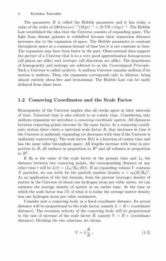
1.2 Comoving Coordinates and the Scale Factor
Homogeneity of the Universe implies also all clocks agree in their intervalsof time. Universal time is also refered to as cosmic time. Considering onlyuniform expansion we introduce a comoving coordinate system. All distancesbetween comoving points increase by the same factor. In a comoving coordi-nate system there exists a universal scale factor R, that increases in time ifthe Universe is uniformly expanding (or decreases with time if the Universe isuniformly contracting). The scale factor R(t) is a function of cosmic time andhas the same value throughout space. All lengths increase with time in pro-portion to R, all surfaces in proportion to R2 and all volumes in proportionto R3.
If R0 is the value of the scale factor at the present time and L0 thedistance between two comoving points, the corresponding distance at anyother time t will be L(t) = (L0/R0)R(t). If an expanding volume V containsN particles, we can write for the particle number density n = n0(R/R0)3.As an application of the last formula, from the present (average) density ofmatter in the Universe of about one hydrogen atom per cubic meter, we canestimate the average density of matter at an earlier time. At the time atwhich the scale factor was 1% of what it is today the average matter densitywas one hydrogen atom per cubic centimeter.
Consider now a comoving body at a fixed coordinate distance. Its actualdistance will be proportional to the scale factor, namely L = R× (coordinatedistance). The recession velocity of the comoving body will be proportionalto the rate of increase of the scale factor R, namely V = R × (coordinatedistance). Dividing the two relations, we obtain
V = LR
R, (1.3)
1 An Introduction to the Physics of the Early Universe 5
tHubble time
R(t)
H>0, q<0 H>0, q>0
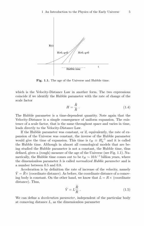
Fig. 1.1. The age of the Universe and Hubble time.
which is the Velocity-Distance Law in another form. The two expressionscoincide if we identify the Hubble parameter with the rate of change of thescale factor
H =R
R. (1.4)
The Hubble parameter is a time-dependent quantity. Note again that theVelocity-Distance is a simple consequence of uniform expansion. The exis-tence of a scale factor, that is the same throughout space and varies in time,leads directly to the Velocity-Distance Law.
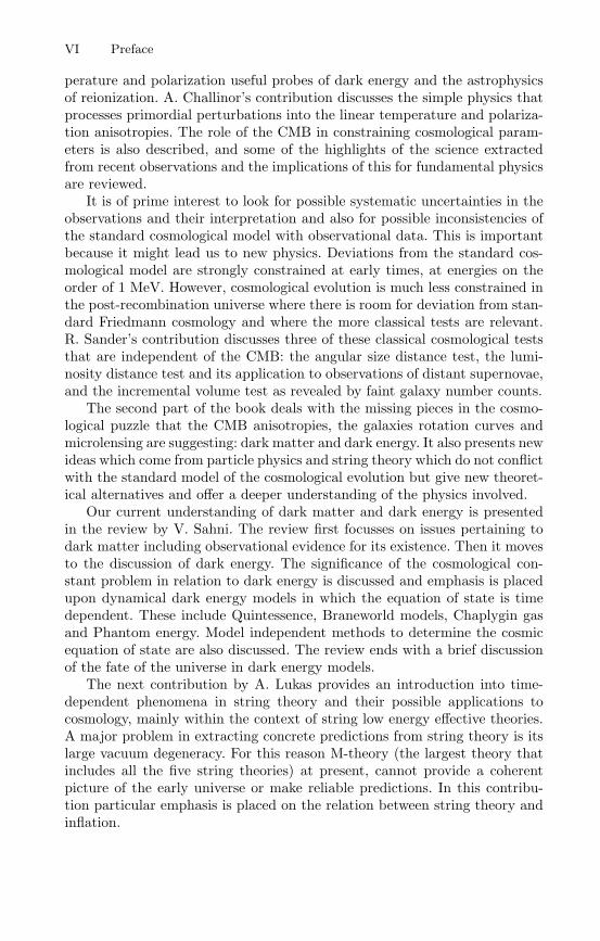
If the Hubble parameter was constant, or if, equivalently, the rate of ex-pansion of the Universe was constant, the inverse of the Hubble parameterwould give the time of expansion. This time is tH ≡ H−1
0 and it is calledthe Hubble time. Although in almost all cosmological models that are be-ing studied the Hubble parameter is not a constant, the Hubble time, thusdefined, gives a (rough) measure of the age of the Universe (see Fig. 1.1). Nu-merically, the Hubble time comes out to be tH ∼ 10h−1 billion years, wherethe dimensionless parameter h is called normalized Hubble parameter and isa number between 0.5 and 0.8.
Acceleration is by definition the rate of increase of the velocity, namelyV = R× (coordinate distance). As before, the coordinate distance of a comov-ing body is constant. On the other hand, we know that L = R× (coordinatedistance). Thus,
V = LR
R. (1.5)
We can define a deceleration parameter , independent of the particular bodyat comoving distance L, as the dimensionless parameter

6 Kyriakos Tamvakis
q ≡ − R
RH2 . (1.6)
When q is positive, it corresponds to deceleration, while, when it is negative, itcorresponds to acceleration and should properly be refered to as accelerationparameter . We can actually classify uniform Universes according to their val-ues of H and q. Such a classification should be called kinematic classification,in contrast to a classification in terms of the curvature, which is a geometricclassification. Kinematically, uniform Universes fall into the following classes:
a) (H > 0, q > 0) expanding and deceleratingb) (H > 0, q < 0) expanding and acceleratingc) (H < 0, q > 0) contracting and deceleratingd) (H < 0, q < 0) contracting and acceleratinge) (H > 0, q = 0) expanding with zero decelerationf) (H < 0, q = 0) contracting with zero decelerationg) (H = 0, q = 0) static.
There is little doubt that only (a), (b) and (e) are possible candidates forour Universe at present. Extrapolating an expanding scenario backwards, wearrive at a very high density state at R → 0. Evidence from CMB radiationsuggests that such a state, described by the suggestive name Big Bang1 couldhave occurred in the Early Universe.
1.3 The Cosmic Microwave Background
The Hubble expansion can be understood as a natural consequence of homo-geneity and isotropy. Nevertheless, an expanding Universe must necessarilyhave a much denser and, therefore, hotter past. Matter in the Early Universe,at times much before the development of any structure, should be viewed asa gas of relativistic particles in thermodynamic equilibrium. The expansioncannot upset the equilibrium, since the characteristic rate of particle pro-cesses is of the order of the characteristic energy, namely T , while the rateof expansion is given by the much smaller scale H ∼ √
GT 2 ∼ (T/MP )T .In order to be convinced for this, one has to invoke the Friedmann equation(see next chapter) and consider the temperature dependence of the energy-density ρ ∼ T 4 characteristic of radiation. The model of the Early Universeas a gas of relativistic matter and electromagnetic radiation in equilibriumwas first considered [4] by G. Gamow and his collaborators R. Alpher and R.Herman for the purpose of explaining nucleosynthesis. As a byproduct, theexistence of relic black body radiation was predicted with wavelength in therange of microwaves corresponding to temperature of a few degrees Kelvin.1 This term was first used by Fred Hoyle in a series of BBC radio talks, published
in The Nature of the Universe (1950). Fred Hoyle was the main proponent of therival Steady State Theory [9] of the Universe.

1 An Introduction to the Physics of the Early Universe 7
This radiation, now known as Cosmic Microwave Background (CMB), wasdiscovered in 1965 by A. Penzias and R. Wilson [5] (see A. Challinor’s con-tribution). The radiation, once extremely hot, has been cooled over billionsof years, redshifted by the expansion of the Universe and has today a tem-perature of a few degrees Kelvin. Black body radiation of a temperature Treaches a maximum at a characteristic wavelength λmax ∼ (1.26 c/kB)T .The average wavelength is of that order. Very accurate observations by theCosmic Background Explorer (COBE) [6] have shown that the intensity ofthe CMB follows the blackbody curve of thermal radiation with a deviationof only one part in 104. Also, after the subtraction of a 24-hour anisotropythat has to do with the motion of the Galaxy at a speed V = 600 km/sec(∆T/T ∼ V/c ∼ 0.01), the radiation is surprising isotropic with only verysmall anisotropies of order ∼ 10−5. Very recently [7], WMAP has pushedthe accuracy with which these anisotropies are determined down to 10−9.These anisotropies, surviving from the time of decoupling, are the imprint ofdensity fluctuations that evolved into galaxies and clusters of galaxies. Theaccuracy with which CMB obeys the Planck spectrum is a very strong phys-ical constraint in favour of an expanding Universe that passes through a hotstage. The COBE estimate of the CMB temperature is
TCMB = 2.725 ± 0.002 oK .
It is possible to get a qualitative idea of the central event related to therelic CMB without going into to much detail. The required quantitative re-lations can easily be met in the framework of specific cosmological models tobe discussed later. We could start at some time in the history of our Universewhen the temperature was greater than 1010 oK. This corresponds roughlyto energy of about 1MeV . The abundant particles, i.e. those with massessmaller than the characteristic energy kB T , apart from the massless photonare the electrons, neutrinos and their antiparticles. The energy is dominatedby the radiation of these particles, which are, at these energies practicallymassless as the photon. Reactions such as e+ e+ γ + γ are in thermody-namic equilibrium, not affected at all by the much slower expansion. The veryimportant effect of the expansion is to lower the temperature, which decreasesinversely proportional to the scale factor. No qualitative change occurs untilthe temperature drops below the characteristic threshold energy kB T ∼ mec
2
at which photons can achieve electron-positron pair creation. Below that tem-perature all electrons and positrons disappear from the plasma. The photonradiation decouples and the Universe becomes essentially transparent to it.It is exactly these photons which, redshifted, we observe as CMB.
The Hubble expansion by itself does not provide sufficient evidence fora Big Bang type of Cosmology. It is only after the observation of the Cos-mic Microwave Background and subsequent work on Nucleosynthesis thatthe Big Bang Model was established as the basic candidate for a StandardCosmological Model.
8 Kyriakos Tamvakis
1.4 The Friedmann Models
A Cosmological Model is a (very) simplified model of the Universe with ageometrical description of spacetime and a smoothed-out matter and radia-tion content. The simplest interesting set of cosmological models is providedby the homogeneous and isotropic Friedmann-Lemaitre spacetimes (FL) [8]which are a set of solutions of GR incorporating the Cosmological Principle.The line element of a FL model reads
ds2 = dt2 −R2(t)dσ2 . (1.7)
The spatial line element dσ2 describes a three-dimensional space of constantcurvature independent of time. It is 2
dσ2 = dχ2 + f2(χ)(dθ2 + sin2 θ dφ2) = dχ2 + f2(χ) dΩ2 . (1.8)
These coordinates are comoving. That means that the actual spatial distanceof two points (χ, θ, φ) and (χ0, θ, φ) will be d = R(t)(χ − χ0). There arethree choices for f(χ), each corresponding to a different spatial curvature k.That is the value of the Ricci scalar (to be defined below) calculated fromdσ2 with the scale factor divided out. They are
f(χ) =
sinχ (k = +1) 0 < χ < πχ (k = 0) 0 < χ <∞
sinhχ (k = −1) 0 < χ <∞. (1.9)
The case k = +1 corresponds to a closed spacetime with a spherical spa-tial geometry. The case k = 0 corresponds to an infinite (flat) spacetimewith Euclidean spatial geometry. Finally, the case k = −1 corresponds to anopen spacetime with hyperbolic spatial geometry. Sometimes the Robertson-Walker metric is written in terms of r ≡ f(χ) as
dσ2 =dr2
1 − kr2 + r2dΩ2 .
The above metric comes out as a solution of Einstein’s Equations
Rµν − 12R gµν − Λgµν = 8πGTµν , (1.10)
Rµν is the Riemann Curvature Tensor and R is the Ricci Scalar defined asR = gµνRµν . G stands for Newton’s Constant of Gravitation. The constant Λis called the Cosmological Constant and Tµν is the Matter Energy-MomentumTensor . A usual choice is that of a fluid2 This is the so called Robertson-Walker metric. A more complete name for these
spacetime solutions is Friedmann-Lemaitre-Robertson-Walker or just FLRWmodels.
1 An Introduction to the Physics of the Early Universe 9
T νµ = (−ρ, p, p p) , (1.11)
with ρ the energy density and p the momentum density, related through someEquation of State.
In the framework of the Robertson-Walker metric, light emitted from asource at the point χS at time tS , propagating along a null geodesic dσ2 = 0,taken radial (dΩ2 = 0) without loss of generality, will reach us at χ0 = 0 attime t0 given by ∫ t0
tS
dt
R(t)= χS .
A second signal emitted at tS + δtS will satisfy∫ t0+δt0
tS+δtS
dt
R(t)= χS ⇒ δtS
R(tS)=
δt0R(t0)
.
The ratio of the observed frequencies will be
ω0
ωS=δtSδt0
=R(tS)R(t0)
.
This implies
z ≡ λ0 − λS
λS=R(t0)R(tS)
− 1 ∼ −1 +R(t0)
R(t0) − (t0 − tS)R(t0)
z ∼ (t0 − tS)H(t0) ⇒ z = H d . (1.12)
This is the Hubble Law . The Velocity-Distance Law is a simple consequenceof uniformity, namely
V = d = Rd
R= H d . (1.13)
Inserting the Robertson-Walker metric into Einstein’s Equations, we ar-rive at the two equations
R = −4πG3
(ρ+ 3p)R+Λ
3R (1.14)
(R)2 =8πG
3ρR2 +
Λ
3R2 − k . (1.15)
Multiplying the first of these equations by R and using the second, we arriveat the equivalent pair of two first order equations, namely
ρ+ 3(ρ+ p)R
R= 0 (1.16)
(R
R
)2
=8πG
3ρ+
Λ
3− k
R2 . (1.17)
10 Kyriakos Tamvakis
The first of these equations is the Continuity Equation expressing the con-servation of energy for the comoving volume R3. This interpretation is moretransparent if we write it in the form
d
dt
(4πR3
3ρ
)= p(
4πR3
3
)⇔ dEdt
= pV .
The other equation is purely dynamical and determines the evolution of thescale factor. It is called The Friedmann Equation.
At the present epoch we have to a very good approximation p0 ≈ 0. Wecan write (1.15) and (1.14) in terms of the present Hubble parameter H0 andthe present deceleration parameter q0. It is convenient to introduce a criticaldensity ρc defined as
ρc ≡ 3H2
8πG. (1.18)
At the present time ρc,0 = 1.05 × 10⁻⁵ h2GeV cm−3. The name and themeaning of ρc will become clear shortly. We also introduce the dimensionlessratio
Ω ≡ ρ0ρc
(1.19)
in terms of which the Friedmann equations are written as
k
R20
= H20
(Ω0 − 1 +
Λ
3H20
), q0 =
12Ω0 − Λ
3H20. (1.20)
In the case of vanishing cosmological constant Λ = 0, we have
q0 =12Ω0 ,
k
R20
= H20 (Ω0 − 1) (1.21)
and, thereforeρ0 > ρc,0 ⇒ k = +1ρ0 = ρc,0 ⇒ k = 0ρ0 < ρc,0 ⇒ k = −1 .
(1.22)
Thus, the measurable quantity Ω0 = ρ0/ρc,0 determines the sign of k, i.e.whether the present Universe is a hyperbolic or a spherical spacetime. Notethat for Λ = 0, H0 and q0 determine the spacetime and the present agecompletely.
It is often necessary to distinguish different contributions to the density,like the present-day density of pressureless matter Ωm, that of relativisticparticles Ωr, plus the quantity ΩΛ ≡ Λ/3H2. In addition to these, in modelswith a variable present-day contribution of the vacuum, one can add a termΩv. Thus, in the general case, we have
k
R20
= H20 (Ωm +Ωr +ΩΛ +Ωv − 1) . (1.23)
1 An Introduction to the Physics of the Early Universe 11
1.5 Simple Cosmological Solutions
1.5.1 Empty de Sitter Universe
In the case of the absence of matter (ρ = p = 0) and for k = 0, the Einstein-Friedmann equations take the very simple form
H2 =Λ
3(1.24)
q = − Λ
3H2 = −1 . (1.25)
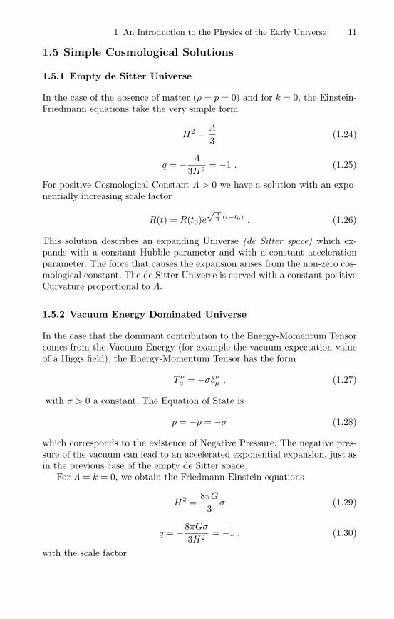
For positive Cosmological Constant Λ > 0 we have a solution with an expo-nentially increasing scale factor
R(t) = R(t0)e√
Λ3 (t−t0) . (1.26)
This solution describes an expanding Universe (de Sitter space) which ex-pands with a constant Hubble parameter and with a constant accelerationparameter. The force that causes the expansion arises from the non-zero cos-mological constant. The de Sitter Universe is curved with a constant positiveCurvature proportional to Λ.
1.5.2 Vacuum Energy Dominated Universe
In the case that the dominant contribution to the Energy-Momentum Tensorcomes from the Vacuum Energy (for example the vacuum expectation valueof a Higgs field), the Energy-Momentum Tensor has the form
T νµ = −σδνµ , (1.27)
with σ > 0 a constant. The Equation of State is
p = −ρ = −σ (1.28)
which corresponds to the existence of Negative Pressure. The negative pres-sure of the vacuum can lead to an accelerated exponential expansion, just asin the previous case of the empty de Sitter space.
For Λ = k = 0, we obtain the Friedmann-Einstein equations
H2 =8πG
3σ (1.29)
q = −8πGσ3H2 = −1 , (1.30)
with the scale factor
12 Kyriakos Tamvakis
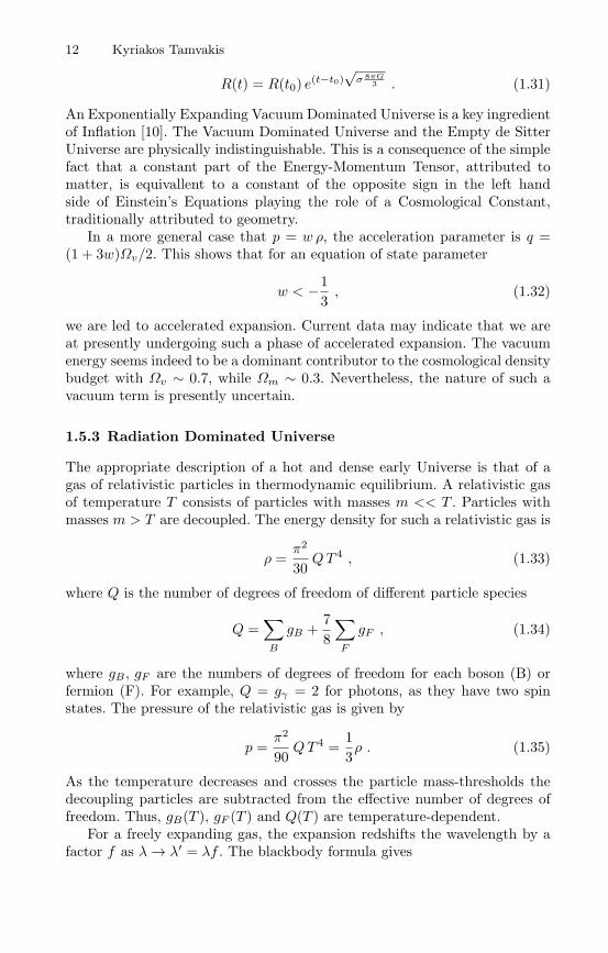
R(t) = R(t0) e(t−t0)√
σ 8πG3 . (1.31)
An Exponentially Expanding Vacuum Dominated Universe is a key ingredientof Inflation [10]. The Vacuum Dominated Universe and the Empty de SitterUniverse are physically indistinguishable. This is a consequence of the simplefact that a constant part of the Energy-Momentum Tensor, attributed tomatter, is equivallent to a constant of the opposite sign in the left handside of Einstein’s Equations playing the role of a Cosmological Constant,traditionally attributed to geometry.
In a more general case that p = w ρ, the acceleration parameter is q =(1 + 3w)Ωv/2. This shows that for an equation of state parameter
w < −13, (1.32)
we are led to accelerated expansion. Current data may indicate that we areat presently undergoing such a phase of accelerated expansion. The vacuumenergy seems indeed to be a dominant contributor to the cosmological densitybudget with Ωv ∼ 0.7, while Ωm ∼ 0.3. Nevertheless, the nature of such avacuum term is presently uncertain.
1.5.3 Radiation Dominated Universe
The appropriate description of a hot and dense early Universe is that of agas of relativistic particles in thermodynamic equilibrium. A relativistic gasof temperature T consists of particles with masses m << T . Particles withmasses m > T are decoupled. The energy density for such a relativistic gas is
ρ =π2
30QT 4 , (1.33)
where Q is the number of degrees of freedom of different particle species
Q =∑
B
gB +78
∑
F
gF , (1.34)
where gB , gF are the numbers of degrees of freedom for each boson (B) orfermion (F). For example, Q = gγ = 2 for photons, as they have two spinstates. The pressure of the relativistic gas is given by
p =π2
90QT 4 =
13ρ . (1.35)
As the temperature decreases and crosses the particle mass-thresholds thedecoupling particles are subtracted from the effective number of degrees offreedom. Thus, gB(T ), gF (T ) and Q(T ) are temperature-dependent.
For a freely expanding gas, the expansion redshifts the wavelength by afactor f as λ → λ′ = λf . The blackbody formula gives
1 An Introduction to the Physics of the Early Universe 13∫dλ
λ5
1e2π/λT − 1
∝ T 4 ⇒ f4∫dλ′
λ′51
e2πf/λ′T − 1∝ T 4 ,
which implies that T ′T = λ
λ′ = RR′ . The relation between temperature and the
scale factor is,T R = const. (1.36)
The Friedmann equation, for Λ = k = 0 gives
H2 =8πG
3ρ =
8π3Q
90T 4 . (1.37)
Note that even if Λ or k were present, they would be irrelevant in early times,when R is small, comparing to the radiation term ρ ∝ R−4. At late times thesituation is reversed and they are more important than the radiation term.From (1.36), (1.37) we obtain
R
R= − T
T=C2
2T 2 ,
with C ≡
32π3Q90
1/4. Taking the initial time t0 = 0 to be a time of infinite
temperature T (0) → ∞ and, therefore, vanishing scale factor R(0) → 0, weget
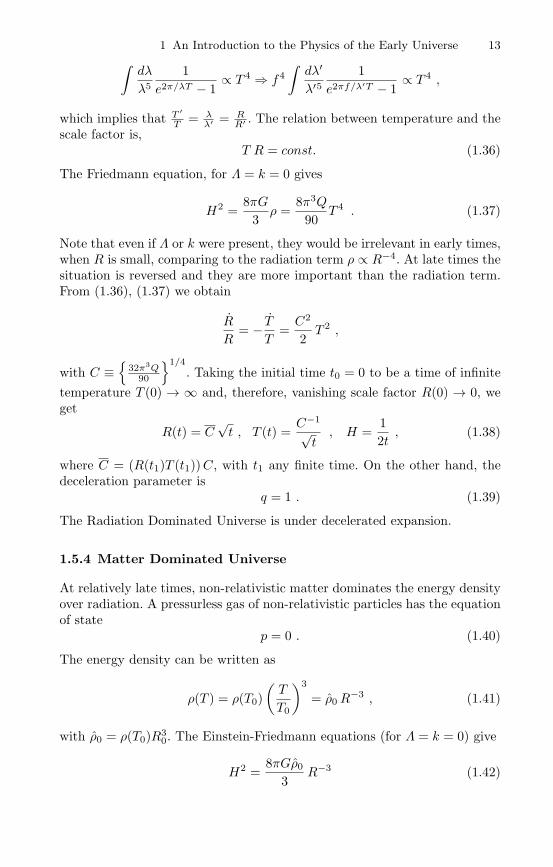
R(t) = C√t , T (t) =
C−1√t, H =
12t, (1.38)
where C = (R(t1)T (t1))C, with t1 any finite time. On the other hand, thedeceleration parameter is
q = 1 . (1.39)
The Radiation Dominated Universe is under decelerated expansion.
1.5.4 Matter Dominated Universe
At relatively late times, non-relativistic matter dominates the energy densityover radiation. A pressurless gas of non-relativistic particles has the equationof state
p = 0 . (1.40)
The energy density can be written as
ρ(T ) = ρ(T0)(T
T0
)3
= ρ0R−3 , (1.41)
with ρ0 = ρ(T0)R30. The Einstein-Friedmann equations (for Λ = k = 0) give
H2 =8πGρ0
3R−3 (1.42)
14 Kyriakos Tamvakis
andq =
12. (1.43)
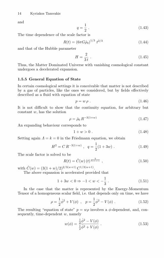
The time dependence of the scale factor is
R(t) = (6πGρ0)1/3
t2/3 (1.44)
and that of the Hubble parameter
H =23 t. (1.45)
Thus, the Matter Dominated Universe with vanishing cosmological constantundergoes a decelerated expansion.
1.5.5 General Equation of State
In certain cosmological settings it is conceivable that matter is not describedby a gas of particles, like the ones we considered, but by fields effectivelydescribed as a fluid with equation of state
p = w ρ . (1.46)
It is not difficult to show that the continuity equation, for arbitrary butconstant w, has the solution
ρ = ρ0R−3(1+w) (1.47)
An expanding behaviour corresponds to
1 + w > 0 . (1.48)
Setting again Λ = k = 0 in the Friedmann equation, we obtain
H2 = C R−3(1+w) , q =12(1 + 3w) . (1.49)
The scale factor is solved to be
R(t) = C(w) (t)2
3(w+1) , (1.50)
with C(w) = (3(1 + w)/2)2/3(w+1) C1/3(w+1).The above expansion is accelerated provided that
1 + 3w < 0 ⇒ −1 < w < −13. (1.51)
In the case that the matter is represented by the Energy-MomentumTensor of a homogeneous scalar field, i.e. that depends only on time, we have
ρ =12φ2 + V (φ) , p =
12φ2 − V (φ) . (1.52)
The resulting “equation of state” p = wρ involves a φ-dependent, and, con-sequently, time-dependent w, namely
w(φ) =12 φ
2 − V (φ)12 φ
2 + V (φ). (1.53)
1 An Introduction to the Physics of the Early Universe 15
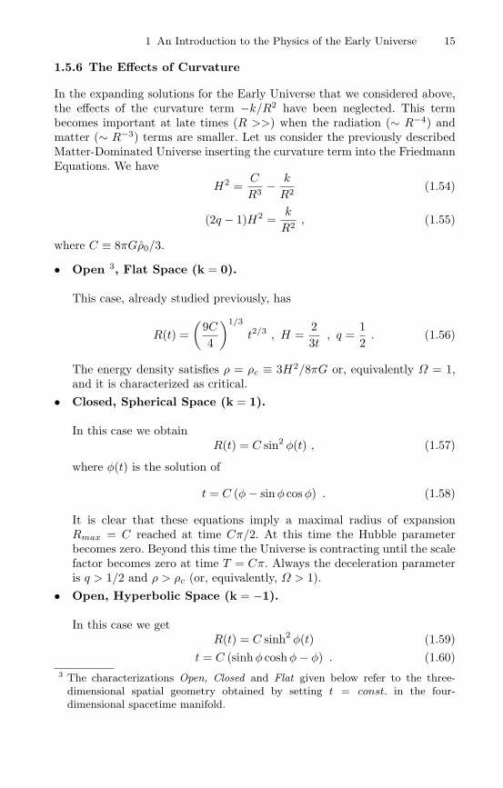
1.5.6 The Effects of Curvature
In the expanding solutions for the Early Universe that we considered above,the effects of the curvature term −k/R2 have been neglected. This termbecomes important at late times (R >>) when the radiation (∼ R−4) andmatter (∼ R−3) terms are smaller. Let us consider the previously describedMatter-Dominated Universe inserting the curvature term into the FriedmannEquations. We have
H2 =C
R3 − k
R2 (1.54)
(2q − 1)H2 =k
R2 , (1.55)
where C ≡ 8πGρ0/3.
• Open 3, Flat Space (k = 0).
This case, already studied previously, has
R(t) =(
9C4
)1/3
t2/3 , H =23t, q =
12. (1.56)
The energy density satisfies ρ = ρc ≡ 3H2/8πG or, equivalently Ω = 1,and it is characterized as critical.
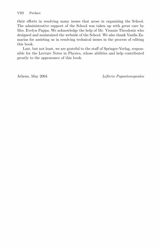
• Closed, Spherical Space (k = 1).
In this case we obtainR(t) = C sin2 φ(t) , (1.57)
where φ(t) is the solution of
t = C (φ− sinφ cosφ) . (1.58)
It is clear that these equations imply a maximal radius of expansionRmax = C reached at time Cπ/2. At this time the Hubble parameterbecomes zero. Beyond this time the Universe is contracting until the scalefactor becomes zero at time T = Cπ. Always the deceleration parameteris q > 1/2 and ρ > ρc (or, equivalently, Ω > 1).
• Open, Hyperbolic Space (k = −1).
In this case we getR(t) = C sinh2 φ(t) (1.59)
t = C (sinhφ coshφ− φ) . (1.60)3 The characterizations Open, Closed and Flat given below refer to the three-
dimensional spatial geometry obtained by setting t = const. in the four-dimensional spacetime manifold.
16 Kyriakos Tamvakis
k=1
k=0
k=−1
t
R
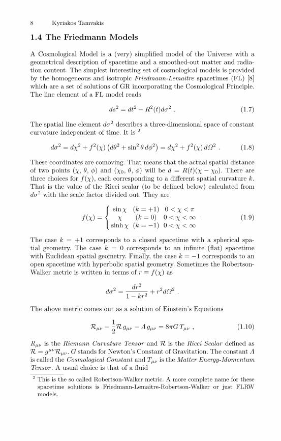
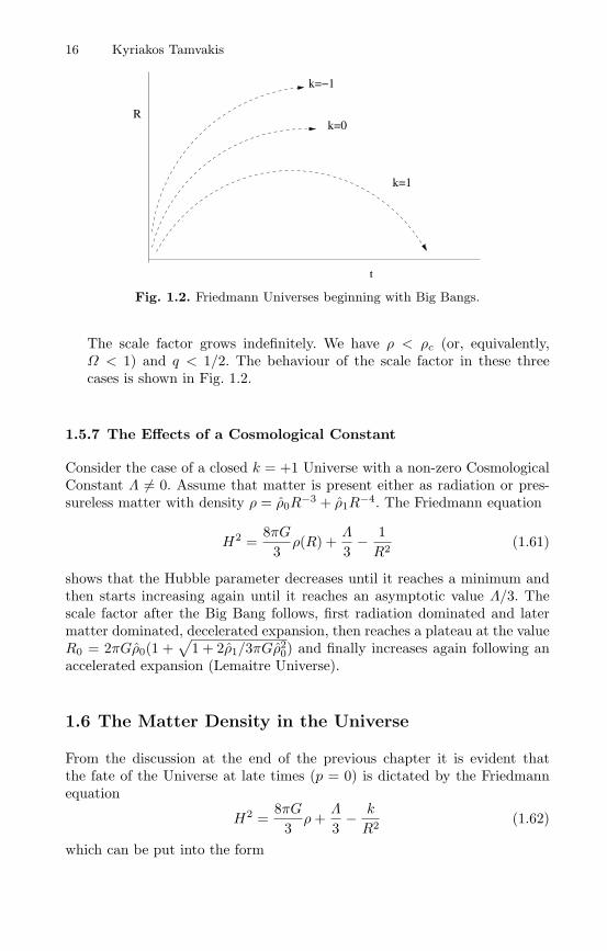
Fig. 1.2. Friedmann Universes beginning with Big Bangs.
The scale factor grows indefinitely. We have ρ < ρc (or, equivalently,Ω < 1) and q < 1/2. The behaviour of the scale factor in these threecases is shown in Fig. 1.2.
1.5.7 The Effects of a Cosmological Constant
Consider the case of a closed k = +1 Universe with a non-zero CosmologicalConstant Λ = 0. Assume that matter is present either as radiation or pres-sureless matter with density ρ = ρ0R−3 + ρ1R−4. The Friedmann equation
H2 =8πG
3ρ(R) +
Λ
3− 1R2 (1.61)
shows that the Hubble parameter decreases until it reaches a minimum andthen starts increasing again until it reaches an asymptotic value Λ/3. Thescale factor after the Big Bang follows, first radiation dominated and latermatter dominated, decelerated expansion, then reaches a plateau at the valueR0 = 2πGρ0(1 +
√1 + 2ρ1/3πGρ20) and finally increases again following an
accelerated expansion (Lemaitre Universe).
1.6 The Matter Density in the Universe
From the discussion at the end of the previous chapter it is evident thatthe fate of the Universe at late times (p = 0) is dictated by the Friedmannequation
H2 =8πG
3ρ+
Λ
3− k
R2 (1.62)
which can be put into the form

1 An Introduction to the Physics of the Early Universe 17
k
R2 = H2 (Ω − 1) , (1.63)
withΩ = Ωm +ΩΛ . (1.64)
having denoted ΩΛ = Λ/3H2. The cosmological constant contribution standsfor a general effective vacuum contribution which could have a, for the mo-ment unknown, dynamical origin. For Ω > 1, the Universe is closed and,in the absence of a cosmological constant, the expansion would change intocontraction. This is not necessarily true in the presence of a non-zero cosmo-logical constant. In the case Ω < 1 the Universe is open and the expansioncontinues forever. This is true also for the critical case Ω = 1.
A lower bound for Ω is supplied by the observed Visible Matter
Ω > 0.03 (1.65)
Arguments based on Primordial Nucleosynthesis support this value. We candenote Ωvm ∼ 0.03. Thus, it seems that most of the mass in the Universeis in an unknown non-baryonic form. This matter is called Dark Matter . Ingeneral, such matter can only be observed indirectly through its gravitation.Doing that, one arrives at an estimate Ωdm ∼ 0.3.
What is the origin of the remaining contribution to Ω? Since it cannot beattributed to matter, visible or dark, it is represented with an effective vac-uum term and has been given the name Dark Energy . For theoretical reasons(i.e. Inflation), the value Ω = 1 is particularly attractive. In that case, theDark Energy contribution is Ωde ∼ 0.7. This estimate is supported by currentdata[11][12]. In particular, current data support the value ΩΛ = Λ/3H2
0 ∼ 0.7or Λ ∼ O(10−56) cm−2. The estimated small cosmological constant is some-times represented by a scale Λ
4= Λ/M2
P ∼ (10−3 eV )4.Thus, in the case of critical density, the various contributions are
Ωvm ∼ 0.03 , Ωdm ∼ 0.27 , Ωde ∼ 0.7 . (1.66)
Although it seems unavoidable, it is surprising that at least 90% of the matterin the Universe is of unknown form.
1.7 The Standard Cosmological Model
The present Universe seems to be described by a Matter Dominated Fried-mann model (p = 0) with a possible vacuum contribution in order to accountfor acceleration. For any time smaller than 104 years from the beginning thedominant part of the energy density was relativistic matter (electromagneticradiation, neutrinos, etc). Thus, the Universe corresponded to a RadiationDominated Friedmann model (p = ρ/3). The relativistic gas description isvalid down to times t ∼ 10−10 sec, corresponding to energies of the order

18 Kyriakos Tamvakis
of 100GeV . For smaller times, or larger energies, the description dependson the assumed theoretical framework beyond [13] the Standard Model ofParticle Physics. If a Quantum Field Theory description of Particle Physicsremains valid up to energies of the order of 1018GeV , then, the relativisticgas description of the Early Universe can be extrapolated down to times ofthe order of 10−42 sec.
1.7.1 Thermal History
During the Radiation Dominated epoch the Friedmann equation is H2 ∼8πGρ/3, since the curvature term is irrelevant at small values of the scalefactor. Thus, the energy density has the critical value
ρ ∼ 3H2
8πG= ρc . (1.67)
The solution (1.38), for each interval of constant effective number of degreesof freedom Q(T ), gives
T (t) =C−1√t, H =
12t
, ρ =3
32πGt2, (1.68)
with
C ≡
16π3QG
45
1/4
. (1.69)
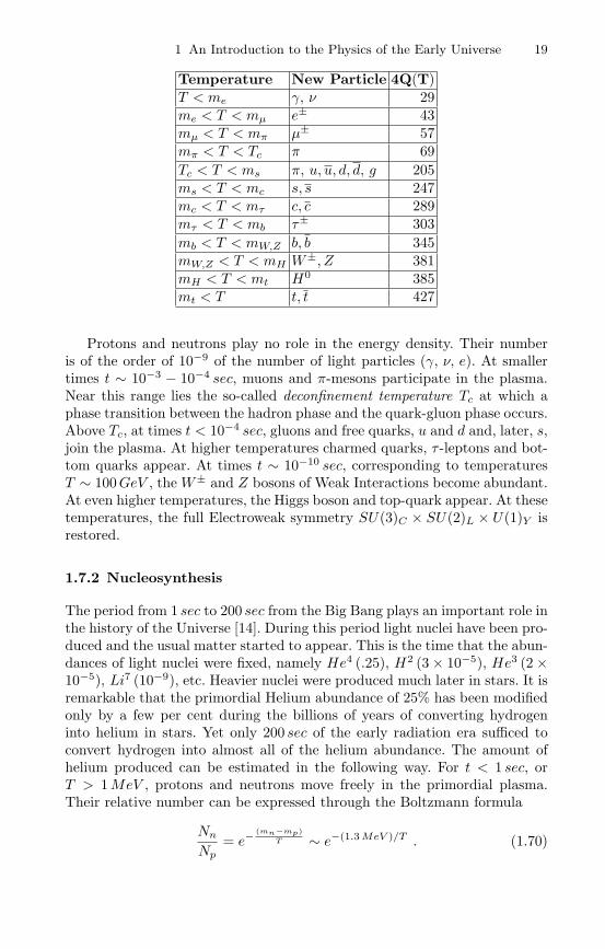
The value of Q(T ) at any given temperature depends on the Particle Physicsmodel valid in the given temperature/energy range. In the following table wegive the values of Q(T ) up to temperatures of O(100GeV ) in the frameworkof the SU(3)C × SU(2)L × U(1)Y Standard Model.
We assume that the relativistic gas is in a state of thermodynamic equi-librium. This is a reasonable assumption since the rate of expansion is muchsmaller than the rate of interactions that can restore the equilibrium. Therate of these interactions is given by the cross section σ ∝ T−2 ∝ t times theparticle number density n ∝ T 3 ∝ t−3/2. Thus, the rate of reactions goes asσn ∼ t−1/2, while the rate of expansion goes as H = 1/2t, guaranteeing thatσn > H as the Universe expands and cools down.
Let us now attempt a bottom-up description of the expansion startingfrom the relatively late time of t ∼ 1 sec, equivalent to T ∼ 1MeV ∼ 1010Kand move backwards in time. Below 1MeV , the plasma consists of photonsand neutrinos. At temperatures T ∼ 1MeV > me electron-positron pairsshould appear thanks to the process
γ + γ e− + e+ .
1 An Introduction to the Physics of the Early Universe 19
Temperature New Particle 4Q(T)T < me γ, ν 29me < T < mµ e± 43mµ < T < mπ µ± 57mπ < T < Tc π 69Tc < T < ms π, u, u, d, d, g 205ms < T < mc s, s 247mc < T < mτ c, c 289mτ < T < mb τ± 303mb < T < mW,Z b, b 345mW,Z < T < mH W±, Z 381mH < T < mt H0 385mt < T t, t 427
Protons and neutrons play no role in the energy density. Their numberis of the order of 10−9 of the number of light particles (γ, ν, e). At smallertimes t ∼ 10−3 − 10−4 sec, muons and π-mesons participate in the plasma.Near this range lies the so-called deconfinement temperature Tc at which aphase transition between the hadron phase and the quark-gluon phase occurs.Above Tc, at times t < 10−4 sec, gluons and free quarks, u and d and, later, s,join the plasma. At higher temperatures charmed quarks, τ -leptons and bot-tom quarks appear. At times t ∼ 10−10 sec, corresponding to temperaturesT ∼ 100GeV , theW± and Z bosons of Weak Interactions become abundant.At even higher temperatures, the Higgs boson and top-quark appear. At thesetemperatures, the full Electroweak symmetry SU(3)C × SU(2)L × U(1)Y isrestored.
1.7.2 Nucleosynthesis
The period from 1 sec to 200 sec from the Big Bang plays an important role inthe history of the Universe [14]. During this period light nuclei have been pro-duced and the usual matter started to appear. This is the time that the abun-dances of light nuclei were fixed, namely He4 (.25), H2 (3 × 10⁻⁵), He3 (2 ×10⁻⁵), Li7 (10−9), etc. Heavier nuclei were produced much later in stars. It isremarkable that the primordial Helium abundance of 25% has been modifiedonly by a few per cent during the billions of years of converting hydrogeninto helium in stars. Yet only 200 sec of the early radiation era sufficed toconvert hydrogen into almost all of the helium abundance. The amount ofhelium produced can be estimated in the following way. For t < 1 sec, orT > 1MeV , protons and neutrons move freely in the primordial plasma.Their relative number can be expressed through the Boltzmann formula
Nn
Np= e−
(mn−mp)T ∼ e−(1.3 MeV )/T . (1.70)
20 Kyriakos Tamvakis
The equilibrium is maintained by the processes ν+ p e+n, n+ ν p+ e,etc. At a temperature Tf ∼ 0.7MeV , these reactions become too slow and theratio freezes out at the value (Nn/Np)f ∼ 0.16. Thus, there is one neutronto about 5 − 6 protons. Free neutron decay (τ ∼ 15min) is too slow tochange that. Protons and neutrons collide together to form deuterium nucleior deuterons through the process
p+ n→ H2 + γ . (1.71)
The deuterons break apart through the inverse process giving back to theplasma protons and neutrons. Only beyond t ∼ 100 sec the temperaure dropsto a point that it is energetically possible for deuterons to be stable. By thistime that protons and neutrons have been able to combine, the abundance ofneutrons has decreased to about two neutrons in every 14 protons. Out of 16nucleons we get two deuterons and 12 protons. The, now stable, deuteronscan combine and produce a He4 nucleus
H2 +H2 ↔ He4 + γ . (1.72)
Actually, one has to consider all the two-body processes, like p + H2 ↔He3+γ, n+He3 ↔ He4+γ, etc. The whole process is over in roughly 200 sec,and in that time 25 % of matter is converted into helium (four out of sixteennucleons form a heliun nucleus) and the remainder consists predominantly ofprotons. Slight amounts of deuterium, He3 and Li are also produced.
1.8 Problems of Standard Cosmology
The Standard Cosmological Model described in the previous section incorpo-rates GR, CMB, the Hubble law and the light nuclei abundance. Needless tosay that its successes are compatible and intimately connected with the Stan-dard Model of fundamental Particle Physics. Nevertheless, it faces a numberof serious problems having to do mostly with the lack of understanding ofinitial conditions. Modifications are needed, which, however, should leave itssuccesses intact.
1.8.1 The Horizon Problem
The maximum size of a region in which causal relations can be established isgiven by the horizon
rH(t) = R(t)∆χ = R(t)∫ t
0
dt′
R(t′). (1.73)
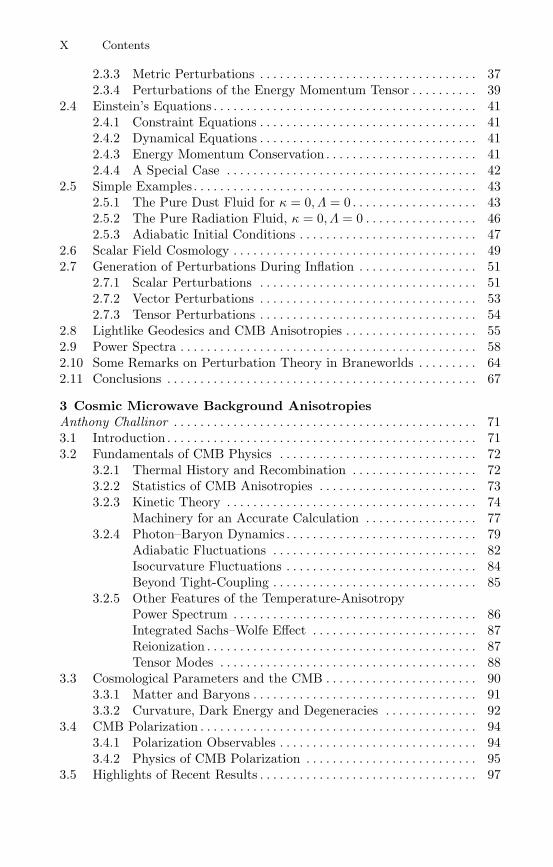
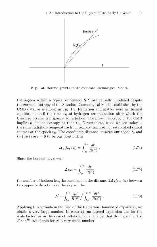
During the Radiation Dominated phase, R(t) ∼ t1/2 and rH(t) = 2t. Fort → 0, rH shrinks much faster than R(t). Thus, at every epoch, most of
1 An Introduction to the Physics of the Early Universe 21
Horizon−>
R(t)
t
Fig. 1.3. Horizon growth in the Standard Cosmological Model.
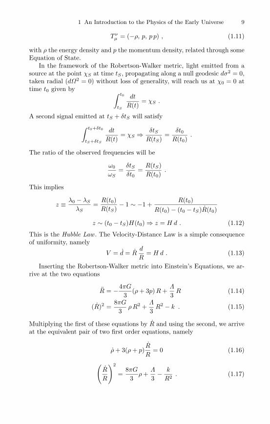
the regions within a typical dimension R(t) are causally unrelated despitethe extreme isotropy of the Standard Cosmological Model established by theCMB data, as is shown in Fig. 1.3. Radiation and matter were in thermalequilibrium until the time tR of hydrogen recombination after which theUniverse became transparent to radiation. The present isotropy of the CMBimplies a similar isotropy at time tR. Nevertheless, what we see today isthe same radiation-temperature from regions that had not established causalcontact at the epoch tR. The coordinate distance between our epoch t0 andtR (we take r = 0 to be our position), is
∆χ(t0, tR) =∫ t0
tR
dt′
R(t′). (1.74)
Since the horizon at tR was
∆χH =∫ tR
tP
dt′
R(t′)(1.75)
the number of horizon lengths contained in the distance 2∆χ(t0, tR) betweentwo opposite directions in the sky will be
N =∫ t0
tR
dt′
R(t′)
/∫ tR
tP
dt′′
R(t′′). (1.76)
Applying this formula in the case of the Radiation Dominated expansion, weobtain a very large number. In contrast, an altered expansion law for thescale factor, as in the case of inflation, could change that dramatically. ForR ∼ eHt, we obtain for N a very small number.
22 Kyriakos Tamvakis
This is the so-called horizon problem of the Standard Cosmological Model.This problem is solved and the observed homogeneity and isotropy is ex-plained in the framework of Inflation which predicts a period of exponentialgrowth for the Universe.
1.8.2 The Coincidence Puzzle and the Flatness Problem
The Friedmann equation for the present epoch has the form
H20 =
8πG3ρ0 − k
R20
+Λ
3. (1.77)
Observations indicate that all three terms of the right hand side can beroughly of the same order of magnitude
8πG3H2
0ρ0 ∼ |k|
R20H
20
∼ Λ
3H20
∼ O(1) . (1.78)
At very early times these terms are of greatly different magnitudes. Sinceρ ∝ R−4, this term dominates over the others which become relevant atvery late times. This very near balance of the three different terms seemscoincidentally very beneficial for our existence and for the existence of theworld around us. For instance, a balance for the first two terms only, fora k = +1 model would be disastrous. In a few Planck-times4 the Universewould collapse. On the other hand, if we have a balance of these two termsin a k = −1 Universe, the resulting expansion would be so rapid that atthe present epoch Ω would be catastrophically small. The coincidence ofthe magnitudes of the different terms is often refereed to as the CoincidencePuzzle.
The balance between the different terms can be best formulated in termsof the Entropy of the Universe. During the Radiation Dominated epoch theentropy density s and the entropy S of a comoving volume R3 are given by
s =2π2Q
45T 3 , S ≡ sR3 =
2π2Q
45(RT )3 . (1.79)
Estimating the present time entropy density from the background of photonsand neutrinos as s0 ∼ nγ ∼ 103 cm−3, we obtain for the entropy the hugenumber
S ∼ 1087 . (1.80)
This number is an initial condition of the Standard Cosmological Model.The fact that there are so much more photons than baryons is somethingdetermined at the beginning.4 The characteristic scale of gravitation, Newton’s gravitational constant G defines
a characteristic mass, the Planck mass MP ∼ 1018GeV , a characteristic length,the Planck length, and a characteristic time, the Planck time.
1 An Introduction to the Physics of the Early Universe 23
Rewriting the Friedman equation in terms of temperature and entropy,we obtain (
T
T
)2
=(
4π3QG
45
)T 4 − k
S2/3
(2π2Q
45
)2/3
. (1.81)
It is clear that the curvature term at high temperature is negligible sinceS is a large number. The Friedmann equation can also be written as (Λ isnegligible at early times)
H2R2|1 −Ω| = |k| ⇒ |1 −Ω|Ω
=1S2/3
(45
2Qπ2
)1/3 12πGT 2 . (1.82)
Inserting numbers, one finds
|1 −Ω|Ω
∼ 10−59(MP
T
)2
. (1.83)
This shows in a dramatic way that Ω must have been terribly close to 1 atearly epochs. For instance
T = 1MeV → |1 −Ω|Ω
≤ 10−15
T = 1014GeV → |1 −Ω|Ω
≤ 10−49 .
This feature of the Standard Cosmological Model, that Ω is close to 1 atall times, is called the Flatness Problem or, sometimes, the Entropy Problem,referring to the large value of the entropy. It is not a problem in an ordinarysense. It relates however the specific properties of our present Universe torather special initial data, like the very large value of the entropy, or havingΩ ∼ 1 at early times. A theory of the Early Universe that could start with Sof order 1 and arrive, via physical processes, to the present number, would beconsidered an improvement because it would not require very specific initialdata.
1.9 Phase Transitions in the Early Universe
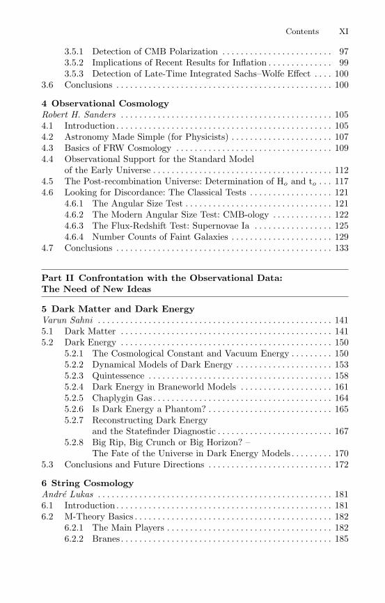
The SU(3)C × SU(2)L × U(1)Y Standard Model of Strong and Electroweakinteractions incorporates the concept of Spontaneous Symmetry Breaking ac-cording to which, although, the Laws of Nature are symmetric under a given(local) gauge symmetry, the vacuum state is not. As a result, the vacuumexpectation values of certain operators in the theory violate the symmetry.The way this is achieved in the Standard Model is through the vacuum ex-pectation value of a scalar (Higgs) field that is an SU(2)L-doublet and carriesweak hypercharge. In the broken SU(3)C × U(1)em vacuum three out of the

24 Kyriakos Tamvakis
0.5 1 1.5 2 2.5
-2
-1
1
2
3
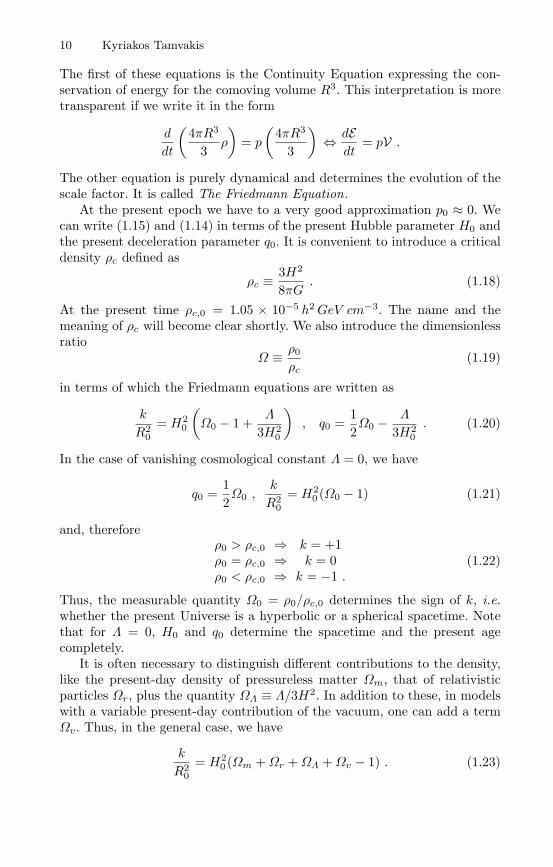
Fig. 1.4. Finite Temperature Effective Potential.
four gauge bosons (W±, Z0) of SU(2)L × U(1)Y obtain a mass, while thefourth (photon) remains massless, corresponding to the intact electromag-netic U(1)em gauge interaction.
In the Early Universe matter corresponds to a system in thermodynamicequilibrium with a heat bath. The thermodynamics of this system is de-scribed by the Hamiltonian of the SU(3)C × SU(2)L × U(1)Y gauge fieldtheory. The vacuum energy of the system is determined by the minimizationof the Free Energy, roughly corresponding to the so-called Effective Poten-tial, which depends on the temperature. At very high temperatures, the globalvacuum state is the symmetric one, in contrast to low temperatures, wherethe global vacuum is the broken one. As the Universe cools down during theRadiation-Dominated epoch it makes a transition from the high temperaturesymmetric phase to the broken low temperature phase, or it undergoes aphase transition. This is shown in Fig. 1.4 where the effective potential atfinite temperature is plotted in terms of the Higgs field vev. This behaviouris in agreement with what happens in certain condensed matter systems. Forexample, a ferromagnet, when heated loses its magnetism, while at zero tem-perature it is characterized by a non-vanishing magnetization that breaksrotational symmetry. A more appropriate analogue is that of the phase tran-sition from water to ice. Normally, the water-ice phase transition occurs atthe freezing point of 00C. Nevertheless, undisturbed pure water supercoolsto a temperature lower than the freezing point before it transforms into ice.When the transition finally occurs, after the supercooling period, the Uni-verse is reheated due to the release of the false vacuum latent heat. Dependingon the details of the theory, symmetry breaking will occur via a first orderphase transition in which the field tunnels through a potential barrier, or viaa second order phase transition in which the field evolves smoothly from onestate to the other.
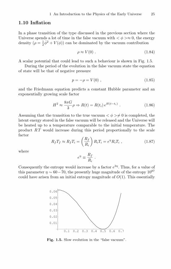
1 An Introduction to the Physics of the Early Universe 25
1.10 Inflation
In a phase transition of the type discussed in the previous section where theUniverse spends a lot of time in the false vacuum with < φ >≈ 0, the energydensity (ρ = 1
2 φ2 + V (φ)) can be dominated by the vacuum contribution
ρ ≈ V (0) . (1.84)
A scalar potential that could lead to such a behaviour is shown in Fig. 1.5.During the period of the evolution in the false vacuum state the equation
of state will be that of negative pressure
p = −ρ = V (0) , (1.85)
and the Friedmann equation predicts a constant Hubble parameter and anexponentially growing scale factor
H2 ≈ 8πG3ρ⇒ R(t) = R(ti) eH(t−ti) . (1.86)
Assuming that the transition to the true vacuum < φ >= 0 is completed, thelatent energy stored in the false vacuum will be released and the Universe willbe heated up to a temperature comparable to the initial temperature. Theproduct RT would increase during this period proportionally to the scalefactor
RfTf ≈ RfTi =(Rf
Ri
)RiTi = eηRiTi , (1.87)
whereeη ≡ Rf
Ri.
Consequently the entropy would increase by a factor e3η. Thus, for a value ofthis parameter η ∼ 60−70, the presently huge magnitude of the entropy 1087
could have arisen from an initial entropy magnitude of O(1). This essentially
0.1 0.2 0.3 0.4 0.5 0.6 0.7
0.01
0.02
0.03
0.04
0.05
0.06
Fig. 1.5. Slow evolution in the “false vacuum”.
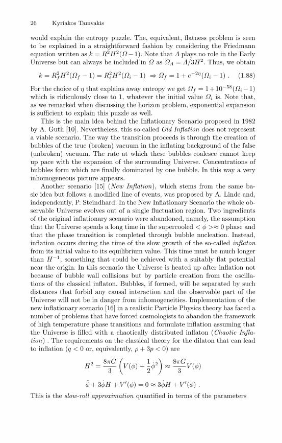
26 Kyriakos Tamvakis
would explain the entropy puzzle. The, equivalent, flatness problem is seento be explained in a straightforward fashion by considering the Friedmannequation written as k = R2H2(Ω−1). Note that Λ plays no role in the EarlyUniverse but can always be included in Ω as ΩΛ = Λ/3H2. Thus, we obtain
k = R2fH
2(Ωf − 1) = R2iH
2(Ωi − 1) ⇒ Ωf = 1 + e−2η(Ωi − 1) . (1.88)
For the choice of η that explains away entropy we get Ωf = 1+10−58(Ωi −1)which is ridiculously close to 1, whatever the initial value Ωi is. Note that,as we remarked when discussing the horizon problem, exponential expansionis sufficient to explain this puzzle as well.
This is the main idea behind the Inflationary Scenario proposed in 1982by A. Guth [10]. Nevertheless, this so-called Old Inflation does not representa viable scenario. The way the transition proceeds is through the creation ofbubbles of the true (broken) vacuum in the inflating background of the false(unbroken) vacuum. The rate at which these bubbles coalesce cannot keepup pace with the expansion of the surrounding Universe. Concentrations ofbubbles form which are finally dominated by one bubble. In this way a veryinhomogeneous picture appears.
Another scenario [15] (New Inflation), which stems from the same ba-sic idea but follows a modified line of events, was proposed by A. Linde and,independently, P. Steindhard. In the New Inflationary Scenario the whole ob-servable Universe evolves out of a single fluctuation region. Two ingredientsof the original inflationary scenario were abandoned, namely, the assumptionthat the Universe spends a long time in the supercooled < φ >≈ 0 phase andthat the phase transition is completed through bubble nucleation. Instead,inflation occurs during the time of the slow growth of the so-called inflatonfrom its initial value to its equilibrium value. This time must be much longerthan H−1, something that could be achieved with a suitably flat potentialnear the origin. In this scenario the Universe is heated up after inflation notbecause of bubble wall collisions but by particle creation from the oscilla-tions of the classical inflaton. Bubbles, if formed, will be separated by suchdistances that forbid any causal interaction and the observable part of theUniverse will not be in danger from inhomogeneities. Implementation of thenew inflationary scenario [16] in a realistic Particle Physics theory has faced anumber of problems that have forced cosmologists to abandon the frameworkof high temperature phase transitions and formulate inflation assuming thatthe Universe is filled with a chaotically distributed inflaton (Chaotic Infla-tion) . The requirements on the classical theory for the dilaton that can leadto inflation (q < 0 or, equivalently, ρ+ 3p < 0) are
H2 =8πG
3
(V (φ) +
12φ2)
≈ 8πG3V (φ)
φ+ 3φH + V ′(φ) = 0 ≈ 3φH + V ′(φ) .
This is the slow-roll approximation quantified in terms of the parameters
1 An Introduction to the Physics of the Early Universe 27
ε(φ) ≡ 116πG
(V ′
V
)2
<< 1 , |η(φ)| ≡ 18πG
∣∣∣∣V ′′
V
∣∣∣∣ << 1 .
Note that the last two conditions (slow-roll conditions) are necessary but notsufficient. The slow-roll approximation requires φ to satisfy 3Hφ ∼ −V ′. Theamount of inflation is N = ln R(tend)
R(t) ∼ 8πG∫ φ
φenddφ V
V ′ ..The historical motivation for inflation arose mostly on the questions con-
cerning the initial conditions required for a Hot Big Bang phase. Nevertheless,in the modern view, by far the most important property of inflation is that itcan generate irregularities in the Universe which may lead to the formationof structure.
1.11 The Baryon Asymmetry in the Universe
Relativistic Quantum Theory predicts that for each elementary particle statethere is another, in general different, state characterizing its antiparticle.Antiparticles have the same spacetime properties (mass, spin) of particles andopposite electric charge. Global quantum numbers, like Baryon and LeptonNumber, are also of opposite sign. Thus, the antiparticle of the electron e isthe positron e+, with positive charge, while the antiparticle of the neutrino isa distinct neutral particle the antineutrino. The two particle wave functionsare related by a symmetry operator
ψe(x) ⇒ C ψe(x) = ψe+(x) .
The term Antimatter refers to the collection of antiparticles. The Universeis almost exclusively filled with matter while existing antimatter is of sec-ondary origin resulting from relativistic collisions of matter. This is true notonly of the antiparticles produced in accelerators but also of the antiparticlesencountered in Cosmic Rays. The evidence against primary forms of anti-matter in the Universe is quite strong. The observed number of Baryons inthe Universe, over the number of photons, is
η =NB
Nγ∼ 10−10 . (1.89)
As first pointed out by A. D. Sakharov [17], the explanation of this asymme-try of matter (Baryon Asymmetry) requires interactions that violate BaryonNumber B, the particle-antiparticle symmetry C (Charge Conjugation) andParity P. In addition, there should be a departure from thermodynamic equi-librium. P and CP non-conservation is a well established fact of the Stan-dard Model. Baryon violation can be found either in Grand Unified Theories(GUTs) or in the non-perturbative sector of the Standard Model. The lastrequirement can be realized in the expanding Universe where the various in-teractions come in and out of equilibrium. The oldest proposed scenario is

28 Kyriakos Tamvakis
that of the out of equilibrium decays of superheavy Higgs bosons of GUTs[18]. Another scenario uses the non-perturbative effects (sphalerons) of theStandard Model and generates the Baryon Asymmetry at the Electroweakscale [19]. Since B + L is conserved by these modes, it is possible to generatefirst a Lepton Asymmetry by the out of equilibrium decay of a superheavyright-handed neutrino [20] (Leptogenesis).
Acknowledgements
The author wishes to thank the organizing committee of the 2nd AegeanSummer School on the Early Universe for inviting him and giving him theopportunity to present the above introduction to the Cosmology of the EarlyUniverse. The author also acknowledges the financial support of the EURTN “Supersymmetry and the Early Universe”, contract No. HPRN-CT-2000-00152.
References
1. S. Weinberg, Gravitation and Cosmology , J. Wiley and Sons (1972);P. J. E. Peebles, Principles of Physical Cosmology , Princeton University Press(1993);G. Borner, The Early Universe: Facts and Fiction, Springer-Verlag (1988);E. W. Kolb and M. S. Turner, The Early Universe, Addison-Wesley (1990).
2. C. W. Misner, K. S. Thorne and J. A. Wheeler, Gravitation, W. H. Freeman& Co. (1973);L. D. Landau and E. M. Lifshitz, The Classical Theory of Fields, PergamonPress, 4th edition (1979);R. M. Wald, General Relativity , Univ. of Chicago Press (1984);W. Rindler Essential Relativity , Van Nostrand Reinhold (1969).
3. E. Hubble and M. L. Humason, Ap. J. 74, 43 (1931).4. R. A. Alpher, R. C. Herman and G. Gamow, Phys. Rev. 73, 803 (1948).5. A. A. Penzias and R. W. Wilson, Ap. J. 142, 419 (1965).6. J. B. Mather et al., Ap. J. 420, 439 (1994);
D. J. Fixen et al., Ap. J. 420, 445 (1994);D. J. Fixen et al., Ap. J. 473, 576 (1996);J. B. Mather et al., Ap. J. 512, 511 (1999).
7. M. R. Nolta et al., astroph/0305097 (March 2003);H. V. Peiris et al., astro-ph/0302225 (Feb. 2003).
8. A. Friedmann, Zeitschrift fur Physik, 10, 377 (1922) and 21, 326 (1924). Bothtranslated in Cosmological Constants, edited by J. Bernstein and G. Feinberg,Columbia Univ. Press (1986).
9. F. Hoyle, Monthly Notices of the Royal Astronomical Society , 108, 372 (1948).10. A. H. Guth, Phys. Rev. D23, 347 (1981).11. A. G. Riess et al., PASP, 116, 1009 (1998);
S. Perlmutter et al., Ap. J. 517, 565 (1999).
1 An Introduction to the Physics of the Early Universe 29
12. D. N. Spergel et al., Ap. J. Suppl. , 148, 175 (2003).13. A. D. Linde, Rep. Prog. Phys. 42, 389 (1979);
K. A. Olive, Phys. Rep. 190, 3345 (1990);C. Vayonakis, Surveys in High Energy Physics 5, 87 (1986).
14. K. A. Olive, G. Steigman and T. P. Walker, Phys. Rep. 333, 389 (2000) andreferences therein.
15. A. D. Linde, Phys. Lett. 108B, 389 (1982);A. Albrecht and P. J. Steindhardt Phys. Rev. Lett. 48, 1220 (1982).
16. A. Linde Particle Physics and Inflationary Cosmology , Harwood (1990);A. R. Liddle and D. H. Lyth, Cosmological Inflation and Large Scale Structure,Cambridge University Press (2000).
17. A. D. Sakharov, JETP Lett. 5, 24 (1967).18. S. Weinberg, Phys. Rev. Lett. 42, 850 (1979).19. V. Kuzmin, V. Rubakov and M. Shaposhnikov Phys. Lett. B155, 36 (1985).20. M. Fukugita and T. Yanagida, Phys. Lett. B174, 45 (1986).

2 Cosmological Perturbation Theory
Ruth Durrer
Universite de Geneve, Departement de Physique Theorique, 24 Quai E. Ansermet,1211 Geneve, Switzerland
Abstract. This is a review on cosmological perturbation theory. After an intro-duction, it presents the problem of gauge transformation. Gauge invariant variablesare introduced and the Einstein and conservation equations are written in termsof these variables. Some examples, especially perfect fluids and scalar fields arepresented in detail. The generation of perturbations during inflation is studied.Lightlike geodesics and their relevance for CMB anisotropies are briefly discussed.Perturbation theory in braneworlds is also introduced.
2.1 Introduction
The idea that the large scale structure of our Universe might have grown outof small initial fluctuations via gravitational instability goes back to Newton(letter to Bentley, 1692 [1]).
The first relativistic treatment of linear perturbations in a Friedmann-Lemaıtre universe was given by Lifshitz (1946) [2]. There he found that thegravitational potential cannot grow within linear perturbation theory and heconcluded that galaxies have not formed by gravitational instability.
Today we know that it is sufficient that matter density fluctuations cangrow. Nevertheless, considerable initial fluctuations with amplitudes of theorder of 10−5 are needed in order to reproduce the cosmic structures observedtoday. These are much larger than typical statistical fluctuations on scales ofgalaxies and we have to propose a mechanism to generate them. Furthermore,the measurements of anisotropies in the cosmic microwave background showthat the amplitude of fluctuations is constant over a wide range of scales, thespectrum is scale independent. As we shall see, standard inflation genericallyproduces such a spectrum of nearly scale invariant fluctuations.
In this review I present gauge invariant cosmological perturbation theory.I shall start by defining gauge invariant perturbation variables. Then I presentthe basic perturbation equations. As examples for the matter equations weshall consider perfect fluids and scalar fields. Then we briefly discuss lightlikegeodesics and CMB anisotropies (this section will be very brief since it iscomplemented by the review on CMB anisotropies by A. Challinor). Finally,I shall make some brief comments on perturbation theory for braneworlds, atopic which is still wide open in my opinion.
R. Durrer, Cosmological Perturbation Theory, Lect. Notes Phys. 653, 31–69 (2005)http://www.springerlink.com/ c© Springer-Verlag Berlin Heidelberg 2005

32 Ruth Durrer
2.2 The Background
I shall not come back to the homogeneous universe which has been discussedin depth by K. Tamvakis. I just specify our notation which is as follows:
A Friedmann-Lemaıtre universe is a homogeneous and isotropic solutionof Einstein’s equations. The hyper-surfaces of constant time are homogeneousand isotropic, i.e. spaces of constant curvature with metric a2(η)γijdx
idxj ,where γij is the metric of a space with constant curvature κ. This metric canbe expressed in the form
γijdxidxj = dr2 + χ2(r)
(dϑ2 + sin2ϑdϕ2) (2.1)
where χ(r) was defined in (1.9) and we have rescaled a(η) such that κ = ±1or 0. (With this normalization the scale factor a has the dimension of a lengthand η and r are dimensionless for κ = 0.) The four-dimensional metric is thenof the form
gµνdxµdxν = −a2(η)dη2 + a2(η)γijdx
idxj . (2.2)
Here η is called the conformal time. The physical or cosmological time is givenby dt = adη.
Einstein’s equations reduce to ordinary differential equations for the func-tion a(η) (with ˙≡ d/dη):
(a
a
)2
+ κ = H2 + κ =8πG
3a2ρ+
13Λa2 (2.3)
(a
a
)·= H = −4πG
3a2 (ρ+ 3p) +
13Λa2 =
(a
a
)−(a
a
)2
, (2.4)
where ρ = −T 00 , p = T i
i (no sum!) and all other components of the energymomentum tensor have to vanish by the requirement of isotropy and homo-geneity. Λ is the cosmological constant. We have introduced H = a/a. TheHubble parameter is defined by
H =da/dt
a=a
a2= H/a .
Energy momentum “conservation” (which is also a consequence of (2.3)and (2.4) due to the contracted Bianchi identity) reads
ρ = −3(a
a
)(ρ+ p) = −3(1 + w)H, (2.5)
where w ≡ p/ρ. Later we will also use c2s ≡ p/ρ. From the definition of w andρ together with (2.5) one finds
w = 3(1 + w)(w − c2s)H . (2.6)
2 Cosmological Perturbation Theory 33
From the Friedmann equations one easily concludes that for κ = Λ = 0 andw =const. the scale factor behaves like a power law,
a ∝ η 21+3w ∝ t 2
3(1+w) . (2.7)
Important examples are
a ∝ ηq with
q = 2 for dust w = 0q = 1 for radiation w = 1/3q = −1 for inflation (or a cosm. const.) w = −1
(2.8)
We also define
Ωρ =(
8πGρa2
3H2
)
η=η0
ΩΛ =Λa2
3H2
∣∣∣∣η=η0
(2.9)
Ωκ =−κH2
∣∣∣∣η=η0
,
where the index 0 indicates the value of a given variable today. Friedmann’sequation (2.3) then requires
1 = Ωρ +ΩΛ +Ωκ. (2.10)
One often also uses Ω = Ωρ +ΩΛ = 1 −Ωκ.
2.3 Gauge Invariant Perturbation Variables
The observed Universe is not perfectly homogeneous and isotropic. Matter isarranged in galaxies and clusters of galaxies and there are large voids in thedistribution of galaxies. Let us assume, however, that these inhomogeneitieslead only to small variations of the geometry which we shall treat in firstorder perturbation theory. For this we define the perturbed geometry by
gµν = gµν + εa2hµν , (2.11)
gµν being the unperturbed Friedmann metric. We conventionally set (absorb-ing the “smallness” parameter ε into hµν)
gµν = gµν + a2hµν , g00 = −a2, gij = a2γij |hµν | 1
Tµν = T
µ
ν + θµν , T
00 = −ρ, T
i
j = pδij |θµν |/ρ 1.
(2.12)
34 Ruth Durrer
2.3.1 Gauge Transformation, Gauge Invariance
The first fundamental problem we want to discuss is the choice of gauge incosmological perturbation theory:
For linear perturbation theory to apply, the spacetime manifold M withmetric g and the energy momentum tensor T of the real, observable universemust be in some sense close to a Friedmann universe, i.e. the manifold Mwith a Robertson–Walker metric g and a homogeneous and isotropic energymomentum tensor T . It is an interesting, non–trivial unsolved problem howto construct ‘the best’ g and T from the physical fields g and T in practice.There are two main difficulties: First, spatial averaging procedures dependon the choice of a hyper–surface of constant time and they do not commutewith derivatives, so that averaged fields g and T will in general not satisfyEinstein’s equations. Secondly, averaging is in practice impossible over super–horizon scales.
Even though we cannot give a constructive prescription, we now as-sume that there exists an averaging procedure which leads to a Friedmannuniverse with spatially averaged tensor fields Q, such that the deviations(Tµν−Tµν)/maxαβ|Tαβ | and (gµν−gµν)/maxαβgαβ are small, and gand T satisfy Friedmann’s equations. Let us call such an averaging procedure‘admissible’. There may be many different admissible averaging procedures(e.g. over different hyper–surfaces) leading to slightly different Friedmannbackgrounds. But since |g − g| is small of order ε, the difference of the twoFriedmann backgrounds must also be small of order ε and we can regard itas part of the perturbation.
We consider now a fixed admissible Friedmann background (g, T ) as cho-sen. Since the theory is invariant under diffeomorphisms (coordinate transfor-mations), the perturbations are not unique. For an arbitrary diffeomorphismφ and its push forward φ∗, the two metrics g and φ∗(g) describe the samegeometry. Since we have chosen the background metric g we only allow dif-feomorphisms which leave g invariant i.e. which deviate only in first orderform the identity. Such an ‘infinitesimal’ diffeomorphism can be representedas the infinitesimal flow of a vector field X, φ = φX
ε . Remember the defini-tion of the flow: For the integral curve γx(s) of X with starting point x, i.e.,γx(s = 0) = x we have φX
s (x) = γx(s). In terms of the vector field X, to firstorder in ε, its pullback is then of the form
φ∗ = id+ εLX
(LX denotes the Lie derivative in direction X 1. The transformation g →φ∗(g) is equivalent to g + εa2h → g + ε(a2h + LX g) + O(ε2), i.e. under1 The Lie derivative is geometrically just the derivative in the direction of the
vector field. To define it in a coordinate independent manner, we consider avector field X and its flux φs(x), i.e. the solution of the equation dxds = X(x)with starting point x. For small enough values of s this is well defined. The Liederivative of a tensor field T is then defined by
2 Cosmological Perturbation Theory 35
an ‘infinitesimal coordinate transformation’ the metric perturbation h trans-forms as
h→ h+ a−2LX g . (2.13)
In the context of cosmological perturbation theory, infinitesimal coordinatetransformations are called ‘gauge transformations’. The perturbation of aarbitrary tensor field Q = Q+ εQ(1) obeys the gauge transformation law
Q(1) → Q(1) + LXQ . (2.14)
Since every vector field X generates a gauge transformation φ = φXε ,
we can conclude that only perturbations of tensor fields with LXQ = 0 forall vector fields X, i.e. with vanishing (or constant) ‘background contribu-tion’ are gauge invariant. This simple result is sometimes referred to as the‘Stewart-Walker Lemma’ [4].
The gauge dependence of perturbations has caused many controversiesin the literature, since it is often difficult to extract the physical meaningof gauge dependent perturbations, especially on super–horizon scales. Thishas led to the development of gauge invariant perturbation theory which weare going to use throughout this review. The advantage of the gauge invari-ant formalism is that the variables used have simple geometric and physicalmeanings and are not plagued by gauge modes. Although the derivation re-quires somewhat more work, the final system of perturbation equations isusually simple and well suited for numerical treatment. We shall also see,that on sub-horizon scales, the gauge invariant matter perturbation variablesapproach the usual, gauge dependent ones. Since one of the gauge invariantgeometrical perturbation variables corresponds to the Newtonian potential,the Newtonian limit can be performed easily.
First we note that since all relativistic equations are covariant (i.e. can bewritten in the form Q = 0 for some tensor field Q), it is always possible toexpress the corresponding perturbation equations in terms of gauge invariantvariables [5, 6, 7].
2.3.2 Harmonic Decomposition of Perturbation Variables
Since the η = const hyper-surfaces are homogeneous and isotropic, it issensible to perform a harmonic analysis: A (spatial) tensor field Q on thesehyper-surfaces can be decomposed into components which transform irre-ducibly under translations and rotations. All such components evolve inde-pendently. For a scalar quantity f in the case κ = 0 this is nothing else thanits Fourier decomposition:
f(x, η) =∫d3kf(k)eikx. (2.15)
LXT = lims→0 (φ∗sT − T ) /s.
Here φ∗s denotes the pullback with the (local) diffeomorphism φs [3].
36 Ruth Durrer
(The exponentials Yk(x) = eikx are the unitary irreducible representations ofthe Euclidean translation group.) For κ = 1 such a decomposition also exists,but the values k are discrete, k2 = (+2) and for κ = −1, they are boundedfrom below, k2 > 1. Of course, the functions Yk are different for κ = 0.
They form the complete orthogonal set of eigenfunctions of the Laplacian,
∆Y(S)k = −k2Y
(S)k . (2.16)
In addition, a tensorial variable (at fixed position x) can be decomposed intoirreducible components under the rotation group SO(3).
For a vector field, this is its decomposition into a gradient and a rotation,
Vi = ∇iϕ+Bi , (2.17)
whereBi
|i = 0 , (2.18)
where we used X|i to denote the three–dimensional covariant derivative ofX. Here ϕ is the spin 0 and B is the spin 1 component of the vector field V.
For a symmetric tensor field we have
Hij = HLγij +(
∇i∇j − 13∆γij
)HT +
12
(H
(V )i|j +H(V )
j|i)
+H(T )ij , (2.19)
whereH
(V )|ii = H(T )i
i = H(T )j
i|j = 0. (2.20)
Here HL and HT are spin 0 components, H(V )i is a spin 1 component and
H(T )ij is a spin 2 component.
We shall not need higher tensors (or spinors). As a basis for vector andtensor modes we use the vector and tensor type eigenfunctions of the La-placian,
∆Y(V )j = −k2Y
(V )j and (2.21)
∆Y(T )ji = −k2Y
(T )ji , (2.22)
where Y (V )j is a transverse vector, Y (V )|j
j = 0 and Y (T )ji is a symmetric trans-
verse traceless tensor, Y (T )jj = Y (T )|i
ji = 0.According to (2.17) and (2.19) we can construct scalar type vectors and
tensors and vector type tensors. To this goal we define
Y(S)j ≡ −k−1Y
(S)|j (2.23)
Y(S)ij ≡ k−2Y
(S)|ij +
13γijY
(S) (2.24)
Y(V )ij ≡ − 1
2k(Y (V )
i|j + Y (V )j|i ) . (2.25)
2 Cosmological Perturbation Theory 37
In the following we shall extensively use this decomposition and write downthe perturbation equations for a given mode k. The decomposition of a vectorfield is then of the form
Bi = BY (S)i +B(V )Y
(V )i . (2.26)
The decomposition of a tensor field is given by (compare (2.19))
Hij = HLY(S)γij +HTY
(S)ij +H(V )Y
(V )ij +H(T )Y
(T )ij . (2.27)
Here B, B(V ), HL, HT , H(V ) and H(T ) are functions of η and k.
2.3.3 Metric Perturbations
Perturbations of the metric are of the form
gµν = gµν + a2hµν . (2.28)
We parameterize them as
hµνdxµdxν = −2Adη2 − 2Bidηdx
i + 2Hijdxidxj , (2.29)
and we decompose the perturbation variables Bi and Hij according to (2.26)and (2.27).
Let us consider the behavior of hµν under gauge transformations. We setthe vector field defining the gauge transformation to
X = T∂η + Li∂i. (2.30)
Using simple identities from differential geometry like LX(df) = d(LXf) and(LXγ)ij = Xi|j +Xj|i, we obtain
LXg = a2[−2(a
aT + T
)dη2 + 2
(Li − T,i
)dηdxi
+(
2a
aTγij + Li|j + Lj|i
)dxidxj
]. (2.31)
Comparing this with (2.29) and using (2.13) we obtain the following be-haviour of our perturbation variables under gauge transformations (we de-compose the vector Li = LY (S)
i + L(V )Y(V )i ):
A → A+a
aT + T (2.32)
B → B − L− kT (2.33)B(V ) → B(V ) − L(V ) (2.34)
HL → HL +a
aT +
k
3L (2.35)
HT → HT − kL (2.36)H(V ) → H(V ) − kL(V ) (2.37)H(T ) → H(T ). (2.38)
38 Ruth Durrer
Two scalar and one vector variable can be set to zero by a cleverly chosengauge transformations.
One often chooses kL = HT and kT = B + L, so that the variables HT
and B vanish. In this gauge (longitudinal gauge), scalar perturbations of themetric are of the form (HT = B = 0):
h(S)µν = −2Ψdη2 − 2Φγijdx
idxj . (2.39)
Ψ and Φ are the so called Bardeen potentials. In a generic gauge they aregiven by
Ψ = A− a
ak−1σ − k−1σ (2.40)
Φ = −HL − 13HT +
a
ak−1σ, (2.41)
with σ = k−1HT − B. A short calculation using (2.32) to (2.36) shows thatΨ and Φ are gauge invariant.
In a Friedmann universe the Weyl tensor vanishes. It therefore is a gaugeinvariant perturbation. For scalar perturbations one finds
C0i0j =
12
[(Ψ + Φ)|ij − 1
3(Ψ + Φ)γij
]. (2.42)
All other components vanish.For vector perturbations it is convenient to set kL(V ) = H(V ) so that
H(V ) vanishes and we have
h(V )µν dx
µdxν = 2σ(V )Y(V )i dηdxi. (2.43)
We shall call this gauge the “vector gauge”. In general σ(V ) = k−1H(V )−B(V )
is gauge invariant2. The Weyl tensor from vector perturbation is given by
C0i0j =
12σ(V )Y
(V )ij (2.44)
C0jlm =
12σ(V )[Y (V )
jl|m − Y (V )jm|l − 1
3γjlY
(V )m|k
k +13γjmY
(V )l|k
k]. (2.45)
Clearly there are no tensorial (spin 2) gauge transformation and hence H(T )ij
is gauge invariant. The expression for the Weyl tensor from tensor perturba-tion is identical to the one for vector perturbation upon replacement of σ(V )
ij
by H(T )ij .
2 Y(V )
ij σ(V ) is the shear of the hyper-surfaces of constant time.

2 Cosmological Perturbation Theory 39
2.3.4 Perturbations of the Energy Momentum Tensor
Let Tµν = T
µ
ν + θµν be the full energy momentum tensor. We define its en-
ergy density ρ and its energy flow 4-vector u as the time-like eigenvalue andeigenvector of Tµ
ν :Tµ
ν uν = −ρuµ, u2 = −1. (2.46)
We then parameterize their perturbations by
ρ = ρ (1 + δ) , u = u0∂t + ui∂i. (2.47)
u0 is fixed by the normalization condition,
u0 =1a(1 −A). (2.48)
We further setui =
1avi = vY (S)i + v(V )Y (V )i. (2.49)
We define Pµν ≡ uµuν + δµν , the projection tensor onto the part of tangent
space normal to u and set the stress tensor
τµν = PµαP
νβ T
αβ . (2.50)
In the unperturbed case we have τ00 = 0, τ i
j = pδij . Including perturba-tions, to first order we still obtain
τ00 = τ0
i = τ i0 = 0. (2.51)
But τ ij contains in general perturbations. We set
τ ij = p
[(1 + πL) δij +Πi
j
], with Πi
i = 0. (2.52)
We decompose Πij as
Πij = Π(S)Y
(S) ij +Π(V )Y
(V ) ij +Π(T )Y
(T ) ij . (2.53)
We shall not derive the gauge transformation properties of these pertur-bation variables in detail, but just state some results which can be obtainedas an exercise (see also [6]):
– Of the variables defined above only the Π(S,V,T ) are gauge invariant; theydescribe the anisotropic stress tensor, Πµ
ν = τµν − 1/3τα
α δµν . They are gauge
invariant due to the Stewart–Walker lemma, since Π = 0. For perfectfluids Πµ
ν = 0.– A second gauge invariant variable is
Γ = πL − c2swδ, (2.54)
where c2s ≡ p/ρ is the adiabatic sound speed and w ≡ p/ρ is the enthalpy.One can show that Γ is proportional to the divergence of the entropy fluxof the perturbations. Adiabatic perturbations are characterized by Γ = 0.
40 Ruth Durrer
– Gauge invariant density and velocity perturbations can be found by com-bining δ, v and v(V )
i with metric perturbations.
We shall use
V ≡ v − 1kHT = v(long) (2.55)
Ds ≡ δ + 3(1 + w)a
a(k−2HT − k−1B) ≡ δ(long) (2.56)
D ≡ δ(long) + 3(1 + w)(a
a
)V
k(2.57)
Dg ≡ δ + 3(1 + w)(HL +
13HT
)= δ(long) − 3(1 + w)Φ (2.58)
V (V ) ≡ v(V ) − 1kH(V ) = v(vec) (2.59)
Ω ≡ v(V ) −B(V ) = v(vec) −B(V ) (2.60)Ω − V (V ) = σ(V ). (2.61)
Here v(long), δ(long) and v(vec)i are the velocity (and density) perturbationsin the longitudinal and vector gauge respectively, and σ(V ) is the metricperturbation in vector gauge (see (2.43)). These variables can be interpretednicely in terms of gradients of the energy density and the shear and vorticityof the velocity field [8].
Here I just want to show that on scales much smaller than the Hubblescale, kη 1, the metric perturbations are much smaller than δ and v andwe can thus “forget them” (which will be important when comparing experi-mental results with calculations in this formalism): The perturbations of theEinstein tensor are given by second derivatives of the metric perturbations.Einstein’s equations yield the following order of magnitude estimate:
O(δT
T
)O (8πGT )︸ ︷︷ ︸
O( aa )2
=O(η−2)
= O(
1η2h+
k
ηh+ k2h
)(2.62)
O(δT
T
)= O (h+ kηh+ (kη)2h
). (2.63)
For kη 1 this gives O(δ, v) = O ( δTT
) O(h). On sub-horizon scales thedifference between δ, δ(long), Dg and D is negligible as well as the differencebetween v and V or v(V ), V (V ) and Ω(V ).
2 Cosmological Perturbation Theory 41
2.4 Einstein’s Equations
We do not derive the first order perturbations of Einstein’s equations. Thiscan be done by different methods, for example with Mathematica. We justwrite down those equations which we shall need later.
2.4.1 Constraint Equations
4πGa2ρD = −(k2 − 3κ)Φ (00)4πGa2(ρ+ p)V = k
((aa
)Ψ + Φ
)(0i)
(scalar) (2.64)
8πGa2(ρ+ p)Ω =12(2κ− k2)σ(V ) (0i) (vector) (2.65)
2.4.2 Dynamical Equations
k2 (Φ− Ψ) = 8πGa2pΠ(S) (scalar) (2.66)
k
(σ(V ) + 2
(a
a
)σ(V )
)= 8πGa2pΠ(V ) (vector) (2.67)
H(T ) + 2(a
a
)H(T ) +
(2κ+ k2)H(T ) = 8πGa2pΠ(T )
ij (tensor) (2.68)
There is a second dynamical scalar equation, which is somewhat cumbersomeand not really needed, since we may use one of the conservation equationsgiven below instead. Note that for perfect fluids, where Πi
j ≡ 0, we haveΦ = Ψ , σ(V ) ∝ 1/a2 and H(T ) obeys a damped wave equation. The dampingterm can be neglected on small scales (over short time periods) when η−2 <∼2κ + k2, and Hij represents propagating gravitational waves. For vanishingcurvature, these are just the sub-horizon scales, kη >∼ 1. For κ < 0, wavesoscillate with a somewhat smaller frequency, ω =
√2κ+ k2, while for κ > 0
the frequency is somewhat larger than k.
2.4.3 Energy Momentum Conservation
The conservation equations, Tµν;ν = 0 lead to the following perturbation equa-
tions
Dg + 3(c2s − w) ( a
a
)Dg + (1 + w)kV + 3w
(aa
)Γ = 0
V +(
aa
) (1 − 3c2s
)V = k
(Ψ + 3c2sΦ
)+ c2
sk1+wDg
+ wk1+w
[Γ − 2
3
(1 − 3κ
k2
)Π]
(scalar) (2.69)
Ωi +(1 − 3c2s
)(a
a
)Ωi =
p
2(ρ+ p)
(k − 2κ
k
)Π
(V )i (vector) (2.70)
42 Ruth Durrer
These can of course also be obtained from the Einstein equations since theyare equivalent to the contracted Bianchi identities. For scalar perturbationswe have 4 independent equations and 6 variables. For vector perturbationswe have 2 equations and 3 variables, while for tensor perturbations we have1 equations and 2 variables. To close the system we must add some matterequations. The simplest prescription is to set Γ = Πij = 0. This matterequation, which describes adiabatic perturbations of a perfect fluid gives usexactly two additional equations for scalar perturbations and one each forvector and tensor perturbations.
Another simple example is a universe with matter content given by ascalar field. We shall discuss this case in the next section. More complicatedexamples are those of several interacting particle species of which some haveto be described by a Boltzmann equation. This is the actual universe at latetimes, say z <∼ 107.
2.4.4 A Special Case
Here we want to rewrite the scalar perturbation equations for a simple butimportant special case. We consider adiabatic perturbations of a perfect fluid.In this case Π = 0 since there are no anisotropic stresses and Γ = 0.Equation (2.66) then implies Φ = Ψ . Using the first equation of (2.64) and(2.58,2.57) to replace Dg in the second of (2.69) by Ψ and V , finally replacingV by (2.64) one can derive a second order equation for Ψ , which is, in thiscase the only dynamical degree of freedom
Ψ + 3H(1 + c2s)Ψ + [(1 + 3c2s)(H2 − κ) − (1 + 3w)H2 + c2sk2]Ψ = 0 . (2.71)
Another interesting case (especially when discussing inflation) is the scalarfield case. There, as we shall see in Sect. 2.6, Π = 0, but in general Γ = 0since δp/δρ = p/ρ. Nevertheless, since this case again has only one dynamicaldegree of freedom, we can express the perturbation equations in terms of onesingle second order equation for Ψ . In Sect. 2.6 we shall find the followingequation for a perturbed scalar field cosmology
Ψ + 3H(1 + c2s)Ψ + [(1 + 3c2s)(H2 − κ) − (1 + 3w)H2 + k2]Ψ = 0 . (2.72)
The only difference between the perfect fluid and scalar field perturbationequation is that the latter is missing the factor c2s in front of the oscillatoryk2 term. Note also that for κ = 0 and w = c2s = constant, the time dependentmass term m2(η) = −(1 + 3c2s)(H2 − κ) + (1 + 3w)H2 vanishes. It is usefulto define also the variable [12]
u = a[4πG(H2 − H + κ)
]−1/2Ψ, (2.73)
which satisfies the equation

2 Cosmological Perturbation Theory 43
u+ (Υk2 − θ/θ)u = 0, (2.74)
where Υ = c2s or Υ = 1 for a perfect fluid or a scalar field backgroundrespectively, and
θ =3H
2a√
H2 − H + κ. (2.75)
Another interesting variable is
ζ ≡ 2(H−1Ψ + Ψ)3(1 + w)
+ Ψ . (2.76)
Using (2.71) and (2.72) respectively one obtains
ζ = −k2 ΥHH2 − HΨ , (2.77)
hence on super horizon scales, k/H 1, this variable is conserved.The evolution of ζ is closely related to the canonical variable v defined by
v = −a√
H2 − H√4πGΥH ζ . (2.78)
which satisfies the equation
v + (Υk2 − z/z)v = 0 , (2.79)
for
z =a√
H2 − H + κΥH . (2.80)
More details on the significance of the canonical variable v will be found inSects. 2.6 and 2.7.
2.5 Simple Examples
We first discuss two simple applications which are important to understandthe CMB anisotropy spectrum.
2.5.1 The Pure Dust Fluid for κ = 0, Λ = 0
We assume the dust to have w = c2s = p = 0 and Π = Γ = 0. (2.71) thenreduces to
Ψ +6ηΨ = 0 , (2.81)
with the general solution
44 Ruth Durrer
Ψ = Ψ0 + Ψ11η5 , (2.82)
with arbitrary constants Ψ0 and Ψ1. Since the perturbations are supposed tobe small initially, they cannot diverge for η → 0, and we have therefore tochoose the growing mode, Ψ1 = 0. Another way to argue is as follows: If themode Ψ1 has to be small already at some early initial time ηin, it will be evenmuch smaller later and may hence be neglected at late times. But also theΨ0 mode is only constant. This fact led Lifshitz who was the first to analyzecosmological perturbations to the conclusions that linear perturbations donot grow in a Friedman universe and cosmic structure cannot have evolvedby gravitational instability [2]. However, the important point to note hereis that, even if the gravitational potential remains constant, matter densityfluctuations do grow on sub-horizon scales and therefore inhomogeneities,structure can evolve on scales which are smaller than the Hubble scale. Tosee that we consider the conservation equations (2.69), (2.66) and the Poissonequation (2.64). For the pure dust case, w = c2s = Π = Γ = 0, they reduce to
Dg = −kV (energy conservation) (2.83)
V +(a
a
)V = kΨ (gravitational acceleration) (2.84)
−k2Ψ = 4πGa2ρ(Dg + 3
(Ψ +
(a
a
)k−1V
))(Poisson), (2.85)
where we have used the relation
D = Dg + 3(1 + w)(
−Φ+(a
a
)k−1V
). (2.86)
The Friedmann equation for dust gives 4πGρa2 = 3/2(a/a)2 = 6/η2. Settingkη = x and ′ = d/dx, the system (2.83-2.85) becomes
D′g = −V (2.87)
V ′ +2xV = Ψ (2.88)
6x2
(Dg + 3
(Ψ +
2xV
))= −Ψ. (2.89)
We use (2.89) to eliminate Ψ and (2.87) to eliminate Dg, leading to
(18 + x2)V ′′ +
(72x
+ 4x)V ′ −
(72x2 + 4
)V = 0. (2.90)
The general solution of (2.90) is
V = V0x+V1
x4 . (2.91)
2 Cosmological Perturbation Theory 45
The V1 mode is the decaying mode (corresponding to Ψ1) which we neglect.The perturbation variables are then given by
V = V0x (2.92)
Dg = −15V0 − 12V0x
2 (2.93)
V0 = Ψ0/3 . (2.94)
We distinguish two regimes:i) super-horizon, x 1 where we have
V =13Ψ0x (2.95)
Dg = −5Ψ0 (2.96)Ψ = Ψ0 . (2.97)
Note that even though V is growing, it always remains much small than Ψor Dg on super-horizon scales. Hence the largest fluctuations are of order Ψwhich is constant.ii) Sub-horizon, x 1 where the solution is dominated by the terms
V =13Ψ0x (2.98)
Dg = −16Ψ0x
2 (2.99)
Ψ = Ψ0 = constant. (2.100)
Note that for dust
D = Dg + 3Ψ +6xV = −1
6Ψ0x
2 .
In the variable D the constant term has disappeared and we have D Ψ onsuper-horizon scales, x 1.
On sub-horizon scales, the density fluctuations grow like the scale fac-tor ∝ x2 ∝ a. Nevertheless, Lifshitz’ conclusion [2] that pure gravitationalinstability cannot be the cause for structure formation has some truth: Ifwe start from tiny thermal fluctuations of the order of 10−35, they can onlygrow to about 10−30 due to this mild, power law instability during the matterdominated regime. Or, to put it differently, if we want to form structure bygravitational instability, we need initial fluctuations of the order of at least10−5, much larger than thermal fluctuations. One possibility to create suchfluctuations is quantum particle production in the classical gravitational fieldduring inflation. The rapid expansion of the universe during inflation quicklyexpands microscopic scales at which quantum fluctuations are important tocosmological scales where these fluctuations are then “frozen in” as classicalperturbations in the energy density and the geometry. We will discuss theinduced spectrum on fluctuations in Sect. 2.7.
46 Ruth Durrer
2.5.2 The Pure Radiation Fluid, κ = 0, Λ = 0
In this limit we set w = c2s = 1/3 and Π = Γ = 0 so that Φ = −Ψ . Weconclude from ρ ∝ a−4 that a ∝ η. For radiation, the u–equation (2.74)becomes
u+ (13k2 − 2
η2 )u = 0, (2.101)
with general solution
u(x) = A(
sin(x)x
− cos(x))
+B(
cos(x)x
− sin(x)), (2.102)
where we have set x = kη/√
3 = cskη. For the Bardeen potential we obtainwith (2.73), up to constant factors,
Ψ(x) =u(x)x2 . (2.103)
On super-horizon scales, x 1, we have
Ψ(x) A
3+B
x3 . (2.104)
We assume that the perturbations have been initialized at some early timexin 1 and that at this time the two modes have been comparable. If thisis the case then B A and we may neglect the B-mode at later times.
To determine the density and velocity perturbations and for illustration,we also solve the radiation equations using the conservation and Poissonequations like the dust case. In the radiation case the perturbation equationsbecome (with the same notation as above, x = cskη)
D′g = − 4√
3V (2.105)
V ′ = 2√
3Ψ +√
34Dg (2.106)
−2x2Ψ = Dg + 4Ψ +4√3xV . (2.107)
The general solution of this system is
Dg = D2
[cos(x) − 2
xsin(x)
]
+D1
[sin(x) +
2x
cos(x)]
(2.108)
V = −√
34D′
g (2.109)
Ψ = −Dg + 4√
3xV
4 + 2x2 . (2.110)

2 Cosmological Perturbation Theory 47
Again, regularity at x = 0 requires D1 = 0. Comparing with (2.102,2.103)gives D2 = 2A. In the super-horizon regime, x 1, we obtain
Ψ =A
3, Dg = −2A− A
3√
3x2, V =
A
2√
3x . (2.111)
On sub-horizon scales, x 1, we find oscillating solutions with constantamplitude and with frequency of k/
√3:
V =√
3A2
sin(x) (2.112)
Dg = 2A cos(x) , Ψ = −A cos(x)/x2 . (2.113)
Note that also for radiation perturbations
D = − A
3√
3x2 Ψ
is small on super horizon scales, x 1. The perturbation amplitude is givenby the largest gauge invariant perturbation variable. We conclude thereforethat perturbations outside the Hubble horizon are frozen to first order. Oncethey enter the horizon they start to collapse, but pressure resists the grav-itational force and the radiation fluid fluctuations oscillate at constant am-plitude. The perturbations of the gravitational potential oscillate and decaylike 1/a2 inside the horizon.
2.5.3 Adiabatic Initial Conditions
Adiabaticity requires that the perturbations of all contributions to the energydensity are initially in thermal equilibrium. This fixes the ratio of the densityperturbations of different components. There is no entropy flux and thusΓ = 0. Here we consider as a simple example non relativistic matter andradiation perturbations. Since the matter and radiation perturbations behavein the same way on super-horizon scales,
D(r)g = A+Bx2, D(m)
g = A′ +B′x2, V (r) ∝ V (m) ∝ x, (2.114)
we may require a constant ratio between matter and radiation perturbations.As we have seen in the previous section, inside the horizon (x > 1) radiationperturbations start to oscillate while matter perturbations keep followinga power law. On sub-horizon scales a constant ratio can thus no longer bemaintained. There are two interesting possibilities: adiabatic and isocurvatureperturbations. Here we concentrate on adiabatic perturbations which seemto dominate the observed CMB anisotropies.
From Γ = 0 one easily derives that two components with pi/ρi =wi =constant, i = 1, 2, are adiabatically coupled if (1 + w1)D
(2)g = (1 +
48 Ruth Durrer
w2)D(1)g . Energy conservation then implies that also their velocity fields agree,
V (1) = V (2). This result is also a consequence of the Boltzmann equation inthe strong coupling regime. We therefore require
V (r) = V (m), (2.115)
so that the energy flux in the two fluids is coupled initially.We restrict ourselves to a matter dominated backgrounds, the situation
relevant in the observed universe after equality. We first have to determine theradiation perturbations during a matter dominated era. Since Ψ is dominatedby the matter contribution (it is proportional to the background density ofa given component), we have Ψ const. = Ψ0. We neglect the contributionfrom the sub-dominant radiation to Ψ . Energy–momentum conservation forradiation then gives, with x = kη,
D(r)′g = −4
3V (r) (2.116)
V (r)′ = 2Ψ +14D(r)
g . (2.117)
Now Ψ is just a constant given by the matter perturbations, and it actslike a constant source term. The general solution of this system is then
D(r)g = A cos(csx) − 4√
3B sin(csx) + 8Ψ [cos(csx) − 1] (2.118)
V (r) = B cos(csx) +√
34A sin(csx) + 2
√3Ψ sin(csx), (2.119)
where cs = 1/√
3 is the sound speed of radiation. Our adiabatic initial con-ditions require
limx→0
V (r)
x= V0 = lim
x→0
V (m)
x<∞. (2.120)
Therefore B = 0 and V0 = A/4−2Ψ . Using in addition Ψ = 3V0 (see (2.100))we obtain
D(r)g =
43Ψ cos
(x√3
)− 8Ψ (2.121)
V (r) =1√3Ψ sin
(x√3
)(2.122)
D(m)g = −Ψ(5 +
16x2) (2.123)
V (m) =13Ψx . (2.124)
On super-horizon scales, x 1 we have

2 Cosmological Perturbation Theory 49
D(r)g −20
3Ψ and V (r) 1
3xΨ , (2.125)
note that D(r)g = (4/3)D(m)
g and V (r) = V (m) for adiabatic initial conditions.Another possibility for the initial condition would be isocurvature initial
conditions, where you have non-vanishing D(r), D(m) and V (r), V (m) whichcompensate each other in such a way that Ψ = 0 on super-horizon scales.The simplest inflationary models do not lead to such perturbations and theobservations imply that they are not dominating the observed anisotropiesin the CMB even though they may contribute which could seriously hamperthe determination of cosmological parameters with CMB anisotropies (seee.g. [9, 10]).
2.6 Scalar Field Cosmology
We now consider the special case of a Friedmann universe filled with selfinteracting scalar field matter. The action is given by
S =1
16πG
∫d4x√
|g|R+∫d4x√
|g|(
12∂µϕ∂
µϕ−W (ϕ)), (2.126)
where ϕ denotes the scalar field and W is the potential. The energy mo-mentum tensor is obtained by varying the action in respect of the metricgµν ,
Tµν = ∂µϕ∂νϕ−[12∂λϕ∂
λϕ+W]gµν . (2.127)
The energy density ρ and the energy flux u are defined by
Tµν u
ν = −ρuµ . (2.128)
For the Friedmann background this gives
ρ =1
2a2ϕ2 +W , (uµ) =
1a(1,0) . (2.129)
The pressure is given by
T ij = pδij , p =
12a2
ϕ2 −W . (2.130)
We now define the scalar field perturbation,
ϕ = ϕ+ δϕ . (2.131)
Clearly, the scalar field only generates scalar perturbations (to first order).Inserting (2.131) in the definition of the energy velocity perturbation v,
50 Ruth Durrer
(uµ) =1a(1 −A,−v,i ) (2.132)
and the energy density perturbation δρ,
ρ = ρ+ δρ , (2.133)
we obtainδρ =
1a2
˙ϕδϕ− 1a2
˙ϕ2A+W,ϕ δϕ, (2.134)
andv =
k˙ϕ(δϕ+ ˙ϕk−1B
). (2.135)
From the stress tensor, Tij = ϕ,i ϕ,j − [ 12∂λϕ∂λϕ+W
]gij we find
pπL =1a2
˙ϕδϕ− 1a2
˙ϕ2A−W,ϕ δϕ and Π = 0 . (2.136)
We now define the gauge invariant scalar field perturbation as the valueof δϕ in longitudinal gauge
δϕ(gi) = δϕ(long) = δϕ+ ˙ϕ(B − k−1HT
)= δϕ− ˙ϕσ . (2.137)
The last expression gives δϕ(gi) in a generic gauge. It is clear that this com-bination is gauge–invariant. This variable is very simply related to the othergauge–invariant scalar variables. Short calculations give
V = kδϕ(gi)/ ˙ϕ (2.138)
Dg = (1 + w)[2a
aδϕ(gi)/ ˙ϕ+
d
dηδϕ(gi)/ ˙ϕ
](2.139)
Ds = Dg + (1 + w)Ψ (2.140)
Γ =2W,ϕpρ
[˙ϕρDs − ρδϕ(gi)
](2.141)
Π = 0 . (2.142)
The last equation shows that the two Bardeen potentials are equal for scalarfield perturbations, Φ = Ψ . With this we can write the perturbed Einsteinequations fully in terms of the Bardeen potential Ψ and V . Since we will needthem mainly to discuss inflation where curvature plays a minor role, we writethem down here only for the case of vanishing spatial curvature. From (2.64)and (2.66) one can easily generalize to the case with curvature.
−3HΨ − (H + H2 − k2)Ψ = 4πGϕk−1(ϕV + a2W,ϕ V ) (2.143)
Ψ + HΨ = 4πGϕ2k−1V (2.144)Ψ + 3HΨ + (H + 2H2)Ψ = 4πGϕk−1(ϕV − ϕV − a2W,ϕ V ). (2.145)

2 Cosmological Perturbation Theory 51
These lead to the following second order equation for the Bardeen potentialwhich we have discussed above:
Ψ + 3(H − ϕ/ϕ)Ψ + (2H − 2Hϕ/ϕ+ k2)Ψ = 0 (2.146)
or, using the definition c2s = p/ρ,
Ψ + 3H(1 + c2s)Ψ + (2H + (1 + 3c2s)H2 + k2)Ψ = 0 . (2.147)
As already mentioned above, this equation differs from the Ψ equation for aperfect fluid only in the last term proportional to k2. This comes from thefact that the scalar field is not in a thermal state with fixed entropy, but itis in a fully coherent state (Γ = 0) and field fluctuations propagate with thespeed of light. On large scales, kη 1 this difference is not relevant, but onsub–horizon scales it does play a certain role.
2.7 Generation of Perturbations During Inflation
So far we have simply assumed some initial fluctuation amplitude A, withoutinvestigating where it came from or what the k–dependence of A might be.In this section we discuss the most common idea about the generation ofcosmological perturbations, namely their production from the quantum vac-uum fluctuations during an inflationary phase. The treatment here is focusedmainly on getting the correct result with as little effort as possible; we ignoreseveral subtleties related, e.g. to the transition from quantum fluctuations ofthe field to classical fluctuations in the energy momentum tensor. The ideais of course that the source of metric fluctuations are the expectation valuesof the energy momentum tensor operator of the scalar field.
The basic idea is simple: A time dependent gravitational field very gener-ically leads to particle production, analogously to the electron positron pro-duction in a classical, time dependent electromagnetic field.
2.7.1 Scalar Perturbations
The main result is the following: During inflation, the produced particles in-duce a perturbed gravitational field with a (nearly) scale invariant spectrum,
k3|Ψ(k, η)|2 = kn−1 × const. with n 1 . (2.148)
The quantity k3|Ψ(k, η)|2 is the squared amplitude of the metric pertur-bation at comoving scale λ = π/k. To insure that this quantity is small on abroad range of scales, so that neither black holes are formed on small scalesnor there are large deviation from homogeneity and isotropy on large scales,we must require n 1. These arguments have been put forward for the firsttime by Harrison and Zel’dovich [11] (still before the advent of inflation),

52 Ruth Durrer
leading to the name ‘Harrison-Zel’dovich spectrum’ for a scale invariant per-turbation spectrum.
To derive the above result we consider a scalar field background dominatedby a potential, hence a ∝ |η|q with q ∼ −1. Looking at the action of thissystem,
S =∫dx4√
|g|(
R
16πG+
12(∇ϕ)2
),
it can be shown (see [12]) that the second order perturbation of this actionaround the Friedmann solution is given by
δS =∫dx4√
|g|12(∂µv)2 , (2.149)
up to some total differential. Here v is the perturbation variable
v = −a√
H2 − H√4πGH ζ (2.150)
introduced in (2.78). Via the Einstein equations, this variable can also beinterpreted as representing the fluctuations in the scalar field. Therefore, wequantize v and assume that initially, on small scales, k|η| 1, v is in the(Minkowski) quantum vacuum state of a massless scalar field with modefunction
vin =v0√k
exp(ikη) . (2.151)
The pre-factor v0 is a k-independent constant which depends on convention,but is of order unity. From (2.77) we can derive
(v/z)· =k2u
z,
where z ∝ a is defined in (2.80) and u ∝ aηΨ is given in (2.73). On smallscales, k|η| 1, this results in the initial condition for u
uin =−iv0k3/2 exp(ikη) . (2.152)
The evolution equation for u, (2.101), reduces in the case of power lawexpansion, a ∝ |η|q to
u+ (k2 − q(q + 1)η2 )u = 0 . (2.153)
The solutions to this equation are of the form (k|η|)1/2H(i)µ (kη), where µ =
q + 1/2 and H(i)µ is the Hankel function of the ith kind (i = 1 or 2) of order
µ. The initial condition (2.152) requires that only H(2)µ appears, so that we
obtain
2 Cosmological Perturbation Theory 53
u =α
k3/2 (k|η|)1/2H(2)µ (kη) ,
where again α is a constant of order unity. We define the value of the Hubbleconstant during inflation, which is nearly constant by Hi. With H = H/a 1/(|η|a) we then obtain a ∼ 1/Hi|η|. (2.73) with the Planck mass defined by8πG =M−2
P , then gives
Ψ =Hi
2MPu Hi
MPk−3/2(k|η|)1/2H(2)
µ (kη) . (2.154)
On small scales this is a simple oscillating function while on large scalesk|η| 1 it can be approximated by a power law,
Ψ Hi
MPk−3/2(k|η|)1+q Hi
MPk−3/2 , for k|η| 1 . (2.155)
Here we have used µ = 1/2 + q < 0 and q ∼ −1. This yields
k3|Ψ |2 (Hi
MP
)2
, (2.156)
hence n = 1. Detailed studies have shown that even though the amplitude ofΨ can still be severely affected by the transition from inflation to the subse-quent radiation era, the obtained spectrum is very stable. Simple deviationsfrom de Sitter inflation (like e.g. power law inflation), q > −1 lead to slightlyblue spectra, n >∼ 1.
2.7.2 Vector Perturbations
In the simplest models of inflation where the only degrees of freedom are thescalar field and the metric, no vector perturbations are generated. But evenif they are, subsequent evolution after inflation will lead to their decay. In aperfect fluid background, Πij = 0, vector perturbations evolve according to(2.70) which implies
Ω ∝ a3c2s−1. (2.157)
For a radiation fluid, p/ρ = c2s ≤ 1/3, this leads to a non–growing vorticity.The dynamical Einstein equation (2.67) gives
σ(V ) ∝ a−2 , (2.158)
and the constraint (2.65) reads (at early times, so that we can neglect curva-ture)
Ω ∼ (kη)2σ(V ). (2.159)
Therefore, even if they are created in the very early universe on super–horizonscales during an inflationary period, vector perturbations of the metric decay
54 Ruth Durrer
and become soon entirely negligible. Even if Ωi remains constant in a radia-tion dominated universe, it has to be so small on relevant scales at formation(kηin 1) that we may safely neglect it.
Vector perturbations are irrelevant if perturbations have been created atsome early time, e.g. during inflation. This result changes completely whenconsidering ‘active perturbations’ like for example topological defects wherevector perturbations contribute significantly to the CMB anisotropies on largescales, see [13]. Furthermore, it is interesting to note that vector perturbationsdo not satisfy a wave equation and therefore will in no case show oscillations.Vorticity simply decays with time.
2.7.3 Tensor Perturbations
The situation is different for tensor perturbations. Again we consider theperfect fluid case, Π(T )
ij = 0. Equation (2.68) implies, if κ is negligible,
Hij +2aaHij + k2Hij = 0 . (2.160)
If the background has a power law evolution, a ∝ ηq this equation can besolved in terms of Bessel or Hankel functions. The less decaying mode solutionto (2.160) is Hij = eijx1/2−βJ1/2−q(x), where Jν denotes the Bessel functionof order ν, x = kη and eij is a transverse traceless polarization tensor. Thisleads to
Hij = const. for x 1 (2.161)
Hij =1a
for x >∼ 1 . (2.162)
One may also quantize the tensor fluctuations which represent gravitons.Doing this, one obtains (up to log corrections a scale invariant spectrumof tensor fluctuations from inflation: For tensor perturbations the canonicalvariable is simply given by hij = MPaHij . The evolution equation for hij =heij is of the form
h+ (k2 +m2(η))h = 0 , (2.163)
where m2(η) = −a/a. During inflation m2 = −q(q−1) is negative, leading toparticle creation. Like for scalar perturbations, the vacuum initial conditionsare given on scales which are inside the horizon k2 |m2|,
hin =1√k
exp(kη) for k|η| 1.
Solving (2.163) with this initial condition, gives
h =1√k
(k|η|)1/2H(2)q−1/2(kη) ,
2 Cosmological Perturbation Theory 55
where H(2)ν is the Hankel function of degree ν of the second kind. On super
horizon scales, H(2)q−1/2(kη) ∝ (k|η|)q−1/2 this results in |h|2 |η|(k|η|)2q−1.
Using the relation between hij = heij and Hij one obtains the spectrumof tensor perturbation generated during inflation. For exponential inflation,q −1 one finds again a scale invariant spectrum for Hij on super-horizonscales
k3|HijHij | (Hin/MP )2 ∝ knT with nT 0 . (2.164)
2.8 Lightlike Geodesics and CMB Anisotropies
After decoupling, η > ηdec, photons follow to a good approximation light-likegeodesics. The temperature shift of a Planck distribution of photons is equalto the energy shift of any given photon, which is independent of the photonenergy (gravity is ‘achromatic’).
The unperturbed photon trajectory follows
(xµ(η)) ≡ (η,∫ η0
η
n(η′)dη′ + x0) ,
where x0 is the photon position at time η0 and n is the (parallel transported)photon direction. With respect to a geodesic basis (e)3i=1, the components ofn are constant. If κ = 0 we may choose ei = ∂/∂xi; if κ = 0 these vectorfields are no longer parallel transported and therefore do not form a geodesicbasis (∇eiej = 0).
Our metric is of the form ds2 = a2ds2, with
ds2 = (γµν + hµν) dxµdxν , γ00 = −1, γi0 = 0, γij = γji, (2.165)
as before.We make use of the fact that light-like geodesics are conformally invari-
ant. More precisely, ds2 and ds2 have the same light-like geodesics, only thecorresponding affine parameters are different. Let us denote the two affine pa-rameters by λ and λ respectively, and the tangent vectors to the geodesic by
n =dx
dλ, n =
1an =
dx
dλ, n2 = n2 = 0 , n0 = 1 , n2 = 1. (2.166)
We set n0 = 1 + δn0. The geodesic equation for the perturbed metric
ds2 = (γµν + hµν)dxµdxν (2.167)
yields, to first order,d
dλδnµ = −δΓµ
αβnαnβ . (2.168)
For the energy shift, we have to determine δn0. Since g0µ = −1 · δ0µ +first order, we obtain δΓ 0
αβ = −1/2(hα0|β + hβ0|α − hαβ), so that
56 Ruth Durrer
d
dλδn0 = hα0|βnβnα − 1
2hαβn
αnβ . (2.169)
Integrating this equation we use hα0|βnβ = ddλ (hα0n
α), so that the change ofn0 between some initial time ηi and some final time ηf is given by
δn0|fi =[h00 + h0jn
j]fi
− 12
∫ f
i
hµνnµnνdλ . (2.170)
On the other hand, the ratio of the energy of a photon measured by someobserver at tf to the energy emitted at ti is
Ef
Ei=
(n · u)f
(n · u)i=Tf
Ti
(n · u)f
(n · u)i, (2.171)
where uf and ui are the four-velocities of the observer and emitter respec-tively, and the factor Tf/Ti is the usual (unperturbed) redshift, which relatesn and n. The velocity field of observer and emitter is given by
u = (1 −A)∂η + vi∂i . (2.172)
An observer measuring a temperature T0 receives photons that were emit-ted at the time ηdec of decoupling of matter and radiation, at the fixed tem-perature Tdec. In first order perturbation theory, we find the following relationbetween the unperturbed temperatures Tf , Ti, the measurable temperaturesT0 = Tf + δTf , Tdec = Ti + δTi, and the photon density perturbation:
Tf
Ti=T0
Tdec
(1 − δTf
Tf+δTi
Ti
)=T0
Tdec
(1 − 1
4δ(r)|fi
), (2.173)
where δ(r) is the intrinsic density perturbation in the radiation and we haveused ρ(r) ∝ T 4 in the last equality. Inserting the above equation and (2.170)into (2.171), and using (2.29) for the definition of hµν , one finds, after inte-gration by parts [7] the following result for scalar perturbations:
Ef
Ei=T0
Tdec
1 −[14D(r)
g + V (b)j nj + Ψ + Φ
]f
i
+∫ f
i
(Ψ + Φ)dλ
. (2.174)
Here D(r)g denotes the density perturbation in the radiation fluid, and V (b)
is the peculiar velocity of the baryonic matter component (the emitter andobserver of radiation).
Evaluating (2.174) at final time η0 (today) and initial time ηdec, we ob-tain the temperature difference of photons coming from different directionsn and n′
∆T
T≡ ∆T (n)
T− ∆T (n′)
T≡ Ef
Ei(n) − Ef
Ei(n′). (2.175)
2 Cosmological Perturbation Theory 57
Direction independent contributions to Ef
Eido not contribute to this differ-
ence. We also do not want to include the term Vj(η0)nj which simply describesthe dipole due to our motion with respect to the emission surface and whichis much larger than the contributions from the higher multipoles. Thereforewe can set
∆T (n)T
=[14D(r)
g + V (b)j nj + Ψ + Φ
](ηdec,xdec) +
∫ η0
ηdec
(Ψ + Φ)(η,x(η))dη ,
(2.176)where x(η) is the unperturbed photon position at time η for an observer atx0, and xdec = x(ηdec) (If κ = 0 we simply have x(η) = x0 − (η0 −η)n.). Thefirst term in (2.176) is the one we have discussed in the previous chapter. Itdescribes the intrinsic inhomogeneities on the surface of last scattering, due toacoustic oscillations prior to decoupling. Depending on the initial conditions,it can contribute significantly also on super-horizon scales. This is especiallyimportant in the case of adiabatic initial conditions. As we have seen in(2.125), in a dust + radiation universe withΩ = 1, adiabatic initial conditionsimplyD(r)
g (k, η) = − 203 Ψ(k, η) and V (b) = V (r) D
(r)g for kη 1. With Φ =
Ψ the the square bracket of (2.176) therefore gives for adiabatic perturbations
(∆T (n)T
)(OSW )
adiabatic=
13Ψ(ηdec,xdec)
on super-horizon scales. The contribution to δTT from the last scattering sur-
face on very large scales is called the ‘ordinary Sachs–Wolfe effect’ (OSW).It has been derived for the first time by Sachs and Wolfe [14] in 1967. Forisocurvature perturbations, the initial condition D(r)
g (k, η) → 0 for η → 0 issatisfied and the contribution of Dg to the ordinary Sachs–Wolfe effect canbe neglected
(∆T (n)T
)(OSW )
isocurvature= 2Ψ(ηdec,xdec) .
The second term in (2.176) describes the relative motion of emitter and ob-server. This is the Doppler contribution to the CMB anisotropies. It appearson the same angular scales as the acoustic term; we call the sum of theacoustic and Doppler contributions “acoustic peaks”.
The last two terms are due to the inhomogeneities in the spacetime geom-etry; the first contribution determines the change in the photon energy dueto the difference of the gravitational potential at the position of emitter andobserver. Together with the part contained in D(r)
g they represent the “or-dinary” Sachs-Wolfe effect. The integral accounts for red-shift or blue-shiftcaused by the time dependence of the gravitational field along the path ofthe photon, and represents the so-called integrated Sachs-Wolfe (ISW) effect.In a Ω = 1, pure dust universe, the Bardeen potentials are constant andthere is no integrated Sachs-Wolfe effect; the blue-shift which the photons
58 Ruth Durrer
acquire by falling into a gravitational potential is exactly cancelled by theredshift induced by climbing out of it. This is no longer true in a universewith substantial radiation contribution, curvature or a cosmological constant.
The sum of the ordinary Sachs–Wolfe term and the integral is the fullSachs-Wolfe contribution (SW).
For vector perturbations δ(r) and A vanish and (2.171) leads to
(Ef/Ei)(V ) = (ai/af )[1 − V (m)j nj |fi +
∫ f
i
σjnjdλ] . (2.177)
We obtain a Doppler term and a gravitational contribution. For tensor per-turbations, i.e. gravitational waves, only the gravitational part remains:
(Ef/Ei)(T ) = (ai/af )[1 −∫ f
i
Hljnlnjdλ] . (2.178)
Equations (2.174), (2.177) and (2.178) are the manifestly gauge invariant re-sults for the energy shift of photons due to scalar, vector and tensor perturba-tions. Disregarding again the dipole contribution due to our proper motion,(2.177,2.178) imply the vector and tensor temperature fluctuations
(∆T (n)T
)(V )
= V(m)j (ηdec,xdec)nj +
∫ f
i
σj(η,x(η))njdλ (2.179)
(∆T (n)T
)(T )
= −∫ f
i
Hlj(η,x(η))nlnjdλ . (2.180)
Note that for models where initial fluctuations have been laid down in thevery early universe, vector perturbations are irrelevant as we have alreadypointed out. In this sense (2.179) is here mainly for completeness. However,in models where perturbations are sourced by some inherently inhomoge-neous component (e.g. topological defects, see [13]) vector perturbation canbe important.
2.9 Power Spectra
One of the basic tools to compare models of large scale structure havingstochastic initial fluctuations with observations are power spectra. They arethe “harmonic transforms” of the two point correlation functions. If the per-turbations of the model under consideration are Gaussian (a relatively genericprediction from inflationary models), then the power spectra contain the fullstatistical information of the model.
Let us first consider the power spectrum of dark matter,
PD(k) =⟨∣∣∣D(m)
g (k, η0)∣∣∣2⟩. (2.181)
2 Cosmological Perturbation Theory 59
Here 〈 〉 indicates a statistical average, ensemble average, over “initial condi-tions” in a given model. PD(k) is usually compared with the observed powerspectrum of the galaxy distribution. This is clearly problematic since it is byno means evident what the ratio of these two spectra should be. This problemis known under the name of ‘biasing’ and it is very often simply assumed thatthe dark matter and galaxy power spectra differ only by a constant factor.The hope is also that on sufficiently large scales, since the evolution of both,galaxies and dark matter is governed by gravity, their power spectra shouldnot differ too much. This hope seems to be reasonably justified [15].
The power spectrum of velocity perturbations satisfies the relation
PV (k) =⟨|V (k, η0)|2
⟩ H2
0Ω1.2PD(k)k−2 . (2.182)
For we have used that |kV |(η0) = D(m)g (η0) ∼ H0Ω
0.6Dg on sub-horizonscales (see e.g. [16]).
The spectrum we can be both, measured and calculated to the best accu-racy is the CMB anisotropy power spectrum. It is defined as follows: ∆T/T isa function of position x0, time η0 and photon direction n. We develop the n–dependence in terms of spherical harmonics. We will suppress the argumentη0 and often also x0 in the following calculations. All results are for today(η0) and here (x0). By statistical homogeneity statistical averages over anensemble of realisations (expectation values) are supposed to be independentof position. Furthermore, we assume that the process generating the initialperturbations is statistically isotropic. Then, the off-diagonal correlators ofthe expansion coefficients am vanish and we have
∆T
T(x0,n, η0) =
∑
,m
am(x0)Ym(n), 〈am · a∗′m′〉 = δ′δmm′C. (2.183)
The C’s are the CMB power spectrum.The two point correlation function is related to the C’s by⟨∆T
T(n)∆T
T(n′)⟩
n·n′=µ
=∑
,′,m,m′〈am · a∗
′m′〉Ym(n)Y ∗′m′(n′) =
∑
C
∑
m=−
Ym(n)Y ∗m(n′)
︸ ︷︷ ︸2+14π P(n·n′)
=14π
∑
(2+ 1)CP(µ) , (2.184)
where we have used the addition theorem of spherical harmonics for the lastequality; the P’s are the Legendre polynomials.
Clearly the alm’s from scalar, vector and tensor perturbations are uncor-related, ⟨
a(S)m a
(V )′m′
⟩=⟨a(S)m a
(T )′m′
⟩=⟨a(V )m a
(T )′m′
⟩= 0 . (2.185)

60 Ruth Durrer
Since vector perturbations decay, their contributions, the C(V ) , are neg-
ligible in models where initial perturbations have been laid down very early,e.g. , after an inflationary period. Tensor perturbations are constant on super-horizon scales and perform damped oscillations once they enter the horizon.
Let us first discuss in somewhat more detail scalar perturbations. We spe-cialize to the case κ = 0 for simplicity. We suppose the initial perturbationsto be given by a spectrum,
⟨|Ψ |2⟩k3 = A2kn−1ηn−1
0 . (2.186)
We multiply by the constant ηn−10 , the actual comoving size of the horizon,
in order to keep A dimensionless for all values of n. A then represents theamplitude of metric perturbations at horizon scale today, k = 1/η0.
On super-horizon scales we have, for adiabatic perturbations:
14D(r)
g = −53Ψ + O((kη)2), V (b) = V (r) = O(kη) . (2.187)
The dominant contribution on super-horizon scales (neglecting the inte-grated Sachs–Wolfe effect
∫Φ− Ψ ) is then
∆T
T(x0,n, η0) =
13Ψ(xdec, ηdec). (2.188)
The Fourier transform of (2.188) gives
∆T
T(k,n, η0) =
13Ψ(k, ηdec) eikn(η0−ηdec) . (2.189)
Using the decomposition
eikn(η0−ηdec) =∞∑
=0
(2+ 1)ij(k(η0 − ηdec))P(k · n) ,
where j are the spherical Bessel functions, we obtain⟨∆T
T(x0,n, η0)
∆T
T(x0,n′, η0)
⟩(2.190)
=1V
∫d3x0
⟨∆T
T(x0,n, η0)
∆T
T(x0,n′, η0)
⟩
=1
(2π)3
∫d3k
⟨∆T
T(k,n, η0)
(∆T
T
)∗(k,n′, η0)
⟩
=1
(2π)39
∫d3k⟨|Ψ |2⟩ ∞∑
,′=0
(2+ 1)(2′ + 1)i−′
·j(k(η0 − ηdec))j′(k(η0 − ηdec))P(k · n) · P′(k · n′) . (2.191)
2 Cosmological Perturbation Theory 61
In the second equal sign we have used the unitarity of the Fourier transfor-mation. Inserting
P(kn) =4π
2+ 1
∑
m
Y ∗m(k)Ym(n)
P′(kn′) =4π
2′ + 1
∑
m′Y ∗
′m′(k)Y′m′(n′) ,
integration over the directions dΩk gives δ′δmm′∑
m Y∗m(n)Ym(n′).
Using as well∑
m Y∗m(n)Ym(n′) = 2+1
4π P(µ), where µ = n · n′, we find⟨∆T
T(x0,n, η0)
∆T
T(x0,n′, η0)
⟩
nn′=µ
=
∑
2+ 14π
P(µ)2π
∫dk
k
⟨19|Ψ |2⟩k3j2 (k(η0 − ηdec)). (2.192)
Comparing this equation with (2.184) we obtain for adiabatic perturba-tions on scales 2 ≤ χ(η0 − ηdec)/ηdec ∼ 100
C(SW ) C(OSW )
2π
∫ ∞
0
dk
k
⟨∣∣∣∣13Ψ
∣∣∣∣
2⟩
k3j2 (k (η0 − ηdec)) . (2.193)
If Ψ is a pure power law as in (2.186) and we set k(η0 − ηdec) ∼ kη0,the integral (2.193) can be performed analytically. For the ansatz (2.186) onefinds
C(SW ) =
A2
9Γ (3 − n)Γ (− 1
2 + n2 )
23−nΓ 2(2 − n2 )Γ (+ 5
2 − n2 )
for − 3 < n < 3 . (2.194)
Of special interest is the scale invariant or Harrison–Zel’dovich spectrum,n = 1 (see Sect. 2.7). It leads to
(+ 1)C(SW ) = const.
⟨(∆T
T(ϑ))2⟩
, ϑ ≡ π/ . (2.195)
This is precisely (within the accuracy of the experiment) the behavior ob-served by the DMR experiment aboard the satellite COBE [17], as shown inFig. 2.1.
Inflationary models predict very generically a HZ spectrum (up to smallcorrections). The DMR discovery has therefore been regarded as a greatsuccess, if not a proof, of inflation. There are other models like topologicaldefects [18, 19, 20] or certain string cosmology models [21] which also predictscale–invariant, i.e. Harrison Zel’dovich spectra of fluctuations. These modelsdo however not belong to the class investigated here, since in these modelsperturbations are induced by seeds which evolve non–linearly in time.

62 Ruth Durrer
Fig. 2.1. A COBE normalized sample adiabatic (solid line) and isocurvature(dashed line) CMB anisotropy spectrum, ( + 1)C, are shown on the top panel.The quantity shown in the bottom panel is the ratio of temperature fluctuationsfor fixed value of A (From Kanazawa et al. [22]).
For isocurvature perturbations, the main contribution on large scalescomes from the integrated Sachs–Wolfe effect and (2.193) is replaced by
C(ISW ) 8
π
∫dk
kk3
⟨∣∣∣∣
∫ η0
ηdec
Ψ(k, η)j2 (k(η0 − η))dη∣∣∣∣
2⟩
. (2.196)
Inside the horizon Ψ is roughly constant (matter dominated). Using theansatz (2.186) for Ψ inside the horizon and setting the integral in (2.196)∼ 2Ψ(k, η = 1/k)j2 (kη0), we obtain again (2.194), but with A2/9 replacedby 4A2. For a fixed amplitude A of perturbations, the Sachs–Wolfe tempera-ture anisotropies coming from isocurvature perturbations are therefore abouta factor of 6 times larger than those coming from adiabatic perturbations.
On smaller scales, >∼ 100 the contribution to ∆T/T is usually dominatedby acoustic oscillations, the first two terms in (2.176). Instead of (2.196) wethen obtain
C(AC) 2π
∫ ∞
0
dk
kk3
⟨∣∣∣∣14D(r)(k, ηdec)j(kη0) + V (r)(k, ηdec)j′(kη0)
∣∣∣∣
2⟩
(2.197)
2 Cosmological Perturbation Theory 63
To remove the SW contribution from D(r)g we have simply replaced it
by D(r) which is much smaller than Ψ on super-horizon scales and thereforedoes not contribute to the SW terms. On sub-horizon scales D(r) D
(r)g
and V (r) are oscillating like sine or cosine waves depending on the initialconditions. Correspondingly the C(AC)
will show peaks and minima. On verysmall scales they are damped by the photon diffusion which takes place duringthe recombination process (see A. Challinor’s contribution).
For gravitational waves (tensor fluctuations), a formula analogous to(2.194) can be derived,
C(T ) =
2π
∫dkk2
⟨∣∣∣∣
∫ η0
ηdec
dηH(η, k)j(k(η0 − η))(k(η0 − η))2
∣∣∣∣
2⟩
(+ 2)!(− 2)!
. (2.198)
To a very crude approximation we may assume H = 0 on super-horizonscales and
∫dηHj(k(η0 − η)) ∼ H(η = 1/k)j(kη0). For a pure power law,
k3⟨|H(k, η = 1/k)|2
⟩= A2
T knT η−nT
0 , (2.199)
one obtains
C(T ) 2
π
(+ 2)!(− 2)!
A2T
∫dx
xxnT
j2 (x)x4
=(+ 2)!(− 2)!
A2T
Γ (6 − nT )Γ (− 2 + nT
2 )26−nT Γ 2( 7
2 − nT )Γ (+ 4 − nT
2 ). (2.200)
For a scale invariant spectrum (nT = 0) this results in
(+ 1)C(T ) (+ 1)
(+ 3)(− 2)A2
T
815π
. (2.201)
The singularity at = 2 in this crude approximation is not real, but there issome enhancement of (+ 1)C(T )
at ∼ 2 (see Fig. 2.2).Since tensor perturbations decay on sub-horizon scales, >∼ 60, they are
not very sensitive to cosmological parameters.Again, inflationary models (and topological defects) predict a scale in-
variant spectrum of tensor fluctuations (nT ∼ 0).On very small angular scales, >∼ 800, fluctuations are damped by col-
lisional damping (Silk damping). This effect has to be discussed with theBoltzmann equation for photons which is presented in detail by A. Challinorin his contribution to this volume.
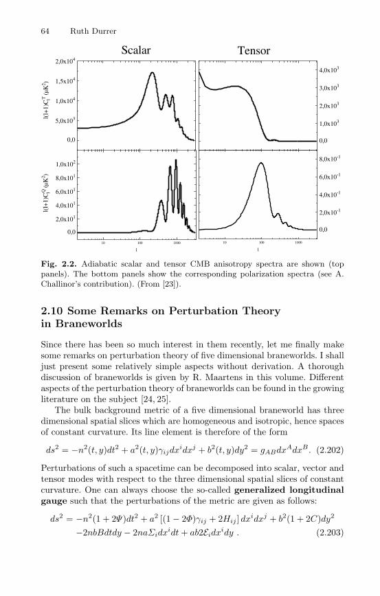
64 Ruth Durrer
10 100 1000
0,0
2,0x10⁻¹
4,0x10⁻¹
6,0x10⁻¹
8,0x10⁻¹
l
0,0
5,0x10³
1,0x10⁴
1,5x10⁴
2,0x10⁴
l(l+
1)C
lT (
µ K2 )
10 100 1000
0,0
2,0x101
4,0x101
6,0x101
8,0x101
1,0x10²
l(l+
1)C
lQ (
µ K2 )
l
0,0
1,0x10³
2,0x10³
3,0x10³
4,0x10³
TensorScalar
Fig. 2.2. Adiabatic scalar and tensor CMB anisotropy spectra are shown (toppanels). The bottom panels show the corresponding polarization spectra (see A.Challinor’s contribution). (From [23]).
2.10 Some Remarks on Perturbation Theoryin Braneworlds
Since there has been so much interest in them recently, let me finally makesome remarks on perturbation theory of five dimensional braneworlds. I shalljust present some relatively simple aspects without derivation. A thoroughdiscussion of braneworlds is given by R. Maartens in this volume. Differentaspects of the perturbation theory of braneworlds can be found in the growingliterature on the subject [24, 25].
The bulk background metric of a five dimensional braneworld has threedimensional spatial slices which are homogeneous and isotropic, hence spacesof constant curvature. Its line element is therefore of the form
ds2 = −n2(t, y)dt2 + a2(t, y)γijdxidxj + b2(t, y)dy2 = gABdx
AdxB . (2.202)
Perturbations of such a spacetime can be decomposed into scalar, vector andtensor modes with respect to the three dimensional spatial slices of constantcurvature. One can always choose the so-called generalized longitudinalgauge such that the perturbations of the metric are given as follows:
ds2 = −n2(1 + 2Ψ)dt2 + a2 [(1 − 2Φ)γij + 2Hij ] dxidxj + b2(1 + 2C)dy2
−2nbBdtdy − 2naΣidxidt+ ab2Eidx
idy . (2.203)
2 Cosmological Perturbation Theory 65
Here Σi and Ei are divergence free vector fields, vector perturbations andHij is a divergence free traceless symmetric tensor, the tensor perturbation,while Ψ,Φ,C and B are four scalar perturbations.
It can be shown that this choice determines the gauge completely. Onecan actually define gauge invariant perturbation variables which reduce tothe ones above in the generalized longitudinal gauge [25]. Writing down theperturbed Einstein equations for these variables in the most general case isquite involved. These equations can be found in [25], but I don’t want torepeat them here. I just discuss their general structure in the case of anempty bulk. It is clear that Ψ and Φ correspond to the Bardeen potentials offour dimensional cosmology, Σi is the four dimensional vector perturbationand Hij represents four dimensional gravitational waves. C and B as well asEi are new degrees of freedom which are not present in the four dimensionaltheory.
If we assume vanishing perturbations of the bulk energy momentum tensore.g. if the bulk is anti de Sitter like in the Randall Sundrum model [26]called RSII in what follows (see R. Maartens’ contribution), the perturbationequations reduce to
5(Ψ + Φ) = 0 (2.204)5Σi = 0 (2.205)
5Hij = 0 , (2.206)
and all the other perturbation variables are determined by constraint equa-tions. Here 5 is the five dimensional d’Alembertian with respect to thebackground metric (2.202). This structure of the equations is to be expected:Gravitational waves in d spacetime dimensions are a spin 2 field with respectto the group of rotations SO(d − 2) since they are massless (see e.g. [27]).For d = 5, d − 2 = 3 they therefore have 5 degrees of freedom. These cor-respond exactly to the one scalar (2.204), two vector (2.205) and two tensor(2.206) degrees of freedom with respect to the 3-dimensional slices of constantcurvature. These free massless degrees of freedom obey the wave equationsabove.
The perturbed Israel junction conditions (see R. Maartens’ contribution)then determine boundary conditions for the behaviour of the perturbationsat the brane position(s).
As an example, I write down the vector and tensor perturbation equationsand their bulk solutions for the RSII model which has only one brane. Therethe bulk is a five dimensional anti-de Sitter spacetime, and we can choosecoordinates so that the background metric has the form
ds2 =(L
y
)2 [−dt2 + δijdxidxj + dy2]
(2.207)
and
66 Ruth Durrer
5 = −∂2t + + ∂2
y − 3y∂y , (2.208)
where denotes the three dimensional spatial Laplacian. For an arbitrarymode which satisfies this wave equation we make the ansatz
φ(t,x, y) = exp(i(k · x − ωt))φ(ω,k, y) .We then obtain a Bessel differential equation for φ(ω,k, y) with general so-lution
φ = A(ω,k)(ym)2J2(my) +B(ω,k)(ym)2Y2(my) , m2 = ω2 − k2 ,
= φA + φB . (2.209)
These modes are normalizable in the sense that∫ ∞
yb
|φ|2√−gdy < ∞ .
Here yb > 0 is the brane position. The Israel junction condition for the vectorand tensor modes for RSII become
−∂yHij(y = yb) = κ25Πij(yb) (2.210)
−Σi(yb) = κ25Πi(yb) , (2.211)
where Πij respectively Πi are the tensor respectively vector contributionto the anisotropic stresses on the brane. If the latter vanish, the junctioncondition simple requires
B(ω,k) = A(ω,k)J2(myb)/Y2(myb) .
This result has been derived for the tensor mode by Randall and Sun-drum [26]. For scalar perturbations the situation is somewhat more com-plicated since there is an additional degree of freedom which is the perturbedposition of the brane, yb → yb + ε. It is rather subtle to take this brane bend-ing correctly into account. A very interesting work showing that this effectis actually most relevant to obtain the correct Newtonian limit in the RSIImodel can be found in [28].
Let us also briefly discuss the zero–mode. From the brane point of view,the modes discussed here represent waves (particles) which couple only to theenergy momentum tensor of the brane and which obey a dispersion relationω2 − k2 = m2, hence the parameter m of the solutions (2.211) is their mass.In the limit m→ 0 the solutions turn into power laws in y,
φ0(y) = Ay4 +B . (2.212)
Of these modes, for tensor and vector perturbations, the B mode is normaliz-able. For scalar perturbations the situation is more complicated. For a modeto be ‘normalizable’ we want all the perturbations to be normalizable,

2 Cosmological Perturbation Theory 67∫ ∞
yb
|φ|2√−gdy < ∞ for φ = Φ , Ψ , C and B .
But from the constraints one obtains for m = 0 C ∝ y2 which is not nor-malizable. This mode diverges logarithmically and only converges due to theoscillations of the Bessel functions if m = 0.
If all the five graviton zero–modes are normalizable, like in all compactbraneworlds, e.g. in models with two branes, the vector and scalar mode leadto three additional degrees of freedom (to the usual two four-dimensionalgraviton modes) which couple via the junction conditions to the brane energymomentum tensor and spoil the phenomenology of the model. The resultingfour dimensional gravity is not Einstein gravity but Brans–Dicke or even morecomplicated. As an example, in [29] the contribution from the scalar zero–mode (2.204) to the gravity wave emission from a binary pulsar is calculatedand shown to be in contradiction with observations. This problem is well-known from Kaluza Klein theories, it is the so called moduli problem. Theway out of it is usually to render the modes massive. There are differentsuggestions how this can be achieved for the scalar mode. One possibilityis the so called Goldberger–Wise mechanism [30] which shows that undercertain circumstances a bulk scalar field can do the job. But certainly, aphysically acceptable braneworld is defined only together with its mechanismhow to get rid of such unwanted modes (see also [31]).
The advantage of the RSII model is that the scalar gravity wave zero–mode is not normalizable in this model and therefore it does not contribute.This very promising property of the RSII model has let to its popularity. Itseems to induce the correct four dimensional Einstein gravity on the brane,in the cosmological context this property is still maintained at sufficientlylow energies.
2.11 Conclusions
In this contribution I have given an introduction to cosmological perturba-tion theory. Perturbation theory is an important tool especially to calculateCMB anisotropies and polarisation since these are very small and can bedetermined reliably within linear cosmological perturbation theory. To deter-mine the evolution of the cosmic matter density, linear perturbation theoryhas to be complemented with the theory of weakly non-linear Newtoniangravity and with N-body simulations. To finally understand the formation ofgalaxies, non-gravitational highly non-linear physics, like heating and coolingmechanisms, dissipation, nuclear reactions etc. have to be taken into account.This very difficult subject is still in its infancy.
To make progress in our understanding of braneworlds, linear perturba-tion theory can also be most helpful. We can use it to determine e.g. thepropagating modes of the gravitational field on the brane, light deflection
68 Ruth Durrer
and redshift in weak gravitational fields and the Newtonian limit. The condi-tion that linear perturbations on the brane at low energy and large distancesreduce to those resulting from Einstein gravity is non–trivial and has, to myknowledge, not yet been fully explored to limit braneworld models.
Acknowledgements
I thank the organizers for a well structured school in a most beautiful envi-ronment.
References
1. I. Newton, Letters from Sir Isaac Newton to Dr. Bentley, Letter I, 203ff quotedby A. Koyre, From the Classical World to the Infinite Universe, Harper andRow (New York 1958).
2. E. Lifshitz, JETP 10, 116 (1946).3. D. Barden and C. Thomas, An Introduction to Differential Manifolds, Imperial
College Press (2003).4. J.M. Stewart and M. Walker, Proc. R. Soc. London A341, 49 (1974).5. J. Bardeen, Phys. Rev. D22, 1882 (1980).6. H. Kodama and M. Sasaki Prog. Theor. Phys. Suppl 78, 1 (1984).7. R. Durrer, Fund. of Cosmic Physics 15, 209 (1994).8. M. Bruni, P. Dunsby and G. Ellis, Astrophys. J 395, 34 (1992).9. R. Trotta, A. Riazuelo and R. Durrer, Phys. Rev. Lett. 87, 231301 (2001).
10. M. Bucher, K. Moodley and N. Turok, Phys. Rev. D 66, 023528 (2002)11. E. Harrison, Phys. Rev. D1 2726 (1970);
Ya. B. Zel’dovich, Mont. Not. R. Astr. Soc. 160, P1 (1972).12. V. F. Mukhanov, H. A. Feldman and R. H. Brandenberger, Phys. Rept. 215,
203 (1992).13. R. Durrer, M. Kunz and A. Melchiorri, Phys. Rept. 364, 1 (2002).14. R.K. Sachs and A.M. Wolfe, Astrophys. J. 147, 73 (1967).15. M. Tegmark et al., astro-ph/0310725, (2003).16. P.J.E. Peebles, Principles of Physical Cosmology, Princeton University Press
(1993).17. G.F. Smoot et al., Astrophys. J. 396, L1 (1992).18. U. Pen, D. Spergel and N. Turok, Phys Rev. D 49, 692 (1994).19. R. Durrer and Z. Zhou, Phys. Rev. D 53, 5394 (1996).20. B. Allen et al., Phys. Rev. Lett. 79, 2624 (1997).21. R. Durrer et al., Phys. Rev. D 59, 043511 (1999)22. T. Kanazawa, M. Kawasaki, N. Sugiyama, and T. Yanagida, Prog. Theor. Phys.
100 1055 (1998).23. A. Melchiorri and N. Vittorio, in: Proceedings of the NATO Advanced Study
Institute 1996, Strasbourg, astro-ph/9610029, (1996).24. H. Kodama, A. Ishibashi, and O. Seto, Phys. Rev. D 62, 064022 (2000); D. Lan-
glois, Phys. Rev. D 62, 126012 (2000); S. Mukohyama, Phys. Rev. D 62, 084015(2000); D. Langlois, Phys. Rev. Lett. 86, 2212 (2001); H. Bridgman, K. Malik,and D. Wands, Phys. Rev. D 65, 043502 (2002); K. Koyama and J. Soda, Phys.Rev. D 65, 023514 (2002).
2 Cosmological Perturbation Theory 69
25. A. Riazuelo, F. Vernizzi, D. Steer and R. Durrer, hep-th/0205220, (2002).26. L. Randall and R. Sundrum, Phys. Rev. Lett. 83, 4690 (1999).27. S. Weinberg, The Quantum Theory of Fields, Vol I p62ff, Cambridge University
Press (1995).28. J. Garriga and T. Tanaka, Phys. Rev. Lett. 84, 2778 (2000).29. R. Durrer and P. Kocian, hep-th/0305181, (2003).30. W. Goldberger and M. Wise, Phys. Lett. B475, 275 (2000).31. J. Lesgourges and L. Sorbo, hep-th/0310007, (2003).
3 Cosmic Microwave Background Anisotropies
Anthony Challinor
Astrophysics Group, Cavendish Laboratory, Madingley Road, Cambridge,CB3 0HE, UK
Abstract. The linear anisotropies in the temperature of the cosmic microwavebackground (CMB) radiation and its polarization provide a clean picture of fluctu-ations in the universe some 370 kyr after the big bang. Simple physics connects thesefluctuations with those present in the ultra-high-energy universe, and this makesthe CMB anisotropies a powerful tool for constraining the fundamental physicsthat was responsible for the generation of structure. Late-time effects also leavetheir mark, making the CMB temperature and polarization useful probes of darkenergy and the astrophysics of reionization. In this review we discuss the simplephysics that processes primordial perturbations into the linear temperature andpolarization anisotropies. We also describe the role of the CMB in constrainingcosmological parameters, and review some of the highlights of the science extractedfrom recent observations and the implications of this for fundamental physics.
3.1 Introduction
The cosmic microwave background (CMB) radiation has played an essentialrole in shaping our current understanding of the large-scale properties of theuniverse. The discovery of this radiation in 1965 by Penzias and Wilson [1],and its subsequent interpretation as the relic radiation from a hot, densephase of the universe [2] put the hot big bang model on a firm observationalfooting. The prediction of angular variations in the temperature of the radia-tion, due to the propagation of photons through an inhomogeneous universe,followed shortly after [3], but it was not until 1992 that these were finally de-tected by the Differential Microwave Radiometers (DMR) experiment on theCosmic Background Explorer (COBE) satellite [4]. The fractional tempera-ture anisotropies are at the level of 10−5, consistent with structure formationin cold dark matter (CDM) models [5, 6], but much smaller than earlier pre-dictions for baryon-dominated universes [3, 7]. Another experiment on COBE,the Far InfraRed Absolute Spectrophotometer (FIRAS), spectacularly con-firmed the black-body spectrum of the CMB and determined the (isotropic)temperature to be 2.725 K [8, 9].
In the period since COBE, many experiments have mapped the CMBanisotropies on a range of angular scales from degrees to arcminutes (see [10]for a recent review), culminating in the first-year release of all-sky data fromthe Wilkinson Microwave Anisotropy Probe (WMAP) satellite in February
A. Challinor, Cosmic Microwave Background Anisotropies, Lect. Notes Phys. 653, 71–103 (2005)http://www.springerlink.com/ c© Springer-Verlag Berlin Heidelberg 2005

72 Anthony Challinor
2003 [11]. The observed modulation in the amplitude of the anisotropies withangular scale is fully consistent with predictions based on coherent, acous-tic oscillations [7], derived from gravitational instability of initially adiabaticdensity perturbations in a universe with nearly-flat spatial sections. The am-plitude and scale of these acoustic features has allowed many of the keycosmological parameters to be determined with unprecedented precision [12],and a strong concordance with other cosmological probes has emerged.
In this review article we describe the essential physics of the temperatureanisotropies of the CMB, and its recently-detected polarization [13], and dis-cuss how these are used to constrain cosmological models. For reviews thatare similar in spirit, but from the pre-WMAP era see e.g. [14, 15]. We beginin Sect. 3.2 with the fundamentals of CMB physics, presenting the kinetictheory of the CMB in an inhomogeneous universe, and the various physicalmechanisms that process initial fluctuations in the distribution of matter andspacetime geometry into temperature anisotropies. Sect. 3.3 discusses the ef-fect of cosmological parameters on the power spectrum of the temperatureanisotropies, and the limits to parameter determination from the CMB alone.The physics of CMB polarization is reviewed in Sect. 3.4, and the additionalinformation that polarization brings over temperature anisotropies alone isconsidered. Finally, in Sect. 3.5 we describe some of the scientific highlightsthat have emerged from recent CMB observations, including the detection ofCMB polarization, implications for inflation, and the direct signature of darkenergy through correlations between the large-scale anisotropies and tracersof the mass distribution in the local universe. Throughout, we illustrate ourdiscussion with computations based on ΛCDM cosmologies, with baryon den-sity Ωbh
2 = 0.023 and cold dark matter density Ωch2 = 0.111. For flat models
we take the dark-energy density parameter to be ΩΛ = 0.75 giving a Hubbleparameter H0 = 73 km s−1 Mpc−1. We adopt units with c = 1 throughout,and use a spacetime metric signature + − −−.
3.2 Fundamentals of CMB Physics
In this section we aim to give a reasonably self-contained review of the es-sential elements of CMB physics.
3.2.1 Thermal History and Recombination
The high temperature of the early universe maintained a low equilibriumfraction of neutral atoms, and a correspondingly high number density offree electrons. Coulomb scattering between the ions and electrons kept themin local kinetic equilibrium, and Thomson scattering of photons tended tomaintain the isotropy of the CMB in the baryon rest frame. As the universeexpanded and cooled, the dominant element hydrogen started to recombinewhen the temperature fell below ∼ 4000 K – a factor of 40 lower than might

3 Cosmic Microwave Background Anisotropies 73
be anticipated from the 13.6-eV inoization potential of hydrogen, due to thelarge ratio of the number of photons to baryons. The details of recombina-tion are complicated since the processes that give rise to net recombinationoccur too slowly to maintain chemical equilibrium between the electrons,protons and atoms during the later stages of recombination [16, 17] (see [18]for recent refinements). The most important quantity for CMB anisotropyformation is the visibility function – the probability that a photon last scat-tered as a function of time. The visibility function peaks around ∼ 370 kyrafter the big bang, and has a width ∼ 115 kyr, a small fraction of the currentage ∼ 13.5 Gyr [12]. After recombination, photons travelled mostly unim-peded through the inhomogeneous universe, imprinting fluctuations in theradiation temperature, the gravitational potentials, and the bulk velocity ofthe radiation where they last scattered, as the temperature anisotropies thatwe observe today. A small fraction of CMB photons (current results fromCMB polarization measurements [19] indicate around 20 per cent; see alsoSect. 3.5.1) underwent further scattering once the universe reionized due toto the ionizing flux from the first non-linear structures (see also R. Sander’sreview).
3.2.2 Statistics of CMB Anisotropies
The spectrum of the CMB brightness along any direction n is very nearlythermal with a temperature T (n). The temperature depends only weakly ondirection, with fluctuations ∆T (n) at the level of 10−5 of the average tem-perature T = 2.725 K. It is convenient to expand the temperature fluctuationin spherical harmonics,
∆T (n)/T =∑
lm
almYlm(n) , (3.1)
with a∗lm = (−1)mal−m since the temperature is a real field. The sum in
(3.1) runs over l ≥ 1, but the dipole (l = 1) is usually removed explicitlywhen analysing data since it depends linearly on the velocity of the observer.Multipoles at l encode spatial information with characteristic angular scale∼ π/l (see R. Durrer’s contribution).
The statistical properties of the fluctuations in a perturbed cosmology canbe expected to respect the symmetries of the background model. In the caseof Robertson–Walker models, the rotational symmetry of the backgroundensures that the multipoles alm are uncorrelated for different values of land m:
〈alma∗l′m′〉 = Clδll′δmm′ , (3.2)
which defines the power spectrum Cl. The angle brackets in this equationdenote the average over an ensemble of realisations of the fluctuations. Thesimplest models of inflation predict that the fluctuations should also be Gaus-sian at early times, and this is preserved by linear evolution of the small fluc-tuations. If Gaussian, the alms are also independent, and the power spectrum
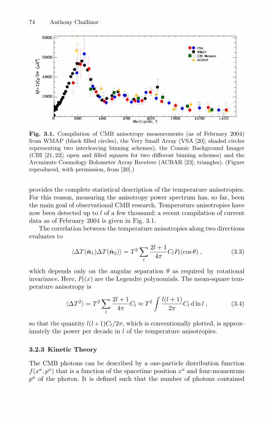
74 Anthony Challinor
Fig. 3.1. Compilation of CMB anisotropy measurements (as of February 2004)from WMAP (black filled circles), the Very Small Array (VSA [20]; shaded circlesrepresenting two interleaving binning schemes), the Cosmic Background Imager(CBI [21, 22]; open and filled squares for two different binning schemes) and theArcminute Cosmology Bolometer Array Receiver (ACBAR [23]; triangles). (Figurereproduced, with permission, from [20].)
provides the complete statistical description of the temperature anisotropies.For this reason, measuring the anisotropy power spectrum has, so far, beenthe main goal of observational CMB research. Temperature anisotropies havenow been detected up to l of a few thousand; a recent compilation of currentdata as of February 2004 is given in Fig. 3.1.
The correlation between the temperature anisotropies along two directionsevaluates to
〈∆T (n1)∆T (n2)〉 = T 2∑
l
2l + 14π
ClPl(cos θ) , (3.3)
which depends only on the angular separation θ as required by rotationalinvariance. Here, Pl(x) are the Legendre polynomials. The mean-square tem-perature anisotropy is
〈∆T 2〉 = T 2∑
l
2l + 14π
Cl ≈ T 2∫l(l + 1)
2πCl d ln l , (3.4)
so that the quantity l(l+1)Cl/2π, which is conventionally plotted, is approx-imately the power per decade in l of the temperature anisotropies.
3.2.3 Kinetic Theory
The CMB photons can be described by a one-particle distribution functionf(xa, pa) that is a function of the spacetime position xa and four-momentumpa of the photon. It is defined such that the number of photons contained
3 Cosmic Microwave Background Anisotropies 75
in a proper three-volume element d3x and with three-momentum in d3p isfd3xd3p. The phase-space volume element d3xd3p is Lorentz-invariant andis conserved along the photon path through phase space (see, e.g. [24]). Itfollows that f is also frame-invariant, and is conserved in the absence ofscattering. To calculate the anisotropies in the CMB temperature, we mustevolve the photon distribution function in the perturbed universe.
To avoid over-complicating our discussion, we shall only consider spatially-flat models here, and, for the moment, ignore the effects of polarization. For amore complete discussion, including these complications, see e.g. [25, 26]. Cur-vature mostly affects the CMB through the geometrical projection of linearscales at last scattering to angular scales on the sky today, but has a negligibleimpact on pre-recombination physics and hence much of the discussion in thissection. The subject of cosmological perturbation theory is rich in method-ology, but, for pedagogical reasons, we adopt here the most straightforwardapproach which is to work directly with the metric perturbations. This is alsothe most prevalent in the CMB literature. The (1+3)-covariant approach [27]is a well-developed alternative that is arguably more physically-transparentthan metric-based techniques. It has also been applied extensively in the con-text of CMB physics [26, 28, 29, 30, 31, 32]. The majority of our discussion willbe of scalar perturbations, where all perturbed three-tensors can be derivedfrom the spatial derivatives of scalar functions, although we discuss tensorperturbations briefly in Sect. 3.2.5.
For scalar perturbations in spatially-flat models we can choose a gaugesuch that the spacetime metric is [33]
ds2 = a2(η)[(1 + 2ψ)dη2 − (1 − 2φ)dx2] , (3.5)
where η is conformal time (related to proper time t by dt = adη), a is thescale factor in the background model and, now, x is comoving position. Thisgauge, known as the conformal Newtonian or longitudinal gauge, has theproperty that the congruence of worldlines with constant x have zero shear.The two scalar potentials φ and ψ constitute the scalar perturbation to themetric, with φ playing a similar role to the Newtonian gravitational potential.In the absence of anisotropic stress, φ and ψ are equal. We parameterise thephoton four-momentum with its energy ε/a and direction e (with e2 = 1),as seen by an observer at constant x, so that
pµ = a−2ε[1 − ψ, (1 + φ)e] . (3.6)
Free photons move on the geodesics of the perturbed metric, pµ∇µpν = 0, so
the energy and direction evolve as
dε/dη = −εdψ/dη + ε(φ+ ψ) (3.7)de/dη = −∇⊥(φ+ ψ) , (3.8)
where dots denote ∂/∂η and ∇⊥ is the three-gradient projected perpendicularto e. We see immediately that ε is conserved in the absence of perturbations,
76 Anthony Challinor
so that the energy redshifts in proportion to the scale factor in the backgroundmodel. The change in direction of the photon due to the projected gradientof the potentials in the perturbed universe gives rise to gravitational lensing(see e.g. [34] for a review).
The dominant scattering mechanism to affect CMB anisotropies is clas-sical Thomson scattering off free electrons, since around recombination theaverage photon energy is small compared to the rest mass of the electron.Furthermore, the thermal distribution of electron velocities can be ignoreddue to the low temperature. The evolution of the photon distribution functionin the presence of Thomson scattering is
dfdη
= −a(1 + ψ)neσTf +3
16πa(1 + ψ)neσT
∫f(ε, e′)[(1 + (e · e′)2] de′
− aneσTe · vbε∂f
∂ε, (3.9)
where ne is the electron (proper) number density, σT is the Thomson crosssection, and the electron peculiar velocity is vb = dx/dη. The derivative onthe left of (3.9) is along the photon path in phase space:
dfdη
=∂f
∂η+ e · ∇f + (φ− e · ∇ψ)ε
∂f
∂ε(3.10)
to first order, where we have used (3.7) and (3.8) and the fact that theanisotropies of f are first order. The first term on the right of (3.9) describesscattering out of the beam, and the second scattering into the beam. Thefinal term arises from the out-scattering of the additional dipole moment inthe distribution function seen by the electrons due to the Doppler effect. Inthe background model f is isotropic and the net scattering term vanishes, sothat f is a function of the conserved ε only: f = f(ε). Thermal equilibriumensures that f is a Planck function.
The fluctuations in the photon distribution function inherit an energydependence ε∂f/∂ε from the source terms in the Boltzmann equation (3.9).Separating out the background contribution to f , and its energy dependence,we can write
f(η,x, ε,e) = f(ε)[1 − Θ(η,x, e)d ln f/d ln ε], (3.11)
so that the CMB spectrum is Planckian but with a direction-dependent tem-perature ∆T/T = Θ. Using the Lorentz invariance of f , it is not difficult toshow that the quadrupole and higher moments of Θ are gauge-invariant. Ifwe now substitute for f in (3.9), we find the Boltzmann equation for Θ:
∂(Θ + ψ)∂η
+ e · ∇(Θ + ψ) = −aneσTΘ +3
16πaneσT
∫Θ(e′)[(1 + (e · e′)2] de′
+ aneσTe · vb + φ+ ψ . (3.12)
3 Cosmic Microwave Background Anisotropies 77
The formal solution of this equation is an integral along the line of sightn = −e,
[Θ(n) + ψ]R = e−τ [Θ(n) + ψ)]E +∫ R
E
e−τS dη , (3.13)
where R is the reception event, E is the emission event, and τ ≡ ∫ aneσT dη isthe optical depth back from R. The source term S is given by the right-handside of (3.12), but with Θ replaced by −ψ in the first term.
We gain useful insight into the physics of anisotropy formation by ap-proximating the last scattering surface as sharp (which is harmless on largeangular scales), and ignoring the quadrupole CMB anisotropy at last scat-tering. In this case (3.13) reduces to
[Θ(n) + ψ]R = Θ0|E + ψ|E − n · vb|E +∫ R
E
(ψ + φ) dη , (3.14)
where Θ0 is the isotropic part of Θ, and is proportional to the fluctuation inthe photon energy density. The various terms in this equation have a simplephysical interpretation. The temperature received along direction n is theisotropic temperature of the CMB at the last scattering event on the lineof sight, Θ0, corrected for the gravitational redshift due to the difference inpotential between E and R, and the Doppler shift e · vb|E resulting fromscattering off moving electrons. Finally, there is an additional gravitationalredshift contribution arising from evolution of the gravitational potentials [3].
Machinery for an Accurate Calculation
An accurate calculation of the CMB anisotropy on all scales where linearperturbation theory (see also R. Durrer’s contribution) is valid requires a fullnumerical solution of the Boltzmann equation. The starting point is to expandΘ(θ,x, e) in appropriate basis functions. For scalar perturbations, these arethe contraction of the (irreducible) trace-free tensor products e〈i1 . . . eil〉 (theangle brackets denoting the trace-free part) with trace-free (spatial) tensorsderived from derivatives of scalars [28, 31, 35]. Fourier expanding the scalarfunctions, we end up forming contractions between e〈i1 . . . eil〉 and k〈i1 . . . kil〉where k is the wavevector. These contractions reduce to Legendre polynomi-als of k · e, and so the normal-mode expansion of Θ for scalar perturbationstakes the form
Θ(η,x, e) =∑
l≥0
∫d3k
(2π)3/2 (−i)lΘl(η,k)Pl(k · e)eik·x . (3.15)
It is straightforward to show that the implied azimuthal symmetry aboutthe wavevector is consistent with the Boltzmann equation (3.12). Insertingthe expansion of Θ into this equation gives the Boltzmann hierarchy for themoments Θl:
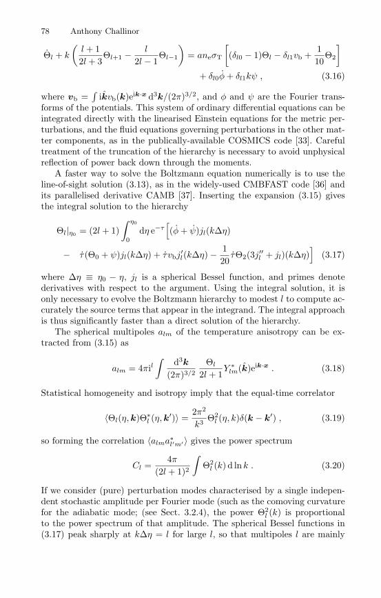
78 Anthony Challinor
Θl + k(l + 12l + 3
Θl+1 − l
2l − 1Θl−1
)= aneσT
[(δl0 − 1)Θl − δl1vb +
110
Θ2
]
+ δl0φ+ δl1kψ , (3.16)
where vb =∫
ikvb(k)eik·x d3k/(2π)3/2, and φ and ψ are the Fourier trans-forms of the potentials. This system of ordinary differential equations can beintegrated directly with the linearised Einstein equations for the metric per-turbations, and the fluid equations governing perturbations in the other mat-ter components, as in the publically-available COSMICS code [33]. Carefultreatment of the truncation of the hierarchy is necessary to avoid unphysicalreflection of power back down through the moments.
A faster way to solve the Boltzmann equation numerically is to use theline-of-sight solution (3.13), as in the widely-used CMBFAST code [36] andits parallelised derivative CAMB [37]. Inserting the expansion (3.15) givesthe integral solution to the hierarchy
Θl|η0 = (2l + 1)∫ η0
0dη e−τ
[(φ+ ψ)jl(k∆η)
− τ(Θ0 + ψ)jl(k∆η) + τ vbj′l(k∆η) − 120τΘ2(3j′′l + jl)(k∆η)
](3.17)
where ∆η ≡ η0 − η, jl is a spherical Bessel function, and primes denotederivatives with respect to the argument. Using the integral solution, it isonly necessary to evolve the Boltzmann hierarchy to modest l to compute ac-curately the source terms that appear in the integrand. The integral approachis thus significantly faster than a direct solution of the hierarchy.
The spherical multipoles alm of the temperature anisotropy can be ex-tracted from (3.15) as
alm = 4πil∫
d3k
(2π)3/2
Θl
2l + 1Y ∗
lm(k)eik·x . (3.18)
Statistical homogeneity and isotropy imply that the equal-time correlator
〈Θl(η,k)Θ∗l (η,k
′)〉 =2π2
k3 Θ2l (η, k)δ(k − k′) , (3.19)
so forming the correlation 〈alma∗l′m′〉 gives the power spectrum
Cl =4π
(2l + 1)2
∫Θ2
l (k) d ln k . (3.20)
If we consider (pure) perturbation modes characterised by a single indepen-dent stochastic amplitude per Fourier mode (such as the comoving curvaturefor the adiabatic mode; (see Sect. 3.2.4), the power Θ2
l (k) is proportionalto the power spectrum of that amplitude. The spherical Bessel functions in(3.17) peak sharply at k∆η = l for large l, so that multipoles l are mainly

3 Cosmic Microwave Background Anisotropies 79
probing spatial structure with wavenumber k ∼ l/∆η at last scattering. Theoscillatory tails of the Bessel functions mean that some power from a given kdoes also enter larger scale anisotropies. Physically, this arises from Fouriermodes that are not aligned with their wavevector perpendicular to the line ofsight. As we discuss in the next section, the tightly-coupled system of photonsand baryons undergoes acoustic oscillations prior to recombination on scalesinside the sound horizon. For the pure perturbation modes, all modes witha given wavenumber reach the maxima or minima of their oscillation at thesame time, irrespective of the direction of k, and so we expect modulationin the Cls on sub-degree scales. The first three of these acoustic peaks havenow been measured definitively; see Fig. 3.1.
3.2.4 Photon–Baryon Dynamics
Prior to recombination, the mean free path of CMB photons is ∼ 4.9 ×10⁴(Ωbh
2)−1(1+z)−2 Mpc. On comoving scales below this length the photonsand baryons behave as a tightly-coupled fluid, with the CMB almost isotropicin the baryon frame. In this limit, only the l = 0 and l = 1 moments of thedistribution function are significant.
The stress-energy tensor of the photons is given in terms of the distribu-tion function by
Tµν = a−2∫f(η,x, ε,e)pµpνεdεde , (3.21)
so that the Fourier modes of the fractional over-density of the photons areδγ = 4Θ0 and the photon (bulk) velocity vγ = −Θ1. The anisotropic stress isproportional to Θ2. In terms of these variables, the first two moment equa-tions of the Boltzmann hierarchy become
δγ − 43kvγ − 4φ = 0 (3.22)
vγ +14kδγ − 2
5kΘ2 + kψ = τ(vγ − vb) . (3.23)
Here, the derivative of the optical depth τ = −aneσT (and so is negative). Themomentum exchange between the photons and baryons due to the drag termin (3.23) gives rise to a similar term in the Euler equation for the baryons:
vb + Hvb + kψ = R−1τ(vb − vγ) , (3.24)
where we have ignored baryon pressure. The ratio of the baryon energy den-sity to the photon enthalpy is R ≡ 3ρb/4ργ and is proportional to the scalefactor a, and H ≡ a/a is the conformal Hubble parameter.
In the tightly-coupled limit |τ−1| k−1 and H−1. In this limit, we cantreat the ratios of the mean-free path to the wavelength and the Hubble timeas small perturbative parameters. Equations (3.23) and (3.24) then imply
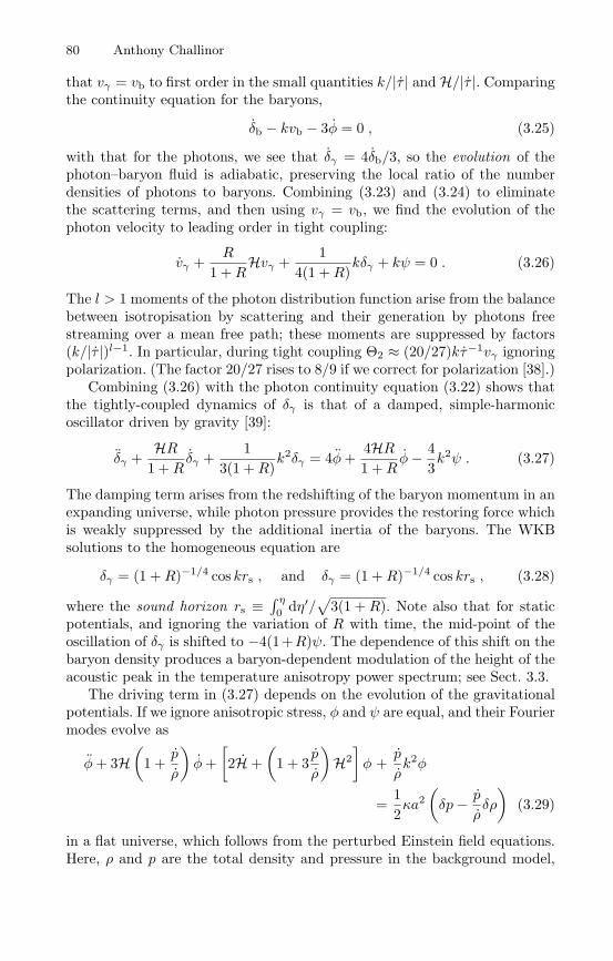
80 Anthony Challinor
that vγ = vb to first order in the small quantities k/|τ | and H/|τ |. Comparingthe continuity equation for the baryons,
δb − kvb − 3φ = 0 , (3.25)
with that for the photons, we see that δγ = 4δb/3, so the evolution of thephoton–baryon fluid is adiabatic, preserving the local ratio of the numberdensities of photons to baryons. Combining (3.23) and (3.24) to eliminatethe scattering terms, and then using vγ = vb, we find the evolution of thephoton velocity to leading order in tight coupling:
vγ +R
1 +RHvγ +
14(1 +R)
kδγ + kψ = 0 . (3.26)
The l > 1 moments of the photon distribution function arise from the balancebetween isotropisation by scattering and their generation by photons freestreaming over a mean free path; these moments are suppressed by factors(k/|τ |)l−1. In particular, during tight coupling Θ2 ≈ (20/27)kτ−1vγ ignoringpolarization. (The factor 20/27 rises to 8/9 if we correct for polarization [38].)
Combining (3.26) with the photon continuity equation (3.22) shows thatthe tightly-coupled dynamics of δγ is that of a damped, simple-harmonicoscillator driven by gravity [39]:
δγ +HR
1 +Rδγ +
13(1 +R)
k2δγ = 4φ+4HR1 +R
φ− 43k2ψ . (3.27)
The damping term arises from the redshifting of the baryon momentum in anexpanding universe, while photon pressure provides the restoring force whichis weakly suppressed by the additional inertia of the baryons. The WKBsolutions to the homogeneous equation are
δγ = (1 +R)−1/4 cos krs , and δγ = (1 +R)−1/4 cos krs , (3.28)
where the sound horizon rs ≡ ∫ η
0 dη′/√
3(1 +R). Note also that for staticpotentials, and ignoring the variation of R with time, the mid-point of theoscillation of δγ is shifted to −4(1+R)ψ. The dependence of this shift on thebaryon density produces a baryon-dependent modulation of the height of theacoustic peak in the temperature anisotropy power spectrum; see Sect. 3.3.
The driving term in (3.27) depends on the evolution of the gravitationalpotentials. If we ignore anisotropic stress, φ and ψ are equal, and their Fouriermodes evolve as
φ+ 3H(
1 +p
ρ
)φ+
[2H +
(1 + 3
p
ρ
)H2]φ +
p
ρk2φ
=12κa2(δp− p
ρδρ
)(3.29)
in a flat universe, which follows from the perturbed Einstein field equations.Here, ρ and p are the total density and pressure in the background model,

3 Cosmic Microwave Background Anisotropies 81
Fig. 3.2. Evolution of the potential φ in adiabatic and CDM-isocurvature modelsfor wavenumbers k = 0.001, 0.01 and 0.1 Mpc−1 (top to bottom respectively inmatter domination). The conformal time at matter–radiation equality ηeq and lastscattering η∗ are marked by arrows.
δρ and δp are the Fourier modes of their perturbations, and κ ≡ 8πG. Thesource term is gauge-invariant; it vanishes for mixtures of barotropic fluids[pi = pi(ρi)] with δρi/(ρi + pi) the same for all components. For adiabaticperturbations, this latter condition holds initially and is preserved on super-Hubble scales. It is also preserved in the tightly-coupled photon–baryon fluidas we saw above. For adiabatic perturbations, the potential is constant onscales larger than the sound horizon when p/ρ is constant, but decays duringtransitions in the equation of state, such as from matter to radiation dom-ination. Above the sound horizon in flat models, it can be shown that thequantity
R ≡ −φ− 2Hφ+ H2
κa2(ρ+ p)(3.30)
is conserved even through such transitions. The perturbation to the intrin-sic curvature of comoving hypersurfaces (i.e. those perpendicular to the thefour-velocity of observers who see no momentum density) is given in termsof R as 4(k2/a2)R. Using the constancy of R on large scales, the poten-tial falls by a factor of 9/10 during the transition from radiation to matterdomination. The evolution of the potential is illustrated in Fig. 3.2 in a flatΛCDM model with parameters given in Sect. 3.1. The potential oscillates in-side the sound horizon during radiation domination since the photons, whichare the dominant component at that time, undergo acoustic oscillations onsuch scales.
The behaviour of the potentials for isocurvature perturbations is quitedifferent on large scales during radiation domination [40], since the sourceterm in (3.29) is then significant. In isocurvature fluctuations, the initial per-turbations in the energy densities of the various components compensate each

82 Anthony Challinor
other in such a way that the comoving curvature R = 0. Figure 3.2 showsthe evolution of CDM-isocurvature modes, in which there is initially a largefractional perturbation in the dark matter density, with a small compensat-ing fractional perturbation in the radiation. (The full set of possibilities forregular isocurvature modes are discussed in [41].) On large scales in radiationdomination the potential grows as a, the scale factor.
Adiabatic Fluctuations
For adiabatic fluctuations, the photons are initially perturbed by δγ(0) =−2ψ(0) = 4R(0)/3, i.e. they are over-dense in potential wells, and theirvelocity vanishes vγ(0) = 0. If we consider super-Hubble scales at last scat-tering, there has been insufficient time for vγ to grow by gravitational infalland the action of pressure gradients and it remains small. The photon con-tinuity equation (3.22) then implies that δγ − 4φ remains constant, and thedecay of φ through the matter–radiation transition leaves (δγ/4 + ψ)(η∗) ≈φ(η∗)/3 = −3R(0)/5 on large scales (k < 3 × 10⁻³ Mpc−1) at last scat-tering. The combination δγ/4 + ψ = Θ0 + ψ is the dominant contributionto the large-scale temperature anisotropies produces at last scattering; see(3.14). The evolution of the photon density and velocity perturbations foradiabatic initial conditions are show in Fig. 3.3, along with the scale depen-dence of the fluctuations at last scattering. The plateau in (δγ/4 +ψ)(η∗) onlarge scales ensures that a scale-invariant spectrum of curvature perturba-tions translates into a scale-invariant spectrum of temperature anisotropies,l(l + 1)Cl = constant, for small l.
On scales below the sound horizon at last scattering, the photon–baryonfluid has had time to undergo acoustic oscillation. The form of the photon
Fig. 3.3. Evolution of the combination δγ/4+ψ (top left) and the photon velocityvγ (bottom left) which determine the temperature anisotropies produced at lastscattering (denoted by the arrow at η∗). Three modes are shown with wavenum-bers k = 0.001, 0.1 and 0.2 Mpc−1, and the initial conditions are adiabatic. Thefluctuations at the time of last scattering are shown as a function of linear scale inthe right-hand plot.
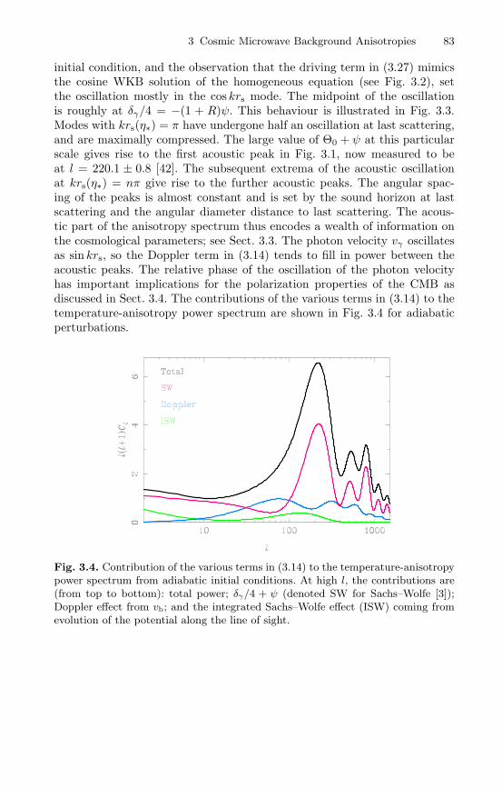
3 Cosmic Microwave Background Anisotropies 83
initial condition, and the observation that the driving term in (3.27) mimicsthe cosine WKB solution of the homogeneous equation (see Fig. 3.2), setthe oscillation mostly in the cos krs mode. The midpoint of the oscillationis roughly at δγ/4 = −(1 + R)ψ. This behaviour is illustrated in Fig. 3.3.Modes with krs(η∗) = π have undergone half an oscillation at last scattering,and are maximally compressed. The large value of Θ0 + ψ at this particularscale gives rise to the first acoustic peak in Fig. 3.1, now measured to beat l = 220.1 ± 0.8 [42]. The subsequent extrema of the acoustic oscillationat krs(η∗) = nπ give rise to the further acoustic peaks. The angular spac-ing of the peaks is almost constant and is set by the sound horizon at lastscattering and the angular diameter distance to last scattering. The acous-tic part of the anisotropy spectrum thus encodes a wealth of information onthe cosmological parameters; see Sect. 3.3. The photon velocity vγ oscillatesas sin krs, so the Doppler term in (3.14) tends to fill in power between theacoustic peaks. The relative phase of the oscillation of the photon velocityhas important implications for the polarization properties of the CMB asdiscussed in Sect. 3.4. The contributions of the various terms in (3.14) to thetemperature-anisotropy power spectrum are shown in Fig. 3.4 for adiabaticperturbations.
Fig. 3.4. Contribution of the various terms in (3.14) to the temperature-anisotropypower spectrum from adiabatic initial conditions. At high l, the contributions are(from top to bottom): total power; δγ/4 + ψ (denoted SW for Sachs–Wolfe [3]);Doppler effect from vb; and the integrated Sachs–Wolfe effect (ISW) coming fromevolution of the potential along the line of sight.
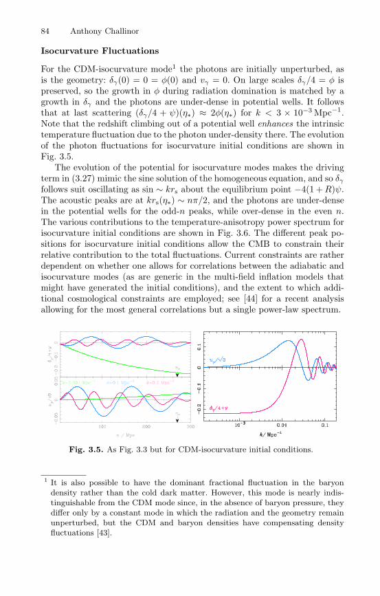
84 Anthony Challinor
Isocurvature Fluctuations
For the CDM-isocurvature mode1 the photons are initially unperturbed, asis the geometry: δγ(0) = 0 = φ(0) and vγ = 0. On large scales δγ/4 = φ ispreserved, so the growth in φ during radiation domination is matched by agrowth in δγ and the photons are under-dense in potential wells. It followsthat at last scattering (δγ/4 + ψ)(η∗) ≈ 2φ(η∗) for k < 3 × 10⁻³ Mpc−1.Note that the redshift climbing out of a potential well enhances the intrinsictemperature fluctuation due to the photon under-density there. The evolutionof the photon fluctuations for isocurvature initial conditions are shown inFig. 3.5.
The evolution of the potential for isocurvature modes makes the drivingterm in (3.27) mimic the sine solution of the homogeneous equation, and so δγfollows suit oscillating as sin ∼ krs about the equilibrium point −4(1 +R)ψ.The acoustic peaks are at krs(η∗) ∼ nπ/2, and the photons are under-densein the potential wells for the odd-n peaks, while over-dense in the even n.The various contributions to the temperature-anisotropy power spectrum forisocurvature initial conditions are shown in Fig. 3.6. The different peak po-sitions for isocurvature initial conditions allow the CMB to constrain theirrelative contribution to the total fluctuations. Current constraints are ratherdependent on whether one allows for correlations between the adiabatic andisocurvature modes (as are generic in the multi-field inflation models thatmight have generated the initial conditions), and the extent to which addi-tional cosmological constraints are employed; see [44] for a recent analysisallowing for the most general correlations but a single power-law spectrum.
Fig. 3.5. As Fig. 3.3 but for CDM-isocurvature initial conditions.
1 It is also possible to have the dominant fractional fluctuation in the baryondensity rather than the cold dark matter. However, this mode is nearly indis-tinguishable from the CDM mode since, in the absence of baryon pressure, theydiffer only by a constant mode in which the radiation and the geometry remainunperturbed, but the CDM and baryon densities have compensating densityfluctuations [43].

3 Cosmic Microwave Background Anisotropies 85
Fig. 3.6. As Fig. 3.4 but for CDM-isocurvature initial conditions. The initial spec-trum of entropy perturbations is scale-invariant.
Beyond Tight-Coupling
On small scales it is necessary to go beyond tight-coupling of the photon–baryon system since the photon diffusion length can become comparable tothe wavelength of the fluctuations. Photons that have had sufficient timeto diffuse of the order of a wavelength can leak out of over-densities, thusdamping the acoustic oscillations and generating anisotropy [45]. A roughestimate of the comoving scale below which diffusion is important is thesquare root of the geometric mean of the particle horizon (or conformal age)and the mean-free path of the photons, i.e.
√η/|τ |. Converting this to a
comoving wavenumber defines the damping scale
k−2D ∼ 0.3(Ωmh
2)−1/2(Ωbh2)−1(a/a∗)5/2 Mpc2 (3.31)
when the scale factor is a. Here, a∗ is the scale factor at last scattering, andthe expression is valid well after matter–radiation equality but well beforerecombination. The effect of diffusion is to damp the photon (and baryon)oscillations exponentially by the time of last scattering on comoving scalessmaller than ∼ 3 Mpc. The resulting damping effect on the temperature powerspectrum has now been measured by several experiments [20, 22, 23].
To describe diffusion damping more quantitatively, we consider scales thatwere already sub-Hubble during radiation domination. The gravitational po-tentials will then have been suppressed during their oscillatory phase whenthe photons (which are undergoing acoustic oscillations themselves) domi-nated the energy density, and so we can ignore gravitational effects. Fur-thermore, the dynamical timescale of the acoustic oscillations is then shortcompared to the expansion time and we can ignore the effects of expansion.In this limit, the Euler equations for the photons and the baryons can be it-erated to give the relative velocity between the photons and baryons to first

86 Anthony Challinor
order in k/|τ |:(1 +R−1)(vγ − vb) =
14kτ−1δγ . (3.32)
Using momentum conservation for the total photon–baryon system gives
vγ +Rvb +14kδγ − 2
5kΘ2 = 0 , (3.33)
which can be combined with the derivative of (3.32) to give a new Eulerequation for the photons correct to first order in tight coupling:
(1 +R)vγ ≈ −14kδγ +
R2
4(1 +R)kτ−1δγ +
1645k2τ−1vγ . (3.34)
Here, we have used Θ2 ≈ 8kτ−1vγ/9 which includes the correction due topolarization. In the limit of perfect coupling, (3.34) reduces to (3.26) onsmall scales. The continuity equation for the photons, δγ = 4kvγ/3 (+4φ),shows that the last two terms on the right of (3.34) are drag terms, and ondifferentiating gives
δγ − k2τ−1
3(1 +R)
(1615
+R2
1 +R
)δγ +
k2
3(1 +R)δγ = 0 . (3.35)
The WKB solution is
δγ ∝ e±ikrse−k2/k2D , where
1k2D
≡ 16
∫ η
0
|τ−1|1 +R
(1615
+R2
1 +R
)dη′
(3.36)is the damping scale.
The finite mean-free path of CMB photons around last scattering hasan additional effect on the temperature anisotropies. The visibility function−τeτ has a finite width ∼ 80 Mpc and so along a given line of sight photonswill be last scattered over this interval. Averaging over scattering events willtend to wash out the anisotropy from wavelengths short compared to thewidth of the visibility function. This effect is described mathematically byintegrating the oscillations in the spherical Bessel functions in (3.17) againstthe product of the visibility function and the (damped) perturbations.
Boltzmann codes such as CMBFAST [36] and CAMB [37] use the tight-coupling approximation at early times to avoid the numerical problems asso-ciated with integrating the stiff Euler equations in their original forms (3.23)and (3.24).
3.2.5 Other Features of the Temperature-AnisotropyPower Spectrum
We end this section on the fundamentals of the physics of CMB temperatureanisotropies by reviewing three additional effects that contribute to the linearanisotropies.
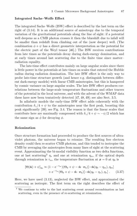
3 Cosmic Microwave Background Anisotropies 87
Integrated Sachs–Wolfe Effect
The integrated Sachs–Wolfe (ISW) effect is described by the last term on theright of (3.14). It is an additional source of anisotropy due to the temporalvariation of the gravitational potentials along the line of sight: if a potentialwell deepens as a CMB photon crosses it then the blueshift due to infall willbe smaller than redshift from climbing out of the (now deeper) well. (Thecombination φ+ ψ has a direct geometric interpretation as the potential forthe electric part of the Weyl tensor [46].) The ISW receives contributionsfrom late times as the potentials decay during dark-energy domination, andat early times around last scattering due to the finite time since matter–radiation equality.
The late-time effect contributes mainly on large angular scales since thereis little power in the potentials at late times on scales that entered the Hubbleradius during radiation domination. The late ISW effect is the only way toprobe late-time structure growth (and hence e.g. distinguish between differ-ent dark-energy models) with linear CMB anisotropies, but this is hamperedby cosmic variance on large angular scales. The late ISW effect produces cor-relations between the large-scale temperature fluctuations and other tracersof the potential in the local universe, and with the advent of the WMAP datathese have now been tentatively detected [47, 48, 49]; see also Sect. 3.5.
In adiabatic models the early-time ISW effect adds coherently with thecontribution δγ/4 + ψ to the anisotropies near the first peak, boosting thispeak significantly [39]; see Fig. 3.4. The reason is that the linear scales thatcontribute here are maximally compressed with δγ/4 + ψ ∼ −ψ/2 which hasthe same sign as φ for decaying φ.
Reionization
Once structure formation had proceeded to produce the first sources of ultra-violet photons, the universe began to reionize. The resulting free electrondensity could then re-scatter CMB photons, and this tended to isotropise theCMB by averaging the anisotropies from many lines of sight at the scatteringevent. Approximating the bi-modal visibility function as two delta functions,one at last scattering2 η∗ and one at reionization ηre, if the optical depththrough reionization is τre, the temperature fluctuation at x = 0 at η0 is
[Θ(n) + ψ]η0 ≈ (1 − e−τre)(Θ0 + ψ − n · vb)[−n(η0 − ηre), ηre]+ e−τre(Θ0 + ψ − n · vb)[−n(η0 − η∗), η∗] . (3.37)
Here, we have used (3.13), neglected the ISW effect, and approximated thescattering as isotropic. The first term on the right describes the effect of2 We continue to refer to the last scattering event around recombination as last
scattering, even in the presence of re-scattering at reionization.

88 Anthony Challinor
blending the anisotropies from different lines of sight (to give Θ0) and thegeneration of new anisotropies by re-scattering off moving electrons at reion-ization; the second term is simply the temperature anisotropy that wouldbe observed with no reionization, weighted by the fraction of photons thatdo not re-scatter. Since Θ0 + ψ at the re-scattering event is the averageof Θ0 + ψ − n′ · vb on the electron’s last scattering surface, on large scalesk(ηre −η∗) 1 it reduces to Θ0 +ψ at [−n(η0 −η∗), η∗], while on small scalesit vanishes. It follows that for scales that are super-horizon at reionization,the observed temperature anisotropy becomes
Θ(n) → Θ(n) − (1 − e−τre)n · ∆vb , (3.38)
where ∆vb is the difference between the electron velocity at the reionizationevent and the preceding last scattering event on the line of sight. On suchscales the Doppler terms do not contribute significantly and the temperatureanisotropy is unchanged. For scales that are sub-horizon at reionization,
Θ(n) → e−τreΘ(n) − (1 − e−τre)n · vb , (3.39)
where the Doppler term is evaluated at reionization. In practice, the visibilityfunction is not perfectly sharp at reionization and the integral through thefinite re-scattering distance tends to wash out the Doppler term since onlyplane waves with their wavevectors near the line of sight contribute signifi-cantly to n · vb. Figure 3.7 shows the resulting effect Cl → e−2τreCl on theanisotropy power spectrum on small scales. Recent results from WMAP [19]suggest an optical depth through reionization τre ∼ 0.17. Such early reioniza-tion cannot have been an abrupt process since the implied redshift zre ∼ 15is at odds with the detection of traces of smoothly-distributed neutral hy-drogen at z ∼ 6 via Gunn-Peterson troughs in the spectra of high-redshiftquasars [50, 51].
Tensor Modes
Tensor modes, describing gravitational waves, represent the transverse trace-free perturbations to the spatial metric:
ds2 = a2(η)[dη2 − (δij + hij)dxidxj ] , (3.40)
with hii = 0 and ∂ih
ij = 0. A convenient parameterisation of the photon
four-momentum in this case is
pµ =ε
a2
[1, ei − 1
2hi
jej
], (3.41)
where e2 = 1 and ε is a times the energy of the photon as seen by anobserver at constant x. The components of e are the projections of the photon
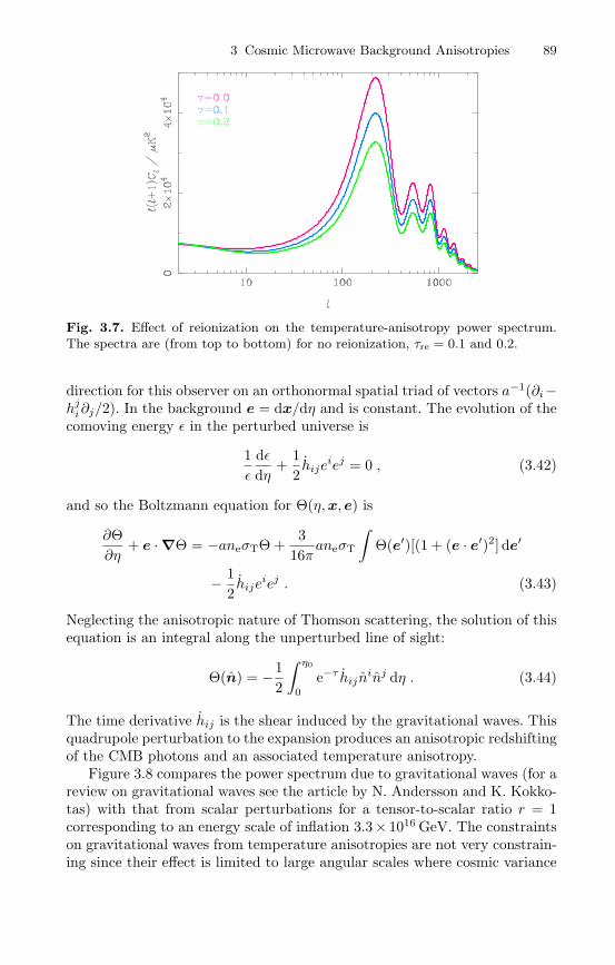
3 Cosmic Microwave Background Anisotropies 89
Fig. 3.7. Effect of reionization on the temperature-anisotropy power spectrum.The spectra are (from top to bottom) for no reionization, τre = 0.1 and 0.2.
direction for this observer on an orthonormal spatial triad of vectors a−1(∂i−hj
i∂j/2). In the background e = dx/dη and is constant. The evolution of thecomoving energy ε in the perturbed universe is
1ε
dεdη
+12hije
iej = 0 , (3.42)
and so the Boltzmann equation for Θ(η,x, e) is
∂Θ∂η
+ e · ∇Θ = −aneσTΘ +3
16πaneσT
∫Θ(e′)[(1 + (e · e′)2] de′
− 12hije
iej . (3.43)
Neglecting the anisotropic nature of Thomson scattering, the solution of thisequation is an integral along the unperturbed line of sight:
Θ(n) = −12
∫ η0
0e−τ hij n
inj dη . (3.44)
The time derivative hij is the shear induced by the gravitational waves. Thisquadrupole perturbation to the expansion produces an anisotropic redshiftingof the CMB photons and an associated temperature anisotropy.
Figure 3.8 compares the power spectrum due to gravitational waves (for areview on gravitational waves see the article by N. Andersson and K. Kokko-tas) with that from scalar perturbations for a tensor-to-scalar ratio r = 1corresponding to an energy scale of inflation 3.3 × 10¹⁶ GeV. The constraintson gravitational waves from temperature anisotropies are not very constrain-ing since their effect is limited to large angular scales where cosmic variance
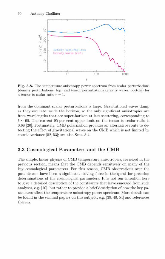
90 Anthony Challinor
Fig. 3.8. The temperature-anisotropy power spectrum from scalar perturbations(density perturbations; top) and tensor perturbations (gravity waves; bottom) fora tensor-to-scalar ratio r = 1.
from the dominant scalar perturbations is large. Gravitational waves dampas they oscillate inside the horizon, so the only significant anisotropies arefrom wavelengths that are super-horizon at last scattering, corresponding tol ∼ 60. The current 95-per cent upper limit on the tensor-to-scalar ratio is0.68 [20]. Fortunately, CMB polarization provides an alternative route to de-tecting the effect of gravitational waves on the CMB which is not limited bycosmic variance [52, 53]; see also Sect. 3.4.
3.3 Cosmological Parameters and the CMB
The simple, linear physics of CMB temperature anisotropies, reviewed in theprevious section, means that the CMB depends sensitively on many of thekey cosmological parameters. For this reason, CMB observations over thepast decade have been a significant driving force in the quest for precisiondeterminations of the cosmological parameters. It is not our intention hereto give a detailed description of the constraints that have emerged from suchanalyses, e.g. [10], but rather to provide a brief description of how the key pa-rameters affect the temperature-anisotropy power spectrum. More details canbe found in the seminal papers on this subject, e.g. [39, 40, 54] and referencestherein.
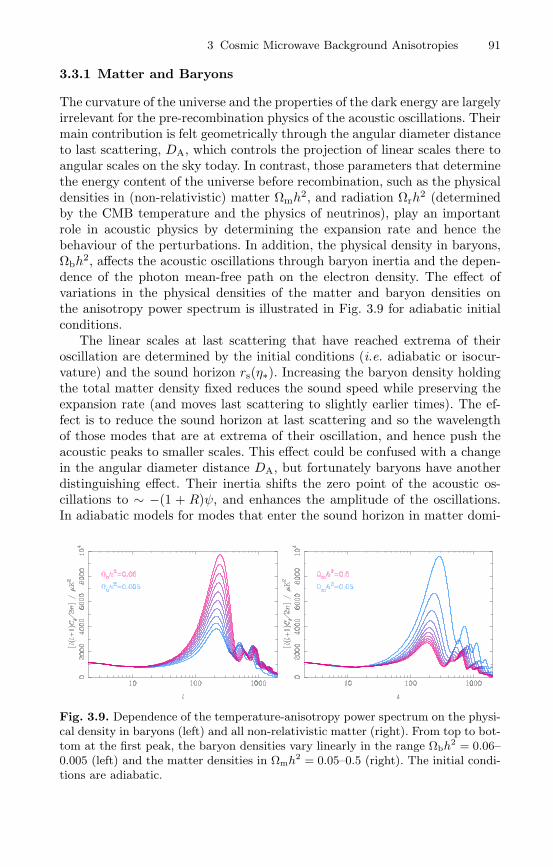
3 Cosmic Microwave Background Anisotropies 91
3.3.1 Matter and Baryons
The curvature of the universe and the properties of the dark energy are largelyirrelevant for the pre-recombination physics of the acoustic oscillations. Theirmain contribution is felt geometrically through the angular diameter distanceto last scattering, DA, which controls the projection of linear scales there toangular scales on the sky today. In contrast, those parameters that determinethe energy content of the universe before recombination, such as the physicaldensities in (non-relativistic) matter Ωmh
2, and radiation Ωrh2 (determined
by the CMB temperature and the physics of neutrinos), play an importantrole in acoustic physics by determining the expansion rate and hence thebehaviour of the perturbations. In addition, the physical density in baryons,Ωbh
2, affects the acoustic oscillations through baryon inertia and the depen-dence of the photon mean-free path on the electron density. The effect ofvariations in the physical densities of the matter and baryon densities onthe anisotropy power spectrum is illustrated in Fig. 3.9 for adiabatic initialconditions.
The linear scales at last scattering that have reached extrema of theiroscillation are determined by the initial conditions (i.e. adiabatic or isocur-vature) and the sound horizon rs(η∗). Increasing the baryon density holdingthe total matter density fixed reduces the sound speed while preserving theexpansion rate (and moves last scattering to slightly earlier times). The ef-fect is to reduce the sound horizon at last scattering and so the wavelengthof those modes that are at extrema of their oscillation, and hence push theacoustic peaks to smaller scales. This effect could be confused with a changein the angular diameter distance DA, but fortunately baryons have anotherdistinguishing effect. Their inertia shifts the zero point of the acoustic os-cillations to ∼ −(1 + R)ψ, and enhances the amplitude of the oscillations.In adiabatic models for modes that enter the sound horizon in matter domi-
Fig. 3.9. Dependence of the temperature-anisotropy power spectrum on the physi-cal density in baryons (left) and all non-relativistic matter (right). From top to bot-tom at the first peak, the baryon densities vary linearly in the range Ωbh
2 = 0.06–0.005 (left) and the matter densities in Ωmh
2 = 0.05–0.5 (right). The initial condi-tions are adiabatic.

92 Anthony Challinor
nation, δγ/4 starts out at −2ψ/3, and so the amplitude of the oscillation is−ψ(1 + 3R)/3. The combination of these two effects is to enhance the am-plitude of Θ0 + ψ at maximal compression by a factor of 1 + 6R over thatat minimal compression. The effect on the power spectrum is to enhance theamplitude of the 1st, 3rd etc. peaks for adiabatic initial conditions, and the2nd, 4th etc. for isocurvature. Current CMB data gives Ωbh
2 = 0.023±0.001for power-law ΛCDM models [12], beautifully consistent with determinationsfrom big bang nucleosynthesis. Other effects of baryons are felt in the damp-ing tail of the power spectrum since increasing the baryon density tends toinhibit diffusion giving less damping at a given scale.
The effect of increasing the physical matter density Ωmh2 at fixed Ωbh
2
is also two-fold (see Fig. 3.9): (i) a shift of the peak positions to larger scalesdue to the increase in DA; and (ii) a scale-dependent reduction in peak heightin adiabatic models. Adiabatic modes that enter the sound horizon duringradiation domination see the potentials decay as the photon density risesto reach maximal compression. This decay tends to drive the oscillation,increasing the oscillation amplitude. Raising Ωmh
2 brings matter–radiationequality to earlier times, and reduces the efficiency of the gravitational drivingeffect for the low-order peaks. Current CMB data gives Ωmh
2 = 0.13 ± 0.01for adiabatic, power-law ΛCDM models [12].
3.3.2 Curvature, Dark Energy and Degeneracies
The main effect of curvature and dark energy (see V. Sahni’s contribution) onthe linear CMB anisotropies is through the angular diameter distance and thelate-time integrated Sachs–Wolfe effect; see Fig. 3.10 for the case of adiabaticfluctuations in cosmological-constant models. The ISW contribution is limitedto large scales where cosmic variance severely limits the precision of power
Fig. 3.10. Dependence of the temperature-anisotropy power spectrum on the cur-vature ΩK (left) and cosmological constant ΩΛ (right) in adiabatic models. In bothcases, the physical densities in baryons and matter were held constant, thus pre-serving the conditions on the last scattering surface. The curvature varies (left toright) in the range -0.15–0.15 and the cosmological constant in the range 0.9–0.0.

3 Cosmic Microwave Background Anisotropies 93
Fig. 3.11. The geometric degeneracy. A scale-invariant adiabatic ΛCDM modelwith Ωbh
2 = 0.024, Ωmh2 = 0.14 and ΩΛ = 0.73 and ΩK = 0 (close to the
WMAP best-fit values [12]) produces an almost identical spectrum to a closedmodel ΩK = −0.288 with vanishing cosmological constant. However, the Hubbleconstants are very different – h = 0.72 in the flat model and 0.33 in the closedmodel – and so the latter is easily ruled out by external constraints. The shadedregion shows the 1σ cosmic variance errors ∆Cl/Cl =
√2/(2l + 1) on the power
spectrum.
spectrum estimates. There is an additional small effect due to quantisation ofthe allowed spatial modes in closed models (e.g. [55]), but this is also confinedto large scales (i.e. near the angular projection of the curvature scale). Mostof the information that the CMB encodes on curvature and dark energy isthus locked in the angular diameter distance to last scattering, DA.
With the physical densities Ωbh2 and Ωmh
2 fixed by the acoustic part ofthe anisotropy spectrum, DA can be considered a function of ΩK and thehistory of the energy density of the dark energy (often modelled throughits current density and a constant equation of state). In cosmological con-stant models DA is particularly sensitive to the curvature: the 95-per centinterval from WMAP alone (with the weak prior H0 > 50 km s−1 Mpc−1) is−0.08 < ΩK < 0.02, so the universe is close to being spatially flat. The factthat the impact of curvature and the properties of the dark energy on theCMB is mainly through a single number DA leads to a geometrical degener-acy in parameter estimation [56], as illustrated in Fig. 3.11. Fortunately, thisis easily broken by including other, complementary cosmological datasets.The constraint on curvature from WMAP improves considerably when su-pernovae measurements [57, 58], or the measurement of H0 from the HubbleSpace Telescope Key Project [59] are included. Other examples of near-perfectdegeneracies for the temperature anisotropies include the addition of gravitywaves and a reduction in the amplitude of the initial fluctuations mimicing

94 Anthony Challinor
the effect of reionization. This degeneracy is broken very effectively by thepolarization of the CMB.
3.4 CMB Polarization
The growth in the mean-free path of the CMB photons during recombinationallowed anisotropies to start to develop. Subsequent scattering of the radia-tion generated (partial) linear polarization from the quadrupole anisotropy.This linear polarization signal is expected to have an r.m.s. ∼ 5µK, and, forscalar perturbations, to peak around multipoles l ∼ 1000 corresponding to theangle subtended by the mean-free path around last scattering. The detectionof CMB polarization was first announced in 2002 by the Degree Angular ScaleInterferometer (DASI) team [13]; WMAP has also detected the polarizationindirectly through its correlation with the temperature anisotropies [19]. Adirect measurement of the polarization power from two-years of WMAP datais expected shortly. Polarization is only generated by scattering, and so is asensitive probe of conditions at recombination. In addition, large-angle polar-ization was generated by subsequent re-scattering as the universe reionized,providing a unique probe of the ionization history at high redshift.
3.4.1 Polarization Observables
Polarization is conveniently described in terms of Stokes parameters I, Q,U and V , where I is the total intensity discussed at length in the previoussection. The parameter V describes circular polarization and is expected tobe zero for the CMB since it is not generated by Thomson scattering. Theremaining parameters Q and U describe linear polarization. They are thecomponents of the trace-free, (zero-lag) correlation tensor of the electric fieldin the radiation, so that for a quasi-monochromatic plane wave propagatingalong the z direction
( 〈E2x − E2
y〉 2〈ExEy〉2〈ExEy〉 −〈E2
x − E2y〉)
=12
(Q UU −Q
), (3.45)
where the angle brackets represent an average on timescales long comparedto the period of the wave. For diffuse radiation we define the polarizationbrightness tensor Pab(n) to have components given by (3.45) for plane waveswithin a bundle around the line of sight n and around the specified frequency.The polarization tensor is transverse to the line of sight, and, since it inheritsits frequency dependence from the the quadrupole of the total intensity, hasa spectrum given by the derivative of the Planck function (see (3.11)).
The polarization tensor can be decomposed uniquely on the sphere intoan electric (or gradient) part and a magnetic (or curl) part [52, 53]:
Pab = ∇〈a∇b〉PE − εc〈a∇b〉∇cPB , (3.46)
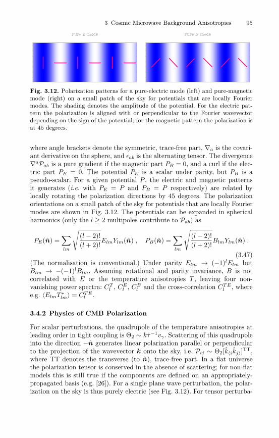
3 Cosmic Microwave Background Anisotropies 95
Fig. 3.12. Polarization patterns for a pure-electric mode (left) and pure-magneticmode (right) on a small patch of the sky for potentials that are locally Fouriermodes. The shading denotes the amplitude of the potential. For the electric pat-tern the polarization is aligned with or perpendicular to the Fourier wavevectordepending on the sign of the potential; for the magnetic pattern the polarization isat 45 degrees.
where angle brackets denote the symmetric, trace-free part, ∇a is the covari-ant derivative on the sphere, and εab is the alternating tensor. The divergence∇aPab is a pure gradient if the magnetic part PB = 0, and a curl if the elec-tric part PE = 0. The potential PE is a scalar under parity, but PB is apseudo-scalar. For a given potential P , the electric and magnetic patternsit generates (i.e. with PE = P and PB = P respectively) are related bylocally rotating the polarization directions by 45 degrees. The polarizationorientations on a small patch of the sky for potentials that are locally Fouriermodes are shown in Fig. 3.12. The potentials can be expanded in sphericalharmonics (only the l ≥ 2 multipoles contribute to Pab) as
PE(n) =∑
lm
√(l − 2)!(l + 2)!
ElmYlm(n) , PB(n) =∑
lm
√(l − 2)!(l + 2)!
BlmYlm(n) .
(3.47)(The normalisation is conventional.) Under parity Elm → (−1)lElm butBlm → −(−1)lBlm. Assuming rotational and parity invariance, B is notcorrelated with E or the temperature anisotropies T , leaving four non-vanishing power spectra: CT
l , CEl , CB
l and the cross-correlation CTEl , where
e.g. 〈ElmT∗lm〉 = CTE
l .
3.4.2 Physics of CMB Polarization
For scalar perturbations, the quadrupole of the temperature anisotropies atleading order in tight coupling is Θ2 ∼ kτ−1vγ . Scattering of this quadrupoleinto the direction −n generates linear polarization parallel or perpendicularto the projection of the wavevector k onto the sky, i.e. Pij ∼ Θ2[k〈ikj〉]TT,where TT denotes the transverse (to n), trace-free part. In a flat universethe polarization tensor is conserved in the absence of scattering; for non-flatmodels this is still true if the components are defined on an appropriately-propagated basis (e.g. [26]). For a single plane wave perturbation, the polar-ization on the sky is thus purely electric (see Fig. 3.12). For tensor perturba-
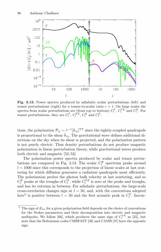
96 Anthony Challinor
Fig. 3.13. Power spectra produced by adiabatic scalar perturbations (left) andtensor perturbations (right) for a tensor-to-scalar ratio r = 1. On large scales thespectra from scalar perturbations are (from top to bottom) CT
l , CTEl and CE
l . Fortensor perturbations, they are CT
l , CTEl , CB
l and CEl .
tions, the polarization Pij ∼ τ−1[hij ]TT since the tightly-coupled quadrupoleis proportional to the shear hij . The gravitational wave defines additional di-rections on the sky when its shear is projected, and the polarization patternis not purely electric. Thus density perturbations do not produce magneticpolarization in linear perturbation theory, while gravitational waves produceboth electric and magnetic [52, 53].
The polarization power spectra produced by scalar and tensor pertur-bations are compared in Fig. 3.13. The scalar CE
l spectrum peaks aroundl ∼ 1000 since this corresponds to the projection of linear scales at last scat-tering for which diffusion generates a radiation quadrupole most efficiently.The polarization probes the photon bulk velocity at last scattering, and soCE
l peaks at the troughs of CTl , while CTE
l is zero at the peaks and troughs,and has its extrema in between. For adiabatic perturbations, the large-scalecross-correlation changes sign at l ∼ 50, and, with the conventions adoptedhere3 is positive between l = 50 and the first acoustic peak in CT
l . Isocur-
3 The sign of Elm for a given polarization field depends on the choice of conventionsfor the Stokes parameters and their decomposition into electric and magneticmultipoles. We follow [60], which produces the same sign of CTE
l as [25], butnote that the Boltzmann codes CMBFAST [36] and CAMB [37] have the oppositesign.
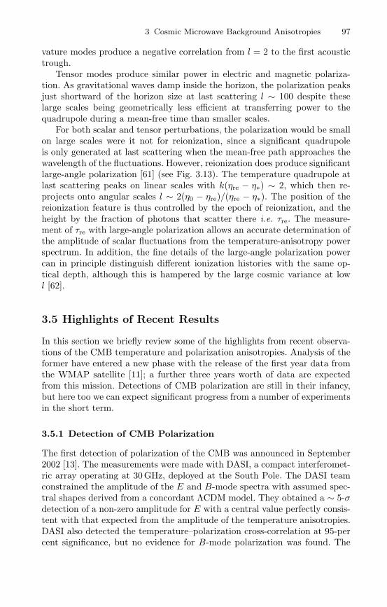
3 Cosmic Microwave Background Anisotropies 97
vature modes produce a negative correlation from l = 2 to the first acoustictrough.
Tensor modes produce similar power in electric and magnetic polariza-tion. As gravitational waves damp inside the horizon, the polarization peaksjust shortward of the horizon size at last scattering l ∼ 100 despite theselarge scales being geometrically less efficient at transferring power to thequadrupole during a mean-free time than smaller scales.
For both scalar and tensor perturbations, the polarization would be smallon large scales were it not for reionization, since a significant quadrupoleis only generated at last scattering when the mean-free path approaches thewavelength of the fluctuations. However, reionization does produce significantlarge-angle polarization [61] (see Fig. 3.13). The temperature quadrupole atlast scattering peaks on linear scales with k(ηre − η∗) ∼ 2, which then re-projects onto angular scales l ∼ 2(η0 − ηre)/(ηre − η∗). The position of thereionization feature is thus controlled by the epoch of reionization, and theheight by the fraction of photons that scatter there i.e. τre. The measure-ment of τre with large-angle polarization allows an accurate determination ofthe amplitude of scalar fluctuations from the temperature-anisotropy powerspectrum. In addition, the fine details of the large-angle polarization powercan in principle distinguish different ionization histories with the same op-tical depth, although this is hampered by the large cosmic variance at lowl [62].
3.5 Highlights of Recent Results
In this section we briefly review some of the highlights from recent observa-tions of the CMB temperature and polarization anisotropies. Analysis of theformer have entered a new phase with the release of the first year data fromthe WMAP satellite [11]; a further three years worth of data are expectedfrom this mission. Detections of CMB polarization are still in their infancy,but here too we can expect significant progress from a number of experimentsin the short term.
3.5.1 Detection of CMB Polarization
The first detection of polarization of the CMB was announced in September2002 [13]. The measurements were made with DASI, a compact interferomet-ric array operating at 30 GHz, deployed at the South Pole. The DASI teamconstrained the amplitude of the E and B-mode spectra with assumed spec-tral shapes derived from a concordant ΛCDM model. They obtained a ∼ 5-σdetection of a non-zero amplitude for E with a central value perfectly consis-tent with that expected from the amplitude of the temperature anisotropies.DASI also detected the temperature–polarization cross-correlation at 95-percent significance, but no evidence for B-mode polarization was found. The
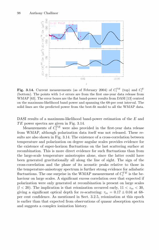
98 Anthony Challinor
Fig. 3.14. Current measurements (as of February 2004) of CTEl (top) and CE
l
(bottom). The points with 1-σ errors are from the first one-year data release fromWMAP [63]. The error boxes are the flat band-power results from DASI [13] centredon the maximum-likelihood band power and spanning the 68-per cent interval. Thesolid lines are the predicted power from the best-fit model to all the WMAP data.
DASI results of a maximum-likelihood band-power estimation of the E andTE power spectra are given in Fig. 3.14.
Measurements of CTEl were also provided in the first-year data release
from WMAP, although polarization data itself was not released. These re-sults are also shown in Fig. 3.14. The existence of a cross-correlation betweentemperature and polarization on degree angular scales provides evidence forthe existence of super-horizon fluctuations on the last scattering surface atrecombination. This is more direct evidence for such fluctuations than fromthe large-scale temperature anisotropies alone, since the latter could havebeen generated gravitationally all along the line of sight. The sign of thecross-correlation and the phase of its acoustic peaks relative to those inthe temperature-anisotropy spectrum is further strong evidence for adiabaticfluctuations. The one surprise in the WMAP measurement of CTE
l is the be-haviour on large scales. A significant excess correlation over that expected ifpolarization were only generated at recombination is present on large scales(l < 20). The implication is that reionization occurred early, 11 < zre < 30,giving a significant optical depth for re-scattering: τre = 0.17 ± 0.04 at 68-per cent confidence. As mentioned in Sect. 3.2.5, reionization at this epochis earlier than that expected from observations of quasar absorption spectraand suggests a complex ionization history.

3 Cosmic Microwave Background Anisotropies 99
3.5.2 Implications of Recent Results for Inflation
The generic predictions from simple inflation models are that: (i) the uni-verse should be (very nearly) spatially flat; (ii) there should be a nearlyscale-invariant spectrum of Gaussian, adiabatic density perturbations givingapparently-super-horizon fluctuations on the last scattering surface; and (iii)there should be a stochastic background of gravitational waves with a nearlyscale-invariant (but necessarily not blue) spectrum. The amplitude of thelatter is a direct measure of the Hubble rate during inflation, and hence, inslow-roll models, the energy scale of inflation.
As discussed in Sect. 3.3.2, the measured positions of the acoustic peaksconstrains the universe to be close to flat. The constraint improves furtherwith the inclusion of other cosmological data. There is no evidence for isocur-vature modes in the CMB, although the current constraints are rather weakif general, correlated modes are allowed in the analysis [44]. Several of thecosmological parameters for the isocurvature models most favoured by CMBdata are violently at odds with other probes, most notably the baryon den-sity which is pushed well above the value inferred from the abundances ofthe light-elements. There is also no evidence for primordial non-Gaussianityin the CMB (see e.g. [64])4.
Within flat ΛCDM models with a power-law spectrum of curvature fluc-tuations, the spectral index is constrained by the CMB to be close to scaleinvariant [12], although the inclusion of the latest data from small-scale ex-periments, such as CBI [70] and VSA [71], tends to pull the best fit fromWMAP towards redder power-law spectra: e.g. ns = 0.97+0.06
−0.03 at 68-per centconfidence combining WMAP and VSA [71]. Slow-roll inflation predicts thatthe fluctuation spectrum should be close to a power law, with a run in thespectral index that is second order in slow roll: dns/d ln k ∼ (ns − 1)2. TheWMAP team reported weak evidence for a running spectral index by includ-ing small-scale data from galaxy redshift surveys and the Lyman-α forest, butmodelling uncertainties in the latter have led many to question the reliabilityof this result (e.g. [72]). New data from CBI and VSA now provide indepen-dent evidence for running in flat ΛCDM models at the 2-σ level from the CMBalone. This reflects the tension between the spectral index favoured by thelow-l CMB data (which is anomalously low for l < 10, favouring bluer spec-tra) and the high-l data from the interferometers. The evidence for runningis weakened considerably with the inclusion of external priors from large-scale structure data. The best-fit values for the run in ns obtained with theCMB alone are uncomfortably large for slow-roll inflation models, and givelow power on small scales that is difficult to reconcile with the early reioniza-tion implied by the WMAP polarization data. However, a recent analysis [73]4 The WMAP data does appear to harbour some statistically-significant depar-
tures from rotational invariance [65, 66, 67, 68, 69]. The origin of these effects,i.e. primordial or systematic due to instrument effects or imperfect foregroundsubtraction, is as yet unclear.
100 Anthony Challinor
argues that the evidence for running depends crucially on the techniques em-ployed to estimate the low-l power from WMAP data, and that the runningis strongly suppressed if exact likelihood techniques are adopted. A definitiveanswer on whether departures from power-law spectra are significant mustprobably await further data on both large and small scales.
The final prediction of slow-roll inflation – the generation of nearly scale-invariant background of gravitational waves – is yet to be verified. The currentlimits on the tensor-to-scalar ratio are only weak: [71] report r < 0.68 at95-per cent confidence from all CMB data in general, non-flat, adiabaticΛCDM models. Despite this, observations are beginning to place interestingconstraints on specific models of inflation in the r–ns plane [74, 75]. Already,large-field models with power-law potentials steeper than V ∝ φ6 are ruledout due to their red scalar spectra and comparatively large tensor-to-scalarratio. Future programmes targeting B-mode polarization may ultimately beable to detect gravitational waves down to an inflationary energy scale of afew × 1015 GeV. Such observations will sharpen constraints in the r–ns planeconsiderably, and should allow fine selection amongst the many proposedmodels of inflation.
3.5.3 Detection of Late-Time Integrated Sachs–Wolfe Effect
The late-time ISW effect arises from the decay of the gravitational po-tentials once the universe becomes dark-energy dominated, and so shouldproduce large-angle (positive) correlations between the CMB temperatureanisotropies and other tracers of the potential in the local universe. With theadvent of the WMAP data, a number of groups have reported the detectionof such a correlation. In [47], WMAP data was cross-correlated with dataon the hard X-ray background (which is dominated by emission from activegalaxies) from the HEAO-1 satellite, and the number density of radio sourcesfrom the NVSS catalogue. In each case a positive correlation was detectedat significance 3σ and 2.5σ respectively. The correlation with NVSS has alsobeen carried out independently by the WMAP team [48], who also note thatthe observed positive correlation can be used to rule out the closed, Λ = 0model that is a good fit to the CMB data in isolation (see Fig. 3.11). Severalgroups have now also detected the cross-correlation on large scales betweenthe CMB and optical galaxy surveys, e.g. [49].
3.6 Conclusions
The linear anisotropies of the cosmic microwave background have been stud-ied theoretically for over three decades. The physics, which is now well un-derstood, employs linearised radiative transfer, general relativity, and hydro-dynamics to describe the propagation of CMB photons and the evolution ofthe fluid constituents in a perturbed Friedmann-Robertson-Walker universe.
3 Cosmic Microwave Background Anisotropies 101
A number of bold predictions have emerged from this theoretical activity,most notably the existence of acoustic peaks in the anisotropy power spec-trum due to oscillations in the photon–baryon plasma prior to recombination.Observers have risen to the challenge of verifying these predictions, and theirdetection is proceeding at a staggering rate. The large-scale Sachs–Wolfe ef-fect, acoustic peak structure, damping tail, late-time integrated Sachs–Wolfeeffect, polarization and reionization signature have all been detected, and thefirst three have been measured in considerable detail. Already, the size andscale of these effects is allowing cosmological models to be constrained withunprecedented precision. The results are beautifully consistent with almost-scale-invariant adiabatic initial conditions evolving passively in a spatiallyflat, ΛCDM universe.
Much work still remains to be done to exploit fully the information con-tained in the CMB anisotropies. The Planck satellite, due for launch in 2007,should provide definitive mapping of the linear CMB anisotropies, and acosmic-variance limited measurement of the power spectrum up to multi-poles l ∼ 2000. This dataset will be invaluable in assessing many of the issueshinted at in the first-year release of WMAP data, such as the apparent lack ofpower on large scales and possible violations of rotational (statistical) invari-ance. Prior to Planck, a number of ground-based programmes should shedfurther light on the issue of whether departures from a power-law primordialspectrum are required on cosmological scales, and the implications of thisfor slow-roll inflation. In addition, these small-scale observations will start toexplore the rich science of secondary anisotropies, due to e.g. scattering inhot clusters [76] or bulk flows modulated by variations in the electron densityin the reionized universe [77, 78], and the weak lensing effect of large-scalestructure [79].
Detections of CMB polarization are in their infancy, but we can expectrapid progress on this front too. Accurate measurements of the power spectraof E-mode polarization, and its correlation with the temperature anisotropies,can be expected from a number of ground and balloon-borne experiments, aswell as from Planck. The ultimate goal for CMB polarimetry is to detect theB-mode signal predicted from gravitational waves. This would give a directmeasure of the energy scale of inflation, and, when combined with measure-ments of the spectrum density perturbations, place tight constraints on thedynamics of inflation. Plans are already being made for a new generationof polarimeters with the large numbers of detectors and exquisite control ofinstrument systematics needed to detect the gravity-wave signal if the energyscale of inflation is around 1016 GeV. Ultimately, confusion due to imperfectsubtraction of astrophysical foregrounds and the effects of weak lensing onthe polarization limit will limit the energy scales that we can probe withCMB polarization; see [80] and references therein.

102 Anthony Challinor
Acknowledgments
The author acknowledges a Royal Society University Research Fellowship.
References
1. A.A. Penzias, R.W. Wilson, Astrophys. J. 142, 419 (1965).2. R.H. Dicke et al, Astrophys. J. 142, 414 (1965).3. R.K. Sachs, A.M. Wolfe, Astrophys. J. 147, 73 (1967).4. G.F. Smoot et al, Astrophys. J. Lett. 396, 1 (1992).5. P.J.E. Peebles, Astrophys. J. Lett. 263, 1 (1982).6. J.R. Bond, G. Efstathiou, Astrophys. J. Lett. 285, 45 (1984).7. P.J.E. Peebles J.T. Yu, Astrophys. J. 162, 815 (1970).8. J.C. Mather et al, Astrophys. J. 420, 439 (1994).9. J.C. Mather et al, Astrophys. J. 512, 511 (1999).
10. J.R. Bond, C.R. Contaldi, D. Pogosyan, Phil. Trans. Roy. Soc. Lond. A 361,2435 (2003).
11. C.L. Bennett et al, Astrophys. J. Suppl. 148, 1 (2003).12. D.N. Spergel et al, Astrophys. J. Suppl. 148, 175 (2003).13. J.M. Kovac et al, Nature 420, 772 (2002).14. W. Hu, S. Dodelson, Ann. Rev. Astron. Astrophys. 40, 171 (2002).15. W. Hu, Ann. Phys. 303, 203 (2003).16. P.J.E. Peebles, Astrophys. J. 153, 1 (1968).17. Y.B. Zeldovich, V.G. Kurt, R.A. Syunyaev, Journal of Experimental and
Theoretical Physics 28, 146 (1969).18. S. Seager, D.D. Sasselov, D. Scott, Astrophys. J. Suppl. 128, 407 (2000).19. A. Kogut et al, Astrophys. J. Suppl. 148, 161 (2003).20. C. Dickinson et al, preprint astro-ph/0402498, (2004).21. B.S. Mason et al, Astrophys. J. 591, 540 (2003).22. T.J. Pearson et al, Astrophys. J. 591, 556 (2003).23. C.L. Kuo et al, Astrophys. J. 600, 32 (2004).24. C.W. Misner, K.S. Thorne, J.A. Wheeler, Gravitation, (W. H. Freeman and
Company, San Francisco 1973) pp 583–590.25. W. Hu et al, Phys. Rev. D 57, 3290 (1998).26. A. Challinor, Phys. Rev. D 62, 043004 (2000).27. G.F.R. Ellis, J. Hwang, M. Bruni, Phys. Rev. D 40, 1819 (1989).28. A. Challinor, A. Lasenby, Astrophys. J. 513, 1 (1999).29. A. Challinor, Class. Quantum Grav. 17, 871 (2000).30. R. Maartens, T. Gebbie, G.F.R. Ellis, Phys. Rev. D 59, 083506 (1999).31. T. Gebbie, G.F.R. Ellis, Ann. Phys. 282, 285 (2000).32. T. Gebbie, P.K.S. Dunsby, G.F.R. Ellis, Ann. Phys. 282, 321 (2000).33. C. Ma, E. Bertschinger, Astrophys. J. 455, 7 (1995)34. M. Bartelmann, P. Schneider: Phys. Rep. 340, 291 (2001).35. M.L. Wilson, Astrophys. J. 273, 2 (1983).36. U. Seljak, M. Zaldarriaga, Astrophys. J. 469, 437 (1996).37. A. Lewis, A. Challinor, A. Lasenby, Astrophys. J. 538, 473 (2000).38. N. Kaiser, Mon. Not. R. Astron. Soc. 202, 1169 (1983).39. W. Hu, N. Sugiyama, Astrophys. J. 444, 489 (1995).

3 Cosmic Microwave Background Anisotropies 103
40. W. Hu, N. Sugiyama, Phys. Rev. D 51, 2599 (1995).41. M. Bucher, K. Moodley, N. Turok, Phys. Rev. D 62, 083508 (2000).42. L. Page et al, Astrophys. J. Suppl. 148, 233 (2003).43. C. Gordon, A. Lewis, Phys. Rev. D 67, 123513 (2003).44. M. Bucher et al, preprint astro-ph/0401417, (2004).45. J. Silk, Astrophys. J. 151, 459 (1968).46. J.M. Stewart, Class. Quantum Grav. 7, 1169 (1990).47. S. Boughn, R. Crittenden, Nature 427, 45 (2004).48. M.R. Nolta et al, preprint astro-ph/0305097, (2003).49. P. Fosalba, E. Gaztanaga and F.J. Castander, Astrophys. J. Lett. 597, 89
(2003).50. R.H. Becker et al, Astron. J. 122, 2850 (2001).51. S.G. Djorgovski et al, Astrophys. J. Lett. 560, 5 (2001).52. U. Seljak, M. Zaldarriaga, Phys. Rev. Lett. 78, 2054 (1997).53. M. Kamionkowski, A. Kosowsky, A. Stebbins, Phys. Rev. Lett. 78, 2058
(1997).54. J.R. Bond et al, Phys. Rev. Lett. 72, 13 (1994).55. L.F. Abbott, R.K. Schaefer, Astrophys. J. 308, 546 (1986).56. G. Efstathiou, J.R. Bond, Mon. Not. R. Astron. Soc. 304, 75 (1999).57. A.G. Riess et al, Astron. J. 116, 1009 (1998).58. S. Perlmutter et al, Astrophys. J. 517, 565 (1999).59. W.L. Freedman et al, Astrophys. J. 553, 47 (2001).60. A. Lewis, A. Challinor, N. Turok, Phys. Rev. D 65, 023505 (2002).61. M. Zaldarriaga, Phys. Rev. D 55, 1822 (1997).62. G. Holder et al, Astrophys. J. 595, 13 (2003).63. G. Hinshaw et al, Astrophys. J. Suppl. 148, 135 (2003).64. E. Komatsu et al, Astrophys. J. Suppl. 148, 119 (2003).65. A. de Oliveria-Costa et al, preprint astro-ph/0307282, (2003).66. P. Vielva et al, preprint astro-ph/0310273, (2003).67. C.J. Copi, D. Huterer, G.D. Starkman, preprint astro-ph/0310511, (2003).68. H.K. Erikse et al, preprint astro-ph/0401276, (2004).69. F.K. Hansen et al, preprint astro-ph/0402396, 2004.70. A.C.S. Readhead et al, preprint astro-ph/0402359, (2004).71. R. Rebolo et al, preprint astro-ph/0402466, (2004).72. U. Seljak, P. McDonald, A. Makarov, Mon. Not. R. Astron. Soc. 342, L79
(2003).73. A. Slosar, U. Seljak, A. Makarov, preprint astro-ph/0403073, (2004).74. S.M. Leach, A.R. Liddle, Mon. Not. R. Astron. Soc. 341, 1151 (2003).75. M. Tegmark et al, preprint astro-ph/0310723, (2003).76. R.A. Sunyaev, Y.B. Zeldovich, Comm. Astrophys. Space Phys. 4, 173 (1972).77. R.A. Sunyaev, Y.B. Zeldovich, Mon. Not. R. Astron. Soc. 190, 413 (1980).78. J.P. Ostriker, E.T. Vishniac, Astrophys. J. Lett. 306, 51 (1986).79. A. Blanchard, J. Schneider, Astron. Astrophys. 184, 1 (1987).80. C.M. Hirata, U. Seljak, Phys. Rev. D 68, 083002 (2003).
4 Observational Cosmology
Robert H. Sanders
Kapteyn Astronomical Institute, Groningen, The Netherlands
Abstract. I discuss the classical cosmological tests, i.e., angular size-redshift, flux-redshift, and galaxy number counts, in the light of the cosmology prescribed by theinterpretation of the CMB anisotropies. The discussion is somewhat of a primerfor physicists, with emphasis upon the possible systematic uncertainties in the ob-servations and their interpretation. Given the curious composition of the Universeinherent in the emerging cosmological model, I stress the value of searching forinconsistencies rather than concordance, and suggest that the prevailing mood oftriumphalism in cosmology is premature.
4.1 Introduction
The traditional cosmological tests appear to have been overshadowed by ob-servations of the anisotropies in the cosmic microwave background (CMB).We are told that these observations accurately measure the geometry of theUniverse, its composition, its present expansion rate, and the nature and formof the primordial fluctuations [1]. The resulting values for these basic param-eters are very similar to those deduced earlier from a variety of observations,the so-called “concordance model”, with about 30% of the closure density ofthe Universe comprised of matter (mostly a pressureless, non-baryonic darkmatter), the remainder being in negative pressure dark energy [2]. Given thecertainty and precision of these assertions, any current discussion of observa-tional cosmology must begin with the question: Is there any room for doubt?Why should we bother with lower precision cosmological tests when we knowall of the answers anyway?
While the interpretation of the CMB anisotropies has emerged as thesingle most important cosmological tool, we must bear in mind that the con-clusions drawn do rest upon a number of assumptions, and the results arenot altogether as robust as we are, at times, led to believe. One such as-sumption, for example, is that of adiabatic initial fluctuations, that is 100%adiabatic. A small admixture of correlated isocurvature fluctuations, an as-pect of braneworld scenarios [3], can affect peak amplitudes and thus, thederived cosmological parameters. A more fundamental assumption is that ofthe validity of traditional Friedmann-Robertson-Walker (FRW) cosmology inthe post-decoupling universe. Is the expansion of the universe described bythe Friedmann equation? Even minimal changes to the right-hand-side, such
R.H. Sanders, Observational Cosmology, Lect. Notes Phys. 653, 105–137 (2005)http://www.springerlink.com/ c© Springer-Verlag Berlin Heidelberg 2005

106 Robert H. Sanders
as the equation of state of the dark energy component, can alter the angularsize distance to the last scattering surface at z=1000 and the luminosity dis-tance to distant supernovae. But even more drastic changes to the Friedmannequation, resulting from modified gravitational physics, have been proposedin attempts to remove the unattractive dark energy [4, 5].
Such suggestions reflect a general unease with the concordance model, amodel that presents us with a universe that is strange in its composition. Themost abundant form of matter consists of, as yet, undetected non-baryonicparticles originally postulated to solve the problems of structure formationand of the missing mass in bound gravitational systems such as galaxies andclusters of galaxies. In this second respect, it is fair to say that it has failed or,to be generous, not yet succeeded, because the predicted density distributionof dark halos which emerge from cosmic N-body [6] simulations appears tobe inconsistent with observations of spiral galaxies [7] or with strong lensingin clusters of galaxies [8].
Even more mysterious is the “dark energy”, the pervasive homogeneousfluid with a negative pressure which may be identified with the cosmologicalconstant, the zero-point energy density of the vacuum. The problem of thisunnaturally low energy density, 10−122 in Planck units, is well-known, asis the cosmic coincidence problem: why are we observing the Universe at atime when the cosmological constant has, fairly recently, become dynamicallyimportant [9]? To put it another way, why are the energy densities of matterand dark energy so comparable at the present epoch? This is strange becausethe density of matter dilutes with the expanding volume of the Universewhile the vacuum energy density does not. It is this problem which has led tothe proposal of dynamic dark energy, quintessence (a dark energy, possiblyassociated with a light scalar field), with an energy density that evolves withcosmic time possibly tracking the matter energy density [10, 11]. Here thedifficulty is that the field would generally be expected to have additionalobservational consequences, such as violations of the equivalence principle atsome level, possibly detectable in fifth force experiments [9].
For these reasons, it is even more important to pursue cosmological teststhat are independent of the CMB, because one might expect new physicsto appear as observations inconsistent with the concordance model. In thissense, discord is more interesting than concord; to take a Hegelian point ofview– ideas progress through dialectic, not through concordance. It is withthis in mind that I will review observational cosmology with emphasis uponCMB-independent tests.
Below I argue that the evolution of the early, pre-recombination universeis well-understood and tightly constrained by considerations of primordialnucleosynthesis. If one wishes to modify general relativity to give deviationsfrom Friedmann expansion, then such modifications are strongly constrainedat early times, at energies on the order of 1 MeV. However, cosmologicalevolution is much less constrained in the post-recombination universe wherethere is room for deviation from standard Friedmann cosmology and where

4 Observational Cosmology 107
the more classical tests are relevant. I will discuss three of these classical tests:the angular size distance test where I am obliged to refer to its powerfulmodern application with respect to the CMB anisotropies; the luminositydistance test and its application to observations of distant supernovae; andthe incremental volume test as revealed by faint galaxy number counts.
These classical tests yield results that are consistent, to lower precision,with the parameters deduced from the CMB. While one can make minimalchanges to standard cosmology, to the equation of state of the dark energyfor example, which yield different cosmological parameters, there is no com-pelling observational reason to do so. It remains the peculiar compositionand the extraordinary coincidences embodied by the concordance model thatcall for deeper insight. Such motivations for questioning a paradigm are notunprecedented; similar worries led to the inflationary scenario which, unques-tionably, has had the dominant impact on cosmological thought in the past25 years and which has found phenomenological support in the recent CMBobservations.
I am not going to discuss tests, such as the form of the luminous matterpower spectrum [12] or the amplitude of the present mass fluctuations [13],that are based upon the standard model for structure formation. I do notmean to imply that such such tests are unimportant; it is only that I restrictmyself here to the classical tests because these address more directly theissues of the global curvature and expansion history of the Universe.
I am also going to refrain, in so far as possible, from discussion of theory ofnew gravitational physics or of any other sort. The theoretical issues presentedby dark matter that can only be detected gravitationally or by an absurdlysmall but non-zero cosmological constant are essentially not problems forthe interpretive astronomer. The primary task is to realistically access thereliability of conclusions drawn from the observations, and that is what Iintend to do.
4.2 Astronomy Made Simple (for Physicists)
I think that it is fair to assume that most of you are physicists, so I beginby defining some of the units and terminology used by astronomers. I do thisbecause much of this terminology is arcane for those not in the field.
First of all there is the peculiar logarithmic scale of flux magnitudes,whereby a factor of 100 in flux is divided into five equal logarithmic intervals.The system is ancient and has its origin in the logarithmic response of thehuman eye. The ratio of the flux of two objects is then given by a differencein magnitudes, i.e.,
m2 −m1 = −2.5 log(F2/F1) (4.1)
where, one will notice, smaller magnitude means larger flux. The zero-pointof this logarithmic scale is set by some standard star such as Vega. Because
108 Robert H. Sanders
this is related to the flux, and not the luminosity of an object, it is called the“apparent” magnitude. Distant galaxies have apparent magnitudes, in visiblelight, of greater than 20, and the galaxies in the Hubble Deep Field, go downto magnitudes of 30. The magnitude is typically measured over a specifiedwavelength range or color band, such as blue (B), visual (V), or infrared (K),and these are designated mB , mV , and mK , or sometimes just B,V, and K.This is made more confusing by the fact that there are several competingphotometric systems (or sets of filters) and conversion between them is notalways simple.
With a particular photometric system one can measure the color of anastronomical object, expressed as difference in magnitudes in two bands, orcolor index; e.g.,
B − V = 2.5 log(FV /FB) . (4.2)
Here a larger B-V color index means that an object is relatively redder; asmaller B-V that the object is bluer. Unlike the apparent magnitude, this is anintrinsic property of the object. Or rather, it is intrinsic once the astronomercorrects the magnitudes in the various bands to the zero-redshift (z = 0)frame. This is called the “K-correction” and requires a knowledge of theintrinsic spectral energy distribution (SED) of the source, which could be agalaxy or a distant supernova.
The luminosity of an object is also an intrinsic property and is usuallyexpressed by astronomers as an “absolute” magnitude. This is the apparentmagnitude an object would have if it were placed at a standard distance,taken to be 10 parsecs, i.e., 3 × 10¹⁷ m (more on parsecs below). Becausethis distance is small by extragalactic standards the absolute magnitudes ofgalaxies turn out to be rather large negative numbers: MG ≈ -18 to -21.The luminosity of a galaxy LG in units of the solar luminosity L can bedetermined from the relation
MG −M = −2.5 log(LG/L) , (4.3)
where the absolute magnitude of the sun (in the V band) is 5.5. The lumi-nosities of galaxies typically range from 108 to 1011 L. The peak absolutemagnitude of a type I supernova (SNIa) is about -19.5, or comparable to anentire galaxy. This is one reason why these objects are such ideal extragalacticdistance probes.
The unit of distance used by astronomers is also archaic: the parsec whichis about 3× 10¹⁶ m or about 3 light years. This is the distance to a star withan semi-annual parallax of 1 arc second and is not a bad unit when one isdiscussing the very local region of the galaxy. Our galaxy has a diameterbetween 10 to 20 kiloparsecs, so the kiloparsec is an appropriate unit whendiscussing galactic structure. The appropriate unit of extragalactic distance,however, is the “megaparsec” or Mpc, with nearby galaxies being those atdistances less than 10 Mpc. The nearest large cluster of galaxies, the Virgocluster, is at a distance of 20 Mpc, and very distant galaxies are those further

4 Observational Cosmology 109
than 100 Mpc, although here one has to be careful about how distance isoperationally defined.
We all know that the Universe is uniformly expanding and the Hubbleparameter, H, is the recession velocity of galaxies per unit distance, with Ho
being its value in the present Universe. It is typically measured in units ofkm s−1Mpc−1 or inverse time. A number of observations point to Ho ≈ 70km s−1Mpc−1 . The Hubble time is defined as tH = Ho
−1 which is about9.8× 109 h−1 years, and this must be comparable to the age of the Universe.The definition h = Ho/100 km s−1Mpc−1 is a relic of the recent past whenthe Hubble parameter was less precisely determined, but I keep using it belowbecause it remains convenient as a unit-less quantity. We can also define acharacteristic scale for the universe which is the Hubble radius or rH = c/Ho
and this is 3000 h−1 Mpc. This would be comparable to the “distance” tothe horizon.
Just for interest, one could also define a Hubble acceleration or aH =cHo ≈ 7 × 10⁻¹⁰ m/s2. This modest acceleration of 7 angstroms/secondsquared is, in effect, the acceleration of the Hubble flow at the horizon ifwe live in a Universe dominated by a cosmological constant as observationsseem to suggest. It is also comparable to the acceleration in the outer partsof galaxies where the need for dark matter first becomes apparent [14]. Insome sense, it is remarkable that such a small acceleration has led to a majorparadigm shift.
4.3 Basics of FRW Cosmology
The fundamental assumption underlying the construction of cosmologicalmodels is that of the cosmological principle: The Universe appears spatiallyisotropic in all its properties to all observers. The only metric which is con-sistent with this principle is the Robertson-Walker metric:
ds2 = c2dt2 − a2(t)dr2
[1 − r2/Ro2]
− a2(t)r2(dθ2 + sin2(θ)dφ2), (4.4)
where r is the radial comoving coordinate, a(t) is the dimensionless scalefactor by which all distances vary as a function of cosmic time, and Ro
−2
is a parameter with dimensions of inverse length squared that describes thecurvature of the Universe and may be positive, zero, or negative (see [15] fora general discussion).
This is the geometry of the Universe, but dynamics is provided by GeneralRelativity, the Einstein field equations (see K. Tamvakis’ review), which yieldordinary differential equations for a(t). The time-time component leads to asecond order equation:
a = −4πG3a(ρ+ 3p/c2), (4.5)

110 Robert H. Sanders
where ρ is the density, p is the pressure and the quantity in parenthesis isthe active gravitational mass density. Considering conservation of energy fora perfect fluid
d(ρV ) = −pdV /c2, (4.6)
with an equation of statep = wρc2, (4.7)
we have ρ ∝ a−1(1+w). The equation of state combined with (4.5) tells usthat the Universe is accelerating if w < −1/3.
The space-space components combined with the time-time componentyield the usual first-order Friedmann equation
( HHo
)2− Ωk
a2=∑
i
Ωia−3(1+wi) , (4.8)
where H = a/a is the running Hubble parameter, the summation is over thevarious fluids comprising the Universe and
Ωi =8πGρi
3Ho2 (4.9)
with Ωk = −(rH/Ro)2. We often see (4.8) written in terms of redshift wherea = (1 + z)−1. Each component has its own equation of state parameter, wi:w = 0 for non-relativistic matter (baryons, CDM); w = 1/3 for radiationor other relativistic fluid; w = −1 for a cosmological constant; and −1 <w < −1/3 for “quintessence”, dynamic dark energy resulting in ultimateacceleration of the universal expansion. I will not consider w < −1 which hasbeen termed “phantom” dark energy [16]; here the effective density increasesas the Universe expands (this could be realized by a ghost field, a scalar witha kinetic term in the Lagrangian having the wrong sign so it rolls up ratherthan down a potential hill).
Given a universe composed of radiation, non-relativistic matter, andquintessence, the Friedmann equation takes its familiar form:
( HHo
)2− Ωk
a2= Ωra
−4 +Ωma−3 +ΩQa
−3(1+w). (4.10)
Here it is evident that radiation drives the expansion at early times (a << 1),non-relativistic matter at later times, a non-vanishing curvature (Ωk = 0) atlater times still, and, if w < −1/3, the vacuum energy density ultimatelydominates. I refer to (4.10) with w = −1 (the usual cosmological constant)as standard FRW cosmology, while 0 > w = −1 would represent a minimalmodification to FRW cosmology. Moreover, when w = −1, I replace ΩQ byΩΛ. I will not consider changes to the Friedmann equation which might resultfrom modified gravitational physics.
Because the subject here is observational cosmology we must discuss theoperational definitions of distance in an FRW Universe. If there exists a

4 Observational Cosmology 111
standard meter stick, an object with a known fixed linear size d which doesnot evolve with cosmic time, then one could obviously define an angular sizedistance:
DA =d
θ, (4.11)
where θ would be the observed angle subtended by this object. If there existsa standard candle, an object with a known fixed luminosity L which does notvary with cosmic time, then one could also define a luminosity distance:
DL =( L4πF
) 12 (4.12)
where F is the measured flux of radiation.For a RW universe both the angular size distance and the luminosity
distance are related to the radial comoving coordinate,
r = |Ro|χ[ rH|Ro|
∫ τ
τo
dτ
a(τ)
](4.13)
where τ = tHo, Ro2 = −rH2/Ωk, and χ(x) is defined by (1.9) in Tamvakis’
introductory contribution. Then it is the case that
DA = r a(τ) = r/(1 + z) (4.14)
andDL = r/a(τ) = r(1 + z). (4.15)
It is evident that both the angular size distance and the luminosity distancedepend upon the expansion history (through
∫dτ/a(τ)) and the curvature
(through χ(x)).The same is true of a comoving volume element:
dV = r2drdΩ , (4.16)
where here dΩ is an incremental solid angle. Therefore, if there exists a classof objects with a non-evolving comoving density, then this leads to anotherpossible cosmological test: simply count those objects as a function of redshiftor flux.
Below, I am going to consider these measures of distance and volume inthe form of three classical cosmological tests:
– Angular size tests which essentially involve the determination of DA(z).Here one measure θ for objects with a known and (hopefully) standardlinear size (such as compact radio sources).
– Luminosity distance tests which involve the measurement of F (z) for pre-sumably standard candles (such as supernova type Ia, SNIa).
– dV/dz test which involve the counts of very faint galaxies as a functionof flux and redshift.
But before I come to these classic tests, I want to discuss the evidencesupporting the validity of the standard hot Big Bang, as an appropriatedescription of the early pre-recombination Universe.

112 Robert H. Sanders
4.4 Observational Support for the Standard Modelof the Early Universe
The discovery 40 years ago of the cosmic microwave background radiation(CMB) ended, for most people, the old debate about Steady-State vs. theHot Big Bang. Ten years ago, support for the Hot Big Bang was fortified bythe COBE satellite which demonstrated that the CMB has a Planck spectrumto extremely high precision; it is, quite literally, the most perfect black bodyobserved in nature [17]. This makes any model in which the CMB is producedby some secondary process, such as thermal re-radiation of starlight by hotdust, seem extremely difficult, if not impossible, to contrive.
Not only does the background radiation have a thermal spectrum, it isnow evident that this radiation was hotter in the past than now as expectedfor adiabatic expansion of the Universe. This is verified by observations ofneutral carbon fine structure lines as well as molecular hydrogen rotationaltransitions in absorption line systems in the spectra of distant quasars. Here,the implied population of different levels, determined primarily by the back-ground radiation field, is an effective thermometer for that radiation field.One example is provided by a quasar with an absorption line system at z =3.025 which demonstrates that the temperature of the CMB at this redshiftwas 12.1+1.7
−8.2 K, consistent with expectations (T ∝ 1 + z) [18].However, the most outstanding success story for the Hot Big Bang is
generally considered to be that of Big Bang Nucleosynthesis (BBN) which,for a given number of relativistic particle species, predicts the primordialabundances of the light isotopes with, effectively, one free parameter: theratio of baryons-to-photons, η [19]. I want to review this success story, andpoint out that there remains one evident inconsistency which may be entirelyobservational, but which alternatively may point to new physics.
We saw above in the Friedmann equation (4.10) that radiation, if present,will always dominate the expansion of the Universe at early enough epochs(roughly at z ≈ 2×10⁴Ωm.) This makes the expansion and thermal history ofthe Universe particularly simple during this period. The Friedmann equationbecomes
H2 =4πGaT 4N(T )
3c2, (4.17)
here a is the radiation constant and N(T ) is the number of degrees of freedomin relativistic particles. The scale factor is seen to grow as t1/2 which meansthat the age of the Universe is given by t = 1/2H. This implies, from (4.17),an age-temperature relation of the form t ∝ T−2. Putting in numbers, theprecise relation is
t =2.5
TMeV2N(T )
12
s , (4.18)
where the age is given in seconds and TMeV is the temperature measured inMeV. It is only necessary to count the number of relativistic particle species:

4 Observational Cosmology 113
N(T ) =∑
gB +78
∑gF , (4.19)
where the sums are over the number of bosonic degrees of freedom (gB) andfermionic degrees of freedom (gF ). The factor 7/8 is due to the difference inBose-Einstein and Fermi-Dirac statistics. Adding in all the known species,photons, electrons-positrons (when TMeV > 0.5), three types of neutrinosand anti-neutrinos, we find
t ≈ TMeV−2 s (4.20)
for the age-temperature relation in the early Universe.When the Universe is less than one second old (T > 1 MeV) the weak
interactions
p+ e− ↔ n+ νe
n+ e+ ↔ p+ νe
n ↔ p+ e− + νe ,
are rapid enough to establish equilibrium between these various species. Butwhen T falls below 1 MeV, the reaction rates become slower than the expan-sion rate of the Universe, and neutrons “freeze out”, they fall out of thermalequilibrium, as do the neutrinos. This means the equilibrium ratio of neutronsto protons at T ≈ 1 MeV is frozen into the expanding soup: n/p ≈ 0.20−0.25.You all know that neutrons outside of an atomic nucleus are unstable parti-cles and decay with a half-life of about 15 minutes. But before that happensthere is a possible escape route:
n+ p↔ D + γ
that is to say, a neutron can combine with a proton to make a deuteriumnucleus and a photon. However, so long as the mean energy of particles andphotons is greater than the binding energy of deuterium, about 86 KeV, theinverse reaction happens as well; as soon as a deuterium nucleus is formed it isphoto-dissociated. This means that it is impossible to build up a significantabundance of deuterium until the temperature of the Universe has fallenbelow 86 KeV or, looking back at (4.20), until the Universe has becomeolder than about 2.5 minutes. Then all of the remaining neutrons are rapidlyprocessed into deuterium. But the deuterium doesn’t stay around for longeither. Given the temperature and particle densities prevailing at this epoch,there are a series of two-body reactions by which two deuterons combine tomake He4 and trace amounts of lithium and He3. These reactions occur ata rate which depends upon the overall abundance of baryons, the ratio ofbaryons to photons:
η = nb/nγ = 274Ωbh2 × 10−10 . (4.21)
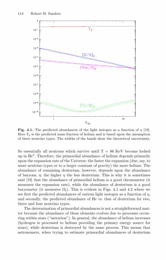
114 Robert H. Sanders
Fig. 4.1. The predicted abundances of the light isotopes as a function of η [19].Here Yp is the predicted mass fraction of helium and is based upon the assumptionof three neutrino types. The widths of the bands show the theoretical uncertainty.
So essentially all neutrons which survive until T = 86 KeV become lockedup in He4. Therefore, the primordial abundance of helium depends primarilyupon the expansion rate of the Universe: the faster the expansion (due, say, tomore neutrino types or to a larger constant of gravity) the more helium. Theabundance of remaining deuterium, however, depends upon the abundanceof baryons, η: the higher η the less deuterium. This is why it is sometimessaid [19] that the abundance of primordial helium is a good chronometer (itmeasures the expansion rate), while the abundance of deuterium is a goodbaryometer (it measures Ωb). This is evident in Figs. 4.1 and 4.2 where wesee first the predicted abundances of various light isotopes as a function of η,and secondly, the predicted abundance of He vs. that of deuterium for two,three and four neutrino types.
The determination of primordial abundances is not a straightforward mat-ter because the abundance of these elements evolves due to processes occur-ring within stars (“astration”). In general, the abundance of helium increases(hydrogen is processed to helium providing the primary energy source forstars), while deuterium is destroyed by the same process. This means thatastronomers, when trying to estimate primordial abundances of deuterium

4 Observational Cosmology 115
Fig. 4.2. The predicted abundance, Yp, of helium (the mass fraction) as a functionof the predicted deuterium abundance for two, three, and four neutrino types [19].The point with error bars is the observed abundances of helium and deuterium.
or helium, must try to find pristine, unprocessed material, in so far as possi-ble. One way to find unprocessed material is to look back at early times, orlarge redshift, before the baryonic material has been recycled through gener-ations of stars. This can be done with quasar absorption line systems, whereseveral groups of observers have been attempting to identify very shallowabsorption lines of deuterium at the same redshift as the much stronger hy-drogen Lyman alpha absorption line systems [20, 21, 22, 23]. It is a difficultobservation requiring the largest telescopes; the lines identified with deu-terium might be mis-identified weak hydrogen or metal lines (incidentally,for an astronomer, any element heavier than helium is a metal). Taking theresults of various groups at face value, the weighted mean value [19] is D/H≈ 2.6±0.3×10⁻⁵. Looking back at Fig. 4.1, we see that this would correspondto η = 6.1 ± 0.6 × 10⁻¹⁰ or Ωbh
2 = 0.022 ± 0.003.A word of caution is necessary here: the values for the deuterium abun-
dance determined by the different groups scatter by more than a factor oftwo, which is considerably larger than the quoted statistical errors (≈ 25%).This indicates that significant systematic effects are present. But it is note-worthy that the angular power spectrum of the CMB anisotropies also yields
116 Robert H. Sanders
an estimate of the baryon abundance; this is encoded in the ratio of theamplitudes of the second to first peak. The value is Ωbh
2 = 0.024 ± 0.001.In other words, the two determinations agree to within their errors. Thisis quite remarkable considering that the first determination involves nuclearprocesses occurring within the first three minutes of the Big Bang, and thesecond involves oscillations of a photon-baryon plasma on an enormous scalewhen the Universe is about 500,000 years old. If this is a coincidence, it istruly an astounding one.
So much for the baryometer, but what about the chronometer helium?Again astronomers are obliged to look for unprocessed material in order toestimate the primordial abundance. The technique of looking at quasar ab-sorption line systems doesn’t work for helium because the absorption linesfrom the ground state are far in the ultraviolet, about 600 A for neutralhelium and, more likely, 300 A from singly ionized helium. This is well be-yond the Lyman limit of hydrogen, where the radiation from the backgroundquasar is effectively absorbed [24]. Here the technique is to look for He emis-sion lines from HII regions (ionized gas around hot stars) in nearby galaxiesand compare to the hydrogen emission lines. But how does one know that thegas is unprocessed? The clue is in the fact that stars not only process hydro-gen into helium, but they also, in the late stages of their evolution, synthesizeheavier elements (metals) in their interiors. Therefore the abundance of heav-ier elements, like silicon, is an indicator of how much nuclear processing theionized gas has undergone. It is observed that the He abundance is correlatedwith the metal abundance; so the goal is to find HII regions with as low ametal abundance as possible, and then extrapolate this empirical correlationto zero metal abundance [25, 26]. The answer turns out to be He/H ≈ 0.24,which is shown by the point with error bars in Fig. 4.2.
This value is embarrassingly low, given the observed deuterium abun-dance. It is obviously more consistent with an expansion rate provided byonly two neutrino types rather than three, but we know that there are cer-tainly three types. Possible reasons for this apparent anomaly are:
1) Bad astronomy: There are unresolved systematic errors in determina-tion of the relative He abundance in HII regions indicated by the fact that theresults of different groups differ by more than the quoted statistical errors [19].The derivation of the helium to hydrogen ratio from the observed He+/H+
ratio requires some understanding of the structure of the HII regions. If thereare relatively cool ionizing stars (T < 35000 K) spatially separated from thehotter stars, there may be relatively less He+ associated with a given abun-dance of H+. Lines of other elements need to be observed to estimate theexcitation temperature; it is a complex problem.
2) New neutrino physics: There may be an asymmetry between neutrinosand anti-neutrinos (something like the baryon- antibaryon asymmetry whichprovides us with the observed Universe). This would manifest itself as achemical potential in the Boltzmann equation giving different equilibriumratios of the various neutrino species [27].

4 Observational Cosmology 117
3) New gravitational physics: any change in the gravitational interactionwhich is effective at early epochs (braneworld effects?) could have a pro-nounced effect on nucleosynthesis. For example, a lower effective constant ofgravity would yield a lower expansion rate and a lower He abundance. Thestandard minimal braneworld correction term, proportional to the square ofthe density [28], goes in the wrong direction.
It is unclear if the low helium abundance is a serious problem for the stan-dard Big Bang. But it is clear that the agreement of the implied baryon abun-dance with the CMB determination is an impressive success, and stronglysupports the assertion that the Hot Big Bang is the correct model for thepre-recombination Universe.
4.5 The Post-recombination Universe:Determination of Ho and to
Certainly the most basic of the cosmological parameters is the present ex-pansion rate, Ho , because this sets the scale of the Universe. Until a fewyears ago, there was a factor of two uncertainty in Ho ; with two separategroups claiming two distinct values, one near 50 km s−1Mpc−1 and the othernearer 100 km s−1Mpc−1, and the errors quoted by both groups were muchsmaller than this factor of two difference. This points out a problem which iscommon in observational cosmology (or indeed, astronomy in general). Oftenthe indicated statistical errors give the impression of great precision, whereasthe true uncertainty is dominated by poorly understood or unknown system-atic effects. That was true in the Hubble constant controversy, and there isno less reason to think that this problem is absent in modern results. I willreturn to this point several times below.
The great leap forward in determination of Ho came with the HubbleSpace Telescope (HST) program on the distance scale. Here a particular kindof variable stars, Cepheid variables, were observed in twenty nearby spiralgalaxies. Cepheids exhibit periodic variations in luminosity by a factor of twoon timescales of 2-40 days. There is a well-determined empirical correlationbetween the period of Cepheids and their mean luminosity– the longer the pe-riod the higher the luminosity. Of course, this period-luminosity relation mustbe calibrated by observing Cepheids in some object with a distance knownby other techniques and this remains a source of systematic uncertainty. Butputting this problem aside, the Hubble Space telescope measured the peri-ods and the apparent magnitudes, without confusion from adjacent brightstars, of a number of Cephieds in each of these relatively nearby galaxies,which yielded a distance determination (4.12). These galaxies are generallytoo close (less than 15 Mpc) to sample the pure Hubble flow, (the Hubbleflow on these scales is contaminated by random motion of the galaxies andsystematic cosmic flows) but these determinations do permit a calibrationof other secondary distance indicators which reach further out, such as su-
118 Robert H. Sanders
pernovae type Ia (SNIa) and the Tully-Fisher relation (the observed tightcorrelation between the rotation velocities of a spiral galaxies and their lumi-nosities). After an enormous amount of work by a number of very competentastronomers [29], the answer turned out to be h = 0.72 ± .10.
As I mentioned there is the known systematic uncertainty of calibrat-ing the period-luminosity relation, but there are other possible systematiceffects that are less well-understood: How can we be certain that the period-luminosity relation for Cepheids is the same in all galaxies? For example, isthis relation affected by the concentration of elements heavier than helium(the metallicity)? In view of such potential problems, other more direct phys-ical methods, which by-pass the traditional “distance ladder” are of interest.Chief among these is the Sunyaev-Zeldovich (S-Z) effect which is relevant toclusters of galaxies [30]. The baryonic mass of clusters of galaxies is primarilyin the form of hot gas, which typically exceeds the mass in the visible galaxiesby more than a factor of two. This gas has a temperature between 107 and108 K (i.e., the sound speed is comparable to the one-dimensional velocitydispersion of the galaxies) and is detected by satellite X-ray telescopes withdetectors in the range of several KeV. The S-Z effect is a small change inthe intensity of the CMB in the direction of such clusters due to Comptonscattering of CMB photons by thermal electrons (classical electron scatteringwould, of course, produce no intensity change). Basically, CMB photons aremoved from the Rayleigh-Jeans part of the black body spectrum to the Wienpart, so the effect is observable as a spectral distortion of the black bodyspectrum in the range of 100 to 300 GHz. It is a small effect (on the order of0.4 milli Kelvin) but still 5 to 10 times larger than the intrinsic anisotropiesin the CMB.
By measuring the amplitude of the S-Z effect one determines an opticaldepth
τ = σnel , (4.22)
where σ is the frequency dependent cross section, l is the path length, and ne
is the electron density. Because these same clusters emit X-rays via thermalbremsstrahlung, we may also determine, from the observed X-ray intensity,an emission measure:
E = ne2l , (4.23)
Here we have two equations for two unknowns, ne and l. This is simplifyingthe actual calculation because ne is a function of radius in the cluster. Know-ing l and the angular diameter of the cluster θ we can then calculate theangular size distance to the cluster via (4.11). Hence, the Hubble parameteris given by Ho = v/DA where v is the observed recession velocity of the clus-ter. All of this assumes that the clusters have a spherical shape on average,so the method needs to be applied to a number of clusters. Even so biases arepossible if clusters have more typically a prolate shape or an oblate shape,or if the X-ray emitting gas is clumpy. Overall, for a number of clusters [31]
4 Observational Cosmology 119
the answer turns out to be h = 0.6, somewhat smaller than the HST distanceladder method, but the systematic uncertainties remain large.
A second direct method relies on time delays in gravitational lenses [32].Occasionally, a distant quasar (the source) is lensed by an intervening galaxy(the lens) into multiple images; that is to say, we observe two or more imagesof the same background object separated typically by one or two seconds ofarc. This means that there are two or more distinct null geodesics connectingus to the quasar with two or more different light travel times. Now a number ofthese quasars are intrinsically variable over time scales of days or months (notperiodic but irregular variables). Therefore, in two distinct images we shouldobserve the flux variations track each other with a time delay. This measureddelay is proportional to the ratio DlDs/Dls where these are the angular sizedistances to the lens, the source, and the lens to the source. Since this ratio isproportional to Ho
−1, the measured time delay, when combined with a massmodel for the lens (the main source of uncertainty in the method), providesa determination of the Hubble parameter. This method, applied to severallenses [33, 34], again tends to yield a value of h that is somewhat smaller thanthe HST value, i.e., ≈ 0.6. In a recent summary [35] it is claimed that, forfour cases where the lens is an isolated galaxy, the result is h = 0.48 ± .03,if the overall mass distribution in each case can be represented by a singularisothermal sphere. On the other hand, in a well-observed lens where themass distribution is constrained by observations of stellar velocity dispersion[36], the implied value of h is 0.75+.07
−.06. Such supplementary observations areimportant because the essential uncertainty with this technique is in theadopted mass model of the lens.
It is probably safe to say that h ≈ 0.7, with an uncertainty of 0.10 andperhaps a slight bias toward lower values, but the story is not over as S-Z andgravitational lens determinations continue to improve. This is of considerableinterest because the best fit to the CMB anisotropies observed by WMAPimplies that h = 0.72 ± .05 in perfect agreement with the HST result. Withthe S-Z effect and lenses, there remains the possibility of a contradiction.
With h = .70, we find a Hubble time of tH = 14 Gyr. Now in FRWcosmology, the age of the Universe is to = ftH where f is a number depend-ing upon the cosmological model. For an Einstein-de Sitter Universe (i.e.,Ωk = 0, ΩQ = 0, Ωm = 1) f = 2/3 which means that to = 9.1 Gyr. Foran empty negatively curved Universe, f = 1 which means that the age isthe Hubble time. Generally, models with a dominant vacuum energy den-sity (ΩQ ≈ 1, w ≈ −1) are older (f ≥ 1) and for the concordance model,f = 0.94. Therefore, independent determinations of the age of the Universeare an important consistency test of the cosmology.
It is reasonable to expect that the Universe should be older than the oldeststars it contains, so if we can measure the ages of the oldest stars, we have, atleast, a lower limit on the age of the Universe. Globular star clusters are oldstellar systems in the halo of our own galaxy; these systems are distributed ina roughly spherical region around the galactic disk and have low abundances

120 Robert H. Sanders
of heavy elements suggesting they were formed before most of the stars inthe disk. If one can measure the luminosity of the most luminous, Lu, un-evolved stars in a globular cluster (that is, stars still burning hydrogen intheir cores), then one may estimate the age. That is because this luminosityis correlated with age: a higher Lu means a lower age. Up to about five yearsago, this method yielded globular cluster ages of tgc ≈ 14 ± 2 Gyr, which,combined with the Hubble parameter discussed above, would be in directcontradiction with the Einstein-de Sitter Ωm = 1 Universe. But about fiveyears ago the Hipparchus satellite began to return accurate parallaxes forhundreds of nearby stars which led to a recalibration of the entire distancescale. All distances outside the solar system increased by about 10% (in fact,the entire Universe suddenly grew by this same factor leading to a decreasein the HST value for the Hubble parameter from about 80 to 72). This meantthat the globular clusters were further away, that Lu was 20% larger larger,and the globular clusters were correspondingly younger: tgc ≈ 11.5 ± 1.3Gyr. If we assume that the Universe is about 1 Gyr older than the globularclusters, then the age of the Universe becomes 12.5 ± 2 Gyr [37] which isalmost consistent with the Einstein-de Sitter Universe. At least there is nolonger any compelling time scale argument for a non zero vacuum energydensity, ΩQ > 0.
A second method for determining the ages of stars is familiar to all physi-cists, and that is radioactive dating. This has been done recently by observa-tions of a U238 line in a metal-poor galactic star (an old star). Although theiron abundance in this star is only 1/800 that of the sun, the abundances ofa group of rare earth metals known as r-process elements are enhanced. Ther-process is rapid neutron absorption onto iron nuclei (rapid compared to thetimescale for subsequent β decay) which contributes to certain abundancepeaks in the periodic table and which occurs in explosive events like super-novae. This means that this old star was formed from gas contaminated byan even older supernova event; i.e., the uranium was deposited at a definitetime in the past. Now U238 is unstable with a half life of 4.5 Gyr which makesit an ideal probe on cosmological times scales. All we have to do is comparethe observed abundance of U238 to that of a stable r-process element (in thiscase osmium), with what is expected from the r-process. The answer for theage of this star (or more accurately, the SN which contaminated the gas outof which the star formed) is 12.5 ±3 Gyr, which is completely consistent withthe globular cluster ages [38].
If we take 0.6 < h < 0.7, and 9.5 Gyr < to < 15.5 Gyr this implies that0.59 < Hoto < 1.1. This is consistent with a wide range of FRW cosmologiesfrom Einstein-de Sitter to the concordance model. That is to say, indepen-dent measurements of Ho and to are not yet precise enough to stand as aconfirmation or contradiction to the WMAP result.

4 Observational Cosmology 121
4.6 Looking for Discordance: The Classical Tests
4.6.1 The Angular Size Test
The first of the classical cosmological tests we will consider is the angular sizetest. Here one measures the angular size of a standard meter stick (hopefully)as a function of redshift; different FRW cosmologies make different predic-tions, but basically, for all FRW models θ(z) first decreases as 1/z (as wouldbe expected in a Euclidean universe) and then increases with z. This is be-cause the angular size distance is given by DA = r/(1 + z) but the radialcomoving coordinate approaches a finite value as z → ∞. The angular sizedistance reaches a maximum at a redshift between 1 and 2 and then decreasesagain.
When giant radio galaxies at large redshift were discovered in the 1960’sthere was considerable optimism that these could be used as an angular sizecosmological probe. Radio galaxies typically have a double-lobe structurewith the radio emitting lobes straddling the visible galaxy; these lobes canextend hundreds of kpc beyond the visible object. Such a linear structuremay be oriented at any angle to the observer’s line-of-sight, so one needs tomeasure the angular sizes of a number of radio galaxies in a given redshift binand only consider the largest ones, i.e., those likely to be nearly perpendicularto the line-of-sight.
The result of all this work was disappointing. It appeared that the angularsize of radio sources kept decreasing with redshift just as one would expect fora pure Euclidean universe [39]. The obvious problem, that plagues all classicaltests, is that of evolution. Very likely, these radio galaxies are not standardmeter sticks at all, but that they were actually smaller at earlier epochs thannow. This would be expected, because such objects are thought to result fromjets of relativistic particles ejected from the nucleus of the parent galaxy inopposite directions. The jets progress through the surrounding intergalacticmedium at a rate determined by the density of that medium, which, of course,was higher at larger redshift.
But there is another class of radio sources that would be less susceptible tosuch environmental effects: the compact radio sources. These are objects, ona scale of milli-arc-seconds, typically associated with distant quasars, that areobserved with radio interferometers having global baselines. The morphologyis that of a linear jet with lengths typically less than 30 or 40 pc, so thesewould presumably be emission from the jets of relativistic particles deep inthe galactic nucleus near the central engine producing them. The intergalacticmedium, and its cosmological evolution, would be expected to have no effecthere [40].
The result of plotting the median angular size of about 150 of these sourcesas a function of redshift is shown on a log-log plot in Fig. 4.3 [41]. Also shownare the predicted relations for three flat cosmologies (Ωk = 0) with Ωm = 0.9,0.3, 0.1, the remainder being in a cosmological constant (the middle curve

122 Robert H. Sanders
Fig. 4.3. The median angular size vs. redshift (log-log plots) for 145 compactradio sources in 12 redshift bins. The curves are the three flat cosmological models:dashed, ΩΛ = 0.9; solid, ΩΛ = 0.7 (concordance), dotted, ΩΛ = 0.1. The physicalsize of the sources (20-40 pc) has been chosen for the best fit.
is the concordance model). In each case the linear size of the compact radiosources was chosen to achieve the best fit to the data.
It is evident that the general property of FRW models (that the angu-lar size of a standard meter stick should begin to increase again beyond aredshift of about 1.5) is present in this data. However, no statistical test ormaximum likelihood analysis is necessary to see that all three models fit thedata equally well. This is basically an imprecise cosmological test and cannotbe improved, particularly considering that these objects may also evolve insome unknown way with cosmic time. Looking at the figure, one may noticethat measurement of angular sizes for just a few objects at lower redshiftmight help distinguish between models. However, there are very few suchobjects at lower redshift, and these have a much lower intrinsic radio powerthan those near redshift one. It is dangerous to include these objects on sucha plot because they are probably of a very different class.
4.6.2 The Modern Angular Size Test: CMB-ology
Although it is not my purpose here to discuss the CMB anisotropies (see A.Challinor’s contribution), it is necessary to say a few words on the preferredangular scale of the longest wavelength acoustic oscillations, the “first peak”,because this is now the primary evidence for a flat Universe (Ωk = 0). InFig. 4.4 we see again the now very familiar plot of the angular power spectrumof anisotropies as observed by WMAP [43] (in my opinion, of all the WMAPpapers, this reference provides the clearest discussion of the physics behindthe peak amplitudes and positions). The solid line is the concordance model,
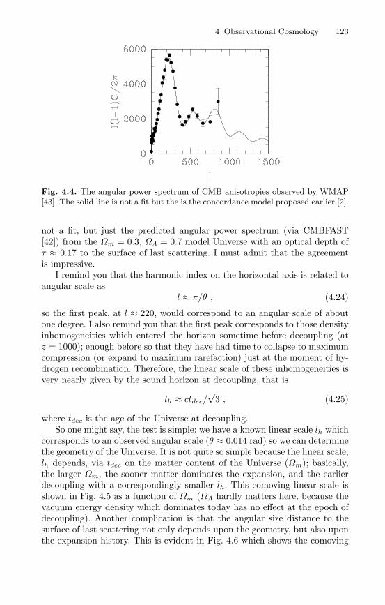
4 Observational Cosmology 123
Fig. 4.4. The angular power spectrum of CMB anisotropies observed by WMAP[43]. The solid line is not a fit but the is the concordance model proposed earlier [2].
not a fit, but just the predicted angular power spectrum (via CMBFAST[42]) from the Ωm = 0.3, ΩΛ = 0.7 model Universe with an optical depth ofτ ≈ 0.17 to the surface of last scattering. I must admit that the agreementis impressive.
I remind you that the harmonic index on the horizontal axis is related toangular scale as
l ≈ π/θ , (4.24)
so the first peak, at l ≈ 220, would correspond to an angular scale of aboutone degree. I also remind you that the first peak corresponds to those densityinhomogeneities which entered the horizon sometime before decoupling (atz = 1000); enough before so that they have had time to collapse to maximumcompression (or expand to maximum rarefaction) just at the moment of hy-drogen recombination. Therefore, the linear scale of these inhomogeneities isvery nearly given by the sound horizon at decoupling, that is
lh ≈ ctdec/√
3 , (4.25)
where tdec is the age of the Universe at decoupling.So one might say, the test is simple: we have a known linear scale lh which
corresponds to an observed angular scale (θ ≈ 0.014 rad) so we can determinethe geometry of the Universe. It is not quite so simple because the linear scale,lh depends, via tdec on the matter content of the Universe (Ωm); basically,the larger Ωm, the sooner matter dominates the expansion, and the earlierdecoupling with a correspondingly smaller lh. This comoving linear scale isshown in Fig. 4.5 as a function of Ωm (ΩΛ hardly matters here, because thevacuum energy density which dominates today has no effect at the epoch ofdecoupling). Another complication is that the angular size distance to thesurface of last scattering not only depends upon the geometry, but also uponthe expansion history. This is evident in Fig. 4.6 which shows the comoving

124 Robert H. Sanders
Fig. 4.5. The comoving linear scale of the perturbation corresponding to the firstpeak as a function of Ωm
Fig. 4.6. The angular size distance (Gpc) to the last scattering surface (z = 1000)as a function of Ωm for various values of Ωtot.
angular size distance (in Gpc) to the surface of last scattering as a functionof Ωm for three values of Ωtot = Ωm +ΩΛ (i.e., Ωk = 1−Ωtot). Note that thecomoving angular size distance, DA(1+z), is the same as the radial comovingcoordinate r.
We can combine Figs. 4.5 and 4.6 to plot the expected angular size (orharmonic index) of the first peak as a function of Ωm and Ωtot, and thisis shown in Fig. 4.7 with the dashed line giving the observed l of the firstpeak. We see that a model with Ωtot ≥ 1.1 (a closed universe) is clearlyruled out, but it would be possible to have an open model with Ωtot = 0.9and Ωm = 0.8 from the position of the first peak alone; the predicted peakamplitude, however, would be about 40% too low. The bottom line of all ofthis is that the position of the first peak does not uniquely define the geometryof the Universe because of a degeneracy with Ωm (I haven’t mentioned thedegeneracy with h taken here to be 0.72). To determine whether or not welive in a flat Universe we need an independent handle on Ωm and that is

4 Observational Cosmology 125
Fig. 4.7. The harmonic index expected for the first peak as a function of Ωm forvarious values of Ωtot.
provided, in WMAP data, by the amplitudes of the first two peaks (the morenon-baryonic matter, the deeper the forming potential wells, and the lowerthe amplitudes). From this it is found that Ωm ≈ 0.3, and from Fig. 4.7 wesee that the model Universe should be near flat (Ωtot ≈ 1.0). Of course if theUniverse is near flat with Ωm = 0.3 then the rest must be in dark energy;this is the indirect evidence from the CMB anisotropies for dark energy.
I just add here that the observed peak amplitudes (given the optical depthto z = 1000 determined from WMAP polarization results [44]), is taken nowas definitive evidence for CDM. However, alternative physics which affectsthe amplitude and positions of peaks (e.g. [3]) could weaken this conclusion,as well as affect the derived cosmological parameters. Even taking the peakamplitudes as prima facie evidence for the existence of cold dark matter, it isonly evidence for CDM at the epoch of recombination (z = 1000) and not inthe present Universe. To address the cosmic coincidence problem, models havebeen suggested in which dark matter transmutes into dark energy (e.g. [45]).
Now I turn to the direct evidence for dark energy.
4.6.3 The Flux-Redshift Test: Supernovae Ia
Type I supernovae are thought to be nuclear explosions of carbon/oxygenwhite dwarfs in binary systems. The white dwarf (a stellar remnant supportedby the degenerate pressure of electrons) accretes matter from an evolvingcompanion and its mass increases toward the Chandrasekhar limit of about1.4 M (this is the mass above which the degenerate electrons become rel-ativistic and the white dwarf unstable). Near this limit there is a nucleardetonation in the core in which carbon (or oxygen) is converted to iron. Anuclear flame propagates to the exterior and blows the white dwarf apart(there are alternative models but this is the favored scenario [46]).
These events are seen in both young and old stellar populations; for ex-ample, they are observed in the spiral arms of spiral galaxies where there is

126 Robert H. Sanders
active star formation at present, as well as in elliptical galaxies where vigor-ous star formation apparently ceased many Gyr ago. Locally, there appearsto be no difference in the properties of SNIa arising in these two different pop-ulations, which is important because at large redshift the stellar populationis certainly younger.
The peak luminosity of SNIa is about 1010 L which is comparable to thatof a galaxy. The characteristic decay time is about one month which, in themore distant objects, is seen to be stretched by 1+z as expected. The lightcurve has a characteristic form and the spectra contain no hydrogen lines, sogiven reasonable photometric and spectroscopic observations, they are easyto identify as SNIa as opposed to type II supernovae; these are thought to beexplosions of young massive stars and have a much larger dispersion in peakluminosity [47].
The value of SNIa as cosmological probes arises from the high peak lumi-nosity as well as the observational evidence (locally) that this peak luminosityis the sought-after standard candle. In fact, the absolute magnitude, at peak,varies by about 0.5 magnitudes which corresponds to a 50%-60% variation inluminosity; this, on the face of it, would make them fairly useless as standardcandles. However, the peak luminosity appears to be well-correlated with de-cay time: the larger Lpeak, the slower the decay. There are various ways ofquantifying this effect [47], such as
MB ≈ 0.8(∆m15 − 1.1) − 19.5 , (4.26)
where MB is the peak absolute magnitude and ∆ m15 is the observed changein apparent magnitude 15 days after the peak [48]. This is an empirical re-lationship, and there is no consensus about the theoretical explanation, but,when this correction is applied it appears that ∆Lpeak < 20%. If true, thismeans that SNIa are candles that are standard enough to distinguish betweencosmological models at z ≈ 0.5.
In a given galaxy, supernovae are rare events (on a human time scale,that is), with one or two such explosions per century. But if thousands ofgalaxies can be surveyed on a regular and frequent basis, then it is possibleto observe several events per year over a range of redshift. About 10 yearsago two groups began such ambitious programs [49, 50]; the results have beenfantastically fruitful and have led to a major paradigm shift.
The most recent results are summarized in [51]: at present, about 230SNIa have been observed out to z = 1.2. The bottom line is that SNIa are10% to 20% fainter at z ≈ 0.5 than would be expected in an empty (Ωtot = 0)non-accelerating Universe. But, significantly, at z ≥ 1 the supernovae appearto become brighter again relative to the non-accelerating case; this shouldhappen in the concordance model at about this redshift because it is herethat the cosmological constant term in the Friedmann equation (4.10) firstbegins to dominate over the matter term. This result is shown in Fig. 4.8which is a plot of the median ∆m, the observed deviation from the non-accelerating case, in various redshift bins as a function of redshift (i.e., the
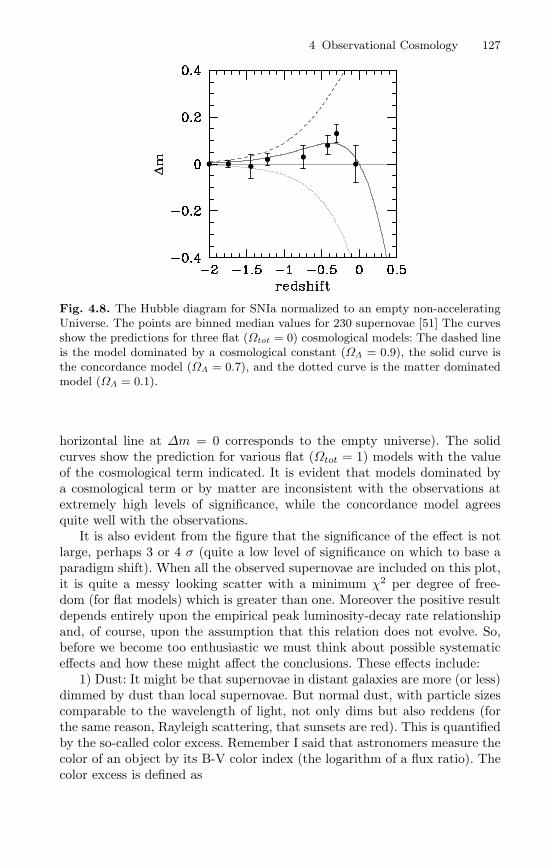
4 Observational Cosmology 127
Fig. 4.8. The Hubble diagram for SNIa normalized to an empty non-acceleratingUniverse. The points are binned median values for 230 supernovae [51] The curvesshow the predictions for three flat (Ωtot = 0) cosmological models: The dashed lineis the model dominated by a cosmological constant (ΩΛ = 0.9), the solid curve isthe concordance model (ΩΛ = 0.7), and the dotted curve is the matter dominatedmodel (ΩΛ = 0.1).
horizontal line at ∆m = 0 corresponds to the empty universe). The solidcurves show the prediction for various flat (Ωtot = 1) models with the valueof the cosmological term indicated. It is evident that models dominated bya cosmological term or by matter are inconsistent with the observations atextremely high levels of significance, while the concordance model agreesquite well with the observations.
It is also evident from the figure that the significance of the effect is notlarge, perhaps 3 or 4 σ (quite a low level of significance on which to base aparadigm shift). When all the observed supernovae are included on this plot,it is quite a messy looking scatter with a minimum χ2 per degree of free-dom (for flat models) which is greater than one. Moreover the positive resultdepends entirely upon the empirical peak luminosity-decay rate relationshipand, of course, upon the assumption that this relation does not evolve. So,before we become too enthusiastic we must think about possible systematiceffects and how these might affect the conclusions. These effects include:
1) Dust: It might be that supernovae in distant galaxies are more (or less)dimmed by dust than local supernovae. But normal dust, with particle sizescomparable to the wavelength of light, not only dims but also reddens (forthe same reason, Rayleigh scattering, that sunsets are red). This is quantifiedby the so-called color excess. Remember I said that astronomers measure thecolor of an object by its B-V color index (the logarithm of a flux ratio). Thecolor excess is defined as

128 Robert H. Sanders
E(B − V ) = (B − V )obs − (B − V )int , (4.27)
where obs means the observed color index and int means the intrinsic colorindex (the color the object would have with no reddening). In our own galaxyit is empirically the case that the magnitudes of absorption is proportionalto this color excess, i.e.,
AV = RV E(B − V ) , (4.28)
where RV is roughly constant and depends upon average grain properties.So assuming that the dust in distant galaxies is similar to the dust in ourown, it should be possible to estimate and correct for the dust obscuration.Significantly [49], it appears that there is no difference between E(B-V) forlocal and distant supernovae. This implies that the distant events are notmore or less obscured than the local ones.
2) Grey dust: It is conceivable (but unlikely) that intergalactic space con-tains dust particles which are significantly larger than the wavelength of light.Such particles would dim but not redden the distant supernovae and so wouldbe undetectable by the method described above [52]. It is here that the veryhigh redshift supernovae (z > 1) play an important role. If this is the causeof the apparent dimming we might expect that the supernovae would notbecome brighter again at higher redshift.
3) Evolution: It is possible that the properties of these events may haveevolved with cosmic time. As I mentioned above, the SN exploding at highredshift come from a systematically younger stellar population than the ob-jects observed locally. Moreover, the abundance of metals was smaller in theearlier Universe than now; this evolving composition, by changing the opac-ity in the outer layers or the composition of the fuel itself could lead to asystematic evolution in peak luminosity. Here it is important to look for ob-servational differences between local and distant supernovae, and there seemto be no significant differences in most respects, the spectrum or the lightcurve. There is, however, a suggestion that distant supernovae are intrinsi-cally bluer than nearby objects [47]. If this effect is verified, then it could notonly point to a systematic difference in the objects themselves, but could alsohave lead to an underestimate of the degree of reddening in the distant SN. Itis difficult, in general, to eliminate the possibility that the events themselveswere different in the past and that this could mimic the effect of a cosmolog-ical constant [53]; a deeper theoretical understanding of the SNIa process isrequired in order to realistically access this possibility.
4) Sample evolution: The sample of SN selected at large redshift may dif-fer from the nearby sample that is used, for example, to calibrate the peakluminosity-decline rate correlation. There does appear to be an absence, atlarge redshift, of SN with very slowly declining light curves– which is to say,very luminous SN that are seen locally. Perhaps a class of more luminousobjects is missing in the more distant Universe due to the fact that these SNemerge from a systematically younger stellar population. One would hope

4 Observational Cosmology 129
that the luminosity-decline rate correlation would correct for this effect, as-suming, of course, that this relation itself does not evolve.
5) Selection biases: There is a dispersion in the luminosity-decline raterelationship, and in a flux-limited sample, one tends to select the higher lu-minosity objects. Astronomers call this sort of bias the “Malmquist effect”and it is always present in such observational data. Naively, one would expectsuch a bias to lead to an underestimate of the true luminosity, and, there-fore an underestimate luminosity distance; the bias actually diminishes theapparent acceleration. But there is another effect which is more difficult toaccess: The most distant supernovae are being observed in the UV of theirown rest frame. SNIa are highly non-uniform in the UV, and K-correctionsare uncertain. This could introduce systematic errors at the level of a fewhundredths of a magnitudes [51].
We see that there are a number of systematic effects that could bias theseresults. A maximum likelihood analysis over the entire sample [51], confirmsearlier results that the confidence contours in Ωm-ΩΛ space are stretchedalong a line ΩΛ = 1.4Ωm + 0.35 and that the actual best fit is provided by amodel with Ωm ≈ 0.7 and ΩΛ ≈ 1.3, not the concordance model. Of course, ifwe add the condition that Ωtot = 1 (a flat Universe) then the preferred modelbecomes the concordance model. In [51] it is suggested that this apparentdeviation is due to the appearance of one or more of the systematic effectsdiscussed above near z = 1 at the level of 0.04 magnitudes.
The result that SNIa are systematically dimmer near z = 0.5 than ex-pected in a non-accelerating Universe is robust. At the very least it can beclaimed with reasonable certainty that the Universe is not decelerating atpresent. However, given the probable presence of systematic uncertainties atthe level of a few hundredths of a magnitude, it is difficult to constrain theequation of state (w) of the dark energy or its evolution (dw/dt) until theseeffects are better understood. I will just mention that lines of constant age,toHo, are almost parallel to the best fit line in the Ωm-ΩΛ plane mentionedabove. This then gives a fairly tight constraint on the age in Hubble times[51]; i.e. toHo = 0.96 ± 0.4, which is consistent with the WMAP result. In anear flat Universe this rules out the dominance of matter and requires a darkenergy term.
4.6.4 Number Counts of Faint Galaxies
The final classical test I will discuss is that of number counts of distantobjects, what radio astronomers call the log(N)-log(S) test. Basically onecounts the number of galaxies N brighter than a certain flux limit S. If we livedin a static Euclidean universe, then the number of galaxies out to distance Rwould be N ∝ R3 but the flux is related to R as S ∝ R−2. This implies thatN ∝ S−3/2 or log(N) = −3/2 log(S) + const = 0.6m+ const. where m is themagnitude corresponding to the flux S.

130 Robert H. Sanders
Fig. 4.9. The log of the incremental volume per incremental redshift (in units ofthe Hubble volume) as a function of redshift for the three flat cosmological models.
But we do not live in a static Euclidean universe; we live in an evolvinguniverse with a non-Euclidean geometry where the differential number countsprobe dV(z), the comoving volume as a function of redshift. In Fig. 4.9 we seelog(dV/dz) as a function of redshift for three different(Ωtot = 1) cosmologicalmodels: the matter dominated Universe, the cosmological constant dominatedUniverse, and the concordance model. For small z, dV/dz increases as z2 forall models as would be expected in a Euclidean Universe, but by redshift one,the models are obviously diverging, with the models dominated by a cosmo-logical constant having a larger comoving incremental volume. Therefore ifwe can observe faint galaxies extending out to a redshift of one or two, wemight expect number counts to provide a cosmological probe.
There is a long history of counting objects as a function of flux or red-shift. Although cosmological conclusions have been drawn (see, e.g. [54]), theoverall consensus is that this is not a very good test because the galaxy popu-lation evolves strongly with redshift. Galaxies evolve because stars evolve. Inthe past, the stellar populations were younger and contained relatively moremassive, luminous stars. Therefore we expect galaxies to be more luminous athigher redshift. It is also possible that the density of galaxies evolves becauseof merging, as would be consistent with the preferred model of hierarchicalstructure formation in the Universe.
The distribution of galaxies by redshift can be used, to some extent, tobreak this degeneracy between evolution and cosmology. If we can measurethe redshifts of galaxies with infrared magnitudes between 23 and 26, forexample, that distribution will be skewed toward higher redshift if there ismore luminosity evolution.

4 Observational Cosmology 131
Fig. 4.10. The solid points are the faint galaxy number counts from the HubbleDeep Fields (north and south [56, 57]) and the star shaped points are the numbercounts from ground based data. The curves are the no-evolution predictions fromthree flat cosmological models.
I have recently reconsidered the number counts of the faint galaxies in theHubble Deep Fields, north and south [56, 57]. These are two separate smallpatches of empty sky observed with the Hubble Space Telescope down to avery low flux limit– about mI = 30 (the I band is a far red filter centeredaround 8000 angstroms). The differential number counts are shown by thesolid round points in Fig. 4.10 where ground based number counts at faintermagnitudes are also shown by the starred points.
For this same sample of galaxies, there are also estimates of the redshiftsbased upon the galaxy colors, the so called photometric redshifts [58]. Inorder to calculate the expected number counts and redshift distribution onemust have some idea of the form of the luminosity function, the distributionof galaxies by redshift. Here, like everyone else, I have have assumed that thisform is given by the Schechter function [59]:
N(L)dL = No(L/L∗)−αexp(−L/L∗)dL , (4.29)
which is characterized by three parameters: α, a power law at low luminosi-ties, L∗ a break-point above which the number of galaxies rapidly decreases,and No a normalization. I take this form because the overall galaxy distri-bution by luminosity at low redshifts is well fit by such a law [60], so I amassuming that at least the form of the luminosity function does not evolvewith redshift.
But when I consider faint galaxies at high redshift in a particular bandI have to be careful to apply the K-correction mentioned above; that is, Imust correct the observed flux in that band to the rest frame. Making this
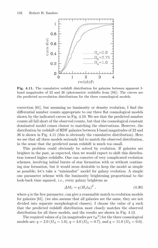
132 Robert H. Sanders
Fig. 4.11. The cumulative redshift distribution for galaxies between apparent I-band magnitudes of 23 and 26 (photometric redshifts from [58]). The curves arethe predicted no-evolution distributions for the three cosmological models.
correction [61], but assuming no luminosity or density evolution, I find thedifferential number counts appropriate to our three flat cosmological modelsshown by the indicated curves in Fig. 4.10. We see that the predicted numbercounts all fall short of the observed counts, but that the cosmological constantdominated model comes closest to matching the observations. However, thedistribution by redshift of HDF galaxies between I-band magnitudes of 22 and26 is shown in Fig. 4.11 (this is obviously the cumulative distribution). Herewe see that all three models seriously fail to match the observed distribution,in the sense that the predicted mean redshift is much too small.
This problem could obviously be solved by evolution. If galaxies arebrighter in the past, as expected, then we would expect to shift this distribu-tion toward higher redshifts. One can conceive of very complicated evolutionschemes, involving initial bursts of star formation with or without continu-ing star formation, but it would seem desirable to keep the model as simpleas possible; let’s take a “minimalist” model for galaxy evolution. A simpleone parameter scheme with the luminosity brightening proportional to thelook-back time squared, i.e., every galaxy brightens as
∆MI = q (Hotlb)2, (4.30)
where q is the free parameter, can give a reasonable match to evolution modelsfor galaxies [61]. (we also assume that all galaxies are the same, they are notdivided into separate morphological classes). I choose the value of q suchthat the predicted redshift distribution most closely matches the observeddistribution for all three models, and the results are shown in Fig. 4.12.
The required values of q (in magnitudes per tH2) for the three cosmologicalmodels are: q = 2.0 (ΩΛ = 1.0), q = 3.0 (ΩΛ = 0.7), and q = 11.0 (ΩΛ = 0.0).
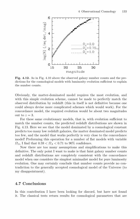
4 Observational Cosmology 133
Fig. 4.12. As in Fig. 4.10 above the observed galaxy number counts and the pre-dictions for the cosmological models with luminosity evolution sufficient to explainthe number counts.
Obviously, the matter-dominated model requires the most evolution, andwith this simple evolution scheme, cannot be made to perfectly match theobserved distribution by redshift (this in itself is not definitive because onecould always devise more complicated schemes which would work). For theconcordance model, the required evolution would be about two magnitudesout to z = 3.
For these same evolutionary models, that is, with evolution sufficient tomatch the number counts, the predicted redshift distributions are shown inFig. 4.13. Here we see that the model dominated by a cosmological constantpredicts too many low redshift galaxies, the matter dominated model predictstoo few, and the model that works perfectly is very close to the concordancemodel! Preforming this operation for a number of flat models with variableΩΛ, I find that 0.59 < ΩΛ < 0.71 to 90% confidence.
Now there are too many assumptions and simplifications to make thisdefinitive. The only point I want to make is that faint galaxy number countsand redshift distributions are completely consistent with the concordancemodel when one considers the simplest minimalist model for pure luminosityevolution. One may certainly conclude that number counts provide no con-tradiction to the generally accepted cosmological model of the Universe (tomy disappointment).
4.7 Conclusions
In this contribution I have been looking for discord, but have not foundit. The classical tests return results for cosmological parameters that are
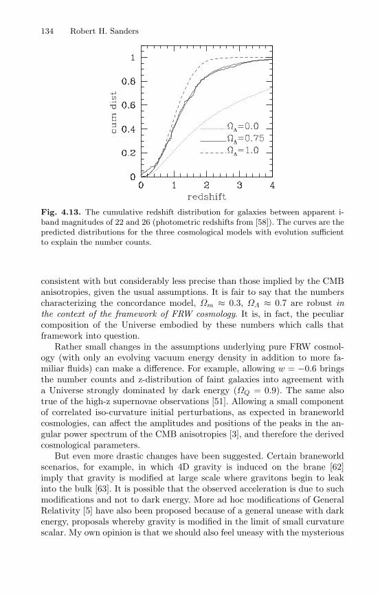
134 Robert H. Sanders
Fig. 4.13. The cumulative redshift distribution for galaxies between apparent i-band magnitudes of 22 and 26 (photometric redshifts from [58]). The curves are thepredicted distributions for the three cosmological models with evolution sufficientto explain the number counts.
consistent with but considerably less precise than those implied by the CMBanisotropies, given the usual assumptions. It is fair to say that the numberscharacterizing the concordance model, Ωm ≈ 0.3, ΩΛ ≈ 0.7 are robust inthe context of the framework of FRW cosmology. It is, in fact, the peculiarcomposition of the Universe embodied by these numbers which calls thatframework into question.
Rather small changes in the assumptions underlying pure FRW cosmol-ogy (with only an evolving vacuum energy density in addition to more fa-miliar fluids) can make a difference. For example, allowing w = −0.6 bringsthe number counts and z-distribution of faint galaxies into agreement witha Universe strongly dominated by dark energy (ΩQ = 0.9). The same alsotrue of the high-z supernovae observations [51]. Allowing a small componentof correlated iso-curvature initial perturbations, as expected in braneworldcosmologies, can affect the amplitudes and positions of the peaks in the an-gular power spectrum of the CMB anisotropies [3], and therefore the derivedcosmological parameters.
But even more drastic changes have been suggested. Certain braneworldscenarios, for example, in which 4D gravity is induced on the brane [62]imply that gravity is modified at large scale where gravitons begin to leakinto the bulk [63]. It is possible that the observed acceleration is due to suchmodifications and not to dark energy. More ad hoc modifications of GeneralRelativity [5] have also been proposed because of a general unease with darkenergy, proposals whereby gravity is modified in the limit of small curvaturescalar. My own opinion is that we should also feel uneasy with the mysterious
4 Observational Cosmology 135
non-baryonic cold dark matter, because the only evidence for its existence, atpresent, is its gravitational influence; when the theory of gravity is modifiedto eliminate dark energy, it might also be found that the need for dark mattervanishes.
In general, more attention is being given to so-called infrared modifica-tions of gravity (e.g. [64]), and this is a positive development. High energymodifications, that affect the evolution of the early Universe, are, as we haveseen, strongly constrained by considerations of primordial nucleosynthesis(now, in combination with the CMB results). It is more likely that mod-ifications play a role in the late, post-recombination evolution of the Uni-verse, where the peculiarities of the concordance model suggest that they areneeded. The fact that the same rather un-natural values for the comparabledensities of dark energy and matter keep emerging in different observationalcontexts may be calling attention to erroneous underlying assumptions ratherthan to the actual existence of these “ethers”.
Convergence toward a parameterized cosmology is not, without deeperunderstanding, sufficient reason for triumphalism. Rather, it should be amotivation to look more carefully at the possible systematic effects in theobservations and to question more critically the underlying assumptions ofthe models.
Acknowledgements
I thank Rien van de Weygaert, Ole Moller, Moti Milgrom, Art Wolfe, Ja-cob Bekenstein, and Scott Trager for useful comments on the manuscript.I also thank Gary Steigman, Wendy Freedman, and Luis Ho for permissionto use Figs. 4.1 and 4.2. I am very grateful to the organizers of the SecondAegean Summer School on the Early Universe, and especially, Lefteris Pa-pantonopoulos, for all their work and for inviting me to the very pleasantisland of Syros.
References
1. D.N. Spergel, et al., Astrophys. J. Suppl., 148, 175 (2003), astro-ph/0302209.2. J.P. Ostriker, P.J. Steinhardt, Nature 377, 600 (1995).3. R. Maartens, gr-qc/0312059.4. Deffayet C, Phys. Lett. B 502, 199 (2001).5. S.M. Carroll, V. Duvvuri, M. Trodden, M.S. Turner, astro-ph/0306438 (2003).6. J.F. Navarro, C.S. Frenk, S.D.M. White, Astrophys. J. 462 563 (1996).7. W.J.G. de Blok, S.S. McGaugh, V.C. Rubin, Astron. J., 122, 2396 (2001).8. T. Treu, L.V.E. Koopmans, D.J. Sand, G.P. Smith, R.S. Ellis, To appear in
the proceedings of IAU Symposium 220 “Dark matter in galaxies”, S. Ryder,D.J. Pisano, M. Walker, and K. Freeman eds, astro-ph/0311052.
9. S.M. Carroll, Living Rev.Rel. 4, 1 (2001), astro-ph/0004075.
136 Robert H. Sanders
10. P.J.E. Peebles, B. Ratra’, Rev. Mod. Phys., 75, 559 (2003).11. T. Padmanabhan, hep-th/0212290.12. J.A. Peacock, Phil. Trans. Roy. Soc. Lond., A361 2479 (2003), astro-
ph/0309238.13. H. Hoekstra, H. Yee, M. Gladders, Astrophys. J., 577, 595 (2002).14. M. Milgrom, Astrophys. J., 270, 365 (1983).15. W. Rindler, Essential Relativity, (Heidelberg, Springer-Verlag).16. R.R. Caldwell, Phys. Lett. B545, 23 (2002).17. J.C. Mather et al., Astrophys. J., 512, 511 (1999).18. P. Molaro, S.A. Levshakov, M. Dessauges-Zavadsky, S. D’Odorico, As-
tron.Astrophys., 381, 64 (2002), astro-ph/0111589.19. G. Steigman, Carnegie Observatories Astrophysics Series Vol. 2, ”Measuring
and Modeling the Universe”, W. Freedman ed. (Cambridge, Cambridge Univ.Press) (2003), astro-ph/ 0307244.
20. S. Burles, D. Tytler, Astrophys. J., 499, 699 (1998).21. J.M. O’Meara et al., Astrophys. J., 552, 718 (2001).22. M. Pettini, D.V. Bowen, Astrophys. J., 560, 41 (2001).23. D. Kirkman, et al., Astrophys. J. Suppl, in press (2003), astro-ph/0302006.24. P.Jakobsen et al., Astrophys. J., 417, 528 (1993).25. K. Olive, G. Steigman, Astrophys. J. Supp., 97, 49 (1995).26. Y.I. Izotov, T.X. Thuan, Astrophys. J., 500, 188 (1998).27. V. Barger, J.P. Kneller, P. Langacker, D. Marfatia, G. Steigman, Phys.Lett.
B569 123 (2003), hep-ph/0306061.28. C. Barcelo, M. Visser, Phys.Lett. B482, 183 (2000), hep-th/0004056.29. W.L. Freedman et al., Astrophys. J., 553, 47 (2001).30. R.A. Sunyaev, Ya.B. Zeldovich, Ann. Rev. Astron. Astrophys., 18, 537 (1980).31. J.E. Carlstrom, G.P. Holder, E.D. Reese, Ann.Rev.Astron.Astrophys., 40, 643
(2002).32. S. Refsdal, Mon. Not. RAS, 128, 307 (1964).33. L.L.R. Williams, P. Saha, Astron. J., 119, 439 (2000).34. L.V.E. Koopmans, C.D. Fassnacht, Astrophys. J., 527, 513 (1999).35. C.S. Kochanek, P.L. Schechter, to appear in Measuring and Modeling the Uni-
verse (Carnegie Observatories Astrophysics Series, Vol. 2), ed. W.L. Freedman(2003), astro-ph/0306040.
36. L.V.E. Koopmans et al., Astrophys. J., 599, 70 (2003).37. B. Chaboyer, P. Demarque, P.J. Kernan, L.M. Krauss, Astrophys. J., 494, 96
(1998).38. R. Cayrel et al., Nature, 409, 691 (2001), astro-ph/0104357.39. G.K. Miley, Mon. Not. RAS, 152, 477 (1971).40. K.I. Kellerman, Nature, 361, 134 (1993).41. L.I. Gurvits, K.I. Kellerman, S. Frey, Astron. Astrophys, 342, 378 (1999).42. U. Seljak, M. Zeldarriaga, Astrophys. J., 469, 437 (1996).43. L. Page et al., Astrophys. J. Suppl., 148, 233 (2003).44. A. Kogut et al., Astrophys. J. Suppl., 148, 161 (2003).45. B.A. Bassett, M. Kunz, D. Parkinson, C. Ungarelli, Phys. Rev., D68, 043504
(2003).46. D. Branch, Ann. Rev. Astron. Astrophys., 36, 17 (1998).47. B. Leibundgut, Ann. Rev. Astron. Astrophys, 39, 67 (2001).48. M. Hamuy, M.M. Phillips, R.A. Schommer, N.B. Suntzeff, Astron. J., 112, 2391
(1996).
4 Observational Cosmology 137
49. Perlmutter S, et al., Astrophys. J., 517, 565 (1999).50. P.M. Garnevitch et al. , Astrophys. J., 493, 53 (1998).51. J.L. Tonry et al., Astrophys. J., 594, 1 (2003), astro-ph/0305008.52. A. Aguirre, Z. Haiman, Astrophys. J., 532, 28 (2000).53. P.S. Drell, T.J. Loredo, I. Wasserman, Astrophys. J., 530, 593 (2000).54. M. Fukugita, F. Takahara, K. Yamashita, Y. Yoshi, Astrophys. J., 361, L1
(1990).55. Y. Yoshii, F. Takahara, Astrophys. J., 346, 28 (1989).56. R.E. Williams et al., Astron. J., 112, 1335 (1996).57. S. Casertano et al., Astron. J., 120, 247 (2000).58. A. Fernandez-Soto, K.M. Lanzetta, A. Yahil, Astrophys. J., 513, 34 (1999).59. P.L. Schechter, Astrophys. J., 203, 297 (1976).60. M.R. Blanton et al., Astron. J., 121, 2358 (2001).61. B.M. Poggianti, Astron. Astrophys. Suppl, 122, 399 (1997).62. G. Dvali, G. Gabadadaze, M. Porrati, Phys. Lett., B485, 208 (2000), hep-
th/0005016.63. C. Deffayet, G. Dvali, G. Gabadadze, Phys. Rev. D65 044023 (2002), astro-
ph/0105068.64. N. Arkani-Hamed, H-C. Cheng, M.A. Luty, S. Mukohyama, hep-th/0312099.
5 Dark Matter and Dark Energy
Varun Sahni
Inter-University Center for Astronomy and Astrophysics, Pune 411 007, India
Abstract. I briefly review our current understanding of dark matter and darkenergy. The first part of this review focusses on issues pertaining to dark matterincluding observational evidence for its existence, current constraints and the ‘abun-dance of substructure’ and ‘cuspy core’ issues which arise in CDM. I also brieflydescribe MOND. The second part of this review focusses on dark energy. In thispart I discuss the significance of the cosmological constant problem which leads toa predicted value of the cosmological constant which is almost 10123 times largerthan the observed value λ/8πG 10−47GeV4. Setting λ to this small value ensuresthat the acceleration of the universe is a fairly recent phenomenon giving rise tothe ‘cosmic coincidence’ conundrum according to which we live during a specialepoch when the density in matter and λ are almost equal. Anthropic arguments arebriefly discussed but more emphasis is placed upon dynamical dark energy mod-els in which the equation of state is time dependent. These include Quintessence,Braneworld models, Chaplygin gas and Phantom energy. Model independent meth-ods to determine the cosmic equation of state and the Statefinder diagnostic arealso discussed. The Statefinder has the attractive property
...a /aH3 = 1 for LCDM,
which is helpful for differentiating between LCDM and rival dark energy models.The review ends with a brief discussion of the fate of the universe in dark energymodels.
5.1 Dark Matter
Observations of the cosmic microwave background (CMB) and the deuteriumabundance in the Universe suggest that ωbaryonh
2 0.02, or ωbaryon 0.04if the current Hubble expansion rate is h = H0/100km/sec/Mpc = 0.7. Al-though ωbaryon is much larger than the observed mass in stars, ωstars 0.0051, it is nevertheless very much smaller than the total energy density in theuniverse inferred from the observed anisotropy in the cosmic microwave back-ground [193]
Ωtotal ≡ 8πGρtotal3H2 = 1.02 ± 0.02 . (5.1)
Both dark matter and dark energy are considered essential missing pieces inthe cosmic jigsaw puzzle1 This suggests that most of the baryonic matter at z = 0 is not contained in stars
but might be contained in hot gas [30].
V. Sahni, Dark Matter and Dark Energy, Lect. Notes Phys. 653, 141–179 (2005)http://www.springerlink.com/ c© Springer-Verlag Berlin Heidelberg 2005
142 Varun Sahni
Ωtotal − ωbaryons = ? (5.2)
Although the nature of neither dark matter (DM) nor dark energy (DE) iscurrently known, it is felt that both DM and DE are non-baryonic in origin,and that DM is distinguished from DE by the fact that the former clus-ters on sub-Megaparsec scales (in order to explain galactic rotation curves)whereas the latter has a large negative pressure (and can make the universeaccelerate). In addition there is strong evidence to suggest that
Ωm 1/3 , ΩDE 2/3 . (5.3)
In this contribution I will briefly review some properties of both dark matterand dark energy.
Though the observational evidence favouring a flat Universe with Ωtotal 1 is fairly recent, the nature of the ‘unseen’ component of the universe (whichdominates its mass density), is a long-standing issue in modern cosmology.Indeed, the need for dark matter was originally pointed out by Zwicky (1933)who realized that the velocities of individual galaxies located within the Comacluster were quite large, and that this cluster would be gravitationally boundonly if its total mass substantially exceeded the sum of the masses of itscomponent galaxies. For clusters which have relaxed to dynamical equilibriumthe mean kinetic and potential energies are related by the virial theorem [50]
K +U
2= 0 , (5.4)
where U −GM2/R is the potential energy of a cluster of radius R, K 3M〈v2r〉/2 is the kinetic energy and 〈v2r〉1/2 is the dispersion in the line-of-sight velocity of cluster galaxies. (Clusters in the Abell catalogue typicallyhave R 1.5h−1 Mpc.) This relation allows us to infer the mean gravitationalpotential energy if the kinetic energy is accurately known. The mass-to-lightratio in clusters can be as large as M/L 300M/L. However since mostof the mass in clusters is in the form of hot, x-ray emitting intracluster gas,the extent of dark matter in these objects is estimated to be M/Mlum 20,where Mlum is the total mass in luminous matter including stars and gas.
In individual galaxies the presence of dark matter has been convincinglyestablished through the use of Kepler’s third law
v(r) =
√GM(r)r
(5.5)
to determine the ‘rotation curve’ v(r) at a given radial distance from thegalactic center. Observations of galaxies taken at distances large enough forthere to be no luminous galactic component indicate that, instead of declin-ing at the expected rate v ∝ r−1/2 true if M constant, the velocity curvesflattened out to v constant implying M(r) ∝ r (see Fig. 5.1). This ob-servation suggests that the mass of galaxies continues to grow even when
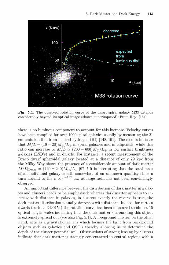
5 Dark Matter and Dark Energy 143
Fig. 5.1. The observed rotation curve of the dwarf spiral galaxy M33 extendsconsiderably beyond its optical image (shown superimposed); From Roy [164].
there is no luminous component to account for this increase. Velocity curveshave been compiled for over 1000 spiral galaxies usually by measuring the 21cm emission line from neutral hydrogen (HI) [148, 191]. The results indicatethat M/L = (10 − 20)M/L in spiral galaxies and in ellipticals, while thisratio can increase to M/L (200 − 600)M/L in low surface brightnessgalaxies (LSB’s) and in dwarfs. For instance, a recent measurement of theDraco dwarf spheroidal galaxy located at a distance of only 79 kpc fromthe Milky Way shows the presence of a considerable amount of dark matterM/L|Draco = (440 ± 240)M/L [97] ! It is interesting that the total massof an individual galaxy is still somewhat of an unknown quantity since aturn around to the v ∝ r−1/2 law at large radii has not been convincinglyobserved.
An important difference between the distribution of dark matter in galax-ies and clusters needs to be emphasised: whereas dark matter appears to in-crease with distance in galaxies, in clusters exactly the reverse is true, thedark matter distribution actually decreases with distance. Indeed, for certaindwarfs (such as DD0154) the rotation curve has been measured to almost 15optical length scales indicating that the dark matter surrounding this objectis extremely spread out (see also Fig. 5.1). A foreground cluster, on the otherhand, acts as a gravitational lens which focuses the light from backgroundobjects such as galaxies and QSO’s thereby allowing us to determine thedepth of the cluster potential well. Observations of strong lensing by clustersindicate that dark matter is strongly concentrated in central regions with a

144 Varun Sahni
projected mass of (1013 − 1014)M being contained within (0.2 - 0.3) Mpcof the central region. As we shall see later, this observation may prove tobe problematic for alternatives to the dark matter hypothesis such as theModified Newtonian Dynamics (MOND) approach of Milgrom [122].
As discussed earlier, the fact that only 4% of the cosmic density is bary-onic suggests that the dark matter which we are observing could well be non-baryonic in origin. The need for non-baryonic forms of dark matter gets indi-rect support from the fact that baryonic models find it difficult to grow struc-ture from small initial conditions and hence to reconcile the existence of a welldeveloped cosmic web of filaments, sheets and clusters at the present epochwith the exceedingly small amplitude of density perturbations (δρ/ρ ∼ 10−5
at z 1, 100) inferred from COBE measurements and more recent CMBexperiments. Indeed, it is well known that, if the effects of pressure are ig-nored, linearized density perturbations in a spatially flat matter dominateduniverse grow at the rate δ ∝ t2/3 ∝ (1 + z)−1, where 1 + z = a0/a(t) is thecosmological redshift. (Contrast this relatively slow growth rate with the ex-ponential ‘Jeans instability’ of a static matter distribution δ ∝ exp
√4πGρt.)
In a baryonic universe, the large radiation pressure (caused by Thompsonscattering of CMB photons off electrons) ensures that density perturbationsin the baryonic component can begin growing only after hydrogen recombinesat z 1, 100 at which point of time baryons and radiation decouple. Requir-ing δ > 1 today implies δ > 10−3 at recombination, which contradicts CMBobservations by over an order of magnitude ! In non-baryonic models on theother hand, the absence of any significant coupling between dark matter andradiation allows structure to grow much earlier, significantly before hydrogenin the universe has recombined. After recombination baryons simply fall intothe potential wells created for them by the dominant non-baryonic compo-nent. As a result a universe with a substantial non-baryonic component cangive rise to the structure which we see today from smaller initial fluctuations.
The growth of structure via gravitational instability depends both uponthe nature of primordial perturbations (adiabatic/isocurvature) and uponwhether the dark matter species is hot or cold. The issue of density pertur-bations has been discussed in considerable detail by R. Durrer in her contri-bution to this volume and I shall not touch upon this important topic anyfurther. Let me instead say a few words about hot and cold dark matter. Non-baryonic Hot Dark Matter (HDM) particles are assumed to have decoupledfrom the rest of matter/radiation when they were relativistic and so have avery large velocity dispersion (hence called ‘hot’). Cold Dark Matter (CDM)particles, on the other hand, have a very small velocity dispersion and de-couple from the rest of matter/radiation when they are non-relativistic. Thefree-streaming (collisionless phase mixing) of non-baryonic particles as theytravel from high density to low density regions (and vice versa) introducesan important length scale called the ‘free-streaming distance’ λfs – which isthe mean distance travelled by a relativistic particle species until its momen-tum becomes non-relativistic. In both HDM and CDM the processed final

5 Dark Matter and Dark Energy 145
spectrum of density perturbations differs from its initial form. In the caseof HDM this difference arises because fluctuations on scales smaller than λfsare wiped out due to free streaming with the result that the processed finalspectrum has a well defined cutoff on scales smaller than λ ∼ λfs. Perhaps thebest example of HDM is provided by a light neutrino of mass about 30 eV. Inthis case λfs 41(30eV/mν) Mpc with the result that large proto-pancakeshaving masses comparable to those of rich clusters of galaxies M ∼ 1015Mare the first objects to form in HDM. Smaller objects (galaxies) are formed bythe fragmentation of the proto-pancake. This top-down scenario for structureformation was originally suggested by Zeldovich and coworkers in connectionwith adiabatic baryonic models and subsequently applied to HDM. It hassince fallen out of favour mainly due to the strong observational constraintson the mass of the neutrino
∑νimνi
< 0.7 eV and on the relic neutrino den-sity 10−3 <∼ Ωνh
2 <∼ 10−1 [61, 193, 63, 123]. It also faces considerable difficultyin forming structure sufficiently early to explain the existence of galaxies andQSO’s at high redshifts.
In contrast to HDM, constituents of CDM have a much smaller free-streaming distance. Because of this small scales are the first to go non-linearand gravitational clustering proceeds in a bottom up fashion in this scenario.A key quantity defining gravitational clustering is the power spectrum ofdensity perturbations P (k) ≡ |δk|2, which is related to the mean squaredensity fluctuation via
⟨(δρ
ρ
)2⟩= 4π
∫ ∞
0P (k)k2dk . (5.6)
Inflationary models predict Pi(k) ∝ kn, n 1, at an early epoch. As theuniverse expands the power spectrum gets modified. The ‘processed’ finalspectrum depends upon the nature of dark matter, the epoch of matter-radiation equality and other cosmological quantities. The final and initialspectra are related through a transfer function
Pf (k) = Pi(k) × T 2(k) . (5.7)
CDM-type spectra have the following approximate form of the transfer func-tion [165, 194, 166]
T (k) =(
1 +Ak2
log (1 +Bk)
)−1
. (5.8)
Equations (5.7) and (5.8) illustrate the ‘turn around’ of the power spectrumfrom its primordial scale invariant form P (k) ∝ k on the largest scales toP (k) ∝ k−3 log2 k on small scales. (The precise location of the turn-aroundand the amplitude of P (k) depend upon specific details of the cosmologicalmodel, see for instance [16].)
The ‘standard’ cold dark matter (SCDM) paradigm, which assumed thatΩCDM = 1, was introduced during the early 1980’s at roughly the same time

146 Varun Sahni
when HDM was perceived to be in trouble (see [101, 96, 50, 166] for referencesto earlier work on this subject). Although SCDM was very successful in ex-plaining a host of observational details, it was clear already a decade ago, thatthe processed power spectrum of SCDM lacked sufficient power on large scalesand so fell short of explaining the angular two point correlation function forgalaxies on scales ∼ 50 Mpc [60]. The relevant cosmological quantity in thiscase is the shape of the power spectrum of density perturbations, which forCDM-like models, can be characterised by the ‘shape parameter’ Γ = Ωmh.SCDM models with Ωm = 1 and the HST-determined value h 0.7 predictΓ 0.5 which is much larger than the observed value Γ = 0.207 ± 0.030inferred from observations of galaxy clustering in the sloan digital sky survey(SDSS) [154]. A modification of SCDM called LCDM assumes that, in addi-tion to CDM the universe consists of a smoothly distributed component calleda cosmological constant or a Lambda-term. LCDM models with h 0.7 andΩm = 0.3 predict a smaller value for the shape parameter, Γ 0.2, and theresulting amplitude and shape of the power spectrum is in excellent agree-ment with several different sets of observations as demonstrated in Fig. 5.2.
From (5.6), (5.7) and (5.8) we find that on small scales, the contributionto the rms density fluctuation from a given logarithmic interval in k is
(δρ
ρ
)2
k
∼ k3Pf (k) ∝ log2 k , (5.9)
which illustrates the fact that, although the smallest scales are the first to gonon-linear, there is significant power to drive gravitational instability rapidlyto larger scales in this model. Indeed, detailed N-body simulations of largescale structure show that filaments defining the cosmic web first form on thesmallest scales. The scale-length characterizing the cosmic web grows as theuniverse expands, until at the present epoch the cosmic web consists of afully developed supercluster-void network with a scale-length of several tensof Megaparsec [181, 183, 119, 206].
Promising candidates for cold dark matter include a (100 − 1000) GeVparticle called a neutralino. The neutralino is a weakly interacting massiveparticle (WIMP). As its name suggests it is neutral and is a fermionic partnerto the gauge and Higgs bosons (usually called the ‘bino, wino and higgsino’).It is believed that the lightest supersymmetric particle will be stable dueto R-parity which makes the neutralino an excellent candidate for cold darkmatter (see [163, 89] for reviews of particle dark matter). A radically differentparticle candidate for cold dark matter is an ultra-light pseudo-Goldstone bo-son called an axion with a mass of onlyma ∼ 10−5±1 eV. Although ultralight,the axion is ‘cold’ because it was created as a zero-momentum condensate.Its existence is a by-product of an attempt to resolve QCD of what is com-monly called the ‘strong CP problem’ which arises because non-perturbativeeffects in QCD give rise to an electric dipole moment for the neutron, inmarked contrast with observations [101]. Other candidates for non-baryonic
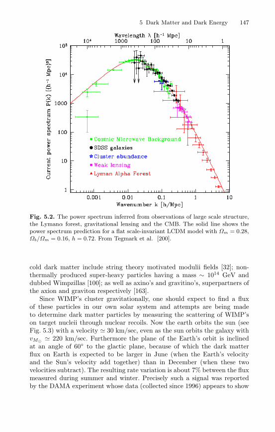
5 Dark Matter and Dark Energy 147
Fig. 5.2. The power spectrum inferred from observations of large scale structure,the Lymanα forest, gravitational lensing and the CMB. The solid line shows thepower spectrum prediction for a flat scale-invariant LCDM model with Ωm = 0.28,Ωb/Ωm = 0.16, h = 0.72. From Tegmark et al. [200].
cold dark matter include string theory motivated modulii fields [32]; non-thermally produced super-heavy particles having a mass ∼ 1014 GeV anddubbed Wimpzillas [100]; as well as axino’s and gravitino’s, superpartners ofthe axion and graviton respectively [163].
Since WIMP’s cluster gravitationally, one should expect to find a fluxof these particles in our own solar system and attempts are being madeto determine dark matter particles by measuring the scattering of WIMP’son target nucleii through nuclear recoils. Now the earth orbits the sun (seeFig. 5.3) with a velocity 30 km/sec, even as the sun orbits the galaxy withvM 220 km/sec. Furthermore the plane of the Earth’s orbit is inclinedat an angle of 60 to the glactic plane, because of which the dark matterflux on Earth is expected to be larger in June (when the Earth’s velocityand the Sun’s velocity add together) than in December (when these twovelocities subtract). The resulting rate variation is about 7% between the fluxmeasured during summer and winter. Precisely such a signal was reportedby the DAMA experiment whose data (collected since 1996) appears to show
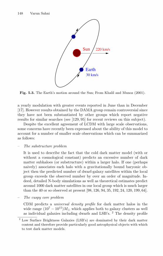
148 Varun Sahni
220 km/sSun
Earth 30 km/s
Fig. 5.3. The Earth’s motion around the Sun; From Khalil and Munoz (2001).
a yearly modulation with greater events reported in June than in December[17]. However results obtained by the DAMA group remain controversial sincethey have not been substantiated by other groups which report negativeresults for similar searches (see [129, 95] for recent reviews on this subject).
Despite the excellent agreement of LCDM with large scale observations,some concerns have recently been expressed about the ability of this model toaccount for a number of smaller scale observations which can be summarizedas follows:
– The substructure problem
It is used to describe the fact that the cold dark matter model (with orwithout a cosmological constant) predicts an excessive number of darkmatter subhaloes (or substructure) within a larger halo. If one (perhapsnaively) associates each halo with a gravitationally bound baryonic ob-ject then the predicted number of dwarf-galaxy satellites within the localgroup exceeds the observed number by over an order of magnitude. In-deed, detailed N-body simulations as well as theoretical estimates predictaround 1000 dark matter satellites in our local group which is much largerthan the 40 or so observed at present [98, 126, 94, 35, 192, 24, 120, 199, 64].
– The cuspy core problem
CDM predicts a universal density profile for dark matter halos in thewide range (107 − 1015)M which applies both to galaxy clusters as wellas individual galaxies including dwarfs and LSB’s. 2 The density profile
2 Low Surface Brightness Galaxies (LSB’s) are dominated by their dark mattercontent and therefore provide particularly good astrophysical objects with whichto test dark matter models.
5 Dark Matter and Dark Energy 149
originally suggested by Navarro, Frenk and White [133] is
ρ(r) = ρ0 (rs/r)[1 +(r
rs
)]−2
, (5.10)
which gives ρ ∝ r−1 for r rs and ρ ∝ r−3 for r rs, where rs is thescale radius and ρ0 is the characteristic halo density. (Other groups usinghigher resolution computations found somewhat steeper density profilesat small radii, such as ρ ∝ r−1.5 [127, 87].)The cuspy core problem refers to the apparent contradiction between N-body experiments, which show that the density profile in CDM halos hasa 1/r (or steeper) density cusp at the center, and observations, whichappear to favour significantly shallower density cores in galaxy clusters aswell as in individual dwarf and LSB galaxies (see [69, 36, 28, 37, 155, 199,103, 162, 179, 109] for detailed discussions of this issue).
Although disconcerting, given the very considerable success of LCDMin explaining gravitational clustering on large scales, it may at this pointbe premature to condemn this model on the basis of small scale observa-tions alone. It could be that the difficulties alluded to above are a result ofan oversimplification of the complex physical processes involved and that amore careful analysis of the baryonic physics on small scales including thehydrodynamical effects of star formation and supernova feedback needs to beundertaken. For instance both dwarfs and LSB’s have very shallow potentialwells, a strong burst of star formation and supernova activity may thereforeempty dark matter halos of their baryonic content resulting in a large num-ber of ‘failed galaxies’ and providing a possible resolution to the ‘satellitecatastrophe’. (The failed galaxies will act as gravitational lenses and shouldtherefore be detectable through careful observations.) Other explanations in-clude the effects of tidal stripping recently discussed in [103]. Likewise issuesinvolving beam smearing, the influence of bars and the interaction of baryonsand dark matter in the central regions of galaxies and clusters could be in-tricately linked with the central cusp issue and must be better understood ifone wishes to seriously test the CDM hypothesis on small scales.
In concluding this discussion on dark matter I would like to briefly men-tion Modified Newtonian Dynamics (MOND) which, in some circles, is re-garded as an alternative to the dark matter hypothesis. As the name suggests,MOND is a modification of Newtonian physics which proposes to explain theflat rotation curves of galaxies without invoking any assumptions about darkmatter. Briefly, MOND assumes that Newtons law of inertia (F = ma) ismodified at sufficiently low accelerations (a < a0) to
F = maµ(a/a0) , (5.11)
where µ(x) = x when x 1 and µ(x) = 1 when x 1 [122, 180]. It is easyto see that this results in the modification of the conventional formula for
150 Varun Sahni
gravitational acceleration F = mgN, resulting in the following relation be-tween the true acceleration and the Newtonian value: a =
√gNa0. For a body
orbiting a point mass M , gN = GM/r2. Since the centripetal accelerationa = v2/r now equals the true acceleration a, one gets
v4 = GMa0 , (5.12)
i.e. for sufficiently low values of the acceleration the rotation curve of anisolated body of mass M does not depend upon the radial distance r atwhich the velocity is measured, in other words not only does this theory pre-dict flat rotation curves it also suggests that the individual halo associatedwith a galaxy is infinite in extent ! (This latter prediction may be a prob-lem for MOND since recent galaxy-galaxy lensing results [82] suggest thatgalaxy halo’s may have a maximum extent of about 0.5 Mpc.) The value of a0needed to explain observations is a0 ∼ 10−8cm/s2 which is of the same orderas cH0 ! This has led supporters of this hypothesis to conjecture that MONDmay reflect “the effect of cosmology on local particle dynamics” [180]. Al-though MOND gives results which are in good agreement with observationsof individual galaxies, it is not clear whether it is as successful for explainingclusters for which strong gravitational lensing indicates a larger mass con-centration at cluster centers than accounted for by MOND [180, 52]. Anotherdifficulty with MOND is that it is problematic to embed this theory within amore comprehensive relativistic theory of gravity and hence, at present, it isnot clear what predictions a MOND-type theory may make for gravitationallensing and other curved space-time effects. For some recent developments inthis direction see [23].
To summarise, current observations make a strong case for clustered, non-baryonic dark matter to account for as much as a third of the total matterdensity in the Universe Ωm 1/3. The remaining two-thirds is thought toreside in a relative smooth component having large negative pressure andcalled Dark Energy.
5.2 Dark Energy
5.2.1 The Cosmological Constant and Vacuum Energy
Type Ia supernovae, when treated as standardized candles, suggest that theexpansion of the universe is speeding up rather than slowing down. The casefor an accelerating universe also receives independent support from CMB andlarge scale structure studies. All three data sets can be simultaneously satifiedif one postulates that the dominant component of the universe is relativelysmooth, has a large negative pressure and ΩDE 2/3.
The simplest example of dark energy is a cosmological constant, intro-duced by Einstein in 1917. The Einstein equations, in the presence of thecosmological constant, aquire the form

5 Dark Matter and Dark Energy 151
Rik − 12gikR =
8πGc4Tik + λgik . (5.13)
Although Einstein originally introduced the cosmological constant (λ) intothe left hand side of his field equations, it has now become conventional tomove the λ-term to the RHS, treating it as an effective form of matter. Ina homogeneous and isotropic Friedmann-Robertson-Walker (FRW) universeconsisting of pressureless dust (dark matter) and λ, the Raychaudhury equa-tion, which follows from (5.13), takes the form
a = −4πG3aρm +
λ
3. (5.14)
Equation (5.14) can be rewritten in the form of a force law:
F = −GMR2 +
λ
3R, (R ≡ a) (5.15)
which demonstrates that the cosmological constant gives rise to a repulsiveforce whose value increases with distance. The repulsive nature of λ could beresponsible for the acceleration of the universe as demonstrated in (5.14).
Although introduced into physics in 1917, the physical basis for a cosmo-logical constant remained a bit of a mystery until the 1960’s, when it wasrealised that zero-point vacuum fluctuations must respect Lorenz invarianceand therefore have the form 〈Tik〉 = λgik [214]. As it turns out, the vacuumexpectation value of the energy momentum is divergent both for bosonic andfermionic fields, and this gives rise to what is known as ‘the cosmologicalconstant problem’. Indeed the effective cosmological constant generated byvacuum fluctuations is
λ
8πG= 〈T00〉vac ∝
∫ ∞
0
√k2 +m2k2dk , (5.16)
since the integral diverges as k4 one gets an infinite value for the vacuumenergy. Even if one chooses to ‘regularize’ 〈Tik〉 by imposing an ultravioletcutoff at the Planck scale, one is still left with an enormously large value forthe vacuum energy 〈T00〉vac c5/G2
∼∼ 1076GeV4 which is 123 orders ofmagnitude larger than the currently observed ρλ 10−47GeV4. A smallerultraviolet cut-off does not fare much better since a cutoff at the QCD scaleresults in Λ4
QCD ∼ 10−3GeV4, which is still forty orders of magnitude largerthan observed.
In the 1970’s the discovery of supersymmetry led to the hope that, sincebosons and fermions (of identical mass) contribute equally but with oppositesign to the vacuum expectation value of physical quantities, the cosmologicalconstant problem may be resolved by a judicious balance between bosonsand fermions in nature. However supersymmetry (if it exists) is broken atthe low temperatures prevailing in the universe today and on this accountone should expect the cosmological constant to vanish in the early universe,
152 Varun Sahni
but to reappear during late times when the temperature has dropped belowTSUSY. This is clearly an undesirable scenario and almost the very oppositeof what one is looking for, since, a large value of λ at an early time is usefulfrom the viewpoint of inflation, whereas a very small current value of λ is inagreement with observations [172, 171].
In the absence of a resolution to the cosmological constant problem the fol-lowing possibility connecting the vacuum energy with the SUSY and Planckscales may be worth exploring [172, 171]. The mass scale associated with thescale of supersymmetry breaking in some models, MSUSY ∼ 1 TeV, lies mid-way between the Planck scale and 10−3 eV. One could conjecture that thesmall observed value of the cosmological constant ρλ (10−3eV )4 is asso-ciated with the vacuum in a theory which had a fundamental mass scaleMX M2
SUSY/MPl, such that ρvac ∼M4X ∼ (10−3eV )4.
The cosmological constant is also relevant from the perspective of mod-els with spontaneous symmetry breaking [209]. Indeed, if one examines theLagrangian
L =12gij∂iφ∂jφ− V (φ)
V (φ) = V0 − 12µ2φ2 +
14λφ4, (5.17)
one notices that the symmetric state at φ = 0 is unstable and the systemsettles in the ground state φ = +σ or φ = −σ, where σ =
√µ2/λ, thereby
breaking the reflection symmetry φ ↔ −φ present in the Lagrangian. ForV0 = 0 this potential gives rise to a large negative cosmological constantλeff = V (φ = σ) = −µ4/4λ in the broken symmetry state. This embarrassingsituation can be avoided only if one chooses a value for V0 which almostexactly cancels λeff , namely V0 +µ4/4λ so that λeff/8πG = V0−µ4/4λ 10−47GeV 4.
The cosmological consequences of this rather ad-hoc ‘regularization’ ex-ercise are instructive. Unless the value of λeff lies in a very small window,the universe will be a very different place from the one we are used to. Forinstance a negative value of the λ-term λeff/8πG < −10−43GeV 4 will causethe universe to recollapse (the effect of λ is attractive now instead of beingrepulsive) less than a billion years after the big bang – a period which ismuch too short for galaxies to form and for life (as we know it) to emerge.On the other hand a large positive λeff/8πG > 10−43GeV4 makes the uni-verse accelerate much before the present epoch, thereby inhibiting structureformation and precluding the emergence of life.
The very small window in λ which allows life to emerge has led somecosmologists to propose anthropic arguments for the existence of a smallcosmological constant [20, 118, 76, 210]. One such possibility is the following“if our big bang is just one of many big bangs, with a wide range of vacuumenergies, then it is natural that some of these big bangs should have a vacuumenergy in the narrow range where galaxies can form, and of course it is just
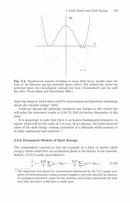
5 Dark Matter and Dark Energy 153
Fig. 5.4. Spontaneous symetry breaking in many field theory models takes theform of the Mexican top hat potential shown above. The dashed line shows thepotential before the cosmological constant has been ‘renormalized’ and the solidline after. (From Sahni and Starobinsky 2000.)
these big bangs in which there could be astronomers and physicists wonderingabout the vacuum energy” [210].
I will not discuss the anthropic argument any further in this review butwill point the interested reader to [118, 76, 210] for further discussion of thisissue.
It is important to note that there is no known fundamental symmetry innature which will set the value of λ to zero. In its absence, the small observedvalue of the dark energy remains somewhat of a dilemma which remains tobe fully understood and resolved. 3
5.2.2 Dynamical Models of Dark Energy
The cosmological constant is but one example of a form of matter (darkenergy) which could drive an accelerated phase in the history of our universe.Indeed, (5.14) is easily generalised to
a
a= −4πG
3
∑
i
(ρi + 3pi) = −4πG3
∑
i
ρi(1 + 3wi) , (5.18)
3 The important role played by symmetries is illustrated by the U(1) gauge sym-metry of electrodynamics whose presence implies a zero rest mass for the photon.No analogous symmetry exists for the neutrino and recent experiments do indi-cate that neutrino’s could have a small mass.

154 Varun Sahni
where the summation is over all forms of matter present in the universe withequation of state wi = pi/ρi. Equation (5.18) together with its companionequation
H2 ≡(a
a
)2
=8πG
3
∑
i
ρi − k
a2(5.19)
completely describes the dynamics of a FRW universe (k/a2 is the Gaussiancurvature of space).
Clearly a universe consisting of only a single component will accelerate ifw < −1/3. Fluids satisfying ρ + 3p ≥ 0 or w ≥ −1/3 are said to satisfy the‘strong energy condition’ (SEC). We therefore find that, in order to acceler-ate, ‘dark energy’ must violate the SEC. Another condition which is usuallyassumed to be sacrosanct, but has recently been called into question is the‘weak energy condition’ (WEC) ρ + p ≥ 0 or w ≥ −1. Failure to satisfy theWEC can result in faster-than-exponential expansion for the universe and ina cosmic ‘Big Rip’, which we shall come to in a moment.
It is often more convenient to rewrite (5.18) in terms of the ‘decelerationparameter’
q = − a
aH2 =∑
i
(4πGρi
3H2 )(1 + 3wi) =(1 + 3wXΩX)
2, (5.20)
where Ωi = 8πGρi/3H2 and we have assumed a flat universe with Ωm+ΩX =1 (ΩX ≡ ΩDE). The condition for accelerated expansion (q < 0) is equivalentto
wX < − 13(1 −Ωm)
, (5.21)
which leads to
w < −13
for Ωm = 0 (5.22)
w < −12
for Ωm = 1/3 . (5.23)
Equation (5.19) can be used to develop an expression for the Hubbleparameter H ≡ a/a in terms of the cosmological redshift z = a0/a(t) − 1:
H(z) = H0
[Ωm(1 + z)3 +ΩX(1 + z)3(1+w)
]1/2, (5.24)
where H0 = H(z = 0) is the present value of the Hubble parameter, Ωm =8πGρ0m/3H2
0 , ΩX = 8πGρ0DE/3H20 , describe the dimensionless density of
matter and dark energy respectively, (w ≡ wDE), and we have made theassumption of a flat universe so that Ωm +ΩX = 1.
In LCDM cosmology w = −1, ΩΛ = λ/3H20 , and the expansion factor has
the elegant form [172]

5 Dark Matter and Dark Energy 155
a(t) ∝(
sinh32
√Λ
3ct
)2/3
, (5.25)
which smoothly interpolates between a matter dominated universe in the past
(a ∝ t2/3) and accelerated expansion in the future (a ∝ exp√
Λ3 t).
We are now in a position to appreciate the evidence for an acceleratinguniverse which originates in observations of the light flux from high redshifttype Ia supernovae. Type Ia supernovae are extremely bright objects, (MB −19.5) which makes them ideally suited for studying the properties of theuniverse at large distances.
The light flux received from a distant supernova is related to its absoluteluminosity L and its ‘luminosity distance’ dL through the relation
F =L
4πd2L. (5.26)
If one views this problem from within the Newtonian perspective then, sincethe geometry of space is Euclidean, dL =
√x2 + y2 + z2. In general relativity,
on the other hand, the geometry of space can be non-Euclidean, and theluminosity distance to an object located at redshift z will, in general, dependboth upon the geometry of space as well as the expansion history of theuniverse. Indeed, it can be shown that in a spatially flat and expanding FRWuniverse, the luminosity distance has the form
dL(z) = (1 + z)∫ z
0
dz′
H(z′). (5.27)
The luminosity distance is shown in Fig. 5.5 for a number of cosmologicalmodels with varying amounts of Ωm and ΩΛ. The limiting case Ωm = 1,ΩΛ = 0 corresponds to standard cold dark matter (SCDM) in which theuniverse decelerates as a weak power law a(t) ∝ t2/3. The other extremeexample ΩΛ = 1, Ωm = 0 describes the de Sitter universe (also known as
steady state cosmology) which accelerates at the steady rate a(t) ∝ exp√
Λ3 t.
From Fig. 5.5 we see that a supernova at redshift z = 3 will appear 9 timesbrighter in SCDM than it will in de Sitter space !
Systematic studies of type Ia supernovae have revealed that:
– Type Ia Sn are excellent stadardized candles. The dispersion in peak su-pernova luminosity is small: ∆m 0.3, and the corresponding change inintensity is about 25%. In addition the light curve of a type Ia supernovais correlated with its peak luminosity [149] to a precision of ∼ 7%, sothat brighter supernovae take longer to fade. (Type Ia Sn take roughly20 days to rise from relative obscurity to maximum light.) This allowsus to ‘standardize’ supernova light curves thereby reducing the scatterin their luminosities to ∼ 12% which turns type Ia supernovae into verygood standard candles.
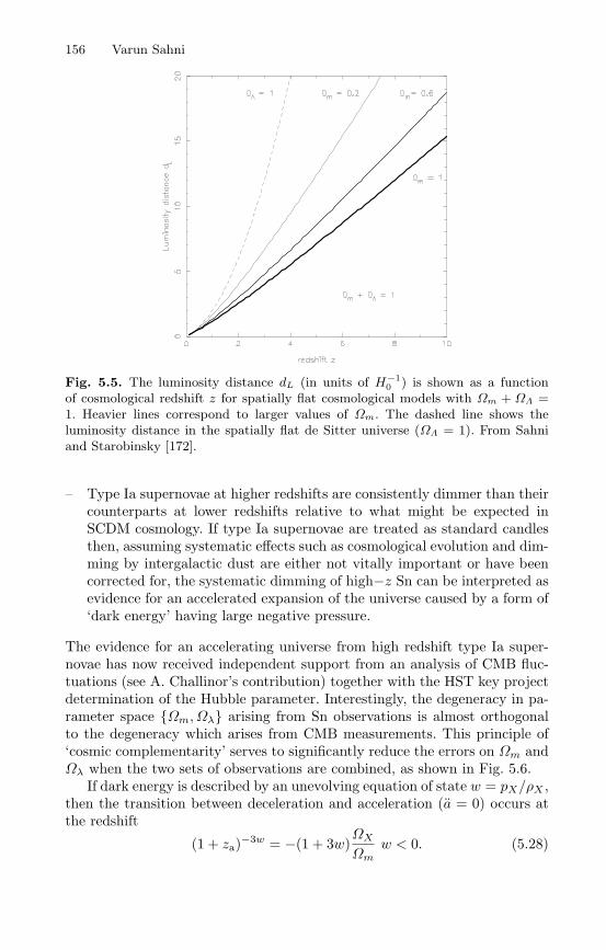
156 Varun Sahni
Fig. 5.5. The luminosity distance dL (in units of H−10 ) is shown as a function
of cosmological redshift z for spatially flat cosmological models with Ωm + ΩΛ =1. Heavier lines correspond to larger values of Ωm. The dashed line shows theluminosity distance in the spatially flat de Sitter universe (ΩΛ = 1). From Sahniand Starobinsky [172].
– Type Ia supernovae at higher redshifts are consistently dimmer than theircounterparts at lower redshifts relative to what might be expected inSCDM cosmology. If type Ia supernovae are treated as standard candlesthen, assuming systematic effects such as cosmological evolution and dim-ming by intergalactic dust are either not vitally important or have beencorrected for, the systematic dimming of high−z Sn can be interpreted asevidence for an accelerated expansion of the universe caused by a form of‘dark energy’ having large negative pressure.
The evidence for an accelerating universe from high redshift type Ia super-novae has now received independent support from an analysis of CMB fluc-tuations (see A. Challinor’s contribution) together with the HST key projectdetermination of the Hubble parameter. Interestingly, the degeneracy in pa-rameter space Ωm, Ωλ arising from Sn observations is almost orthogonalto the degeneracy which arises from CMB measurements. This principle of‘cosmic complementarity’ serves to significantly reduce the errors on Ωm andΩλ when the two sets of observations are combined, as shown in Fig. 5.6.
If dark energy is described by an unevolving equation of state w = pX/ρX ,then the transition between deceleration and acceleration (a = 0) occurs atthe redshift
(1 + za)−3w = −(1 + 3w)ΩX
Ωmw < 0. (5.28)

5 Dark Matter and Dark Energy 157
Fig. 5.6. Constraints on the density of dark matter Ωm and dark energy in the formof a cosmological constant Ωλ, determined using WMAP (upper left), WMAP +other CMB experiments (WMAPext; upper right), WMAPext + HST key projectdata (lower left) and WMAPext + HST + supernova data (lower right); fromSpergel et al (2003).
Another important redshift describes the epoch when the densities in darkmatter and dark energy are equal
(1 + zeq)3w =(Ωm
ΩX
). (5.29)
Substituting ΩΛ = 0.7, Ωm = 0.3 we find za 0.73, zeq 0.37 for LCDM.The fact that the acceleration of the universe is a fairly recent phenomenon il-lustrates the ‘cosmic coincidence’ puzzle according to which we appear to liveduring a special epoch when the densities in dark energy and in dark matterare almost equal. A recent origin for the acceleration epoch is supported bysupernova observations which suggest a decelerating universe at z >∼ 0.5 [160].It is important to note that dark energy models with an unevolving equa-tion of state need to have their initial conditions properly ‘tuned’ in order todominate the universe at precisely the present epoch. This problem is mostacute for the cosmological constant. Since the cosmological constant does notevolve while both matter and radiation evolve rapidly (ρm ∝ a−3, ρr ∝ a−4),it follows that the small current value ρΛ = λ/8πG 10−47 GeV4 impliesρΛ/ρr 10−123 at the Planck time (when the temperature of the universewas T ∼ 1019 GeV), or ρΛ/ρr 10−55 at the time of the electroweak phasetransition (T ∼ 100 GeV). Thus an extreme fine-tuning of initial conditionsis required in order to ensure that ρΛ/ρm ∼ 1 today !
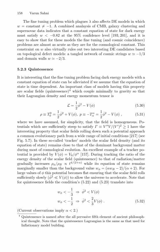
158 Varun Sahni
The fine tuning problem which plagues λ also affects DE models in whichw = constant = −1. A combined analaysis of CMB, galaxy clustering andsupernovae data indicates that a constant equation of state for dark energymust satisfy w < −0.82 at the 95% confidence level [193, 201], and it iseasy to show that for these models the fine tuning (and cosmic coincidence)problems are almost as acute as they are for the cosmological constant. Thisconstraint on w also virtually rules out two interesting DE candidates basedon topological defect models: a tangled network of cosmic strings w −1/3and domain walls w −2/3.
5.2.3 Quintessence
It is interesting that the fine tuning problem facing dark energy models with aconstant equation of state can be alleviated if we assume that the equation ofstate is time dependent. An important class of models having this propertyare scalar fields (quintessence)4 which couple minimally to gravity so thattheir Lagrangian density and energy momentum tensor is
L =12φ2 − V (φ) (5.30)
ρ ≡ T 00 =
12φ2 + V (φ), p ≡ −Tα
α =12φ2 − V (φ) , (5.31)
where we have assumed, for simplicity, that the field is homogeneous. Po-tentials which are sufficiently steep to satisfy Γ ≡ V ′′V/(V ′)2 ≥ 1 have theinteresting property that scalar fields rolling down such a potential approacha common evolutionary path from a wide range of initial conditions [217] (seeFig. 5.7). In these so-called ‘tracker’ models the scalar field density (and itsequation of state) remains close to that of the dominant background matterduring most of cosmological evolution. An excellent example of a tracker po-tential is provided by V (φ) = V0/φ
α [157]. During tracking the ratio of theenergy density of the scalar field (quintessence) to that of radiation/mattergradually increases ρφ/ρB ∝ t4/(2+α) while its equation of state remainsmarginally smaller than the background value wφ = (αwB − 2)/(α+ 2). Forlarge values of φ this potential becomes flat ensuring that the scalar field rollssufficiently slowly (φ2 V (φ)) to allow the universe to accelerate. Note thatfor quintessence fields the condition’s (5.22) and (5.23) translate into
wφ < −13
⇒ φ2 < V (φ)
wφ < −12
⇒ φ2 <23V (φ) . (5.32)
(Current observations imply α < 2.)4 Quintessence is named after the all pervasive fifth element of ancient philosoph-
ical thought. Note that the quintessence Lagrangian is the same as that used forInflationary model building.
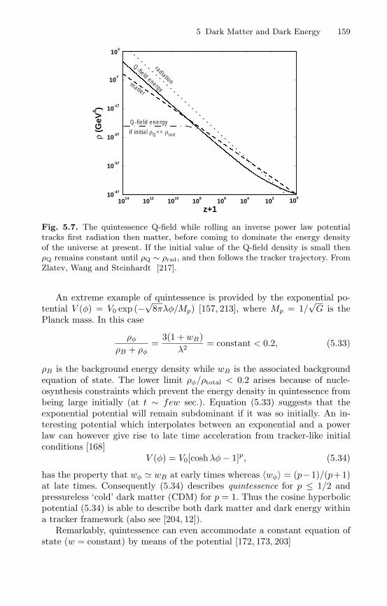
5 Dark Matter and Dark Energy 159
1014
1012
1010
108
106
104
102 10
0
z+1
10-47
10-37
10-27
10-17
10-7
103
ρ (G
eV4 )
radiationmatter
Q-field energy
Q-field energy
if initial ρQ<< ρrad
Fig. 5.7. The quintessence Q-field while rolling an inverse power law potentialtracks first radiation then matter, before coming to dominate the energy densityof the universe at present. If the initial value of the Q-field density is small thenρQ remains constant until ρQ ∼ ρrad, and then follows the tracker trajectory. FromZlatev, Wang and Steinhardt [217].
An extreme example of quintessence is provided by the exponential po-tential V (φ) = V0 exp (−√
8πλφ/Mp) [157, 213], where Mp = 1/√G is the
Planck mass. In this case
ρφ
ρB + ρφ=
3(1 + wB)λ2 = constant < 0.2, (5.33)
ρB is the background energy density while wB is the associated backgroundequation of state. The lower limit ρφ/ρtotal < 0.2 arises because of nucle-osynthesis constraints which prevent the energy density in quintessence frombeing large initially (at t ∼ few sec.). Equation (5.33) suggests that theexponential potential will remain subdominant if it was so initially. An in-teresting potential which interpolates between an exponential and a powerlaw can however give rise to late time acceleration from tracker-like initialconditions [168]
V (φ) = V0[coshλφ− 1]p, (5.34)
has the property that wφ wB at early times whereas 〈wφ〉 = (p−1)/(p+1)at late times. Consequently (5.34) describes quintessence for p ≤ 1/2 andpressureless ‘cold’ dark matter (CDM) for p = 1. Thus the cosine hyperbolicpotential (5.34) is able to describe both dark matter and dark energy withina tracker framework (also see [204, 12]).
Remarkably, quintessence can even accommodate a constant equation ofstate (w = constant) by means of the potential [172, 173, 203]

160 Varun Sahni
Table 5.1.
Quintessence Potential Reference
V0 exp (−λφ) Ratra and Peebles (1988), Wetterich (1988),Ferreira and Joyce (1998)
m2φ2, λφ4 Frieman et al (1995)
V0/φα, α > 0 Ratra and Peebles (1988)
V0 exp (λφ2)/φα Brax and Martin (1999, 2000)
V0(coshλφ− 1)p Sahni and Wang (2000)
V0 sinh−α (λφ) Sahni and Starobinsky (2000),Urena-Lopez & Matos (2000)
V0(eακφ + eβκφ) Barreiro, Copeland and Nunes ( 2000)
V0(expMp/φ− 1) Zlatev, Wang and Steinhardt (1999)
V0[(φ−B)α +A]e−λφ Albrecht and Skordis (2000)
V (φ) ∝ sinh2(1+w)
w (Cφ+D) , (5.35)
with suitably chosen values of C,D.Quintessence models can be divided into two categories: models which
roll to large values of φ/mP >∼ 1 and models for which φ/mP 1 at thepresent epoch. An important concern for the former is the effect of quantumcorrections which, if large, could alter the shape of the quintessence potential[102, 33, 59, 182]. An important related issue is that the coupling betweenstandard model fields and quintessence must be small in order to have evadeddetection. Moreover even small couplings between quintessence and standardmodel fields can give rise to interesting changes in cosmology as shown in[6, 114].
I would like to end this section by mentioning that, due to the short-age of time I have not been able to cover all of the DE models suggested inthe literature (a number that is growing rapidly !) For this reason this re-view will not discuss DE due to vacuum polarization[167, 141], k-essence [13],Cardassian expansion [73], Quasi-Steady State Cosmology [132], scalar-tensormodels [5, 26, 45, 145, 205, 146, 161, 29, 147]. For other interesting approachessee [15, 83, 84, 62, 137, 80, 104, 105, 125, 187, 215]. A partial list of some pop-ular quintessence models is given in Table 1, and the reader is also referredto the dark energy reviews in [172, 41, 143, 171, 140].
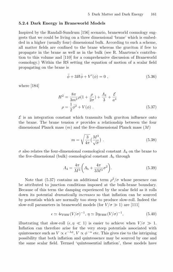
5 Dark Matter and Dark Energy 161
5.2.4 Dark Energy in Braneworld Models
Inspired by the Randall-Sundrum [156] scenario, braneworld cosmology sug-gests that we could be living on a three dimensional ‘brane’ which is embed-ded in a higher (usually four) dimensional bulk. According to such a scheme,all matter fields are confined to the brane whereas the graviton if free topropagate in the brane as well as in the bulk (see R. Maartens’s contribu-tion to this volume and [110] for a comprehensive discussion of Braneworldcosmology.) Within the RS setting the equation of motion of a scalar fieldpropagating on the brane is
φ+ 3Hφ+ V ′(φ) = 0 , (5.36)
where [184]
H2 =8π
3m2 ρ(1 +ρ
2σ) +
Λ4
3+
Ea4
ρ =12φ2 + V (φ) . (5.37)
E is an integration constant which transmits bulk graviton influence ontothe brane. The brane tension σ provides a relationship between the fourdimensional Planck mass (m) and the five-dimensional Planck mass (M)
m =
√34π(M3√σ
). (5.38)
σ also relates the four-dimensional cosmological constant Λ4 on the brane tothe five-dimensional (bulk) cosmological constant Λb through
Λ4 =4πM3
(Λb +
4π3M3σ
2). (5.39)
Note that (5.37) contains an additional term ρ2/σ whose presence canbe attributed to junction conditions imposed at the bulk-brane boundary.Because of this term the damping experienced by the scalar field as it rollsdown its potential dramatically increases so that inflation can be sourcedby potentials which are normally too steep to produce slow-roll. Indeed theslow-roll parameters in braneworld models (for V/σ 1) are [111]
ε 4εFRW(V/σ)−1, η 2ηFRW(V/σ)−1, (5.40)
illustrating that slow-roll (ε, η 1) is easier to achieve when V/σ 1.Inflation can therefore arise for the very steep potentials associated withquintessence such as V ∝ e−λφ, V ∝ φ−α etc. This gives rise to the intriguingpossibility that both inflation and quintessence may be sourced by one andthe same scalar field. Termed ‘quintessential inflation’, these models have
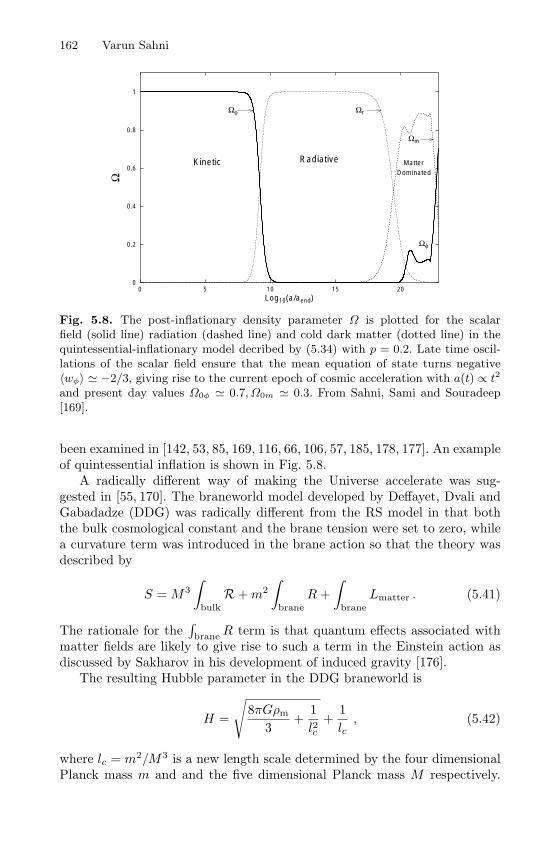
162 Varun Sahni
0
0.2
0.4
0.6
0.8
1
0 5 10 15 20
Ω
Log10(a/aend)
Ωφ Ωr
Ωm
Ωφ
Kinetic Radiative MatterDominated
Fig. 5.8. The post-inflationary density parameter Ω is plotted for the scalarfield (solid line) radiation (dashed line) and cold dark matter (dotted line) in thequintessential-inflationary model decribed by (5.34) with p = 0.2. Late time oscil-lations of the scalar field ensure that the mean equation of state turns negative〈wφ〉 −2/3, giving rise to the current epoch of cosmic acceleration with a(t) ∝ t2
and present day values Ω0φ 0.7, Ω0m 0.3. From Sahni, Sami and Souradeep[169].
been examined in [142, 53, 85, 169, 116, 66, 106, 57, 185, 178, 177]. An exampleof quintessential inflation is shown in Fig. 5.8.
A radically different way of making the Universe accelerate was sug-gested in [55, 170]. The braneworld model developed by Deffayet, Dvali andGabadadze (DDG) was radically different from the RS model in that boththe bulk cosmological constant and the brane tension were set to zero, whilea curvature term was introduced in the brane action so that the theory wasdescribed by
S =M3∫
bulkR +m2
∫
braneR+
∫
braneLmatter . (5.41)
The rationale for the∫braneR term is that quantum effects associated with
matter fields are likely to give rise to such a term in the Einstein action asdiscussed by Sakharov in his development of induced gravity [176].
The resulting Hubble parameter in the DDG braneworld is
H =
√8πGρm
3+
1l2c
+1lc, (5.42)
where lc = m2/M3 is a new length scale determined by the four dimensionalPlanck mass m and and the five dimensional Planck mass M respectively.

5 Dark Matter and Dark Energy 163
An important property of this model is that the acceleration of the universeis not caused by the presence of any ‘dark energy’. Instead, since gravitybecomes five dimensional on length scales R > lc = 2H−1
0 (1 − Ωm)−1, onefinds that the expansion of the universe is modified during late times insteadof early times as in the RS model.
A more general class of braneworld models which includes RS cosmologyand the DDG brane as subclasses was developed in [51, 189] and is describedby the action
S =M3∫
bulk(R − 2Λb) +
∫
brane
(m2R− 2σ
)+∫
braneLmatter . (5.43)
For σ = λb = 0 (5.43) reduces to the action describing the DDG model,whereas for m = 0 it describes the Randall-Sundrum model.
As demonstrated by Sahni and Shtanov [170] the braneworld which followsfrom the action (5.43) describes an accelerating universe at late times withthe Hubble parameter
H2(z)H2
0= Ωm(1+z)3 +Ωσ + 2Ωl ∓
2√Ωl
√Ωm(1+z)3 +Ωσ +Ωl +Ωλb , (5.44)
where
Ωl =1
l2cH20, Ωm =
ρ0m
3m2H20, Ωσ =
σ
3m2H20, Ωλb = − λb
6H20. (5.45)
(The ∓ signs refer to the two different ways in which the brane can be embed-ded in the bulk, both signs give rise to interesting cosmology [170].) As in theDDG model lc ∼ H−1
0 if M ∼ 100 MeV. On short length scales r lc andat early times, one recovers general relativity, whereas on large length scalesr lc and at late times brane-related effects begin to play an importantrole. Indeed by setting M = 0 (Ωl = 0) (5.44) reduces to the LCDM model
H2(z)H2
0= Ωm(1+z)3 +Ωσ , (5.46)
whereas for σ = λb = 0 (5.44) reduces to the DDG braneworld. An importantfeature of the braneworld (5.44) is that it can lead to an effective equationof state of dark energy weff ≤ −1. This is easy to see from the expression forthe current value of the effective equation of state [170]
w0 =2q0 − 1
3 (1 −Ωm)= −1 ± Ωm
1 −Ωm
√Ω
Ωm +Ωσ +Ω +ΩΛb
, (5.47)
we find that w0 < −1 when we take the lower sign in (5.47), which corre-sponds to choosing one of two possible embeddings of this braneworld in thehigher dimensional bulk. (The second choice of embedding gives w0 > −1.)

164 Varun Sahni
It is also possible, in this model, for the acceleration of the universe tobe a transient phenomenon which ends once the universe returns to matterdominated expansion after the current accelerating phase. As discussed in[170] such a braneworld will not have an event horizon and may thereforehelp in reconciling an accelerating universe with the demands of string/M-theory. Other possibilities of obtaining dark energy from extra dimensionshave been discussed in [7, 144, 44, 150, 151, 117, 34, 138]. The possibility thatDE could arise due to modifications of gravitational physics has also beenexamined in [108, 40, 43, 58, 124, 135, 136].
5.2.5 Chaplygin Gas
A completely different route to dark energy is provided by the Chaplygin gas[92] which obeys the equation of state
pc = −A/ρc . (5.48)
The conservation equation dE = −pdV ⇒ d(ρa3) = −pd(a3) immediatelygives
ρc =
√
A+B
a6=√A+B(1 + z)6 , (5.49)
where B is a constant of integration. Thus the Chaplygin gas behaves likepressureless dust at early times and like a cosmological constant during verylate times.
The Hubble parameter for a universe containing cold dark matter and theChaplygin gas is given by
H(z) = H0
[
Ωm(1 + z)3 +Ωm
κ
√A
B+ (1 + z)6
]1/2
, (5.50)
where κ = ρ0m/√B and it is easy to see from (5.50) that
κ =ρ0m
ρc(z → ∞) . (5.51)
Thus, κ defines the ratio between CDM and the Chaplygin gas energy densi-ties at the commencement of the matter-dominated stage. It is easy to showthat
A = B
κ2(
1 −Ωm
Ωm
)2
− 1
. (5.52)
It is interesting that the Chaplygin gas can be derived from an underlyingLagrangian in two distinct ways:
– One can derive it from a quintessence Lagrangian (5.30) with the potential[92]
V (φ) =√A
2
(cosh 3φ+
1cosh 3φ
). (5.53)
5 Dark Matter and Dark Energy 165
– The Chaplygin gas can also be derived from the Born-Infeld form of theLagrangian density
L = −V0√
1 − φ,µφ,µ , (5.54)
where φ,µ ≡ ∂φ/∂xµ. For time-like φ,µ one can define a four velocity
uµ =φ,µ
√φ,αφ,α
, (5.55)
this leads to the standard form for the hydrodynamical energy-momentumtensor
Tµν = (ρ+ p)uµuν − pgµν , (5.56)
where [75]
ρ =V0√
1 − φ,µφ,µ, p = −V0
√1 − φ,µφ,µ , (5.57)
i.e. we have recovered (5.48) with A = V 20 .
The fact that the properties of the Chaplygin gas interpolate betweenthose of CDM and a λ-term led to the hope that the CG might provide aconceptual framework for a unified model of dark matter and dark energy. Itshould however be noted that in contrast to CDM and baryons, the soundvelocity in the Chaplygin gas vc =
√dpc/dρc =
√A/ρc quickly grows ∝ t2
during the matter-dominated regime and becomes of the order of the velocityof light at present (it approaches light velocity asymptotically in the distantfuture). Thus, when one examines classical inhomogeneities, the properties ofthe Chaplygin gas during the matter-dominated epoch appear to be ratherunusual and resemble those of hot dark matter rather than CDM, despite thefact that the Chaplygin gas formally carries negative pressure [2].
A ‘generalized Chaplygin gas’ has also been proposed for which p ∝−1/ρα. The equation of state in this case is
w(a) = − |w0|[|w0| + 1−|w0|
a3(1+α)
] , (5.58)
which interpolates between w = 0 at early times (a 1) and w = −1 at latetimes (a 1); w0 is the current equation of state at a = 1. (The constant αregulates the transition time in the equation of state.) WMAP, supernovaeand large scale sructure data have all been used to test Chaplygin gas models;see [27, 65, 78, 9, 14, 22, 115, 128, 56, 25].
5.2.6 Is Dark Energy a Phantom?
In an influential paper Caldwell [38] noticed that a very good fit to thesupernova-derived luminosity distance was provided by dark energy which
166 Varun Sahni
violated the weak energy condition so that w < −1. He called this Phantomdark energy.5 Indeed, a study of high-z Sn [99] finds that the DE equationof state has a 99% probability of being < −1 if no priors are placed onΩm ! When these Sn results are combined with CMB and 2dFGRS the 95%confidence limits on an unevolving equation of state are −1.61 < w < −0.78[99], which is consistent with estimates made by other groups [193, 201].
A universe filled with Phantom energy has some interesting but bizarreproperties.
– If teq marks the epoch when the densities in matter and phantom energyare equal then the expansion factor of a universe dominated by phantomenergy grows as
a(t) a (teq)[(1 + w)
t
teq− w]2/
3(1+w)
, w < −1 , (5.59)
and therefore diverges in a finite amount of cosmic time
a(t) → ∞ as t→ tBR =(
w
1 + w
)teq . (5.60)
By substituting w < −1 into (5.24) we immediately find that the Hubbleparameter also diverges as t → tBR, implying that an infinitely rapidexpansion rate for the universe has been reached in a finite time. Thedivergence of the Hubble parameter is associated with the divergence ofphantom density which grows without bound
ρ(t) ∝[(1 + w)
t
teq− w]−2
, (5.61)
and reaches a singular value in a finite interval of time ρ(t) → ∞, t→ tBR.Thus a universe dominated by Phantom energy culminates in a future cur-vature singularity (‘Big Rip’) at which the notion of a classical space-timebreaks down. (See also [196, 47, 38, 121, 39, 42, 71, 72, 186, 88, 10, 93].)
– The ultra-negative phantom equation of state suggests that the effectivevelocity of sound in the medium v =
√|dp/dρ| can become larger thanthe velocity of light in this model.
– Although a dynamical model of phantom energy can be constructed withthe ‘wrong’ sign of the kinetic term, see (5.31), such models are plaguedwith instabilities at the quantum level [49] which makes their existencesuspected.It should be pointed out that phantom is not the only way to get w < −1.A model with similar properties but sharing none of phantom’s patholo-gies is the braneworld model of [170, 1], which has weff < −1 today butdoes not run into a ‘Big Rip’ in the future.
5 Phantom takes its name from Part I of the Star Wars movie series – the PhantomMenace.
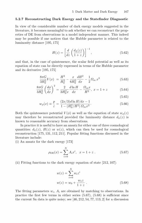
5 Dark Matter and Dark Energy 167
5.2.7 Reconstructing Dark Energy and the Statefinder Diagnostic
In view of the considerable number of dark energy models suggested in theliterature, it becomes meaningful to ask whether we can reconstruct the prop-erties of DE from observations in a model independent manner. This indeedmay be possible if one notices that the Hubble parameter is related to theluminosity distance [195, 175]
H(z) =[d
dz
(dL(z)1 + z
)]−1
, (5.62)
and that, in the case of quintessence, the scalar field potential as well as itsequation of state can be directly expressed in terms of the Hubble parameterand its derivative [195, 175]
8πG3H2
0V (x) =
H2
H20
− x
6H20
dH2
dx− 1
2Ωm x
3 (5.63)
8πG3H2
0
(dφ
dx
)2
=2
3H20x
d lnHdx
− Ωmx
H2 , x = 1 + z (5.64)
(5.65)
wφ(x) ≡ p
ε=
(2x/3)d lnH/dx− 11 − (H2
0/H2)Ωmx3 . (5.66)
Both the quintessence potential V (φ) as well as the equation of state wφ(z)may therefore be reconstructed provided the luminosity distance dL(z) isknown to reasonable accuracy from observations.
In practice it is useful to have an ansatz for either one of three cosmologicalquantities: dL(z), H(z) or w(z), which can then be used for cosmologicalreconstruction [175, 131, 112, 211]. Popular fitting functions discussed in theliterature include:(i) An ansatz for the dark energy [173]
ρDE(x) =N∑
i=0
Aixi, x = 1 + z . (5.67)
(ii) Fitting functions to the dark energy equation of state [212, 107]:
w(z) =N∑
i=0
wizi
w(z) = w0 +w1z
1 + z. (5.68)
The fitting parameters wi, Ai are obtained by matching to observations. Inpractice the first few terms in either series (5.67), (5.68) is sufficient sincethe current Sn data is quite noisy; see [46, 212, 54, 77, 113, 2] for a discussion
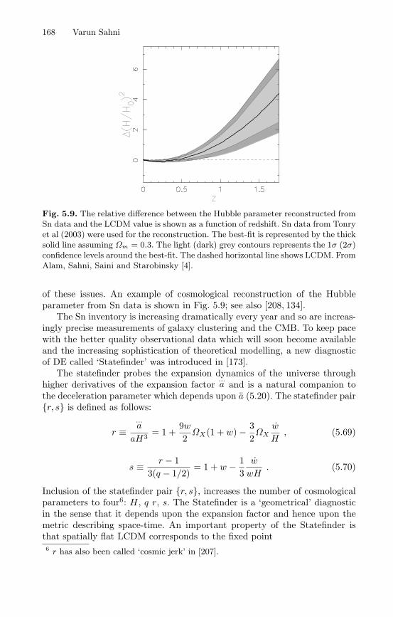
168 Varun Sahni
Fig. 5.9. The relative difference between the Hubble parameter reconstructed fromSn data and the LCDM value is shown as a function of redshift. Sn data from Tonryet al (2003) were used for the reconstruction. The best-fit is represented by the thicksolid line assuming Ωm = 0.3. The light (dark) grey contours represents the 1σ (2σ)confidence levels around the best-fit. The dashed horizontal line shows LCDM. FromAlam, Sahni, Saini and Starobinsky [4].
of these issues. An example of cosmological reconstruction of the Hubbleparameter from Sn data is shown in Fig. 5.9; see also [208, 134].
The Sn inventory is increasing dramatically every year and so are increas-ingly precise measurements of galaxy clustering and the CMB. To keep pacewith the better quality observational data which will soon become availableand the increasing sophistication of theoretical modelling, a new diagnosticof DE called ‘Statefinder’ was introduced in [173].
The statefinder probes the expansion dynamics of the universe throughhigher derivatives of the expansion factor
...a and is a natural companion to
the deceleration parameter which depends upon a (5.20). The statefinder pairr, s is defined as follows:
r ≡...a
aH3 = 1 +9w2ΩX(1 + w) − 3
2ΩX
w
H, (5.69)
s ≡ r − 13(q − 1/2)
= 1 + w − 13w
wH. (5.70)
Inclusion of the statefinder pair r, s, increases the number of cosmologicalparameters to four6: H, q r, s. The Statefinder is a ‘geometrical’ diagnosticin the sense that it depends upon the expansion factor and hence upon themetric describing space-time. An important property of the Statefinder isthat spatially flat LCDM corresponds to the fixed point6 r has also been called ‘cosmic jerk’ in [207].
5 Dark Matter and Dark Energy 169
Fig. 5.10. The time evolution of the statefinder pair r, s for quintessence modelsand the Chaplygin gas. Solid lines to the right of LCDM represent tracker potentialsV = V0/φ
α, while those to the left correspond to the Chaplygin gas. Dot-dashedlines represent DE with a constant equation of state w. Tracker models tend toapproach the LCDM fixed point (r = 1, s = 0) from the right at t → ∞, whereasthe Chaplygin gas approaches LCDM from the left. For Chaplygin gas κ is the ratiobetween matter density and the density of the Chaplygin gas at early times. Thedashed curve in the lower right is the envelope of all quintessence models, while thedashed curve in the upper left is the envelope of Chaplygin gas models (the latteris described by κ = Ωm/1−Ωm). The region outside the dashed curves is forbiddenfor both classes of dark energy models. The ability of the Statefinder to differentiatebetween dark energy models is clearly demonstrated. From Alam, Sahni, Saini andStarobinsky [2].
r, s∣∣∣∣LCDM
= 1, 0 . (5.71)
Departure of a given DE model from this fixed point provides a good wayof establishing the ‘distance’ of this model from LCDM [2]. As demonstratedin [173, 2, 78, 216] the Statefinder can successfully differentiate between a widevariety of DE models including the cosmological constant, quintessence, theChaplygin gas, braneworld models and interacting DE models; an exampleis provided in Fig. 5.10.

170 Varun Sahni
5.2.8 Big Rip, Big Crunch or Big Horizon? –The Fate of the Universe in Dark Energy Models
The nature of dark energy affects the future of our Universe in a very sig-nificant way. If DE is simply the cosmological constant, then the universewill accelerate for ever. Of great importance is the fact that an acceleratingLCDM universe developes an event horizon similar to the one surrounding ablack hole [196]. Consider an event (r1, t1) which we wish to observe at ourlocation at r = 0. Setting ds2 = 0 we get
∫ r1
0
dr√1 − κr2 =
∫ t
t1
cdt′
a(t′). (5.72)
Any event in the universe will one day be observed by us if the integral inthe RHS of (5.72) diverges as t → ∞. For power law expansion this clearlyimplies a ∝ tp, p < 1, i.e. a decelerating universe. In an accelerating universeexactly the opposite is true, the integral in the RHS converges signalling thepresence of an event horizon. In this case our civilization will receive signalsonly from those events which satisfy [172]
∫ r1
0
dr√1 − κr2 ≤
∫ ∞
t1
cdt′
a(t′). (5.73)
For de Sitter-like expansion a = a1 expH(t− t1), H =√λ/3, we get r1 =
c/a1H, so that the proper distance to the event horizon is RH = a1r1 = c/H.In LCDM cosmology,
H ≡ H(t→ ∞) =√λ/3 = H0
√1 −Ωm , (5.74)
and the proper distance to the horizon is
RH =c
H0√
1 −Ωm
3.67h−1 Gpc , (5.75)
if Ωm 1/3. Thus our observable universe will progressively shrink as as-trophysical bodies which are not gravitationally bound to the local groupget pushed to distances beyond RH . (More generally, horizons exist in auniverse which begins to perpetually accelerate after a given point of time[81, 68, 171]. To this category belong models of dark energy with equation ofstate −1 < w < −1/3, as well as ‘runaway scalar fields’ [198] which satisfyV, V ′, V ′′ → 0 and V ′/V, V ′′/V → 0 as φ→ ∞.)
The presence of an event horizon implies that, at any given moment oftime t0, there is a ‘sphere of influence’ around our civilization. This spherehas an associated redshift zH , and a celestial body having z > zH will beunreachable by any signal emitted by our civilization now or in the future;zH 1.8 in LCDM cosmology with Ωλ 2Ωm 2/3. Thus all celestialbodies with z > 1.8 lie beyond our event horizon and there is no possibilityof causal contact with any of them.
5 Dark Matter and Dark Energy 171
Interestingly, an N-body simulation tracking the future of an LCDM uni-verse has shown that ∼ 100 billion years from now the observable universe willconsist of only a single massive galaxy within our event horizon, the mergerproduct of the Milky Way and Andromeda galaxies [130]. Furthermore, sincethe growth of large scale structure freezes in an accelerating universe, themass distribution of bound objects will cease to evolve after about 30 billionyears.
This somewhat gloomy future scenario is not absolutely essential and canbe avoided if the currently observed acceleration of the universe is a tran-sient phenomenon.7 Just such a possibility exists in a class of braneworldmodels [170] in which the current accelerating phase is succeeded by a decel-erating matter dominated regime. Quintessence potentials can also have thisproperty, as discussed in [21]. An interesting class of transiently acceleratingDE models is constructed around a scalar field potential which decays withtime and becomes negative at late times [74, 48, 139, 90, 91, 3]. An exampleis V = V0 cosφ/f which describes axionic quintessence [74, 48, 139, 3]. Sucha universe recollapses in the future when H(t0 + ∆T ) = 0, and contractsthereafter towards a ‘Big Crunch’ singularity. Supernova observations indi-cate that, for typical decaying potentials, the universe will not collapse for atleast ∆T 20 Gyrs [3].
DE models have also been proposed which encounter a ‘quiescent singu-larity’ while expanding. At the ‘quiescent singularity’ the second derivative ofthe expansion factor diverges while its first derivative remains finite [190, 79](i.e. a → −∞, a constant). In such models the expansion of the universe‘brakes’ to a virtual standstill as the universe approaches the singular regimeat which invariants of the space-time metric diverge (RiklmR
iklm → ∞) while,curiously, the Hubble parameter and the energy density remain finite. Cosmo-logical consequences of models which encounter a future quiescent singularity(or a ‘Big Break’ [79]) have been briefly discussed in [1, 190, 79] but need tobe examined in more detail.
Finally, as discussed in Sect. 5.2.6, Phantom models with w < −1 expandtowards a Big Rip, at which the density and all curvature invariants becomeinfinite. As in the case of the Big Crunch singularity, the Big Rip will occuronly in the very distant future (if it occurs at all). For instance, if w =constant ≥ −1.5, H0 = 70km/sec/Mpc and Ωm = 0.3, the time to the BigRip exceeds 22 Gyr [196].
7 Accelerating cosmologies without event horizons are important in a differentcontext. Since the conventional S-matrix approach may not work in a universewith an event horizon, models with horizons may pose a serious challenge to afundamental theory of interactions such as string/M-theory.
172 Varun Sahni
5.3 Conclusions and Future Directions
From the theoretical standpoint the single most important question to beasked of dark energy is
Is w = −1 ?Rephrased in terms of the Statefinder diagnostic the question is:
Is...a /aH3 = 1 ?
If future observations do answer this question in the affirmative8 then, in alllikelyhood the cosmological constant is the vacuum energy, and one will needto review the cosmological constant problem again, in order to fathom whythe formally infinite quantity 〈Tik〉 is in fact so very small.
If on the other hand, either w = −1 or if the DE density is shown to betime dependent, then the cosmological constant problem may need to be de-coupled from the DE conundrum and searches for evolving DE models whichproduce ρDE 10−47GeV4 without exacerbating ‘cosmic coincidence’ willneed to be examined deeply in the light of developments both in high energyphysics and in gravitation theory (superstring/M-theory, extra dimensionsetc.). In either case the key to determining the properties of DE to greatprecision clearly lies with ongoing and future astrophysical experiments andobservations.
Since the original discovery of an accelerating universe [152, 153, 159] theSn data base has grown considerably and data pertaining to ∼ 200 type Iasupernovae are avaliable in the literature [202, 99, 19, 160]. Although system-atic effects such as luminosity evolution, dimming by intervening extragalac-tic material (alternatively brightening due to gravitational lensing) continueto be a cause of some concern, recall that a luminosity evolution of ∼ 25%over a lookback time of ∼ 5 Gyr is sufficient to nullify the DE hypothesis[158], it is reassuring that recent observations of CMB anisotropies and es-timates of galaxy clustering in the 2dF and SDSS surveys, make a strongand independent case for dark energy [193, 200, 201]. Indeed, a joint analysisof CMB data from WMAP + HST Key Project determination of H0 implywDE < −0.5 at the 95% confidence level [193].
It is of paramount importance that Sn observations continue to be supple-mented by other investigations which are sensitive to the geometry of spaceand can be used as independent tests of the DE hypothesis. The volume-redshift test, Sunyaev-Zeldovich surveys, the Alcock-Paczynski test, the an-gular size-redshift test and gravitational lensing have all been suggested aspossible probes of dark energy, and will doubtless enrich the theory vs obser-vations debate in the near future. In addition, the proposed SNAP satellitewhich aims to measure light curves of ∼ 2000 supernovae within a single year[219], should provide a big step forward in our understanding of type Ia su-pernovae and help determine the cosmological parameters to great precision,as shown in Fig. 5.11.8 i.e. if w = −1 is measured to satisfyingly high accuracy.

5 Dark Matter and Dark Energy 173
No Big Bang
1 2 0 1 2 3
expands forever
-1
0
1
2
3
2
3
closed
recollapses eventually
Supernovae
CMB Boomerang
Maxima
Clusters
mass density
vacu
um en
ergy
dens
ity(c
osm
olog
ical
cons
tant
)
open
flat
SNAPTarget Statistical Uncertainty
Fig. 5.11. Target statistical uncertainty of the SNAP experiment is shown over-layed with current results from CMB and LSS observations. From Aldering [11].
Acknowledgements
I thank E. Papantonopoulos and the other organisers of this school for theirhospitality, and for organising such a friendly school in such a beautiful envi-ronment. I also thank Yuri Shtanov and Alexei Starobinsky for their helpfulcomments on the first draft of this article.
174 Varun Sahni
References
1. Alam, U. and Sahni, V., astro-ph/0209443.2. Alam, U., Sahni, V., Saini, T.D. and Starobinsky, A.A., Mon. Not. Roy. Ast.
Soc. 344, 1057 (2003), astro-ph/0303009.3. Alam, U. Sahni, V. and Starobinsky, A.A., JCAP 0304, 002 (2003), astro-
ph/0302302.4. Alam, U., Sahni, V., Saini, T.D. and Starobinsky, A.A., astro-ph/0311364.5. Amendola, L. (1999) Phys. Rev. D 60, 043501.6. Amendola, L. and Tocchini-Valentini, D. Phys. Rev. D 64, 043509 (2001);
Tocchini-Valentini, D. and Amendola, L. Phys. Rev. D 65, 063508 (2002).7. Albrecht, A., Burgess, C.P., Ravndal, F. and Skordis, C., Phys. Rev. D 65,
123507 (2002).8. Albrecht, A. and Skordis, C. Phys. Rev. Lett. 84, 2076 (2000).9. Alcaniz, J.S., Jain, D. and Dev, A., Phys. Rev. D 67, 043514 (2003), astro-
ph/0210476.10. Alcaniz, J.S., astro-ph/0312424.11. Aldering, G., astro-ph/0209550.12. Arbey, A., Lesgourgues, J and Salati, P., Phys. Rev. D 68 023511 (2003).13. Armendariz-Picon, C., Mukhanov, V. and Steinhardt, P.J., Phys. Rev.
Lett. 85, 4438 (2000).14. Avelino, C., Beca, L.M.G., de Carvalho, J.P.M., Martins, C.J.A.P. and Pinto,
P., Phys. Rev. D 67, 023511 (2003), astro-ph/0208528.15. Axenides, M. and Dimopoulos, K., hep-th/0401238.16. Bardeen, J.M., Bond, J.R., Kaiser, N. and Szalay, A.S., Astrophys. J.304, 15
(1986).17. Barnebei, R. et al, Phys. Lett. B 480, 23 (2000).18. Barreiro,T., Copeland, E.J. and Nunes, N.J., Phys. Rev. D 61, 127301 (2000).19. Barris, B. J. et al., astro-ph/0310843.20. Barrow, J.D. and Tipler, F.J. (1986) The Anthropic Cosmological Principle,
New York: Oxford University Press.21. Barrow, J.D., Bean, R. and Magueijo, J., MNRAS 316, L41 (2000).22. Bean, R. and Dore, O., Phys. Rev. D 68 023515 (2003), astro-ph/0301308.23. Bekenstein, J.D., astro-ph/0403694.24. Benson, A.J. et al. MNRAS 333, 177 (2002).25. Bento, M., Bertolami and Sen, A.A., Phys. Lett. B 575 172, (2003), astro-
ph/0303538.26. Bertolami, O. and Martins, P.J. (1999) gr-qc/9910056.27. Bilic, N., Tupper, G.B. and Viollier, R., Phys. Lett. B 535, 17 (2002).28. Bolatto, A,D, et al. Astrophys. J. 565, 238 (2002).29. Boisseau, B., Esposito-Farese, G., Polarski, D. and Starobinsky, A.A.,
Phys. Rev. Lett. 85, 2236 (2000).30. Bosma, A., astro-ph/0312154.31. Brax, P. and Martin, J. Phys. Rev. D 61, 103502 (2000); Phys. Lett. B 468,
40 (1999).32. Brustein, R., hep-ph/9810526.33. Burgess, C.P., Grenier, P. and Hoover, D., hep-ph/0308252.34. Burgess, C.P., hep-th/0402200.
5 Dark Matter and Dark Energy 175
35. Bullock, J.S., Kravtsov, A.V. and Weinberg, D.H., Astrophys. J.539, 517(2000).
36. Burkert, A., Astrophys. J.447, L25 (1995).37. de Blok, W.J.G. and McGaugh, S.S., MNRAS 290, 533 (1997).38. Caldwell, R.R., Phys. Lett. B 545, 23 (2002), astro-ph/9908168.39. Caldwell, R.R., Kamionkowski, M. and Weinberg, N.N., Phys. Rev. Lett. 91
071301 (2003), astro-ph/0302506.40. Capozziello, S., Carloni, S. and Troisi, A., astro-ph/0303041.41. Carroll, S.M., Living Rev. Rel. 4 1 (2001), astro-ph/0004075.42. Carroll, S.M., Hoffman, M. and Trodden, M., Phys. Rev. D 68, 023509 (2003).43. Carroll, S.M., Duvvuri, V., Trodden, M. and Turner, M.S., astro-ph/0306438.44. Chen, J.-W., Luty, M.A. and Ponton, E., JHEP 0009, 012 (2000).45. Chiba, T. Phys. Rev. D D60, 083508 (1999).46. Chiba, T. and Nakamura, T., Phys. Rev. D 62, 121301(R) (2000).47. Chiba, T., Okabe, T. and Yamaguchi, M, 2000, Phys. Rev. D 62, 023511.48. Choi, K., Phys.Rev. D 62 043509 (2000), hep-ph/9902292.49. Cline, J.M., Jeon, S. and Moore, G.D., hep-ph/0311312.50. Coles, P. and Lucchin, F. Cosmology, The origin and evolution of cosmic
structure, Wiley.51. Collins,H. and and Holdom, B., Phys. Rev. D 62, 105009 (2000), hep-
ph/0003173.52. Combes, F., astro-ph/0206126.53. Copeland, E.J., Liddle, A.R. and Lidsey, J.E. Phys. Rev. D 64 023509 (2001).54. Corasaniti, P.S. and Copeland, E.J., Phys. Rev. D 67 063521 (2003), astro-
ph/0205544.55. Deffayet, C., Dvali, G. and Gabadadze, G., Phys. Rev. D 65, 044023 (2002),
astro-ph/0105068; Deffayet, C., Landau, S.J., Raux, J., Zaldarriaga, M. andAstier, P., Phys. Rev. D 66, 024019 (2002), astro-ph/0201164.
56. Dev, A., Jain, D. and Alcaniz, J. astro-ph/0311056.57. Dimopoulos, K., Phys. Rev. D 68, 123506 (2003), astro-ph/0212264.58. Dolgov, A.D. and Kawasaki, M, Phys. Lett. B 573, 1 (2003), astro-
ph/0307285.59. Doran M. and Jaeckel, J., Phys. Rev. D 66, 043519 (2003), astro-ph/0203018.60. Efstathiou, G., Sutherland, W. and Maddox, S.J., Nature 348, 705 (1990).61. Elgaroy, O. et al., Phys. Rev. Lett. 90, 021802, hep-ph/0204152.62. Elizalde, E., Lidsey, J., Nojiri, S. and Odintsev, S.D., Phys. Lett. B574, 1
(2003), hep-th/0307177.63. Ellis, J., astro-ph/0304183.64. Evans, N.W. astro-ph/0102082.65. Fabris, J.S., Goncalves, S.V. and de Souza, P.E., astro-ph/0207430.66. Feng, B. and Li, M., Phys. Lett., B 564, 169 (2003), hep-ph/0212213.67. Ferreira, P.G. and Joyce, M. Phys. Rev. Lett. 79, 4740 (1997); Ferreira, P.G.
and Joyce, M. Phys. Rev. D 58, 023503 (1998).68. Fischler, W., Kashani-Poor, A., McNees, R. and Paban, S., JHEP 0107 003
(2001), hep-th/0104181.69. Flores, R.A. and Primack, J.R. Astrophys. J.427, L1 (1994).70. Frampton, P.H. and Takahashi, T., Phys. Lett. B 557, 135 (2003), astro-
ph/0211544.71. Frampton, P., Phys. Lett. B 555, 139 (2003).

176 Varun Sahni
72. Frampton, P. and Takahashi, T., Phys. Lett. B 557, 135 (2003).73. Freese, K. and Lewis, M., Phys. Lett. B 540 1 (2002), astro-ph/0201229.74. Frieman, J., Hill, C.T., Stebbins,A. and Waga, I., Phys. Rev. Lett. 75, 2077
(1995).75. Frolov, A., Kofman, L. and Starobinsky, A.A., Phys. Lett. B 545, 8, (2002),
hep-th/0204187.76. Garriga, J. and Vilenkin, A., Phys. Rev. D 61 083502 (2000).77. Gerke, B, & Efstathiou, G., Mon. Not. Roy. Ast. Soc. 335 33 (2002), astro-
ph/0201336.78. Gorini, V., Kamenshchik, A. and Moschella, U., astro-ph/0209395.79. Gorini, V., Kamenshchik, A., Moschella, U., Pasquier, V. hep-th/0311111.80. Gu, P., Wang, X. and Zhang, X., Phys. Rev. D 68, 087301 (2003), hep-
ph/0307148.81. Hellerman, S., Kaloper, N. and Susskind, L., JHEP 0106 003 (2001), hep-
th/0104180.82. Hoekstra, H., yee, H.K.C. and Gladders, M.D., astro-ph/0109514.83. Hsu, S. and Murrey, B., astro-ph/0402541.84. Hsu, S., hep-th/0403052.85. Huey, G. Huey Lidsey, J. Phys. Lett. B 514, 217 (2001).86. Huterer, D. and Turner, M. S., Phys. Rev. D , 60 81301 (1999).87. Jing, Y.P. and Suto, Y., apj 529, L69 (2000).88. Johri, V.B., 2003, astro-ph/0311293.89. Jungman, J., Kamionkowski, M. and Griest, K., Phys. Rep. 267, 195 (1996).90. Kallosh,R., Linde, A., Prokushkin, S. and Shmakova, M., Phys. Rev. D 66
123503 (2002), hep-th/0208156.91. Kallosh, R. and Linde,A. JCAP 02 02 (2003), astro-ph/0301087.92. Kamenshchik, A., Moschella, U. and Pasquier, V., Phys. Lett. B 511 265
(2001), gr-qc/0103004.93. Kaplinghat, M. and Bridle, S., astro-ph/0312430.94. Kauffmann, G., White, S.D.M. and Guiderdoni, B., MNRAS 264, 201 (1993).95. Khalil, S. and Munoz, C., Contemp.Phys. 43, 51 (2002), hep-ph/0110122.96. Khlopov, M. Yu., Cosmoparticle physics, World Scientific, 1999.97. Klenya, J., et al, Astrophys. J.563, L115 (2001).98. Klypin, A. et al. Astrophys. J.522, 82 (1999).99. Knop, R.A., et al., 2003, astro-ph/0309368.
100. Kolb, E., Phys. Rev. Lett. 81, 4048 (1998).101. Kolb, E.W. and Turner, M.S. (1990) The Early Universe, Addison Wesley.102. Kolda, C. and Lyth, D.H., Phys. Lett. B458 197 (1999).103. Kravtsov, A.V., Gnedin, O. and Klypin, A., astro-ph/0401088.104. Li, M., Wang, X., Feng, B. and Zhang, X., Phys. Rev. D 65, 103511 (2002),
hep-ph/0112069.105. Li, M., and Zhang, X., Phys. Lett. B573, 20 (2003), hep-ph/0209093.106. Liddle, A. R. and Urena-Lopez, L.A., astro-ph/0302054.107. Linder, E.V., Phys. Rev. Lett. 90 091301, (2003), astro-ph/0208512.108. Lue, A., Scoccimaro, R. and Starkman, G.D., Phys. Rev. D 69, 044005 (2004),
astro-ph/0307034.109. Ma, C.P. and Boylan-Kolchin, M., astro-ph/0403102.110. Maartens, R., gr-qc/0312059.111. Maartens, R., Wands, D., Bassett, B.A. and Heard, I.P.C., Phys. Rev. D 62,
041301 (2000).
5 Dark Matter and Dark Energy 177
112. Maor, I., Brustein, R. and Steinhardt, P.J., Phys. Rev. Lett. 86, 6 (2001).113. Maor, I. et al., Phys. Rev. D 65 123003 (2002), astro-ph/0112526.114. Maccio, A.V. et al., astro-ph/0309671.115. Mackler, M., de Oliviera, Q. S. and Waga, I., Phys. Rev. D 68 123521 (2003),
astro-ph/0306507.116. Majumdar, A. S. Phys. Rev. D 64, 083503 (2001).117. Maroto, A.L., hep-ph/0402278.118. Martel, H., Shapiro, P., and Weinberg, S., Astrophys. J.492, 29 (1998).119. Martinez, V.J. and Saar, E. “Statistics of the galaxy distribution”, Chapman
and Hall, 2002.120. Mateo, M.L., A.R.A.A. 36, 435 (1998).121. McInnes, B., JHEP 0208, 029 (2002), hep-th/0112066.122. Milgrom, M., Astrophys. J.270, 365; 270, 371; 270, 384 (1983).123. Minakata, H. and Sugiyama, H., hep-ph/0212240.124. Mofatt, J.W., astro-ph/0403266.125. Mongan, T.R., Gen.Rel.Grav. 33, 1415 (2001), gr-qc/0103021.126. Moore, B. et al., Astrophys. J. 524, L19 (1999).127. Moore, B. et al., Astrophys. J. 310, 1147 (1999).128. Multimaki, T., Manera. M. and Gaztanaga, E., Phys. Rev. D 69 023004,
(2004), astro-ph/0307533.129. Munoz, C., IJMPA (in press) hep-ph/0309346.130. Nagamine, K. and Loeb, A., New Astron. 8, 439 (2003), astro-ph/0204249.131. Nakamura, T. and Chiba, T., Mon. Not. Roy. Ast. Soc. , 306, 696 (1999).132. Narlikar, J.V. et al., Astrophys. J.585 1, (2003) astro-ph/0211036, and refer-
ences therein.133. Navarro, J.F., Frenk, C.S. and White, S.D.M. MNRAS 275, 720 (1995); apj
462, 562 (1996); Astrophys. J. 490, 493 (1997).134. Nesseris, S. and Perivolaroupolos, L., astro-ph/0401556.135. Nojiri, S. and Odintsev, S.D., Phys. Rev. D 68, 123512 (2003), hep-
th/0307288.136. Nojiri, S. and Odintsev, S.D., Phys. Lett. B576, 5 (2003), hep-th/0307071.137. Nojiri, S. and Odintsev, S.D., Phys. Lett. B562, 147 (2003), hep-th/0303117.138. Nojiri, S. and Odintsev, S.D., Phys. Lett. B565, 1, (2003), hep-th/0304131.139. Ng, S.C. and Wiltshire, D.L., Phys.Rev. D 64 123519 (2001), astro-
ph/0107142.140. Padmanabhan, T., Phys. Rep. 380, 235 (2003), hep-th/0212290.141. Parker, L. and Raval, A., Phys. Rev. D 60, 063512, 123502 (1999).142. Peebles, P.J.E. and Vilenkin, A., Phys. Rev. D 59 063505 (1999).143. Peebles, P.J.E. and Ratra, B., Rev.Mod.Phys. 75, 559 (2002), astro-
ph/0207347.144. Perivolaropoulos, L. and Sourdis, C., Phys. Rev. D 66, 084018 (2002).145. Perrotta, F., Baccigalupi, C. and Matarrese, S. Phys. Rev. D 61, 023507
(1999).146. Perrotta, F. and Baccigalupi, C. Phys. Rev. D 59, 123508 (1999).147. Perrotta, F., Matarrese, S., Pietroni, M. and Schimd, C., astro-ph/0310359.148. Persic, M., Salucci, P. and Stel, F., astro-ph/9506004.149. Phillips, M.M. Astrophys. J.413, L105 (1993).150. Peitroni, M., Phys. Rev. D 67, 103523 (2003).151. Peloso, M. and Poppitz, E., Phys. Rev. D 68, 125009 (2003).
178 Varun Sahni
152. Perlmutter, S.J. et al., Nature 391, 51 (1998).153. Perlmutter, S.J. et al., Astrophys. J.517, 565 (1999).154. Pope, A.C., et al, astro-ph/0401249.155. Primack, J., astro-ph/0112255.156. Randall, L. and Sundrum, R., Phys. Rev. Lett. 83, 4690 (1999).157. Ratra, B. and Peebels, P.J.E., Phys. Rev. D 37, 3406 (1988).158. Riess, A.G., Filipenko, A.V., Li, W. and Schmidt, B.P. Astron.J. 118 2668
(1999), astro-ph/9907038.159. Riess, A.G. et al., Astron. J. 116, 1009 (1998).160. Riess, A.G. et al., astro-ph/0402512.161. de Ritis, R., Marino, A.A., Rubano, C. and Scudellaro, P. Phys.Rev. D 62
043506 (2000).162. Rhee, G., Klypin, A. and Valenzuela, O., astro-ph/0311020.163. Roszkowski, L., hep-ph/9903467.164. Roy, D.P. physics/0007025; also see E. Corbelli and P. Salucci, astro-
ph/9909252.165. Sahni, V., PhD thesis, Moscow State University, Moscow, 1984.166. Sahni, V. and Coles, P., Phys. Rept., 262, 1 (1995).167. Sahni, V. and Habib, S., Phys. Rev. Lett. 81, 1766, (1998), hep-ph/9808204.168. Sahni, V. and Wang, L., Phys. Rev. D 62, 103517 (2000).169. Sahni, V., Sami, M. and Souradeep, T., Phys. Rev. D 65 023518 (2002).170. Sahni, V. and Shtanov, Yu.V., JCAP 0311,014, (2003), astro-ph/0202346.171. Sahni, V., Class.Quant.Grav. 19 3435 (2002), astro-ph/0202076.172. Sahni, V. and Starobinsky, A.A. IJMP D 9, 373 (2000).173. Sahni, V., Saini, T.D., Starobinsky, A.A. and Alam, U., JETP Lett. 77 201
(2003), astro-ph/0201498.174. Sahni, V., Chaos, Solitons and Fractals 16, 527 (2003).175. Saini, T.D., Raychaudhury, S., Sahni, V. and Starobinsky, A.A., Phys. Rev.
Lett. 85, 1162 (2000).176. Sakharov, A.D., Dokl. Akad. Nauk SSSR. Ser. Fiz. 177, 70 (1967) [Sov.
Phys. Dokl. 12, 1040 (1968)]; reprinted in: Usp. Fiz. Nauk 161, 64 (1991)[Sov. Phys. Usp. 34, 394 (1991)]; Gen. Rel. Grav. 32, 365 (2000).
177. Sami, M., Dadhich, N. and Shiromizu, T., Phys. Lett. B 568 118 (2003),hep-th/0304187.
178. Sami, M. and Sahni, V., hep-th/0402086.179. Sand, D.J., Treu, T, Smith, G.P. and Ellis, R.E., astro-ph/0309465.180. Sanders, R.H. and McGaugh, S.S., astro-ph/0204521.181. Sathyaprakash, B.S., Sahni, V. and Shandarin, S.F., ApJL, 462, L5 (1996).182. Seery, D. and Bassett, B.A., astro-ph/0310208.183. Shandarin, S.F., Sheth, J.V. and Sahni, V., astro-ph/0312110.184. Shiromizu, T., Maeda, K. and Sasaki, M., Phys. Rev. D 62, 024012 (2000).185. Shiromizu,, T., Torii, T. and Uesugi, T., hep-th/0302223.186. Singh, P., Sami, M. and Dadhich, N.K., Phys. Rev. D 68, 023522 (2003),
hep-th/0305110.187. Shapiro, I. and Sola, J., Phys. Lett. B475, 236 (2000), hep-ph/9910462.188. Shapiro, I., Sola, J., Espana-Bonet, C. and Ruiz-Lapuente, P., Phys. Lett.
B574, 149 (2003), astro-ph/0303306.189. Shtanov, Yu., hep-th/0005193.190. Shtanov, Yu. and Sahni, V., Class. Quant. Grav. 19, L101 (2003), gr-
qc/0204040.

5 Dark Matter and Dark Energy 179
191. Sofue, Y. and Rubin. V., astro-ph/0010594.192. Somerville, R., Astrophys. J.572 L23 (2002).193. Spergel, D.N., et al, Astrophys.J.Suppl. 148, 175 (2003), astro-ph/0302209.194. Starobinsky, A. A. and Sahni, V., in Modern Theoretical and Experimental
Problems of General relativity MGPI Press, Moscow, 1984, p. 77.195. Starobinsky, A.A., JETP Lett. 68, 757 (1998).196. Starobinsky, A.A. Grav. Cosmol. 6, 157 (2000).197. Steinhardt,P.J., Wang, L., and Zlatev, I., Phys. Rev. D 59, 123504 (1999).198. Steinhardt, P.J., “Quintessential Cosmology and Cosmic Acceleration”,
http://feynman.princeton.edu/ steinh.199. Tasitsiomi, A. astro-ph/0205464.200. Tegmark, M. et al, astro-ph/0310725.201. Tegmark, M. et al, astro-ph/0310723.202. Tonry, J.L., et al., 2003, Astrophys. J.594, 1, astro-ph/0305008.203. Urena-Lopez L.A. and Matos, T. , Phys. Rev. D 62, 081302 (2000).204. Urena-Lopez, L.A. and Liddle, A., Phys. Rev. D 66, 083005, (2002), astro-
ph/0207493.205. Uzan, J. Phys. Rev. D 59, 123510 (1999).206. van de Weygaert, R., 2002, “Froth across the Universe, Dynamics and Stochas-
tic Geometry of the Cosmic Foam”, astro-ph/0206427.207. Visser, M. gr-qc/0309109.208. Wang. Y. and Mukherjee, P., astro-ph/0312192.209. Weinberg, S., Rev. Mod. Phys. 61, 1 (1989).210. Weinberg, S., astro-ph/0104482.211. Weller, J. and Albrecht, A. Phys. Rev. Lett. 86, 1939 (2001).212. Weller, J. and Albrecht, A., Phys. Rev. D 65, 103512 (2002), astro-
ph/0106079.213. Wetterich, C., Nuclear Physics B 302, 668 (1988).214. Zel’dovich, Ya.B., Sov. Phys. – Uspekhi 11, 381 (1968).215. Zhu, Z.-H., Fujimoto, M.-K. and Tatsumi, D. Astron. Astrophys. 372, 377
(2001), astro-ph/0107234.216. Zimdahl, W. and Pavon, D. gr-qc/0311067.217. Zlatev, I., Wang, L. and Steinhardt, P.J., Phys. Rev. Lett. 82, 896 (1999).218. Zwicky, F., Helv. Phys. Acta 6, 110 (1933).219. http://snap.lbl.gov/.
6 String Cosmology
Andre Lukas
Department of Physics and Astronomy, University of Sussex,Brighton BN1 9QH, UK
Abstract. This review provides a non-technical introduction into time dependentphenomena in string theory and their possible applications to cosmology, mainlywithin the context of string low energy effective theories. Particular emphasis isplaced on the relation between string theory and inflation. We also discuss certaintopology changing processes in string theory in the context of cosmology.
6.1 Introduction
At present, M-theory represents the most promising candidate for a funda-mental theory. It includes both gauge theories and gravity and is capable ofreproducing at least the generic features of the standard model of particlephysics. It is a natural question, therefore, if M-theory cosmology may pro-vide a coherent picture of the evolution of the early universe and possiblylead to prediction which can be tested observationally. Despite suggestionsof a low string scale of order TeV [1, 2], it seems likely to the author thatthe string scale is actually of the order of the Planck scale or at least notmuch smaller. Hence cosmology may be the only way in which M-theory caneventually be tested.
The theoretical development of M-theory is by no means a closed sub-ject and a complete, satisfying formulation of the theory is still outstanding.String theory became popular as a candidate fundamental theory around1985 after it had been realized that it is free of quantum anomalies and al-ways contains among its states a spin-2 particle which can be interpreted asthe graviton. For some time after that, string theory seemed to be a fairlycoherent and well-founded subject dealing mostly with the perturbative for-mulation of the five consistent ten-dimensional string theories. However, itwas realized around 1995 [3, 4, 5] that all five string theories plus eleven-dimensional supergravity were related and had to be viewed as different limitsof a unique underlying theory. This hypothetical theory was named M-theory.Currently, M-theory is accessible mainly through these six limiting theoriesand the relations between them. It was also realized [6] that, in addition tostrings, M-theory contains extended objects, so-called p-branes, of all spatialdimensions p. This state of affairs has to be kept in mind when discussingM-theory cosmology.
A. Lukas, String Cosmology, Lect. Notes Phys. 653, 181–211 (2005)http://www.springerlink.com/ c© Springer-Verlag Berlin Heidelberg 2005

182 Andre Lukas
In practise, M-theory cosmology is nowhere near being able to provide acoherent picture of the early universe or make reliable predictions, at present,although this situation may well change in the future. Consequently, thisreview will not present specific detailed scenarios for M-theory cosmologybut rather discuss time-dependent solutions of M-theory and their possibleapplications in some generality. For applications, we will focus on inflationwhich seems to be the most likely link between particle physics and cosmology.We will also attempt to work in a context which takes requirements fromparticle physics into consideration. The discussion will be non-technical andmostly in the language of low-energy effective supergravity theories which isthe conceptually simplest approach and probably also the most coherent one,at present.
In the next section, we start with a brief informal overview explainingthe structure of M-theory and its compactifications to lower dimensions. InSect. 6.3 we discuss a number of time-dependent M-theory solutions and theirapplication to inflation is the topic of Sect. 6.4. Section 6.5 deals with thephenomenon of topology change in M-theory and its possible cosmologicalsignificance and we conclude in Sect. 6.6.
6.2 M-Theory Basics
This section introduces the basic structure of M-theory and a number ofconcepts which will be relevant in the context of cosmology. The level ofthe discussion is kept as informal and non-technical as possible. For moreextensive reviews of string- and M-theory see, for example [7, 8, 9, 5, 10].
6.2.1 The Main Players
Currently, no fundamental formulation of M-theory which would be com-pletely satisfying from a theoretical point of view is known. While one wouldhope such a formulation is found eventually, the best one can do at presentis to “define” M-theory through a patchwork of different theories, all thoughtto be limiting cases of the complete theory, which are related by a web ofso-called duality transformations. We begin by describing this structure insome detail.
M-theory can be described in terms of six constituent theories, five ofthem ten-dimensional theories and one eleven-dimensional. These six theo-ries can be uniformly understood as supergravity theories, a viewpoint whichwe will adopt for now. Generically, the field content of these supergravity the-ories is given by a metric (in the appropriate space-time dimension), possiblyscalar fields, anti-symmetric tensor fields of various degrees and correspond-ing fermions as required by supersymmetry. The associated supergravity ac-tions can be thought of as higher-dimensional generalizations of the Einstein-Hilbert action to include the other fields and respect supersymmetry. Let us
6 String Cosmology 183
now describe thesse theories in more detail, focusing on the bosonic fields andbeginning with the single theory in eleven dimensions, eleven-dimensional su-pergravity. This theory is the unique supergravity theory in eleven dimensionsand its field content is given by a metric gIJ , a three-form CIJK and associ-ated fermions (the gravitino, in this case), where I, J, · · · = 0, . . . , 10, 11. Thebosonic part of the action is given by
S11 = −12κ2
11
∫ [√−gR+G ∧ "G+23C ∧G ∧G
]
+(fermions and higher order terms) , (6.1)
where G = dC is the four-form field strength of C and κ11 is the eleven-dimensional Newton constant. The theory has thirty two supersymmetriescorresponding the the minimal, N = 1 supersymmetry in eleven dimensions.
The five ten-dimensional constituent theories of M-theory can be de-scribed as the five consistent (that is, anomaly-free) supergravity theoriesin this dimension. They split into two theories with thirty two supersymme-tries, corresponding to extended N = 2 supersymmetry in ten dimensions,referred to as type IIA and IIB, and three theories with sixteen supersym-metries, that is N = 1 supersymmetry in ten dimensions, called E8 × E8heterotic , SO(32) heterotic and type I. All five theories have a common sec-tor of fields called the NSNS (for (Neveu-Schwarz Neveu-Schwarz)2) sectorwhich consists of the ten-dimensional metric gAB , a two-form BAB (with in-dices A,B, · · · = 0, . . . , 9) and a scalar Φ, the dilaton. The associated part ofthe action, also common to all five theories, reads
SNS = − 12κ10
∫ √−ge−2Φ
[R+ 4∂AΦ∂
AΦ+112HABCH
ABC
]
+(fermions and higher order terms) . (6.2)
In addition to the NSNS sector, type II theories have anti-symmetric tensorfields in the so-called RR (for Ramond Ramond) sector. For type IIA these areodd-degree forms, specifically a one-form A(1) and a three form A(3) while fortype IIB we have even-degree forms, specifically a zero-form A(0) (a scalar),a two-form A(2) and a (self-dual) four-form A(4). In addition to the termsin (6.2) the actions for type II theories contain kinetic terms F(p) ∧ "F(p)for the RR forms A(p), where F(p) = dA(p) is the field strength and certaintopological (that is, metric-independent) Chern-Simons terms involving theRR forms and the NS two-form B.
The three ten-dimensional theories with N = 1 supersymmetry containnon-Abelian gauge fields in addition to the NSNS sector. For the two heterotictheories the associated gauge groups are precisely as indicated by their names,while the gauge group for type I is SO(32). The NS action (6.2) has to besupplemented by the kinetic terms for these non-Abelian gauge fields and afew other modifications.
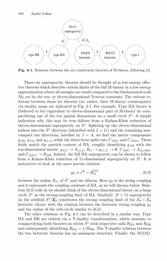
184 Andre Lukas
1
supergravityD=11
type IIB type IIAheterotic
E8xE8heteroticSO(32) type I
S / Z
T T S
S12
Fig. 6.1. Relation between the six constituent theories of M-theory, following [5].
These six supergravity theories should be thought of as low-energy effec-tive theories which describe certain limits of the full M-theory in a low-energyapproximation where all energies are small compared to the fundamental scaleMF set by the ten- or eleven-dimensional Newton constants. The various re-lations between those six theories (or, rather, their M-theory counterparts)via duality maps are indicated in Fig. 6.1. For example, Type IIA theory is(believed to be) equivalent to eleven-dimensional part of M-theory by com-pactifying one of the ten spatial dimensions on a small circle S1. A simpleindication why this may be true follows from a Kaluza-Klein reduction ofeleven-dimensional supergravity on S1. Splitting up the eleven-dimensionalindices into the S1 direction (identified with I = 11) and the remaining non-compact ten directions, labelled by I = A, we find the metric componentsgAB , gA11 and g11,11 while the three-form splits into CABC and CAB11. Thesefields match the particle content of IIA, roughly identifying gAB with theten-dimensional metric, gA11 → A(1)A, R11 → g11,11 → Φ, CABC → A(3)ABC
and CAB11 → BAB . Indeed, the full IIA supergravity can be shown to followfrom a Kalaza-Klein reduction of 11-dimensional supergravity on S1. It isinstructive to look at the more precise relation
gS ≡ eΦ ∼ R3/211 (6.3)
between the radius R11 of S1 and the dilaton. Here gS is the string couplingand it represents the coupling constant of IIA, as we will discuss below. Rela-tion (6.3) tells us we should think of the eleven-dimensional theory on a largecircle S1 as the strong-coupling limit of IIA. Similarly, D = 11 supergravityon the orbifold S1/Z2 constitutes the strong coupling limit of the E8 × E8heterotic theory with the relation between the heterotic string coupling gSand the radius of the orbi-circle similar to (6.3).
The other relations in Fig. 6.1 can be described in a similar way. TypeIIA and IIB are related via a T-duality transformation, which amounts tocompactifying both theories on circles S1 with respective radii RIIA and RIIBand subsequently identifying RIIA = 1/RIIB. The T-duality relation betweenthe two heterotic theories has an analogous structure. Finally, the SO(32)-
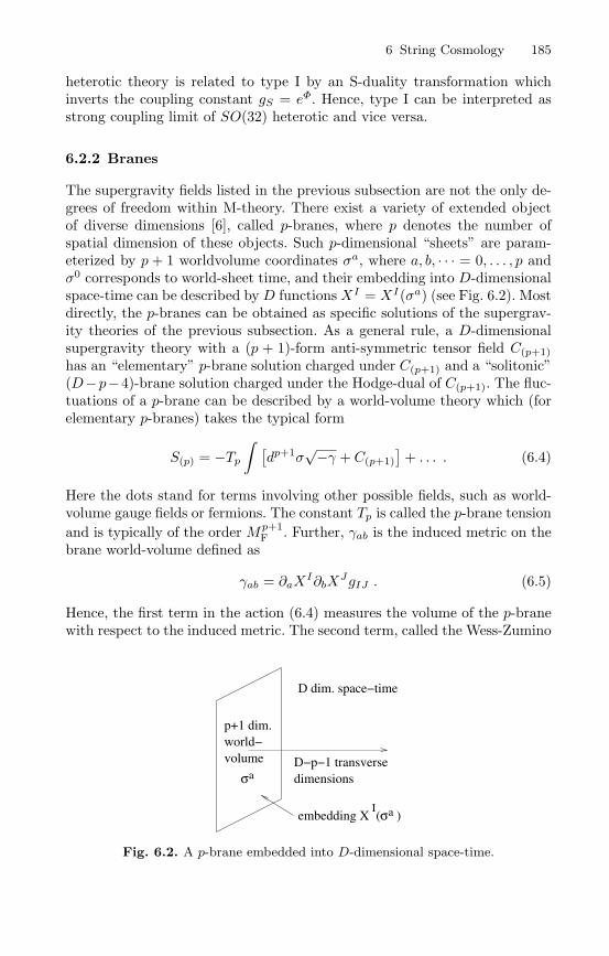
6 String Cosmology 185
heterotic theory is related to type I by an S-duality transformation whichinverts the coupling constant gS = eΦ. Hence, type I can be interpreted asstrong coupling limit of SO(32) heterotic and vice versa.
6.2.2 Branes
The supergravity fields listed in the previous subsection are not the only de-grees of freedom within M-theory. There exist a variety of extended objectof diverse dimensions [6], called p-branes, where p denotes the number ofspatial dimension of these objects. Such p-dimensional “sheets” are param-eterized by p + 1 worldvolume coordinates σa, where a, b, · · · = 0, . . . , p andσ0 corresponds to world-sheet time, and their embedding into D-dimensionalspace-time can be described byD functionsXI = XI(σa) (see Fig. 6.2). Mostdirectly, the p-branes can be obtained as specific solutions of the supergrav-ity theories of the previous subsection. As a general rule, a D-dimensionalsupergravity theory with a (p + 1)-form anti-symmetric tensor field C(p+1)has an “elementary” p-brane solution charged under C(p+1) and a “solitonic”(D−p−4)-brane solution charged under the Hodge-dual of C(p+1). The fluc-tuations of a p-brane can be described by a world-volume theory which (forelementary p-branes) takes the typical form
S(p) = −Tp
∫ [dp+1σ
√−γ + C(p+1)]+ . . . . (6.4)
Here the dots stand for terms involving other possible fields, such as world-volume gauge fields or fermions. The constant Tp is called the p-brane tensionand is typically of the order Mp+1
F . Further, γab is the induced metric on thebrane world-volume defined as
γab = ∂aXI∂bX
JgIJ . (6.5)
Hence, the first term in the action (6.4) measures the volume of the p-branewith respect to the induced metric. The second term, called the Wess-Zumino
D dim. space−time
D−p−1 transverse
p+1 dim.world−volume
aσ dimensions
Iembedding X (σa )
Fig. 6.2. A p-brane embedded into D-dimensional space-time.
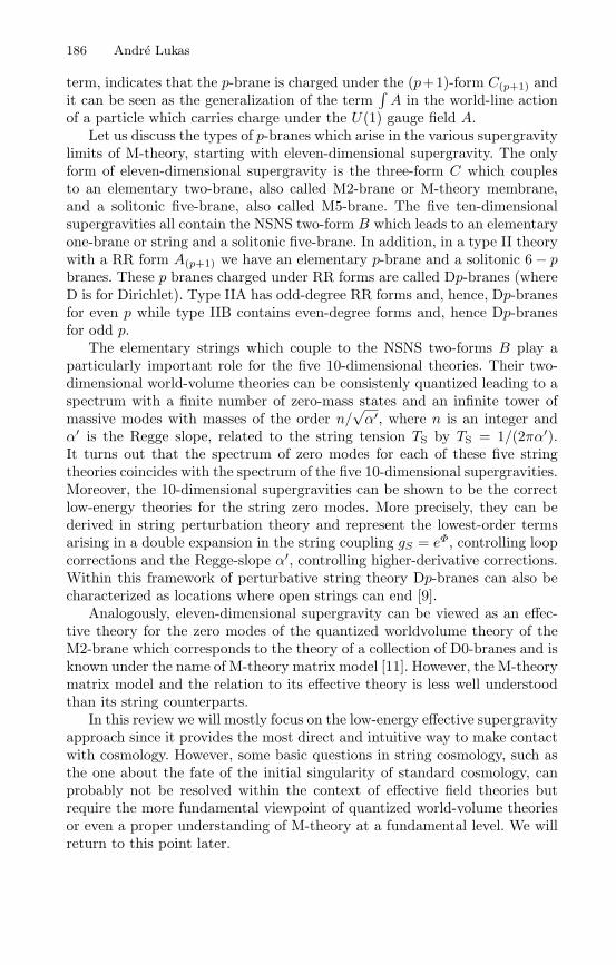
186 Andre Lukas
term, indicates that the p-brane is charged under the (p+1)-form C(p+1) andit can be seen as the generalization of the term
∫A in the world-line action
of a particle which carries charge under the U(1) gauge field A.Let us discuss the types of p-branes which arise in the various supergravity
limits of M-theory, starting with eleven-dimensional supergravity. The onlyform of eleven-dimensional supergravity is the three-form C which couplesto an elementary two-brane, also called M2-brane or M-theory membrane,and a solitonic five-brane, also called M5-brane. The five ten-dimensionalsupergravities all contain the NSNS two-form B which leads to an elementaryone-brane or string and a solitonic five-brane. In addition, in a type II theorywith a RR form A(p+1) we have an elementary p-brane and a solitonic 6 − pbranes. These p branes charged under RR forms are called Dp-branes (whereD is for Dirichlet). Type IIA has odd-degree RR forms and, hence, Dp-branesfor even p while type IIB contains even-degree forms and, hence Dp-branesfor odd p.
The elementary strings which couple to the NSNS two-forms B play aparticularly important role for the five 10-dimensional theories. Their two-dimensional world-volume theories can be consistenly quantized leading to aspectrum with a finite number of zero-mass states and an infinite tower ofmassive modes with masses of the order n/
√α′, where n is an integer and
α′ is the Regge slope, related to the string tension TS by TS = 1/(2πα′).It turns out that the spectrum of zero modes for each of these five stringtheories coincides with the spectrum of the five 10-dimensional supergravities.Moreover, the 10-dimensional supergravities can be shown to be the correctlow-energy theories for the string zero modes. More precisely, they can bederived in string perturbation theory and represent the lowest-order termsarising in a double expansion in the string coupling gS = eΦ, controlling loopcorrections and the Regge-slope α′, controlling higher-derivative corrections.Within this framework of perturbative string theory Dp-branes can also becharacterized as locations where open strings can end [9].
Analogously, eleven-dimensional supergravity can be viewed as an effec-tive theory for the zero modes of the quantized worldvolume theory of theM2-brane which corresponds to the theory of a collection of D0-branes and isknown under the name of M-theory matrix model [11]. However, the M-theorymatrix model and the relation to its effective theory is less well understoodthan its string counterparts.
In this review we will mostly focus on the low-energy effective supergravityapproach since it provides the most direct and intuitive way to make contactwith cosmology. However, some basic questions in string cosmology, such asthe one about the fate of the initial singularity of standard cosmology, canprobably not be resolved within the context of effective field theories butrequire the more fundamental viewpoint of quantized world-volume theoriesor even a proper understanding of M-theory at a fundamental level. We willreturn to this point later.

6 String Cosmology 187
6.2.3 Compactification
While there may be a number of cosmological problems which can be studiedin the context of a ten- or eleven-dimensional toy model it is quite clear thata successful model of string cosmology must evolve towards an effectivelyfour-dimensional state at late time. Moreover, this effective four-dimensionaltheory should reproduce the known features of particle physics, that is, theparticle physics standard model or some suitable (perhaps supersymmetric)extension thereof. In this review, I will discuss string cosmology in this spirit,aiming at combing the desired properties both from cosmology and particlephysics.
Let us begin by introducing some of the basic concepts of compactifi-cation. For more detailed accounts see, for example, [7]. Starting point isa particular class of solutions of one of the six supergravity theories whichmust respect four-dimensional Poincare invariance. Accordingly, the metricfor such solutions has the general structure
ds2 = e2A(y)dxµdxνηµν + gmn(y)dymdyn , (6.6)
where µ, ν, · · · = 0, 1, 2, 3 are four-dimensional indices and y = (ym) are thecoordinates of a six- or seven-dimensional internal compact spaceX with met-ric gmn. Note that four-dimensional Poincare invariance is compatible withthe so called warp factor exp(2A(y)) which multiplies the four-dimensionalpart of the metric, as long as this factor only depends on the internal coor-dinates y.
If all other background fields vanish the above metric must, to lowest or-der, be a solution of the free Einstein equations, that is, it must be Ricci-flat.This implies that the warp factor must be trivial, A = 0, and that the in-ternal metric gmn must be Ricci-flat. The simplest example for an internalspace is then a torus T 6 or T 7 with a flat metric. While such torus compact-ifications are interesting to study on theoretical grounds they do not breakany of the supersymmetries of the higher-dimensional theory and, therefore,lead to unrealistic four-dimensional models with sixteen or thirty two su-percharges, corresponding to N = 4 or N = 8, respectively. However, thereexist more complicated Ricci-flat spaces, namely Calabi-Yau three-folds [12](six-dimensional manifolds with holonomy SU(3)) or G2 spaces [13] (seven-dimensional spaces with holonomy G2) which reduce the amount of super-symmetry to 1/4 or 1/8, respectively. Hence, such manifolds or suitable sin-gular (orbifold) limits thereof, reduce the four-dimensional supersymmetryto a more suitable N = 1 or N = 2.
In more complicated cases, when fields other than the metric are non-trivial in the background, the warp-factor A can be non-vanishing and theinternal metric will be no longer Ricci-flat. Particularly interesting examplesare provided by flux compactifications [14, 16, 17, 18, 19, 20], where the fieldstrengths G(p) = dC(p) of anti-symmetric tensor fields are non-trivial on theinternal space.
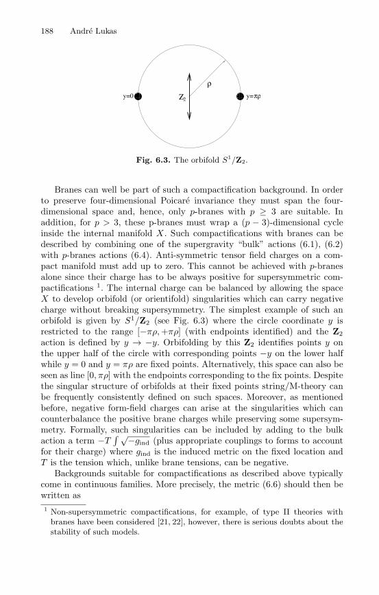
188 Andre Lukas
πρ
ρ
Ζ2y=0 y=
Fig. 6.3. The orbifold S1/Z2.
Branes can well be part of such a compactification background. In orderto preserve four-dimensional Poicare invariance they must span the four-dimensional space and, hence, only p-branes with p ≥ 3 are suitable. Inaddition, for p > 3, these p-branes must wrap a (p − 3)-dimensional cycleinside the internal manifold X. Such compactifications with branes can bedescribed by combining one of the supergravity “bulk” actions (6.1), (6.2)with p-branes actions (6.4). Anti-symmetric tensor field charges on a com-pact manifold must add up to zero. This cannot be achieved with p-branesalone since their charge has to be always positive for supersymmetric com-pactifications 1. The internal charge can be balanced by allowing the spaceX to develop orbifold (or orientifold) singularities which can carry negativecharge without breaking supersymmetry. The simplest example of such anorbifold is given by S1/Z2 (see Fig. 6.3) where the circle coordinate y isrestricted to the range [−πρ,+πρ] (with endpoints identified) and the Z2action is defined by y → −y. Orbifolding by this Z2 identifies points y onthe upper half of the circle with corresponding points −y on the lower halfwhile y = 0 and y = πρ are fixed points. Alternatively, this space can also beseen as line [0, πρ] with the endpoints corresponding to the fix points. Despitethe singular structure of orbifolds at their fixed points string/M-theory canbe frequently consistently defined on such spaces. Moreover, as mentionedbefore, negative form-field charges can arise at the singularities which cancounterbalance the positive brane charges while preserving some supersym-metry. Formally, such singularities can be included by adding to the bulkaction a term −T ∫ √−gind (plus appropriate couplings to forms to accountfor their charge) where gind is the induced metric on the fixed location andT is the tension which, unlike brane tensions, can be negative.
Backgrounds suitable for compactifications as described above typicallycome in continuous families. More precisely, the metric (6.6) should then bewritten as1 Non-supersymmetric compactifications, for example, of type II theories with
branes have been considered [21, 22], however, there is serious doubts about thestability of such models.

6 String Cosmology 189
ds2 = e2A(y,bi)dxµdxνgµν + gmn(y, bi)dymdyn , (6.7)
where gµν is the four-dimensional metric and bi are a number of continuousparameters or moduli. Geometrically, the moduli bi can usually be interpretedas the radii or cycle volumes of the internal manifold X. Further such modulican arise from zero modes of the form-fields and we will generically denotethese by νi. Zero modes can also arise from branes which are part of thebackground. They can be, for example, brane positions in the internal space orzero modes of other brane-world volume fields. All these zero modes becomefields in the four-dimensional effective theory and we now turn to discuss itsgeneric structure.
6.2.4 The Four-Dimensional Effective Theory
The four-dimensional effective theory can be viewed as a theory for the zeromodes (or collective modes) of a class of background geometries, In this re-view, I will focus on backgrounds which preserve four-dimensional N = 1supersymmetry which is the right amount to guarantee some degree of sta-bility of the backgrounds and allow for contact with particle physics. Hence,the effective theory must be a four-dimensional N = 1 supergravity theory.In the following I will assume familiarity with such supergravity theories. Fora pedagogical introduction see, for example, [23, 15].
The four-dimensional fields can be split into two groups according to theirhigher-dimensional origin. First, there are field which originate from the bulkand they account for gravity and all gravity-like fields, such as the bulkmoduli bi and νi. Secondly, there are four-dimensional fields which descendfrom branes and they should account for all the gauge and gauge matterfields. Accordingly, we split the chiral multiplets into two types 2, the modulimultiplets T i, typically containing a geometrical “radius” modulus bi and anaxion νi
T i = bi + iνi , (6.8)
and the brane gauge matter fields Ca. For a successful particle physics model,those latter fields should contain the spectrum of the (supersymmetric) stan-dard model. At the perturbative level and without flux, the Kahler potentialK, the superpotential W and the gauge-kinetic function f take the genericform
K = Kmod(T i, T i) + Zab(T i, T i)CaCb (6.9)W = dabc(T i)CaCbCc (6.10)f = f(T i) , (6.11)
2 However, not quite respecting our previous distinction we will also denote branemoduli, such as internal brane positions, as T i.
190 Andre Lukas
where Kmod is the moduli Kahler potential, Zab is the (moduli-dependent)matter field Kahler metric and dabc are (moduli-dependent) Yukawa cou-plings. Higher order terms in C from both K and W have been dropped.When flux or non-perturbative effects are included the most important ad-dition to the above structure is the introduction of an additional modulisuperpotential Wmod(T i). The validity of the effective theory is restricted bywhatever restricted the validity of the original higher-dimensional theory itdescended from, by possible constraints from the validity of the backgroundsolutions plus the requirement that all energies be smaller than 1/Rc, whereRc is the typical compactification radius.
Before going into more detail, it is worth noting that the above theoriesprovide plenty of scope for time-varying coupling constants, a topic of someinterest in cosmology. In this review, we will not discuss this subject in anydetail.
A central issue for cosmology as well as particle physics is the dynamicsof the moduli fields T i. Let us, therefore, consider some typical expressionsfor the moduli Kahler potential and superpotential. For a generic modulusT = b+ iν the Kahler potential frequently takes the form
Kmod = −k ln(T + T ) , (6.12)
where k is a constant. The associated kinetic terms for b and ν are then
k
b2(∂µb∂
µb+ ∂µν∂µν) . (6.13)
This implies the canonically normalized field is β defined by
b = exp(β√k
). (6.14)
Typical moduli superpotentials contain terms
Wmod ∼e−cT
T, (6.15)
where the upper contribution originates from non-perturbative sources suchas gaugino-condensation [14, 15] or brane instantons [24, 25] and the lowercontribution originates from flux3. Note that in terms of the canonicallynormalized field β non-perturbative terms are double-exponential while fluxterms are single-exponential.
Recall that the scalar potential in four-dimensional N = 1 supergravityfor a collection φI of chiral multiplets is given by
V = eK[KIJFI FJ − 3|W |2] , (6.16)
3 Flux superpotentials can be more complicated functions of the moduli but, unlikenon-perturbative contributions, they are not exponential in T .

6 String Cosmology 191
b0
V(b)
Fig. 6.4. Typical shape of the potential in the direction of a radius modulus b.
whereFI =
∂W
∂φI+∂K
∂φIW , (6.17)
and KIJ is the inverse of the Kahler metric
KIJ =∂2K
∂φI∂φJ. (6.18)
This can be used to calculate the potential for moduli Kahler potentials of thetype (6.12) and moduli superpotentials which are a sum of the possible con-tributions in (6.15). In the axion direction ν, such potentials usually have anumber of substantial minima (in the absence of flux the potential is, in fact,periodic in ν). A typical shape in the b direction has been sketched in Fig. 6.4.Such a runaway shape without a minimum arises for a single non-perturbativeterm [14] a sum of such terms unless carefully tuned [26] or simple flux-onlysuperpotentials (the tail falling off double-exponential or exponential in β de-pending on the case). A more interesting situation with a minimum at finiteb and a negative cosmological constant can be achieved for a carefully tunedsuperposition of non-perturbative contributions [26] or, much more generi-cally, by the superposition of a non-perturbative and a flux term entering Wwith different signs [14, 27]. Such a shape has been sketched in Fig. 6.5. Notethat the value of b at the minimum normally corresponds to compactificationradii not too far away from the fundamental length scale 1/MF of the theory.From our current understanding it seems unlikely, therefore, that scenarioswith very large additional dimensions [1, 2] can be embedded into M-theory.There are indications [27] that the minimum in Fig. 6.5 can be lifted to a pos-itive cosmological constant by inclusion of certain supersymmetry breakingeffects, such as anti-branes and that all moduli can be stabilized for certainconstructions. This would result in a shape as shown in Fig. 6.6. A majorproblem in extracting concrete predictions from string theory is its large vac-uum degeneracy. One manifestation of this degeneracy is the presence of themoduli which, we recall, parameterize classes of background solutions. Aswe have seen above, through the inclusion of moduli potentials one can at

192 Andre Lukas
b0
V(b)
Fig. 6.5. Potential with negative cosmological constant minimum in the directionof a radius modulus b.
b0
V(b)
Fig. 6.6. Potential with positive cosmological constant minimum in the directionof a radius modulus b.
least begin to address the dynamics of these fields and, perhaps, single outa background geometry by fixing the moduli. We will return to this point inSect. 6.4 when we discuss inflation. However, a different type of degeneracyarises from the existence of a large number of topologically different classesof backgrounds (see Fig. 6.7). They arise, for example, from topogically dif-ferent internal manifold X or topologically different brane configurations.Low-energy theories associated to different topologies can be vastly different,such as in their particle spectrum or gauge group. The problem how to singleout a specific topology is largely unsolved even in principle. We will returnto this issue in Sect. 6.5 when we discuss topology change.
6.2.5 A Specific Example: Heterotic M-Theory
Let us now illustrate the previous general discussion with a concrete classof examples within heterotic M-theory [28]. The construction starts witheleven-dimensional supergravity (6.1) on the orbifold S1/Z2 which has beendescribed in Sect. 6.2.3. In addition to the fields of eleven-dimensional super-gravity, this introduces two ten-dimensional E8 super-Yang-Mills multiplets,one an each of the ten-dimensional orbifold fixed planes (boundaries). This

6 String Cosmology 193
2
D=11 SUGRA
D=5, N=1 SUGRA
D=4, N=1
D=10E 8
SYM
D=10E 8
SYM
5brane
on CY
N=1D=4
brane3
N=1D=4
on S / Z1
Fig. 6.7. Reduction of heterotic M-theory to five and four dimensions.
theory constitutes the strong coupling limit of the E8 × E8 heterotic string(see Fig. 6.1) in much the same way eleven-dimensional supergravity is thestrong coupling limit of IIA.
Upon reduction of this theory on Calabi-Yau three-folds [29, 30] one ob-tains a class of five-dimensional brane-world theories with a bulk describedby five-dimensional N = 1 supergravity and coupled to two four-dimensionalN = 1 theories localized on the two, now four-dimensional boundaries M1and M2. There exist examples where the theory on one of the boundaries isvery close to the (supersymmetric) standard model of particle physics [31, 32]and one expects a large number of such examples to exist. Further, one canintroduce M5-branes wrapping two-cycles within the Calabi-Yau three-foldinto the compactification. In the five-dimensional brane-world theory, theybecome 3-branes which also carry a four-dimensional N = 1 theory. Forsimplicity, we consider a single such 3-brane which (together with its Z2 mir-ror) we denote by M3. Taking the radius of the orbifold sufficiently smallone can further derive an effective four-dimensional N = 1 theory. The twosteps of this reduction are summarized in Fig. 6.7. A minimal version offive-dimensional heterotic M-theory is given by [30, 33]
S = Sbulk +3∑
n=1
Sn , (6.19)
194 Andre Lukas
where
Sbulk = − 12κ2
5
∫d5x
√−g[12R+
14∂ϕ2 +
13α2e−2ϕ
](6.20)
Sn = − 1κ2
5
∫
Mn
d4x√−g4αne
−ϕ for n = 1, 2 (6.21)
S3 = − 12κ2
5
∫
M3
√−γ|α3|e−ϕ . (6.22)
Here, we have only kept the minimal field content and have, in particular,omitted gauge and matter fields from the boundary actions S1 and S2. Morecomplete actions can be found in [29, 34]. The parameter α which appears inthe bulk potential is defined by
α =3∑
n=1
αnθ(Mn) , (6.23)
where θ is the theta function. The boundary charges α1, α2 and the 3-branecharge α3 have to satisfy
3∑
n=1
αn = 0 , (6.24)
so that the total charge is zero. We note that the boundary tensions can benegative (since α1 and α2 can be) while the three-brane tension is alwayspositive, as it should. For α3 > 0 we have a three-brane and the theory issupersymmetric as described above. We can also consider the case of an antithree-brane, taking α3 < 0. In this case supersymmetry is completely broken.The scalar field ϕ is the five-dimensional dilaton and eϕ is proportional tothe volume of the internal Calabi-Yau three-fold.
The associated four-dimensional effective N = 1 theory (for α3 > 0)can be obtained as the theory for the collective modes of a class of domainwall solutions of the above five-dimensional action [30]. It contains threegeometrical moduli, namely β ∼ ln < g55 > measuring the radius of theorbifold, φ ∼< ϕ > which measures the volume of the Calabi-Yau space andz ∈ [0, 1] which specifies the position of the 3-brane (where z = 0 and z = 1correspond to the boundaries M1 and M2, respectively). Along with thesefields go three chiral superfields
S = eφ + . . .T = eβ + . . . (6.25)Z = eβz + . . .
where the dots indicate axion and higher-order terms. The Kahler potentialfor these moduli is given by [35, 34]
6 String Cosmology 195
Kmod = − ln[S + S − q3 (Z + Z)2
T + T
]− 3 ln(T + T ) , (6.26)
where q3 is a constant proportional to α3. Non-perturbative potentials takethe general form
Wmod ∼ exp(−c1S + c2T + c3Z) , (6.27)
with positive constants cn while a flux superpotential is a constant 4 in S, Tand Z.
We stress that the above four-dimensional effective theory is in gen-eral different from the four-dimensional “on-the-brane” theory obtained byprojecting the five-dimensional brane-world theory onto one of the bound-aries. The four-dimensional effective theory provides a valid description of allfive-dimensional dynamics sufficiently close to the domain wall vacua of thefive-dimensional theory. The “on-the-brane” theory, on the other hand, pro-vides an incomplete description of all solutions of the five-dimensional theory.Therefore, working with the “on-the-brane” theory can be misleading in thatit suggests four-dimensional physics while, in fact, it may describe situationsfor away from the effective four-dimensional limit required at late time.
We have argued above, that compact dimensions in M-theory are un-likely to be much larger than the fundamental length scale of the theory.Accordingly, most of the evolution can be safely described in terms of theeffective four-dimensional theory. Only in the very early universe, possiblyduring inflation, and if the orbifold size is relatively large may working withthe five-dimensional theory be required.
6.3 Classes of Simple Time-Dependent Solutions
At the heart of cosmological models is a background solution with a four-dimensional space-time metric of Friedmann-Robertson-Walker (FRW) type.Finding FRW solutions in the context of M-theory, therefore, seems to bea natural starting point for M-theory cosmology. In this section, we presentsimple classes of such solutions and discuss their properties. For an extensivelist of references to the vast literature on the subject see, for example, [37].
6.3.1 Rolling Radii Solutions
We would now like to consider the free evolution (that is, the potential is setto zero) of a number of four-dimensional moduli fields bi = exp(βi) whichmeasure radii of the internal manifold X. Such solutions are also referredto as rolling radii solutions [38] and are the analogue of Kasner solutions in4 However, it depends on another class of moduli, the complex structure moduli
which we have not discussed explicitly. Their values are usually fixed by the fluxpotential [36].
196 Andre Lukas
M-theory. As we have explained in Sect. 6.2.4, moduli potentials in M-theoryrapidly decrease for large values of the radius moduli. Hence, rolling radiisolutions should provide a good approximation to the dynamics at sufficientlylarge values of the radii.
Let us start with a class of examples [39] which arises in the contextof compactifying eleven-dimensional supergravity on a manifold of G2 holon-omy. The G2 manifolds under consideration have seven radius moduli βi withassociated chiral multiplet T i = exp(βi) + axion plus a number of additionalmoduli which we suppress. The full model has been analyzed in [40]. The T i
part of the Kahler potential is simply
Kmod = −7∑
i=1
ln(T i + T i) , (6.28)
One can consistently set the axions in T i to constants which results in thesimple Lagrangian
L = −√−g[
R+7∑
i=1
∂βi∂βi
]
. (6.29)
Consider an Ansatz with time-dependent moduli βi = βi(t) and a FRWmetric
ds2 = −dt2 + e2α(t)dx2 (6.30)
with scale factor α and, for simplicity, flat spatial sections. The solutions arethen given by
a ≡ eα ∼ |t| 13 (6.31)
βi = pi ln |t| + ci . (6.32)
The expansion powers p = (pi) are constrained by
p2 =43, (6.33)
while ci are arbitrary constants. Note that the expansion power of the scalefactor a is 1/3, as expected for a kinetic energy driven expansion. Everyone of the above solutions exists on two branches, the positive-time branch,t > 0, which begins in a curvature singularity and corresponds to sub-luminal expansion of the universe and the negative-time branch, t < 0, whichends in a curvature singularity and describes super-luminal contraction. Ofcourse, close to the singularity in either branch the four-dimensional effectivefield theory breaks down as higher-derivative corrections become important.Whether and how this singularity is regulated in the full M-theory must stillbe viewed as an open question to which we return in Sect. 6.4.3. We also notethat the power-law evolution of the scalar fields βi describes the expansionor contraction of the internal G2 space X.
6 String Cosmology 197
Another, similar class of rolling radii solutions can be obtained in thecontext of four-dimensional heterotic M-theory without five-branes. We startwith the Kahler potential (6.26), drop the five-brane modulus Z and writeS = eφ + axion, T = eβ + axion. This leads to the Lagrangian
L = −√−g[R+
12(∂φ)2 +
32(∂β)2
]. (6.34)
For a FRW metric (6.30) and time-dependent fields φ = φ(t), β = β(t) onefinds the solutions
a ∼ |t| 13
φ = pφ ln |t| + cφ (6.35)β = pβ ln |t| + cβ .
The expansion powers cφ and cβ satisfy
3p2β + p2φ =43, (6.36)
while cφ and cβ are arbitrary constants. Recall that φ and β describe theevolution of the Calabi-Yau volume and the radius of the orbifold S1/Z2,respectively.
6.3.2 Including Axions
Recall that axions νi usually arise as zero modes of the anti-symmetric tensorfields of M-theory and, at low energy, become the imaginary parts of themoduli multiplets T i = exp(βi)+ iνi. Consider a single such axion ν coupledto a number of radius moduli βi. The Lagrangian (6.29) is then modified to
L = −√−g[
R+∑
i
∂βi∂βi + exp
(∑
i
qiβi
)
∂ν∂ν
]
. (6.37)
Here q = (qi) is a constant vector which depends on the specific case underconsideration. The general solution for this Lagrangian with time-dependentscalar fields and a FRW metric (6.30) can be found [41, 42] analytically. Hereit will be sufficient to describe the qualitative behaviour of this solution.In each branch a solution to (6.37) has an early and a late asymptotic re-gion where ν is approximately constant and the evolution of βi is describedby a rolling radii solution (6.32) with expansion power p(i) for the initialasymptotic state and a generally different expansion power p(f) for the finalasymptotic state. The two asymptotic regions are connected by an interme-diate phase where the axion ν moves by a finite distance in field space. It canbe shown that the initial and final expansion powers are related by
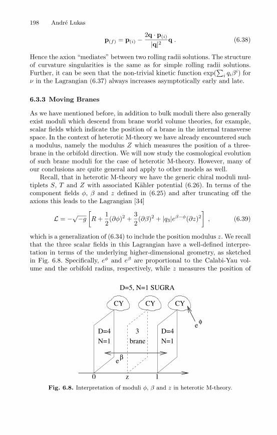
198 Andre Lukas
p(f) = p(i) − 2q · p(i)
|q|2 q . (6.38)
Hence the axion “mediates” between two rolling radii solutions. The structureof curvature singularities is the same as for simple rolling radii solutions.Further, it can be seen that the non-trivial kinetic function exp(
∑i qiβ
i) forν in the Lagrangian (6.37) always increases asymptotically early and late.
6.3.3 Moving Branes
As we have mentioned before, in addition to bulk moduli there also generallyexist moduli which descend from brane world volume theories, for example,scalar fields which indicate the position of a brane in the internal transversespace. In the context of heterotic M-theory we have already encountered sucha modulus, namely the modulus Z which measures the position of a three-brane in the orbifold direction. We will now study the cosmological evolutionof such brane moduli for the case of heterotic M-theory. However, many ofour conclusions are quite general and apply to other models as well.
Recall, that in heterotic M-theory we have the generic chiral moduli mul-tiplets S, T and Z with associated Kahler potential (6.26). In terms of thecomponent fields φ, β and z defined in (6.25) and after truncating off theaxions this leads to the Lagrangian [34]
L = −√−g[R+
12(∂φ)2 +
32(∂β)2 + |q3|eβ−φ(∂z)2
], (6.39)
which is a generalization of (6.34) to include the position modulus z. We recallthat the three scalar fields in this Lagrangian have a well-defined interpre-tation in terms of the underlying higher-dimensional geometry, as sketchedin Fig. 6.8. Specifically, eφ and eβ are proportional to the Calabi-Yau vol-ume and the orbifold radius, respectively, while z measures the position of
1
CY CY CY
D=4N=1
3brane
D=4N=1
e
z
φ
βe
D=5, N=1 SUGRA
0
Fig. 6.8. Interpretation of moduli φ, β and z in heterotic M-theory.
6 String Cosmology 199
the three-brane with z = 0 and z = 1 corresponding to the locations of theboundaries.
An elementary observation about the Lagrangian (6.39) is the existenceof the non-trivial kinetic term for the brane position modulus z. This termimplies that the bulk moduli φ and β necessarily vary in time whenever zdoes. As we will see this variation of the bulk moduli is actually importantand has important implications for the qualitative features of the solutions.It would, therefore, be quite inappropriate, in this model as well as in otherbrane models, to study the evolution of the brane in a static background.
We note that the Lagrangian (6.39) is a special case of the Lagrangian(6.37) which couples radius moduli to an axion, with the position modulusz formally playing the role of the axion. Hence, we conclude that the cosmo-logical solutions [43] to (6.39) have two asymptotic regions where the braneis approximately in rest and φ and β evolve as rolling radii with expansioncoefficients satisfying (6.36). These two asymptotic early and late regions areconnected by a period where the brane moves by a finite coordinate dis-tance. In short, the brane evolution interpolates between two rolling radiisolutions. Since the brane moves by a finite distance it may or may not col-lide with one of the boundaries depending on initial conditions. In the caseof collision, the system may undergo a topology-changing small instantontransition [44, 45, 46] where the three-brane is “absorbed”. Some dynamicalaspects related to this transition have been studied in [47]. We also note thatthe heterotic strong coupling expansion parameter defined by εS ∼ exp(β−φ)always increases asymptotically for those solutions. Hence the effective the-ory is always invalidated asymptotically, a fact one would have missed hadone set the bulk moduli to constants.
6.3.4 Duality Symmetries and Cosmological Solutions
Dualities are global, discrete transformations on the M-theory moduli spacewhich are thought to be exact symmetries of the theory. They can usuallybe found as symmetries of low-energy effective theories and, at perturbativelevel, they enlarge to continuous version of the symmetry. A typical examplefor a Kahler simple potential
Kmod = −k ln(T + T ) (6.40)
with a constant k would be given by the transformations
T → aT + ibcT + id
, (6.41)
where ad − bc = 1 which form the group SL(2, R). The invariance of theaction can be seen by noting that these transformation can be generated byT → aT+ib and T → 1/T where the former obviously leaves the above Kahlerpotential invariant (up to an irrelevant constant) and the latter correspondsto a Kahler transformation of Kmod which leaves the action unchanged.
200 Andre Lukas
Such continuous versions of duality symmetries can be quite useful togenerate new cosmological solutions from old ones [37]. For example, theabove transformations mix the real and imaginary part of T and can, hence,be used to generate solutions with a non-trivial axion (the imaginary part ofT ) from pure rolling radii solutions.
6.4 M-Theory and Inflation
The dynamics of scalar fields and inflation in particular constitutes proba-bly the most important area in which one expects a close relation betweencosmology and particle physics (or fundamental theories in general). Let us,therefore, discuss inflation in the context of M-theory in some detail.
6.4.1 Reminder Inflation
In this review, I will understand “inflation” as an era in the history of theuniverse where modes leave the Hubble horizon. The ratio of the size of aparticular mode and the horizon size is proportional to |H|a where a = expαis the scale factor in (6.30) and H = a/a. Modes leave the Hubble horizon ifthe time-derivative of |H|a is positive. For a power-law evolution with
a ∼ |t|p (6.42)
and some constant power p this implies that
d
dt(|H|a) = sgn(t)a ∼ sgn(t)p(p− 1)|t|p−2 (6.43)
must be positive for inflation. This leads to two different possibilities. First,in the positive-time branch, t > 0, we should have p > 1. This case is realizedby potential-driven inflation [48] which can arise if the potential5 V = V (φ)satisfies the slow-roll conditions
ε ∼(V ′
V
)2
1 , η ∼ V ′′
V 1 , (6.44)
in any part of fields space. Here the prime denotes the derivative with respectto the (canonically normalized) field φ.
The second case, for which (6.43) is positive arises in the negative-timebranch, t < 0, if p ∈ [0, 1]. This possibility is realized by many solutions inthe negative-time branch and is also referred to as pre-big-bang inflation [49,50]. Note, that in this case inflation evolves towards an apparent curvaturesingularity which arises within the low-energy effective theory.5 Here, φ is a generic scalar field.

6 String Cosmology 201
All proposed mechanisms (known to me) to solve the problems of standardcosmology fall into one of these two categories. This includes more recentproposals which involve moving branes such as the one in [51].
We will now discuss these two different types of inflation separately in thecontext of M-theory.
6.4.2 Potential-Driven Inflation
M-theory low-energy effective theories typically contain a large number ofscalar fields and inflation, if realized at all, is unlikely to arise in the formof one of the simple single-scalar field models which is commonly studied ininflationary model-building. The possibilities can be broadly classified into“bulk field inflation” where the inflaton is a combination of bulk scalar fieldsand “brane field inflation” where inflation arises from the evolution of scalarfields which originate from brane world-volume theories.
We start discussing bulk field inflation. The obvious problem in this caseis to find a suitable M-theory potential for bulk moduli which satisfies theslow-roll conditions (6.44) at least in some part of moduli space. For multi-field potentials these conditions have to be imposed on all directions in fieldspace which are not stabilized. In Sect. 6.2.4 we have discussed typical shapesfor such potentials in the direction of radius moduli. The generic problem isthat the potentials originating from superpotentials (6.15) are normally tosteep to be compatible with slow-roll. Hence, for potentials with a shape asin Fig. 6.4 there is little hope for any relevant amount of inflationary ex-pansion [52, 53], even though other directions in field space, such as someof the axion directions, may well be compatible with slow-roll. The situa-tion is somewhat more promising with potentials such as in Fig. 6.5 whichhave a minimum with negative cosmological constant in the direction of theradius moduli. Some inflation will be possible starting from the maximum(although a sufficient amount is likely to require initial conditions fine-tunedto the maximum) but the final state with negative cosmological constant isunattractive given the observational evidence for a positive cosmological con-stant in the late universe. There are indications for the existence of minimawith positive cosmological constant [27] such as in Fig. 6.6. In this case, themost promising scenario may be to interpret the minimum as the true late-time vacuum. Inflation may then be generated by fixing the radius moduli atthe minimum and use an axion direction or a brane field [54] as the inflaton.
With these remarks on bulk field inflation in mind we now turn to branefield inflation. A recently much discussed example of this type is anti-braneinflation [55], where the inflaton is the position modulus of an anti-brane. Letus discuss this mechanism in the context of heterotic M-theory with an anti5-brane. The effective four-dimensional theory for this situation is given by(6.39) with an additional potential
V ∼ (|q3| − q3)e−φ−2β
[1 − 2
3q1e
β−φz
]−1
. (6.45)

202 Andre Lukas
Recall that the anti-brane case corresponds to q3 < 0 where this potentialis indeed non-vanishing. Here, q1 is proportional to the charge α1 on theboundary at y = 0. This potential satisfies the slow-roll conditions in thez-direction as long as the strong coupling expansion parameter εS ∼ eβ−φ ismuch smaller than one, a condition that is anyway required for the validityof the effective theory. On would, therefore, hope for an inflationary periodwhile the anti-brane slowly moves along the orbifold direction which endswhen it collides with one of the boundaries. An obvious problem (which isquite generic for such anti-brane models) is that the potential (6.45) is byno means slow-roll in the direction of the radius moduli φ and β. Withoutany additional mechanism to stabilize the radius moduli no inflation will begenerated, therefore. The obvious solution seems to be to combine a potentialas in Fig. 6.6 which stabilizes the radius moduli with (6.45). Unfortunately,it turns out, the amount of inflation generated before the brane collides withthe boundary is too small. Roughly, this happens because the kinetic functionfor z in (6.39) is identical to the parameter εS which controls the slow-rollproperties of the potential (6.45). Again this problem arises in many typesof anti-brane inflation models, although it can be avoided in some construc-tions [56].
There is no need to insist on the anti-brane position modulus as theinflaton. There will generically be many brane scalar fields, such as the scalarpartners of matter fields, with polynomial superpotentials as in (6.10), whichmay be well-suited. These possibilities will now have to be examined for stringvacua with moduli potentials as in Fig. 6.6 and all moduli fixed.
So far we have exclusively focused on inflation in the context of an effectivefour-dimensional theory. As mentioned before, the reason is that the existenceof very large additional dimensions seem unlikely given the known mechanismof stabilizing moduli in M-theory. However, the energy scale during inflationcan be quite large (up to ∼ 1016GeV) and, hence, inflation may be able toprobe dimensions one or two orders of magnitude larger than the fundamentallength scale 1/MF . Such a possiblity may exist within heterotic M-theory [33]where coupling unification suggest a “largish” orbfield size [57]. In this case,the analysis should be carried out in the context of five-dimensional heteroticM-theory reviewed in Sect. 6.2.5. For further discussions in this directionsee [58].
6.4.3 Pre-Big-Bang Inflation
The basic idea of pre-big-bang cosmology [49, 50, 37] is to use solutions inthe negative-time branch to generate inflation. We note that this mechanismby itself is not particularly “stringy”. It simply relies on the existence of atime-reflection symmetry of General Relativity and can, hence, be used inany type of gravitational theory.
However, implementing the idea in a string context is rather straightfor-ward. Consider the heterotic Lagrangian (6.34) for the moduli φ and β with
6 String Cosmology 203
its cosmological solutions (6.35). Since the expansion power of the scale fac-tor is always 1/3 (and, hence, in the range [0, 1]) any of these solutions inthe negative time branch can be used to generate pre-big-bang inflation. Theoriginal model [49] focused on the special case of constant β, that is, pβ = 0which, from (6.36) implies a dilaton expansion power
pφ = ± 2√3. (6.46)
Of course, more complicated versions of the model with evolving β or withan additional moduli potential added to (6.34) are possible.
The obvious problem of this proposal is the future curvature singularityof negative-time branch solutions together with the necessity to generate atransition from the negative-time branch with contracting universe to stan-dard cosmology in the positive-time branch. Clearly, positive- and negative-time branch solutions cannot be simply continuously matched together sincethey correspond to opposite signs of the Hubble parameter. Hence, additionalphysics not contained in simple effective Lagrangian such as (6.34) must beresponsible for this hypothetical transition which has also been called “grace-ful exit” [59]. Let us briefly discuss why it is not easy to find a mechanismfor a graceful exit. Consider, the second order equation for the scale factor
H = −(ρ+ p) , (6.47)
where ρ and p are the total energy density and pressure for the model in-cluding contributions from whatever is supposed to generate the exit. For therequired transition from a state with negative H to a state with positive Hone needs stress energy which satisfies ρ+ p < 0, at least for some period oftime around the transition. However, most “decent” sources of stress energysuch as scalar fields with potentials, gauge fields, forms etc. satisfy the nullenergy condition ρ + p ≥ 0, simply from the algebraic form of their stressenergy tensor.
A form of stress energy which potentially does violate the null energycondition are higher curvature terms, such as R2 terms. It is well-known thatsuch terms arise in string theory as higher-order α′ corrections. Clearly, suchterms will become important when the pre-big-bang phase approaches thecurvature singularity. The hope has, therefore, been that string theory willsomehow regulate the curvature singularity, thereby generating a gracefulexit.
The question whether and how string theory resolves cosmological singu-larities has been addressed in different frameworks. Effective actions includinghigher-order α′ corrections and loop corrections have been studied [60, 61].Although, there are some indications that an exit can be achieved within thisframework there is an obvious problem with keeping only the lowest ordercorrections of an infinite series when these lowest order corrections need to belarge to generate the exit. It is hard to see how this problem can be overcome

204 Andre Lukas
in the context of an effective field theory approach. On a more fundamentallevel, there have been studies of exact string backgrounds in the context ofWess-Zumino-Witten models [62] and, more recently, a perturbative stringanalysis of time-dependent orbifolds [63]. It is fair to say that none of theseapproaches has led, so far, to conclusive results about the fate of cosmologicalsingularities in M-theory.
There has been some renewed interest [51] in pre-big-bang cosmologyin the context of negative-time branch solutions with a moving three-branewithin heterotic M-theory, based on the Lagrangian (6.39) (possibly with anadditional moduli potential). For example, one could use the negative-timebranch of the solutions described in Sect. 6.3.3 as the basis for a moving-brane pre-big-bang cosmology. While this proposal is nothing new in termsof the mechanism for inflation it contains an interesting new aspect related tothe exit problem. In the pre-big-bang phase, the three-brane can be arrangedto collide with one of the boundaries well before the system runs into largecurvature. The hope is that the brane-collision and the possible associatedtopology change ends the pre-big-bang phase and generates a graceful exit.This idea seems quite appealing in that it avoids the difficult problem ofdealing with the large-curvature region. However, it is far from clear at presentthat such a brane-boundary collision can indeed lead to an exit from the pre-big-bang phase.
A final remark on the calculation of scalar density perturbations in pre-big-bang models is in order. As a general rule, while potential-driven inflationgenerically leads to a scale-invariant spectrum with spectral index n close toone, spectral indices in the context of pre-big-bang cosmology vary substan-tially and depend on the particular solution. For example, the spectral indexfor an axion field in a background of one of the solutions (6.35) depends on pφ
and pβ [37]. Frequently, n is substantially larger than one. Moreover, it is notcompletely clear how to match perturbations across the transition from pre-to post-big-bang cosmology, a fact which has been highlighted in the recentdebate [64]. Presumably, the question of how this should be done can onlybe conclusively answered once a physical exit mechanism has been found.
6.5 Topology Change in Cosmology
As we have mentioned before, M-theory has a large number of topologicallydifferent compactifications. At present, it is unclear what, if anything, willchoose one particular topology over the others. It may well be that the cos-mological evolution has some role to play in this context. Fortunately, withinM-theory the topology of a compactification can change in a number of well-defined processes. Hence, one can think of the M-theory moduli space as oneentity (or, at least few entities) which consists of a web of different topologiesconnected by topology-changing processes. Indeed, such a picture seems to bea pre-requisite for any mechanism which would single out a particular topol-
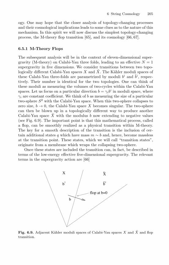
6 String Cosmology 205
ogy. One may hope that the closer analysis of topology-changing processesand their cosmological implications leads to some clues as to the nature of thismechanism. In this spirit we will now discuss the simplest topology-changingprocess, the M-theory flop transition [65], and its cosmology [66, 67].
6.5.1 M-Theory Flops
The subsequent analysis will be in the context of eleven-dimensional super-gravity (M-theory) on Calabi-Yau three folds, leading to an effective N = 1supergravity in five dimensions. We consider transitions between two topo-logically different Calabi-Yau spaces X and X. The Kahler moduli spaces ofthese Calabi-Yau three-folds are parametrized by moduli bi and bi, respec-tively. Their number is identical for the two topologies. One can think ofthese moduli as measuring the volumes of two-cycles within the Calabi-Yauspaces. Let us focus on a particular direction b = γib
i in moduli space, whereγi are constant coefficient. We think of b as measuring the size of a particulartwo-sphere S2 with the Calabi-Yau space. When this two-sphere collapses tozero size, b → 0, the Calabi-Yau space X becomes singular. The two-spherecan then be blown up in a topologically different way to produce anotherCalabi-Yau space X with the modulus b now extending to negative values(see Fig. 6.9). The important point is that this mathematical process, calleda flop, can be smoothly realized as a physical transition within M-theory.The key for a smooth description of the transition is the inclusion of cer-tain additional states q which have mass m ∼ b and, hence, become masslessat the transition point. These states, which we will call “transition states”,originate from a membrane which wraps the collapsing two-sphere.
Once these states are included the transition can, in fact, be described interms of the low-energy effective five-dimensional supergravity. The relevantterms in the supergravity action are [66]
flop at b=0
X X~
bi
b
bi~
Fig. 6.9. Adjacent Kahler moduli spaces of Calabi-Yau spaces X and X and floptransition.
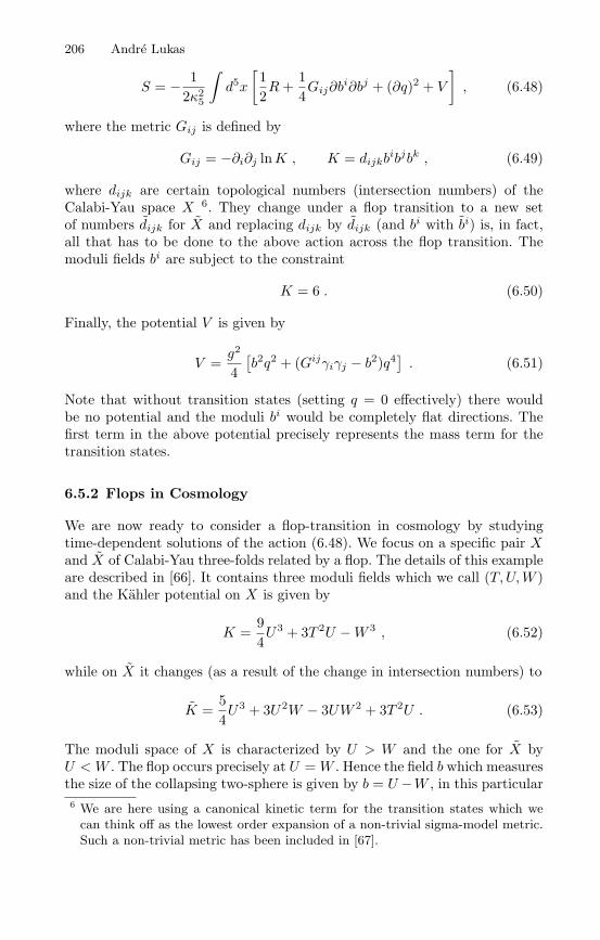
206 Andre Lukas
S = − 12κ2
5
∫d5x
[12R+
14Gij∂b
i∂bj + (∂q)2 + V], (6.48)
where the metric Gij is defined by
Gij = −∂i∂j lnK , K = dijkbibjbk , (6.49)
where dijk are certain topological numbers (intersection numbers) of theCalabi-Yau space X 6. They change under a flop transition to a new setof numbers dijk for X and replacing dijk by dijk (and bi with bi) is, in fact,all that has to be done to the above action across the flop transition. Themoduli fields bi are subject to the constraint
K = 6 . (6.50)
Finally, the potential V is given by
V =g2
4[b2q2 + (Gijγiγj − b2)q4] . (6.51)
Note that without transition states (setting q = 0 effectively) there wouldbe no potential and the moduli bi would be completely flat directions. Thefirst term in the above potential precisely represents the mass term for thetransition states.
6.5.2 Flops in Cosmology
We are now ready to consider a flop-transition in cosmology by studyingtime-dependent solutions of the action (6.48). We focus on a specific pair Xand X of Calabi-Yau three-folds related by a flop. The details of this exampleare described in [66]. It contains three moduli fields which we call (T,U,W )and the Kahler potential on X is given by
K =94U3 + 3T 2U −W 3 , (6.52)
while on X it changes (as a result of the change in intersection numbers) to
K =54U3 + 3U2W − 3UW 2 + 3T 2U . (6.53)
The moduli space of X is characterized by U > W and the one for X byU < W . The flop occurs precisely at U =W . Hence the field b which measuresthe size of the collapsing two-sphere is given by b = U −W , in this particular6 We are here using a canonical kinetic term for the transition states which we
can think off as the lowest order expansion of a non-trivial sigma-model metric.Such a non-trivial metric has been included in [67].
6 String Cosmology 207
W
q
U
0
0.2
0.4
0.6
0.8
1
20 40 60 80 100time
U
q
W
0
0.2
0.4
0.6
0.8
1
1.2
0 50 100 150 200 250time
Fig. 6.10. Evolution for moduli U and W across a flop at U = W for vanishingtransition state q (upper plot) and non-vanishing transition state (lower plot).
example. By virtue of the constraint (6.50) only two of the three fields areindependent and we take these to be U and W . The flop then occurs at theline U =W in this two-dimensional moduli space.
It is easy to set up initial conditions for the system so it evolves towardsthe flop (basically by choosing the initial velocity b negative) and performa numerical integration. The qualitative features of the result depend onwhether the transition state q is set to zero (which can be done consistentlyin the action (6.48) by setting q and q to zero initially) or whether it is non-zero. Typical results for these two cases are shown in Fig. 6.10. These resultsare easy to interpret. For a vanishing transition state q the potential (6.51)is switched off and the moduli evolve freely. Starting out in X (U > W )they cross the transition region and evolve into the moduli space of X atU < W . Hence, the topology indeed changes dynamically. However, whenthe transition state is non-zero the potential (6.51) becomes important andeffects the evolution. From the lower plot we see that the system approachesthe flop and then oscillates around the transition region. It does not evolveinto the moduli space X and, hence, the topology-changing transition is not
208 Andre Lukas
completed. This behaviour which is quite generic and has been confirmed inthe analysis of [67] can be understood from the first term proportional tob2q2 in the potential (6.51). Once q is non-zero it effectively corresponds toa mass term for b and the system oscillates around the flop-line b = 0. Itis unlikely to “find” the flat direction in b which arises for q = 0 and thetopological transition remains incomplete. It is interesting that the dynamicsof flops singles out a particular region in moduli space close to the transitionregion as the preferred state of the system. We also remark that the evolutionof fields is always smooth even in the transition region and at no time is therea violation of the null energy condition. Hence, a transition from a negative-to a positive-time branch cannot be generated by a flop. It remains to be seenwhether more severe topology-changing processes, such as the small-instantontransition of heterotic M-theory, are similar in this respect.
6.6 Conclusions
We have seen that obtaining “successful” early universe cosmology from M-theory is by no means straightforward. We have discussed the problems inimplementing potential driven-inflation which arise from the typical prop-erties of moduli potentials in string theory. For pre-big-bang cosmology theexit problem essentially remains an unresolved issue. Three key tasks in M-theory cosmology are suggested by the current state of affairs. First, obtaininga realistic and predictive model of potential-driven inflation within M-theorywould be a major step forward. Some progress in this direction has been madethrough the systematic study of flux compactifications, as we have discussed.Secondly, the question of whether and how M-theory resolves cosmologicalcurvature singularities should be answered. Thirdly, the relation between cos-mological evolution, topology change and the choice of topology should beinvestigated. A solution of the latter two problems may well require a moresatisfying, fundamental formulation of M-theory.
Acknowledgements
The author would like to thank the organizers of the 2nd Aegean SummerSchool for a very interesting and pleasant conference and acknowledges sup-port by a PPARC Advanced Fellowship.
6 String Cosmology 209
References
1. I. Antoniadis, “A Possible New Dimension At A Few TeV”, Phys. Lett. B 246(1990) 377.
2. I. Antoniadis, N. Arkani-Hamed, S. Dimopoulos and G. R. Dvali, “New di-mensions at a millimeter to a Fermi and superstrings at a TeV”, Phys. Lett.B 436 (1998) 257, hep-ph/9804398.
3. C. M. Hull and P. K. Townsend, “Unity of superstring dualities”, Nucl. Phys.B 438 (1995) 109, hep-th/9410167.
4. E. Witten, “String theory dynamics in various dimensions”, Nucl. Phys. B 443(1995) 85, hep-th/9503124.
5. P. K. Townsend, “Four lectures on M-theory”, hep-th/9612121.6. M. J. Duff, R. R. Khuri and J. X. Lu, “String solitons”, Phys. Rept. 259 (1995)
213, hep-th/9412184.7. M. B. Green, J. H. Schwarz and E. Witten, “Superstring Theory”, vols. 1 and
2, Cambridge University Press, Cambridge (1986).8. J. Polchinski, “String Theory”, vols. 1 and 2, Cambridge University Press,
Cambridge (1998).9. J. Polchinski, “Lectures on D-branes”, hep-th/9611050.
10. A. Sen, “An introduction to non-perturbative string theory”, hep-th/9802051.11. For a review see: W. Taylor, “M(atrix) theory: Matrix quantum mechanics as
a fundamental theory”, Rev. Mod. Phys. 73 (2001) 419, hep-th/0101126.12. For a review see: B. R. Greene, “String theory on Calabi-Yau manifolds”,
hep-th/9702155.13. G. Papadopoulos and P. K. Townsend, “Compactification of D = 11 super-
gravity on spaces of exceptional holonomy”, Phys. Lett. B 357 (1995) 300,hep-th/9506150.
14. M. Dine, R. Rohm, N. Seiberg and E. Witten, “Gluino Condensation In Su-perstring Models”, Phys. Lett. B 156 (1985) 55.
15. H. P. Nilles, “Supersymmetry, Supergravity And Particle Physics”, Phys. Rept.110 (1984) 1.
16. K. Dasgupta, G. Rajesh and S. Sethi, “M theory, orientifolds and G-flux”,JHEP 9908 (1999) 023, hep-th/9908088.
17. S. B. Giddings, S. Kachru and J. Polchinski, “Hierarchies from fluxes in stringcompactifications”, Phys. Rev. D 66 (2002) 106006, hep-th/0105097.
18. S. Kachru, M. B. Schulz and S. Trivedi, “Moduli stabilization from fluxes in asimple IIB orientifold”, JHEP 0310 (2003) 007, hep-th/0201028.
19. R. Blumenhagen, L. Goerlich, B. Kors and D. Lust, “Noncommutative com-pactifications of type I strings on tori with magnetic background flux”, JHEP0010 (2000) 006, hep-th/0007024.
20. R. Blumenhagen, B. Kors and D. Lust, “Type I strings with F- and B-flux”,JHEP 0102 (2001) 030, hep-th/0012156.
21. R. Blumenhagen, B. Kors, D. Lust and T. Ott, “The standard model fromstable intersecting brane world orbifolds”, Nucl. Phys. B 616 (2001) 3, hep-th/0107138.
22. L. E. Ibanez, F. Marchesano and R. Rabadan, “Getting just the standardmodel at intersecting branes”, JHEP 0111 (2001) 002, hep-th/0105155.
23. J. Wess and J. Bagger, “Supersymmetry and Supergravity”, Princeton Uni-versity Press, Princeton (1982).
210 Andre Lukas
24. K. Becker, M. Becker and A. Strominger, “Five-branes, membranes and non-perturbative string theory”, Nucl. Phys. B 456 (1995) 130, hep-th/9507158.
25. J. A. Harvey and G. W. Moore, “Superpotentials and membrane instantons”,hep-th/9907026.
26. L. J. Dixon, “Supersymmetry Breaking In String Theory”, SLAC-PUB-5229Invited talk given at 15th APS Div. of Particles and Fields General Mtg.,Houston,TX, Jan 3-6, 1990.
27. S. Kachru, R. Kallosh, A. Linde and S. P. Trivedi, “De Sitter vacua in stringtheory”, Phys. Rev. D 68 (2003) 046005, hep-th/0301240.
28. P. Horava and E. Witten, “Eleven-Dimensional Supergravity on a Manifoldwith Boundary”, Nucl. Phys. B 475 (1996) 94, hep-th/9603142.
29. A. Lukas, B. A. Ovrut, K. S. Stelle and D. Waldram, “Heterotic M-theory infive dimensions”, Nucl. Phys. B 552 (1999) 246, hep-th/9806051.
30. A. Lukas, B. A. Ovrut, K. S. Stelle and D. Waldram, “The universe as adomain wall”, Phys. Rev. D 59 (1999) 086001, hep-th/9803235.
31. R. Donagi, A. Lukas, B. A. Ovrut and D. Waldram, “Non-perturbative vacuaand particle physics in M-theory”, JHEP 9905 (1999) 018, hep-th/9811168.
32. R. Donagi, B. A. Ovrut, T. Pantev and D. Waldram, “Standard models fromheterotic M-theory”, Adv. Theor. Math. Phys. 5 (2002) 93, hep-th/9912208.
33. A. Lukas, B. A. Ovrut and D. Waldram, “Boundary inflation”, Phys. Rev. D61 (2000) 023506, hep-th/9902071.
34. M. Brandle and A. Lukas, “Five-branes in heterotic brane-world theories”,Phys. Rev. D 65 (2002) 064024, hep-th/0109173.
35. J. P. Derendinger and R. Sauser, “A five-brane modulus in the effective N =1 supergravity of M-theory”, Nucl. Phys. B 598 (2001) 87, hep-th/0009054.
36. R. Rohm and E. Witten, “The Antisymmetric Tensor Field In SuperstringTheory”, Annals Phys. 170 (1986) 454.
37. J. E. Lidsey, D. Wands and E. J. Copeland, “Superstring cosmology,” Phys.Rept. 337 (2000) 343, hep-th/9909061.
38. M. Mueller, “Rolling Radii And A Time Dependent Dilaton”, Nucl. Phys. B337 (1990) 37.
39. A. Lukas and S. Morris, “Rolling G(2) moduli”, hep-th/0308195.40. A. Lukas and S. Morris, “Moduli Kaehler potential for M-theory on a G(2)
manifold”, hep-th/0305078.41. A. Lukas, B. A. Ovrut and D. Waldram, “Cosmological solutions of type II
string theory”, Phys. Lett. B 393 (1997) 65, hep-th/9608195.42. A. Lukas, B. A. Ovrut and D. Waldram, “String and M-theory cosmological
solutions with Ramond forms”, Nucl. Phys. B 495 (1997) 365, hep-th/9610238.43. E. J. Copeland, J. Gray and A. Lukas, “Moving five-branes in low-energy
heterotic M-theory”, Phys. Rev. D 64 (2001) 126003, hep-th/0106285.44. E. Witten, “Small Instantons in String Theory”, Nucl. Phys. B 460 (1996)
541, hep-th/9511030.45. O. J. Ganor and A. Hanany, “Small E8 Instantons and Tensionless Non-critical
Strings”, Nucl. Phys. B 474 (1996) 122, hep-th/9602120.46. B. A. Ovrut, T. Pantev and J. Park, “Small instanton transitions in heterotic
M-theory”, JHEP 0005 (2000) 045, hep-th/0001133.47. J. Gray, A. Lukas and G. I. Probert, “Gauge five brane dynamics and small
instanton transitions in heterotic models”, hep-th/0312111.

6 String Cosmology 211
48. For a review see: D. H. Lyth and A. Riotto, “Particle physics models of inflationand the cosmological density perturbation”, Phys. Rept. 314 (1999) 1, hep-ph/9807278.
49. M. Gasperini and G. Veneziano, “Pre - big bang in string cosmology”, As-tropart. Phys. 1 (1993) 317, hep-th/9211021.
50. M. Gasperini and G. Veneziano, “The pre-big bang scenario in string cosmol-ogy”, Phys. Rept. 373 (2003) 1, hep-th/0207130.
51. J. Khoury, B. A. Ovrut, P. J. Steinhardt and N. Turok, “The ekpyrotic uni-verse: Colliding branes and the origin of the hot big bang”, Phys. Rev. D 64(2001) 123522, hep-th/0103239.
52. R. Brustein and P. J. Steinhardt, “Challenges For Superstring Cosmology”,Phys. Lett. B 302 (1993) 196, hep-th/9212049.
53. T. Barreiro, B. de Carlos and E. J. Copeland, “Stabilizing the dilaton in su-perstring cosmology”, Phys. Rev. D 58 (1998) 083513, hep-th/9805005.
54. S. Kachru, R. Kallosh, A. Linde, J. Maldacena, L. McAllister and S. P. Trivedi,“Towards inflation in string theory”, JCAP 0310 (2003) 013, hep-th/0308055.
55. G. R. Dvali and S. H. H. Tye, “Brane inflation”, Phys. Lett. B 450 (1999) 72,hep-ph/9812483.
56. S. Buchan, B. Shlaer, H. Stoica and S. H. H. Tye, “Inter-brane interactions incompact spaces and brane inflation”, hep-th/0311207.
57. E. Witten, “Strong Coupling Expansion Of Calabi-Yau Compactification”,Nucl. Phys. B 471 (1996) 135, hep-th/9602070.
58. A. Lukas and D. Skinner, “Brane-world inflation and the transition to standardcosmology”, JHEP 0109 (2001) 020, hep-th/0106190.
59. R. Brustein and G. Veneziano, “The Graceful exit problem in string cosmol-ogy”, Phys. Lett. B 329 (1994) 429, hep-th/9403060.
60. R. Brustein and R. Madden, “A model of graceful exit in string cosmology”,Phys. Rev. D 57 (1998) 712, hep-th/9708046.
61. C. Cartier, E. J. Copeland and R. Madden, “The graceful exit in string cos-mology”, JHEP 0001 (2000) 035, hep-th/9910169.
62. S. Elitzur, A. Giveon, D. Kutasov and E. Rabinovici, “From big bang to bigcrunch and beyond”, JHEP 0206 (2002) 017, hep-th/0204189.
63. H. Liu, G. Moore and N. Seiberg, “Strings in a time-dependent orbifold”,JHEP 0206 (2002) 045, hep-th/0204168.
64. C. Cartier, R. Durrer and E. J. Copeland, “Cosmological perturbations andthe transition from contraction to expansion”, Phys. Rev. D 67 (2003) 103517,hep-th/0301198.
65. E. Witten, “Phase Transitions In M-Theory And F-Theory”, Nucl. Phys. B471 (1996) 195, hep-th/9603150.
66. M. Brandle and A. Lukas, “Flop transitions in M-theory cosmology”, Phys.Rev. D 68 (2003) 024030, hep-th/0212263.
67. L. Jarv, T. Mohaupt and F. Saueressig, “M-theory cosmologies from singularCalabi-Yau compactifications”, hep-th/0310174.
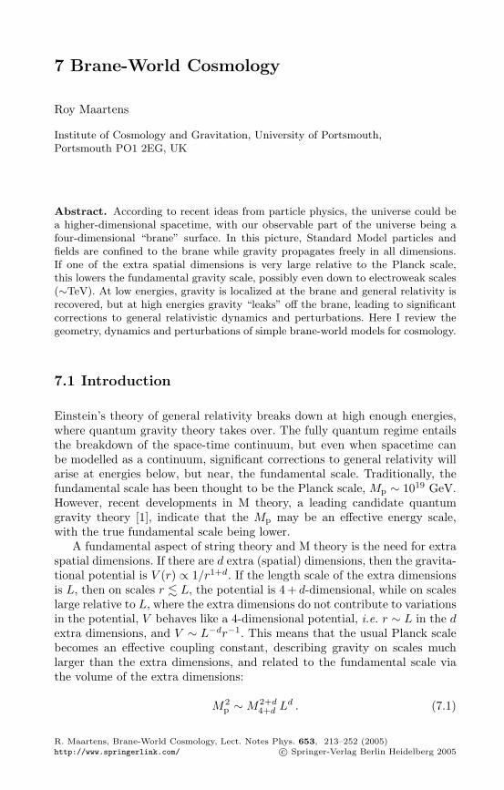
7 Brane-World Cosmology
Roy Maartens
Institute of Cosmology and Gravitation, University of Portsmouth,Portsmouth PO1 2EG, UK
Abstract. According to recent ideas from particle physics, the universe could bea higher-dimensional spacetime, with our observable part of the universe being afour-dimensional “brane” surface. In this picture, Standard Model particles andfields are confined to the brane while gravity propagates freely in all dimensions.If one of the extra spatial dimensions is very large relative to the Planck scale,this lowers the fundamental gravity scale, possibly even down to electroweak scales(∼TeV). At low energies, gravity is localized at the brane and general relativity isrecovered, but at high energies gravity “leaks” off the brane, leading to significantcorrections to general relativistic dynamics and perturbations. Here I review thegeometry, dynamics and perturbations of simple brane-world models for cosmology.
7.1 Introduction
Einstein’s theory of general relativity breaks down at high enough energies,where quantum gravity theory takes over. The fully quantum regime entailsthe breakdown of the space-time continuum, but even when spacetime canbe modelled as a continuum, significant corrections to general relativity willarise at energies below, but near, the fundamental scale. Traditionally, thefundamental scale has been thought to be the Planck scale, Mp ∼ 1019 GeV.However, recent developments in M theory, a leading candidate quantumgravity theory [1], indicate that the Mp may be an effective energy scale,with the true fundamental scale being lower.
A fundamental aspect of string theory and M theory is the need for extraspatial dimensions. If there are d extra (spatial) dimensions, then the gravita-tional potential is V (r) ∝ 1/r1+d. If the length scale of the extra dimensionsis L, then on scales r L, the potential is 4 + d-dimensional, while on scaleslarge relative to L, where the extra dimensions do not contribute to variationsin the potential, V behaves like a 4-dimensional potential, i.e. r ∼ L in the dextra dimensions, and V ∼ L−dr−1. This means that the usual Planck scalebecomes an effective coupling constant, describing gravity on scales muchlarger than the extra dimensions, and related to the fundamental scale viathe volume of the extra dimensions:
M2p ∼M2+d
4+d Ld . (7.1)
R. Maartens, Brane-World Cosmology, Lect. Notes Phys. 653, 213–252 (2005)http://www.springerlink.com/ c© Springer-Verlag Berlin Heidelberg 2005
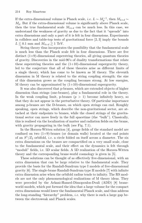
214 Roy Maartens
If the extra-dimensional volume is Planck scale, i.e. L ∼M−1p , then M4+d ∼
Mp. But if the extra-dimensional volume is significantly above Planck scale,then the true fundamental scale M4+d can be much less. In this case, weunderstand the weakness of gravity as due to the fact that it “spreads” intoextra dimensions and only a part of it is felt in four dimensions. Experimentsin colliders and table-top tests of gravitational force [2, 3] imply the boundsL 0.1 mm and M4+d 1 TeV.
String theory thus incorporates the possibility that the fundamental scaleis much less than the Planck scale felt in four dimensions. There are fivedistinct (1+9)-dimensional superstring theories, all giving quantum theoriesof gravity. Discoveries in the mid-90’s of duality transformations that relatethese superstring theories and the (1+10)-dimensional supergravity theory,led to the conjecture that all of these theories arise as different limits ofa single theory, which has come to be known as M theory. The eleventhdimension in M theory is related to the string coupling strength; the sizeof this dimension grows as the coupling becomes strong. At low energies,M theory can be approximated by (1+10)-dimensional supergravity.
It was also discovered that p-branes, which are extended objects of higherdimension than strings (one-branes), play a fundamental role in the theory.In the weak coupling limit, p-branes (p > 1) become infinitely heavy, sothat they do not appear in the perturbative theory. Of particular importanceamong p-branes are the D-branes, on which open strings can end. Roughlyspeaking, open strings, which describe the non-gravitational sector, are at-tached at their endpoints to branes, while the closed strings of the gravita-tional sector can move freely in the full spacetime (the “bulk”). Classically,this is realised via the localization of matter and radiation fields on the brane,with gravity propagating in the bulk (see Fig. 7.1).
In the Horava-Witten solution [4], gauge fields of the standard model areconfined on two (1+9)-branes (or domain walls) located at the end pointsof an S1/Z2 orbifold, i.e. a circle folded on itself across a diameter. The sixextra dimensions on the branes are compactified on a very small scale, closeto the fundamental scale, and their effect on the dynamics is felt through“moduli” fields, i.e. 5D scalar fields. A 5D realization of the Horava-Wittentheory and the corresponding brane-world cosmology is given in [5].
These solutions can be thought of as effectively five-dimensional, with anextra dimension that can be large relative to the fundamental scale. Theyprovide the basis for the Randall-Sundrum type I models of five-dimensionalgravity [6]. The single-brane Randall-Sundrum type II models [7] with infiniteextra dimension arise when the orbifold radius tends to infinity. The RS mod-els are not the only phenomenological realizations of M theory ideas. Theywere preceded by the Arkani-Hamed-Dimopoulos-Dvali (ADD) [8] brane-world models, which put forward the idea that a large volume for the compactextra dimensions would lower the fundamental Planck scale, and thus addressthe long-standing “hierarchy” problem, i.e. why there is such a large gap be-tween the electroweak and Planck scales.

7 Brane-World Cosmology 215
Fig. 7.1. Schematic of confinement of matter to the brane, while gravity propagatesin the bulk (From [2]).
In the ADD models, more than one extra dimension is required for agree-ment with experiments, and there is “democracy” amongst the equivalentextra dimensions, which are furthermore flat. By contrast, the RS modelshave a “preferred” extra dimension, with other extra dimensions treated asignorable (i.e., stabilized except at energies near the fundamental scale). Fur-thermore, this extra dimension is curved or “warped” rather than flat: thebulk is a portion of anti de Sitter (AdS5) spacetime. As in the Horava-Wittensolutions, the RS branes are Z2-symmetric (mirror symmetry), and have atension, which serves to counter the influence of the negative bulk cosmo-logical constant on the brane. This also means that the self-gravity of thebranes is incorporated in the RS models. The novel feature of the RS modelscompared to previous higher-dimensional models is that the observable threedimensions are protected from the large extra dimension (at low energies) bycurvature rather than straightforward compactification.
The RS brane-worlds and their generalizations (to include matter on thebrane, scalar fields in the bulk, etc.) provide phenomenological models thatreflect at least some of the features of M theory, and that bring exciting newgeometric and particle physics ideas into play. The RSII models also providea framework for exploring holographic ideas that have emerged in M theory.This review focuses mainly on RSII-type brane-worlds (see also [9, 10, 11]).
The dilution of gravity via extra dimensions weakens gravity, and it alsoextends the range of graviton modes felt on the brane, beyond the masslessmode of four-dimensional gravity. For simplicity, consider a flat brane withone flat extra dimension, compactified through the identification y ↔ y +
216 Roy Maartens
2πnL, where n = 0, 1, 2, · · · . The perturbative 5D graviton amplitude can beFourier expanded as
f(xa, y) =∑
n
einy/L fn(xa) , (7.2)
where fn are the amplitudes of the KK modes, i.e. the effective 4D modes ofthe the 5D graviton. To see that these KK modes are massive from the braneviewpoint, we start from the 5D wave equation that the massless 5D field fsatisfies (in a suitable gauge):
(5)f = 0 ⇒ f + ∂2yf = 0 . (7.3)
It follows that the KK modes satisfy a 4D Klein-Gordon equation with aneffective 4D mass, mn,
fn = m2n fn , mn =
n
L. (7.4)
The massless mode, f0, is the usual 4D graviton mode. But there is a towerof massive modes, L−1, 2L−1, · · · , which imprint the effect of the 5D gravi-tational field on the 4D brane. Compactness of the extra dimension leads todiscreteness of the spectrum. For an infinite extra dimension, L → ∞, theseparation between the modes disappears and the tower forms a continuousspectrum.
Extra dimensions lead to new scalar and vector degrees of freedom onthe brane. In 5D, the spin-2 graviton is represented by a metric perturbation(5)hAB that is transverse traceless:
(5)hAA = 0 = ∂B
(5)hAB . (7.5)
In a suitable gauge, (5)hAB contains a 3D transverse traceless perturbationhij , a 3D transverse vector perturbation Σi and a scalar perturbation β,each of which satisfies the 5D wave equation (7.3). The 5 degrees of freedom(polarizations) in the 5D graviton are thus split into:a 4D spin-2 graviton hij (2 polarizations); a 4D spin-1 gravi-vector (gravi-photon) Σi (2 polarizations); a 4D spin-0 gravi-scalar β. The standard 4Dgraviton corresponds to the massless zero-mode of hij .
In the general case of d extra dimensions, the number of degrees of freedomin the graviton follows from the irreducible tensor representations of theisometry group as 1
2 (d+ 1)(d+ 4).
7.2 Randall-Sundrum Brane-Worlds
RS brane-worlds do not use compactification to localize gravity at the brane,but the curvature of the bulk. Gravity at low energies is prevented from
7 Brane-World Cosmology 217
leaking into the extra dimension by the gravitational effect of a negative bulkcosmological constant,
Λ5 = − 62
= −6µ2, (7.6)
where is the curvature radius of AdS5:
(5)RABCD = − 12
[(5)gAC
(5)gBD − (5)gAD(5)gBC
], (7.7)
and µ is the corresponding energy scale. In Gaussian normal coordinatesXA = (xµ, y), based on the brane at y = 0, the AdS5 metric takes the form
(5)ds2 = e−2|y|/ηµνdxµdxν + dy2 , (7.8)
with ηµν the Minkowski metric. The exponential warp factor reflects theconfining role of the bulk cosmological constant. The Z2-symmetry aboutthe brane at y = 0 is reflected via the |y| term. In the bulk, this metric is asolution of the 5D Einstein equations,
(5)GAB = −Λ5(5)gAB . (7.9)
The brane is a flat Minkowski spacetime, with self-gravity in the form ofbrane tension. One can also use Poincare coordinates, which bring the metricinto manifestly conformally flat form:
(5)ds2 =2
z2[ηµνdx
µdxν + dz2], z = ey/ . (7.10)
The two RS models are distinguished as follows:
– RSI:There are two branes in RSI [6], at y = 0 and y = L, with Z2-symmetryabout each. The branes have equal and opposite tensions, ±λ, where
λ =3M2
p
4π2. (7.11)
The positive-tension “TeV” (or “hidden”) brane has fundamental scaleM5 ∼ 1 TeV. Standard Model fields are confined on the negative tension“Planck” (or “visible”) brane. Because of the exponential warping factor,the effective scale on the visible brane at y = L is Mp, where
M2p =M3
5 [1 − e−2L/
]. (7.12)
Thus RSI gives a new solution to the hierarchy problem. Because of the fi-nite separation between the branes, the KK spectrum is discrete. In orderto recover 4D general relativity at low energies, a mechanism is requiredto stabilize the inter-brane distance – a scalar field degree of freedomknown as the radion [12].
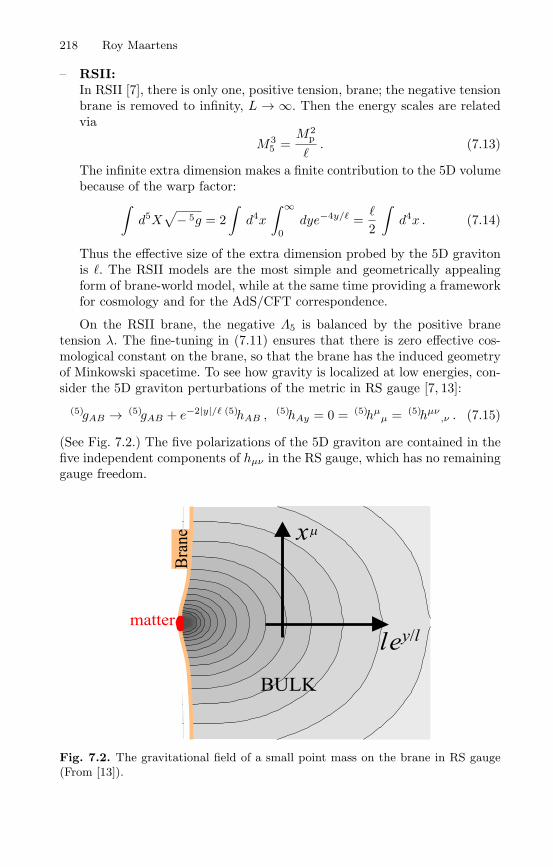
218 Roy Maartens
– RSII:In RSII [7], there is only one, positive tension, brane; the negative tensionbrane is removed to infinity, L → ∞. Then the energy scales are relatedvia
M35 =
M2p
. (7.13)
The infinite extra dimension makes a finite contribution to the 5D volumebecause of the warp factor:
∫d5X
√− 5g = 2
∫d4x
∫ ∞
0dye−4y/ =
2
∫d4x . (7.14)
Thus the effective size of the extra dimension probed by the 5D gravitonis . The RSII models are the most simple and geometrically appealingform of brane-world model, while at the same time providing a frameworkfor cosmology and for the AdS/CFT correspondence.
On the RSII brane, the negative Λ5 is balanced by the positive branetension λ. The fine-tuning in (7.11) ensures that there is zero effective cos-mological constant on the brane, so that the brane has the induced geometryof Minkowski spacetime. To see how gravity is localized at low energies, con-sider the 5D graviton perturbations of the metric in RS gauge [7, 13]:
(5)gAB → (5)gAB + e−2|y|/ (5)hAB ,(5)hAy = 0 = (5)hµ
µ = (5)hµν,ν . (7.15)
(See Fig. 7.2.) The five polarizations of the 5D graviton are contained in thefive independent components of hµν in the RS gauge, which has no remaininggauge freedom.
Fig. 7.2. The gravitational field of a small point mass on the brane in RS gauge(From [13]).

7 Brane-World Cosmology 219
We split the amplitude f of (5)hAB into 3D Fourier modes, and the lin-earized 5D Einstein equations lead to the wave equation (y > 0)
e2y/[f + k2f
]= f ′′ − 4
f ′ . (7.16)
Writingf(t, y) =
∑
m
ϕm(t) fm(y) , (7.17)
the wave equation reduces to
ϕm + (m2 + k2)ϕm = 0 (7.18)
f ′′m − 4
f ′
m + e2y/fm = 0 . (7.19)
The zero mode solution is
ϕ0(t) = A0+e+ikt +A0−e−ikt (7.20)
f0(y) = B0 + C0e4y/ , (7.21)
and the m > 0 solutions are
ϕm(t) = Am+ exp(+i√m2 + k2 t) +Am− exp(−i
√m2 + k2 t) (7.22)
fm(y) = e2y/[BmJ2
(mey/
)+ CmY2
(mey/
)]. (7.23)
The boundary condition follows from the junction conditions, see (7.41)below, and leads to f ′(t, 0) = 0 (since the transverse traceless part of theperturbed energy-momentum tensor on the brane vanishes). Thus
C0 = 0 , Cm = −J1(m)Y1(m)
Bm . (7.24)
The zero mode contribution to the gravitational potential V = 12
(5)h00 givesthe 4D result, V ∝ r−1. The contribution of the massive KK modes sums toa correction of the 4D potential. For r , one obtains
V (r) ≈ GM
r2, (7.25)
which simply reflects the fact that the potential becomes truly 5D on smallscales. For r ,
V (r) ≈ GM
r
(1 +
22
3r2
), (7.26)
which gives the small correction to 4D gravity at low energies from extra-dimensional effects.
Table-top tests of Newton’s laws give 0.1 mm in (7.26). Then by(7.11) and (7.13), this leads to lower limits on the RS brane tension and theRS2 fundamental scale:
λ > (1 TeV)4 , M5 > 105 TeV . (7.27)
220 Roy Maartens
7.3 Covariant Generalization of RS Brane-Worlds
The RS models and the subsequent generalization from a Minkowski braneto a Friedmann-Robertson-Walker (FRW) brane [14, 15, 16], were derived assolutions in particular coordinates of the 5D Einstein equations, together withthe junction conditions at the Z2-symmetric brane. The covariant Shiromizu-Maeda-Sasaki approach [17], is independent of coordinates and applies forgeneral brane and bulk metrics. The basic idea is to use the Gauss-Codazziequations to project the 5D curvature along the brane.
The 5D field equations determine the 5D curvature tensor; in the bulk,they are
(5)GAB = −Λ5(5)gAB + κ2
5(5)TAB , (7.28)
where (5)TAB represents any 5D energy-momentum of the gravitational sector(e.g., dilaton-type scalar fields, form fields).
If y is a Gaussian normal coordinate orthogonal to the brane (at y = 0),then nAdX
A = dy, with nA the unit normal. The 5D metric in terms of theinduced metric on y = const surfaces is
(5)gAB = gAB + nAnB ,(5)ds2 = gµν(xα, y)dxµdxν + dy2 . (7.29)
The extrinsic curvature of y = const. surfaces is
KAB = gAC (5)∇CnB , K[AB] = 0 = KABnB , (7.30)
where square brackets denote anti-symmetrization. The Gauss equation givesthe 4D curvature tensor as
RABCD = (5)REFGH gAEgB
F gCGgD
H + 2KA[CKD]B , (7.31)
and the Codazzi equation determines the change of KAB along y = const:
∇BKB
A − ∇AK = (5)RBC gABnC , (7.32)
where K = KAA.
7.3.1 Field Equations on the Brane
Using (7.28) and (7.31), it follows that
Gµν = −12Λ5gµν +
23κ2
5
[(5)TABgµ
AgνB +
(5)TABn
AnB − 14
(5)T
gµν
]
+KKµν −KµαKαν +
12[KαβKαβ −K2] gµν − Eµν , (7.33)
where (5)T = (5)TAA and
Eµν = (5)CACBD nCnDgµ
AgνB , (7.34)

7 Brane-World Cosmology 221
is the projection of the bulk Weyl tensor, with
EABnB = 0 = E[AB] = EA
A . (7.35)
Evaluating (7.33) as y → ±0, gives the field equations on the brane.First, we need to determineKµν at the brane from the junction conditions.
The total energy-momentum tensor on the brane is
T braneµν = Tµν − λgµν , (7.36)
where Tµν is the energy-momentum tensor of particles and fields confined tothe brane (so that TABn
B = 0). The 5D field equations, including explicitlythe contribution of the brane, are then
(5)GAB = −Λ5(5)gAB + κ2
5
[(5)TAB + T brane
AB δ(y)]. (7.37)
Integrating along the extra dimension and taking the limit, this leads to thejunction conditions at the brane,
g+µν − g−µν = 0 (7.38)
K+µν −K−
µν = −κ25
[T brane
µν − 13T branegµν
], (7.39)
where T brane = gµνT braneµν . The Z2 symmetry means that when you approach
the brane from one side and go through it, you emerge into a bulk that looksthe same, but with the normal reversed, nA → −nA. Then by (7.30)
K−µν = −K+
µν , (7.40)
so that we can use the junction condition (7.39) to determine the extrinsiccurvature on the brane:
Kµν = −12κ2
5
[Tµν +
13
(λ− T ) gµν
], (7.41)
where T = Tµµ, we have dropped the (+) and we evaluate quantities on the
brane by taking the limit y → +0.Finally we arrive at the induced field equations on the brane:
Gµν = −Λgµν + κ2Tµν + 6κ2
λSµν − Eµν + 4
κ2
λFµν , (7.42)
where
κ2 ≡ κ24 =
16λκ4
5 (7.43)
Λ ≡ Λ4 =12[Λ5 + κ2λ
](7.44)
Sµν =112TTµν − 1
4TµαT
αν +
124gµν
[3TαβT
αβ − T 2] (7.45)
Fµν = (5)TABgµAgν
B +[(5)TABn
AnB − 14
(5)T
]gµν . (7.46)

222 Roy Maartens
What about the conservation equations? Using (7.28), (7.32) and (7.41),one obtains
∇νTµν = −2 (5)TABnAgB
µ . (7.47)
Thus in general there is exchange of energy-momentum between the bulk andthe brane. From now on, we will assume that (5)TAB = 0 ⇒ Fµν = 0, sothat
(5)GAB = −Λ5(5)gAB , (bulk) (7.48)
Gµν = −Λgµν + κ2Tµν + 6κ2
λSµν − Eµν , (brane) (7.49)
and one then recovers from (7.47) the standard 4D conservation equations,
∇νTµν = 0 . (7.50)
Then there is no exchange of energy-momentum between the bulk and thebrane; their interaction is purely gravitational. The 4D contracted Bianchiidentities (∇νGµν = 0), applied to (7.42), lead to
∇µEµν =6κ2
λ∇µSµν , (7.51)
which shows qualitatively how (1+3) spacetime variations in the matter-radiation on the brane can source KK modes.
The induced field equations (7.42) show two key modifications to thestandard 4D Einstein field equations arising from extra-dimensional effects:
– Sµν ∼ (Tµν)2 is the high energy correction term, which is negligible forρ λ, but dominant for ρ λ:
|κ2Sµν/λ||κ2Tµν | ∼ |Tµν |
λ∼ ρ
λ. (7.52)
– Eµν , the projection of the bulk Weyl tensor on the brane, encodes correc-tions from 5D graviton effects (the KK modes in the linearized case).
From the brane-observer viewpoint, the energy-momentum corrections inSµν are local, whereas the KK corrections in Eµν are nonlocal, since theyincorporate 5D gravity wave modes. These nonlocal corrections cannot bedetermined purely from data on the brane. In the perturbative analysis ofRSII which leads to the corrections in the gravitational potential, (7.26), theKK modes that generate this correction are responsible for a nonzero Eµν ;this term is what carries the modification to the weak-field field equations.The nine independent components in the trace-free Eµν are reduced to fivedegrees of freedom by (7.51); these arise from the five polarizations of the 5Dgraviton.
Note that the covariant formalism applies also to the two-brane case.In that case, the gravitational influence of the second brane is felt via itscontribution to Eµν .

7 Brane-World Cosmology 223
7.3.2 The Brane Observer’s Viewpoint
The effects of bulk gravity are conveyed, from a brane observer viewpoint, viathe local (Sµν) and nonlocal (Eµν) corrections to Einstein’s equations. (In themore general case, bulk effects on the brane are also carried by Fµν , whichdescribes any 5D fields.) The Eµν term cannot in general be determined fromdata on the brane, and the 5D equations above (or their equivalent) need tobe solved in order to find Eµν .
The general form of the brane energy-momentum tensor for any matterfields (scalar fields, perfect fluids, kinetic gases, dissipative fluids, etc.), in-cluding a combination of different fields, can be covariantly given in terms ofa chosen four-velocity uµ as
Tµν = ρuµuν + phµν + πµν + qµuν + qνuµ . (7.53)
Here ρ and p are the energy density and isotropic pressure, and
hµν = gµν + uµuν , (7.54)
projects into the comoving rest space orthogonal to uµ on the brane. Themomentum density obeys qµ = q〈µ〉, and the anisotropic stress obeys πµν =π〈µν〉, where angled brackets denote the spatially projected, symmetric andtrace-free part:
V〈µ〉 = hµνVν , W〈µν〉 =
[h(µ
αhν)β − 1
3hαβhµν
]Wαβ . (7.55)
In an inertial frame at any point on the brane, we have
uµ = (1,0) , hµν = diag(0, 1, 1, 1) , qµ = (0, qi) , πµ0 = 0 =∑
πii . (7.56)
The tensor Sµν , which carries local bulk effects onto the brane, may thenbe irreducibly decomposed as
Sµν =124[2ρ2 − 3παβπ
αβ]uµuν +
124[2ρ2 + 4ρp+ παβπ
αβ − 4qαqα]hµν
− 112
(ρ+ 2p)πµν + πα〈µπν〉α
+ q〈µqν〉 +13ρq(µuν) − 1
12qαπα(µuν) . (7.57)
This simplifies for a perfect fluid or minimally-coupled scalar field:
Sµν =112ρ [ρuµuν + (ρ+ 2p)hµν ] . (7.58)
The trace free Eµν carries nonlocal bulk effects onto the brane, and con-tributes an effective “dark” radiative energy-momentum on the brane, with

224 Roy Maartens
energy density ρ∗, pressure ρ∗/3, momentum density q∗µ and anisotropic stressπ∗
µν :
− 1κ2 Eµν = ρ∗
(uµuν +
13hµν
)+ q∗µuν + q∗νuµ + π∗
µν . (7.59)
We can think of this as a KK or Weyl “fluid”. The brane “feels” the bulkgravitational field through this effective fluid. More specifically:
– The KK (or Weyl) anisotropic stress π∗µν incorporates the scalar or spin-0
(“Coulomb”), the vector (transverse) or spin-1 (gravimagnetic) and thetensor (transverse traceless) or spin-2 (gravitational wave) 4D modes ofthe spin-2 5D graviton.
– The KK momentum density q∗µ incorporates spin-0 and spin-1 modes, anddefines a velocity v∗
µ of the Weyl fluid relative to uµ via q∗µ = ρ∗v∗µ.
– The KK energy density ρ∗, often called the “dark radiation”, incorporatesthe spin-0 mode.
The RS models have a Minkowski brane in an AdS5 bulk. This bulk is alsocompatible with an FRW brane. However, the most general vacuum bulk witha Friedmann brane is Schwarzschild-anti de Sitter spacetime [18]. It followsfrom the FRW symmetries that q∗µ = 0 = π∗
µν , where ρ∗ = 0 only if the massof the black hole in the bulk is zero. The presence of the bulk black holegenerates via Coulomb effects the dark radiation on the brane.
The brane-world corrections can conveniently be consolidated into an ef-fective total energy density, pressure, momentum density and anisotropicstress.
ρtot = ρ+14λ(2ρ2 − 3πµνπ
µν)
+ ρ∗ (7.60)
ptot = p+14λ(2ρ2 + 4ρp+ πµνπ
µν − 4qµqµ)
+ρ∗
3(7.61)
qtotµ = qµ +12λ
(2ρqµ − 3πµνqν) + q∗µ (7.62)
πtotµν = πµν +
12λ[−(ρ+ 3p)πµν + 3πα〈µπν〉α + 3q〈µqν〉
]+ π∗
µν . (7.63)
These general expressions simplify in the case of a perfect fluid (or minimallycoupled scalar field, or isotropic one-particle distribution function), i.e. forqµ = 0 = πµν :
ρtot = ρ
(1 +
ρ
2λ+ρ∗
ρ
)(7.64)
ptot = p+ρ
2λ(2p+ ρ) +
ρ∗
3(7.65)
qtotµ = q∗µ (7.66)
πtotµν = π∗
µν . (7.67)
7 Brane-World Cosmology 225
Note that nonlocal bulk effects can contribute to effective imperfect fluidterms even when the matter on the brane has perfect fluid form: there is ingeneral an effective momentum density and anisotropic stress induced on thebrane by the 5D graviton.
The effective total equation of state and sound speed follow from (7.64)and (7.65) as
wtot ≡ ptot
ρtot=w + (1 + 2w)ρ/2λ+ ρ∗/3ρ
1 + ρ/2λ+ ρ∗/ρ(7.68)
c2tot ≡ ptot
ρtot=[c2s +
ρ+ pρ+ λ
+4ρ∗
9(ρ+ p)(1 + ρ/λ)
]
[1 +
4ρ∗
3(ρ+ p)(1 + ρ/λ)
]−1
, (7.69)
where w = p/ρ and c2s = p/ρ. At very high energies, i.e., ρ λ, we can gen-erally neglect ρ∗ (e.g., in an inflating cosmology), and the effective equationof state and sound speed are stiffened:
wtot ≈ 2w + 1 , c2tot ≈ c2s + w + 1 . (7.70)
This can have important consequences in the early universe and during gravi-tational collapse. For example, in a very high energy radiation era, w = 1
3 , theeffective cosmological equation of state is ultra-stiff: wtot ≈ 5
3 . In late-stagegravitational collapse of pressureless matter, w = 0, the effective equation ofstate is stiff, wtot ≈ 1, and the effective pressure is nonzero and dynamicallyimportant.
7.3.3 Conservation Equations: Ordinary and “Weyl” Fluids
Conservation of Tµν gives the standard general relativity energy and momen-tum conservation equations:
ρ+Θ(ρ+ p) + Dµqµ + 2Aµqµ + σµνπµν = 0 (7.71)
q〈µ〉 +43Θqµ + Dµp+ (ρ+ p)Aµ
+ Dνπµν +Aνπµν + σµνqν − εµναω
νqα = 0 . (7.72)
In these equations, an overdot denotes uν∇ν , Θ = ∇µuµ is the volume ex-pansion rate of the uµ worldlines, Aµ = uµ = A〈µ〉 is their four-acceleration,σµν = D〈µuν〉 is their shear rate, and ωµ = − 1
2εµαβDαuβ = ω〈µ〉 is theirvorticity rate. On a Friedmann brane,
Aµ = ωµ = σµν = 0 , Θ = 3H , (7.73)
where H = a/a is the Hubble rate. Here Dµ is the spatially projected partof the brane covariant derivative, defined by

226 Roy Maartens
DµFα······β = (∇µF
α······β)⊥ = hµνhα
γ · · ·hβδ∇νF
γ······δ . (7.74)
In a local inertial frame at a point on the brane, with uµ = δµ0, we have:0 = A0 = ω0 = σ0µ = ε0αβ and DµF
α······β = δµiδαj · · · δβk∇iF
j······k, wherei, j, k = 1, 2, 3.
The absence of bulk source terms in the matter conservation equations isa consequence of having Λ5 as the only 5D source in the bulk. For example, ifthere is a bulk scalar field, then there is energy-momentum exchange betweenthe brane and bulk (in addition to the gravitational interaction) [19].
Equation (7.51) may be called the “nonlocal conservation equation forthe Weyl fluid”. Projecting along uµ gives the nonlocal energy conservationequation [20], which is a propagation equation for ρ∗:
ρ∗ +43Θρ∗ + Dµq∗µ + 2Aµq∗µ + σµνπ∗
µν
=14λ
[6πµν πµν + 6(ρ+ p)σµνπµν + 2Θ (2qµqµ + πµνπµν) + 2Aµqνπµν
− 4qµDµρ+ qµDνπµν + πµνDµqν − 2σµνπαµπνα − 2σµνqµqν ] . (7.75)
Projecting into the comoving rest space gives the nonlocal momentum con-servation equation, which is a propagation equation for q∗µ:
q∗〈µ〉 +43Θq∗µ +
13Dµρ
∗ +43ρ∗Aµ + Dνπ∗
µν +Aνπ∗µν + σµ
νq∗ν − εµναωνq∗α
=14λ[−4(ρ+ p)Dµρ+ 6(ρ+ p)Dνπµν + qν π〈µν〉 + πµ
νDν(2ρ+ 5p)
− 23παβ (Dµπαβ + 3Dαπβµ) − 3πµαDβπ
αβ +283qνDµqν
+ 4ρAνπµν − 3πµαAβπαβ +
83Aµπ
αβπαβ − πµασαβqβ
+ σµαπαβqβ + πµνε
ναβωαqβ − εµαβωαπβνqν + 4(ρ+ p)Θqµ
+ 6qµAνqν +143Aµq
νqν + 4qµσαβπαβ
]. (7.76)
The (1+3)-covariant decomposition shows two key features:
– inhomogeneous and anisotropic effects from the 4D matter-radiation dis-tribution on the brane are a source for the 5D Weyl tensor, which nonlo-cally “backreacts” on the brane via its projection Eµν ;
– there are evolution equations for the dark radiative (nonlocal, Weyl) en-ergy (ρ∗) and momentum (q∗µ) densities (carrying scalar and vector modesfrom bulk gravitons), but there is no evolution equation for the dark ra-diative anisotropic stress (π∗
µν) (carrying tensor, as well as scalar andvector, modes), which arises in both evolution equations.
In particular cases, the Weyl anisotropic stress π∗µν may drop out of the
nonlocal conservation equations, i.e. when we can neglect σµνπ∗µν , Dνπ∗
µν

7 Brane-World Cosmology 227
and Aνπ∗µν . This is the case when we consider linearized perturbations about
an FRW background (which remove the first and last of these terms) andfurther when we can neglect gradient terms on large scales (which removesthe second term) [20]. But in general, on small scales in cosmology, andespecially in astrophysical contexts, the π∗
µν terms cannot be neglected.All of the matter source terms on the right of these two equations, except
for the first term on the right of (7.76), are imperfect fluid terms, and most ofthese terms are quadratic in the imperfect quantities qµ and πµν . For a singleperfect fluid or scalar field, only the Dµρ term on the right of (7.76) survives,but in realistic cosmological and astrophysical models, further terms willsurvive. For example, terms linear in πµν will carry the photon quadrupolein cosmology or the shear viscous stress in stellar models. If there are twofluids (even if both fluids are perfect), then there will be a relative velocity vµgenerating a momentum density qµ = ρvµ, which will serve to source nonlocaleffects.
In general, the four independent equations in (7.75) and (7.76) constrainfour of the nine independent components of Eµν on the brane. What is miss-ing, is an evolution equation for π∗
µν (which has up to five independent compo-nents). Thus in general, the projection of the five-dimensional field equationsonto the brane does not lead to a closed system, as expected, since there arebulk degrees of freedom whose impact on the brane cannot be predicted bybrane observers. The Weyl or KK anisotropic stress π∗
µν encodes the nonlo-cality.
In special cases the missing equation does not matter. For example, ifπ∗
µν = 0 by symmetry, as in the case of an FRW brane, then the evolution ofEµν is determined by (7.75) and (7.76). However, small perturbations of thisspecial case will immediately restore the problem of missing information.
If the matter on the brane has a perfect-fluid energy-momentum tensor,the local conservation equations (7.71) and (7.72) reduce to
ρ+Θ(ρ+ p) = 0 (7.77)Dµp+ (ρ+ p)Aµ = 0 , (7.78)
while the nonlocal conservation equations (7.75) and (7.76) reduce to
ρ∗ +43Θρ∗ + Dµq∗µ = 0 (7.79)
q∗〈µ〉 +43Θq∗µ +
13Dµρ
∗ +43ρ∗Aµ + Dνπ∗
µν = − (ρ+ p)λ
Dµρ , (7.80)
where we have also linearized about an FRW background.

228 Roy Maartens
7.4 Brane-World Cosmology: Dynamics
In the FRW case, (7.80) is trivially satisfied, while (7.79) becomes
ρ∗ + 4Hρ∗ = 0 . (7.81)
This equation has the dark radiation solution
ρ∗ = ρ∗0
(a0a
)4. (7.82)
In natural static coordinates, the Schwarzschild-AdS5 metric for an FRWbrane-world is
(5)ds2 = −F (R)dT 2 +dR2
F (R)+R2
(dr2
1 −Kr2 + r2dΩ2)
(7.83)
F (R) = K +R2
2− m
R2 , (7.84)
where K = 0,±1 is the FRW curvature index and m is the mass parameterof the black hole at R = 0 (note that the 5D gravitational potential has R−2
behaviour). The bulk black hole gives rise to dark radiation on the brane viaits Coulomb effect. The FRW brane moves radially along the fifth dimension,with R = a(T ), where a is the FRW scale factor, and the junction conditionsdetermine the velocity via the Friedmann equation for a [18]. Thus one caninterpret the expansion of the universe as motion of the brane through thestatic bulk. In the special case m = 0 and da/dT = 0, the brane is fixed andhas Minkowski geometry, i.e. the original RSII brane-world is recovered, indifferent coordinates.
The velocity of the brane is coordinate-dependent, and can be set to zero.We can use Gaussian normal coordinates, in which the brane is fixed but thebulk metric is not manifestly static [14]:
(5)ds2 = −N2(t, y)dt2 +A2(t, y)[
dr2
1 −Kr2 + r2dΩ2]
+ dy2 . (7.85)
Here a(t) = A(t, 0) is the scale factor on the FRW brane at y = 0, and t maybe chosen as proper time on the brane, so that N(t, 0) = 1. In the case wherethere is no bulk black hole (m = 0), the metric functions are
N =A(t, y)a(t)
(7.86)
A = a(t)[cosh
(y
)−
1 +ρ(t)λ
sinh
( |y|
)]. (7.87)
Again, the junction conditions determine the Friedmann equation. The ex-trinsic curvature at the brane is
7 Brane-World Cosmology 229
Kµν = diag
(N ′
N,A′
A,A′
A,A′
A
)
brane. (7.88)
Then, by (7.41),
N ′
N
∣∣∣brane
=κ2
5
6(2ρ+ 3p− λ) (7.89)
A′
A
∣∣∣brane
= −κ25
6(ρ+ λ) . (7.90)
The field equations yield the first integral [14]
(AA′)2 − A2
N2 A2 +
Λ5
6A4 +m = 0 , (7.91)
where m is constant. Evaluating this at the brane, using (7.90), gives themodified Friedmann equation
H2 =κ2
3ρ(1 +
ρ
2λ
)+m
a4+
13Λ− K
a2. (7.92)
By (7.82),
m =κ2
3ρ∗0a
40 . (7.93)
The Friedmann and matter energy conservation equations yield
H = −κ2
2(ρ+ p)
(1 +
ρ
λ
)− 2
m
a4+K
a2. (7.94)
When the bulk black hole mass vanishes, the bulk geometry reduces toAdS5 and ρ∗ = 0. In order to avoid a naked singularity, we assume that theblack hole mass is non-negative, so that ρ∗
0 ≥ 0. [By (7.84), it is possible toavoid a naked singularity with negative m when K = −1, provided |m| ≤2/4.] This additional effective relativistic degree of freedom is constrainedby nucleosynthesis and CMB observations to be no more than ∼5% of theradiation energy density [21, 22]:
ρ∗
ρrad
∣∣∣∣nuc
. 0.05 (7.95)
The other modification to the Hubble rate is via the high energy correctionρ/λ. In order to recover the observational successes of general relativity, thehigh energy regime where significant deviations occur must take place beforenucleosynthesis, i.e., cosmological observations impose the lower limit
λ > (1 MeV)4 ⇒ M5 > 104 GeV . (7.96)
This is much weaker than the limit imposed by table-top experiments, (7.27).Since ρ2/λ decays as a−8 during the radiation era, it will rapidly becomenegligible after the end of the high energy regime, ρ = λ.
230 Roy Maartens
If ρ∗ = 0 and K = 0 = Λ, then the exact solution of the Friedmannequations for w = p/ρ = const. is [14]
a = const [t(t+ tλ)]1/3(w+1) , tλ =Mp√
3πλ(1 + w) (1 + w)−110−9 sec ,
(7.97)where w > −1. If ρ∗ = 0 (but K = 0 = Λ), then the solution for the radiationera (w = 1
3 ) is
a = const [t(t+ tλ)]1/4 , tλ =√
3Mp
4√πλ (1 + ρ∗/ρ)
. (7.98)
For t tλ we recover from (7.97) and (7.98) the standard behaviour, a ∝t2/3(w+1), whereas for t tλ, we have the very different behaviour of thehigh energy regime,
ρ λ ⇒ µ ∝ t1/3(w+1) . (7.99)
When w = −1 we have ρ = ρ0 from the conservation equation. If K =0 = Λ, we recover the de Sitter solution for ρ∗ = 0 and an asymptotically deSitter solution for ρ∗ > 0:
ρ∗ = 0 : a = a0 exp[H0(t− t0)] , H0 = κ√ρ03
(1 +
ρ02λ
)(7.100)
ρ∗ > 0 : a2 =√m
H0sinh[2H0(t− t0)] . (7.101)
7.5 Brane-World Inflation
In RSII-type brane-worlds, where the bulk has only a vacuum energy, inflationon the brane must be driven by a 4D scalar field trapped on the brane. Inmore general brane-worlds, where the bulk contains a 5D scalar field, it ispossible that the 5D field induces inflation on the brane via its effectiveprojection [23].
More exotic possibilities arise from the interaction between two branes,including possible collision, which is mediated by a 5D scalar field and whichcan induce either inflation [24] or a hot big-bang radiation era, as in the“ekpyrotic” or cyclic scenario [25]. Here we discuss the simplest case of a 4Dscalar field φ with potential V (φ).
High energy brane-world modifications to the dynamics of inflation on thebrane have been investigated [26, 27]. Essentially, the high energy correctionsprovide increased Hubble damping, since ρ λ impliesH is larger for a givenenergy than in 4D general relativity. This makes slow-roll inflation possibleeven for potentials that would be too steep in standard cosmology [26, 28, 29].
The field satisfies the Klein-Gordon equation
7 Brane-World Cosmology 231
φ+ 3Hφ+ V ′(φ) = 0 . (7.102)
In 4D general relativity, the condition for inflation, a > 0, is φ2 < V (φ), i.e.,p < − 1
3ρ, where ρ = 12 φ
2 + V and p = 12 φ
2 − V . The modified Friedmannequation leads to a stronger condition for inflation: using (7.92), with m =0 = Λ = K, and (7.102), we find that
a > 0 ⇒ w < −13
[1 + 2ρ/λ1 + ρ/λ
], (7.103)
where the square brackets enclose the brane correction to the general relativ-ity result. As ρ/λ/ → 0, the 4D result w < − 1
3 is recovered, but for ρ > λ, wmust be more negative for inflation. In the very high energy limit ρ/λ → ∞,we have w < − 2
3 . When the only matter in the universe is a self-interactingscalar field, the condition for inflation becomes
φ2 − V +
[12 φ
2 + Vλ
(54φ2 − 1
2V
)]
< 0 , (7.104)
which reduces to φ2 < V when ρφ = 12 φ
2 + V λ.In the the slow-roll approximation,
H2 ≈ κ2
3V
[1 +
V
2λ
](7.105)
φ ≈ − V ′
3H. (7.106)
The brane-world correction term V/λ in (7.105) serves to enhance the Hubblerate for a given potential energy, relative to general relativity. Thus there isenhanced Hubble ‘friction’ in (7.106), and brane-world effects will reinforceslow-roll at the same potential energy. We can see this by defining slow-rollparameters that reduce to the standard parameters in the low-energy limit:
ε ≡ − H
H2 =M2
p
16π
(V ′
V
)2 [ 1 + V/λ(1 + V/2λ)2
](7.107)
η ≡ − φ
Hφ=M2
p
8π
(V ′′
V
)[1
1 + V/2λ
]. (7.108)
Self-consistency of the slow-roll approximation then requires ε, |η| 1. Atlow energies, V λ, the slow-roll parameters reduce to the standard form.However at high energies, V λ, the extra contribution to the Hubbleexpansion helps damp the rolling of the scalar field and the new factors insquare brackets become ≈ λ/V :
ε ≈ εgr[4λV
], η ≈ ηgr
[2λV
], (7.109)

232 Roy Maartens
where εgr, ηgr are the standard general relativity slow-roll parameters. In par-ticular, this means that steep potentials which do not give inflation in generalrelativity, can inflate the brane-world at high energy and then naturally stopinflating when V drops below λ. These models can be constrained becausethey typically end inflation in a kinetic-dominated regime and thus generate ablue spectrum of gravitational waves, which can disturb nucleosynthesis [28].They also allow for the novel possibility that the inflaton could act as darkmatter or quintessence at low energies [28, 30].
The number of e-folds during inflation, N =∫Hdt, is, in the slow-roll
approximation,
N ≈ − 8πM2
p
∫ φf
φi
V
V ′
[1 +
V
2λ
]dφ . (7.110)
Brane-world effects at high energies increase the Hubble rate by a factorV/2λ, yielding more inflation between any two values of φ for a given po-tential. Thus we can obtain a given number of e-folds for a smaller initialinflaton value φi. For V λ, (7.110) becomes
N ≈ −128π3
3M65
∫ φf
φi
V 2
V ′ dφ . (7.111)
The key test of any modified gravity theory during inflation, will be thespectrum of perturbations produced due to quantum fluctuations of the fieldsabout their homogeneous background values. We will discuss brane-worldcosmological perturbations in the next section. In general, perturbations onthe brane are coupled to bulk metric perturbations, and the problem is verycomplicated. However on large scales on the brane, the density and curvatureperturbations decouple from the bulk metric perturbations [20, 21]. Thus weare justified in neglecting the nonlocal effects carried by Eµν when computingthe density perturbations.
To quantify the amplitude of scalar (density) perturbations we evaluatethe usual gauge invariant quantity
ζ ≡ R − H
ρδρ , (7.112)
which reduces to the curvature perturbation, R, on uniform density hyper-surfaces (δρ = 0). This is conserved on large scales for purely adiabaticperturbations, as a consequence of energy conservation (independently of thefield equations) [31]. The curvature perturbation on uniform density hyper-surfaces is given in terms of the scalar field fluctuations on spatially flathypersurfaces, δφ, by
ζ = Hδφ
φ. (7.113)
The field fluctuations at Hubble crossing (k = aH) in the slow-roll limit aregiven by 〈δφ2〉 ≈ (H/2π)2, a result for a massless field in de Sitter space that

7 Brane-World Cosmology 233
is also independent of the gravity theory [31]. For a single scalar field theperturbations are adiabatic and hence the curvature perturbation ζ can berelated to the density perturbations when modes re-enter the Hubble scaleduring the matter dominated era which is given by A2
s = 4〈ζ2〉/25. Using theslow-roll equations and (7.113), this gives
A2s ≈
(512π75M6
p
V 3
V ′2
)[2λ+ V
2λ
]3∣∣∣∣∣k=aH
. (7.114)
Thus the amplitude of scalar perturbations is increased relative to the stan-dard result at a fixed value of φ for a given potential.
The scale-dependence of the perturbations is described by the spectraltilt
ns − 1 ≡ d lnA2s
d ln k≈ −6ε+ 2η , (7.115)
where the slow-roll parameters are given in (7.107) and (7.108). Becausethese slow-roll parameters are both suppressed by an extra factor λ/V athigh energies, we see that the spectral index is driven towards the Harrison-Zel’dovich spectrum, ns → 1, as V/λ → ∞; however, this does not necessarilymean that the brane-world case is closer to scale-invariance than the generalrelativity case.
In comparing the high energy brane-world case to the standard 4D case,we implicitly require the same potential energy. However, precisely because ofthe high energy effects, large scale perturbations will be generated at differentvalues of V than in the standard case, specifically at lower values of V , closerto the reheating minimum. Thus there are two competing effects, and itturns out that the shape of the potential determines which is the dominanteffect [32]. For the quadratic potential, the lower location on V dominates,and the spectral tilt is slightly further from scale invariance than in thestandard case. The same holds for the quartic potential. Data from WMAPand 2dF can be used to constrain inflationary models via their deviation fromscale invariance, and the high energy brane-world versions of the quadraticand quartic potentials are thus under more pressure from data than theirstandard counterparts [32].
Other perturbation modes are also generated in inflation:
– High energy inflation on the brane also generates a zero mode (4D gravi-ton mode) of tensor perturbations, and stretches it to super-Hubble scales,as will be discussed below. This zero mode has the same qualitative fea-tures as in general relativity, remaining frozen at constant amplitude whilebeyond the Hubble horizon. Its amplitude is enhanced at high energies,although the enhancement is much less than for scalar perturbations [33]:

234 Roy Maartens
A2t ≈
(32V
75M2p
)[3V 2
4λ2
](7.116)
A2t
A2s
≈(M2
p
16πV ′2
V 2
)[6λV
]. (7.117)
Equation (7.117) means that brane-world effects suppress the large scaletensor contribution to CMB anisotropies. The tensor spectral index athigh energy has a smaller magnitude than in general relativity,
nt = −3ε , (7.118)
but remarkably the same consistency relation as in general relativityholds [29]:
nt = −2A2
t
A2s. (7.119)
The massive KK modes of tensor perturbations remain in the vacuumstate during slow-roll inflation [33, 34]. The evolution of the super-Hubblezero mode is the same as in general relativity, so that high energy brane-world effects in the early universe serve only to rescale the amplitude.However, when the zero mode re-enters the Hubble horizon, massive KKmodes can be excited.
– Vector perturbations in the bulk metric can support vector metric per-turbations on the brane, even in the absence of matter perturbations.However, there is no normalizable zero mode, and the massive KK modesstay in the vacuum state during brane-world inflation [35]. Therefore, asin general relativity, we can neglect vector perturbations in inflationarycosmology.
7.6 Brane-World Cosmology: Perturbations
The background dynamics of brane-world cosmology are simple because theFRW symmetries simplify the bulk and rule out nonlocal effects. But pertur-bations on the brane in general release the nonlocal KK modes. Then the 5Dbulk perturbation equations must be solved in order to solve for perturba-tions on the brane. These 5D equations are partial differential equations forthe three-Fourier modes, with complicated initial and boundary conditions.
The theory of gauge invariant perturbations in brane-world cosmology hasbeen extensively investigated and developed (see references given in the re-views [9, 10, 11]) and is qualitatively well understood (for a general review oncosmological perturbations see the review article by R. Durrer). The key re-maining task is integration of the coupled brane-bulk perturbation equations.Special cases have been solved, where these equations effectively decouple, asin the previous section, and approximation schemes have recently been devel-oped [36, 37, 38, 39, 40] for the more general cases where the coupled system
7 Brane-World Cosmology 235
must be solved. From the brane viewpoint, the bulk effects, i.e. the highenergy corrections and the KK modes, act as source terms for the brane per-turbation equations. At the same time, perturbations of matter on the branecan generate KK modes (i.e. emit 5D gravitons into the bulk) which propa-gate in the bulk and can subsequently interact with the brane. This nonlocalinteraction amongst the perturbations is at the core of the complexity of theproblem. It can be elegantly expressed via integro-differential equations [41],which take the form (assuming no incoming 5D gravitational waves)
Ak(t) =∫dt′ G(t, t′)Bk(t′) , (7.120)
where G is the bulk retarded Green’s function evaluated on the brane, andAk, Bk are made up of brane metric and matter perturbations and their(brane) derivatives, and include high energy corrections to the backgrounddynamics. Solving for the bulk Green’s function which then determines G, isthe core of the 5D problem.
We can isolate the KK anisotropic stress π∗µν as the term that must be
determined from 5D equations. Once π∗µν is determined in this way, the per-
turbation equations on the brane form a closed system. The solution will beof the form, expressed in Fourier modes:
π∗k(t) ∝
∫dt′ G(t, t′)Fk(t′) , (7.121)
where the functional Fk will be determined by the brane perturbation quanti-ties and their derivatives. It is known in the case of a Minkowski background,but not in the cosmological case.
7.6.1 Metric-Based Perturbations
A review of this approach is given in [42]. In an arbitrary gauge, and for aflat FRW background, the perturbed metric has the form
δ (5)gAB =
−2N2ψ A2(∂iB − Si) Nα
A2(∂jB − Sj) A2 2Rδij + 2∂i∂jC A2(∂iβ − χi)+2∂(iFj) + fij
Nα A2(∂jβ − χj) 2ν
, (7.122)
where the background metric functions A,N are given by (7.86) and (7.87).The scalars ψ,R, C, α, β, ν represent scalar perturbations. The vectors Si, Fi
and χi are transverse, so that they represent 3D vector perturbations, andthe tensor fij is transverse traceless, representing 3D tensor perturbations.
In the Gaussian normal gauge, the brane coordinate-position remainsfixed under perturbation,

236 Roy Maartens
(5)ds2 =[g(0)µν (x, y) + δgµν(x, y)
]dxµdxν + dy2 , (7.123)
where g(0)µν is the background metric, (7.85), so that
α = β = ν = χi = 0 . (7.124)
In the 5D longitudinal gauge,
−B + C = 0 = −β + C′ . (7.125)
In this gauge, and for an AdS5 background, the metric perturbation quantitiescan all be expressed in terms of a “master variable” [41] Ω which obeys awave equation. In the case of scalar perturbations, we have for example,
R =1
6A
(Ω′′ − 1
N2 Ω − Λ5
3Ω
), (7.126)
with similar expressions for the other quantities. All of the metric perturba-tion quantities are determined once solution is found for the wave equation
(1
NA3 Ω
)·+(Λ5
6+k2
A2
)N
A3 Ω =(N
A3 Ω′)′. (7.127)
The junction conditions (7.41) relate the off-brane derivatives of metricperturbations to the matter perturbations:
∂y δgµν = −κ25
[δTµν +
13
λ− T (0)
δgµν − 1
3g(0)µν δT
], (7.128)
where
δT 00 = −δρ , δT 0
i = a2qi (7.129)δT i
j = δp δij + δπij . (7.130)
For scalar perturbations in the Gaussian normal gauge, this gives
∂yψ(x, 0) =κ2
5
6(2δρ+ 3δp) (7.131)
∂yB(x, 0) = κ25δp (7.132)
∂yC(x, 0) = −κ25
2δπ (7.133)
∂yR(x, 0) = −κ25
6δρ− ∂i∂
i C(x, 0) , (7.134)
where δπ is the scalar potential for the matter anisotropic stress,
δπij = ∂i∂jδπ − 13δij ∂k∂
kδπ . (7.135)
7 Brane-World Cosmology 237
The perturbed nonlocal (dark radiation) stress tensor on the brane is givenby
δE00 = κ2δρ∗ , δE0
i = −κ2a2q∗i (7.136)
δE ij = −κ
2
3δρ∗ δij + δπ∗i
j . (7.137)
The evolution of the bulk metric perturbations is determined by the per-turbed 5D field equations in the vacuum bulk,
δ (5)GAB = 0 . (7.138)
Then the matter perturbations on the brane enter via the perturbed junctionconditions, (7.128).
For example, for scalar perturbations in Gaussian normal gauge,
δ (5)Gyi = ∂i
−ψ′ +
(A′
A− N ′
N
)ψ − 2R′
− A2
2N2
[
B′ +
(
5A
A− N
N
)
B′]
. (7.139)
For tensor perturbations (in any gauge), the only nonzero components of theperturbed Einstein tensor are
δ (5)Gij = −1
2
− 1N2 f
ij + f ′′i
j − k2
A2 fij
+1N2
(N
N− 3
A
A
)
f ij +(N ′
N+ 3
A′
A
)f ′i
j
. (7.140)
7.6.2 Curvature Perturbations and the Sachs–Wolfe Effect
The curvature perturbation R on uniform density surfaces is defined in(7.122). The associated gauge-invariant quantity
ζ = R +δρ
3(ρ+ p), (7.141)
may be defined for matter on the brane. Similarly, for the Weyl “fluid” ifρ∗ = 0 in the background, the curvature perturbation on hypersurfaces ofuniform dark energy density is
ζ∗ = R +δρ∗
4ρ∗ . (7.142)
On large scales, the perturbed dark energy conservation equation is [21]
238 Roy Maartens
(δρ∗)· + 4Hδρ∗ + 4ρ∗R = 0 , (7.143)
which leads toζ∗ = 0 . (7.144)
For adiabatic matter perturbations, by the perturbed matter energy conser-vation equation,
(δρ)· + 3H(δρ+ δp) + 3(ρ+ p)R = 0 (7.145)
we findζ = 0 . (7.146)
This is independent of brane-world modifications to the field equations, sinceit depends on energy conservation only. For the total, effective fluid, thecurvature perturbation is defined as follows [21]: if ρ∗ = 0 in the background,
ζtot = ζ +[
4ρ∗
3(ρ+ p)(1 + ρ/λ) + 4ρ∗
](ζ∗ − ζ) , (7.147)
and if ρ∗ = 0 in the background,
ζ tot = ζ +δρ∗
3(ρ+ p)(1 + ρ/λ)(7.148)
δρ∗ =δC∗
a4, (7.149)
where δC∗ is a constant. It follows that the curvature perturbations on largescales, like the density perturbations, can be found on the brane withoutsolving for the bulk metric perturbations.
Note that ζ tot = 0 even for adiabatic matter perturbations; for example,if ρ∗ = 0 in the background,
ζ tot = H(c2tot − 1
3
)δρ∗
(ρ+ p)(1 + ρ/λ). (7.150)
The KK effects on the brane contribute a non-adiabatic mode, althoughζ tot → 0 at low energies.
Although the density and curvature perturbations can be found on super-Hubble scales, the Sachs-Wolfe effect requires π∗
µν in order to translate fromdensity/ curvature to metric perturbations. In the 4D longitudinal gauge ofthe metric perturbation formalism, the gauge invariant curvature and metricperturbations on large scales are related by
ζtot = R − H
H
(RH
− ψ)
(7.151)
R + ψ = −κ2a2δπ∗ , (7.152)
7 Brane-World Cosmology 239
where the radiation anisotropic stress on large scales is neglected, as in generalrelativity, and δπ∗ is the scalar potential for π∗
µν (equivalent to the covariantquantity Π). In 4D general relativity, the right hand side of (7.152) is zero.The (non-integrated) Sachs-Wolfe formula has the same form as in generalrelativity:
δT
T
∣∣∣now
= (ζrad + ψ − R)|dec . (7.153)
The brane-world corrections to the general relativistic Sachs-Wolfe effect arethen given by [21]
δT
T=(δT
T
)
gr− 8
3
(ρradρcdm
)S∗ − κ2a2δπ∗ +
2κ2
a5/2
∫da a7/2 δπ∗ , (7.154)
where S∗ is the KK entropy perturbation (determined by δρ∗). The KK termδπ∗ cannot be determined by the 4D brane equations, so that δT/T cannot beevaluated on large scales without solving the 5D equations. Equation (7.154)has been generalized to the two-brane case, in which the radion makes acontribution to the Sachs-Wolfe effect [43].
The presence of the KK (Weyl, dark) component has essentially two pos-sible effects.
– A contribution from the KK entropy perturbation S∗ that is similar toan extra isocurvature contribution.
– The KK anisotropic stress δπ∗ also contributes to the CMB anisotropies.In the absence of anisotropic stresses, the curvature perturbation ζtot issufficient to determine the metric perturbation R and hence the largeangle CMB anisotropies, via (7.151), (7.152) and (7.153). However bulkgravitons can also generate anisotropic stresses which, although they donot affect the large-scale curvature perturbation ζtot, can affect the rela-tion between ζtot, R and ψ, and hence can affect the CMB anisotropiesat large angles.
7.7 Gravitational Wave Perturbations
The tensor perturbations are given by (7.122), i.e. (for a flat backgroundbrane),
(5)ds2 = −N2(t, y)dt2 +A2(t, y) [δij + fij ] dxidxj + dy2 . (7.155)
The transverse traceless fij satisfies (7.140), which implies, on splitting fij
into Fourier modes with amplitude f(t, y),
1N2
[
f +
(
3A
A− N
N
)
f
]
+k2
A2 f = f ′′ +(
3A′
A+N ′
N
)f ′ . (7.156)

240 Roy Maartens
By the transverse traceless part of (7.128), the boundary condition is
f ′ij
∣∣brane = πij , (7.157)
where πij is the tensor part of the anisotropic stress of matter-radiation onthe brane.
The wave equation (7.156) cannot be solved analytically except if thebackground metric functions are separable, and this only happens for max-imally symmetric branes, i.e. branes with constant Hubble rate H0. Thisincludes the RS case H0 = 0, already treated above. The cosmologically rel-evant case is the de Sitter brane, H0 > 0. We can calculate the spectrum ofgravitational waves generated during brane inflation [33, 34, 44, 45], if we ap-proximate slow-roll inflation by a succession of de Sitter phases. The metricfor a de Sitter brane, dS4, in AdS5 is given by (7.85)–(7.87) with
N(t, y) = n(y) , A(t, y) = a(t)n(y) (7.158)
n(y) = coshµy −(1 +
ρ0λ
)sinhµ|y| (7.159)
a(t) = a0 expH0(t− t0) , H20 =
κ2
3ρ0
(1 +
ρ02λ
), (7.160)
where µ = −1.The linearized wave equation (7.156) is separable. As before, we separate
the amplitude as f =∑ϕm(t)fm(y) where m is the 4D mass, and this leads
to:
ϕm + 3H0ϕm +[m2 +
k2
a2
]ϕm = 0 (7.161)
f ′′m + 4
n′
nf ′
m +m2
n2 fm = 0 . (7.162)
The general solutions for m > 0 are
ϕm(t) = exp(
−32H0t
)Bν
(k
H0e−H0t
)(7.163)
fm(y) = n(y)−3/2Lν3/2
(√
1 +µ2
H20n(y)2
)
, (7.164)
where Bν is a linear combination of Bessel functions, Lν3/2 is a linear combi-
nation of associated Legendre functions, and
ν = i
√m2
H20
− 94. (7.165)
It is more useful to reformulate (7.162) as a Schrodinger-type equation,
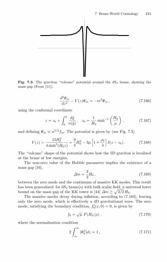
7 Brane-World Cosmology 241
Fig. 7.3. The graviton “volcano” potential around the dS4 brane, showing themass gap (From [11]).
d2Ψm
dz2− V (z)Ψm = −m2Ψm , (7.166)
using the conformal coordinate
z = zb +∫ y
0
dy
n(y), zb =
1H0
sinh−1(H0
µ
), (7.167)
and defining Ψm ≡ n3/2fm. The potential is given by (see Fig. 7.3)
V (z) =15H2
0
4 sinh2(H0z)+
94H2
0 − 3µ[1 +
ρ0λ
]δ(z − zb) . (7.168)
The “volcano” shape of the potential shows how the 5D graviton is localizedat the brane at low energies.
The non-zero value of the Hubble parameter implies the existence of amass gap [16],
∆m =32H0 , (7.169)
between the zero mode and the continuum of massive KK modes. This resulthas been generalized: for dS4 brane(s) with bulk scalar field, a universal lowerbound on the mass gap of the KK tower is [44] ∆m ≥√3/2H0.
The massive modes decay during inflation, according to (7.163), leavingonly the zero mode, which is effectively a 4D gravitational wave. The zeromode, satisfying the boundary condition, f ′
0(x, 0) = 0, is given by
f0 =√µ F (H0/µ) , (7.170)
where the normalization condition
2∫ ∞
zb
|Ψ20 |dz = 1 , (7.171)

242 Roy Maartens
implies that the function F is given by
F (x) =
√
1 + x2 − x2 ln
[1x
+
√
1 +1x2
]−1/2
. (7.172)
At low energies (H0 µ), we recover the general relativity amplitude: F → 1.At high energies, the amplitude is considerably enhanced:
H0 µ ⇒ F ≈√
3H0
2µ. (7.173)
The factor F determines the modification of the gravitational wave amplituderelative to the standard 4D result:
A2t =
[8M2
p
(H0
2π
)2]
F 2(H0/µ). (7.174)
This enhanced zero mode produced by brane inflation remains frozenoutside the Hubble radius, as in general relativity, but when it re-enters theHubble radius during radiation or matter domination, it will no longer beseparated from the massive modes, since H will not be constant. Instead,massive modes will be excited during re-entry. In other words, energy willbe lost from the zero mode as 5D gravitons are emitted into the bulk, i.e.as massive modes are produced on the brane. Self-consistent low energy ap-proximations to compute this effect are developed in [39, 40].
At zero order, the low-energy approximation is based on the following.In the radiation era, at low energy, the background metric functions obeyA(t, y) → a(t)e−µy and N(t, y) → e−µy. To lowest order, the wave equa-tion therefore separates, and the mode functions can be found analytically.The massive modes in the bulk, fm(y), are the same as for a Minkowskibrane. The massive modes decay on super-Hubble scales, unlike the zero-mode. Expanding the wave equation in ρ0/λ, one arrives at the first order,where mode-mixing arises. The numerical integration of the equations [39]confirms the effect of massive mode generation and consequent damping ofthe zero-mode, as shown in Fig. 7.4.
7.8 Brane-World CMB Anisotropies
Recently, the anisotropies in the CMB for RS-type brane-world cosmologieshave been calculated using a low-energy approximation [37] (for a reviewon CMB anisotropies see A. Challinor’s contribution). The basic idea of thelow-energy approximation [36] is to use a gradient expansion to exploit thefact that, during most of the history of the universe, the curvature scale on
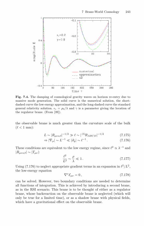
7 Brane-World Cosmology 243
Fig. 7.4. The damping of cosmological gravity waves on horizon re-entry due tomassive mode generation. The solid curve is the numerical solution, the short-dashed curve the low-energy approximation, and the long-dashed curve the standardgeneral relativity solution. ε∗ = ρ0/λ and γ is a parameter giving the location ofthe regulator brane. (From [39]).
the observable brane is much greater than the curvature scale of the bulk( < 1 mm):
L ∼ |Rµναβ |−1/2 ∼ | (5)RABCD|−1/2 (7.175)⇒ |∇µ| ∼ L−1 |∂y| ∼ −1 . (7.176)
These conditions are equivalent to the low energy regime, since 2 ∝ λ−1 and|Rµναβ | ∼ |Tµν |:
2
L2 ∼ ρ
λ 1 . (7.177)
Using (7.176) to neglect appropriate gradient terms in an expansion in 2/L2,the low-energy equation
∇νEµν = 0 , (7.178)
can be solved. However, two boundary conditions are needed to determineall functions of integration. This is achieved by introducing a second brane,as in the RSI scenario. This brane is to be thought of either as a regulatorbrane, whose backreaction on the observable brane is neglected (which willonly be true for a limited time), or as a shadow brane with physical fields,which have a gravitational effect on the observable brane.
244 Roy Maartens
The background is given by low energy FRW branes with tensions ±λ,proper times t±, scale factors a±, energy densities ρ± and pressures p±, anddark radiation densities ρ∗
±. The physical distance between the branes is d(t),and
d
dt−= ed
d
dt+, a− = a+e−d , H− = ed
(H+ − ˙d
), ρ∗
− = e4dρ∗+ . (7.179)
Then the background dynamics are given by
H2± = ±κ
2
3(ρ± ± ρ∗
±)
(7.180)
¨d+ 3H+˙d− ˙d2 =
κ2
6
[ρ+ − 3p+ + e2d(ρ− − 3p−)
]. (7.181)
The dark energy obeys ρ∗+ = C/a4+, where C is a constant. From now on, we
drop the (+) subscripts which refer to the physical, observed quantities.The perturbed metric on the observable (positive tension) brane is de-
scribed, in longitudinal gauge, by the metric perturbations ψ and R, andthe perturbed radion is d = d + N . The approximation for the KK (Weyl)energy-momentum tensor on the observable brane is
Eµν =
2e2d − 1
[−κ
2
2(Tµ
ν + e−2dTµ− ν
)
− ∇µ∇νd+ δµν ∇2d−
∇µd∇νd+12δµν (∇d)2
], (7.182)
and the field equations on the observable brane can be written in scalar-tensorform as
Gµν =
κ2
χTµ
ν +κ2(1 − χ)2
χTµ
− ν +1χ
(∇µ∇νχ− δµν ∇2χ)
+ω(χ)χ2
[∇µχ∇νχ− 1
2δµν (∇χ)2
], (7.183)
whereχ = 1 − e−2d , ω(χ) =
32
χ
1 − χ . (7.184)
The perturbation equations can then be derived as generalizations of thestandard equations. For example, the δG0
0 equation is [46]
H2ψ − HR − 13k2
a2R
= −16κ2 e2d
e2d − 1
(δρ+ e−4dδρ−
)+
23κ2 e2d
e2d − 1ρ∗N
− 1e2d − 1
[(˙d−H
)N +
(˙d−H
)2N
− ˙d2ψ + 2H ˙dψ − ˙dR − 13k2
a2N
]. (7.185)

7 Brane-World Cosmology 245
The trace part of the perturbed field equation shows that the radion pertur-bation determines the crucial quantity, δπ∗:
R + ψ = − 2e2d − 1
N = −κ2a2δπ∗ , (7.186)
where the last equality follows from (7.152). The radion perturbation itselfsatisfies the wave equation
N +(3H − 2 ˙d
)N −
(2H + 4H2 + 2 ˙d2 − 6H ˙d− 2 ¨d
)N +
k2
a2N
− ˙dψ + 3 ˙dR +(−2 ¨d− 6H ˙d+ 2 ˙d2
)ψ
=κ2
6
[δρ− 3δp+ e−2d(δρ− − 3δp−)
]. (7.187)
A new set of variables ϕ±, E turns out be very useful [43, 37]:
R = −ϕ+ − a2
k2HE +13E
ψ = −ϕ+ − a2
k2 (E + 2HE)
N = ϕ− − ϕ+ − a2
k2˙dE . (7.188)
Equation (7.186) gives
E +
(
3H +2 ˙d
e2d − 1
)
E − 13k2
a2E = − 2e2d
e2d − 1k2
a2
(ϕ+ − e−2dϕ−
). (7.189)
The variable E determines the metric shear in the bulk, whereas ϕ± givethe brane displacements, in transverse traceless gauge. The latter variableshave a simple relation to the curvature perturbations on large scales [43, 37](restoring the (+) subscripts):
ζtot± = −ϕ± +H2
±H±
(ϕ±H±
+ ϕ±
), (7.190)
where f± ≡ df±/dt±.The simplest model is the one in which
ρ∗ = 0 = ˙d (7.191)
in the background, with p−/ρ=p/ρ. By (7.181), it follows that
ρ− = −ρe2d , (7.192)
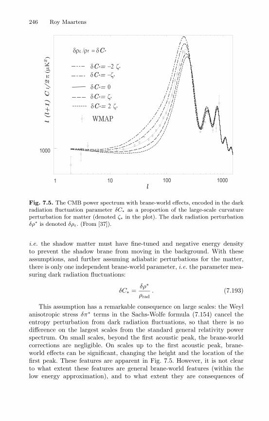
246 Roy Maartens
l (l+
1) C
l/2
π (
µΚ
)
l
δC*= −2 ζ∗
δC*= −ζ∗
δC*= ζ∗
δC*= 2 ζ∗
δC*= 0
WMAP
δρε /ρr = δC*
1
1000
10 100 1000
2
Fig. 7.5. The CMB power spectrum with brane-world effects, encoded in the darkradiation fluctuation parameter δC∗ as a proportion of the large-scale curvatureperturbation for matter (denoted ζ∗ in the plot). The dark radiation perturbationδρ∗ is denoted δρε. (From [37]).
i.e. the shadow matter must have fine-tuned and negative energy densityto prevent the shadow brane from moving in the background. With theseassumptions, and further assuming adiabatic perturbations for the matter,there is only one independent brane-world parameter, i.e. the parameter mea-suring dark radiation fluctuations:
δC∗ =δρ∗
ρrad. (7.193)
This assumption has a remarkable consequence on large scales: the Weylanisotropic stress δπ∗ terms in the Sachs-Wolfe formula (7.154) cancel theentropy perturbation from dark radiation fluctuations, so that there is nodifference on the largest scales from the standard general relativity powerspectrum. On small scales, beyond the first acoustic peak, the brane-worldcorrections are negligible. On scales up to the first acoustic peak, brane-world effects can be significant, changing the height and the location of thefirst peak. These features are apparent in Fig. 7.5. However, it is not clearto what extent these features are general brane-world features (within thelow energy approximation), and to what extent they are consequences of
7 Brane-World Cosmology 247
the simple assumptions imposed on the background. Further work remainsto be done. (A related low energy approximation, using the moduli spaceapproximation, has been developed for certain two-brane models with bulkscalar field [38].)
7.9 Conclusions
Simple brane-world models of RS type provide a rich phenomenology forexploring some of the ideas that are emerging from M theory. These modelsare the simplest brane-worlds with curved extra dimension that allow for ameaningful approach to cosmology. There are generalizations that attemptto make these models more realistic, or that explore other aspects of higher-dimensional gravity which are not probed by these simple models. Importantexamples are:
– The inclusion of dynamical interaction between the brane(s) and a bulkscalar field, described by the action [19, 23]
S =∫d5x√
−(5)g
[ (5)R
2κ25
− 12∂AΦ∂
AΦ− Λ5(Φ)]
+∫
brane(s)d4x
√−g[−λ(Φ) +
K
κ25
+ Lmatter
]. (7.194)
In two-brane models, the brane separation is described by the radion. Forgeneral potentials of the scalar field which provide radion stabilization,4D Einstein gravity is recovered at low energies on either brane. (Bycontrast, in the absence of a bulk scalar, low energy gravity is Brans-Dicke type [13].)In particular, such models will allow some fundamental problems to beaddressed: the hierarchy problem of particle physics; an extra-dimensionalmechanism for initiating inflation (or the hot radiation era with super-Hubble correlations) via brane interaction (building on the initial workin [24, 25]); an extra-dimensional explanation for the dark energy (andpossibly also dark matter) puzzles: could dark energy or late time accel-eration of the universe be a result of gravitational effects on the visiblebrane of the shadow brane, mediated by the bulk dilaton?
– Moduli fields that encode the influence on the brane of further extradimensions (for example, the six extra dimensions in Horava-Witten typesolutions, in addition to the large extra dimension) [38, 47].
– Higher-order curvature invariants, which arise in the AdS/CFT corre-spondence as next-to-leading order corrections in the CFT. These maybe thought of as stringy corrections to the Eisntein-Hilbert action. TheGauss-Bonnet combination in particular has unique properties in 5D, giv-ing field equations which are second-order in the bulk metric (and linearin the second derivatives), and being ghost-free. The action is

248 Roy Maartens
S =∫d5x√
−(5)g
[ (5)R
2κ25
− Λ5
+ α
(5)R2 − 4(5)RAB(5)RAB + (5)RABCD
(5)RABCD]
+∫
braned4x
√−g[−λ+
K
κ25
+ Lmatter
], (7.195)
where α is the Gauss-Bonnet coupling constant, related to the string scale.The cosmological dynamics of these brane-worlds is investigated in [48].In the early universe, the Gauss-Bonnet corrections to the Friedmannequation have the dominant form
H2 ∝ ρ2/3 , (7.196)
so that the high energy behaviour H2 ∝ ρ2 of the RS brane-world isradically modified (although the big bang singularity is not removed).Quantum field theory corrections to the action, arising from the couplingbetween brane matter and bulk gravitons, and leading to an induced4D Ricci term in the brane action. The original induced-gravity brane-world [49] was put forward as an alternative to the RS mechanism: thebulk was flat Minkowski 5D spacetime (and as a consequence there isno normalizable zero-mode of the bulk graviton), and there was no branetension. Another viewpoint is to see the induced-gravity term in the actionas a correction to the RS action:
S =∫d5x√
−(5)g
[ (5)R
2κ25
− Λ5
]
+∫
braned4x
√−g[R
2κ2 − λ+K
κ25
+ Lmatter
]. (7.197)
Unlike the other brane-worlds discussed, these models lead to 5D be-haviour on large scales rather than small scales. The cosmological modelshave been analysed in [50]. The late-universe 5D behaviour of gravitycan naturally produce a late-time acceleration, even without dark energy,although the fine-tuning problem is not evaded.The effect of the induced-gravity correction at early times is to remove thehigh energy ρ2 term in the early universe Friedmann equation; instead,the Friedmann equation is close the standard general relativity form.Thus we have a striking result that both forms of correction to thegravitational action, i.e. Gauss-Bonnet and induced gravity, suppress theRandall-Sundrum type high energy modifications to the Friedmann equa-tion. (Cosmologies with both induced-gravity and Gauss-Bonnet correc-tions to the RS action are considered in [51].)
Brane-world gravity opens up exciting prospects for subjecting M theoryideas to the increasingly stringent tests provided by high-precision astronom-ical observations. In addition, brane-world models provide a rich arena for
7 Brane-World Cosmology 249
probing the geometry and dynamics of the gravitational field and its interac-tion with matter.
Acknowledgments
I thank the organisers for a very enjoyable and stimulating summer school. Iam supported by PPARC.
References
1. For recent reviews, see, e.g., J.H. Schwarz, astro-ph/0304507; J. Polchinski,hep-th/0209105; R. Kallosh, hep-th/0205315.
2. M. Cavaglia, Int. J. Mod. Phys. A18, 1843 (2003), hep-ph/0210296.3. J. Hewett, M. Spiropulu, Ann. Rev. Nucl. Part. Sci. 52, 397 (2002), hep-
ph/0205106.4. P. Horava, E. Witten, Nucl. Phys. B460, 506 (1996), hep-th/9510209.5. A. Lukas, B.A. Ovrut, K.S. Stelle, D. Waldram, Phys. Rev. D59, 086001 (1999),
hep-th/9803235; A. Lukas, B.A. Ovrut, D. Waldram, Phys. Rev. D60, 086001(1999), hep-th/9806022; ibid., 61, 023506 (2000), hep-th/9902071.
6. L. Randall, R. Sundrum, Phys. Rev. Lett. 83, 3370 (1999), hep-ph/9905221.7. L. Randall, R. Sundrum, Phys. Rev. Lett. 83, 4690 (1999), hep-th/9906064.8. N. Arkani-Hamed, S. Dimopoulos, G. Dvali, Phys. Lett. B429, 263 (1998), hep-
ph/9803315; I. Antoniadis, N. Arkani-Hamed, S. Dimopoulos, G. Dvali, Phys.Lett. B436, 257 (1998), hep-ph/9804398.
9. R. Maartens, gr-qc/0312059.10. P. Brax, C. van de Bruck, Class. Quantum Grav. 20, R201 (2003), hep-
th/0303095; N. Deruelle, Astrophys. Space Sci. 283, 619 (2003), gr-qc/0301035;S. Rasanen, astro-ph/0208282; D. Langlois, Prog. Theor. Phys. Suppl. 148,181 (2002), hep-th/0209261; E. Papantonopoulos, Lect. Notes Phys. 592, 458(2002), hep-th/0202044; D. Langlois, gr-qc/0207047; D. Wands, Class. Quan-tum Grav. 19, 3403 (2002), hep-th/0203107; D. Langlois, Int. J. Mod. Phys.A17, 2701 (2002), gr-qc/0205004; J. March-Russell, hep-ph/0012151.
11. D. Langlois, astro-ph/0301021.12. W.D. Goldberger, M.B. Wise, Phys. Rev. Lett. 83, 4922 (1999), hep-
ph/9907447.13. J. Garriga, T. Tanaka, Phys. Rev. Lett. 84, 2778 (2000), hep-th/9911055.14. P. Binetruy, C. Deffayet, U. Ellwanger, D. Langlois, Phys. Lett. B477, 285
(2000), hep-th/9910219.15. P. Kraus, JHEP 12, 011 (1999), hep-th/9910149; N. Kaloper, Phys. Rev. D60,
123506 (1999), hep-th/9905210; A. Kehagias, E. Kiritsis, JHEP 11, 022 (1999),hep-th/9910174; S.S. Gubser, Phys. Rev. D63 084017 (2001), hep-th/9912001;S. Mukohyama, Phys. Lett. B473, 241 (2000), hep-th/9911165; D. Ida, JHEP09, 014 (2000), gr-qc/9912002; E.E. Flanagan, S.-H. Henry Tye, I. Wasserman,Phys. Rev. D 62, 044039 (2000), hep-ph/9910498.
16. J. Garriga, M. Sasaki, Phys. Rev. D62, 043523 (2000), hep-th/9912118.

250 Roy Maartens
17. T. Shiromizu, K. Maeda, M. Sasaki, Phys. Rev. D62, 024012 (2000), gr-qc/9910076.
18. S. Mukohyama, T. Shiromizu, K. Maeda, Phys. Rev. D62, 024028 (2000), hep-th/9912287; P. Bowcock, C. Charmousis, R. Gregory, Class. Quantum Grav.17, 4745 (2000), hep-th/0007177.
19. K. Maeda, D. Wands, Phys. Rev. D62, 124009 (2000), hep-th/0008188.20. R. Maartens, Phys. Rev. D62, 084023 (2000), hep-th/0004166.21. D. Langlois, R. Maartens, M. Sasaki, D. Wands, Phys. Rev. D63, 084009 (2001),
hep-th/0012044.22. J.D. Barrow, R. Maartens, Phys. Lett. B532, 153 (2002), gr-qc/0108073; K.
Ichiki, M. Yahiro, T. Kajino, M. Orito, G.J. Mathews, Phys. Rev. D66, 043521(2002), astro-ph/0203272; J.D. Bratt, A.C. Gault, R.J. Scherrer, T.P. Walker,Phys. Lett. B546, 19 (2002), astro-ph/0208133.
23. S. Kobayashi, K. Koyama, J. Soda, Phys. Lett. B501, 157 (2001), hep-th/0009160; Y. Himemoto, M. Sasaki, Phys. Rev. D63, 044015 (2001), gr-qc/0010035; E.E. Flanagan, S.-H. Henry Tye, I. Wasserman, Phys. Lett. B522,155 (2001), hep-th/0110070; N. Sago, Y. Himemoto, M. Sasaki, Phys. Rev.D65, 024014 (2002), gr-qc/0104033; Y. Himemoto, T. Tanaka, M. Sasaki, Phys.Rev. D65, 104020 (2002), gr-qc/0112027; Y. Himemoto, T. Tanaka, Phys. Rev.D67, 084014 (2003), gr-qc/0212114; T. Tanaka, Y. Himemoto, Phys. Rev. D67,104007 (2003), gr-qc/0301010; B. Wang, L-H. Xue, X. Zhang, W-Y.P. Hwang,Phys. Rev. D67, 123519 (2003), hep-th/0301072; K. Koyama, K. Takahashi,Phys. Rev. D67, 103503 (2003), hep-th/0301165; D. Langlois, M. Sasaki, Phys.Rev. D68, 064012 (2003), hep-th/0302069; Y. Himemoto, M. Sasaki, Prog.Theor. Phys. Suppl. 148, 235 (2002), gr-qc/0302054; R.H. Brandenberger, G.Geshnizjani, S. Watson, Phys. Rev. D67, 123510 (2003), hep-th/0302222; M.Minamitsuji, Y. Himemoto, M. Sasaki, Phys. Rev. D68, 024016 (2003), gr-qc/0303108; S. Kanno, J. Soda, hep-th/0303203; J. Martin, G.N. Felder, A.V.Frolov, M. Peloso, L. Kofman, hep-th/0309001; A.V. Frolov, L. Kofman, hep-th/0309002; P.R. Ashcroft, C. van de Bruck, A.-C. Davis, astro-ph/0310643.
24. G. Dvali, S.-H.H. Tye, Phys. Lett. B450, 72 (1999), hep-ph/9812483; S. Kanno,M. Sasaki, J. Soda, Prog. Theor. Phys. 109, 357 (2003), hep-th/0210250.
25. J. Khoury, B.A. Ovrut, P.J. Steinhardt, N. Turok, Phys. Rev. D64, 123522(2001), hep-th/0103239; R. Kallosh, L. Kofman, A. Linde, Phys. Rev. D64,123523 (2001), hep-th/0104073; A. Neronov, JHEP 11, 007 (2001), hep-th/0109090; P.J. Steinhardt, N. Turok, Phys. Rev. D65, 126003 (2002), hep-th/0111098; D. Langlois, K. Maeda, D. Wands, Phys. Rev. Lett. 88, 181301(2002), gr-qc/0111013; N.E. Mavromatos, hep-th/0210008; A.J. Tolley, N.Turok, P.J. Steinhardt, hep-th/0306109.
26. R. Maartens, D. Wands, B.A. Bassett, I.P.C. Heard, Phys. Rev. D62, 041301(2000), astro-ph/0009131.
27. N. Kaloper, Phys. Rev. D60, 123506 (1999), hep-th/9905210; J.M. Cline, C.Grojean, G. Servant, Phys. Rev. Lett. 83, 4245 (1999), hep-ph/9906523; H.Stoica, S.-H. Henry Tye, I. Wasserman, Phys. Lett. B482, 205 (2000), hep-th/0004126; L. Mendes, A.R. Liddle, Phys. Rev. D62, 103511 (2000), astro-ph/0006020; A. Mazumdar, Phys. Rev. D64, 027304 (2001), hep-ph/0007269;S.C. Davis, W.B. Perkins, A.-C. Davis, I.R. Vernon, Phys. Rev. D63, 083518(2001), hep-ph/0012223; A.R. Liddle, A.N. Taylor, Phys. Rev. D65, 041301(2002), astro-ph/0109412; M.C. Bento, O. Bertolami, Phys. Rev. D65, 063513

7 Brane-World Cosmology 251
(2002), astro-ph/0111273; M.C. Bento, O. Bertolami, A.A. Sen, Phys. Rev.D67, 023504 (2003), gr-qc/0204046; ibid., 063511 (2003), hep-th/0208124;S. Mizuno, K. Maeda, K. Yamamoto, Phys. Rev. D67, 024033 (2003), hep-ph/0205292; R. Hawkins, J.E. Lidsey, Phys. Rev. D68, 083505 (2003), astro-ph/0306311; K.E. Kunze, hep-th/0310200.
28. E.J. Copeland, A.R. Liddle, J.E. Lidsey, Phys. Rev. D64, 023509 (2001),astro-ph/0006421; A. S. Majumdar, Phys. Rev. D64, 083503 (2001), astro-ph/0105518; V. Sahni, M. Sami, T. Souradeep, Phys. Rev. D65, 023518 (2002),gr-qc/0105121; N.J. Nunes, E.J. Copeland, Phys. Rev. D66, 043524 (2002),astro-ph/0204115; A.R. Liddle, L.A. Urena-Lopez, Phys. Rev. D68, 043517(2003), astro-ph/0302054.
29. G. Huey, J.E. Lidsey, Phys. Lett. B514, 217 (2001), astro-ph/0104006.30. A. Albrecht, C.P. Burgess, F. Ravndal, C. Skordis, Phys. Rev. D65, 123507
(2002), astro-ph/0107573; S. Mizuno, K. Maeda, Phys. Rev. D64, 123521(2001), hep-ph/0108012; J.E. Lidsey, T. Matos, L.A. Urena-Lopez, Phys. Rev.D66, 023514 (2002), astro-ph/0111292; C.P. Burgess, astro-ph/0207174; D.Seery, B.A. Bassett, astro-ph/0310208.
31. D. Wands, K. A. Malik, D. H. Lyth, A. R. Liddle, Phys. Rev. D62, 043527(2000), astro-ph/0003278.
32. A.R. Liddle, A.J. Smith, Phys. Rev. D68, 061301 (2003), astro-ph/0307017.33. D. Langlois, R. Maartens, D. Wands, Phys. Lett. B489, 259 (2000), hep-
th/0006007.34. D.S. Gorbunov, V.A. Rubakov, S.M. Sibiryakov, JHEP 10, 15 (2001), hep-
th/0108017.35. H.A. Bridgman, K.A. Malik, D. Wands, Phys. Rev. D63, 084012 (2001), hep-
th/0010133.36. J. Soda, S. Kanno, Phys. Rev. D66, 083506 (2002), hep-th/0207029; T. Wise-
man, Class. Quantum Grav. 19, 3083 (2002), hep-th/0201127; T. Shiromizu, K.Koyama, Phys. Rev. D67, 084022 (2003), hep-th/0210066; J. Soda, S. Kanno,Astrophys. Space Sci. 283, 639 (2003), gr-qc/0209086; ibid., hep-th/0303203.
37. K. Koyama, Phys. Rev. Lett., in press (2003), astro-ph/0303108.38. C.S. Rhodes, C. van de Bruck, Ph. Brax, A.C. Davis, Phys. Rev. D68, 083511
(2003), astro-ph/0306343; P. Brax, C. van de Bruck, A.-C. Davis, C.S. Rhodes,hep-ph/0309181.
39. T. Hiramatsu, K. Koyama, A. Taruya, hep-th/0308072.40. R. Easther, D. Langlois, R. Maartens, D. Wands, JCAP 10, 014 (2003), hep-
th/0308078.41. S. Mukohyama, Phys. Rev. D62, 084015 (2000), hep-th/0004067; S. Muko-
hyama, Phys. Rev. D64, 064006 (2001), hep-th/0104185.42. H.A. Bridgman, K.A. Malik, D. Wands, Phys. Rev. D65, 043502 (2002), astro-
ph/0107245.43. K. Koyama, Phys. Rev. D66, 084003 (2002), gr-qc/0204047.44. A. Frolov, L. Kofman, hep-th/0209133.45. T. Kobayashi, H. Kudoh, T. Tanaka, Phys. Rev. D68, 044025 (2003), gr-
qc/0305006.46. K. Koyama, unpublished notes.47. R. Brustein, S.P. de Alwis, E.G. Novak, Phys. Rev. D68, 043507 (2003), hep-
th/0212344; L. Kofman, astro-ph/0303614; S. Kachru, R. Kallosh, A. Linde, J.Maldacena, L. McAllister, S.P. Trivedi, JCAP 10, 013 (2003), hep-th/0308055;M. Peloso, E. Poppitz, hep-ph/0307379; J. Gray, A. Lukas, hep-th/0309096.
252 Roy Maartens
48. N. Deruelle, T. Dolezel, Phys. Rev. D62, 103502 (2000), gr-qc/0004021; C.Germani, C.F. Sopuerta, Phys. Rev. Lett. 88, 231101 (2002), hep-th/0202060;C. Charmousis, J-F. Dufaux, Class. Quantum Grav. 19, 4671 (2002), hep-th/0202107; P. Binetruy, C. Charmousis, S.C. Davis, J.-F. Dufaux, Phys. Lett.B544, 183 (2002), hep-th/0206089; N.E. Mavromatos, J. Rizos, Int. J. Mod.Phys. A18, 57 (2003), hep-th/0205299; J.E. Lidsey, N.J. Nunes, Phys. Rev.D67, 103510 (2003), astro-ph/0303168; N. Deruelle, J. Madore, gr-qc/0305004;C. Barcelo, C. Germani, C.F. Sopuerta, Phys. Rev. D68, 104007 (2003), gr-qc/0306072; N. Deruelle, C. Germani, gr-qc/0306116; C. Charmousis, S.C.Davis, J.-F. Dufaux, hep-th/0309083; K. Maeda, T. Torii, hep-th/0309152.
49. G. Dvali, G. Gabadadze, M. Porrati, Phys. Lett. B485, 208 (2000), hep-th/0005016. See also, H. Collins, B. Holdom, Phys. Rev. D62, 105009 (2000),hep-ph/0003173; Yu.V. Shtanov, hep-th/0005193.
50. C. Deffayet, G. Dvali, G. Gabadadze, Phys. Rev. D65, 044023 (2002), astro-ph/0105068; G. Kofinas, JHEP 08, 034 (2001), hep-th/0108013; G.A. Diaman-dis, B.C. Georgalas, N.E. Mavromatos, E. Papantonopoulos, I. Pappa, Int. J.Mod. Phys. A17, 2241 (2002), hep-th/0107124; E. Kiritsis, N. Tetradis, T.N.Tomaras, JHEP 03, 019 (2002), hep-th/0202037; C. Deffayet, S.J. Landau,J. Raux, M. Zaldarriaga, P. Astier, Phys. Rev. D66, 024019 (2002), astro-ph/0201164; V. Sahni, Y. Shtanov, astro-ph/0202346; Y. Shtanov, V. Sahni,Class. Quantum Grav. 19, L101 (2002), gr-qc/0204040; V. Sahni, Y. Shtanov,Int. J. Mod. Phys. D11, 1 (2002), gr-qc/0205111; P. Singh, R.G. Vishwakarma,N.K. Dadhich, hep-th/0206193; U. Alam, V. Sahni, astro-ph/0209443; K.Maeda, S. Mizuno, T. Torii, Phys. Rev. D68, 024033 (2003), gr-qc/0303039;A. Lue, G. Starkman, Phys. Rev. D67, 064002 (2003), astro-ph/0212083; T.Multamaki, E. Gaztanaga, M. Manera, Mon. Not. Roy. Astron. Soc. 344, 761(2003), astro-ph/0303526; B. Gumjudpai, gr-qc/0308046.
51. G. Kofinas, R. Maartens, E. Papantonopoulos, JHEP 10, 066 (2003), hep-th/0307138.
8 Gravitational Wave Astronomy:The High Frequency Window
Nils Andersson1 and Kostas D. Kokkotas2,3
1 School of Mathematics, University of Southampton, Southampton SO17 1BJ,UK
2 Department of Physics, Aristotle University of Thessaloniki, Thessaloniki541 24 Greece
3 Center for Gravitational Wave Physics, 104 Davey Laboratory, University Park,PA 16802, USA
Abstract. As several large scale interferometers are beginning to take data at sen-sitivities where astrophysical sources are predicted, the direct detection of gravita-tional waves may well be imminent. This would (finally) open the long anticipatedgravitational-wave window to our Universe, and should lead to a much improvedunderstanding of the most violent processes imaginable; the formation of black holesand neutron stars following core collapse supernovae and the merger of compactobjects at the end of binary inspiral. Over the next decade we can hope to learnmuch about the extreme physics associated with, in particular, neutron stars.
This contribution is divided in two parts. The first part provides a text-booklevel introduction to gravitational radiation. The key concepts required for a dis-cussion of gravitational-wave physics are introduced. In particular, the quadrupoleformula is applied to the anticipated “bread-and-butter” source for detectors likeLIGO, GEO600, EGO and TAMA300: inspiralling compact binaries. The secondpart provides a brief review of high frequency gravitational waves. In the frequencyrange above (say) 100 Hz, gravitational collapse, rotational instabilities and oscil-lations of the remnant compact objects are potentially important sources of grav-itational waves. Significant and unique information concerning the various stagesof collapse, the evolution of protoneutron stars and the details of the supranu-clear equation of state of such objects can be drawn from careful study of thegravitational-wave signal. As the amount of exciting physics one may be able tostudy via the detections of gravitational waves from these sources is truly inspir-ing, there is strong motivation for the development of future generations of groundbased detectors sensitive in the range from hundreds of Hz to several kHz.
8.1 Introduction
One of the central predictions of Einsteins’ general theory of relativity isthat gravitational waves will be generated as masses are accelerated. De-spite decades of effort these ripples in spacetime have still not been ob-served directly. Yet we have strong indirect evidence for their existence fromthe excellent agreement between the observed inspiral rate of the binarypulsar PSR1913+16 and the theoretical prediction (better than 1% in thephase evolution). This provides confidence in the theory and suggests that
N. Andersson and K.D. Kokkotas, Gravitational Wave Astronomy: The High Frequency Window,Lect. Notes Phys. 653, 255–276 (2005)http://www.springerlink.com/ c© Springer-Verlag Berlin Heidelberg 2005

256 Nils Andersson and Kostas D. Kokkotas
“gravitational-wave astronomy” should be viewed as a serious proposition.Provided that i) detectors with the required sensitivity can be constructed,and ii) the significant data analysis challenge can be dealt with, this new win-dow to the Universe promises to bring unprecedented insights into the mostviolent events imaginable; supernova explosions, binary mergers and the bigbang itself. A key reason for this expectation follows from a comparison be-tween gravitational and electromagnetic waves:
– While electromagnetic waves are radiated by individual particles, gravi-tational waves are due to non-spherical bulk motion of matter. In essence,this means that the information carried by electromagnetic waves isstochastic in nature, while the gravitational waves provide insights intocoherent mass currents.
– The electromagnetic waves will have been scattered many times. In con-trast, gravitational waves interact weakly with matter and arrive at theEarth in pristine condition. This means that gravitational waves can beused to probe regions of space that are opaque to electromagnetic waves,It is, of course, a blessing in disguise since the weak interaction withmatter also makes the gravitational waves fiendishly hard to detect.
– Standard astronomy is based on deep imaging of small fields of view, whilegravitational-wave detectors cover virtually the entire sky.
– Electromagnetic radiation has a wavelength smaller than the size of theemitter, while the wavelength of a gravitational wave is usually largerthan the size of the source. This means that we cannot use gravitational-wave data to create an image of the source. In fact, gravitational-waveobservations are more like audio than visual.
Morale: Gravitational waves carry information which would be very difficultto glean by other means. By analysing gravitational-wave data we can expectto learn a lot about the extreme physics governing compact objects. Thisshould lead to answers to many outstanding questions in astrophysics, forexample,
– What is the black-hole population of the Universe? Observations of thenonlinear spacetime dynamics associated with binary merger, as well asthe quasinormal mode (QNM) ringing which is likely to dominate theradiation at late times, should provide direct proof of the presence of ablack hole, as well as a measure of it’s mass and spin.
– Are astrophysical black holes, indeed, described by the Kerr metric? Bystudying the inspiral of a low-mass object into a supramassive black hole(as anticipated at the center of most galaxies) we can hope to constructa detailed map of the exterior black-hole spacetime.
– What is the supranuclear neutron star equation of state? This is avery difficult question, which potentially involves an understanding ofthe role of exotic phases of matter, like deconfined quarks, superfluid-ity/conductivity, extreme magnetic fields etcetera. At an immediate level,
8 Gravitational Wave Astronomy: The High Frequency Window 257
gravitational-wave observations of the various oscillation modes of a com-pact star may be used to solve the “inverse problem” for parameters likethe mass and the radius of the star. At a more subtle level, the spectrum ofthe star depends on the internal physics. For example, strong compositiongradients which affect the gravity g-modes significantly, and superfluiditywhich leads to the existence of new classes of oscillations associated withthe more or less decoupled additional degrees of freedom of such a system.Finally, the internal physics also plays a crucial role in determining theextent to which various rotational instabilities will be able to grow to aninteresting amplitude. In the case of the Coriolis driven r-modes, theirinstability may be severely suppressed by the presence of hyperons in thestars core. A key role is also played by the internal magnetic fields.
At the time of writing, the new generation of interferometric gravitational-wave detectors (in particular LIGO and GEO600) is already collecting data ata sensitivity at least one order of magnitude better than that of the operatingresonant detectors. In the first instance, the broadband detectors will besensitive in a range of frequencies between 50 and a few hundred Hz. Thisfrequency window is of great interest since an inspiraling compact binary willmove through it during the last few minutes before merger. Such sources arethe natural “bread and butter” source for the detectors. The next generationof interferometers will broaden the bandwidth somewhat but will still not bevery sensitive to frequencies above 500-600 Hz, unless they are operated ina narrow-band configuration [1, 2]. There are also interesting suggestions forwide band resonant detectors in the kHz band [3]. The move towards higherfrequencies is driven by the wealth of exciting sources that radiate in therange from a few hundred Hz up to several kHz.
Our contribution to these proceedings is divided in two parts. The firstpart describes gravitational-wave physics at an introductory level. The secondpart provides a brief review of the main sources that radiate in the frequencyband above a few hundred Hz. We believe that these sources are the naturaltargets for a third generation of ground based detectors. As we will discuss,there are a variety of sources associated with very interesting physics in thishigh-frequency window. These sources clearly deserve special attention, andif either resonant or narrow-band interferometers can achieve the requiredsensitivity, a plethora of unique information can be gathered.
8.2 Einstein’s Elusive Waves
The aim of the first part of our contribution is to provide a condensed text-book level introduction to gravitational waves. Although in no sense completethis description should prepare the reader for the discussion of high-frequencysources which follows.
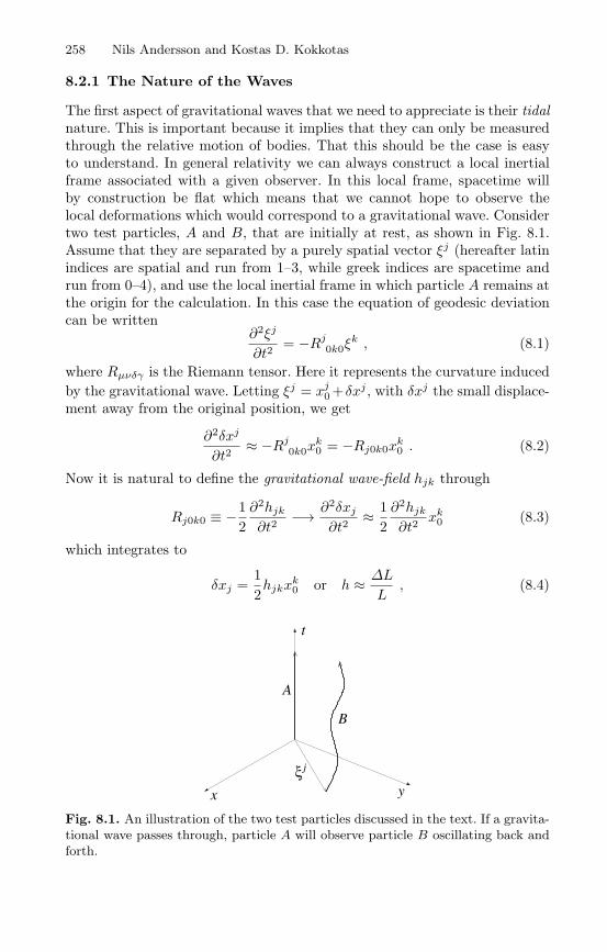
258 Nils Andersson and Kostas D. Kokkotas
8.2.1 The Nature of the Waves
The first aspect of gravitational waves that we need to appreciate is their tidalnature. This is important because it implies that they can only be measuredthrough the relative motion of bodies. That this should be the case is easyto understand. In general relativity we can always construct a local inertialframe associated with a given observer. In this local frame, spacetime willby construction be flat which means that we cannot hope to observe thelocal deformations which would correspond to a gravitational wave. Considertwo test particles, A and B, that are initially at rest, as shown in Fig. 8.1.Assume that they are separated by a purely spatial vector ξj (hereafter latinindices are spatial and run from 1–3, while greek indices are spacetime andrun from 0–4), and use the local inertial frame in which particle A remains atthe origin for the calculation. In this case the equation of geodesic deviationcan be written
∂2ξj
∂t2= −Rj
0k0ξk , (8.1)
where Rµνδγ is the Riemann tensor. Here it represents the curvature inducedby the gravitational wave. Letting ξj = xj
0 +δxj , with δxj the small displace-ment away from the original position, we get
∂2δxj
∂t2≈ −Rj
0k0xk0 = −Rj0k0x
k0 . (8.2)
Now it is natural to define the gravitational wave-field hjk through
Rj0k0 ≡ −12∂2hjk
∂t2−→ ∂2δxj
∂t2≈ 1
2∂2hjk
∂t2xk
0 (8.3)
which integrates to
δxj =12hjkx
k0 or h ≈ ∆L
L, (8.4)
x y
t
jξ
A
B
Fig. 8.1. An illustration of the two test particles discussed in the text. If a gravita-tional wave passes through, particle A will observe particle B oscillating back andforth.
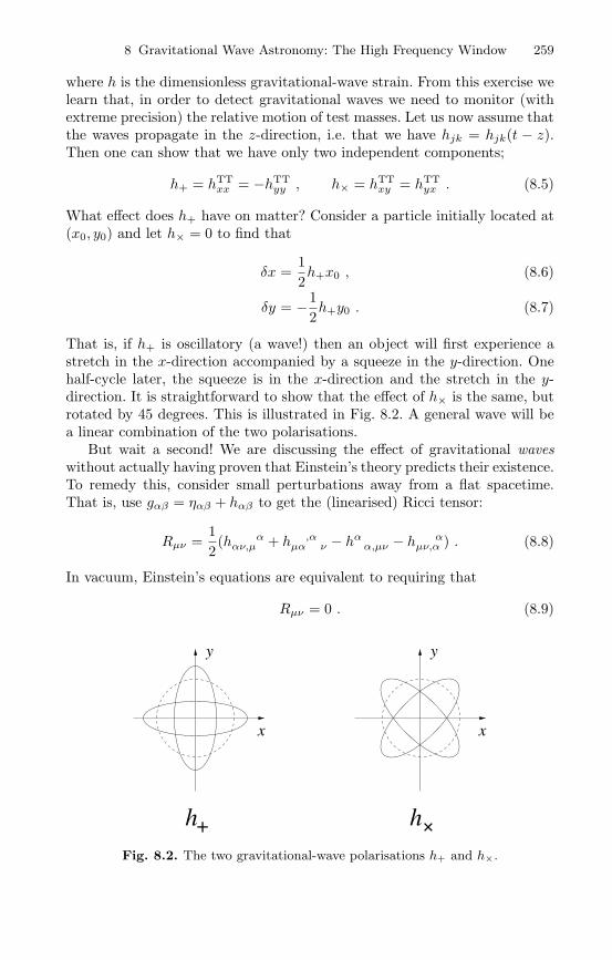
8 Gravitational Wave Astronomy: The High Frequency Window 259
where h is the dimensionless gravitational-wave strain. From this exercise welearn that, in order to detect gravitational waves we need to monitor (withextreme precision) the relative motion of test masses. Let us now assume thatthe waves propagate in the z-direction, i.e. that we have hjk = hjk(t − z).Then one can show that we have only two independent components;
h+ = hTTxx = −hTT
yy , h× = hTTxy = hTT
yx . (8.5)
What effect does h+ have on matter? Consider a particle initially located at(x0, y0) and let h× = 0 to find that
δx =12h+x0 , (8.6)
δy = −12h+y0 . (8.7)
That is, if h+ is oscillatory (a wave!) then an object will first experience astretch in the x-direction accompanied by a squeeze in the y-direction. Onehalf-cycle later, the squeeze is in the x-direction and the stretch in the y-direction. It is straightforward to show that the effect of h× is the same, butrotated by 45 degrees. This is illustrated in Fig. 8.2. A general wave will bea linear combination of the two polarisations.
But wait a second! We are discussing the effect of gravitational waveswithout actually having proven that Einstein’s theory predicts their existence.To remedy this, consider small perturbations away from a flat spacetime.That is, use gαβ = ηαβ + hαβ to get the (linearised) Ricci tensor:
Rµν =12(h α
αν,µ + h ,αµα ν − hα
α,µν − h αµν,α ) . (8.8)
In vacuum, Einstein’s equations are equivalent to requiring that
Rµν = 0 . (8.9)
y
x
y
x
h h+ +Fig. 8.2. The two gravitational-wave polarisations h+ and h×.

260 Nils Andersson and Kostas D. Kokkotas
Now consider what happens if we make a coordinate transformation. For
xα → xα + ξα (8.10)
we gethµν → hµν − ξµ,ν − ξν,µ . (8.11)
Use this freedom to impose the harmonic gauge condition h ,αµα = 0. Since
the gauge remains unchanged for any transformation such that ξµ = 0, wecan impose further conditions. We take one of these to be h α
α = 0, to get
h αµν,α = hµν = 0 . (8.12)
That is, the metric variations are governed by a standard wave equation.Finally, use h00 = hj0 = h0j = 0 to get hjk = hTT
jk as before. The set ofcoordinates we have introduced is known as TT-gauge.
Before we move on to discuss the modelling of various gravitational-wavesources, it is worth elucidating an issue that caused serious debate until thelate 1960s. We need to demonstrate that gravitational waves carry energy.This is a tricky problem because, as we have already pointed out, one canonly deduce the presence of a wave from the relative effect on two (or more)test particles. This means that one cannot localize the wave to individualpoints in space, and hence cannot directly “measure” its energy. In orderto construct a meaningful energy expression we need to average over one(or more) wavelengths. Defining perturbations with respect to an averagedspacetime metric, i.e. using
g(B)µν = 〈gµν〉 −→ gµν = g(B)
µν + hµν . (8.13)
and expanding in powers of h (which is presumed small), we have the(schematic) Einstein equations,
〈Gµν〉 = GBµν +
⟨G(1)
µν
⟩
︸ ︷︷ ︸O(hµν)
+⟨G(2)
µν
⟩
︸ ︷︷ ︸O(h..h..)
= 0 . (8.14)
Here, the term that is linear in h will vanish if we average over a wavelength.This means that we can deduce an expression for the stress energy-tensor forgravitational waves:
GBµν = −8π
⟨G
(2)µν
8π
⟩
≡ 8πTGWµν . (8.15)
Working out the algebra one can show that, in TT-gauge we will have
TGWµν =
132π
⟨hTT
ij,µhTTij
,ν
⟩. (8.16)
In particular, the energy propagating in the z-direction then follows from
8 Gravitational Wave Astronomy: The High Frequency Window 261
TGW0z = −TGW
00 = − 116π
⟨h2
+ + h2×⟩
−→ E = −TGW0z =
ω2
16π⟨h2
+ + h2×⟩.
(8.17)where the frequency of the wave is ω. Finally assuming that h+ ∼ h× ∼h sinω(t− z), and integrating over a sphere with radius r, we get
E =ω2r2
4h2 → |h|2 =
4Gc3r2
E . (8.18)
As we will now demonstrate, this is a very useful relation.
8.2.2 Estimating the Gravitational-Wave Amplitude
We can use the expression (8.18) to infer the gravitational-wave strain as-sociated with typical gravitational-wave sources. Let us characterise a givenevent by a timescale τ and assume that the signal is monochromatic (withfrequency f). Then we can use dE/dt ≈ E/τ and h ≈ 2πfh to deduce that
h ≈ 5 × 10⁻²²(
E
10−3Mc2
)1/2 ( τ
1 ms
)−1/2(
f
1 kHz
)−1(r
15 Mpc
)−1
.
(8.19)If the signal analysis is based on matched filtering, the effective amplitudeimproves roughly as the square root of the number of observed cycles n.Using n ≈ fτ we get
hc ≈ 5 × 10⁻²²(
E
10−3Mc2
)1/2(f
1 kHz
)−1/2(r
15 Mpc
)−1
. (8.20)
This is a crucial expression. We see that the “detector sensitivity” essentiallydepends only on the radiated energy, the characteristic frequency and thedistance to the source. That is, in order to obtain a rough estimate of therelevance of a given gravitational-wave source at a given distance we onlyneed to estimate the frequency and the radiated energy. Alternatively, if weknow the energy released can work out the distance at which these sourcescan be detected.
It is quite easy to obtain a rough idea of the frequencies involved. Thedynamical frequency of any self-bound system with mass M and radius R is
f ≈ 12π
√GM
R3 . (8.21)
Thus, the natural frequency of a (non-rotating) black hole should be
fBH ≈ 104(MM
)Hz . (8.22)
Medium sized black holes, with masses in the range 10 − 100M, will beprime sources for ground-based interferometers, while black holes with masses

262 Nils Andersson and Kostas D. Kokkotas
∼ 106M should radiate in the LISA bandwidth. Meanwhile, neutron stars,with a mass of 1.4M compressed inside a radius of 10 km, will radiate at
fNS ≈ 2 kHz . (8.23)
This means that one would expect neutron physics to be in the range forground based detectors. In fact, given the likely need to detect signals withfrequencies above 1 kHz, neutron star signals provide a strong motivation forthe development of (third generation) high-frequency detectors.
Given that the weak signals are going to be buried in detector noise, weneed to obtain as accurate theoretical models as possible. The rough orderof magnitude estimates we just derived will certainly not be sufficient, eventhough they provide an indication as to whether it is worth spending thetime and effort required to build a detailed model. Such source models aretypically obtained using either
– approximate perturbation techniques, eg. expansions in small perturba-tions away from a known solution to the Einstein equations, the archetypalcase being black-hole and neutron star oscillations.
– post-Newtonian approximations, essentially an expansion in the ratio be-tween a characteristic velocity of the system and the speed of light, mostoften used to model the inspiral phase of a compact binary system.
– numerical relativity, where the Einstein equations are formulated as aninitial-value problem and solved on the computer. This is the only wayto make progress in situations where the full nonlinearities of the theorymust be included, eg. in the merger of black holes and neutron stars or asupernova core collapse.
Here we will only describe the first step beyond a Newtonian description,where the gravitational radiation is described by the so-called quadrupoleformula. For a source with weak internal gravity we have (in TT-gauge)
hµν = −16πTµν . (8.24)
We can solve this equation using the standard retarded Green’s function toget
hµν(t,x) = 4∫Tµν(x′, t′ = t− |x − x′|)
|x − x′| d3x . (8.25)
Matching of the near-zone solution to an outgoing wave solution far awayleads to the expression
hTTjk =
2Grc4
I–TTjk (t− r) , (8.26)
where
I–jk ≡∫ρ
(xjxk − 1
3r2δjk
)d3x . (8.27)
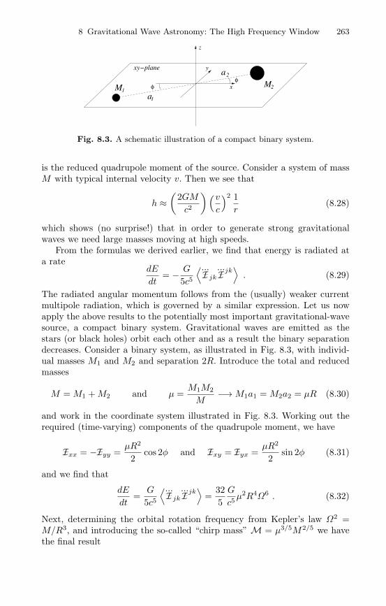
8 Gravitational Wave Astronomy: The High Frequency Window 263
M Ma
xy−plane
1
12
a2
z
y
xφ
φ
Fig. 8.3. A schematic illustration of a compact binary system.
is the reduced quadrupole moment of the source. Consider a system of massM with typical internal velocity v. Then we see that
h ≈(
2GMc2
)(vc
)2 1r
(8.28)
which shows (no surprise!) that in order to generate strong gravitationalwaves we need large masses moving at high speeds.
From the formulas we derived earlier, we find that energy is radiated ata rate
dE
dt= − G
5c5⟨...I– jk
...I– jk⟩. (8.29)
The radiated angular momentum follows from the (usually) weaker currentmultipole radiation, which is governed by a similar expression. Let us nowapply the above results to the potentially most important gravitational-wavesource, a compact binary system. Gravitational waves are emitted as thestars (or black holes) orbit each other and as a result the binary separationdecreases. Consider a binary system, as illustrated in Fig. 8.3, with individ-ual masses M1 and M2 and separation 2R. Introduce the total and reducedmasses
M =M1 +M2 and µ =M1M2
M−→M1a1 =M2a2 = µR (8.30)
and work in the coordinate system illustrated in Fig. 8.3. Working out therequired (time-varying) components of the quadrupole moment, we have
I–xx = −I–yy =µR2
2cos 2φ and I–xy = I–yx =
µR2
2sin 2φ (8.31)
and we find that
dE
dt=G
5c5⟨...I– jk
...I– jk⟩
=325G
c5µ2R4Ω6 . (8.32)
Next, determining the orbital rotation frequency from Kepler’s law Ω2 =M/R3, and introducing the so-called “chirp mass” M = µ3/5M2/5 we havethe final result
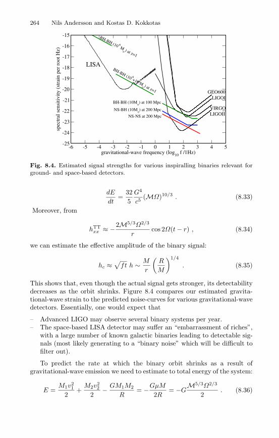
264 Nils Andersson and Kostas D. Kokkotas
-6 -5 -4 -3 -2 -1 0 1 2 3 4 5gravitational-wave frequency (log
10 f /1Hz)
-25
-24
-23
-22
-21
-20
-19
-18
-17
-16
-15
spec
tral
sen
sitiv
ity (
stra
in p
er r
oot H
z)
LISA
GEO600LIGOI
VIRGOLIGOIINS-NS at 200 Mpc
NS-BH (10Mo) at 200 Mpc
BH-BH (10Mo) at 100 Mpc
BH-BH (10 6 M
o ) at z=1
BH-BH (10 6+10 M
o ) at z=1
Fig. 8.4. Estimated signal strengths for various inspiralling binaries relevant forground- and space-based detectors.
dE
dt=
325G4
c5(MΩ)10/3 . (8.33)
Moreover, from
hTTxx ≈ −2M5/3Ω2/3
rcos 2Ω(t− r) , (8.34)
we can estimate the effective amplitude of the binary signal:
hc ≈√ft h ∼ M
r
(R
M
)1/4
. (8.35)
This shows that, even though the actual signal gets stronger, its detectabilitydecreases as the orbit shrinks. Figure 8.4 compares our estimated gravita-tional-wave strain to the predicted noise-curves for various gravitational-wavedetectors. Essentially, one would expect that
– Advanced LIGO may observe several binary systems per year.– The space-based LISA detector may suffer an “embarrassment of riches”,
with a large number of known galactic binaries leading to detectable sig-nals (most likely generating to a “binary noise” which will be difficult tofilter out).
To predict the rate at which the binary orbit shrinks as a result ofgravitational-wave emission we need to estimate to total energy of the system:
E =M1v
21
2+M2v
22
2− GM1M2
R= −GµM
2R= −GM5/3Ω2/3
2. (8.36)
8 Gravitational Wave Astronomy: The High Frequency Window 265
From this we find that the period P of the system changes as
P
P= −96
5G3
c5M5/3Ω8/3 . (8.37)
For the binary pulsar 1913+16, the predicted change in orbital period agreeswith the theoretical prediction to within 1%. This indirect proof that gravi-tational waves exist led to Hulse and Taylor being awarded the 1993 Nobelprize in physics.
Finally, note that that the chirp-mass M plays a key role in our variousexpressions. From
P
P∼ M5/3Ω8/3 and h ∼ M5/3Ω2/3
r, (8.38)
we see that this is the only combination of the two masses that can be inferedfrom the signal (at this level of approximation: higher order post-Newtoniancorrections depend on the individual masses, the spins etcetera). Suppose thatwe detect both the change in the amplitude h and the shift in the frequency.Then one can infer both the chirp mass and the distance to the source, and ineffect coalescing binaries are standard candles which can be used to constraincosmological parameters.
One often classifies gravitational-wave sources by the nature of the waves.This is convenient because the different classes require different approachesto the data-analysis problem;
– Chirps. As a binary system radiates gravitational waves and loses energythe two constituents spiral closer together. As the separation decreases thegravitational-wave amplitude increases, leading to a characteristic “chirp”signal.
– Bursts. Many scenarios lead to burst-like gravitational waves. A typicalexample would be black-hole oscillations excited during binary merger.
– Periodic. Systems where the gravitational-wave backreaction leads toa slow evolution (compared to the observation time) may radiate per-sistent waves with a virtually constant frequency. This would be thegravitational-wave analogue of the radio pulsars.
– Stochastic. A stochastic (non-thermal) background of gravitational wavesis expected to have been generated following the Big Bang. One may alsohave to deal with stochastic gravitational-wave signals when the sourcesare too abundant for us to distinguish them as individuals.
8.3 High-Frequency Gravitational Wave Sources
Having introduced the key concepts required for a discussion of gravitational-wave physics we will now focus our attention on sources that radiate above a

266 Nils Andersson and Kostas D. Kokkotas
hundred Hz or so, i.e. which may at least in principle be detectable from theground. As we will see there are strong motivations for constructing detectorswhich are sensitive up to (ideally) several kHz.
8.3.1 Radiation from Binary Systems
It is easy to understand why binary systems are considered the “best” sourcesof gravitational waves. They emit copious amounts or gravitational radiation,and for a given system we know quite accurately the amplitude and frequencyof the gravitational waves in terms of the masses of the two bodies and theirseparation (see Sect. 8.2.2).
The gravitational-wave signal from inspiraling binaries is approximatelysinusoidal, see equation (8.34), with a frequency which is twice the orbitalfrequency of the binary. As the binary system evolves the orbit shrinks andthe frequency increases in the characteristic chirp. Eventually, dependingon the masses of the binaries, the frequency of the emitted gravitationalwaves will enter the bandwidth of the detector at the low-frequency endand will evolve quite fast towards higher frequencies. A system consistingof two neutron stars will be detectable by LIGO when the frequency of thegravitational waves is ∼10Hz until the final coalescence around 1 kHz. Thisprocess will last for about 15 min and the total number of observed cycles willbe of the order of 104, which leads to an enhancement of the detectabilityby a factor 100 (remember hc ∼ √
nh). Binary neutron star systems andbinary black hole systems with masses of the order of 50M are the primarysources for LIGO. Given the anticipated sensitivity of LIGO, binary blackhole systems are the most promising sources and could be detected as far as200 Mpc away. For the present estimated sensitivity of LIGO the event rateis probably a few per year, but future improvements of detector sensitivity(the LIGO II phase) could lead to the detection of at least one event permonth. Supermassive black hole systems of a few million solar masses arethe primary source for LISA. These binary systems are rare, but due to thehuge amount of energy released, they should be detectable from as far awayas the boundaries of the observable universe. Finally, the recent discovery ofthe highly relativistic binary pulsar J0737-3039 [4] enchanced considerablythe expected coalescence event rate of NS-NS binaries [5]. The event rate forinitial LIGO is in the best case 0.2 per year while advanced LIGO might beable to detect 20-1000 events per year.
8.3.2 Gravitational Collapse
One of the most spectacular events in the Universe is the supernova (SN)collapse to create a neutron star (NS) or a black hole (BH). Core collapse isa very complicated event and a proper study demands a deep understandingof neutrino emission, amplification of the magnetic fields, angular momen-tum distribution, pulsar kicks, etc. There are many viable models for each of

8 Gravitational Wave Astronomy: The High Frequency Window 267
the above issues but it is still not possible to combine all of them togetherinto a consistent explanation. Gravitational waves emanating from the veryfirst moments of the core collapse might shed light on all the above problemsand help us understand the details of this dramatic event. Gravitational col-lapse compresses matter to nuclear densities, and is responsible for the corebounce and the shock generation. The event proceeds extremely fast, lastingless than a second, and the dense fluid undergoes motions with relativisticspeeds (v/c ∼ 0.2 − 0.4). Even small deviations from spherical symmetryduring this phase can generate significant amounts of gravitational waves.However, the size of these asymmetries is not known. From observations inthe electromagnetic spectrum we know that stars more massive than ∼ 8Mend their evolution in core collapse and that ∼ 90% of them are stars withmasses ∼ 8 − 20M. During the collapse most of the material is ejected andif the progenitor star has a mass M 20M it leaves behind a neutron star.If M 20M more than 10% falls back and pushes the proto-neutron-star(PNS) above the maximum NS mass leading to the formation of a black hole(type II collapsars). Finally, if the progenitor star has a mass M 40Mno supernova takes place. Instead, the star collapses directly to a BH (type Icollapsars).
A significant amount of the ejected material can fall back, subsequentlyspinning up and reheating the nascent NS. Instabilities can be excited duringsuch a process. If a BH was formed, its quasi-normal modes (QNM) can beexcited for as long as the process lasts. “Collapsars” accrete material duringthe very first few seconds, at rates ∼ 1−2M/sec. Later the accretion rate isreduced by an order of magnitude but still material is accreted for a few tenthsof seconds. Typical frequencies of the emitted gravitational waves are in therange 1-3kHz for ∼ 3 − 10M BHs. If the disk around the central object hasa mass ∼ 1M self-gravity becomes important and gravitational instabilities(spiral arms, bars) might develop and radiate gravitational waves. Toroidalconfigurations can be also formed around the collapsed object. Their instabil-ities and oscillations might be an interesting source of gravitational waves[7].There is also the possibility that the collapsed material might fragment intoclumps, which orbit for some cycles like a binary system (fragmentation in-stability [8]).
The supernova event rate is 1-2 per century per galaxy [6] and about 5-40% of them produce BHs through the fallback material [9]. Conservation ofangular momentum suggests that the final objects should rotate close to themass shedding limit, but this is still an open question, since there is limitedknowledge of the initial rotation rate of the final compact object. Pulsarstatistics suggest that the initial periods are probably considerably shorterthan 20 ms. This strong increase of rotation during the collapse has beenobserved in many numerical simulations (see e.g. [10, 11]).
Core collapse as a potential source of gravitational waves has been stud-ied for more than three decades (some of the most recent calculations canbe found in [12, 13, 14, 15, 11, 16, 17, 18, 19]). All these numerical calculations
268 Nils Andersson and Kostas D. Kokkotas
show that signals from Galactic supernova (d ∼ 10kpc) are detectable evenwith the initial LIGO/EGO sensitivity at frequencies 1kHz. Advanced inter-ferometers can detect signals from distances of 1 Mpc but it will be difficultwith the designed broadband sensitivity to resolve signals from the Virgocluster (∼15Mpc). The typical gravitational wave amplitude from the 2D nu-merical simulations [11, 16] for an observer located on the equatorial plane ofthe source is
h ≈ 9 × 10⁻²¹ε
(10kpcd
), (8.39)
where ε ∼ 1 is the normalized gravitational wave amplitude. The total energyradiated in gravitational waves during the collapse is 10−6 − 10−8Mc2.However, these numerical estimates are not yet conclusive, as important as-pects such as 3D hydrodynamics combined with proper spacetime evolutionhave been neglected. The influence of the magnetic fields have been ignoredin most calculations. The proper treatment of these issues might not changethe above estimates by orders of magnitude but it will provide a conclusiveanswer. There are also issues that need to be understood such as the pulsarkicks (velocities even higher than 1000 km/s) which suggest that in a frac-tion of newly-born NSs (and BHs) the process may be strongly asymmetric[20, 21, 22, 23, 24]. Also, the polarization of the light spectra in supernovaeindicates significant asymmetries [25]. Better treatment of the microphysicsand construction of accurate progenitor models for the angular momentumdistributions are needed. All these issues are under investigation by manygroups.
Accretion Incuded Collapse (AIC) is also a possible source of high fre-quency gravitational waves. AIC takes place when a white dwarf (WD) ex-ceeds the Chandrasekhar limit due to accretion of material and begins tocollapse. The cooling via neutrino emission does not reduce the heating sig-nificantly and the collapsing WDs reach appropriate temperatures for ignitionof nuclear burning (Type Ia supernova). Estimates suggest that about 0.1Mmaterial is ejected. Since the WD is pushed over the Chandrasekhar limit dueto accretion, it will rotate fast enough to allow various types of instabilities[26]. The galactic rate of accretion induced collapse is about 10−5/yr whichmeans that AIC are about 1000 times rarer than core collapse SN.
8.3.3 Rotational Instabilities
Newly born neutron stars are expected to rotate rapidly enough to be sub-ject to rotation induced instabilities. These instabilities arise from non-axisymmetric perturbations having angular dependence eimϕ. Early New-tonian estimates have shown that a dynamical bar-mode (m = 2) instabilityis excited if the ratio β = T/W of the rotational kinetic energy T to thegravitational binding energy W is larger than βdyn = 0.27. The instabilitydevelops on a dynamical time scale (the time that a sound wave needs totravel across the star) which is about one rotation period, and may last from

8 Gravitational Wave Astronomy: The High Frequency Window 269
1 to 100 rotations depending on the degree of differential rotation in the PNS.Another class of instabilities are those driven by dissipative effects such asfluid viscosity or gravitational radiation. Their growth time is much longer(many rotational periods) but they can be excited for significantly lower ro-tational rates, β 0.14 in the case of the fundamental modes of oscillationof the star.
8.3.4 Bar-Mode Instability
The dynamical bar-mode instability can be excited in a hot PNS, a fewmilliseconds after the core-bounce, given a sufficiently large β. It might alsobe excited a few tenths of seconds later, when the NS cools enough due toneutrino emission and contracts still further (β ∼ 1/R). The amplitude of theemitted gravitational waves can be estimated as h ∼ MR2Ω2/d, where Mis the mass of the body, R its size, Ω the rotational rate and d the distancefrom Earth. This leads to an estimate of the gravitational wave amplitude
h ≈ 9 × 10⁻²³( ε
0.2
)( f
3kHz
)2(15Mpcd
)M1.4R
210 . (8.40)
where ε measures the ellipticity of the bar. Note that the gravitational wavefrequency f is twice the rotational frequency Ω. Such a signal is detectableonly from sources in our galaxy or the nearby ones (our Local Group). Ifthe sensitivity of the detectors is improved in the kHz region, then signalsfrom the Virgo cluster may be detectable. If the bar persists for many (∼ 10-100) rotation periods, then even signals from distances considerably largerthan the Virgo cluster could be detectable, cf. Fig. 8.5. The event rate is ofthe same order as the SN rate (a few events per century per galaxy): thismeans that given the appropriate sensitivity at frequencies between 1-3kHzwe might be able to observe a few events per year. The bar-mode instabilitymay also be excited during the merger of NS-NS, BH-NS, BH-WD and evenin type II collapsars (see discussion in [27]).
In general, the above estimates rely on Newtonian hydrodynamics calcu-lations; GR enhances the onset of the instability slightly, βdyn ∼ 0.24 [28] andβdyn may be even lower for large values of the compactness (larger M/R).The bar-mode instability may be excited for significantly smaller β if centrifu-gal forces produce a peak in the density off the sources rotational center[29].Rotating stars with a high degree of differential rotation are also dynamicallyunstable for significantly lower βdyn 0.01 [30, 31]. In this scenario the un-stable neutron star settles down to a non-axisymmetric quasistationary statewhich is a strong emitter of quasi-periodic gravitational waves
heff ≈ 3 × 10⁻²²(Req
30km
)(f
800Hz
)1/2(100Mpcd
)M
1/21.4 . (8.41)

270 Nils Andersson and Kostas D. Kokkotas
10 100 1000 10000gravitational-wave frequency (Hz)
-23
-22
-21
-20
-19
effe
ctiv
e am
plitu
de
r-mode at 15 Mpc
bar m
ode
f-mode at 15 Mpc
15 M
pc, 1
cycl
e
15 M
pc, 1
00 cy
cles
50 k
pc, 1
00 cy
cles
Fig. 8.5. The estimated strength of gravitational waves from the dynamical bar-mode instability and the CFS instability of the f- and r-modes. The estimates arecompared to the predicted noise of the various interferometers and also the possiblenoise curve for a dual cylinder detector.
The bar-mode instability of differentially rotating neutron stars could be anexcellent source of gravitational waves provided that the dissipation of non-axisymmetric perturbations by viscosity and magnetic fields is negligible.That this is the case is far from clear. Magnetic fields might actually enforcethe uniform rotation of the star on a dynamical timescale and the persistentnon-axisymmetric structure might not have time to develop at all.
Numerical simulations have shown that the m = 1 one-armed spiral modemight become dynamically unstable for considerably lower rotational rates[29, 32]. This m = 1 instability depends critically on the softness of the equa-tion of state (EoS) and the degree of differential rotation.
8.3.5 CFS Instability, f- and r-Modes
After the initial bounce, neutron stars may maintain a considerable amountof deformation. They settle down to an axisymmetic configuration mainlydue to emission of gravitational waves, viscosity and magnetic fields. Dur-ing this phase QNMs are excited. Technically speaking, an oscillating non-rotating star has equal values ±|σ| (the frequency of a mode) for the forwardand backward propagating modes (corresponding to m = ±|m|). Rotationchanges the mode frequency by an amount δσ ∼ mΩ and both the progradeand retrograde modes will be dragged forward by the stellar rotation. If thestar spins sufficiently fast, the originally retrograde mode will appear to bemoving forwards in the inertial frame (according to an observer at infinity),

8 Gravitational Wave Astronomy: The High Frequency Window 271
but still backwards in the rotating frame (for an observer rotating with thestar). Thus, an inertial observer sees gravitational waves with positive an-gular momentum emitted by the retrograde mode, but since the perturbedfluid rotates slower than it would in absence of the perturbation, the angu-lar momentum of the mode itself is negative. The emission of gravitationalwaves consequently makes the angular momentum of the mode increasinglynegative leading to an instability. From the above, one can easily concludethat a mode will be unstable if it is retrograde in the rotating frame andprograde for a distant observer measuring a mode frequency σ−mΩ i.e. thecriterion will be σ(σ −mΩ) < 0.
This class of frame-dragging instabilities is usually referred to as Chandra-sekhar–Friedman–Schutz (CFS) [34, 35] instabilities. For the high frequency(f and p) modes the instability is possible only for large values of Ω or forquite large m. In general, for every mode there will always be a specific valueof Ω for which the mode will become unstable, although only modes with|m| < 5 have an astrophysically significant growth time. The CFS mechanismis not only active for fluid modes but also for the spacetime or the so-calledw-modes[33]. It is easy to see that the CFS mechanism is not unique togravitational radiation: any radiative mechanism will have the same effect.
In GR, the f-mode (l = m = 2) becomes unstable for β ≈ 0.06 − 0.08[36]. If the star has significant differential rotation the instability is excitedfor somewhat higher values of β (see e.g. [37, 38]). The f -mode instability isan excellent source of gravitational waves. After the brief dynamical phase,the PNS becomes unstable and the instability deforms the star into a non-axisymmetric configuration via the l = 2 bar mode. Since the star loses an-gular momentum it spins down, and the gravitational wave frequency sweepsfrom 1 kHz down to about 100 Hz [39]. If properly modelled such a signalcan be detected from a distance of 100 Mpc (if the mode grows to a largenonlinear amplitude).
Rotation not only shifts the frequencies of the various modes; it also givesrise to the Coriolis force, and an associated new family of rotational or inertialmodes. Inertial modes are primarily velocity perturbations. Of special interestis the quadrupole inertial mode (r-mode) with l = m = 2. The frequency ofthe r-mode in the rotating frame of reference is σ = 2Ω/3. Using the CFScriterion for stability we can easily show that the r-mode is unstable forany rotation rate of the star. For temperatures between 107 − 109K androtation rates larger than 5-10% of the Kepler limit, the growth time of theunstable mode is much shorter than the damping times due to bulk andshear viscosity. The mode grows until it saturates due to non-linear effects[40, 41, 42]. The strength of the emitted gravitational waves depends on thesaturation amplitude α. Mode coupling might not allow the growth of theinstability to amplitudes larger than α ≈ 10−2 − 10−3 [45]. The existence ofa crust [43, 44] or of hyperons in the core [47] and strong magnetic fields [46],affect the efficiency of the instability (for extended reviews see [48, 49]). Fornewly-born neutron stars the amplitude of gravitational waves might not be

272 Nils Andersson and Kostas D. Kokkotas
such that the signals will be detectable only from the local group of galaxies(d < 1Mpc)
h(t) ≈ 10−21α
(Ω
1kHz
)(100kpcd
), (8.42)
(see Fig. 8.5).If the compact object is a strange star, then the r-mode instability will
not reach high amplitudes (α ∼ 10−3 − 10−4) but it will persist for a fewhundred years and in this case there might be up to ten unstable stars pergalaxy radiating gravitational waves at any time [54]. Integrating data for afew weeks can then lead to an effective amplitude heff ∼ 10−21 for galacticsignals at frequencies ∼ 700 − 1000Hz. The frequency of the signal changesonly slightly on a timescale of a few months, so the radiation is practicallymonochromatic.
Old accreting neutron stars, radiating gravitational waves due to the r-mode instability, at frequencies 400-700Hz, are probably a better source [50,51, 52, 53]. Still, the efficiency and the actual duration of the process dependson the saturation amplitude α. If the accreting compact object is a strangestar or has a hyperon core then it might be a persistent source which radiatesgravitational waves for as long as accretion lasts [54, 55].
8.3.6 Oscillations of Black Holes and Neutron Stars
Black-hole ringing. The merger of two neutron stars or black holes or thecollapse of a supermassive star (collapsar of type I or II) will produces ablack hole. The newly formed black hole will ring, emitting a characteristicsignal until it settles down to the stationary Kerr state. This characteristicsignal, the so-called quasi-normal mode oscillation, will be a unique probeof the black hole’s existence. Although the ringing phase does not last verylong (a few tenths of a ms), the ringing due to the excitation by the fallbackmaterial might last for secs[56, 57]. The frequency and damping time of theblack-hole ringing for the l = m = 2 oscillation mode can be estimated viathe relations [58]
σ ≈ 3.2kHz M−110
[1 − 0.63(1 − a/M)3/10
], (8.43)
Q = πστ ≈ 2 (1 − a)−9/20. (8.44)
These relations together with similar ones either for the 2nd QNM or thel = 2,m = 0,±1 can uniquely determine the massM and angular momentuma of the BH if the frequency and the damping time of the signal have beenaccurately extracted [59, 60]. The amplitude of the ring-down waves dependson the BH’s initial distortion. If the excitation of the BH is due to infallingmaterial then the energy is roughly ∆E εµc2(µ/M) where ε 0.01 [61].This leads to an effective gravitational wave amplitude
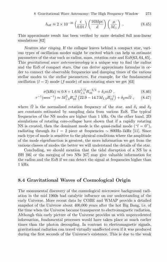
8 Gravitational Wave Astronomy: The High Frequency Window 273
heff ≈ 2 × 10⁻²¹( ε
0.01
)(10Mpcd
)(µ
M
). (8.45)
This approximate result has been verified by more detailed full non-linearsimulations [62]
Neutron star ringing. If the collapse leaves behind a compact star, vari-ous types of oscillation modes might be excited which can help us estimateparameters of the star such as radius, mass, rotation rate and EoS[63, 64, 65].This gravitational wave asteroseismology is a unique way to find the radiusand the EoS of compact stars. One can derive approximate formulas in or-der to connect the observable frequencies and damping times of the variousstellar modes to the stellar parameters. For example, for the fundamentaloscillation (l = 2) mode (f -mode) of non-rotating stars we get [63]
σ(kHz) ≈ 0.8 + 1.6M1/21.4 R
−3/210 + δ1mΩ , (8.46)
τ−1(secs−1) ≈ M31.4R
−410
(22.9 − 14.7M1.4R
−110
)+ δ2mΩ , (8.47)
where Ω is the normalized rotation frequency of the star, and δ1 and δ2are constants estimated by sampling data from various EoS. The typicalfrequencies of the NS modes are higher than 1 kHz. On the other hand, 2Dsimulations of rotating core-collapse have shown that if a rapidly rotatingNS is created, then the dominant mode is the quasi-radial mode (“l = 0”),radiating through its l = 2 piece at frequencies ∼ 800Hz-1kHz [11]. Sinceeach type of mode is sensitive to the physical conditions where the amplitudeof the mode eigenfunction is greatest, the more information we get from thevarious classes of modes the better we will understand the details of the star.
Concluding, we should mention that the tidal disruption of a NS by aBH [66] or the merging of two NSs [67] may give valuable information forthe radius and the EoS if we can detect the signal at frequencies higher than1 kHz.
8.4 Gravitational Waves of Cosmological Origin
The monumental discovery of the cosmological microwave background radi-ation in the mid 1960s had catalytic influence on our understanding of theearly Universe. More recent data by COBE and WMAP provide a detailedsnapshot of the Universe about 400,000 years after the hot Big Bang, i.e. ofthe time when the Universe became transparent to electromagnetic radiation.Although this early picture of the Universe provides us with unprecedentedinformation, fundamental processes would have taken place at much earliertimes than the photon decoupling. In contrast to electromagnetic signals,gravitational radiation can travel virtually unaffected even if it was producedduring the first seconds of the Universe’s existence. This is due to the weak
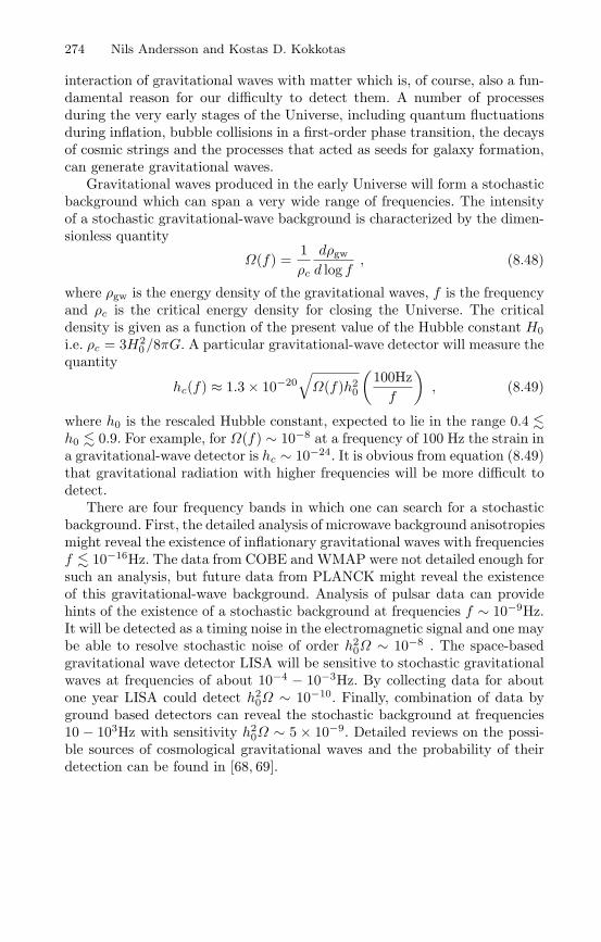
274 Nils Andersson and Kostas D. Kokkotas
interaction of gravitational waves with matter which is, of course, also a fun-damental reason for our difficulty to detect them. A number of processesduring the very early stages of the Universe, including quantum fluctuationsduring inflation, bubble collisions in a first-order phase transition, the decaysof cosmic strings and the processes that acted as seeds for galaxy formation,can generate gravitational waves.
Gravitational waves produced in the early Universe will form a stochasticbackground which can span a very wide range of frequencies. The intensityof a stochastic gravitational-wave background is characterized by the dimen-sionless quantity
Ω(f) =1ρc
dρgwd log f
, (8.48)
where ρgw is the energy density of the gravitational waves, f is the frequencyand ρc is the critical energy density for closing the Universe. The criticaldensity is given as a function of the present value of the Hubble constant H0i.e. ρc = 3H2
0/8πG. A particular gravitational-wave detector will measure thequantity
hc(f) ≈ 1.3 × 10⁻²⁰√Ω(f)h2
0
(100Hzf
), (8.49)
where h0 is the rescaled Hubble constant, expected to lie in the range 0.4 h0 0.9. For example, for Ω(f) ∼ 10−8 at a frequency of 100 Hz the strain ina gravitational-wave detector is hc ∼ 10−24. It is obvious from equation (8.49)that gravitational radiation with higher frequencies will be more difficult todetect.
There are four frequency bands in which one can search for a stochasticbackground. First, the detailed analysis of microwave background anisotropiesmight reveal the existence of inflationary gravitational waves with frequenciesf 10−16Hz. The data from COBE and WMAP were not detailed enough forsuch an analysis, but future data from PLANCK might reveal the existenceof this gravitational-wave background. Analysis of pulsar data can providehints of the existence of a stochastic background at frequencies f ∼ 10−9Hz.It will be detected as a timing noise in the electromagnetic signal and one maybe able to resolve stochastic noise of order h2
0Ω ∼ 10−8 . The space-basedgravitational wave detector LISA will be sensitive to stochastic gravitationalwaves at frequencies of about 10−4 − 10−3Hz. By collecting data for aboutone year LISA could detect h2
0Ω ∼ 10−10. Finally, combination of data byground based detectors can reveal the stochastic background at frequencies10 − 103Hz with sensitivity h2
0Ω ∼ 5 × 10⁻⁹. Detailed reviews on the possi-ble sources of cosmological gravitational waves and the probability of theirdetection can be found in [68, 69].
8 Gravitational Wave Astronomy: The High Frequency Window 275
Acknowledgements
This work has been supported by the EU Programme ’Improving the Hu-man Research Potential and the Socio-Economic Knowledge Base’ (ResearchTraining Network Contract HPRN-CT-2000-00137). KK acknowledges sup-port throught the Center of Gravitational Wave Physics, which is funded bythe NSF number cooperative agreement PHY 01-14375.
References
1. C. Cutler, K.S. Thorne, in proceedings of GR16 (Durban South Africa, 2001),gr-qc/0204090.
2. R. Schnabel, J. Harms, K.A Strain, K. Danzmann, Class. Quantum Grav. 21,S1155 (2004).
3. M. Bonaldi, M. Cerdonio, L. Conti, G.A. Prodi, L. Taffarello, J.P. Zendri,Class. Quantum Grav. 21, S1155 (2004).
4. M. Burgay, N. D’Amico, A. Possenti, R.N. Manchester, A.G. Lyne, B.C. Joshi,M.A. McLaughlin, M. Kramer, J.M. Sarkissian, F. Camilo, V. Kalogera,C. Kim, D.R. Lorimer, Nature, 426, 531 (2003).
5. V. Kalogera, C. Kim, D.R. Lorimer, M. Burgay, N. D’Amico, A. Possenti,R.N. Manchester, A.G. Lyne, B.C. Joshi, M.A. McLaughlin, M. Kramer,J.M. Sarkissian, F. Camilo, Astrophys.J. 601, L179 (2004).
6. E. Cappellaro, M. Turatto, D.Yu. Tsvetov, O.S. Bartunov, C. Pollas, R. Evansand M. Hamuy, A&A 351, 459 (1999).
7. O. Zanotti, L. Rezzolla, J. A. Font, M.N.R.A.S., 341 832 (2003).8. C.L. Fryer, S.E. Woosley, A. Heger, Astrophys. J. 550, 372 (2001).9. C.L. Fryer, V. Kalogera, Astrophys. J. 554, 548 (2001).
10. C.L. Fryer, A. Heger, Astrophys. J. 541 1033 (2000).11. H. Dimmelmeier, J.A. Font, E. Muller, A& A 393, 523 (2002).12. S.L. Finn, C.R. Evans, Astrophys. J, 351, 588 (1990).13. T. Zwerger, E. Muller, A & A 320, 209 (1997).14. M. Rampp, E. Muller, M. Ruffert, A& A 332, 969 (1998).15. C.L. Fryer, D.E. Holz, S.A. Hudges, Astrophys. J. 565, 430 (2002).16. C.D. Ott, A. Burrows, E. Livne, R. Walder, Astrophys. J. 600, 834 (2004).17. K. Kotake, S. Yamada, K. Sato K, Phys. Rev. D 68, 044023 (2003).18. M. Shibata, Astrophys. J. 595, 992 (2003).19. L. Baiotti, I. Hawke, P. . Montero, F. Loffler, L. Rezzolla, N. Stergioulas, J.
A. Font, E. Seidel, gr-qc/0403029.20. P.A. Caraveo, Astrophys. J. 415, L111 (1993).21. A. Burrows, J. Hayes, Phys. Rev. Lett. 76, 1037 (1996).22. E. Muller, H.-Th. Janka, A& A 317, 140 (1997).23. H. C. Spruit, E.S. Phinney, Nature 393, 139 (1998).24. L. C. Loveridge, Phys. Rev. D 69,024008 (2004).25. P. Hoeflich, A. Khokhlov, L. Wang, J. C. Wheeler, D. Baade, IAU Symposium
212 on Massive Stars, D. Reidel Conf. Series, ed. E. van den Hucht, astro-ph/0207272.
26. Y. T Liu, L. Lindblom, M.N.R.A.S. 324, 1063 (2001).
276 Nils Andersson and Kostas D. Kokkotas
27. S. Kobayasi, P. Meszaros, Astrophys. J. 589,861 (2003).28. M. Shibata, T. W. Baumgarte, S. L. Shapiro, Astrophys. J. 542, 453 (2000).29. J. M. Centrella, K. C. B. New, L.L. Lowe, J.D. Brown, Astrophys. J. Lett. 550
193 (2001).30. M. Shibata, S. Karino, Y. Eriguchi, M.N.R.A.S. 334, L27 (2002).31. M. Shibata, S. Karino, Y. Eriguchi, M.N.R.A.S. 343, 619 (2003).32. M. Saijo, T. W. Baumgarte, S. L. Shapiro, Astrophys. J. 595, 352 (2002).33. K.D. Kokkotas, J. Ruoff, N. Andersson: gr-qc/021241934. S. Chandrasekhar, Phys. Rev. Lett. 24, 611 (1970).35. J.L. Friedman, B.F. Schutz, Astroph. J. 222, 281 (1978).36. N. Stergioulas, J.L. Friedman, Astrophys. J. 492, 301 (1998).37. S. Yoshida, L. Rezzolla, S. Karino, Y. Eriguchi, Astrophys. J. Lett. 568, 41
(2002).38. N. Stergioulas, Living Reviews in Relativity 6 3 (2003).39. D. Lai, S.L. Shapiro, Astrophys. J. 442, 259 (1995).40. L. Lindblom, B. J. Owen, S. M. Morsink, Phys. Rev. Lett., 80 4843 (1998).41. B. Owen, L. Lindblom, C. Cutler, B.F. Schutz, A. Vecchio, N. Andersson,
Phys. Rev. D 58, 084020 (1998).42. N. Andersson, K. D. Kokkotas, B. F. Schutz, Astrophys. J. 510, 846 (1999).43. L. Bildsten, G. Ushomirsky, Astrophys. J. 529, L33 (2000).44. L. Lindblom, B. J. Owen, G. Ushomirsky, Phys. Rev. D 62, 084030 (2000).45. A. K. Schenk, P. Arras, E.E. Flanagan, S.A. Teukolsky, I. Wasserman,
Phys. Rev. D 65, 024001 (2002).46. L. Rezzolla, F. K. Lamb, S. L. Shapiro, Astrophys. J. 531, L139 (2000).47. L. Lindblom, B. Owen, Phys. Rev. D 65, 063006 (2002).48. N. Andersson and K. D. Kokkotas, I.J.M.P. D10,381 (2001).49. N. Andersson, Class. Quantum Grav., 20 R105 (2003).50. N. Andersson, K. D. Kokkotas, N. Stergioulas, Astrophys. J. 307, 314 (1999).51. N. Andersson, D.I. Jones, K.D. Kokkotas, N. Stergioulas, Astrophys. J. Lett.
534 L75 (2000).52. J. Heyl, Astrophys. J. Lett. 574 L57 (2002).53. R.V. Wagoner, Astrophys. J. Lett. 578 L63 (2002).54. N. Andersson, D.I. Jones, K. D. Kokkotas, M.N.R.A.S. 337 1224 (2002).55. A. Reisenegger, A. Bonacic, Phys. Rev. Lett. 91, 201103 (2003).56. R.A. Araya-Gochez astro-ph/031100157. A. Nagar, G. Diaz, J. A. Pons, J. A. Font, gr-qc/0403077.58. E. Echeverria, Phys. Rev. D 40 3194 (1988).59. L.S. Finn, Phys. Rev. D 8 3308 (1992).60. O. Dryer, B. Kelly, B. Krishnan, L. S. Finn, D. Garrison, R. Lopez-Aleman,
Class. Quantum Grav. 21, 787 (2004).61. M. Davis, R. Ruffini, W.H. Press, R.H. Price, Phys. Rev. Lett.27, 1466 (1971).62. P. Anninos, R. H. Price, J. Pullin, E. Seidel, W.-M. Suen, Phys. Rev. D 52,
4462 (1995).63. N. Andersson, K.D. Kokkotas, M.N.R.A.S. 299, 1059 (1998).64. K.D. Kokkotas, T. Apostolatos, N. Andersson, M.N.R.A.S. 320 307 (2001).65. N. Andersson, G.L. Comer, Phys. Rev. Lett.87, 241101 (2001).66. M. Vallisneri, Phys. Rev. Lett. 84 3519 (2000).67. J.A. Faber, P. Grandclement, F.A. Rasio, K. Taniguchi, Phys. Rev. Lett. 89
231102 (2002).68. B. Allen in Les Houches School on Astrophysicsl Sources of Gravitational
Waves, eds J.A. Marcka and J.P. Lasota, Cambridge University Press (1996).69. M. Maggiore, Phys. Reports 331, 283 (2000).
9 Computational Black Hole Dynamics
Pablo Laguna1 and Deirdre M. Shoemaker2
1 Department of Astronomy and Astrophysics, Institute for Gravitational Physicsand Geometry, Center for Gravitational Wave Physics, Penn State University,University Park, PA 16802, USA
2 Center for Radiophysics and Space Research, Cornell University, Ithaca, NY14853, USA
Abstract. Over the last decade, advances in computer hardware and numericalalgorithms have opened the door to the possibility that simulations of sources ofgravitational radiation can produce valuable information of direct relevance to grav-itational wave astronomy. One source in particular is believed to be of extremeimportance: the inspiral and merger of a binary black hole system. Simulations ofbinary black hole systems involve solving the Einstein equation in full generality.Such a daunting task has been one of the primary goals of the numerical relativitycommunity. This review article focuses on the computational modelling of binaryblack holes. It provides a basic introduction to the subject and is intended fornon-experts in the area of numerical relativity.
9.1 Introduction
A new era in astronomy will begin once gravitational wave interferometerssuch as LIGO, GEO, VIRGO, TAMA and, in the future, LISA detect firstlight. It is expected that these detectors will provide a revolutionary view ofthe Universe, complementary to the electromagnetic perspective. In this newastronomy, the messengers are gravitational waves, ripples in the fabric ofspacetime. These waves will have encoded detailed knowledge of the coher-ent, bulk motions of matter and the vibrations in the curvature of spacetimeproduced by a vast class of astrophysical sources; compact object binaries,supernovae, spinning neutron stars, gamma ray bursts and stochastic back-grounds are just a few examples of these sources.
Detection of the stochastic background of gravitational waves will revo-lutionize early universe cosmology and high energy physics by tapping intoinformation unaccessible by any other means. Because gravitational wavesinteract so weakly, they penetrate much deeper into the universe and its his-tory. If these relic gravitational waves are observed, they will have imprintedon them a snapshot of the very early universe at the time when they weredecoupled from the primordial plasma. This will provide the means to investi-gate the origins of the universe and to measure cosmological parameters froma new perspective. A summary of how ground based gravitational wave detec-tors do cosmology can be found in [1]. This topic is of such importance thatNASA has developed a program to investigate it called “Beyond Einstein”,details at http://universe.gsfc.nasa.gov/.
P. Laguna and D.M. Shoemaker, Computational Black Hole Dynamics, Lect. Notes Phys. 653,277–298 (2005)http://www.springerlink.com/ c© Springer-Verlag Berlin Heidelberg 2005

278 Pablo Laguna and Deirdre M. Shoemaker
The same reason that gravitational waves have such a long-reach in timeand space is the reason they are so difficult to detect. The detection is aformidable undertaking, requiring innovative engineering, powerful data anal-ysis tools and careful theoretical modelling. Our article focuses on the com-putational modelling of binary black holes. It provides a basic introductionto the subject and is intended for non-experts in the area of numerical rel-ativity. The article is an expanded version of the lecture notes given by oneof us at the Second Aegean Summer School. For a comprehensive review, werecommend the one by Baumgarte and Shapiro [2].
Among the sources of gravitational radiation, binary systems consistingof black holes and/or neutron stars are expected to play a dominant role [3].Over the last couple of decades, advances in numerical algorithms and com-puter hardware have increased the impact that constructing numerical solu-tions of the Einstein equation has on astrophysical systems such as black-holebinaries. The ultimate goal is to develop generic numerical codes that, giveninitial data and boundary conditions, will produce a spacetime representingmultiple black-hole singularities. The hope is that these codes will be capableof modeling the dynamics of a binary black-hole collision, including inspiral,merger, and ringdown phases.
This article is divided as follows: In Sect. 9.2 we presents the traditionalintroduction to the (3+1) decomposition of the Einstein equation. Since theprimary focus is on black hole spacetimes, we will concentrate on the vac-uum case. Also in this section, we will briefly discuss the two most popular(3+1) formulations currently used by the numerical relativity community.Section 9.3 is dedicated to black-hole horizons and the infrastructure devel-oped around them that is used in numerical simulations. In particular, we willdescribe the excision method to handle black hole singularities. In Sect. 9.4,we review the Kerr-Schild form of a single black-hole spacetime and its use asa building block for numerical evolutions. In Sect. 9.5, we review the currentstatus of black-hole simulations. Conclusions and a look at what lies aheadin the near future are given in Sect. 9.6.
9.2 Einstein Equation and Numerical Relativity
The essence of Einstein equation is the notion that geometry is related tomatter-energy. Specifically,
Gab = 8πTab , (9.1)
where Gab is the Einstein tensor (geometry) and Tab is the stress-energytensor (matter-energy). The Einstein tensor Gab is an operator acting onthe spacetime metric (4)gab. This operator is nonlinear, involving first andsecond derivatives of the metric. Since this review focuses on black holes, wewill concentrate on vacuum spacetimes and thus set Tab = 0. Also, Latin
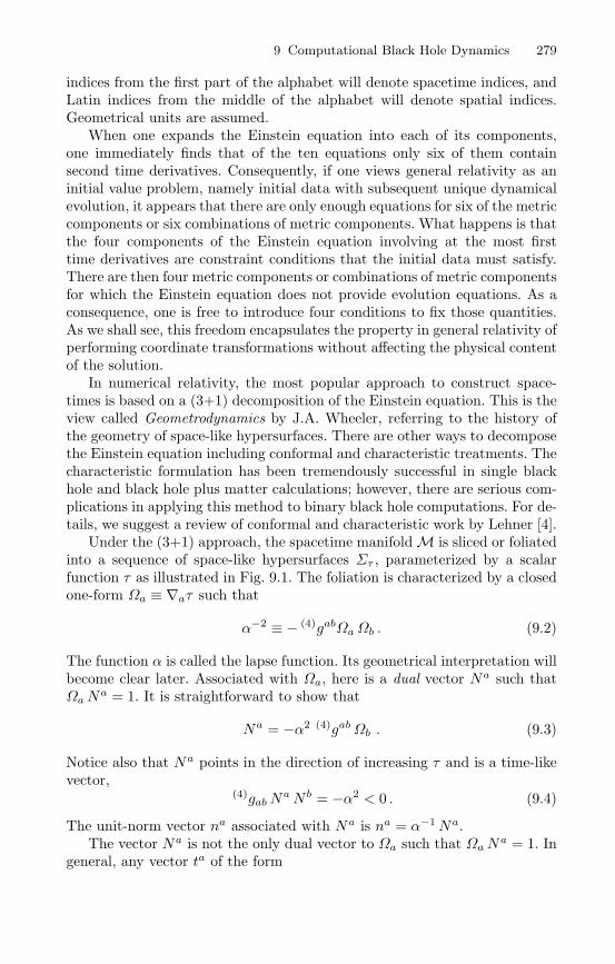
9 Computational Black Hole Dynamics 279
indices from the first part of the alphabet will denote spacetime indices, andLatin indices from the middle of the alphabet will denote spatial indices.Geometrical units are assumed.
When one expands the Einstein equation into each of its components,one immediately finds that of the ten equations only six of them containsecond time derivatives. Consequently, if one views general relativity as aninitial value problem, namely initial data with subsequent unique dynamicalevolution, it appears that there are only enough equations for six of the metriccomponents or six combinations of metric components. What happens is thatthe four components of the Einstein equation involving at the most firsttime derivatives are constraint conditions that the initial data must satisfy.There are then four metric components or combinations of metric componentsfor which the Einstein equation does not provide evolution equations. As aconsequence, one is free to introduce four conditions to fix those quantities.As we shall see, this freedom encapsulates the property in general relativity ofperforming coordinate transformations without affecting the physical contentof the solution.
In numerical relativity, the most popular approach to construct space-times is based on a (3+1) decomposition of the Einstein equation. This is theview called Geometrodynamics by J.A. Wheeler, referring to the history ofthe geometry of space-like hypersurfaces. There are other ways to decomposethe Einstein equation including conformal and characteristic treatments. Thecharacteristic formulation has been tremendously successful in single blackhole and black hole plus matter calculations; however, there are serious com-plications in applying this method to binary black hole computations. For de-tails, we suggest a review of conformal and characteristic work by Lehner [4].
Under the (3+1) approach, the spacetime manifold M is sliced or foliatedinto a sequence of space-like hypersurfaces Στ , parameterized by a scalarfunction τ as illustrated in Fig. 9.1. The foliation is characterized by a closedone-form Ωa ≡ ∇aτ such that
α−2 ≡ − (4)gabΩaΩb . (9.2)
The function α is called the lapse function. Its geometrical interpretation willbecome clear later. Associated with Ωa, here is a dual vector Na such thatΩaN
a = 1. It is straightforward to show that
Na = −α2 (4)gabΩb . (9.3)
Notice also that Na points in the direction of increasing τ and is a time-likevector,
(4)gabNaN b = −α2 < 0 . (9.4)
The unit-norm vector na associated with Na is na = α−1Na.The vector Na is not the only dual vector to Ωa such that ΩaN
a = 1. Ingeneral, any vector ta of the form
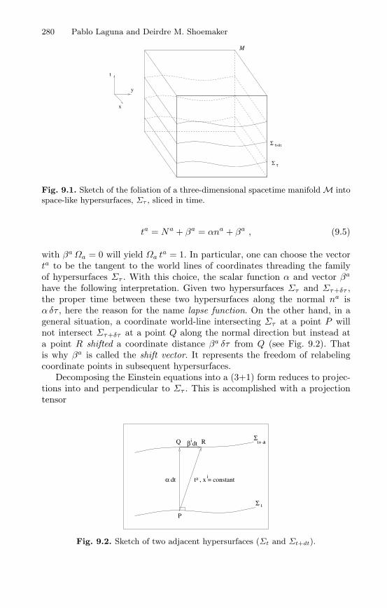
280 Pablo Laguna and Deirdre M. Shoemaker
t
M
+δττΣ
y
x
Σ τ
Fig. 9.1. Sketch of the foliation of a three-dimensional spacetime manifold M intospace-like hypersurfaces, Στ , sliced in time.
ta = Na + βa = αna + βa , (9.5)
with βaΩa = 0 will yield Ωa ta = 1. In particular, one can choose the vector
ta to be the tangent to the world lines of coordinates threading the familyof hypersurfaces Στ . With this choice, the scalar function α and vector βa
have the following interpretation. Given two hypersurfaces Στ and Στ+δτ ,the proper time between these two hypersurfaces along the normal na isα δτ , here the reason for the name lapse function. On the other hand, in ageneral situation, a coordinate world-line intersecting Στ at a point P willnot intersect Στ+δτ at a point Q along the normal direction but instead ata point R shifted a coordinate distance βa δτ from Q (see Fig. 9.2). Thatis why βa is called the shift vector. It represents the freedom of relabelingcoordinate points in subsequent hypersurfaces.
Decomposing the Einstein equations into a (3+1) form reduces to projec-tions into and perpendicular to Στ . This is accomplished with a projectiontensor
, x = constant
d iβ
atdt i
RQ
P
dt tt+
t
α
Σ
Σ
Fig. 9.2. Sketch of two adjacent hypersurfaces (Σt and Σt+dt).

9 Computational Black Hole Dynamics 281
⊥ab ≡ δab + nanb . (9.6)
Notice that by construction ⊥ab n
b = 0. For instance, given an arbitrarytensor T ....
..a.., the projection of the covariant index a is accomplished by⊥b
a T....
..b.., and similarly for other indices. The notation ⊥ preceding atensor implies projecting every free index in the tensor. In particular, theprojection of the spacetime metric is
gab ≡⊥ (4)gab = ⊥ca ⊥d
b(4)gcd = (4)gab + na nb . (9.7)
The tensor gab is the intrinsic metric to Στ . Because gab and βa are tensorsin Στ , one can also write gij = gab as well as βi = βa. The spacetime metricgiven as a line element can then be decomposed as follows:
ds2 = −α2dt2 + gij(dxi + βidt)(dxj + βjdt) . (9.8)
The spatial metric gab induces a covariant differentiation operator Da inΣτ . That is, Dagab = 0 with Da =⊥ ∇a. For instance
DaTb1...bl
c1...cm= ⊥b1
d1 . . .⊥bldl
⊥e1c1 . . .⊥em
cm⊥f
a∇fTd1...dl
e1...em.(9.9)
In order to completely characterize the spacetime from the point of viewof the (3+1) decomposition, it is not enough to have the intrinsic metric gab.One needs in addition information on how the hypersurfaces are embeddedin the spacetime, namely the extrinsic curvature Kab of Στ . The extrinsiccurvature is defined as
Kab = − ⊥ ∇(anb) = −12
⊥ Lngab = −12Ln
(4)gab , (9.10)
where Ln is the Lie derivative along the normal na. It is not difficult to showthat
Kab = −∇anb − na ab , (9.11)
where ab = na∇anb is the 4-acceleration of coordinate observers.
Finally, given an arbitrary vectorW a inΣτ , the curvature Riemann tensorRabc
d is defined via the action of Da on Wa as:
(DaDb −DbDa)Wc = RabcdWd . (9.12)
Similarly, the spatial Ricci tensor Rab and the spatial Ricci scalar R areobtained from Rab = Racb
c and R = Raa, respectively.
The relation between the curvature tensor Rabcd of the spacetime manifoldM and the curvature tensor Rabcd of hypersurface manifold Στ is given bythe Gauss, Codazzi and Ricci equations:
⊥ Rabcd = Rabcd +KacKbd −KadKbc (9.13)⊥ Rabcn = DaKac −DaKbc (9.14)
⊥ Ranbn = LnKab +1αDaDb α+Ka
cKab , (9.15)

282 Pablo Laguna and Deirdre M. Shoemaker
where we have used the following notation
na T ......a.. ≡ T ....
..n.. . (9.16)
We are now in the position of considering the decomposition of the Ein-stein tensor Gab = Rab − gab R/2. Without loss of generality, this tensor canbe rewritten as:
Gab =⊥ Gab − 2n(a ⊥ Gb)n + nanbGnn . (9.17)
With the help of (9.13), it becomes
2Gnn = R+K2 −KabK
ba . (9.18)
Similarly, making use of (9.14), one obtains
⊥ Gan = −DbKab +DaK . (9.19)
The next step would be to write ⊥ Gab in terms of (3+1) quantities. However,as originally pointed out by York [5], it is more convenient to use ⊥ Rab
instead. A straightforward but tedious calculation yields
⊥ Rab = LnKab +1αDaDb α+ 2Ka
cKcb −KKab −Rab . (9.20)
Note that (9.18–9.20) involve only spatial tensors; therefore, they can equallybe written with spatial indices.
Since we are interested in the vacuum case, the Einstein equation simplyreads Gab = 0. Equations (9.18–9.20) reduce to
R+K2 −KijK
ji = 0 (9.21)
DjKij −DiK = 0 (9.22)∂oKij = −DiDjα+ α (Rij +KKij − 2KilK
lj) (9.23)
∂ogij = −2αKij , (9.24)
where we have introduced the following notation: ∂o ≡ ∂t − Lβ . Notice alsothat we have added (9.24), which is basically the definition of the extrinsiccurvature (see (9.10)).
Equations (9.21) and (9.22) are known as the Hamiltonian and momentumconstraints. Equations (9.23) and (9.24) are also known as the K-dot and g-dotequations or the ADM evolution equations. The ADM name was originatedbecause of the work on (3+1) decompositions of the Einstein equation byArnowitt, Deser, and Misner [6]. Strictly speaking calling (9.23) and (9.24)the ADM equations is incorrect. The equations derived by Arnowitt, Deser,and Misner use a extrinsic curvature density and the evolution equation forthe densitized extrinsic curvature is derived from ⊥ Gab. To our knowledge,the system (9.21-9.24) as it stands was first introduced by York [5].
The traditional approach in numerical relativity to solve the system ofequations (9.21-9.24) for spacetimes containing black hole singularities re-quires the following action items:
9 Computational Black Hole Dynamics 283
– Specify spatial coordinates xi (e.g. Cartesian, spherical, etc.) and topol-ogy of the initial slice.
– Construct initial data gij , Kij such that the constraints (9.21) and(9.22) are satisfied.
– Prescribe a recipe to fix α and βi.– Impose boundary conditions.– Handling black hole singularities.– Evolve or update in time the data gij , Kij via (9.23) and (9.24).
There are of course a series of important and complicated issues in han-dling each of the items above. For instance regarding initial data, there aretwelve quantities in gij , Kij but only four constraint equations. How dowe select among these twelve quantities those that are derived from the con-straints? York and collaborators [5], based on earlier work by Lichnerowicz,developed an extremely powerful methodology that singles out those piecesin gij , Kij that are to be obtained from the constraints (9.21) and (9.22).This method is commonly known as the York conformal approach to the ini-tial data problem in general relativity. For an excellent review and modernvariations, we encourage the reader to look at the review by Cook [7].
Similarly, there are important aspects to be considered in the choice ofthe gauge variables α and βi as well as boundary conditions. Throughout thevarious disciplines of physics, boundary conditions are often one of the mostdemanding aspects. Recently in numerical relativity, a great deal of atten-tion has been devoted to boundary conditions that are constraint preserving[8]. This work is attempting to relieve the prevalence of constraint violationduring evolutions by applying explicit constraint preserving boundary condi-tions. Regarding the choice of the lapse and the shift, the numerical relativitycommunity seems to be converging on gauge condition of the driver type [9].The idea behind these gauge condition is to design evolution equations foralpha and βi that drive certain quantities to a steady state. These conditionshave been successfully used in both black hole and neutron star calculations.
The most common procedure to evolve initial data in numerical relativityis the so called free evolution. In a free evolution, the constraint equations areonly used to monitor the quality of the evolved data, namely the departures ofthe numerically data from satisfying the constraints. Because of truncation ordiscretization errors, the evolved data will satisfy at best the discrete versionof the constraints. More often, these errors drive the solutions rapidly awayfrom the constraint surface, rendering the simulation unstable. It is fair to saythat one of the primary tasks in numerical relativity has been the control ofthese constraint violating modes [10, 11]. Recently there have been attemptsto explicitly solve the constraints as a way of projecting the evolved databack into the constraint surface [12].
The ADM formulation is not unique. There are in principle an infinitenumber of ways of formulating the Einstein equation with a (3+1) structure.One can simply add terms to the evolution equations involving the constraints
284 Pablo Laguna and Deirdre M. Shoemaker
to create a different set of evolution equations. For instance,
∂ogij = r.h.s. Eq. (9.24) + Pij ρ+ Ukij Jk (9.25)
∂oKij = r.h.s. Eq. (9.23) +Qij ρ+ V kij Jk , (9.26)
where
ρ ≡ R+K2 −KijK
ji (9.27)
J i ≡ DjKij −DiK . (9.28)
Above, Pij , Qij , Ukij and V k
ij are tensors, symmetric in the ij indices in-volving parameters as well as metric functions [13]. These types of adjustmenthave a deep impact on the well-posedness properties of the system. Amongall the formulations that have been proposed, there are two that are cur-rently enjoying widespread popularity. We will quickly summarize both. Foran extensive review on hyperbolic formulations of the Einstein equation thereader should consult Reula’s review [14].
The first of the two formulations is the so called BSSN system. This isa formulation re-introduced by Baumgarte and Shapiro [15] and originallydeveloped by Shibata and Nakamura [16]. The first step in obtaining theBSSN formulation is to abandon gij and Kij as primary variables and workinstead with Φ, gij , K and Aij . The relationships between these and theADM variables are
Φ =16
ln g1/2 (9.29)
gij = e−4Φ gij (9.30)
Aij = e−4ΦAij , (9.31)
where Aij = Kij − gij K/3. Given (9.29)-(9.31), it is not difficult to showthat the ADM system of evolution equations take the form
∂oΦ = −16αK (9.32)
∂ogij = −2α Aij (9.33)
∂oK = −∇i∇iα+ α (AijAij +K2/3) (9.34)
∂oAij = e−4Φ (−∇i∇jα+ αRij)TF
+ α (KAij − 2AilAlj) . (9.35)
where in (9.35) the superscript TF denotes the trace free part of the tensorbetween brackets, e.g. TTF
ij ≡ Tij − gijgklTkl/3 for any tensor Tij . The keyingredient of the BSSN system is the introduction of a conformal connection
Γ i ≡ gjkΓ ijk = −∂j g
ij , (9.36)

9 Computational Black Hole Dynamics 285
where the Γ ijk are the connection coefficients associated with gij . The moti-
vation for introducing these connections is to substitute in the Ricci tensorRij all the derivatives of gjkΓ i
jk in favor of derivatives of Γ i. In doing so, theRicci tensor yields a system of evolution equations with a hyperbolic flavor.
Expanding the number of primary variables in the system to include theconformal connections implies the need of an additional evolution equation.From definition (9.36), one can show that the evolution equation for Γ i isgiven by
∂oΓi = gjk∂jkβ
i +13gij∂jkβ
k − 2 Aij∂jα
+ 2αΓ ijkA
jk + 12αAij∂jΦ− 43α∇iK . (9.37)
In summary, the BSSN system involves conformal transformations, a trace-free decomposition of the extrinsic curvature, the introduction of a conformalconnection and the use of constraints to eliminate the Ricci scalar and deriva-tives of the trace-free extrinsic curvature.
The other currently most popular (3+1) formulation of the Einstein equa-tion is the KST formulation developed by Kidder, Scheel and Teukolsky [17].There are a number of ways to construct hyperbolic formulations [14], butwe only include the KST formulation in any detail. Strictly speaking this is afamily of hyperbolic formulations foliated by twelve parameters. This formu-lation has been demonstrated to be successful in the evolution of single blackholes. It is expected that in the near future this success will be translated toevolutions of binary black holes.
The first step in the derivation of the KST system consists of introducinga new variable to eliminate second derivatives of the spatial metric. The newvariable (symmetric on its last two indices) is
dkij ≡ ∂kgij , (9.38)
and its traces dk ≡ gijdkij and bk ≡ gijdijk. An evolution equation for dkij
is obtained by taking a spatial derivative of (9.24). This yields
∂odkij = −2α∂kKij − 2Kij∂kα . (9.39)
In terms of the new variables, the evolution equation for the extrinsic curva-ture becomes
∂oKij = α[12gkl(∂(idklj) + ∂kd(ij)l − ∂kdlij − ∂(idj)kl
)
+12bkdkij − 1
4dkdkij − bkd(ij)k − 1
2d l
kj dk
li
+12dkd(ij)k +
14d kl
i djkl +12dkl
idklj − 2KikKk
j
+KKij
]− ∂i∂jα− 1
2dk
ij∂kα+ d k(ij) ∂kα .
286 Pablo Laguna and Deirdre M. Shoemaker
By adding terms proportional to the constraints, the evolution equationsfor Kij and dkij can be rewritten as
∂oKij = (. . .) + γαgijC + ζαgklCk(ij)l (9.40)∂odkij = (. . .) + ηαgk(iCj) + χαgijCk , (9.41)
where (. . .) represents the right-hand side of either (9.39) or (9.40). Theparameters γ, ζ, η, χ are arbitrary constants. The evolution equations arenow given by
∂ogij 0, (9.42)
∂oKij −12αgkl
[∂kdlij − (1 + ζ)∂kd(ij)l
− (1 − ζ)∂(idklj) + (1 + 2σ)∂(idj)kl
−γgijgmn∂kdmnl + γgijgmn∂kdlmn] , (9.43)∂odkij −2α∂kKij + αglm
(ηgk(i∂lKmj) + χgij∂lKmk
−ηgk(i∂j)Klm − χgij∂kKlm
), (9.44)
where denotes equal to the principal part. In [17] it is shown that one canfind values of the parameters such that the system is weakly hyperbolic. Itis also found that densitizing the lapse is a necessary condition for stronghyperbolicity, namely:
α = gσ eQ , (9.45)
with Q an arbitrary function and σ a parameter.Finally, in order to arrive at the KST system, one introduces a generalized
extrinsic curvature Pij using the relation
Pij ≡ Kij + zgijK , (9.46)
where z is an arbitrary parameter. Similarly one introduces a generalizedderivative of the metric, Mkij , using the relation
Mkij =12
kdkij + ed(ij)k + gij
[adk + bbk
]
+gk(i
[cdj) + dbj)
], (9.47)
with k, e, a, b, c and d additional parameters. With these definitions, theprincipal parts of the evolution equations for Pij and Mkij are
∂ogij 0 (9.48)∂oPij −αgkl
(µ1∂kMlij + µ2∂kM(ij)l + µ3∂(iMklj)
+ µ4∂(iMj)kl + µ5gijgmn∂kMmnl
+µ6gijgmn∂kMlmn) (9.49)
∂oMkij −α (ν1∂kPij + ν2∂(iPj)k + ν3gmngk(i∂mPnj)
+ ν4gijgmn∂mPnk + ν5gmngk(i∂j)Pmn
+ν6gijgmn∂kPmn) , (9.50)

9 Computational Black Hole Dynamics 287
where µA and νA with A = 1...6 are parameters function of the 12 parametersabove.
9.3 Black Hole Horizons and Excision
Back hole horizons are of crucial importance in numerical simulations thatmay either contain or lead to the formation of black holes. Specifically innumerical relativity, horizons are used to identify the formation of a blackhole, to locate a black hole or to characterize properties of a black hole.To successfully utilize horizons in computations, they must be formulated interms appropriate to numerical approximations. We will briefly review thetypes of black hole horizons that have been used in connection with numericalsimulations.
A black hole is most often defined in terms of its event horizon, i.e. thefuture boundary of the causal past of future null infinity. The event horizonis a mathematically elegant and powerful definition of the black hole surface;however, for the purposes of locating in a numerical simulation the positionof the black hole in the computational domain this definition is not alwaysuseful. By definition, the event horizon is global in nature; meaning, theentire spacetime must be known a priori in order to determine its location.This is demanding the end product of the evolution before we even begin. Inpractice, an alternative surface called apparent horizon is used to localize ortrack the position of a black hole.
An apparent horizon is a closed two-sphere on Στ . Therefore, it is wellsuited for numerical relativity since it only requires information available atan instant of time. There is a price to pay however. Because they are definedfrom quantities in Στ , they dependent on the way one chooses to foliate thespacetime. One can in principle find foliations of a black hole spacetime inwhich a hypersurface Στ does not contain an apparent horizon. Fortunately,these type of slicings seem to be rare. Furthermore, the world tube connectingapparent horizons from one time to the next could be discontinuous. This isin contrast with an event horizon which is a continuous worldtube.
The apparent horizon is defined as the outermost marginally trappedsurface in Στ . As mentioned before, the definition of an apparent horizonrequires only knowledge of quantities on Στ . Following [18], let S be a surfacewith S2 topology with ka and la respectively the outgoing and ingoing nullvectors to S, see Fig. 9.3. That is, kasa > 0 and lasa < 0, where sa is aspacelike unit vector to S in Στ , namely sana = 0 with na the unit time-likenormal to Στ .
A trapped surface is defined as
Θ ≡ ∇aka ≤ 0 . (9.51)
By making use of ka = na + sa and the projector ⊥, (9.51) can be rewrittenin terms of quantities on Στ as follows:
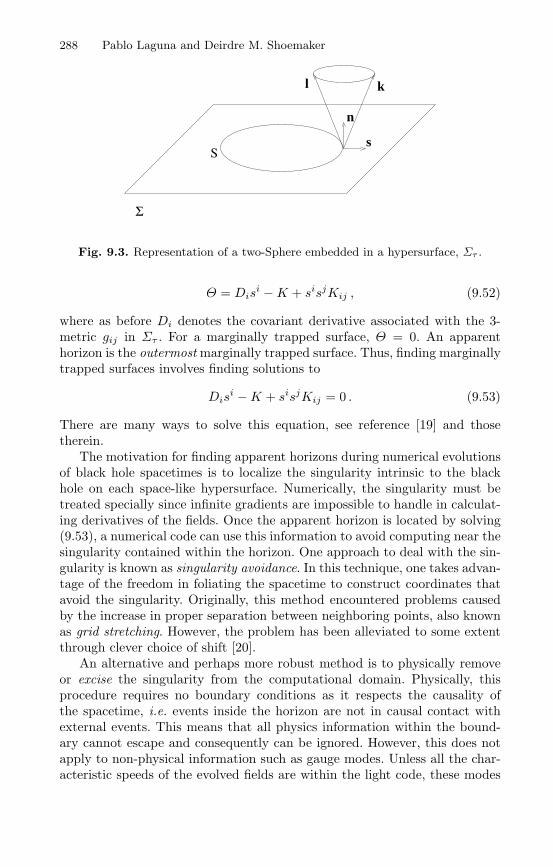
288 Pablo Laguna and Deirdre M. Shoemaker
Σ
s
kl
n
S
Fig. 9.3. Representation of a two-Sphere embedded in a hypersurface, Στ .
Θ = Disi −K + sisjKij , (9.52)
where as before Di denotes the covariant derivative associated with the 3-metric gij in Στ . For a marginally trapped surface, Θ = 0. An apparenthorizon is the outermost marginally trapped surface. Thus, finding marginallytrapped surfaces involves finding solutions to
Disi −K + sisjKij = 0 . (9.53)
There are many ways to solve this equation, see reference [19] and thosetherein.
The motivation for finding apparent horizons during numerical evolutionsof black hole spacetimes is to localize the singularity intrinsic to the blackhole on each space-like hypersurface. Numerically, the singularity must betreated specially since infinite gradients are impossible to handle in calculat-ing derivatives of the fields. Once the apparent horizon is located by solving(9.53), a numerical code can use this information to avoid computing near thesingularity contained within the horizon. One approach to deal with the sin-gularity is known as singularity avoidance. In this technique, one takes advan-tage of the freedom in foliating the spacetime to construct coordinates thatavoid the singularity. Originally, this method encountered problems causedby the increase in proper separation between neighboring points, also knownas grid stretching. However, the problem has been alleviated to some extentthrough clever choice of shift [20].
An alternative and perhaps more robust method is to physically removeor excise the singularity from the computational domain. Physically, thisprocedure requires no boundary conditions as it respects the causality ofthe spacetime, i.e. events inside the horizon are not in causal contact withexternal events. This means that all physics information within the bound-ary cannot escape and consequently can be ignored. However, this does notapply to non-physical information such as gauge modes. Unless all the char-acteristic speeds of the evolved fields are within the light code, these modes
9 Computational Black Hole Dynamics 289
can propagate out and affect the numerical stability. Excision has been im-plemented in many different formulations [21, 22, 23, 24, 25, 26, 27]. With therecent work on formulations, excision algorithms have been stably coded inhyperbolic and BSSN-type codes in stationary and dynamic back hole sys-tems [28, 29, 30, 31, 32].
Invariant physical information contained in the source simulations mustbe both extracted and interpreted if we are to construct a complete picture ofgravitational physics in the strong field regime. This is a daunting challengein general relativity where there is freedom in the choice of gauge and theform of the equations.
Of particular interest is the quantification of the mass M and angularmomentum J of a black hole. One way to attribute a mass and an angularmomentum to a black hole is to calculate the corresponding ADM quantitiesat infinity. The main difficulty is that the ADM mass and angular momentumrefer to the whole spacetime. In a dynamical situation, such a spacetime willcontain gravitational radiation and it is not clear how much of the mass orangular momentum should be attributed to the black hole itself and, if thereis more than one black hole, to each individual black hole. It is desirable tohave a framework that combines the properties of apparent horizons withthe powerful tools available at infinity. In the regime when the black hole isisolated in an otherwise dynamical spacetime, such a framework now existsin the form of isolated horizons [33, 34]. Isolated horizons provide a way toidentify a black hole quasi-locally and allow for the calculation of M andJ . It has been shown recently that the formula for angular momentum andmass arising from the isolated horizon formalism are valid even in dynamicalsituations [35, 36].
The theory of dynamical and isolated horizons gives rise to definitions forM and J that are similar in form to the ADM definitions, but are calculatedat the dynamical horizon ∆:
J∆ =18π
∮
S
(ϕasbKab) d2V , (9.54)
where Kab is the extrinsic curvature on S and ϕa is a Killing vector relatedto the fact that S must by axisymmetric in order for angular momentum tobe defined. In [37] a method for calculating ϕa based on the Killing transportequation is detailed.
Given J∆, the horizon mass M∆ is obtained from [38, 39]
M∆ =1
2R∆
√R4
∆ + 4J2∆ , (9.55)
where R∆ is the area radius of the horizon: R∆ = (A∆/4π)1/2. This formuladepends on R∆ and J∆ in the same way as in the Kerr solution. However,this is a result of the calculation and not an assumption. Furthermore, undersome physically reasonable assumptions on fields near future time-like infinity
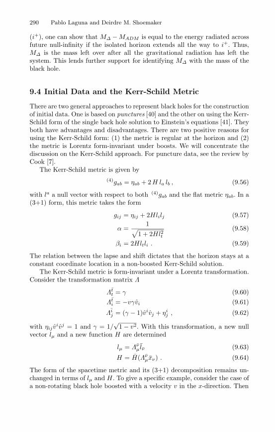
290 Pablo Laguna and Deirdre M. Shoemaker
(i+), one can show that M∆ −MADM is equal to the energy radiated acrossfuture null-infinity if the isolated horizon extends all the way to i+. Thus,M∆ is the mass left over after all the gravitational radiation has left thesystem. This lends further support for identifying M∆ with the mass of theblack hole.
9.4 Initial Data and the Kerr-Schild Metric
There are two general approaches to represent black holes for the constructionof initial data. One is based on punctures [40] and the other on using the Kerr-Schild form of the single back hole solution to Einstein’s equations [41]. Theyboth have advantages and disadvantages. There are two positive reasons forusing the Kerr-Schild form: (1) the metric is regular at the horizon and (2)the metric is Lorentz form-invariant under boosts. We will concentrate thediscussion on the Kerr-Schild approach. For puncture data, see the review byCook [7].
The Kerr-Schild metric is given by(4)gab = ηab + 2H la lb , (9.56)
with la a null vector with respect to both (4)gab and the flat metric ηab. In a(3+1) form, this metric takes the form
gij = ηij + 2Hlilj (9.57)
α =1
√1 + 2Hl2t
(9.58)
βi = 2Hltli . (9.59)
The relation between the lapse and shift dictates that the horizon stays at aconstant coordinate location in a non-boosted Kerr-Schild solution.
The Kerr-Schild metric is form-invariant under a Lorentz transformation.Consider the transformation matrix Λ
Λtt = γ (9.60)Λt
i = −vγvi (9.61)
Λij = (γ − 1)vivj + ηi
j , (9.62)
with ηij vivj = 1 and γ = 1/
√1 − v2. With this transformation, a new null
vector lµ and a new function H are determined
lµ = Λνµ lν (9.63)
H = H(Λνµxν) . (9.64)
The form of the spacetime metric and its (3+1) decomposition remains un-changed in terms of lµ and H. To give a specific example, consider the case ofa non-rotating black hole boosted with a velocity v in the x-direction. Then
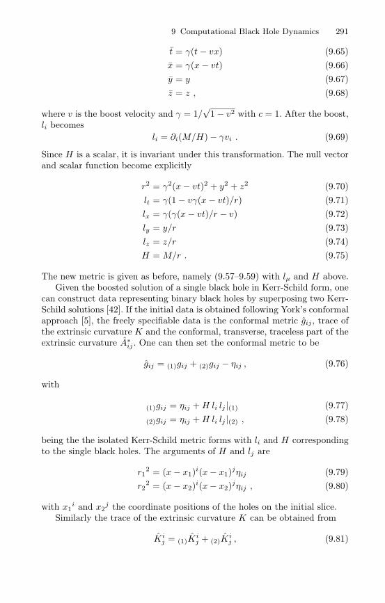
9 Computational Black Hole Dynamics 291
t = γ(t− vx) (9.65)x = γ(x− vt) (9.66)y = y (9.67)z = z , (9.68)
where v is the boost velocity and γ = 1/√
1 − v2 with c = 1. After the boost,li becomes
li = ∂i(M/H) − γvi . (9.69)
Since H is a scalar, it is invariant under this transformation. The null vectorand scalar function become explicitly
r2 = γ2(x− vt)2 + y2 + z2 (9.70)lt = γ(1 − vγ(x− vt)/r) (9.71)lx = γ(γ(x− vt)/r − v) (9.72)ly = y/r (9.73)lz = z/r (9.74)H = M/r . (9.75)
The new metric is given as before, namely (9.57–9.59) with lµ and H above.Given the boosted solution of a single black hole in Kerr-Schild form, one
can construct data representing binary black holes by superposing two Kerr-Schild solutions [42]. If the initial data is obtained following York’s conformalapproach [5], the freely specifiable data is the conformal metric gij , trace ofthe extrinsic curvature K and the conformal, transverse, traceless part of theextrinsic curvature A∗
ij . One can then set the conformal metric to be
gij = (1)gij + (2)gij − ηij , (9.76)
with
(1)gij = ηij +H li lj |(1) (9.77)
(2)gij = ηij +H li lj |(2) , (9.78)
being the the isolated Kerr-Schild metric forms with li and H correspondingto the single black holes. The arguments of H and lj are
r12 = (x− x1)i(x− x1)jηij (9.79)
r22 = (x− x2)i(x− x2)jηij , (9.80)
with x1i and x2
j the coordinate positions of the holes on the initial slice.Similarly the trace of the extrinsic curvature K can be obtained from
Kij = (1)K
ij + (2)K
ij , (9.81)

292 Pablo Laguna and Deirdre M. Shoemaker
where (1)Kij and (2)K
ij are the individual extrinsic curvatures associated with
the individual Kerr-Schild metrics. That is, one sets K = K(1)+K(2). Givengij and K, one is in the position to apply York’s conformal approach.
While both the puncture and superposed Kerr-Schild methods have beenused to generate initial data for binary black hole evolutions, it is important tonote that posing astrophysically relevant initial data in numerical relativityis very much an open question. Correct initial data would be supplied byPost-Newtonian calculations with numerical evolutions taking over wherethe Post-Newtonian approximations break down. This is not yet possiblewith current codes and computer technology. For this reason, it is importantto develop physical insight about how much spurious radiation is present inthe initial data. Some preliminary work in this area has been done [43].
9.5 Black Hole Evolutions
The first milestone to be achieved for the successful orbit and merger of twoblack holes is the stable, long term evolution of a single, static black hole.Despite the fact that the solution for a charge free single black hole is knownto be either Schwarzschild or Kerr, the numerical relativity community hasbeen struggling to obtain a generic, three-dimensional stable evolution foryears. Early on in the effort, two types of evolutions were pursued, those usingthe standard ADM formulation [44, 21, 22] and those using the characteristicformulation [45, 23]. Characteristic formulations achieved astounding successat evolving single black holes for arbitrary amounts of time while the (3+1)suffered severe stability problems when applied in three spatial dimensions.
Over the last several years, the community has come to understand thatthe problems were not solely numerical but originated in part from the struc-ture of the equations. The result is that (3+1) codes can now evolve singleblack holes stably in three dimensions. With a code based on the KST hy-perbolic formulation, the Cornell/Caltech group has been able to achieveevolution of a single black hole for (600 − 8000)M depending on the coordi-nates chosen [17]. Here constraint violations were tracked and determined tobe the possible culprit in the failure to evolve a single black hole in (3+1) forso many years. Similarly, several groups with codes based on the BSSN formof equations carried out black hole evolutions for hundreds to thousands ofM [46, 47, 31]. A crucial aspect in these simulations has the use of dynamical(driver) gauge conditions, as well as a densitized lapse [31].
In order to successfully compute the last few orbits and merger of twoblack holes, it is highly likely that one would have to develop a code capa-ble of moving excised black holes through the computational domain. Whilemuch of the current effort on orbits and head-on collisions has been accom-plished by holding the black holes fixed to the grid, it is our believe thatadding the flexibility for black holes to move or drift will greatly facilitatecoalescence simulations. This implies the development of excision algorithms

9 Computational Black Hole Dynamics 293
that populate points on the numerical grid with field values where there werenone at the previous time step [30].
Characteristic formulations had early success at moving black holesthrough the grid [23]. Although there was an early attempt at moving blackholes in (3+1) formulations [21], success depended on recent improvementsto the formulation of the (3+1) equations that has allowed the stable evo-lution of a stationary black hole. As a test of moving excision, evolutions ofa scalar field in a static or boosted Kerr-Schild black hole background [29]have been accomplished. Further, in [30, 31], full three-dimension evolutionswere performed of a single black hole in a coordinates systems in which thecoordinate location of the black hole did not remained fixed.
A truly dynamical test of codes designed to evolve black holes is the evo-lution of distorted black hole spacetimes. Distorted black holes are dynamicalsystems demanding many of the same technical and analytic developmentsthat binary black hole systems do. In addition there are interesting physicsregarding gravitational radiation and the dynamics of horizons that can beinvestigated with these systems. Many three dimensional simulations of dis-torted black holes have been carried out [48, 46, 49, 50, 51]. Typically, theblack hole is distorted by a wave, often a Brill wave [52]. The simulationswere primarily intended at testing gravitational wave extraction techniquesand the stability properties of the codes. Recently, distorted black holes [46]were used to test gauge conditions. These results showed a match to thelowest two quasi normal mode frequencies.
Highly distorted black holes provide a mechanism for a detailed charac-terization of the transition from a highly, nonlinear distorted black hole to aringing black hole and to the onset of quasi normal mode frequencies. Allenand collaborators [51] probed the nonlinear generation of harmonics for smallamplitudes of the ingoing wave. More recently, Papadopoulos [53] and Zlo-chower and his collaborators [54] have evolved distorted black holes using theCharacteristic framework. Both report interesting nonlinear effects such asmode mixing, larger phase shifts and amplitudes that may lend insight intothe observations of gravitational waves.
The effort on simulating head-on collisions provides a good picture ofthe early history of vacuum numerical relativity. The first attempt to solvethis problem took place as early as 1964 [55]. This and subsequent efforts onhead-on collision were carried out in axisymmetry, namely as a (2+1) problem[56, 25]. It was not until the late 90’s that computer speed and memory wassuch that 3D simulations were possible [20].
Despite the early difficulties in evolving single black holes stably, somegroups were capable of carrying out evolutions of black hole grazing collisions.Grazing collisions refer to collisions of slightly off-center head-on black holecollisions. The initial separation of the black holes was limited by the onsetof instabilities. Separation of the black holes were such that a joint apparenthorizon formed early in the simulation. These tests, however, demonstratedthe ability to do non-axisymmetric dynamic binary black hole simulations.
294 Pablo Laguna and Deirdre M. Shoemaker
Grazing collisions continue to be a step toward the orbit and merger of twoblack holes. Brugmann [57] completed the first grazing collision using theBrandt and Brugmann puncture method [40] to avoid the singularities duringthe computation. Although this evolution ended too prematurely to be ofastrophysical interest, it was the first three-dimensional binary black holeevolution. The first attempt to use dynamic singularity excision in grazingcollisions was carried out by the Penn State/Pittsburgh/Texas collaboration[22] using a code based on the standard ADM formulation. The initial datafor these simulations was the superposed Kerr-Schild data [42, 58]. Thesesimulations were successful in demonstrating the use of dynamic excision tofollow two back holes as they merge; however, the results were too short-livedand affected by boundary effects to allow for gravitational wave extraction.Soon after, a second grazing collision was completed by the AEI group atGermany [59]. This grazing collision did not used excision but puncturesto handle the black hole singularities. A combination of large amount ofsupercomputing power and coordinates to push outer boundaries sufficientlyfar allowed wave extraction to be obtained in these simulations.
Given the limitations of performing long-lived binary evolutions, theLazarus group [60] developed a framework to extend the life of the simula-tions by connecting at the end of fully nonlinear calculations a perturbativecalculation. Using an ADM code, the Lazarus effort was successful in con-structing waveforms from head-on [61] and merger from ISCO [62]. Whatappears to be the first fully nonlinear evolution of an orbit of two black holeswas performed only recently [63]. The simulation uses corotating coordinatesand dynamical shift conditions that force the black holes to stay fixed on thegrid. The simulation lasts about one orbital period before crashing. Whilethis works does not yet provide detailed waveforms useful to data analysiseffort, they however demonstrate the advances made over the last few years.
9.6 Conclusions and Future Work
Over the last decade or more, the numerical relativity community has focusedmost of its attention to the binary black hole problem. Although early effortswere seriously plagued by numerical instabilities, simulations in which theseinstabilities are been tamed is gaining momentum. There are still many openproblems before simulations of orbits and mergers, such as the ones reportedabove, can be enhanced to the point in which useful astrophysical predictionsare possible. One of the major obstacles is specifying the astrophysically rele-vant initial data; this requires a framework for incorporating post-Newtonianinformation into numerical source simulations. A second obstacle is accuratewave extraction, namely the translation of numerically evolved quantities intophysical invariants. In addition, we are lacking good outer boundary condi-tions although it is encouraging to see that there has been work toward thedesign of constraint-preserving boundary conditions. There are more difficul-
9 Computational Black Hole Dynamics 295
ties ahead, but the difference between today and five years ago is that todaythe challenges are met with codes that can successfully evolve single blackhole, as well as modest binary black hole evolutions.
Of great significance has been the progress made in formulating the (3+1)decomposition of the Einstein equation and dynamical gauge conditions.With the advent of adaptive mesh refinements (AMR), the outlook for nu-merical relativity is positive and fast paced. AMR is essential if one has anyhope of simulating astrophysical black hole orbits. Currently the effort hasbeen focused on fixed mesh refinement [63, 64, 65]. Adaptivity can be alsoachieved by other means beside AMR. For instance, the groups at Meudonand Caltech/Cornell have pioneered the use of pseudo-spectral methods hav-ing this in mind [66, 67, 68]. Preliminary work is currently taking place also onthe use of finite element techniques, a method with a high degree of intrinsicadaptivity.
The detection of gravitational radiation will supply us with means toprobe the fundamental nature of gravity. The information obtained fromsource simulations will have a profound impact to the data analysis commu-nity now searching for evidence of gravitational waves in the ground-baseddetector’s data stream. With the possibility of high quality source simula-tions, the community must begin to interface with data analysis. While it islikely that the outcome from numerical simulations to be handed to the dataanalysis community will not be an exhaustive collection of waveforms, sourcesimulations could nonetheless provide robust information (e.g. frequency evo-lutions, mode content, etc.) of extremely high value to the observational ef-fort.
Acknowledgments
This work was supported by NSF grants PHY-9900672 and PHY-0312072at Cornell and PHY-9800973 and PHY-0114375 at Penn State. Work sup-ported in part by the Center for Gravitational Wave Physics funded by theNational Science Foundation under Cooperative Agreement PHY-0114375.The authors would like to thank the organizers of this conference for the op-portunity to be part of the Second Aegean school and to visit such a beautifulplace as Syros.
References
1. M. Maggiore, Gravitational Wave Experiments and Early Universe Cosmology,Phys. Reports, 331, 283 (2000).
2. T.W. Baumgarte and S.L. Shapiro. Numerical relativity and compact binaries.Phys. Reports, 376, 41 2003.
3. C. Cluter and K.S. Thorne. An overview of gravitational-wave sources. InProceeding of GR16, 2001.
296 Pablo Laguna and Deirdre M. Shoemaker
4. L. Lehner, Numerical relativity: A review, Class. Quant. Grav. 18, R25 (2001).5. J. W. York Jr, Kinematics and dynamics of general relativity, In L. L. Smarr,
editor, Sources of gravitational radiation, pages 83–126. Cambridge UniversityPress, Cambridge, (1979).
6. R. Arnowitt, S. Deser, and C.W. Misner, The dynamics of general relativity,In L. Witten, editor, Gravitation an introduction to current research, pages227–265. John Wiley, New York, (1962).
7. G.B. Cook, Living Rev. Rel. 5, 1 (2000).8. G. Calabrese and O. Sarbach, J. Math. Phys. 44, 3888 (2003).9. M. Alcubierre, Class. Quant. Grav. 20, 607 (2003).
10. M. Tiglio, L. Lehner, and D. Nilsen, gr-qc/0312001 (2003).11. L. Lindblom, M. A. Scheel, L. E. Kidder, H. P. Pfeiffer, D. Shoemaker, and
S. A. Teukolsky, gr-qc/0402027, (2004).12. M. Anderson amd R.A. Matzner, gr-qc/0307055 (2003).13. H. Shinkai and G. Yoneda, gr-qc/0209111, (2002).14. O. Reula, Living Rev. Rel. 3, 1 (1998).15. T.W. Baumgarte and S.L. Shapiro, Phys. Rev. D 59, 024007 (1999).16. M. Shibata and T. Nakamura, Phys. Rev. D 52, 5428 (1995).17. L.E. Kidder, M.A. Scheel, and S.A. Teukolsky, Extending the lifetime of 3d
black hole computations with a new hyperbolic system of evolution equations,Phys. Rev. D64, 064017 (2001).
18. J. York, In C.R. Evans and L.S. Finn and D.W. Hobill, editors, Frontiers inNumerical Relativity, Cambridge University Press, Cambridge, (1989).
19. J. Thornburg, A fast apparent-horizon finder for 3-dimensional cartesian gridsin numerical relativity, Class. Quant. Grav. 21, 743 (2004).
20. M. Alcubierre, B. Brugmann, P. Diener, M. Koppitz, D. Pollney, E. Seidel, andR. Takahashi, Gauge conditions for long-term numerical black hole evolutionswithout excision, Phys. Rev. D67, 084023 (2003).
21. G.B. Cook and BBH Alliance, Boosted three-dimensional black hole evolutionswith singularity excision, Phys. Rev. Lett. 80, 2512 (1998).
22. S. Brandt, R. Correll, R. Gomez, M. Huq, P. Laguna L. Lehner, D. Neilsen,R. Matzner, J. Pullin, E. Schnetter, D. Shoemaker, and J. Winicour, Grazingcollisions of black holes via the excision of singularities, Phys. Rev. Lett. 85,5496 (2000).
23. R. Gomez, L. Lehner, R. Marsa, and J. Winicour, Moving black holes in 3d,Phys. Rev. D57, 4778 (1998).
24. E. Seidel and W. Suen, Phys. Rev. Lett. 69, 1845 (1992).25. P. Anninos, G. Gaues, J. Masso, E. Seidel, and L. Smarr, Horizon boundary
condition for black hole spacetimes, Phys. Rev. D51, 5562 (1995).26. R. Marsa and M. Choptuik, Black hole–scalar field interactions in spherical
symmetry, Phys. Rev. D54, 4929 (1996).27. M. Scheel, T. Baumgarte, G. Cook, S. Shapiro, and S. Teukolsky, Numerical
evolution of black holes with a hyperbolic formulation of general relativity,Phys. Rev. D56, 6320 (1997).
28. M. Alcubierre and B. Brugmann, Simple excision of a black hole in 3+1 nu-merical relativity, Phys. Rev. D63, 104006 (2001).
29. H. Yo, T. Baumgarte, and S. Shapiro, A numerical testbed for singularityexcision in moving black hole spacetimes, Phys. Rev. D64, 124011 (2001).
30. D. Shoemaker, K. Smith, U. Sperhake, P. Laguna, E. Schnetter, and D. Fiske,Class. Quant. Grav. 20, 3729 (2003).
9 Computational Black Hole Dynamics 297
31. U. Sperhake, K. Smith, B. Kelly, P. Laguna, and D. Shoemaker, Phys. Rev.D69, 024012 (2004).
32. G. Calabrese, L. Lehner, D. Neilsen, J. Pullin, O. Reula, O. Sarbach, andM. Tiglio, Novel finite-differencing techniques for numerical relativity: appli-cation to black hole excision, Class. Quant. Grav. 20, L245 (2003).
33. A. Ashtekar, C. Beetle, and S. Fairhurst, Mechanics of isolated horizons, Class.Quant. Grav. 17, 253 (2000).
34. A. Ashtekar, C. Beetle, O. Dreyer, S. Fairhurst, B. Krishnan, J. Lewandowski,and J. Wisniewski, Generic isolated horizons and their applications, Phys. Rev.Lett. 85, 3564 (2000).
35. A. Ashtekar and B. Krishnan, Dynamical horizons: Energy, angular momentum,fluxes and balance laws, Phys. Rev. Lett. 89, 261101 (2002).
36. A. Ashtekar and B. Krishnan, Dynamical horizons and their properties, Phys.Rev. D68, 104030 (2003).
37. O. Dreyer, B. Krishnan, E. Schnetter, and D. Shoemaker, Introduction toisolated horizons in numerical relativity, Phys. Rev. D67, 024018 (2003).
38. A. Ashtekar, S. Fairhurst, and B. Krishnan, Isolated horizons: Hamiltonianevolution and the first law, Phys. Rev. D62, 104025 (2000).
39. A. Ashtekar, C. Beetle, and J. Lewandowski, Mechanics of rotating isolatedhorizons, Phys. Rev. D64, 044016 (2001).
40. S. Brandt and B. Brugmann, A simple construction of initial data for multipleblack holes, Phys. Rev. Lett. 78, 3606 (1997).
41. C.W. Misner, K.S. Thorne, and J.A. Wheeler, Gravitation. Freeman: SanFrancisco, (1973).
42. R.A. Matzner, M.F. Huq, and D. Shoemaker, Initial data and coordinates formultiple black hole systems, Phys. Rev. D59, 024015 (1999).
43. Harald P. Pfeiffer and Gregory B. Cook and Saul A. Teukolsky, Comparinginitial-data sets for binary black holes, Phys. Rev. D66, 024047 (2002).
44. P. Anninos, K. Camarda J. Masso, E. Seidel, W. Suen, and J. Towns, Threedimensional numerical relativity: the evolution of black holes, Phys. Rev. D52,2059 (1995).
45. R. Gomez et al, Stable characteristic evolution of generic three-dimensionalsingle black hole space-times, Phys. Rev. Lett. 80, 3915 (1998).
46. M. Alcubierre, B. Brugmann, D. Pollney, E. Seidel, and R. Takahashi, Blackhole excision for dynamic black holes, Phys. Rev. D64, 061501 2001.
47. H.-J. Yo, T. W. Baumgarte, and S. L. Shapiro, Phys. Rev. D66, 084026 (2002).48. S. Brandt, K. Camarda, E. Seidel, and R. Takahashi, Three dimensional dis-
torted black holes, Class. Quant. Grav. 20, 1 (2003).49. R. Gomez, Gravitational waveforms with controlled accuracy, Phys. Rev. D64,
024007 (2001).50. J. Baker, S. Brandt, M. Campanelli, C. Lousto, E. Seidel, and R. Takahashi,
Nonlinear and perturbative evolution of distorted black holes. ii. odd-paritymodes, Phys. Rev. D62, 127701 (2000).
51. G. Allen, K. Camarda, and E. Seidel, Black hole spectroscopy: Determiningwaveforms from 3d excited black holes, gr-qc/9806036 (1998).
52. D.R. Briland and R.W. Lindquist, Phys. Rev. 131, 471 (1963).53. P. Papadopoulos, Nonlinear harmonic generation in finite amplitude black hole
oscillations, Phys. Rev. D65, 084016 2002.54. Y. Zlochower, R Gomez, S. Husa, L. Lehner, and J. Winicour, Mode coupling
in the nonlinear response of black holes, Phys. Rev. D68, 084014 (2003).
298 Pablo Laguna and Deirdre M. Shoemaker
55. S. Hahn and R. Lindquist, The two body problem in geometrodynamics, Annalsof Physics 29, 304 (1964).
56. L. L. Smarr, Gauge conditions, radiation formulae and the two black holecollisions, In L. L. Smarr, editor, Sources of gravitational radiation, page 275.Cambridge University Press, Cambridge, (1979).
57. B. Brugmann, Binary black hole mergers in 3d numerical relativity, Int. J.Mod. Phys. D8, 85 (1999).
58. P. Marronetti, M. Huq, P. Laguna, L. Lehner, R. Matzner, and D. Shoemaker,Approximate analytical solutions to the initial data problem of black hole bi-nary systems, Phys. Rev. D62, 024017 (2000).
59. M. Alcubierre, W. Benger, B. Brugmann, G. Lanfermann, L. Nerger, E. Seidel,and R. Takahashi, The 3d grazing collision of two black holes, Phys. Rev. Lett.87, 271103 (2001).
60. J. Baker, M. Campanelli, C.O. Lousto, and R. Takahashi, The lazarus project:A pragmatic approach to binary black hole evolutions, Phys. Rev. D 65, 124012(2002).
61. J. Baker, B. Brugmann, M. Campanelli, and C.O. Lousto, Gravitational wavesfrom black hole collisions via an eclectic approach, Class. Quant. Grav. 17,L149 (2000).
62. J. Baker, , B. Brugmann, M. Campanelli, C.O. Lousto, and R. Takahashi,Plunge waveforms from inspiralling binary black holes, Phys. Rev. Lett. 87,121103 (2001).
63. B. Brugmann, W. Tichy, and N. Jansen, Numerical simulation of orbiting blackholes, gr-qc/0312112 (2003).
64. E. Schnetter, S. Hawley, and I. Hawke, Evolutions in 3d numerical relativityusing fixed mesh refinement, Class. Quant. Grav 21, 1465 (2004).
65. B. Imbiriba, J. Baker, D. Choi, J. Centrella, D. Fiske, J. Brown, J. van Meter,and K. Olson, Evolving a puncture black hole with fixed mesh refinement,gr-qc/0403048 (2004).
66. L. Kidder, M. Scheel, S. Teukolsky, E. Carlson, and G. Cook, Black holeevolution by spectral methods, Phys. Rev. D62, 084032 (2000).
67. S. Bonazzola, E. Gourgoulhon, and J. Marck, Spectral methods in generalrelativistic astrophysics, J. Comput. Appl. Math. 109, 892 (1999).
68. P. Grandclement, S. Bonazzola, E. Gourgoulhon, and J. Marck, A multi-domainspectral method for scalar and vectorial poisson equations with non-compactsources, J. Comput. Phys. 170, 231 (2001).

Index
Accelerating Universe 155Acoustic Peaks 57, 79, 83, 122Adiabatic Fluctuations 82Adiabatic Perturbations 47ADM formulation 282ADM Mass 289Age of the Universe 119Angular Size Test 121Apparent Horizon 287Asteroseismology 273
Bardeen Potential 38, 65Baryon Asymmetry 27Binary Systems 266Branes 185Braneworld Cosmology 227Braneworld Inflation 230Braneworld Perturbations 64, 234
Calabi-Yau Spaces 193Chaotic Inflation 26Chaplygin Gas 164Coincidence Puzzle 22Cold Dark Matter 144, 145Color Index 108Comoving Coordinate System 4Compactification 187Continuity Equation 10Cosmic Microwave Background 7, 112Cosmic Microwave Background
Anisotropies 55, 73Cosmic Microwave Background
Polarization 94
Dark Energy 17, 92, 110, 150Dark Matter 17, 141Dark Radiation 224de Sitter Space 11
Deceleration Parameter 5, 154Dp-Branes 186, 214Duality 199
Early Universe Gravitational Waves274
Event Horizon 287
f-Modes 270Flatness Problem 23Flux-Redshift Test 125Friedmann Models 8
Gauss-Codazzi Equations 220Geometrodynamics 279Graceful Exit 203Gravitational Collapse 266Gravitational Lenses 119, 149Gravitational Wave Perturbations
239
Harmonic Decomposition 35Harrison-Zel’dovich Spectrum 51, 61Heterotic M-Theory 192High-Frequency Gravitational Waves
265Horizon Problem 20Hot Dark Matter 144Hubble Law 3, 9Hubble Parameter 10, 154
Induced Gravity Model 134, 162Inflation 25Isocurvature Fluctuations 84
Kahler Metric 191Kahler Potential 190Kaluza-Klein Modes 222Kerr-Schild Metric 290
300 Index
Lapse Function 280Luminosity Distance 155
M-Theory 181, 213M-Theory and Inflation 200Malmquist Effect 129Matter Dominated Universe 13Metric Perturbations 37Modified Newtonian Dynamics 149Moduli Fields 190Moving Branes 198
New Inflation 26Number Counts of Faint Galaxies
129
Old Inflation 26
Perturbations During Inflation 51Phantom Energy 165Photon-Baryon Dynamics 79Power Spectrum 58, 92Pre-Big-Bang Inflation 202
Quadrupole Formula 262Quadrupole Moment 263Quasi-normal Modes 267Quintessence 110, 158
Quintessential Inflation 162
r-Modes 270Radiation Dominated Universe 12Randall-Sundrum Model 161, 216Reionization 87Robertson-Walker Metric 8Rotational Instabilities 268
Sachs-Wolfe Effect 57, 87, 237Scalar Perturbations 51Schwarzschild-AdS5 Metric 228Singularity 288Spectral Index 99Sunyaev-Zeldovich Effect 118Supergravity Theories 189
Temperature Anisotropies 74Tensor Perturbations 54Topology Change in Cosmology 204Trapped Surfaces 287Tully-Fisher Relation 118
Vacuum Energy 11Vacuum Energy and the Cosmological
Constant 150Vector Perturbations 53Velocity-Distance Law 3