Embed Size (px)
Citation preview
INSTITUTE OF PHYSICS PUBLISHING REPORTS ON PROGRESS IN PHYSICS
Rep. Prog. Phys. 67 (2004) 1429–1496 PII: S0034-4885(04)25227-7
The physics of earthquakes
Hiroo Kanamori1 and Emily E Brodsky2
1 Seismological Laboratory, California Institute of Technology, Pasadena, CA 91125, USA2 Department of Earth & Space Sciences, University of California, Los Angeles,Los Angeles, CA 90095, USA
Received 21 January 2004, in final form 20 April 2004Published 12 July 2004Online at stacks.iop.org/RoPP/67/1429doi:10.1088/0034-4885/67/8/R03
Abstract
Earthquakes occur as a result of global plate motion. However, this simple picture is far fromcomplete. Some plate boundaries glide past each other smoothly, while others are punctuatedby catastrophic failures. Some earthquakes stop after only a few hundred metres while otherscontinue rupturing for a thousand kilometres. Earthquakes are sometimes triggered by otherlarge earthquakes thousands of kilometres away. We address these questions by dissecting theobservable phenomena and separating out the quantifiable features for comparison acrossevents. We begin with a discussion of stress in the crust followed by an overview ofearthquake phenomenology, focusing on the parameters that are readily measured by currentseismic techniques. We briefly discuss how these parameters are related to the amplitudeand frequencies of the elastic waves measured by seismometers as well as direct geodeticmeasurements of the Earth’s deformation. We then review the major processes thought to beactive during the rupture and discuss their relation to the observable parameters. We then takea longer range view by discussing how earthquakes interact as a complex system. Finally, wecombine subjects to approach the key issue of earthquake initiation. This concluding discussionwill require using the processes introduced in the study of rupture as well as some novelmechanisms. As our observational database improves, our computational ability acceleratesand our laboratories become more refined, the next few decades promise to bring more insightson earthquakes and perhaps some answers.
(Some figures in this article are in colour only in the electronic version)
0034-4885/04/081429+68$90.00 © 2004 IOP Publishing Ltd Printed in the UK 1429
1430 H Kanamori and E E Brodsky
Contents
PageList of frequently used symbols 1432
1. Introduction 14332. Earthquakes and stress in the crust 1435
2.1. Plate motion and earthquake repeat times 14352.2. The state of stress in the crust 1436
Principal stresses and fault orientation 1438Strength of the crust: laboratory and field data 1439Conflicting observations? 1440Summary 1441
3. Quantifying earthquakes 14413.1. Earthquake source parameters and observables 1442
A formal description of the elastic problem 14423.1.1. Seismic source and displacement field 14433.1.2. Seismic moment and magnitude 14453.1.3. Strain and stress drop 14463.1.4. Energy 1447
Radiated energy, ER 1447Potential energy 1448
3.1.5. Rupture mode, speed and directivity 1449Directivity and source duration 1449Rupture speed 1449
3.1.6. Earthquake rupture pattern 14503.2. Seismic scaling relations 1451
3.2.1. Scaling relations for static parameters 14513.2.2. Scaling relations for dynamic parameters 1454
4. Rupture processes 14554.1. Fracture mechanics 1455
4.1.1. An overview of the crack model 14554.1.2. Crack tip breakdown-zone 14574.1.3. Stability and growth of a crack 1457
Static crack 1459Dynamic crack 1459Rupture speed 1459
4.2. Frictional sliding 14604.2.1. Static and kinetic friction 14614.2.2. Rate- and state-dependent friction 1461
4.3. The link between the crack model and the friction model 1463Direct determination of Dc 1463
4.4. Rupture energy budget 14634.5. Fault-zone processes: melting, fluid pressurization and lubrication 1466
Melting 1466
The physics of earthquakes 1431
Thermal fluid pressurization 1466Lubrication 1468
4.6. Linking processes to the seismic data 14684.6.1. The interpretation of macroscopic seismological parameters 1468
Radiation efficiency 1468The relation between radiation efficiency and rupture speed 1471Summary and implications 1471
5. Earthquakes as a complex system 1473The magnitude–frequency relationship
(the Gutenberg–Richter relation) 1473Simple models 1474
6. Instability and triggering 14766.1. Instability 1476
6.1.1. Stick slip and instability 1476Stiffness of the fault system 1478
6.1.2. Nucleation zone 14786.2. Triggering 1479
6.2.1. Observations 14796.2.2. Triggering with the rate- and state-dependent friction mechanism 1482
Spontaneous behaviour 1483Loading at a uniform rate 1483Stepwise change in loading 1483
6.2.3. Triggering with the stress corrosion mechanism 14846.2.4. Aftershocks and Omori’s Law 1486
State- and rate-dependent friction and Omori’s Law 1486Stress corrosion model and Omori’s Law 1488
6.2.5. Hydrologic barrier removal 14907. Conclusions 1491
Acknowledgments 1492References 1492

1432 H Kanamori and E E Brodsky
List of frequently used symbols
A constant in the rate- and state-friction lawa half-length of Mode III crackα P-wave speedB constant in the rate- and state-friction lawb slope of the earthquake magnitude–frequency relationshipβ S-wave speedχ probability of earthquake occurrenceD fault slip offsetD average offsetD0 critical slip of a crackDc critical displacement in the slip-weakening modelsδ slip on a frictional surfaceδ slip speedE elastic modulusER radiated seismic energyEG fracture energy of the earthquakeEH thermal energy (frictional energy loss) of the earthquakee scaled energy (the ratio of radiated seismic energy to seismic moment)G dynamic energy release rate (dynamic crack extension force)G∗ static energy release rate (static crack extension force, specific
fracture energy)G∗
c critical specific fracture energyγ surface energyη viscosity, seismic efficiencyηR radiation efficiencyK stress intensity factorKc fracture toughness (critical stress intensity factor)k stiffness of spring, permeabilitykf stiffness of the faultL length scale of the faultLn nucleation lengthl0 crack breakdown lengthM0 seismic momentMw earthquake magnitude (moment magnitude)µ rigidity (shear modulus) or coefficient of frictionµs coefficient of static frictionµk coefficient of kinetic frictionp pore pressure, power of the stress–corrosion relation, power of Omori’s LawQ heatR seismicity rater0 background seismicity rateρ densityS fault areaσ0 initial stress
The physics of earthquakes 1433
σ1 final stress (sections 3 to 6)σf frictional stressσs static stress drop (σ0 − σ1)
σij stress tensor(σ1, σ2, σ3) principal stresses (section 2)σY yield stressσn normal stressτ shear stress, source durationτ average source durationτ stress rateθ state variable in rate- and state-dependent friction; angle between the
fault and the maximum compressional stressui displacement vectorV rupture speedW0 initial (before an earthquake) potential energy of the EarthW1 final (after an earthquake) potential energy of the EarthW change in the potential energyW0 change in the potential energy minus frictional energyw width of the fault slip zone
1. Introduction
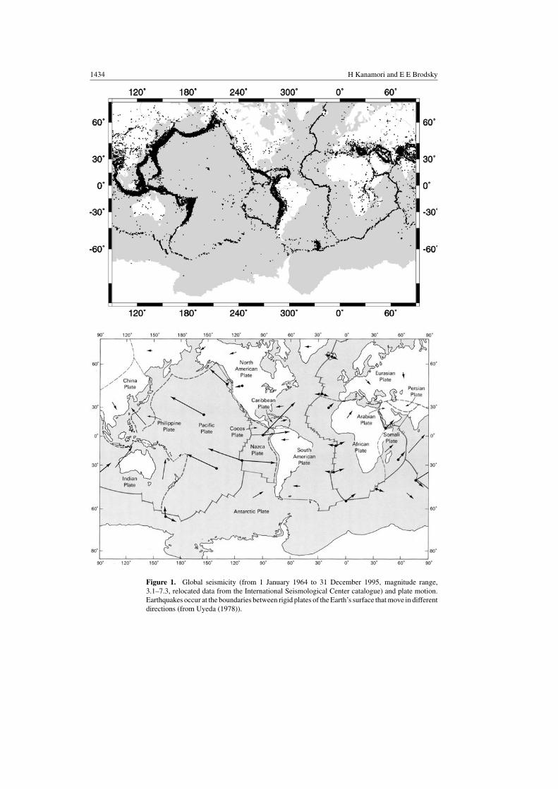
Why do earthquakes happen? This age-old question was solved at one level by the platetectonics revolution in the 1960s. Large, nearly rigid plates of the Earth slide past each other.Earthquakes accommodate the motion (figure 1). However, this simple answer is far fromcomplete. Some plate boundaries glide past each other smoothly, while others are punctuatedby catastrophic failures. Why is so little motion accommodated by anything in betweenthese two extremes? Why do some earthquakes stop after only a few hundred metres whileothers continue rupturing for a thousand kilometres? How do nearby earthquakes interact?Why are earthquakes sometimes triggered by other large earthquakes thousands of kilometresaway?
Earthquake physicists have attempted to answer these questions by dissecting observablephenomena and separating out the quantifiable features for comparison across events. Webegin this review with a discussion of stress in the crust followed by an overview ofearthquake phenomenology, focusing on the parameters that are readily measured by currentseismic techniques. We briefly discuss how these parameters are related to the amplitudeand frequencies of the elastic waves measured by seismometers as well as direct geodeticmeasurements of the Earth’s deformation. We then review the major processes thought to beactive during rupture and discuss their relationship to the observable parameters. We then takea longer range view by discussing how earthquakes interact as a complex system. Finally,we combine subjects to approach the key issue of earthquake initiation. This concludingdiscussion will require using the processes introduced in the study of rupture, as well as somenovel mechanisms.
In this introductory review for non-specialists, we gloss over many exciting and importantadvances in recent years ranging from the discovery of periodic slow slip events (Dragertet al 2001) to the elucidation of fault structure revealed by new accurate location techniques(Rubin et al 1999). Many of these recent advances are made possible by new technology
1434 H Kanamori and E E Brodsky
Figure 1. Global seismicity (from 1 January 1964 to 31 December 1995, magnitude range,3.1–7.3, relocated data from the International Seismological Center catalogue) and plate motion.Earthquakes occur at the boundaries between rigid plates of the Earth’s surface that move in differentdirections (from Uyeda (1978)).
The physics of earthquakes 1435
such as satellite geodesy and high-power computation. In order to interpret the newtechnological advances, we must return to and push the boundaries of classical mechanicaltheories. The approach we take here is to emphasize the features of classical theory thatare directly applicable to current, cutting-edge topics. Where possible, we highlight modernobservations and laboratory results that confirm, refute or extend elements of the classicalphysics-based paradigm. Inevitably, our examples tend to be biased towards our own interestsand research. We hope that this review will equip the reader to be properly sceptical of ourresults.
2. Earthquakes and stress in the crust
Earthquakes are a mechanism for accommodating large-scale motion of the Earth’s plates.As the plates slide past each other, relative motion is sometimes accommodated by a relativelyconstant gradual slip, at rates of the order of millimetres per year; while at other times, theaccumulated strain is released in earthquakes with slip rates of the order of metres per second.Sometimes, slip is accommodated by slow earthquakes or creep events with velocities of theorder of centimetre per month between the two extreme cases. Current estimates are that about80% of relative plate motion on continental boundaries is accommodated in rapid earthquakes(Bird and Kagan 2004). With few exceptions, earthquakes do not generally occur at regularintervals in time or space.
2.1. Plate motion and earthquake repeat times
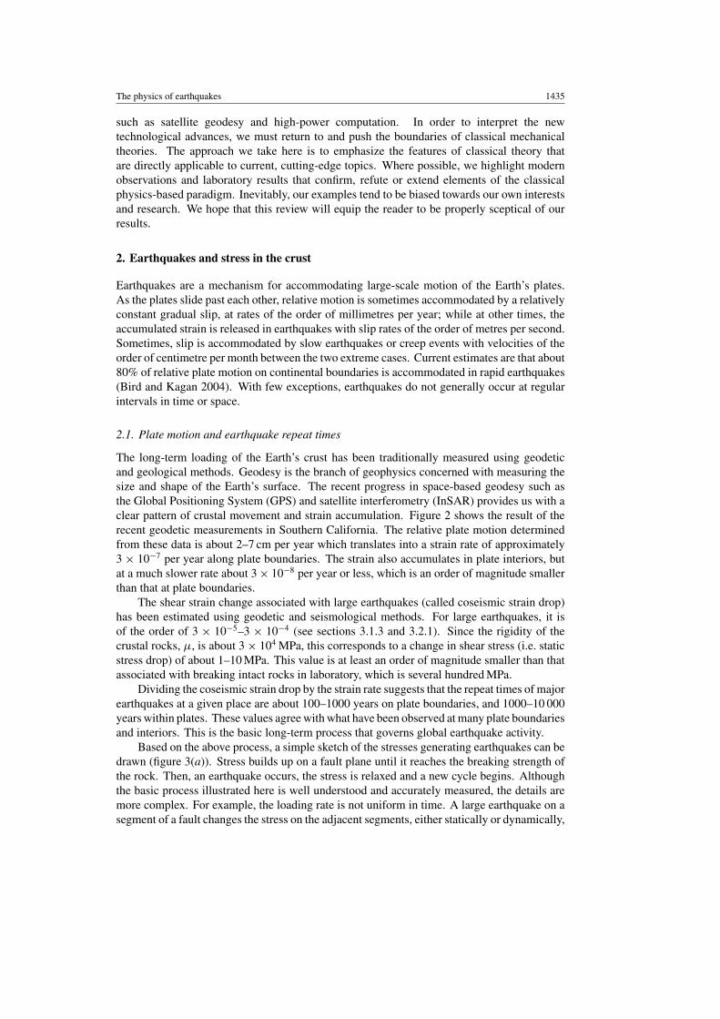
The long-term loading of the Earth’s crust has been traditionally measured using geodeticand geological methods. Geodesy is the branch of geophysics concerned with measuring thesize and shape of the Earth’s surface. The recent progress in space-based geodesy such asthe Global Positioning System (GPS) and satellite interferometry (InSAR) provides us with aclear pattern of crustal movement and strain accumulation. Figure 2 shows the result of therecent geodetic measurements in Southern California. The relative plate motion determinedfrom these data is about 2–7 cm per year which translates into a strain rate of approximately3 × 10−7 per year along plate boundaries. The strain also accumulates in plate interiors, butat a much slower rate about 3 × 10⁻⁸ per year or less, which is an order of magnitude smallerthan that at plate boundaries.
The shear strain change associated with large earthquakes (called coseismic strain drop)has been estimated using geodetic and seismological methods. For large earthquakes, it isof the order of 3 × 10⁻⁵–3 × 10⁻⁴ (see sections 3.1.3 and 3.2.1). Since the rigidity of thecrustal rocks, µ, is about 3 × 10⁴ MPa, this corresponds to a change in shear stress (i.e. staticstress drop) of about 1–10 MPa. This value is at least an order of magnitude smaller than thatassociated with breaking intact rocks in laboratory, which is several hundred MPa.
Dividing the coseismic strain drop by the strain rate suggests that the repeat times of majorearthquakes at a given place are about 100–1000 years on plate boundaries, and 1000–10 000years within plates. These values agree with what have been observed at many plate boundariesand interiors. This is the basic long-term process that governs global earthquake activity.
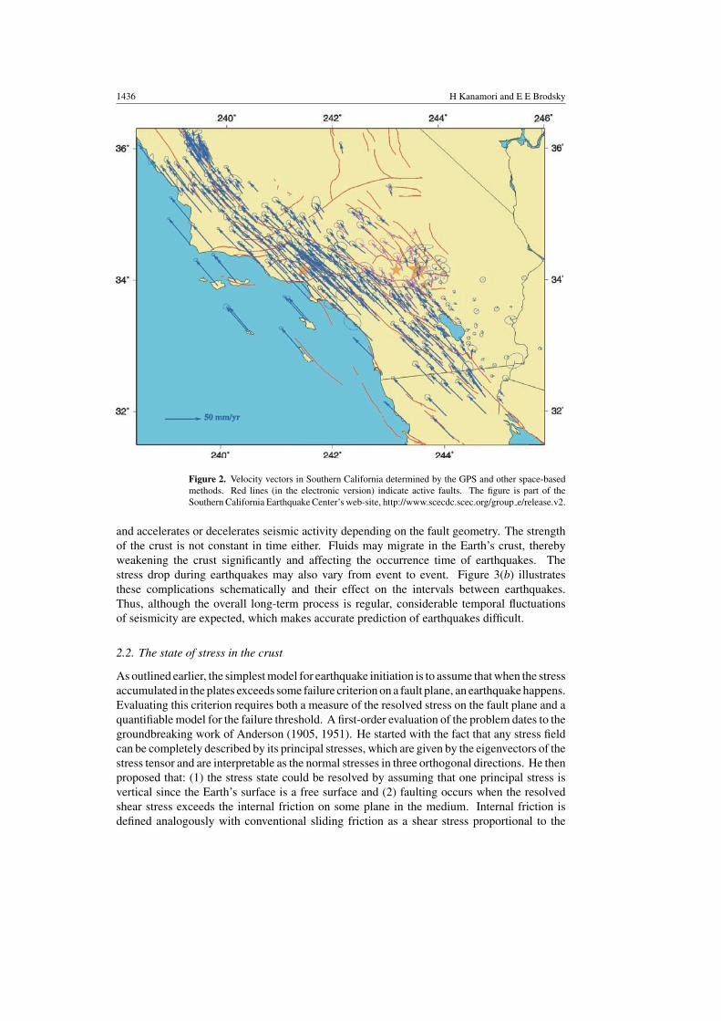
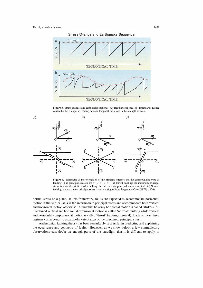
Based on the above process, a simple sketch of the stresses generating earthquakes can bedrawn (figure 3(a)). Stress builds up on a fault plane until it reaches the breaking strength ofthe rock. Then, an earthquake occurs, the stress is relaxed and a new cycle begins. Althoughthe basic process illustrated here is well understood and accurately measured, the details aremore complex. For example, the loading rate is not uniform in time. A large earthquake on asegment of a fault changes the stress on the adjacent segments, either statically or dynamically,
1436 H Kanamori and E E Brodsky
Figure 2. Velocity vectors in Southern California determined by the GPS and other space-basedmethods. Red lines (in the electronic version) indicate active faults. The figure is part of theSouthern California Earthquake Center’s web-site, http://www.scecdc.scec.org/group e/release.v2.
and accelerates or decelerates seismic activity depending on the fault geometry. The strengthof the crust is not constant in time either. Fluids may migrate in the Earth’s crust, therebyweakening the crust significantly and affecting the occurrence time of earthquakes. Thestress drop during earthquakes may also vary from event to event. Figure 3(b) illustratesthese complications schematically and their effect on the intervals between earthquakes.Thus, although the overall long-term process is regular, considerable temporal fluctuationsof seismicity are expected, which makes accurate prediction of earthquakes difficult.
2.2. The state of stress in the crust
As outlined earlier, the simplest model for earthquake initiation is to assume that when the stressaccumulated in the plates exceeds some failure criterion on a fault plane, an earthquake happens.Evaluating this criterion requires both a measure of the resolved stress on the fault plane and aquantifiable model for the failure threshold. A first-order evaluation of the problem dates to thegroundbreaking work of Anderson (1905, 1951). He started with the fact that any stress fieldcan be completely described by its principal stresses, which are given by the eigenvectors of thestress tensor and are interpretable as the normal stresses in three orthogonal directions. He thenproposed that: (1) the stress state could be resolved by assuming that one principal stress isvertical since the Earth’s surface is a free surface and (2) faulting occurs when the resolvedshear stress exceeds the internal friction on some plane in the medium. Internal friction isdefined analogously with conventional sliding friction as a shear stress proportional to the
The physics of earthquakes 1437
Figure 3. Stress changes and earthquake sequence. (a) Regular sequence. (b) Irregular sequencecaused by the changes in loading rate and temporal variations in the strength of crust.
(a) (b) (c)
Figure 4. Schematic of the orientation of the principal stresses and the corresponding type offaulting. The principal stresses are σ1 > σ2 > σ3. (a) Thrust faulting: the minimum principalstress is vertical. (b) Strike-slip faulting: the intermediate principal stress is vertical. (c) Normalfaulting: the maximum principal stress is vertical (figure from Jaeger and Cook (1979) p 426).
normal stress on a plane. In this framework, faults are expected to accommodate horizontalmotion if the vertical axis is the intermediate principal stress and accommodate both verticaland horizontal motion otherwise. A fault that has only horizontal motion is called ‘strike-slip’.Combined vertical and horizontal extensional motion is called ‘normal’ faulting while verticaland horizontal compressional motion is called ‘thrust’ faulting (figure 4). Each of these threeregimes corresponds to a particular orientation of the maximum principal stress.
Andersonian faulting theory has been remarkably successful in predicting and explainingthe occurrence and geometry of faults. However, as we show below, a few contradictoryobservations cast doubt on enough parts of the paradigm that it is difficult to apply to
1438 H Kanamori and E E Brodsky
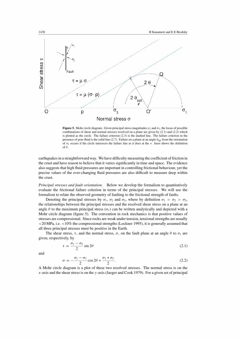
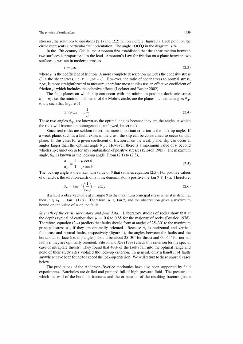
Figure 5. Mohr circle diagram. Given principal stress magnitudes σ1 and σ3, the locus of possiblecombinations of shear and normal stresses resolved on a plane are given by (2.1) and (2.2) whichis plotted as the circle. The failure criterion (2.3) is the dashed line. The failure criterion in thepresence of pore fluid is the solid line (2.7). Failure on a plane at an angle θopt from the orientationof σ1 occurs if the circle intersects the failure line as it does at the ∗. Inset shows the definitionof θ .
earthquakes in a straightforward way. We have difficulty measuring the coefficient of friction inthe crust and have reason to believe that it varies significantly in time and space. The evidencealso suggests that high fluid pressures are important in controlling frictional behaviour, yet theprecise values of the ever-changing fluid pressures are also difficult to measure deep withinthe crust.
Principal stresses and fault orientation. Below we develop the formalism to quantitativelyevaluate the frictional failure criterion in terms of the principal stresses. We will use theformalism to relate the observed geometry of faulting to the frictional strength of faults.
Denoting the principal stresses by σ1, σ2 and σ3, where by definition σ1 > σ2 > σ3,the relationships between the principal stresses and the resolved shear stress on a plane at anangle θ to the maximum principal stress (σ1) can be written analytically and depicted with aMohr circle diagram (figure 5). The convention in rock mechanics is that positive values ofstresses are compressional. Since rocks are weak under tension, tensional strengths are usually<20 MPa, i.e. <10% the compressional strengths (Lockner 1995), it is generally assumed thatall three principal stresses must be positive in the Earth.
The shear stress, τ , and the normal stress, σ , on the fault plane at an angle θ to σ1 aregiven, respectively, by
τ = σ1 − σ3
2sin 2θ (2.1)
and
σ = −σ1 − σ3
2cos 2θ +
σ1 + σ3
2. (2.2)
A Mohr circle diagram is a plot of these two resolved stresses. The normal stress is on thex-axis and the shear stress is on the y-axis (Jaeger and Cook 1979). For a given set of principal
The physics of earthquakes 1439
stresses, the solutions to equations (2.1) and (2.2) fall on a circle (figure 5). Each point on thecircle represents a particular fault orientation. The angle � OO′Q in the diagram is 2θ .
In the 17th century, Guillaume Amonton first established that the shear traction betweentwo surfaces is proportional to the load. Amonton’s Law for friction on a plane between twosurfaces is written in modern terms as
τ = µσ, (2.3)
where µ is the coefficient of friction. A more complete description includes the cohesive stressC in the shear stress, i.e. τ = µσ + C. However, the ratio of shear stress to normal stress,τ/σ , is more straightforward to measure, therefore most studies use an effective coefficient offriction µ which includes the cohesive effects (Lockner and Beeler 2002).
The fault planes on which slip can occur with the minimum possible deviatoric stressσ1 − σ3, i.e. the minimum diameter of the Mohr’s circle, are the planes inclined at angles θopt
to σ1, such that (figure 5)
tan 2θopt = ± 1
µ. (2.4)
These two angles θopt are known as the optimal angles because they are the angles at whichthe rock will fracture in homogeneous, unflawed, intact rock.
Since real rocks are seldom intact, the more important criterion is the lock-up angle. Ifa weak plane, such as a fault, exists in the crust, the slip can be constrained to occur on thatplane. In this case, for a given coefficient of friction µ on the weak plane, slip can occur atangles larger than the optimal angle θopt. However, there is a maximum value of θ beyondwhich slip cannot occur for any combination of positive stresses (Sibson 1985). The maximumangle, θlu, is known as the lock-up angle. From (2.1) to (2.3),
σ1
σ3= 1 + µ cot θ
1 − µ tan θ. (2.5)
The lock-up angle is the maximum value of θ that satisfies equation (2.5). For positive valuesof σ1 and σ3, the solution exists only if the denominator is positive, i.e. tan θ � 1/µ. Therefore,
θlu = tan−1
(1
µ
)= 2θopt. (2.6)
If a fault is observed to lie at an angle θ to the maximum principal stress when it is slipping,then θ � θlu = tan−1(1/µ). Therefore, µ � tan θ , and the observation gives a maximumbound on the value of µ on the fault.
Strength of the crust: laboratory and field data. Laboratory studies of rocks show that atthe depths typical of earthquakes µ = 0.6 to 0.85 for the majority of rocks (Byerlee 1978).Therefore, equation (2.4) predicts that faults should form at angles of 25–30˚ to the maximumprincipal stress σ1, if they are optimally oriented. Because σ1 is horizontal and verticalfor thrust and normal faults, respectively (figure 4), the angles between the faults and thehorizontal surface (i.e. dip angles) should be about 25–30˚ for thrust and 60–65˚ for normalfaults if they are optimally oriented. Sibson and Xie (1998) check this criterion for the specialcase of intraplate thrusts. They found that 40% of the faults fall into the optimal range andnone of their study sites violated the lock-up criterion. In general, only a handful of faultsanywhere have been found to exceed the lock-up criterion. We will return to these unusual casesbelow.
The predictions of the Anderson–Byerlee mechanics have also been supported by fieldexperiments. Boreholes are drilled and pumped full of high-pressure fluid. The pressure atwhich the wall of the borehole fractures and the orientation of the resulting fracture give a
1440 H Kanamori and E E Brodsky
measure of the magnitude and orientation of the least principal stress. More sophisticatedmethods use the hoop stress to infer the maximum principal stress. When these experimentsare performed in an area prone to normal faulting, i.e. where the maximum principal stress isvertical, the magnitude of the stresses resultant on the fracture plane and their orientation areconsistent with internal friction of 0.6 (Zoback and Healey 1984).
One complication to this simple picture was recognized early on. High fluid pressurescan support part of the load across a fault and reduce the friction. In the presence of fluidsequation (2.3) is modified to be
τ = µ(σ − p), (2.7)
where p is the pore pressure. Hubbert and Rubey (1959) first recognized the importance of thefluid effect on fault friction. Fluid pressure at a certain depth should theoretically be determinedby the weight of the water column above. This state is called hydrostatic. In the course oftheir work on oil exploration, Hubbert and Rubey observed that pressures in pockets of fluidsin the crust commonly exceeded hydrostatic pressure. They connected this observation withstudies of faulting and proposed that the pore pressure p at a depth can approach the normalstress σ on faults, resulting in low friction.
The most spectacular support for the importance of the Anderson–Byerlee paradigmof failure as modified by Hubbert and Rubey came from the 1976 Rangeley experiment.Earthquakes were induced by pumping water to increase the fluid pressure at depth in an oilfield with little surface indication of faulting (Raleigh et al 1976). Using equations (2.1), (2.2)and (2.7), the observed fault orientation, the observed values of σ1 and σ3 from in situ boreholeexperiments and the measured value of µ on rock samples from the site, the researcherssuccessfully predicted the increase in pore pressure that is necessary to trigger earthquakes.
Conflicting observations? The most controversial aspect of the Anderson–Byerleeformulation has been the applicability of the laboratory values of friction to natural settings.A fault that fails according to equation (2.7) with µ = 0.6–0.85 and hydrostatic fluid pressureis called a strong fault. Three lines of evidence have complicated the Andersonian picture andled researchers to question whether or not faults are strong before and during earthquakes.
The most often cited evidence against the strong fault hypothesis is based on heat flowdata. If µ is high, the frictional stress on the fault should generate heat. This heat generation,averaged over geological time should make a resolvably high level of heat flow if the depth-averaged shear stress is greater than 20 MPa. Lachenbruch and Sass (1980) showed that theSan Andreas fault generates no observable perturbation to the regional heat flow pattern. Someauthors have suggested that regional-scale groundwater flow may obscure such a signal, butrecent modelling has shown that the data are inconsistent with any known method of removingthe heat from the fault (Saffer et al 2003). Therefore, these difficult heat flow observationsstand as the best evidence that the San Andreas has a low resolved depth-averaged shear stress(�20 MPa). Since this stress is lower than that which can be achieved with hydrostatic porepressure and Byerlee friction, the fault is weak according to the definition at the beginningof this section. If the pore pressure is hydrostatic, the upper limit of 20 MPa shear stresscorresponds to a maximum value of µ of 0.17. The heat flow data is sensitive only to theresolved shear stress, rather than the value of µ. Pore pressures that are more than 2.3 timesthe hydrostatic values can also satisfy heat flow constraint without requiring small µ. The heatflow observations can not distinguish between high pore pressure and low intrinsic fault friction.
The second line of evidence comes from geological mapping. Low-angle normal faultshave now been robustly documented in the geological record (e.g. Wernicke (1981)). Althoughit is uncertain whether or not rapid slip occurred on these faults (as opposed to slow aseismic
The physics of earthquakes 1441
creep), it is clear that large-scale movement occurred on certain faults with dip angles of 20˚and perhaps as low as 2˚ (Axen 2004). If the faulting occurred at the lock-up angle in themore conservative case, the lock-up angle must be 70˚, which translates to µ = 0.4 from (2.6).Therefore, µ � 0.4 on the low-angle normal faults.
Note that high pore pressure does not affect the geological result, because combining (2.6)with (2.1) and (2.2) yields
σ1 − p
σ3 − p= 1 + µ cot θ
1 − µ tan θ(2.8)
and the lock-up angle is still tan−1(1/µ) as long as σ3 − p � 0. The only alternative is that p
exceeds the minimum principal stress and the left-hand side (lhs) of (2.8) is negative.A third line of evidence complicating the Anderson–Byerlee paradigm is that the maximum
principal stresses next to major strike-slip faults like the San Andreas in California and Nojimain Japan are sometimes nearly normal to the fault (Zoback et al 1987, Ikeda 2001, Provostand Houston 2003). On the creeping zone of the San Andreas in central California, Provostand Houston find that the angle θ between σ1 and the fault is ∼80˚. Therefore, according toequation (2.6) these areas must have µ < 0.2 in order to be able to support motion. Furthernorth on the fault, the angle θ varies from 40˚ to 70˚ implying a maximum value of µ varyingfrom 0.4 to 1.2 depending on location. In Southern California, Hardebeck and Hauksson(2001) find values of θ as low as 60˚. Once again, high pore pressures in the fault do notremove the need for a low value of µ in the places with high θ , if these measurements of highvalues of θ reflect the stress state directly on the fault. Both Byerlee (1992) and Rice (1992)argue that the stress orientation observations may not reflect the state of stress within the coreof a pressurized, fluid-filled fault. If it is true that the orientations are only measured outsidethe fault core, then there is no constraint on the fault stress from this line of evidence.
Summary. The overall picture that is emerging is a good deal more complicated than theAndersonian view. If the framework of equations (2.1), (2.2) and (2.7) is correct then inareas with large, mature faults it appears that the µ applicable for initiation of slip must besignificantly different from what is measured in the laboratory for intact rocks or immaturefaults like Rangely. Moreover, the stress orientation data hint that these variables may vary intime as well as space (Hardebeck and Hauksson 2001). Alternatively, pore pressure may beso high that it exceeds the minimum principal stress. However, increasing the pore pressurepresents new problems as rocks can fail under tension with relatively low differential stresses.An additional complication is that µ can depend on the slip rate and its history (Dieterich1979). Clearly, our simple criterion for earthquakes proposed above is insufficient to explainthis complexity of behaviour. In order to answer our question of why earthquakes begin, wewill have to dig deeper.
3. Quantifying earthquakes
In order to begin to answer these questions about earthquakes, we need to first review the majorobservational facts and the parameters we use to quantify earthquakes. The most developedmethod for measuring earthquakes is to measure the elastic wave-field generated by the suddenslip on a fault plane. Below, we discuss how the wave amplitude and frequencies are related tothe physical properties of the earthquake. We then list the most common earthquake parametersderived from the wave-field and discuss their dynamical significance. Finally we explore thescaling relationships between the observed parameters.
1442 H Kanamori and E E Brodsky
3.1. Earthquake source parameters and observables
A formal description of the elastic problem. An earthquake is a failure process in Earth’s crust.For a short-term process, we assume that the medium is elastic. We imagine that an earthquakeperturbs the stress field by relaxing the stress in a localized region S embedded in the elasticmedium. Prior to an earthquake, the crust is in equilibrium under some boundary conditionswith the initial displacement �u0(�r) and the stress distribution σ0(�r), where �r is the positionvector. The total potential energy (gravitational energy plus strain energy) of the system atthis stage is W0. In most seismological problems the displacement is assumed to be small andlinear elasticity theory is used. Then, at t = 0, i.e. the initiation time of an earthquake, a failureoccurs at a point in the medium called the earthquake hypocentre. Transient motion begins,energy is radiated, and rupture propagates into a region, S, representing the earthquake rupturezone. After the rupture propagation has stopped and the transient motion has subsided, thedisplacement and stress become �u1(�r) and σ1(�r). We denote the total potential energy of thisstate by W1. (Note that in section 2.2 subscripts 1, 2 and 3 are used to indicate the principalstresses; here, subscripts 0 and 1 are used to indicate the states before and after an earthquake,respectively.)
The processes in the source region S are modelled by a localized inelastic process whichrepresents the result of the combination of brittle rupture and plastic yielding. The seismicstatic displacement field �u(�r) is
�u(�r) = �u1(�r) − �u0(�r) (3.1)
and the stress drop is
σ(�r) = σ0(�r) − σ1(�r). (3.2)
The change in the potential energy is
W = W0 − W1. (3.3)
During the failure process (i.e. coseismic process), some energy is radiated (radiated energy,ER) and some energy is dissipated mechanically (fracture energy, EG) and thermally (thermalenergy, EH). Because some parts of the fracture energy eventually become thermal energy,the distinction between EG and EH is model dependent.
To study an earthquake process, at least three approaches are possible.
(1) Spontaneous failure. In this case, the modelled failure growth is controlled by failurecriterion (or failure physics) at each point in the medium. Thus, the final failure surface, orvolume, is determined by the failure process itself. This is the most physically desirable model,but it requires the knowledge of every detail of the structure and properties of the medium.Because it is difficult to gain this information in the crust, this approach is seldom taken.
(2) Dynamic failure on a prescribed source region. In this approach, we fix the geometry of thesource region. In most seismological problems, the source is a thin fault zone, and is modelledas a planar failure surface. Then what controls the rupture is the friction law on the faultplane (constitutive relation), and the elasto-dynamic equations are solved for a given frictionlaw (often parameterized) on the fault plane. The resulting displacement field is comparedwith the observed field to determine the fault friction law. This approach has been taken inrecent years as more computer power is available. (A recent review on this subject is given byMadariaga and Olsen (2002).)
(3) Kinematic model. In this approach, the wave-field is computed for a prescribed slip motionon the fault using the elastic dislocation theory. Then, the slip distribution on the fault isdetermined by the inversion of observed seismic data. At this stage, no source physics is
The physics of earthquakes 1443
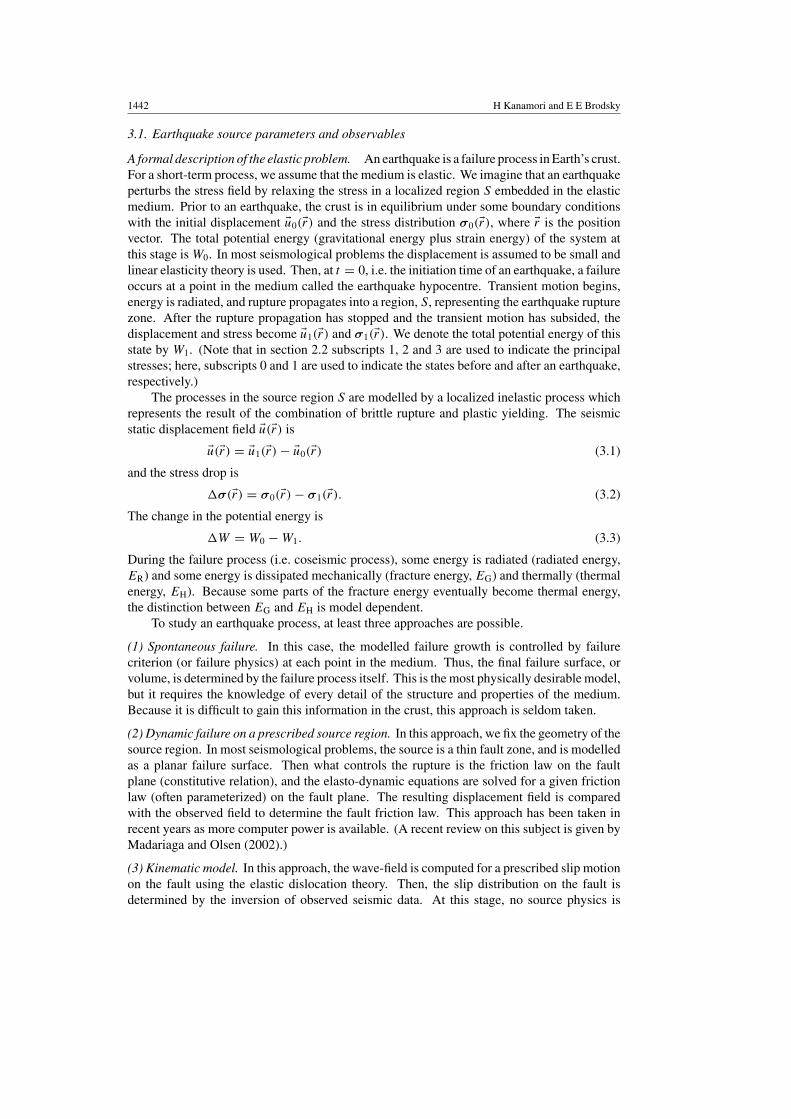
Figure 6. Representation of a dislocation (fault) seismic source. Left: a seismic fault representedby a shear displacement offset D over a surface with an area S, embedded in a medium withrigidity µ. Right: a force double couple equivalent to the dislocation model shown on left, in thelimit of point source (i.e. S → 0, and D → ∞ while the product DS remains finite).
invoked. In this sense, this approach is called kinematic. However, once the slip is determined,it can be used to compute the associated stress field. The displacement and the stress fieldon the fault plane, together, can be used to infer the physical process involved in failure (i.e.friction, etc). Since many methods for inversion of seismic data have been developed, thisapproach is widely used. (A recent review on this subject is also given by Madariaga andOlsen (2002).)
3.1.1. Seismic source and displacement field. First, consider a very small fault (i.e. pointsource) on which a displacement offset D (the difference between the displacements of thetwo sides of a fault) occurs (figure 6, left).
We want to find a set of forces that will generate a stress field equivalent to the stress fieldgenerated by a given imposed displacement on the fault. Since the fault is entirely enclosedby elastic crust and no work is done by external forces, both linear and angular momentummust be conserved during faulting. It can be shown that the force system that respects theseconservation laws and produces a stress field equivalent to the point dislocation source isthe combination of two perpendicular force couples (figure 6, right). This force system iscommonly called a double couple source. The moment of each force couple M0 is given by(Stekettee 1958, Maruyama 1964, Burridge and Knopoff 1964)
M0 = µDS, (3.4)
where µ is the rigidity of the material surrounding the fault. (Note that in section 2.2, µ isused for the coefficient of friction, but in this section it is used to represent the rigidity. In thelater sections µ is used both for the rigidity and the coefficient of friction. The distinction willbe clear from the text and context.) A finite fault model can be constructed by distributingthe point sources on a fault plane. The dimension of M0 is [force] × [length] = [energy]. Inseismology, it is common to use N m for the unit of M0, rather than J (joule), because M0 isthe moment of the equivalent force system, and does not directly represent any energy-relatedquantity of the source.
For simplicity, we consider a homogeneous whole space with the density, ρ, the P-wave(compressional wave) velocity, α and the S-wave (shear wave) velocity, β. In the absenceof any interfaces in the elastic medium, disturbances are propagated as simple elastic wavesknown as body waves. If a point source with seismic moment, M0(t), is placed at the origin,the displacement in the far-field is given in the polar coordinate, (r, θ, φ), asur
uθ
uφ
= 1
4πρrα3M ′
0
(t − r
α
) Rr(θ, φ)
00
+
1
4πρrβ3M ′
0
(t − r
β
) 0
Rθ(θ, φ)
Rφ(θ, φ)
, (3.5)
where the prime symbol denotes differentiation with respect to the argument.
1444 H Kanamori and E E Brodsky
Times (s)
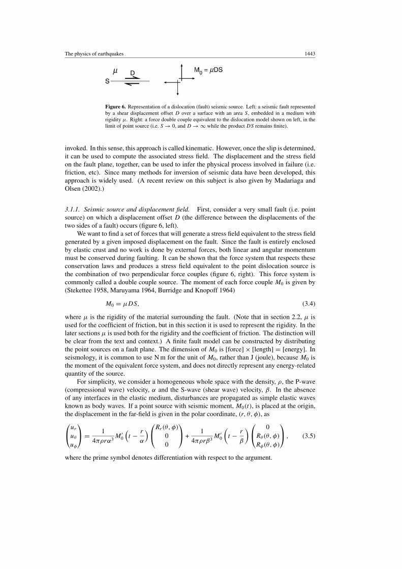
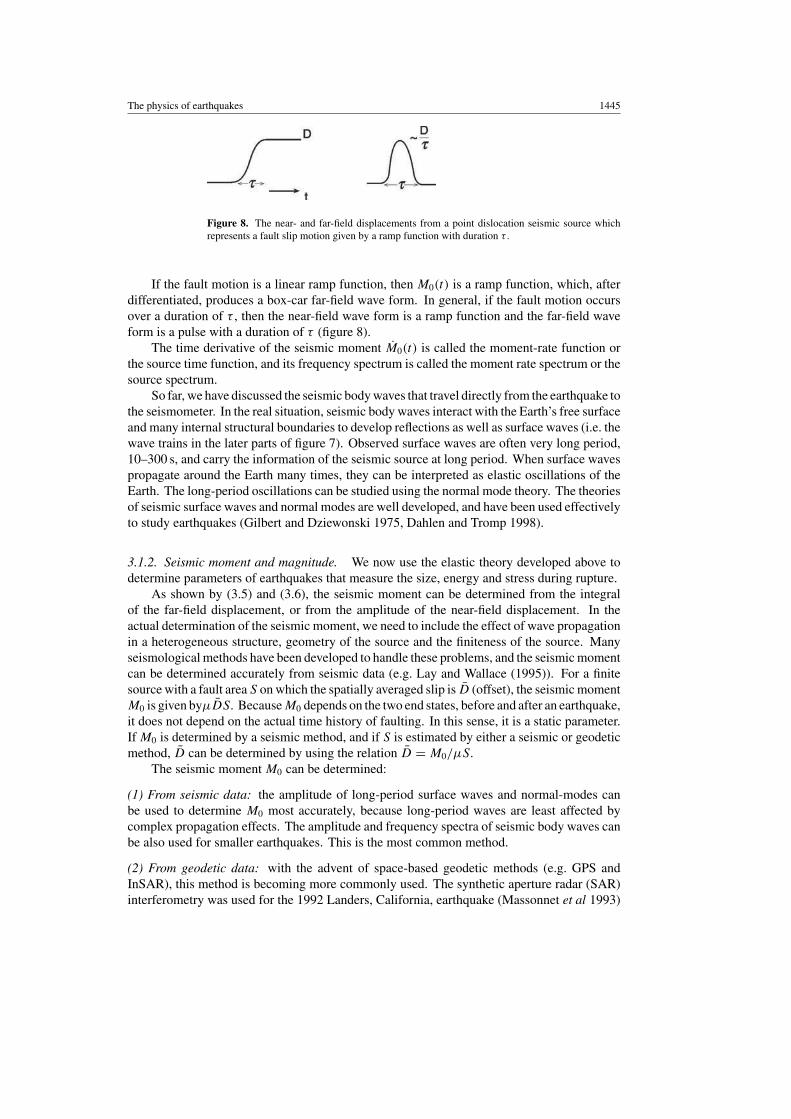
Figure 7. Example of displacement from the Mw = 7.9, 3 November 2002, Alaskaearthquake recorded by a broadband seismometer 3460 km away in Mammoth Lakes, California.The components are radial (R), transverse (T) and vertical (Z). The radial and transverse componentsare the two components on the horizontal plane. The early motion on these seismograms (between400 and 800 s) shows P- and S-waves described by (3.5). Later motion (after 800 s) shows surfacewaves produced by the interactions of the waves with boundaries in the earth and heterogeneousstructure.
The first term is the P-wave and the second term, S-wave. Rr(θ, φ), Rθ(θ, φ) and Rφ(θ, φ)
represent the radiation patterns, which depend on the geometry of the source and the observationpoint. (For more details, see, e.g. Lay and Wallace (1995), Aki and Richards (2002).) Thesedisplacement components are what are measured by seismometers (figure 7).
At short distances from the source, we have an additional term representing the near-fielddisplacement. The primary component of the near-field displacement is given approximately by
u ∝ 1
4πµr2M0(t). (3.6)
The near-field displacement is important for the determination of detailed spatial and temporaldistribution of slip in the rupture zone. Far away from the fault, (3.6) is negligible as it fallsoff much more quickly than the far-field terms (1/r2 as opposed to 1/r). The reason why thenear-field and far-field displacements are proportional to M0(t)/r2 and M ′
0(t)/r , respectively,is that the near-field is essentially determined by the motion on one side of the fault, whilethe far-field represents the contributions from both sides of the fault. This situation is similarto that of an electric field from a point charge and a dipole. (For more details, see Aki andRichards (2002)).
The physics of earthquakes 1445
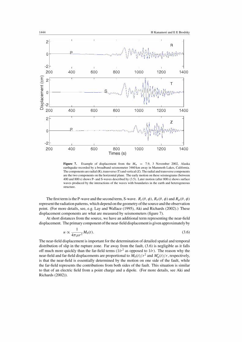
Figure 8. The near- and far-field displacements from a point dislocation seismic source whichrepresents a fault slip motion given by a ramp function with duration τ .
If the fault motion is a linear ramp function, then M0(t) is a ramp function, which, afterdifferentiated, produces a box-car far-field wave form. In general, if the fault motion occursover a duration of τ , then the near-field wave form is a ramp function and the far-field waveform is a pulse with a duration of τ (figure 8).
The time derivative of the seismic moment M0(t) is called the moment-rate function orthe source time function, and its frequency spectrum is called the moment rate spectrum or thesource spectrum.
So far, we have discussed the seismic body waves that travel directly from the earthquake tothe seismometer. In the real situation, seismic body waves interact with the Earth’s free surfaceand many internal structural boundaries to develop reflections as well as surface waves (i.e. thewave trains in the later parts of figure 7). Observed surface waves are often very long period,10–300 s, and carry the information of the seismic source at long period. When surface wavespropagate around the Earth many times, they can be interpreted as elastic oscillations of theEarth. The long-period oscillations can be studied using the normal mode theory. The theoriesof seismic surface waves and normal modes are well developed, and have been used effectivelyto study earthquakes (Gilbert and Dziewonski 1975, Dahlen and Tromp 1998).
3.1.2. Seismic moment and magnitude. We now use the elastic theory developed above todetermine parameters of earthquakes that measure the size, energy and stress during rupture.
As shown by (3.5) and (3.6), the seismic moment can be determined from the integralof the far-field displacement, or from the amplitude of the near-field displacement. In theactual determination of the seismic moment, we need to include the effect of wave propagationin a heterogeneous structure, geometry of the source and the finiteness of the source. Manyseismological methods have been developed to handle these problems, and the seismic momentcan be determined accurately from seismic data (e.g. Lay and Wallace (1995)). For a finitesource with a fault area S on which the spatially averaged slip is D (offset), the seismic momentM0 is given byµDS. Because M0 depends on the two end states, before and after an earthquake,it does not depend on the actual time history of faulting. In this sense, it is a static parameter.If M0 is determined by a seismic method, and if S is estimated by either a seismic or geodeticmethod, D can be determined by using the relation D = M0/µS.
The seismic moment M0 can be determined:
(1) From seismic data: the amplitude of long-period surface waves and normal-modes canbe used to determine M0 most accurately, because long-period waves are least affected bycomplex propagation effects. The amplitude and frequency spectra of seismic body waves canbe also used for smaller earthquakes. This is the most common method.
(2) From geodetic data: with the advent of space-based geodetic methods (e.g. GPS andInSAR), this method is becoming more commonly used. The synthetic aperture radar (SAR)interferometry was used for the 1992 Landers, California, earthquake (Massonnet et al 1993)
1446 H Kanamori and E E Brodsky
Table 1. Seismic moment determinations from different data sets.
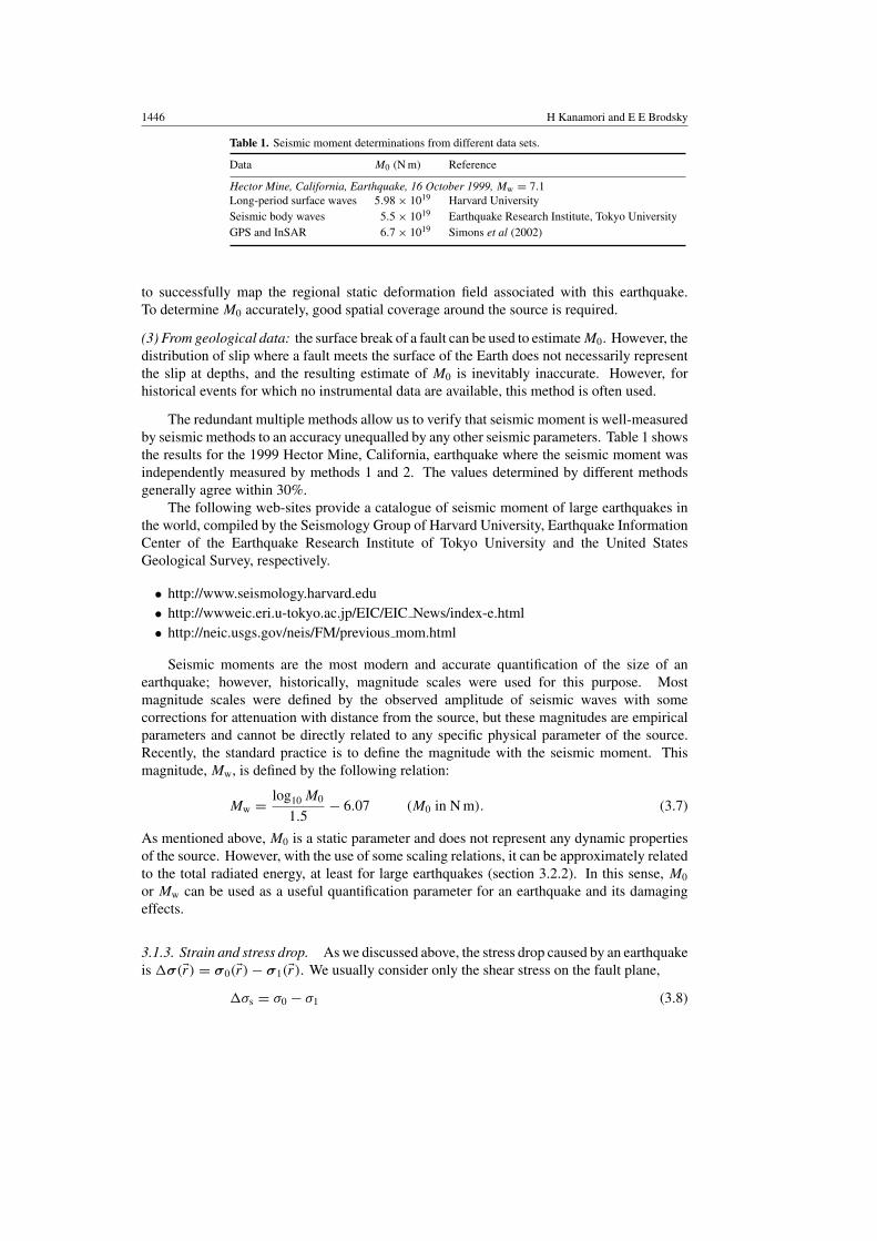
Data M0 (N m) Reference
Hector Mine, California, Earthquake, 16 October 1999, Mw = 7.1Long-period surface waves 5.98 × 10¹⁹ Harvard UniversitySeismic body waves 5.5 × 10¹⁹ Earthquake Research Institute, Tokyo UniversityGPS and InSAR 6.7 × 10¹⁹ Simons et al (2002)
to successfully map the regional static deformation field associated with this earthquake.To determine M0 accurately, good spatial coverage around the source is required.
(3) From geological data: the surface break of a fault can be used to estimate M0. However, thedistribution of slip where a fault meets the surface of the Earth does not necessarily representthe slip at depths, and the resulting estimate of M0 is inevitably inaccurate. However, forhistorical events for which no instrumental data are available, this method is often used.
The redundant multiple methods allow us to verify that seismic moment is well-measuredby seismic methods to an accuracy unequalled by any other seismic parameters. Table 1 showsthe results for the 1999 Hector Mine, California, earthquake where the seismic moment wasindependently measured by methods 1 and 2. The values determined by different methodsgenerally agree within 30%.
The following web-sites provide a catalogue of seismic moment of large earthquakes inthe world, compiled by the Seismology Group of Harvard University, Earthquake InformationCenter of the Earthquake Research Institute of Tokyo University and the United StatesGeological Survey, respectively.
• http://www.seismology.harvard.edu• http://wwweic.eri.u-tokyo.ac.jp/EIC/EIC News/index-e.html• http://neic.usgs.gov/neis/FM/previous mom.html
Seismic moments are the most modern and accurate quantification of the size of anearthquake; however, historically, magnitude scales were used for this purpose. Mostmagnitude scales were defined by the observed amplitude of seismic waves with somecorrections for attenuation with distance from the source, but these magnitudes are empiricalparameters and cannot be directly related to any specific physical parameter of the source.Recently, the standard practice is to define the magnitude with the seismic moment. Thismagnitude, Mw, is defined by the following relation:
Mw = log10 M0
1.5− 6.07 (M0 in N m). (3.7)
As mentioned above, M0 is a static parameter and does not represent any dynamic propertiesof the source. However, with the use of some scaling relations, it can be approximately relatedto the total radiated energy, at least for large earthquakes (section 3.2.2). In this sense, M0
or Mw can be used as a useful quantification parameter for an earthquake and its damagingeffects.
3.1.3. Strain and stress drop. As we discussed above, the stress drop caused by an earthquakeis σ(�r) = σ0(�r) − σ1(�r). We usually consider only the shear stress on the fault plane,
σs = σ0 − σ1 (3.8)

The physics of earthquakes 1447
and call it the static stress drop associated with an earthquake. The strain drop εs is given byεs = σs/µ. In general, σs varies spatially on the fault. The spatial average is given by
σs = 1
S
∫S
σs dS. (3.9)
Since the stress and strength distributions near a fault are non-uniform, the slip and stressdrop are, in general, complex functions of space. In most applications, we use the stressdrop averaged over the entire fault plane. The stress drop can be locally much higher than theaverage. To be exact, the average stress drop is the spatial average of the stress drop, as given by(3.9). However, the limited resolution of seismological methods often allows determinationsof only the average displacement over the fault plane, which in turn is used to compute theaverage stress drop. With this approximation, we estimate σs simply by
σs ≈ CµD
L, (3.10)
where, D is the average slip (offset), L is a characteristic rupture dimension, often definedby
√S and C is a geometric constant of order unity. Unfortunately, given the limited spatial
resolution of seismic data, we cannot fully assess the validity of this approximation. However,Madariaga (1977, 1979), Rudnicki and Kanamori (1981) and Das (1988) show that this is agood approximation unless the variation of stress on the fault is extremely large.
We often use σs to mean the average static stress drop in this sense. Some earlydeterminations of stress (strain) drops were made using D and L estimated from geodeticdata (e.g. 1927 Tango earthquake, Tsuboi (1933)).
More commonly, if the seismic moment is determined by either geodetic or seismologicalmethods, we use the following expression. Using M0 = µDS, L = S1/2 and (3.10), we canwrite
σs = CM0L−3 = CM0S
−3/2. (3.11)
If the length scale of the source is estimated from the geodetic data, aftershock area, tsunamisource area or other data, we can estimate the stress drop using (3.11) (e.g. Kanamori andAnderson (1975), Abercrombie and Leary (1993)).
If the slip distribution on the fault plane can be determined from high-resolution seismicdata, it is possible to estimate the stress drop on the fault plane (Bouchon 1997).
Since σs ≈ CM0L−3, an uncertainty in the length scale can cause a large uncertainty in
σs: a factor of 2 uncertainty in L results in a factor of 8 uncertainty in σs. Thus, an accuratedetermination of earthquake source size, either S or L, is extremely important in determiningthe stress drop.
3.1.4. Energy
Radiated energy, ER. The energy radiated by seismic waves, ER, is another importantphysical parameter of an earthquake. In principle, if we can determine the wave-fieldcompletely, it is straightforward to estimate the radiated energy. For example, if the P-wavedisplacement in a homogeneous medium is given by ur(r, t), then the energy radiated in aP-wave is given by
ER,α = ρα
∫S0
∫ +∞
−∞ur (r, t)
2 dt dS0, (3.12)
where S0 is a spherical surface at a large distance surrounding the source. Similarly, the energyradiated in an S-wave is given by
ER,β = ρβ
∫S0
∫ +∞
−∞[uθ (r, t)
2 + uφ(r, t)2] dt dS0. (3.13)

1448 H Kanamori and E E Brodsky
Table 2. Determinations of radiated energy with different data sets and methods.
Data ER (J) Reference
Bhuji, India, Earthquake, 26 January 2001, Mw = 7.6Regional data 2.1 × 10¹⁶ Singh et al (2004)Teleseismic data 2.0 × 10¹⁶ Venkataraman and Kanamori (2004)Frequency-domain method 1.9 × 10¹⁶ Singh et al (2004)
Hector Mine, California, Earthquake, 16 October 1999, Mw = 7.1Regional data 3.4 × 10¹⁵ Boatwright et al (2002)
3 × 10¹⁵ Venkataraman et al (2002)Teleseismic data 3.2 × 10¹⁵ Boatwright et al (2002)
2 × 10¹⁵ Venkataraman et al (2002)
The total energy, ER, is the sum of ER,α and ER,β (e.g. Haskell (1964)). In practice, however,the wave-field in the Earth is extremely complex because of the complexity of the seismicsource, propagation effects, attenuation and scattering. Extensive efforts have been made inrecent years to accurately determine ER. For earthquakes for which high-quality seismic dataare available, ER can be estimated probably within a factor of 2–3 (McGarr and Fletcher 2002).Some examples are shown in table 2.
Potential energy. The potential energy change in the crust due to an earthquake is
W = 12 (σ0 + σ1)DS, (3.14)
where the bar stands for the spatial average (Kostrov 1974, Dahlen 1977). Equation (3.14) canbe rewritten as,
W = 12 (σ0 − σ1)DS + σ1DS = 1
2σsDS + σ1DS = W0 + σ1DS, (3.15)
where
W0 = 12σsDS. (3.16)
Two difficulties are encountered. First, with seismological measurements alone, the absolutevalue of the stresses, σ0 and σ1 cannot be determined. Only the difference σs = σ0 − σ1 isdetermined. Thus, we cannot compute W from seismic data. As we discussed in section 2.2,non-seismological methods give inconsistent results for background stress. Second, as wediscussed in section 3.1.3 for the stress drop, with the limited resolution of seismologicalmethods, the details of spatial variation of stress and displacement cannot be determined.Thus we commonly use, instead of (3.16),
W0 = 12σs DS. (3.17)
Unfortunately, it is not possible to accurately assess the errors associated with theapproximation of equation (3.17). It is a common practice to assume that the approximationis sufficiently accurate if the spatial variation is not very rapid.
Although W cannot be determined by seismological methods, W0 can be computedfrom the seismologically determined parameters, σs, D and S. In general σ1DS > 0, unlessa large scale overshoot occurs, and W0 can be used as a lower bound of W . If the residualstress σ1 is small, W0 is a good approximation ofW .
It is important to note that we can determine two kinds of energies, the radiated energy(ER) and the lower bound of the potential energy change (W0), with seismological dataand methods. These two energies play an important role in understanding the physics ofearthquakes (section 4.4).
The physics of earthquakes 1449
3.1.5. Rupture mode, speed and directivity. Another observable feature of earthquakes is therupture pattern on the fault. Although the rupture pattern is not a parameter sensu stricto, sinceit is not a single summary quantity, it is another observable characterization of the rupture. Fromthe rupture patterns we can define some secondary parameters describing rupture propagationvelocity, slip duration and directivity.
An earthquake occurs on a finite fault. It initiates from a point, called a hypocentre, andpropagates outward on the fault plane. From the gross rupture patterns, we classify the rupturepatterns into unilateral rupture, bilateral rupture and two-dimensional (approximately circular)rupture patterns. In a unilateral rupture, the hypocentre is at the one end of the fault, and therupture propagates primarily in one direction toward the other end. One good example is therecent Denali, Alaska, earthquake (Mw = 7.9, 3 November 2002). In a bilateral rupture,the rupture propagates in opposite directions from the hypocentre. Good examples include the1989 Loma Prieta, California, earthquake (Mw = 6.9), and the 1995 Kobe, Japan, earthquake(Mw = 6.9). Bilateral ruptures are not necessarily symmetric. The 1906 San Francisco,California, earthquake is believed to have ruptured in both directions, but propagated furtherto the north than the south. In the description of unilateral and the bilateral fault, the faultgeometry is assumed to be one-dimensional. In some earthquakes, the rupture propagates inall directions on the fault plane. In these cases, a circular fault is often used to model the faultplane.
Directivity and source duration. The source finiteness and rupture propagation have animportant effect on seismic radiation. This effect, called directivity, is similar to the Dopplereffect.
As we discussed in section 3.1.1, the far-field displacement is given by the time derivativeof the near-field displacement and is pulse-like. However, because of the Doppler effect,the observer located in the direction of the rupture will see a shorter pulse than the observerin the direction away from the rupture direction. However, the area under the pulse-likewaveform (i.e. the displacement integrated over time) is constant, regardless of the azimuthand is proportional to the seismic moment, M0. The duration of the pulse, τ , when averagedover the azimuth, is proportional to the length scale of the fault L divided by the rupture speed, V
τ = L
V. (3.18)
For unilateral, bilateral and circular faults, L is commonly taken to represent the fault length,half the fault length and the radius of the fault plane, in that order. The variation of the pulsewidth as a function of azimuth due to rupture propagation has an important influence on groundmotions. As mentioned above, at a site towards the rupture propagation, the pulse becomeslarger and narrower, and produces stronger ground motions which often result in heavier shak-ing damage, than at a site away from the rupture propagation. A good example is the 1995Kobe, Japan, earthquake. The rupture of one of the bilateral segments propagated northeastfrom the hypocentre toward Kobe and produced very strong ground motions in the city.
Rupture speed. As we will discuss later (section 4.6.1), the rupture speed is an importantparameter which reflects the dynamic characteristic of a fracture. In particular, the fraction ofthe shear velocity that the shear crack rupture velocity achieves is related to the fracture energy.Thus it is important to determine the rupture speed of earthquake faulting to understand thenature of earthquake mechanics.
The rupture speed V has been determined for many large earthquakes. In general, for mostlarge shallow earthquakes, V is approximately 75–95% of the S-wave velocity at the depthwhere the largest slip occurred. However, there are some exceptions. For some earthquakes
1450 H Kanamori and E E Brodsky
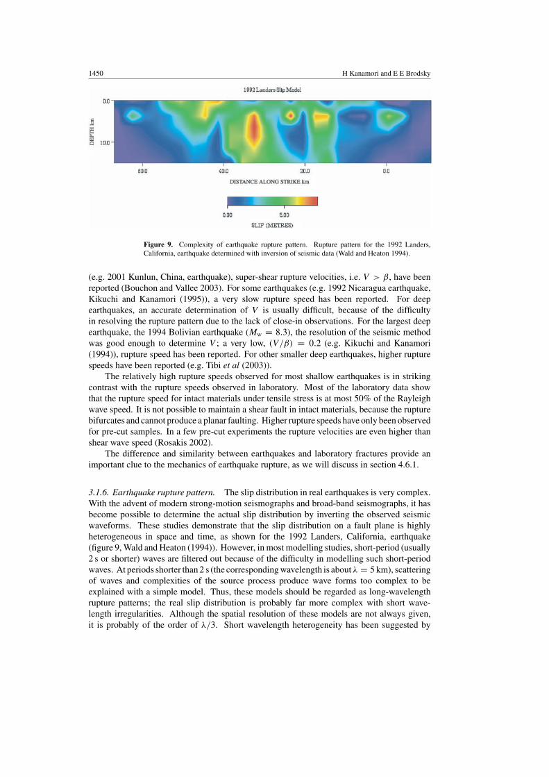
Figure 9. Complexity of earthquake rupture pattern. Rupture pattern for the 1992 Landers,California, earthquake determined with inversion of seismic data (Wald and Heaton 1994).
(e.g. 2001 Kunlun, China, earthquake), super-shear rupture velocities, i.e. V > β, have beenreported (Bouchon and Vallee 2003). For some earthquakes (e.g. 1992 Nicaragua earthquake,Kikuchi and Kanamori (1995)), a very slow rupture speed has been reported. For deepearthquakes, an accurate determination of V is usually difficult, because of the difficultyin resolving the rupture pattern due to the lack of close-in observations. For the largest deepearthquake, the 1994 Bolivian earthquake (Mw = 8.3), the resolution of the seismic methodwas good enough to determine V ; a very low, (V/β) = 0.2 (e.g. Kikuchi and Kanamori(1994)), rupture speed has been reported. For other smaller deep earthquakes, higher rupturespeeds have been reported (e.g. Tibi et al (2003)).
The relatively high rupture speeds observed for most shallow earthquakes is in strikingcontrast with the rupture speeds observed in laboratory. Most of the laboratory data showthat the rupture speed for intact materials under tensile stress is at most 50% of the Rayleighwave speed. It is not possible to maintain a shear fault in intact materials, because the rupturebifurcates and cannot produce a planar faulting. Higher rupture speeds have only been observedfor pre-cut samples. In a few pre-cut experiments the rupture velocities are even higher thanshear wave speed (Rosakis 2002).
The difference and similarity between earthquakes and laboratory fractures provide animportant clue to the mechanics of earthquake rupture, as we will discuss in section 4.6.1.
3.1.6. Earthquake rupture pattern. The slip distribution in real earthquakes is very complex.With the advent of modern strong-motion seismographs and broad-band seismographs, it hasbecome possible to determine the actual slip distribution by inverting the observed seismicwaveforms. These studies demonstrate that the slip distribution on a fault plane is highlyheterogeneous in space and time, as shown for the 1992 Landers, California, earthquake(figure 9, Wald and Heaton (1994)). However, in most modelling studies, short-period (usually2 s or shorter) waves are filtered out because of the difficulty in modelling such short-periodwaves. At periods shorter than 2 s (the corresponding wavelength is about λ = 5 km), scatteringof waves and complexities of the source process produce wave forms too complex to beexplained with a simple model. Thus, these models should be regarded as long-wavelengthrupture patterns; the real slip distribution is probably far more complex with short wave-length irregularities. Although the spatial resolution of these models are not always given,it is probably of the order of λ/3. Short wavelength heterogeneity has been suggested by
The physics of earthquakes 1451
complex high-frequency wave forms seen on accelerograms recorded at short distances. Zenget al (1994) modelled an earthquake fault as a fractal distribution of patches. This complexitysuggests that the microscopic processes on a fault plane can be important in controlling therupture dynamics, as we will discuss in section 4.5.
3.2. Seismic scaling relations
Now that we have measured some average properties of rupture, we need to relate theparameters to each other. The scaling relationships between the macroscopic source parametersare useful for isolating general constraints on the microscopic forces and processes in the faultzone during rupture. We will first discuss a selection of the observed scalings with only acursory overview of the implications. A more detailed discussion of microscopic physicsfollows in section 4.
3.2.1. Scaling relations for static parameters. The seismic moment, M0, is the sourceparameter that can be determined most reliably. Thus, it is useful to investigate a scalingrelation between M0 and another parameter that can be determined most directly from seismicobservations.
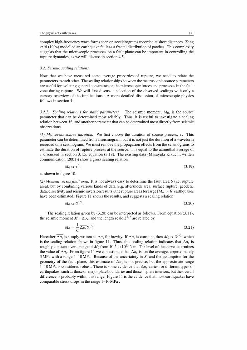
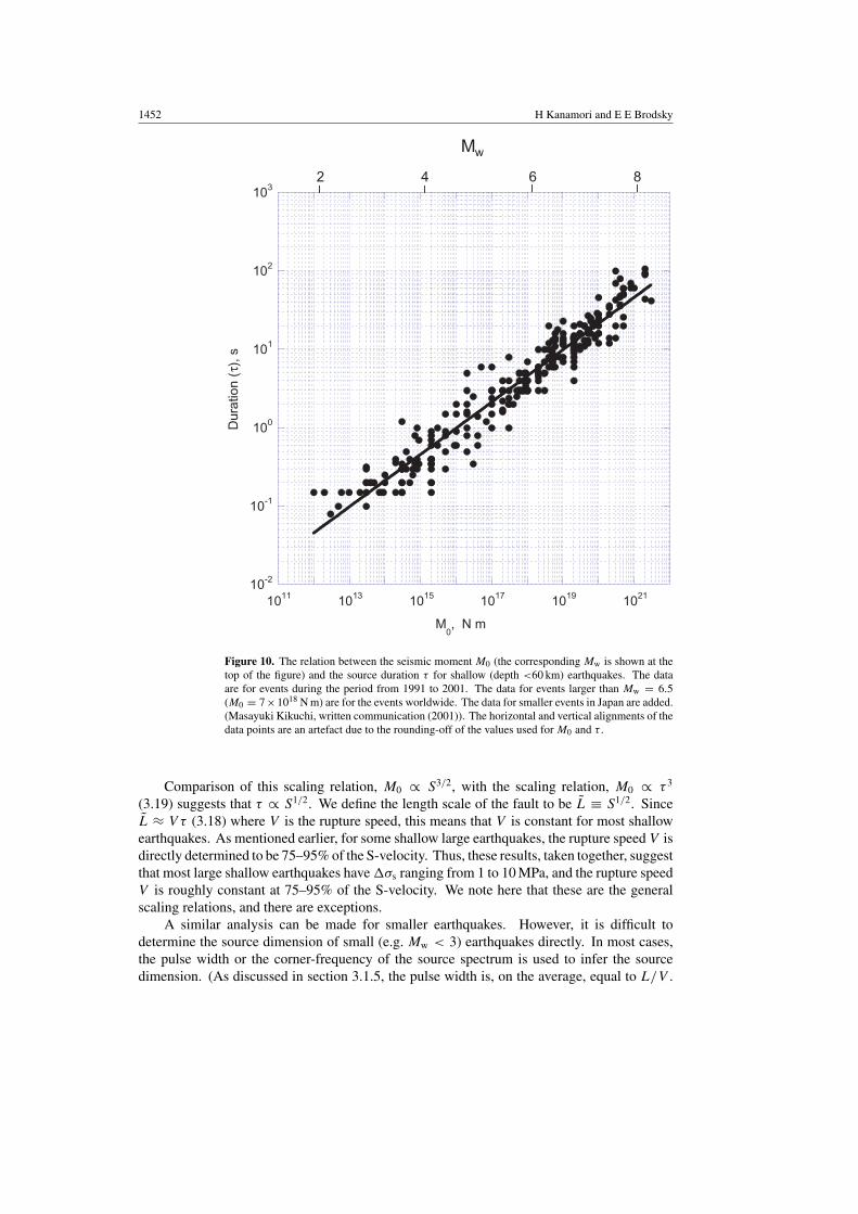
(1) M0 versus source duration. We first choose the duration of source process, τ . Thisparameter can be determined from a seismogram, but it is not just the duration of a waveformrecorded on a seismogram. We must remove the propagation effects from the seismograms toestimate the duration of rupture process at the source. τ is equal to the azimuthal average ofτ discussed in section 3.1.5, equation (3.18). The existing data (Masayuki Kikuchi, writtencommunication (2001)) show a gross scaling relation
M0 ∝ τ 3, (3.19)
as shown in figure 10.
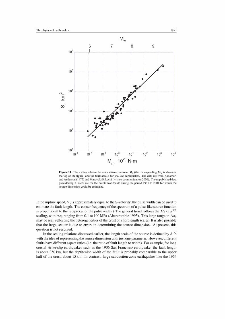
(2) Moment versus fault area. It is not always easy to determine the fault area S (i.e. rupturearea), but by combining various kinds of data (e.g. aftershock area, surface rupture, geodeticdata, directivity and seismic inversion results), the rupture areas for large (Mw > 6) earthquakeshave been estimated. Figure 11 shows the results, and suggests a scaling relation
M0 ∝ S3/2. (3.20)
The scaling relation given by (3.20) can be interpreted as follows. From equation (3.11),the seismic moment M0, σs, and the length scale S1/2 are related by
M0 = 1
CσsS
3/2. (3.21)
Hereafter σs is simply written as σs for brevity. If σs is constant, then M0 ∝ S3/2, whichis the scaling relation shown in figure 11. Thus, this scaling relation indicates that σs isroughly constant over a range of M0 from 1018 to 1023 N m. The level of the curve determinesthe value of σs. From figure 11 we can estimate that σs is, on the average, approximately3 MPa with a range 1–10 MPa. Because of the uncertainty in S, and the assumption for thegeometry of the fault plane, this estimate of σs is not precise, but the approximate range1–10 MPa is considered robust. There is some evidence that σs varies for different types ofearthquakes, such as those on major plate boundaries and those in plate interiors, but the overalldifference is probably within this range. Figure 11 is the evidence that most earthquakes havecomparable stress drops in the range 1–10 MPa .
1452 H Kanamori and E E Brodsky
10-2
10-1
100
101
102
103
1011 1013 1015 1017 1019 1021
Dur
atio
n (
τ), s
M0, N m
Mw
8642
Figure 10. The relation between the seismic moment M0 (the corresponding Mw is shown at thetop of the figure) and the source duration τ for shallow (depth <60 km) earthquakes. The dataare for events during the period from 1991 to 2001. The data for events larger than Mw = 6.5(M0 = 7×10¹⁸ N m) are for the events worldwide. The data for smaller events in Japan are added.(Masayuki Kikuchi, written communication (2001)). The horizontal and vertical alignments of thedata points are an artefact due to the rounding-off of the values used for M0 and τ .
Comparison of this scaling relation, M0 ∝ S3/2, with the scaling relation, M0 ∝ τ 3
(3.19) suggests that τ ∝ S1/2. We define the length scale of the fault to be L ≡ S1/2. SinceL ≈ V τ (3.18) where V is the rupture speed, this means that V is constant for most shallowearthquakes. As mentioned earlier, for some shallow large earthquakes, the rupture speed V isdirectly determined to be 75–95% of the S-velocity. Thus, these results, taken together, suggestthat most large shallow earthquakes have σs ranging from 1 to 10 MPa, and the rupture speedV is roughly constant at 75–95% of the S-velocity. We note here that these are the generalscaling relations, and there are exceptions.
A similar analysis can be made for smaller earthquakes. However, it is difficult todetermine the source dimension of small (e.g. Mw < 3) earthquakes directly. In most cases,the pulse width or the corner-frequency of the source spectrum is used to infer the sourcedimension. (As discussed in section 3.1.5, the pulse width is, on the average, equal to L/V .
The physics of earthquakes 1453
6 7 8 9
101
102
103
104
105
106
10-3 10-2 10-1 100 101 102 103 104
S,
km2
M0, 1020 N m
Mw
Figure 11. The scaling relation between seismic moment M0 (the corresponding Mw is shown atthe top of the figure) and the fault area S for shallow earthquakes. The data are from Kanamoriand Anderson (1975) and Masayuki Kikuchi (written communication 2001). The unpublished dataprovided by Kikuchi are for the events worldwide during the period 1991 to 2001 for which thesource dimension could be estimated.
If the rupture speed, V , is approximately equal to the S-velocity, the pulse width can be used toestimate the fault length. The corner frequency of the spectrum of a pulse-like source functionis proportional to the reciprocal of the pulse width.) The general trend follows the M0 ∝ S3/2
scaling, with σs ranging from 0.1 to 100 MPa (Abercrombie 1995). This large range in σs
may be real, reflecting the heterogeneities of the crust on short length scales. It is also possiblethat the large scatter is due to errors in determining the source dimension. At present, thisquestion is not resolved.
In the scaling relations discussed earlier, the length scale of the source is defined by S1/2
with the idea of representing the source dimension with just one parameter. However, differentfaults have different aspect ratios (i.e. the ratio of fault length to width). For example, for longcrustal strike-slip earthquakes such as the 1906 San Francisco earthquake, the fault lengthis about 350 km, but the depth-wise width of the fault is probably comparable to the upperhalf of the crust, about 15 km. In contrast, large subduction-zone earthquakes like the 1964
1454 H Kanamori and E E Brodsky
Alaskan earthquake have a fault width as large as 200 km or more. In view of this variationin aspect ratio, several investigators tried to investigate the scaling relation between M0 and L
(e.g. Romanowicz and Rundle (1993), Scholz (1994), Romanowicz and Ruff (2002)). Severaldifferent scaling relations, such as M0 ∝ L3/2 and M0 ∝ L2, have been proposed for differenttypes of earthquakes and for different magnitude ranges.
3.2.2. Scaling relations for dynamic parameters. The radiated energy, ER, is anothermacroscopic earthquake source parameter that can be determined by seismological methods(see section 3.1.4). The ratio
e = ER
M0= 1
µ
ER
DS(3.22)
has long been used in seismology as a useful parameter that characterizes the dynamicproperties of an earthquake (Aki 1966, Wyss and Brune 1968). The ratio e multiplied by therigidity µ is called the apparent stress. From (3.22), the ratio can be interpreted as proportionalto the energy radiated per unit fault area and per unit slip. In this sense, this scaling relationrepresents a dynamic property of earthquakes. As we will discuss later (section 4.4), if the staticstress drop is constant, then e must be constant if small and large earthquakes are dynamicallysimilar. Seismologists are very concerned with whether or not earthquakes are dynamicallysimilar because of the implications of the observation for the predictability of the eventual sizeof an earthquake. If small and large earthquakes are dynamically similar, then the initiationprocess is scale-invariant and therefore the size of earthquakes is inherently unpredictable.However, the converse statement is not true, so the observation of a lack of similarity cannotprove the predictability of earthquake size.
In view of its importance for understanding the dynamic character of earthquakes, manystudies have been devoted to the determination of e. Unfortunately, it is difficult to determineER accurately, because of the complex wave propagation effects in the Earth, especially forsmall earthquakes, and the results were widely scattered.
Recent improvements in data quality and methodology have significantly improved theaccuracy of ER determination for large earthquakes (e.g. Mw > 6) (e.g. Boatwright andChoy (1986), Boatwright et al (2002), Venkataraman et al (2002)). For small earthquakes, it isstill difficult because the relatively high-frequency seismic waves excited by small earthquakesare easily scattered and attenuated by the complex rock structures between the fault and aseismic station. Nevertheless, using down-hole instruments, or with the careful removal ofpath effects, large amounts of high-quality data for small earthquakes have been accumulated(Abercrombie 1995, Mayeda and Walter 1996, Izutani and Kanamori 2001, Prejean andEllsworth 2001, Kinoshita and Ohike 2002). The ratio depends on many seismogenicproperties of the source region so that it varies significantly for earthquakes in differenttectonic environments, such as continental crust, subduction zone, deep seismic zone, etc (Choyand Boatwright 1995, Perez-Campos and Beroza 2001, Venkataraman and Kanamori 2004).However, the data for the same type of earthquakes exhibit an interesting trend. Figure 12shows the results for crustal earthquakes in California and Japan.
Taken at face value, despite the large scatter, the average ratio e decreases as the magnitude,Mw, decreases. For large earthquakes (Mw ≈ 7), e is, on the average, approximately 5×10⁻⁵,but it is approximately a factor of 10 smaller at Mw ≈ 3, and a factor of 100 smaller atMw ≈ 1. Results for even smaller earthquakes show even smaller values of e (e.g. Jost et al(1998), Richardson and Jordan (2002)). Ide and Beroza (2001) suggested that many of thepublished e versus Mw relations could be biased to have decreased e for small events because ofinadequate corrections for path effects or the limited instrumental pass-band. These systematic

The physics of earthquakes 1455
10-8
10-7
10-6
10-5
10-4
10-3
0 1 2 3 4 5 6 7 8
Mayeda and Walter [1996]Abercrombie [1995]TERRAscope
Izutani and Kanamori [2001]Large Eqs
ER/M
0
Mw
Figure 12. The relation between e = ER/M0 and Mw (Abercrombie 1995, Mayeda and Walter1996, Izutani and Kanamori 2001, Kanamori et al (1993), for TERRAscope data).
measurement errors could mean that the real e is scale-independent. At present, this questionremains unresolved. If future research finds that e varies as suggested by figure 12, then theobservation would imply that large and small earthquakes are dynamically different.
4. Rupture processes
We have now provided an overview of the stresses that generate earthquakes along with adiscussion of the measurable parameters and their interrelationships. The next step in ourinquiry into why earthquakes happen is to examine the rupture process itself.
4.1. Fracture mechanics
To interpret seismological data, crack models are often used in part because the theories oncracks have been developed well. On the other hand, seismic faulting may be more intuitivelyviewed as sliding on a frictional surface (fault) where the physics of friction, especially stickslip, plays a key role. Seismic faulting in the Earth can be complex and we may require amixture of crack models and sliding models, or even other models to interpret it. Despite thiscomplexity, crack models and frictional sliding models provide a useful framework for theinterpretation of earthquake processes. Here, we limit our discussion to the very basic aspectsof these models.
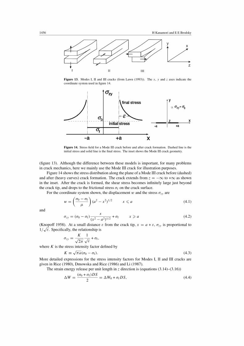
4.1.1. An overview of the crack model. In crack mechanics, three types of crack geometries,Mode I (tensile), Mode II (longitudinal shear) and Mode III (transverse shear), are used
1456 H Kanamori and E E Brodsky
z
xy
Figure 13. Modes I, II and III cracks (from Lawn (1993)). The x, y and z axes indicate thecoordinate system used in figure 14.
Figure 14. Stress field for a Mode III crack before and after crack formation. Dashed line is theinitial stress and solid line is the final stress. The inset shows the Mode III crack geometry.
(figure 13). Although the difference between these models is important, for many problemsin crack mechanics, here we mainly use the Mode III crack for illustration purposes.
Figure 14 shows the stress distribution along the plane of a Mode III crack before (dashed)and after (heavy curves) crack formation. The crack extends from z = −∞ to +∞ as shownin the inset. After the crack is formed, the shear stress becomes infinitely large just beyondthe crack tip, and drops to the frictional stress σf on the crack surface.
For the coordinate system shown, the displacement w and the stress σzy are
w =(
σ0 − σf
µ
)(a2 − x2)1/2 x � a (4.1)
and
σzy = (σ0 − σf)x
(x2 − a2)1/2+ σf x � a (4.2)
(Knopoff 1958). At a small distance ε from the crack tip, x = a + ε, σzy is proportional to1/
√ε. Specifically, the relationship is
σzy = K√2π
1√ε
+ σf ,
where K is the stress intensity factor defined by
K ≡ √πa(σ0 − σf). (4.3)
More detailed expressions for the stress intensity factors for Modes I, II and III cracks aregiven in Rice (1980), Dmowska and Rice (1986) and Li (1987).
The strain energy release per unit length in z direction is (equations (3.14)–(3.16))
W = (σ0 + σf)DS
2= W0 + σfDS, (4.4)
The physics of earthquakes 1457
where
D = 2w =(
σ0 − σf
µ
)1
a
∫ a
−a
(a2 − x2)1/2 dx = πa
2
(σ0 − σf
µ
)(4.5)
and
W0 = (σ0 − σf)DS
2= πa2(σ0 − σf)
2
2µ(4.6)
and S = 2a and D is the average offset across the crack. In (4.4), the second term on theright-hand side (rhs) is the frictional energy and the first term, W0, is the portion of the strainenergy change that is not dissipated in the frictional process.
4.1.2. Crack tip breakdown-zone. The model discussed earlier is for the static case and itprovides the basic physics of dynamic crack propagation. If the stress just beyond the crack tipbecomes large enough to break the material, the crack grows. In the dynamic crack propagationproblem, the theory becomes complex because of the complex stress field near the crack tipand the strain energy flux into the crack tip. Here, we discuss this problem using a simplemodel. More rigorous and detailed discussions are by Freund (1989) and Lawn (1993).
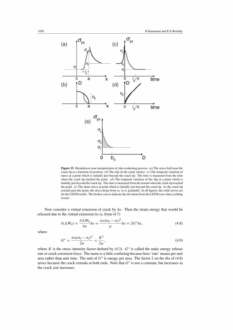
In the simple model described in figure 14 (called the linear elastic fracture model(LEFM)), the stress near the crack tip becomes indefinitely large (solid curve in figure 14(inset)). In the real material this does not occur. Instead, inelastic (e.g. plastic) yieldingoccurs, and the stress becomes finite as shown by the broken curve in figure 15(a). The finitestress at the crack tip, σY, is called the yield stress. Because of this breakdown process, thestress just inside the crack does not drop to the constant frictional level σf abruptly. Instead itdecreases gradually to σf over a distance l0 as shown by the broken curve in figure 15(a). Also,slip, D, inside the crack increases gradually to the value, D0, expected for the case withoutinelastic breakdown (i.e. LEFM), as shown in figure 15(b).
At a point just beyond the crack tip, the stress and slip vary as a function of time as shownin figures 15(c) and (d), respectively. Figure 15(e) shows the shear stress σyz at this pointas a function of slip D, as the crack tip passes by. The stress drops from σY to the constantfrictional stress σf over a slip D0. This behaviour in which the stress on the fault planedecreases as slip increases is called slip-weakening behaviour, and this model is often referredto as the breakdown-zone slip-weakening model. (For the development of the concept, seeDugdale (1960), Barenblatt (1962), Palmer and Rice (1973), Ida (1972), and for more detaileddiscussions, see Rice (1980), Li (1987).)
4.1.3. Stability and growth of a crack. Now that we have an overview of crack physics, wecan consider the stability of a crack and its growth. The theory is based on Griffith’s (1920)concept which was initially developed for tensional cracks (Mode I). Here, we use the basicconcept, and apply it to seismological problems. More details are given by Lawn (1993).
Consider a Mode III crack with half-length, a, as discussed earlier. When a crack withhalf-length a is inserted in a homogeneous medium under uniform shear stress σ0, the strainenergy is released. After subtracting the energy dissipated in friction, we obtain the energygiven by (4.6)
W0 = (σ0 − σf)DS
2= πa2(σ0 − σf)
2
2µ, (4.7)
which is available for mechanical work for crack extension.
1458 H Kanamori and E E Brodsky
Figure 15. Breakdown-zone interpretation of slip-weakening process. (a) The stress field near thecrack tip as a function of position. (b) The slip on the crack surface. (c) The temporal variation ofstress at a point which is initially just beyond the crack tip. The time is measured from the timewhen the crack tip reached the point. (d) The temporal variation of the slip at a point which isinitially just beyond the crack tip. The time is measured from the instant when the crack tip reachedthe point. (e) The shear stress at point which is initially just beyond the crack tip. As the crack tipextends past this point, the stress drops from σY to σf gradually. In all figures, the solid curves arefor the LEFM model. The broken curves indicate the deviation from the LEFM case when yieldingoccurs.
Now consider a virtual extension of crack by δa. Then the strain energy that would bereleased due to the virtual extension δa is, from (4.7)
δ(W0) = ∂W0
∂aδa = πa(σ0 − σf)
2
µδa = 2G∗δa, (4.8)
where
G∗ = πa(σ0 − σf)2
2µ= K2
2µ, (4.9)
where K is the stress intensity factor defined by (4.3). G∗ is called the static energy releaserate or crack extension force. The name is a little confusing because here ‘rate’ means per unitarea rather than unit time. The unit of G∗ is energy per area. The factor 2 on the rhs of (4.8)arises because the crack extends at both ends. Note that G∗ is not a constant, but increases asthe crack size increases.
The physics of earthquakes 1459
Static crack. In case of a static (or quasi-static) crack, for the crack to be stable at half-length a, this energy must be equal to twice the surface energy of the material near the cracktip. That is,
G∗ = G∗c ≡ 2γ, (4.10)
where γ is the surface energy per unit area which is necessary to create a new crack surface.The factor 2 in (4.10) arises because surface energy is defined for each side of the crack. If G∗
given by (4.9) is larger than G∗c , the crack will grow. G∗
c is called the critical specific fractureenergy. The stress intensity factor at this state, Kc, is called the fracture toughness (or criticalstress intensity factor), which is related to G∗
c by equation (4.9), i.e.
G∗c = K2
c
2µ. (4.11)
Thus, the stability of a crack can be discussed either in term of the critical specific fractureenergy, G∗
c , or the critical stress intensity factor, Kc.In seismic faulting, we often generalize γ to include more surface area (e.g. damaged
zones) than just the normal area of crack extension, as is done in the Griffith theory.K and G∗ are the important parameters in crack theory. The expressions for K are
independent of the mode of crack. The expression for G∗ is the same for Modes I and II, but isslightly different for Mode III, but considering the gross approximations used in seismologicalapplications, the differences are not important.
Dynamic crack. When G∗ > G∗c the crack propagates dynamically and some energy is
radiated out of the system as seismic waves. The total energy available for work fromequation (4.7) is divided between the virtual crack extension and the radiated energy. Ifwe denote the radiated energy by ER, the energy equation for virtual crack extension is nolonger given by (4.8). Instead,
δ(W0) − δ(ER) = 2Gδa, (4.12)
from which
G = G∗ − 1
2
∂ER
∂a, (4.13)
where G is called the dynamic energy release rate. Then, the crack extension is governed by
G = 2γ (4.14)
instead of (4.10).
Rupture speed. The ratio of the dynamic energy release rate, G, to the static energy releaserate, G∗, is given by a function of rupture speed V = da/dt . Kostrov (1966), Eshelby (1969)and Freund (1972) showed that the energy release rate, G, for a crack growing at a rupturespeed V is given approximately by
G = G∗g(V ), (4.15)
where g(V ) is a universal function of V .For a Mode I (tensile) crack (Freund 1972)
g(V ) = 1 − V
cR, (4.16)
where cR is the Rayleigh-wave speed.
1460 H Kanamori and E E Brodsky
For a Mode II (longitudinal shear) crack (Fossum and Freund 1975)
g(V ) = 1 − V/cR√1 − V/β
, (4.17)
where β is the shear-wave speed.For a Mode III (transverse shear) crack (Kostrov 1966, Eshelby 1969).
g(V ) =√
1 − (V/β)
1 + (V/β). (4.18)
The derivation of g(V ) given above is actually complicated, but the classical Mott’s (1948)theory is useful for understanding the basic physics. In Mott’s theory, the radiated energy ER
is equated to the kinetic energy in the medium during rupture propagation and scales as
ER ∝ a2u2 ∝ a2
(∂u
∂a
)2
a2 ∝ a2
(∂u
∂a
)2
V 2,
where u is the displacement. Because the strain energy, W0, also scales as a2 (4.7), ER canbe written as
ER = 1
B2
(V
β
)2
W0, (4.19)
where B is a constant of the order of 1 (Lawn 1993, chapter 4; Mott 1948, Marder andFineberg 1996). Then, including the kinetic energy, the equation corresponding to (4.12) canbe written as,
δ(W0) − δER =[
1 − 1
B2
(V
β
)2]
δ(W0) = 2Gδa (4.20)
from which
G = G∗g(V ), (4.21)
where
g(V ) = 1 − V 2
(Bβ)2. (4.22)
Equation (4.22) has a similar form to relativistic contraction as used to calculate theelectromagnetic field around a particle as it approaches the speed of light. Like theelectromagnetic case, acoustic waves also experience a relativistic effect because informationcan only propagate through a finite distance in a finite time.
The equation for dynamic crack extension is given from (4.14) as
G∗g(V ) = 2γ. (4.23)
In the limit of the rupture speed approaching the shear sound speed β, no energy isdissipated mechanically for a Mode III crack and all the energy is radiated in elastic waves.Modes I and II cracks display the same phenomenon at different limiting velocities. In thelimit of very small rupture speed, the relativistic contraction is irrelevant and g(V ) approachesunity.
4.2. Frictional sliding
Fault rupture can also be modelled as a frictional process. As two surfaces slide past each otheralong a pre-existing fault, the dynamics can be dominated by the surface forces between thetwo sides. Below, we quantify this frictional interaction in a way that is parallel to the cracktheory so that we can combine the two formulations in section 4.3.
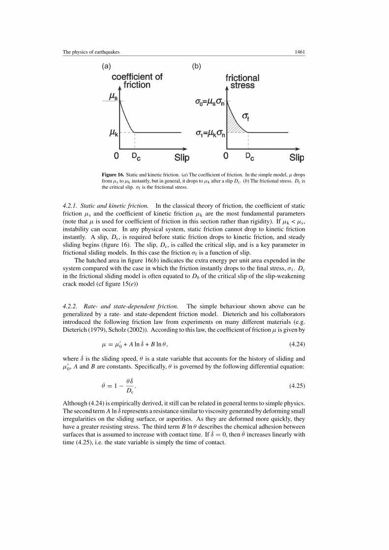
The physics of earthquakes 1461
(a) (b)
Figure 16. Static and kinetic friction. (a) The coefficient of friction. In the simple model, µ dropsfrom µs to µk instantly, but in general, it drops to µk after a slip Dc. (b) The frictional stress. Dc isthe critical slip. σf is the frictional stress.
4.2.1. Static and kinetic friction. In the classical theory of friction, the coefficient of staticfriction µs and the coefficient of kinetic friction µk are the most fundamental parameters(note that µ is used for coefficient of friction in this section rather than rigidity). If µk < µs,instability can occur. In any physical system, static friction cannot drop to kinetic frictioninstantly. A slip, Dc, is required before static friction drops to kinetic friction, and steadysliding begins (figure 16). The slip, Dc, is called the critical slip, and is a key parameter infrictional sliding models. In this case the friction σf is a function of slip.
The hatched area in figure 16(b) indicates the extra energy per unit area expended in thesystem compared with the case in which the friction instantly drops to the final stress, σ1. Dc
in the frictional sliding model is often equated to D0 of the critical slip of the slip-weakeningcrack model (cf figure 15(e))
4.2.2. Rate- and state-dependent friction. The simple behaviour shown above can begeneralized by a rate- and state-dependent friction model. Dieterich and his collaboratorsintroduced the following friction law from experiments on many different materials (e.g.Dieterich (1979), Scholz (2002)). According to this law, the coefficient of friction µ is given by
µ = µ′0 + A ln δ + B ln θ, (4.24)
where δ is the sliding speed, θ is a state variable that accounts for the history of sliding andµ′
0, A and B are constants. Specifically, θ is governed by the following differential equation:
θ = 1 − θ δ
Dc. (4.25)
Although (4.24) is empirically derived, it still can be related in general terms to simple physics.The second term A ln δ represents a resistance similar to viscosity generated by deforming smallirregularities on the sliding surface, or asperities. As they are deformed more quickly, theyhave a greater resisting stress. The third term B ln θ describes the chemical adhesion betweensurfaces that is assumed to increase with contact time. If δ = 0, then θ increases linearly withtime (4.25), i.e. the state variable is simply the time of contact.
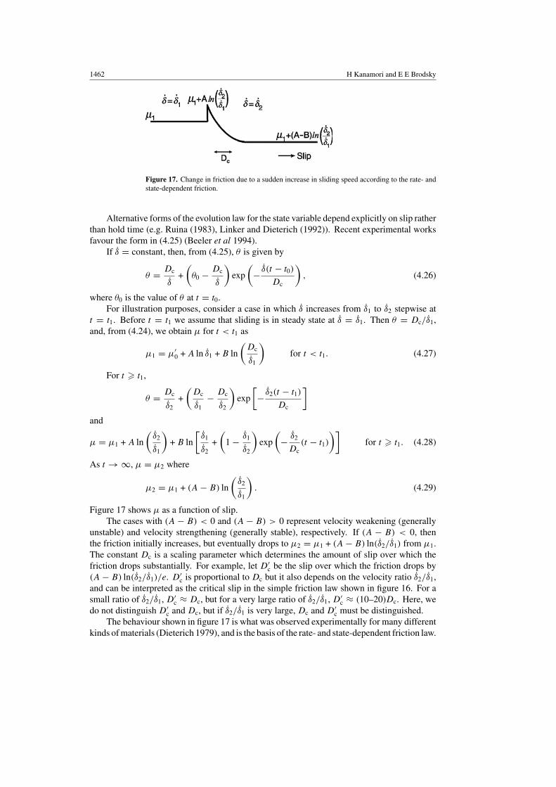
1462 H Kanamori and E E Brodsky
Figure 17. Change in friction due to a sudden increase in sliding speed according to the rate- andstate-dependent friction.
Alternative forms of the evolution law for the state variable depend explicitly on slip ratherthan hold time (e.g. Ruina (1983), Linker and Dieterich (1992)). Recent experimental worksfavour the form in (4.25) (Beeler et al 1994).
If δ = constant, then, from (4.25), θ is given by
θ = Dc
δ+
(θ0 − Dc
δ
)exp
(− δ(t − t0)
Dc
), (4.26)
where θ0 is the value of θ at t = t0.For illustration purposes, consider a case in which δ increases from δ1 to δ2 stepwise at
t = t1. Before t = t1 we assume that sliding is in steady state at δ = δ1. Then θ = Dc/δ1,and, from (4.24), we obtain µ for t < t1 as
µ1 = µ′0 + A ln δ1 + B ln
(Dc
δ1
)for t < t1. (4.27)
For t � t1,
θ = Dc
δ2+
(Dc
δ1− Dc
δ2
)exp
[− δ2(t − t1)
Dc
]
and
µ = µ1 + A ln
(δ2
δ1
)+ B ln
[δ1
δ2+
(1 − δ1
δ2
)exp
(− δ2
Dc(t − t1)
)]for t � t1. (4.28)
As t → ∞, µ = µ2 where
µ2 = µ1 + (A − B) ln
(δ2
δ1
). (4.29)
Figure 17 shows µ as a function of slip.The cases with (A − B) < 0 and (A − B) > 0 represent velocity weakening (generally
unstable) and velocity strengthening (generally stable), respectively. If (A − B) < 0, thenthe friction initially increases, but eventually drops to µ2 = µ1 + (A − B) ln(δ2/δ1) from µ1.The constant Dc is a scaling parameter which determines the amount of slip over which thefriction drops substantially. For example, let D′
c be the slip over which the friction drops by(A − B) ln(δ2/δ1)/e. D′
c is proportional to Dc but it also depends on the velocity ratio δ2/δ1,and can be interpreted as the critical slip in the simple friction law shown in figure 16. For asmall ratio of δ2/δ1, D′
c ≈ Dc, but for a very large ratio of δ2/δ1, D′c ≈ (10–20)Dc. Here, we
do not distinguish D′c and Dc, but if δ2/δ1 is very large, Dc and D′
c must be distinguished.The behaviour shown in figure 17 is what was observed experimentally for many different
kinds of materials (Dieterich 1979), and is the basis of the rate- and state-dependent friction law.
The physics of earthquakes 1463
4.3. The link between the crack model and the friction model
Crack and frictional sliding models are frequently used in seismology to explain various aspectsof earthquake phenomena. Sometimes the terminology of crack mechanics is used and at othertimes the terminology of friction mechanics is used. We need to link these two models tounderstand the way these models are used in seismology.
The fracture energy, Gc, in crack theory is the energy needed to create new crack surfacesnear the crack tip. Thus, the system must expend the threshold fracture energy Gc before thecrack can extend. In contrast, in frictional sliding model, Dc, is introduced as a critical slipbefore rapid sliding begins at a constant friction. The final value of the frictional stress σf
is equal to σ1. If the frictional stress varies more or less linearly as shown in figure 16, theenergy spent in the system before this happens can be approximately written as (hatched areain figure 16(b))
12 (σ0 − σ1)Dc. (4.30)
Thus, if we are to link a crack model to a friction model, we can equate equation (4.30) toGc, i.e.
Gc = 12 (σ0 − σ1)Dc. (4.31)
Past the initial breakdown-zone, σf is the same in the crack and friction models.
Direct determination of Dc. With the recent availability of high-quality seismograms at shortdistances, it is now possible to determine a bound on Dc directly from seismograms (Ide andTakeo 1997). With inversion of seismic data, the slip at a point on the fault plane, u(t), canbe determined as a function of time. Then solving the equation of elastodynamics on the faultplane, we can determine the shear stress, σ(t) as a function of time. Eliminating t from u(t)
and σ(t) leads to the slip dependence of stress σ(u) from which Dc can be estimated. For the1995 Kobe earthquake, Ide and Takeo (1997) found Dc to be of the order of 0.5 m in the deeperpart of the fault plane. However, in the process of inversion low-pass filtering is applied to thedata, which tends to smooth the resulting σ(u) versus u relationship. Thus, the critical slip,Dc, thus determined is an upper bound. Mikumo et al (2003) developed a method to estimateDc directly from slip-velocity records using elastodynamic modelling. With this method, Dc
for large earthquakes is also estimated to be of the order of 1 m.The values of Dc determined by laboratory friction experiments (equation (4.28)) are
approximately 5 orders of magnitude less than the upper bound derived from seismic studies.Therefore, we conclude that either the seismically determined bound on Dc is so extremethat comparison with the laboratory values is not meaningful, or the slip-weakening processat large slips is different from that of laboratory friction process. For example, Marone andKilgore (1933) suggest that Dc is controlled by the thickness of fault gouge layers as well as thesurface roughness. Ohnaka and Shen (1999) proposed a scaling relation between Dc and thewavelength of the surface roughness. Alternative slip-weakening processes include thermalpressurization, hydrodynamic lubrication (as discussed in section 4.5), plastic deformation andmicro-fracturing in the crust surrounding the fault.
4.4. Rupture energy budget
Since the crack and frictional processes are linked through the fracture energy Gc, we can relatethe macroscopically observable energy budget to the microscopic processes in a surprisinglygeneral way. Any constraint on fracture energy obtained from the energy budget will providea strong bound on all microscopic rupture processes.
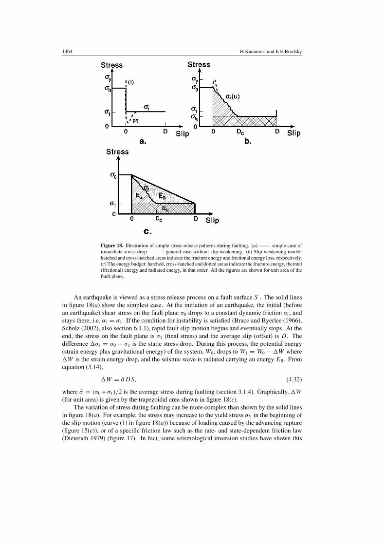
1464 H Kanamori and E E Brodsky
Figure 18. Illustration of simple stress release patterns during faulting. (a) ——: simple case ofimmediate stress drop. - - - -: general case without slip-weakening. (b) Slip-weakening model:hatched and cross-hatched areas indicate the fracture energy and frictional energy loss, respectively.(c) The energy budget: hatched, cross-hatched and dotted areas indicate the fracture energy, thermal(frictional) energy and radiated energy, in that order. All the figures are shown for unit area of thefault plane.
An earthquake is viewed as a stress release process on a fault surface S . The solid linesin figure 18(a) show the simplest case. At the initiation of an earthquake, the initial (beforean earthquake) shear stress on the fault plane σ0 drops to a constant dynamic friction σf , andstays there, i.e. σf = σ1. If the condition for instability is satisfied (Brace and Byerlee (1966),Scholz (2002), also section 6.1.1), rapid fault slip motion begins and eventually stops. At theend, the stress on the fault plane is σ1 (final stress) and the average slip (offset) is D. Thedifference σs = σ0 − σ1 is the static stress drop. During this process, the potential energy(strain energy plus gravitational energy) of the system, W0, drops to W1 = W0 − W whereW is the strain energy drop, and the seismic wave is radiated carrying an energy ER. Fromequation (3.14),
W = σDS, (4.32)
where σ = (σ0 + σ1)/2 is the average stress during faulting (section 3.1.4). Graphically, W
(for unit area) is given by the trapezoidal area shown in figure 18(c).The variation of stress during faulting can be more complex than shown by the solid lines
in figure 18(a). For example, the stress may increase to the yield stress σY in the beginning ofthe slip motion (curve (1) in figure 18(a)) because of loading caused by the advancing rupture(figure 15(e)), or of a specific friction law such as the rate- and state-dependent friction law(Dieterich 1979) (figure 17). In fact, some seismological inversion studies have shown this
The physics of earthquakes 1465
increase (Quin 1990, Miyatake 1992, Mikumo and Miyatake 1993, Beroza and Mikumo 1996,Bouchon 1997, Ide and Takeo 1997). The stress difference, σY − σ0, is called the strengthexcess. However, the amount of slip during this high stress stage is small so that little energyis involved. Thus, we will not include it in our simple energy budget.
Also, the friction may not be constant during faulting. For instance, the friction maydrop drastically in the beginning and later resumes a somewhat larger value (curve (2) infigure 18(a)), or it may decrease gradually to a constant level (figure 18(b)). As discussedbefore, this behaviour in which the stress on the fault plane gradually decreases as slipincreases is often called slip-weakening (Rice 1980, Li 1987). Slip-weakening models havebeen considered in seismological models by Brune (1970), Kikuchi and Fukao (1988), Heaton(1990) and Kikuchi (1992).
If friction is not constant, the rupture dynamics is complicated, but for the energy budgetconsidered here, we formulate this problem referring to a simple case shown in figure 18(b).The friction σf gradually drops to a constant value σf0 until the slip becomes Dc. (For simplicity,here we assume that the final stress σ1 is equal to σf0.) Then, we define the average frictionσf by
σf = 1
D
∫ D
0σf(u) du, (4.33)
where u is the slip (offset) on the fault plane. Then, the total energy dissipation is given by
S
∫ D
0σf(u) du = σfDS. (4.34)
Figure 18(c) shows the partition of energy. The area under the trapezoid outlined by the heavylines represents the total potential energy change, W . The area under the curve labelled asσf is the total dissipated energy. Then, the radiated energy, ER, is the dotted area. Thus,
ER = W − σfDS. (4.35)
As we discussed earlier, if we use the slip-weakening model, the hatched area in figure 18(c)is the fracture energy, EG. Then, the total dissipated energy σfDS can be divided into EG, andthe frictional energy, EH, represented by the cross-hatched area in figure 18(c). We shouldnote that this partition is model dependent; nevertheless it is based on the breakdown-zoneinterpretation of the slip-weakening behaviour and is useful for interpretation of the energybudget.
From figure 18(c), we obtain
ER = σ0 − σ1
2DS − EG = σs
2DS − EG = σs
2µM0 − EG, (4.36)
where M0 = µDS is the seismic moment.The ratio,
ηR = ER
ER + EG(4.37)
is called the radiation efficiency and is an important parameter which determines the dynamiccharacter of an earthquake (Husseini 1977). The radiation efficiency, ηR, is different fromthe seismic efficiency, η, which is given by ER/W . As discussed in section 3.1.4, W
cannot be determined directly by seismological methods and the seismic efficiency is difficultto determine. Because W � ER +EG, ηR � η. If ηR ≈ 1, the breakdown zone is unimportantand failure occurs primarily in the steady-state regime regardless of whether it is crack-likeor friction-dominated. On the other hand, if ηR � 1, the microscopic breakdown process isdominating the dynamics.
1466 H Kanamori and E E Brodsky
By combining (4.36) and (4.37), we obtain a relation between ηR and observableseismological parameters:
ηR = 2µ
σse, (4.38)
where
e = ER
M0(4.39)
is the radiated energy scaled by the seismic moment, i.e. scaled energy. As shown in figure 12,e is always less than 10−4, and values of e for small earthquakes are often 1–2 orders ofmagnitude less than those for large earthquakes. Whether the trend shown in figure 12 is realor not is currently debated (Ide and Beroza 2001). If it is real, for typical values of staticstress drops, 1–10 MPa, and a shear modulus, 3 × 10⁴ MPa, ηR for small earthquakes mustbe significantly less than unity. The small values of ηR for small earthquakes motivate us toexamine the micro-mechanisms of slip-weakening and breakdown.
4.5. Fault-zone processes: melting, fluid pressurization and lubrication
Motivated by the importance of the non-elastic slip-weakening processes in the energy balance,we now turn to the micromechanics of rupture beyond solid friction and crack models.
Melting. One of the first such special mechanisms recognized was frictionally-inducedmelting. As first suggested by Jeffreys (1942), frictional dissipation may be high enough,early in the rupture, to melt the wallrock. The silicate melt then reduces the friction for theremainder of the earthquake. Studies by McKenzie and Brune (1972), Richards (1976) andCardwell et al (1978) quantitatively confirmed the potential importance of frictional heatingduring faulting.
Here, we consider a gross thermal budget during faulting under a frictional stress σf . Let Sand D be the fault area and the displacement offset, respectively. Then the total heat generatedduring faulting is Q = σfDS. If we assume that the heat is distributed during seismic faultingwithin a layer of thickness w around the rupture plane and there is negligible heat transportaway over the timescale of the earthquake, the average temperature rise T is given by
T = Q
CρSw= σfD
Cρw, (4.40)
where C is the specific heat and ρ is the density. In general D increases with the earthquakemagnitude, Mw. Using the scaling relations given in section 3.2.1, we can relate D to Mw
(with the static stress drop σs as a parameter), and compute T as a function of magnitudewith three parameters, σf , w and the static stress drop σs. Figure 19 shows T for the casewith w = 1 cm as a function of Mw.
If σf is comparable to σs about 10 MPa, the effect of shear heating is significant. If thethermal energy is contained within a few centimetres around the slip plane during seismic slip,the temperature can easily rise by 100–1000˚C during a moderate-sized earthquake.
Thermal fluid pressurization. Geological outcrops of faults suggest that many faults are filledwith aqueous fluids or a viscous mixture of gouge and water when active. If this is true, thenanother set of mechanisms are at work during rupture. One possibility is thermal pressurizationof the fluid. This concept was introduced to seismology by Sibson (1973), and analysed in greatdetail by Lachenbruch (1980), Mase and Smith (1985, 1987) and Andrews (2002). Under the

The physics of earthquakes 1467
10-1
100
101
102
103
104
105
106
107
108
1 2 3 4 5 6 7 8 9 10
∆s s=10 MPa, w=1 cm
∆ T,
degr
ee
s f=1 GPa
100
101 MPa
σs
σf
Mw
Figure 19. Predicted temperature rise, T , in a fault zone as a function of magnitude, Mw, withthe frictional stress, σf , as a parameter. The static stress drop σs is assumed to be 10 MPa.
pressure–temperature conditions at the seismogenic depths, the thermal expansivity of water isof the order of 10−3˚C−1, and significant increase in pore pressure with temperature could occur.If the fluid does not escape (small permeability) and the surrounding rock is not compressible,the pressure increase would be of the order of 1 MPa per ˚C (Lachenbruch 1980). In actual faultzones, permeability and compressibility vary and the pressure increase may be less. The mostimportant parameter controlling the pressure change is the permeability. The analysis ofLachenbruch (1980) and Mase and Smith (1985, 1987) suggests that if permeability is lessthan 10−18 m2, fluid pressurization is most likely to occur with a temperature rise of less than200˚C, and the friction will drop significantly. Permeability in the crust varies over a very widerange of more than a factor of 1010. Although the distribution of permeability can be complex,these studies suggest that fluid pressurization can play an important role, at least locally, inreducing friction. A modest T of 100–200˚C would likely increase the pore pressure enoughto significantly reduce friction. Figure 19 shows that this moderate temperature increase canoccur even for intermediate-sized earthquakes (Mw = 3–5).
The key question is: what is the thickness w of the fault slip zone? Geologists haveexamined many old fault zones which were formed at depths and were brought to the surfaceby long-term uplift (i.e. exhumed faults). Some fault zones have a very narrow (about 1 mm)distinct slip zone where fault slips seem to have occurred repeatedly. According to Chesterand Chester (1998), the internal structure of the Punchbowl fault, California, implies thatearthquake ruptures were not only confined to a layer of finely shattered rock, but also largelylocalized to a thin prominent fracture surface. They suggest that mechanisms that are consistentwith the extreme localization of slip, such as thermal pressurization of pore fluids, are mostcompatible with their observations. In other cases, several narrow slip zones were found butevidence shows that each slip zone represents a distinct slip event (i.e. an earthquake). Thus,geological evidence suggests a narrow slip zone, at least for some faults, but this questionremains debatable (Sibson 2003).
1468 H Kanamori and E E Brodsky
Lubrication. If a fault zone is narrow and slightly rough, and if the material in the faultzone behaves as a viscous fluid, it is also possible that elastohydrodynamic lubrication playsan important role in reducing friction for large events (Brodsky and Kanamori 2001). As ina ball bearing, the transverse shear gradients in the fluid are balanced by the longitudinalpressure gradients and the pressure increases on the leading edge of irregularities in the faultsurface. An interesting consequence of this is that as the slip and slip velocity increase,the hydrodynamic pressure within a narrow zone becomes large enough to smooth out theirregularities on the fault surface by elastic deformation, thereby suppressing high-frequencyground motion caused by the fault surfaces rubbing against each other. During the 1999Chi-Chi, Taiwan, earthquake, the observed ground-motion near the northern end of the faultwas extremely large (>3.5 m s−1, the largest ever recorded), but short period acceleration wasnot particularly strong and the shaking damage was not the worst (Ma et al 1999). This couldbe a manifestation of the high-speed lubrication effects (Ma et al 2003). However, since this isthe only earthquake for which such large slip and slip velocity were instrumentally observed,whether this is indeed a general behaviour or not is yet to be seen.
Any of these dynamic weakening mechanisms can explain the lack of elevated heat flowover seismogenic faults (section 2.2). There is some evidence that the heat flow is slightlyelevated over the section of the San Andreas fault that slips gradually with no large earthquakes(Sass et al 1997). A high heat flow over the aseismic section would be consistent with dynamicweakening reducing the frictional dissipation where there are earthquakes.
Since a fault zone is probably complex and heterogeneous in stress, fluid content,permeability, porosity and compressibility, no single process is likely to dominate. In otherwords, we do not necessarily expect a single continuous layer of melting and pressurization;we envision, instead, a fault zone that consists of many regions where different mechanismsare responsible for slip at different stress levels, producing complex rupture patterns asobserved.
In these discussions, the thickness of fault slip zones is the key parameter for understandingfault dynamics. Of course, whether lubrication occurs or not depends on many factors suchas the effective permeability in the fault zone, compressibility of fault rocks and the viscosityof melts; but in view of the large slip and slip velocity associated with seismic faulting, asignificant drop in friction is likely to occur if the slip zone is narrow.
4.6. Linking processes to the seismic data
4.6.1. The interpretation of macroscopic seismological parametersRadiation efficiency. As we discussed in section 4.4, in the breakdown-zone interpretationof the slip-weakening model, the energy defined by the cross-hatched area in figure 18(c) isinterpreted as frictional thermal energy, EH, and is subtracted from the total potential energy; itdoes not directly control the dynamics of earthquake rupture. In contrast, the fracture energy,EG, represents the mechanical energy loss during faulting, and controls the fault dynamics ina fundamental way. Thus, the determination of fracture energy for earthquakes is criticallyimportant for understanding the dynamics of faulting. Since the radiation efficiency, ηR, isdirectly related to EG by (4.37), first we describe how we can determine ηR from macroscopicseismic parameters (Venkataraman and Kanamori 2004).
As shown by equation (4.38), we can estimate the radiation efficiency, ηR, using the threemacroscopic seismological parameters, M0, ER and σs. If ηR = 1, no energy is dissipatedmechanically and the potential energy, after heat loss has been subtracted, is radiated as seismicwaves and the earthquake is considered a very ‘brittle’ event. In contrast, if ηR = 0, the eventis quasi-static and no energy is radiated, even if the static stress drop is very large.
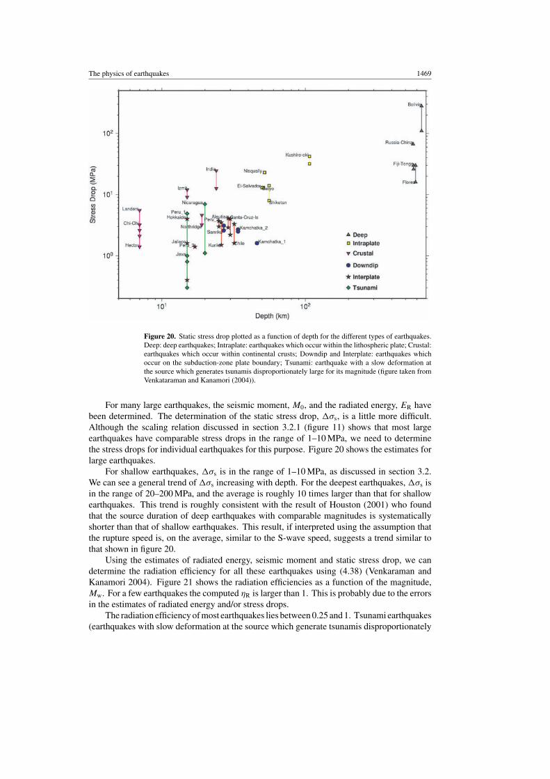
The physics of earthquakes 1469
Figure 20. Static stress drop plotted as a function of depth for the different types of earthquakes.Deep: deep earthquakes; Intraplate: earthquakes which occur within the lithospheric plate; Crustal:earthquakes which occur within continental crusts; Downdip and Interplate: earthquakes whichoccur on the subduction-zone plate boundary; Tsunami: earthquake with a slow deformation atthe source which generates tsunamis disproportionately large for its magnitude (figure taken fromVenkataraman and Kanamori (2004)).
For many large earthquakes, the seismic moment, M0, and the radiated energy, ER havebeen determined. The determination of the static stress drop, σs, is a little more difficult.Although the scaling relation discussed in section 3.2.1 (figure 11) shows that most largeearthquakes have comparable stress drops in the range of 1–10 MPa, we need to determinethe stress drops for individual earthquakes for this purpose. Figure 20 shows the estimates forlarge earthquakes.
For shallow earthquakes, σs is in the range of 1–10 MPa, as discussed in section 3.2.We can see a general trend of σs increasing with depth. For the deepest earthquakes, σs isin the range of 20–200 MPa, and the average is roughly 10 times larger than that for shallowearthquakes. This trend is roughly consistent with the result of Houston (2001) who foundthat the source duration of deep earthquakes with comparable magnitudes is systematicallyshorter than that of shallow earthquakes. This result, if interpreted using the assumption thatthe rupture speed is, on the average, similar to the S-wave speed, suggests a trend similar tothat shown in figure 20.
Using the estimates of radiated energy, seismic moment and static stress drop, we candetermine the radiation efficiency for all these earthquakes using (4.38) (Venkaraman andKanamori 2004). Figure 21 shows the radiation efficiencies as a function of the magnitude,Mw. For a few earthquakes the computed ηR is larger than 1. This is probably due to the errorsin the estimates of radiated energy and/or stress drops.
The radiation efficiency of most earthquakes lies between 0.25 and 1. Tsunami earthquakes(earthquakes with slow deformation at the source which generate tsunamis disproportionately
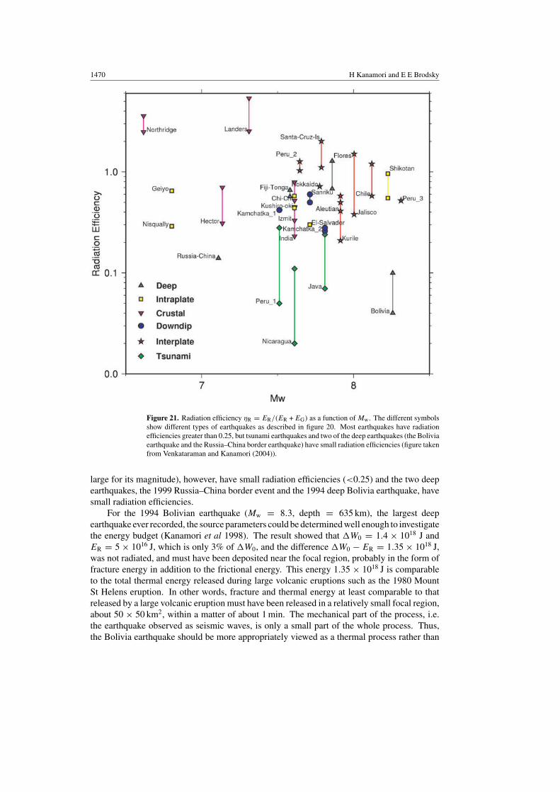
1470 H Kanamori and E E Brodsky
Figure 21. Radiation efficiency ηR = ER/(ER + EG) as a function of Mw. The different symbolsshow different types of earthquakes as described in figure 20. Most earthquakes have radiationefficiencies greater than 0.25, but tsunami earthquakes and two of the deep earthquakes (the Boliviaearthquake and the Russia–China border earthquake) have small radiation efficiencies (figure takenfrom Venkataraman and Kanamori (2004)).
large for its magnitude), however, have small radiation efficiencies (<0.25) and the two deepearthquakes, the 1999 Russia–China border event and the 1994 deep Bolivia earthquake, havesmall radiation efficiencies.
For the 1994 Bolivian earthquake (Mw = 8.3, depth = 635 km), the largest deepearthquake ever recorded, the source parameters could be determined well enough to investigatethe energy budget (Kanamori et al 1998). The result showed that W0 = 1.4 × 10¹⁸ J andER = 5 × 10¹⁶ J, which is only 3% of W0, and the difference W0 − ER = 1.35 × 10¹⁸ J,was not radiated, and must have been deposited near the focal region, probably in the form offracture energy in addition to the frictional energy. This energy 1.35 × 10¹⁸ J is comparableto the total thermal energy released during large volcanic eruptions such as the 1980 MountSt Helens eruption. In other words, fracture and thermal energy at least comparable to thatreleased by a large volcanic eruption must have been released in a relatively small focal region,about 50 × 50 km2, within a matter of about 1 min. The mechanical part of the process, i.e.the earthquake observed as seismic waves, is only a small part of the whole process. Thus,the Bolivia earthquake should be more appropriately viewed as a thermal process rather than
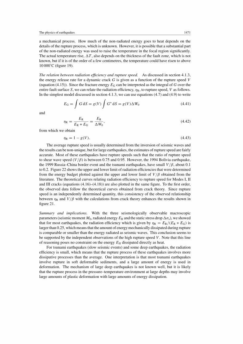
The physics of earthquakes 1471
a mechanical process. How much of the non-radiated energy goes to heat depends on thedetails of the rupture process, which is unknown. However, it is possible that a substantial partof the non-radiated energy was used to raise the temperature in the focal region significantly.The actual temperature rise, T , also depends on the thickness of the fault zone, which is notknown, but if it is of the order of a few centimetres, the temperature could have risen to above10 000˚C (figure 19).
The relation between radiation efficiency and rupture speed. As discussed in section 4.1.3,the energy release rate for a dynamic crack G is given as a function of the rupture speed V
(equation (4.15)). Since the fracture energy EG can be interpreted as the integral of G over theentire fault surface S, we can relate the radiation efficiency, ηR, to rupture speed, V as follows.In the simplest model discussed in section 4.1.3, we can use equations (4.7) and (4.9) to write
EG =∫
G dS = g(V )
∫G∗ dS = g(V )W0 (4.41)
and
ηR = ER
ER + EG= ER
W0, (4.42)
from which we obtain
ηR = 1 − g(V ). (4.43)
The average rupture speed is usually determined from the inversion of seismic waves andthe results can be non-unique, but for large earthquakes, the estimates of rupture speed are fairlyaccurate. Most of these earthquakes have rupture speeds such that the ratio of rupture speedto shear wave speed (V/β) is between 0.75 and 0.95. However, the 1994 Bolivia earthquake,the 1999 Russia–China border event and the tsunami earthquakes, have small V/β, about 0.1to 0.2. Figure 22 shows the upper and lower limit of radiation efficiencies that were determinedfrom the energy budget plotted against the upper and lower limit of V/β obtained from theliterature. The theoretical curves relating radiation efficiency to rupture speed for Modes I, IIand III cracks (equations (4.16)–(4.18)) are also plotted in the same figure. To the first order,the observed data follow the theoretical curves obtained from crack theory. Since rupturespeed is an independently determined quantity, this consistency of the observed relationshipbetween ηR and V/β with the calculations from crack theory enhances the results shown infigure 21.
Summary and implications. With the three seismologically observable macroscopicparameters (seismic moment M0, radiated energy ER and the static stress drop σs), we showedthat for most earthquakes, the radiation efficiency which is given by ηR = ER/(ER + EG) islarger than 0.25, which means that the amount of energy mechanically dissipated during ruptureis comparable or smaller than the energy radiated as seismic waves. This conclusion seems tobe supported by the independent observations of the high rupture speed V . Note that this lineof reasoning poses no constraint on the energy EH dissipated directly as heat.
For tsunami earthquakes (slow seismic events) and some deep earthquakes, the radiationefficiency is small, which means that the rupture process of these earthquakes involves moredissipative processes than the average. One interpretation is that most tsunami earthquakesinvolve rupture in soft deformable sediments, and a large amount of energy is used indeformation. The mechanism of large deep earthquakes is not known well, but it is likelythat the rupture process in the pressure–temperature environment at large depths may involvelarge amounts of plastic deformation with large amounts of energy dissipation.
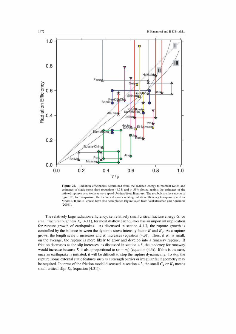
1472 H Kanamori and E E Brodsky
V / �
Figure 22. Radiation efficiencies determined from the radiated energy-to-moment ratios andestimates of static stress drop (equations (4.38) and (4.39)) plotted against the estimates of theratio of rupture speed to shear wave speed obtained from literature. The symbols are the same as infigure 20; for comparison, the theoretical curves relating radiation efficiency to rupture speed forModes I, II and III cracks have also been plotted (figure taken from Venkataraman and Kanamori(2004)).
The relatively large radiation efficiency, i.e. relatively small critical fracture energy Gc orsmall fracture toughness Kc (4.11), for most shallow earthquakes has an important implicationfor rupture growth of earthquakes. As discussed in section 4.1.3, the rupture growth iscontrolled by the balance between the dynamic stress intensity factor K and Kc. As a rupturegrows, the length scale a increases and K increases (equation (4.3)). Thus, if Kc is small,on the average, the rupture is more likely to grow and develop into a runaway rupture. Iffriction decreases as the slip increases, as discussed in section 4.5, the tendency for runawaywould increase because K is also proportional to (σ − σf) (equation (4.3)). If this is the case,once an earthquake is initiated, it will be difficult to stop the rupture dynamically. To stop therupture, some external static features such as a strength barrier or irregular fault geometry maybe required. In terms of the friction model discussed in section 4.3, the small Gc or Kc meanssmall critical slip, Dc (equation (4.31)).
The physics of earthquakes 1473
10-1
100
101
102
103
104
105
3 4 5 6 7 8 9
N(M
)
Magnitude, M
Figure 23. Magnitude–frequency relationship for earthquakes in the world for the period 1904 to1980. N(M) is the number of earthquakes per year with the magnitude �M . The solid line showsa slope of −1 on the semilog plot which corresponds to a b-value of 1. Note that, on the average,approximately one earthquake with M � 8 occurs every year. The data sources are as follows:M � 8, for the period 1904 to 1980 from Kanamori (1983); M = 5.5, 6.0, 6.5, 7.0 and 7.5, forthe period from 1976 to 2000 from Ekstrom (2000); M = 4 and 5, for the period January 1995 toJanuary 2000 from the catalogue of the Council of National Seismic System. For this range, thecatalogue may not be complete, and N may be slightly underestimated.
At present, the accuracy of the macroscopic source parameters, especially ER and σs,is not good enough to accurately estimate the fracture parameters Gc, Kc and Dc, and to drawmore definitive conclusions on the rupture dynamics of earthquakes. Currently, extensiveefforts are being made to improve the accuracy of determinations of the macroscopic sourceparameters.
5. Earthquakes as a complex system
Another possible approach to understanding why earthquakes happen is to take a broadview beyond a single event. We can study earthquakes by dealing with large groups ofearthquakes statistically. The goal is to find systems that robustly reproduce the generalpatterns of seismicity regardless of the details of the rupture microphysics. This approach hashad considerable success characterizing the types of models that will reproduce the observedmagnitude–frequency relationship (i.e. Gutenberg–Richter relation) used in seismology.
The magnitude–frequency relationship (the Gutenberg–Richter relation). In general smallearthquakes are more frequent than large earthquakes. This is quantitatively stated by theGutenberg–Richter relation (Gutenberg and Richter (1941), a recent review is found in Utsu(2002).) It describes the number of earthquakes expected of each size, or magnitude, in a givenarea. In any area much larger than the rupture area of the largest earthquake considered, thenumber of earthquakes, N(M), which have a magnitude greater than or equal to M is givenby the relation
log N(M) = a − bM, (5.1)
where a and b are constants. Figure 23 shows that the Gutenberg–Richter relationshipeven applies to a seismicity catalogue encompassing the entire planet. Approximatelyone earthquake with M � 8 occurs every year somewhere in the Earth.
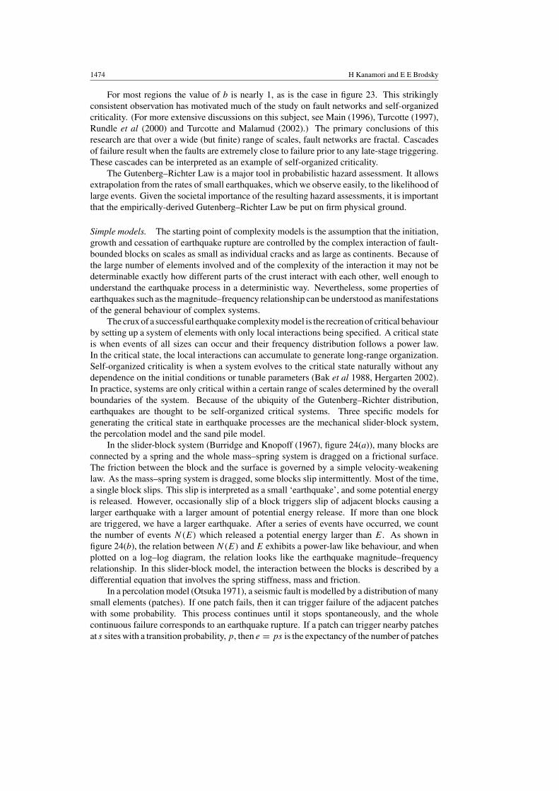
1474 H Kanamori and E E Brodsky
For most regions the value of b is nearly 1, as is the case in figure 23. This strikinglyconsistent observation has motivated much of the study on fault networks and self-organizedcriticality. (For more extensive discussions on this subject, see Main (1996), Turcotte (1997),Rundle et al (2000) and Turcotte and Malamud (2002).) The primary conclusions of thisresearch are that over a wide (but finite) range of scales, fault networks are fractal. Cascadesof failure result when the faults are extremely close to failure prior to any late-stage triggering.These cascades can be interpreted as an example of self-organized criticality.
The Gutenberg–Richter Law is a major tool in probabilistic hazard assessment. It allowsextrapolation from the rates of small earthquakes, which we observe easily, to the likelihood oflarge events. Given the societal importance of the resulting hazard assessments, it is importantthat the empirically-derived Gutenberg–Richter Law be put on firm physical ground.
Simple models. The starting point of complexity models is the assumption that the initiation,growth and cessation of earthquake rupture are controlled by the complex interaction of fault-bounded blocks on scales as small as individual cracks and as large as continents. Because ofthe large number of elements involved and of the complexity of the interaction it may not bedeterminable exactly how different parts of the crust interact with each other, well enough tounderstand the earthquake process in a deterministic way. Nevertheless, some properties ofearthquakes such as the magnitude–frequency relationship can be understood as manifestationsof the general behaviour of complex systems.
The crux of a successful earthquake complexity model is the recreation of critical behaviourby setting up a system of elements with only local interactions being specified. A critical stateis when events of all sizes can occur and their frequency distribution follows a power law.In the critical state, the local interactions can accumulate to generate long-range organization.Self-organized criticality is when a system evolves to the critical state naturally without anydependence on the initial conditions or tunable parameters (Bak et al 1988, Hergarten 2002).In practice, systems are only critical within a certain range of scales determined by the overallboundaries of the system. Because of the ubiquity of the Gutenberg–Richter distribution,earthquakes are thought to be self-organized critical systems. Three specific models forgenerating the critical state in earthquake processes are the mechanical slider-block system,the percolation model and the sand pile model.
In the slider-block system (Burridge and Knopoff (1967), figure 24(a)), many blocks areconnected by a spring and the whole mass–spring system is dragged on a frictional surface.The friction between the block and the surface is governed by a simple velocity-weakeninglaw. As the mass–spring system is dragged, some blocks slip intermittently. Most of the time,a single block slips. This slip is interpreted as a small ‘earthquake’, and some potential energyis released. However, occasionally slip of a block triggers slip of adjacent blocks causing alarger earthquake with a larger amount of potential energy release. If more than one blockare triggered, we have a larger earthquake. After a series of events have occurred, we countthe number of events N(E) which released a potential energy larger than E. As shown infigure 24(b), the relation between N(E) and E exhibits a power-law like behaviour, and whenplotted on a log–log diagram, the relation looks like the earthquake magnitude–frequencyrelationship. In this slider-block model, the interaction between the blocks is described by adifferential equation that involves the spring stiffness, mass and friction.
In a percolation model (Otsuka 1971), a seismic fault is modelled by a distribution of manysmall elements (patches). If one patch fails, then it can trigger failure of the adjacent patcheswith some probability. This process continues until it stops spontaneously, and the wholecontinuous failure corresponds to an earthquake rupture. If a patch can trigger nearby patchesat s sites with a transition probability, p, then e = ps is the expectancy of the number of patches
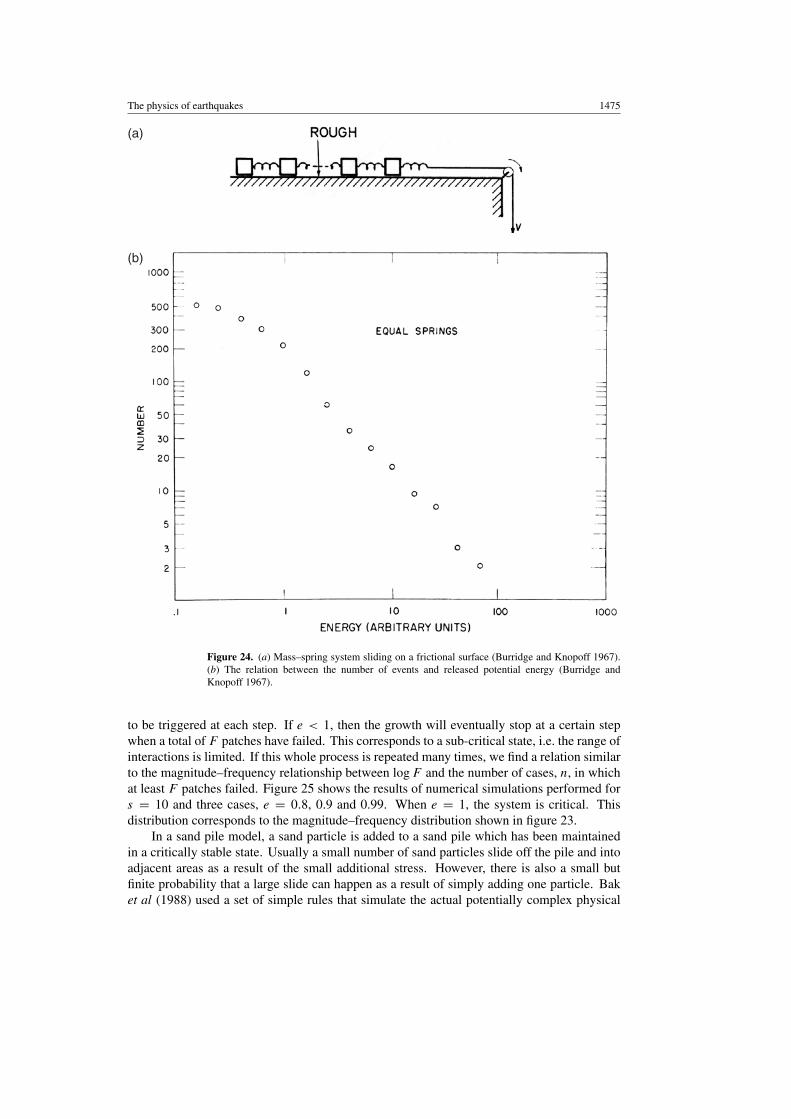
The physics of earthquakes 1475
(a)
(b)
Figure 24. (a) Mass–spring system sliding on a frictional surface (Burridge and Knopoff 1967).(b) The relation between the number of events and released potential energy (Burridge andKnopoff 1967).
to be triggered at each step. If e < 1, then the growth will eventually stop at a certain stepwhen a total of F patches have failed. This corresponds to a sub-critical state, i.e. the range ofinteractions is limited. If this whole process is repeated many times, we find a relation similarto the magnitude–frequency relationship between log F and the number of cases, n, in whichat least F patches failed. Figure 25 shows the results of numerical simulations performed fors = 10 and three cases, e = 0.8, 0.9 and 0.99. When e = 1, the system is critical. Thisdistribution corresponds to the magnitude–frequency distribution shown in figure 23.
In a sand pile model, a sand particle is added to a sand pile which has been maintainedin a critically stable state. Usually a small number of sand particles slide off the pile and intoadjacent areas as a result of the small additional stress. However, there is also a small butfinite probability that a large slide can happen as a result of simply adding one particle. Baket al (1988) used a set of simple rules that simulate the actual potentially complex physical
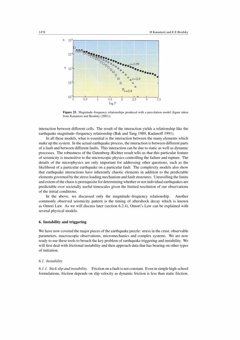
1476 H Kanamori and E E Brodsky
Figure 25. Magnitude–frequency relationships produced with a percolation model (figure takenfrom Kanamori and Brodsky (2001)).
interaction between different cells. The result of the interaction yields a relationship like theearthquake magnitude–frequency relationship (Bak and Tang 1989, Kadanoff 1991).
In all these models, what is essential is the interaction between the many elements whichmake up the system. In the actual earthquake process, the interaction is between different partsof a fault and between different faults. This interaction can be due to static as well as dynamicprocesses. The robustness of the Gutenberg–Richter result tells us that this particular featureof seismicity is insensitive to the microscopic physics controlling the failure and rupture. Thedetails of the microphysics are only important for addressing other questions, such as thelikelihood of a particular earthquake on a particular fault. The complexity models also showthat earthquake interactions have inherently chaotic elements in addition to the predictableelements governed by the stress loading mechanism and fault structures. Unravelling the limitsand extent of the chaos is prerequisite for determining whether or not individual earthquakes arepredictable over societally useful timescales given the limited resolution of our observationsof the initial conditions.
In the above, we discussed only the magnitude–frequency relationship. Anothercommonly observed seismicity pattern is the timing of aftershock decay which is knownas Omori Law. As we will discuss later (section 6.2.4), Omori’s Law can be explained withseveral physical models.
6. Instability and triggering
We have now covered the major pieces of the earthquake puzzle: stress in the crust, observableparameters, macroscopic observations, micromechanics and complex systems. We are nowready to use these tools to broach the key problem of earthquake triggering and instability. Wewill first deal with frictional instability and then approach data that has bearing on other typesof initiation.
6.1. Instability
6.1.1. Stick slip and instability. Friction on a fault is not constant. Even in simple high-schoolformulations, friction depends on slip velocity as dynamic friction is less than static friction.
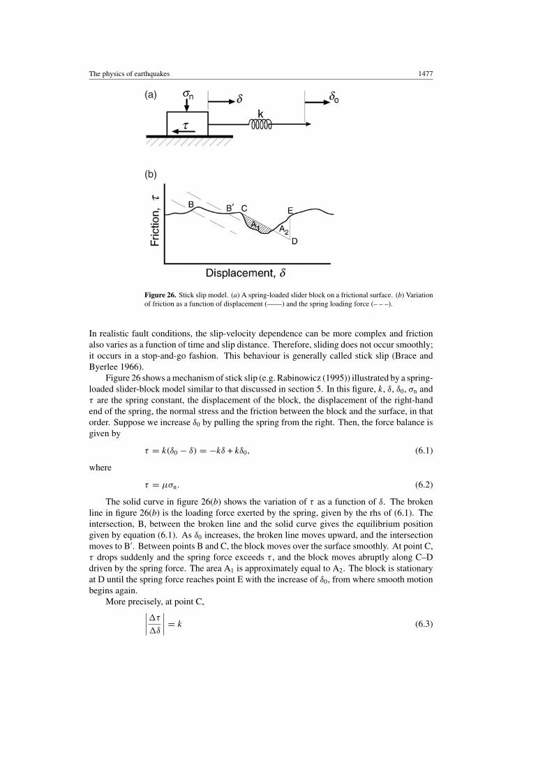
The physics of earthquakes 1477
(a)
(b)
Figure 26. Stick slip model. (a) A spring-loaded slider block on a frictional surface. (b) Variationof friction as a function of displacement (——) and the spring loading force (– – –).
In realistic fault conditions, the slip-velocity dependence can be more complex and frictionalso varies as a function of time and slip distance. Therefore, sliding does not occur smoothly;it occurs in a stop-and-go fashion. This behaviour is generally called stick slip (Brace andByerlee 1966).
Figure 26 shows a mechanism of stick slip (e.g. Rabinowicz (1995)) illustrated by a spring-loaded slider-block model similar to that discussed in section 5. In this figure, k, δ, δ0, σn andτ are the spring constant, the displacement of the block, the displacement of the right-handend of the spring, the normal stress and the friction between the block and the surface, in thatorder. Suppose we increase δ0 by pulling the spring from the right. Then, the force balance isgiven by
τ = k(δ0 − δ) = −kδ + kδ0, (6.1)
where
τ = µσn. (6.2)
The solid curve in figure 26(b) shows the variation of τ as a function of δ. The brokenline in figure 26(b) is the loading force exerted by the spring, given by the rhs of (6.1). Theintersection, B, between the broken line and the solid curve gives the equilibrium positiongiven by equation (6.1). As δ0 increases, the broken line moves upward, and the intersectionmoves to B′. Between points B and C, the block moves over the surface smoothly. At point C,τ drops suddenly and the spring force exceeds τ , and the block moves abruptly along C–Ddriven by the spring force. The area A1 is approximately equal to A2. The block is stationaryat D until the spring force reaches point E with the increase of δ0, from where smooth motionbegins again.
More precisely, at point C,∣∣∣∣τ
δ
∣∣∣∣ = k (6.3)
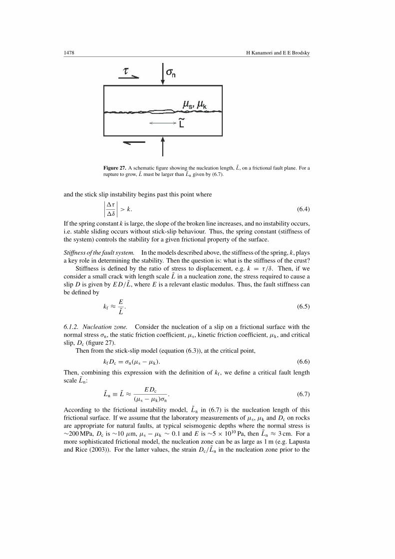
1478 H Kanamori and E E Brodsky
Figure 27. A schematic figure showing the nucleation length, L, on a frictional fault plane. For arupture to grow, L must be larger than Ln given by (6.7).
and the stick slip instability begins past this point where∣∣∣∣τ
δ
∣∣∣∣ > k. (6.4)
If the spring constant k is large, the slope of the broken line increases, and no instability occurs,i.e. stable sliding occurs without stick-slip behaviour. Thus, the spring constant (stiffness ofthe system) controls the stability for a given frictional property of the surface.
Stiffness of the fault system. In the models described above, the stiffness of the spring, k, playsa key role in determining the stability. Then the question is: what is the stiffness of the crust?
Stiffness is defined by the ratio of stress to displacement, e.g. k = τ/δ. Then, if weconsider a small crack with length scale L in a nucleation zone, the stress required to cause aslip D is given by ED/L, where E is a relevant elastic modulus. Thus, the fault stiffness canbe defined by
kf ≈ E
L. (6.5)
6.1.2. Nucleation zone. Consider the nucleation of a slip on a frictional surface with thenormal stress σn, the static friction coefficient, µs, kinetic friction coefficient, µk, and criticalslip, Dc (figure 27).
Then from the stick-slip model (equation (6.3)), at the critical point,
kfDc = σn(µs − µk). (6.6)
Then, combining this expression with the definition of kf , we define a critical fault lengthscale Ln:
Ln ≡ L ≈ EDc
(µs − µk)σn. (6.7)
According to the frictional instability model, Ln in (6.7) is the nucleation length of thisfrictional surface. If we assume that the laboratory measurements of µs, µk and Dc on rocksare appropriate for natural faults, at typical seismogenic depths where the normal stress is∼200 MPa, Dc is ∼10 µm, µs − µk ∼ 0.1 and E is ∼5 × 10¹⁰ Pa, then Ln ≈ 3 cm. For amore sophisticated frictional model, the nucleation zone can be as large as 1 m (e.g. Lapustaand Rice (2003)). For the latter values, the strain Dc/Ln in the nucleation zone prior to the
The physics of earthquakes 1479
earthquake is of the order 10−5. This relatively large strain could potentially be observed upto ∼80 m away on modern strain metres. The major impediment to testing such a predictionmethod is the very small size of the proposed nucleation zone. A geophysicist would haveto be very lucky to choose to put an instrument within 80 m of the right 1 m2 patch of the15 000 km2 San Andreas fault!
The nucleation length model in (6.7) suggests that the smallest possible earthquakes havemagnitudes Mw = −1 (from equation (3.7). Mw = −1 corresponds to M0 = 4 × 10⁷ N m).Smaller earthquakes have been observed, although they are difficult to detect. Dense networksdesigned to capture extremely small earthquakes could help confirm or refute the nucleationlength model by determining whether any lower bounds on earthquake size exists. Ifthe observation of very small earthquakes with Mw � −1 is supported, then, either theextrapolation of laboratory parameters from metre-scale samples to kilometre-scale faults isproblematic, or earthquake initiation involves other processes than simple frictional instabilityas formulated here. Another strategy for studying earthquake initiation is to examine caseswhere the immediate trigger of a real earthquake is known.
6.2. Triggering
During the past decade, seismologists have discovered that earthquakes commonly triggerother earthquakes both in the near-field and at distances approaching 4000 km (Hill et al 2002).As one of the few cases in nature where the immediate cause of an earthquake is apparent,triggering provides a fundamental clue into initiation. Observed cases of triggering are usuallyseparated into near-field (<2–3 fault lengths) and far-field, with a different set of mechanismsoperating in each regime. This distinction may be artificial, as the far-field mechanism mustalso operate in the near-field, however, it is useful in order to separate plausible regimes forcertain physics. Therefore, we will retain the separation here with the above caveats.
6.2.1. Observations. Large earthquakes are followed by abundant smaller earthquakes calledaftershocks (section 6.2.4). Aftershocks are, therefore, the most commonly observed form ofearthquake interactions. Aftershocks form a cloud around the mainshock rupture plane thatcan extend up to two fault lengths away. Beginning in the early 1990s, studies such as thoseby King et al (1994) investigated the proposal that aftershocks are triggered by the static stresschanges due to the dislocation of the earthquake. As discussed in section 3.1, the deformationof the crust by a slip on a fault plane generates an elastic strain field surrounding the fault.In some areas the strain is extensional, in others it is compressional. The pattern of dilatationalstrain can most easily be seen for the simple example of a strike-slip fault (figure 28, right).
In addition to the dilatational strain, there is also a deviatoric stress component to the stressfield. It is a combination of the shear and normal stress that will determine if a given faultplane slips. Following the Anderson, Hubbert and Rubey failure criterion laid out in section 2,we define the Coulomb stress change τc on a fault by
τc = −µ(σn − p) + τ, (6.8)
where σn and τ are the resolved normal and shear stress changes, respectively, on a givenfault orientation, p is the pore pressure change and µ is the coefficient of friction. If τc
increases, then frictional fault slip is promoted (see equation (2.6)). The King et al strategy forstudying aftershocks is to map the calculated Coulomb stress change based on the observed slipduring an earthquake and compare the resulting field with the observed aftershock distribution(figure 28).

1480 H Kanamori and E E Brodsky
Figure 28. Change in Coulomb stress from the 1979 Homestead Valley mainshock and thesubsequent aftershocks. Red (positive) indicates that optimally oriented faults are stressed moretowards failure and purple (negative) indicates that failure is inhibited. White circles are observedaftershocks (from King et al (1994)). Shown on the right is a schematic of a strike-slip fault withslip in the directions shown by the arrows. The dilatational strain is compressional where there are‘+’ signs and extensional where there are ‘−’ signs.
This method has had some success in predicting the location of aftershocks and even afew large, nearby earthquakes (Stein 1999). Approximately 85% of the aftershocks of the1992 Mw = 7.3 Landers earthquake occurred where the Coulomb stress field increased atthe time of the mainshock (Hardebeck et al 1998). A recent review can be found in Harris(2002).
Equation (6.8) by itself does not fully describe the aftershock field shown in figure 28.There are some aftershocks in the areas where failure should have been inhibited by themainshock. This problem of a continual low aftershock rate in the destressed regions wasaddressed by adding rate- and state-dependent friction (section 4.2.2) to the stress transfermodel (Stein et al 2003). Dieterich (1994) showed that if velocity and memory-dependenceare incorporated into the standard frictional coefficient based on laboratory experiments, thenthe rate of seismicity, rather than the absolute number of events, will be influenced by a stressstep. Therefore, we might expect some aftershocks to occur in all areas of the stress field ifthe background seismicity rate is fairly high, but the aftershock rate relative to the backgroundrate will vary systematically with the imposed Coulomb stress.
Since the pattern of static Coulomb stress increase is controlled by the mainshock faultgeometry, some other mechanisms could possibly produce similar predictions. In particular, thedynamic stresses follow a very similar pattern because the strong and weak areas of shaking arealso determined by the mainshock fault geometry. One major difference between the static anddynamic stress is that only the dynamic field is affected by rupture directivity (section 3.1.5).
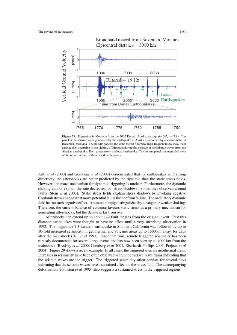
The physics of earthquakes 1481
Figure 29. Triggering in Montana from the 2002 Denali, Alaska, earthquake (Mw = 7.9). Toppanel is the seismic wave generated by the earthquake in Alaska as recorded by a seismometer inBozeman, Montana. The middle panel is the same record filtered at high-frequencies to show localearthquakes occurring in the vicinity of Montana during the passage of the seismic waves from theAlaskan earthquake. Each green arrow is a local earthquake. The bottom panel is a magnified viewof the record of one of these local earthquakes.
Kilb et al (2000) and Gomberg et al (2003) demonstrated that for earthquakes with strongdirectivity, the aftershocks are better predicted by the dynamic than the static stress fields.However, the exact mechanism for dynamic triggering is unclear. Furthermore, the dynamicshaking cannot explain the rate decreases, or ‘stress shadows’, sometimes observed aroundfaults (Stein et al 2003). Static stress fields explain stress shadows by invoking negativeCoulomb stress changes that move potential faults further from failure. The oscillatory dynamicfield has no such negative effect. Areas are simply distinguished by stronger or weaker shaking.Therefore, the current balance of evidence favours static stress as a primary mechanism forgenerating aftershocks, but the debate is far from over.
Aftershocks can extend up to about 1–2 fault lengths from the original event. Past thisdistance earthquakes were thought to have no effect until a very surprising observation in1992. The magnitude 7.3 Landers earthquake in Southern California was followed by up to10-fold increased seismicity in geothermal and volcanic areas up to 1500 km away, for daysafter the mainshock (Hill et al 1993). Since that time, remote triggered seismicity has beenrobustly documented for several large events and has now been seen up to 4000 km from themainshock (Brodsky et al 2000, Gomberg et al 2001, Eberhardt-Phillips 2003, Prejean et al2004). Figure 29 shows a recent example. In all cases, the triggered sites are geothermal areas.Increases in seismicity have been often observed within the surface wave trains indicating thatthe seismic waves are the trigger. The triggered seismicity often persists for several daysindicating that the seismic waves have a sustained effect on the stress field. The accompanyingdeformation (Johnston et al 1995) also suggests a sustained stress in the triggered regions.
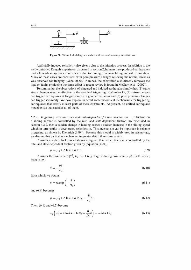
1482 H Kanamori and E E Brodsky
�0
Figure 30. Slider-block sliding on a surface with rate- and state-dependent friction.
Artificially induced seismicity also gives a clue to the initiation process. In addition to thewell-controlled Rangely experiment discussed in section 2, humans have produced earthquakesunder less advantageous circumstances due to mining, reservoir filling and oil exploitation.Many of these cases are consistent with pore pressure changes relieving the normal stress aswas observed for Rangely (Guha 2000). In mines, the excavation also directly removes theload on faults producing the same effect (a recent review is found in McGarr et al (2002)).
To summarize, the observations of triggered and induced earthquakes imply that: (1) staticstress changes may be effective in the nearfield triggering of aftershocks, (2) seismic wavescan trigger earthquakes at long-distances in geothermal areas and (3) pore pressure changescan trigger seismicity. We now explore in detail some theoretical mechanisms for triggeringearthquakes that satisfy at least parts of these constraints. At present, no unified earthquakemodel exists that satisfies all of them.
6.2.2. Triggering with the rate- and state-dependent friction mechanism. If friction ona sliding surface is controlled by the rate- and state-dependent friction law discussed insection 4.2.2, then a sudden change in loading causes a sudden increase in the sliding speedwhich in turn results in accelerated seismic slip. This mechanism can be important in seismictriggering, as shown by Dieterich (1994). Because this model is widely used in seismology,we discuss this particular mechanism in greater detail than some others.
Consider a slider-block model shown in figure 30 in which friction is controlled by therate- and state-dependent friction given by (equation (4.24))
µ = µ′0 + A ln δ + B ln θ. (6.9)
Consider the case where |θ δ/Dc| 1 (e.g. large δ during coseismic slip). In this case,from (4.25)
θ = − θ δ
Dc, (6.10)
from which we obtain
θ = θ0 exp
(− δ
Dc
)(6.11)
and (6.9) becomes
µ = µ′0 + A ln δ + B ln θ0 − B
Dcδ. (6.12)
Then, (6.1) and (6.2) become
σn
(µ′
0 + A ln δ + B ln θ0 − B
Dcδ
)= −kδ + kδ0. (6.13)
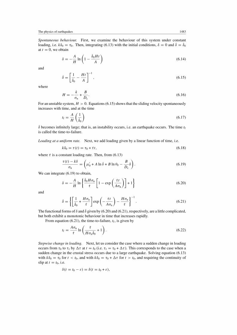
The physics of earthquakes 1483
Spontaneous behaviour. First, we examine the behaviour of this system under constantloading, i.e. kδ0 = τ0. Then, integrating (6.13) with the initial conditions, δ = 0 and δ = δ0
at t = 0, we obtain
δ = − A
Hln
(1 − δ0Ht
A
)(6.14)
and
δ =[
1
δ0− Ht
A
]−1
, (6.15)
where
H = − k
σn+
B
Dc. (6.16)
For an unstable system, H > 0. Equations (6.15) shows that the sliding velocity spontaneouslyincreases with time, and at the time
tf = A
H
(1
δ0
)(6.17)
δ becomes infinitely large; that is, an instability occurs, i.e. an earthquake occurs. The time tfis called the time-to-failure.
Loading at a uniform rate. Next, we add loading given by a linear function of time, i.e.
kδ0 = τ(t) = τ0 + τ t, (6.18)
where τ is a constant loading rate. Then, from (6.13)
τ(t) − kδ
σn=
(µ′
0 + A ln δ + B ln θ0 − B
Dcδ
). (6.19)
We can integrate (6.19) to obtain,
δ = − A
Hln
{δ0Hσn
τ
[1 − exp
(τ t
Aσn
)]+ 1
}(6.20)
and
δ ={[
1
δ0+
Hσn
τ
]exp
(− τ t
Aσn
)− Hσn
τ
}−1
. (6.21)
The functional forms of δ and δ given by (6.20) and (6.21), respectively, are a little complicated,but both exhibit a monotonic behaviour in time that increases rapidly.
From equation (6.21), the time-to-failure, tf , is given by
tf = Aσn
τln
(τ
Hσnδ0+ 1
). (6.22)
Stepwise change in loading. Next, let us consider the case where a sudden change in loadingoccurs from τ0 to τ1 by τ at t = t0 (i.e. τ1 = τ0 + τ ). This corresponds to the case when asudden change in the crustal stress occurs due to a large earthquake. Solving equation (6.13)with kδ0 = τ0 for t < t0, and with kδ0 = τ0 + τ for t > t0, and requiring the continuity ofslip at t = t0, i.e.
δ(t = t0 − ε) = δ(t = t0 + ε),
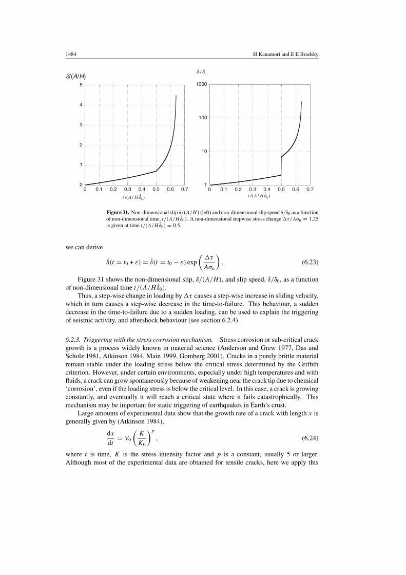
1484 H Kanamori and E E Brodsky
0
1
2
3
4
5
0 0.1 0.2 0.3 0.4 0.5 0.6 0.71
10
100
1000
0 0.1 0.2 0.3 0.4 0.5 0.6 0.7
δ/(A/H)0/δ δ
. .
0/( / )t A Hδ.
0/( / )t A Hδ.
Figure 31. Non-dimensional slip δ/(A/H) (left) and non-dimensional slip speed δ/δ0 as a functionof non-dimensional time, t/(A/H δ0). A non-dimensional stepwise stress change τ/Aσn = 1.25is given at time t/(A/H δ0) = 0.5.
we can derive
δ(t = t0 + ε) = δ(t = t0 − ε) exp
(τ
Aσn
). (6.23)
Figure 31 shows the non-dimensional slip, δ/(A/H), and slip speed, δ/δ0, as a functionof non-dimensional time t/(A/H δ0).
Thus, a step-wise change in loading by τ causes a step-wise increase in sliding velocity,which in turn causes a step-wise decrease in the time-to-failure. This behaviour, a suddendecrease in the time-to-failure due to a sudden loading, can be used to explain the triggeringof seismic activity, and aftershock behaviour (see section 6.2.4).
6.2.3. Triggering with the stress corrosion mechanism. Stress corrosion or sub-critical crackgrowth is a process widely known in material science (Anderson and Grew 1977, Das andScholz 1981, Atkinson 1984, Main 1999, Gomberg 2001). Cracks in a purely brittle materialremain stable under the loading stress below the critical stress determined by the Griffithcriterion. However, under certain environments, especially under high temperatures and withfluids, a crack can grow spontaneously because of weakening near the crack tip due to chemical‘corrosion’, even if the loading stress is below the critical level. In this case, a crack is growingconstantly, and eventually it will reach a critical state where it fails catastrophically. Thismechanism may be important for static triggering of earthquakes in Earth’s crust.
Large amounts of experimental data show that the growth rate of a crack with length x isgenerally given by (Atkinson 1984),
dx
dt= V0
(K
K0
)p
, (6.24)
where t is time, K is the stress intensity factor and p is a constant, usually 5 or larger.Although most of the experimental data are obtained for tensile cracks, here we apply this
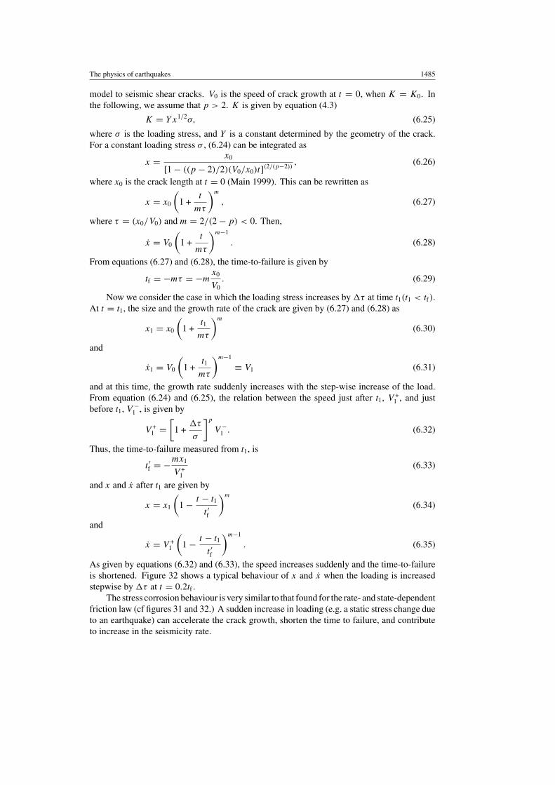
The physics of earthquakes 1485
model to seismic shear cracks. V0 is the speed of crack growth at t = 0, when K = K0. Inthe following, we assume that p > 2. K is given by equation (4.3)
K = Yx1/2σ, (6.25)
where σ is the loading stress, and Y is a constant determined by the geometry of the crack.For a constant loading stress σ , (6.24) can be integrated as
x = x0
[1 − ((p − 2)/2)(V0/x0)t](2/(p−2))
, (6.26)
where x0 is the crack length at t = 0 (Main 1999). This can be rewritten as
x = x0
(1 +
t
mτ
)m
, (6.27)
where τ = (x0/V0) and m = 2/(2 − p) < 0. Then,
x = V0
(1 +
t
mτ
)m−1
. (6.28)
From equations (6.27) and (6.28), the time-to-failure is given by
tf = −mτ = −mx0
V0. (6.29)
Now we consider the case in which the loading stress increases by τ at time t1(t1 < tf).At t = t1, the size and the growth rate of the crack are given by (6.27) and (6.28) as
x1 = x0
(1 +
t1
mτ
)m
(6.30)
and
x1 = V0
(1 +
t1
mτ
)m−1
≡ V1 (6.31)
and at this time, the growth rate suddenly increases with the step-wise increase of the load.From equation (6.24) and (6.25), the relation between the speed just after t1, V +
1 , and justbefore t1, V −
1 , is given by
V +1 =
[1 +
τ
σ
]p
V −1 . (6.32)
Thus, the time-to-failure measured from t1, is
t ′f = −mx1
V +1
(6.33)
and x and x after t1 are given by
x = x1
(1 − t − t1
t ′f
)m
(6.34)
and
x = V +1
(1 − t − t1
t ′f
)m−1
. (6.35)
As given by equations (6.32) and (6.33), the speed increases suddenly and the time-to-failureis shortened. Figure 32 shows a typical behaviour of x and x when the loading is increasedstepwise by τ at t = 0.2tf .
The stress corrosion behaviour is very similar to that found for the rate- and state-dependentfriction law (cf figures 31 and 32.) A sudden increase in loading (e.g. a static stress change dueto an earthquake) can accelerate the crack growth, shorten the time to failure, and contributeto increase in the seismicity rate.
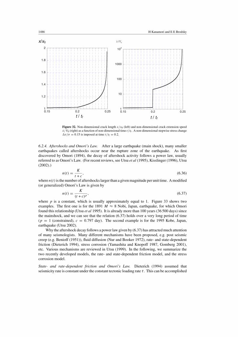
1486 H Kanamori and E E Brodsky
1
1.2
1.4
1.6
1.8
2
0.15 0.2 0.251
10
100
1000
104
0.15 0.2 0.25
x/x0 0/x V.
t / tf t / tf
Figure 32. Non-dimensional crack length x/x0 (left) and non-dimensional crack extension speedx/V0 (right) as a function of non-dimensional time t/tf . A non-dimensional stepwise stress changeτ/σ = 0.15 is imposed at time t/tf = 0.2.
6.2.4. Aftershocks and Omori’s Law. After a large earthquake (main shock), many smallerearthquakes called aftershocks occur near the rupture zone of the earthquake. As firstdiscovered by Omori (1894), the decay of aftershock activity follows a power law, usuallyreferred to as Omori’s Law. (For recent reviews, see Utsu et al (1995), Kisslinger (1996), Utsu(2002).)
n(t) = K
t + c, (6.36)
where n(t) is the number of aftershocks larger than a given magnitude per unit time. A modified(or generalized) Omori’s Law is given by
n(t) = K
(t + c)p, (6.37)
where p is a constant, which is usually approximately equal to 1. Figure 33 shows twoexamples. The first one is for the 1891 M ≈ 8 Nobi, Japan, earthquake, for which Omorifound this relationship (Utsu et al 1995). It is already more than 100 years (36 500 days) sincethe mainshock, and we can see that the relation (6.37) holds over a very long period of time(p = 1 (constrained), c = 0.797 day). The second example is for the 1995 Kobe, Japan,earthquake (Utsu 2002).
Why the aftershock decay follows a power law given by (6.37) has attracted much attentionof many seismologists. Many different mechanisms have been proposed, e.g. post seismiccreep (e.g. Benioff (1951)), fluid diffusion (Nur and Booker 1972), rate- and state-dependentfriction (Dieterich 1994), stress corrosion (Yamashita and Knopoff 1987, Gomberg 2001),etc. Various mechanisms are reviewed in Utsu (1999). In the following, we summarize thetwo recently developed models, the rate- and state-dependent friction model, and the stresscorrosion model.
State- and rate-dependent friction and Omori’s Law. Dieterich (1994) assumed thatseismicity rate is constant under the constant tectonic loading rate τ . This can be accomplished
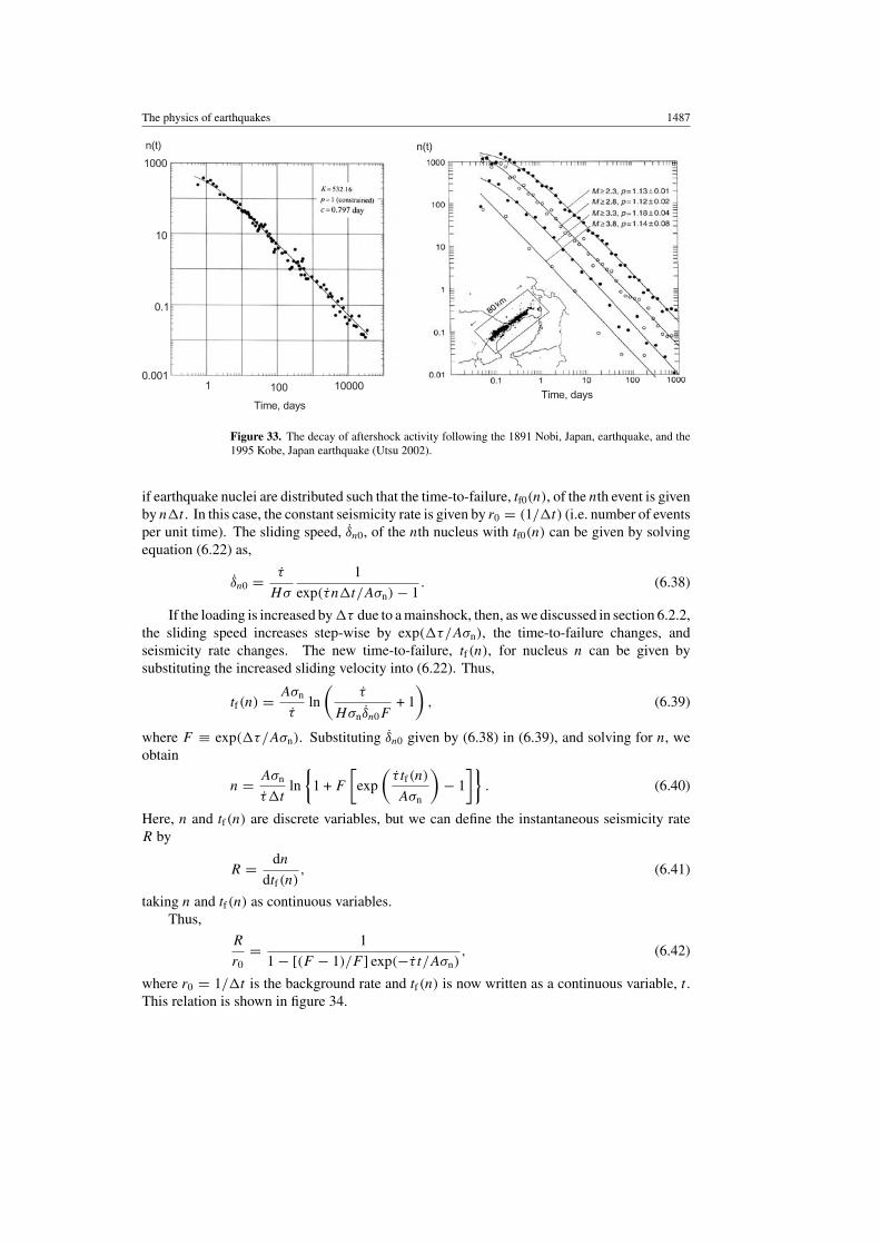
The physics of earthquakes 1487
Time, daysTime, days
n(t) n(t)
1000
10
0.1
0.0011 100 10000
Figure 33. The decay of aftershock activity following the 1891 Nobi, Japan, earthquake, and the1995 Kobe, Japan earthquake (Utsu 2002).
if earthquake nuclei are distributed such that the time-to-failure, tf0(n), of the nth event is givenby nt . In this case, the constant seismicity rate is given by r0 = (1/t) (i.e. number of eventsper unit time). The sliding speed, δn0, of the nth nucleus with tf0(n) can be given by solvingequation (6.22) as,
δn0 = τ
Hσ
1
exp(τnt/Aσn) − 1. (6.38)
If the loading is increased by τ due to a mainshock, then, as we discussed in section 6.2.2,the sliding speed increases step-wise by exp(τ/Aσn), the time-to-failure changes, andseismicity rate changes. The new time-to-failure, tf(n), for nucleus n can be given bysubstituting the increased sliding velocity into (6.22). Thus,
tf(n) = Aσn
τln
(τ
Hσnδn0F+ 1
), (6.39)
where F ≡ exp(τ/Aσn). Substituting δn0 given by (6.38) in (6.39), and solving for n, weobtain
n = Aσn
τtln
{1 + F
[exp
(τ tf(n)
Aσn
)− 1
]}. (6.40)
Here, n and tf(n) are discrete variables, but we can define the instantaneous seismicity rateR by
R = dn
dtf(n), (6.41)
taking n and tf(n) as continuous variables.Thus,
R
r0= 1
1 − [(F − 1)/F ] exp(−τ t/Aσn), (6.42)
where r0 = 1/t is the background rate and tf(n) is now written as a continuous variable, t .This relation is shown in figure 34.
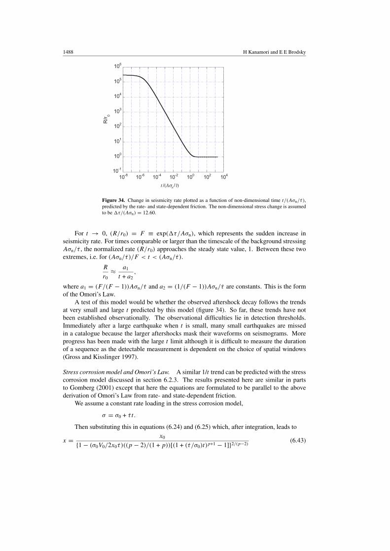
1488 H Kanamori and E E Brodsky
10-1
100
101
102
103
104
105
106
10-8 10-6 10-4 10-2 100 102 104
R/r
0
t /(A )σn/τ.
Figure 34. Change in seismicity rate plotted as a function of non-dimensional time t/(Aσn/τ ),predicted by the rate- and state-dependent friction. The non-dimensional stress change is assumedto be τ/(Aσn) = 12.60.
For t → 0, (R/r0) = F ≡ exp(τ/Aσn), which represents the sudden increase inseismicity rate. For times comparable or larger than the timescale of the background stressingAσn/τ , the normalized rate (R/r0) approaches the steady state value, 1. Between these twoextremes, i.e. for (Aσn/τ )/F < t < (Aσn/τ ).
R
r0≈ a1
t + a2,
where a1 = (F/(F − 1))Aσn/τ and a2 = (1/(F − 1))Aσn/τ are constants. This is the formof the Omori’s Law.
A test of this model would be whether the observed aftershock decay follows the trendsat very small and large t predicted by this model (figure 34). So far, these trends have notbeen established observationally. The observational difficulties lie in detection thresholds.Immediately after a large earthquake when t is small, many small earthquakes are missedin a catalogue because the larger aftershocks mask their waveforms on seismograms. Moreprogress has been made with the large t limit although it is difficult to measure the durationof a sequence as the detectable measurement is dependent on the choice of spatial windows(Gross and Kisslinger 1997).
Stress corrosion model and Omori’s Law. A similar 1/t trend can be predicted with the stresscorrosion model discussed in section 6.2.3. The results presented here are similar in partsto Gomberg (2001) except that here the equations are formulated to be parallel to the abovederivation of Omori’s Law from rate- and state-dependent friction.
We assume a constant rate loading in the stress corrosion model,
σ = σ0 + τ t .
Then substituting this in equations (6.24) and (6.25) which, after integration, leads to
x = x0
{1 − (σ0V0/2x0τ )((p − 2)/(1 + p))[(1 + (τ /σ0)t)p+1 − 1]}2/(p−2)(6.43)

The physics of earthquakes 1489
and
x = V0(1 + (τ /σ0)t)p
{1 − (σ0V0/2x0τ )((p − 2)/(1 + p))[(1 + (τ /σ0)t)p+1 − 1]}2/(p−2)+1. (6.44)
From (6.44), the time-to-failure tf can be determined as,
tf = σ0
τ
{[2x0τ (1 + p)
(p − 2)σ0V0+ 1
]1(p+1)
− 1
}. (6.45)
As discussed above, a constant seismicity rate r0 = (1/t) can be produced by distributingearthquake nuclei such that the time-to-failure, tf0(n), of nth event is given by nt . The slidingspeed, Vn0, of the nth nucleus with tf0(n) can be given by solving equation (6.45) as,
Vn0 = 2(1 + p)
p − 2
x0τ
σ0
1
((τ /σ0)nt + 1)p+1 − 1. (6.46)
If the loading is increased by τ at t = 0 due to a mainshock, then, as we discussedin section 6.2.3 with equation (6.23), the sliding speed increases step-wise by a factor ofF ≡ (1 + (τ/σ0))
p, the time-to-failure changes, and the seismicity rate changes. The newtime-to-failure, tf(n), for a nucleus n can be given by substituting the increased sliding velocity,FVn0, into (6.45). Thus,
tf(n) = σ0
τ
{[2x0τ (1 + p)
(p − 2)σ0FVn0+ 1
]1/(p+1)
− 1
}
= σ0
τ
{[1 +
((τ /σ0)nt + 1)p+1 − 1
F
]1/(p+1)
− 1
}. (6.47)
Solving this for n, we obtain
n = σ0
τt
[F
[(τ
σ0tf(n) + 1
)p+1
− 1
]+ 1
]1/(p+1)
− 1
. (6.48)
Here, n and tf(n) are discrete variables, but we can define the instantaneous seismicityrate R by
R = dn
dtf(n)(6.49)
taking n and tf(n) as continuous variables.Thus,
R
r0= F
[F + (1 − F)
(1 +
τ
σ0t
)−(p+1)]−p/(p+1)
, (6.50)
where tf(n) is now denoted simply by t . For t = 0, R/r0 = F and for t σ0/τ ,R/r0 = F 1/(p+1).
Because p is large, for t � σ0/τ , R/r0 has the form a1/((a2 + t)p/(1+p)) ≈a1/(a2 + t) which is the Omori’s law, where a1 = (F/(F − 1))(σ0/(p + 1)τ ) and a2 =(1/(F − 1))(σ0/(p + 1)τ ).
An example of a solution with typical parameters is shown in figure 35. The similarity tothe rate and state model solution in figure 34 suggests that the form of the decay in seismicitywith time is controlled by the similar mathematical construction with both cases. In both cases,the initial distribution of earthquake nuclei is designed to yield a constant rate under constantstressing rates.
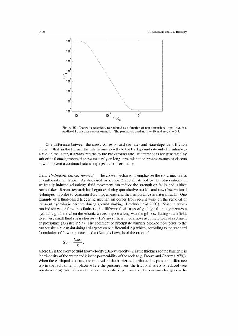
1490 H Kanamori and E E Brodsky
Figure 35. Change in seismicity rate plotted as a function of non-dimensional time t/(σ0/τ ),predicted by the stress corrosion model. The parameters used are p = 40, and τ/σ = 0.5.
One difference between the stress corrosion and the rate- and state-dependent frictionmodel is that, in the former, the rate returns exactly to the background rate only for infinite p
while, in the latter, it always returns to the background rate. If aftershocks are generated bysub-critical crack growth, then we must rely on long-term relaxation processes such as viscousflow to prevent a continual ratcheting upwards of seismicity.
6.2.5. Hydrologic barrier removal. The above mechanisms emphasize the solid mechanicsof earthquake initiation. As discussed in section 2 and illustrated by the observations ofartificially induced seismicity, fluid movement can reduce the strength on faults and initiateearthquakes. Recent research has begun exploring quantitative models and new observationaltechniques in order to constrain fluid movements and their importance in natural faults. Oneexample of a fluid-based triggering mechanism comes from recent work on the removal oftransient hydrologic barriers during ground shaking (Brodsky et al 2003). Seismic wavescan induce water flow into faults as the differential stiffness of geological units generates ahydraulic gradient when the seismic waves impose a long-wavelength, oscillating strain field.Even very small fluid shear stresses ∼1 Pa are sufficient to remove accumulations of sedimentor precipitate (Kessler 1993). The sediment or precipitate barriers blocked flow prior to theearthquake while maintaining a sharp pressure differential p which, according to the standardformulation of flow in porous media (Darcy’s Law), is of the order of
p = Udhη
k,
where Ud is the average fluid flow velocity (Darcy velocity), h is the thickness of the barrier, η isthe viscosity of the water and k is the permeability of the rock (e.g. Freeze and Cherry (1979)).When the earthquake occurs, the removal of the barrier redistributes this pressure differencep in the fault zone. In places where the pressure rises, the frictional stress is reduced (seeequation (2.6)), and failure can occur. For realistic parameters, the pressure changes can be
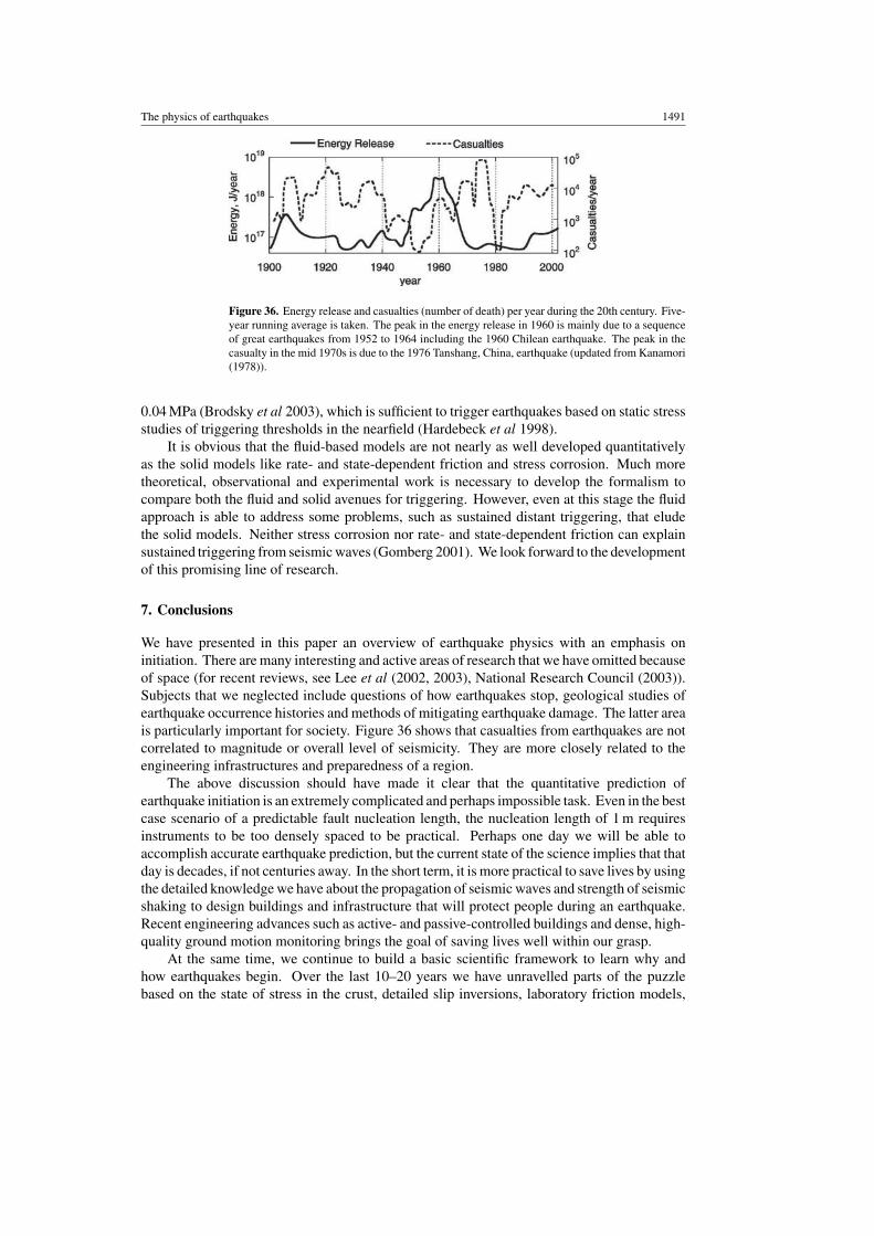
The physics of earthquakes 1491
Figure 36. Energy release and casualties (number of death) per year during the 20th century. Five-year running average is taken. The peak in the energy release in 1960 is mainly due to a sequenceof great earthquakes from 1952 to 1964 including the 1960 Chilean earthquake. The peak in thecasualty in the mid 1970s is due to the 1976 Tanshang, China, earthquake (updated from Kanamori(1978)).
0.04 MPa (Brodsky et al 2003), which is sufficient to trigger earthquakes based on static stressstudies of triggering thresholds in the nearfield (Hardebeck et al 1998).
It is obvious that the fluid-based models are not nearly as well developed quantitativelyas the solid models like rate- and state-dependent friction and stress corrosion. Much moretheoretical, observational and experimental work is necessary to develop the formalism tocompare both the fluid and solid avenues for triggering. However, even at this stage the fluidapproach is able to address some problems, such as sustained distant triggering, that eludethe solid models. Neither stress corrosion nor rate- and state-dependent friction can explainsustained triggering from seismic waves (Gomberg 2001). We look forward to the developmentof this promising line of research.
7. Conclusions
We have presented in this paper an overview of earthquake physics with an emphasis oninitiation. There are many interesting and active areas of research that we have omitted becauseof space (for recent reviews, see Lee et al (2002, 2003), National Research Council (2003)).Subjects that we neglected include questions of how earthquakes stop, geological studies ofearthquake occurrence histories and methods of mitigating earthquake damage. The latter areais particularly important for society. Figure 36 shows that casualties from earthquakes are notcorrelated to magnitude or overall level of seismicity. They are more closely related to theengineering infrastructures and preparedness of a region.
The above discussion should have made it clear that the quantitative prediction ofearthquake initiation is an extremely complicated and perhaps impossible task. Even in the bestcase scenario of a predictable fault nucleation length, the nucleation length of 1 m requiresinstruments to be too densely spaced to be practical. Perhaps one day we will be able toaccomplish accurate earthquake prediction, but the current state of the science implies that thatday is decades, if not centuries away. In the short term, it is more practical to save lives by usingthe detailed knowledge we have about the propagation of seismic waves and strength of seismicshaking to design buildings and infrastructure that will protect people during an earthquake.Recent engineering advances such as active- and passive-controlled buildings and dense, high-quality ground motion monitoring brings the goal of saving lives well within our grasp.
At the same time, we continue to build a basic scientific framework to learn why andhow earthquakes begin. Over the last 10–20 years we have unravelled parts of the puzzlebased on the state of stress in the crust, detailed slip inversions, laboratory friction models,
1492 H Kanamori and E E Brodsky
complex system modelling and triggering studies. A number of still unanswered questionsremain. Many of the questions highlighted during the course of this review will only beaddressed by improved instrumentation and observational techniques. Technical developmentslike the recently deployed dense seismic networks of Japan and the Earthscope instrumentationinitiative in the United States may help us measure seismic parameters like stress drop andradiated energy to sufficient accuracy to finally address the dynamic similarity of earthquakes.Another recent advance is the use of non-seismic data to study earthquakes. This reviewemphasized elastic waves as the most developed method for characterizing earthquakes, butinsights from geodetic methods are becoming increasingly important. As the subject expandsbeyond classic elasticity, we predict that input from geology and hydrogeology will play agreater role in the decades to come. Combining disciplines might allow us to measure migratingfluids and if their pressures can equal or exceed the minimum principal stress as suggestedby normal faulting studies. We must also grapple with the thickness and physical propertiesof the fault zone. Seismic and other observations will also have to address the heterogeneityof stress and strength in the crust. Mechanisms for triggering can be differentiated by studiestargeting phenomena where the predictions diverge. The beginning of aftershock sequences,the existence of very small earthquakes and the occurrence of long-range triggering are a fewareas with some resolving power.
Theorists and experimentalists also have their work cut out for them. Averages likethat taken in estimating the stress drop need to put on firmer theoretical ground. Theorists andexperimentalists will have to explore the relationship between initiation conditions and rupturepropagation. Is the same physics applicable or does a new set of processes come into playonce rapid slip has begun? What is the physical nature of the fracture energy term that controlsdynamics ranging from slow quasi-static slip to brittle failure with high rupture speed andefficient energy radiation? What happens when the mechanisms such as thermal pressurizationand lubrication are combined in a single rupture model? The complexity community must tryto ascertain exactly how chaotic are earthquakes. Even chaotic systems, like weather, can bepredicted over short time horizons if the observations have sufficient resolution. Quantificationof the required resolution and the divergence rate from initial conditions would be a valuablecontribution.
As our observational database improves, our computational ability accelerates and ourlaboratories become more refined, the next few decades promise to bring more earthquakeinsights and perhaps some answers.
Acknowledgments
We thank Allan Rubin and an anonymous reviewer for constructive comments.
References
Abercrombie R 1995 J. Geophys. Res. 100 24003–14Abercrombie R and Leary P 1993 Geophys. Res. Lett. 20 1511–4Aki K 1966 Bull. Earthquake Res. Inst. Tokyo Univ. 44 73–88Aki K and Richards P G 2002 Quantitative Seismology (Sausalito: University Science Books) p 685Anderson E M 1905 Trans. Edin. Geol. Soc. 8 393Anderson E M 1951 The Dynamics of Faulting and Dyke Formation with Applications to Britain (Edinburgh: Oliver
and Boyd) p 206Anderson O L and Grew P C 1977 Rev. Geophys. 15 77–104Andrews D J 2002 J. Geophys. Res. 107 (B2) 2363Atkinson B K 1984 J. Geophys. Res. 89 4077–114

The physics of earthquakes 1493
Axen G J 2004 Low-angle normal fault mechanics and crustal strength Rheology and Deformation in the Lithosphereat Continental Margins ed G Karner et al (New York: Columbia University Press) pp 46–91
Bak P and Tang C 1989 J. Geophys. Res. 94 15635–7Bak P et al 1988 Phys. Rev. A 38 364–74Barenblatt G I 1962 The mathematical theory of equilibrium cracks in brittle fracture Advances in Applied Mechanics
vol 7 (London: Academic) pp 55–125Beeler N M et al 1994 Geophys. Res. Lett. 21 1987–90Benioff H 1951 Bull. Seismol. Soc. Am. 41 31–62Beroza G C and Mikumo T 1996 J. Geophys. Res. 101 22449–60Bird P and Kagan Y Y 2004 Bull. Seismol. Soc. Am. at pressBoatwright J and Choy G L 1986 J. Geophys. Res. 91 2095–112Boatwright J et al 2002 Bull. Seismol. Soc. Am. 92 1241–55Bouchon M 1997 J. Geophys. Res. 102 11731–44Bouchon M and Vallee M 2003 Science 301 824–6Brace W F and Byerlee J D 1966 Science 153 990–2Brodsky E E and Kanamori H 2001 J. Geophys. Res. 106 16357–74Brodsky E E et al 2000 Geophys. Res. Lett. 27 2741–4Brodsky E E et al 2003 J. Geophys. Res. 108Brune J N 1970 J. Geophys. Res. 75 4997–5009Burridge R and Knopoff L 1964 Bull. Seismol. Soc. Am. 54 1875–88Burridge R and Knopoff L 1967 Bull. Seismol. Soc. Am. 57 341–71Byerlee J 1978 Pure Appl. Geophys. 116 615–26Byerlee J 1992 Tectonophysics 211 295–303Cardwell R K et al 1978 Geophys. J. R. Astron. Soc. 52 525–30Chester F M and Chester J S 1998 Tectonophysics 295 199–221Choy G L and Boatwright J L 1995 J. Geophys. Res. 100 18205–28Dahlen F A 1977 Geophys. J. R. Astron. Soc. 48 239–61Dahlen F A and Tromp J 1998 Theoretical Global Seismology (Princeton, NJ: Princeton University Press) p 1025Das S 1988 Bull. Seismol. Soc. Am. 78 924–30Das S and Scholz C H 1981 J. Geophys. Res. 86 6039–51Dieterich J 1994 J. Geophys. Res. 99 2601–18Dieterich J H 1979 J. Geophys. Res. 84 2161–8Dmowska R and Rice J R 1986 Fracture theory and its seismological applications Theories in Solid Earth Physics
ed R Teisseyre (Warzawa: PWN-Polish Publishers) pp 187–255Dragert H et al 2001 Science 292 1525–8Dugdale D S 1960 J. Mech. Phys. Solids 8 100–4Eberhart-Phillips D et al 2003 Science 300 1113–18Ekstrom E 2000 Global studies of earthquakes Problems in Geophysics for the New Millennium ed G E E Boschi and
A Morelli (Bologna: Editorice Compositori) pp 111–24Eshelby J D 1969 J. Mech. Phys. Solids 17 177–99Fossum A F and Freund L B 1975 J. Geophys. Res. 80 3343–7Freeze R A and Cherry J A 1979 Groundwater (Englewood Cliffs, NJ: Prentice Hall)Freund L B 1972 J. Elasticity 2 341–9Freund L B 1989 Dynamic Fracture Mechanics (Cambridge: Cambridge University Press) p 563Gilbert F and Dziewonski A M 1975 Phil. Trans. R. Soc. Lond. 278 187–269Gomberg J 2001 J. Geophys. Res. 106 16253–63Gomberg J et al 2001 Nature 411 462–6Gomberg J et al 2003 Bull. Seismol. Soc. Am. 93 118–38Griffith A A 1920 Phil. Trans. R. Soc. Lond. A 221 169–98Gross S and Kisslinger C 1997 J. Geophys. Res. Solid Earth 102 7603–12Guha S K 2000 Induced Earthquakes (London: Kluwer) p 314Gutenberg B and Richter C F 1941 Geol. Soc. Am. 34 1–131 (special paper)Hardebeck J L and Hauksson E 2001 J. Geophys. Res. 106 21859–82Hardebeck J L et al 1998 J. Geophys. Res. 103 24427–37Harris R A 2002 Stress triggers, stress shadows, and seismic hazard International Handbook of Earthquake &
Engineering Seismology part B, ed H Kanamori et al (San Diego, CA: Academic) pp 1217–32Haskell N 1964 Bull. Seismol. Soc. Am. 56 1811–42Heaton T 1990 Phys. Earth Planet. Inter. 64 1–20
1494 H Kanamori and E E Brodsky
Hergaten S 2002 Self-Organized Criticality in Earth Systems (Berlin: Springer) p 272Hill D P et al 2002 Phys. Today 55 41–7Hill D P et al 1993 Science 260 1617–23Houston H 2001 J. Geophys. Res. 106 11137–50Hubbert M K and Rubey W W 1959 Geol. Soc. Am. 70 115–66 (Special paper)Husseini M I 1977 Geophys. J. R. Astron. Soc. 49 699–714Ida Y 1972 J. Geophys. Res. 77 3796–805Ide S and Beroza G C 2001 Geophys. Res. Lett. 28 3349–52Ide S and Takeo M 1997 J. Geophys. Res. 102 27379–91Ikeda R et al 2001 Isl. Arc. 10 252–60Izutani Y and Kanamori H 2001 Geophys. Res. Lett. 28 4007–10Jaeger J C and Cook N G W 1979 Fundamentals of Rock Mechanics (London: Chapman and Hall) p 593Jeffreys H 1942 Geol. Mag. 79 291–5Johnston M J S et al 1995 Bull. Seismol. Soc. Am. 85 787–95Jost M L et al 1998 Bull. Seismol. Soc. Am. 88 815–32Kadanoff L P 1991 Phys. Today 44 9–10Kanamori H 1978 Nature 271 411–14Kanamori H 1983 Global seismicity Earthquakes: Observation, Theory and Interpretation ed H Kanamori and
E Boschi (New York: North-Holland) pp 596–608Kanamori H and Anderson D L 1975 Bull. Seismol. Soc. Am. 65 1073–95Kanamori H et al 1998 Science 279 839–42Kanamori H and Brodsky E E 2001 Phys. Today 54 34–40Kanamori H et al 1993 Bull. Seismol. Soc. Am. 83 330–46Kessler J H 1993 Berkeley University of California, BerkeleyKikuchi M 1992 Tectonophysics 211 107–13Kikuchi M and Fukao Y 1988 Bull. Seismol. Soc. Am. 78 1707–24Kikuchi M and Kanamori H 1994 Geophys. Res. Lett. 21 2341–4Kikuchi M and Kanamori H 1995 Pure Appl. Geophys. 144 441–53Kilb D et al 2000 Nature 408 570–4King G C P et al 1994 Bull. Seismol. Soc. Am. 84 935–53Kinoshita S and Ohike M 2002 Bull. Seismol. Soc. Am. 92 611–24Kisslinger C 1996 Aftershocks and fault-zone properties Advances in Geophysics vol 38, ed R Dmowska and
B Saltzman (San Diego, CA: Academic) pp 1–36Knopoff L 1958 Geophys. J. 1 44–52Kostrov B V 1966 J. Appl. Math. Mech. 30 1241–8 (PMM) (Engl. tans.)Kostrov B V 1974 Izv. Earth Phys. 1 23–40Lachenbruch A H 1980 J. Geophys. Res. 85 6097–112Lachenbruch A H and Sass J H 1980 J. Geophys. Res. 85 6185–222Lapusta N and Rice J R 2003 J. Geophys. Res. 108 (B4) 2205Lawn B 1993 Fracture of Brittle Solids 2nd edn (Cambridge: Cambridge University Press) p 378Lay T and Wallace T C 1995 Modern Global Seismology (San Diego, CA: Academic) p 521Lee W H K et al 2002 International Handbook of Earthquake & Engineering Seismology part A (San Diego, CA:
Academic) pp 1–933Lee W H K et al 2003 International Handbook of Earthquake & Engineering Seismology part B (San Diego, CA:
Academic) pp 937–1945Li V C 1987 Mechanics of shear rupture applied to earthquake zones Fracture Mechanics of Rock (London: Acdemic)
pp 351–428Linker M and Dieterich J H 1992 J. Geophys. Res. Solid Earth 97 4923–40Lockner D A 1995 Rock failure in rock physics & phase relations A Handbook of Physical Constants vol 3, ed T J Ahrens
(Washington, DC: American Geophysical Union) pp 127–47Lockner D A and Beeler N M 2002 Rock failure and earthquakes International Handbook of Earthquake & Engineering
Seismology part A, ed W H K Lee et al (San Diego, CA: Academic) pp 505–37Ma K F et al 2003 Geophys. Res. Lett. 30 (5) 1244Ma K-F et al 1999 EOS Trans.—AGU 80 605Madariaga R 1977 Pure Appl. Geophys. 115 301–16Madariaga R 1979 J. Geophys. Res. 84 2243–50Madariaga R and Olsen K B 2002 Earthquake dynamics International Handbook of Earthquake & Engineering
Seismology part A, ed W H K Lee et al (San Diego, CA: Academic) pp 175–94
The physics of earthquakes 1495
Main I 1996 Rev. Geophys. 34 pp 433–62Main I G 1999 Geophys. J. Int. 139 F1–6Marder M and Fineberg J 1996 Phys. Today 49 24–9Marone C and Kilgore B 1993 Nature 362 618–21Maruyama T 1964 Bull. Earthquake Res. Inst. Tokyo Univ. 42 289–368Mase C W and Smith L 1985 Pure Appl. Geophys. 122 583–607Mase C W and Smith L 1987 J. Geophys. Res. 92 6249–72Massonnet D et al 1993 Nature 364 138–42Mayeda K and Walter W R 1996 J. Geophys. Res. 101 11195–208McGarr A and Fletcher J B 2002 Bull. Seismol. Soc. Am. 92 1633–46McGarr A et al 2002 Case histories of induced and triggered seismicity International Handbook of Earthquake &
Engineering Seismology part A, ed W H K Lee et al (San Diego, CA: Academic) pp 647–61McKenzie D P and Brune J N 1972 Geophys. J. R. Astron. Soc. 29 65–78Mikumo T and Miyatake T 1993 Geophys. J. Int. 112 481–96Mikumo T et al 2003 Bull. Seismol. Soc. Am. 93 264–82Miyatake T 1992 Geophys. Res. Lett. 19 1041–4Mott N F 1948 Engineering 165 16National Research Council 2003 Living on an Active Earth (Washington, DC: National Academies) p 418Nur A and Booker J 1972 Science 175 885–7Ohnaka M and Shen L-F 1999 J. Geophys. Res. 104 817–44Omori F 1894 J. College of Science Imperial University of Tokyo 7 111–200Otsuka M 1971 J. Seismol. Soc. Japan 24 215–27Palmer A C and Rice J R 1973 Proc. R. Soc. Lond. Ser. A—Math. Phys. Eng. Sci. 332 527–48Perez-Campos X and Beroza G C 2001 J. Geophys. Res. 106 11127–36Prejean S G and Ellsworth W L 2001 Bull. Seismol. Soc. Am. 91 165–77Prejean S G et al 2004 Bull. Seismol. Soc. Am. 94 at pressProvost A S and Houston H 2003 J. Geophys. Res. 108 (B3) 2175Quin H 1990 Tectonophysics 175 93–117Rabinowicz E 1995 Friction and Wear of Materials (New York: Wiley) p 315Raleigh C B et al 1976 Science 191 1230–7Rice J R 1980 The mechanics of earthquake rupture Physics of the Earth’s Interior ed A M Dziewonski and E Boschi
(Amsterdam: North-Holland) pp 555–649Rice J R 1992 Fault stress states, pore pressure distributions, and the weakness of the San Andreas fault Fault Mechanics
and Transport Properties of Rock ed B Evans and T-F Wong (San Diego, CA: Academic) pp 475–503Richards P G 1976 Bull. Seismol. Soc. Am. 66 1–32Richardson E and Jordan T H 2002 Bull. Seismol. Soc. Am. 92 1766–82Romanowicz B and Ruff L J 2002 Geophys. Res. Lett. 29 (12) 1604Romanowicz B and Rundle J B 1993 Bull. Seismol. Soc. Am. 83 1294–7Rosakis A J 2002 Adv. Phys. 51 1189–257Rubin A M et al 1999 Nature 400 635–41Rudnicki J W and Kanamori H 1981 J. Geophys. Res. 86 1785–93Ruina A L 1983 J. Geophys. Res. 88 10359–70Rundle J B et al 2000 GeoComplexity and the Physics of Earth (Washington, DC: American Geophysical Union)
p 284Saffer D M et al 2003 J. Geophys. Res. 108 (B5) 2274Sass J H et al 1997 J. Geophys. Res. 102 27575–85Scholz C H 1994 Bull. Seismol. Soc. Am. 84 215–18Scholz C H 2002 The Mechanics of Earthquakes and Faulting (New York: Cambridge University Press) p 471Sibson R H 1973 Nature 243 66–8Sibson R H 1985 J. Struct. Geol. 7 751–4Sibson R H 2003 Bull. Seismol. Soc. Am. 93 1169–78Sibson R H and Xie G Y 1998 Bull. Seismol. Soc. Am. 88 1014–22Simons M et al 2002 Bull. Seismol. Soc. Am. 92 1390–402Singh S K et al 2004 Bull. Seismol. Soc. Am. 94 at pressStein R S 1999 Nature 402 605–9Stein R S et al 2003 Sci. Am. 288 72–9Stekette J A 1958 Can. J. Phys. 36 1168–98Tibi R et al 2003 J. Geophys. Res. 108 (B2) 2091
1496 H Kanamori and E E Brodsky
Tsuboi C 1933 Japan. J. Astron. Geophys. 10 93–248Turcotte D L 1997 Fractals and Chaos in Geology and Geophysics (Cambridge, UK: Cambridge University Press)
p 398Turcotte D L and Malamud B D 2002 Earthquakes as a complex system International Handbook of Earthquake &
Engineering Seismology part A, ed W H K Lee et al (San Diego, CA: Academic) pp 209–35Utsu T 1999 Seismicity Studies: A Comprehensive Review (Tokyo: University of Tokyo Press) p 876 (in Japanese)Utsu T 2002 Statistical features of seismicity International Handbook of Earthquake & Engineering Seismology
part A, ed W H K Lee (San Diego, CA: Academic) pp 719–32Utsu T et al 1995 J. Phys. Earth 43 1–33Uyeda S 1978 The New View of the Earth (San Francisco: W H Freeman and Company) p 217Venkataraman A and Kanamori H 2004 J. Geophys. Res. 109 B05302, 10.1029/2003JB002549Venkataraman A et al 2002 Bull. Seismol. Soc. Am. 92 1256–65Wald D J and Heaton T H 1994 Bull. Seismol. Soc. Am. 84 668–91Wernicke B 1981 Nature 291 645–8Wyss M and Brune J N 1968 J. Geophys. Res. 73 4681–94Yamashita T and Knopoff L 1987 Geophys. J. 91 13–26Zeng Y H et al 1994 Geophys. Res. Lett. 21 725–8Zoback M D and Healy J H 1984 Ann. Geophys. 2 689–98Zoback M D et al 1987 Science 238 1105–11