et discipline ou spécialité

Jury :

le

Institut Supérieur de l’Aéronautique et de l’Espace (ISAE)

Leandro RIBEIRO LUSTOSA

mardi 14 novembre 2017

La Phi-théorie : une approche pour la conception de lois de commande de voldes véhicules convertibles

The Phi-theory approach to flight control design of hybrid vehicles

ED AA : Dynamique des fluides et Robotique

Équipes d'accueil ISAE-ONERA EDyF et CSDV

Mme Caroline BERARD Professeur ISAE-SUPAERO - PrésidenteM. François DEFAY Ingénieur-Chercheur ISAE-SUPAERO - Co-directeur de thèse

M. Tarek HAMEL Professeur Université Nice Sophia Antipolis - RapporteurM. Pascal MORIN Professeur Université Pierre et Marie Curie - RapporteurM. Jean-Marc MOSCHETTA Professeur ISAE-SUPAERO - Directeur de thèse

M. Bart REMES Chercheur MAVLab TU Delft

M. Jean-Marc MOSCHETTA (directeur de thèse)M. François DEFAY (co-directeur de thèse)

Remerciements

I highly believe the readers of this particular section can be divided in three distinctflavors : (i) my family, (ii) curious colleagues, and (iii) prospective ISAE-SUPAERO PhDstudents looking for clues regarding my PhD experience. I will address you all in the following.

Regarding my family, there are no words that could be written here to reflect their supportduring this entire journey. This should come as no surprise, but a PhD thesis demands anincredible amount of tenacity. The required stamina, endurance and patience comes fromthe life-long perfect balance of (i) wise words and down-to-earth advices from my mom and(ii) inadequate jokes and let-him-jump-to-see-what-happens life guidelines from my dad andbrother.

As for my colleagues, I had the distinct privilege of working with the best (in every senseof the word and under any reasonable cost function). The road for the PhD title is filled withuncertainties and disturbances, but being surrounded by those guys helped me gain hope tocontinue, even when headwind seemed too strong to overcome. Thank you (alphabetically) :Alain, for answering my Pixhawk questions whenever needed (somehow, by chance, it wasalways Friday night) ; Caroline, for your insights into the (often upside down) academic world ;Corentin, for bringing reason every time our group started going out of control ; Daria, for ourmemorable Tomb Raider with Quantum Mechanics marathons and your remarkable quick-witted humor ; Dominique, for the many hours devoted to help me debug my drone by flyingit under stressful conditions (and yet, always joyful) ; Facundo, for stealing my Havaianasand understanding me going overboard about it ; Flavio, for our lengthy and rather unusualpaper discussions ; Igor, for sharing pizza and laughs in late-night ISAE deadline-imminentmoments ; Jan, for sticking to the bro code and being legend.. wait for it.. doctor ! ; Jessica, forher flight dynamics skills and bringing cold drinks during hot Toulouse summers ; Louis, forintegrating the Paparazzi version of the MAVion (and reintegrating it after every unsuccessfulflight until it actually flew !) ; Megan, for all our wild rides ; Nicolai, for supporting me during amajor academic failure moment involving an Uber driver ; Pascal, for your impeccable humorand teaching me how to speak like a real toulousain (he failed to teach me how to correctlypronounce pneu crevé though) ; Paulo, for using his framing effect abilities to make our dailyroutines better ; Remy and Sebastien, for sharing with me their extensive experience on windtunnel campaigns ; Sergio, for our Kalman filtering with guitar lessons ; Soheib (Birds), forour enlightening career conversations and (less enlightening) LPV control talks ; Thibault, forteaching me how to navigate effectively through French bureaucracy. If one of you guys isreading this, I hope you are laughing as much as I am.

A truly special thanks goes to my advisors, Dr. Jean-Marc Moschetta and Dr. FrançoisDefay. They carefully guided this thesis through a successful road and provided me with state-of-the-art tools to perform my research. Additionally, they provided me with outstandingprofessional opportunities and bestowed their beloved MAVion drone project on me. Theywere open to my ideas, and respectfully pointed out (more than I would like to admit) bad

i

ones. I understand prospective students might read this section looking for clues regarding myPhD experience. If that is your case, consider this thesis my written-in-stone recommendationletter for my advisors. I can’t overstate their importance in the context of this thesis. As abonus, you will fall head over heels with Toulouse, I guarantee you.

At last, I support free education for everyone, everywhere, and highly praise Prof. RussTedrake and Prof. Barton Zwiebach for their beautiful courses on underactuated robotics andquantum mechanics, respectively, at edX.org. Finally, I gratefully acknowledge the ConselhoNacional de Desenvolvimento Científico e Tecnológico, CNPq (Brazilian National ScienceFoundation), for partial financial support for this work through the Ciência sem Fronteirasprogram.

ii

Table des matières

Acronyms xiii

Abstract (English) 1

Abstract (French) 3

1 Introduction 5

1.1 A glimpse at the hybrid aerial vehicles (HAV) landscape . . . . . . . . . . . . 5

1.2 HAV modeling and control design state of the art . . . . . . . . . . . . . . . . 7

1.3 Thesis motivation . . . . . . . . . . . . . . . . . . . . . . . . . . . . . . . . . . 10

1.4 Thesis roadmap . . . . . . . . . . . . . . . . . . . . . . . . . . . . . . . . . . . 10

1.5 Notation . . . . . . . . . . . . . . . . . . . . . . . . . . . . . . . . . . . . . . . 11

Part I - An introduction to φ-theory 15

2 The φ-theory approach to wing aerodynamics modeling 17

2.1 Aerodynamic forces and moments . . . . . . . . . . . . . . . . . . . . . . . . . 17

2.2 Finite wing aerodynamic coefficients . . . . . . . . . . . . . . . . . . . . . . . 26

2.3 Wing-propeller interaction . . . . . . . . . . . . . . . . . . . . . . . . . . . . . 32

2.4 Final remarks . . . . . . . . . . . . . . . . . . . . . . . . . . . . . . . . . . . . 34

3 Transition flight modeling 35

3.1 Tilt-body physical and mathematical model . . . . . . . . . . . . . . . . . . . 35

3.2 Longitudinal flight analysis . . . . . . . . . . . . . . . . . . . . . . . . . . . . 40

3.3 Banking turn analysis . . . . . . . . . . . . . . . . . . . . . . . . . . . . . . . 47

3.4 An opportune piloting interface . . . . . . . . . . . . . . . . . . . . . . . . . . 48

iii

Part II - An autopilot design case study and flight testing 51

4 MAVion architecture overview 53

4.1 A brief history . . . . . . . . . . . . . . . . . . . . . . . . . . . . . . . . . . . 53

4.2 Physical specifications . . . . . . . . . . . . . . . . . . . . . . . . . . . . . . . 54

4.3 Avionics . . . . . . . . . . . . . . . . . . . . . . . . . . . . . . . . . . . . . . . 55

5 Control system design 57

5.1 Introduction . . . . . . . . . . . . . . . . . . . . . . . . . . . . . . . . . . . . . 57

5.2 The region-of-attraction-based gain-scheduling approach . . . . . . . . . . . . 59

5.3 The feasibility issue in RoA-GS – a case study . . . . . . . . . . . . . . . . . 62

5.4 The quaternion uncontrollable linearized dynamics conundrum . . . . . . . . 69

5.5 The MAVion control architecture . . . . . . . . . . . . . . . . . . . . . . . . . 79

5.6 Simulation investigation . . . . . . . . . . . . . . . . . . . . . . . . . . . . . . 80

5.7 Closing remarks . . . . . . . . . . . . . . . . . . . . . . . . . . . . . . . . . . . 82

6 Navigation system design 87

6.1 Introduction . . . . . . . . . . . . . . . . . . . . . . . . . . . . . . . . . . . . . 87

6.2 Avionics modeling . . . . . . . . . . . . . . . . . . . . . . . . . . . . . . . . . 89

6.3 Complementary filtering revisited . . . . . . . . . . . . . . . . . . . . . . . . . 91

6.4 The CF-EKF filter . . . . . . . . . . . . . . . . . . . . . . . . . . . . . . . . . 96

6.5 Simulation investigation . . . . . . . . . . . . . . . . . . . . . . . . . . . . . . 97

6.6 Final remarks . . . . . . . . . . . . . . . . . . . . . . . . . . . . . . . . . . . . 98

7 Flight simulation and flight testing 101

7.1 Introduction . . . . . . . . . . . . . . . . . . . . . . . . . . . . . . . . . . . . . 101

7.2 Flight simulations . . . . . . . . . . . . . . . . . . . . . . . . . . . . . . . . . 101

7.3 Flight experiments . . . . . . . . . . . . . . . . . . . . . . . . . . . . . . . . . 102

iv

7.4 Concluding remarks . . . . . . . . . . . . . . . . . . . . . . . . . . . . . . . . 103

Conclusion 109

A Falling leaf example data 111

Bibliographie 121

v

Table des figures

1.1 Commercial examples of HAVs. . . . . . . . . . . . . . . . . . . . . . . . . . . 6

2.1 The illustrated choice of body axes will be consistently followed throughoutthis thesis for airfoils and wings. Notice that b2 is such that b3 = b1 × b2. . . 18

2.2 Admissible terminal Tv geometries in view of different Φ � 0 : (i) all direc-tions are admissible since Tv configures a closed surface in R3 ; (ii) all terminalvelocities are contained in the same plane, namely, Π = ker(Φ(mv)) ; (iii) onlytwo antipodal terminal velocities are admissible ; (iv) Φ(mv) is nonsingular anddoes not admit terminal velocities. . . . . . . . . . . . . . . . . . . . . . . . . 24

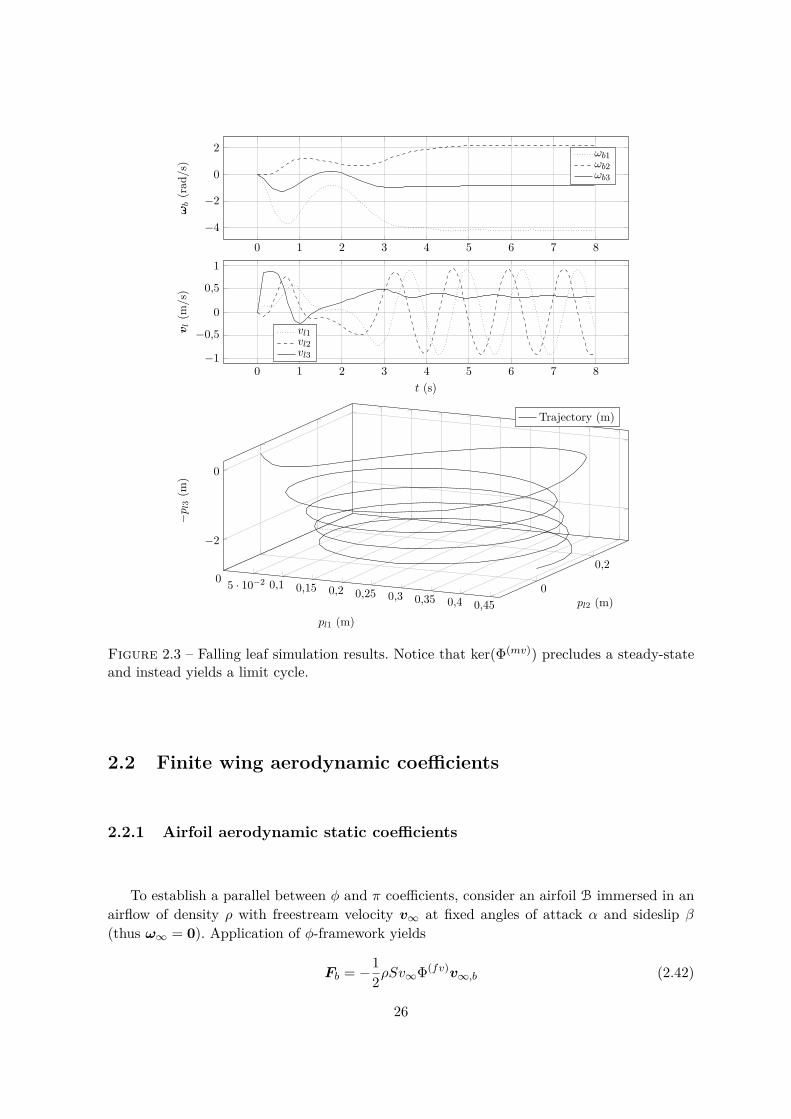
2.3 Falling leaf simulation results. Notice that ker(Φ(mv)) precludes a steady-stateand instead yields a limit cycle. . . . . . . . . . . . . . . . . . . . . . . . . . . 26

2.4 The elliptical drag polar concept allows for rough global qualitative visualiza-tion of aerodynamic forces in arbitrary angles of attack. Firstly, identify bφ,aφ1 and aφ2 and sketch the ellipse accordingly. Secondly, identify the forcedirection by drawing a 2α arc from aφ1 (counterclockwise). The aerodynamicforce Fw is parallel to the line connecting the end of the arc to the origin. Twoexamples are shown : transition and hover. . . . . . . . . . . . . . . . . . . . 29

2.5 The elliptical polar framework applied to thin symmetric airfoils. On the left,a freestream velocity with α incidence is applied. Notice that the associatedpolar has radius R = π. On the right the author suggests a phase-shift as apossibility for aileron modeling. . . . . . . . . . . . . . . . . . . . . . . . . . . 31

2.6 MH45 airfoil with associated thin airfoil approximated aerodynamic center. Inthis example, ∆r < 0 and the center of mass is ahead of the aerodynamiccenter. Additionally, the illustrated choice of body axes will be consistentlyfollowed throughout this thesis. . . . . . . . . . . . . . . . . . . . . . . . . . . 31

3.1 Perspective view, body-axis definition and actuation inputs for a typical tilt-body vehicle representation. . . . . . . . . . . . . . . . . . . . . . . . . . . . . 36

3.2 Propeller wing interaction : slipstream wake illustration and the division bet-ween dry and wet sections. . . . . . . . . . . . . . . . . . . . . . . . . . . . . 36

3.3 In the wet wing region, resulting aerodynamics – namely induced relative airvelocity v∞,i and induced angle of attack αi – are a superposition of freestreamv∞,i and induced propeller wake vi. . . . . . . . . . . . . . . . . . . . . . . . 37

vii

3.4 To the left, SabRe (Soufflerie bas Reynolds) closed-loop wind tunnel facility.To the right, the MAVion wind tunnel model under testing. . . . . . . . . . . 44

3.5 MAVion wind tunnel model instrumentation. . . . . . . . . . . . . . . . . . . 45

3.6 Wind tunnel acquisition system set-up. . . . . . . . . . . . . . . . . . . . . . . 45

3.7 Longitudinal cruise points for a given test vehicle. . . . . . . . . . . . . . . . 46

3.8 Quasi-static equilibrium transition maneuvers and hovering over ground targetunder non-windy (left) and windy (right) conditions. . . . . . . . . . . . . . . 47

3.9 Lateral-directional equilibrium polars. . . . . . . . . . . . . . . . . . . . . . . 48

3.10 Lateral-directional equilibrium polars. . . . . . . . . . . . . . . . . . . . . . . 49

3.11 Lateral-directional equilibrium polars. . . . . . . . . . . . . . . . . . . . . . . 50

3.12 Input assignments of standard RC radio modes. Notice that ψ, Vx, Vz and Vydenote, respectively, desired heading with respect to geographic North, forwardvelocity, vertical velocity and lateral velocity. . . . . . . . . . . . . . . . . . . 50

4.1 The MAVion version employed throughout this thesis. . . . . . . . . . . . . . 53

4.2 MAVion physical dimensions in mm (without winglets). . . . . . . . . . . . . 54

4.3 MAVion avionics integration architecture. . . . . . . . . . . . . . . . . . . . . 56

5.1 To steer x from x(0) towards x0, controller K1 is employed until x reaches R0.Afterwards, controller K0 drives x towards the desired setpoint. . . . . . . . . 60

5.2 Sequence of scheduled controllers K0:N and respective regions-of-attractionR0:N , for N = 3. . . . . . . . . . . . . . . . . . . . . . . . . . . . . . . . . . . 61

5.3 Desired quasi-static trajectory xd(s) and illustrative iterations of the regions-of-attraction based switching linear control algorithm. . . . . . . . . . . . . . 62

5.4 Illustration of the hypothesis : a sequence of controllers Ki where si fail toconverge to 1. . . . . . . . . . . . . . . . . . . . . . . . . . . . . . . . . . . . . 63

5.5 An example of a feasible trajectory starting and ending at the underactuatedregion U. . . . . . . . . . . . . . . . . . . . . . . . . . . . . . . . . . . . . . . 64

5.6 Phase portrait of closed-loop f(x,−Ki∆xi) when ∆xi(ti) ∈ Π+. . . . . . . . 68

5.7 Phase portrait of closed-loop f(x,−Ki∆xi) when ∆xi(ti) ∈ Π−. . . . . . . . 68

5.8 Sequence of RoA-GS controllers Ki with associated Ri fails to cross the originand reach xf . . . . . . . . . . . . . . . . . . . . . . . . . . . . . . . . . . . . . 69

viii

5.9 Numerical stability of the reduced formulation of the linearized quaternionLQR by means of the contour curves of log(log(log(c))). Three log levels are em-ployed due to ill-conditioning and exponentially growing conditioning numberof the reduced model Riccati equation. The two other methods yield constantconditioning over all configuration space and are equal to crel = −0.49688 andcrel = −0.42785 for the transformed reduced and VSI models, respectively. . . 75

5.10 Tracking of an ω-trajectory with transformed reduced quaternion model. . . . 78

5.11 Block diagram of the MATLAB/Simulink simulation setup. . . . . . . . . . . 80

5.12 Simulation reference trajectory in terms of desired forward velocity vf anddesired heading rate ψ. . . . . . . . . . . . . . . . . . . . . . . . . . . . . . . . 81

5.13 Tracking errors in linear velocity ∆vb, angular velocity ∆ωb and attitude ψ forthe defined flight profile without wind disturbances. . . . . . . . . . . . . . . 82

5.14 Actuator u values for the defined flight profile without wind disturbances. . . 83

5.15 Tracking errors in linear velocity ∆vb, angular velocity ∆ωb and attitude ψ forthe defined flight profile under wind disturbances. . . . . . . . . . . . . . . . . 84

5.16 Actuator u∗ values for the defined flight profile under wind disturbances. . . 85

6.1 Reference frames illustration. The inertial (I), body (B) and computed (C)frames are fixed, respectively, to Earth, IMU and estimated orientation by theattitude complementary filter. . . . . . . . . . . . . . . . . . . . . . . . . . . 89

6.2 EMI effect in magnetometers and attitude estimation (without magnetic bias∆b estimation) due to DC motor actuation. . . . . . . . . . . . . . . . . . . . 91

6.3 Input-output schematic view of the quaternion complementary filter. . . . . . 92

6.4 CF-EKF filter overall architecture. . . . . . . . . . . . . . . . . . . . . . . . . 97

6.5 Block diagram of the MATLAB/Simulink simulation setup for the CF stan-dalone experiment. . . . . . . . . . . . . . . . . . . . . . . . . . . . . . . . . . 98

6.6 Block diagram of the MATLAB/Simulink simulation setup for the CF-EKFalgorithm experiment. . . . . . . . . . . . . . . . . . . . . . . . . . . . . . . . 99

6.7 Simulation reference trajectory in terms of desired forward velocity vf anddesired heading rate ψ. . . . . . . . . . . . . . . . . . . . . . . . . . . . . . . . 100

6.8 Navigation errors in velocity δvi and attitude ψ while performing the designa-ted flight profile. . . . . . . . . . . . . . . . . . . . . . . . . . . . . . . . . . . 100

7.1 Block diagram of the MATLAB/Simulink simulation setup for the experiment. 102

ix

7.2 Flight simulation results with a single LQR controller. . . . . . . . . . . . . . 104

7.3 Flight simulation results with a scheduled LQR controller. . . . . . . . . . . . 105

7.4 Flight experiment results with a single LQR controller. . . . . . . . . . . . . . 106

7.5 Flight experiment results with gain-scheduled LQR controllers. . . . . . . . . 107

x

Liste des tableaux

3.1 Flight variables range tested in wind tunnel. . . . . . . . . . . . . . . . . . . . 44

4.1 Flying prototype mass breakdown. . . . . . . . . . . . . . . . . . . . . . . . . 55

6.1 Avionics subset for loosely-coupled GNSS and magnetometer aided strapdowninertial navigation. . . . . . . . . . . . . . . . . . . . . . . . . . . . . . . . . . 90

A.1 Falling leaf simulation parameters . . . . . . . . . . . . . . . . . . . . . . . . . 111

xi

Acronyms

ADC Analog-digital converterAPC Advanced precision compositesAR Aspect ratioCF Complementary filterCFD Computational fluid dynamicsDC Direct currentDCM Direction cosine matrixDOF Degrees of freedomEKF Extended Kalman filterEMI Electromagnetic interferenceESC Electronic speed controlFFS Free fall dynamic systemGNSS Global navigation satellite systemHAV Hybrid aerial vehiclesI2C Inter-integrated circuitIMU Inertial measurement unitINS Inertial navigation systemISAE Institut supérieur de l’aéronautique et de l’espaceJAXA Japan aerospace exploration agencyLLA Latitude, longitude and altitudeLOC Loss of controlLQR Linear quadratic regulatorMAV Micro aerial vehicleMIMO Multiple-input and multiple-outputPPM Pulse position modulationPWM Pulse width modulationQTW Quad-tilt-wingRC Radio controlRPM Revolutions per minuteSDP Semidefinite programmingSO(3) Special orthogonal groupso(3) Special orthogonal group Lie algebra

xiii

SOS Sums-of-squaresTBV Tilt-body vehicleTBVS Tilt-body vehicle systemUART Universal asynchronous receiver/transmitterUAV Unmanned autonomous vehiclesVTOL Vertical take-off and landingWBS Weightless body dynamic systemWGS World geodetic system

xiv

Abstract (English)

Remote building intrusion missions in complex urban environments call for micro airvehicles (MAVs) capable of switching between long-endurance and hover flight modes. Tra-ditionally, long-endurance missions are performed by fixed-wing architectures which advan-tage from lift generation due to aerodynamic surfaces. This yields high-speed stable flighteven under adverse wind conditions. On the other hand, hovering platforms (e.g., multi-rotorplatforms, helicopters) cannot benefit from air to vehicle relative movement and calls forenergetically expensive propulsion methods that precludes long-distance missions but allowsfor sustained low-speed unstable indoor flight. This thesis is built around a hybrid architec-ture based on the tilt-body tail-sitting concept, called MAVion, that is capable of balancingaerodynamic and propulsion design parameters to deliver a solution to the remote buildingintrusion problem.

Since their debut in the 50s, vertical take-off and landing (VTOL) aircraft would only beflown by the most experienced pilots. Recent advances on low-cost inertial sensors, embeddedcomputing and control technology – on the other hand – support stability augmentation sys-tems (SAS) in mitigating unstable dynamic modes and allowing for inexperienced (or evenautonomous) flight. Nearly all autopilot design techniques, however, rely on accurate mathe-matical descriptions of novel and thus unfamiliar architectures (e.g., number and positioningof propellers, number and positioning of fixed/variable aerodynamic surfaces). While a largeand growing body of literature has investigated underlying modeling, control and planningissues to specific hybrid vehicles, an unified approach to addressing arbitrary architecturesis practically non-existent. The present thesis establishes an unified framework, namely theφ-theory, for assessing hybrid vehicles handling qualities and, moreover, designing appropriatestabilizing control laws.

This study sets out to establish a tractable model for tail-sitting vehicles in view of controldesign and qualitative dynamics analysis. The proposed φ-theory not only yields a numericallyadvantageous model but also extends our comprehension of tail-sitting vehicles. In sharpcontrast with existent literature, the proposed model is globally non-singular, polynomial-like and bypasses the use of aerodynamic angles of attack and sideslip (both free-stream andpropwash-induced !). Nevertheless, even if mathematically elegant, a mathematical model haspractical use only if consistent with reality. This thesis shows this is the case by meansof wind tunnel data and flight experiments. I strongly believe φ-theory provides a fittingbalance between model complexity and controller design simplicity. I prove this point bytuning MAVion’s controller in simulation and test-flying it in reality – with a novel aidedinertial navigation technique – without resorting to further exhausting experimental tuningcampaigns.

1

Abstract (French)

Les missions confiées aux drones sont de plus en plus nombreuses. Par exemple le survol oul’intrusion dans un bâtiment à distance dans des environnements urbains complexes exigentdes micro-véhicules aériens (MAV) capables de basculer entre un mode de vol économique(endurance) et un mode stationnaire (survol). Traditionnellement, les missions d’enduranceprolongée sont réalisées par des architectures à voilure fixe de type avion qui bénéficient dede la portance grâce aux surfaces aérodynamiques. Cela permet un vol à grande vitesse quireste stable même dans des conditions de vent difficiles. D’autre part, les plates-formes àvoilure tournante (par exemple, les plates-formes multi-rotor, les hélicoptères) ne peuventpas bénéficier d’un mouvement relatif de l’air vers le véhicule et nécessitent l’utilisation deméthodes de propulsion énergiquement coûteuses qui limitent fortement l’autonomie maispermettent un vol stationnaire. Cette thèse s’articule autour d’une architecture hybride trèssimple mécaniquement basée sur le concept tilt-body, appelée MAVion, capable d’équilibrerles paramètres de conception aérodynamique et de propulsion pour résoudre le problème del’intrusion à distance.

A leurs débuts dans les années 50, les véhicules de décollage et d’atterrissage verticaux(VTOL) n’étaient pilotés que par les pilotes les plus expérimentés. Les avancées récentes surles capteurs inertiels à faible coût, les systèmes embarqués intégrés, d’autre part, renforcent lessystèmes d’augmentation de la stabilité (SAS) pour atténuer les modes dynamiques instableset permettre un vol par un utilisateur faiblement expérimenté puis de façon totalement auto-nome. Cependant, presque toutes les techniques de conception du pilote automatique reposentsur des descriptions mathématiques précises d’architectures nouvelles et donc inconnues (parexemple, nombre et positionnement des hélices, nombre et positionnement des surfaces aé-rodynamiques fixes / variables). Alors qu’un nombre croissant d’études dans la littératures’intéresse aux problèmes sous-jacents de la modélisation, du contrôle et de la planificationdes véhicules hybrides spécifiques, une approche unifiée pour aborder les architectures ar-bitraires est pratiquement inexistante. La présente thèse établit un cadre unifié, à savoirla φ-théorie, pour évaluer les qualités de manipulation des véhicules hybrides et, en outre,concevoir des lois de contrôle stabilisatrices appropriées.

Cette étude a consisté à établir un modèle traçable pour les véhicules tail-sitters en vue dela conception du contrôle et de l’analyse de la dynamique qualitative. La φ-théorie proposéene donne pas seulement un modèle avantageusement numérique, mais élargit également notrecompréhension des véhicules tail-sitters. En contraste étroit avec la littérature existante, lemodèle proposé est globalement non singulier, de type polynomial et contourne l’utilisationd’angles aérodynamiques d’attaque et de glissement latéral (free-stream et propwash induits).Même si mathématiquement élégant, un modèle mathématique ne présente un intérêt que s’ilest conforme à la réalité. Cette thèse montre que c’est le cas au moyen de données issues d’unecampagne de soufflerie ainsi que grâce à des essais en vol. Je crois fermement que la φ-théorieoffre un équilibre approprié entre la complexité du modèle et la simplicité de la conceptiondu contrôleur. Ceci est démontré dans la thèse en appliquant cette théorie au MAVion dans

3

la simulation et le testant en réalité - avec une nouvelle technique de navigation inertielleassistée - sans recourir à d’autres campagnes expérimentales afin de régler les gains de façonexpérimentales, ce qui est couramment le cas dans le domaine des micro et mini drones.

4

Chapitre 1

Introduction

Sommaire1.1 A glimpse at the hybrid aerial vehicles (HAV) landscape . . . . . . . 51.2 HAV modeling and control design state of the art . . . . . . . . . . . . 71.3 Thesis motivation . . . . . . . . . . . . . . . . . . . . . . . . . . . . . . . 101.4 Thesis roadmap . . . . . . . . . . . . . . . . . . . . . . . . . . . . . . . . 10

1.4.1 Problem statement . . . . . . . . . . . . . . . . . . . . . . . . . . . . . . . 101.4.2 Thesis contributions . . . . . . . . . . . . . . . . . . . . . . . . . . . . . . 111.4.3 Thesis structure . . . . . . . . . . . . . . . . . . . . . . . . . . . . . . . . 11

1.5 Notation . . . . . . . . . . . . . . . . . . . . . . . . . . . . . . . . . . . . . 11

1.1 A glimpse at the hybrid aerial vehicles (HAV) landscape

We hold this truth to be self-evident : unmanned aerial vehicles (UAVs) are an enablingtechnology. Numerous different architectures are available for fulfilling a myriad of distinct –and often conflicting – purposes. Until very recently, most commercial UAVs were categorizedas either fixed-wing or rotary-wing (multi-copters). While fixed-wing designs are known fortheir substantial endurance, rotary-wings are notable for their hovering capabilities. A thirdcategory that emerged aiming at bridging those incompatible features has recently caughtthe attention of scientists and engineers, namely : the hybrid aerial vehicles (HAVs). Eventhough HAVs are long-established (take, for instance, the 1963 early works regarding tilt-wing vehicles [Fay63], lifting fans [Asm63] and tilt-propeller vehicles [Bor63]), piloting of earlydesigns was demanding [GE63] and unsafe [Sch63] thus precluding wide commercial viability– until now. Recent advances in low-cost inertial sensors and embedded computing boostedthe development of stabilizing control systems that allow for stable and safe HAV piloting.Indeed, micro HAVs are starting to find their way into consumer and business markets – e.g.,the off-the-shelf Parrot Swing and the Wingtra WingtraOne, respectively (see Fig. 1.1).

From an academic perspective, the Japan Aerospace Exploration Agency (JAXA) has beeninvestigating the practical viability of vertical take-off and landing (VTOL) aircraft as futuremeans to civil transportation. For instance, [Tot+16] proposes a HAV of type quad-tilt-wing(QTW). The QTW vehicle is a VTOL aircraft equipped with four propeller units installed onfour separate (tandem configuration) wings. To transition between hover and cruise nominal

5

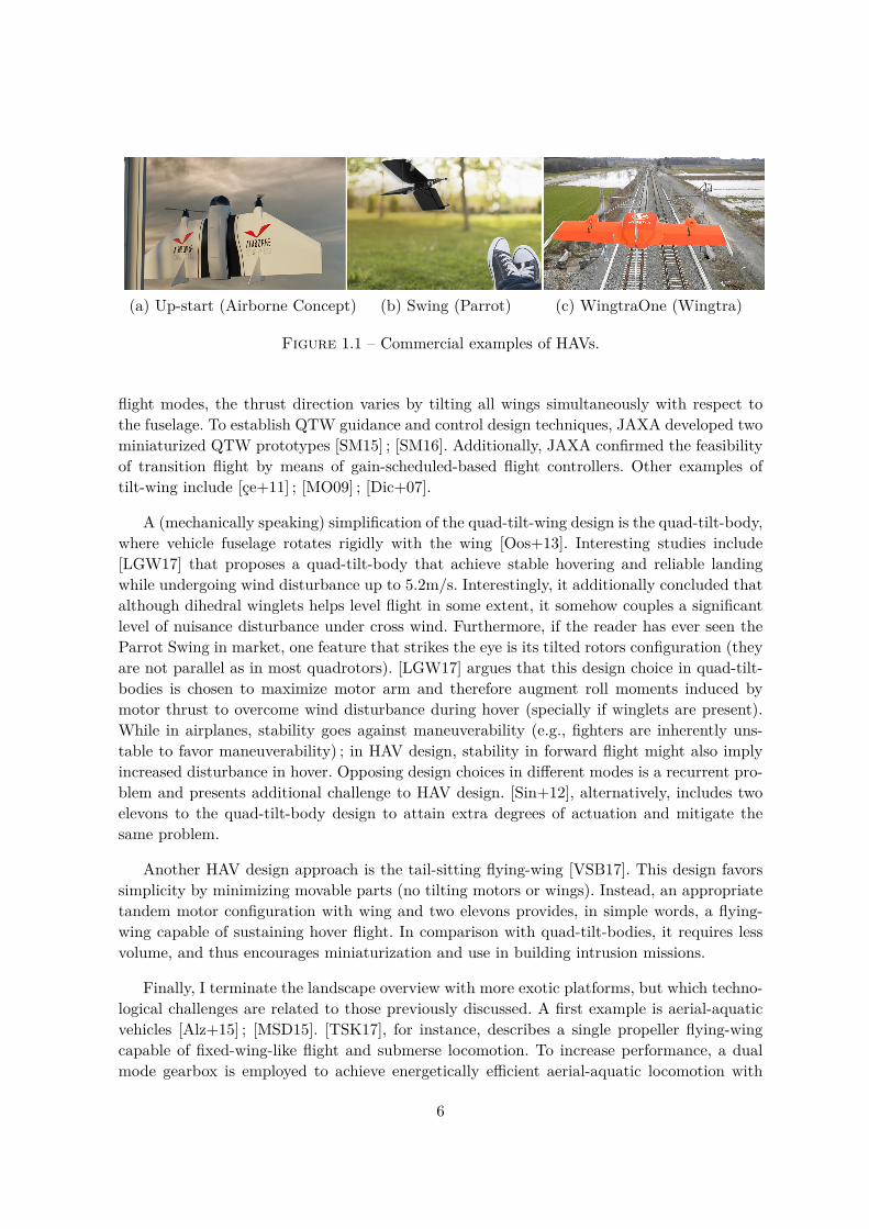
(a) Up-start (Airborne Concept) (b) Swing (Parrot) (c) WingtraOne (Wingtra)

Figure 1.1 – Commercial examples of HAVs.

flight modes, the thrust direction varies by tilting all wings simultaneously with respect tothe fuselage. To establish QTW guidance and control design techniques, JAXA developed twominiaturized QTW prototypes [SM15] ; [SM16]. Additionally, JAXA confirmed the feasibilityof transition flight by means of gain-scheduled-based flight controllers. Other examples oftilt-wing include [çe+11] ; [MO09] ; [Dic+07].

A (mechanically speaking) simplification of the quad-tilt-wing design is the quad-tilt-body,where vehicle fuselage rotates rigidly with the wing [Oos+13]. Interesting studies include[LGW17] that proposes a quad-tilt-body that achieve stable hovering and reliable landingwhile undergoing wind disturbance up to 5.2m/s. Interestingly, it additionally concluded thatalthough dihedral winglets helps level flight in some extent, it somehow couples a significantlevel of nuisance disturbance under cross wind. Furthermore, if the reader has ever seen theParrot Swing in market, one feature that strikes the eye is its tilted rotors configuration (theyare not parallel as in most quadrotors). [LGW17] argues that this design choice in quad-tilt-bodies is chosen to maximize motor arm and therefore augment roll moments induced bymotor thrust to overcome wind disturbance during hover (specially if winglets are present).While in airplanes, stability goes against maneuverability (e.g., fighters are inherently uns-table to favor maneuverability) ; in HAV design, stability in forward flight might also implyincreased disturbance in hover. Opposing design choices in different modes is a recurrent pro-blem and presents additional challenge to HAV design. [Sin+12], alternatively, includes twoelevons to the quad-tilt-body design to attain extra degrees of actuation and mitigate thesame problem.

Another HAV design approach is the tail-sitting flying-wing [VSB17]. This design favorssimplicity by minimizing movable parts (no tilting motors or wings). Instead, an appropriatetandem motor configuration with wing and two elevons provides, in simple words, a flying-wing capable of sustaining hover flight. In comparison with quad-tilt-bodies, it requires lessvolume, and thus encourages miniaturization and use in building intrusion missions.

Finally, I terminate the landscape overview with more exotic platforms, but which techno-logical challenges are related to those previously discussed. A first example is aerial-aquaticvehicles [Alz+15] ; [MSD15]. [TSK17], for instance, describes a single propeller flying-wingcapable of fixed-wing-like flight and submerse locomotion. To increase performance, a dualmode gearbox is employed to achieve energetically efficient aerial-aquatic locomotion with

6

a single propeller. Similarly, [PTD17] provides a flying-wing capable of vertical takeoff andlanding on water. A summary of aerial-aquatic vehicles is described in [Yan+15].

1.2 HAV modeling and control design state of the art

To the extent of the author’s knowledge, the Pixhawk autopilot is currently the onlyopensource system to implement HAV control laws. In it, hover and cruise mode controllers areseparately implemented as, respectively, multi-copter and fixed-wing traditional controllers.During a transition, those are interchanged and an ad hoc blending algorithm attempts tosmooth the resulting switching transient. It is worth noticing, however, the following comment(which my experience firmly supports) posted 1 in their HAV website : "The current code basepaves the road for VTOL applications but it is still in its early phase. At this moment you willprobably need a good understanding of the PX4 code base and some flying skills to operate thecaipirinha VTOL successfully. We are putting a lot of effort into developing the VTOL codebase further." Recent examples of such transition flight control strategy are found in [KZW17].[KZW17] is particular in its way to switch not only control laws but also Euler angles definitionin order to avoid attitude singularities. Most other work, however, use quaternion as global(and numerically stable) attitude parametrization.

This thesis pursues an approach similar to [HMM17] ; [RD17] ; [LGW17], for which transi-tion flight is not considered as a temporary (and in some sense undesirable) transient betweenflight modes, but as a functional flight mode in itself. In this point of view, the pilot is able tostabilize the vehicle at a continuum set of forward velocities from zero (hovering) to nominalcruise speed. It is the controller responsibility to abstract the velocity commands to adequateattitude and actuator references – even if that means stabilizing at post-stall angles of attack.This upholds the usefulness of adequate post-stall modeling.

From the point of view of HAV modeling for control design, [HMM17], for instance, em-ploys lookup tables – obtained by means of typically lengthy static wind tunnel campaigns –to design gain-scheduled controllers without resorting to an analytical mathematical model.A similar approach is employed in [SM15] ; [SM16]. On the other hand, [LGW17] fits windtunnel data to a given aerodynamic coefficient formula in function of angle-of-attack α toobtain analytical models. Additionally, dynamic coefficients call for even more complex windtunnel campaigns or complex flight instrumentation [Sme+14]. If low-cost instrumentation isapplied and data synchronization is prohibitively expensive, recent work [Mor17] proposes amethod for dynamic coefficient identification from flight data with unknown clock (timing)skews. Furthermore, it goes without saying that not only parametric identification takes aplace in modeling. [Hal+17] discusses (and provides methods for measuring) uncertaintiesdue to the assumed aerodynamics coefficients algebraic model form. An interesting contri-bution – closely related to the driving philosophy I follow herein – is found in [Puc13]. Init, the aerodynamic coefficient algebraic structure is constrained to a carefully chosen familyof functions to promote global nonlinear control design. In this thesis, however, I restrain

1. Friday, August 25, 2017 2 :40 PM (GMT+2) @ pixhawk.org/platforms/vtol/tbs_caipirinha_vtol.

7

aerodynamic coefficient structure to promote algorithmic control design.

This thesis employs a steady-state approach to modeling aerodynamic coefficients, that is,I neglect dynamic vortex-shedding processes [US17], in which a rapid increase in the angle-of-attack causes the formation of a leading-edge vortex that produces an unsteady increasein lift that decays as the vortex is convected downstream. In this scenario, aerodynamiccoefficients are dependent on the past history of angles-of-attack and sideslip. In previouswork [GK94] ; [FL96] ; [Fis95] ; [SJ96] ; [Sin+13] ; [Rei+11] ; [PLG13] ; [Gre04], modeling isachieved by means of an augmented system state that includes a flow separation parameter. Bypursuing at first the steady-state approach, I am able to identify which HAV phenomena arequalitative describable by this simplified approach, and which phenomena require augmentedorder systems.

Another approach to dealing with aerodynamic coefficients uncertainty is to employ adap-tive control laws. In [RD17], for instance, flight experiments were conducted by employingmachine learning techniques to estimate tilt-body aerodynamic parameters of a first-principlesmodel and adapting the controller accordingly.

Since winged HAVs often operates in post-stall regions, a lot of knowledge is promptlyavailable in aircraft loss of control (LOC) literature. For instance, [Fri+17] summarizes thestatus of ongoing NASA research to advance augmented flight simulation models for civil air-craft LOC due to wing stall for pilot training purposes. This paper is particularly interestingsince it addresses the ever-present challenge of creating nonlinear reduced-order models fromhigh-fidelity computational data and flight experiments, which is the core philosophical basisof the present thesis. Also, I would like to cite here [Fri+17] and their remarks on computa-tional fluid dynamics (CFD) current capabilities in view of different flight regimes : "Aftereight years of focused collaboration among a diverse international body of computational andexperimental aerodynamicists and flight simulation experts, the resounding conclusion wasthat, although current CFD methodology could readily predict the S&C [stability and control]behavior of aircraft flying in linear regions of a flight envelop, it is still extremely difficult toadequately capture the static and dynamic S&C characteristics associated with highly nonlinearflows." Nevertheless, there are recent efforts [Car+17] towards providing a computational fluiddynamics technique to predict aerodynamic dynamic damping of HAVs. Finally, recent stu-dies in LOC in commercial airliners are based either in the NASA Generic transport (GTM)[Gil+13] or the European SUPRA models [Abr+12], and it has revealed a deeper unders-tanding of the spiral dives and steep spins exhibited by these models by applying standardautopilot controllers to outside the flight envelope conditions [Gil+15].

Most fixed-wing controllers found in the literature decouple lateral and longitudinal dy-namics so that separate modeling and control design take place independently. However,[HDB16] analyses coupling effects between lateral and longitudinal dynamics of a tail-sittingflying-wing and concludes that unstable spiral dynamics are incorrectly rendered stable bydecoupling assumptions. This suggests that coupled dynamics is fundamental for HAVs andmultiple-input multiple-output (MIMO) control design should be favored. [LGW17], for ins-tance, employs a cascade control composed of MIMO outer loop nonlinear exponential stableangle [BM95] and MIMO inner PID angular velocity loops.

8

With the advance of fast and reliable embedded computing systems, algorithmic controltheory [TM17] has been put in evidence in recent years. This theory departs from the usualfixed-algebraic structure controller to a state-error-to-actuator mapping implicitly computedby an (often convex optimization solver) algorithm. Recent examples related to HAVs include[FMH02] ; [MCT14]. The present thesis promotes this line of thought by providing – in addi-tion to other features – optimization-solver-friendly dynamic models of HAVs. In addition tocontrol design, optimization techniques allows for efficient aerodynamics model identification,such as in [VC+16], where a technique is proposed for post-flight wind estimation in the ab-sence of air-data sensors. Once the wind speed is estimated, flight data is corrected and usedto perform aerodynamic coefficient estimation. I note that, if efficient optimization routinesare available, this same technique can be applied in real-time for in-flight wind perturbationcompensation. [DVS17], on the other hand, employs Kalman filtering for computationally-cheap wind estimation without pitot tube for flying-wing tail-sitters with 5% wind speedand 7o wind direction accuracy. While pitot tube is instrumental for fixed-wings [Cho+11],the wide envelope of angle-of-attacks found on tilt-bodies preclude their use, and techniquessuch as the one just mentioned are of utmost necessity. To the best of the author’s know-ledge, the latter is the only work on wind estimation on-board tilt-bodies. Previous work onmodel-based wind estimation for hovering multi-copters are [SCW16] ; [Bur+15] ; [Neu+12] ;[Abe+14] ; [WW09] ; [Sch+14].

Additionally, most current HAV model differential equations are immensely general withno special structure that could be exploited in specialized optimization solvers. [VSB17], forinstance, employs a multi-purpose optimization tool to search for feasible tilt-body cruise-to-hover trajectories while optimizing a certain cost function. The present thesis, however, aimsat modeling HAVs from physics principles and algebraic restrictions to obtain singularity-free systems which possess special structure in view of pursuing efficient (and thus real-time)optimization.

While oblique-flow propeller modeling is fundamental for flight performance analysis, itsrelevance to feedback control design is disputable. Furthermore, incidence propeller modelingis intricate and often requires wind tunnel campaigns. For instance, [The+17] shows thatwhile the traditional combo of blade element momentum theory, vortex lattice method, andmomentum theory for oblique flow is a commonplace tool for helicopter design, it fails toproperly reflect wind tunnel data in high angles of incidence.

Finally, I did not feel the need to consider flexible structural dynamic modes while deve-loping the experimental part for ISAE’s particular drone, and I refer the reader to [Sch16]for a recent flexible flying-wing case study. I remark that while I believe flexibility effects donot represent a problem in nominal HAV flight control design, it does defines the nominalflight itself. [KSK17] ; [Kun05] acknowledge that cruise speed and range are limited directly orindirectly by proprotor/pylon/wing structural stability, known as whirl flutter, an importantdesign consideration for tilt-rotor aircraft.

9

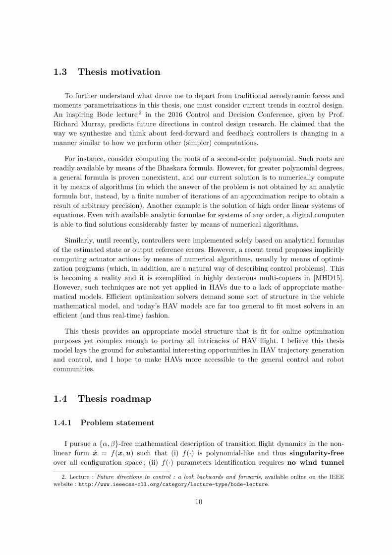
1.3 Thesis motivation

To further understand what drove me to depart from traditional aerodynamic forces andmoments parametrizations in this thesis, one must consider current trends in control design.An inspiring Bode lecture 2 in the 2016 Control and Decision Conference, given by Prof.Richard Murray, predicts future directions in control design research. He claimed that theway we synthesize and think about feed-forward and feedback controllers is changing in amanner similar to how we perform other (simpler) computations.

For instance, consider computing the roots of a second-order polynomial. Such roots arereadily available by means of the Bhaskara formula. However, for greater polynomial degrees,a general formula is proven nonexistent, and our current solution is to numerically computeit by means of algorithms (in which the answer of the problem is not obtained by an analyticformula but, instead, by a finite number of iterations of an approximation recipe to obtain aresult of arbitrary precision). Another example is the solution of high order linear systems ofequations. Even with available analytic formulae for systems of any order, a digital computeris able to find solutions considerably faster by means of numerical algorithms.

Similarly, until recently, controllers were implemented solely based on analytical formulasof the estimated state or output reference errors. However, a recent trend proposes implicitlycomputing actuator actions by means of numerical algorithms, usually by means of optimi-zation programs (which, in addition, are a natural way of describing control problems). Thisis becoming a reality and it is exemplified in highly dexterous multi-copters in [MHD15].However, such techniques are not yet applied in HAVs due to a lack of appropriate mathe-matical models. Efficient optimization solvers demand some sort of structure in the vehiclemathematical model, and today’s HAV models are far too general to fit most solvers in anefficient (and thus real-time) fashion.

This thesis provides an appropriate model structure that is fit for online optimizationpurposes yet complex enough to portray all intricacies of HAV flight. I believe this thesismodel lays the ground for substantial interesting opportunities in HAV trajectory generationand control, and I hope to make HAVs more accessible to the general control and robotcommunities.

1.4 Thesis roadmap

1.4.1 Problem statement

I pursue a {α, β}-free mathematical description of transition flight dynamics in the non-linear form x = f(x,u) such that (i) f(·) is polynomial-like and thus singularity-freeover all configuration space ; (ii) f(·) parameters identification requires no wind tunnel

2. Lecture : Future directions in control : a look backwards and forwards, available online on the IEEEwebsite : http://www.ieeecss-oll.org/category/lecture-type/bode-lecture.

10

nor computer fluid dynamics computations for designing a preliminary stable autopilot ;(iii) f(·) simple structure encourages nonlinear feedback design and efficient feed-forwardplanning/optimization ; (iv) provides insight into the vehicle qualitative dynamics and (v)can be validated by means of wind tunnel campaigns and flight experiments.

1.4.2 Thesis contributions

Theoretical contributions : The φ-theory framework is proposed for hybrid vehiclesmodeling. Its mathematical properties and features are thoroughly studied. The present thesisshows that φ-theory-based models concur with (i)-(iv) in Sec. 1.4.1.

Experimental contributions : This thesis contrasts wind tunnel data to theoreticalfindings to assess φ-theory suitability in real world. Experimental flights call for state estima-tors that rely on low-cost navigation sensors. For that, the present thesis studies a novel stateestimator architecture that lays the foundation for aided inertial navigation that employscomplementary filtering for attitude estimation by means of a magnetometer as an externalaid, and an EKF for additional sensors integration. Finally, a Paparazzi-based prototype isintegrated and flight-tested to illustrate the effectiveness of my approach.

Additionally, this thesis motivated the following publications : [LDMde] ; [LDM17] ; [Lus+17] ;[Lus+16] ; [Alh+16] ; [LDM15] ; [LDM14] ; [MLD14].

1.4.3 Thesis structure

This document is divided in two parts. Part I proposes φ-theory as an optimization-friendlyparametrization of aerodynamic forces and moments. Chap. 2 introduces the main conceptsand results that underlie φ-theory employment in modeling aerodynamic forces and momentson an airfoil. Interesting insights are additionally revealed on wing-propeller interaction mo-deling. Chap. 3 employs the φ-theory basic notions to tail-sitting flying-wing modeling, anddiscuss qualitative results of this type of HAV flight.

Part II describes the experimental flight campaigns conducted to validate the φ-theoryapproach in reality. Chap. 4 overviews the particular platform employed in my studies. Chap.5 discusses several issues involved in control design of HAVs, and ultimately provides a controlarchitecture for velocity-controlled piloting. Chap. 6 provides some studies conducted in stateestimation, and ultimately describes the drone navigation routine (and the choices involvedfor using it). Finally, Chap. 7 illustrates my experimental findings.

1.5 Notation

In this thesis, kinematic quantities of interest in multiple moving reference frames are rigo-rously studied and, consequently, a consistent and precise notation is called for. Accordingly,

11

this section outlines notation conventions including related variables of interest.

The notation axc is employed, where the symbol x denotes desired vector quantity (e.g., pfor position, v for velocity, a for acceleration, ω for angular velocity) of point/frame (dependingon the context) C with respect to frame A. For instance, iωb denotes angular velocity of aframe B with respect to a frame I. Additionally, the decomposition of a vector x ∈ Rn intoits components in a frame R is denoted by means of the right subscript position, e.g.

xr =(xr1 xr2 · · · xrn

)T(1.1)

and its magnitude by discarding the bold font, e.g.,

x =√xTr xr (1.2)

We remark that all reference frames {F} of interest in this thesis – unless otherwise stated– are right-handed, orthonormal and, hence, isomorphic to the well-known SO(3) group,where

SO(3) = {D ∈ R3×3 : DDT = I, detD = +1} (1.3)

In the following, we make extensive use of the vector product operation. Its matrix repre-sentation [vb×] ∈ so(3) (in some basis B) is denoted by

vb× = [vb×] =

0 −vb3 vb2vb3 0 −vb1−vb2 vb1 0

(1.4)

We shall not elect a best attitude parametrization but, instead, use them all interchan-geably during this thesis. Quaternion algebra structure definition varies to a small extent inliterature. Herein, a quaternion algebra (Q,×) is defined as [SL03]

Q = {q ∈ R4 : 〈q, q〉 = 1} (1.5)

and it is equipped with quaternion product operation × : Q×Q→ Q defined as

p× q =(

p0q0 − p · qp0q + q0p+ p× q

)(1.6)

where, for instance,

q =(q0q

)with q0 ∈ R, q ∈ R3 (1.7)

The quaternion and direction cosine matrix (DCM) from frame A to B, respectively, qab

12

and Dab , are denoted such that their respective rotation formulae [SL03] are written as(

0xb

)= (qab )′ ×

(0xa

)× qab (1.8)

andxb = Da

bxa (1.9)

where (qab )′ denotes the quaternion conjugate of qab .

13

Part I

An introduction to φ-theory

15

Chapitre 2

The φ-theory approach to wingaerodynamics modeling

Sommaire2.1 Aerodynamic forces and moments . . . . . . . . . . . . . . . . . . . . . 17

2.1.1 The classic approach . . . . . . . . . . . . . . . . . . . . . . . . . . . . . . 172.1.2 The φ-theory parametrization . . . . . . . . . . . . . . . . . . . . . . . . . 192.1.3 Application : The falling leaf dance . . . . . . . . . . . . . . . . . . . . . . 25

2.2 Finite wing aerodynamic coefficients . . . . . . . . . . . . . . . . . . . . 262.2.1 Airfoil aerodynamic static coefficients . . . . . . . . . . . . . . . . . . . . 262.2.2 Airfoil aerodynamic derivatives . . . . . . . . . . . . . . . . . . . . . . . . 282.2.3 Application : Thin airfoils . . . . . . . . . . . . . . . . . . . . . . . . . . . 30

2.3 Wing-propeller interaction . . . . . . . . . . . . . . . . . . . . . . . . . . 322.3.1 π-theory wing-propeller interaction [McC98] . . . . . . . . . . . . . . . . . 332.3.2 φ-theory wing-propeller interaction . . . . . . . . . . . . . . . . . . . . . . 33

2.4 Final remarks . . . . . . . . . . . . . . . . . . . . . . . . . . . . . . . . . . 34

2.1 Aerodynamic forces and moments

2.1.1 The classic approach

The ubiquitous Buckingham-π-theorem-based approach [And10] to modeling steady ae-rodynamic forces F ′b ∈ R3 and momentsM ′

b ∈ R3 on a finite wing B immersed in an uniformairflow with freestream velocity v∞ ∈ R3 is traditionally given by

F ′b = 12ρSv

2∞Cb(α, β,M,Re) (2.1)

andM ′

b = 12ρSv

2∞BKb(α, β,M,Re) (2.2)

where

B =

b 0 00 c 00 0 b

(2.3)

17

and b, c, ρ, S ∈ R∗+, Cb, Kb : R4 → R3 denote, respectively, reference wingspan, referencechord, freestream air density, reference finite wing surface, aerodynamic force and momentthree-dimensional coefficients described in body frame B. The latter are function of the di-mensionless quantities α, β, M and Re, namely, angle of attack, sideslip angle, Mach andReynolds numbers. Hereafter v∞ flow is assumed incompressible and inviscid and, therefore,Cb andKb are solely function of α and β during all flight conditions of interest. As previouslydiscussed, Cb(α, β) and Kb(α, β) are often (e.g., [CT08], [Fra+07], [SH09]) modeled as finitetruncated sums of Fourier or Maclaurin series to fit wind tunnel and flight data.

b1b3

Figure 2.1 – The illustrated choice of body axes will be consistently followed throughoutthis thesis for airfoils and wings. Notice that b2 is such that b3 = b1 × b2.

By contrast, φ-theory proposes a novel {α, β}-free parametrization of aerodynamics forcesand moments. To understand the motivation behind this approach, recall that (see Fig. 2.1for body B axes definition)

α = tan−1(v∞,b3v∞,b1

)(2.4)

andβ = sin−1

(v∞,b2v∞

)(2.5)

Tail-sitting and highly manoeuverable flight, however, encounter near-zero freestream veloci-ties (predominantly in wing sections not covered by propeller sliptream) that call for near-zeroalgebraic divisions in (2.4) and preclude numerical stability of digital simulations. Althoughif-else statements with appropriate ad hoc thresholds would solve the issue, notice, however,that

∂α

∂v∞,b1= − v∞,b3

v2∞,b1 + v2

∞,b3(2.6)

and, therefore, ∇α(v∞,b) is not continuous at v∞,b = 0 due to (2.6) and yields a nondiffe-rentiable mapping regardless of the value one defines for α at the singularities of (2.4). Thisproperty hinders linearization-based techniques employment for control and analysis duringhover flight (in which α and β behavior is immensely sensible across dry wing sections).

Additionally, the present thesis attempts to fit local experimental data while simulta-neously striving for satisfactory qualitative global behavior. For instance, notice that a tail-sitter in hover descent encounters an extrinsic α = π in view of traditional airfoil aerodynamicsand calls for coherent aerodynamic coefficient extrapolation capabilities.

Finally, recent efforts [PL03] in semidefinite programming (SDP) and sums-of-squares(SOS) optimization allow for efficient trajectory optimization and control in dynamic modelsgoverned by polynomial differential equations. Traditional aerodynamic coefficients formula-tion carries trigonometric functions that preclude SDP employment and calls for computer

18

expensive path planning routines. Alternatively, φ-theory proposes an SDP-friendly formula-tion.

2.1.2 The φ-theory parametrization

φ-theory is built upon the following {α, β}-free parametrization of aerodynamic forces andmoments :

τ = −12ρSηCΦ(η)Cη (2.7)

where τ , η ∈ R6, η ∈ R+, are, respectively, the aerodynamic wrench (with respect to thecenter of mass), wing twist, and aerodynamic φ-norm given by

τb =(FbMb

)(2.8)

ηb =(v∞,bω∞,b

)(2.9)

andη =

√v2∞ + φc2ω2

∞, φ > 0 (2.10)

where φ ∈ R∗+ is a dimensionless tunable parameter. Furthermore, ω∞,b ∈ R3 denotes halfthe freestream vorticity ξ∞ such that 1

ω∞ = 12ξ∞ = 1

2∇× v∞ (2.11)

In absence of wind, one can easily prove that ω∞ is equal to the vehicle angular velocity.Additionally, the wing screw reference matrix C ∈ R6×6 is an extension of the wing referencematrix concept and it is defined as

C =[I3×3 03×303×3 B

](2.12)

Finally, Φ : R6 → R6×6 is the aerodynamic φ-coefficient. The symbol φ is introducedin the nomenclature to facilitate parallels between the novel parametrization and the tra-ditional Buckingham-Π-based coefficients/derivatives. Additionally, for the sake of brevity,Buckingham-Π-based formulae and coefficients (e.g., CL, CD) are referenced as π-theoryand π-coefficients in the following, while the present model is referenced as φ-theory andφ-coefficients.

1. ω∞ is defined by means of vorticity for the sake of clarity. Nevertheless, although fluid, freestream flowconstitutes a rigid motion and one can think of ω∞ as freestream angular velocity.

19

Unless otherwise stated, Φ(·) is hereafter considered a constant function written as

Φ =[

Φ(fv) Φ(fω)

Φ(mv) Φ(mω)

](2.13)

where Φ(fv), Φ(fω), Φ(mv), Φ(mω) ∈ R3×3. It will be presently shown that such assumptiongreatly simplifies the model and yet still captures dominant features – e.g., post-stall effects,aerodynamic derivatives, global dissipation of energy – over the entire flight envelope (i.e.,hover, cruise and transition flight modes).

Remark 2.1To avoid parameter clutter, 1

2ρSCΦC will occasionally be simply denoted as Φ by abuse ofnotation. The meaning of Φ in any following occurrence should be clear from the context(specially by units inspection). This consideration simplifies (2.7) to read

τ = −ηΦη (2.14)

Some theoretical results follow to support φ-theory employment in wide envelope appli-cations. Then, a falling leaf example illustrates the theory before addressing this thesis mainmotivation, namely, the tilt-body problem.

Remark 2.2 (Structural consistency under transport of forces and moments)Let ΦA be a given aerodynamic φ-coefficient with respect to a point A. Transportation to apoint B yields

τB = τA +[

0 0[rA/Bb ×] 0

]τA =

[I 0

[rA/Bb ×] I

]︸ ︷︷ ︸

R1

τA (2.15)

where rA/B denotes position of point A with respect to point B. Similarly,

ηB = ηA +[0 [rA/Bb ×]0 0

]ηA = R2η

A (2.16)

thus

τB = R1τA = −R1

12ρSη

ACΦACηA = −1

2ρSηAC C−1R1CΦACR

−12 C−1︸ ︷︷ ︸

ΦB

CηB (2.17)

whereΦB = C−1R1CΦACR

−12 C−1 (2.18)

Therefore, φ-structure is preserved under transport of forces and moments if and only ifηA = ηB. That is the case for static wind tunnel measurements (i.e., ω∞ = 0). However,care must be exercised when analyzing and transporting dynamic wind tunnel measurements(e.g., aerodynamic derivatives Clp , Cmq , Cnr). Therefore, for structural consistency, one canimpose φ-norm computation at a fixed point in the body (normally the center of mass), while

20

the screws τ and η are transportable according to (2.18).

Definition 2.1 (Weightless body system)Let B be a rigid-body with inertia (m,J) under influence of aerodynamic forces and momentsin a negligible gravity field with no wind. The weightless body dynamic system (WBS) isdefined as the associated dynamical system given by

vb = 1mFb − [ωb×]vb

ωb = J−1Mb − J−1[ωb×]Jωbτb = −ηΦηb

(2.19)

Definition 2.2 (Free fall system)Let B be a rigid body with inertia (m,J) by influence of aerodynamic forces and moments ina constant (w.r.t inertial frame L) gravity field gl 6= 0 with no wind. The free fall dynamicsystem (FFS) is defined as the the associated dynamical system given by

vb = 1mFb +Dl

bgl − [ωb×]vbωb = J−1Mb − J−1[ωb×]JωbDlb = −[ωb×]Dl

b

τb = −ηΦηb

(2.20)

Definition 2.3 (Terminal states and terminal velocities)The set of terminal states T ⊂ R3 × R3 × SO(3) of a free fall dynamic system is defined as

T = {(vb,ωb, Dlb) ∈ R3 × R3 × SO(3) : vb = 0, ωb = 0, Dl

b = 03×3} (2.21)

Correspondingly, the set of terminal velocities Tv ⊂ R3 is defined as

Tv = {vb ∈ R3 : (vb,ωb, Dlb) ∈ T for some ωb, Dl

b} (2.22)

Theorem 2.1 (Dissipative aerodynamics)Assume a WBS with arbitrary initial conditions vb(0),ωb(0) ∈ R3. If Φ � 0, then vb(t) → 0

and ωb(t)→ 0 uniformly as t→∞.

Démonstration. Consider the Lyapunov candidate function V (η) : R6 → R+ given by

V (vb,ωb) = 12mv

Tb vb + 1

2ωTb Jωb (2.23)

Notice thatV (η) ≤ m

2 v2b + σ1(J)

2 ω2b ≤

12 max{m,σ1(J)}η2 (2.24)

and therefore V (η) is decrescent (σ1(·) denotes the maximum singular value). A similar deve-lopment using the minimum singular value allows one to prove that V (η) is positive definite.

21

Differentiation with respect to time yields

V (η) = mvTbd

dtvb + ωTb J

d

dtωb (2.25)

since J = JT for every inertia matrix. Substitution of (2.7) and (2.19) into (2.25) yields

V (η) = −vTb12ρSη

[Φ(fv) Φ(fω)

]( vbBωb

)− ωTb

12ρSηB

[Φ(mv) Φ(mω)

]( vbBωb

)+

−mvTb [ωb×]vb︸ ︷︷ ︸0

−ωTb [ωb×]Jωb︸ ︷︷ ︸0

= −12ρSηη

TΦη < 0 ∀η 6= 0 (2.26)

allowing one to conclude by the Lyapunov method that vb(t) → 0 and ωb(t) → 0 uniformlyas t→ +∞.

Notice that Theorem 2.1 corroborates φ-theory consistency in wide envelope applicationsif appropriate Φ ∈ S6

++ are chosen (Sn++ is the set of positive definite matrices in Rn×n). Ae-rodynamic wrenches are dissipative in reality and Theorem 2.1 provides a sufficient conditionon Φ for achieving V ≤ 0 globally. Similarly, the following results explore additional φ-theoryproperties.

Lemma 2.1 (Geometry of terminal states)Assume a FFS with Φ � 0. If Φ(mv) is full rank, then T = ∅. Otherwise, (v0,ω0, D0) ∈ T ifand only if

ω0 = 0, v0 6= 0

v0 ∈ ker(Φ(mv))v0 =

√2mg

ρS||Φ(fv)v0||1

||Φ(fv)v0||Φ(fv)v0 = −D0gl

(2.27)

Démonstration. By definition, the terminal states are the equilibrium points of (2.20), namely,the points (vb,ωb, Dl

b) such that

1mFb +Dl

bgl − [ωb×]vb = 0 (2.28)

Mb − [ωb×]Jωb = 0 (2.29)

and− [ωb×]Dl

b = 0 (2.30)

Since Dlb is nonsingular, (2.30) yields ωb = 0 and simplifies (2.28) and (2.29) to read

12mρSvbΦ(fv)vb +Dl

bgl = 0 (2.31)

22

and12ρSBvbΦ

(mv)vb = 0 (2.32)

Notice that vb = 0 does not compose a terminal state due to (2.31). Therefore, if rank(Φ(mv)) =3 then Φ(mv) is full rank and (2.32) allows only for vb = 0, and thus T = ∅.

On the other hand, if rank(Φ(mv)) ≤ 2, the solution of (2.32) is the linear subspace ker(Φ(mv)) ⊂R3. Let w ∈ ker(Φ(mv)) be an arbitrary direction in ker(Φ(mv)). Notice that ww can be alwaysmade a solution of (2.31) by choosing

w =√

2mgρS||Φ(fv)w||

(2.33)

and an appropriate rotation D0 (notice that it always exists and there are uncountably infinitechoices) that rotates gl in the direction of Φ(fv)w, that is

1||Φ(fv)w||

Φ(fv)w = −D0gl (2.34)

Corollary 2.1Assume a FFS with Φ � 0. Tv is either

1. empty, if rank(Φ(mv)) = 3 ;2. a couple of antipodal points, if rank(Φ(mv)) = 2 ;3. a closed planar curve in R3, if rank(Φ(mv)) = 1 ;4. a closed surface in R3, if rank(Φ(mv)) = 0.

Fig. 2.2 illustrates Corollary 2.1. Notice how geometrical symmetries influence rank(Φ(mv)).For instance, symmetry around a point (i.e., a ball) suggests rank(Φ(mv)) = 0 while rank(Φ(mv)) =1 evokes symmetry around an axis (e.g., an ellipsoid). Additionally, the author suggestsrank(Φ(mv)) = 2 for modeling airfoils due to isolated equilibrium points. These remarks are pa-ramount to ensuring adequate φ-coefficients for a given application. Finally, rank(Φ(mv)) = 3prohibits terminal states but carries interesting properties that are studied in the following.

Lemma 2.2 (Uniform ultimate boundedness)Assume a FFS with an arbitrary initial condition η(0) = η0 ∈ R6. If Φ � 0, then there existst∗ ∈ R+ such that

|η(t)| ≤

√√√√ 2mgρSσ6(Φ)

max(m,σ1(J))min(m,σ3(J))

√max(1, φ)min(1, φ) (2.35)

for all t ≥ t∗.

Démonstration. Consider once more the Lyapunov candidate function given by (2.23). Simi-

23

(i) ker(Φ(mv)) = R3

vb

Π

(ii) ker(Φ(mv)) = Π

vb

Γ

(iii) ker(Φ(mv)) = Γ

vb

(iv) ker(Φ(mv)) = {0}

@vb

Figure 2.2 – Admissible terminal Tv geometries in view of different Φ � 0 : (i) all directionsare admissible since Tv configures a closed surface in R3 ; (ii) all terminal velocities are contai-ned in the same plane, namely, Π = ker(Φ(mv)) ; (iii) only two antipodal terminal velocitiesare admissible ; (iv) Φ(mv) is nonsingular and does not admit terminal velocities.

larly to (2.26), differentiation with respect to time yields

V (η) = −12ρSηη

TΦη +mvTb gb (2.36)

Additionally, notice that√min(1, φ)

√v2b + w2

b ≤ η ≤√max(1, φ)

√v2b + w2

b (2.37)

andα1(|η|) ≤ V (η) ≤ α2(|η|) (2.38)

where α1(·), α2(·) ∈ K∞ are given according to (2.24). Observe that V (η) is not negativedefinitive in presence of gravity. However, if

|η| ≥√

2mgρSσ6(Φ)︸ ︷︷ ︸

µ

⇒ mg ≤ |η|2ρSσ6(Φ)

2 (2.39)

where σ6(Φ) is the smallest singular value of Φ, and thus

V (η) = −12ρSηη

TΦη+mvTb gb ≤ −12ρS|η|

3σ6(Φ)√min(1, φ)+m|η|g

√max(1, φ) < 0 (2.40)

24

Therefore, S = {η ∈ R6 : |η| ≤ α−11 (α2(µ))} is an invariant set and, by ultimate boundedness

arguments, we prove the lemma, since

α−11 (α2(µ)) =

√√√√ 2mgρSσ6(Φ)

max(m,σ1(J))min(m,σ3(J))

√max(1, φ)min(1, φ) (2.41)

Lemma 2.2 bounds the velocity of falling objects and sheds light, for instance, on (i) theperiodic exchange of linear kinetic and angular energies in falling leaves (see Sec. 2.1.3), andon (ii) the stability (in the sense of Lyapunov) of falling objects.

Notice that body aerodynamics coefficients are fully determined by one object, namely,(φ,Φ) ∈ R∗+×S6

++. For instance, Φ encapsulates information about airfoil coefficients Cl, Cd,Cy, Cl, Cm, Cn, as detailed in Secs. 2.2.1 and 2.2.2. Additionally, the fact that all physicallymeaningful coefficients Φ lay in S6

++ allows for efficient algorithms implementation by meansof positive semidefinite programming [PL03] optimization techniques. Furthermore, rigid bodydifferential equations of motion are polynomial-like and invite SOS optimization to take place.

Finally, notice that (2.7) does not cover all possibilities of π-theory formulation given by(2.1) and (2.2). However, by means of the following examples, we may show that numerousphenomena are qualitatively modeled by the φ-approach and, ultimately, allows for robustcontrol design and numerical stable simulation of TBVs.

2.1.3 Application : The falling leaf dance

This section illustrates the trajectory of a random object modeled by φ-theory in free fall.A random L ∈ R6×6 matrix was generated by sampling its elements from a standard normaldistribution, i.e., lij ∼ N(0, 1). While L � 0 is an unlikely event 2, P (LTL � 0) = 1 almostsurely and therefore LTL qualifies as a possible Φ. Furthermore, notice that rank(Φ(mv)) = 3almost surely. After sampled, scaling is performed to obtain appropriate orders of magnitudein view of real-world coefficients (see Appendix A for more information).

Numerical integration of (2.20) from rest yields ωb(t) and vl(t) as illustrated by Fig. 2.3.Notice that the vertical velocity component reaches a terminal state whereas the horizontalcomplement approaches a limit cycle. This behavior models a class of falling bodies move-ment where wake vortices dictates the dynamics of path instability (see regimes B and C in[Ern+12]). Additionally, ωb(t) converges to a finite value. The resulting trajectory suggestsa possibility of modeling, for instance, the F/A-18 falling leaf failure mode [JR96] ; [HDH04]and further enforces the global nature of the model.

2. The adventurous reader might amuse herself/himself proving that P (L � 0) ≈ 0.003.

25

0 1 2 3 4 5 6 7 8−4

−2

0

2

ωb(rad

/s)

ωb1ωb2ωb3

0 1 2 3 4 5 6 7 8−1

−0,5

0

0,5

1

t (s)

vl(m

/s)

vl1vl2vl3

0 5 · 10−2 0,1 0,15 0,2 0,25 0,3 0,35 0,4 0,450

0,2

−2

0

pl1 (m)pl2 (m)

−pl3

(m)

Trajectory (m)

Figure 2.3 – Falling leaf simulation results. Notice that ker(Φ(mv)) precludes a steady-stateand instead yields a limit cycle.

2.2 Finite wing aerodynamic coefficients

2.2.1 Airfoil aerodynamic static coefficients

To establish a parallel between φ and π coefficients, consider an airfoil B immersed in anairflow of density ρ with freestream velocity v∞ at fixed angles of attack α and sideslip β

(thus ω∞ = 0). Application of φ-framework yields

Fb = −12ρSv∞Φ(fv)v∞,b (2.42)

26

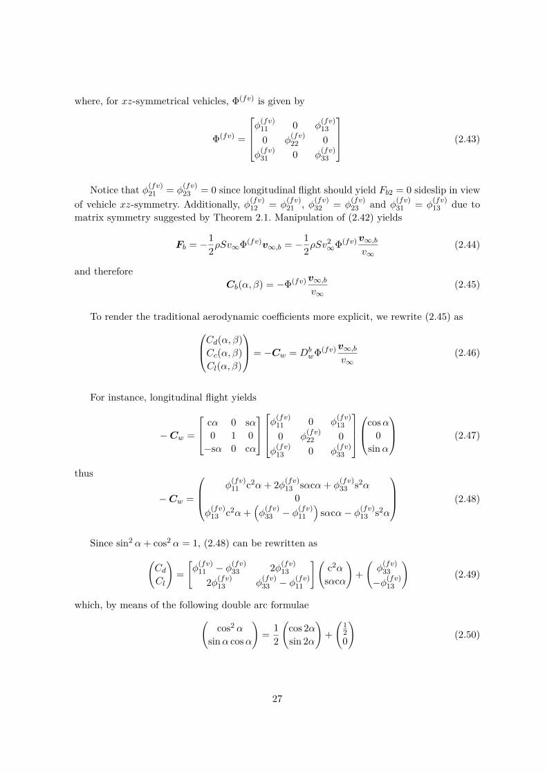
where, for xz-symmetrical vehicles, Φ(fv) is given by

Φ(fv) =

φ

(fv)11 0 φ

(fv)13

0 φ(fv)22 0

φ(fv)31 0 φ

(fv)33

(2.43)

Notice that φ(fv)21 = φ

(fv)23 = 0 since longitudinal flight should yield Fb2 = 0 sideslip in view

of vehicle xz-symmetry. Additionally, φ(fv)12 = φ

(fv)21 , φ(fv)

32 = φ(fv)23 and φ

(fv)31 = φ

(fv)13 due to

matrix symmetry suggested by Theorem 2.1. Manipulation of (2.42) yields

Fb = −12ρSv∞Φ(fv)v∞,b = −1

2ρSv2∞Φ(fv)v∞,b

v∞(2.44)

and thereforeCb(α, β) = −Φ(fv)v∞,b

v∞(2.45)

To render the traditional aerodynamic coefficients more explicit, we rewrite (2.45) asCd(α, β)Cc(α, β)Cl(α, β)

= −Cw = DbwΦ(fv)v∞,b

v∞(2.46)

For instance, longitudinal flight yields

−Cw =

cα 0 sα0 1 0−sα 0 cα

φ

(fv)11 0 φ

(fv)13

0 φ(fv)22 0

φ(fv)13 0 φ

(fv)33

cosα

0sinα

(2.47)

thus

−Cw =

φ

(fv)11 c2α+ 2φ(fv)

13 sαcα+ φ(fv)33 s2α

0φ

(fv)13 c2α+

(φ

(fv)33 − φ(fv)

11

)sαcα− φ(fv)

13 s2α

(2.48)

Since sin2 α+ cos2 α = 1, (2.48) can be rewritten as(CdCl

)=[φ

(fv)11 − φ(fv)

33 2φ(fv)13

2φ(fv)13 φ

(fv)33 − φ(fv)

11

](c2α

sαcα

)+(φ

(fv)33−φ(fv)

13

)(2.49)

which, by means of the following double arc formulae(cos2 α

sinα cosα

)= 1

2

(cos 2αsin 2α

)+(

120

)(2.50)

27

one obtains (CdCl

)= 1

2

[φ

(fv)11 − φ(fv)

33 2φ(fv)13

2φ(fv)13 φ

(fv)33 − φ(fv)

11

]︸ ︷︷ ︸

Aφ=[aφ1 aφ2]

(c2αs2α

)+ 1

2

(φ

(fv)33 + φ

(fv)11

0

)︸ ︷︷ ︸

bφ

(2.51)

Notice that (2.51) maps the unit circle to an ellipse Eφ ⊂ R2 in the (Cd, Cl) domain(double covered by α ∈ [0, 2π)). Additionally, Aφ is orthogonal with column vectors denotedby aφ1 and aφ2 (i.e., Aφ = [aφ1 aφ2]). These properties allow for direct drag polar sketchfrom inspection of Φ as Fig. 2.4 illustrates. Conversely, wind tunnel data can be identified toa φ-model by means of ellipse fitting.

Lemma 2.3If Φ � 0⇒ EΦ ⊂ R∗+ × R× R.

Démonstration. Recall from (2.46) thatCd(α, β)Cc(α, β)Cl(α, β)

= DbwΦ(fv)v∞,b

v∞(2.52)

thus

Cd(α, β) =[cαcβ sβ sαcβ

]Φ(fv)

cαcβsβsαcβ

(2.53)

Since Φ � 0, then Φ(fv) � 0 and by (2.53) one concludes that Cd(α, β) > 0 for all α, β ∈ R.

In other words, Theorem 2.1 and Lemma 2.3 state that physically meaningful drag polarsmodeled by φ-theory must reside in the right-hand side of the (Cd, Cl) domain (notice thatFig. 2.4 has inversed axes, and therefore drag polars reside in the left-hand side).

Remark 2.3Although a circular drag polar might appear overly restrictive, notice that an arbritary dragpolar can be bounded by two circles. Robustness studies might advantage from this simpleand visual approach for addressing aerodynamics uncertainties.

2.2.2 Airfoil aerodynamic derivatives

While Sec. 2.2.1 established a parallel between π-coefficients and Φ, this section presentsa connection between Φ and π-derivatives (e.g., Clp , Cmq , Cnr). Accordingly, consider a finite

28

α1Cd

Cl

bφ

aφ1

aφ2

2α1

Fw

α2Cd

Cl

bφ

aφ1

aφ2

2α2

Fw

Figure 2.4 – The elliptical drag polar concept allows for rough global qualitative visualizationof aerodynamic forces in arbitrary angles of attack. Firstly, identify bφ, aφ1 and aφ2 and sketchthe ellipse accordingly. Secondly, identify the force direction by drawing a 2α arc from aφ1(counterclockwise). The aerodynamic force Fw is parallel to the line connecting the end ofthe arc to the origin. Two examples are shown : transition and hover.

wing B immersed in an airflow of density ρ with freestream velocity v∞ at time-varying anglesof attack α(t) and sideslip β(t). Application of φ-theory yields

Mb = 12ρSB

√v2∞ + φω2

b

(Φ(mv)vb + Φ(mω)Bωb

)(2.54)

Assuming longitudinal flight and v2b >> φω2

b (a mild assumption for general aviationaircraft), (2.54) yields

Mb ≈12ρSBv∞

(Φ(mv)vb + Φ(mω)Bωb

)(2.55)

The first term is analogous to that in Sec. 2.2.1. The components of the second term (forinstance, Mb2) can be rewritten as

Mb2 = 12ρScv

2b

(c

2vb

)2φ(mω)21︸ ︷︷ ︸Cmp

P + 2φ(mω)22︸ ︷︷ ︸Cmq

Q+ 2φ(mω)23︸ ︷︷ ︸Cmr

R

(2.56)

From inspection of (2.56) one concludes that φ-theory and π-theory aerodynamic deriva-

29

tives are related according to

Φ(mω) = 12

Clp Clq ClrCmp Cmq CmrCnp Cnq Cnr

(2.57)

Remark 2.4Requiring Φ � 0 implies enforcing Φ(mω) � 0, although substitution of π-coefficients in (2.57)might result in Φ(mω) /∈ S3

++. In such case, the author suggests exploiting the closed convexcone structure of S3

++ to perform projections [Hig88] in view of the usual inner product〈X,Y 〉 = tr(XTY ).

2.2.3 Application : Thin airfoils

Classical thin symmetric airfoil theory [And10] predicts ∂Cl/∂α = 2π with associatedcenter of pressure located at a quarter-chord from the leading edge. Additionally, the pitchingmoment coefficient Cm(α) is proved to be identically zero in the center of pressure (and hencethis point is the aerodynamic center). This section illustrates φ-theory employment to thinairfoil modeling by encoding the aforementioned properties into Φ.

Firstly, differentiation of (2.51) with respect to α yields

∂

∂α

(CdCl

) ∣∣∣∣∣α=0

= 2Aφ

(− sin 2αcos 2α

) ∣∣∣∣∣α=0

=(

2φ13φ33 − φ11

)(2.58)

and thus the 2π lift slope condition imposes

φ33 = 2π + φ11 (2.59)

Furthermore, airfoil symmetry calls for ∂Cd/∂α = 0 at α = 0. Therefore

φ13 = 0 (2.60)

andφ11 = Cd0 (2.61)

where Cd0 denotes minimum drag coefficient. In summary, for symmetrical thin airfoils, wehave

Φ(fv) =

Cd0 0 00 Cy0 00 0 2π + Cd0

(2.62)

which is illustrated by the elliptical polar in Fig. 2.5. By inspection of Fig. 2.5, one concludesthat stall occurs beyond αs = 45o with associated lift coefficient Cl(αs) = π.

In the present work, cambered airfoil Φ(fv) modeling is achieved by rotation of aφ1 and

30

Cd

Cl

Cd0 + π Cd0

aφ1

aφ2

2α2αδ

Cd

Cl

Cd0 + π Cd0

π2α

v∞α

v∞α

δ

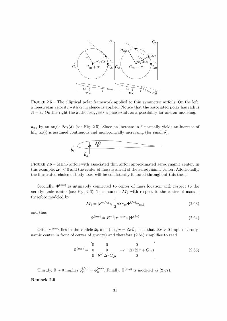
Figure 2.5 – The elliptical polar framework applied to thin symmetric airfoils. On the left,a freestream velocity with α incidence is applied. Notice that the associated polar has radiusR = π. On the right the author suggests a phase-shift as a possibility for aileron modeling.

aφ2 by an angle 2αδ(δ) (see Fig. 2.5). Since an increase in δ normally yields an increase oflift, αδ(·) is assumed continuous and monotonically increasing (for small δ).

ACb1

b3

Figure 2.6 – MH45 airfoil with associated thin airfoil approximated aerodynamic center. Inthis example, ∆r < 0 and the center of mass is ahead of the aerodynamic center. Additionally,the illustrated choice of body axes will be consistently followed throughout this thesis.

Secondly, Φ(mv) is intimately connected to center of mass location with respect to theaerodynamic center (see Fig. 2.6). The moment Mb with respect to the center of mass istherefore modeled by

Mb = [rac/cg×]12ρSv∞Φ(fv)v∞,b (2.63)

and thusΦ(mv) = B−1[rac/cg×]Φ(fv) (2.64)

Often rac/cg lies in the vehicle xb axis (i.e., r = ∆rb1 such that ∆r > 0 implies aerody-namic center in front of center of gravity) and therefore (2.64) simplifies to read

Φ(mv) =

0 0 00 0 −c−1∆r(2π + Cd0)0 b−1∆rCy0 0

(2.65)

Thirdly, Φ � 0 implies φ(fω)ij = φ

(mv)ji . Finally, Φ(mω) is modeled as (2.57).

Remark 2.5

31

The striking correlation between Φ(mv) and Φ(fω) enforces energy conservation. An accelera-ting pitching moment comes at the expense of a damping force, and vice-versa. This recipro-city sheds light on how gravity forces sustain angular periodic motion back in our falling leafexample in Sec. 2.1.3. This effect, of course, is not possible in vacuum.

2.3 Wing-propeller interaction

A common approach to modeling wing-propeller interaction is by means of the propwashinduced velocity concept [McC98]. The fundamental idea is that the velocity field v∞ isdisturbed by the propeller downstream such that its intensity |v∞| is increased while |α| and|β| are decreased. The ubiquitous approach is to resort to inviscid momentum conservationarguments, which in its integral form [And10] yields

∂

∂t

˚

V

ρv dV +‹

S(V )

(ρv · dS)v +‹

S(V )

pdS =˚

V

ρf dV (2.66)

Assuming incompressible and steady flow v, negligible body forces f , a propeller disk ofarea Sp, a control volume V around the propeller disk, freestream velocity v∞, and propwashvena contracta velocity ψ, (2.66) yields

ψψ = v∞v∞ + 1ρSp

T (2.67)

For instance, in steady hover flight (2.67) yields ψh =√T/ρSp. The square root operation

in ψh could pose problems in numerical solvers that require evaluation of ψ(T ) in T ∈ R.Additionally, vertical climb or descent yields induced velocities ψi given by [Lei06]

ψiψh

= − vcψh±

√(vcψh

)2± 1 (2.68)

where vc denotes vertical climb velocity and the signal ambiguity is dependent whether thevehicle is in descent or climb. Notice that vehicle movement added an additional complexityof signal change. Furthermore, vc/ψh > −1 yields a turbulent wake state that precludesmomentum theory employment – not even an extrapolated estimate is possible due to thedomain of definition of (2.68). Finally, extraction of induced angles of attack and sideslip from(2.67) for use in π-theory yields convoluted algebra that precludes most optimization solvers,as illustrated in the following.

32

2.3.1 π-theory wing-propeller interaction [McC98]

Traditional [McC98] aerodynamic forces and moments computation on a wing-propellerinteraction scenario requires prop-wash induced angle-of-attack αi and sideslip βi obtainedfrom ψb by solving (2.67) in the body reference frame. For this purpose, we rewrite (2.67) as

ψ

ψb1ψb2ψb3

= v2∞

cosα cosβsin β

sinα cosβ

+

TρS

00

(2.69)

Recall that, by definition, v∞,b free-stream α and β are given by

α = tan−1(v∞,b3v∞,b1

)(2.70)

andβ = sin−1

(v∞,b2v∞

)(2.71)

Accordingly, prop-wash induced αi and βi are given as function of ψ by

αi = tan−1(ψb3ψb1

)(2.72)

andβi = sin−1

(ψb2ψ

)(2.73)

Substitution of (2.69) in (2.72) and (2.73) yields

αi = tan−1(

v2∞ sinα cosβ

v2∞ cosα cosβ + T

ρS

)(2.74)

and

βi = sin−1

v2∞ sin β

4√v4∞ + 2v2

∞ cosα cosβ TρS +

(TρS

)2

(2.75)

where α and β are given by (2.70) and (2.71). Notice that, in view of convex optimizationtechniques, (2.74) and (2.75) are algebraically fairly complex.

2.3.2 φ-theory wing-propeller interaction

The aforementioned numerical issues and complexity make traditional formulation im-practicable for global TBV modeling and algorithmic control. On the other hand, φ-theoryrequires only ψψ for computation of static aerodynamic forces and moments, which is readily

33

available in (2.67). For instance, static (ωb = 0) aerodynamic forces in presence of propwashcan be modeled as

Fb = −12ρSψΦ(fv)ψ = −1

2ρSv∞Φ(fv)v∞︸ ︷︷ ︸F

(∞)b

− S

2SpΦ(fv)Tb︸ ︷︷ ︸F

(p)b

(2.76)

In sharp contrast with π-theory, (2.76) is algebraically simple, bypasses α and β, and itis defined for all T ∈ R (in fact, for all Tb ∈ R3 if non-axial propulsion forces are modeled inview of non-axial flow). Additionally, under the presented physical assumptions, (2.76) shedslight on the structural composition of Fb. Notice that Fb is composed of a superposition ofan aerodynamic force F (∞)

b due to the freestream plus an independent contribution of F (p)b

due to Tb.

Finally, notice that both π and φ-approaches employ the same physical mechanism forcomputing wing-propeller interactions. The difference is that φ-theory aerodynamic coeffi-cients algebraic restrictions yield polynomial-like equations for forces and moments computa-tion, and a globally valid superposition property as illustrated in (2.76).

2.4 Final remarks

This chapter draws the philosophical picture behind φ-theory and its basic properties. Tothe author’s best knowledge, this thesis is the first attempt to study sufficient aerodynamiccoefficients algebraic structure in view of facilitating (i) algorithmic nonlinear control designand (ii) qualitative behavior study of high maneuverable aerial vehicles. In φ-theory, wedeliberately do not pursue a more accurate description of reality. Indeed, we know for a factthat φ-theory is less accurate when compared to most other available literature. Instead, wepursue a minimal description adequate and sufficient for SOS-optimization-based guidanceand control purposes (with reasonable robustness margins). However, care was exercised tonot oversimplify reality. This thesis journey was aimed towards finding an optimal complexitypoint for modeling, and we provide a detailed validation case study in Part II to support φ-theory fitting complexity balance.

34

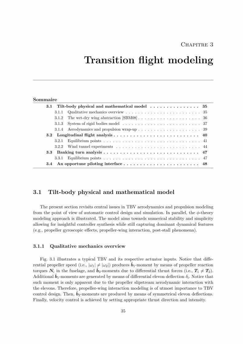
Chapitre 3

Transition flight modeling

Sommaire3.1 Tilt-body physical and mathematical model . . . . . . . . . . . . . . . 35

3.1.1 Qualitative mechanics overview . . . . . . . . . . . . . . . . . . . . . . . . 353.1.2 The wet-dry wing abstraction [SBM08] . . . . . . . . . . . . . . . . . . . . 363.1.3 System of rigid bodies model . . . . . . . . . . . . . . . . . . . . . . . . . 373.1.4 Aerodynamics and propulsion wrap-up . . . . . . . . . . . . . . . . . . . . 39

3.2 Longitudinal flight analysis . . . . . . . . . . . . . . . . . . . . . . . . . . 403.2.1 Equilibrium points . . . . . . . . . . . . . . . . . . . . . . . . . . . . . . . 413.2.2 Wind tunnel experiments . . . . . . . . . . . . . . . . . . . . . . . . . . . 44

3.3 Banking turn analysis . . . . . . . . . . . . . . . . . . . . . . . . . . . . . 473.3.1 Equilibrium points . . . . . . . . . . . . . . . . . . . . . . . . . . . . . . . 47

3.4 An opportune piloting interface . . . . . . . . . . . . . . . . . . . . . . . 48

3.1 Tilt-body physical and mathematical model

The present section revisits central issues in TBV aerodynamics and propulsion modelingfrom the point of view of automatic control design and simulation. In parallel, the φ-theorymodeling approach is illustrated. The model aims towards numerical stability and simplicityallowing for insightful controller synthesis while still capturing dominant dynamical features(e.g., propeller gyroscopic effects, propeller-wing interaction, post-stall phenomena).

3.1.1 Qualitative mechanics overview

Fig. 3.1 illustrates a typical TBV and its respective actuator inputs. Notice that diffe-rential propeller speed (i.e., |ω1| 6= |ω2|) produces b1-moment by means of propeller reactiontorques Ni in the fuselage, and b3-moments due to differential thrust forces (i.e., T1 6= T2).Additional b1-moments are generated by means of differential elevon deflection δi. Notice thatsuch moment is only apparent due to the propeller slipstream aerodynamic interaction withthe elevons. Therefore, propeller-wing interaction modeling is of utmost importance to TBVcontrol design. Then, b2-moments are produced by means of symmetrical elevon deflections.Finally, velocity control is achieved by setting appropriate thrust direction and intensity.

35

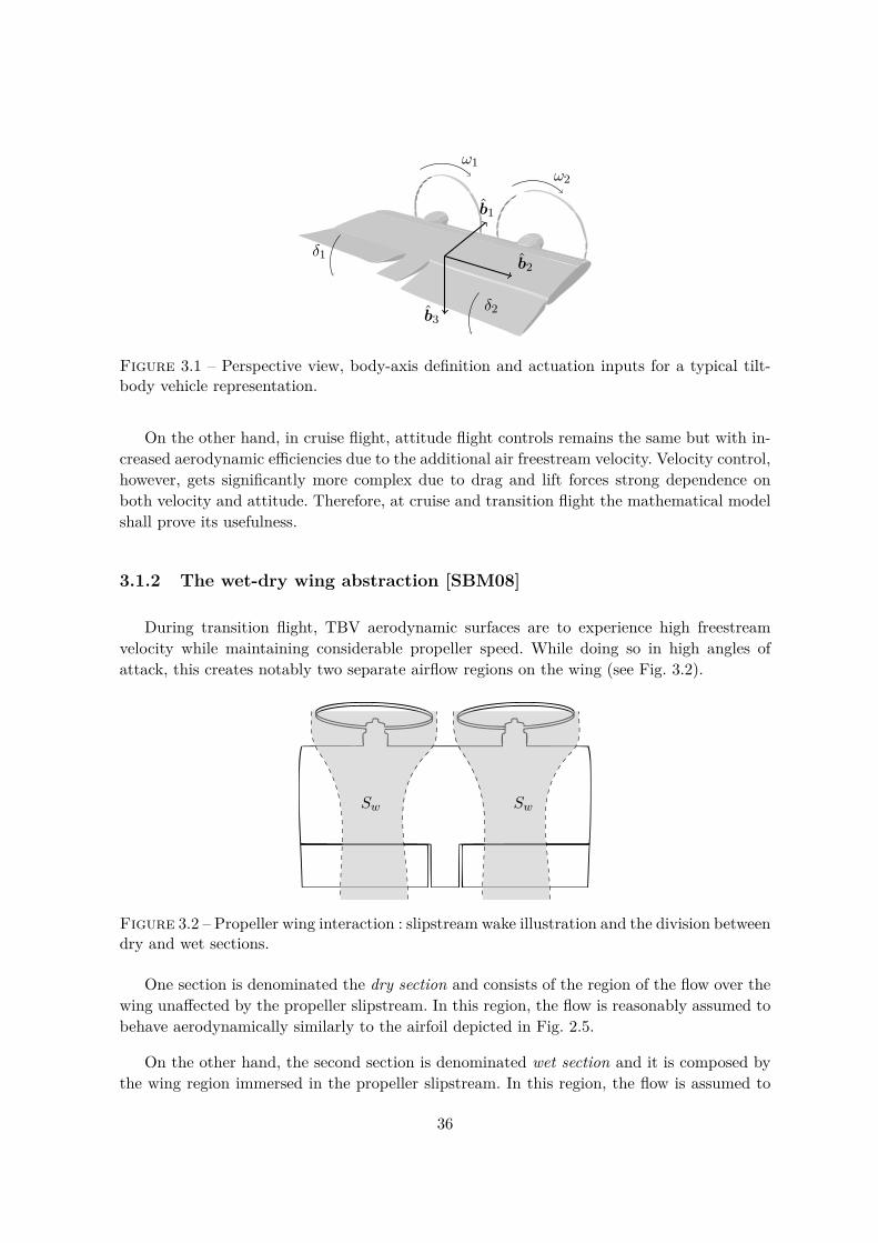
b1

b3

b2

ω2ω1

δ2

δ1

Figure 3.1 – Perspective view, body-axis definition and actuation inputs for a typical tilt-body vehicle representation.

On the other hand, in cruise flight, attitude flight controls remains the same but with in-creased aerodynamic efficiencies due to the additional air freestream velocity. Velocity control,however, gets significantly more complex due to drag and lift forces strong dependence onboth velocity and attitude. Therefore, at cruise and transition flight the mathematical modelshall prove its usefulness.

3.1.2 The wet-dry wing abstraction [SBM08]

During transition flight, TBV aerodynamic surfaces are to experience high freestreamvelocity while maintaining considerable propeller speed. While doing so in high angles ofattack, this creates notably two separate airflow regions on the wing (see Fig. 3.2).

SwSw

Figure 3.2 – Propeller wing interaction : slipstream wake illustration and the division betweendry and wet sections.

One section is denominated the dry section and consists of the region of the flow over thewing unaffected by the propeller slipstream. In this region, the flow is reasonably assumed tobehave aerodynamically similarly to the airfoil depicted in Fig. 2.5.

On the other hand, the second section is denominated wet section and it is composed bythe wing region immersed in the propeller slipstream. In this region, the flow is assumed to

36

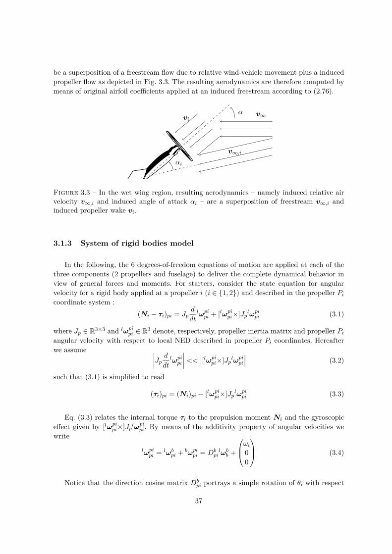
be a superposition of a freestream flow due to relative wind-vehicle movement plus a inducedpropeller flow as depicted in Fig. 3.3. The resulting aerodynamics are therefore computed bymeans of original airfoil coefficients applied at an induced freestream according to (2.76).

v∞,i

viv∞α

αi

Figure 3.3 – In the wet wing region, resulting aerodynamics – namely induced relative airvelocity v∞,i and induced angle of attack αi – are a superposition of freestream v∞,i andinduced propeller wake vi.

3.1.3 System of rigid bodies model

In the following, the 6 degrees-of-freedom equations of motion are applied at each of thethree components (2 propellers and fuselage) to deliver the complete dynamical behavior inview of general forces and moments. For starters, consider the state equation for angularvelocity for a rigid body applied at a propeller i (i ∈ {1, 2}) and described in the propeller Picoordinate system :

(Ni − τi)pi = Jpd

dtlωpipi + [lωpipi×]Jplωpipi (3.1)

where Jp ∈ R3×3 and lωpipi ∈ R3 denote, respectively, propeller inertia matrix and propeller Piangular velocity with respect to local NED described in propeller Pi coordinates. Hereafterwe assume ∣∣∣∣Jp ddt lωpipi

∣∣∣∣ << ∣∣∣[lωpipi×]Jplωpipi∣∣∣ (3.2)

such that (3.1) is simplified to read

(τi)pi = (Ni)pi − [lωpipi×]Jplωpipi (3.3)

Eq. (3.3) relates the internal torque τi to the propulsion moment Ni and the gyroscopiceffect given by [lωpipi×]Jplωpipi. By means of the additivity property of angular velocities wewrite

lωpipi = lωbpi + bωpipi = Dbpilωbb +

ωi00

(3.4)

Notice that the direction cosine matrix Dbpi portrays a simple rotation of θi with respect

37

to the b1 axis and can be written as

Dbpi(θi) =

[1 01×2

02×1 Cbpi(θi)

], Cbpi(θi) =

[cos θi sin θi− sin θi cos θi

](3.5)

Accordingly, we write each of the gyroscopic factors as

lωpipi =[

1 01×202×1 Cbpi(θi)

]PQR

+

ωi00

=

P + ωi

Cbpi

(Q

R

) (3.6)

[lωpipi×] =

0

(Q R

)Cpib

[0 1−1 0

][

0 1−1 0

]Cbpi

(Q

R

)(P + ωi)

[0 −11 0

] (3.7)

and

Jp =

Jpx 0 00 Jpn 00 0 Jpn

(3.8)

Notice that Jp is modeled as a disc hence its diagonal shape. Performing the gyroscopicproduct yields

(τi)b = (Ni)b − (P + ωi)(Jpx − Jpn)

0R

−Q

(3.9)

after an appropriate basis change. Subsequently, consider the state equation for angular ve-locity for a rigid body applied at the fuselage and described in the fuselage B coordinatesystem : ( 2∑

i=1

(Mi + τi + ppi/b × Ti + pai/b ×Ai

))b

= Jbd

dtlωbb + [lωbb×]Jblωbb (3.10)

where Ai and Ti are, respectively, aerodynamic forces in the i-wing and propeller thrust.Finally, lωbb is used to update quaternion attitude q ∈ R4 according to

dq

dt= 1

2

[0 −(lωbb)Tlωbb −[lωbb×]

]q (3.11)

The translation counterpart of the foregoing development is given by Newton’s second lawof motion applied at the fuselage yielding

mgl +Dbl

2∑i=1

(Ti +Ai) = md

dtlvbl (3.12)

38

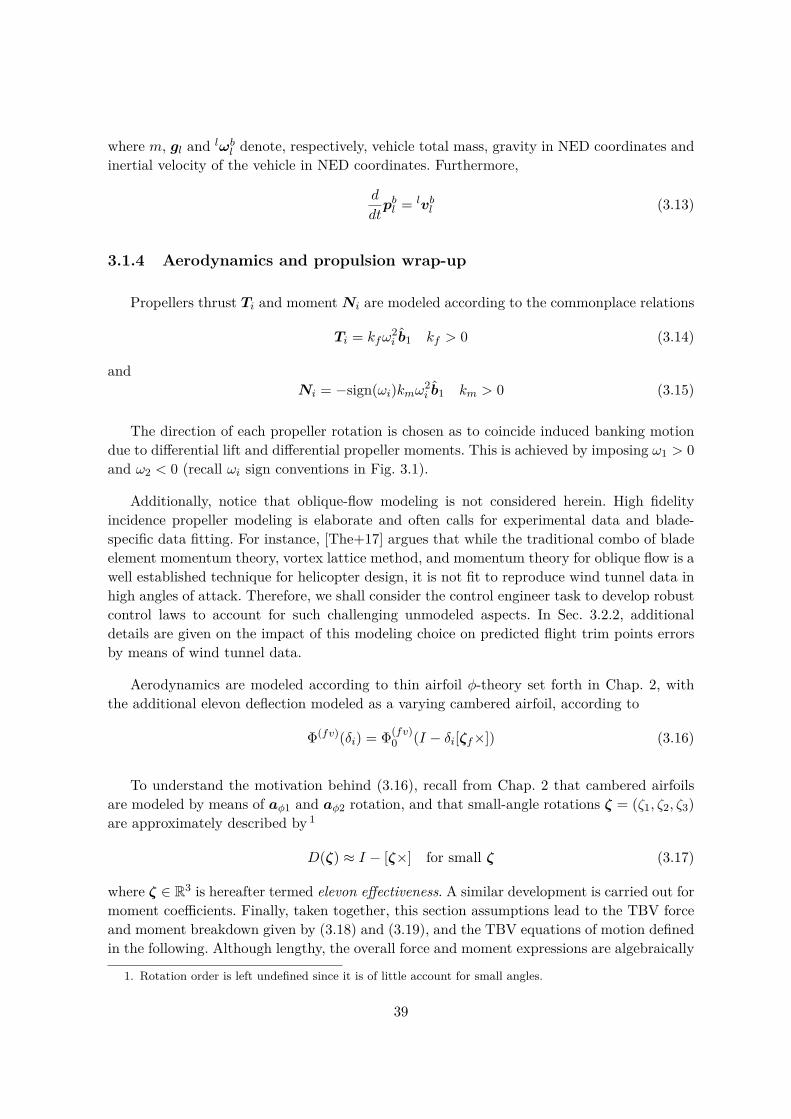
where m, gl and lωbl denote, respectively, vehicle total mass, gravity in NED coordinates andinertial velocity of the vehicle in NED coordinates. Furthermore,

d

dtpbl = lvbl (3.13)

3.1.4 Aerodynamics and propulsion wrap-up

Propellers thrust Ti and momentNi are modeled according to the commonplace relations

Ti = kfω2i b1 kf > 0 (3.14)

andNi = −sign(ωi)kmω2

i b1 km > 0 (3.15)

The direction of each propeller rotation is chosen as to coincide induced banking motiondue to differential lift and differential propeller moments. This is achieved by imposing ω1 > 0and ω2 < 0 (recall ωi sign conventions in Fig. 3.1).

Additionally, notice that oblique-flow modeling is not considered herein. High fidelityincidence propeller modeling is elaborate and often calls for experimental data and blade-specific data fitting. For instance, [The+17] argues that while the traditional combo of bladeelement momentum theory, vortex lattice method, and momentum theory for oblique flow is awell established technique for helicopter design, it is not fit to reproduce wind tunnel data inhigh angles of attack. Therefore, we shall consider the control engineer task to develop robustcontrol laws to account for such challenging unmodeled aspects. In Sec. 3.2.2, additionaldetails are given on the impact of this modeling choice on predicted flight trim points errorsby means of wind tunnel data.

Aerodynamics are modeled according to thin airfoil φ-theory set forth in Chap. 2, withthe additional elevon deflection modeled as a varying cambered airfoil, according to

Φ(fv)(δi) = Φ(fv)0 (I − δi[ζf×]) (3.16)

To understand the motivation behind (3.16), recall from Chap. 2 that cambered airfoilsare modeled by means of aφ1 and aφ2 rotation, and that small-angle rotations ζ = (ζ1, ζ2, ζ3)are approximately described by 1

D(ζ) ≈ I − [ζ×] for small ζ (3.17)

where ζ ∈ R3 is hereafter termed elevon effectiveness. A similar development is carried out formoment coefficients. Finally, taken together, this section assumptions lead to the TBV forceand moment breakdown given by (3.18) and (3.19), and the TBV equations of motion definedin the following. Although lengthy, the overall force and moment expressions are algebraically

1. Rotation order is left undefined since it is of little account for small angles.

39

simple, singularity-free and, indeed, bypass all occurrences of α and β (including propwash-induced !).

∑Fb = T1+T2−

S

4SpΦ(fv)T1−

S

4SpΦ(fv)T2−

12ρSΦ(fv)vvb+mDgl+

14ρSΦ(fv)[ζf×](δ1+δ2)vvb−

− 12ρSΦ(mv)vBωb+

S

4SpΦ(fv)[ζf×]δ1T1+ S

4SpΦ(fv)[ζf×]δ2T2+ 1

4ρSΦ(mv)[ζf×](δ1+δ2)Bvωb

(3.18)

∑Mb = −1

2ρSBΦ(mv)vvb−12ρSBΦ(mω)vBωb−

S

4SpBΦ(mv)T1−

S

4SpBΦ(mv)T2+[p1×]T1+[p2×]T2+

− S

4Sp[a1×]Φ(fv)T1−

S

4Sp[a2×]Φ(fv)T2+ S

4Sp[a1×]Φ(fv)[ζf×]δ1T1+ S

4Sp[a2×]Φ(fv)[ζf×]δ2T2+N1+N2+

+ 14ρS[a1×]Φ(fv)[ζf×]δ1vvb + 1

4ρS[a2×]Φ(fv)[ζf×]δ2vvb + 14ρS[a1×]Φ(mv)[ζf×]δ1Bvωb+

+14ρS[a2×]Φ(mv)[ζf×]δ2Bvωb+

14ρSBΦ(mv)[ζm×](δ1+δ2)vvb+

14ρSBΦ(mω)[ζm×](δ1+δ2)vBωb+

+ S

4SpBΦ(mv)[ζm×]δ1T1 + S

4SpBΦ(mv)[ζm×]δ2T2 (3.19)

Definition 3.1 (Tilt-body vehicle system)Let B be a tilt-body with inertia (m,Jb, Jp). We define a tilt-body vehicle system (TBVS) tobe the associated dynamical system given by

vb = 1m

∑Fb(x,u,w)− [ωb×]vb

ωb = J−1∑Mb(x,u,w)− J−1[ωb×]JωbDlb = −[ωb×]Dl

b

(3.20)

where∑Fb(x,u,w) and

∑Mb(x,u,w) are given by (3.18) and (3.19). Additionally, we define

x = (vb,ω, Dlb) and u = (ω1, ω2, δ1, δ2), while w ∈ R3 denotes external wind disturbance.

3.2 Longitudinal flight analysis

Longitudinal flight analysis is carried out by equilibrium point analysis (existence, unique-ness and computation results). For the present longitudinal analysis, we consider no externalwind (without loss of generality), thus the 6DOF TBV dynamical model reduction motivatesthe following definition.

Definition 3.2 (Longitudinal tilt-body system)Let B be a TBVS with inertia (m,Jb, Jp) such that

40

1. ω2(t) = −ω1(t) = ω(t)

2. δ2(t) = δ1(t) = δ(t)

3. Dlb(0) =

cos θ(0) 0 − sin θ(0)0 1 0

sin θ(0) 0 cos θ(0)

4. vb(0) =

(vb1(0) 0 vb3(0)

)T5. ωb(0) =

(0 θ(0) 0

)TWe define the longitudinal tilt-body system (LTBS) to be the simplified dynamical systemgiven by

vb1vb3

=

0 1−1 0

θvb + 1m

∑Fb(x,u)

θ = J−1yy

∑Mb2(x,u)

(3.21)

where x ∈ R4, and u ∈ R2, for the remainder of this section, such that x = (vb1, vb3, θ, θ) andu = (ω, δ).

3.2.1 Equilibrium points

We are interested in the following subset of equilibrium points of (3.21).

Definition 3.3 (Cruise points)A point (x,u) ∈ R4 × R2 is called a cruise equilibrium point if

1.∑Fb(x,u) =

∑Mb(x,u) = 0 (mechanical equilibrium condition)

2. vl3 = 0 (level flight condition)

3. θ = 0 (zero pull-up condition)

Furthermore, the set of all cruise equilibrium points is denoted Θ0 ⊂ R6.

Therefore (x,u) ∈ Θ0 if and only if∑Fb = 0∑Mb2 = 0

(3.22)

which can be rewritten as

M(θ)

v2l1

δv2l1

δT

T

= mg

sθ−cθ

0

︸ ︷︷ ︸

b(θ)

(3.23)

41

where

M(θ) =

−1

2ρSΦ(fv)(cθsθ

)12ρSΦ(fv)[ζf×]

(cθsθ

)12SSp

Φ(fv)[ζf×](

10

) (20

)− 1

2SSp

Φ(fv)(

10

)

−12ρScΦ

(mv)(cθsθ

)c2ρSΦ(mv)[ζm×]

(cθsθ

)c2SSp

Φ(mv)[ζm×](

10

)− c

2SSp

Φ(mv)(

10

)

(3.24)

Notice that we assume, without loss of generality, zero dry propwash area, i.e., Sd = 0.Furthermore, for a given θ, we decompose (3.23) into a linear system and a simpler set ofnonlinear equations such that M(θ)ξ = b(θ), ξ ∈ R4

(ξ2, ξ3) = δ(ξ1, ξ4), δ ∈ R(3.25)

The dimension of the affine linear space M(θ)ξ = b(θ) is dependent on rank (M(θ)). Thefollowing lemma is the starting point of our computation of Θ0.

Definition 3.4 (δ-inefficient angles)The set I(Φ) ⊂ R of δ-inefficient angles is defined as

I(Φ) = {θ ∈ R : Φ(mv)(

cos θsin θ

)= 0 or sin θ = 0} (3.26)

Lemma 3.1If ξm, ξf ∈ R∗ and ξm 6= ξf , then M(θ) is full rank for all θ ∈ R \ I(Φ).

Démonstration. Consider the submatrix M ′(θ) ∈ R3×3 of M(θ) consisted of the first, secondand third columns, that is,

M ′(θ) = M(θ)

1 0 00 1 00 0 10 0 0

(3.27)

Algebraic manipulation of det (M ′(θ)) yields

det(M ′(θ)

)= 1

8ρ2cS3

Sp(ζf − ζm)ζf det Φ(fv)sθΦ(mv)

(cθsθ

)(3.28)

Notice that Φ(fv) � 0 thus det Φ(fv) 6= 0. Additionally, sin θ 6= 0 and Φ(mv)(cθ sθ

)T6= 0

since θ /∈ I(Φ). Therefore, det (M ′(θ)) 6= 0 and rank (M ′(θ)) = 3. However, since M ′(θ) is asubmatrix of M(θ), then rank (M(θ)) = 3 and M(θ) is full rank.

42

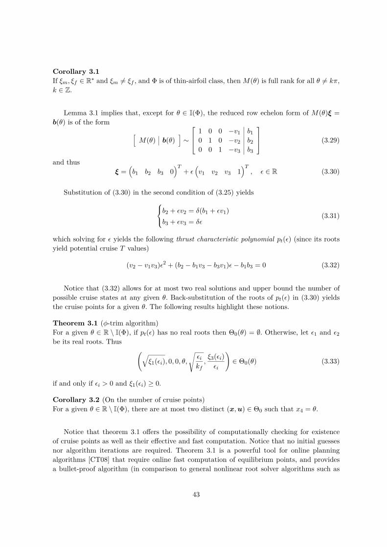
Corollary 3.1If ξm, ξf ∈ R∗ and ξm 6= ξf , and Φ is of thin-airfoil class, thenM(θ) is full rank for all θ 6= kπ,k ∈ Z.

Lemma 3.1 implies that, except for θ ∈ I(Φ), the reduced row echelon form of M(θ)ξ =b(θ) is of the form [

M(θ) b(θ)]∼

1 0 0 −v1 b10 1 0 −v2 b20 0 1 −v3 b3

(3.29)

and thusξ =

(b1 b2 b3 0

)T+ ε

(v1 v2 v3 1

)T, ε ∈ R (3.30)

Substitution of (3.30) in the second condition of (3.25) yieldsb2 + εv2 = δ(b1 + εv1)b3 + εv3 = δε

(3.31)

which solving for ε yields the following thrust characteristic polynomial pt(ε) (since its rootsyield potential cruise T values)

(v2 − v1v3)ε2 + (b2 − b1v3 − b3v1)ε− b1b3 = 0 (3.32)

Notice that (3.32) allows for at most two real solutions and upper bound the number ofpossible cruise states at any given θ. Back-substitution of the roots of pt(ε) in (3.30) yieldsthe cruise points for a given θ. The following results highlight these notions.

Theorem 3.1 (φ-trim algorithm)For a given θ ∈ R \ I(Φ), if pt(ε) has no real roots then Θ0(θ) = ∅. Otherwise, let ε1 and ε2be its real roots. Thus (√

ξ1(εi), 0, 0, θ,√εikf,ξ3(εi)εi

)∈ Θ0(θ) (3.33)

if and only if εi > 0 and ξ1(εi) ≥ 0.

Corollary 3.2 (On the number of cruise points)For a given θ ∈ R \ I(Φ), there are at most two distinct (x,u) ∈ Θ0 such that x4 = θ.

Notice that theorem 3.1 offers the possibility of computationally checking for existenceof cruise points as well as their effective and fast computation. Notice that no initial guessesnor algorithm iterations are required. Theorem 3.1 is a powerful tool for online planningalgorithms [CT08] that require online fast computation of equilibrium points, and providesa bullet-proof algorithm (in comparison to general nonlinear root solver algorithms such as

43

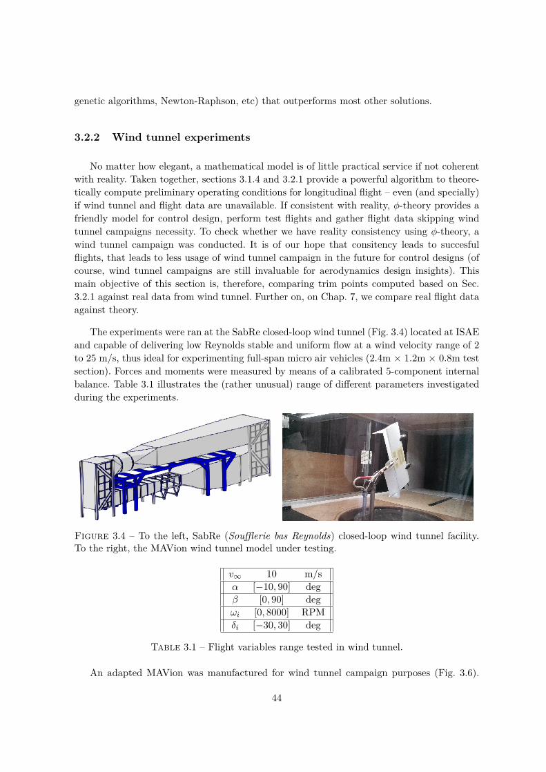
genetic algorithms, Newton-Raphson, etc) that outperforms most other solutions.

3.2.2 Wind tunnel experiments

No matter how elegant, a mathematical model is of little practical service if not coherentwith reality. Taken together, sections 3.1.4 and 3.2.1 provide a powerful algorithm to theore-tically compute preliminary operating conditions for longitudinal flight – even (and specially)if wind tunnel and flight data are unavailable. If consistent with reality, φ-theory provides afriendly model for control design, perform test flights and gather flight data skipping windtunnel campaigns necessity. To check whether we have reality consistency using φ-theory, awind tunnel campaign was conducted. It is of our hope that consitency leads to succesfulflights, that leads to less usage of wind tunnel campaign in the future for control designs (ofcourse, wind tunnel campaigns are still invaluable for aerodynamics design insights). Thismain objective of this section is, therefore, comparing trim points computed based on Sec.3.2.1 against real data from wind tunnel. Further on, on Chap. 7, we compare real flight dataagainst theory.

The experiments were ran at the SabRe closed-loop wind tunnel (Fig. 3.4) located at ISAEand capable of delivering low Reynolds stable and uniform flow at a wind velocity range of 2to 25 m/s, thus ideal for experimenting full-span micro air vehicles (2.4m × 1.2m × 0.8m testsection). Forces and moments were measured by means of a calibrated 5-component internalbalance. Table 3.1 illustrates the (rather unusual) range of different parameters investigatedduring the experiments.

Figure 3.4 – To the left, SabRe (Soufflerie bas Reynolds) closed-loop wind tunnel facility.To the right, the MAVion wind tunnel model under testing.

v∞ 10 m/sα [−10, 90] degβ [0, 90] degωi [0, 8000] RPMδi [−30, 30] deg

Table 3.1 – Flight variables range tested in wind tunnel.

An adapted MAVion was manufactured for wind tunnel campaign purposes (Fig. 3.6).

44

Its main objectives were to enable rigid installment of the internal balance in both configu-rations and to provide a non-deformable airfoil section to aerodynamic identification. Fig.3.5 illustrates the electronic counterpart. Notice that elevon deflections were measured bymeans of potentiometers installed directly at the elevons avoiding servo measurements thatare susceptible to inaccuracy due to rod deformations and servo-control errors. On the otherhand, propellers speed were measured by the brushless CC motors speed controllers.

1

2

3

ARM7 µCXbeeω2

δ2,command

δ2

Figure 3.5 – MAVion wind tunnel model instrumentation.

1

2 34 5 6 7

Xbee

ωt V∞

Fb,Mb

α

ω, δ

Figure 3.6 – Wind tunnel acquisition system set-up.

The supporting structure was mounted beforehand and forces and moments were mea-sured to determine parasite effects. The data set comprises of wind relative velocity, elevondeflection and propeller rotation required to achieve static equilibrium in a given angle ofattack. The experimental procedure fundamental idea is to, as previously done in [Ita+01],for each sampled α, iteratively search for values V∞, ωi, δi (in that order) that will deliver ae-rodynamic/propulsion forces and moments (notice gravitational suppression) that will cancelgravitational forces and moments on the flying model ; which has a different mass distributionthan the wind tunnel model that is not meant to fly. More precisely, for a given α, v∞ wasexperimentally chosen as to set lift equal flying prototype weight (i.e., the real flying proto-type, in opposition to the wind tunnel model, which has a different weight). Next, ω1 and ω2

45

were chosen to balance out drag forces. Then, δ1 and δ2 were changed until pitching momentwas eliminated. However, modifying any of these three control variables resulted in a changeof all balance measurements. Therefore, multiple iterations of this process proceeded until areasonable fixed measurement was found. The desired flying model mass distribution is suchthat the center of mass is longitudinally located at a position 0.15c away from the leadingedge and is motivated by a 10% stability margin controls requirement. The results can beseen in Fig. 3.7 along with power required curves.

0 10 20 30 40 50 60 70 80 900

10

20

30

v l1(m

/s)

φ-TheoryWind Tunnel

0 10 20 30 40 50 60 70 80 90

600

800

ω(rad

/s)

φ-TheoryWind Tunnel

0 10 20 30 40 50 60 70 80 90−30

−20

−10

0

θ (deg)

δ(deg)

φ-TheoryWind Tunnel

Figure 3.7 – Longitudinal cruise points for a given test vehicle.

The results validate the design experimentally demonstrating that the MAVion is capableof sustaining flight from 0m/s to 20m/s in the absence of wind. Equivalently speaking, theMAVion is capable of maintaining hover flight in adverse wind conditions up to 20m/s (seeFig. 3.8). It is noted that MAVion maximum speed was not reached in wind tunnel testing dueto internal balance strain gauge saturation and it is still an unknown. However, the blow-upin propeller engine rotation ω for small angles of attack in the equilibrium figures suggestsan upper bound of vn ≤ 20m/s. Finally, the elevator deflection angle shows a maximum ofδ = 27o at α = 40o, within the range of the elevon aerodynamic efficiency. This confirms thatthe propeller slipstream is strong enough to guarantee pitch control throughout the entire

46

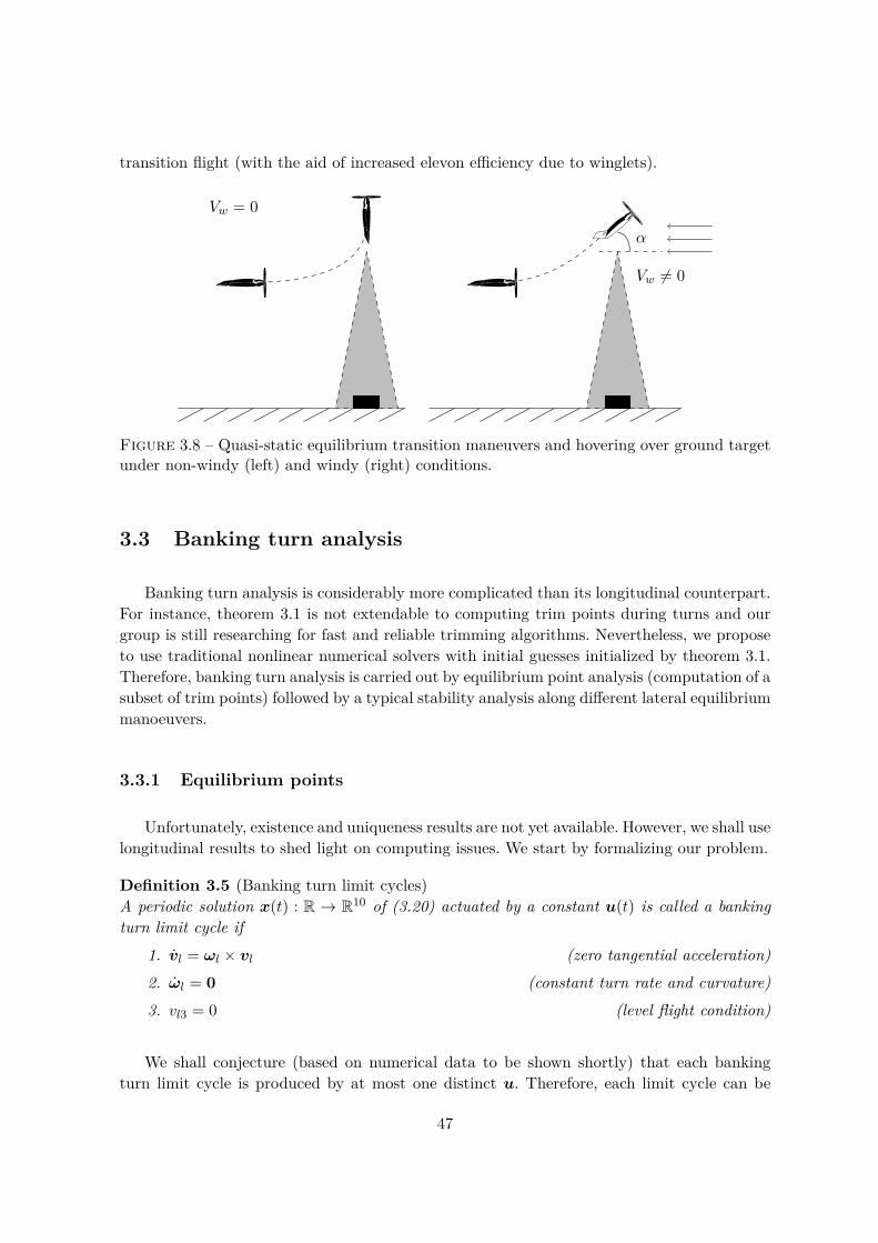
transition flight (with the aid of increased elevon efficiency due to winglets).

Vw = 0

α

Vw 6= 0

Figure 3.8 – Quasi-static equilibrium transition maneuvers and hovering over ground targetunder non-windy (left) and windy (right) conditions.

3.3 Banking turn analysis

Banking turn analysis is considerably more complicated than its longitudinal counterpart.For instance, theorem 3.1 is not extendable to computing trim points during turns and ourgroup is still researching for fast and reliable trimming algorithms. Nevertheless, we proposeto use traditional nonlinear numerical solvers with initial guesses initialized by theorem 3.1.Therefore, banking turn analysis is carried out by equilibrium point analysis (computation of asubset of trim points) followed by a typical stability analysis along different lateral equilibriummanoeuvers.

3.3.1 Equilibrium points

Unfortunately, existence and uniqueness results are not yet available. However, we shall uselongitudinal results to shed light on computing issues. We start by formalizing our problem.

Definition 3.5 (Banking turn limit cycles)A periodic solution x(t) : R → R10 of (3.20) actuated by a constant u(t) is called a bankingturn limit cycle if

1. vl = ωl × vl (zero tangential acceleration)2. ωl = 0 (constant turn rate and curvature)3. vl3 = 0 (level flight condition)

We shall conjecture (based on numerical data to be shown shortly) that each bankingturn limit cycle is produced by at most one distinct u. Therefore, each limit cycle can be

47

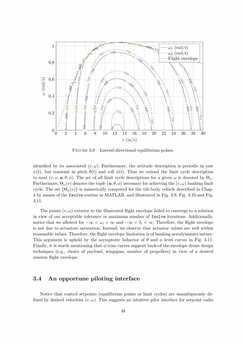
0 2 4 6 8 10 12 14 16 18 20 22 24 26 28 300

0,2

0,4

0,6

0,8

1−

850

−850

−850

−850−850

−850

−85

0

−85

0−

850

−800

−800

−800

−800−800

−800

−80

0−

800

−700

−700

−700

−700

−70

0

−70

0−

700

−600

−600−600

−60

0

−550

−550

−55

0

−51

0510

550

550

550600

600

600

600

600

700

700

700700

700

700700

800

800

800

800 800

800800

800850

85085

0

850 850

850

850

850850

v (m/s)

ω(rad

/s)

ω1 (rad/s)ω2 (rad/s)Flight envelope

Figure 3.9 – Lateral-directional equilibrium polars.

identified by its associated (v, ω). Furthermore, the attitude description is periodic in yawψ(t), but constant in pitch θ(t) and roll φ(t). Thus we extend the limit cycle descriptionto read (v, ω,u, θ, φ). The set of all limit cycle descriptions for a given ω is denoted by Θω.Furthermore, Θω(v) denotes the tuple (u, θ, φ) necessary for achieving the (v, ω) banking limitcycle. The set {Θω(v)} is numerically computed for the tilt-body vehicle described in Chap.4 by means of the fsolve routine in MATLAB, and illustrated in Fig. 3.9, Fig. 3.10 and Fig.3.11.

The points (v, ω) exterior to the illustrated flight envelope failed to converge to a solutionin view of our acceptable tolerance or maximum number of fsolve iterations. Additionally,notice that we allowed for −∞ < ωi < ∞ and −∞ < δi < ∞. Therefore, the flight envelopeis not due to actuators saturation. Instead, we observe that actuator values are well withinreasonable values. Therefore, the flight envelope limitation is of banking aerodynamics nature.This argument is upheld by the asymptotic behavior of θ and φ level curves in Fig. 3.11.Finally, it is worth mentioning that φ-trim curves support back-of-the-envelope drone designtechniques (e.g., choice of payload, wingspan, number of propellers) in view of a desiredmission flight envelope.

3.4 An opportune piloting interface

Notice that control setpoints (equilibrium points or limit cycles) are unambiguously de-fined by desired velocities (v, ω). This suggests an intuitive pilot interface for setpoint radio

48

0 2 4 6 8 10 12 14 16 18 20 22 24 26 28 300

0,2

0,4

0,6

0,8

1

−30

−30

−30

−30

−30

−30

−30

−30

−25

−25

−25

−25

−25

−25

−25

−25

−20

−20

−20

−20 −20−20

−20

−20

−20

−20

−10

−10

−10

−10−10

−10

−10

−10

−10

v (m/s)

ω(rad

/s)

δ1 (deg)δ2 (deg)Flight envelope

Figure 3.10 – Lateral-directional equilibrium polars.

control (RC) where the pilot controls the TBV thinking on where it needs to go insteadof which orientation it needs to be. This abstracts the internal workings of the drone, re-lieves piloting efforts and provides ground for straightforward automatic guidance laws. Fig.3.12 illustrates our proposition of RC controller input assignment for commonplace RC radiostandards.

An equivalent piloting approach to tilt-wing vehicles is heuristically defined in [HMM17].We support this line of thought by providing the aforementioned theoretical results.

49

0 2 4 6 8 10 12 14 16 18 20 22 24 26 28 300

0,2

0,4

0,6

0,8

1

20

20

2020 20

4040

40

4040

4060

60

60

6060

60

60

80

80

80

8080

80

80

9090

90

90

90

90

90

9090

90

0 0 0 0 0 0 0 0 0 0 0 0 0 0 0 0 0

00

020

2020

20

20

20

2020 20

4040

40

40

40

40

40

40

4040

6060

60

60

60

60

6060

60

60

60

v (m/s)

ω(rad

/s)

θ (deg)φ (deg)Flight envelope

Figure 3.11 – Lateral-directional equilibrium polars.

Vx

ψ

Vz

Vy

Vx

ψ

Vz

Vy

Mode 1 Mode 2

Figure 3.12 – Input assignments of standard RC radio modes. Notice that ψ, Vx, Vz andVy denote, respectively, desired heading with respect to geographic North, forward velocity,vertical velocity and lateral velocity.

50

Part II

An autopilot design case study and flighttesting

51

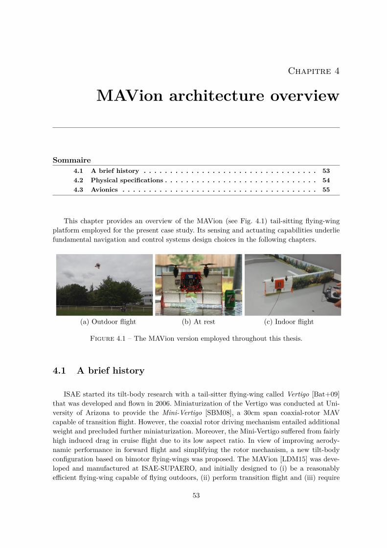
Chapitre 4

MAVion architecture overview

Sommaire4.1 A brief history . . . . . . . . . . . . . . . . . . . . . . . . . . . . . . . . . 534.2 Physical specifications . . . . . . . . . . . . . . . . . . . . . . . . . . . . . 544.3 Avionics . . . . . . . . . . . . . . . . . . . . . . . . . . . . . . . . . . . . . 55

This chapter provides an overview of the MAVion (see Fig. 4.1) tail-sitting flying-wingplatform employed for the present case study. Its sensing and actuating capabilities underliefundamental navigation and control systems design choices in the following chapters.

(a) Outdoor flight (b) At rest (c) Indoor flight

Figure 4.1 – The MAVion version employed throughout this thesis.

4.1 A brief history

ISAE started its tilt-body research with a tail-sitter flying-wing called Vertigo [Bat+09]that was developed and flown in 2006. Miniaturization of the Vertigo was conducted at Uni-versity of Arizona to provide the Mini-Vertigo [SBM08], a 30cm span coaxial-rotor MAVcapable of transition flight. However, the coaxial rotor driving mechanism entailed additionalweight and precluded further miniaturization. Moreover, the Mini-Vertigo suffered from fairlyhigh induced drag in cruise flight due to its low aspect ratio. In view of improving aerody-namic performance in forward flight and simplifying the rotor mechanism, a new tilt-bodyconfiguration based on bimotor flying-wings was proposed. The MAVion [LDM15] was deve-loped and manufactured at ISAE-SUPAERO, and initially designed to (i) be a reasonablyefficient flying-wing capable of flying outdoors, (ii) perform transition flight and (iii) require

53

a minimum number of moving parts (e.g., no tilting wings, no tilting motors). The main de-sign guidelines were simplicity – from the manufacturing point of view – and transition flightcapability. In parallel, a Roll and Fly [Alh+16] version with wheels was designed to pursuepredominantly indoor exploration missions. The latter is not pursued in this thesis althoughall but a few results are applicable.

4.2 Physical specifications

The MAVion is designed for simultaneous outdoor and indoor missions in complex en-vironments. It should be small enough to perform building intrusion but large enough forreasonable endurance. Our most recent version has 420g (complete airframe, with avionicsand batteries, see Table 4.1), 210mm chord and 420mm wingspan (thus aspect ratio AR = 2).The elevons correspond to 33% of its MH45 profile chord (see Fig. 4.2) and it possesses win-glets for enhanced lateral stability during initial flight tests. After control law validation, thewinglets could be removed for reduced drag and increased maneuverability. In fact, wingletsare not required for stable operation at any speed – i.e., from zero (hover) to cruise flightspeed – if lateral instability is accounted for in automatic control design.

210

420175

177.8

70

Figure 4.2 – MAVion physical dimensions in mm (without winglets).

APC 7×5 propellers are employed and powered by AXi 2204/54 brushless motors (de-signed for indoor aerobatic models). Motor power electronics is handled by a customizedelectronic speed control systems (ESC) based on Mikrokopter 1 boards. As one would ima-gine, the choice of propeller geometry is dependent on mission hover/cruise quotient. It isworth mentioning that recent studies [Pen+13] conducted at ISAE exploits passive twist

1. Mikrokopter BL-Ctrl I2C ESC. For more information, please visithttp://www.mikrokopter.de/en/home.

54

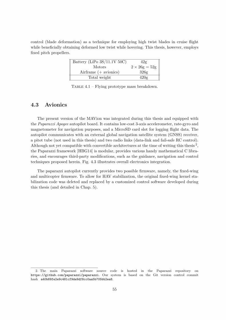
control (blade deformation) as a technique for employing high twist blades in cruise flightwhile beneficially obtaining deformed low twist while hovering. This thesis, however, employsfixed pitch propellers.

Battery (LiPo 3S/11.1V 50C) 42gMotors 2× 26g = 52g

Airframe (+ avionics) 326gTotal weight 420g

Table 4.1 – Flying prototype mass breakdown.

4.3 Avionics

The present version of the MAVion was integrated during this thesis and equipped withthe Paparazzi Apogee autopilot board. It contains low-cost 3-axis accelerometer, rate-gyro andmagnetometer for navigation purposes, and a MicroSD card slot for logging flight data. Theautopilot communicates with an external global navigation satellite system (GNSS) receiver,a pitot tube (not used in this thesis) and two radio links (data-link and fail-safe RC control).Although not yet compatible with convertible architectures at the time of writing this thesis 2,the Paparazzi framework [HBG14] is modular, provides various handy mathematical C libra-ries, and encourages third-party modifications, such as the guidance, navigation and controltechniques proposed herein. Fig. 4.3 illustrates overall electronics integration.

The paparazzi autopilot currently provides two possible firmware, namely, the fixed-wingand multicopter firmware. To allow for HAV stabilization, the original fixed-wing kernel sta-bilization code was deleted and replaced by a customized control software developed duringthis thesis (and detailed in Chap. 5).

2. The main Paparazzi software source code is hosted in the Paparazzi repository onhttps://github.com/paparazzi/paparazzi. Our system is based on the Git version control commithash a40b69fe2e9c481cf9de9df8cc0aa5b705bb2ea8.

55

Magnetometer

IMUARM

I2C

I2C

GNSS receiver

Pitot tube

RC radio

Telemetry radio

Elevons Potentiometers

ESC1

ESC2

DC motor 1

DC motor 2

Servo 1

Servo 2

Apogee board

I2C

PPM

UART

ADC

UART

I2CI2CPWMPWM

Figure 4.3 – MAVion avionics integration architecture.

56

Chapitre 5

Control system design

While still in the early phases of autopilot design, engineers often face the ever-presentdilemma of how control authority should be shared between computers and humans – espe-cially in inherently unstable vehicles, where manual piloting is dull and demanding. In thiscase study, we pursue a control architecture that could be used to service either human pilots,high level guidance loops or planning algorithms. This chapter exploits previous chapters re-sults to propose a relatively natural solution to the control problem with a fitting share ofresponsibilities between human and machine.

Sommaire5.1 Introduction . . . . . . . . . . . . . . . . . . . . . . . . . . . . . . . . . . 575.2 The region-of-attraction-based gain-scheduling approach . . . . . . . . 595.3 The feasibility issue in RoA-GS – a case study . . . . . . . . . . . . . . 62

5.3.1 Nonlinear controllability and underactuation analysis . . . . . . . . . . . . 645.3.2 Linear quadratic regulator (LQR) design . . . . . . . . . . . . . . . . . . . 655.3.3 Region-of-attraction computation . . . . . . . . . . . . . . . . . . . . . . . 66

5.4 The quaternion uncontrollable linearized dynamics conundrum . . . . 695.4.1 Quaternion attitude dynamics . . . . . . . . . . . . . . . . . . . . . . . . . 695.4.2 The time-invariant linear quadratic regulator . . . . . . . . . . . . . . . . 725.4.3 The reduced quaternion model revisited . . . . . . . . . . . . . . . . . . . 735.4.4 The virtual stabilizing input solution . . . . . . . . . . . . . . . . . . . . . 765.4.5 The mixed parametrization solution . . . . . . . . . . . . . . . . . . . . . 79

5.5 The MAVion control architecture . . . . . . . . . . . . . . . . . . . . . . 795.6 Simulation investigation . . . . . . . . . . . . . . . . . . . . . . . . . . . 80

5.6.1 Simulation setup . . . . . . . . . . . . . . . . . . . . . . . . . . . . . . . . 805.6.2 Simulation results . . . . . . . . . . . . . . . . . . . . . . . . . . . . . . . 81

5.7 Closing remarks . . . . . . . . . . . . . . . . . . . . . . . . . . . . . . . . 82

5.1 Introduction

The highly nonlinear nature of tail-sitting transitioning flight precludes direct applicationof traditional linear control theory and calls for more general techniques. Feedback lineariza-tion methods, for instance, render a nonlinear system linear by means of appropriate state

57

diffeomorphism transformations. However, such transformation exists only for fully actuatedsystems (generally absent in aerial robotics) and, additionally, controller design is often chal-lenging due to unstable zero dynamics. Sliding mode control, on the other hand, applies tounderactuated systems but model uncertainties may lead to excessive chattering and excita-tion of unmodeled dynamics. Advances in computing hardware and optimization theory allowfor successful model predictive control design but its non-convex nature poses challenges forhigh dimensional embedded real-time applications.

Gain-scheduling techniques, on the other hand, are based on linearization of nonlinearsystems at desired operating points thus profiting of well established and computationallyinexpensive linear control techniques. The manual sequential controller design and tuningare tedious but have being increasingly replaced by H∞-based automated algorithms [GA11].Furthermore, advances in regions-of-attraction inner estimates by means of direct computationof Lyapunov functions using sum-of-squares (SOS) optimization [Joh00] ; [Par00] allow forefficient stability guarantees while switching scheduled controllers. This regions-of-attraction-based gain scheduling (RoA-GS) strategy was recently validated in agile fixed-wing vehicles[MCT14] and promoted to a motion planning technique by means of a sparse randomized treeof scheduled linear quadratic regulators (LQR) [Ted+10].

The present chapter contributes to the RoA-GS framework by investigating whether theRoA-GS planning technique always yield a finite (or even countable infinite) sequence ofcontrollers leading to a desired set-point given a well-posed controllable nonlinear system anda reference equilibrium trajectory. Sec. 5.2 revisits the RoA-GS method and sets up notation.Sec. 5.3 proposes a well-posed nonlinear system that is globally controllable and fully-actuatedalmost everywhere, but RoA-GS fails to track a given equilibrium trajectory. Fortunately, thatis not the case with tail-sitting transitioning flight, as previously demonstrated in [LDM15].

Among the diverse attitude parametrization philosophies existent in the literature, qua-ternion algebra stands out due to its simplicity and uniform numerical stable appliance inSO(3) in sharp contrast to Euler angles that possess singularities that preclude their globalemployment and calls for local charts switching that increases system complexity. Further-more, an increasing use of quaternion algebra in the field of unmanned aerial vehicles (UAV)is apparent as atmospheric vehicles become more acrobatic [CCS13] and/or allow for multipleflight modes [LDM15].

On the control systems counterpart, undemanding control laws are available for qua-ternion attitude control in both linear and nonlinear worlds. For instance, previous work[WD91] obtained globally exponentially stable proportional-derivative control laws by meansof energy-based Lyapunov functions for the rigid-body tracking problem. Central drawbacksthat arrive, namely, quaternion unwinding (due to double cover of SO(3)) and chattering(due to measurement noise), can be efficiently handled by hysteresis mechanisms [MST11].However, we restate that the aforementioned techniques require fully-actuated systems.

Linear techniques, on the other hand, are well-established and capable of dealing withplant uncertainties and nonlinearities by means of linearization over a trajectory and gainscheduling. Linear Quadratic Control (LQR)-based attitude controllers are often applied due

58

to its intuitive tuning process and reasonable stability robustness properties. Furthermore,LQR scales and integrates well in underactuated systems planning algorithms [MT12]. Al-though unwinding can be handled by path-lifting techniques [MST13], nonlinear quaterniondifferential equations of motion linearization yields non-stabilizable systems that precludeLQR techniques employment. Previous work on spacecraft [Yan16] and UAV [Val+13] atti-tude control resort to a reduced quaternion model where only three out of four quaternioncoordinates are exploited. Moreover, the latter proves global stability and local optimality ofthe proposed approach.

The present chapter draws a numerical stability figure of merit of the optimal solution ofthe LQR problem for the aforementioned reduced quaternion model and presents its nume-rically unstable regions. Additionally, we propose three methods to obtain well-posed LQRproblems over all operating points. The first is based on the reduced quaternion model withan appropriate change of coordinates. The second is to append a virtual stabilizing input(VSI) to the nonlinear system to attain controllable linearized systems. The VSI directionshould be appropriately chosen to not disturb the controllable modes of the system. Thethird is the classical approach of setting local Euler angle maps on top of a global quater-nion description. Finally, we show that a class of constant angular velocity tracking problemsare time-invariant under an appropriate change of variables such that time-invariant LQRtechniques are applicable.

The quaternion LQR section layout is as follows : Sec. 5.4.1 presents the quaternionnotation employed herein and reviews the pertinent linearized quaternion dynamics propertieswhile presenting the key coordinate transformation of the present work. Sec. 5.4.2 reviews therelevant LQR concepts and presents a numerical stability figure of merit for the associatedalgebraic Riccati equation. Secs. 5.4.3 and 5.4.4 derive the two proposed methods for linearizedquaternion attitude LQR control design.

The aforementioned general theoretical points come together to support the MAVioncontrol architecture described in Sec. 5.5. Simulations were conducted to validate the controllaws and are described in Sec. 5.6. Finally, Sec. 5.7 presents opportunities for future work andclosing remarks.

5.2 The region-of-attraction-based gain-scheduling approach

Consider a nonlinear globally controllable dynamical system f ∈ C∞ of the form

dx

dt= f(x,u) (5.1)

where x ∈ Rn and u ∈ Rm are, respectively, state-space coordinates and control inputs.Furthermore, consider a given equilibrium point (x0,u0), i.e.,

f(x0,u0) = 0 (5.2)

59

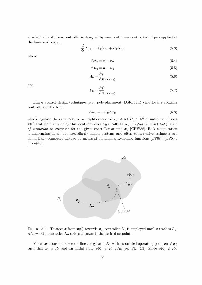
at which a local linear controller is designed by means of linear control techniques applied atthe linearized system

d

dt∆x0 = A0∆x0 +B0∆u0 (5.3)

where∆x0 = x− x0 (5.4)

∆u0 = u− u0 (5.5)

A0 = ∂f

∂x

∣∣∣(x0,u0)

(5.6)

andB0 = ∂f

∂u

∣∣∣(x0,u0)

(5.7)

Linear control design techniques (e.g., pole-placement, LQR, H∞) yield local stabilizingcontrollers of the form

∆u0 = −K0∆x0 (5.8)

which regulate the error ∆x0 on a neighborhood of x0. A set R0 ⊂ Rn of initial conditionsx(0) that are regulated by this local controller K0 is called a region-of-attraction (RoA), basinof attraction or attractor for the given controller around x0 [CHW88]. RoA computationis challenging in all but exceedingly simple systems and often conservative estimates arenumerically computed instead by means of polynomial Lyapunov functions [TP08] ; [TP09] ;[Top+10].

R0

R1

x0

x1

x(0)

Switch!K0

K1

Figure 5.1 – To steer x from x(0) towards x0, controller K1 is employed until x reaches R0.Afterwards, controller K0 drives x towards the desired setpoint.

Moreover, consider a second linear regulator K1 with associated operating point x1 6= x0such that x1 ∈ R0 and an initial state x(0) ∈ R1 \ R0 (see Fig. 5.1). Since x(0) /∈ R0,

60

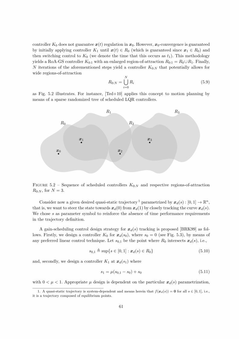
controllerK0 does not guarantee x(t) regulation in x0. However, x0-convergence is guaranteedby initially applying controller K1 until x(t) ∈ R0 (which is guaranteed since x1 ∈ R0) andthen switching control to K0 (we denote the time that this occurs as t1). This methodologyyields a RoA-GS controller K0:1 with an enlarged region-of-attraction R0:1 = R0∪R1. Finally,N iterations of the aforementioned steps yield a controller K0:N that potentially allows forwide regions-of-attraction

R0:N =N⋃i=0

Ri (5.9)

as Fig. 5.2 illustrates. For instance, [Ted+10] applies this concept to motion planning bymeans of a sparse randomized tree of scheduled LQR controllers.

R0

x0

R1

x1

R2

x2

R3

x3

Figure 5.2 – Sequence of scheduled controllers K0:N and respective regions-of-attractionR0:N , for N = 3.

Consider now a given desired quasi-static trajectory 1 parametrized by xd(s) : [0, 1]→ Rn,that is, we want to steer the state towards xd(0) from xd(1) by closely tracking the curve xd(s).We chose s as parameter symbol to reinforce the absence of time performance requirementsin the trajectory definition.

A gain-scheduling control design strategy for xd(s) tracking is proposed [BRK99] as fol-lows. Firstly, we design a controller K0 for xd(s0), where s0 = 0 (see Fig. 5.3), by means ofany preferred linear control technique. Let s0,1 be the point where R0 intersects xd(s), i.e.,

s0,1 , sup{s ∈ [0, 1] : xd(s) ∈ R0} (5.10)

and, secondly, we design a controller K1 at xd(s1) where

s1 = µ(s0,1 − s0) + s0 (5.11)

with 0 < µ < 1. Appropriate µ design is dependent on the particular xd(s) parametrization,

1. A quasi-static trajectory is system-dependent and means herein that f(xd(s)) = 0 for all s ∈ [0, 1], i.e.,it is a trajectory composed of equilibrium points.

61

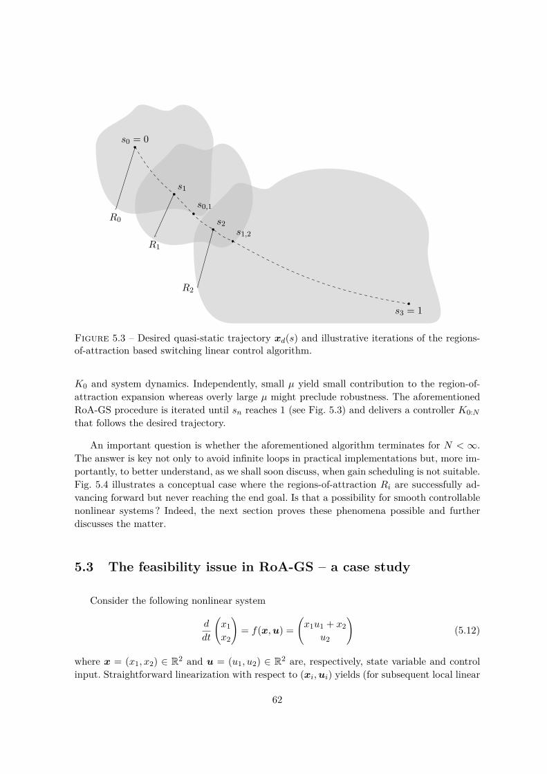
R0

R1

R2

s0 = 0

s1

s0,1

s2s1,2

s3 = 1

Figure 5.3 – Desired quasi-static trajectory xd(s) and illustrative iterations of the regions-of-attraction based switching linear control algorithm.

K0 and system dynamics. Independently, small µ yield small contribution to the region-of-attraction expansion whereas overly large µ might preclude robustness. The aforementionedRoA-GS procedure is iterated until sn reaches 1 (see Fig. 5.3) and delivers a controller K0:Nthat follows the desired trajectory.

An important question is whether the aforementioned algorithm terminates for N < ∞.The answer is key not only to avoid infinite loops in practical implementations but, more im-portantly, to better understand, as we shall soon discuss, when gain scheduling is not suitable.Fig. 5.4 illustrates a conceptual case where the regions-of-attraction Ri are successfully ad-vancing forward but never reaching the end goal. Is that a possibility for smooth controllablenonlinear systems ? Indeed, the next section proves these phenomena possible and furtherdiscusses the matter.

5.3 The feasibility issue in RoA-GS – a case study

Consider the following nonlinear system

d

dt

(x1x2

)= f(x,u) =

(x1u1 + x2

u2

)(5.12)

where x = (x1, x2) ∈ R2 and u = (u1, u2) ∈ R2 are, respectively, state variable and controlinput. Straightforward linearization with respect to (xi,ui) yields (for subsequent local linear

62

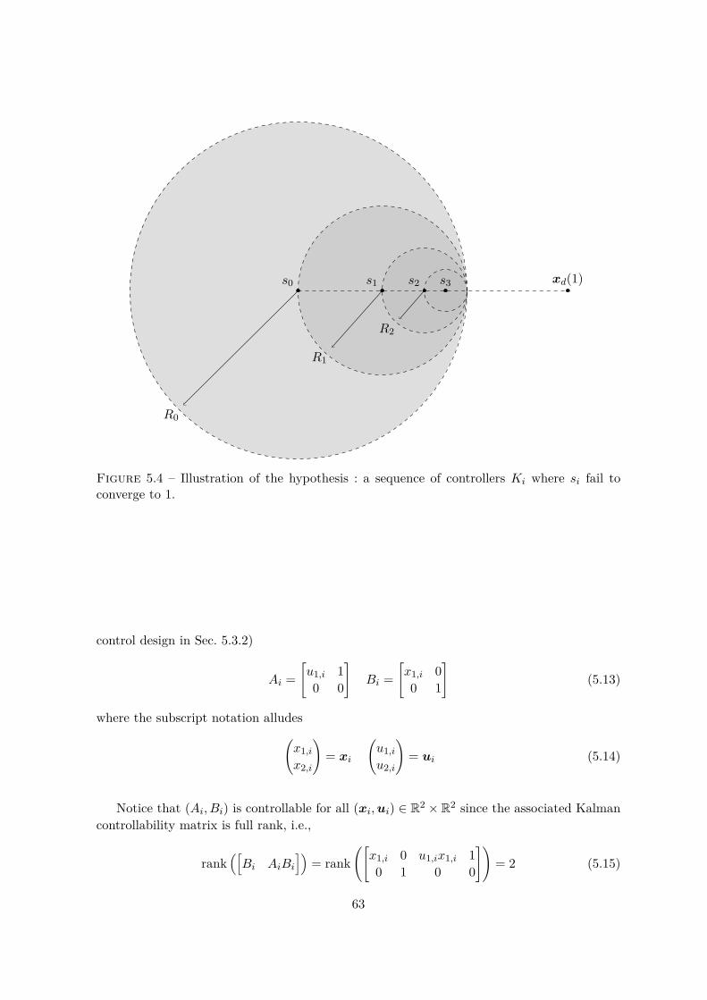
s0 s1 s2 s3 xd(1)

R0

R1

R2

Figure 5.4 – Illustration of the hypothesis : a sequence of controllers Ki where si fail toconverge to 1.

control design in Sec. 5.3.2)

Ai =[u1,i 10 0

]Bi =

[x1,i 00 1

](5.13)

where the subscript notation alludes(x1,ix2,i

)= xi

(u1,iu2,i

)= ui (5.14)

Notice that (Ai, Bi) is controllable for all (xi,ui) ∈ R2 ×R2 since the associated Kalmancontrollability matrix is full rank, i.e.,

rank([Bi AiBi

])= rank

([x1,i 0 u1,ix1,i 10 1 0 0

])= 2 (5.15)

63

5.3.1 Nonlinear controllability and underactuation analysis

By inspection we conclude that f(x,u) is fully actuated in A ⊂ R2, where A is given by

A = {(x1, x2) ∈ R2 : x1 6= 0} (5.16)

and it is underactuated in U ⊂ R2, where U is given by

U = R2 \ A = {(x1, x2) ∈ R2 : x1 = 0} (5.17)

Additionally, notice that x2(t) possesses decoupled and marginally stable controllable li-near dynamics. On the other hand, if u1(t) is held constant and zero, then x(t) dynamicsbecomes marginally stable linear controllable with respect to u2(t). Consequently, the com-plete nonlinear system f(x,u) is controllable.

To further illustrate the aforementioned controllability property, consider an initial statexi ∈ U and a desired final state xf ∈ U (see Fig. 5.5). Notice that the straight trajectorybetween them is unattainable since u1 actuation in x1 is canceled by x1 = 0, and x2 6= 0drives x out of U imperatively. A feasible trajectory is to let x drive away from U, and steerx back to U at appropriate reentry points by means of the fully actuated u (which is possiblein arbitrary trajectories in A).

x1

x2

xi

xfU

Figure 5.5 – An example of a feasible trajectory starting and ending at the underactuatedregion U.

64

5.3.2 Linear quadratic regulator (LQR) design

Consider the problem of tracking the rectilinear equilibrium trajectory xd(s) : [0, 1]→ R2

given by

xd(s) =(xi0

)+(xf − xi

0

)s (5.18)

with xi > 0 and xf < 0. Accordingly, we apply RoA-GS with LQR as the chosen linearcontrol design technique for all controllers Ki due to its simple methodology (numerous Ki

might be required depending on the application) and adequate stability margins [SA77]. EachLQR design iteration yields a suboptimal linear control policy ∆u∗i (t) = −Ki∆xi that locallyminimizes the cost

J(∆xi(ti),∆ui

)=ˆ ∞ti

(∆xTi Qi∆xi + ∆uTi Ri∆ui

)dt (5.19)

where ∆xi(ti) ∈ R2, Qi, Ri ∈ R2×2, are, respectively, initial state of the Ki controller at theswitching moment instant ti, positive semi-definite state penalty and positive definite actuatorpenalty matrices. For instance, let us consider

Qi =

1 −1|x1,i|

−1|x1,i|

2x2

1,i

, if x1,i 6= 01 00 1

, if x1,i = 0

(5.20)

andRi =

[1 00 1

](5.21)

The perhaps peculiar choice of Qi for x1,i 6= 0 is justified by the following identity

∆xTi Qi∆xi =(

∆x1,i∆x2,i

)T 1 −1|x1,i|

−1|x1,i|

2x2

1,i

(∆x1,i∆x2,i

)=(

∆x1,i∆x2,i|x1,i|

)T [1 −1−1 2

](∆x1,i∆x2,i|x1,i|

)(5.22)

which illustrates larger allowance of ∆x2,i usage in view of distant (from the origin) operatingpoints x1,i.

In view of the chosen weights, by means of the Hamilton-Jacobi-Bellman equation, onecan show [AM90] that the control policy

∆u∗i (t) = arg min∆ui

J(∆xi(ti),∆ui

)(5.23)

is independent of ∆xi(ti) and is given by

∆u∗i (t) = −BTi Pi∆xi(t) (5.24)

65

where Pi is the unique semi-positive definite solution of the algebraic Riccati equation (ARE)

PiAi +ATi Pi − PiBiBTi Pi +Qi = 0 (5.25)

if (Ai, Bi) is stabilizable and (Ai, Q1/2i ) is detectable. The solution Pi is normally computed

numerically [Lau78] ; [PCK91], but our reachability assessment study calls for an analyticalexpression. Accordingly, we denote Pi by

Pi =[α β

β γ

](5.26)

and substitute it back in (5.25) to obtain the following nonlinear algebraic system of equations

1− β2 − α2x21,i = 0

α− 1|x1,i|

− βγ − αβx21,i = 0

−β2x21,i + 2β − γ2 + 2

x21,i

= 0

(5.27)

by additionally recalling that Ai and Bi (equation 5.13) over the trajectory described by(5.18) reduce to

Ai =[0 10 0

]Bi =

[x1,i 00 1

](5.28)

We invite the reader to check that the following Pi is a solution to (5.27)

Pi =

1|x1,i| 0

0√

2|x1,i|

(5.29)

which is positive-definite and thus the unique solution of (5.27). Substitution of (5.28) and(5.29) into (5.24) yields

∆ui(t) = −

x1,i|x1,i| 0

0√

2|x1,i|

∆xi(t) (5.30)

We omit the (rather simple to solve) case x1,i = 0 since the RoA-GS algorithm neverreaches xi = 0, as we shall prove next.

5.3.3 Region-of-attraction computation

Due to its complexity regions-of-attraction are often computed numerically. However, inthe present study, analytical intervals-of-attraction in the direction of the desired trajectoryare provided to prove RoA-GS infeasibility. Initially, since we are interested in ∆xi conver-

66

gence, we rewrite (5.12) by substituting (5.4), (5.5) and (5.30) to obtain

∆x1,i = −|x1,i|∆xi −x1,i|x1,i|

∆x21,i + ∆x2,i (5.31)

and∆x2,i = −

√2

|x1,i|∆x2,i (5.32)

The ∆x2,i component has decoupled linear dynamics that yields the well-known exponen-tial decay given by

∆x2,i(t) = ∆x2,i(ti)e−√

2|x1,i|

(t−ti) (5.33)

that clearly converges to zero when t → ∞ for all xi,1 ∈ R∗. Substitution of (5.33) in (5.31)yields

∆x1,i = −|x1,i|∆xi −x1,i|x1,i|

∆x21,i + ∆x2,i(ti)e

−√

2|x1,i|

(t−ti) (5.34)

Consider the following subset Π ⊂ R2 of initial conditions

Π = {∆xi(ti) ∈ R2 : ∆x2,i(ti) = 0} (5.35)

For ∆xi(ti) ∈ Π, equation 5.34 reduces to

∆x1,i = −|x1,i|∆xi −x1,i|x1,i|

∆x21,i (5.36)

which is nonlinear time-invariant. Its equilibrium points p1 and p2 are solutions of the qua-dratic equation

− |x1,i|pi −x1,i|x1,i|

p2i = 0 (5.37)

i.e.,p1 = 0, p2 = −xi,1 (5.38)

Its associated phase portrait is illustrated in Figs. 5.6 and 5.7 (be aware of the change ofvariables from ∆x1,i to x1,i). Interestingly, the phase portrait reveals that x = 0 is not stablethus not included in any Ri for any controller Ki designed at any operation point x1,i 6= 0.Therefore the sequence of regions-of-attraction Ri never cross the origin as Fig. 5.8 illustrates.

From another point of view, given a Ki controller centered in xi,1 > 0, we conclude thatthe next controller, namely Ki+1, is scheduled at

xi+1,1 = (1− µ)xi,1 (5.39)

such thatxi+N,1 = (1− µ)Nxi,1 > 0 (5.40)

67

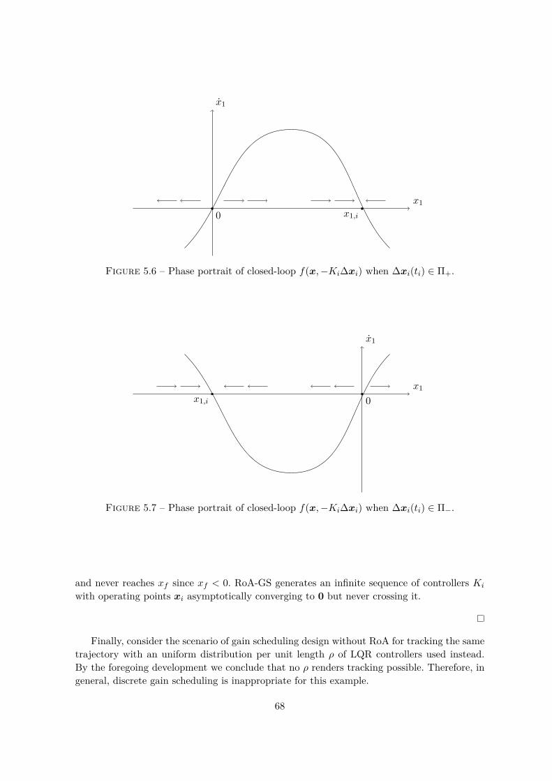
x1

x1

0 x1,i

Figure 5.6 – Phase portrait of closed-loop f(x,−Ki∆xi) when ∆xi(ti) ∈ Π+.

x1

x1

x1,i 0

Figure 5.7 – Phase portrait of closed-loop f(x,−Ki∆xi) when ∆xi(ti) ∈ Π−.

and never reaches xf since xf < 0. RoA-GS generates an infinite sequence of controllers Ki

with operating points xi asymptotically converging to 0 but never crossing it.

Finally, consider the scenario of gain scheduling design without RoA for tracking the sametrajectory with an uniform distribution per unit length ρ of LQR controllers used instead.By the foregoing development we conclude that no ρ renders tracking possible. Therefore, ingeneral, discrete gain scheduling is inappropriate for this example.

68

x1

x2

xf x0

R0

x1

R1

x2

R2Π

Figure 5.8 – Sequence of RoA-GS controllers Ki with associated Ri fails to cross the originand reach xf .

5.4 The quaternion uncontrollable linearized dynamics conun-drum

5.4.1 Quaternion attitude dynamics

Quaternion algebra formulation varies to a small extent in literature, but herein a quater-nion q ∈ (R4,×) is defined as

q =(q0q1

)(5.41)

where q0 ∈ R and q ∈ R3 equipped with quaternion product × operation defined as

p× q =(

p0q0 − p1 · q1p0q1 + q0p1 + p1 × q1

)(5.42)

The ill-posed property that the present section highlights when performing LQR controldesign in the quaternion formulation is present in both under and fully actuated systems.Therefore, for presentation clarity, we shall focus on the fully actuated version. Our proposedcontrol techniques are nonetheless seamlessly applicable to both cases. The fully actuatedattitude dynamics equations of motion in the quaternion formulation can be written as

q = 12

[0 −ωTω −[ω×]

](q0q1

)(5.43)

69

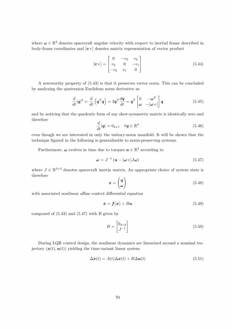
where ω ∈ R3 denotes spacecraft angular velocity with respect to inertial frame described inbody-frame coordinates and [v×] denotes matrix representation of vector product

[v×] =

0 −v3 v2v3 0 −v1−v2 v1 0

(5.44)

A noteworthy property of (5.43) is that it preserves vector norm. This can be concludedby analyzing the quaternion Euclidean norm derivative as

d

dt|q|2 = d

dt

(qTq

)= 2qT dq

dt= qT

[0 −ωTω −[ω×]

]q (5.45)

and by noticing that the quadratic form of any skew-symmetric matrix is identically zero andtherefore

d

dt|q| = 04×1 ∀q ∈ R4 (5.46)

even though we are interested in only the unitary-norm manifold. It will be shown that thetechnique figured in the following is generalizable to norm-preserving systems.

Furthermore, ω evolves in time due to torques u ∈ R3 according to

ω = J−1 (u− [ω×]Jω) (5.47)

where J ∈ R3×3 denotes spacecraft inertia matrix. An appropriate choice of system state istherefore

x =(q

ω

)(5.48)

with associated nonlinear affine control differential equation

x = f(x) +Bu (5.49)

composed of (5.43) and (5.47) with B given by

B =[04×3J−1

](5.50)

During LQR control design, the nonlinear dynamics are linearized around a nominal tra-jectory (x(t),u(t)) yielding the time-variant linear system

∆x(t) = A(t)∆x(t) +B∆u(t) (5.51)

70

For the quaternion attitude dynamics, straightforward differentiation yields

A(t) = ∂f

∂x=[∂q∂q

∂q∂ω

∂ω∂q

∂ω∂ω

]=

12

[0 −ωT (t)ω(t) −[ω(t)×]

]12

[−qT1 (t)

q0(t)I + [q1(t)×]

]03×4 [ω(t)×]− J−1[ω(t)×]J

(5.52)

Controllability and stabilizability of the system play a fundamental role in the design ofLQR controllers and, therefore, are studied in the following. Firstly, notice that (5.46) impliesthat the reachable set of the nonlinear system is included in

M = {q ∈ R4 : |q| = 1} $ R4 (5.53)

and therefore is not controllable. Additionally, the local linear model is not controllable either.This can be seen by a controllability normal form of the system which can be obtained bythe following change of coordinates

∆x′(t) = U(t)∆x(t) (5.54)

whereU(t) =

[Uq(t) 04×303×4 I3

](5.55)

andUq(t) =

[q0(t) qT1 (t)−q1(t) q0(t)I3 − [q1(t)×]

](5.56)

and therefore∆x′(t) = A′(t)∆x′(t) +B′(t)∆u(t) (5.57)

where 2

A′(t) = U(t)U−1(t)+U(t)A(t)U−1(t) =

12

[0 0T

0 −[ω(t)×]

]12

[0T

I3

]O3×3 [ω(t)×]− J−1[ω(t)×]J

(5.58)

andB′(t) = U(t)B =

[04×3J−1

](5.59)

Notice that (5.55) is a valid coordinate transformation since the matrix Uq representsa conjugate left product in quaternion space and, therefore, it is invertible for all non-zeroquaternions. From the linear system form in (5.58) and (5.59), we can conclude that the linearsystem is non-stabilizable (therefore uncontrollable) for all trajectories by looking at the firsttransformed state variable ∆x′1 dynamics, which is

∆x′1 = 0 ∀x(t),u(t) (5.60)

2. The algebra is tedious and therefore omitted. If an adventurous reader wishes to check the computations,the following identity is valuable : [y×]2 + ||y||2I = yyT .

71

Notice that the transformed system (A′, B′) is time-variant in general. However, if weconsider only reference trajectories that are constant in ω(t) = ω0 (hereafter denoted ω-trajectories), the system becomes time-invariant 3. Furthermore, the linear system has 6controllable modes for all ω-trajectories. This can be seen by means of the transformed system(A′, B′) Kalman controllability matrix K :

K =[B AB A2B · · ·

]=

0T 0T 0T · · ·03×3

12J−1 −1

2J−1[ω0×] · · ·

J−1 ∆J−1 ∆2J−1 · · ·

(5.61)

where∆ , [ω0×]− J−1[ω0×]J (5.62)

The lower triangular structure guarantees row rank 6 for all ω-trajectories. The control-lability properties exploited in this section are fundamental notions in the LQR design tofollow.

5.4.2 The time-invariant linear quadratic regulator

Consider the time-invariant linear system in state-space representation given by

x(t) = Ax(t) +Bu(t) (5.63)

where x(t) : R→ Rn, u(t) : R→ Rm, A ∈ Rn×n and B ∈ Rn×m are, respectively, state vector,input (or control) vector, system matrix and input matrix. We are interested in computingthe optimal control policy u∗(t) that minimizes the cost

J(x0,u) =ˆ ∞

0

(xTQx+ uTRu

)dt (5.64)

where x0 = x(0), Q ∈ Rn×n, R ∈ Rm×m are, respectively, initial state, positive semi-definitestate penalty and positive definite actuator penalty matrices. This strategy is called the linearquadratic regulator (LQR) [AM90]. By means of the Hamilton-Jacobi-Bellman equation, onecan show [AM90] that the control policy

u∗(t) = argminu

J(x0,u) (5.65)

for the system described by (5.63) is independent of x0 and is given by

u∗(t) = −R−1BTPx(t) (5.66)

3. Notice that our approach yields an alternative to Floquet’s theorem approach to computing U(t) for thepresent problem.

72

where P is the unique solution of the algebraic Riccati equation (ARE)

PA+ATP − PBR−1BTP +Q = 0 (5.67)

if (A,B) is stabilizable and (A,Q1/2) is detectable. The solution can be numerically computed[Lau78] ; [PCK91] and a figure of merit for its numerical stability, represented here by meansof its relative condition number, is [Bye85]

crel(A,B,Q,R) = 1||P ||F

(||Q||F ||Z1||2 + ||A||F ||Z2||2 + ||BR−1BT ||F ||Z3||2

)(5.68)

whereZ1 = T−1 (5.69)

Z2 = T−1(I ⊗ P + (P ⊗ I)Π

)(5.70)

Z3 = T−1(P ⊗ P ) (5.71)

andT = In ⊗ (A−BR−1BTP )T + (A−BR−1BTP )T ⊗ In (5.72)

with || · ||F , || · ||2 and ⊗ denoting, respectively, Frobenius norm, 2-norm and the Kroneckerproduct.

The LQR can be extended [AM90] to time-varying linear systems with an increase ofalgorithm complexity and required look-up table memory for implementation in robotics em-bedded systems. Fortunately, Sec. 5.4.1 proved that the attitude regulation and ω-trajectorytracking problems are time-invariant under appropriate change of coordinates. Be that as itmay, quaternion linearization was shown to suffer from lack of controllability in all operatingpoints precluding a theoretical LQR solution to exist or a numerically stable computationalsolution to be found. This shortcoming is addressed in the next sections.

5.4.3 The reduced quaternion model revisited

Intuitively, the lack of controllability in quaternion systems arrives from its non-minimalrepresentation that lives in a proper subset of R4. To address this issue, previous work [Yan16]rewrites (5.52) with, for instance, the first coordinate q0 of a quaternion in terms of the othercomponents such that

q0 = ±√

1− q21 − q2

2 − q23 (5.73)

and drops the redundant associate q0 lines and columns from the system. In a neighborhoodof an operating point in {(q,ω) : qTq = 1,ω ∈ R3} the signal ambiguity can be resolved. 4

Furthermore, previous work assumes a regulation problem, i.e., reference trajectory with

4. The careful reader will notice that a neighborhood of q0 = 0 might yield an ill-defined ambiguity.Nevertheless, one can argue that we should never choose such points as trimming points and proceed withcontroller design.

73

ω(t) = 0 for all t. These yield the so-called reduced quaternion model (Ar, Br) given by

Ar =[03×3

12

[±√

1− q21 − q2

2 − q23I + [q1×]

]03×3 03×3

](5.74)

andBr =

[03×3J−1

](5.75)

such that (∆q1∆ω

)= Ar

(∆q1∆ω

)+Br∆u (5.76)

Notice that the regulation problem assumption reduces the model to a linear time-invariantsystem whereas the deletion of redundant columns and lines potentially renders the systemcontrollable (and therefore eligible for LQR framework employment). Indeed, the controlla-bility matrix Kr of the reduced system yields

Kr =[Br ArBr A2

rBr · · ·]

=[03×3

12ΘJ−1 03×3 · · ·

J−1 03×3 03×3 · · ·

](5.77)

whereΘ , ±

√1− q2

1 − q22 − q2

3I + [q1×] (5.78)

Therefore, full row rank of Kr is conditioned to

det(1

2

(±√

1− q21 − q2

2 − q23I + [q1×]

)J−1

)= 1

8 detJ

∣∣∣∣∣∣∣q0 −q3 q2q3 q0 −q1−q2 q1 q0

∣∣∣∣∣∣∣ =±√

1− q21 − q2

2 − q23

8 detJ

(5.79)which allows one to conclude that the quaternion reduced model is globally controllable exceptfor q0 = 0 operating points. It is expected therefore a variable numerical stability in the spaceof configurations. Fig. 5.9 illustrates the condition number crel(Ar, Br, I, I) of the associatedRiccati problem in function of different ZYX -order Euler angles {ψ, θ, φ}, respectively, yaw,pitch and roll. We conclude that near-uncontrollable operating points are numerical unstabledelivering unreliable local optimal controllers.

Previous work [Yan16] regulates for q = (1, 0, 0, 0), and, therefore, does not encounterproblems. However, a wide attitude envelope quaternion operating point controller can runinto numerical problems calling for a more stable description. Furthermore, numerical stabilityover the whole configuration space is one of the most attractive properties of quaternions thatis undermined by the present LQR workflow.

We propose a solution to this problem by means of the transformation given in (5.54).

74

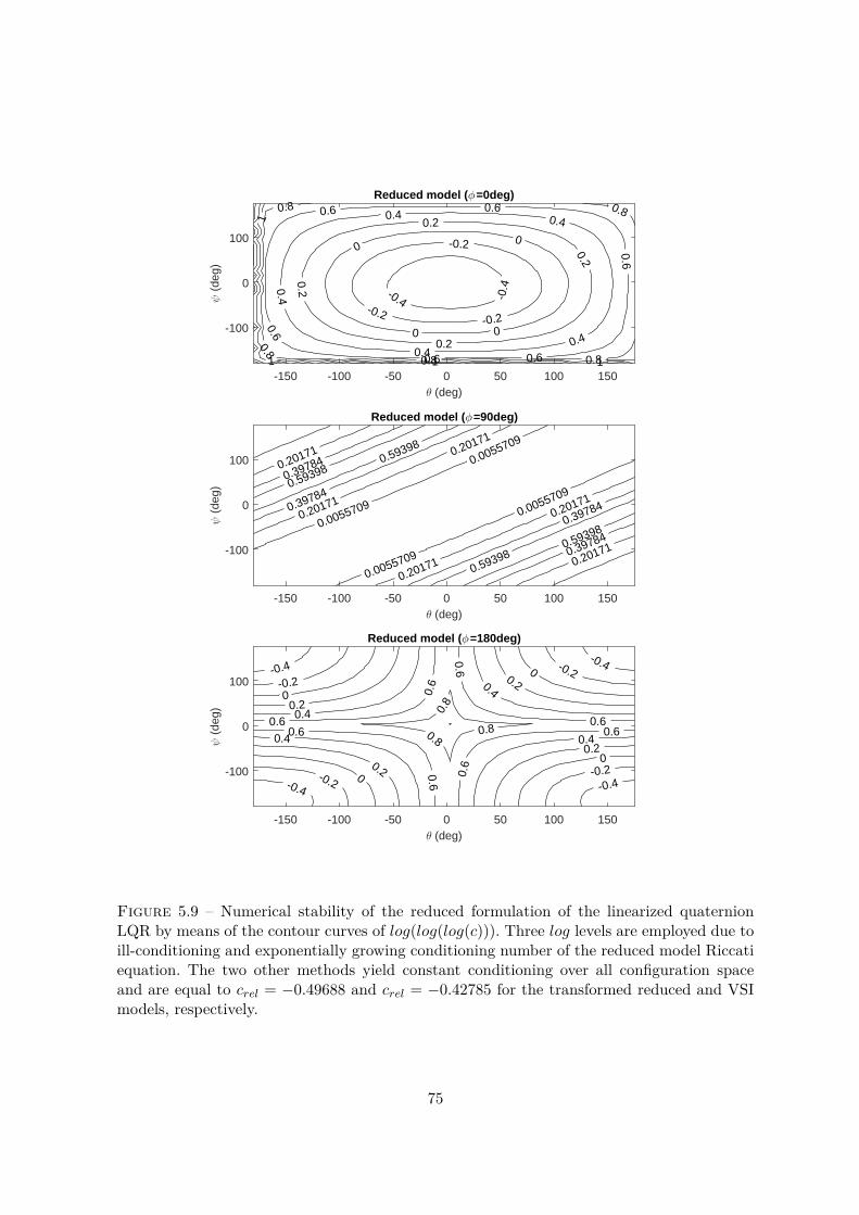
Reduced model (φ=0deg)

-0.4 -0.4

-0.2

-0.2

-0.20

00

00.2

0.2

0.2

0.2

0.4

0.4

0.4 0.4

0.4

0.6

0.6

0.6 0.6

0.6

0.6 0.80.8

0.8

0.8 0.8

111

1

-150 -100 -50 0 50 100 150θ (deg)

-100

0

100

ψ (

deg)

Reduced model (φ=90deg)

0.0055709

0.0055709

0.0055709

0.0055709 0.20171

0.20171

0.20171

0.20171

0.20171

0.20171

0.39784

0.39784

0.39784

0.39784

0.59398

0.59398

0.59398

0.59398

-150 -100 -50 0 50 100 150θ (deg)

-100

0

100

ψ (

deg)

Reduced model (φ=180deg)

-0.4-0.4

-0.4-0.4

-0.2-0.2

-0.2-0.2

0

0

0

0

0.20.2

0.2

0.2

0.40.4

0.4

0.4

0.6

0.60.6

0.6

0.6

0.6

0.6

0.60.8

0.8

0.8

-150 -100 -50 0 50 100 150θ (deg)

-100

0

100

ψ (

deg)

Figure 5.9 – Numerical stability of the reduced formulation of the linearized quaternionLQR by means of the contour curves of log(log(log(c))). Three log levels are employed due toill-conditioning and exponentially growing conditioning number of the reduced model Riccatiequation. The two other methods yield constant conditioning over all configuration spaceand are equal to crel = −0.49688 and crel = −0.42785 for the transformed reduced and VSImodels, respectively.

75

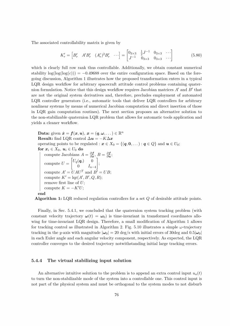
The associated controllability matrix is given by

K ′r =[B′r A′B′r (A′r)2B′r · · ·

]=[03×3

12J−1 03×3 · · ·

J−1 03×3 03×3 · · ·

](5.80)

which is clearly full row rank thus controllable. Additionally, we obtain constant numericalstability log(log(log(c))) = −0.49688 over the entire configuration space. Based on the fore-going discussion, Algorithm 1 illustrates how the proposed transformation enters in a typicalLQR design workflow for arbitrary spacecraft attitude control problems containing quater-nion formulation. Notice that this design workflow requires Jacobian matrices A′ and B′ thatare not the original system derivatives and, therefore, precludes employment of automatedLQR controller generators (i.e., automatic tools that deliver LQR controllers for arbitrarynonlinear systems by means of numerical Jacobian computation and direct insertion of thosein LQR gain computation routines). The next section proposes an alternative solution tothe non-stabilizable quaternion LQR problem that allows for automatic tools application andyields a cleaner workflow.

Data: given x = f(x,u), x = (q,ω, . . . ) ∈ RnResult: find LQR control ∆u = −K∆xoperating points to be regulated : x ∈ X0 = {(q,0, . . . ) : q ∈ Q} and u ∈ U0;for xi ∈ X0, ui ∈ U0 do

compute Jacobians A = ∂f∂x , B = ∂f

∂u ;

compute U =[Uq(qi) 0

0 In−4

];

compute A′ = UAUT and B′ = UB;compute K ′ = lqr(A′, B′, Q,R);remove first line of U ;compute K = −K ′U ;

endAlgorithm 1: LQR reduced regulation controllers for a set Q of desirable attitude points.

Finally, in Sec. 5.4.1, we concluded that the quaternion system tracking problem (withconstant velocity trajectory ω(t) = ω0) is time-invariant in transformed coordinates allo-wing for time-invariant LQR design. Therefore, a small modification of Algorithm 1 allowsfor tracking control as illustrated in Algorithm 2. Fig. 5.10 illustrates a simple ω-trajectorytracking in the y-axis with magnitude |ω0| = 20 deg/s with initial errors of 30deg and 0.5|ω0|in each Euler angle and each angular velocity component, respectively. As expected, the LQRcontroller converges to the desired trajectory notwithstanding initial large tracking errors.

5.4.4 The virtual stabilizing input solution

An alternative intuitive solution to the problem is to append an extra control input ua(t)to turn the non-stabilizable mode of the system into a controllable one. This control input isnot part of the physical system and must be orthogonal to the system modes to not disburb

76

Data: given x = f(x,u), x = (q,ω, . . . ) ∈ RnResult: find LQR control ∆u = −K∆xoperating points to be regulated : x ∈ X0 = {(q,0, . . . ) : q ∈ Q} and u ∈ U0;for xi ∈ X0, ui ∈ U0 do

compute Jacobians A = ∂f∂x , B = ∂f

∂u ;

compute U =[Uq(qi) 0

0 In−4

];

compute A′ = UAUT and B′ = UB;compute K ′ = lqr(A′, B′, Q,R);remove first line of U ;compute K = −K ′U ;

endAlgorithm 2: LQR reduced regulation controllers for a set Q of desirable attitude points.

real physical dynamics while affecting the zero dynamics found in (5.58). A natural directionis given, therefore, by the first line of the U(t) matrix given by (5.55) yielding the augmentedsystem (

q

ω

)= A

(q

ω

)+[B

q

0

](u

ua

)(5.81)

Notice that it matches our intuition in the sense that the virtual input should point inthe direction in which we have no control, which is the direction of the quaternion itself. Thereasoning behind this is illustrated by (5.45) and (5.46). Quaternions live in a 4-dimensionalsphere and its derivatives are restricted to the tangent of the sphere in a given point ofoperation q. Therefore, the direction q is, indeed, the most suitable direction for the artificialinput.

Additionally, we observe that instead of appending the virtual input at the linearizedmode, one can add it directly in the nonlinear model such that

x = f(x,u) +[q(t)0

]ua(t) (5.82)

since its linearization yields (with respect to operating point ua = 0)

∆x = ∂f

∂x∆x+ ∂f

∂u∆u+

[q(t)0

]ua(t) (5.83)

which results in a linearized artificial input in the desirable direction. The resulting linearizeddynamics are given by

Aa =

12

[0 −ωTω −[ω×]

]q 1

2

[−qT1

q0I + [q1×]

]03×4 0 [ω×]− J−1[ω×]J

(5.84)

77

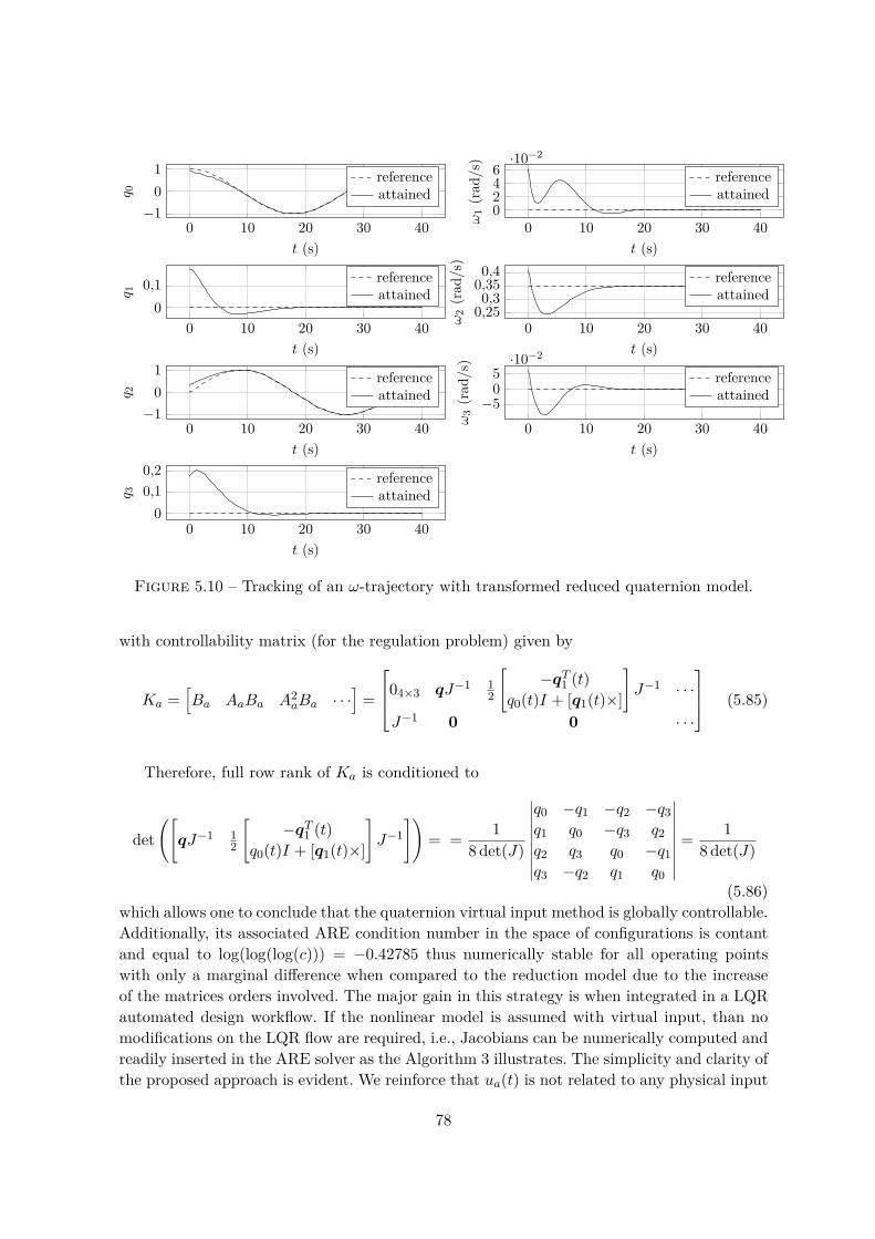
0 10 20 30 40−1

01

t (s)

q 0

referenceattained

0 10 20 30 400

0,1

t (s)

q 1

referenceattained

0 10 20 30 40−1

01

t (s)

q 2

referenceattained

0 10 20 30 400

0,10,2

t (s)

q 3

referenceattained

0 10 20 30 400246·10−2

t (s)

ω1(rad

/s)

referenceattained

0 10 20 30 400,250,3

0,350,4

t (s)

ω2(rad

/s)

referenceattained

0 10 20 30 40

−505·10−2

t (s)ω

3(rad

/s)

referenceattained

Figure 5.10 – Tracking of an ω-trajectory with transformed reduced quaternion model.

with controllability matrix (for the regulation problem) given by

Ka =[Ba AaBa A2

aBa · · ·]

=

04×3 qJ−1 12

[−qT1 (t)

q0(t)I + [q1(t)×]

]J−1 · · ·

J−1 0 0 · · ·

(5.85)

Therefore, full row rank of Ka is conditioned to

det([qJ−1 1

2

[−qT1 (t)

q0(t)I + [q1(t)×]

]J−1

])= = 1

8 det(J)

∣∣∣∣∣∣∣∣∣q0 −q1 −q2 −q3q1 q0 −q3 q2q2 q3 q0 −q1q3 −q2 q1 q0

∣∣∣∣∣∣∣∣∣ = 18 det(J)

(5.86)which allows one to conclude that the quaternion virtual input method is globally controllable.Additionally, its associated ARE condition number in the space of configurations is contantand equal to log(log(log(c))) = −0.42785 thus numerically stable for all operating pointswith only a marginal difference when compared to the reduction model due to the increaseof the matrices orders involved. The major gain in this strategy is when integrated in a LQRautomated design workflow. If the nonlinear model is assumed with virtual input, than nomodifications on the LQR flow are required, i.e., Jacobians can be numerically computed andreadily inserted in the ARE solver as the Algorithm 3 illustrates. The simplicity and clarity ofthe proposed approach is evident. We reinforce that ua(t) is not related to any physical input

78

in any sense and its corresponding component in the LQR gain K should be disregarded.

Data: given x = f(x,u) + (q,0, · · · )Tua, x = (q,ω, . . . ) ∈ RnResult: find LQR control ∆(u, ua)T = −K∆xoperating points to be regulated : x ∈ X0 = {(q,0, . . . ) : q ∈ Q} and u ∈ U0;for xi ∈ X0, ui ∈ U0 do

compute Jacobians A = ∂f∂x , B = ∂f

∂u ;compute K = lqr(A,B,Q,R);

endAlgorithm 3: LQR virtual regulation controllers for a set Q of desirable attitude points.

Finally, notice that the present technique is restricted to the regulation problem. Thetracking problem requires transformation of coordinates to be eligible to time-invariant LQRdesign.

5.4.5 The mixed parametrization solution

Finally, if one is not restricted to the use of quaternions in the entire design workflow, asimpler solution – from a theoretical point of view – is available to produce controllable locallinear approximations of quaternion dynamics. As previously done in Chap. 3, one can pursuea local Euler angle chart on top of the global quaternion description.

To conclude, we remark that, in view of the design workflow the control engineer pur-sues, either one of the aforementioned three solutions could be more appropriate in view oftheir particular features previously discussed. In our case study, we shall pursue the presentmixed parametrization solution since we defer polynomial optimization trajectory planningtechniques to future work.

5.5 The MAVion control architecture

This section exploits the nonlinear global model derived in Sec. 3.1 to provide a velocitycontroller for the MAVion in view of the piloting interface defined in Sec. 3.4. Recall that weobtained a mathematical description of the form x = f(x,u), where

x =(vb ωb q

)(5.87)

andu =

(ω1 ω2 δ1 δ2

)(5.88)

Furthermore, we obtained local linear models for all operating points in Chap. 3 of the form

d

dt∆x = A∆x+B∆u (5.89)

79

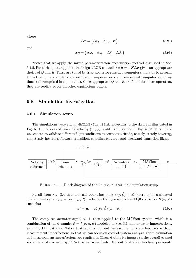
where∆x =

(∆vb ∆ωb ψ

)(5.90)

and∆u =

(∆ω1 ∆ω2 ∆δ1 ∆δ2

)(5.91)

Notice that we apply the mixed parametrization linearization method discussed in Sec.5.4.5. For each operating point, we design a LQR controller ∆u = −K∆x given an appropriatechoice of Q and R. These are tuned by trial-and-error runs in a computer simulator to accountfor actuator bandwidth, state estimation imperfections and embedded computer samplingtimes (all comprised in simulation). Once appropriate Q and R are found for hover operation,they are replicated for all other equilibrium points.

5.6 Simulation investigation

5.6.1 Simulation setup

The simulations were run in MATLAB/Simulink according to the diagram illustrated inFig. 5.11. The desired tracking velocity (vf , ψ) profile is illustrated in Fig. 5.12. This profilewas chosen to validate different flight conditions at constant altitude, namely, steady hovering,non-steady hovering, forward transition, coordinated curve and backward transition flight.

Velocityreference

Gainscheduler

LQR Actuatorsmodel

MAVionx = f(x,u)

vf , ψ xr +−

∆x

K,xr,ur

u∗ u x

Figure 5.11 – Block diagram of the MATLAB/Simulink simulation setup.

Recall from Sec. 3.4 that for each operating point (vf , ψ) ∈ R2 there is an associateddesired limit cycle xref = (vb,ωb, q(t)) to be tracked by a respective LQR controller K(vf , ψ)such that

u∗ = ur −K(vf , ψ) (x− xr) (5.92)

The computed actuator signal u∗ is then applied to the MAVion system, which is acombination of the dynamics x = f(x,u,w) modeled in Sec. 3.1 and actuator imperfections,as Fig. 5.11 illustrates. Notice that, at this moment, we assume full state feedback withoutmeasurement imperfections so that we can focus on control system analysis. State estimationand measurement imperfections are studied in Chap. 6 while its impact on the overall controlsystem is analyzed in Chap. 7. Notice that scheduled-LQR control strategy has been previously

80

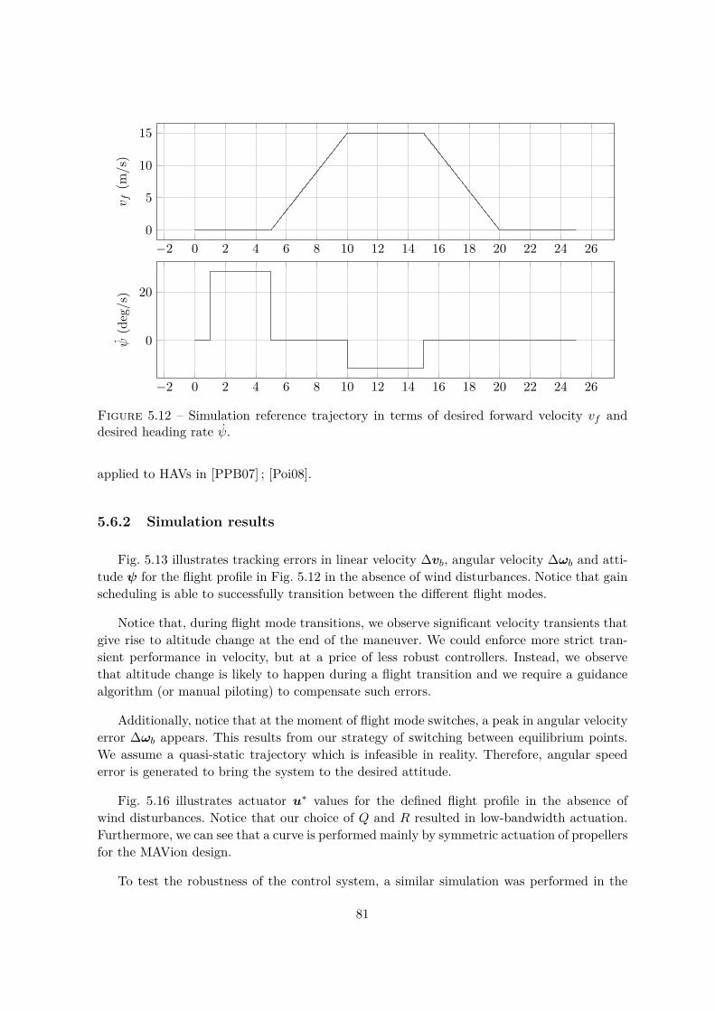
−2 0 2 4 6 8 10 12 14 16 18 20 22 24 260

5

10

15v f

(m/s)

−2 0 2 4 6 8 10 12 14 16 18 20 22 24 26

0

20

ψ(deg/s)

Figure 5.12 – Simulation reference trajectory in terms of desired forward velocity vf anddesired heading rate ψ.

applied to HAVs in [PPB07] ; [Poi08].

5.6.2 Simulation results

Fig. 5.13 illustrates tracking errors in linear velocity ∆vb, angular velocity ∆ωb and atti-tude ψ for the flight profile in Fig. 5.12 in the absence of wind disturbances. Notice that gainscheduling is able to successfully transition between the different flight modes.

Notice that, during flight mode transitions, we observe significant velocity transients thatgive rise to altitude change at the end of the maneuver. We could enforce more strict tran-sient performance in velocity, but at a price of less robust controllers. Instead, we observethat altitude change is likely to happen during a flight transition and we require a guidancealgorithm (or manual piloting) to compensate such errors.

Additionally, notice that at the moment of flight mode switches, a peak in angular velocityerror ∆ωb appears. This results from our strategy of switching between equilibrium points.We assume a quasi-static trajectory which is infeasible in reality. Therefore, angular speederror is generated to bring the system to the desired attitude.

Fig. 5.16 illustrates actuator u∗ values for the defined flight profile in the absence ofwind disturbances. Notice that our choice of Q and R resulted in low-bandwidth actuation.Furthermore, we can see that a curve is performed mainly by symmetric actuation of propellersfor the MAVion design.

To test the robustness of the control system, a similar simulation was performed in the

81

−2 0 2 4 6 8 10 12 14 16 18 20 22 24 26

−2

0

2

4∆vb(m

/s)

vb1vb2vb3

−2 0 2 4 6 8 10 12 14 16 18 20 22 24 26−50

0

50

∆ωb(deg/s)

ωb1ωb2ωb3

−2 0 2 4 6 8 10 12 14 16 18 20 22 24 26−20

−10

0

10

20

t (s)

ψ(deg)

ψ1ψ2ψ3

Figure 5.13 – Tracking errors in linear velocity ∆vb, angular velocity ∆ωb and attitude ψfor the defined flight profile without wind disturbances.

presence of an alternating wind disturbance wl in local NED coordinates such that (in m/s)

wl = 2 sin(π

2 t)(

1 1 0)T

(5.93)

Its associated tracking errors and actuator inputs are illustrated in Figs. 5.15 and 5.16.Notice that all maneuvers are successfully performed in spite of the disturbances.

5.7 Closing remarks

In this chapter we discuss control design issues specific to tail-sitters and highly maneuve-rable vehicles. Furthermore, we lay the necessary theoretical and technical foundations for SOSpolynomial optimization motion planning. To this end, we revisit the problem of employingLQR design in quaternion-based linearized systems for local control of complex underactua-

82

−2 0 2 4 6 8 10 12 14 16 18 20 22 24 26300

400

500

Prop

ellerspeed(rad

/s)

ω1ω2

−2 0 2 4 6 8 10 12 14 16 18 20 22 24 26−30

−20

−10

0

t (s)

Elevon

defle

ction(deg)

δ1δ2

Figure 5.14 – Actuator u values for the defined flight profile without wind disturbances.

ted systems. We warn of numerically unstable regions in a popular algorithm and proposethree alternative solutions that yield constant low relative condition numbers for the entireconfiguration space. Two of them are novel contributions. The first solution is built on topof the commonplace solution whereas the second one is an elegant and simple reformulationsuited for applications that require minimal intrusion in the classical LQR design workflow.We also demonstrate how to adapt the first solution to the constant angular velocity trackingproblem. Finally, a gain-scheduled LQR controller is designed for the MAVion and validatedby simulation in view of MAVion embedded system sampling time and actuators bandwidth.

Additionally, we prove by means of an analytical counterexample that global controllabi-lity does not imply successful RoA-GS nor gain scheduling quasi-static trajectory tracking.Fortunately, this is not the case with the MAVion. Future work might include sufficient condi-tions for RoA-GS trajectory tracking.

83

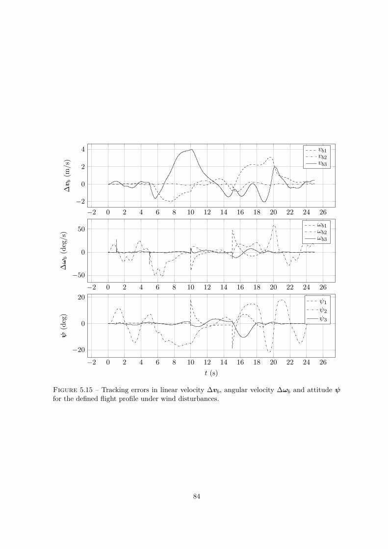
−2 0 2 4 6 8 10 12 14 16 18 20 22 24 26−2

0

2

4

∆vb(m

/s)

vb1vb2vb3

−2 0 2 4 6 8 10 12 14 16 18 20 22 24 26−50

0

50

∆ωb(deg/s)

ωb1ωb2ωb3

−2 0 2 4 6 8 10 12 14 16 18 20 22 24 26

−20

0

20

t (s)

ψ(deg)

ψ1ψ2ψ3

Figure 5.15 – Tracking errors in linear velocity ∆vb, angular velocity ∆ωb and attitude ψfor the defined flight profile under wind disturbances.

84

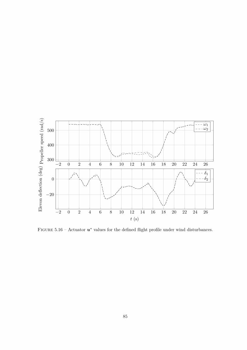
−2 0 2 4 6 8 10 12 14 16 18 20 22 24 26300

400

500

Prop

ellerspeed(rad

/s)

ω1ω2

−2 0 2 4 6 8 10 12 14 16 18 20 22 24 26

−20

0

t (s)

Elevon

defle

ction(deg)

δ1δ2

Figure 5.16 – Actuator u∗ values for the defined flight profile under wind disturbances.

85

Chapitre 6

Navigation system design

Sommaire6.1 Introduction . . . . . . . . . . . . . . . . . . . . . . . . . . . . . . . . . . 87

6.1.1 Contextualization . . . . . . . . . . . . . . . . . . . . . . . . . . . . . . . 876.1.2 Reference frames definition . . . . . . . . . . . . . . . . . . . . . . . . . . 89

6.2 Avionics modeling . . . . . . . . . . . . . . . . . . . . . . . . . . . . . . . 896.3 Complementary filtering revisited . . . . . . . . . . . . . . . . . . . . . 91

6.3.1 Filter description . . . . . . . . . . . . . . . . . . . . . . . . . . . . . . . . 916.3.2 Complementary filter misalignment linearized error model . . . . . . . . . 936.3.3 Convergence local analysis . . . . . . . . . . . . . . . . . . . . . . . . . . . 95

6.4 The CF-EKF filter . . . . . . . . . . . . . . . . . . . . . . . . . . . . . . . 966.5 Simulation investigation . . . . . . . . . . . . . . . . . . . . . . . . . . . 97

6.5.1 Simulation setup . . . . . . . . . . . . . . . . . . . . . . . . . . . . . . . . 976.5.2 Simulation results . . . . . . . . . . . . . . . . . . . . . . . . . . . . . . . 98

6.6 Final remarks . . . . . . . . . . . . . . . . . . . . . . . . . . . . . . . . . . 98

6.1 Introduction

6.1.1 Contextualization

Although more often than not overlooked, state estimation systems play a fundamentalrole in applied control systems theory. Careless observer design, for instance, gives rise to –often avoidable – overall autopilot performance loss. Moreover, navigation 1 systems in microair vehicles (MAVs) call for low-cost sensors and pose a challenge for the observer designer.More specifically, it is well known that stand-alone inertial navigation systems (INS) havetheir errors diverging with time. Consequently, an upper bound on the duration of stand-aloneINS systems precludes their use in low-cost MAVs. The traditional approach for solving suchinconvenience is to resort to aiding devices such as global navigation satellite system (GNSS)receivers, magnetometers and/or sighting devices. Two philosophies have been extensively

1. While in the Robotics domain the task of calculating one’s current position and velocity is designated aslocalization, we shall use in this thesis the commonplace navigation denomination ubiquitously present acrossthe Aerospace Engineering literature.

87

applied to perform this data fusion : extended Kalman filtering (EKF) and complementaryfiltering (CF).

Some key similarities and differences between EKF and CF are discussed in [Hig75]. Forinstance, a CF is equivalent to an EKF under steady-state conditions. However, navigationerrors dynamics and observability are dependent on vehicle trajectory [GMBI90] ; [GMBI92]in such a way that an EKF can outperform a CF in manoeuvring conditions. Be that as it may,the use of low-cost sensors renders the EKF suboptimal and often inconsistent due to largenavigation error covariances that undermine linearization assumptions. Particle filters [GSS93]have been employed to solve such problem but require a fair amount of computational poweroften not available in low-cost or MAV applications. CF, on the other hand, is an exceptionallyinexpensive filter.

Previous work [Eus+08] has shown that the CF can be robustly applied to low-cost sensorsand achieve performance that is comparable to that of a full suboptimal EKF based onGNSS-aided inertial measurement unit (IMU/GNSS) when vehicle dynamics is taken intoconsideration by means of airspeed measurements. Another strategy to relax the CF requiredassumption of constant velocity motion is to apply gains that adapt to the motion to beestimated [CYB11]. The issue of tuning a given CF is discussed in detail in [Vas+09] to shapea frequency response that blends the frequency contents of the aiding devices and the inertialsensors (implementation aspects are also highlighted). [MHP05] compares two implementationarchitectures for the CF, namely, direct CF and passive CF, and shows that the latter hassuperior dynamical properties, proves its convergence and extends it to provide adaptiverate-gyro drift estimation. Similarly, [PHS07] provides a nonlinear attitude and rate-gyrodrift estimator for an UAV.

The present case study exploits the passive CF for position, velocity and attitude esti-mation employing a magnetometer as an external aid to bound attitude errors. On top ofthat, an external EKF is applied to restrain position and velocity errors by means of GNSSmeasurements. To the authors’ knowledge, there is no previous work on how to seamlesslyconnect both filters, although there are ad-hoc CF-EKF filter connection and tuning [JT07].This thesis contributes by delineating the overall CF-EKF filter structure designed to simplifythe tedious tuning process, studying some of its properties and delivering implementation de-tails. Furthermore, some EKF aiding devices (sighting devices, for instance) call for operatingsystems that increase system complexity thus reducing INS reliability. In view of this, I showhow to effectively employ CF-EKF in a multi-platform embedded system to implement faultisolation by running the CF stage in a separate low-throughput low-level reliable machine forstand-alone degraded mode operation.

In the following, an attitude passive CF based on gravitational and magnetic fields isreviewed (Sec. 6.3.1) and its dynamic properties are discussed (Sec. 6.3.3). Moreover, thiswork contributes by delivering an error model of this complementary filter based on psi-angle[WBI78] representation (Sec. 6.3.2) for statistical error analysis and extended Kalman orinformation filter integration (Sec. 6.4). The proposed framework is evaluated by means of adistributed loosely-coupled IMU/GNSS Kalman filter applied to synthetic IMU/GNSS sensordata (Sec. 6.5). Finally, concluding remarks and perspectives are presented (Sec. 6.6).

88

6.1.2 Reference frames definition

The low-cost strapdown inertial navigation nature of the proposed estimator motivates thedefinition of three reference frames as illustrated in Fig. 6.1. The inertial frame I is assumedstationary with respect to Earth since this thesis targets low-cost sensors that possess lowrate-gyro precision in view of Earth angular velocity. On the other hand, the body frame B

is fixed in the inertial measurement unit (IMU) and provides a natural vector space basisfor sensor measurements. Finally, an embedded processor collects sensors data and computesIMU position and attitude with respect to I by means of a complementary filter (see Sec. 6.3).Due to INS imperfections (e.g., sensors biases, noise, finite sampling frequency) the estimatedorientation of B is misaligned and it is defined as computed frame C.

B

C

ψ

δp

I

pb

pc

Figure 6.1 – Reference frames illustration. The inertial (I), body (B) and computed (C)frames are fixed, respectively, to Earth, IMU and estimated orientation by the attitude com-plementary filter.

6.2 Avionics modeling

Table 6.1 summarizes the available on-board avionics (and their precision) for navigationpurposes. Inertial sensors specifications are readily determined from manufacturer datasheet.On the other hand, the GNSS receiver manufacturer datasheet lacks noise and bias statistics(understandably, since GNSS receiver loosely-coupled position and velocity errors are hardlyGaussian). Therefore, I recast the available information as somewhat equivalent Gaussiannoise and bias quantities (in view of suboptimal Kalman filtering implementation).

Remark 6.1For indoor flight GNSS receiver position and velocity measurements are replaced by themotion capture system estimates described in Sec. 4.3. Since my focus is on outdoor flight,

89

Function Device Noise (typ) Bias (typ)Rate-gyro MPU-9150 0.005 (o/s/

√Hz) 20 (o/s)

Accelerom. MPU-9150 400 (µg/√Hz) 150 (mg)

Magnetom. MPU-9150 N/A N/AGNSS pos. NEO-6M σ = 2.5 (m) 0 (m)GNSS vel. NEO-6M σ = 0.1 (m/s) 0 (m/s)

Table 6.1 – Avionics subset for loosely-coupled GNSS and magnetometer aided strapdowninertial navigation.

the navigation system purposefully discards the high precision attitude measurements fromthe motion capture system. The ground control station, on the other hand, logs this data forattitude ground truth purposes.

For simulation and observer design, rate-gyro measurements ω(t) ∈ R3 are modeled as asuperposition of the nominal value iωbb(t), a random constant (with respect to B) Gaussiandrift εb ∼ N(0,Σε) and white Gaussian noise νgb (t) ∼ N(0,Σg) such that

ω(t) = iωbb(t) + εb + νgb (t) (6.1)

Similarly, accelerometer, magnetometer and GNSS receiver position and velocity measu-rements, respectively, f(t) ∈ R3, b(t) ∈ R3, λ(t) ∈ R3 and Υ(t) ∈ R3 are modeled as

f(t) = iabb(t)− gb(t) + ∇b + νab (t) (6.2)

b(t) = Bb(t) + ∆b + νmb (t) (6.3)

λ(t) =(λ(t) Λ(t) h(t)

)T+ νs(t) (6.4)

andΥ(t) = ivbl (t) + νvl (t) (6.5)

where ∇b ∼ N(0,Σ∇), νab (t) ∼ N(0,Σa), ∆b ∼ N(0,Σ∆), νmb (t) ∼ N(0,Σm), and g denote,respectively, accelerometer/magnetometer bias/noise, and Earth gravitational acceleration(indistinguishable from gravity in view of the stationary Earth assumption). Additionally,λ, Λ and h denote, respectively, vehicle latitude, longitude and altitude (LLA) in WGS84coordinates.

Notice that ∆b, although time-independent, accounts for drone hard iron biases and elec-tromagnetic interferences (EMI). In MAVs, the latter is mostly due to on-board electric mo-tors. Nevertheless, assuming estimation and control routines have a backend bilateral com-munication channel, motor speed is known and magnetic field a priori compensation in ∆b

can be pursued. Fig. 6.2 illustrates EMI impact on a stationary MAVion embedded magneto-meters due to symmetric (i.e., same rotation speed ω1 = ω2) motors actuation. Notice that,without bias compensation, high motor speeds triple the attitude error.

90

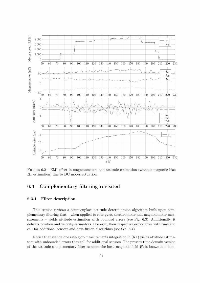
50 60 70 80 90 100 110 120 130 140 150 160 170 180 190 200 210 220 2300

2 0004 0006 0008 000

Motor

speed(R

PM)

|ω1||ω2|

50 60 70 80 90 100 110 120 130 140 150 160 170 180 190 200 210 220 230−50

0

50

Mag

netometer

(µT)

bb1bb2bb3

50 60 70 80 90 100 110 120 130 140 150 160 170 180 190 200 210 220 230

−1

0

1

Rate-gy

ro(deg/s)

ωb1ωb2ωb3

50 60 70 80 90 100 110 120 130 140 150 160 170 180 190 200 210 220 230

5

10

15

t (s)

Attitu

deerror(deg)

ψ

Figure 6.2 – EMI effect in magnetometers and attitude estimation (without magnetic bias∆b estimation) due to DC motor actuation.

6.3 Complementary filtering revisited

6.3.1 Filter description

This section reviews a commonplace attitude determination algorithm built upon com-plementary filtering that – when applied to rate-gyro, accelerometer and magnetometer mea-surements – yields attitude estimation with bounded errors (see Fig. 6.3). Additionally, itdelivers position and velocity estimators. However, their respective errors grow with time andcall for additional sensors and data fusion algorithms (see Sec. 6.4).

Notice that standalone rate-gyro measurements integration in (6.1) yields attitude estima-tors with unbounded errors that call for additional sensors. The present time-domain versionof the attitude complementary filter assumes the local magnetic field Bi is known and com-

91

ComplementaryFilter

ω(t)f(t)b(t)

qic(t)pci (t)ivci (t)

Figure 6.3 – Input-output schematic view of the quaternion complementary filter.

pares a predicted measurement Bc with an ideal measurement Bb to produce a residual thatis closely related to attitude errors, as we shall show in the following. Mathematically, noticethat

Bb ×Bc = −[Bc×]Bb = −[Bc×]DcbBc (6.6)

where Dcb is the DCM that transforms computed frame coordinates into body axes compo-

nents. Assuming a 3− 2− 1 rotation order of ψ3, ψ2 and ψ1, respectively, Dcb can be written

as

Dcb =

cψ2cψ3 cψ2sψ3 −sψ2sψ1sψ2cψ3 − cψ1sψ3 cψ1cψ3 + sψ1sψ2sψ3 sψ1cψ2sψ1sψ3 + cψ1sψ2cψ3 cψ1sψ2sψ3 − sψ1cψ3 cψ1cψ2

(6.7)

If small error angles ψi are assumed, cosψi → 1, sinψi → ψi, and (6.7) is simplified toread as

Dcb =

1 ψ3 −ψ2−ψ3 1 ψ1ψ2 −ψ1 1

= I − [ψ×] (6.8)

whereψ =

(ψ1 ψ2 ψ3

)T(6.9)

Therefore, (6.6) can be simplified to read

Bb ×Bc = −[Bc×](I − [ψ×])Bc = −[Bc×]2ψ (6.10)

Assuming the local gravitational vector is known, a similar development yields

gb × gc = −[gc×]2ψ (6.11)

Eqs. (6.10) and (6.11) contain candidates for feedback stabilization of ψ as a consequenceof their proportionality to ψ. Accordingly, an estimator iωcc for iωbb, namely, the angularvelocity of the body reference frame B with respect to the inertial frame I described in thebody axes B, is defined as

iωcc = ω − kaf × gc + kmb×Bc (6.12)

where ka, km > 0. Notice that the accelerometer term in (6.12) flips sign due to its negativemeasurement of gravity (i.e., −gb). From the embedded processor point of view, (6.12) can

92

be computed asiωcc = ω − kaf ×Di

cgi + kmb×DicBi (6.13)

where Dic is computed by means of qic, which can be computed by numerically integrating the

following classic [SL03] quaternion differential equation

d

dtqic = 1

2

[0 −(iωcc)Tiωcc −[iωcc×]

]qic (6.14)

and quaternion to DCM transformation equation

Dic =

(1− 2q22 − 2q2

3) 2(q1q2 + q0q3) 2(q1q3 − q0q2)2(q1q2 − q0q3) (1− 2q2

1 − 2q23) 2(q2q3 + q0q1)

2(q1q3 + q0q2) 2(q2q3 − q0q1) (1− 2q21 − 2q2

2)

(6.15)

Furthermore, gi = (0, 0, g), and Bi is location dependent 2 and assumed known. Bi canbe previously measured or computed, for instance, by means of the World Magnetic Model(WMM) [Chu+15] or the International Geomagnetic Reference Field (IGRF) [Fin+10].

Finally, position and velocity estimators are obtained by means of direct integration ofthe following mechanization equations

d

dtpci = ivci (6.16)

andd

dtivci = Dc

if + gi (6.17)

Taken together, (6.13), (6.14), (6.15), (6.16) and (6.17) implement the CF inertial navi-gation algorithm of Fig. 6.3. In the next two sections, some of its properties are re-derivedin view of the misalignment model, which is the main contribution of this chapter and thenecessary foundation for CF-EKF interfacing.

6.3.2 Complementary filter misalignment linearized error model

This section develops an error model for ψ(t), i.e., a stochastic differential equation thatmodels complementary filter inertial navigation errors in time due to vehicle motion anduncertainties in sensors.

Initially, notice that ψ(t) is composed by Euler angles and their relation to angular velocity

2. In a time scale substantially longer than typical aerial vehicle endurance values, Bi is also time-dependent.

93

is dictated by [SL03]

d

dtψ =

1 tanψ2 sinψ1 tanψ2 cosψ10 cosψ1 − sinψ10 sinψ1

cosψ2cosψ1cosψ2

cωbb (6.18)

Assuming small ψ and gathering only first order terms, we can write

d

dtψ = cωbb (6.19)

so thatd

dtψ = iωbb − iωcb = iωbb −Dc

b · iωcc = iωbb − iωcc + [ψ×]iωcc (6.20)

by means of (6.8). Therefore,

iωbb − iωcc = d

dtψ + [iωcc×]ψ (6.21)

Substituting (6.1), (6.2), (6.12) into (6.21), we obtain

dψ

dt=(− [iωcc×] + km[Bc×]2 + ka[gc×]2

)ψ+

(− I

)εb +

(− ka[gc×]

)∇b +

(km[Bc×]

)∆b+

+(− I

)νgb +

(km[Bc×]

)νmb +

(− ka[gc×]

)νab +

(− ka[gc×]

)iabb (6.22)

On the other hand, the errors on position and velocity, namely,

δp , pc − pb (6.23)

andδv , ivc − ivb (6.24)

have the following well-known differential equations for their time evolution [BSLK01]

d

dtδpi = δvi (6.25)

andd

dtδvi = Dc

i [f×]ψ +Dci∇b +Dc

iνab (6.26)

Eqs. (6.22), (6.25) and (6.26) describe errors stochastic time evolution in the CF inertialnavigation algorithm and can be used for several purposes, e.g., algorithm stability analysis(Sec. 6.3.3) and Kalman filtering data fusion (Sec. 6.4).

94

6.3.3 Convergence local analysis

Given sensors noise and bias characteristics, (6.22) provides the means to statisticallypredict the performance of the CF (for small ψ). Furthermore, it describes the dynamics ofthe attitude estimation error ψ(t). Considering bias and noise quantities as filter inputs, thelocal stability of the attitude CF is determined by the following linear time-variant system

dψ

dt=(− [iωcc×] + km[Bc×]2 + ka[gc×]2

)︸ ︷︷ ︸

N

ψ (6.27)

Although ψ has no physical meaningful basis (among other, rotations do not have a vectorspace structure), one can assign a basis to ψ and treat it as if it was a vector algebraically.Since (6.27) is fully described in computed basis, we assign the C basis to ψ such that

dψcdt

+ [iωcc×]ψc =(km[Bc×]2 + ka[gc×]2

)ψc (6.28)

The reasoning that transformed (6.27) into (6.28) is subtle but allows one to evoke thetransport theorem from classical mechanics and rewrite the left-hand side as(dψi

dt

)c

=(km[Bc×]2 + ka[gc×]2

)ψc (6.29)

such thatdψidt

= Dci

(km[Bc×]2 + ka[gc×]2

)︸ ︷︷ ︸

M

Dicψi (6.30)

The interested reader can quickly check that every matrix of the form [v×]2 has eigenvaluesλ1 = 0, with algebraic multiplicity 1, and λ2 = −|v|2 with algebraic multiplicity 2. Therefore,M is a linear combination of such matrices and it is negative semi-definite if km > 0 andka > 0. Therefore, the CF filter is marginally stable 3 for attitude determination.

Position and velocity estimation errors, on the other hand, remains unbounded and callfor additional sensors, which are commonly integrated by means of Kalman filters. Section6.4 provides a clean strategy to easily integrate and tune an EKF on top of a complementaryfilter.

3. More precisely, it is stable except for the unlikely case when B is parallel to g.

95

6.4 The CF-EKF filter

In the light of the foregoing development, it is convenient to define the EKF state vectoras

x =(δpi δvi ψ ∇b εb ∆b

)T(6.31)

and process noise asw =

(νab νgb νmb

iabb

)T(6.32)

such thatx = Ax+Bw (6.33)

where A and B can be obtained by inspection of (6.22), (6.25) and (6.26), yielding

A =

0 I 0 0 0 00 0 Dc

i [f×] Dci 0 0

0 0 N −ka[gc×] −I km[Bc×]0 0 0 0 0 00 0 0 0 0 00 0 0 0 0 0

(6.34)

and

B =

0 0 0 0Dci 0 0 0

−ka[gc×] −I km[Bc×] −ka[gc×]0 0 0 00 0 0 00 0 0 0

(6.35)

On the other hand, the EKF observation equation is dependent on the available aidingsensors. In this case study, a loosely-coupled GNSS receiver architecture [FB98] is employedsuch that

y = Hx+ v (6.36)

whereH =

[I3×3 03×3 03×1203×3 I3×3 03×12

](6.37)

and v is dependent on GNSS receiver uncertainties. After discretization of (6.33), the EKF isapplied (for a comprehensive discussion on Kalman filtering and useful equivalent alternativeformulations for use in low-cost architectures, see [May79]) and estimation of navigationerrors and sensor biases is performed. After each EKF update step, the state x is used forCF correction (position, velocity and attitude feedback) and sensor on-line calibration. Fig.6.4 illustrates the overall architecture.

A remarkable feature of the CF-EKF is that given the statistics of the noise processdefined by (6.32), one can straightforwardly tune the EKF stage by means of manufacturer

96

ComplementaryFilter

ω(t)

f(t)

b(t)

qic(t)

pci (t)

ivci (t)ExtendedKalmanFilter

BasicSensors

δp(t), δv(t), ψ(t) (correction)

AidingSensors

∇(t), ε(t), ∆(t) (calibration)

Figure 6.4 – CF-EKF filter overall architecture.

sensor specs and IMU sampling rate. However, the last noise component, namely, iabb, is rarelywhite nor Gaussian in reality. Therefore, it is the only noise component that might requiretrial-and-error tuning and careful consideration of vehicle dynamics.

6.5 Simulation investigation

6.5.1 Simulation setup

Two scenarios were simulated to assess CF-EKF performance in view of the availableavionics : (i) standalone attitude CF with raw GNSS receiver velocity measurements (see Fig.6.5) and (ii) CF-EKF fusion solution (see Fig. 6.6). Notice that the employed vehicle testtrajectory is the same as obtained in Sec. 5.6, which desired reference was given in Fig. 5.12and repeated here in Fig. 6.7 for the sake of completeness. However, the estimated state is notemployed for LQR feedback control. Instead, the real state x is used. In this way, we focuson navigation performance isolated from controller dynamics. The full system is simulated inthe next chapter.

Our objective in this experiment is to assess how CF-EKF performance compares to thatof a standalone CF with raw GNSS receiver velocity measurements. Notice that we studya very particular situation and further experiments are necessary to evaluate the generalemploybility of the CF-EKF filter, and is is out of the scope of this thesis. Our sole purposeis to analyze whether a Kalman filter is advantageous or not in our design (assuming onlyCF-filtered measurements are available by our autopilot firmware).

Finally, in view of the low quality of the employed sensors, biases are hardly constant and

97

Velocityreference

Gainscheduler

LQR Actuatorsmodel

MAVionx = f(x,u)

vf , ψ xr +−

∆x

K,xr,ur

u∗ u x

Magnetometer

IMU

GNSS receiver

ComplementaryFilter

Demux

qv

ψ

δv

+-

+-

Figure 6.5 – Block diagram of the MATLAB/Simulink simulation setup for the CF standa-lone experiment.

we decided to set biases to zero while increasing their noise values to compensate for floatingbiases values. Therefore, we do not attempt to estimate biases in this example, although ouroriginal filter structure allows one to do so.

6.5.2 Simulation results

Fig. 6.8 illustrates navigation errors in velocity δvi and attitude ψ while performing thedesignated flight profile for both implementations.

At a first glance, the CF and CF-EKF filters have similar performance. In this particularcase, the CF outperforms the CF-EKF during hover flight, while in other modes our expe-riment is inconclusive. Furthermore, in presence of noisy sensors, we observe a noisy outputfor the CF-EKF. Those remarks lead us to design the embedded MAVion navigation systemwith the standalone CF algorithm. We’ve concluded that the EKF would increase systemcomplexity with no visible gain in performance. Of course, further studies must be conduc-ted to assess which situations would benefit from our CF-EKF. A possibility would be in ascenario with sensors with systematic biases (that is, with modelable bias dynamics).

6.6 Final remarks

This chapter laid the foundation for CF and EKF interfacing without imposing excessivesuboptimal assumptions that often reduce performance and make it impracticable for tuning.While CF employed IMU/magnetometer measurements to bound attitude errors, an externalEKF bounded position and velocity errors by means of CF output and GNSS measurements.

98

Velocityreference

Gainscheduler

LQR Actuatorsmodel

MAVionx = f(x,u)

vf , ψ xr +−

∆x

K,xr,ur

u∗ u x

Magnetometer

IMU

GNSS receiver

CF

Demux

qv

ψ

δv

+-

+-

EKF

Figure 6.6 – Block diagram of the MATLAB/Simulink simulation setup for the CF-EKFalgorithm experiment.

Any other traditional EKF aiding sensor could be employed in the CF-EKF architecture aswell.

The main feature of the CF-EKF algorithm is the possibility of deployment in a distributedmulti-platform system. This chapter showed how to implement fault isolation by running theCF stage in a separate low-throughput low-level reliable machine for CF stand-alone degradedmode operation. This allows for manual recovery of an auto-pilot failure due to a navigationsystem fault. Although the MAVion possesses only one embedded processor and this featureis not implemented, it is a remarkably interesting feature for more complex systems.

99

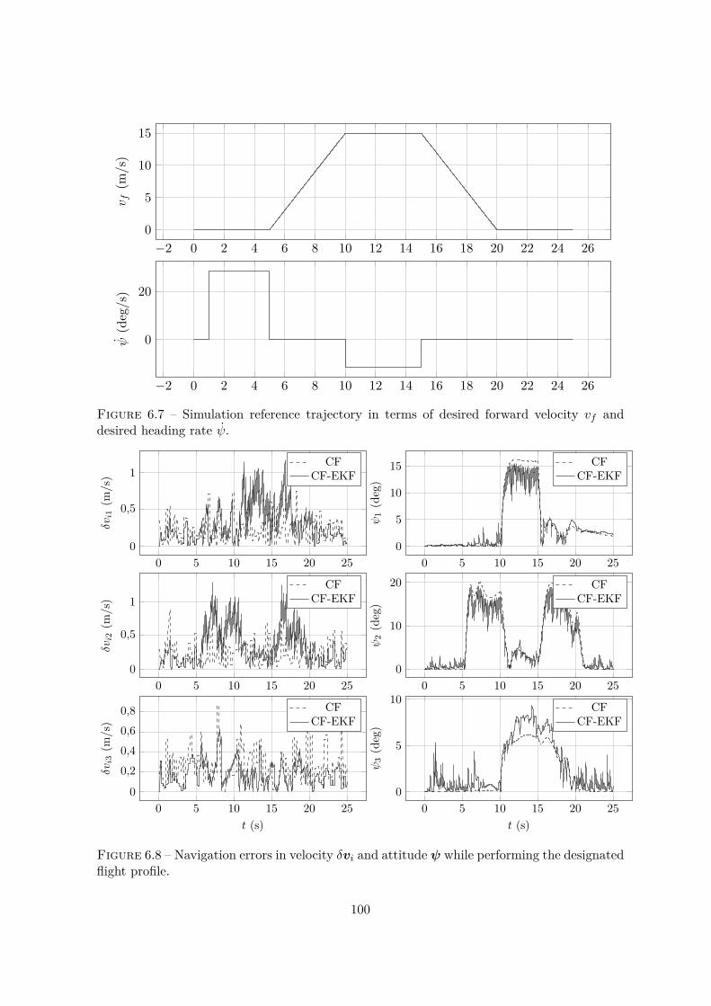
−2 0 2 4 6 8 10 12 14 16 18 20 22 24 260

5

10

15v f

(m/s)

−2 0 2 4 6 8 10 12 14 16 18 20 22 24 26

0

20

ψ(deg/s)

Figure 6.7 – Simulation reference trajectory in terms of desired forward velocity vf anddesired heading rate ψ.

0 5 10 15 20 250

0,5

1

δvi1

(m/s)

CFCF-EKF

0 5 10 15 20 250

0,5

1

δvi2

(m/s)

CFCF-EKF

0 5 10 15 20 250

0,20,40,60,8

t (s)

δvi3

(m/s)

CFCF-EKF

0 5 10 15 20 250

5

10

15

ψ1(deg)

CFCF-EKF

0 5 10 15 20 250

10

20

ψ2(deg)

CFCF-EKF

0 5 10 15 20 250

5

10

t (s)

ψ3(deg)

CFCF-EKF

Figure 6.8 – Navigation errors in velocity δvi and attitude ψ while performing the designatedflight profile.

100

Chapitre 7

Flight simulation and flight testing

Sommaire7.1 Introduction . . . . . . . . . . . . . . . . . . . . . . . . . . . . . . . . . . 1017.2 Flight simulations . . . . . . . . . . . . . . . . . . . . . . . . . . . . . . . 1017.3 Flight experiments . . . . . . . . . . . . . . . . . . . . . . . . . . . . . . . 1027.4 Concluding remarks . . . . . . . . . . . . . . . . . . . . . . . . . . . . . . 103

7.1 Introduction

By means of simulation and real flight experiments, the present chapter aims towardsvalidation of the gain-scheduled LQR controller previously designed in Chap. 5. Beforehand,the typical behavior of a single LQR (tuned for hovering flight) controller during a flighttransition maneuver is shown by means of simulations and real flights. Its shortcomings willbe shown to render transition flight impractical and the previously designed gain-scheduledcontroller is applied instead to stabilize the maneuver. The chosen estimation and controlstrategy is summarized in Fig. 7.1.

7.2 Flight simulations

The velocity v flight profile pursued by simulation is illustrated in Fig. 7.2. Notice thatvelocity is slowly increased by increments of 1m/s to prove stability in several points in themiddle of the transition.

Before simulating the full scheduled controller system, it is worth questioning whethergain-scheduling is really necessary. This question is supported by the fact that fixed-wingsare inherently stable 1 and therefore maybe a hover-stabilizing controller would also be suitablefor cruise mode. Fig. 7.2 illustrates the results of such a scenario. Notice that while hover isstable as expected, transition flight above 10m/s is unstable. Other choices for Q and R gainswere examined but yielded similar results. Finally, the instability in δi is in agreement with

1. Assuming that the fixed-wing was designed to be passively stable by choosing adequate center of massposition.

101

Velocityreference

Gainscheduler

LQR Actuatorsmodel

MAVionx = f(x,u)

vf , ψ xr +−

∆x

K,xr,ur

u∗ u x

Magnetometer

IMU

GNSS receiver

ComplementaryFilter

Mux

qv

Figure 7.1 – Block diagram of the MATLAB/Simulink simulation setup for the experiment.

our physical intuition of the system since elevons become more aerodynamically efficient (i.e.,an increase of Cmδ) in cruise flight due to the increase of wind.

The scheduled controller, on the other hand and as expected, stabilizes the system for anyvelocity as Fig. 7.3 shows. Furthermore, notice by means of propeller response ωi that systemtime constants are kept also constant over all velocities, while time constants are degraded inFig. 7.2 as velocity increases.

7.3 Flight experiments

Flight tests were conducted to investigate the predicted aforementioned velocity instabilitylimit due to single LQR control design. Fig. 7.4 illustrates an attempt for transition flight.Indeed, notice that every time vehicle velocity v rises above 10m/s, unstable pitch dynamicsappears (notice pronounced Q, δ1 and δ2 undamped oscillations). Therefore, the single LQRcontroller design is only able to stabilize the vehicle up to 10m/s. As it happens, this limitis below the optimal cruise velocity (see Chap. 3), and a different control design approach iscalled for. Finally, physically speaking, the instability on Q, δ1 and δ2 suggests that elevonsare more aerodynamic efficient during cruise flight, and a successful stabilizing control lawrequires that propulsion/aerodynamics interactions are accounted for.

As previously discussed, this thesis employs gain-scheduling LQR control design for achie-ving full flight envelope stabilization. Fig. 7.5 shows a successful attempt of flight transition.Notice that oscillations are no longer present, the cruise velocity was achieved and a back-to-hover maneuver was successfully performed.

102

7.4 Concluding remarks

This final chapter closes the case study by employing φ-theory to predict instability modesand successfully design a gain-scheduling controller – tuned in simulation and validated in realflights – to allow for safe TBV preliminary operation without resorting to long and exhaustingcontroller tuning campaigns.

103

0 5 10 15 20 25 30 35 40 45 50−5

0

5

10

15Speed limit

v(m

/s)

HorizontalVertical

0 5 10 15 20 25 30 35 40 45 50−400

−200

0

200

400

600

Instability!

ωb(deg/s)

P (ωb1)Q(ωb2)R(ωb3)

0 5 10 15 20 25 30 35 40 45 50−200

−100

0

100

200

Euler angles singularityθ,φ(deg)

φθ

0 5 10 15 20 25 30 35 40 45 50

4 000

5 000

ωi(R

PM)

ω1ω2

0 5 10 15 20 25 30 35 40 45 50−40

−20

0

20

40

Instability!

δ i(deg)

δ1δ2

Figure 7.2 – Flight simulation results with a single LQR controller.

104

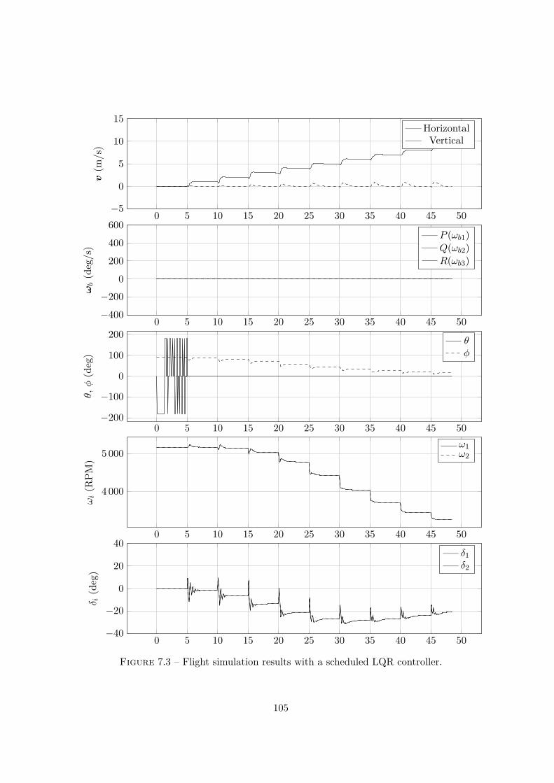
0 5 10 15 20 25 30 35 40 45 50−5

0

5

10

15 Speed limit

v(m

/s)

HorizontalVertical

0 5 10 15 20 25 30 35 40 45 50−400

−200

0

200

400

600

Instability!

ωb(deg/s)

P (ωb1)Q(ωb2)R(ωb3)

0 5 10 15 20 25 30 35 40 45 50−200

−100

0

100

200

θ,φ(deg)

θφ

0 5 10 15 20 25 30 35 40 45 50

4 000

5 000

ωi(R

PM)

ω1ω2

0 5 10 15 20 25 30 35 40 45 50−40

−20

0

20

40

Instability!

δ i(deg)

δ1δ2

Figure 7.3 – Flight simulation results with a scheduled LQR controller.

105

140 145 150 155 160 165 170 175−5

0

5

10

15 Speed limit

v(m

/s)

HorizontalVertical

140 145 150 155 160 165 170 175−400

−200

0

200

400

600

Instability!

ωb(deg/s)

P (ωb1)Q(ωb2)R(ωb3)

140 145 150 155 160 165 170 175−50

0

50

θ,φ(deg)

θφ

140 145 150 155 160 165 170 175

6 000

8 000

ωi(R

PM)

ω1ω2

140 145 150 155 160 165 170 175−40

−20

0

20

40

Instability!

δ i(deg)

δ1δ2

Figure 7.4 – Flight experiment results with a single LQR controller.

106

170 172 174 176 178 180 182 184 186−5

0

5

10

15Critical region

v(m

/s)

HorizontalVertical

170 172 174 176 178 180 182 184 186−200

−100

0

100

200

Stable!

ωb(deg/s)

P (ωb1)Q(ωb2)R(ωb3)

170 172 174 176 178 180 182 184 186

−50

0

50Stable!

θ,φ(deg)

θφ

170 172 174 176 178 180 182 184 1865 000

6 000

7 000

8 000Stable!

ωi(R

PM)

ω1ω2

170 172 174 176 178 180 182 184 186

−20

0

20

40

δ i(deg)

δ1δ2

Figure 7.5 – Flight experiment results with gain-scheduled LQR controllers.

107

Conclusion and perspectives

This study set out to establish a tractable model for tail-sitting vehicles in view of algorith-mic control design and qualitative dynamics analysis. The proposed φ-theory not only yields anumerically advantageous model but also extends our comprehension of tail-sitting vehicles.For instance, I have shown that propeller-wing interaction by an induced angle-of-attackconcept is equivalent to a constant thrust deflection under mild assumptions. Additionally,I have extensively explored the longitudinal quasi-static transition – which is often misun-derstood – and discussed the isolated nature of trim points. In sharp contrast with existentliterature, the proposed model is globally non-singular, polynomial-like and bypasses the useof aerodynamic angles α and β (both free-stream and propwash-induced).

Even if intellectually elegant, a mathematical model has practical use only if consistentwith reality. I show this is the case by means of wind tunnel and flight test experiments. Istrongly believe φ-theory provides a fitting balance between model complexity and controllerdesign simplicity. I prove this point by tuning our controller in simulation – by means of a thin-airfoil-based model with no specific airfoil aerodynamic data – and test-flying it (longitudinaland lateral maneuvers) in reality without resorting to further exhausting experimental tuningcampaigns, in sharp contrast to most existing literature. This is particularly convenient forlarger-scale TBVs and I am happy that the present work attracted the attention of industrialand academic partners in the region of Toulouse. Additionally, the proposed piloting interfaceallows flight at a continuous range of velocities (instead of the commonplace plane/hoverswitching philosophy that creates a velocity-deadzone) and results in increased robustness inview of tailwind, headwind and crosswind disturbances.

With a reliable model at hand, this work sets forth numerous exciting research possibi-lities. While I focused on model structure and properties – and thus provided but a simplecontroller for flight test validation – our findings suggest several courses of action for controllaw improvement. For instance, φ-theory forces and moments model remarkable simplicity al-lows for straightforward nonlinear inverse dynamics control studies that are known to provideimproved levels of performance in view of large state and control perturbations. Additionally,the proposed elliptical drag polar concept is practical for describing aerodynamics uncertain-ties in a powerful graphic method that transcribes uncertainties to parameters for µ-analysisand H∞ control design. Notice, for instance, that an arbitrary drag polar can be boundedbetween two φ-theory elliptical drag polars.

While φ-theory has been herein validated only for tail-sitting flying-wings, it shows greatpotential for describing arbitrary configurations. Further research might explore qualitativehandling quantities and stability of unfamiliar platforms (e.g., tilt-wings, tilt-motors, quad-copters with wings). Additionally, φ-theory could support the design of novel flight simulatorsfor inexperienced pilots in unfamiliar platforms – or even familiar platforms though in unfa-miliar conditions (e.g., high-maneuverable vehicles).

Tail-sitters pose a beautiful challenge and I hope the present work renders tail-sitters more

109

accessible to the underactuated robotics and control systems communities.

110

Annexe A

Falling leaf example data

The parameters employed for simulating the falling leaf example in Sec. 2.1.3 are givenby (A.1) and Table A.1.

Φ =

1.1310 −.9699 −.3505 −.0110 .0138 −.0273−.9699 3.1813 .6343 .0291 −.0088 .0149−.3505 .6343 .3318 .0400 −.0034 .0263−.0110 .0291 .0400 .0091 .0019 .0001.0138 −.0088 −.0034 .0019 .0026 −.0033−.0273 .0149 .0263 .0001 −.0033 .0146

(A.1)

Table A.1 – Falling leaf simulation parameters

Physical parameters Initial conditionsc 1 (m) Dl

b(0) I3b 1 (m) vb(0) [0 0 0]T (m/s)S 1 (m2) ωb(0) [0 0 0]T (rad/s)m 10 (g)J 0.004I3 (kg m2)g 9.81 (m/s2)ρ 1.225 (kg/m3)

111

Bibliographie

[Abe+14] D. Abeywardena et al. « Model-aided state estimation for quadrotor micro airvehicles amidst wind disturbances ». In : 2014 IEEE/RSJ International Confe-rence on Intelligent Robots and Systems (IROS 2014). 2014 (cf. p. 9).

[Abr+12] N. Abramov et al. « Pushing ahead — SUPRA airplane model for upset reco-very ». In : AIAA Modeling and Simulation Technologies Conference. 2012 (cf.p. 8).

[Alh+16] P. A. Alheritiere et al. « Nonlinear control of a particular tilt-body MAV :the Roll and Fly ». In : 2016 24th Mediterranean Conference on Control andAutomation (MED). 2016 (cf. p. 11, 54).

[Alz+15] H. Alzu’bi et al. « Evaluation of an aerial quadcopter power-plant for underwateroperation ». In : 2015 10th International Symposium on Mechatronics and itsApplications (ISMA). 2015 (cf. p. 6).

[AM90] B. D. O. Anderson et J. B. Moore. Optimal control : linear quadratic methods.Sous la dir. de Mineola. Dover, 1990 (cf. p. 65, 72, 73).

[And10] J. D. Anderson. Fundamentals of aerodynamics. McGraw-Hill, 2010 (cf. p. 17,30, 32).

[Asm63] F. J. Asmus. « Design and development of the tip turbine lift fan ». In : Annalsof the New York Academy of Sciences 107.1 (1963), p. 147–176 (cf. p. 5).

[Bat+09] B. Bataillé et al. « Development of a VTOL mini UAV for multi-tasking mis-sions ». In : The Aeronautical Journal 113.1140 (2009), p. 87–98 (cf. p. 53).

[BM95] F. Bullo et R. Murray. « Proportional derivative (PD) control on the Eucli-dean group ». In : Report or Paper (Technical Report), California Institute ofTechnology, CaltechCDSTR :1995.CIT-CDS-95-010. 1995 (cf. p. 8).

[Bor63] H. V. Borst. « Design and development considerations of the X-19 VTOL air-craft ». In : Annals of the New York Academy of Sciences 107 (1963), p. 265–279(cf. p. 5).

[BRK99] R. R. Burridge, A. A. Rizzi et D. E. Koditschek. « Sequential composition ofdynamically dexterous robot behaviors ». In : International Journal of RoboticsResearch 18.6 (1999), p. 534–555 (cf. p. 61).

[BSLK01] Y. Bar-Shalom, X. R. Li et T. Kirubarajan. Estimation with applicationsto tracking and navigation : theory, algorithms and software. Wiley-Interscience,2001 (cf. p. 94).

[Bur+15] M. Burri et al. « Robust state estimation for micro aerial vehicles based onsystem dynamics ». In : 2015 IEEE International Conference on Robotics andAutomation (ICRA). 2015 (cf. p. 9).

113

[Bye85] R. Byers. Numerical condition of the algebraic Riccati equation, Linear Algebraand its role in system theory. Sous la dir. de RI : AMS Contemporary MathematicsSeries. T. 47. Providence, 1985 (cf. p. 73).

[Car+17] M. Carrión et al. « Study of hybrid air vehicle stability using computationalfluid dynamics ». In : Journal of Aircraft 2017.4 (2017), p. 1328–1339 (cf. p. 8).

[CCS13] P. Casau, D. Cabecinhas et C. Silvestre. « Hybrid control strategy for theautonomous transition flight of a fixed-wing aircraft ». In : IEEE Transactionson Control Systems Technology 21.6 (2013) (cf. p. 58).

[Cho+11] A. Cho et al. « Wind estimation and airspeed calibration using a UAV with asingle-antenna GPS receiver and pitot tube ». In : IEEE Transactions on Aeros-pace and Electronic Systems 47 (2011), p. 109–117 (cf. p. 9).

[Chu+15] A. Chulliat et al. The US/UK World Magnetic Model for 2015-2020. Publica-tion - Report. BGS et NOAA, 2015 (cf. p. 93).

[CHW88] H.-D. Chiang, M. W. Hirsh et F. F. Wu. « Stability regions of nonlinear auto-nomous dynamical systems ». In : IEEE Transactions on Automatic Control 33.1(1988), p. 16–27 (cf. p. 60).

[CT08] R. Cory et R. Tedrake. « Experiments in fixed-wing UAV perching ». In :AIAA Guidance, Navigation and Control Conference and Exhibit. 2008 (cf. p. 18,43).

[CYB11] J. Calusdian, X. Yun et E. Bachmann. « Adaptive-gain complementary filterof inertial and magnetic data for orientation estimation ». In : 2011 IEEE In-ternational Conference on Robotics and Automation (ICRA). 2011, p. 1916–1922(cf. p. 88).

[Dic+07] J. Dickeson et al. « Robust LPV H∞ gain-scheduled hover-to-cruise conver-sion for a tiltwing rotorcraft in the presence of CG variations ». In : 46th IEEEConference on Decision and Control. 2007 (cf. p. 6).

[DVS17] Y. Demitrit, S. Verling et T. Stastny. « Model-based wind estimation fora hovering VTOL tailsitter UAV ». In : 2017 IEEE International Conference onRobotics and Automation (ICRA). 2017 (cf. p. 9).

[Ern+12] P. Ern et al. « Wake-induced oscillatory paths of bodies freely rising or falling influids ». In : Annual Review of Fluid Mechanics 44 (2012), p. 97–121 (cf. p. 25).

[Eus+08] M. Euston et al. « A complementary filter for attitude estimation of a fixed-wing UAV ». In : IEEE/RSJ International Conference on Intelligent Robots andSystems (IROS). 2008, p. 340–345 (cf. p. 88).

[Fay63] C. B. Fay. « A cursory analysis of the VTOL tilt-wing performance and controlproblems ». In : Annals of the New York Academy of Sciences 107 (1963), p. 102–146 (cf. p. 5).

[FB98] J. A. Farrell et M. Barth. The global positioning system and inertial naviga-tion. McGraw-Hill, 1998 (cf. p. 96).

114

[Fin+10] C. C. Finlay et al. « International geomagnetic reference field : the eleventhgeneration ». In : Geophysical Journal International 183.3 (2010), p. 1216–1230(cf. p. 93).

[Fis95] D. Fischenberg. « Identification of an unsteady aerodynamic stall model fromflight test data ». In : 20th Atmospheric Flight Mechanics Conference. 1995 (cf.p. 8).

[FL96] Y. Fan et F. Lutze. « Identification of an unsteady aerodynamic model at highangles of attack ». In : 21st Atmospheric Flight Mechanics Conference. 1996 (cf.p. 8).

[FMH02] R. Franz, M. Milam et J. Hauser. « Applied receding horizon control of theCaltech ducted fan ». In : American Control Conference. 2002 (cf. p. 9).

[Fra+07] A. Frank et al. « Hover, transition, and level flight control design for a single-propeller indoor airplane ». In : AIAA Guidance, Navigation, and Control Confe-rence and Exhibit. 2007 (cf. p. 18).

[Fri+17] N. T. Frink et al. « Computational aerodynamic modeling tools for aircraft lossof control ». In : Journal of Guidance, Control, and Dynamics 40.4 (2017), p. 789–803 (cf. p. 8).

[GA11] P. Gahinet et P. Apkarian. « Decentralized and fixed-structure H∞ control inMATLAB ». In : Proc. IEEE Conference on Decision and Control. 2011, p. 8205–8210 (cf. p. 58).

[GE63] P. F. Girard et W. L. Everett. « A test pilot report on the X-13 Vertijetand VZ-3RY vertiplane ». In : Annals of the New York Academy of Sciences 107(1963), p. 409–427 (cf. p. 5).

[Gil+13] S. J. Gill et al. « Upset dynamics of an airliner model : a nonlinear bifurcationanalysis ». In : Journal of Aircraft 50.6 (2013), p. 1832–1842 (cf. p. 8).

[Gil+15] S. J. Gill et al. « Nonlinear dynamics of aircraft controller characteristics outsidethe standard flight envelope ». In : Journal of Guidance, Control, and Dynamics38.12 (2015), p. 2301–2308 (cf. p. 8).

[GK94] M. Goman et A. Khrabrov. « State-space representation of aerodynamic cha-racteristics of an aircraft at high angles of attack ». In : Journal of Aircraft 31.5(1994), p. 1109–1115 (cf. p. 8).

[GMBI90] D. Goshen-Meskin et I. Y. Bar-Itzhack. « Observability analysis of piece-wise constant systems with application to inertial navigation ». In : 29th IEEEConference on Decision and Control. 1990, p. 821–826 (cf. p. 88).

[GMBI92] D. Goshen-Meskin et I. Y. Bar-Itzhack. « Observability analysis of piecewiseconstant systems. II. Application to inertial navigation in-flight alignment ». In :IEEE Transactions on Aerospace and Electronic Systems 28.4 (1992), p. 1068–1075 (cf. p. 88).

[Gre04] D. Greenwell. « A review of unsteady aerodynamic modelling for flight dyna-mics of manoeuvrable aircraft ». In : AIAA Atmospheric Flight Mechanics Confe-rence and Exhibit. 2004 (cf. p. 8).

115

[GSS93] N. J. Gordon, D. J. Salmond et A. F. M. Smith. « Novel approach to nonlinear/non-Gaussian Bayesian state estimation ». In : IEE Proceedings F - Radar and SignalProcessing 140.2 (1993), p. 107–113 (cf. p. 88).

[Hal+17] L. E. Hale et al. « Aerodynamic parameter identification and uncertainty quan-tification for small unmanned aircraft ». In : Journal of Guidance, Control, andDynamics 40.3 (2017), p. 680–691 (cf. p. 7).

[HBG14] G. Hattenberger, M. Bronz et M. Gorraz. « Using the Paparazzi UAVsystem for scientific research ». In : International Micro Air Vehicle Conferenceand Competition. 2014 (cf. p. 55).

[HDB16] K. Harikumar, S. Dhall et M. S. Bhat. « Nonlinear modeling and control ofcoupled dynamics of a fixed wing micro air vehicle ». In : 2016 Indian ControlConference (ICC). 2016 (cf. p. 8).

[HDH04] M. Heller, R. David et J. Holmberg. « Falling leaf motion suppression inthe F/A-18 Hornet with revised flight control software ». In : AIAA AerospaceSciences Meeting. 2004 (cf. p. 25).

[Hig75] W. T. Higgins. « A comparison of complementary and Kalman filtering ». In :IEEE Transactions on Aerospace and Electronic Systems (1975) (cf. p. 88).

[Hig88] N. Higham. « Computing a nearest symmetric positive semidefinite matrix ».In : Linear Algebra and its Applications 103 (1988), p. 103–118 (cf. p. 30).

[HMM17] P. Hartmann, C. Meyer et D. Moormann. « Unified velocity control andflight state transition of unmanned tilt-wing aircraft ». In : Journal of Guidance,Control, and Dynamics 40.6 (2017), p. 1348–1359 (cf. p. 7, 49).

[Ita+01] M. Itasse et al. « Equilibrium transition study for a hybrid MAV ». In : Inter-national Journal of Micro Air Vehicles 3 (2001), p. 229–245 (cf. p. 45).

[Joh00] T. A. Johansen. « Computation of Lyapunov functions for smooth nonlinearsystems using convex optimization ». In : Automatica 36.11 (2000), p. 1617–1626(cf. p. 58).

[JR96] P. T. Jaramillo et J. N. Ralston. « Simulation of the F/A-18D falling leaf ».In : AIAA Atmospheric Flight Mechanics Conference. 1996, p. 756–766 (cf. p. 25).

[JT07] D. Jung et P. Tsiotras. « Inertial attitude and position reference system deve-lopment for a small UAV ». In : In AIAA Infotech @ Aerospace 2007 Conferenceand Exhibit. 2007 (cf. p. 88).

[KSK17] H. Kang, J. Shen et A. R. Kreshock. « Validation of comprehensive analysis fortiltrotor whirl flutter predictions ». In : Journal of Aircraft 54.4 (2017), p. 1566–1570 (cf. p. 9).

[Kun05] D. L. Kunz. « Analysis of proprotor whirl flutter : review and update ». In :Journal of Aircraft 42.1 (2005), p. 172–178 (cf. p. 9).

[KZW17] M. Kuang, J. Zhu et W. Wang. « Flight controller design and demonstrationof a thrust-vectored tailsitter ». In : 2017 IEEE International Conference onRobotics and Automation (ICRA). 2017 (cf. p. 7).

116

[Lau78] A. J. Laub. A Schur method for solving algebraic Riccati equations. Rapp. tech.859. Massachussets Institute of Technology, Laboratory for Information et Deci-sion systems, LIDS, 1978 (cf. p. 66, 73).

[LDM14] L. R. Lustosa, F. Defay et J. M. Moschetta. « Development of the flightmodel of a tilt-body MAV ». In : International Micro Air Vehicle Conference andCompetition. 2014 (cf. p. 11).

[LDM15] L. R. Lustosa, F. Defay et J. M. Moschetta. « Longitudinal study of a tilt-body vehicle : modeling, control and stability analysis ». In : International Confe-rence on Unmanned Aircraft Systems. 2015 (cf. p. 11, 53, 58).

[LDM17] L. R. Lustosa, F. Defay et J. M. Moschetta. « The feasibility issue in tra-jectory tracking by means of regions-of-attraction-based gain scheduling ». In :IFAC 2017 World Congress. 2017 (cf. p. 11).

[LDMde] L. R. Lustosa, F. Defay et J. M. Moschetta. « The φ-theory approach to tail-sitting algorithmic flight control – Part I : Modeling ». In : Journal of Guidance,Control, and Dynamics ((under review)) (cf. p. 11).

[Lei06] J. G. Leishman. Principles of helicopter aerodynamics. Cambridge UniversityPress, 2006 (cf. p. 32).

[LGW17] X. Lyu, H. Gu et Y. Wang. « Design and implementation of a quadrotor tail-sitter VTOL UAV ». In : 2017 IEEE International Conference on Robotics andAutomation (ICRA). 2017 (cf. p. 6–8).

[Lus+16] L. R. Lustosa et al. « An error model of a complementary filter for use in Baye-sian estimation - The CF-EKF filter ». In : 20th IFAC Symposium on AutomaticControl in Aerospace. 2016 (cf. p. 11).

[Lus+17] L. R. Lustosa et al. « Team MAVion entry in the IMAV’17 outdoor challenge– A tail-sitting trajectory tracking µUAV ». In : International Micro Air VehicleConference and Competition. 2017 (cf. p. 11).

[May79] P. S. Maybeck. Stochastic models, estimation, and control. Academic Press, 1979(cf. p. 96).

[McC98] B. W. McCormick. Aerodynamics of V/STOL flight. Dover publications, 1998(cf. p. 32, 33).

[MCT14] J. Moore, R. Cory et R. Tedrake. « Robust post-stall perching with a simplefixed-wing glider using LQR-trees ». In : Bioinspiration and Biomimetics 9.2(2014) (cf. p. 9, 58).

[MHD15] M. W. Mueller, M. Hehn et R. D’Andrea. « A computationally efficient mo-tion primitive for quadrocopter trajectory generation ». In : IEEE Transactionson Robotics 31.6 (2015), p. 1294–1310 (cf. p. 10).

[MHP05] R. Mahony, T. Hamel et J. M. Pflimlin. « Complementary filter design onthe special orthogonal group SO(3) ». In : Proc. IEEE Conf. Decision Control.2005, p. 1477–1484 (cf. p. 88).

117

[MLD14] J. M. Moschetta, L. R. Lustosa et F. Defay. « On the design of hybrid microair vehicles for multi-tasking missions ». In : 2nd AETOS international conferenceon Research challenges for future RPAS/UAV systems. 2014 (cf. p. 11).

[MO09] D. K. K. Muraoka et N. Okada. « Quad tilt wing VTOL UAV : Aerodynamiccharacteristics and prototype flight ». In : AIAA Infotech Aerospace Conference.2009 (cf. p. 6).

[Mor17] E. A. Morelli. « Dynamic modeling from flight data with unknown time skews ».In : Journal of Guidance, Control, and Dynamics 40.8 (2017), p. 2084–2092 (cf.p. 7).

[MSD15] M. M. Maia, P. Soni et F. J. Diez. « Demonstration of an aerial and submer-sible vehicle capable of flight and underwater navigation with seamless air-watertransition ». In : The Computing Research Repository (CoRR). 2015 (cf. p. 6).

[MST11] C. G. Mayhew, R. G. Sanfelice et A. R. Teel. « Quaternion-based hybridcontrol for robust global attitude tracking ». In : IEEE Transactions on AutomaticControl 56.11 (2011) (cf. p. 58).

[MST13] C. G. Mayhew, R. G. Sanfelice et A. R. Teel. « On path-lifting mechanismsand unwinding in quternion-based attitude control ». In : IEEE Transactions onAutomatic Control 58.5 (2013) (cf. p. 59).

[MT12] J. Moore et R. Tedrake. « Control synthesis and verification for a perchingUAV using LQR-trees ». In : IEEE Conference on Decision and Control. 2012(cf. p. 59).

[Neu+12] P. P. Neumann et al. « Autonomous gas-sensitive microdrone : wind vector esti-mation and gas distribution mapping ». In : Robotics and Automation Magazine19.1 (2012), p. 50–61 (cf. p. 9).

[Oos+13] A. Oosedo et al. « Development of a quad rotor tail-sitter VTOL UAV withoutcontrol surfaces and experimental verification ». In : 2013 IEEE InternationalConference on Robotics and Automation (ICRA). 2013 (cf. p. 6).

[Par00] P. A. Parrilo. « Structured semidefinite programs and semialgebraic geometrymethods in robustness and optimization ». Thèse de doct. California Institute ofTechnology, 2000 (cf. p. 58).

[PCK91] P. Petkov, N. Christov et M. Konstantinov. Computational methods forlinear control systems. Sous la dir. de New York : Prentice. New York : Prentice,1991 (cf. p. 66, 73).

[Pen+13] L. Peng et al. « Adaptive proprotors as applied to convertible MAVs ». In :International Micro Air Vehicle Conference and Flight Competition. 2013 (cf.p. 54).

[PHS07] J. M. Pflimlin, T. Hamel et P. Soueres. « Nonlinear attitude and gyroscope’sbias estimation for a VTOL UAV ». In : International Journal of Systems Science38.3 (2007), p. 197–210 (cf. p. 88).

118

[PL03] P. A. Parrilo et S. Lall. « Semidefinite programming relaxations and algebraicoptimization in control ». In : European Journal of Control 9.2-3 (2003), p. 307–321 (cf. p. 18, 25).

[PLG13] J. Pattinson, M. H. Lowenberg et M. G. Goman. « Investigation of poststallpitch oscillations of an aircraft wind-tunnel model ». In : Journal of Aircraft 50.6(2013), p. 1843–1855 (cf. p. 8).

[Poi08] D. Poinsot. « Commande d’un drone en vue de la conversion vol rapide - volstationnaire ». Thèse de doct. ISAE-SUPAERO, 2008 (cf. p. 81).

[PPB07] D. Poinsot, A. Piquereau et C. Berard. « Optimisation des transitions dephases de vol pour un drone capable de vol stationnaire et de vol en translationrapide ». In : Journées Nationales MACS. 2007 (cf. p. 81).

[PTD17] R.-A. Peloquin, D. Thibault et A. L. Desbiens. « Design of a passive verticaltakeoff and landing aquatic UAV ». In : IEEE Robotics and Automation Letters2.2 (2017), p. 381–388 (cf. p. 7).

[Puc13] Daniele Pucci. « Towards an unified approach for the control of aerial vehicles ».Thèse de doct. Universite de Nice-Sophia Antipolis, Sapienza Universita di Roma,2013 (cf. p. 7).

[RD17] R. Ritz et R. D’Andrea. « A global controller for flying wing tailsitter vehicles ».In : 2017 IEEE International Conference on Robotics and Automation (ICRA).2017 (cf. p. 7, 8).

[Rei+11] G. W. Reich et al. « Transient poststall aerodynamic modeling for extreme ma-neuvers in micro air vehicles ». In : Journal of Aircraft 48.2 (2011), p. 403–411(cf. p. 8).

[SA77] M. G. Safonov et M. Athans. « Gain and phase margins for multiloop LQGregulators ». In : IEEE Transactions on Automatic Control (1977) (cf. p. 65).

[SBM08] S. Shkarayev, B. Bataille et J. M. Moschetta. « Aerodynamic design ofmicro air vehicles for vertical flight ». In : Journal of Aircraft 45.5 (2008), p. 1715–1724 (cf. p. 36, 53).

[Sch+14] F. Schiano et al. « Towards estimation and correction of wind effects on a qua-drotor UAV ». In : IMAV 2014 : International Micro Air Vehicle Conference andCompetition. 2014 (cf. p. 9).

[Sch16] D. K. Schmidt. « Stability augmentation and active flutter suppression of aflexible flying-wing drone ». In : Journal of Guidance, Control, and Dynamics39.3 (2016), p. 409–422 (cf. p. 9).

[Sch63] C. F. Schmidt. « Flight safety in VTOL aircraft ». In : Annals of the New YorkAcademy of Sciences 107 (1963), p. 3–469 (cf. p. 5).

[SCW16] L. N. C. Sikkel, G. C. H. E. de Croon et C. De Wagter. « A novel onlinemodel-based wind estimation approach for quadrotor micro air vehicles using lowcost MEMS IMUs ». In : 2016 IEEE/RSJ International Conference on IntelligentRobots and Systems (IROS). 2016 (cf. p. 9).

119

[SH09] F. M. Sobolic et J. P. How. « Nonlinear agile control test bed for a fixed-wingaircraft in a constrained environment ». In : AIAA Infotech Aerospace Conference.2009 (cf. p. 18).

[Sin+12] P. Sinha et al. « Versatile, modular, extensible VTOL aerial platform with au-tonomous flight mode transitions ». In : 2012 IEEE Aerospace Conference. 2012(cf. p. 6).

[Sin+13] M. Sinha et al. « High angle of attack parameter estimation of cascaded finsusing neural network ». In : Journal of Aircraft 50.1 (2013), p. 272–291 (cf. p. 8).

[SJ96] J. Singh et R. V. Jategaonkar. « Identification of lateral-directional behaviorin stall from flight data ». In : Journal of Aircraft 33.3 (1996), p. 627–630 (cf.p. 8).

[SL03] B. L. Stevens et F. L. Lewis.Aircraft control and simulation. Wiley-Interscience,2003 (cf. p. 12, 13, 93, 94).

[SM15] M. Sato et K. Muraoka. « Flight controller design and demonstration of quad-tilt-wing unmanned aerial vehicle ». In : Journal of Guidance, Control, and Dy-namics 38.6 (2015), p. 1071–1082 (cf. p. 6, 7).

[SM16] M. Sato et K. Muraoka. « Flight controller design for small quad tilt wingUAV ». In : Journal of the Japan Society for Aeronautical and Space Sciences64.1 (2016), p. 79–82 (cf. p. 6, 7).

[Sme+14] E. J. J. Smeur et al. « Modelling of a hybrid UAV using test flight data ». In :International Micro Air Vehicle Conference and Competition. 2014 (cf. p. 7).

[Ted+10] R. Tedrake et al. « LQR-trees : feedback motion planning via sums of squaresverification ». In : International Journal of Robotics Research 29 (2010), p. 1038–1052 (cf. p. 58, 61).

[The+17] B. Theys et al. « Experimental and numerical study of micro-aerial-vehicle pro-peller performance in oblique Flow ». In : Journal of Aircraft 54.3 (2017), p. 1076–1084 (cf. p. 9, 39).

[TM17] P. Tsiotras et M. Mesbahi. « Toward an algorithmic control theory ». In :Journal of Guidance, Control, and Dynamics 40.2 (2017), p. 194–196 (cf. p. 9).

[Top+10] U. Topcu et al. « Robust region-of-attraction estimation ». In : IEEE Transac-tions on Automatic Control 55.1 (2010), p. 137–142 (cf. p. 60).

[Tot+16] H. Totoki et al. « Design and testing of a low-order flight control system forquad-tilt-wing UAV ». In : Journal of Guidance, Control, and Dynamics 39.10(2016), p. 2426–2433 (cf. p. 5).

[TP08] W. Tan et A. Packard. « Stability region analysis using polynomial and com-posite polynomial Lyapunov functions and sum-of-squares programming ». In :IEEE Transactions on Automatic Control 53.2 (2008), p. 565–571 (cf. p. 60).

[TP09] U. Topcu et A. Packard. « Local stability analysis for uncertain nonlinearsystems ». In : IEEE Transactions on Automatic Control 54.5 (2009), p. 1042–1047 (cf. p. 60).

120

[TSK17] Y. H. Tan, R. Siddall et M. Kovac. « Efficient aerial–aquatic locomotion witha single propulsion system ». In : IEEE Robotics and Automation Letters 2.3(2017), p. 1304 –1311 (cf. p. 6).

[US17] D. V. Uhlig et M. S. Selig. « Modeling micro air vehicle aerodynamics in uns-teady high angle-of-attack flight ». In : Journal of Aircraft 54.3 (2017), p. 1064–1075 (cf. p. 8).

[Val+13] E. R. Valeria et al. « LQR control for a quadrotor using unit quaternions :modeling and simulation ». In : 2013 International Conference on Electronics,Communications and Computing (CONIELECOMP). 2013, p. 172–178 (cf. p. 59).

[Vas+09] J. F. Vasconcelos et al. « Discrete time-varying attitude complementary fil-ter ». In : Proc. American Control Conference. 2009, p. 4056–4061 (cf. p. 88).

[VC+16] J. Velasco-Carrau et al. « Multi-objective optimization for wind estimationand aircraft model identification ». In : Journal of Guidance, Control, and Dy-namics 39.2 (2016), p. 372–389 (cf. p. 9).

[VSB17] S. Verling, T. Stastny et G. Bättig. « Model-based transition optimizationfor a VTOL tailsitter ». In : 2017 IEEE International Conference on Roboticsand Automation (ICRA). 2017 (cf. p. 6, 9).

[WBI78] A. Weinred et I. Y. Bar-Itzhack. « The psi-angle error equation in strapdowninertial navigation systems ». In : IEEE Aerospace and Electronic Systems AES-14.3 (1978), p. 539–542 (cf. p. 88).

[WD91] J. T. Y. Wen et K. K. Delgado. « The attitude control problem ». In : IEEETransactions on automatic control 36.10 (1991) (cf. p. 58).

[WW09] S. Waslander et C. Wang. « Wind disturbance estimation and rejection forquadrotor position control ». In : AIAA Infotech at Aerospace Conference. 2009(cf. p. 9).

[Yan+15] X. Yang et al. « Survey on the novel hybrid aquatic-aerial amphibious air-craft : aquatic unmanned aerial vehicle (AquaUAV) ». In : Progress in AerospaceSciences 74 (2015), p. 131–151 (cf. p. 7).

[Yan16] Y. Yang. « Controllability of spacecraft using only magnetic torques ». In : IEEETransactions on Aerospace and Electronic Systems 52.2 (2016) (cf. p. 59, 73, 74).

[çe+11] E. çetonsoy et al. « Design and development of a tilt-wing UAV ». In : TurkishJournal of Electrical Engineering and Computer Sciences 19.5 (2011), p. 733–741(cf. p. 6).

121

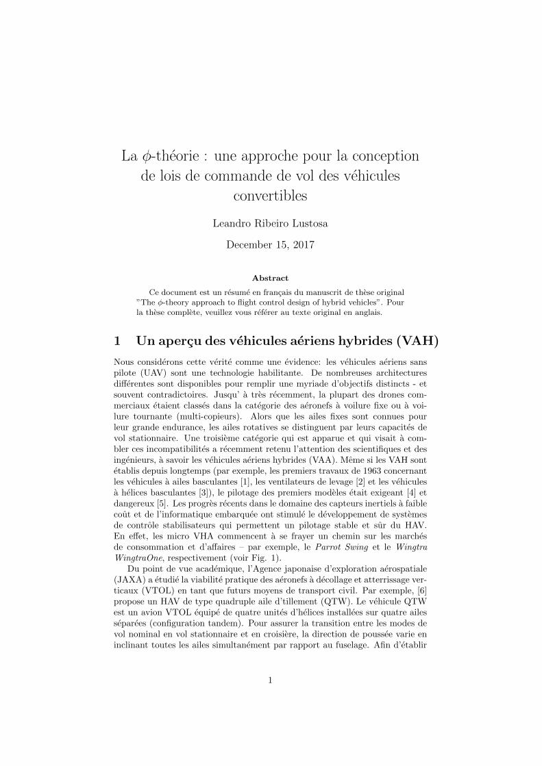
La φ-theorie : une approche pour la conception

de lois de commande de vol des vehicules

convertibles

Leandro Ribeiro Lustosa

December 15, 2017

Abstract

Ce document est un resume en francais du manuscrit de these original”The φ-theory approach to flight control design of hybrid vehicles”. Pourla these complete, veuillez vous referer au texte original en anglais.

1 Un apercu des vehicules aeriens hybrides (VAH)

Nous considerons cette verite comme une evidence: les vehicules aeriens sanspilote (UAV) sont une technologie habilitante. De nombreuses architecturesdifferentes sont disponibles pour remplir une myriade d’objectifs distincts - etsouvent contradictoires. Jusqu’ a tres recemment, la plupart des drones com-merciaux etaient classes dans la categorie des aeronefs a voilure fixe ou a voi-lure tournante (multi-copieurs). Alors que les ailes fixes sont connues pourleur grande endurance, les ailes rotatives se distinguent par leurs capacites devol stationnaire. Une troisieme categorie qui est apparue et qui visait a com-bler ces incompatibilites a recemment retenu l’attention des scientifiques et desingenieurs, a savoir les vehicules aeriens hybrides (VAA). Meme si les VAH sontetablis depuis longtemps (par exemple, les premiers travaux de 1963 concernantles vehicules a ailes basculantes [1], les ventilateurs de levage [2] et les vehiculesa helices basculantes [3]), le pilotage des premiers modeles etait exigeant [4] etdangereux [5]. Les progres recents dans le domaine des capteurs inertiels a faiblecout et de l’informatique embarquee ont stimule le developpement de systemesde controle stabilisateurs qui permettent un pilotage stable et sur du HAV.En effet, les micro VHA commencent a se frayer un chemin sur les marchesde consommation et d’affaires – par exemple, le Parrot Swing et le WingtraWingtraOne, respectivement (voir Fig. 1).

Du point de vue academique, l’Agence japonaise d’exploration aerospatiale(JAXA) a etudie la viabilite pratique des aeronefs a decollage et atterrissage ver-ticaux (VTOL) en tant que futurs moyens de transport civil. Par exemple, [6]propose un HAV de type quadruple aile d’tillement (QTW). Le vehicule QTWest un avion VTOL equipe de quatre unites d’helices installees sur quatre ailesseparees (configuration tandem). Pour assurer la transition entre les modes devol nominal en vol stationnaire et en croisiere, la direction de poussee varie eninclinant toutes les ailes simultanement par rapport au fuselage. Afin d’etablir

1

(a) Up-start (Airborne Concept) (b) Swing (Parrot) (c) WingtraOne (Wingtra)

Figure 1: Commercial examples of HAVs.

des techniques de guidage et de controle QTW, JAXA a developpe deux pro-totypes miniaturises de QTW [7, 8]. De plus, JAXA a confirme la faisabilitedu vol de transition au moyen de controleurs de vol bases sur le gain. D’autresexemples d’aile inclinee incluent la [9, 10, 11].

Une simplification (mecaniquement parlant) de la conception quadruple d’aileest la carrosserie quadruple d’aile, ou le fuselage du vehicule tourne de maniererigide avec l’aile [12]. Parmi les etudes interessantes, on peut citer [13] qui pro-pose un corps quadruple a balancier permettant d’obtenir un atterrissage stableen stationnaire et fiable en cas de perturbation par le vent jusqu’ a 5,2 m/s.Il est interessant de noter qu’il a egalement conclu que, meme si les ailettesdiedres contribuent dans une certaine mesure au vol a l’horizontale, elles creenten quelque sorte des couples avec un niveau important de nuisance causee parle vent de travers. De plus, si le lecteur a deja vu le Parrot Swing sur le marche,une caracteristique qui frappe l’œil est sa configuration de rotors inclines (ilsne sont pas paralleles comme dans la plupart des quadrotors). [13] soutientque ce choix de conception dans les quadruplets est choisi pour maximiser lebras moteur et donc augmenter les moments de roulis induits par la poussee dumoteur afin de surmonter les perturbations dues au vent pendant le vol stati-onnaire (surtout si des ailettes sont presentes). Dans les avions, la stabilite vaa l’encontre de la manoeuvrabilite (p. ex., les chasseurs sont intrinsequementinstables pour favoriser la manoeuvrabilite); dans la conception du VAH, la sta-bilite en vol vers l’avant peut egalement entraıner une perturbation accrue duvol stationnaire. S’opposer aux choix de conception dans differents modes estun probleme recurrent et represente un defi supplementaire pour la conceptionHAV. [14], alternativement, inclut deux elevons a la conception quadruple-tilt-corps pour atteindre des degres supplementaires d’actionnement et attenuer lememe probleme.

Une autre approche de conception HAV est l’aile volante arriere [15]. Cetteconception favorise la simplicite en minimisant les pieces mobiles (pas de mo-teurs ou d’ailes basculantes). Au lieu de cela, une configuration approprieede moteur tandem avec aile et deux elevateurs fournit, en termes simples, uneaile volante capable de supporter un vol stationnaire. Par rapport aux corpsquadruple-til, il necessite moins de volume et favorise ainsi la miniaturisationet l’utilisation dans la construction de missions d’intrusion.

Enfin, je termine la vue d’ensemble du paysage avec des plates-formes plusexotiques, mais dont les defis technologiques sont lies a ceux qui ont ete discutesprecedemment. Un premier exemple est celui des vehicules aeriens-aquatiques

2

[16, 17]. [18], par exemple, decrit une aile volante a helice unique capabled’effectuer un vol a voilure fixe et une locomotion d’immersion. Pour augmenterles performances, une boıte de vitesses bimode est utilisee pour obtenir unelocomotion air-aquatique econergetique efficace avec une seule helice. De meme,[19] fournit une aile volante capable de decoller et d’atterrir verticalement surl’eau. Un resume des vehicules aeriens-aquatiques est decrit dans [20].

2 HAV modelisation et controle de conceptionetat de l’art

A la connaissance de l’auteur, le pilote automatique Pixhawk est actuellementle seul systeme open source a implementer les lois de controle du HAV. Lesregulateurs de vol stationnaire et de croisiere y sont utilises separement en tantque regulateurs traditionnels multi helicopteres et a voilure fixe. Au cours d’unetransition, ceux-ci sont interchanges et un algorithme de melange ad hoc tente delisser les transitions transitoires resultantes. Il vaut la peine de noter, cependant,que le commentaire suivant (que mon experience appuie fermement) a affiche lanote de bas de page 1 dans leur site Web HAV: ”La base de code actuelle ouvrela voie aux applications VTOL, mais elle en est encore a ses debuts. En cemoment, vous aurez probablement besoin d’une bonne comprehension de la basede code PX4 et quelques competences de vol pour faire fonctionner la caipirinhaVTOL avec succes. Nous mettons beaucoup d’efforts dans le developpement dela base de code VTOL”. Des exemples recents d’une telle strategie de transitionde controle de vol se trouvent dans [21]. [21] a la particularite de changernon seulement les lois de controle mais aussi la definition des angles Euler afind’eviter les singularites d’attitude. Cependant, la plupart des autres travauxutilisent le quaternion comme parametrage d’attitude global (et numeriquementstable).

Cette these poursuit une approche similaire a celle de la [22, 23, 13], pourlaquelle le vol de transition n’est pas considere comme une transition transi-toire temporaire (et en quelque sorte indesirable) entre les modes de vol, maiscomme un mode de vol fonctionnel en soi. De ce point de vue, le pilote est enmesure de stabiliser le vehicule a un ensemble continu de vitesses en marcheavant de zero (rotation) a la vitesse de croisiere nominale. Il est de la responsa-bilite du controleur d’abstraire les ordres de velocite pour obtenir des referencesd’assiette et d’actionneur adequates, meme si cela signifie qu’il faut stabiliseraux angles d’attaque posterieurs a la mise en place. Ceci confirme l’utilite d’unemodelisation adequate apres la pose.

Du point de vue de la modelisation HAV pour la conception des commandes,par exemple, [22] utilise des tables de recherche obtenues au moyen de longuescampagnes statiques en soufflerie pour concevoir des controleurs programmes engain sans avoir recours a un modele mathematique analytique. Une approchesimilaire est utilisee dans [7, 8]. D’autre part, [13] ajuste les donnees de souf-flerie a une formule de coefficient aerodynamique donnee en fonction de l’angled’attaque α pour obtenir des modeles analytiques. De plus, les coefficientsdynamiques necessitent des campagnes de soufflerie encore plus complexes oudes instruments de vol complexes [24]. Si l’instrumentation a faible cout est

1Vendredi 25 aout 2017,14 h 40 (GMT+2) @ pixhawk.org/platforms/vtol/tbs caipirinha vtol.

3

appliquee et que la synchronisation des donnees est prohibitive, les travauxrecents [25] propose une methode d’identification dynamique des coefficients apartir des donnees de vol avec des biais d’horloge (horodatage) inconnus. Deplus, il va sans dire que l’identification parametrique n’est pas la seule place dansla modelisation. [26] traite (et fournit des methodes de mesure) des incertitudesdues a la forme supposee du modele algebrique des coefficients aerodynamiques.Une contribution interessante – etroitement liee a la philosophie de conduite queje vais suivre ici – se trouve dans [27]. Dans celui-ci, la structure algebrique ducoefficient aerodynamique est limitee a une famille de fonctions soigneusementchoisies pour promouvoir la conception globale de controle non lineaire. Danscette these, cependant, je limite la structure des coefficients aerodynamiquespour promouvoir la conception de controle algorithmique.

Cette these utilise une approche a l’etat d’equilibre pour modeliser les coef-ficients aerodynamiques, c’est-a-dire que je neglige les processus dynamiques dedelestage des tourbillons [28], dans lesquels une augmentation rapide de l’angled’attaque provoque la formation d’un tourbillon de pointe qui produit une aug-mentation instable de la portance qui decroıt au fur et a mesure que le tour-billon est transporte en aval. Dans ce scenario, les coefficients aerodynamiquesdependent de l’historique des angles d’attaque et des derapages. Dans les tra-vaux precedents [29, 30, 31, 32, 33, 34, 35, 36], la modelisation est realisee aumoyen d’un etat du systeme augmente qui inclut un parametre de separationde flux. En poursuivant d’abord l’approche en regime permanent, je suis enmesure d’identifier quels sont les phenomenes HAV qualitatifs pouvant etre ca-racterises par cette approche simplifiee, et quels phenomenes necessitent dessystemes d’ordres augmentes.

Cette these utilise une approche a l’etat d’equilibre pour modeliser les coef-ficients aerodynamiques, c’est-a-dire que je neglige les processus dynamiques dedelestage des tourbillons [28], dans lesquels une augmentation rapide de l’angled’attaque provoque la formation d’un tourbillon de pointe qui produit une aug-mentation instable de la portance qui decroıt au fur et a mesure que le tour-billon est transporte en aval. Dans ce scenario, les coefficients aerodynamiquesdependent de l’historique des angles d’attaque et des derapages. Dans les tra-vaux precedents [29, 30, 31, 32, 33, 34, 35, 36], la modelisation est realisee aumoyen d’un etat du systeme augmente qui inclut un parametre de separationde flux. En poursuivant d’abord l’approche en regime permanent, je suis enmesure d’identifier quels sont les phenomenes HAV qualitatifs pouvant etre ca-racterises par cette approche simplifiee, et quels phenomenes necessitent dessystemes d’ordres augmentes.

Une autre approche pour traiter l’incertitude des coefficients aerodynamiquesconsiste a utiliser des lois de controle adaptatif. Par exemple, dans l’affaire [23],on a effectue des experiences en vol en utilisant des techniques d’apprentissagemachine pour estimer les parametres aerodynamiques du corps incline d’unmodele de principes fondamentaux et en adaptant le controleur en consequence.

Etant donne que les VHA ailes operent souvent dans les regions posterieuresa l’installation, on dispose rapidement de nombreuses connaissances dans la do-cumentation sur les pertes de maıtrise des aeronefs. Par exemple, [37] resumel’etat de la recherche en cours a la NASA pour faire progresser les modelesde simulation de vol augmentee pour les LOC d’aeronefs civils en raison dudecrochage des ailes a des fins de formation des pilotes. Cet article est par-ticulierement interessant, car il aborde le defi constant de creer des modeles

4

non lineaires a ordre reduit a partir de donnees informatiques haute fidelite etd’experiences en vol, qui constituent le fondement philosophique de la presentethese. J’aimerais egalement citer ici les remarques de [37] et leurs remarquessur les capacites actuelles de la dynamique des fluides numerique (CFD) comptetenu des differents regimes de vol: ”Apres huit annees de collaboration cibleeentre un corps international diversifie d’aerodynamiciens et d’experts en simu-lation de vol, la conclusion retentissante etait que, meme si la methodologieCFD actuelle permettait de predire facilement le comportement S&C[stabilite etcontrole] des aeronefs volant dans les regions lineaires d’une enveloppe de vol,il est toujours extremement difficile de saisir adequatement les caracteristiquesstatiques et dynamiques des flux non lineaires.” Neanmoins, des efforts recentsont ete deployes pour fournir une technique informatique de dynamique desfluides permettant de predire l’amortissement aerodynamique dynamique desVHA.

La plupart des controleurs a voilure fixe que l’on trouve dans la litteraturedecouplent la dynamique laterale et longitudinale de sorte que la modelisationet la conception des commandes se deroulent independamment l’une de l’autre.Cependant, [38] analyse les effets de couplage entre les dynamiques lateraleset longitudinales d’une aile volante gardienne et conclut que la dynamique despirale instable est incorrectement stabilisee par des hypotheses de decouplage.Cela donne a penser que la dynamique couplee est fondamentale pour les VHAet qu’il faut privilegier la conception des commandes a entrees multiples etsorties multiples (MIMO). [13], par exemple, utilise une commande en cascadecomposee de boucles externes MIMO non lineaires d’angle stable exponentiel[39] et de boucles angulaires PID internes MIMO.

Avec l’avancee des systemes informatiques embarques rapides et fiables, latheorie du controle algorithmique [40] a ete mise en evidence ces dernieresannees. Cette theorie s’ecarte du controleur de structure algebrique fixe habi-tuel pour s’eloigner d’un mappage etat-erreur-actionneur implicitement calculepar un algorithme (souvent convexe de resolution d’optimisation). Parmi lesexemples recents lies aux VHA, citons la [41, 42]. La presente these promeutcette ligne de pensee en fournissant - en plus d’autres caracteristiques - desmodeles dynamiques de VHA optimises et faciles a resoudre. En plus de laconception des commandes, les techniques d’optimisation permettent une iden-tification efficace des modeles aerodynamiques, comme dans [43], ou une techni-que est proposee pour l’estimation du vent apres le vol en l’absence de capteursde donnees atmospheriques. Une fois la vitesse du vent estimee, les donneesde vol sont corrigees et utilisees pour estimer le coefficient aerodynamique. Jenote que, si des routines d’optimisation efficaces sont disponibles, cette memetechnique peut etre appliquee en temps reel pour la compensation des perturba-tions dues au vent en vol. Alors que le tube de Pitot est instrumental pour lesailes fixes [44], la large enveloppe d’angle d’attaque trouvee sur les corps bas-culants empeche leur utilisation, et des techniques comme celle qui vient d’etrementionnee sont de la plus haute necessite. A la connaissance de l’auteur, cedernier est le seul ouvrage sur l’estimation du vent a bord des corps basculants.Les travaux anterieurs sur l’estimation du vent basee sur des modeles pour lesmulti-copieurs en vol stationnaire sont les suivants: [45, 46, 47, 48, 49, 50].

De plus, la plupart des equations differentielles de modele HAV actuellessont immensement generales, sans structure particuliere qui pourrait etre ex-ploitee dans des solutions d’optimisation specialisees. [15], par exemple, utilise

5

un outil d’optimisation polyvalent pour rechercher des trajectoires de croisiereet de survol de la caisse basculante tout en optimisant une certaine fonction decout. La presente these vise cependant a modeliser les VHA a partir des prin-cipes de la physique et des restrictions algebriques pour obtenir des systemessans singularite qui possedent une structure speciale en vue d’une optimisationefficace (et donc en temps reel).

Bien que la modelisation des helices a ecoulement oblique soit fondamentalepour l’analyse des performances de vol, sa pertinence pour la conception descommandes de retroaction est discutable. De plus, la modelisation de l’incidencedes helices est complexe et necessite souvent des campagnes en soufflerie. Parexemple, [51] montre que, bien que la combinaison traditionnelle de la theoriede l’element de pale, de la methode du reseau tourbillonnaire et de la theoriede l’elan pour l’ecoulement oblique soit un outil courant pour la conceptiond’helicopteres, elle ne reflete pas correctement les donnees de soufflerie dans lesangles d’incidence eleves.

Enfin, je n’ai pas ressenti le besoin de prendre en compte les modes dyna-miques structuraux flexibles tout en developpant la partie experimentale pourle drone particulier de l’ISAE, et je renvoie le lecteur a [52] pour une etude decas recente sur l’aile volante flexible. Je remarque que, meme si je crois queles effets de flexibilite ne representent pas un probleme dans la conception descommandes de vol nominales du HAV, ils definissent le vol nominal lui-meme.[53, 54] reconnaissent que la vitesse de croisiere et l’autonomie sont limiteesdirectement ou indirectement par la stabilite structurale du rotor d’helice, dupylone et de l’aile.

3 Motivation de these

Pour mieux comprendre ce qui m’ a pousse a m’ecarter des forces aerodynamiquestraditionnelles et des parametrisations des moments dans cette these, il faut te-nir compte des tendances actuelles dans la conception des commandes. Uneconference inspirante de Bode2 dans la Conference de 2016 sur le controle et ladecision, donnee par le professeur Richard Murray, predit les orientations futu-res de la recherche sur la conception des controles. Il a affirme que la facon dontnous synthetisons et pensons aux controleurs de feed-forward et de feedbackchange d’une maniere similaire a la facon dont nous effectuons d’autres calculs(simplifies).

Par exemple, songez a calculer les racines d’un polynome du deuxieme or-dre. De telles racines sont facilement disponibles grace a la formule de Bhaskara.Cependant, pour les plus grands degres polynomiaux, une formule generale estprouvee inexistante, et notre solution actuelle est de la calculer numeriquementau moyen d’algorithmes (dans lesquels la reponse du probleme n’est pas ob-tenue par une formule analytique mais, au lieu de cela, par un nombre finid’iterations d’une recette d’approximation pour obtenir un resultat de precisionarbitraire). Un autre exemple est la solution de systemes lineaires d’ordre elevedes equations. Meme avec les formules analytiques disponibles pour les systemesde n’importe quel ordre, un ordinateur numerique est capable de trouver dessolutions beaucoup plus rapidement au moyen d’algorithmes numeriques.

2Lecture: Future directions in control: a look backwards and forwards, disponible en lignesur le site de l’IEEE: http://www.ieeecss-oll.org/category/lecture-type/bode-lecture.

6

De meme, jusqu’ a recemment, les controleurs etaient mis en œuvre unique-ment a partir de formules analytiques des erreurs de reference estimees d’etat oude sortie. Cependant, une tendance recente propose implicitement de calculerles actions des actionneurs au moyen d’algorithmes numeriques, generalementpar le biais de programmes d’optimisation (qui, en outre, sont une facon natu-relle de decrire les problemes de controle). C’est en train de devenir une realiteet elle est illustree par des copies multiples tres adroites dans [55]. Toutefois, cestechniques ne sont pas encore appliquees dans les VHA en raison de l’absencede modeles mathematiques appropries. Les solveurs d’optimisation efficaces ex-igent une sorte de structure dans le modele mathematique du vehicule, et lesmodeles HAV d’aujourd’hui sont beaucoup trop generaux pour convenir a laplupart des solveurs de maniere efficace (et donc en temps reel).

Cette these fournit une structure de modele appropriee adaptee aux besoinsd’optimisation en ligne, mais suffisamment complexe pour decrire toutes les sub-tilites du vol HAV. Je crois que ce modele de these ouvre la voie a d’importantespossibilites interessantes en matiere de generation et de controle des trajectoiresde VHA, et j’espere rendre les VHA plus accessibles aux communautes generalesde controle et de robots.

4 Feuille de route pour la these

4.1 Enonce du probleme

Je poursuis une description mathematique de la dynamique des vols de transi-tion sous forme non lineaire x = f(x,u) telle que (i) f(·) est polynomiale et doncsingularite libre sur toute la configuration. (ii) L’identification des parametresf(·) necessite des calculs pas de soufflerie ni de dynamique des fluides surordinateur pour concevoir un pilote automatique stable preliminaire; (iii) f(·)structure simple encourage la conception de retroaction non lineaire et une pla-nification/optimisation efficace de la retroaction avant; (iv) fournit du interieurdans la dynamique qualitative du vehicule et (v) peut etre valide au moyende campagnes en soufflerie et d’experiences de vol.

4.2 Contributions a la these

Contributions theoriques: Le cadre de travail φ-thory est propose pour lamodelisation des vehicules hybrides. Ses proprietes mathematiques et ses ca-racteristiques sont minutieusement etudiees. La presente these montre que lesmodeles fondes sur la theorie de φ concordent avec les points (i) a (iv) de lasection 4.1.

Contributions experimentales: Cette these met en contraste les donneesde soufflerie avec les resultats theoriques pour evaluer la pertinence de la theorieφ dans le monde reel. Les vols experimentaux font appel a des estimateursetatiques qui utilisent des capteurs de navigation a faible cout. Pour cela, lapresente these etudie une nouvelle architecture d’estimateur d’etat qui jette lesbases d’une navigation inertielle assistee qui utilise un filtrage complementairepour l’estimation de l’attitude au moyen d’un magnetometre comme aide ex-terne, et un EKF pour l’integration de capteurs supplementaires. Enfin, un

7

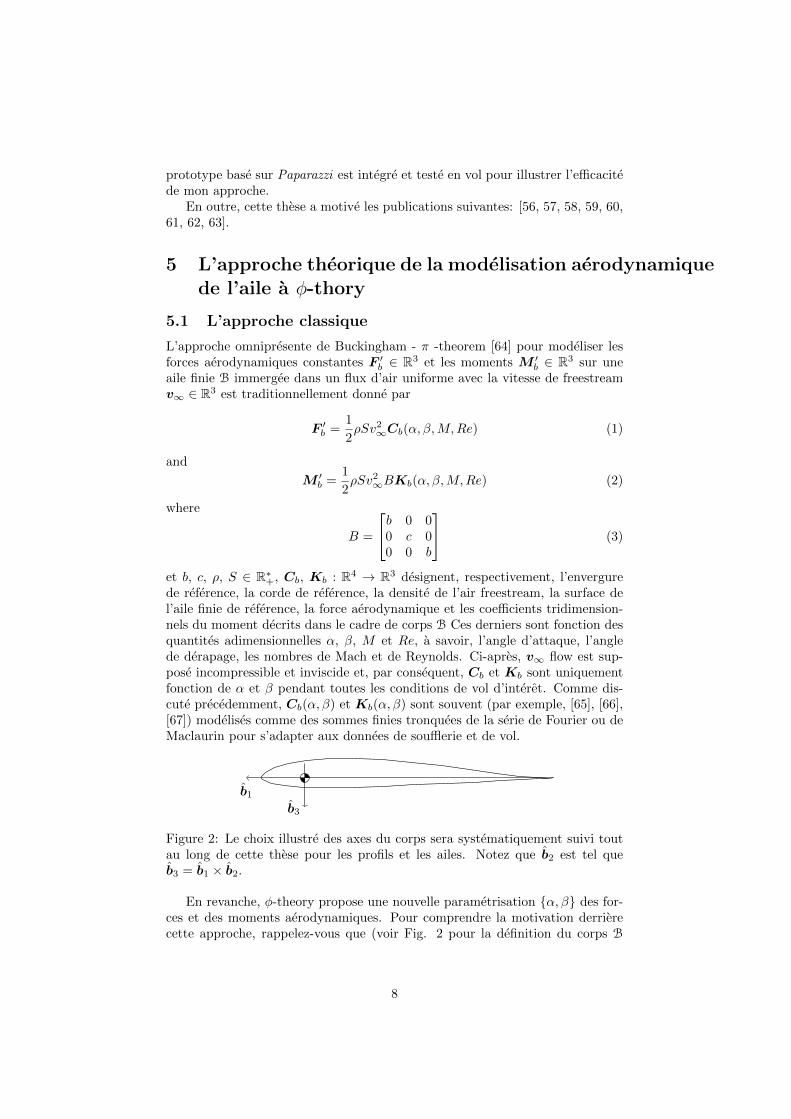
prototype base sur Paparazzi est integre et teste en vol pour illustrer l’efficacitede mon approche.

En outre, cette these a motive les publications suivantes: [56, 57, 58, 59, 60,61, 62, 63].

5 L’approche theorique de la modelisation aerodynamiquede l’aile a φ-thory

5.1 L’approche classique

L’approche omnipresente de Buckingham - π -theorem [64] pour modeliser lesforces aerodynamiques constantes F ′b ∈ R3 et les moments M ′

b ∈ R3 sur uneaile finie B immergee dans un flux d’air uniforme avec la vitesse de freestreamv∞ ∈ R3 est traditionnellement donne par

F ′b =1

2ρSv2

∞Cb(α, β,M,Re) (1)

and

M ′b =

1

2ρSv2

∞BKb(α, β,M,Re) (2)

where

B =

b 0 00 c 00 0 b

(3)

et b, c, ρ, S ∈ R∗+, Cb, Kb : R4 → R3 designent, respectivement, l’envergurede reference, la corde de reference, la densite de l’air freestream, la surface del’aile finie de reference, la force aerodynamique et les coefficients tridimension-nels du moment decrits dans le cadre de corps B Ces derniers sont fonction desquantites adimensionnelles α, β, M et Re, a savoir, l’angle d’attaque, l’anglede derapage, les nombres de Mach et de Reynolds. Ci-apres, v∞ flow est sup-pose incompressible et inviscide et, par consequent, Cb et Kb sont uniquementfonction de α et β pendant toutes les conditions de vol d’interet. Comme dis-cute precedemment, Cb(α, β) et Kb(α, β) sont souvent (par exemple, [65], [66],[67]) modelises comme des sommes finies tronquees de la serie de Fourier ou deMaclaurin pour s’adapter aux donnees de soufflerie et de vol.

b1

b3

Figure 2: Le choix illustre des axes du corps sera systematiquement suivi toutau long de cette these pour les profils et les ailes. Notez que b2 est tel queb3 = b1 × b2.

En revanche, φ-theory propose une nouvelle parametrisation {α, β} des for-ces et des moments aerodynamiques. Pour comprendre la motivation derrierecette approche, rappelez-vous que (voir Fig. 2 pour la definition du corps B

8

axes)

α = tan−1

(v∞,b3v∞,b1

)(4)

et

β = sin−1

(v∞,b2v∞

)(5)

Cependant, le vol en queue-de-queue et le vol tres manoeuvrable rencontrentdes vitesses quasi-nulles (principalement dans les sections d’aile non couvertespar le glissement des helices) qui appellent des divisions algebriques proches dezero (4) et empechent la stabilite numerique simulations numeriques. Bien queles instructions if-else avec des seuils ad hoc appropries resolvent le probleme,notez cependant que

∂α

∂v∞,b1= − v∞,b3

v2∞,b1 + v2

∞,b3(6)

et, par consequent, ∇α(v∞,b) n’est pas continue a v∞,b = 0 en raison de (6) etdonne un mappage non differentiable quelle que soit la valeur que l’on definitpour α aux singularites de (4). Cette propriete empeche l’emploi de techniquesde linearisation pour le controle et l’analyse pendant le vol stationnaire (danslequel le comportement α et β est extremement sensible sur les sections d’aileseche).

En outre, la presente these tente d’adapter les donnees experimentales localestout en recherchant simultanement un comportement global qualitatif satisfai-sant. Par exemple, notez qu’une queue-sitter en descente en vol stationnairerencontre un α = π extrinseque en vue de l’aerodynamique aerodynamiquetraditionnelle et exige des capacites coherentes d’extrapolation des coefficientsaerodynamiques.

Enfin, des efforts recents [68] en optimisation de programmation semidefi-nie (SDP) et de somme des carres (SOS) permettent une optimisation et uncontrole efficaces des trajectoires dans des modeles dynamiques regis par desequations differentielles polynomiales. La formulation traditionnelle des coeffi-cients aerodynamiques comporte des fonctions trigonometriques qui empechentl’emploi du SDP et appelle a des routines couteuses de planification de trajec-toires. Alternativement, φ-theory propose une formulation favorable au SDP.

5.2 La parametrisation φ-theory

La theorie φ est construite sur la parametrisation {α, β} suivante des forces etdes moments aerodynamiques:

τ = −1

2ρSηCΦ(η)Cη (7)

ou τ , η ∈ R6, η ∈ R+, sont respectivement le cle aerodynamique (par rapportau centre de masse), wing twist, et aerodynamique φ-norm donnee par

τb =

(FbMb

)(8)

ηb =

(v∞,bω∞,b

)(9)

9

etη =

√v2∞ + φc2ω2

∞, φ > 0 (10)

ou φ ∈ R∗+ est un parametre accordable sans dimension. De plus, ω∞,b inR3

denote la moitie de la vorticite libre ξ∞ telle que 3

ω∞ =1

2ξ∞ =

1

2∇× v∞ (11)

En l’absence de vent, on peut facilement prouver que ω∞ est egal a la vitesseangulaire du vehicule. De plus, la matrice de reference wing vis C ∈ R6×6 estune extension du concept de matrice de reference de l’aile et est definie comme

C =

[I3×3 03×3

03×3 B

](12)

Enfin, Φ : R6 → R6×6 est le aerodynamique φ -coefficient. Le symbole φest introduit dans la nomenclature pour faciliter les paralleles entre la nouvelleparametrisation et les coefficients / derives bases sur Buckingham - Π. De plus,par souci de brievete, les formules et coefficients Buckingham - Π (par exemple,CL, CD) sont references comme π textit -theory et π -coefficients dans ce quisuit, tandis que le modele actuel est reference comme φ -theory et φ -coefficients.

Sauf indication contraire, Φ(·) est considere comme une fonction constanteecrite comme

Φ =

[Φ(fv) Φ(fω)

Φ(mv) Φ(mω)

](13)

ou Φ(fv), Φ(fω), Φ(mv), Φ(mω) ∈ R3×3. On montrera que cette hypothese sim-plifie grandement le modele tout en captant les caracteristiques dominantes -p. Ex. Effets post-decrochage, derives aerodynamiques, dissipation globale del’energie - sur l’ensemble de l’enveloppe de vol (vol stationnaire, croisiere ettransition). modes).

Quelques resultats theoriques suivent pour soutenir l’emploi de la theorie φdans les applications a enveloppe large. Ensuite, un exemple de chute de feuillesillustre la theorie avant d’aborder cette these motivation principale, a savoir, leprobleme de l’inclinaison du corps. Les preuves de ces resultats peuvent etretrouvees dans le document de these complet.

Definition 5.1 (Systeme de corps en apesanteur) Soit B un corps rigided’inertie (m,J) sous l’influence de forces et de moments aerodynamiques dansun champ de gravite negligeable sans vent. Le Systeme de corps en apesanteur(WBS) est defini comme le systeme dynamique associe donne par

vb = 1mFb − [ωb×]vb

ωb = J−1Mb − J−1[ωb×]Jωb

τb = −ηΦηb

(14)

Definition 5.2 (Systeme de chute libre) Soit B un corps rigide avec iner-tie (m,J) par l’influence des forces aerodynamiques et des moments dans une

3ω∞ est defini au moyen de la vorticite par souci de clarte. Neanmoins, bien que fluide, leflux freestream constitue un mouvement rigide et on peut considerer ω∞ comme une vitesseangulaire libre.

10

constante (trame par inertielle L) champ gravitationnel gl 6= 0 sans vent. Lesysteme dynamique de chute libre (FFS) est defini comme le systeme dynamiqueassocie donne par

vb = 1mFb +Dl

bgl − [ωb×]vb

ωb = J−1Mb − J−1[ωb×]Jωb

Dlb = −[ωb×]Dl

b

τb = −ηΦηb

(15)

Definition 5.3 (Etats terminaux et vitesses terminales) L’ensemble de etatsterminaux T ⊂ R3 × R3 × SO(3) d’un systeme dynamique de chute libre estdefini comme

T = {(vb,ωb, Dlb) ∈ R3 × R3 × SO(3) : vb = 0, ωb = 0, Dl

b = 03×3} (16)

En consequence, l’ensemble de vitesses terminales Tv ⊂ R3 est defini commesuit:

Tv = {vb ∈ R3 : (vb,ωb, Dlb) ∈ T pour certains ωb, D

lb} (17)

Theorem 5.1 (Aerodynamique dissipative) Supposons un WBS avec desconditions initiales arbitraires vb(0),ωb(0) ∈ R3. Si Φ � 0, alors vb(t) → 0 etωb(t)→ 0 uniformement t→∞.

Notez que Theoreme 5.1 corrobore la coherence φ-theory dans les applica-tions a enveloppe large si l’on choisit Φ ∈ S6

++ (Sn++ l’ensemble des matricesdefinies positives dans Rn×n). Les cles aerodynamiques sont dissipatives dansla realite et Theorem 5.1 fournit une condition suffisante sur Φ pour atteindreV ≤ 0 globalement. De meme, les resultats suivants explorent des proprietessupplementaires φ-theory.

Lemma 5.1 (Geometrie des etats terminaux) Supposons un FFS avec Φ �0. Si Φ(mv) est le rang complet, alors T = ∅. Sinon, (v0,ω0, D0) ∈ T si et seu-lement si

ω0 = 0, v0 6= 0

v0 ∈ ker(Φ(mv))

v0 =√

2mgρS||Φ(fv)v0||

1||Φ(fv)v0||

Φ(fv)v0 = −D0gl

(18)

Corollary 5.1 Supposons un FFS avec Φ � 0. Tv est soit

1. vide, si rank(Φ(mv)) = 3;

2. un couple de points antipodaux, si rang(Φ(mv)) = 2;

3. une courbe planaire fermee dans R3, si rang(Φ(mv)) = 1;

4. une surface fermee dans R3, si rang(Φ(mv)) = 0.

La figure 3 illustre le corollaire 5.1. Remarquez comment les symetriesgeometriques influencent rank(Φ(mv)). Par exemple, la symetrie autour d’unpoint (ie une balle) suggere rank(Φ(mv)) = 0 alors que rank(Φ(mv)) = 1 evoque lasymetrie autour d’un axe (par exemple, un ellipsoıde). De plus, l’auteur suggere

11

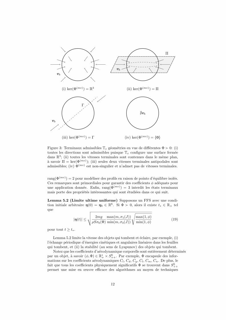
(i) ker(Φ(mv)) = R3

vb

Π

(ii) ker(Φ(mv)) = Π

vb

Γ

(iii) ker(Φ(mv)) = Γ

vb

(iv) ker(Φ(mv)) = {0}

@vb

Figure 3: Terminaux admissibles Tv geometries en vue de differentes Φ � 0: (i)toutes les directions sont admissibles puisque Tv configure une surface fermeedans R3; (ii) toutes les vitesses terminales sont contenues dans le meme plan,a savoir Π = ker(Φ(mv)); (iii) seules deux vitesses terminales antipodales sontadmissibles; (iv) Φ(mv) est non-singulier et n’admet pas de vitesses terminales.

rang(Φ(mv)) = 2 pour modeliser des profils en raison de points d’equilibre isoles.Ces remarques sont primordiales pour garantir des coefficients φ adequats pourune application donnee. Enfin, rang(Φ(mv)) = 3 interdit les etats terminauxmais porte des proprietes interessantes qui sont etudiees dans ce qui suit.

Lemma 5.2 (Limite ultime uniforme) Supposons un FFS avec une condi-tion initiale arbitraire η(0) = η0 ∈ R6. Si Φ � 0, alors il existe t∗ ∈ R+ telque

|η(t)| ≤

√√√√ 2mg

ρSσ6(Φ)

max(m,σ1(J))

min(m,σ3(J))

√max(1, φ)

min(1, φ)(19)

pour tout t ≥ t∗.

Lemma 5.2 limite la vitesse des objets qui tombent et eclaire, par exemple, (i)l’echange periodique d’energies cinetiques et angulaires lineaires dans les feuillesqui tombent, et (ii) la stabilite (au sens de Lyapunov) des objets qui tombent.

Notez que les coefficients d’aerodynamique corporelle sont entierement determinespar un objet, a savoir (φ,Φ) ∈ R∗+ × S6

++. Par exemple, Φ encapsule des infor-mations sur les coefficients aerodynamiques Cl, Cd, Cy, Cl, Cm, Cn. De plus, lefait que tous les coefficients physiquement significatifs Φ se trouvent dans S6

++

permet une mise en œuvre efficace des algorithmes au moyen de techniques

12

d’optimisation semi-definies positives [68]. De plus, les equations differentiellesdu corps rigide sont de type polynomial et invitent a l’optimisation SOS.

6 Experiences de soufflerie

Aussi elegant soit-il, un modele mathematique est peu pratique s’il n’est pascoherent avec la realite. Si elle est coherente avec la realite, la theorie φ fournitun modele convivial pour la conception de controle, effectue des vols d’essai etcollecte des donnees de vol en sautant la necessite des campagnes de soufflerie.Pour verifier si nous avons la coherence de la realite en utilisant φ -theory,une campagne en soufflerie a ete menee. Nous esperons que la consistanceconduira a des vols reussis, ce qui conduira a moins d’utilisation de la souffleriea l’avenir pour les conceptions de controle (bien sur, les campagnes en souffleriesont toujours inestimables pour la conception aerodynamique). Cet objectifprincipal de cette section est donc de comparer les points theoriques theoriquesde l’inclinaison par rapport aux donnees reelles de la soufflerie.

Les experiences ont ete conduites a la soufflerie en boucle fermee du sabre(Fig. 4) situee a l’ISAE et capable de fournir un flux stable et uniforme de faibleReynolds a une vitesse de vent de 2 a 25 m/s. ideal pour l’experimentation devehicules de micro-air a pleine portee (section d’essai de 2,4 m × 1,2m). Lesforces et les moments ont ete mesures au moyen d’une balance interne a 5composants etalonnee. La table 1 illustre la gamme (plutot inhabituelle) dedifferents parametres etudies au cours des experiences.

Figure 4: A gauche, sabre ( textit Soufflerie bas Reynolds) une soufflerie enboucle fermee. A droite, le modele de tunnel aerodynamique MAVion en coursde test.

v∞ 10 m/sα [−10, 90] degβ [0, 90] degωi [0, 8000] RPMδi [−30, 30] deg

Table 1: Les variables de vol ont ete testees en soufflerie.

13

References

[1] C. B. Fay. A cursory analysis of the VTOL tilt-wing performance andcontrol problems. Annals of the New York Academy of Sciences, 107:102–146, 1963.

[2] F. J. Asmus. Design and development of the tip turbine lift fan. Annals ofthe New York Academy of Sciences, 107(1):147–176, 1963.

[3] H. V. Borst. Design and development considerations of the X-19 VTOLaircraft. Annals of the New York Academy of Sciences, 107:265–279, 1963.

[4] P. F. Girard and W. L. Everett. A test pilot report on the X-13 vertijet andvz-3ry vertiplane. Annals of the New York Academy of Sciences, 107:409–427, 1963.

[5] C. F. Schmidt. Flight safety in VTOL aircraft. Annals of the New YorkAcademy of Sciences, 107:3–469, 1963.

[6] H. Totoki, Yoshimasa Ochi, Masayuki Sato, and Koji Muraoka. Design andtesting of a low-order flight control system for quad-tilt-wing uav. Journalof Guidance, Control, and Dynamics, 39(10):2426–2433, 2016.

[7] M. Sato and K. Muraoka. Flight controller design and demonstration ofquad-tilt-wing unmanned aerial vehicle. Journal of Guidance, Control, andDynamics, 38(6):1071–1082, 2015.

[8] M. Sato and K. Muraoka. Flight controller design for small quad tilt winguav. Journal of the Japan Society for Aeronautical and Space Sciences,64(1):79–82, 2016.

[9] E. cetonsoy, E. Sirimoglu, K. T. Oner, C. Hancer, M. Unel, M. F. Ak-sit, I. Kandemir, and K. Gulez. Design and development of a tilt-wingUAV. Turkish Journal of Electrical Engineering and Computer Sciences,19(5):733–741, 2011.

[10] D. K. K. Muraoka and N. Okada. Quad tilt wing VTOL UAV: Aerody-namic characteristics and prototype flight. In AIAA Infotech AerospaceConference, 2009.

[11] J. Dickeson, D. Miles, O. Cifdaloz, V. Wells, and A. Rodriguez. RobustLPV h∞ gain-scheduled hover-to-cruise conversion for a tiltwing rotorcraftin the presence of CG variations. In 46th IEEE Conference on Decisionand Control, 2007.

[12] A. Oosedo, S. Abiko, A. Konno, T. Koizumi, T. Furui, and M. Uchiyama.Development of a quad rotor tail-sitter vtol uav without control surfacesand experimental verification. In 2013 IEEE International Conference onRobotics and Automation (ICRA), 2013.

[13] X. Lyu, H. Gu, and Y. Wang. Design and implementation of a quadrotortail-sitter vtol uav. In 2017 IEEE International Conference on Roboticsand Automation (ICRA), 2017.

14

[14] P. Sinha, P. Esden-Tempski, C. A. Forrette, J. K. Gibboney, and G. M.Horn. Versatile, modular, extensible vtol aerial platform with autonomousflight mode transitions. In 2012 IEEE Aerospace Conference, 2012.

[15] S. Verling, T. Stastny, and G. Battig. Model-based transition optimizationfor a vtol tailsitter. In 2017 IEEE International Conference on Roboticsand Automation (ICRA), 2017.

[16] H. Alzu’bi, O. Akinsanya, N. Kaja, I. Mansour, and O. Rawashdeh. Eva-luation of an aerial quadcopter power-plant for underwater operation. In2015 10th International Symposium on Mechatronics and its Applications(ISMA), 2015.

[17] M. M. Maia, P. Soni, and F. J. Diez. Demonstration of an aerial and sub-mersible vehicle capable of flight and underwater navigation with seamlessair-water transition. In The Computing Research Repository (CoRR), 2015.

[18] Y. H. Tan, R. Siddall, and M. Kovac. Efficient aerial–aquatic locomotionwith a single propulsion system. IEEE Robotics and Automation Letters,2(3):1304 – 1311, 2017.

[19] R.-A. Peloquin, D. Thibault, and A. L. Desbiens. Design of a passivevertical takeoff and landing aquatic uav. IEEE Robotics and AutomationLetters, 2(2):381–388, 2017.

[20] X. Yang, T. Wang, J. Liang, G. Yao, and M. Liu. Survey on the novelhybrid aquatic-aerial amphibious aircraft: aquatic unmanned aerial vehicle(aquauav). Progress in Aerospace Sciences, 74:131–151, 2015.

[21] M. Kuang, J. Zhu, and W. Wang. Flight controller design and demonstra-tion of a thrust-vectored tailsitter. In 2017 IEEE International Conferenceon Robotics and Automation (ICRA), 2017.

[22] P. Hartmann, C. Meyer, and D. Moormann. Unified velocity control andflight state transition of unmanned tilt-wing aircraft. Journal of Guidance,Control, and Dynamics, 40(6):1348–1359, 2017.

[23] R. Ritz and R. D’Andrea. A global controller for flying wing tailsitter vehi-cles. In 2017 IEEE International Conference on Robotics and Automation(ICRA), 2017.

[24] E. J. J. Smeur, Q. P. Chu, G. C. H. E. De Croon, B. Remes, C. De Wagter,and E. Van der Horst. Modelling of a hybrid uav using test flight data. InInternational Micro Air Vehicle Conference and Competition, 2014.

[25] E. A. Morelli. Dynamic modeling from flight data with unknown timeskews. Journal of Guidance, Control, and Dynamics, 40(8):2084–2092,2017.

[26] L. E. Hale, Mayuresh Patil, , and Christopher J Roy. Aerodynamic pa-rameter identification and uncertainty quantification for small unmannedaircraft. Journal of Guidance, Control, and Dynamics, 40(3):680–691, 2017.

15

[27] Daniele Pucci. Towards an unified approach for the control of aerial vehi-cles. PhD thesis, Universite de Nice-Sophia Antipolis, Sapienza Universitadi Roma, 2013.

[28] D. V. Uhlig and M. S. Selig. Modeling micro air vehicle aerodynamics inunsteady high angle-of-attack flight. Journal of Aircraft, 54(3):1064–1075,2017.

[29] M. Goman and A. Khrabrov. State-space representation of aerodynamiccharacteristics of an aircraft at high angles of attack. Journal of Aircraft,31(5):1109–1115, 1994.

[30] Y. Fan and F. Lutze. Identification of an unsteady aerodynamic model athigh angles of attack. In 21st Atmospheric Flight Mechanics Conference,1996.

[31] D. Fischenberg. Identification of an unsteady aerodynamic stall model fromflight test data. In 20th Atmospheric Flight Mechanics Conference, 1995.

[32] J. Singh and R. V. Jategaonkar. Identification of lateral-directional beha-vior in stall from flight data. Journal of Aircraft, 33(3):627–630, 1996.

[33] M. Sinha, R. Ayilliath Kuttieri, Ajoy Kanti Ghosh, and Ajay Misra. Highangle of attack parameter estimation of cascaded fins using neural network.Journal of Aircraft, 50(1):272–291, 2013.

[34] G. W. Reich, F. E. Eastep, Aaron Altman, and Roberto Albertani. Tran-sient poststall aerodynamic modeling for extreme maneuvers in micro airvehicles. Journal of Aircraft, 48(2):403–411, 2011.

[35] J. Pattinson, M. H. Lowenberg, and M. G. Goman. Investigation of poststallpitch oscillations of an aircraft wind-tunnel model. Journal of Aircraft,50(6):1843–1855, 2013.

[36] D. Greenwell. A review of unsteady aerodynamic modelling for flight dy-namics of manoeuvrable aircraft. In AIAA Atmospheric Flight MechanicsConference and Exhibit, 2004.

[37] N. T. Frink, Patrick C. Murphy, Harold L. Atkins, Sally A. Viken, Justin L.Petrilli, Ashok Gopalarathnam, and Ryan C. Paul. Computational aero-dynamic modeling tools for aircraft loss of control. Journal of Guidance,Control, and Dynamics, 40(4):789–803, 2017.

[38] K. Harikumar, S. Dhall, and M. S. Bhat. Nonlinear modeling and control ofcoupled dynamics of a fixed wing micro air vehicle. In 2016 Indian ControlConference (ICC), 2016.

[39] F. Bullo and R. Murray. Proportional derivative (pd) control on the eucli-dean group. In Report or Paper (Technical Report), California Institute ofTechnology, CaltechCDSTR:1995.CIT-CDS-95-010, 1995.

[40] P. Tsiotras and M. Mesbahi. Toward an algorithmic control theory. Journalof Guidance, Control, and Dynamics, 40(2):194–196, 2017.

16

[41] R. Franz, M. Milam, and J. Hauser. Applied receding horizon control ofthe Caltech ducted fan. In American Control Conference, 2002.

[42] J. Moore, R. Cory, and R. Tedrake. Robust post-stall perching with asimple fixed-wing glider using LQR-trees. Bioinspiration and Biomimetics,9(2), 2014.

[43] J. Velasco-Carrau, S. Garcıa-Nieto, J. V. Salcedo, and R. H. Bishop. Multi-objective optimization for wind estimation and aircraft model identifica-tion. Journal of Guidance, Control, and Dynamics, 39(2):372–389, 2016.

[44] A. Cho, J. Kim, S. Lee, , and C. Kee. Wind estimation and airspeedcalibration using a uav with a single-antenna gps receiver and pitot tube.IEEE Transactions on Aerospace and Electronic Systems, 47:109–117, 2011.

[45] L. N. C. Sikkel, G. C. H. E. de Croon, and C. De Wagter. A novel onlinemodel-based wind estimation approach for quadrotor micro air vehiclesusing low cost mems imus. In 2016 IEEE/RSJ International Conferenceon Intelligent Robots and Systems (IROS), 2016.

[46] M. Burri, M. Datwiler, M. W. Achtelik, and R. Siegwart. Robust stateestimation for micro aerial vehicles based on system dynamics. In 2015IEEE International Conference on Robotics and Automation (ICRA), 2015.

[47] P. P. Neumann, S. Asadi, A. J. Lilienthal, M. Bartholmai, and J. H. Schil-ler. Autonomous gas-sensitive microdrone: wind vector estimation and gasdistribution mapping. Robotics and Automation Magazine, 19(1):50–61,2012.

[48] D. Abeywardena, Z. Wang, G. Dissanayake, S. L. Waslander, and S. Ko-dagoda. Model-aided state estimation for quadrotor micro air vehiclesamidst wind disturbances. In 2014 IEEE/RSJ International Conferenceon Intelligent Robots and Systems (IROS 2014), 2014.

[49] S. Waslander and C. Wang. Wind disturbance estimation and rejectionfor quadrotor position control. In AIAA Infotech at Aerospace Conference,2009.

[50] F. Schiano, J. Alonso-Mora, K. Rudin, P. Beardsley, R. Siegwart, and B. Si-ciliano. Towards estimation and correction of wind effects on a quadrotoruav. In IMAV 2014: International Micro Air Vehicle Conference and Com-petition, 2014.

[51] B. Theys, G. Dimitriadis, P. Hendrick, and J. De Schutter. Experimen-tal and numerical study of micro-aerial-vehicle propeller performance inoblique flow. Journal of Aircraft, 54(3):1076–1084, 2017.

[52] D. K. Schmidt. Stability augmentation and active flutter suppression of aflexible flying-wing drone. Journal of Guidance, Control, and Dynamics,39(3):409–422, 2016.

[53] H. Kang, J. Shen, and A. R. Kreshock. Validation of comprehensive analysisfor tiltrotor whirl flutter predictions. Journal of Aircraft, 54(4):1566–1570,2017.

17

[54] D. L. Kunz. Analysis of proprotor whirl flutter: review and update. Journalof Aircraft, 42(1):172–178, 2005.

[55] M. W. Mueller, M. Hehn, and R. D’Andrea. A computationally efficientmotion primitive for quadrocopter trajectory generation. IEEE Transacti-ons on Robotics, 31(6):1294–1310, 2015.

[56] L. R. Lustosa, F. Defay, and J. M. Moschetta. The φ-theory approachto tail-sitting algorithmic flight control – Part i: Modeling. Journal ofGuidance, Control, and Dynamics, (under review).

[57] L. R. Lustosa, F. Defay, and J. M. Moschetta. The feasibility issue intrajectory tracking by means of regions-of-attraction-based gain scheduling.In IFAC 2017 World Congress, 2017.

[58] L. R. Lustosa, J. M. O. Barth, J. P. Condomines, F. Defay, and J. M.Moschetta. Team MAVion entry in the IMAV’17 outdoor challenge – Atail-sitting trajectory tracking µUAV. In International Micro Air VehicleConference and Competition, 2017.

[59] L. R. Lustosa, S. Pizziol, F. Defay, and J. M. Moschetta. An error model ofa complementary filter for use in bayesian estimation - the CF-EKF filter.In 20th IFAC Symposium on Automatic Control in Aerospace, 2016.

[60] P. A. Alheritiere, R. Olivanti, L. R. Lustosa, F. Defay, and J. M. Moschetta.Nonlinear control of a particular tilt-body MAV: the Roll and Fly. In 201624th Mediterranean Conference on Control and Automation (MED), 2016.

[61] L. R. Lustosa, F. Defay, and J. M. Moschetta. Longitudinal study of atilt-body vehicle: modeling, control and stability analysis. In InternationalConference on Unmanned Aircraft Systems, 2015.

[62] L. R. Lustosa, F. Defay, and J. M. Moschetta. Development of the flightmodel of a tilt-body MAV. In International Micro Air Vehicle Conferenceand Competition, 2014.

[63] J. M. Moschetta, L. R. Lustosa, and F. Defay. On the design of hybridmicro air vehicles for multi-tasking missions. In 2nd AETOS internationalconference on Research challenges for future RPAS/UAV systems, 2014.

[64] J. D. Anderson. Fundamentals of aerodynamics. McGraw-Hill, 2010.

[65] R. Cory and R. Tedrake. Experiments in fixed-wing UAV perching. InAIAA Guidance, Navigation and Control Conference and Exhibit, August2008.

[66] A. Frank, J. S. McGrew, M. Valenti, D. Levine, and J. P. How. Hover, tran-sition, and level flight control design for a single-propeller indoor airplane.In AIAA Guidance, Navigation, and Control Conference and Exhibit, 2007.

[67] F. M. Sobolic and J. P. How. Nonlinear agile control test bed for a fixed-wing aircraft in a constrained environment. In AIAA Infotech AerospaceConference, 2009.

18

[68] P. A. Parrilo and S. Lall. Semidefinite programming relaxations and alge-braic optimization in control. European Journal of Control, 9(2-3):307–321,2003.

19