The Perception of Correlation

in Scatterplots

Ronald A. Rensink

Departments of Computer Science and Psychology

University of British Columbia

Vancouver, Canada

(Work done with Gideon Baldridge)

2CPSC 444, 15 Apr 10

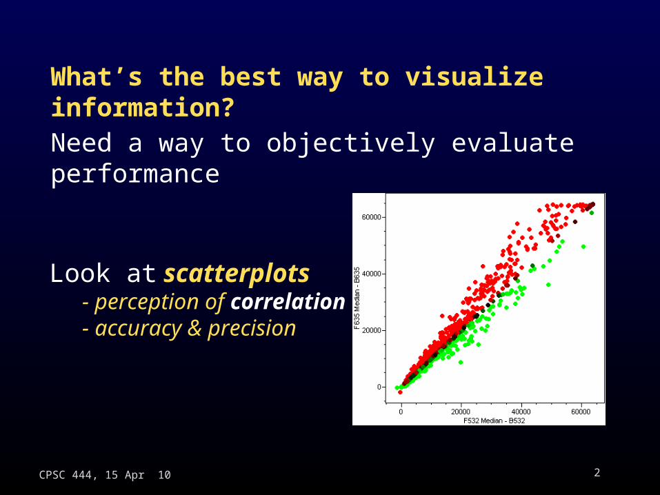
What’s the best way to visualize information?

Look at scatterplots - perception of correlation- accuracy & precision

Need a way to objectively evaluate performance

3CPSC 444, 15 Apr 10

Approach: Use techniques from vision science - decades of experience

- basis of modern theories of perception

Vision Science: Threshold Techniques

E.g., Relation between intensity and brightness

Adjust intensity of test until its brightness just begins to differ from the standard…

One light at fixed intensity (standard)Second light (test) at a different intensity

Light 1 Light 2

Intensity = 10 W Intensity = 10 W

Light 1 Light 2

Intensity = 10 W Intensity = 11 W

Light 1 Light 2

Intensity = 10 W Intensity = 12 W

Light 1 Light 2

Intensity = 10 W Intensity = 13 W

Standard Test

Just noticeable difference (jnd) - 75% correct1 W above standard

A bit more rigorously…

Forced-choice Technique

Q: Which one has the greater intensity?

Look at how accuracy of response varies with difference between test and standard

Intensity = 10 W Intensity = 15 WIntensity = 13 W Intensity = 10 WIntensity = 11 W Intensity = 10 W

Psychometric function

-describes accuracy (probability of correct)as a function of intensity of test light

.

50%

100%

Intensit y of test light

Standard = 10W

10 11 12 13

.

50%

100%

Intensit y of test light

Standard = 10W

10 11 12 13

75%

Threshold (75%) = 10.8 W

.

50%

100%

Intensit y of test light

Standard = 10W

10 11 12 13

75%

Threshold (75%) = 10.8 W

jnd = Δ = 0.8 I W

For I = 10 W, jnd ΔI = 0.8W

For a large range of intensities,

ΔI / I = k = constant

Weber’s Law

For I = 30 W, jnd ΔI = 2.5W

For I = 50 W, jnd ΔI = 4.0W

ΔI / I = .08

ΔI / I = .08

ΔI / I = .08

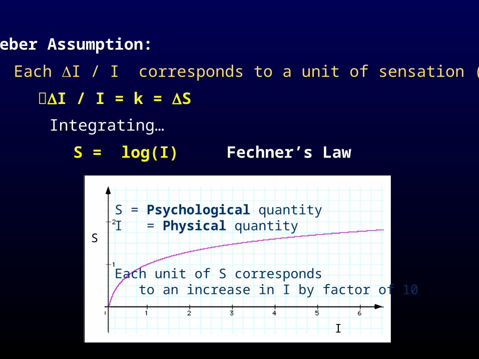
Weber Assumption:

Each ΔI / I corresponds to a unit of sensation (ΔS)

ΔI / I = k = ΔS

Integrating…

S = log(I) Fechner’s Law

S

I

S = Psychological quantityI = Physical quantity

Each unit of S corresponds to an increase in I by factor of 10

9CPSC 444, 15 Apr 10

Approach: Apply this technique to correlation

Forced-choice: Which one has the higher correlation ?

10CPSC 444, 15 Apr 10

1. Fix a particular base correlation (e.g., r = 0.6)

2. Find the jnd Δr (75% correct level) for that correlation- keep showing pairs of scatterplots to observer- adjust differences until jnd is reached- criterion: level in three subwindows is the same

Experimental Procedure - Precision

11CPSC 444, 15 Apr 10

Results.

1.00.50

base correlation (rA)

0.2

0.1

0

from above

from below

Δr = k(1/b - r)

k: variability (= 0.24)

b: offset (= 0.907)

Δu = ku

Δu u

= k

Weber’s Law(with u = 1/b - r)

Only 2 parameters (k,b)to specify precision over all correlations

12CPSC 444, 15 Apr 10

Weber Assumption:

Each ΔI / I corresponds to a unit of sensation (ΔS)

ΔI / I = k = ΔS

Integrating…

S = log(I) Fechner’s Law

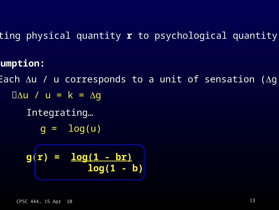
Relating physical quantity I to psychological quantity S

13CPSC 444, 15 Apr 10

Assumption:

Each Δu / u corresponds to a unit of sensation (Δg)

Δu / u = k = Δg

Integrating…

g = log(u)

Relating physical quantity r to psychological quantity g

g(r) = log(1 - br) log(1 - b)

14CPSC 444, 15 Apr 10

Adjust test plot to be midway between reference plots

Experimental Procedure - Accuracy

Start with 0.0 & 1.0. Then 0.0 & 0.5 and 0.5 & 1.0. Then 0.0 & 0.25 and 0.25 & 0.5, etc, etc.

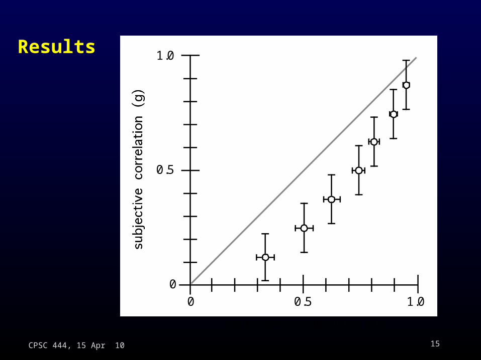
15CPSC 444, 15 Apr 10

Results

.

1.00.50

1.0

0.5

0

objective correlation (r)

16CPSC 444, 15 Apr 10

Results

.

1.00.50

1.0

0.5

0

objective correlation (r)

g(r) = log(1 - br) log(1 - b)(b = 0.9)

Fechner’s law(with u = 1-br)

17CPSC 444, 15 Apr 10

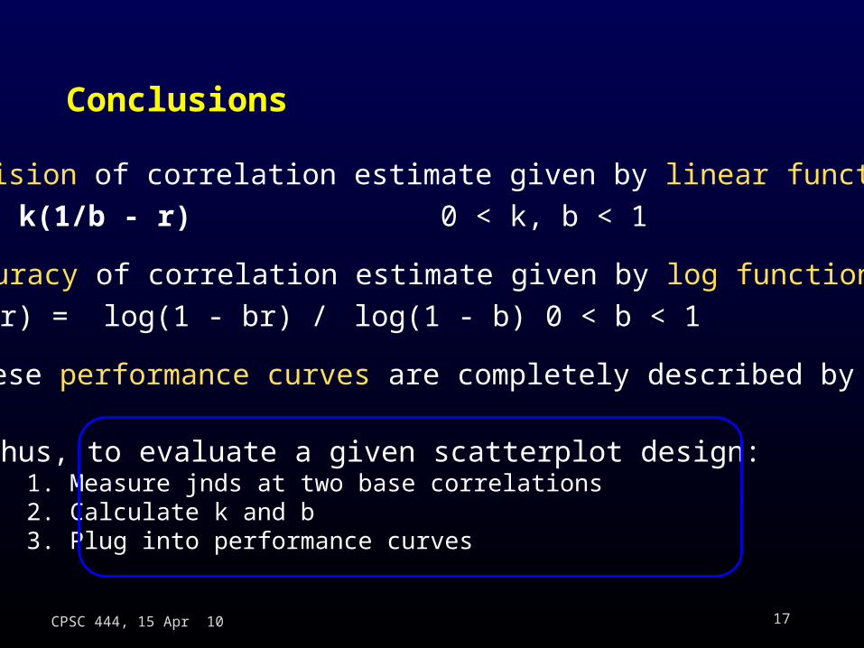
Conclusions

Precision of correlation estimate given by linear function

Δr = k(1/b - r) 0 < k, b < 1

Accuracy of correlation estimate given by log function

g(r) = log(1 - br) / log(1 - b) 0 < b < 1

These performance curves are completely described by k, b

Thus, to evaluate a given scatterplot design:1. Measure jnds at two base correlations2. Calculate k and b3. Plug into performance curves