The People in Your Neighborhood:

Social Interactions and Mutual Fund Portfolio Choice∗

Veronika K. Pool, Noah Stoffman, and Scott E. Yonker†

October 6, 2012

Abstract

We find that socially connected fund managers have more similar holdings and trades. Theportfolio overlap of funds whose managers reside in the same neighborhood is considerably higherthan that of funds whose managers live in the same city but in different neighborhoods. Theseeffects are larger when managers are neighbors longer or are of a similar ethnic background,and are not explained by preferences. Valuable information is transmitted through these peernetworks: a long-short strategy composed of stocks purchased minus sold by neighboring managersdelivers positive risk-adjusted returns. Unlike prior empirical work, our tests disentangle socialinteraction from community effects.

∗We thank Kenneth Ahern, Matt Billett, Martijn Cremers and Ryan Israelsen as well as seminar participants atthe Early Career Women in Finance Conference, the IU-Notre Dame-Purdue Summer Symposium, the University ofToledo, and brown bags at The Ohio State University and Indiana University for helpful comments.†The authors are at Kelley School of Business, Indiana University. Pool: vkpool@indiana.edu; Stoffman:

nstoffma@indiana.edu. Address correspondence to Scott Yonker, (812) 855-2694; syonker@indiana.edu.

Despite the important role professional money managers play in financial markets, and decades

of academic study, relatively little is known about how they generate investment ideas. Research

has found that managers invest in companies headquartered nearby (Coval and Moskowitz, 1999,

2001), and in companies to which they are linked through school networks (Cohen, Frazzini, and

Malloy, 2009). They also choose stocks based on their political ideology (Hong and Kostovetsky,

2012) and stocks with which they are merely familiar (Pool, Stoffman, and Yonker, 2012).

But humans are, as Aristotle famously noted, social animals, so perhaps fund managers also

trade stocks that they learn about from other managers. Exploring this channel is important, as a

large theoretical literature suggests that the social transmission of information by peers can play a

role in determining asset prices.1

While numerous papers examine the effects of social interaction on choices in other domains,2

there is little empirical evidence on how word-of-mouth communications influence professional

investors’ decision to trade a stock. Hong, Kubik, and Stein (2005) take an important first step in

answering this question by studying a broad sample of mutual funds. They show that the holdings

and trades of fund managers who work in the same city are correlated.3 Although these results are

consistent with the hypothesis that professional money managers transmit investment ideas socially,

the authors point out several alternative hypotheses that are difficult to rule out with their data.

Specifically, the correlation in portfolios could be due to fund managers in the same city being

exposed to common local media outlets, being visited by the same corporate executives during

investor-relations road shows, or by geographic segmentation of the job market combined with career

concerns (Scharfstein and Stein, 1990; Chevalier and Ellison, 1999). These alternative “community

effects” would imply that news travels through formal information channels, whereas the social

hypothesis implies that information travels through informal person-to-person relationships.

1Recent theoretical papers include Han and Hirshleifer (2012), Han and Yang (2011), and Colla and Mele (2010).See also the empirical work by Shive (2010), or Hirshleifer and Teoh (2009) for a literature survey.

2For example, Grinblatt, Keloharju, and Ikaheimo (2008) document a substantial influence of near-neighbors onautomobile purchases. Bayer, Ross, and Topa (2008) show the importance of social interaction in labor markets, whileSacerdote (2001) finds strong peer effects on educational outcomes among randomly assigned college roommates.Bertrand, Luttmer, and Mullainathan (2000) find similar effects on welfare participation rates, as do Glaeser, Sacerdote,and Scheinkman (1996) on crime rates.

3Ivkovic and Weisbenner (2007) find similar results for individual investors who live within 50 miles of each other.Feng and Seasholes (2004) show correlated trading among proximate individual investors in China by exploitingbrokerage rules that investors must trade at their branch office. In earlier survey research, Shiller and Pound (1989)found that both individual and institutional investors reported that their portfolio choices were partially driven byinterpersonal communication.

1

Of course, both channels can operate simultaneously, and in this paper we implement a test

that allows us to disentangle the two effects. To identify potential person-to-person relationships,

we use public records data to collect the complete residential address history of fund managers in

our sample, which enables us to determine the pairwise distance between the homes of all managers.

We argue that managers who live near one another (“neighbors”) are likely to come into direct

contact. Managers could meet, for example, at a neighborhood park or school, or while taking the

train to work. We classify managers as neighbors only if they live truly close to each other—for

example, just a fraction of a mile in densely populated areas in Manhattan or Boston (the distance

cutoff varies by population density, as we explain later). Using our distance measure to proxy for

social interaction creates variation within a city that is independent of sharing a media market,

road shows, career concerns-induced herding, or any other community effects.

Thus, while previous papers have documented correlated trading among professional and

individual investors using far coarser definitions of neighbors, we are able to identify the effects

of social contact by zeroing in on fund managers who are likely to know each other, rather than

treating all fund managers based in, say, New York City as neighbors. Prior studies rely on coarse

definitions of neighbors for two reasons. First, they do not have residential addresses for the investors

in their samples. Second, their empirical design tests whether the trades and holdings of investors

are more sensitive to those of nearby investors than to those of a distant cohort. In order to perform

such portfolio-based tests it is necessary to have a sufficient number of nearby investors to form

the nearby cohort for each investor in the sample. As the distance between investors constituting

“nearby” gets smaller, fewer and fewer investors meet this criterion, making such a test impossible to

implement.

We circumvent this problem by designing an empirical test that does not require every investor

in our sample to have a neighbor. We construct measures of pairwise overlap in fund holdings and

trades, and test whether the overlap is greater when fund pairs are managed by neighbors. This

design allows us not only to shrink the distance in the definition of neighbor, but also to control

for the other common community effects that are difficult to separate from the effects of social

interactions in other empirical setups.

Remarkably, the portfolio overlap of funds managed by neighbors is 13% higher in our baseline

model than that of funds whose managers live in the same city but are not neighbors—even after

2

controlling for fund families and investment styles. This increases to 35% when we implement a

cleaner test by focusing on funds with just one manager. We find similarly strong results for trades.

To better identify social networks within neighborhoods, we also collect information on manager

characteristics. Commonality in these characteristics is likely to increase the probability that two

managers interact socially. For example, common ethnic backgrounds could increase the likelihood

of meeting at a church or cultural event, or that their children attend the same school or youth

organization. Our main results are even stronger when managers have the same ethnic background

or have lived near one another longer.

Our results are economically large. The abnormal overlap for neighbors is about the same as it is

for funds that are part of the same fund family, which share analysts. Moreover, the neighbor effects

are about twice as large as the effect of being in the same city (Hong et al., 2005). But despite

the size of the estimates, they are likely to understate the true magnitude of the effects of social

interaction for two reasons. First, while our neighbor measure is a good proxy for whether managers

know one another, it is clearly noisy. If, for example, only half of the managers who we classify as

neighbors actually interact socially, the true effect would be twice the size of our estimates. Second,

managers and other investors have many social networks that we do not capture in the paper.

While shrinking the distance between managers allows us to identify social interaction, it

simultaneously poses another challenge. Since a person’s choice of where to reside is not random, a

manager’s investment decisions may coincide with those of his neighbors because of similarities in

preferences that drive both portfolio and housing choices, rather than personal contact. Indeed, the

economics literature has long recognized the endogeneity problems present when studying social

influence (Evans, Oates, and Schwab, 1992; Manski, 1993).

We conduct several tests to reject this “preferences” alternative. First, our main identification

strategy exploits changes in the residences of managers. If an individual’s preferences are generally

stable through time and similarities in portfolio choices are driven by preferences, then we should see

correlated trading between managers with similar preferences even before they become neighbors.

This is not what we find. Rather, we show that the holdings and trades of managers who are not

neighbors—but become neighbors later in our sample—are not correlated.

3

In another test of the preference story we rely on the observation that managers are limited

in their home choices by the supply of real estate; people can only buy homes that are for sale.

People with overlapping preferences may choose to live in the same residential area, but over small

distances, housing market frictions induce random variation in fund managers’ residential locations.

The distance between managers’ homes is therefore unlikely to decline monotonically with the

closeness of their preferences. In contrast, the social interaction argument suggests that the closer

two people live to one another in a given area, the more likely it is that they will meet. Our results

show that distance matters even within very small areas: overlaps in portfolio holdings and trades

are much higher when managers live within one (population-adjusted) mile than when they live

between one and five miles apart.

In contrast to Hong et al. (2005), we also perform a direct test of whether social influence among

professional investors represents the transmission of valuable information, or if managers are merely

sharing personal sentiments and biases with each other. We address this question by investigating

the performance of overlapping stocks held and traded by neighbors.

We divide each fund’s portfolio into holdings that overlap with those of a neighbor and the

remainder. We then examine whether subsequent performance is better in holdings that are shared

with neighbors. Similarly, we evaluate the performance of a strategy of buying stocks that represent

simultaneous buy trades of the managers and their neighbors and selling short the portfolio of

stocks that neighbor managers sell together. These tests indicate that social interactions create

valuable information transfers between fund managers. In particular, while the sub-portfolio of

holdings that are shared across the neighbors does not outperform the other holdings of the fund,

the long-short strategy of neighbor trades yields a statistically significantly positive abnormal return

of approximately 6% per year. When we exclude the financial crisis, our estimates are around 7%

per year. Our results are similar in magnitude to the estimates reported by Cohen et al. (2008) of

the abnormal returns generated from information shared between executives and fund managers.4

The finding that valuable information appears to be shared casts additional doubt on the preferences

alternative.

4Cohen et al. (2008) show that information shared in these networks generates abnormal returns of 7.8% per year.Our focus is on information transmission in networks of peers, rather than between managers and informed insiders.While it is certainly important to know if fund managers exploit their links to inside information, the question ofwhether valuable information is shared between professional investors has remained unanswered.

4

The social transmission of value-relevant information is particularly interesting in our setting

given that the sharing is among potential competitors. There are several possible explanations for

this phenomenon. First, since we don’t observe trading behavior within the quarter, it is possible

that managers who have bought a stock subsequently share their information in an effort to have

information impounded in prices more quickly. Similarly, managers may also openly announce their

information to induce coordinated trading among their peers in order to mitigate synchronization

risk (Brunnermeir and Abreu, 2002). Second, the cost of sharing information is not likely to be high;

the effect on relative performance of sharing a few stock picks is probably small. Third, managers

may have an expectation of quid pro quo, so sharing information now could help them in the future.

Stein (2008) discusses some of these possibilities and provides a model of information exchange

consistent with what we document here.

1 Data and sample construction

We combine several data sources in this study. First, we draw information on fund managers

from Morningstar, which reports the name of each manager for a fund (including individuals on

team-managed funds), their start and end dates with the fund, and information about the manager’s

educational background. We limit the sample to actively-managed U.S. equity funds by filtering

Morningstar style categories and manually screening fund names.

We obtain mutual fund holdings from the Thomson Financial CDA/Spectrum Mutual Fund

database, which contains the quarter-end holdings reported by U.S.-based mutual funds in mandatory

SEC filings. Thomson uses two date variables, RDATE and FDATE, which refer to the actual

date for which the holdings are valid and the Thomson vintage date on which the data were cut,

respectively. We follow standard practice and restrict the holdings to those observations where the

FDATE is equal to the RDATE to avoid the use of stale data in our analysis. We drop observations

when the stock price, CUSIP, or the number of shares held are missing. From this starting point,

there are 4,685,084 quarterly fund-holding observations from the first quarter of 1996 to the fourth

quarter of 2010. The sample includes 2558 funds and 4622 managers, with an average of 810 funds

per quarter.

5

To focus on funds for which we can properly control for fund style, we restrict the sample to

those funds with a Morningstar category in the 3-by-3 size/value grid (US Large Blend, US Large

Growth, US Large Value, US Mid-Cap Blend, US Mid-Cap Growth, US Mid-Cap Value, US Small

Blend, US Small Growth, or US Small Value). We also remove funds with fewer than 20 holdings,

or more than 500. Funds with more than 500 holdings could be index funds that were missed in our

first set of screens. Adding these screens reduces the sample to an average of 688 funds per quarter.

1.1 Pairwise distances

Our goal is to identify pairs of managers who have homes close to each other. We follow the method

of Yonker (2010) and Pool et al. (2012) to identify fund managers in the LexisNexis Public Records

database using name, age, and location searches.5 These data include a history of all addresses

associated with each person, including all owned or rented properties. The data are extensive,

drawing on public records from county tax assessor records, state motor vehicle registrations, reports

from credit agencies, court filings, and post office records, among other sources. We are able to

identify 2042 managers in the database of the 4622 managers in the initial sample. Our final sample

includes 422 funds, or an average of just over 70,000 fund-pairs per quarter. The sample coverage

is very similar to Pool et al. (2012), who show that their sample is representative of the broader

sample of actively-managed mutual funds, covering over 80 percent of actively managed mutual

funds by assets under management.

Whenever possible, we identify the addresses (including vacation homes) of each manager at

the beginning of each quarter. We then calculate distances between each pair of managers using

the latitude and longitude of the centroid of each home’s zipcode.6 We refer to this distance as

zipdistance. To get more precise travel distances for nearby pairs, we next determine the driving

distance between any two managers where zipdistance ≤ 5 miles. This includes all pairs of managers

5See Pool et al. (2012) for a detailed explanation of the matching procedure.6The distance in miles between two points with latitude/longitude pair (φi, λi) is calculated using the Vincenty

formula for distances on ellipsoids,

distance = 3963.19 × arctan

√

(cosφ2 sin ∆λ)2 + (cosφ1 sinφ2 − sinφ1 cosφ2 cos ∆λ)2

sinφ1 sinφ2 + cosφ1 cosφ2 cos ∆λ

,

where ∆λ = λ2 − λ1. This formula is known to work well for both short and long distances.

6

who live in the same zip code, as zipdistance = 0 for these pairs. We identify 281,605 such pairs,

and for each one we use an online driving directions tool to record the precise travel distance between

the two addresses.7 For managers with more than one home, we record the minimum pairwise

distance as the unique distance for the pair.

We make one further refinement to our distance measure. Two managers who live one mile apart

in Manhattan are clearly further from each other in terms of “social distance” than two managers

who live one mile apart in the considerably less-populated town of New Canaan, CT, where several

managers live. With more than 30,000 people per square mile in Manhattan, the probability of

two people knowing each other is clearly much lower. We therefore calculate a normalized distance

measure that accounts for the population density of the area where managers live. For each zip

code, we calculate the “household density” by dividing the number of households by the land area

of the zip code.8 The normalized driving distance between manager i and j is then calculated as

NDDi,j = Driving distancei,j ×max(hhdensi, hhdensj)

median(hhdens),

where hhdensi denotes the household density of manager i’s zip code. The median density, calculated

across all observations in the sample, is 903.8 households per square mile. The calculation implies

that one normalized mile is just 60 feet on the Upper East Side of Manhattan, while in New Canaan

it is 2.9 miles. It is approximately one mile in the Boston suburb of Wellesley, or in Colorado

Springs, CO.

1.2 Neighbors

Our main variable of interest will be an indicator variable for whether two fund managers are

“neighbors.” Therefore, we must specify some threshold distance below which we will classify

managers as neighbors. We do this by first creating another dummy variable, DistBtwnHms1Mile,

7We only calculate driving distance for potentially close pairs because the precision of the distance measure mattersmore for short distances: since we will classify managers as “neighbors” or not, it matters much more if two managersare really within one mile of each other than if they are within 100 or 101 miles of each other. It is also not feasible touse online tools to determine driving distances for tens of millions of pairs. To avoid problems with one-way streetscausing artificially long distances when calculated as driving distances, we collect walking distances for the five biggestcities in our sample, and confirm that our results remain qualitatively unchanged.

8Figures for population and land area are obtained for zip code tabulation areas from the 2000 census.

7

that takes a value of one when managers live within one (non-normalized) mile of each other. As

shown in Table 1, this condition is true in 0.37% of our observations.

We then choose a threshold for the normalized distance measure, NDD, that has exactly the

same mean. This threshold turns out to be 2.9 normalized miles, so we set the Neighbors dummy

to take a value of one if two managers live within 2.9 normalized miles of each other. Continuing

the example from earlier, for managers who live on the Upper East Side to be considered neighbors

they must live in the same or adjacent building (within 175 feet), but managers in New Canaan can

live up to 8.4 miles apart.

The neighbor cutoff is of course somewhat arbitrary, but robustness tests confirm that our

results are not sensitive to this particular distance. In general, requiring neighbors to live even closer

causes our coefficient estimates to increase, but the standard errors increase as fewer people are

included in the neighbor category. While the same number of managers are classified as neighbors

by the DistBtwnHms1Mile and Neighbor dummies, different managers are classified as neighbors

under each measure—the Neighbor dummy includes more managers from less-populated areas,

where the probability of knowing each other is higher. As we show in the next section, it turns out

that the Neighbor dummy has considerably more power to detect portfolio correlations than the

DistBtwnHms1Mile variable.

1.3 City clusters

We group fund managers into cities based on the location of their residences. We begin with the

location of the centroid of each manager’s zip code, and then group zip codes into cities using an

agglomerative hierarchical clustering algorithm.9 Each zip code begins as its own cluster, and zip

codes—and then clusters—are grouped iteratively using the average linkage method until all clusters

are at least 50 miles apart. For example, the clustering method creates a New York City cluster

that includes Manhattan and the other boroughs, as well as communities in eastern New Jersey.

Bedroom communities in upstate New York such as Scarsdale and Rye are grouped with other

towns in Connecticut to form another cluster.

9We do this rather than using the name of the city in which a zip code is situated because we want to includesuburbs in each city grouping.

8

The locations of these cities are shown in Figure 1. The circles are centered at the weighted-

average location of all zip codes in the cluster, where the weight is the number of unique managers

with a home in each zip code. The size of the circle shows how many unique managers have a

residence in each city during our sample period. The proportion of these managers who are part

of a neighbor pair at some point during the period is shown as a shaded pie slice. It is clear from

the picture that managers are widely disbursed, and that while pairs are more likely to be found

in larger cities, they are also quite disbursed. Cities with only one fund manager do not have any

neighbor pairs, but we include these managers in our sample to provide information about typical

holdings and trades.

2 Do social interactions influence fund holdings and trades?

We begin our empirical analysis by testing whether social interactions influence the holdings and

trades of mutual funds. We do so by creating portfolio overlap measures in holdings and in trades

between fund pairs and testing whether these measures are greater for fund pairs with managers

who are neighbors. This pairwise methodology creates a large number of observations since the

number of unique pairs of N funds is N(N − 1)/2. Given the pairwise structure of the data, we

are careful to calculate standard errors in a way that allows repeated observations of a firm to be

correlated. In particular, our observations are not independent since we calculate N − 1 overlaps for

each fund in each quarter. A common component in each of these observations is the portfolio of

that fund. Moreover, fund portfolios are persistent over time. While this correlation does not bias

the coefficient estimates, it will underestimate the standard errors. We therefore report standard

errors that have been two-way clustered by each fund in the fund pair.

The average number of funds in the sample each quarter is 422 and our analysis includes 60

quarters, so we should have over 5.3 million quarterly fund-pair observations. However, since

mutual funds are constrained by their investment mandates, it is difficult for funds in different

size categories to engage in overlapping trades. Specifically, large-cap funds are constrained from

trading in small-cap stocks and vice versa. For this reason we exclude pairs where one member is a

large-cap fund and the other is a small-cap fund. This reduces the sample to approximately 4.2

9

million quarterly observations. Notably for the standard errors, however, the number of funds used

in the clustering calculation is 1699.

2.1 Social interactions and holdings

We first investigate whether the overlap in holdings is greater for funds whose managers are neighbors.

We measure the portfolio overlap in holdings between funds i and j during quarter t as:

PortOverlapi,j,t =∑k∈Ht

min{wi,k,t, wj,k,t}, (1)

where wi,k,t is fund i’s portfolio weight in stock k during quarter t, and Ht is the set of all stocks

held by funds i and j during t. We aggregate the overlap measure to the fund level since conducting

the analysis at the stock level would lead to well over a billion observations.

Using this measure of overlap, we estimate the regression

PortOverlapi,j,t = βNeighborsi,j,t + δSameMFCityi,j,t

+ γSameMediaMkti,j,t + Γ′Controlsi,j,t + εi,j,t, (2)

where Neighborsi,j,t is a dummy variable that is one if at least one manager from fund i is a

neighbor (as defined in Section 1.1.2) of a manager from fund j during quarter t, SameMFCityi,j,t

is a dummy variable that is one if funds i and j are headquartered in the same city (defined as in

Section 1.1.3 but using mutual fund company addresses), SameMediaMkti,j,t is a dummy variable

that is one if at least one pair of managers for a given fund pair live within 50 miles of one another,

and Controlsi,s,t is a vector of relevant control variables.

We include the following controls: dummy variables that are one if funds i and j match

on Morningstar size or value/growth categories (BothSmallCap, BothMidCap, BothLargeCap,

BothV alue, BothGrowth, BothBlend), the absolute value of the difference between the total net

asset-based quintiles of funds i and j (TNAQuinDiff), the average TNA-based quintiles of funds

i and j (TNAQuinAvg), and dummy variables that indicate if funds i and j are from the same

mutual fund family (SameFundFam), at least one pair of managers from funds i and j manage

10

at least one other fund together (MngOtherFundTogether), and funds i and j have at least one

manager in common (CommonMgr). In most of the subsequent analyses we exclude observations

where funds have a common manager, but it is interesting to include these observations in our initial

regressions so we can compare the magnitude of the effect of being neighbors to that of having a

manager in common.

If social interactions influence mutual fund managers’ portfolio choices, then β in equation (2)

should be should be positive. The estimate of β is the incremental increase in portfolio overlap

from managers being residential neighbors beyond the influence of local media and what Hong et al.

(2005) call “local investor relations.” The effect of managers being exposed to the same local media

is captured by SameMediaMkt and any influence of the relative proximity of the mutual funds

themselves, such as local investor relations, is captured by SameMFCity.

Table 1 reports the means and standard deviations of the variables used in the analysis. The

table shows that the average portfolio overlap between two funds in the sample is 8.03% and that

0.37% of fund pairs have at least one manager pair that are neighbors. While this may appear to be

a small number of neighbors, about 44% of funds in each quarter have at least one manager who is

a neighbor of a manager at another fund, so the results are not driven by just a few funds. The

table also shows that 10.46% of fund pairs have at least one manager pair that lives within 50 miles

of one another, 7.12% of fund pairs are located in the same city, and 2.62% of fund pairs are from

the same family. There is also a great deal of variation in our dependent variable, the standard

deviation of PortOverlap is 9.43%.

Table 2 displays the coefficient estimates and standard errors for various forms of equation (2).

Standard errors are two-way clustered at each fund’s level in the fund pair. In column 1 we include

only SameMFCity and the control variables. This regression gives us an estimate of the magnitude

of the Hong et al. (2005) results in our empirical framework. The coefficient on SameMFCity is

65 basis points (bps) and is significantly greater than zero. Given the average overlap in holdings

in the sample of 8.03%, this implies that the portfolio overlap of funds located in the same city is

about 8% greater than funds located elsewhere.

The estimates on the control variables are also of interest. Not surprisingly, matching on fund

size and value/growth categories is extremely important for explaining the commonality in holdings

11

of two mutual funds, with large-cap fund pairs having the greatest portfolio overlap. Among the

other fund linkages included in the controls, having a manager in common has the largest effect.

The portfolio overlap increases by 10.42% in this case, implying that for the average fund pair the

portfolio overlap is over 125% higher if they have a manager in common. When two funds have

managers who manage a third fund together, the portfolio overlap is also higher. The estimate

on MngOtherFundTogether is 211 bps, implying that the overlap between these funds is about

26% greater. Finally, funds that belong to the same fund family also have higher overlaps. This

abnormal commonality in holdings is 103 bps and may be due to common research departments or

work-related interactions.

In column 2 we add a measure that captures whether the fund managers are neighbors based

on raw driving distance. For a given fund pair, the variable DistBtwnHms1Mile is a dummy

variable that takes the value of one if at least one of the managers of a fund lives within a one-mile

driving distance from one of the managers of the other fund, and is zero otherwise. The estimate on

DistBtwnHms1Mile is 88 bps and statistically significant. This indicates that when we compare

two fund pairs that are located in the same city—one with managers who live within a mile of

one another and the other with managers who do not—the fund pair whose managers also share a

neighborhood will have 88 bps higher overlap. Since the magnitude of SameMFCity is 64 bps, if a

pair of funds have managers who live within a mile of one another and the funds are located in the

same city, then their portfolio overlap will be 64 + 88 = 152 bps greater than that of fund pairs

from different cities.

As discussed earlier, one problem with using raw driving distance to measure social interactions

is that distance alone does not capture the probability that two individuals actually know one

another. As we describe in Section 1, we therefore scale driving distances between managers to

adjust for the household density of the managers’ residential areas. This increases the “social

distance” in more densely-populated areas and shrinks it in less densely-populated regions. We then

choose a cutoff for our variable of interest, Neighbors, so that it is true for the same number of

managers as those that live one mile apart.

In column 3 we replace DistBtwnHms1Mile with Neighbors. It is apparent that we are

choosing neighbors much more appropriately using the normalized driving distance measure. The

coefficient estimate on Neighbors is 134 bps, 1.5 times that on DistBtwnHms1Mile.

12

In column 4 we add SameMediaMkt to control for managers living within 50 miles of one

another. Even if funds are located in different cities, it is possible that managers live close to each

other. They could vacation in the same area or they may manage their funds remotely, spending

most of their time away from the fund headquarters. SameMediaMkt takes these possibilities into

account and should also capture broad local effects, such as managers being exposed to common

media sources. The estimate on SameMediaMkt is 38 bps and is statistically significant. Its

inclusion in the regression reduces the magnitudes of both SameMFCity and Neighbors, but of

the three, the magnitude of Neighbors is still the largest at 105 bps.

We come to our “baseline” regression in column 5, where we exclude fund pairs with common

managers. In this specification the estimates on Neighbors, SameMFCity, and SameMediaMkt

are 108 bps, 49 bps, and 38 bps, respectively. This implies that two funds that are located within

the same city with at least one pair of managers who are neighbors will have 195 bps greater overlap

than the typical fund pair. This is equivalent to over 195/803 = 24% greater commonality in

holdings. The coefficient estimates decompose this effect into social interactions and broad local

effects, the former representing over half of the total magnitude.

To put the influence of having fund managers who are neighbors in perspective, we can compare

the coefficient estimates on Neighbors to that on some of the other control variables. For instance,

two funds from different families located in the same city with managers who are neighbors will

have a comparable overlap in holdings to two funds in the same fund family. Additionally, the

effect on fund holdings from social interactions is 57% of the effect of two funds having managers

who manage another fund together. Of course, we cannot be sure that all neighbors in our sample

actually know one another. If only half the managers that are identified as neighbors actually know

one another, and we were instead able to estimate the regression with only the managers who do

know one another, then we would expect the coefficient estimate to be twice as large, which would

be quite similar to the overlap in funds whose managers manage another fund together.

The regression in column 6 excludes all fund pairs within the same fund family. Not surprisingly,

the coefficient estimates on Neighbors and the two local effects measures decrease, but they remain

significantly positively estimated and economically relevant. The results confirm that even across

families, fund managers are willing to share information about their holdings.

13

Finally in column 7, we estimate equation (2) for the sample of fund pairs that only include

funds managed by just one manager (“single”). Since both funds in these fund pairs have managers

who are sole decision-makers, we would expect that when these managers are neighbors, social

interactions will be more important. We find that this is the case. The coefficient estimate on

Neighbors is 280 bps, statistically significant at the better than 1% level. The estimate suggests

that the effect of social contact on portfolio overlap is remarkably large; it leads to 35% greater

overlap than that of the the average fund pair in the sample.

2.2 Social interactions and trades

We next investigate whether fund pairs managed by neighbors are more likely to make similar trades

than those that are managed by non-neighbors. In order to do so we construct measures of overlap

in both purchases and sales. We measure overlap in stock purchases and sales as:

BuyOverlapi,j,t =

∑k∈Tt min{I+

i,k,t, I+j,k,t}

min{∑

k∈Tt I+i,k,t,

∑k∈Tt I

+j,k,t}

, (3)

SaleOverlapi,j,t =

∑k∈Tt min{I−i,k,t, I

−j,k,t}

min{∑

k∈Tt I−i,k,t,

∑k∈Tt I

−j,k,t}

, (4)

where I+i,k,t is one if fund i increased the number of shares in stock k between time t − 1 and t,

and is zero otherwise, I−i,k,t is one if fund i decreased the number of shares in stock k between time

t− 1 and t, and is zero otherwise, and Tt is the union of all stocks traded by funds i and j. The

numerators of these measures simply report the number of common buys and sales, respectively, of

the funds in a fund pair. These numbers are then normalized by the minimum number of buys and

sales, respectively, of the two individual funds, so the measures range from zero to one.

To see how these measures work, suppose that fund i makes 100 trades during quarter t and that

40 trades are buys and 60 are sales. During the same quarter fund j executes 50 trades, 30 of which

are buys and 20 are sales. Assume further that funds i and j buy 10 stocks in common and sell 5

stocks in common. In this case BuyOverlapi,j,t = 10/30 = 33% and SaleOverlapi,j,t = 5/20 = 25%.

14

In Table 3 we test whether social interactions affect the trading behavior of mutual fund

managers by estimating regression equation (2) using the purchase and sale overlap measures defined

in equations (3) and (4), respectively, as the dependent variables. We estimate the regressions using

four different specifications for both purchases and sales: the full sample of fund pairs, the sample

excluding fund pairs with common managers, the sample excluding fund pairs within the same fund

family, and fund pairs managed by single managers. The results are similar to those of Table 2;

fund pairs that have managers who are neighbors have significantly more overlap in trades than

those that do not.

For common buy trades, the baseline model (column 2) indicates that fund pairs with managers

who are neighbors have 119 bps more purchase overlaps than those that live within 50 miles of one

another. Given that the average purchase overlap is 851 bps between fund pairs, this suggests that

funds with managers who are neighbors have 14% greater commonality in trades than do funds

whose managers live within 50 miles of one another. The most striking results are for the sample of

single manager pairs. The coefficient estimate on Neighbors is 481 bps, suggesting that the impact

of social interactions on single managed funds is huge; fund pairs with single managers who are

neighbors have over 50% higher overlap in their buys than the average mutual fund pair in the

sample.

The magnitude of the impact of social interactions for stock sales is smaller, although the

Neighbors estimate of 63 bps in the baseline model (column 6) is statistically significant at the 5%

level. This asymmetry is not surprising because mutual funds face short sale constraints so overlap

in sales is conditional on both funds in a pair already owning the stock. Moreover, these short

sale constraints lead to an asymmetry in how managers respond to information. For example, if a

manager receives a positive signal about a stock, she can respond by either expanding the position

if she already owns the stock (an “intensive margin buy”), or by establishing a new position if she

does not (an “extensive margin buy”). Both actions can be arbitrarily scaled—subject to regulatory

limits—and reveal an equally strong conviction. But if the signal is negative, the strongest response

is to liquidate the position (“extensive margin sell”). Therefore, on the sell side, we would expect

that social interactions are more likely to induce extensive margin transactions, but on the buy side

we would expect no such asymmetry.

15

To examine this, we decompose purchases and sales into extensive and intensive margins. We

use an approach analogous to that in equations (3) and (4) to calculate these alternative overlap

measures. By construction, for each fund pair and for both buys and sales, the sum of the intensive

margin overlap and the extensive margin overlap that requires at least one of the funds to trade

on extensive margin is equal to our original overlap value. The results are summarized in Table 4.

The table confirms that for buys, both extensive margin and the intensive margin overlap measures

are statistically significant, but for sales the Neighbors coefficient is significantly positive only for

extensive margins.

2.3 Social interactions vs. preferences

Although our empirical methodology can disentangle the role of social interactions in portfolio choice

from that of local effects, such as media and local investor relations, a potential concern about

our Neighbors variable is that it may be measuring similarities in manager preferences and not

the likelihood of social contact. This means that the correlation we uncover between our portfolio

overlap measures and the Neighbors indicator may be driven by unobserved characteristics of these

managers, rather than by network effects. Indeed, managers choosing the same residential areas

may be similar on many dimensions including wealth, age, political affiliation, and ethnicity. There

is empirical evidence that political values, for example, affect the portfolio choices of mutual fund

managers (Hong and Kostovetsky, 2012). In this section we address this alternative explanation.

Our first test of the “preference explanation” exploits residential relocations of managers. If

managers with similar preferences tend to select into similar neighborhoods and these common

preferences are driving the commonality in trades and holdings, then these managers should

exhibit similar trading behavior prior to becoming neighbors.10 To test this, we create two

additional variables, FutureNeighbors and PastNeighbors. FutureNeighborsk,l,t is a dummy

variable that is one if managers k and l are neighbors for some s > t but are not neighbors for

10Our test relies on the traditional economic assumption that preferences over investment behavior are stable throughtime. Recent empirical evidence supports this view: Barnea, Cronqvist, and Siegel (2010) show that about one-thirdof investment behavior is determined by genetics alone. Cesarini, Dawes, Johannesson, Lichtenstein, and Wallace(2009) and Cesarini, Johannesson, Lichtenstein, Sandewall, and Wallace (2010) find similar results for risk-taking. Seealso Andersen, Harrison, Lau, and Rutstrom (2008).

16

s ≤ t. PastNeighborsk,l,t is a dummy variable that is one if managers k and l are neighbors for

some s < t, but are not neighbors for s ≥ t.

We add these variables to the regression in equation (2) with one change. Instead of using

fund-pair observations we use manager-pair observations. We do this because relocations are

unique to managers and not funds. We also use this specification later when investigating how the

demographics of neighborhoods and characteristics of managers affect our variables of interest. As a

result we now have multiple observations for fund pairs with more than one manager. This means

that the observations are not independent, so we continue to two-way cluster the standard errors by

each fund in the pair. As we will show later, our estimates and standard errors using the manager

-pair specification are nearly identical to those in the collapsed fund-pair specification.

In Table 5 we report estimates of

Overlapi,j,t = βfFutureNeighborsk,l,t + βNeighborsk,l,t + βpPastNeighborsk,l,t

+ δSameMFCityi,j,t + γSameMediaMktk,l,t + Γ′Controlsi,j,t + εi,j,t, (5)

where Overlapi,j,t is the holding or trade overlap between funds i and j at time t, and manager k is

a manager of fund i, while manager l is a manager of fund j. Note that the Neighbors variable is

also manager-specific in this specification.

If overlapping preferences drive the commonality in trades and holdings between neighboring

managers, then the estimate of βf should be positive and significant. The table shows that this is

not the case. The coefficient estimates on FutureNeighbors for overlap in holdings, purchases, and

sales are not statistically different from zero. The coefficient estimates on Neighbors are significantly

estimated at 113 bps, 111 bps, and 56 bps for overlap in holdings, purchases, and sales, respectively.

Interestingly, there is some evidence that past neighbors may remain in contact and continue to

discuss investment ideas. The coefficient estimate on PastNeighbors is positive and significantly

estimated for overlap in holdings and is positive, but not statistically different from zero, for overlap

in both purchases and sales.

As a second test of the preference story, we include additional demographic control variables in

our quarterly manager-pair specification. If managers select certain neighborhoods that match their

17

preferences, then controlling for the characteristics of those neighborhoods should eliminate or at

least reduce the effect of preferences on investment behavior. Unlike our distance measures, these

demographic control variables allow us to test whether managers living in similar environments in

different parts of the country exhibit similar investment behavior. For instance the demographic

control variables will pick up whether a manager who lives in a highly religious area of Ohio is likely

to invest similarly to a peer who lives in highly religious area of California.

Specifically, we control for the effects of common religious beliefs and similar wealth by including

five additional variables in our regression specifications. BothReligiousAreas, BothJewishAreas,

andBothCatholicAreas are dummy variables that are one if the percentage of the population that are

religious adherents, adherents to Judaism, or adherents to Catholicism in both managers’ counties of

residence are greater than the 75th percentile in the sample, respectively. BothHighHmV alueAreas

(BothLowHmV alueAreas) is a dummy variable that is one if the median home price in both

managers’ zip code of residence is greater than the 75th percentile (less than the 25th percentile) in

the sample.11

For each measure of overlap, Table 6 reports the results from the baseline regression and the

regression including the additional demographic control variables using our quarterly manager-pairs

specification. While the religious control variables are highly significant in all specifications, they

do not significantly alter the coefficient estimates on Neighbors. Including these control variables,

however, does substantially reduce the coefficient estimates of SameMediaMkt for all three overlap

measures. For instance, when investigating the overlap in holdings between funds, the estimate on

SameMediaMkt falls from 52 bps to 11 bps after including the demographic control variables and

for purchase overlap the coefficient estimate falls from 76 bps to 33 bps.

Our final test of the preference story is based on the idea that managers are not perfectly mobile

in their home choices. Preferences may drive a manager to live in a certain suburb or area of a city.

The manager may even find the perfect home that matches his preferences, but if the home is not

for sale he must choose another home. Therefore, people with the most similar preferences will live

within a small area, but within that area they will be allocated based on the supply of real estate at

the time they moved to the area. The social interaction story however suggests that the closer two

11County-level religious data are from the U.S. Church Membership Data from the Association of Religious DataArchives (www.thearda.com). Zip code-level median home prices are from the 2000 census.

18

people live to one another, the more likely it is that they will have social contact, and this is true

even within very small areas.

We therefore estimate our baseline regression, but add dummy variables that indicate if funds

have managers who live within one normalized mile, one to five normalized miles, five to 10 miles,

10 to 25 miles, and 25 to 50 miles. The results are displayed in Figure 2. The figure shows that

overlap in holdings and trades is much higher for funds that have managers who live within one

normalized mile of one another than for those with managers who live between one and five miles of

one another. In fact the abnormal overlap in purchases for the sample of single managers is 788 bps

for managers who live within one mile, while it is 220 bps for managers who live between one and

five miles of each another. Thus in order to favor the preference story over the social interaction

story one must believe that the preferences of managers who live within one mile of each other

are over 3.5 times more similar than managers living between one and five miles of one another.

Given the frictions in the real estate market and that mutual fund managers are certainly a more

homogeneous group than the general population, this would be very surprising.

2.4 Manager characteristics

Up to this point, we measure the likelihood of social contact using the distance between two

managers’ homes. However, the likelihood can be further refined within the group of neighbors:

social interactions may be more likely or frequent between those neighbors who share common

characteristics or among neighbors who have known each other longer. The idea that people gravitate

toward those who are similar to themselves, called homophily, is well-established in the sociology

literature (Lazarsfeld and Merton, 1954). Common characteristics between neighbors could proxy

for the quality of their network (Bertrand et al., 2000), so we expect that when the network quality

is higher, the manager pair has a greater commonality in their trades and holdings. We test this

by interacting Neighbor with various manager-specific characteristics. The characteristics that we

investigate include neighbor tenure, age, ethnicity, portfolio management experience, and college

attendance.

Specifically, NeighborsTenure is the number of years two managers have been neighbors,

SimilarAge is a dummy variable that is one if the difference in the managers’ ages is less than

19

the median in the sample (10 years), and SameEthnicity is a dummy that is one if the managers

are of the same minority ethnicity.12 BothExp (BothInexp) is a dummy variable that is one if

both managers have more (less) portfolio management experience than the median manager in the

sample. SameCollege is a dummy variable that is one if both managers attended the same college

or university. For the remainder of the paper we only display the results for holding and purchase

overlaps since sale overlaps convey a similar picture and are less informative because commonality

in sales is conditional upon both funds holdings the stock.

The results of the tests are summarized in Table 7. The results in the first column show that

managers who are neighbors longer have greater overlap in holdings and purchases. For each year

that managers are neighbors, their portfolio (purchase) overlap increases by 19 (25) bps. Not only

is this result intuitive if the Neighbors dummy is capturing the likelihood of social interactions, but

it also casts additional doubt on the preference story since the length of time two managers live

near each other is unlikely to increase the similarity in their preferences.

The analysis in the remaining columns of the table show that funds managed by neighbors who

are more likely to interact socially because of homophily have greater commonality in their holdings

and trades. Fund pairs with managers who are neighbors and are of a similar age have a higher

overlap in both holdings and purchases though the coefficients are not statistically significant. Funds

with managers who are neighbors and are of the same ethnicity have a remarkably high overlap in

holdings and purchases. Their commonality in holdings is 373 bps more than that of funds that are

managed by neighbors who do not have the same minority ethnicity.

The specifications that include interactions with BothExp and BothInexp give us the first

indication in the paper as to what type of information is spread through social interaction. Is

value-relevant information spread through social contact or is it merely irrationally exuberant

information? The table shows that at least one manager in each pair must be experienced in order

for there to be investment related information flow between neighbors. The greatest overlap occurs

in funds where both managers are experienced. In these cases the abnormal holding overlap is

12We use a classification algorithm developed by Ambekar, Ward, Mohammed, Male, and Skiena (2009) to classifynames into one of thirteen categories, including Indian, Jewish, Muslim, East Asian, and others. The classifier appliesa Hidden Markov Model trained with names gathered from Wikipedia. We classify a fund manager as belonging toa group if the predicted probability assigned by the algorithm is above 85%. Visual inspection of the classificationresults confirms that the algorithm appears to perform well.

20

112 bps more than when one manager is experienced and the other is not. For purchases, the

abnormal overlap among neighbors only occurs when both neighbors are experienced portfolio

managers. We return to this issue in the next section.

2.5 Stock characteristics

Having established that social interactions affect the holdings and trades of mutual fund managers,

it is interesting to test whether there are distinct patterns in the types of stocks in which the

influence of social interactions are greatest. Thus we create measures of overlap in holdings and

purchases for subsets of different types of stocks. These overlap measures are created analogously

to the overlap measures in equations (1) and (3). For example, the holdings overlap for S&P 500

stocks is computed as in (1) with the additional condition that k ∈ S, where S is the set of stocks

that are included in the S&P 500 index. Similarly, the holding overlap for non-S&P 500 stocks is

subject to the constraint that k /∈ S. The sum of these overlap measures is then equal to the total

overlap in holdings between funds in the sample. Notice that in Table 8 the average overlap of S&P

500 stocks is 6.75%, while the overlap in non-S&P 500 stocks is 1.22%, the sum of these is roughly

equal to the total holding overlap in the sample of 8.03%.13

In Table 8 we report coefficient estimates and standard errors for Neighbors, SameMediaMkt,

and SameMFCity from the baseline version of equation (2) for overlaps in purchases and holdings

of different types of stocks. We also report the average overlap in the sample for each overlap

measure so that the coefficient estimates can be interpreted on a relative basis. In the first two

rows we report the estimates for local and non-local stocks. Coval and Moskowitz (2001) find that

mutual fund trades in local stocks are informed. Ivkovic and Weisbenner (2007) find that individual

investors are much more sensitive to the trades in local stocks of peers within 50 miles. Since there is

evidence that local investors are informed investors, they interpret this as evidence that information

diffusion effects are informed. We find similar results for mutual fund managers. Mutual fund pairs

managed by managers who live within 50 miles of one another have 25% higher overlap in local

stocks than the average fund pair in the sample (22 bps/88 bps). However, that effect is likely driven

by the influence of the common media sources or local investor relations and not social contact.

13For several of these characteristic overlap measures the sum of the two subsets is smaller than 8.03%. This is dueto data availability of the characteristics.

21

Fund pairs whose managers are neighbors have lower than normal overlaps in local stocks. In fact,

the abnormal overlap in local stocks for fund pairs that are neighbors is essentially zero (−23 bps

+22 bps).

We next investigate whether the portfolio overlap is particularly high in politically sensitive stocks.

Hong and Kostovetsky (2012) find that mutual fund managers who make campaign contributions to

Democratic candidates tend to be “closet socially responsible investors”. If certain neighborhoods

tend to be more “Republican” or more “Democratic” then we might find that the abnormal overlap

tends to manifest itself in either politically sensitive stocks or non-politically sensitive stocks. The

results show that social interactions only influence stocks that are not politically sensitive, however

the politically sensitive stocks are so few in number that the effect of social interactions may be

difficult to detect.

In the next several rows of the table we split stocks based on various measures of visibility and/or

levels of asymmetric information. Finding that social interactions are stronger among “harder to

research stocks” may hint at value-relevant information flowing between managers through this

channel. The relative overlap in S&P 500 stocks and non-S&P 500 stocks is very similar at around

13% for S&P 500 stocks and 16% of non-S&P 500 stocks (for both holding and purchase overlaps).

For stocks split by analyst coverage, the low analyst coverage stocks have much higher relative

abnormal overlap, but again there is so little overlap in low analysts stocks that it is difficult to say

that much of the overall commonality in trades is due to stocks with low analyst coverage.

If irrationally exuberant ideas are spread through social interactions, then we might find that

overlap is particularly high in lottery-type stocks. We investigate overlap in lottery stocks and

find that although the proportional overweighting is much higher in lottery stocks, there is so little

overlap in these stocks that it is difficult to draw broad conclusions from this finding.

3 Is value-relevant information spread through social interactions?

Our results thus far show that interpersonal communication with peers plays an important role in

mutual fund managers’ portfolio decisions. In this section, we examine whether the word-of-mouth

22

influence among these investors represents the transmission of value-relevant information or managers

are merely sharing personal sentiments and biases with each other.

A priori, it is difficult to make a prediction. Since mutual fund managers are professional

investors in a highly transparent industry and are subject to career concerns (Chevalier and Ellison,

1999), it would be puzzling if peers could systematically bias each other toward the wrong stock.

On the other hand, one may find the transmission of information among peers perhaps just as

surprising. After all, why would managers willingly share their costly knowledge with one another?

Indeed, in many models of informed trading, it is in the best interest of speculators to conceal their

information advantage so that others cannot profit from it.

Several papers suggest, however, that informed investors may benefit from coordinating with

each other. For example, Froot et al. (1992) show that when some speculators have short-horizons,

they may find it optimal if others traded on their information as well. Brunnermeir and Abreu

(2002) argue that arbitrageurs face synchronization risk that arises because often a critical mass of

traders is required to correct mispricings. In order to minimize this risk, arbitrageurs may openly

announce their information in order to induce coordinated trading among their peers.

Additionally, since the cost of sharing information is not likely to be high; the effect on relative

performance of letting neighbors in on a few stock picks is probably small. Managers may also have

an expectation of quid pro quo, so sharing information now could benefit them in the future. Stein

(2008) provides a model of information exchange and discusses some of these possibilities.

To test whether the abnormal overlap in the investment decisions of neighbor managers reflects

information sharing or, alternatively, a value-irrelevant exchange, we examine the performance of

their common holdings and trades. If neighbors share information with one another concerning

stock fundamentals, then the subsequent returns of the stocks in which neighbors make overlapping

portfolio decisions should reflect this information.

For our holdings-based portfolio tests, we first tabulate the overlap between the holdings of each

fund i and all other funds in our sample during the quarter. We define funds i and j as neighbor

funds if j is managed by a manager who lives in the same neighborhood as at least one of the

managers of fund i. Using this definition, for each stock in fund i’s portfolio, we determine whether

any of the fund’s neighbors also hold the stock. If at least one neighbor fund also owns the stock

23

during the quarter, we place the stock in the “neighbor” portfolio, otherwise, the stock is allocated

to the “non-neighbor” (“other”) portfolio. We rebalance our neighbor and non-neighbor portfolios

each quarter.

To compare the performance of neighbor holdings to those of non-neighbor holdings separately,

we calculate neighbor and non-neighbor monthly portfolio returns between holdings disclosures for

each fund:

RNi,t =

∑k∈N

(wi,k,t∑

k∈N wi,k,t

)rk,t+1, (6)

and

ROi,t =

∑k∈O

(wi,k,t∑

k∈O wi,k,t

)rk,t+1, (7)

where N is the set of stocks that are held by at least one of fund i’s neighbor funds and O is the set

of all other stocks in fund i’s portfolio not held by any of fund i’s neighbors in quarter t. We then

aggregate the neighbor and non-neighbor portfolio returns by calculating the weighted average of

the returns in equations (6)–(7) across funds at time t, weighting each fund’s return by its assets

under management (TNA).

In our trading-based portfolio tests, we form portfolios at the beginning of each quarter based

on whether fund i buys or sells a given stock, respectively, in the previous quarter. Stocks that are

bought form the “buy” portfolio, while those that are sold are placed in the “sell” portfolio. We

create two additional subgroups within the buy and sell portfolios. For example, for buy transactions,

the first group includes stocks that at least one neighbor of fund i also bought in the previous

quarter (“neighbor buy” portfolio), and the second contains all other stocks (“non-neighbor buy”

portfolio). We rebalance our portfolios every quarter based on the direction of the fund’s trade, and

those of its neighbors. For each fund, each quarter, stocks in the portfolios are weighted by the new

money they receive during the quarter; however, equal-weighting produces qualitatively identical

results. Finally we aggregate the neighbor and non-neighbor buy and sell portfolio returns in each

quarter by averaging across funds, using the funds’ TNA as weights.

For both holdings and trades, we use the average monthly benchmark-adjusted excess return

as in Daniel, Grinblatt, Titman, and Wermers (1997, “DGTW”) and Wermers (2005)14 to assess

14DGTW data is available at http://www.smith.umd.edu/faculty/rwermers/ftpsite/Dgtw/coverpage.htm.

24

the performance of the neighbor and non-neighbor portfolios. We calculate the DGTW benchmark

returns in two ways: first, we include the CRSP universe of common stocks in the calculation;

second, we limit our sample to stocks with prices above $5, as funds often face restrictions on

investments in low-priced stocks.15

The average returns for the neighbor (RN ) and non-neighbor (RO) holdings portfolios over the

60 quarters and the difference between these averages are presented in Table 9. The table shows that

when we allocate stocks into portfolios based on common holdings, the neighbor portfolios perform

no better or worse than the non-neighbor portfolios in our sample. While these results suggest

that managers do not appear to have an information advantage in shared portfolio holdings, many

studies argue that holdings are a very noisy measure of managerial information: trades reflect a

stronger conviction than does passively holding a stock (Cohen, Coval, and Pastor, 2005). Therefore,

we next turn to common trades and examine whether these are informative.

Our trade-based portfolio results are summarized in Table 10. For brevity, we only report

DGTW benchmark returns using the CRSP universe of common stocks, but our alternative DGTW

benchmarks produce very similar results. We first summarize results using the full sample of

fund transactions. Column 1 of the table shows that the neighbor buy portfolio outperforms its

size, book-to-market, and momentum benchmark portfolio by an average of 21 bps per month

(2.5% per year). On the sell side, column 2 reveals that the neighbor portfolio underperforms its

characteristics-adjusted benchmark by 27 bps per month (3.2% per year).

In column 3, we report the returns on the long-short strategy of buying the portfolio of stocks

that mutual funds and their neighbors buy together and simultaneously selling those that they

sell together. The strategy delivers 48 bps per month. The risk-adjusted performance measure

is statistically significantly positive at the 5% level and implies an annualized above benchmark

return of 5.8%. Interestingly, our long-short results are, to some extent, driven by the strong

performance of the sell side of the strategy. When we exclude the financial crisis from our sample

period however, the neighbor buy portfolio plays a stronger role. In this subsample, neighbor buys

deliver an abnormal return of 32 bps per month (3.8% per year), resulting in long-short returns of

62 bps per month (7.4% per year).

15We obtain qualitatively identical results when we assess the performance of the neighbor and non-neighbor holdingsand trades portfolios using the Carhart (1997) four-factor model instead.

25

Columns 4–6 report the corresponding results for the non-neighbor buy and sell portfolios. In

contrast to our neighbor portfolios, both non-neighbor buy and sell portfolio returns are positive and

very close to zero on a benchmark-adjusted basis, falling between 4 and 16 bps per month (0.5–1.9%

per year) in the full sample and the subsample that excludes the financial crisis. Moreover, the

long-short strategy that uses non-neighbor trades delivers no abnormal return. Finally, column 7 of

the table shows the difference-in-difference estimates, which also control for managerial skill. Our

difference-in-difference estimates are equal to approximately 48 bps per month and are statistically

significant.

Table 10 also reports results for extensive and intensive margin transactions separately. For a

mutual trade to be classified as an extensive margin transaction, we require that both funds trade on

the extensive margin. As discussed in Section 2, social interactions appear to result in both intensive

and extensive margin buys; on the sell side however, they tend to only induce extensive margin

trades. Our results in columns 1–3 are very consistent with this previous finding. In particular, the

strong subsequent negative performance of the neighbor sell portfolio is entirely driven by extensive

margin sales, while on the buy side, we find a symmetrical result.

Taken together, our performance results imply that the word-of-mouth influence among mutual

fund managers likely represents the transmission of value relevant information, rather than a mere

propagation of personal sentiments and biases. The fact that valuable information appears to be

shared casts additional doubt on the alternative explanation that similarities in preferences drive

the commonalities in mutual fund investment.

4 Robustness

4.1 Alternative overlap measures

We perform a number of robustness tests to confirm that our results are not sensitive to a particular

measure of overlap. We estimate our baseline models from columns 2 and 6 of Table 3 and column 5

of Table 2 using a number of different overlap measures.

First, as an alternative to the holdings measure used to estimate the regressions in Table 2, we

create a measure using the percentage of overlapping holdings analogous to those used for purchase

26

and sale overlap. Second, we replace our trades-based measures described in equations (3) and (4)

with two new measures that incorporate the magnitudes of the changes in portfolio weights rather

than just the direction of the trades. In one case, we use the minimum change in weights across the

two funds in absolute value conditional on the trades being in the same direction, and zero otherwise.

In the second case, we adjust the weight changes to account for capital appreciation before choosing

the smaller of the two weight changes, as before. Finally, the sale and purchase overlaps based on

extensive and intensive margins in Table 4 can also be viewed as overlap alternatives. Our main

results are qualitatively unchanged regardless of which measure of overlap we use.

4.2 Alternative standard errors

Despite the fact that we two-way cluster standard errors by each fund, a potential concern is that

due to the large sample size, any result will appear significant, regardless of its practical relevance.

As we argued previously, the magnitude of our results is also economically large, which mitigates

the concern, but we provide additional analyses in this section for robustness.

Our first approach is a bootstrap procedure. We rerun the regression in column 5 of Table 2,

but impose the null of no neighbor effect by randomizing neighbors. In particular, if a manager

pair observation is in the same media market (SameMediaMkt = 1), we randomly assign the

pair to be neighbors with probability 3.5%. (This gives the same overall proportion of neighbors

as in the sample, and is calculated by dividing the mean of Neighbors, 0.0037, by the mean of

SameMediaMkt, 0.1046. See Table 1.) This allows us to randomly treat the manager pairs only

with respect to their neighbor status and leave all other characteristics unaltered. We conduct 5,000

such simulations.

Figure 3 plots the distribution of the Neighbors coefficient based on the 5,000 simulations. The

figure shows that our point estimate of 108 bps (column 5 of Table 2) lies well to the right of the

entire mass of the distribution under the null, and is more than seven standard deviations above the

mean.16 Moreover, the bootstrap distribution has a standard deviation of 13.7 bps, which is about

16The mean is slightly positive, perhaps because some managers who really do know each other are classified asneighbors under the null. If we knew for certain which managers knew one another we could do a better job ofimposing the null.

27

half the size of the standard error reported on Neighbors in column 5 of Table 2, so the results

indicate that the standard errors on the initial regression estimates are conservative.

In our second approach, we assess the standard error of theNeighbors coefficient under alternative

model specifications. In particular, we re-estimate our regression using the Fama and MacBeth

(1973) procedure. The coefficient estimate on Neighbors is 105 bps under the Fama-MacBeth

method with a standard error of 18 bps, which is only about 70% of the standard error reported in

column 5 of Table 2.

4.3 Work-related interactions

It is possible that our results stem from work-related—not social—interactions. If two mutual fund

companies are located in the same area of a city, then perhaps managers choose to live in the same

suburb for commuting reasons. These managers may never socialize at home, but they may know

one another because their offices are near one another. While this would still be consistent with our

story that information is shared by managers who know one another, the channel of information flow

would be different. We therefore test this by including a dummy variable in our baseline regressions

that is one if the offices of the mutual funds are within one mile of one another and the mutual

funds are not in the same family. If work-related interactions are driving the main results then

the coefficient estimate on this work neighbor variable should be significantly positively estimated.

In untabulated results, we find that this is not the case; it does not appear that we are capturing

work-related interactions with our measure of social interactions.

4.4 Subsample analysis

Additionally, we perform subsample analysis to test the robustness of our results (untabulated).

When we exclude the largest mutual funds cities of New York and Boston, our main results are

unchanged for all three measures of overlap. When we limit the sample to fund pairs that are

located in the same city, again our results are not altered and, if anything, are stronger. Note that

this reduces the number of observations for holdings overlap from 4.2 million to 0.3 million. If we

constrain the sample to managers who live within 50 miles of one another and whose funds are

28

located in the same city, again the results are even stronger than those reported in the paper despite

the fact that the number of observations falls to 137,000.

4.5 Performance excluding local stocks

Although we showed in Table 8 that stock picks transmitted through social interactions do not tend

to be local stocks, when investigating performance in the holdings and trades of mutual funds it is

important to control for the effect of local stocks, since it has been shown that mutual fund managers

make informed investments in these securities (Coval and Moskowitz, 2001). In untabulated results

we confirm that the results of Tables 9 and 10 are unaltered by excluding local stocks (those that

are headquartered within 50 miles of the fund) from the “Neighbors” portfolio.

5 Conclusion

A large literature in economics investigates the influence of social interactions on various economic

outcomes. A small number of these studies focus on whether word-of-mouth communications affect

investment behavior. Establishing causality is particularly challenging as it is difficult to disentangle

the impact of social interactions from those of unobservable community effects and similarities in

preferences.

In this paper, we focus on how interacting with peers alters the portfolio decisions of mutual

fund managers. We use managers’ residential addresses to establish driving distances between

manager pairs. We show that the portfolio overlap of fund managers who are close neighbors is 13%

higher than that of managers who live in the same city but in different neighborhoods—even after

controlling for fund families and investment styles—and considerably higher in other specifications

that provide cleaner tests.

Using a physical distance measure that creates variation within cities allows us to dismiss the

concern that similarities between the investment behavior of neighboring managers arise solely

from the common community effects of living in the same city. We decompose the same-city effect

documented in previous studies into the effect of social contact, of sharing management company

29

locations, and of sharing local media outlets or other city level information. We show that while the

latter two effects are important, their influence is less than half of that of social interactions.

We also address the concern that the closeness of managers’ homes proxies for the closeness of

their preferences, which, in turn, drives the overlap in their portfolio choices. In particular, we show

that “future neighbors”—managers who are not currently neighbors but become neighbors later

during the sample period—do not have excessively overlapping holdings or trades. Since neighbors

are likely to share many similarities in their tastes and these would have existed before the pair

became neighbors, our finding suggests that preferences that determine housing choices do not also

drive commonalities in investment behavior.

While our empirical framework allows us to estimate the magnitude of the effect of social

interactions on portfolio choice, the true effect of social interactions is likely to be much greater

than our estimates suggest. As Seasholes (2010, p. 19) points out, “[t]he difficulty in measuring

information diffusion arises because investors’ information sets are unobservable.” This is certainly

true in our empirical framework; there is of course no way for us to confirm that managers who we

classify as neighbors have social contact, or even whether they know each other. Thus, the coefficient

on our main variable of interest, Neighbors, underestimates the true effect of social interactions on

portfolio management decisions.

This is evident from the results presented previously in Figure 2, which show that as the distance

between managers shrinks, the portfolio overlap between two funds increases. Shrinking this distance

can be thought of as increasing our confidence that two managers know one another socially. So,

while on average our baseline regressions estimate that social interactions lead to an increase in

portfolio overlap of about 13% (108/803), as we become more confident about the information sets

of managers by reducing our social distance to one normalized mile the effect increases to over

26% (208/803). When we consider only single managed funds to remove the distorting effects of

multiple managers, our estimates suggest that social interactions account for an additional 380 bps

in overlap or 47% (380/803) more than that of the average fund pair. These effects are even larger

when the managers are neighbors longer or have the same ethnic background, further increasing our

confidence that two managers interact socially.

30

Our results suggest that social interactions with peers have a substantial influence on professional

managers’ portfolio choices. Several recent theoretical asset pricing papers model information sharing

across investors.17 These models predict that social communications between investors will improve

market efficiency.18 This prediction comes with the caveat that actual information, and not

noise, is spread through social interactions. We provide the first direct evidence that the word-of-

mouth influence among mutual fund managers likely represents the transmission of value-relevant

information, rather than a mere propagation of personal sentiments or biases.

17See for example, Malinova and Smith (2006), Colla and Mele (2010), Ozsoylev and Walden (2011), and Han andYang (2011).

18This is true as long as information is exogenous to the model. Han and Yang (2011) allow information acquisitionto be endogenously determined and show that when the cost of acquiring information is high, increased socialcommunications can lead to less efficient markets.

31

References

Ambekar, A., Ward, C., Mohammed, J., Male, S., Skiena, S., 2009. Name-ethnicity classification fromopen sources. Proceedings of the 15th ACM SIGKDD International Conference On KnowledgeDiscovery and Data Mining.

Andersen, S., Harrison, G. W., Lau, M. I., Rutstrom, E., 2008. Lost in state space: Are preferencesstable? International Economic Review 49 (3), 1091–1112.

Barnea, A., Cronqvist, H., Siegel, S., 2010. Nature or nurture: What determines investor behavior?Journal of Financial Economics 98 (3), 583–604.

Bayer, P., Ross, S., Topa, G., 2008. Place of work and place of residence: Informal hiring networksand labor market outcomes. Journal of Political Economy 116 (6), 1150–1196.

Bertrand, M., Luttmer, E., Mullainathan, S., 2000. Network effects and welfare cultures. TheQuarterly Journal of Economics 115 (3), 1019–1055.

Brunnermeir, M., Abreu, D., 2002. Synchronization risk and delayed arbitrage. Journal of FinancialEconomics 66, 341–360.

Carhart, M. M., 1997. On the persistence of mutual fund performance. Journal of Finance 52 (1),57–82.

Cesarini, D., Dawes, C. T., Johannesson, M., Lichtenstein, P., Wallace, B., 2009. Genetic variationin preferences for giving and risk taking. Quarterly Journal of Economics 124 (2), 809–842.

Cesarini, D., Johannesson, M., Lichtenstein, P., Sandewall, O., Wallace, B., 2010. Genetic variationin financial decision-making. Journal of Finance 65 (5), 1725–1754.

Chevalier, J., Ellison, G., 1999. Career concerns of mutual fund managers. Quarterly Journal ofEconomics 114 (2), 389–432.

Cohen, L., Frazzini, A., Malloy, C., 2008. The small world of investing: Board connections andmutual fund returns. Journal of Political Economy 116 (5), 951–979.

Cohen, L., Frazzini, A., Malloy, C., 2009. Sell side school ties. Journal of Finance 65, 1409–1437.

Cohen, R., Coval, J., Pastor, L., 2005. Judging fund managers by the company they keep. Journalof Finance 60 (3), 1057–1096.

Colla, P., Mele, A., 2010. Information linkages and correlated trading. Review of Financial Studies23 (1), 203–246.

Coval, J. D., Moskowitz, T. J., 1999. Home bias at home: Local equity preference in domesticportfolios. Journal of Finance 54 (6), 2045–2073.

Coval, J. D., Moskowitz, T. J., 2001. The geography of investment: Informed trading and assetprices. Journal of Political Economy 109 (4), 811–841.

Daniel, K., Grinblatt, M., Titman, S., Wermers, R., 1997. Measuring mutual fund performance withcharacteristic-based benchmarks. Journal of Finance 52 (3), 1035–1058.

32

Evans, W. N., Oates, W. E., Schwab, R. M., 1992. Measuring peer group effects: A study of teenagebehavior. Journal of Political Economy 100 (5), 966–991.

Fama, E. F., MacBeth, J. D., 1973. Risk, return, and equilibrium: empirical tests. Journal ofPolitical Economy 81 (3), 607–636.

Feng, L., Seasholes, M., 2004. Correlated trading and location. Journal of Finance 59 (5), 2117–2144.

Froot, K., Scharfstein, D., Stein, J., 1992. Herd on the street: Informational inefficiencies in amarket with short-term speculation. Journal of Finance 47, 1461–1484.

Glaeser, E. L., Sacerdote, B., Scheinkman, J. A., 1996. Crime and social interactions. The QuarterlyJournal of Economics 111 (2), 507–548.

Grinblatt, M., Keloharju, M., Ikaheimo, S., 2008. Social influence and consumption: Evidence fromthe automobile purchases of neighbors. Review of Economics and Statistics 90 (4), 735–753.

Han, B., Hirshleifer, D. A., 2012. Self-enhancing transmission bias and active investing. WorkingPaper.

Han, B., Yang, L., 2011. Social networks, information acquisition, and asset prices. Working Paper.

Hirshleifer, D., Teoh, S. H., 2009. Thought and behavior contagion in capital markets. In: Schenk-Hoppe, K. R., Hens, T. (Eds.), Handbook of Financial Markets: Dynamics and Evolution.Elsevier/North-Holland, pp. 1–56.

Hong, H., Kostovetsky, L., 2012. Red and blue investing: Values and finance. Journal of FinancialEconomics 103 (1), 1–19.

Hong, H., Kubik, J. D., Stein, J. C., 2005. Thy neighbor’s portfolio: Word-of-mouth effects in theholdings and trades of money managers. Journal of Finance 60 (6), 2801–2824.

Ivkovic, Z., Weisbenner, S., 2007. Information diffusion effects in individual investors’ commonstock purchases: Covet thy neighbors’ investment choices. Review of Financial Studies 20 (4),1327–1357.

Kumar, A., 2009. Who gambles in the stock market? Journal of Finance 64, 1889–1933.

Lazarsfeld, P. F., Merton, R. K., 1954. Friendship as a social process: A substantive and method-ological analysis. In: Berger, M. (Ed.), Freedom and Control in Modern Society. Vol. 18. VanNostrand, pp. 18–66.

Malinova, K., Smith, L., 2006. Informational diversity and proximity in rational expectationsequilibrium. Working paper.

Manski, C., 1993. Identification of endogenous social effects: The reflection problem. The Review ofEconomic Studies 60 (3), 531–542.

Ozsoylev, H., Walden, J., 2011. Asset pricing in large information networks. Journal of EconomicTheory.

33

Pool, V. K., Stoffman, N., Yonker, S. E., 2012. No place like home: Familiarity in mutual fundmanager portfolio choice. Review of Financial Studies 25 (8), 2563–2599.

Sacerdote, B., 2001. Peer effects with random assignment: Results for Dartmouth roommates. TheQuarterly Journal of Economics 116 (2), 681–704.

Scharfstein, D. S., Stein, J. C., 1990. Herd behavior and investment. American Economic Review80 (3), 465–479.

Seasholes, M. S., 2010. Social interactions and investing. In: Baker, H. K., Nofsinger, J. R. (Eds.),Behavioral Finance: Investors, Corporations, and Markets. Wiley, Hoboken, NJ, pp. 647–669.

Shiller, R. J., Pound, J., 1989. Survey evidence on diffusion of interest and information amonginvestors. Journal of Economic Behavior and Organization 12 (1), 47–66.

Shive, S., 2010. An epidemic model of investor behavior. Journal of Financial and QuantitativeAnalysis 45 (1), 169–198.

Stein, J. C., 2008. Conversations among competitors. American Economic Review 98 (5), 2150–2162.

Wermers, R. R., 2005. Is money really ‘smart’? New evidence on the relation between mutual fundflows, manager behavior, and performance persistence. Working paper.

Yonker, S. E., 2010. Geography and the market for CEOs. Working Paper.

34

Table 1

Summary statistics

The table reports summary statistics for the various overlap measures, the measures of social interactions, and control variablesused in the analysis. Variable names appear in italics. The sample includes 5.6 million quarterly fund-pair observations fromthe first quarter of 1996 through the fourth quarter of 2010.

Mean St. Dev. N (000’s)Dependent variables

% of overlapping holdings 8.03 9.43 4,221% of overlapping purchases 8.51 11.65 3,478% of overlapping sales 6.64 11.09 3,478

Independent variables of interest

Driving dist. between homes ≤ 1 mile (DistBtwnHms1Mile) 0.0037 0.0581 4,221Norm. driving dist. between homes ≤ 2.9 miles (Neighbors) 0.0037 0.0607 4,221Norm. driving dist. between homes ≤ 1 mile 0.0013 0.0360 4,221Norm. driving dist. between homes ≤ 5 miles 0.0054 0.0733 4,221

Control variables

Zip code distance between homes ≤ 10 miles 0.0444 0.2059 4,221Zip code distance between homes ≤ 25 miles 0.0800 0.2712 4,221Zip code distance between homes ≤ 50 miles (ShareMediaMkt) 0.1046 0.3061 4,221Funds are located in the same city (ShareMFCity) 0.0712 0.2571 4,221Funds are both small-cap (BothSmallCap) 0.0653 0.2470 4,221Funds are both mid-cap (BothMidCap) 0.0642 0.2451 4,221Funds are both large-cap (BothLargeCap) 0.4133 0.4924 4,221Funds are both value (BothV alue) 0.0492 0.2163 4,221Funds are both growth (BothGrowth) 0.2325 0.4224 4,221Funds are both blend (BothBlend) 0.0881 0.2834 4,221Funds are in the same family (ShareFam) 0.0262 0.1598 4,221Mgrs. mng. at least 1 other fund together (MngOtherFundTogether) 0.0028 0.0528 4,221Funds have at least 1 mgr. in common (CommonMgr) 0.0016 0.0402 4,221Difference in TNA-based quintiles between fund pairs (TNAQuinDiff) 1.5898 1.1954 4,221Average TNA-based quintile of fund pair (TNAQuinAvg) 3.0239 0.9993 4,221

35

Table 2

Social interactions and mutual fund holdings

The table reports the coefficient estimates and standard errors from the OLS estimation of various forms of theregression equation

Overlapi,j,t = βNeighborsi,j,t + δSameMFCityi,j,t + γSameMediaMkti,j,t + Γ′Controlsi,j,t + εi,j,t,

where Overlapi,j,t is the overlap in holdings of fund i and fund j during quarter t and is defined as in equation (1)of the text. The variable of interest is Neighborsi,j,t, which is a dummy variable that is one if at least one managerfrom fund i lives within 2.9 normalized miles of at least one manager from fund j during quarter t, SameMFCityis a dummy variable that is one if funds i and j are headquartered in the same city, SameMediaMkt is a dummyvariable that is one if at least one pair of managers for a given fund pair live within 50 miles of one another, andControlsi,s,t is a vector of relevant control variables. In column 2 the variable of interest is a dummy variablethat is one if the raw driving distance between the residences of at least one pair of managers for a given fundpair is one mile or less (DistBtwnHms1mile). Controls include a dummy variable that is one if funds i and j areheadquartered in the same city (SameMFCity), a dummy variable that is one if at least one pair of managers fora given fund pair live within 50 miles of one another (SameMediaMkt), dummy variables that are one if fundsi and j match on Morningstar size or value/growth categories (BothSmallCap, BothMidCap, BothLargeCap,BothV alue, BothGrowth, BothBlend), an indicator variable that is one if funds i and j are from the same mutualfund family (SameFundFam), an indicator variable that is one if at least one pair of of managers from funds i andj manage at least one other fund together (MngOtherFundTogether), an indicator variable that is one if fundsi and j have at least one manager in common (CommonMgr), the absolute value of the difference between thetotal net asset (TNA) based quintiles of the funds in the pair (TNAQuinDiff), and the average TNA quintilesof the funds in the pair (TNAQuinAvg), where TNA quintiles are computed quarterly. The sample includes 4.2million quarterly fund pair observations from the first quarter of 1996 to the fourth quarter of 2010. In column 5,the sample is limited to fund pairs with no managers in common during quarter t. Column 6 excludes fund pairswithin the same fund family. In column 7 the results are presented for the sample of funds where both funds inthe pair are managed by a single manager. Standard errors, two-way clustered by each fund in the pair, are inparentheses. Significance levels are denoted by a, b, c, which correspond to 1%, 5%, and 10% levels, respectively.

No mgrs. Different Single mgr.sample: full full full full common families pairs

(1) (2) (3) (4) (5) (6) (7)

Neighbors 1.34a 1.05a 1.08a 0.82a 2.80a

(0.27) (0.26) (0.26) (0.25) (0.80)

DistBtwnHms1Mile 0.88a

(0.32)

SameMFCity 0.65a 0.64a 0.63a 0.49a 0.49a 0.21c 0.98a

(0.14) (0.14) (0.14) (0.13) (0.13) (0.13) (0.31)

SameMediaMkt 0.38a 0.38a 0.31b 0.27(0.12) (0.13) (0.13) (0.26)

SameFundFam 1.03a 1.03a 1.02a 1.01a 0.99a 2.36a

(0.24) (0.24) (0.24) (0.24) (0.24) (0.49)

MngOtherFundTogether 2.11a 2.10a 2.09a 2.08a 1.87a 1.23(0.43) (0.43) (0.43) (0.43) (0.44) (1.01)

CommonMgr 10.42a 10.38a 10.32a 10.24a

(0.66) (0.66) (0.65) (0.66)

Table 2 continues on the following page.

36

Table 2 continued from the previous page.

No mgrs. Different Single mgr.sample: full full full full common families pairs

(1) (2) (3) (4) (5) (6) (7)

BothSmallCap 1.22a 1.22a 1.22a 1.22a 1.20a 1.20a 1.11a

(0.15) (0.15) (0.15) (0.15) (0.14) (0.14) (0.25)

BothMidCap 1.80a 1.80a 1.80a 1.80a 1.79a 1.78a 1.21a

(0.18) (0.18) (0.18) (0.18) (0.18) (0.18) (0.26)

BothLargeCap 12.08a 12.08a 12.08a 12.07a 12.06a 12.05a 13.06a

(0.31) (0.31) (0.31) (0.31) (0.31) (0.31) (0.56)

BothV alue 2.91a 2.91a 2.91a 2.91a 2.91a 2.93a 2.27a

(0.36) (0.36) (0.36) (0.36) (0.36) (0.36) (0.74)

BothGrowth 3.45a 3.45a 3.45a 3.45a 3.44a 3.44a 3.34a

(0.21) (0.21) (0.21) (0.21) (0.21) (0.21) (0.35)

BothBlend 2.35a 2.35a 2.35a 2.35a 2.34a 2.34a 1.70a

(0.29) (0.29) (0.29) (0.29) (0.29) (0.29) (0.41)

TNAQuinDiff -0.18a -0.18a -0.18a -0.18a -0.18a -0.17a -0.25a

(0.03) (0.03) (0.03) (0.03) (0.03) (0.03) (0.06)

TNAQuinAvg 0.66a 0.66a 0.66a 0.66a 0.66a 0.64a 0.75a

(0.09) (0.09) (0.09) (0.09) (0.09) (0.09) (0.16)

Constant -0.13 -0.13 -0.13 -0.15 -0.14 -0.06 -0.32(0.27) (0.27) (0.27) (0.27) (0.27) (0.27) (0.49)

AdjR2 0.41 0.41 0.41 0.41 0.41 0.41 0.42N (thousands) 4,221 4,221 4,221 4,221 4,214 4,109 484

37

Table 3

Social interactions and mutual fund trades

The table reports the coefficient estimates and standard errors from the OLS estimation of purchase and sale overlapon Neighbors and control variables described in Table 2. The dependent variable for the regression results displayedin columns 1 through 4 (5 through 8) is the percentage of overlapping stock purchases (sales) between a given pair offunds during the quarter. These dependent variables are defined in equations (3) and (4) in the text, respectively. Thesample includes 3.5 million quarterly fund pair observations from the first quarter of 1997 to the fourth quarter of 2010.In columns 2 and 6, the sample is limited to fund pairs with no managers in common during quarter t. Columns 3 and 7exclude fund pairs within the same fund family. In columns 4 and 8 the results are presented for the sample of funds whereboth funds in the pair are managed by a single manager. Standard errors, two-way clustered by each fund in the pair, arein parentheses. Significance levels are denoted by a, b, c, which correspond to 1%, 5%, and 10% levels, respectively.

Dependent variable: % of overlapping buys % of overlapping sales

No mgrs. Different Single mgr No mgrs. Different Single mgrsample: full common families pairs full common families pairs

(1) (2) (3) (4) (5) (6) (7) (8)

Neighbors 1.03a 1.19a 0.67b 4.81a 0.50c 0.63b 0.40 1.20(0.34) (0.34) (0.30) (1.13) (0.26) (0.26) (0.25) (0.76)

SameMFCity 0.07 0.07 -0.12 0.99a 0.55a 0.54a 0.25b 1.44a

(0.13) (0.13) (0.13) (0.29) (0.12) (0.12) (0.12) (0.29)

SameMediaMkt 0.78a 0.79a 0.71a 0.61a 0.51a 0.52a 0.46a 0.22(0.11) (0.11) (0.11) (0.22) (0.11) (0.11) (0.11) (0.24)

SameFundFam 1.78a 1.83a 3.25a 1.18a 1.19a 2.47a

(0.24) (0.24) (0.46) (0.21) (0.21) (0.46)

MngOtherFundTogether 2.25a 2.42a -0.24 1.52a 1.64a -0.51(0.46) (0.43) (0.93) (0.49) (0.47) (0.84)

CommonMgr 13.47a 11.49a

(0.97) (0.88)

BothSmallCap 1.06a 1.02a 1.02a 0.76a 0.72a 0.69a 0.69a 0.48b

(0.17) (0.17) (0.17) (0.25) (0.16) (0.16) (0.16) (0.24)

BothMidCap 1.59a 1.58a 1.57a 1.10a 1.15a 1.14a 1.13a 0.69a

(0.19) (0.19) (0.19) (0.28) (0.16) (0.16) (0.16) (0.22)

BothLargeCap 8.72a 8.71a 8.67a 9.01a 6.81a 6.81a 6.79a 7.72a

(0.24) (0.24) (0.24) (0.40) (0.22) (0.22) (0.22) (0.38)

BothV alue 2.52a 2.53a 2.53a 1.83a 0.74a 0.75a 0.77a 1.04c

(0.30) (0.30) (0.30) (0.58) (0.25) (0.25) (0.25) (0.56)

BothGrowth 2.79a 2.79a 2.77a 3.12a 2.42a 2.41a 2.41a 2.49a

(0.20) (0.20) (0.20) (0.35) (0.19) (0.19) (0.19) (0.30)

BothBlend 1.82a 1.81a 1.82a 1.06a 1.59a 1.59a 1.59a 0.88a

(0.22) (0.22) (0.22) (0.28) (0.20) (0.20) (0.20) (0.28)

TNAQuinDiff -0.03 -0.03 -0.03 -0.07 -0.08a -0.08a -0.07a -0.16a

(0.03) (0.03) (0.03) (0.05) (0.03) (0.03) (0.03) (0.05)

TNAQuinAvg 0.61a 0.61a 0.59a 0.60a 0.41a 0.41a 0.40a 0.52a

(0.08) (0.08) (0.08) (0.15) (0.08) (0.08) (0.08) (0.13)

Constant 1.41a 1.43a 1.51a 1.25b 1.37a 1.37a 1.43a 1.04b

(0.29) (0.29) (0.29) (0.51) (0.27) (0.27) (0.27) (0.42)

AdjR2 0.15 0.14 0.14 0.16 0.10 0.10 0.10 0.12N (thousands) 3,478 3,471 3,390 390 3,478 3,471 3,390 390

38

Table 4

Extensive and intensive margin overlap

The table reports the coefficient estimates and standard errors from the OLS estimation of variousmeasures of portfolio overlap on Neighbors, SameMediaMkt, and SameMFCity. Each rowreports results for a separate regression. Included in the regressions are the control variables fromTable 2, but their coefficient estimates are not reported. Also, reported is the average overlap inthe sample for the dependent variable. Overlap in extensive purchases is the purchase overlapof newly initiated purchases. In row 1 (2) the dependent variable includes purchase overlap instocks that were not held at the end of the previous quarter by either (at least one) fund in thepair. Intensive purchase overlap is the purchase overlap in stocks that were held by both fundsduring the previous quarter. Overlap in extensive sales is the sale overlap in stocks that werecompletely sold off during the quarter. In row 4 (5) the dependent variable includes sale overlapin stocks that are not held at the end of the current quarter by either (at least one) fund in thepair. Intensive sale overlap is the sale overlap in stocks that are held by both funds at the end ofthe current quarter. Note that the sum of extensive sales (buys) for at least one fund overlapand intensive sale (buy) overlap is equal to the sale (buy) overlap for each fund. The analysisin the table uses quarterly fund-pair observations for the sample of 4.2 million holdings overlapobservations and 3.5 million purchase and sale overlap observations from 1996 through 2010. Thesamples are limited to fund pairs that have no managers in common during quarter t. Standarderrors, two-way clustered by each fund in the pair, are in parentheses. Significance levels aredenoted by a, b, c, which correspond to 1%, 5%, and 10% levels, respectively.

Same Same Avg.Overlap in: Neighbors MediaMkt MFCity overlap

Extensive buys (for both funds) 0.19b 0.16a 0.16a 1.80(0.08) (0.04) (0.03)

Extensive buys (for at least one fund) 0.46b 0.14 0.50a 5.07(0.18) (0.08) (0.07)

Intensive buys 0.73a -0.06 0.29a 3.45(0.20) (0.07) (0.07)

Extensive sales (for both funds) 0.16a 0.08a 0.01 1.07(0.06) (0.03) (0.02)

Extensive sales (for at least one fund) 0.37a 0.23a 0.15a 3.09(0.13) (0.06) (0.05)

Intensive sales 0.26 0.31a 0.38a 3.56(0.18) (0.09) (0.08)

39

Table 5

Social interactions vs. preferences: neighbor relocations

The table reports the coefficient estimates and standard errors from the OLS estima-tion of holdings, purchase, and sale overlap on Neighbors, FutureNeighbors, andPastNeighbors. The analysis in the table uses quarterly manager-pair observationsfor the sample of approximately 9.1 million quarterly manager-pair holdings overlap obser-vations and 7.6 million quarterly manager-pair purchase and sale overlap observations from1996 through 2010. Neighbors is a dummy variable that is one if the pair of managerslive within 2.9 normalized miles of one another during the quarter. FutureNeighborsis a dummy variable that is one if two managers are neighbors in the future, but arenot currently neighbors (Neighborsi,j,s = 1 for some s > t). PastNeighbors is a dummyvariable that is one if the manager pair were neighbors in the past, but are not currentlyneighbors (Neighborsi,j,s = 1 for some s < t). All regressions include the control vari-ables described in Table 2. The sample is limited to manager pairs whose funds haveno managers in common during quarter t. Standard errors, two-way clustered by eachfund in the pair, are in parentheses. Significance levels are denoted by a, b, c, whichcorrespond to 1%, 5%, and 10% levels, respectively.

Dependent variable: % of overlapping

holdings buys sales

(1) (2) (3)

FutureNeighbors -0.39 -0.19 -0.23(0.50) (0.49) (0.60)

Neighbors 1.13a 1.11a 0.56b

(0.25) (0.33) (0.25)

PastNeighbors 1.09a 0.48 0.30(0.40) (0.48) (0.38)

Controls Yes Yes Yes

AdjR2 0.40 0.14 0.09N (thousands) 9,122 7,605 7,605

40

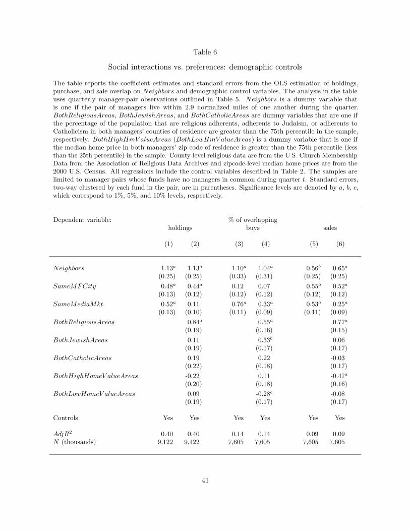
Table 6

Social interactions vs. preferences: demographic controls

The table reports the coefficient estimates and standard errors from the OLS estimation of holdings,purchase, and sale overlap on Neighbors and demographic control variables. The analysis in the tableuses quarterly manager-pair observations outlined in Table 5. Neighbors is a dummy variable thatis one if the pair of managers live within 2.9 normalized miles of one another during the quarter.BothReligiousAreas, BothJewishAreas, and BothCatholicAreas are dummy variables that are one ifthe percentage of the population that are religious adherents, adherents to Judaism, or adherents toCatholicism in both managers’ counties of residence are greater than the 75th percentile in the sample,respectively. BothHighHmV alueAreas (BothLowHmV alueAreas) is a dummy variable that is one ifthe median home price in both managers’ zip code of residence is greater than the 75th percentile (lessthan the 25th percentile) in the sample. County-level religious data are from the U.S. Church MembershipData from the Association of Religious Data Archives and zipcode-level median home prices are from the2000 U.S. Census. All regressions include the control variables described in Table 2. The samples arelimited to manager pairs whose funds have no managers in common during quarter t. Standard errors,two-way clustered by each fund in the pair, are in parentheses. Significance levels are denoted by a, b, c,which correspond to 1%, 5%, and 10% levels, respectively.

Dependent variable: % of overlappingholdings buys sales

(1) (2) (3) (4) (5) (6)

Neighbors 1.13a 1.13a 1.10a 1.04a 0.56b 0.65a

(0.25) (0.25) (0.33) (0.31) (0.25) (0.25)

SameMFCity 0.48a 0.44a 0.12 0.07 0.55a 0.52a

(0.13) (0.12) (0.12) (0.12) (0.12) (0.12)

SameMediaMkt 0.52a 0.11 0.76a 0.33a 0.53a 0.25a

(0.13) (0.10) (0.11) (0.09) (0.11) (0.09)

BothReligiousAreas 0.84a 0.55a 0.77a

(0.19) (0.16) (0.15)

BothJewishAreas 0.11 0.33b 0.06(0.19) (0.17) (0.17)

BothCatholicAreas 0.19 0.22 -0.03(0.22) (0.18) (0.17)

BothHighHomeV alueAreas -0.22 0.11 -0.47a

(0.20) (0.18) (0.16)

BothLowHomeV alueAreas 0.09 -0.28c -0.08(0.19) (0.17) (0.17)

Controls Yes Yes Yes Yes Yes Yes

AdjR2 0.40 0.40 0.14 0.14 0.09 0.09N (thousands) 9,122 9,122 7,605 7,605 7,605 7,605

41

Table 7

Social interactions and manager characteristics

The table reports the coefficient estimates and standard errors for the OLS estimation of measures of portfolio overlap onNeighbors and interactions of Neighbors with various manager characteristics. The dependent variable for the regression resultsdisplayed in columns 1 through 4 is the percentage of overlapping stock holdings between of the funds managed by a givenpair of managers and for columns 5 through 8 the dependent variable is the percentage of overlapping stock purchases betweenthe funds managed by a given pair of managers during the quarter. NeighborTenure is the length of time in years that twomanagers have lived within 2.9 normalized miles of one another. SimilarAge is a dummy variable that is one if the difference inthe managers’ ages is less than the median in the sample (10 years). SameEthnicity is a dummy that is one if the surnames ofthe managers are of the same minority ethnicity. See the appendix for a description of the algorithm used to determine ethnicitiesof surnames. SameCollege is a dummy variable that is one if both managers attended the same college or university. Collegeattendance data are from Morningstar. BothExp (BothInexp) is a dummy variable that is one if both managers have more(less) portfolio management experience than the median manager in the sample. All regressions include the control variablesdescribed in Table 2 as well as the levels of all included manager characteristics (not reported). The samples are limited tomanager pairs whose funds have no managers in common during quarter t. Standard errors, two-way clustered by each fund inthe pair, are in parentheses. Significance levels are denoted by a, b, c, which correspond to 1%, 5%, and 10% levels, respectively.

Dependent variable: % of overlapping holdings % of overlapping buys

(1) (2) (3) (4) (5) (6) (7) (8) (9) (10)

Neighbors 0.79a 0.97a 1.06a 0.81a 0.80b 0.63c 0.67 1.04a 0.49 0.09(0.28) (0.32) (0.25) (0.29) (0.35) (0.37) (0.43) (0.33) (0.33) (0.35)

Neighbors×NeighborTenure 0.19c 0.25c

(0.11) (0.15)

Neighbors× SimilarAge 0.24 0.75(0.36) (0.48)

Neighbors× SameEthnicity 3.73a 2.61c

(1.13) (1.55)

Neighbors× SameCollege 1.03c 1.09(0.57) (1.00)

Neighbors×BothExp 1.12b 3.16a

(0.46) (0.64)

Neighbors×BothInexp -0.51 -0.62(0.49) (0.44)

Controls Yes Yes Yes Yes Yes Yes Yes Yes Yes Yes

AdjR2 0.40 0.40 0.40 0.40 0.39 0.14 0.14 0.14 0.13 0.13N (thousands) 9,122 9,122 9,122 6,296 7,307 7,605 7,605 7,605 5,212 6,069

42

Table 8

Social interactions and stock characteristics

The table reports the coefficient estimates and standard errors from the OLS estimation of various measures of portfolio overlap inholdings (columns 1 through 4) and in purchases (columns 5 through 8) split by various stock-level characteristics on Neighbors,SameMediaMkt, and SameMFCity. Included in the regressions, are the control variables from Table 2, but their coefficient estimatesare not reported. Also, reported is the average overlap in the sample for the dependent variable. A stock is categorized as local if itsheadquarters is within 50 miles of the headquarters of either fund in the fund pair. All other stocks are non-local. Following Hong andKostovetsky (2012), politically sensitive stocks are those in the the Tobacco, Guns and Defense, or Natural Resources industries; allothers are categorized as non-politically sensitive. High (low) analyst coverage stocks are those whose analyst coverage is greater (less)than the median in the sample each year. High (low) advertising expense stocks are those whose advertising expense is greater (less)than the median in the sample each year. Lottery stocks are defined as in Kumar (2009). All stocks that do not meet the definitionare categorized as non-lottery stocks. The analysis in the table uses quarterly fund-pair observations for the sample of 4.2 millionholdings overlap observations and 3.5 million purchase overlap observations from 1996 through 2010. Stocks with missing characteristicinformation are omitted from the analysis. The samples are limited to fund pairs with no managers in common during quarter t.Standard errors, two-way clustered by each fund in the pair, are in parentheses. Significance levels are denoted by a, b, c, whichcorrespond to 1%, 5%, and 10% levels, respectively.

% overlapping holdings % overlapping buys

Same Same Avg. Same Same Avg.Neighbors MediaMkt MFCity overlap Neighbors MediaMkt MFCity overlap

local stocks -0.23a 0.22a 0.06 0.88 -0.21a 0.19a -0.0 0.78(0.08) (0.04) (0.06) (0.06) (0.04) (0.05)

non-local stocks 0.95a 0.06 0.22b 5.77 0.90a 0.39a -0.10 6.15(0.20) (0.09) (0.10) (0.24) (0.08) (0.10)

politically sensitive stocks -0.00 0.02a 0.02a 0.11 0.01 0.01 0.03a 0.12(0.01) (0.01) (0.01) (0.02) (0.01) (0.01)

non-politically sensitive stocks 0.96a 0.35a 0.37a 7.67 1.00a 0.74a -0.05 7.74(0.25) (0.12) (0.12) (0.32) (0.10) (0.12)

S&P 500 stocks 0.86a 0.24c 0.33a 6.75 0.81a 0.52a -0.04 6.24(0.25) (0.12) (0.13) (0.28) (0.10) (0.11)

non-S&P 500 stocks 0.19b 0.13a 0.15a 1.22 0.30b 0.24a 0.09b 1.86(0.09) (0.02) (0.03) (0.14) (0.03) (0.04)

high analyst cov. stocks 1.02a 0.35a 0.48a 7.91 1.08a 0.74a 0.03 7.98(0.25) (0.12) (0.13) (0.33) (0.11) (0.12)

low analyst cov. stocks 0.03a 0.01a 0.01b 0.07 0.03 0.02a 0.02a 0.13(0.01) (0.00) (0.00) (0.02) (0.01) (0.01)

high advert. exp. stocks 0.38a 0.06 0.31a 3.70 0.37b 0.22a 0.09 3.56(0.14) (0.07) (0.07) (0.17) (0.06) (0.06)

low advert. exp. stocks 0.00 0.01a 0.01a 0.09 0.03 0.02a 0.01 0.14(0.01) (0.00) (0.00) (0.02) (0.00) (0.01)

lottery stocks 0.01b 0.01a 0.01a 0.04 0.04b 0.02a 0.03a 0.09(0.01) (0.00) (0.00) (0.02) (0.00) (0.00)

non-lottery stocks 1.04a 0.36a 0.47a 7.94 1.06a 0.74a 0.03 8.01(0.25) (0.12) (0.13) (0.33) (0.11) (0.12)

43

Table 9

The performance effect of social interactions: Holdings

The table reports returns for “neighbor” (N) and “non-neighbor” (O) holdings of fund managers. Theneighbor portfolio of fund i contains those stocks in the fund’s portfolio that are also held by at leastone other fund managed by a manager who lives in the neighborhood of at least one of the managersof fund i. Holdings that do not meet this criterion comprise the non-neighbor portfolio. We use theperformance measures

RNi,t =

∑k∈N

(wi,k,t∑

k∈N wi,k,t

)rk,t+1,

and

ROi,t =

∑k∈O

(wi,k,t∑

k∈O wi,k,t

)rk,t+1,

to calculate the neighbor and non-neighbor returns, respectively, each quarter by averaging acrossfunds in quarter t, weighting each fund’s return by its total net asset value. (N denotes the set ofneighbor stocks, O is the set of non-neighbor stocks, and wi,k,t is the actual portfolio weight of fundi in stock k during quarter t.) Columns 2 and 3 report the raw and risk-adjusted returns for theneighbor and non-neighbor portfolios. Risk adjustment is based on DGTW. Column 4 reports thedifference in returns between these portfolios, and the results of the paired t-test testing whether thedifference is significantly different from zero. Standard errors are reported in parentheses. Significancelevels are denoted by a, b, c, which correspond to 1%, 5%, and 10% levels, respectively.

RN RO RN −RO

Excess return 0.61 0.55 0.06(0.49) (0.47) (0.68)

DGTW (entire CRSP universe) 0.10 0.06 0.04(0.08) (0.08) (0.11)

DGTW (CRSP with price>$5) 0.02 0.00 0.02(0.08) (0.09) (0.12)

44

Table 10

The performance effect of social interactions: Trades

This table reports the investment performance of mutual fund trades. We form portfolios at the beginning of eachquarter based on whether the fund bought or sold a stock, respectively. Stocks that are bought are aggregatedinto the “buy” portfolio, while those that are sold during the quarter are placed in the “sell” portfolio. We createtwo additional subgroups within the buy and sell portfolios: “neighbor” (N) and “non-neighbor” (O) trades. Tocalculate the value-weighted quarterly returns of the neighbor and non-neighbor buy and sell portfolios, we thenaverage the returns of each subportfolio in each quarter across the funds in our sample using the dollar assets(TNA) of each fund in the previous quarter as weights. Columns 1 and 2 report the risk-adjusted average returnsof the neighbor buy and sell portfolios, respectively. Risk adjustment is based on DGTW. Columns 4 and 5 reportthe corresponding results for the non-neighbor portfolios. Finally, columns 3 and 6 describe the difference ofthe returns of the buy and sell portfolios for the neighbor and non-neighbor stocks, respectively, and column 7provides the difference-in-difference estimate. Standard errors are reported in parentheses. Portfolio returns arereported for the entire sample period and a sample period that excludes the financial crisis; as well as for 1) allfund transactions, 2) extensive margins, and 3) intensive margin transactions. Significance levels are denoted by a,b, c, which correspond to 1%, 5%, and 10% levels, respectively.

DGTW-adjusted monthly returns

Neighbor portfolio Non-neighbor portfolio

Buys Sells Diff. Buys Sells Diff. Diff.-Diff.

All trades

Full sample 0.21 -0.27 0.48b 0.10 0.10 0.01 0.48b

(0.16) (0.17) (0.23) (0.11) (0.10) (0.15) (0.24)

Excluding the financial crisis 0.32c -0.30 0.62b 0.16 0.04 0.12 0.49c

(0.19) (0.20) (0.28) (0.13) (0.11) (0.17) (0.28)

Extensive margin trades

Full sample 0.25 -0.73b 0.99b 0.22 0.34 -0.12 1.11b

(0.23) (0.32) (0.40) (0.17) (0.21) (0.27) (0.42)

Excluding the financial crisis 0.37 -0.92b 1.30a 0.21 0.34 -0.13 1.43a

(0.26) (0.39) (0.47) (0.21) (0.23) (0.31) (0.48)

Intensive margin trades

Full sample 0.27c -0.13 0.40c 0.03 0.06 -0.03 0.43c

(0.16) (0.18) (0.24) (0.13) (0.12) (0.18) (0.25)

Excluding the financial crisis 0.37b -0.11 0.48c 0.09 0.02 0.07 0.41(0.18) (0.21) (0.28) (0.15) (0.13) (0.20) (0.29)

45

Figure 1: City clusters and close manager pairs

The figure shows the geographic dispersion of fund managers. Residences are identified by zip codes, and we use a clustering algorithm togroup nearby zip codes into cities, as explained in the main text. The algorithm stops joining clusters that are more than 50 miles apart. Thesize of the circle is determined by the number of unique managers who have a residence in the city at some point during our sample period,while the shaded pie slice indicates the proportion of managers who are close to at least one other manager at some point during the sampleperiod. Managers are classified as close if they live within 2.9 normalized miles of each other, where the normalization adjusts for populationdensity (see text for details).

46

Figure 2: Manager distance and portfolio overlap

The figure plots abnormal portfolio overlap in holdings and purchases for all fund pairs and for fundpairs with single managers as a function of the distance between the residences of the funds’ managers.For distances of less than five miles, we use the population density-adjusted driving distance, asexplained in the text; larger distances are not adjusted and are computed using the distance between thegeographic centers of zip codes. Abnormal overlap is the remaining portfolio overlap after controllingfor funds matching on Morningstar size or value/growth categories (BothSmallCap, BothMidCap,BothLargeCap, BothV alue, BothGrowth, BothBlend), funds being from the same mutual fund family(SameFundFam), and funds having at least one pair of of managers that manage at least one otherfund together (MngOtherFundTogether). It is estimated using all fund pair observations, excludingthose fund pairs with at least one manager in common as in columns 5 and 8 of Table 2 and columns 2and 4 in Table 3. Standard errors are shown as error bars.

47

Coefficient estimate (bps)

Fre

quen

cy

−40 −30 −20 −10 0 10 20 30 40 50 60 70 80 90 100 110

050

100

150

200

250

300

350

Neighborscoefficient estimate

from Table 2, column 5

Mean estimate: Med. estimate: St. dev. of estimates: 0.5 percentile: 99.5 percentile:

8.8 bps8.8 bps

13.7 bps−26.2 bps

43.9 bps

Figure 3: Bootstrap analysis

The figure shows the distribution of Neighbors coefficient estimates from 5,000 bootstrap simulations ofthe regression equation in Table 2, column 5. We impose the null of no neighbor effect by randomizingwho is a neighbor. If a manager pair observation is in the same media market (SameMediaMkt = 1), werandomly assign the pair to be neighbors with probability 3.5%, which gives the same overall proportionof neighbors as in the sample. The sample coefficient estimate is approximately 7 standard deviationsgreater than zero.

48