The Pantanal-Taquari project: Decision Support System for catchment-based river management.

Final Report Programme Partners for Water.

September 2004.

ITC-Enschede-The Netherlands

Dr. B.H.P. Maathuis

Table of Content 1 Introduction 1 2 Activities conducted 1 2.1 Outline of main activities 1 2.2 Outline of main in-house activities 1 3 Data collection and processing 1 3.1 Remote sensing data 1 3.2 Maps and reports 2 3.3 Elevation data 2 3.4 Data collected at Embrapa in August 2003 3 4. SRTM digital elevation model processing 4 4.1 Upper Taquari catchment 4 4.2 Lower Taquari river 4 5 Other sources of information 5 6 Field campaign April 2004 8 6.1 Objectives of the field survey 8 6.2 Equipment used for the survey 8 6.3 Type of data collected 8 7 Analysis of collected data 9 7.1 Sounding measurements 9 7.2 DGPS measurements 10 7.3 Other measurements and observations 10 8 Final DEM processing 13 8.1 Absolute accuracy assessment of the SRTM-DEM and DGPS

measurements 13 8.2 DEM filtering versus use of remote sensing based land use and land cover information 13 8.3 DEM processing 15 8.4 DEM hydro optimization procedures 16 8.5 DEM model run differences 17 8.6 DEM accuracy assessment 20 8.6.1 Absolute assessment 20 8.6.2 Relative assessment 21 9 Conclusions 25 10 References 27 11 ARCVIEW project 29 Appendix 1: Remote sensing image analysis and altitude determination of the Rio

Taquari – Pantanal system Appendix 2: SRTM – derived DEM: Optimization for hydrologic modeling Appendix 3: Pantanal digital terrain model Appendix 4: DEM processing model runs 1 - 4. Full details Appendix 5: Poster: SRTM derived DEM for the Pantanal, Brazil

List of figures 1 Pattern of scanned points using an oscillating mirror 7 2 Track record and (measured – obtained) DGPS locations along

the Taquari 9 3 DEM computation using hierarchic robust interpolation 14 4 Drainage optimization parameters used 17 5 The Caronal avulsion 18 6 Sounding measurements Taquari and Caronal avulsion 18 7 Lineaments identified crossing the Pantanal region 19 8 Run 4 model results 20 9 Extracted drainage 21 10 DEM of the Caronal region 21 11 DEM difference map and satellite image window 22 12 Processed DEM and satellite image window Caronal avulsion 23 13 Processed DEM and satellite image window Paraguay floodplain 23 14 Spatial distribution of elevation differences computed 24 15 The final DEM obtained 24

List of tables 1 Laser scanning activities in Brazil 6 2 Typical mission parameters 7 3 SRTM versus DGPS measurements 13 4 Model run 1 15 5 Model run 2 16 6 Model run 3 16 7 Model run 4 16 8 Absolute errors SRTM-DGPS-hydro processed DEM 20

7

Acknowledgements I would like to acknowledge a number of persons and organizations for their contribution to complete the work presented in this report. For the field survey use was made of sounding and DGPS equipment. The method for quick bathymetric surveys using portable sounder linked to GPS and integration with GIS was developed by Mr. Ing. Remco Dost from the Department of Water Resources, ITC. The dual frequency GPS used was provided by Drs. Klaas Verwer, Department of Sedimentology, Free University of Amsterdam. Furthermore I would like to express my thanks to Roberto de Ruyver MSc from Argentina who was instrumental in developing the appropriate correction procedures for hydro-DEM optimization. Also the ILWIS development team at ITC is thanked for their effort in programming the necessary routines and algorithms needed for DEM hydro-processing. Thanks also go to the Dutch project team members from Alterra en WL-Delft Hydraulics, especially the collaborate effort to collect a large amount of data of the Taquari during the very interesting but tough field survey. Their attitude was highly appreciated. I would like to express my sincere thanks to Mr. Carlos Padovani of the Corumba office of Embrapa. The data provided and his assistance, both in the field and “online”, were essential to complete the assigned tasks. Other persons from Embrapa, like the boatsmen, are thanked for their assistance as well as their keen interest during the visit to Corumba and the fieldwork in the Pantanal. Finally I want to thank Dr. Rob Jongman and Ir. Marion Bogers for their coordinating role within this project.

8

1 Introduction. The overall objective of this project is to support the wise use of the plains of the Pantanal Taquari river catchment by developing tools for decision making in river management at the catchment basis. With regard to this two problems are of main importance, the first: the development of a river flow and sedimentation model of the lower Taquari in the Pantanal and improve the Brasilian knowledge in this matter. Second is the capacity building for the organization of integrated river management at the catchment level including all relevant stake holders. This report mainly focuses on the first problem identified and describes those aspects that have contractually been assigned to ITC. In this respect, apart from participation in relevant project activities, the main focus was on the preparation of a digital terrain model (DEM) to facilitate further hydro-dynamic modeling by other partners.

2 Activities conducted. 2.1 Outline of main activities

1. Remote sensing data collection, initial analysis and preparation of presentation. 2. Participation in the 1st workshop on the Taquari-Pantanal Project, Corumba,

19-20 August 2003. A presentation was given entitled: Remote sensing image analysis and altitude determination of Rio Taquari-Pantanal system (appendix 1).

3. Additional data collection and short field survey directly after the 1st workshop. 4. Attending 2 project meetings (coordinating the Dutch partner effort) at Alterra

in Wageningen and giving a presentation of ongoing activities entitled: SRTM-derived DEM: Optimization for hydrologic modeling (appendix 2).

5. Participating in a joint fieldwork in April 2004 to collect additional data on the Taquari river from Coxim to Corumba using several techniques.

6. Processing the collected data and presenting the obtained results in a presentation at Alterra entitled: Pantanal Digital Terrain Model (appendix 3, 4).

7. Disseminating the processed data to Alterra. 8. Preparation of a poster presentation showing the obtained results for the

closing workshop in Corumba (appendix 5). 2.2 Outline of main in-house activities

1. Testing of specially developed software routines for DEM hydro-processing. 2. Acquire dedicated DEM filtering software and processing the Pantanal DEM

through different model runs with different parameter settings. 3. Supervising MSc study related to Hydro-DEM processing. 4. Integration of sounding-surveys and GIS. 5. Single dual frequency geodetic (D)GPS recording and post-processing

procedure development applicable to the Pantanal field conditions.

3 Data collection and processing Prior to the first workshop most attention was given to data collection. 3.1 Remote sensing data An inventory was made of available remote sensing data of the Pantanal region as well as elevation information. This was done using international archives as well as the in-house available digital archive (Geo-data warehouse) and analog archive. This resulted in a large amount of remote sensing images, available from different sensors

9

from 1973 onwards, such as Landsat-MSS and TM, Aster, JERS. Furthermore some aerial photos from the analog archive were available (covering small portions of the Paraguay river floodplain). Details are as follows:

• Landsat MSS data from 15 and 16 March 1973. • Landsat TM images from 1986 till 1989, dry season conditions.

Excellent quality, whole Taquari catchment at 30 m. spatial resolution, 7 spectral bands. Total of 11 scenes. A mosaic of 9 scenes is covering the lower Taquari and 4 scenes cover the upper Taquari catchment.

• Aster (onboard of EOS AM-1) images from 2000 till beginning of 2003, dry season conditions, partly cloud covered; only covering the lower Taquari. Visible and near infrared images at 15 m. spatial resolution, 3 spectral bands. 95 scenes are available; a mosaic has been made from 25 selected scenes.

• JERS (radar L-band, 23 cm centre wavelength, HH polarization): mosaic of February 1997, showing wet season conditions, resampled to 100 m. spatial resolution, mosaic from 50 JERS-1 scenes.

As the Pantanal region is very extensive only a mosaic consisting of several individual images can cover the whole area. Given the revisit time of these medium resolution satellites, coupled with occurrences of clouds, a mosaic can only be constructed from images acquired over a longer period of time. Therefore the flooding phenomena depicted on the individual images differ strongly. The JERS data are acquired within a specific period, but the spatial resolution to which the mosaic is resampled makes it less useful. 3.2 Maps and reports Some 1:50.000 scale maps covering part of the Paraguay floodplain region, next to general small scale maps, were obtained. Also some relevant older reports of the Pantanal area could be obtained. 3.3 Elevation data Apart from the GTOPO30 (30 arc-second DEM, roughly 1 km spatial resolution) the elevation data that could be acquired of the whole region is from the Shuttle Radar Topographic Mission (SRTM) of February 2000. Data are collected from the space shuttle Endeavour which was launched on 11 February 2000, during an 11 days mission from an orbital altitude of 233 km using a modified radar instrument called the Spaceborne Radar Laboratory, with an Interferometric Synthetic Aperture Radar (IFSAR), two C-band antenna’s (centre wavelength 5.3 cm), one of which was mounted on a 60 m. mast, the other was situated in the cargo bay. The SRTM swaths extended from about 30 degrees off-nadir to about 58 degrees. The spatial resolution available is 90 m (3-arc-seconds at equator is 90 m), which is downsampled using a 3 by 3 averaging filter algorithm from the original 30 m. resolution data (1 arc-second). Since the primary error source in the elevation data has the characteristics of random noise, this reduces that error by roughly a factor of three. The vertical resolution is 1 m. having an absolute accuracy of better than 16 m (90 % confidence level). Data are processed in one degree by one degree cells. In order to cover the Taquari catchment a mosaic was constructed of 40 tiles, covering an area from 16 degree South / 59 degree West (upper left corner) to 21 degree South / 53 degree West (lower right corner). More details on processing of the DEM is provided below.

10

3.4 Data collected at Embrapa in August 2003 After the 1st workshop at the Embrapa office in Corumba the following data could be obtained: Satellite data:

• SAC-C images from 08 Aug ’01, 04 March ’02, 28 September ’02 and 24 April ’02. This sensors spectral resolution of the 5 bands is identical to Landsat TM, spatial resolution is 180 m.

• A mosaic of Landsat TM, representing the dry season conditions as of 1998-1999, transformed to a pseudo natural colour, in 30 m. and 180 m. resolutions (VNIR-R-G transformed to RGB).

GIS data: • Scanned topographical maps 1:250.000. • Collection of GIS data based on the 1:100.000 scale topographical

maps in a data format that can be accessed by the software SPRINGS. • A collection of exported files from SPRINGS in an ARC-shape file

format. Next to this, during the one day field visit, field photos were collected as well as site observations.

4 SRTM Digital Elevation Model processing 4.1 Upper Taquari catchment- the Plateau (Planalto) First the quality of the SRTM elevation data was evaluated using the Taquari catchment area upstream of Coxim. Small data voids (e.g. along some portions of very steep, nearly vertical escarpments) were linear interpolated. In general no further correction was adopted as the area was properly recorded and is having substantial elevation differences. Apart from this the area is extensively used for agriculture and cattle ranging, some small regions are covered by natural open savanna vegetation. Only along the escarpments a dense forest cover is located. Given the type of land use and cropping patterns for the area in relation to the date of acquisition, nature of interaction at the surface given the wavelength used of the active radar signal to collect the elevation information is was assumed that for major portions of the upper catchment region the elevation data is representing the actual ground levels. To extract relevant hydrological parameters the elevation data was processed using different software packages and extensions such as:

• ARCVIEW HEC- GeoHMS extension; • ARCGIS Hydro-tools extension and Taudem extension; • DiGeM (dedicated free software tool for digital terrain analysis); • At a later stage the ILWIS Hydro-tools module (self developed

software tools for DEM processing).

Especially the ARCGIS-Taudem extension facilitated the processing and extraction of hydrological parameters, such as river network and (sub) catchments of good quality next to the more generic variables as slope and aspect. Visually the results could be compared to available satellite images and the drainage lines extracted were superimposed on these images. DiGeM allowed for the calculation of a number of compound terrain parameters such as (1) the Wetness index (catchment area / slope gradient) showing the spatial distribution of zones of saturation and variable sources

11

of runoff generation, (2) Stream Power index (catchment area * slope) showing areas susceptible to concentrated surface runoff and (3) LS or Transport index accounting for the effect of topography on erosion (using catchment area instead of the one-dimensional slope factor as in the USLE). Also the first test runs were conducted with the ILWIS hydro-tools module, showing similar results as with the Taudem extension. The information obtained, together with satellite data, is useful in the analysis of upstream-downstream relationships envisaged by the other project team members. Examples of these compound index maps are provided in appendix 1. 4.2 Lower Taquari river - the Pantanal Using the same procedures the raw SRTM data was processed of the lower Taquari reach. Given the completely different terrain characteristics (from Coxim the Taquari traverses an alluvial fan complex before it enters into the wetlands - marshes) these initial results were not successful. This was basically due to two reasons: (1) the strong influence of the reflectivity – backscatter of the radar signal by the top of the natural vegetation and (2) due to the fact that the radar signal does not penetrate water, so therefore no bathymetric information, extremely important for the lower Pantanal region, was incorporated in the data source. Prior to the field survey, in order to see how the SRTM data could be modified a DEM optimization routine was developed and tested. The routine is consisting of several steps and is discussed into more detail below:

1. In order to remove the effect of vegetation the SAC-C image of 8 Aug 2001 (bands 3 and 4) was selected and a Normalized Difference Vegetation Index (NDVI) was calculated. It was assumed that higher NDVI values were corresponding to higher vegetation structures, like bushes and trees. The NDVI map was reclassified into elevation classes and subsequently subtracted from the initial DEM.

2. To incorporate the bathymetric information of the extensive drainage network existing in the Pantanal a drainage network layer, taken from the 1:100.000 scale topographical maps by Embrapa was used. This drainage map was corrected and updated (especially along map boundaries) using the pseudo natural color mosaic also obtained from Embrapa. The corrected drainage system was reclassified into three classes, representing the Paraguay river, the Taquari river and the other drainage network. Different values are used to represent the width and depth of these rivers. The DEM corrected for vegetation influence was modified once more to represent the drainage network as well. In order to obtain a consistent flow direction and accumulation network the drainage was incised with values over representing the actual river depth. In a subsequent step the differences (reclassified into a number of classes) between the original DEM and the drainage incised DEM was used to raise the actual riverbed levels. The then newly computed flow direction and flow accumulation resulted in a hydrological sound drainage network when compared to the network as it is depicted on the satellite images

3. Last but not least a multi-temporal classification of all 4 SAC-C images was conducted and a flood extent map was produced, showing the areas continuously flooded up to occasional flooded and non flood affected. Apart from the river system, based on the flood frequency a depth value was assigned and this was once more used to correct the DEM

12

These three steps (in the given sequence) completed the initial DEM correction procedure. Main problems encountered during this process were:

• NDVI is not a good representation of vegetation, also areas covered with e.g. dense grass, water hyacinth produce high NDVI values.

• Visual interpretation of the drainage network from the satellite images is very difficult for the lower Pantanal region, small diversions and avulsions are not well depicted. Furthermore the drainage network was not recorded at bank full stage.

• Information with regard to bathymetry was not available and was assumed. Even after raising the river bed levels these were considered still too deep. Also the values used for correction of flood affected areas were assumed.

• Sequence of DEM correction is important because sink-fill operators, prior to the flow direction and flow accumulation computation affect the results.

• The modified DEM at this stage could only be validated in a relative way as no absolute elevation information (X,Y,Z) was available in the used ellipsoid and datum and transformation parameters were unknown.

Therefore the results had a preliminary character and had to be further validated during a planned field campaign. A presentation highlighting the proposed modification procedure is given in appendix 2.

5 Other sources of elevation information Next to the C-band SRTM elevation information, on board of the same space shuttle mission, a X-band radar was installed (centre wavelength 3.1 cm). The processed X-band elevation information is available (at the German Space Agency, DLR) at higher spatial resolutions (30 m). The X-band data is nested within the C-band swath (X-band swath width is 50 km), and has therefore not fully covered the Pantanal region. The accuracy specifications are: absolute vertical accuracy better than 16 m. and relative accuracy better than 6 m. The cost of a single 15 by 15 minutes tile is approximately Euro 500. Purchase of X-band elevation information of a substantial area was considered not feasible within the scope of this project. Other Interferometric SAR sources (IFSAR-INSAR), e.g. using RADARSAT (F1- fine beam) or ERS Single Look Complex data, reported horizontal accuracies of 10 and 20 m. respectively and absolute vertical accuracies between 5 to 15 m (assuming 5 or more accurate ground control points are provided) or optical stereoscopic means, both space - and air borne based (SPOT, ASTER across and along track images and traditional aerial photography, using parallax differences in the overlapping image portions) could be applied, but the main limitation using this approach is the amount of fieldwork involved to acquire a sufficient number of high quality ground control points to make sure that the extracted DEM would meet accuracy standards. Another limitation with regard to INSAR-IFSAR is that the dielectric properties of the area are prone to be different considering the time interval between the moments of image acquisition from different orbits, which will seriously affect the coherence between the images and therefore the DEM output quality. As is the case with X-band SRTM elevation information, to acquire and process the remote sensing data to obtain an elevation model, would mean a huge investment.

13

Airborne laser scanning (ASL): Another approach to collect detailed elevation information using remote sensing techniques is by means airborne laser scanning. Absolute horizontal and vertical accuracies are reported in the cm range, slightly larger absolute vertical errors exists when high vegetation is encountered, but in general the RMSE is still less than 0.5 m. Esteio Engineering and Aerosurveys Inc., situated in Curitiba, was the first company in Brazil to acquire a laser scanner in 2001. In the mean time another specialized company in cartography (GEOID Ltda) and a technology institute for development (LACTEC) linked to the Federal University of the State of Paraná and the Power Company of the State of Paraná started airborne laser scanning activities in 2002. Details are given in the table 1. These companies – institute use ALS not only for traditional DEM collection for image ortho-rectification purposes but also for electric power transmission line surveys, highway engineering, surveying areas of interest for hydraulic potentials (reservoir capacity calculations), detailed surveys of mining areas, forest (biomass) resources inventory, urban mapping, etc. The Optech’s ALTM series of laser scanners – receivers - software is capable to acquire the first and last pulse of a measurement simultaneously; therefore it can measure both the tree- or vegetation heights as well as the topography of the ground beneath in a single pass. A frequency of e.g. 25 kHz indicates that 25.000 height measurements per second can potentially be collected. Furthermore, next to the ranging information, the system can categorize the detected laser pulses according to the reflectivity of the target surface as high reflective materials provide a strong (intense) return signal. This results in an intensity image showing great similarity to a panchromatic or black and white image – photo, allowing to identify the different types of ground features recorded during the over flight. This facilitates a better assessment of the filtering algorithms and the results obtained. Table 1: Laser scanning activities in Brazil Company/Institution ESTEIO S.A. GEOID Ltda LACTEC System - Model ALTM 2025 ALTM 1225 ALTM2050 Manufacturer Optech Inc. Optech Inc. Optech Inc. Maximum flying operational altitude

2000 m. 1200 m. 2000 m.

Laser scanner frequency

25 kHz 25 kHz 50 kHz

Year of acquisition 2001 2002 2002 A typical ground scanning pattern using an oscillating mirror system and flight envelope – scanning results for an Airborne Laser Scanner is given in figure 1 and table 2 below showing the influence of adapting some of the flight parameters – variables. From the table below it is clear that this technique, although operational in Brazil, has limited potentials to construct a detailed digital elevation model of the whole Pantanal region. To record a reasonable area and process it into a digital terrain model would require a huge (financial) effort given the narrow swath width covered using a reasonable scan angle (at larger scan angles more and more laser points are trapped within the upper portion of the vegetation). Furthermore it should be noted that the necessary bathymetric information of the fluvial system is not collected, as water is

14

not opaque for the near infrared signal used (some scanners operate in the visible green wavelength region, making water transparent to a certain degree depending on the suspended sediment concentration). Last but not least, even if a highly accurate elevation model is available, e.g. of the Caronal avulsion area, also other model input parameters should be known, such as detailed (time series of) hydrological and sedimentological data, in order to successfully apply a hydro-dynamic model. This is also a serious limitation for the Taquari-Pantanal region. Figure 1: Pattern of scanned points using an oscillating mirror

V = Aircraft speed (m/s)Fp = Pulse emission frequency L = Swath widthH = Flying height (minimum 300 m maximum 2000 m)A = Scan angle (maximum +/- 20°)Sp = Point spacing perpendicular to the flight path (m)Sd = Point spacing in direction of flight (m)Fs = Laser scanner frequency

L = 2 * H * tan (A) Sp = 2 * L * Fs / FpSd = V / (Fs*2)

L

Sp

Sd

Table 2: Typical mission parameters

4018.2 m1 m

Points –scan lineSpSd

404.4 m1 m

Points –scan lineSpSd

Scan rate 25 Hz

1007.2 m2.5 m

Points –scan lineSpSd

1001.8 m2.5 m

Points –scan lineSpSd

Scan rate 10 Hz

2003.6 m5 m

Points –scan lineSpSd

2000.9 m5 m

Points –scan lineSpSd

Scan rate 5 Hz

Scan Angle = 20 degrees, Scan width = 730 m

Scan Angle = 5 degrees, Scan width = 175 m

Flying height above terrain = 1000 m, ground speed of aircraft = 50 m/s, laser frequency = 2000 Hz

Assumptions

15

6 Field campaign April 2004 From 28 March till 9 April 2004 a field campaign to collect additional information was conducted. 6.1 Objectives of field survey

• Study of the main morphological characteristics of the Taquari river and active floodplain from Coxim to Corumba and collect relevant info for hydro model input.

• Collect relevant field information to correct the Shuttle Radar Topographic Mission Interferometric derived Digital Surface Model (DSM) to be able to convert it to a realistic Digital Terrain Model (DEM) of the Pantanal region.

• Study the terrain features surrounding the river and active floodplain into more detail, especially along the main avulsions, the Caranal and Ze da Costa avulsions.

• Collect multi temporal aerial and satellite image info for change analysis along the sections affected by avulsions.

6.2 Equipment used for survey

1. Leica SR530, RTK (D)GPS and antenna 2. Garmin Fishfinder – transducer (sonar) and Garmin GPS 72 3. Garmin Etrex GPS 4. Laptop (Erdas Imagine, ArcGIS, Arcview, ILWIS, Leica-SKI-Pro and

Gartrip) and a palmtop (Ipaq with ArcPad) 6.3 Type of data collected

1. Sounding and GPS information along the river, the whole section, from Coxim to Corumba, water depth, height and X,Y (UTM, zone 21, WGS84) information, longitudinal profile, 1 point per 10 seconds (approximately 1 point per 80 metres), covering main bed configuration changes within the river and cross-sections, 1 point per 2 seconds (approximately 1 point per 2.5 metres).

2. DGPS measurements, 6 points along the Taquari, 2 along the Paraquay Merin, a point at Corumba harbour, 2 observations on geodetic points at University of Corumba, one from the aviation authority and one from the Department of Geodesy, Brazil (IBGE). Time duration per point between 1 ½ to 2 hours of continuous recording. Data converted to RINEX format for later post processing at SOPAC-SCOUT. Also a geodetic point at ITC was measured for quality control.

3. Sediment samples taken from the river bed using sediment grabber along cross-sections and flow velocities and visual observations for the whole duration of the boat trip (7 days).

All data collected by sounder, (D)GPS were downloaded and pre-processed successfully and exported as Arcview Shape files. The measurements need to be corrected for sounder depth offset (+ 30 cm) and GPS height offset (- 60 cm). General overview of data collected is presented in figure 2 (total river length covered: >400 km.). Sediment samples (17) are given to the laboratory of Embrapa for grain size analysis. Further details are presented below.

16

Figure 2: Track record and (measured – obtained) DGPS locations along the Taquari.

From Centro deCartografia

Own DGPS Measurement

Route takenby boat

Coxim

Corumba

Ze da Costa

Caronal

When plotting all data on pseudo natural color composite Landsat TM background (UTM, zone 21, WGS-84 ellipsoid and datum) there is a good overall match. Other data collected at Embrapa: Landsat ETM images of 04-05-2000 and 29-09-2000 (WRS 227-73 and 226-73), all bands, Aerial photographs (panchromatic, April 1960), recorded in 1960 of the two avulsion areas, scale 1:60.000, corresponding topographic maps of these areas of interest. Furthermore the GPS tracklog of Embrapa (Carlos Padovani) was downloaded and converted to Arcview Shapefiles and integrated together with the preliminary DGPS observations, sounding point and track-log files.

7 Analysis of collected data 7.1 Sounding measurements In order to get a better idea of the Taquari, during the trip from Coxim to Corumba, a transducer – sonar was attached to the back of the boat, about 30 cm below the water level. Water depths are registered using this portable sounder connected to a GPS. The sounder uses a single frequency transductor of 200 kHz to measure the distance from the sensor to the river bed with an accuracy of 10 cm. Minimum recording depth of the water body is 60 cm. Furthermore if there is a high suspended sediment concentration the sounder is not able to take measurements. Most of the cross sectional locations selected had been measured previously by other organizations. Additional cross-sections are selected based on hydro-dynamic model requirements. Horizontal accuracy is depending on the quality of the GPS receiver used, which in this case is in the order of 5 to 10 m. All collected data are transferred from the GPS to the laptop in the field and pre-processed in a GIS (ILWIS) twice a day. The point and track records were integrated with a geocoded satellite image to check the locational consistency of the measurements. At a later stage the data was transformed

17

into a different format in order to be compatible with software packages used by other project partners for further post-processing and analysis. 7.2 DGPS measurements To get an idea of the absolute vertical accuracy of the DEM dual frequency geodetic DGPS static measurements were conducted at several locations along the Taquari. Given the type of survey it was not possible to prepare a base and a rover station for real time accurate position measurements as (1) setting up a base station requires long duration measurements and (2) the distance between the base station and rover is restricted. There is a limiting distance with regard to the radio link between the two stations (no mobile telecommunication network is available in the Pantanal) and with increasing distance (over 10 km) from the base station problems can occur when trying to resolve the ambiguity (N). To overcome this problem also long measurements are needed and measurements become less representative causing larger positional errors, especially vertically (accuracy drops with 1 mm / km). Another possibility, through collection of correction factors using satellite communication by OmniSTAR, was thought to be not accurate enough as the ground stations situated along the coast (Buenos Aires, Curitiba, Rio de Jianero and Vitoria (for which the correction factors are computed - known) are less representative for the Pantanal region causing at best absolute vertical accuracies in the order of 30 to 50 cm. Therefore use was made of a free Internet GPS post-processing service provided by the Scripps Orbit and Permanent Array Center (SOPAC). This center provides precise, rapid, ultra rapid and hourly orbits for the International GPS Service (IGS). The IGS network is consisting of over 200 permanent GPS stations and the three nearest stations are used by the Scrippt Coordinate Update Tool (SCOUT) to process the dual frequency geodetic quality GPS RINEX (Receiver Independent Format file) data observed in static mode and receive rapid turn-around precise coordinates. Solution quality depends largely on the availability and proximity (also called base line) of the nearest three base station data and the availability of precise satellite orbits and clock corrections. To validate the post-processing results two known geodetic points were recorded, next to those in the Pantanal, one point in Enschede, the Netherlands and one in Corumba, Brazil. This resulted in height differences of 2.5 cm (average base line of 130 km) and 11 cm (average base line of 1160 km) for Enschede and Corumba respectively. Given the fact that the average base line length is roughly the same for the other measurements and the duration of measurements was mostly longer than the measurement at the geodetic point in Corumba, the obtained vertical accuracy (in the order of 10 cm) is thought to be representative for the other static dual frequency measurements conducted in the Pantanal. 7.3 Other measurements and observations Other activities conducted during the boat trip included collection of sediment samples taken at locations were cross sections were recorded. At these locations also flow velocities were recorded using the GPS. Furthermore visual observations, to get a better idea of the (changes in) landscape were performed and flood marks were observed.

18

The main river system differences observed are:

• From Coxim till approximately 30 km east of the Caronal avulsion. The Taquari incised the fan surface, is confined to a narrow active floodplain, with levees of about 60 cm in height given the actual water levels during the survey. The vertical escarpments mark the boundary between the floodplain and the fan due to active undercutting of the river. The difference between the fan surface and the river level is in the order of 5 to 6 m. at the entrance of the Taquari into the Pantanal. This difference in elevation is decreasing towards the west and the fan surface disappears gradually. The average longitudinal slope is in the order of 30 cm / km and the river depth in general is exceeding 2.5 m. Furthermore the river width in general is greater than 300 m. The river has a strong meandering pattern and especially in the outer bends is showing frequent signs of active bank erosion. Many cut-off meanders exist in this river reach. The flood marks observed show that only the active floodplain is flood affected. Flood marks are observed at 1.2 to 1.5 m. above the water level. Flow velocities generally exceed 4 - 5 km / hr and the river is carrying suspended sediments. The maximum water levels do not reach the fan surface.

• The reach 30 km east of the Caronal avulsion till approximately the Ze Da Costa avulsion. Here the river is not incised any more. The levees are in the order of 30 cm above the water level. Hardly any signs of river bank (lateral) erosion. The width of the Taquari decreased to less than 200 m. The river depth is in general less than 2 m. The longitudinal slope in this reach is between 20 to 30 cm / km. The meandering pattern has disappeared and the river has become straighter and is showing a more braided appearance with many bars and shallows. In the upper part of this reach a number of avulsions exist, both on the left and right banks of the river, diverting a substantial amount of the river’s discharge. Flow velocities are less, 2.5 to 4 km / hr but still suspended sediments are transported. In general flood marks are situated 10 to 20 cm above the levee surface adjacent the river indicating that large regions are flood affected during high river stage.

• Downstream Ze Da Costa avulsion. Here the longitudinal gradient becomes very gentle, about 10 cm / km. Large lakes are present in this area and given the stage fluctuations of the Paraguay river combined with the small topographic differences the area will be affected by backwater effects from this river. The more anastomosing pattern of the fluvial system in this reach might be attributed to this. Flow velocities recorded during the survey are in the order of 1- 2 km / hr. In general the surveyed reach is having river depths of over 3 m. The amount of suspended sediment has gradually disappeared. Further downstream fossil Paraguay levees are found as well as some older structural outcrops – low hills. Apart from these slightly higher elevated areas the region is prone to extensive flooding

19

With regard to the land use and vegetation the following observations can be made: Stretch along the road from Campo Grande to Coxim. This road passed partly through the upper watershed of the Taquari river (the Planalto, plateau). At some places local erosion features were observed. Most of the area is under soybean and during February is at maturing stage, about 20 cm above surface. At local places, especially at steeper terrain sections degraded forest is found. The nearly vertical sandstone escarpments near Coxim are hardly vegetated, other more gently sloping sandstone sections are covered with forest. The vegetation is well adapted to slight changes in elevation along the river section surveyed. Vegetation (evergreen) within the active floodplain along the river on the levees is more than 10 mtr high, some trees locally more than 15 mtr. Natural vegetation (deciduous) on the fan surface is open and generally lower, about 5 to 10 mtr. A major portion of the fan surface is used for cattle ranging and is composed of extensive grass lands. Near the Caronal avulsion many lakes are found, on the shallow levees dead trees are present; in general the vegetation is 0.5 mtr above the (water) surface composed of grass and reed species. Further downstream at the river banks the vegetation (water hyacinth and a type of reed / tall grass) is actively growing making it difficult to determine the actual river bank. At localized higher portions (e.g. fossil levees which are found extensively due to the frequent river changes) trees are situated. Especially further downstream lakes are covered by water hyacinth.

20

8 Final DEM processing 8.1 Absolute accuracy assessment of the SRTM-DEM and DGPS measurements After the DGPS measurements were post-processed the altitude was compared to the SRTM measurements. According to the SRTM product description the National Geospatial-Intelligence Agency (NGA) and contractors performed quality checks and additional finishing steps. One of these is that lakes of 600 meter or more in length are flattened and set to a constant height and rivers that exceed 183 meters in width are delineated and monotonically stepped down in height. As al measurements are conducted along the Taquari and downstream reaches meeting above criteria it is possible that the altitude values are affected by this SRTM post-processing procedure. Table 3 shows the differences. Table 3: SRTM versus DGPS measurements

The difference given for the first measurement is most probably due to the spatial resolution of the SRTM data. The DGPS measurement was conducted next to the river, about 30 m from the fan. The SRTM value is typically representing the altitude fan surface at that location. Largest deviations occur downstream with measurements conducted along the

Paraguay Merin. For these locations the SRTM has identical altitude values (89 m). The DGPS values are about 9 meter higher. This could be due to the SRTM finishing procedures as indicated above. All in all it can be stated that the absolute height accuracy is far better than the 16 meter (90 % confidence) as was specified for the mission. 8.2 DEM filtering versus use of remote sensing based land use and land cover information The SRTM elevation data are with respect to the reflective surface, which may be vegetation, man-made features or bare earth. In order to successfully extract the real terrain elevation these influences have to be eliminated to obtain the actual elevation model that can be incorporated in the hydro-dynamic model. The first attempt to correct the SRTM data was by means of using an NDVI. It turned out that this method was not capable of correcting the vegetation influence appropriately as the grass and especially the water hyacinth covered areas also produced high NDVI values. Furthermore given the spatial resolution of the SAC-C images no good representation was obtained of the vegetation, especially in complex areas. Another attempt to obtain the vegetation cover was by means of unsupervised classification. It was impossible to assign realistic land cover and land use types to the classes obtained, apart from assigning elevation correction factors. Supervised classification was not possible as not enough ground truth could be collected over the Pantanal area. Another limitation was that the satellite data were acquired over a longer period and are showing different flood stages.

SRTM DGPS Difference

185 178.9971 6.0029159 159.2523 -0.2523139 142.411 -3.411139 139.1613 -0.1613135 138.3255 -3.3255105 111.594 -6.594

89 98.2101 -9.210189 97.9044 -8.904497 99.0996 -2.0996

21

Therefore another approach was followed that is commonly used when processing lidar data. Depending on the data acquisition method gross errors (blunders) can occur in the data. They can be caused by human failure, by miss-matches in correlation programs, by multi path effects or reflections on vegetation and buildings. These points can be either above or below the ground. For airborne laser scanner data the gross errors are typically above the terrain, resulting in a skew distribution of gross errors. It is assumed that the SRTM data exhibit the same characteristics as those acquired by airborne laser scanning means, especially in relation to the similarity in interaction at the earth surface as the altitude of the reflective surface is recorded . The technique of hierarchic robust interpolation allows eliminating those blunders automatically. A graphical representation of the process is given in figure 3. Figure 3: DEM computation using hierarchic robust interpolation

The algorithm is based on linear prediction with individual accuracies for each measurement. It works iteratively. In the first step all points are used to estimate the covariance function of the terrain. The surface is computed with equal weights for all points. This surface runs in an averaging way between ground points and vegetation points. The ground points are more likely to

• be below the averaging surface, • have negative filter values, • have positive residuals.

Whereas the vegetation points are more likely to • be above or on the averaging surface, • have positive filter values, • have negative residuals.

The procedure as given in figure 3 is consisting of a number of steps. In a thin out step a set of points is reduced in its details, the data is thinned out. This is performed on a raster basis. This step is useful for guaranteeing that a good mixture of blunders and terrain points is given. In a sort out step points are compared to a DEM.

22

Therefore, the inputs are two files, a point cloud and a DEM. If the points are within a certain distance from the DEM they are accepted, otherwise they are rejected. In a filter step a model is derived from a set of points which contains gross errors. These gross errors are also called off-terrain points. The aim is to eliminate these gross errors completely and build a ground model with the remaining points. This is possible, if there is a good ‘mixture’ of grossly false points and points free of these errors. In an interpolate step a model is derived from the current data set by linear prediction. The difference to a Filter step is that no gross error detection is possible. This procedure results in an automatic classification of the raw data into terrain and off-terrain points and is subsequently followed by an interpolation routine using only the terrain points identified. Till now it is not reported if these procedures, commonly applied to airborne laser data, have been adapted to successfully correct SRTM data and as such the analysis to construct a DEM of the Pantanal region can de regarded a novel approach using SRTM data. The difference between the original SRTM measurements and the filtered – newly interpolated DEM can be regarded as the vegetation height map. Reclassification of this difference map into a number of height classes can assist in the identification of different vegetation types. 8.3 DEM processing In order to import the data a raster to point conversion was conducted. The centre coordinate for each pixel was determined and together with the corresponding altitude was exported as an X,Y,Z table to be used for further DEM processing according to the procedures described above (a total of 5.9 million regularly spaced points, 90 m apart). The details of the parameters used and the DEM processing results for several runs computed are given in appendix 4. The aggregated results are presented in tables 4 to 7 below. Table 4: model run 1

Legend tables 4 to 7. Thinout 1-2: cell size, method, no. of input points, no. of output points Filter 1-4: cell size, no. of stored grid points, no. of reference points given (single points), average filter values (single points), maximum filter values (single points) Interpolation 1-3: cell size, no. of stored grid points, no. of reference points given (single points), average filter values (single points), maximum filter values (single points) Sortout 1-2: no. of input points, no. of output points

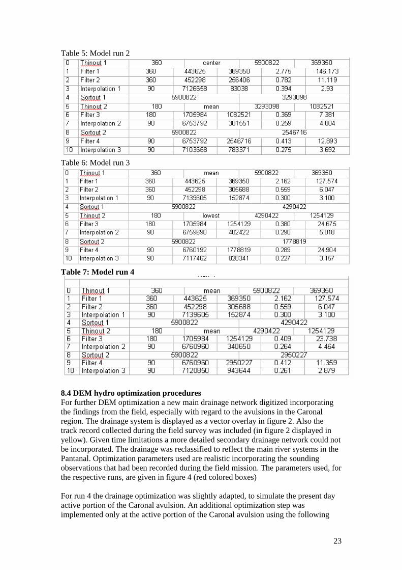
23

Table 5: Model run 2

Table 6: Model run 3

Table 7: Model run 4

8.4 DEM hydro optimization procedures For further DEM optimization a new main drainage network digitized incorporating the findings from the field, especially with regard to the avulsions in the Caronal region. The drainage system is displayed as a vector overlay in figure 2. Also the track record collected during the field survey was included (in figure 2 displayed in yellow). Given time limitations a more detailed secondary drainage network could not be incorporated. The drainage was reclassified to reflect the main river systems in the Pantanal. Optimization parameters used are realistic incorporating the sounding observations that had been recorded during the field mission. The parameters used, for the respective runs, are given in figure 4 (red colored boxes) For run 4 the drainage optimization was slightly adapted, to simulate the present day active portion of the Caronal avulsion. An additional optimization step was implemented only at the active portion of the Caronal avulsion using the following

24

optimization parameters for this small river reach: A, B, C: 180,0,2 respectively. The other optimization parameters are as of run 3. Figure 4: Drainage optimization parameters used

In order to obtain a hydrologically consistent DEM (water is draining to a specified outlet) first possible pits are filled in the DEM (no internal drainage). No control over the fill pit routine was applied resulting in the fact that e.g. a closed depression existing in the DEM would be removed and is “leveled” to the lowest outlet pixel altitude of this local depression. The GIS based flow direction routine used is the Deterministic – 8 procedure followed by a flow accumulation routine. Setting a threshold on the number of contributing pixels to a certain outlet pixel allows for the extraction of the drainage network. This procedure was implemented in ILWIS using a newly developed software routine. In order to evaluate the relative accuracy of the processed and optimized DEM this extracted drainage network can be compared to the drainage from the satellite imagery available. 8.5 DEM model run differences With regard to the DEM processing results of the four runs conducted the following observations can be made with regard to the drainage network extracted:

• Model run 1 is using the (present) inactice Caronal avulsion as the main drainage channel.

• Model run 2 is using the Taquari as its main drainage channel configuration, including the present day drainage configuration as found at the Ze Da Costa avulsion.

• Model run 3 is using the (at present partially artificially blocked) minor avulsions at the left bank of the Taquari, just east of the Caronal avulsion, as its main drainage channel.

• Model run 4 extracts the drainage according to the present day situation as the drainage coincides with the active Caronal avulsion.

The extracted drainage networks for the runs computed are presented in appendix 3. From these runs it is clear that the area around the Caronal avulsion is a very crucial region. Slight change in model parameters cause major changes in the main flow direction of the Taquari river at this location. Figure 5 is presenting the field observations collected at several positions at the avulsion as well as downstream. It is clear that especially the slope of the river bed (using the DGPS and sounding measurements) is greater within the Caronal avulsion compared to the Taquari. Figure 6 shows the sounding data collected. This information indicates that downstream of the Caronal avulsion the Taquari is very shallow and the river is substantially deeper within the active Caronal avulsion. During the survey it was clear that in this reach of the Taquari (just downstream the avulsion) overall active

25

sedimentation was taking place. Furthermore in this reach a large number of (recent none vegetated) smaller sand bars and islands are located. Figure 5: The Caronal avulsion.

As can be seen from figure 6 there is a small gap in the sounding data recorded just downstream of the avulsion. This is due to the fact that the minimum water depth should be 60 cm. This was not the case during the moment of the survey, shallow river sections are present here and we had to push the boat across these shallows in order to traverse the area. Figure 6: Sounding measurements Taquari and Caronal avulsion

26

The drainage layout presented at the bottom of figure 6 shows the present drainage layout and the flow directions with respect to the avulsions occurring in the area. It is clear that a large amount of the discharge of the Taquari river is diverted here. During the moment of survey one of the avulsions, draining water to the south, was (partly) artificially closed. To determine into more detail what are the reasons of the river’s behavior in this area a more detailed survey is needed. More detailed leveling data should be obtained. From the DEM model runs it is clear that minor adjustments can have major impacts on the fluvial system. Other, more regional phenomena should be included as well. Figure 7: Lineaments identified crossing the Pantanal region

The Pantanal, at its eastern perimeter, is bordered by the Plateau which was tectonically uplifted (with respect to the Pantanal) in the past. From literature references it is clear that also the Pantanal itself is affected by (neo) tectonic processes. Northeast-Southwest trending lineaments, that might indicate possible (neo) tectonic displacements, are interpreted from satellite images and are given in figure 7. These lineaments roughly mark the edge of the fan surface, south of the Taquari river. Where the lineaments cross the river, the river pattern is changing, east of the lineaments the river shows a high meandering tendency, towards the west the river has a straighter pattern. It is remarkable that towards the west of the lineaments identified the avulsions start. As was shown by the DEM model results, small changes in river profile slope which may be due to possible neo tectonic influences could be a reason for the avulsions in this area as well.

27

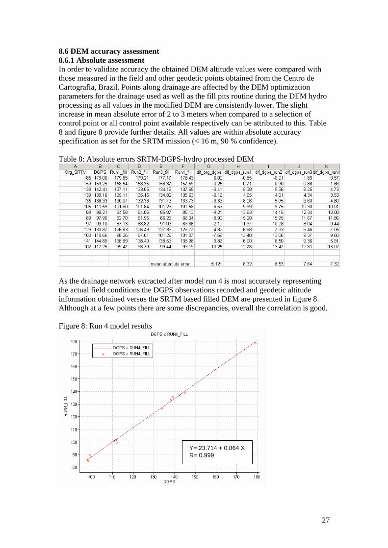
8.6 DEM accuracy assessment 8.6.1 Absolute assessment In order to validate accuracy the obtained DEM altitude values were compared with those measured in the field and other geodetic points obtained from the Centro de Cartografia, Brazil. Points along drainage are affected by the DEM optimization parameters for the drainage used as well as the fill pits routine during the DEM hydro processing as all values in the modified DEM are consistently lower. The slight increase in mean absolute error of 2 to 3 meters when compared to a selection of control point or all control point available respectively can be attributed to this. Table 8 and figure 8 provide further details. All values are within absolute accuracy specification as set for the SRTM mission (< 16 m, 90 % confidence). Table 8: Absolute errors SRTM-DGPS-hydro processed DEM

As the drainage network extracted after model run 4 is most accurately representing the actual field conditions the DGPS observations recorded and geodetic altitude information obtained versus the SRTM based filled DEM are presented in figure 8. Although at a few points there are some discrepancies, overall the correlation is good. Figure 8: Run 4 model results

Y= 23.714 + 0.864 XR= 0.999

28

8.6.2 Relative assessment As stated above the extracted main river network is a good indicator of the relative accuracy. Run 4 is fairly well representing the actual conditions as found during the field survey and is given in figure 9 using the Landsat-TM image as background. The drainage extraction method used does not allow incorporation of avulsions, therefore the Taquari does not continue at the Caronal avulsion. This still means that when this DEM is incorporated in a hydro-dynamic model part of the flow would continue to flow through the Taquari. Figure 9: Extracted drainage

This is shown by the DEM of the Caronal region given in figure 10. The arrows at locations B and C indicate the position of the Taquari river and other avulsions which is clearly visible by the deviating color (e.g. cyan continuing in light green) showing the lower elevated portions for the river. The active Caronal avulsion is indicated by A. The black drainage lines indicate the extracted drainage, using a flow accumulation threshold of 4000 contributing pixels. Figure 10: DEM of the Caronal region

29

As the minor secondary drainage is not used in the optimization process, there are deviations with regard to this drainage type extracted when using smaller flow accumulation thresholds. It is thought that these local differences will not seriously affect the usage of the DEM for hydro-dynamic modeling. Another way to evaluate the relative DEM processing results is to compare the difference map with the satellite images. The difference map was generated subtracting the processed DEM from the original DEM. Figure 11 is showing the difference map and the corresponding satellite image window. Figure 11: DEM difference map and satellite image window

The difference map displayed in gray scale is overlaid using with the satellite image and a linear profile tool is used to evaluate the absolute difference obtained along a section shown is the upper right sub window. The differences represent the height of the different vegetation types as observed in the field and the corresponding locations can be validated from the satellite images, e.g. the bright green vegetation along the river on the image represents evergreen trees mostly higher than 5 meters. The darker purple areas represent open areas which are scarcely vegetated and hardly any corrections have been applied in these areas. The same procedure as indicated above can also be used to compare the satellite image with the processed DEM directly. Examples are given in figures 12 and 13. Figure 12 is clearly showing the effects of the drainage optimization used. The riverbed is approximately 2.5 to 3 m below the main terrain surface. The areas adjacent the Taquari river and Caronal avulsion are showing minor relief differences and even a shallow depression representing an infilled backswamp along the levee. Figure 13 is showing a 20 km long section, from the uplands (south-east of Corumba) into the Paraguay floodplain. The higher elevated Paraguay levees are the prominent elevated portions; the remaining areas are flat, showing local incisions when crossing minor drainage lines.

30

Figure 12: Processed DEM and satellite image window Caronal avulsion

Figure 13: Processed DEM and satellite image window Paraguay floodplain

A final relative assessment conducted was reclassification of the difference map into elevation difference classes and draping these over the satellite image. These difference classes are representative of a number of prominent vegetation types occurring in the region like forest, bushes – shrubs – other herbaceous vegetation and reed – grass – water hyacinth. An example is provided in figure 14. As can be seen the levees along the Taquari as well as the fossil and secondary levees show a another difference class expressing the relationship between slightly higher elevated terrain portions and their influence on the occurrence of evergreen tree species. In the backswamps hardly any height difference is computed, showing the minimal correction applied to reed and water hyacinth and no corrections at all in the case of open water bodies. The correction applied reflects the main morphology of the terrain and the relationship with the occurrence of vegetation. This fact could also be observed in the Paraguay floodplain.

31

Figure 14: Spatial distribution of elevation differences computed

Figure 15 is showing the final DEM. The correction applied to incorporate the bathymetry is clearly visible. The DEM is visualized using a strong vertical exaggeration. Figure 15: The Final DEM obtained

32

9 Conclusions From this work presented a number of conclusions may be drawn with regard to the the first main problem stated in the introduction, namely: the development of a river flow and sedimentation model of the lower Taquari in the Pantanal. The model requires a good representation of the terrain. The effort presented here is reflecting this need. From the activities and analysis conducted additional conclusions can be made.

1. To cover the whole Pantanal region with laser scanning is not feasible. The only contribution that laser scanning could make is to further validate the DEM processing results conducted in this study. Laser scanning could be an option when a small area, like the Caronal avulsion, has to be studied in detail. This would also require adequate hydro-sedimentological data, which at the moment are not available, in order to successfully apply these dynamic models. Laser scanning is an operational technique in Brazil and three organizations are capable of doing the scanning and processing.

2. The field survey conducted provided a lot of additional information needed to perform the activities as given in this report. All data recorded could be successfully retrieved, (post) processed and integrated into a geographic information system to compare to available satellite images. As the area is very large and inaccessible the field observations made along the Taquari river are extrapolated to other regions in order to validate the DEM processing results. More fieldwork for a better assessment is needed.

3. The SRTM elevation model developed could also be used as an absolute model. The overall absolute vertical accuracy obtained is in the order of 5 to 10 meters, larger deviations occur in the Paraguay floodplain, most likely caused by finishing algorithms applied by the data provider. To overcome this problem the regression results presented (figure 8) could be adopted to get a more accurate altitude representation of this area. The absolute error is within the accuracy specifications given by the data provider

4. Several model runs are conducted. Run 4 represents the current diversion of discharge at the active Caronal avulsion and is regarded the best DEM.

5. The DEM optimization parameters used are realistic for the different drainage types in the Pantanal. Parameters B and C have been selected based on the sounding data collected and the width of the rivers (A) was measured directly from the satellite images and compared to the track records of the survey. Even after the fill pit routine (in the DEM hydro-processing stage) the river depth is realistic

6. The DEM processing could be successfully conducted using the process of hierarchic robust interpolation. The vegetation in the Pantanal region could be removed. The different runs conducted show deviating results with regard to the main drainage extracted, representing the importance of the Caronal avulsion area. Slight modifications have main implications over here. The parameters adopted in the filtering and interpolation routines are “over-removing” vegetation from the hills and the mountains bordering the Pantanal region. These areas should not be considered realistic.

7. The difference map produced (original SRTM_DEM – Processed_DEM) shows a good relationship with the different main vegetation type heights as found during the field survey. Also the morphology is fairly well represented.

33

As was described before, the Taquari river is traversing three distinct main landscape units and the avulsion areas are occurring in the gradual transition zones between these main landscape units: the Caronal avulsion is found in between the upper and the middle zone and the Ze Da Costa marks the transition between the middle and lower zone. The differences in longitudinal profile in these zones should be measured more extensively before more conclusive statements can be made but given collected DGPS measurements small changes in slope do exist. A reason for this change in slope near the Caronal avulsion might be due to (neo) tectonic influences as the lineaments could be identified crossing the Pantanal from the North-east to the South-west. At the place where the lineaments are crossing the Taquari the river pattern starts changing as well. Overall a large amount of data was collected. A backup is made at ITC and is available to the project team members. The most relevant data – processing results was already provided to Alterra to be incorporated for other analysis.

34

References Below web based references are given of resources used during this project. Processing software used: ARCVIEW – HEC-GeoHMS: http://www.hec.usace.army.mil ARCGIS: - Hydrotools: http://www.ce.utexas.edu/prof/maidment/grad/whiteaker/hydrotools.html - Taudem: http://emrc.usu.edu/software/htmlhelp/mw_help/tau.htm DiGeM: http://www.geogr.uni-goettingen.de/pg/saga/digem/index.html ILWIS: http://www.itc.nl/ilwis/ SCOP++, Inpho: http://www.inpho.de/scop.htm Data Archives: Geo data warehouse ITC: http://geodata.itc.nl Landsat: http://glcf.umiacs.umd.edu/aboutUs/ http://esip.umiacs.umd.edu/data/ ftp://ftp.glcf.umiacs.umd.edu/glcf/Landsat/WRS2/ Landsat, Aster, Modis: http://glovis.usgs.gov http://edcimswww.cr.usgs.gov/pub/imswelcome/ SRTM C-Band: http://srtm.usgs.gov/ and http://seamless.usgs.gov/ X-Band: http://www.caf.dlr.de/SRTM/SRTM_en.html JERS: http://southport.jpl.nasa.gov/grfm/ and http://www.eorc.nasda.go.jp/jers-1 Lidar companies, institutes and literature: Esteio : http://www.esteio.com.br/ Geoid : http://www.geoid.com.br LACTEC : http://www.lactec.org.br Optech ALTM : http://www.optech.on.ca/links.htm/ TopScan : http://www.topscan.de/en/index.php Loch, R.E.N. and Schäfer, A.G. (2004): Airborne laser scanning in the Brazilian market. Paper presented in Commission 6, ISPRS 2004, Istanbul, Turkey. Available at: http://www.isprs.org/istanbul2004/comm6/papers/675.pdf DGPS: SCOUT –SOPAC: http://sopac.ucsd.edu/cgi-bin/SCOUT.cgi Leica SR530: http://www.leica-geosystems.com/gps/product/sr530.htm Leica Ski-Pro: http://www.leica-geosystems.com/gps/product/ski-pro.htm

35

Other DGPS (Dual Frequency) post processing facilities: Auto-Gipsy: http://milhouse.jpl.nasa.gov.ag/ OPUS: http://www.ngs.noaa.gov/OPUS/ AUSPOS: http://www.ga.gov.au/nmd/geodesy/sgc/wwwgps/ Sounder for bathymetric surveys: Fishfinder: http://www.garmin.com/marine Gartrip: http://www.gartrip.de

Arcview project The data processing results have been prepared into an arcview project to easily integrate with the other project partners activities. Details to transfer the files from CD to hard-disk are provided below:

1. Copy the directory /PforWP_Pantanal/ containing all the data onto your D drive

2. Start ARCVIEW and open an existing project, press OK 3. Go to the directory: D:/PforWP_Pantanal and select: Taquari_Pantanal as the

project to be opened 4. The whole content of the project will be loaded

Remarks: The Landsat TM image mosaic used is resampled to a spatial resolution of 180 meters (the images were acquired from 1998 to 2000). This was done so that the data would fit on CD. The SAC-C data is given in the original resolution; the file name shows the acquisition date. All spectral bands have been included so that another band combination can be selected. The Ze Da Costa and Caronal avulsions are included as depicted from aerial photographs as of 1960. An uncontrolled photo mosaic is given but the geometric accuracy is acceptable. The sub directory /Org_sounding/ is containing all of the original sounding data collected but these are not uploaded in the Taquari_Pantanal project file. If required this can be done by the user itself (using the Add Theme option). The sounding points of the Taquari and within the Caronal avulsion are merged within the files Ptaquari.shp and Pcaronal.shp respectively. In the attribute table a column Depth + 30 cm is given meaning that 30 cm should still be added to the depth as given in this column to obtain the real river depth recorded at the moment of survey (30 March-04 April 2004). The shape file sounderpoints.shp is given a column sourcetheme, showing the source files for the selected points. The altitude information in these sounder point attribute tables was collected using a GPS 72, no post processing was applied. Therefore these measurements are not very accurate (in the order of >10 m.) The Lcaronal.shp and the Ltaquari.shp provide the merged track records. Again in the sub directory /Org_sounding/ the original data is provided. The Dem_SRTMorg is the original SRTM data, the DEM-New is the processed DEM. The difference between the two is the Veg_height theme, which is reclassified into a number of elevation classes. The Themes Carlos_..... are recorded by Embrapa and provide additional descriptions in the attribute tables.

Problems during starting of the project are encountered when certain extensions are not available. For this project use has been made of the following extensions:

• 3D Analyst • IMAGINE Image Support • Spatial Analyst

If these extensions are available they are loaded automatically.

APPENDIX 1.

REMOTE SENSING IMAGE ANALYSIS AND ALTITUDE DETERMINATION OF THE RIO TAQUARI – PANTANAL SYSTEM

APPENDIX 2.

SRTM – DERIVED DEM: OPTIMIZATION FOR HYDROLOGIC MODELING

APPENDIX 3.

PANTANAL DIGITAL TERRAIN MODEL.

APPENDIX 4:

DEM PROCESSING MODEL RUNS 1 – 4

FULL DETAILS

DEM PROCESSING: RUN-1 ----------------------------------------------------------------------- ThinOut VERS 5.2.2 step nb.0 04May 04 19:59:23 ----------------------------------------------------------------------- Input: d:\dem_scop\pant\run1\run1_.all Output: d:\dem_scop\pant\run1\step0.tho Cell size: 450.000 Method: Mean Area: Left lower corner: 420911.000 7868468.000 Size: 320220.000 149130.000 Nb of input points: 5900822 Nb of output points: 236384 END SCOP.ThinOut ----------------------------------------------------------------------- Filter step nb.1 04May 04 20:03:11 ----------------------------------------------------------------------- Input: d:\dem_scop\pant\run1\step0.tho DTM: d:\dem_scop\pant\run1\step1.dtm Output ground: d:\dem_scop\pant\run1\step1.grd Output vegetation: d:\dem_scop\pant\run1\step1.veg DIGITAL ELEVATION MODEL MAP SHEET POSITION AND SIZE LEFT LOWER CORNER EAST .......... 420911.00 NORTH .......... 7868468.00 EXTENSION EAST .......... 320220.00 NORTH .......... 149130.00 CHARACTERISTICS OF THE DEM GRID WIDTH EAST ......... 450.00 NORTH ......... 450.00 NUMBER OF GRID LINES EAST ......... 13 NORTH ......... 13 NUMBER OF INTERPOLATED COMPUTING UNITS .... 1680 NUMBER OF STORED GRID POINTS ......... 283920 NUMBER OF GRID INTERSECTIONS ......... 0 INFORMATION ABOUT THE INTERPOLATION LINEAR PREDICTION NUMBER OF REFERENCE POINTS GIVEN .......... 236384 SINGLE POINTS ........... 236384 HIGHS AND LOWS ........... 0 LINE POINTS ........... 0 AVERAGE FILTER VALUES SINGLE POINTS ........... 2.366 HIGHS AND LOWS ........... .000 LINE POINTS ........... .000 MAXIMUM FILTER VALUES SINGLE POINTS ........... 115.262

HIGHS AND LOWS ........... .000 LINE POINTS ........... .000 ----------------------------------------------------------------------- Filter step nb.2 04May 04 20:04:27 ----------------------------------------------------------------------- Input: d:\dem_scop\pant\run1\step1.grd DTM: d:\dem_scop\pant\run1\step2.dtm Output ground: d:\dem_scop\pant\run1\step2.grd Output vegetation: d:\dem_scop\pant\run1\step2.veg DIGITAL ELEVATION MODEL MAP SHEET POSITION AND SIZE LEFT LOWER CORNER EAST .......... 420911.00 NORTH .......... 7868468.00 EXTENSION EAST .......... 320220.00 NORTH .......... 149130.00 CHARACTERISTICS OF THE DEM GRID WIDTH EAST ......... 450.00 NORTH ......... 450.00 NUMBER OF GRID LINES EAST ......... 11 NORTH ......... 11 NUMBER OF INTERPOLATED COMPUTING UNITS .... 2447 NUMBER OF STORED GRID POINTS ......... 296087 NUMBER OF GRID INTERSECTIONS ......... 0 INFORMATION ABOUT THE INTERPOLATION LINEAR PREDICTION NUMBER OF REFERENCE POINTS GIVEN .......... 196221 SINGLE POINTS ........... 196221 HIGHS AND LOWS ........... 0 LINE POINTS ........... 0 AVERAGE FILTER VALUES SINGLE POINTS ........... .539 HIGHS AND LOWS ........... .000 LINE POINTS ........... .000 MAXIMUM FILTER VALUES SINGLE POINTS ........... 5.652 HIGHS AND LOWS ........... .000 LINE POINTS ........... .000 ----------------------------------------------------------------------- Interpolation step nb.3 04May 04 20:04:52 ----------------------------------------------------------------------- Input: d:\dem_scop\pant\run1\step2.grd DTM: d:\dem_scop\pant\run1\step3.dtm DIGITAL ELEVATION MODEL MAP SHEET

POSITION AND SIZE LEFT LOWER CORNER EAST .......... 420911.00 NORTH .......... 7868468.00 EXTENSION EAST .......... 320220.00 NORTH .......... 149130.00 CHARACTERISTICS OF THE DEM GRID WIDTH EAST ......... 150.00 NORTH ......... 150.00 NUMBER OF GRID LINES EAST ......... 11 NORTH ......... 11 NUMBER OF INTERPOLATED COMPUTING UNITS .... 21382 NUMBER OF STORED GRID POINTS ......... 2587222 NUMBER OF GRID INTERSECTIONS ......... 0 INFORMATION ABOUT THE INTERPOLATION LINEAR PREDICTION NUMBER OF REFERENCE POINTS GIVEN .......... 101126 SINGLE POINTS ........... 101126 HIGHS AND LOWS ........... 0 LINE POINTS ........... 0 AVERAGE FILTER VALUES SINGLE POINTS ........... .284 HIGHS AND LOWS ........... .000 LINE POINTS ........... .000 MAXIMUM FILTER VALUES SINGLE POINTS ........... 2.287 HIGHS AND LOWS ........... .000 LINE POINTS ........... .000 ----------------------------------------------------------------------- SortOut VERS 5.2.2 step nb.4 04May 04 20:09:31 ----------------------------------------------------------------------- Input: d:\dem_scop\pant\run1\run1_.all DTM: d:\dem_scop\pant\run1\step3.dtm Output: d:\dem_scop\pant\run1\step4.sog Lower distance: -10.000 Upper distance: 2.500 Nb of input points: 5900822 Nb of output points: 4292648 END SCOP.SortOut ----------------------------------------------------------------------- ThinOut VERS 5.2.2 step nb.5 04May 04 20:11:30 ----------------------------------------------------------------------- Input: d:\dem_scop\pant\run1\step4.sog Output: d:\dem_scop\pant\run1\step5.tho Cell size: 210.000 Method: Mean Area: Left lower corner: 420911.000 7868468.000

Size: 320220.000 149130.000 Nb of input points: 4292648 Nb of output points: 936515 END SCOP.ThinOut ----------------------------------------------------------------------- Filter step nb.6 04May 04 20:27:57 ----------------------------------------------------------------------- Input: d:\dem_scop\pant\run1\step5.tho DTM: d:\dem_scop\pant\run1\step6.dtm Output ground: d:\dem_scop\pant\run1\step6.grd Output vegetation: d:\dem_scop\pant\run1\step6.veg DIGITAL ELEVATION MODEL MAP SHEET POSITION AND SIZE LEFT LOWER CORNER EAST .......... 420911.00 NORTH .......... 7868468.00 EXTENSION EAST .......... 320220.00 NORTH .......... 149130.00 CHARACTERISTICS OF THE DEM GRID WIDTH EAST ......... 210.00 NORTH ......... 210.00 NUMBER OF GRID LINES EAST ......... 16 NORTH ......... 16 NUMBER OF INTERPOLATED COMPUTING UNITS .... 4896 NUMBER OF STORED GRID POINTS ......... 1253376 NUMBER OF GRID INTERSECTIONS ......... 0 INFORMATION ABOUT THE INTERPOLATION LINEAR PREDICTION NUMBER OF REFERENCE POINTS GIVEN .......... 936515 SINGLE POINTS ........... 936515 HIGHS AND LOWS ........... 0 LINE POINTS ........... 0 AVERAGE FILTER VALUES SINGLE POINTS ........... .391 HIGHS AND LOWS ........... .000 LINE POINTS ........... .000 MAXIMUM FILTER VALUES SINGLE POINTS ........... 22.661 HIGHS AND LOWS ........... .000 LINE POINTS ........... .000 ----------------------------------------------------------------------- Interpolation step nb.7 04May 04 20:28:43 ----------------------------------------------------------------------- Input: d:\dem_scop\pant\run1\step6.grd DTM: d:\dem_scop\pant\run1\step7.dtm

DIGITAL ELEVATION MODEL MAP SHEET POSITION AND SIZE LEFT LOWER CORNER EAST .......... 420911.00 NORTH .......... 7868468.00 EXTENSION EAST .......... 320220.00 NORTH .......... 149130.00 CHARACTERISTICS OF THE DEM GRID WIDTH EAST ......... 90.00 NORTH ......... 90.00 NUMBER OF GRID LINES EAST ......... 16 NORTH ......... 16 NUMBER OF INTERPOLATED COMPUTING UNITS .... 26373 NUMBER OF STORED GRID POINTS ......... 6751488 NUMBER OF GRID INTERSECTIONS ......... 0 INFORMATION ABOUT THE INTERPOLATION LINEAR PREDICTION NUMBER OF REFERENCE POINTS GIVEN .......... 262053 SINGLE POINTS ........... 262053 HIGHS AND LOWS ........... 0 LINE POINTS ........... 0 AVERAGE FILTER VALUES SINGLE POINTS ........... .285 HIGHS AND LOWS ........... .000 LINE POINTS ........... .000 MAXIMUM FILTER VALUES SINGLE POINTS ........... 5.119 HIGHS AND LOWS ........... .000 LINE POINTS ........... .000 ----------------------------------------------------------------------- SortOut VERS 5.2.2 step nb.8 04May 04 20:33:27 ----------------------------------------------------------------------- Input: d:\dem_scop\pant\run1\run1_.all DTM: d:\dem_scop\pant\run1\step7.dtm Output: d:\dem_scop\pant\run1\step8.sog Lower distance: -3.000 Upper distance: 1.500 Nb of input points: 5900822 Nb of output points: 3005105 END SCOP.SortOut ----------------------------------------------------------------------- Filter step nb.9 04May 04 20:54:51 ----------------------------------------------------------------------- Input: d:\dem_scop\pant\run1\step8.sog DTM: d:\dem_scop\pant\run1\step9.dtm Output ground: d:\dem_scop\pant\run1\step9.grd Output vegetation: d:\dem_scop\pant\run1\step9.veg

DIGITAL ELEVATION MODEL MAP SHEET POSITION AND SIZE LEFT LOWER CORNER EAST .......... 420911.00 NORTH .......... 7868468.00 EXTENSION EAST .......... 320220.00 NORTH .......... 149130.00 CHARACTERISTICS OF THE DEM GRID WIDTH EAST ......... 90.00 NORTH ......... 90.00 NUMBER OF GRID LINES EAST ......... 16 NORTH ......... 16 NUMBER OF INTERPOLATED COMPUTING UNITS .... 26380 NUMBER OF STORED GRID POINTS ......... 6753280 NUMBER OF GRID INTERSECTIONS ......... 0 INFORMATION ABOUT THE INTERPOLATION LINEAR PREDICTION NUMBER OF REFERENCE POINTS GIVEN .......... 3005105 SINGLE POINTS ........... 3005105 HIGHS AND LOWS ........... 0 LINE POINTS ........... 0 AVERAGE FILTER VALUES SINGLE POINTS ........... .430 HIGHS AND LOWS ........... .000 LINE POINTS ........... .000 MAXIMUM FILTER VALUES SINGLE POINTS ........... 33.926 HIGHS AND LOWS ........... .000 LINE POINTS ........... .000 ----------------------------------------------------------------------- Interpolation step nb.10 04May 04 21:01:57 ----------------------------------------------------------------------- Input: d:\dem_scop\pant\run1\step9.grd DTM: d:\dem_scop\pant\run1\step10.dtm DIGITAL ELEVATION MODEL MAP SHEET POSITION AND SIZE LEFT LOWER CORNER EAST .......... 420911.00 NORTH .......... 7868468.00 EXTENSION EAST .......... 320220.00 NORTH .......... 149130.00 CHARACTERISTICS OF THE DEM GRID WIDTH EAST ......... 90.00 NORTH ......... 90.00 NUMBER OF GRID LINES EAST ......... 11 NORTH ......... 11

NUMBER OF INTERPOLATED COMPUTING UNITS .... 58558 NUMBER OF STORED GRID POINTS ......... 7085518 NUMBER OF GRID INTERSECTIONS ......... 0 INFORMATION ABOUT THE INTERPOLATION LINEAR PREDICTION NUMBER OF REFERENCE POINTS GIVEN .......... 881658 SINGLE POINTS ........... 881658 HIGHS AND LOWS ........... 0 LINE POINTS ........... 0 AVERAGE FILTER VALUES SINGLE POINTS ........... .275 HIGHS AND LOWS ........... .000 LINE POINTS ........... .000 MAXIMUM FILTER VALUES SINGLE POINTS ........... 3.064 HIGHS AND LOWS ........... .000 LINE POINTS ........... .000

DEM PROCESSING: RUN-2 ----------------------------------------------------------------------- ThinOut VERS 5.2.2 step nb.0 04May 11 20:15:39 ----------------------------------------------------------------------- Input: d:\dem_scop\run2\run2\run2_.all Output: d:\dem_scop\run2\run2\step0.tho Cell size: 360.000 Method: Center Area: Left lower corner: 420911.000 7868468.000 Size: 320220.000 149130.000 Nb of input points: 5900822 Nb of output points: 369350 END SCOP.ThinOut ----------------------------------------------------------------------- Filter step nb.1 04May 11 20:20:52 ----------------------------------------------------------------------- Input: d:\dem_scop\run2\run2\step0.tho DTM: d:\dem_scop\run2\run2\step1.dtm Output ground: d:\dem_scop\run2\run2\step1.grd Output vegetation: d:\dem_scop\run2\run2\step1.veg DIGITAL ELEVATION MODEL MAP SHEET POSITION AND SIZE LEFT LOWER CORNER EAST .......... 420911.00 NORTH .......... 7868468.00 EXTENSION EAST .......... 320220.00 NORTH .......... 149130.00 CHARACTERISTICS OF THE DEM GRID WIDTH EAST ......... 360.00 NORTH ......... 360.00 NUMBER OF GRID LINES EAST ......... 13 NORTH ......... 13 NUMBER OF INTERPOLATED COMPUTING UNITS .... 2625 NUMBER OF STORED GRID POINTS ......... 443625 NUMBER OF GRID INTERSECTIONS ......... 0 INFORMATION ABOUT THE INTERPOLATION LINEAR PREDICTION NUMBER OF REFERENCE POINTS GIVEN .......... 369350 SINGLE POINTS ........... 369350 HIGHS AND LOWS ........... 0 LINE POINTS ........... 0 AVERAGE FILTER VALUES SINGLE POINTS ........... 2.775 HIGHS AND LOWS ........... .000 LINE POINTS ........... .000 MAXIMUM FILTER VALUES SINGLE POINTS ........... 146.173

HIGHS AND LOWS ........... .000 LINE POINTS ........... .000 ----------------------------------------------------------------------- Filter step nb.2 04May 11 20:22:03 ----------------------------------------------------------------------- Input: d:\dem_scop\run2\run2\step1.grd DTM: d:\dem_scop\run2\run2\step2.dtm Output ground: d:\dem_scop\run2\run2\step2.grd Output vegetation: d:\dem_scop\run2\run2\step2.veg DIGITAL ELEVATION MODEL MAP SHEET POSITION AND SIZE LEFT LOWER CORNER EAST .......... 420911.00 NORTH .......... 7868468.00 EXTENSION EAST .......... 320220.00 NORTH .......... 149130.00 CHARACTERISTICS OF THE DEM GRID WIDTH EAST ......... 360.00 NORTH ......... 360.00 NUMBER OF GRID LINES EAST ......... 11 NORTH ......... 11 NUMBER OF INTERPOLATED COMPUTING UNITS .... 3738 NUMBER OF STORED GRID POINTS ......... 452298 NUMBER OF GRID INTERSECTIONS ......... 0 INFORMATION ABOUT THE INTERPOLATION LINEAR PREDICTION NUMBER OF REFERENCE POINTS GIVEN .......... 256406 SINGLE POINTS ........... 256406 HIGHS AND LOWS ........... 0 LINE POINTS ........... 0 AVERAGE FILTER VALUES SINGLE POINTS ........... .782 HIGHS AND LOWS ........... .000 LINE POINTS ........... .000 MAXIMUM FILTER VALUES SINGLE POINTS ........... 11.119 HIGHS AND LOWS ........... .000 LINE POINTS ........... .000 ----------------------------------------------------------------------- Interpolation step nb.3 04May 11 20:22:37 ----------------------------------------------------------------------- Input: d:\dem_scop\run2\run2\step2.grd DTM: d:\dem_scop\run2\run2\step3.dtm DIGITAL ELEVATION MODEL

MAP SHEET POSITION AND SIZE LEFT LOWER CORNER EAST .......... 420911.00 NORTH .......... 7868468.00 EXTENSION EAST .......... 320220.00 NORTH .......... 149130.00 CHARACTERISTICS OF THE DEM GRID WIDTH EAST ......... 90.00 NORTH ......... 90.00 NUMBER OF GRID LINES EAST ......... 11 NORTH ......... 11 NUMBER OF INTERPOLATED COMPUTING UNITS .... 58898 NUMBER OF STORED GRID POINTS ......... 7126658 NUMBER OF GRID INTERSECTIONS ......... 0 INFORMATION ABOUT THE INTERPOLATION LINEAR PREDICTION NUMBER OF REFERENCE POINTS GIVEN .......... 83038 SINGLE POINTS ........... 83038 HIGHS AND LOWS ........... 0 LINE POINTS ........... 0 AVERAGE FILTER VALUES SINGLE POINTS ........... .394 HIGHS AND LOWS ........... .000 LINE POINTS ........... .000 MAXIMUM FILTER VALUES SINGLE POINTS ........... 2.930 HIGHS AND LOWS ........... .000 LINE POINTS ........... .000 ----------------------------------------------------------------------- SortOut VERS 5.2.2 step nb.4 04May 11 20:27:22 ----------------------------------------------------------------------- Input: d:\dem_scop\run2\run2\run2_.all DTM: d:\dem_scop\run2\run2\step3.dtm Output: d:\dem_scop\run2\run2\step4.sog Lower distance: -10.000 Upper distance: 2.500 Nb of input points: 5900822 Nb of output points: 3293098 END SCOP.SortOut ----------------------------------------------------------------------- ThinOut VERS 5.2.2 step nb.5 04May 11 20:29:01 ----------------------------------------------------------------------- Input: d:\dem_scop\run2\run2\step4.sog Output: d:\dem_scop\run2\run2\step5.tho Cell size: 180.000 Method: Mean Area:

Left lower corner: 420911.000 7868468.000 Size: 320220.000 149130.000 Nb of input points: 3293098 Nb of output points: 1082521 END SCOP.ThinOut ----------------------------------------------------------------------- Filter step nb.6 04May 11 20:39:51 ----------------------------------------------------------------------- Input: d:\dem_scop\run2\run2\step5.tho DTM: d:\dem_scop\run2\run2\step6.dtm Output ground: d:\dem_scop\run2\run2\step6.grd Output vegetation: d:\dem_scop\run2\run2\step6.veg DIGITAL ELEVATION MODEL MAP SHEET POSITION AND SIZE LEFT LOWER CORNER EAST .......... 420911.00 NORTH .......... 7868468.00 EXTENSION EAST .......... 320220.00 NORTH .......... 149130.00 CHARACTERISTICS OF THE DEM GRID WIDTH EAST ......... 180.00 NORTH ......... 180.00 NUMBER OF GRID LINES EAST ......... 16 NORTH ......... 16 NUMBER OF INTERPOLATED COMPUTING UNITS .... 6664 NUMBER OF STORED GRID POINTS ......... 1705984 NUMBER OF GRID INTERSECTIONS ......... 0 INFORMATION ABOUT THE INTERPOLATION LINEAR PREDICTION NUMBER OF REFERENCE POINTS GIVEN .......... 1082521 SINGLE POINTS ........... 1082521 HIGHS AND LOWS ........... 0 LINE POINTS ........... 0 AVERAGE FILTER VALUES SINGLE POINTS ........... .369 HIGHS AND LOWS ........... .000 LINE POINTS ........... .000 MAXIMUM FILTER VALUES SINGLE POINTS ........... 7.381 HIGHS AND LOWS ........... .000 LINE POINTS ........... .000 ----------------------------------------------------------------------- Interpolation step nb.7 04May 11 20:40:36 ----------------------------------------------------------------------- Input: d:\dem_scop\run2\run2\step6.grd DTM: d:\dem_scop\run2\run2\step7.dtm

DIGITAL ELEVATION MODEL MAP SHEET POSITION AND SIZE LEFT LOWER CORNER EAST .......... 420911.00 NORTH .......... 7868468.00 EXTENSION EAST .......... 320220.00 NORTH .......... 149130.00 CHARACTERISTICS OF THE DEM GRID WIDTH EAST ......... 90.00 NORTH ......... 90.00 NUMBER OF GRID LINES EAST ......... 16 NORTH ......... 16 NUMBER OF INTERPOLATED COMPUTING UNITS .... 26382 NUMBER OF STORED GRID POINTS ......... 6753792 NUMBER OF GRID INTERSECTIONS ......... 0 INFORMATION ABOUT THE INTERPOLATION LINEAR PREDICTION NUMBER OF REFERENCE POINTS GIVEN .......... 301551 SINGLE POINTS ........... 301551 HIGHS AND LOWS ........... 0 LINE POINTS ........... 0 AVERAGE FILTER VALUES SINGLE POINTS ........... .259 HIGHS AND LOWS ........... .000 LINE POINTS ........... .000 MAXIMUM FILTER VALUES SINGLE POINTS ........... 4.004 HIGHS AND LOWS ........... .000 LINE POINTS ........... .000 ----------------------------------------------------------------------- SortOut VERS 5.2.2 step nb.8 04May 11 20:45:20 ----------------------------------------------------------------------- Input: d:\dem_scop\run2\run2\run2_.all DTM: d:\dem_scop\run2\run2\step7.dtm Output: d:\dem_scop\run2\run2\step8.sog Lower distance: -3.000 Upper distance: 1.500 Nb of input points: 5900822 Nb of output points: 2546716 END SCOP.SortOut ----------------------------------------------------------------------- Filter step nb.9 04May 11 21:05:40 ----------------------------------------------------------------------- Input: d:\dem_scop\run2\run2\step8.sog DTM: d:\dem_scop\run2\run2\step9.dtm Output ground: d:\dem_scop\run2\run2\step9.grd Output vegetation: d:\dem_scop\run2\run2\step9.veg

DIGITAL ELEVATION MODEL MAP SHEET POSITION AND SIZE LEFT LOWER CORNER EAST .......... 420911.00 NORTH .......... 7868468.00 EXTENSION EAST .......... 320220.00 NORTH .......... 149130.00 CHARACTERISTICS OF THE DEM GRID WIDTH EAST ......... 90.00 NORTH ......... 90.00 NUMBER OF GRID LINES EAST ......... 16 NORTH ......... 16 NUMBER OF INTERPOLATED COMPUTING UNITS .... 26382 NUMBER OF STORED GRID POINTS ......... 6753792 NUMBER OF GRID INTERSECTIONS ......... 0 INFORMATION ABOUT THE INTERPOLATION LINEAR PREDICTION NUMBER OF REFERENCE POINTS GIVEN .......... 2546716 SINGLE POINTS ........... 2546716 HIGHS AND LOWS ........... 0 LINE POINTS ........... 0 AVERAGE FILTER VALUES SINGLE POINTS ........... .413 HIGHS AND LOWS ........... .000 LINE POINTS ........... .000 MAXIMUM FILTER VALUES SINGLE POINTS ........... 12.893 HIGHS AND LOWS ........... .000 LINE POINTS ........... .000 ----------------------------------------------------------------------- Interpolation step nb.10 04May 11 21:07:00 ----------------------------------------------------------------------- Input: d:\dem_scop\run2\run2\step9.grd DTM: d:\dem_scop\run2\run2\step10.dtm DIGITAL ELEVATION MODEL MAP SHEET POSITION AND SIZE LEFT LOWER CORNER EAST .......... 420911.00 NORTH .......... 7868468.00 EXTENSION EAST .......... 320220.00 NORTH .......... 149130.00 CHARACTERISTICS OF THE DEM GRID WIDTH EAST ......... 90.00 NORTH ......... 90.00 NUMBER OF GRID LINES EAST ......... 11 NORTH ......... 11

NUMBER OF INTERPOLATED COMPUTING UNITS .... 58708 NUMBER OF STORED GRID POINTS ......... 7103668 NUMBER OF GRID INTERSECTIONS ......... 0 INFORMATION ABOUT THE INTERPOLATION LINEAR PREDICTION NUMBER OF REFERENCE POINTS GIVEN .......... 783371 SINGLE POINTS ........... 783371 HIGHS AND LOWS ........... 0 LINE POINTS ........... 0 AVERAGE FILTER VALUES SINGLE POINTS ........... .275 HIGHS AND LOWS ........... .000 LINE POINTS ........... .000 MAXIMUM FILTER VALUES SINGLE POINTS ........... 3.692 HIGHS AND LOWS ........... .000 LINE POINTS ........... .000

DEM PROCESSING: RUN- 3 ----------------------------------------------------------------------- ThinOut VERS 5.2.2 step nb.0 04May 12 10:15:46 ----------------------------------------------------------------------- Input: d:\dem_scop\run3\run3\run3_.all Output: d:\dem_scop\run3\run3\step0.tho Cell size: 360.000 Method: Mean Area: Left lower corner: 420911.000 7868468.000 Size: 320220.000 149130.000 Nb of input points: 5900822 Nb of output points: 369350 END SCOP.ThinOut ----------------------------------------------------------------------- Filter step nb.1 04May 12 10:21:36 ----------------------------------------------------------------------- Input: d:\dem_scop\run3\run3\step0.tho DTM: d:\dem_scop\run3\run3\step1.dtm Output ground: d:\dem_scop\run3\run3\step1.grd Output vegetation: d:\dem_scop\run3\run3\step1.veg DIGITAL ELEVATION MODEL MAP SHEET POSITION AND SIZE LEFT LOWER CORNER EAST .......... 420911.00 NORTH .......... 7868468.00 EXTENSION EAST .......... 320220.00 NORTH .......... 149130.00 CHARACTERISTICS OF THE DEM GRID WIDTH EAST ......... 360.00 NORTH ......... 360.00 NUMBER OF GRID LINES EAST ......... 13 NORTH ......... 13 NUMBER OF INTERPOLATED COMPUTING UNITS .... 2625 NUMBER OF STORED GRID POINTS ......... 443625 NUMBER OF GRID INTERSECTIONS ......... 0 INFORMATION ABOUT THE INTERPOLATION LINEAR PREDICTION NUMBER OF REFERENCE POINTS GIVEN .......... 369350 SINGLE POINTS ........... 369350 HIGHS AND LOWS ........... 0 LINE POINTS ........... 0 AVERAGE FILTER VALUES SINGLE POINTS ........... 2.162 HIGHS AND LOWS ........... .000 LINE POINTS ........... .000 MAXIMUM FILTER VALUES SINGLE POINTS ........... 127.574

HIGHS AND LOWS ........... .000 LINE POINTS ........... .000 ----------------------------------------------------------------------- Filter step nb.2 04May 12 10:23:27 ----------------------------------------------------------------------- Input: d:\dem_scop\run3\run3\step1.grd DTM: d:\dem_scop\run3\run3\step2.dtm Output ground: d:\dem_scop\run3\run3\step2.grd Output vegetation: d:\dem_scop\run3\run3\step2.veg DIGITAL ELEVATION MODEL MAP SHEET POSITION AND SIZE LEFT LOWER CORNER EAST .......... 420911.00 NORTH .......... 7868468.00 EXTENSION EAST .......... 320220.00 NORTH .......... 149130.00 CHARACTERISTICS OF THE DEM GRID WIDTH EAST ......... 360.00 NORTH ......... 360.00 NUMBER OF GRID LINES EAST ......... 11 NORTH ......... 11 NUMBER OF INTERPOLATED COMPUTING UNITS .... 3738 NUMBER OF STORED GRID POINTS ......... 452298 NUMBER OF GRID INTERSECTIONS ......... 0 INFORMATION ABOUT THE INTERPOLATION LINEAR PREDICTION NUMBER OF REFERENCE POINTS GIVEN .......... 305688 SINGLE POINTS ........... 305688 HIGHS AND LOWS ........... 0 LINE POINTS ........... 0 AVERAGE FILTER VALUES SINGLE POINTS ........... .559 HIGHS AND LOWS ........... .000 LINE POINTS ........... .000 MAXIMUM FILTER VALUES SINGLE POINTS ........... 6.047 HIGHS AND LOWS ........... .000 LINE POINTS ........... .000 ----------------------------------------------------------------------- Interpolation step nb.3 04May 12 10:25:38 ----------------------------------------------------------------------- Input: d:\dem_scop\run3\run3\step2.grd DTM: d:\dem_scop\run3\run3\step3.dtm DIGITAL ELEVATION MODEL MAP SHEET

POSITION AND SIZE LEFT LOWER CORNER EAST .......... 420911.00 NORTH .......... 7868468.00 EXTENSION EAST .......... 320220.00 NORTH .......... 149130.00 CHARACTERISTICS OF THE DEM GRID WIDTH EAST ......... 90.00 NORTH ......... 90.00 NUMBER OF GRID LINES EAST ......... 11 NORTH ......... 11 NUMBER OF INTERPOLATED COMPUTING UNITS .... 59005 NUMBER OF STORED GRID POINTS ......... 7139605 NUMBER OF GRID INTERSECTIONS ......... 0 INFORMATION ABOUT THE INTERPOLATION LINEAR PREDICTION NUMBER OF REFERENCE POINTS GIVEN .......... 152874 SINGLE POINTS ........... 152874 HIGHS AND LOWS ........... 0 LINE POINTS ........... 0 AVERAGE FILTER VALUES SINGLE POINTS ........... .300 HIGHS AND LOWS ........... .000 LINE POINTS ........... .000 MAXIMUM FILTER VALUES SINGLE POINTS ........... 3.100 HIGHS AND LOWS ........... .000 LINE POINTS ........... .000 ----------------------------------------------------------------------- SortOut VERS 5.2.2 step nb.4 04May 12 10:30:21 ----------------------------------------------------------------------- Input: d:\dem_scop\run3\run3\run3_.all DTM: d:\dem_scop\run3\run3\step3.dtm Output: d:\dem_scop\run3\run3\step4.sog Lower distance: -10.000 Upper distance: 2.500 Nb of input points: 5900822 Nb of output points: 4290422 END SCOP.SortOut ----------------------------------------------------------------------- ThinOut VERS 5.2.2 step nb.5 04May 12 10:32:26 ----------------------------------------------------------------------- Input: d:\dem_scop\run3\run3\step4.sog Output: d:\dem_scop\run3\run3\step5.tho Cell size: 180.000 Method: Lowest Area: Left lower corner: 420911.000 7868468.000

Size: 320220.000 149130.000 Nb of input points: 4290422 Nb of output points: 1254129 END SCOP.ThinOut ----------------------------------------------------------------------- Filter step nb.6 04May 12 10:51:58 ----------------------------------------------------------------------- Input: d:\dem_scop\run3\run3\step5.tho DTM: d:\dem_scop\run3\run3\step6.dtm Output ground: d:\dem_scop\run3\run3\step6.grd Output vegetation: d:\dem_scop\run3\run3\step6.veg DIGITAL ELEVATION MODEL MAP SHEET POSITION AND SIZE LEFT LOWER CORNER EAST .......... 420911.00 NORTH .......... 7868468.00 EXTENSION EAST .......... 320220.00 NORTH .......... 149130.00 CHARACTERISTICS OF THE DEM GRID WIDTH EAST ......... 180.00 NORTH ......... 180.00 NUMBER OF GRID LINES EAST ......... 16 NORTH ......... 16 NUMBER OF INTERPOLATED COMPUTING UNITS .... 6664 NUMBER OF STORED GRID POINTS ......... 1705984 NUMBER OF GRID INTERSECTIONS ......... 0 INFORMATION ABOUT THE INTERPOLATION LINEAR PREDICTION NUMBER OF REFERENCE POINTS GIVEN .......... 1254129 SINGLE POINTS ........... 1254129 HIGHS AND LOWS ........... 0 LINE POINTS ........... 0 AVERAGE FILTER VALUES SINGLE POINTS ........... .380 HIGHS AND LOWS ........... .000 LINE POINTS ........... .000 MAXIMUM FILTER VALUES SINGLE POINTS ........... 24.675 HIGHS AND LOWS ........... .000 LINE POINTS ........... .000 ----------------------------------------------------------------------- Interpolation step nb.7 04May 12 10:53:12 ----------------------------------------------------------------------- Input: d:\dem_scop\run3\run3\step6.grd DTM: d:\dem_scop\run3\run3\step7.dtm

DIGITAL ELEVATION MODEL MAP SHEET POSITION AND SIZE LEFT LOWER CORNER EAST .......... 420911.00 NORTH .......... 7868468.00 EXTENSION EAST .......... 320220.00 NORTH .......... 149130.00 CHARACTERISTICS OF THE DEM GRID WIDTH EAST ......... 90.00 NORTH ......... 90.00 NUMBER OF GRID LINES EAST ......... 16 NORTH ......... 16 NUMBER OF INTERPOLATED COMPUTING UNITS .... 26405 NUMBER OF STORED GRID POINTS ......... 6759680 NUMBER OF GRID INTERSECTIONS ......... 0 INFORMATION ABOUT THE INTERPOLATION LINEAR PREDICTION NUMBER OF REFERENCE POINTS GIVEN .......... 402422 SINGLE POINTS ........... 402422 HIGHS AND LOWS ........... 0 LINE POINTS ........... 0 AVERAGE FILTER VALUES SINGLE POINTS ........... .290 HIGHS AND LOWS ........... .000 LINE POINTS ........... .000 MAXIMUM FILTER VALUES SINGLE POINTS ........... 5.018 HIGHS AND LOWS ........... .000 LINE POINTS ........... .000 ----------------------------------------------------------------------- SortOut VERS 5.2.2 step nb.8 04May 12 10:57:56 ----------------------------------------------------------------------- Input: d:\dem_scop\run3\run3\run3_.all DTM: d:\dem_scop\run3\run3\step7.dtm Output: d:\dem_scop\run3\run3\step8.sog Lower distance: -3.000 Upper distance: 1.500 Nb of input points: 5900822 Nb of output points: 1778819 END SCOP.SortOut ----------------------------------------------------------------------- Filter step nb.9 04May 12 11:08:27 ----------------------------------------------------------------------- Input: d:\dem_scop\run3\run3\step8.sog DTM: d:\dem_scop\run3\run3\step9.dtm Output ground: d:\dem_scop\run3\run3\step9.grd Output vegetation: d:\dem_scop\run3\run3\step9.veg

DIGITAL ELEVATION MODEL MAP SHEET POSITION AND SIZE LEFT LOWER CORNER EAST .......... 420911.00 NORTH .......... 7868468.00 EXTENSION EAST .......... 320220.00 NORTH .......... 149130.00 CHARACTERISTICS OF THE DEM GRID WIDTH EAST ......... 90.00 NORTH ......... 90.00 NUMBER OF GRID LINES EAST ......... 16 NORTH ......... 16 NUMBER OF INTERPOLATED COMPUTING UNITS .... 26407 NUMBER OF STORED GRID POINTS ......... 6760192 NUMBER OF GRID INTERSECTIONS ......... 0 INFORMATION ABOUT THE INTERPOLATION LINEAR PREDICTION NUMBER OF REFERENCE POINTS GIVEN .......... 1778819 SINGLE POINTS ........... 1778819 HIGHS AND LOWS ........... 0 LINE POINTS ........... 0 AVERAGE FILTER VALUES SINGLE POINTS ........... .289 HIGHS AND LOWS ........... .000 LINE POINTS ........... .000 MAXIMUM FILTER VALUES SINGLE POINTS ........... 24.904 HIGHS AND LOWS ........... .000 LINE POINTS ........... .000 ----------------------------------------------------------------------- Interpolation step nb.10 04May 12 11:09:50 ----------------------------------------------------------------------- Input: d:\dem_scop\run3\run3\step9.grd DTM: d:\dem_scop\run3\run3\step10.dtm DIGITAL ELEVATION MODEL MAP SHEET POSITION AND SIZE LEFT LOWER CORNER EAST .......... 420911.00 NORTH .......... 7868468.00 EXTENSION EAST .......... 320220.00 NORTH .......... 149130.00 CHARACTERISTICS OF THE DEM GRID WIDTH EAST ......... 90.00 NORTH ......... 90.00 NUMBER OF GRID LINES EAST ......... 11 NORTH ......... 11 NUMBER OF INTERPOLATED COMPUTING UNITS .... 58822

NUMBER OF STORED GRID POINTS ......... 7117462 NUMBER OF GRID INTERSECTIONS ......... 0 INFORMATION ABOUT THE INTERPOLATION LINEAR PREDICTION NUMBER OF REFERENCE POINTS GIVEN .......... 828341 SINGLE POINTS ........... 828341 HIGHS AND LOWS ........... 0 LINE POINTS ........... 0 AVERAGE FILTER VALUES SINGLE POINTS ........... .227 HIGHS AND LOWS ........... .000 LINE POINTS ........... .000 MAXIMUM FILTER VALUES SINGLE POINTS ........... 3.157 HIGHS AND LOWS ........... .000 LINE POINTS ........... .000

DEM PROCESSING: RUN- 4 ----------------------------------------------------------------------- ThinOut VERS 5.2.2 step nb.0 04May 22 12:57:58 ----------------------------------------------------------------------- Input: d:\dem_scop\run4\run4\run4_.all Output: d:\dem_scop\run4\run4\step0.tho Cell size: 360.000 Method: Mean Area: Left lower corner: 420911.000 7868468.000 Size: 320220.000 149130.000 Nb of input points: 5900822 Nb of output points: 369350 END SCOP.ThinOut ----------------------------------------------------------------------- Filter step nb.1 04May 22 13:03:45 ----------------------------------------------------------------------- Input: d:\dem_scop\run4\run4\step0.tho DTM: d:\dem_scop\run4\run4\step1.dtm Output ground: d:\dem_scop\run4\run4\step1.grd Output vegetation: d:\dem_scop\run4\run4\step1.veg DIGITAL ELEVATION MODEL MAP SHEET POSITION AND SIZE LEFT LOWER CORNER EAST .......... 420911.00 NORTH .......... 7868468.00 EXTENSION EAST .......... 320220.00 NORTH .......... 149130.00 CHARACTERISTICS OF THE DEM GRID WIDTH EAST ......... 360.00 NORTH ......... 360.00 NUMBER OF GRID LINES EAST ......... 13 NORTH ......... 13 NUMBER OF INTERPOLATED COMPUTING UNITS .... 2625 NUMBER OF STORED GRID POINTS ......... 443625 NUMBER OF GRID INTERSECTIONS ......... 0 INFORMATION ABOUT THE INTERPOLATION LINEAR PREDICTION NUMBER OF REFERENCE POINTS GIVEN .......... 369350 SINGLE POINTS ........... 369350 HIGHS AND LOWS ........... 0 LINE POINTS ........... 0 AVERAGE FILTER VALUES SINGLE POINTS ........... 2.162 HIGHS AND LOWS ........... .000 LINE POINTS ........... .000 MAXIMUM FILTER VALUES SINGLE POINTS ........... 127.574

HIGHS AND LOWS ........... .000 LINE POINTS ........... .000 ----------------------------------------------------------------------- Filter step nb.2 04May 22 13:05:34 ----------------------------------------------------------------------- Input: d:\dem_scop\run4\run4\step1.grd DTM: d:\dem_scop\run4\run4\step2.dtm Output ground: d:\dem_scop\run4\run4\step2.grd Output vegetation: d:\dem_scop\run4\run4\step2.veg DIGITAL ELEVATION MODEL MAP SHEET POSITION AND SIZE LEFT LOWER CORNER EAST .......... 420911.00 NORTH .......... 7868468.00 EXTENSION EAST .......... 320220.00 NORTH .......... 149130.00 CHARACTERISTICS OF THE DEM GRID WIDTH EAST ......... 360.00 NORTH ......... 360.00 NUMBER OF GRID LINES EAST ......... 11 NORTH ......... 11 NUMBER OF INTERPOLATED COMPUTING UNITS .... 3738 NUMBER OF STORED GRID POINTS ......... 452298 NUMBER OF GRID INTERSECTIONS ......... 0 INFORMATION ABOUT THE INTERPOLATION LINEAR PREDICTION NUMBER OF REFERENCE POINTS GIVEN .......... 305688 SINGLE POINTS ........... 305688 HIGHS AND LOWS ........... 0 LINE POINTS ........... 0 AVERAGE FILTER VALUES SINGLE POINTS ........... .559 HIGHS AND LOWS ........... .000 LINE POINTS ........... .000 MAXIMUM FILTER VALUES SINGLE POINTS ........... 6.047 HIGHS AND LOWS ........... .000 LINE POINTS ........... .000 ----------------------------------------------------------------------- Interpolation step nb.3 04May 22 13:06:11 ----------------------------------------------------------------------- Input: d:\dem_scop\run4\run4\step2.grd DTM: d:\dem_scop\run4\run4\step3.dtm DIGITAL ELEVATION MODEL MAP SHEET

POSITION AND SIZE LEFT LOWER CORNER EAST .......... 420911.00 NORTH .......... 7868468.00 EXTENSION EAST .......... 320220.00 NORTH .......... 149130.00 CHARACTERISTICS OF THE DEM GRID WIDTH EAST ......... 90.00 NORTH ......... 90.00 NUMBER OF GRID LINES EAST ......... 11 NORTH ......... 11 NUMBER OF INTERPOLATED COMPUTING UNITS .... 59005 NUMBER OF STORED GRID POINTS ......... 7139605 NUMBER OF GRID INTERSECTIONS ......... 0 INFORMATION ABOUT THE INTERPOLATION LINEAR PREDICTION NUMBER OF REFERENCE POINTS GIVEN .......... 152874 SINGLE POINTS ........... 152874 HIGHS AND LOWS ........... 0 LINE POINTS ........... 0 AVERAGE FILTER VALUES SINGLE POINTS ........... .300 HIGHS AND LOWS ........... .000 LINE POINTS ........... .000 MAXIMUM FILTER VALUES SINGLE POINTS ........... 3.100 HIGHS AND LOWS ........... .000 LINE POINTS ........... .000 ----------------------------------------------------------------------- SortOut VERS 5.2.2 step nb.4 04May 22 13:10:51 ----------------------------------------------------------------------- Input: d:\dem_scop\run4\run4\run4_.all DTM: d:\dem_scop\run4\run4\step3.dtm Output: d:\dem_scop\run4\run4\step4.sog Lower distance: -10.000 Upper distance: 2.500 Nb of input points: 5900822 Nb of output points: 4290422 END SCOP.SortOut ----------------------------------------------------------------------- ThinOut VERS 5.2.2 step nb.5 04May 22 13:12:55 ----------------------------------------------------------------------- Input: d:\dem_scop\run4\run4\step4.sog Output: d:\dem_scop\run4\run4\step5.tho Cell size: 180.000 Method: Mean Area: Left lower corner: 420911.000 7868468.000

Size: 320220.000 149130.000 Nb of input points: 4290422 Nb of output points: 1254129 END SCOP.ThinOut ----------------------------------------------------------------------- Filter step nb.6 04May 22 13:27:07 ----------------------------------------------------------------------- Input: d:\dem_scop\run4\run4\step5.tho DTM: d:\dem_scop\run4\run4\step6.dtm Output ground: d:\dem_scop\run4\run4\step6.grd Output vegetation: d:\dem_scop\run4\run4\step6.veg DIGITAL ELEVATION MODEL MAP SHEET POSITION AND SIZE LEFT LOWER CORNER EAST .......... 420911.00 NORTH .......... 7868468.00 EXTENSION EAST .......... 320220.00 NORTH .......... 149130.00 CHARACTERISTICS OF THE DEM GRID WIDTH EAST ......... 180.00 NORTH ......... 180.00 NUMBER OF GRID LINES EAST ......... 16 NORTH ......... 16 NUMBER OF INTERPOLATED COMPUTING UNITS .... 6664 NUMBER OF STORED GRID POINTS ......... 1705984 NUMBER OF GRID INTERSECTIONS ......... 0 INFORMATION ABOUT THE INTERPOLATION LINEAR PREDICTION NUMBER OF REFERENCE POINTS GIVEN .......... 1254129 SINGLE POINTS ........... 1254129 HIGHS AND LOWS ........... 0 LINE POINTS ........... 0 AVERAGE FILTER VALUES SINGLE POINTS ........... .409 HIGHS AND LOWS ........... .000 LINE POINTS ........... .000 MAXIMUM FILTER VALUES SINGLE POINTS ........... 23.738 HIGHS AND LOWS ........... .000 LINE POINTS ........... .000 ----------------------------------------------------------------------- Interpolation step nb.7 04May 22 13:28:00 ----------------------------------------------------------------------- Input: d:\dem_scop\run4\run4\step6.grd DTM: d:\dem_scop\run4\run4\step7.dtm

DIGITAL ELEVATION MODEL MAP SHEET POSITION AND SIZE LEFT LOWER CORNER EAST .......... 420911.00 NORTH .......... 7868468.00 EXTENSION EAST .......... 320220.00 NORTH .......... 149130.00 CHARACTERISTICS OF THE DEM GRID WIDTH EAST ......... 90.00 NORTH ......... 90.00 NUMBER OF GRID LINES EAST ......... 16 NORTH ......... 16 NUMBER OF INTERPOLATED COMPUTING UNITS .... 26410 NUMBER OF STORED GRID POINTS ......... 6760960 NUMBER OF GRID INTERSECTIONS ......... 0 INFORMATION ABOUT THE INTERPOLATION LINEAR PREDICTION NUMBER OF REFERENCE POINTS GIVEN .......... 340650 SINGLE POINTS ........... 340650 HIGHS AND LOWS ........... 0 LINE POINTS ........... 0 AVERAGE FILTER VALUES SINGLE POINTS ........... .264 HIGHS AND LOWS ........... .000 LINE POINTS ........... .000 MAXIMUM FILTER VALUES SINGLE POINTS ........... 4.464 HIGHS AND LOWS ........... .000 LINE POINTS ........... .000 ----------------------------------------------------------------------- SortOut VERS 5.2.2 step nb.8 04May 22 13:32:38 ----------------------------------------------------------------------- Input: d:\dem_scop\run4\run4\run4_.all DTM: d:\dem_scop\run4\run4\step7.dtm Output: d:\dem_scop\run4\run4\step8.sog Lower distance: -3.000 Upper distance: 1.500 Nb of input points: 5900822 Nb of output points: 2950227 END SCOP.SortOut ----------------------------------------------------------------------- Filter step nb.9 04May 22 13:54:04 ----------------------------------------------------------------------- Input: d:\dem_scop\run4\run4\step8.sog DTM: d:\dem_scop\run4\run4\step9.dtm Output ground: d:\dem_scop\run4\run4\step9.grd

Output vegetation: d:\dem_scop\run4\run4\step9.veg DIGITAL ELEVATION MODEL MAP SHEET POSITION AND SIZE LEFT LOWER CORNER EAST .......... 420911.00 NORTH .......... 7868468.00 EXTENSION EAST .......... 320220.00 NORTH .......... 149130.00 CHARACTERISTICS OF THE DEM GRID WIDTH EAST ......... 90.00 NORTH ......... 90.00 NUMBER OF GRID LINES EAST ......... 16 NORTH ......... 16 NUMBER OF INTERPOLATED COMPUTING UNITS .... 26410 NUMBER OF STORED GRID POINTS ......... 6760960 NUMBER OF GRID INTERSECTIONS ......... 0 INFORMATION ABOUT THE INTERPOLATION LINEAR PREDICTION NUMBER OF REFERENCE POINTS GIVEN .......... 2950227 SINGLE POINTS ........... 2950227 HIGHS AND LOWS ........... 0 LINE POINTS ........... 0 AVERAGE FILTER VALUES SINGLE POINTS ........... .412 HIGHS AND LOWS ........... .000 LINE POINTS ........... .000 MAXIMUM FILTER VALUES SINGLE POINTS ........... 11.359 HIGHS AND LOWS ........... .000 LINE POINTS ........... .000 ----------------------------------------------------------------------- Interpolation step nb.10 04May 22 13:55:40 ----------------------------------------------------------------------- Input: d:\dem_scop\run4\run4\step9.grd DTM: d:\dem_scop\run4\run4\step10.dtm DIGITAL ELEVATION MODEL MAP SHEET POSITION AND SIZE LEFT LOWER CORNER EAST .......... 420911.00 NORTH .......... 7868468.00 EXTENSION EAST .......... 320220.00 NORTH .......... 149130.00 CHARACTERISTICS OF THE DEM GRID WIDTH EAST ......... 90.00 NORTH ......... 90.00 NUMBER OF GRID LINES EAST ......... 11

NORTH ......... 11 NUMBER OF INTERPOLATED COMPUTING UNITS .... 58850 NUMBER OF STORED GRID POINTS ......... 7120850 NUMBER OF GRID INTERSECTIONS ......... 0 INFORMATION ABOUT THE INTERPOLATION LINEAR PREDICTION NUMBER OF REFERENCE POINTS GIVEN .......... 943644 SINGLE POINTS ........... 943644 HIGHS AND LOWS ........... 0 LINE POINTS ........... 0 AVERAGE FILTER VALUES SINGLE POINTS ........... .261 HIGHS AND LOWS ........... .000 LINE POINTS ........... .000 MAXIMUM FILTER VALUES SINGLE POINTS ........... 2.879 HIGHS AND LOWS ........... .000 LINE POINTS ........... .000

APPENDIX 5

POSTER: DIGITAL ELEVATION MODEL OF

THE PANTANAL, BRAZIL