Embed Size (px)
Citation preview

DI
SC
US
SI
ON
P
AP
ER
S
ER
IE
S
Forschungsinstitut zur Zukunft der ArbeitInstitute for the Study of Labor
The “Out of Africa” Hypothesis, Human Genetic Diversity, and Comparative Economic Development
IZA DP No. 6330
January 2012
Quamrul AshrafOded Galor

The “Out of Africa” Hypothesis, Human Genetic Diversity, and
Comparative Economic Development
Quamrul Ashraf Williams College
Oded Galor Brown University
and IZA
Discussion Paper No. 6330 January 2012
IZA
P.O. Box 7240 53072 Bonn
Germany
Phone: +49-228-3894-0 Fax: +49-228-3894-180
E-mail: [email protected]
Any opinions expressed here are those of the author(s) and not those of IZA. Research published in this series may include views on policy, but the institute itself takes no institutional policy positions. The Institute for the Study of Labor (IZA) in Bonn is a local and virtual international research center and a place of communication between science, politics and business. IZA is an independent nonprofit organization supported by Deutsche Post Foundation. The center is associated with the University of Bonn and offers a stimulating research environment through its international network, workshops and conferences, data service, project support, research visits and doctoral program. IZA engages in (i) original and internationally competitive research in all fields of labor economics, (ii) development of policy concepts, and (iii) dissemination of research results and concepts to the interested public. IZA Discussion Papers often represent preliminary work and are circulated to encourage discussion. Citation of such a paper should account for its provisional character. A revised version may be available directly from the author.

IZA Discussion Paper No. 6330 January 2012
ABSTRACT
The “Out of Africa” Hypothesis, Human Genetic Diversity, and Comparative Economic Development*
This research argues that deep-rooted factors, determined tens of thousands of years ago, had a significant effect on the course of economic development from the dawn of human civilization to the contemporary era. It advances and empirically establishes the hypothesis that in the course of the exodus of Homo sapiens out of Africa, variation in migratory distance from the cradle of humankind to various settlements across the globe affected genetic diversity and has had a direct long-lasting effect on the pattern of comparative economic development that could not be captured by contemporary geographical, institutional, and cultural factors. In particular, the level of genetic diversity within a society is found to have a hump-shaped effect on development outcomes in the pre-colonial era, reflecting the trade-off between the beneficial and the detrimental effects of diversity on productivity. Moreover, the level of genetic diversity in each country today (i.e., genetic diversity and genetic distance among and between its ancestral populations) has a similar non-monotonic effect on the contemporary levels of income per capita. While the intermediate level of genetic diversity prevalent among the Asian and European populations has been conducive for development, the high degree of diversity among African populations and the low degree of diversity among Native American populations have been a detrimental force in the development of these regions. Further, the optimal level of diversity has increased in the process of industrialization, as the beneficial forces associated with greater diversity have intensified in an environment characterized by more rapid technological progress. JEL Classification: N10, N30, N50, O10, O50, Z10 Keywords: Out of Africa hypothesis, human genetic diversity, comparative development,
population density, Neolithic Revolution, land productivity, Malthusian stagnation
Corresponding author: Oded Galor Department of Economics Brown University 64 Waterman St. Providence, RI 02912 USA E-mail: [email protected] * Financial support from the Watson Institute at Brown University is gratefully acknowledged. Galor’s research is supported by NSF grant SES-0921573. The authors are grateful to five anonymous referees, Alberto Alesina, Kenneth Arrow, Alberto Bisin, Dror Brenner, John Campbell, Steve Davis, David Genesove, Douglas Gollin, Sergiu Hart, Saul Lach, Ross Levine, Ola Olsson, Mark Rosenzweig, Antonio Spilimbergo, Enrico Spolaore, Alan Templeton, Romain Wacziarg, David Weil, and seminar participants at Bar-Ilan, Ben-Gurion, Brown, Boston College, Chicago GSB, Copenhagen, Doshisha, Haifa, Harvard, Hebrew U, Hitotsubashi, IMF, Keio, Kyoto, MIT, Osaka, Tel Aviv, Tokyo, Tufts, UCLA Anderson, Williams, the World Bank, and Yale, as well as conference participants of the CEPR “UGT Summer Workshop”, the NBER meeting on “Macroeconomics Across Time and Space”, the KEA “International Employment Forum”, the SED Annual Meeting, the NBER Summer Institute, the NBER Political Economy meeting, and the “Migration and Development Conference” at Harvard KSG for helpful comments and suggestions. The authors also thank attendees of the Klein Lecture, the Kuznets Lecture, and the Nordic Doctoral Program, and they are especially indebted to Yona Rubinstein for numerous insightful discussions and to Sohini Ramachandran for sharing her data

Existing theories of comparative development highlight a variety of proximate and ultimate factors
underlying some of the vast inequities in living standards across the globe. The importance of
geographical, cultural and institutional factors, human capital formation, ethnic, linguistic, and
religious fractionalization, colonialism and globalization has been at the center of a debate regarding
the origins of the di¤erential timing of transitions from stagnation to growth and the remarkable
transformation of the world income distribution in the last two centuries. While theoretical and
empirical research has typically focused on the e¤ects of such factors in giving rise to and sustaining
the divergence in income per capita in the post-industrial era, attention has recently been drawn
towards some deep-rooted factors that have been argued to a¤ect the course of comparative economic
development.
This research argues that deep-rooted factors, determined tens of thousands of years ago, have
had a signi�cant e¤ect on the course of economic development from the dawn of human civilization
to the contemporary era. It advances and empirically establishes the hypothesis that, in the course
of the exodus of Homo sapiens out of Africa, variation in migratory distance from the cradle of
humankind in East Africa to various settlements across the globe a¤ected genetic diversity and has
had a long-lasting hump-shaped e¤ect on the pattern of comparative economic development that is
not captured by geographical, institutional, and cultural factors.
Consistent with the predictions of the theory, the empirical analysis �nds that the level of genetic
diversity within a society has a hump-shaped e¤ect on development outcomes in the pre-colonial as
well as in the modern era, re�ecting the trade-o¤ between the bene�cial and the detrimental e¤ects
of diversity on productivity. While the intermediate level of genetic diversity prevalent among the
Asian and European populations has been conducive for development, the high degree of diversity
among African populations and the low degree of diversity among Native American populations have
been a detrimental force in the development of these regions. This research thus highlights one of the
deepest channels in comparative development, pertaining not to factors associated with the dawn
of complex agricultural societies as in Diamond�s (1997) in�uential hypothesis, but to conditions
innately related to the very dawn of mankind itself.
The hypothesis rests upon two fundamental building blocks. First, migratory distance from the
cradle of humankind in East Africa had an adverse e¤ect on the degree of genetic diversity within
ancient indigenous settlements across the globe. Following the prevailing hypothesis, commonly
known as the serial-founder e¤ect, it is postulated that, in the course of human expansion over
planet Earth, as subgroups of the populations of parental colonies left to establish new settlements
further away, they carried with them only a subset of the overall genetic diversity of their parental
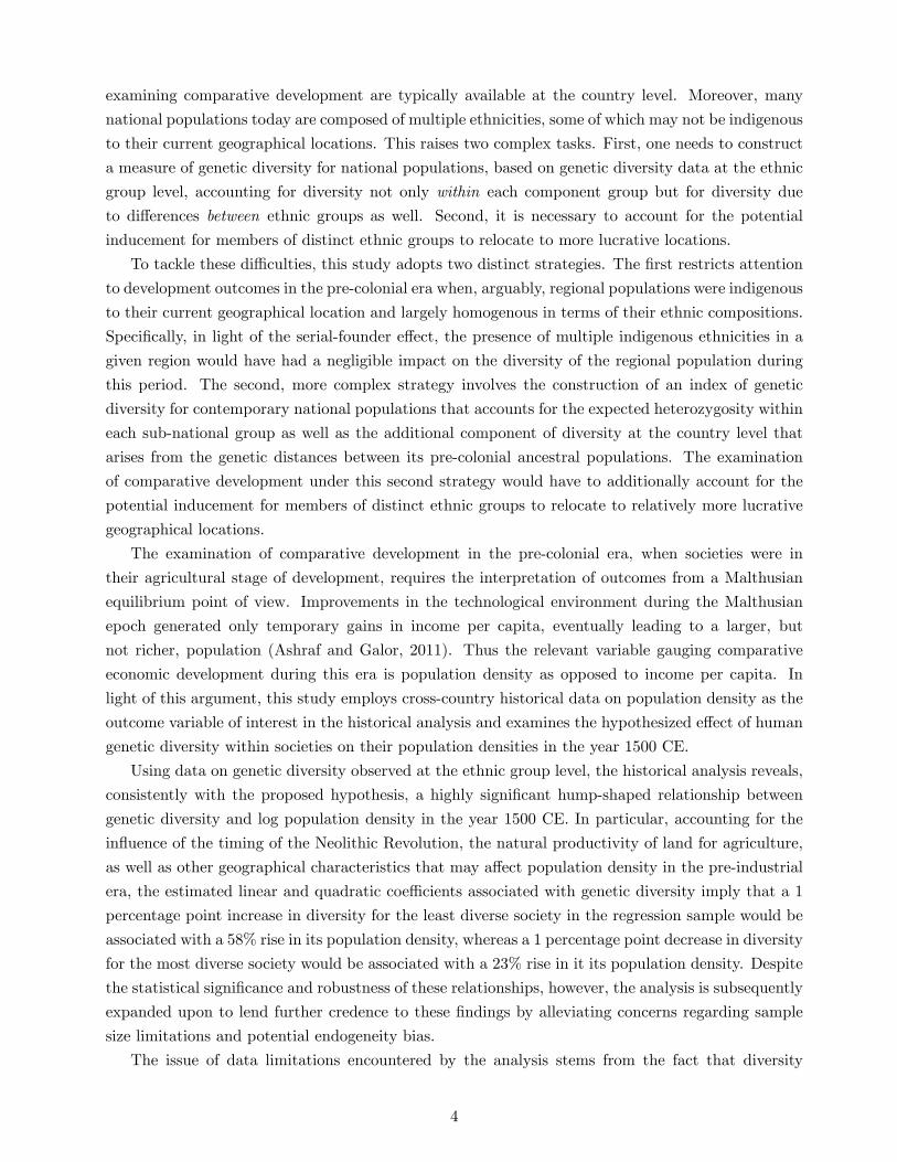
colonies. Indeed, as depicted in Figure 1, migratory distance from East Africa has an adverse e¤ect
on genetic diversity in the 53 ethnic groups across the globe that constitute the Human Genome
Diversity Cell Line Panel.
Second, there exists an optimal level of diversity for economic development, re�ecting the interplay
between the con�icting e¤ects of diversity on the development process. The adverse e¤ect pertains
to the detrimental impact of diversity on the e¢ ciency of the aggregate production process of
an economy. Heterogeneity increases the likelihood of mis-coordination and distrust, reducing
cooperation and disrupting the socioeconomic order. Greater population diversity is therefore
1

Figure 1: Expected Heterozygosity and Migratory Distance in the HGDP-CEPH Sample
associated with lower total factor productivity, which inhibits the ability of society to operate
e¢ ciently with respect to its production possibility frontier. The bene�cial e¤ect of diversity, on the
other hand, concerns the positive role of diversity in the expansion of society�s production possibility
frontier. A wider spectrum of traits is more likely to be complementary to the development and
successful implementation of advanced technological paradigms.1 Greater heterogeneity therefore
fosters the ability of a society to incorporate more sophisticated and e¢ cient modes of production,
expanding the economy�s production possibility frontier and conferring the bene�ts of increased total
factor productivity.
Higher diversity in a society�s population can therefore have con�icting e¤ects on the level of
its total factor productivity. Aggregate productivity is enhanced on the one hand by an increased
capacity for technological advancement, while diminished on the other by reduced cooperation and
e¢ ciency.2 However, if the bene�cial e¤ects of population diversity dominate at lower levels of
diversity and the detrimental e¤ects dominate at higher levels (i.e., if there are diminishing marginal
returns to both diversity and homogeneity), the theory would predict an inverted-U relationship
between genetic diversity and development outcomes throughout the development process.
The hypothesized channels through which genetic diversity a¤ects aggregate productivity follow
naturally from separate well-established mechanisms in the �eld of evolutionary biology and from
experimental evidence from scienti�c studies on organisms that display a relatively high degree
of social behavior in nature (e.g., living in task-directed hierarchical societies and engaging in
1The following two mechanisms further illustrate this argument. First, in an economy where the labor forceis characterized by genetic heterogeneity in a wide array of traits, to the extent that some of these traits leadto specialization in task-oriented activities, higher diversity will increase productivity for society as a whole, givencomplementarities across di¤erent tasks. Second, in an environment in which only individuals with su¢ ciently highlevels of cognitive abilities can contribute to technological innovation, greater variance in the distribution of these traitsacross the population will lead to higher productivity.
2This hypothesis is consistent with evidence on the costs and bene�ts associated with intra-population heterogeneity,primarily in the context of ethnic diversity, as reviewed by Alesina and La Ferrara (2005).
2

cooperative rearing of o¤spring).3 The bene�ts of genetic diversity, for instance, are highlighted in
the Darwinian theory of evolution by natural selection, according to which diversity, by permitting
the forces of natural selection to operate over a wider spectrum of traits, increases the adaptability
and, hence, the survivability of a population to changing environmental conditions.4 On the other
hand, to the extent that genetic diversity is associated with a lower average degree of relatedness
amongst individuals in a population, kin selection theory, which emphasizes that cooperation amongst
genetically-related individuals can indeed be collectively bene�cial as it ultimately facilitates the
propagation of shared genes to the next generation, is suggestive of the hypothesized mechanism
through which diversity confers costs on aggregate productivity.
In estimating the impact on economic development of migratory distance from East Africa via its
e¤ect on genetic diversity, this research overcomes issues that are presented by the existing data on
genetic diversity across the globe (i.e., measurement error and data limitations) as well as concerns
about potential endogeneity. Population geneticists typically measure the extent of diversity in
genetic material across individuals within a given population (such as an ethnic group) using an index
called expected heterozygosity. Like most other measures of diversity, this index may be interpreted
simply as the probability that two individuals, selected at random from the relevant population, are
genetically di¤erent from one another with respect to a given spectrum of traits. Speci�cally, the
expected heterozygosity measure for a given population is constructed by geneticists using sample
data on allelic frequencies, i.e., the frequency with which a �gene variant�or allele (e.g., the brown
vs. blue variant for the eye color gene) occurs in the population sample. Given allelic frequencies for
a particular gene or DNA locus, it is possible to compute a gene-speci�c heterozygosity statistic (i.e.,
the probability that two randomly selected individuals di¤er with respect to the gene in question),
which when averaged over multiple genes or DNA loci yields the overall expected heterozygosity for
the relevant population.
The most reliable and consistent data for genetic diversity among indigenous populations across
the globe consists of 53 ethnic groups from the Human Genome Diversity Cell Line Panel. According
to anthropologists, these groups are not only historically native to their current geographical location
but have also been isolated from genetic �ows from other ethnic groups. Empirical evidence provided
by population geneticists (e.g., Ramachandran et al., 2005) for these 53 ethnic groups suggest
that, indeed, migratory distance from East Africa has an adverse linear e¤ect on genetic diversity
as depicted in Figure 1. Migratory distance from East Africa for each of the 53 ethnic groups
was computed using the great circle (or geodesic) distances from Addis Ababa (Ethiopia) to the
contemporary geographic coordinates of these ethnic groups, subject to �ve obligatory intermediate
waypoints (i.e., Cairo (Egypt), Istanbul (Turkey), Phnom Penh (Cambodia), Anadyr (Russia) and
Prince Rupert (Canada)), that capture paleontological and genetic evidence on prehistorical human
migration patterns.
Nonetheless, while the existing data on genetic diversity pertain only to ethnic groups, data for
3Appendix H provides a detailed discussion of the evidence from evolutionary biology on the costs and bene�ts ofgenetic diversity.
4Moreover, according to a related hypothesis, genetically diverse honeybee colonies may operate more e¢ cientlyand productively, as a result of performing specialized tasks better as a collective, and thereby gain a �tness advantageover colonies with uniform gene pools (Robinson and Page, 1989).
3
examining comparative development are typically available at the country level. Moreover, many
national populations today are composed of multiple ethnicities, some of which may not be indigenous
to their current geographical locations. This raises two complex tasks. First, one needs to construct
a measure of genetic diversity for national populations, based on genetic diversity data at the ethnic
group level, accounting for diversity not only within each component group but for diversity due
to di¤erences between ethnic groups as well. Second, it is necessary to account for the potential
inducement for members of distinct ethnic groups to relocate to more lucrative locations.
To tackle these di¢ culties, this study adopts two distinct strategies. The �rst restricts attention
to development outcomes in the pre-colonial era when, arguably, regional populations were indigenous
to their current geographical location and largely homogenous in terms of their ethnic compositions.
Speci�cally, in light of the serial-founder e¤ect, the presence of multiple indigenous ethnicities in a
given region would have had a negligible impact on the diversity of the regional population during
this period. The second, more complex strategy involves the construction of an index of genetic
diversity for contemporary national populations that accounts for the expected heterozygosity within
each sub-national group as well as the additional component of diversity at the country level that
arises from the genetic distances between its pre-colonial ancestral populations. The examination
of comparative development under this second strategy would have to additionally account for the
potential inducement for members of distinct ethnic groups to relocate to relatively more lucrative
geographical locations.
The examination of comparative development in the pre-colonial era, when societies were in
their agricultural stage of development, requires the interpretation of outcomes from a Malthusian
equilibrium point of view. Improvements in the technological environment during the Malthusian
epoch generated only temporary gains in income per capita, eventually leading to a larger, but
not richer, population (Ashraf and Galor, 2011). Thus the relevant variable gauging comparative
economic development during this era is population density as opposed to income per capita. In
light of this argument, this study employs cross-country historical data on population density as the
outcome variable of interest in the historical analysis and examines the hypothesized e¤ect of human
genetic diversity within societies on their population densities in the year 1500 CE.
Using data on genetic diversity observed at the ethnic group level, the historical analysis reveals,
consistently with the proposed hypothesis, a highly signi�cant hump-shaped relationship between
genetic diversity and log population density in the year 1500 CE. In particular, accounting for the
in�uence of the timing of the Neolithic Revolution, the natural productivity of land for agriculture,
as well as other geographical characteristics that may a¤ect population density in the pre-industrial
era, the estimated linear and quadratic coe¢ cients associated with genetic diversity imply that a 1
percentage point increase in diversity for the least diverse society in the regression sample would be
associated with a 58% rise in its population density, whereas a 1 percentage point decrease in diversity
for the most diverse society would be associated with a 23% rise in it its population density. Despite
the statistical signi�cance and robustness of these relationships, however, the analysis is subsequently
expanded upon to lend further credence to these �ndings by alleviating concerns regarding sample
size limitations and potential endogeneity bias.
The issue of data limitations encountered by the analysis stems from the fact that diversity
4

data at the ethnic group level currently spans only a modest subset of the sample of countries
for which historical population estimates are available. The potential endogeneity issue, on the
other hand, arises from the possibility that genetic diversity within populations could partly re�ect
historical processes such as interregional migrations that were, in turn, determined by historical
patterns of comparative development. Furthermore, the direction of the potential endogeneity
bias is a priori ambiguous. For example, while historically better developed regions may have
been attractive destinations to potential migrants, serving to increase genetic diversity in relatively
wealthier societies, the more advanced technologies in these societies may also have conferred the
necessary military prowess to prevent or minimize foreign invasions, thereby reducing the likelihood
of greater genetic diversity in their populations.5
In surmounting the aforementioned data limitations and potential endogeneity issues, this re-
search appeals to the �out of Africa� theory regarding the origins of Homo sapiens. According to
this well-established hypothesis, the human species, having evolved to its modern form in East Africa
some 150,000 years ago, thereafter embarked on populating the entire globe in a stepwise migration
process beginning about 70,000�90,000 BP.6 Using archeological data combined with mitochondrial
and Y-chromosomal DNA analysis to identify the most recent common ancestors of contemporary
human populations, geneticists are able to not only o¤er evidence supporting the origin of humans
in East Africa but also trace the prehistorical migration routes of the subsequent human expansion
into the rest of the world. In addition, population geneticists studying human genetic diversity have
argued that the contemporary distribution of diversity across populations should re�ect a serial-
founder e¤ect originating in East Africa. Accordingly, since the populating of the world occurred in
a series of stages where subgroups left initial colonies to create new colonies further away, carrying
with them only a portion of the overall genetic diversity of their parental colonies, contemporary
genetic diversity in human populations should be expected to decrease with increasing distance along
prehistorical migratory paths from East Africa.7 Indeed, several studies in population genetics (e.g.,
Prugnolle et al., 2005; Ramachandran et al., 2005; Wang et al., 2007) have found strong empirical
evidence in support of this prediction.
5The history of world civilization is abound with examples of both phenomena. The �Barbarian Invasions�of theWestern Roman Empire in the Early Middle Ages is a classic example of historical population di¤usion occurring alonga prosperity gradient, whereas the The Great Wall of China, built and expanded over centuries to minimize invasionsby nomadic tribes, serves (literally) as a landmark instance of the latter phenomenon.
6An alternative to this �recent African origin� (RAO) model is the �multiregional evolution accompanied by gene�ow� hypothesis, according to which early modern hominids evolved independently in di¤erent regions of the worldand thereafter exchanged genetic material with each other through migrations, ultimately giving rise to a relativelyuniform dispersion of modern Homo sapiens throughout the globe. However, in light of surmounting genetic andpaleontological evidence against it, the multiregional hypothesis has by now almost completely lost ground to the RAOmodel of modern human origins (Stringer and Andrews, 1988).
7 In addition, population geneticists argue that the reduced genetic diversity associated with the founder e¤ect isdue not only to the subset sampling of alleles from parental colonies but also to a stronger force of �genetic drift�that operates on the new colonies over time. Genetic drift arises from the fundamental tendency of the frequency ofany allele in an inbreeding population to vary randomly across generations as a result of random statistical samplingerrors alone (i.e., the random production of a few more or less progeny carrying the relevant allele). Thus, given theinherent �memoryless� (Markovian) property of allelic frequencies across generations, the process ultimately leads, inthe absence of mutation and natural selection, to either a 0% or a 100% representation of the allele in the population(Gri¢ ths et al., 2000). Moreover, since random sampling errors are more prevalent in circumstances where the lawof large numbers is less applicable, genetic drift is more pronounced in smaller populations, thereby allowing thisphenomenon to play a signi�cant role in the founder e¤ect.
5
The present study exploits the explanatory power of migratory distance from East Africa for
genetic diversity within ethnic groups in order to overcome the data limitations and potential
endogeneity issues encountered by the initial analysis discussed above. In particular, the strong
ability of prehistorical migratory distance from East Africa in explaining observed genetic diversity
permits the analysis to generate predicted values of genetic diversity using migratory distance for
countries for which diversity data are currently unavailable. This enables a subsequent analysis to
estimate the e¤ects of genetic diversity, as predicted by migratory distance from East Africa, in a
much larger sample of countries. Moreover, given the obvious exogeneity of migratory distance from
East Africa with respect to development outcomes in the Common Era, the use of migratory distance
to project genetic diversity alleviates concerns regarding the potential endogeneity between observed
genetic diversity and economic development.
The main results from the historical analysis, employing predicted genetic diversity in the ex-
tended sample of countries, indicate that, controlling for the in�uence of land productivity, the timing
of the Neolithic Revolution, and continental �xed e¤ects, a 1 percentage point increase in diversity
for the most homogenous society in the sample would raise its population density in 1500 CE by
36%, whereas a 1 percentage point decrease in diversity for the most diverse society would raise its
population density by 29%. Further, a 1 percentage point change in diversity in either direction at
the predicted optimum of 0.683 would lower population density by 1.5%.8
Moving to the contemporary period, the analysis, as discussed earlier, constructs an index of
genetic diversity at the country level that not only incorporates the expected heterozygosities of
the pre-Columbian ancestral populations of contemporary sub-national groups, as predicted by the
migratory distances of the ancestral populations from East Africa, but also incorporates the pairwise
genetic distances between these ancestral populations, as predicted by their pairwise migratory
distances. Indeed, the serial-founder e¤ect studied by population geneticists not only predicts that
expected heterozygosity declines with increasing distance along migratory paths from East Africa, but
also that the genetic distance between any two populations will be larger the greater the migratory
distance between them.
The baseline results from the contemporary analysis indicate that the genetic diversity of con-
temporary national populations has an economically and statistically signi�cant hump-shaped e¤ect
on income per capita. This hump-shaped impact is robust to controls for continental �xed e¤ects,
ethnic fractionalization, various measures of institutional quality (i.e., social infrastructure, an index
gauging the extent of democracy, and constraints on the power of chief executives), legal origins,
major religion shares, the share of the population of European descent, years of schooling, disease
environments, and other geographical factors that have received attention in the empirical literature
on cross-country comparative development.
The direct e¤ect of genetic diversity on contemporary income per capita, once institutional,
8Consistent with the predictions of the proposed hypothesis, the robustness analysis in Appendix A demonstratesthat the non-monotonic e¤ect of genetic diversity on development outcomes is prevalent in earlier historical periodsas well. Moreover, genetic diversity explains between 5% and 38% of the cross-country variation in log populationdensity, depending on the historical period examined and the control variables included in the regression speci�cation.Indeed, the impact of genetic diversity is robust to various regression speci�cations such as the inclusion of controlsfor the spatial in�uence of regional technological frontiers via trade and the di¤usion of technologies, and controls formicrogeographic factors gauging terrain quality and proximity to waterways.
6

cultural, and geographical factors are accounted for, indicates that: (i) increasing the diversity of
the most homogenous country in the sample (Bolivia) by 1 percentage point would raise its income
per capita in the year 2000 CE by 39%, (ii) decreasing the diversity of the most diverse country
in the sample (Ethiopia) by 1 percentage point would raise its income per capita by 21%, (iii) a
1 percentage point change in genetic diversity (in either direction) at the optimum level of 0.721
(that most closely resembles the diversity level of the U.S.) would lower income per capita by 1.9%,
(iv) increasing Bolivia�s diversity to the optimum level prevalent in the U.S. would increase Bolivia�s
per capita income by a factor of 4.7, closing the income gap between the U.S. and Bolivia from a
ratio of 12:1 to 2.5:1, and (v) decreasing Ethiopia�s diversity to the optimum level of the U.S. would
increase Ethiopia�s per capita income by a factor of 1.7 and, thus, close the income gap between
the U.S. and Ethiopia from a ratio of 47:1 to 27:1. Moreover, the partial R-squared associated with
diversity suggests that residual genetic diversity explains about 15% of the cross-country variation in
residual log income per capita in 2000 CE, conditional on the institutional, cultural, and geographical
covariates in the baseline regression model.
Reassuringly, the highly signi�cant and stable hump-shaped e¤ect of genetic diversity on income
per capita in the year 2000 CE is not an artifact of post-colonial migrations towards prosperous
countries and the concomitant increase in ethnic diversity in these economies. The hump-shaped
e¤ect of genetic diversity remains highly signi�cant and the optimal diversity estimate remains
virtually intact if the regression sample is restricted to (a) non-OECD economies (i.e., economies
that were less attractive to migrants), (b) non Neo-European countries (i.e., excluding the U.S.,
Canada, New Zealand and Australia), (c) non-Latin American countries, (d) non Sub-Saharan
African countries, and perhaps most importantly (e) to countries whose indigenous population is
larger than 97% of the entire population (i.e., under conditions that virtually eliminate the role of
migration in the creation of diversity). Moreover, consistently with the overall hump-shaped e¤ect
of diversity on the contemporary standard of living, the analysis indicates that genetic diversity
is negatively associated with the extent of cooperative behavior, as measured by the prevalence of
interpersonal trust, and positively associated with innovative activity, as measured by the intensity
of scienti�c knowledge creation.
The remainder of the paper is organized as follows: Section 1 brie�y reviews some related
literature. Section 2 presents a basic model that predicts a hump-shaped e¤ect of diversity on
economic development. Section 3 covers the historical analysis, discussing the empirical strategy as
well as the relevant data and data sources before presenting the empirical �ndings. Section 4 does
the same for the contemporary analysis, and, �nally, Section 5 concludes.
1 Related Literature
The existing literature on comparative development has emphasized a variety of factors underlying
some of the vast di¤erences in living standards across the globe. The in�uence of geography, for
instance, has been stressed from a historical perspective by Jones (1981), Diamond (1997), and
Pomeranz (2000), and is highlighted empirically by Gallup et al. (1999) and Olsson and Hibbs
(2005), amongst others. Institutions, on the other hand, are given historical precedence by North and
7

Thomas (1973), Mokyr (1990), and Greif (1993), and are emphasized empirically by Hall and Jones
(1999), La Porta et al. (1999), Rodrik et al. (2004), and Acemoglu et al. (2005). In related strands
of the literature on institutions, Engerman and Sokolo¤ (2000) and Acemoglu et al. (2005) have
stressed the role of colonialism, while the e¤ects of ethno-linguistic fractionalization are examined
by Easterly and Levine (1997), Alesina et al. (2003), and others. Meanwhile, the historical impact
of sociocultural factors has been highlighted by Weber (1905) and Landes (1998), with empirical
support coming from Barro and McCleary (2003), Tabellini (2008), as well as Guiso et al. (2009).
Finally, the importance of human capital formation has been underlined in uni�ed growth theory
(e.g., Galor, 2011), and has been demonstrated empirically by Glaeser et al. (2004).9
This research is the �rst to argue that the variation in prehistorical migratory distance from the
cradle of humankind to various settlements across the globe has had a persistent e¤ect on the process
of development and on the contemporary variation in income per capita across the globe. The paper
is also unique in its attempt to establish the role of genetic (rather than ethnic) diversity within
a society as a signi�cant determinant of its development path and, thus, its comparative economic
performance across space and time.
The employment of data and empirical results from the �eld of population genetics places this
research in the neighborhood of a recent insightful paper by Spolaore and Wacziarg (2009) who
have appealed to data on genetic distance between human populations to proxy for the e¤ect of
sociocultural di¤erences between societies on the di¤usion of economic development.10 Speci�cally,
the authors argue that genetic distance between populations, which captures their divergence in
biological and cultural characteristics over time, has been a barrier to the horizontal di¤usion of
technological innovations across populations. They show that Fst genetic distance, a measure that
re�ects the time elapsed since two populations shared a common ancestor, confers a statistically
signi�cant positive e¤ect on both historical and contemporary pairwise income di¤erences. In
contrast, the genetic diversity metric within populations exploited by this paper facilitates the
analysis of the e¤ect of the variation in traits across individuals within a society on its development
process.
Unlike Spolaore and Wacziarg (2009) where genetic distance between populations diminishes the
rate of technological di¤usion and reduces productivity, the hypothesis advanced and tested by the
current analysis suggests that genetic diversity within a population confers both social costs, in the
form of lower social capital arising from di¤erences amongst individual members, and social bene�ts
in the form of diversity-driven knowledge accumulation. Hence, the overall e¤ect of genetic diversity
on developmental outcomes would be hump-shaped, rather than monotonically negative. The results
of the empirical analysis conducted in this study suggest that the previously unexamined bene�cial
e¤ect of genetic di¤erences is indeed a signi�cant factor in the overall in�uence of the genetic channel
on comparative development.
The examination of the e¤ects of genetic diversity along with the in�uence of the timing of9See also Dalgaard and Strulik (2010).10See also Desmet et al. (2011) who demonstrate a strong correlation between genetic and cultural distances among
European populations to argue that genetic distance can be employed as an appropriate proxy to study the e¤ect ofcultural distance on the formation of new political borders in Europe. In addition, an earlier version of the study byGuiso et al. (2009) employs data on genetic distance between European populations as an instrument for measures oftrust to estimate its e¤ect on the volume of bilateral trade and foreign direct investment.
8

agricultural transitions also places this paper in an emerging strand of the literature that has
focused on empirically testing Diamond�s (1997) assertion regarding the long-standing impact of
the Neolithic Revolution.11 Diamond (1997) has stressed the role of biogeographical factors in
determining the timing of the Neolithic Revolution, which conferred a developmental head-start
to societies that experienced an earlier transition from primitive hunting and gathering techniques
to the more technologically advanced agricultural mode of production. According to this hypothesis,
the luck of being dealt a favorable hand thousands of years ago with respect to biogeographic
endowments, particularly exogenous factors contributing to the emergence of agriculture and facili-
tating the subsequent di¤usion of agricultural techniques, is the single most important driving force
behind the divergent development paths of societies throughout history that ultimately led to the
contemporary global di¤erences in standards of living. Speci�cally, an earlier transition to agriculture
due to favorable environmental conditions gave some societies an early advantage by conferring the
bene�ts of a production technology that generated resource surpluses and enabled the rise of a
non-food-producing class whose members were crucial for the development of written language and
science, and for the formation of cities, technology-based military powers and nation states. The
early technological dominance of these societies subsequently persisted throughout history, being
further sustained by the subjugation of less-developed societies through exploitative geopolitical and
historical processes such as colonization.
While the long-standing in�uence of the Neolithic Revolution on comparative development re-
mains a compelling argument, this research demonstrates that, contrary to Diamond�s (1997) uni-
causal hypothesis, the composition of human populations with respect to their genetic diversity has
been an signi�cant and persistent factor that a¤ected the course of economic development from the
dawn of human civilization to the present. In estimating the economic impact of human genetic
diversity while controlling for the channel emphasized by Diamond (1997), the current research
additionally establishes the historical signi�cance of the timing of agricultural transitions for pre-
colonial population density, which, as already argued, is the relevant variable capturing comparative
economic development during the Malthusian epoch of stagnation in income per capita.12
2 Diversity and Productivity: A Basic Model
Consider an economy where the level of productivity is a¤ected by the degree of genetic diversity in
society. Speci�cally, genetic diversity generates con�icting e¤ects on productivity. A wider spectrum
of traits is complementary to the adoption or implementation of new technologies. It enhances
11See, for example, Olsson and Hibbs (2005) and Putterman (2008).12Note that, although the genetic diversity channel raised in this study is conceptually independent of the timing
of the agricultural transition, an additional genetic channel that interacts with the time elapsed since the NeolithicRevolution has been examined by Galor and Moav (2002, 2007). These studies argue that the Neolithic transitiontriggered an evolutionary process resulting in the natural selection of certain genetic traits (such as preference forhigher quality children and greater longevity) that are complementary to economic development, thereby implying aceteris paribus positive relationship between the timing of the agricultural transition and the representation of suchtraits in the population. Indeed, the empirical evidence recently uncovered by Galor and Moav (2007) is consistent withthis theoretical prediction. Thus, while the signi�cant reduced-form e¤ect of the Neolithic Revolution observed in thisstudy may be associated with the Diamond hypothesis, it could also be partly capturing the in�uence of this additionalgenetic channel. See also Lagerlöf (2007) and Galor and Michalopoulos (2011) for complementary evolutionary theoriesregarding the dynamics of human body mass and entrepreneurial spirit in the process of economic development.
9

knowledge creation and fosters technological progress, thereby expanding the economy�s production
possibility frontier. However, a wider spectrum of traits also reduces the likelihood of cooperative or
trustful behavior, generating ine¢ ciencies in the operation of the economy relative to its production
possibility frontier.
Suppose that the degree of genetic diversity, ! 2 [0; 1], has a positive but diminishing e¤ect
on the level of technology that is available for production. Speci�cally, the level of technology, A,
and thus the economy�s production possibility frontier, is determined by a vector of institutional,
geographical, and human capital factors, z, as well as by the degree of diversity, !.13
A = A(z; !), (1)
where A(z; !) > 0, A!(z; !) > 0, and A!!(z; !) < 0 for all ! 2 [0; 1], and lim!�!0A!(z; !) = 1and lim!�!1A!(z; !) = 0.
Suppose further that the position of the economy relative to its production possibly frontier is
adversely a¤ected by the degree of genetic diversity. In particular, a fraction, �!, of the economy�s
potential productivity, A(z; !), is lost due to lack of cooperation and resultant ine¢ ciencies in the
production process.
Output per worker is therefore determined by the level of employment of factors of production,
x, the level of productivity, A(z; !), and the degree of ine¢ ciency in production, � 2 (0; 1).
y = (1� �!)A(z; !)f(x) � y(!), (2)
where x is a vector of factor inputs per worker, and �! is the extent of erosion in productivity due
to ine¢ ciencies in the production process.14 Hence, as follows from (2), y(!) is a strictly concave
hump-shaped function of !. Speci�cally,
y0(!) = [(1� �!)A!(z; !)� �A(z; !)]f(x);
y00(!) = [(1� �!)A!!(z; !)� 2�A!(z; !)]f(x) < 0;
lim!�!0 y0(!) > 0; and lim!�!1 y0(!) < 0.
(3)
Thus, there exists an intermediate level of diversity, !� 2 (0; 1), that maximizes the level of
13Several mechanisms could generate this reduced form relationship. Suppose that the labor force is characterizedby heterogeneity in equally productive traits, each of which permit individuals to perform complementary specializedtasks. The quantity of trait i in the population is xi and it is distributed uniformly over the interval [0; !]. The levelof productivity is therefore,
A(z; !) = z
Z !
0
x�i di; � 2 (0; 1).
Hence, an increase in the spectrum of traits, !, (holding the aggregate supply of productive traits constant) will increaseproductivity at a diminishing rate. Alternatively, if there exists a hierarchy of traits and only traits above the cut-o¤� 2 (0; !) contribute to productivity, then an increase in the spectrum of traits, !, could increase productivity at adiminishing rate.14 If degree of ine¢ ciency is �(!), the results of the model would remain intact as long as the contribution of
homogeneity for e¢ ciency is diminishing (i.e., as long as �(!) is non-decreasing and weakly convex in !).
10

output per worker. In particular, !� satis�es
(1� �!�)A!(z; !�) = �A(z; !�). (4)
3 The Historical Analysis
3.1 Data and Empirical Strategy
This section discusses the data and empirical strategy employed to examine the impact of genetic
diversity on comparative development in the pre-colonial era.
3.1.1 Dependent Variable: Historical Population Density
As argued previously, the relevant variable re�ecting comparative development across countries in
the pre-colonial Malthusian era is population density. The empirical examination of the proposed
genetic hypothesis therefore aims to employ cross-country variation in observed genetic diversity
and in that predicted by migratory distance from East Africa to explain cross-country variation in
historical population density.15 Data on historical population density are obtained from McEvedy
and Jones (1978) who provide �gures at the country level, i.e., for regions de�ned by contemporary
national borders, over the period 400 BCE�1975 CE.16 However, given the greater unreliability (and
less availability in terms of observations) of population data for earlier historical periods, the baseline
regression speci�cation adopts population density in 1500 CE as the preferred outcome variable to
examine. The analysis in Appendix A additionally examines population density in 1000 CE and 1
CE to demonstrate the robustness of the genetic channel for earlier time periods.
3.1.2 Independent Variable: Genetic Diversity
The most reliable and consistent data for genetic diversity among indigenous populations across the
globe consists of 53 ethnic groups from the Human Genome Diversity Cell Line Panel, compiled
by the Human Genome Diversity Project-Centre d�Etudes du Polymorphisme Humain (HGDP-
CEPH).17 According to anthropologists, these 53 ethnic groups are not only historically native
to their current geographical location but have also been isolated from genetic �ows from other
ethnic groups. Population geneticists typically measure the extent of diversity in genetic material
across individuals within a given population (such as an ethnic group) using an index called expected
heterozygosity. Like most other measures of diversity, this index may be interpreted simply as the
probability that two individuals, selected at random from the relevant population, are genetically
di¤erent from one another. Speci�cally, the expected heterozygosity measure for a given population
15Admittedly, historical data on population density is a icted by measurement error. However, while measurementerror in explanatory variables leads to attenuation bias in OLS estimators, mismeasurement of the dependent variablein an OLS regression, as a result of yielding larger standard errors for coe¢ cient estimates, leads to rejecting the nullwhen it is in fact true. As such, if OLS coe¢ cients are precisely estimated, then con�dence that the true coe¢ cientsare indeed di¤erent from zero rises even in the presence of measurement error in the dependent variable.16The reader is referred to Appendix F for additional details.17For a more detailed description of the HGDP-CEPH Human Genome Diversity Cell Line Panel data set, the
interested reader is referred to Cann et al. (2002). A broad overview of the Human Genome Diversity Project is givenby Cavalli-Sforza (2005). The 53 ethnic groups are listed in Appendix E.
11

is constructed by geneticists using sample data on allelic frequencies, i.e., the frequency with which a
�gene variant�or allele occurs in the population sample. Given allelic frequencies for a particular gene
or DNA locus, it is possible to compute a gene-speci�c heterozygosity statistic (i.e., the probability
that two randomly selected individuals di¤er with respect to a given gene), which when averaged over
multiple genes or DNA loci yields the overall expected heterozygosity for the relevant population.18
Consider a single gene or locus l with k observed variants or alleles in the population and let pidenote the frequency of the i-th allele. Then, the expected heterozygosity of the population with
respect to locus l, H lexp, is:
H lexp = 1�
kXi=1
p2i . (5)
Given allelic frequencies for each of m di¤erent genes or loci, the average across these loci then
yields an aggregate expected heterozygosity measure of overall genetic diversity, Hexp, as:
Hexp = 1�1
m
mXl=1
klXi=1
p2i , (6)
where kl is the number of observed variants in locus l.
Empirical evidence uncovered by Ramachandran et al. (2005) for the 53 ethnic groups from the
Human Genome Diversity Cell Line Panel suggests that migratory distance from East Africa has
an adverse linear e¤ect on genetic diversity. They interpret this �nding as providing support for a
serial-founder e¤ect originating in East Africa, re�ecting a process where the populating of the world
occurred in a series of discrete steps involving subgroups leaving initial settlements to establish new
settlements further away and carrying with them only a subset of the overall genetic diversity of
their parental colonies.
In estimating the migratory distance from East Africa for each of the 53 ethnic groups in their
data set, Ramachandran et al. (2005) calculate great circle (or geodesic) distances using Addis
Ababa (Ethiopia) as the point of common origin and the contemporary geographic coordinates of the
18 It should be noted that sources other than HGDP-CEPH exist for expected heterozygosity data. Speci�cally, theonline Allele Frequency Database (ALFRED) represents one of the largest repositories of such data, pooled from acrossdi¤erent data sets used by numerous studies in human population genetics. However, the data from ALFRED, whilecorresponding to a much larger sample of populations (ethnic groups) than the HGDP-CEPH sample, are problematicfor a number of reasons. First, the expected heterozygosity data in ALFRED are not comparable across populationsfrom the individual data sets in the collection because they are based on di¤erent DNA sampling methodologies (asdictated by the scienti�c goals of the di¤erent studies). Second, the vast majority of the individual data sets in ALFREDdo not provide global coverage in terms of the di¤erent populations that are sampled and, even when they do, thesample size is considerably less than that of the HGDP-CEPH panel. Third, in comparison to the 783 loci employedby Ramachandran et al. (2005) to compute the expected heterozygosities for the 53 HGDP-CEPH populations, thosereported for the non-HGDP populations in ALFRED are on average based on allelic frequencies for less than 20 DNAloci, which introduces a signi�cant amount of potentially systematic noise in the heterozygosity estimates for theseother populations. Fourth, unlike the microsatellite loci used by Ramachandran et al. (2005) for the HGDP-CEPHpopulations, the expected heterozygosities reported for many non-HGDP populations in ALFRED capture allelicvariations across individuals in loci that reside in protein-coding regions of the human genome, thus re�ecting diversityin phenotypic expressions that may have been subject to the environmental forces of natural selection. Finally, incontrast to the HGDP-CEPH populations, many of the non-HGDP populations in ALFRED represent ethnic groupsthat have experienced signi�cant genetic admixture in their recent histories, particularly during the post-Columbianera, and this introduces an endogeneity problem for the current analysis since genetic admixtures are, in part, theresult of migrations occurring along spatial economic prosperity gradients.
12

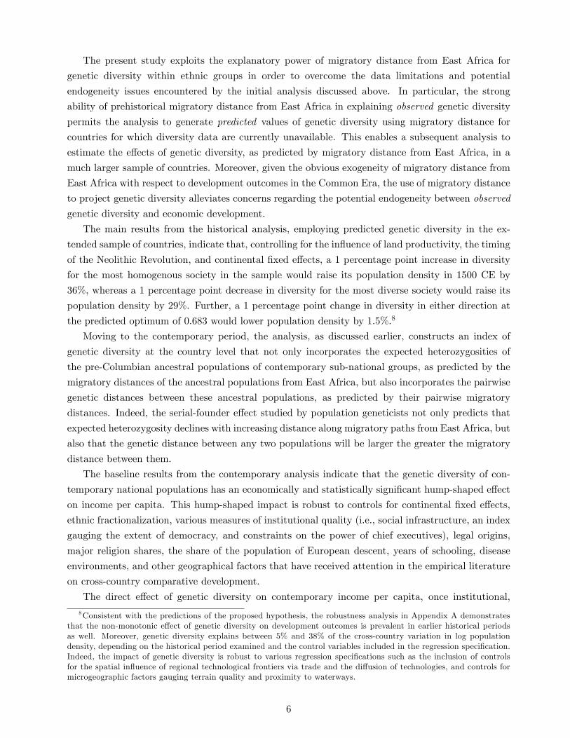
Figure 2: The 53 HGDP-CEPH Ethnic Groups and Migratory Paths from East Africa
sampled groups as the destinations. Moreover, these distance estimates incorporate �ve obligatory
intermediate waypoints, used to more accurately capture paleontological and genetic evidence on
prehistorical human migration patterns that are consistent with the widely-held hypothesis that,
in the course of their exodus from Africa, humans did not cross large bodies of water. The inter-
mediate waypoints, depicted on the world map in Figure 2 along with the spatial distribution of
the ethnic groups from the HGDP-CEPH sample, are: Cairo (Egypt), Istanbul (Turkey), Phnom
Penh (Cambodia), Anadyr (Russia) and Prince Rupert (Canada). For instance, as illustrated in
Figure 2, the migration path from Addis Ababa to the Papuan ethnic group in modern-day New
Guinea makes use of Cairo and Phnom Penh whereas that to the Karitiana population in Brazil
incorporates Cairo, Anadyr and Prince Rupert as intermediate waypoints.19 The migratory distance
between endpoints (i.e., Addis Ababa and the location of a group) is therefore the sum of the great
circle distances between these endpoints and the waypoint(s) in the path connecting them, and the
distance(s) between waypoints if two or more such points are required.
The empirical analysis of Ramachandran et al. (2005) establishes migratory distance from East
Africa as a strong negative predictor of genetic diversity at the ethnic group level. Based on the
R-squared of their regression, migratory distance alone explains almost 86% of the cross-group
variation in within-group diversity.20 In addition, the estimated OLS coe¢ cient is highly statistically
19Based on mitochondrial DNA analysis, some recent studies (e.g., Macaulay et al., 2005) have proposed a southernexit route out of Africa whereby the initial exodus into Asia occurred not via the Levant but across the mouth ofthe Red Sea (between modern-day Djibouti and Yemen), thereafter taking a �beachcombing�path along the southerncoast of the Arabian Peninsula to India and onward into Southeast Asia. Moreover, a subsequent northern o¤shootfrom the Persian Gulf region ultimately lead to the settlement of the Near East and Europe. This scenario thereforesuggests the use of Sana�a (Yemen) and Bandar Abbas (Iran) as intermediate waypoints instead of Cairo. Adoptingthis alternative route for computing migratory distances, however, does not qualitatively alter the main results.20These results are similar to those uncovered in an independent study by Prugnolle et al. (2005) that employs a
subset of the HGDP-CEPH sample encompassing 51 ethnic groups whose expected heterozygosities are calculated fromallelic frequencies for 377 loci. Despite their somewhat smaller sample at both the ethnic group and DNA analysislevels, Prugnolle et al. (2005) �nd that migratory distance from East Africa explains 85% of the variation in geneticdiversity. On the other hand, using an expanded data set comprised of the 53 HGDP-CEPH ethnic groups and an
13

signi�cant, possessing a t-statistic = -9.770 (P-value < 10�4), and suggests that predicted expected
heterozygosity falls by 0.076 percentage points for every 10,000 km increase in migratory distance
from Addis Ababa.21 This is the relationship depicted earlier in Figure 1.
The present study exploits the explanatory power of migratory distance from East Africa for the
cross-sectional variation in ethnic group expected heterozygosity in order to advance the empirical
analysis of the e¤ect of diversity on development in two dimensions. First, given the potential
endogeneity between observed genetic diversity and economic development as discussed earlier, the
use of genetic diversity values predicted by migratory distance from East Africa alleviates concerns
regarding endogeneity bias. Speci�cally, the identifying assumption being employed here is that
distances along prehistorical human migration routes from Africa have no direct e¤ect on economic
development during the Common Era. Second, the strong capacity of migratory distance in predicting
genetic diversity implies that the empirical analysis of the genetic hypothesis proposed in this study
need not be restricted to the 53 HGDP-CEPH ethnic groups that span only 21 countries, especially
since data on the outcome variable of interest (i.e., population density in the year 1500 CE) are
available for a much larger set of countries.
To further elaborate, the current analysis tests the proposed genetic hypothesis both using
observed genetic diversity in a limited sample of 21 countries, spanned by the 53 ethnic groups
in the HGDP-CEPH data set, and using genetic diversity predicted by migratory distance from
East Africa in an extended sample of 145 countries. In the 21-country sample, genetic diversity
and migratory distance are aggregated up to the country level by averaging across the set of ethnic
groups located within a given country.22 For the extended sample, however, the distance calculation
methodology of Ramachandran et al. (2005) is adopted to �rst construct migratory distance from
East Africa for each country, using Addis Ababa as the origin and the country�s modern capital city
as the destination along with the aforementioned waypoints for restricting the migration route to
landmasses as much as possible.23 This constructed distance variable is then applied to obtain a
predicted value of genetic diversity for each country based on the coe¢ cient on migratory distance
in Ramachandran et al.�s (2005) regression across the 53 HGDP-CEPH ethnic groups. Hence, it is
this predicted genetic diversity at the country level that is employed as the explanatory variable of
additional 24 Native American populations, Wang et al. (2007) �nd that migratory distance explains a more modest74% of the variation in genetic diversity, based on allelic frequencies for 678 loci. The authors attribute their somewhatweaker results to the fact that the additional Native American ethnic groups in their augmented sample were historicallysubjected to a high degree of gene �ow from foreign populations (i.e., European colonizers), which obscured the geneticlegacy of a serial-founder e¤ect in these groups.21This e¤ect corresponds to roughly one-third of the full (worldwide) range of expected heterozygosity values observed
across the HGDP-CEPH sample of ethnic groups.22A population-weighted averaging method is infeasible in this case due to the current unavailability of population
�gures for the HGDP-CEPH ethnic groups.23Clearly, there is some amount of measurement error that is introduced by following this methodology since actual
migration paths are only approximated due to the use of �ve major intercontinental waypoints. For instance, using thisgeneral method to calculate the migratory distance to Iceland, which was settled in the 9th century CE by a Norwegianpopulation, fails to capture Oslo as an additional case-speci�c waypoint. The overall sparsity of historical evidence,however, regarding the actual source of initial settlements in many regions makes a more re�ned analysis infeasible.Nonetheless, it is credibly postulated that the absence of case-speci�c waypoints from the analysis does not introducesigni�cant mismeasurement at the global scale. The same argument applies in defense of using modern capital citiesas destination points for the migratory paths, although historical evidence suggests that, at least for many cases in the�Old World�, modern capitals were also some of the major centers of urbanization throughout the Common Era (see,e.g., Bairoch, 1988; McEvedy and Jones, 1978).
14

interest in the extended sample of countries.24
3.1.3 Control Variables: Neolithic Transition Timing and Land Productivity
Diamond�s (1997) hypothesis has identi�ed the timing of the Neolithic Revolution as a proximate
determinant of economic development, designating initial geographic and biogeographic conditions
that governed the emergence and adoption of agricultural practices in prehistorical hunter-gatherer
societies as the ultimate determinants in this channel. Some of these geographic and biogeographic
factors, highlighted in the empirical analysis of Olsson and Hibbs (2005), include the size of the
continent or landmass, the orientation of the major continental axis, type of climate, and the number
of prehistorical plant and animal species amenable for domestication.
The current analysis controls for the ultimate and proximate determinants of development in
the Diamond channel using cross-country data on the aforementioned geographic and biogeographic
variables as well as on the timing of the Neolithic Revolution.25 However, given the empirical
link between the ultimate and proximate factors in Diamond�s hypothesis, the baseline speci�cation
focuses on the timing of the Neolithic transition to agriculture as the relevant control variable for
this channel. The results from an extended speci�cation that incorporates initial geographic and
biogeographic factors as controls are presented in Appendix A to demonstrate robustness.
The focus of the historical analysis on economic development in the pre-colonial Malthusian
era also necessitates controls for the natural productivity of land for agriculture. Given that in a
Malthusian environment resource surpluses are primarily channeled into population growth with per
capita incomes largely remaining at or near subsistence, regions characterized by natural factors
generating higher agricultural crop yields should, ceteris paribus, also exhibit higher population
densities (Ashraf and Galor, 2011).26 If diversity in a society in�uences its development through total
factor productivity (comprised of both social capital and technological know-how), then controlling
for the natural productivity of land would constitute a more accurate test of the e¤ect of diversity
24As argued by Pagan (1984) and Murphy and Topel (1985), the OLS estimator for this two-step estimation methodyields consistent estimates of the coe¢ cients in the second stage regression, but inconsistent estimates of their standarderrors as it fails to account for the presence of a generated regressor. This inadvertently causes naive statistical inferencesto be biased in favor of rejecting the null hypothesis. To surmount this issue, the current study employs a two-stepbootstrapping algorithm to compute the standard errors in all regressions that use the extended sample containingpredicted genetic diversity at the country level. The bootstrap estimates of the standard errors are constructed in thefollowing manner. A random sample with replacement is drawn from the HGDP-CEPH sample of 53 ethnic groups. The�rst stage regression is estimated on this random sample and the corresponding OLS coe¢ cient on migratory distanceis used to compute predicted genetic diversity in the extended sample of countries. The second stage regression isthen estimated on a random sample with replacement drawn from the extended cross-country sample and the OLScoe¢ cients are stored. This process of two-step bootstrap sampling and least squares estimation is repeated 1,000times. The standard deviations in the sample of 1,000 observations of coe¢ cient estimates from the second stageregression are thus the bootstrap standard errors of the point estimates of these coe¢ cients.25The data source for the aforementioned geographic and biogeographic controls is Olsson and Hibbs (2005) whereas
that for the timing of the Neolithic Revolution is Putterman (2008). See Appendix F for the de�nitions and sources ofall primary and control variables employed by the analysis.26 It is important to note, in addition, that the type of land productivity being considered here is largely independent of
initial geographic and biogeographic endowments in the Diamond channel and, thus, somewhat orthogonal to the timingof agricultural transitions as well. This holds due to the independence of natural factors conducive to domesticatedspecies from those that were bene�cial for the wild ancestors of eventual domesticates. As argued by Diamond (2002),while agriculture originated in regions of the world to which the most valuable domesticable wild plant and animalspecies were native, other regions proved more fertile and climatically favorable once the di¤usion of agriculturalpractices brought the domesticated varieties to them.
15

on the Malthusian development outcome �i.e., population density.
In controlling for the agricultural productivity of land, this study employs measurements of three
geographic variables at the country level including (i) the percentage of arable land, (ii) absolute
latitude, and (iii) an index gauging the overall suitability of land for agriculture based on ecological
indicators of climate suitability for cultivation, such as growing degree days and the ratio of actual
to potential evapotranspiration, as well as ecological indicators of soil suitability for cultivation, such
as soil carbon density and soil pH.27
3.1.4 The Baseline Regression Speci�cations
In light of the proposed genetic diversity hypothesis as well as the roles of the Neolithic transition
timing and land productivity channels in agricultural development, the following speci�cation is
adopted to examine the in�uence of observed genetic diversity on economic development in the
limited sample of 21 countries:
lnPit = �0t + �1tGi + �2tG2i + �3t lnTi + �
04t lnXi + �
05t ln�i + "it, (7)
where Pit is the population density of country i in a given year t, Gi is the average genetic diversity
of the subset of HGDP-CEPH ethnic groups that are located in country i, Ti is the time in years
elapsed since country i�s transition to agriculture, Xi is a vector of land productivity controls, �i is
a vector of continental dummies, and "it is a country-year speci�c disturbance term.28
Moreover, considering the remarkably strong predictive power of migratory distance from East
Africa for genetic diversity, the baseline regression speci�cation employed to test the proposed genetic
channel in the extended cross-country sample is given by:
lnPit = �0t + �1tGi + �2tG2i + �3t lnTi + �
04t lnXi + �
05t ln�i + "it, (8)
where Gi is the genetic diversity predicted by migratory distance from East Africa for country i
using the methodology discussed in Section 3.1.2. Indeed, it is this regression speci�cation that is
estimated to obtain the main empirical �ndings.29
27The data for these variables are obtained from the World Bank�s World Development Indicators, the CIA�s WorldFactbook, and Michalopoulos (2011) respectively. The country-level aggregate data on the land suitability index fromMichalopoulos (2011) are, in turn, based on more disaggregated geospatial data on this index from the ecological studyof Ramankutty et al. (2002). See Appendix F for additional details.28The fact that economic development has been historically clustered in certain regions of the world raises concerns
that these disturbances could be non-spherical in nature, thereby confounding statistical inferences based on the OLSestimator. In particular, the disturbance terms may exhibit spatial autocorrelation, i.e., Cov["i; "j ] > 0, within acertain threshold of distance from each observation. Keeping this possibility in mind, the limited sample analysespresented in the text are repeated in Appendix D, where the standard errors of the point estimates are corrected forspatial autocorrelation across disturbance terms, following the methodology of Conley (1999).29Tables G.1�G.2 in Appendix G present the descriptive statistics of the limited 21-country sample employed in
estimating equation (7) while Tables G.3�G.4 present those of the extended 145-country sample used to estimateequation (8). As reported therein, the �nite-sample moments of the explanatory variables in the limited and extendedcross-country samples are remarkably similar. Speci�cally, the range of values for predicted genetic diversity in theextended sample falls within the range of values for observed diversity in the limited sample. This is particularlyreassuring because it demonstrates that the methodology used to generate the predicted genetic diversity variable didnot project values beyond what is actually observed, indicating that the HGDP-CEPH collection of ethnic groups isindeed a representative sample for the worldwide variation in within-country genetic diversity. Moreover, the fact that
16

Before proceeding, it is important to note that the regression speci�cations in (7) and (8)
above constitute reduced-form empirical analyses of the genetic diversity channel in Malthusian
economic development. Speci�cally, according to the proposed hypothesis, genetic diversity has a
non-monotonic impact on society�s level of development through two opposing e¤ects on the level
of its total factor productivity: a detrimental e¤ect on social capital and a bene�cial e¤ect on the
knowledge frontier. However, given the absence of measurements for the proximate determinants
of development in the genetic diversity channel, a more discriminatory test of the hypothesis is
infeasible. Nonetheless, the results to follow are entirely consistent with the theoretical prediction
that, in the presence of diminishing marginal e¤ects of genetic diversity on total factor productivity in
a Malthusian economy, the overall reduced-form e¤ect of genetic diversity on cross-country population
density should be hump-shaped �i.e., that �1t > 0 and �2t < 0. Moreover, as will become evident, the
unconditional hump-shaped relationship between genetic diversity and development outcomes does
not di¤er signi�cantly between the adopted quadratic and alternative non-parametric speci�cations.
3.2 Empirical Findings
This section presents the results from empirically investigating the relationship between genetic
diversity and log population density in the pre-colonial Malthusian era. Results for observed diversity
in the limited 21-country sample are examined in Section 3.2.1. Section 3.2.2 discusses the baseline
results associated with examining the e¤ect of predicted diversity on log population density in 1500
CE in the extended sample of 145 countries. The robustness of the diversity channel with respect to
alternative concepts of distance, including the aerial distance from East Africa as well as migratory
distances from several �placebo�points of origin across the globe, are presented in Section 3.2.3.
The analysis is subsequently expanded upon in Appendix A to demonstrate the robustness of the
diversity channel with respect to (i) explaining comparative development in earlier historical periods,
speci�cally log population density in 1000 CE and 1 CE, (ii) the technology di¤usion hypothesis that
postulates a bene�cial e¤ect on development arising from spatial proximity to regional technological
frontiers, (iii) controls for microgeographic factors including the degree of variation in terrain and
access to waterways, and �nally, (iv) controls for the exogenous geographic and biogeographic factors
favoring an earlier onset of agriculture in the Diamond channel.
3.2.1 Results from the Limited Sample
The initial investigation of the proposed genetic diversity hypothesis using the limited sample of
countries is of fundamental importance for the subsequent empirical analyses, performed using the
extended sample, in three critical dimensions. First, since the limited sample contains observed
values of genetic diversity whereas the extended sample comprises values predicted by migratory
distance from East Africa, similarity in the results obtained from the two samples would lend
credence to the main empirical �ndings associated with predicted genetic diversity in the extended
sample of countries. Second, the fact that migratory distance from East Africa and observed genetic
the �nite-sample moments of log population density in 1500 CE are not signi�cantly di¤erent between the limited andextended cross-country samples foreshadows the encouraging similarity of the regression results that are obtained underobserved and predicted values of genetic diversity.
17

Table 1: Observed Diversity and Economic Development in 1500 CE
(1) (2) (3) (4) (5)
Dependent Variable is Log Population Density in 1500 CE
Observed Diversity 413.504*** 225.440*** 203.814*(97.320) (73.781) (97.637)
Observed Diversity Sqr. -302.647*** -161.158** -145.717*(73.344) (56.155) (80.414)
Log Transition Timing 2.396*** 1.214*** 1.135(0.272) (0.373) (0.658)
Log % of Arable Land 0.730** 0.516*** 0.545*(0.281) (0.165) (0.262)
Log Absolute Latitude 0.145 -0.162 -0.129(0.178) (0.130) (0.174)
Log Land Suitability 0.734* 0.571* 0.587(0.381) (0.294) (0.328)
Optimal Diversity 0.683*** 0.699*** 0.699***(0.008) (0.015) (0.055)
Continent Dummies No No No No YesObservations 21 21 21 21 21R-squared 0.42 0.54 0.57 0.89 0.90Note : Heteroskedasticity robust standard errors are reported in parentheses.*** Signi�cant at 1%, ** Signi�cant at 5%, * Signi�cant at 10%.
diversity are not perfectly correlated with each other makes it possible to test, using the limited
sample of countries, the assertion that migratory distance a¤ects economic development through
genetic diversity only and is, therefore, appropriate for generating predicted genetic diversity in the
extended sample of countries.30 Finally, having veri�ed the above assertion, the limited sample
permits an instrumental variables regression analysis of the proposed hypothesis with migratory
distance employed as an instrument for genetic diversity. This then constitutes a more direct and
accurate test of the genetic diversity channel given possible concerns regarding the endogeneity
between genetic diversity and economic development. As will become evident, the results obtained
from the limited sample are reassuring on all three aforementioned fronts.
Explaining Comparative Development in 1500 CE. Table 1 presents the limited sample
results from regressions explaining log population density in 1500 CE.31 In particular, a number of
speci�cations comprising di¤erent subsets of the explanatory variables in equation (3) are estimated
to examine the independent and combined e¤ects of the genetic diversity, transition timing, and land
productivity channels.
30The fact that migratory distance from East Africa may be correlated with other potential geographical determinantsof genetic diversity, particularly factors like the dispersion of land suitability for agriculture and the dispersion ofelevation that have been shown to give rise to ethnic diversity (Michalopoulos, 2011), raises the possibility that migratorydistance may not be the only source of exogenous variation in genetic diversity. However, Table D.1 in Appendix Dindicates that these other factors have little or no explanatory power for the cross-country variation in actual geneticdiversity beyond that accounted for by migratory distance via the serial-founder e¤ect. Speci�cally, the OLS coe¢ cientas well as the partial R-squared associated with migratory distance remain both quantitatively and qualitativelyrobust when the regression is augmented with these geographical controls, all of which are statistically insigni�cantin explaining genetic diversity. The reader is referred to Appendix F for detailed de�nitions of the additional controlvariables used by the analysis in Table D.1.31Corresponding to Tables 1 and 2 in the text, Tables D.2 and D.3 in Appendix D present results with standard
errors and 2SLS point estimates corrected for spatial autocorrelation across observations.
18

Consistent with the predictions of the proposed diversity hypothesis, Column 1 reveals the
unconditional cross-country hump-shaped relationship between genetic diversity and log population
density in 1500 CE. Speci�cally, the estimated linear and quadratic coe¢ cients, both statistically
signi�cant at the 1% level, imply that a 1 percentage point increase in genetic diversity for the most
homogenous society in the regression sample would be associated with a rise in its population density
in 1500 CE by 114%, whereas a 1 percentage point decrease in diversity for the most diverse society
would be associated with a rise in its population density by 64%. In addition, the coe¢ cients also
indicate that a 1 percentage point change in diversity in either direction at the predicted optimum
of 0.683 would be associated with a decline in population density by 3%.32 Furthermore, based
on the R-squared coe¢ cient of the regression, the genetic diversity channel appears to explain 42%
of the variation in log population density in 1500 CE across the limited sample of countries. The
quadratic relationship implied by the OLS coe¢ cients reported in Column 1 is depicted together
with a non-parametric local polynomial regression line in Figure 3.33 Reassuringly, as illustrated
therein, the estimated quadratic falls within the 95% con�dence interval band of the non-parametric
relationship.34
The unconditional e¤ects of the Neolithic transition timing and land productivity channels are
reported in Columns 2 and 3 respectively. In line with the Diamond hypothesis, a 1% increase
in the number of years elapsed since the transition to agriculture increases population density in
1500 CE by 2.4%, an e¤ect that is also signi�cant at the 1% level. Similarly, consistent with the
predictions of the land productivity channel, population density in 1500 CE possesses statistically
signi�cant positive elasticities with respect to both the percentage of arable land as well as the index
gauging the suitability of land for agriculture. Moreover, the agricultural transition timing and
land productivity channels independently explain 54% and 57% of the limited cross-country sample
variation in log population density in 1500 CE.
Column 4 presents the results obtained from exploiting the combined explanatory power of all
three channels for log population density in the year 1500 CE. Not surprisingly, given the small sample
size as well as the pairwise correlations between covariates reported in Table G.2 in Appendix G, the
estimated conditional e¤ects are sizeably reduced in magnitude in comparison to their unconditional
estimates presented in earlier columns. Nonetheless, the OLS coe¢ cients associated with all channels
retain their expected signs and continue to remain highly statistically signi�cant. To interpret the
conditional e¤ects of the genetic diversity channel, the estimated linear and quadratic coe¢ cients
32The magnitude of these e¤ects can be derived directly from the estimated linear and quadratic coe¢ cients associatedwith genetic diversity. Speci�cally, letting �1 and �2 denote the estimated coe¢ cients on genetic diversity and geneticdiversity square, equation (7) can be used to show that the proportional e¤ect on population density of a �G changein diversity at the speci�ed level �G is given by: �P=P = expf�G(�1 + 2�2 �G+ �G�G)g � 1.33The non-parametric regression line depicted in Figure 3, as well as in Figures C.2(a), and C.4(a) in Appendix C, is
estimated using local 2nd-degree polynomial smoothing based on a Gaussian kernel function and a kernel bandwidthof 0.06. Corresponding to these �gures, Figures C.1, C.2(b), and C.4(b) in Appendix C compare, in each case, thequadratic �t with a restricted cubic spline regression, estimated using three equally-spaced knots on the relevant domainof genetic diversity values. These appendix �gures indicate that, in each case, the quadratic �t falls within the 95%con�dence interval band of the cubic spline regression, as it does with respect to the corresponding non-parametricrelationship.34For consistency with Figure 1, which depicts the negative e¤ect of increasing migratory distance from East Africa
on genetic diversity, the horizontal axes in Figures 3�5 represent genetic homogeneity (i.e., 1 minus genetic diversity)so as to re�ect increasing as opposed to decreasing migratory distance from East Africa.
19

Figure 3: Observed Genetic Diversity and Population Density in 1500 CE �The UnconditionalRelationship
associated with genetic diversity imply that, accounting for the in�uence of the transition timing and
land productivity channels, a 1 percentage point increase in genetic diversity for the most homogenous
society in the regression sample would be associated with a rise in its population density in 1500
CE by 58%, whereas a 1 percentage point decrease in diversity for the most diverse society would
be associated with a rise in its population density by 23%. Further, a 1 percentage point change in
diversity in either direction at the predicted optimum of 0.699 would be associated with a decline
in population density by 1.6%. Additionally, by exploiting the combined explanatory power of all
three channels, the estimated model explains an impressive 89% of the limited sample cross-country
variation in log population density.
Finally, the results from estimating the regression model in equation (3) are reported in Column
5, which indicates that the results from previous columns were not simply re�ecting the possible
in�uence of some unobserved continent-speci�c attributes. In spite of the sample size limitations and
the smaller variability of covariates within continents in comparison to that across continents, genetic
diversity continues to possess a signi�cant hump-shaped relationship with economic development in a
manner consistent with theoretical predictions. Reassuringly, the estimated average within-continent
relationship of diversity with log population density in 1500 CE is very similar to the cross-continental
relationship reported in Column 4 and the implied optimal level of diversity remains intact, lending
credence to the assertion that the hump-shaped relationship between diversity and development is
not re�ective of unobserved continental characteristics.35
35Despite controls for continental dummies, the fact that (i) the hump-shaped relationship between genetic diversityand economic development appears to be, in part, identi�ed by a relatively smaller number of observations from theAmericas on the backward-bending side of the relationship, coupled with the fact that (ii) equations (7)�(9) a prioriimpose a quadratic relationship between genetic diversity and economic development, could potentially raise concernsthat the empirical models being estimated in this paper are misspeci�ed in that the true relationship between diversityand development is logarithmic rather than quadratic in nature. If the relationship is indeed logarithmic then, uponre-estimating the baseline speci�cations using logged diversity and the square of logged diversity, one should not expectthe latter quadratic term to survive in the regressions. Table D.4 in Appendix D presents the results from such an
20

To summarize, the limited sample results presented in Table 1 demonstrate that genetic diversity
has a statistically signi�cant hump-shaped relationship with log population density in the year 1500
CE. The analysis, however, also reveals signi�cant e¤ects associated with the Neolithic transition
timing and land productivity channels. Indeed, the non-monotonic relationship of diversity with
log population density prevails under controls for these other explanatory channels, and remains
remarkably stable in magnitude regardless of whether the cross-country variations exploited by the
analysis are within or across continents. While, given the obvious limitations of the sample employed,
these results may initially appear to be more illustrative rather than conclusive, they are in fact
reassuringly similar to those obtained in the extended sample of countries, as will become evident in
Section 3.2.2 below. This similarity provides further assurance regarding the validity of the inferences
made with the main empirical �ndings that are associated with predicted as opposed to observed
values of genetic diversity.
Establishing the Exogeneity of Migratory Distance. As already mentioned, the fact that
the limited cross-country sample comprises observed genetic diversity, which is strongly but not
perfectly correlated with migratory distance from East Africa, permits a formal examination of
whether migratory distance in�uences population density solely via the serial-founder e¤ect on genetic
diversity. This is a particularly important test since, if migratory distance from East Africa actually
a¤ects economic development either directly or via some other unobserved channels, then the main
empirical analysis conducted using predicted values of diversity would be attributing this latent
in�uence to the genetic diversity channel.36
To implement the aforementioned test, the current analysis examines a speci�cation that includes
migratory distance from East Africa rather than genetic diversity to explain the cross-country
variation in log population density in 1500 CE. The associated results are then compared with those
obtained from estimating an alternative speci�cation including both migratory distance and genetic
diversity as covariates. Unless migratory distance and genetic diversity are ultimate and proximate
determinants within the same channel, then genetic diversity, when included in the regression, should
not capture most of the explanatory power otherwise attributed to migratory distance. However,
while Column 1 of Table 2 reveals a highly statistically signi�cant unconditional hump-shaped e¤ect
of migratory distance from East Africa on log population density, this e¤ect not only becomes
insigni�cant but also drops considerably in magnitude once genetic diversity is accounted for in
Column 2. Further, although the linear and quadratic coe¢ cients associated with genetic diversity,
conditional on migratory distance from East Africa, are admittedly somewhat weaker in magnitude
analysis, demonstrating that empirical model misspeci�cation need not be a source of concern. In particular, the resultsindicate that the baseline �ndings from both the limited- and extended-sample variants of the historical analysis, aswell as those from the contemporary analysis, are qualitatively unaltered when quadratic speci�cations using loggedgenetic diversity are employed to examine the impact of diversity on development.36Figures C.6(a)�C.6(c) in Appendix C illustrate that, unlike the signi�cant impact of migratory distance from East
Africa on genetic diversity, migratory distance has no systematic relationship with a number of observed physiologicalcharacteristics of populations, including average skin re�ectance, average height, and average weight, conditional ongeographical factors such as the intensity of ultraviolet exposure, absolute latitude, the percentage of arable land, theshares of land in tropical and temperate zones, elevation, access to waterways, and continental �xed e¤ects. Sincethe physiological characteristics examined in Figures C.6(a)�C.6(c) represent their averages for contemporary nationalpopulations, the migratory distance measure is adjusted to account for the modern ethnic compositions of thesepopulations resulting from cross-country migrations in the post-Columbian era.
21
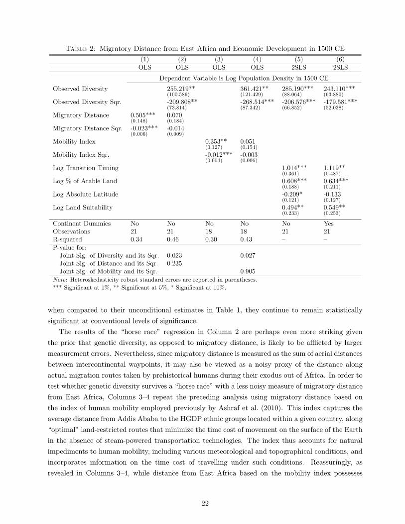
Table 2: Migratory Distance from East Africa and Economic Development in 1500 CE
(1) (2) (3) (4) (5) (6)OLS OLS OLS OLS 2SLS 2SLS
Dependent Variable is Log Population Density in 1500 CE
Observed Diversity 255.219** 361.421** 285.190*** 243.110***(100.586) (121.429) (88.064) (63.880)
Observed Diversity Sqr. -209.808** -268.514*** -206.576*** -179.581***(73.814) (87.342) (66.852) (52.038)
Migratory Distance 0.505*** 0.070(0.148) (0.184)
Migratory Distance Sqr. -0.023*** -0.014(0.006) (0.009)
Mobility Index 0.353** 0.051(0.127) (0.154)
Mobility Index Sqr. -0.012*** -0.003(0.004) (0.006)
Log Transition Timing 1.014*** 1.119**(0.361) (0.487)
Log % of Arable Land 0.608*** 0.634***(0.188) (0.211)
Log Absolute Latitude -0.209* -0.133(0.121) (0.127)
Log Land Suitability 0.494** 0.549**(0.233) (0.253)
Continent Dummies No No No No No YesObservations 21 21 18 18 21 21R-squared 0.34 0.46 0.30 0.43 � �P-value for:Joint Sig. of Diversity and its Sqr. 0.023 0.027Joint Sig. of Distance and its Sqr. 0.235Joint Sig. of Mobility and its Sqr. 0.905
Note : Heteroskedasticity robust standard errors are reported in parentheses.*** Signi�cant at 1%, ** Signi�cant at 5%, * Signi�cant at 10%.
when compared to their unconditional estimates in Table 1, they continue to remain statistically
signi�cant at conventional levels of signi�cance.
The results of the �horse race� regression in Column 2 are perhaps even more striking given
the prior that genetic diversity, as opposed to migratory distance, is likely to be a icted by larger
measurement errors. Nevertheless, since migratory distance is measured as the sum of aerial distances
between intercontinental waypoints, it may also be viewed as a noisy proxy of the distance along
actual migration routes taken by prehistorical humans during their exodus out of Africa. In order to
test whether genetic diversity survives a �horse race�with a less noisy measure of migratory distance
from East Africa, Columns 3�4 repeat the preceding analysis using migratory distance based on
the index of human mobility employed previously by Ashraf et al. (2010). This index captures the
average distance from Addis Ababa to the HGDP ethnic groups located within a given country, along
�optimal�land-restricted routes that minimize the time cost of movement on the surface of the Earth
in the absence of steam-powered transportation technologies. The index thus accounts for natural
impediments to human mobility, including various meteorological and topographical conditions, and
incorporates information on the time cost of travelling under such conditions. Reassuringly, as
revealed in Columns 3�4, while distance from East Africa based on the mobility index possesses
22

a signi�cant hump-shaped correlation with log population density, this unconditional relationship
virtually disappears once genetic diversity is accounted for by the analysis, lending further support
to the claim that distance along prehistorical human migration routes from East Africa confers an
e¤ect on development outcomes through genetic diversity alone.37
The analysis now turns to address concerns regarding the fact that diversity and economic
development may be endogenously determined. In particular, Column 5 presents the results from
estimating the preferred regression speci�cation, with genetic diversity instrumented by migratory
distance.38 The results from a similar analysis that also accounts for continental �xed e¤ects are
reported in Column 6. Interestingly, in comparison to their OLS counterparts in Table 1, the esti-
mated 2SLS coe¢ cients associated with the diversity channel remain relatively stable in magnitude,
suggesting that the potential endogeneity between genetic diversity and economic development need
not be a source of concern, conditional on controls for the transition timing and land productivity
channels. Overall, the results uncovered here provide support for the inferences made with predicted
genetic diversity in the main empirical analysis to follow.
3.2.2 The Baseline Results from the Extended Sample
This section establishes the hump-shaped impact of genetic diversity, predicted by migratory distance
from East Africa, on log population density in 1500 CE, using the extended sample of 145 countries.
To reveal the independent and combined e¤ects of the genetic diversity, transition timing, and
land productivity channels, Table 3 presents the results from estimating a number of speci�cations
spanning relevant subsets of the explanatory variables in equation (8).
The unconditional hump-shaped relationship between genetic diversity and log population density
in 1500 CE is reported in Column 1.39 In particular, the estimated linear and quadratic coe¢ cients,
both statistically signi�cant at the 1% level, imply that a 1 percentage point increase in genetic
diversity for the least diverse society in the regression sample would raise its population density by
59%, whereas a 1 percentage point decrease in genetic diversity for the most diverse society would37The di¤erence in the number of observations between Columns 1�2 (21 obs.) and Columns 3�4 (18 obs.) arises
due to the fact that the mobility index cannot be calculated for countries that can only be accessed from Addis Abababy crossing at least one body of water. Restricting the sample used in Columns 1�2 to that in Columns 3�4 does notqualitatively alter the �ndings. In addition, the unavailability of the mobility index measure for several countries (due tothe aforementioned strict land-accessibility constraint) makes this measure less suitable, in comparison to the baselinemigratory distance measure of Ramachandran et al. (2005), to predict genetic diversity in the extended cross-countrysample. Nevertheless, Table D.5 in Appendix D demonstrates that the main �ndings from both the extended-samplehistorical analysis and the contemporary analysis remain qualitatively robust to using genetic diversity predicted bythe more sophisticated mobility index, rather than by the baseline, waypoints-restricted migratory distance measureof Ramachandran et al. (2005).38Speci�cally, since the empirical speci�cation is quadratic in the endogenous regressor, it is necessary to instrument
for both genetic diversity and its squared term in order for the system to be exactly identi�ed. Thus, followingWooldridge (2010, pp. 267�268), the strategy adopted introduces a zeroth-stage to the analysis where genetic diversityis �rst regressed on migratory distance and all the second-stage controls to obtain predicted values of diversity. Thepredicted genetic diversity from the zeroth-stage is squared and this squared term is then used as an excluded instrumentin the second stage along with migratory distance. The zeroth- and �rst-stage results of the 2SLS regressions reportedin Columns 5 and 6 of Table 2 are collected in Table D.6 in Appendix D.39This quadratic relationship is depicted in Figures C.2(a) and C.2(b) in Appendix C along with a non-parametric
local polynomial regression line and a restricted cubic spline regression line respectively. As in the limited-samplehistorical analysis, the estimated quadratic falls within the 95% con�dence interval bands of both the non-parametricand cubic spline relationships. Footnote 33 provides additional details on the estimation procedures underlying thenon-parametric and cubic spline regressions.
23

Table 3: Predicted Diversity and Economic Development in 1500 CE
(1) (2) (3) (4) (5) (6)
Dependent Variable is Log Population Density in 1500 CE
Predicted Diversity 250.986*** 213.537*** 203.017*** 195.416*** 199.727**(66.314) (61.739) (60.085) (55.916) (80.281)
Predicted Diversity Sqr. -177.399*** -152.107*** -141.980*** -137.977*** -146.167***(48.847) (45.414) (44.157) (40.773) (56.251)
Log Transition Timing 1.287*** 1.047*** 1.160*** 1.235***(0.170) (0.188) (0.143) (0.243)
Log % of Arable Land 0.523*** 0.401*** 0.393***(0.117) (0.096) (0.103)
Log Absolute Latitude -0.167* -0.342*** -0.417***(0.093) (0.096) (0.124)
Log Land Suitability 0.189 0.305*** 0.257***(0.124) (0.094) (0.096)
Optimal Diversity 0.707*** 0.702*** 0.715*** 0.708*** 0.683***(0.021) (0.025) (0.110) (0.051) (0.110)
Continent Dummies No No No No No YesObservations 145 145 145 145 145 145R-squared 0.22 0.26 0.38 0.50 0.67 0.69Note : Bootstrapped standard errors, accounting for the use of generated regressors, are reported in parentheses.*** Signi�cant at 1%, ** Signi�cant at 5%, * Signi�cant at 10%.
raise its population density by 25%.40 Further, population density in 1500 CE is unconditionally
predicted by the regression to be maximized at an expected heterozygosity value of about 0.707,
which roughly corresponds to the diversity predicted (by migratory distance from East Africa) for
southern China. Indeed, a 1 percentage point change in genetic diversity in either direction at the
predicted optimum lowers population density by 1.8%. Moreover, based on the R-squared of the
regression, the cross-country variation in genetic diversity alone explains 22% of the cross-country
variation in population density.
Column 2 reports the unconditional e¤ect of the timing of the agricultural transition on popula-
tion density in 1500 CE. In line with the Diamond hypothesis, a 1% increase in the number of years
elapsed since the Neolithic transition to agriculture is associated with a 1.3% increase in population
density, an e¤ect that is also statistically signi�cant at the 1% level. Furthermore, 26% of the cross-
country variation in population density is explained by the cross-country variation in the timing of
the agricultural transition alone. Perhaps unsurprisingly, as foreshadowed by the sample correlations
in Table G.4 in Appendix G, the unconditional e¤ects of both the genetic diversity and agricultural
transition timing channels are somewhat weakened in magnitude once they are simultaneously taken
into account in Column 3, which reduces the omitted variable bias a icting the coe¢ cient estimates
reported in earlier columns. The coe¢ cients on both channels, however, retain their expected signs
and continue to remain statistically signi�cant at the 1% level with the combined cross-country
variation in genetic diversity and transition timing explaining 38% of the cross-country variation in
population density.
The results of examining the combined explanatory power of the genetic diversity and land
40Following the earlier discussion regarding the expected heterozygosity index, these e¤ects are therefore associatedwith a 0.01 change in the probability that two randomly selected individuals from a given population are geneticallydi¤erent from one another. See Footnote 32 for details on how these e¤ects may be computed based on the estimatedlinear and quadratic coe¢ cients associated with genetic diversity.
24

productivity channels are reported in Column 4.41 Once again, given the sample correlations, the
linear and quadratic coe¢ cients associated with genetic diversity are naturally somewhat weaker
when compared to their unconditional estimates of Column 1. More importantly, the coe¢ cients
remain highly statistically signi�cant and also rather stable in magnitude relative to those estimated
while controlling for the timing of the Neolithic transition. In addition, the overall signi�cance of
the land productivity channel is also con�rmed, particularly by the estimated coe¢ cients on the
log percentage of arable land and log absolute latitude variables, which indeed appear to possess
their expected signs.42 Nonetheless, these estimates continue to re�ect some amount of omitted
variable bias resulting from the exclusion of the transition timing channel. For instance, the fact
that log agricultural transition timing has a sample correlation of 0.28 with genetic diversity and
one of 0.32 with log absolute latitude implies that the estimated e¤ects of these variables on log
population density in Column 4 may be partially capturing the latent in�uence of the excluded
Neolithic transition timing channel.
Column 5 presents the results from exploiting the explanatory power of all three identi�ed
channels for log population density in 1500 CE. In line with the theoretical predictions of each
hypothesis, the coe¢ cient estimates possess their expected signs and are all statistically signi�cant
at the 1% level. Moreover, in comparison to their estimates in Columns 3 and 4, the linear and
quadratic coe¢ cients associated with the diversity channel remain largely stable. In particular, the
estimated coe¢ cients of interest imply that, controlling for the in�uence of land productivity and
the timing of the Neolithic Revolution, a 1 percentage point increase in genetic diversity for the least
diverse society in the sample would raise its population density in 1500 CE by 44%, whereas a 1
percentage point decrease in diversity for the most diverse society would raise its population density
by 18%. Further, population density in 1500 CE is predicted to be maximized at an expected
heterozygosity value of 0.708, where a 1 percentage point change in diversity in either direction
would lower population density by 1.4%. Overall, based on the R-squared of the regression, the
cross-country variations in genetic diversity, agricultural transition timing, and land productivity
together explain 67% of the cross-country variation in population density in 1500 CE.
Finally, Column 6 reports the results from estimating the baseline regression model, speci�ed
in equation (8), which allows the analysis to capture unobserved continent-speci�c attributes that
could potentially have an in�uence on population density. Despite the more modest cross-country
variation in genetic diversity within continents as opposed to that across continents, the coe¢ cients
associated with diversity remain rather stable, increasing slightly in magnitude with the inclusion of
continental dummies, although the statistical signi�cance of the linear coe¢ cient drops to the 5%
level.43 Speci�cally, the coe¢ cients associated with the diversity channel indicate that, controlling
41The cross-country variation in genetic diversity and in variables capturing the productivity of land for agriculturetogether explain 50% of the cross-country variation in population density.42To interpret the coe¢ cients associated with the land productivity channel, a 1% increase in the fraction of arable
land and in absolute latitude corresponds, respectively, to a 0.5% increase and a 0.2% decrease in population density.While this latter e¤ect may seem unintuitive, given the positive relationship between absolute latitude and contemporaryincome per capita, it accurately re�ects the fact that agricultural productivity in the past has typically been higherat latitudinal bands closer to the equator. In addition, this �nding is also consistent with the �reversal of fortune�hypothesis documented by Acemoglu et al. (2005).43Table D.7 in Appendix D demonstrates that the baseline �ndings for genetic diversity from both the limited- and
extended-sample variants of the historical analysis, as well as those from the contemporary analysis, remain qualitatively
25

Figure 4: Predicted Genetic Diversity and Population Density in 1500 CE � Conditional onTransition Timing, Land Productivity, and Continental Fixed E¤ects
for the in�uence of land productivity, the timing of the Neolithic Revolution, and continental �xed
e¤ects, a 1 percentage point increase in diversity for the most homogenous society in the sample would
raise its population density in 1500 CE by 36%, whereas a 1 percentage point decrease in diversity
for the most diverse society would raise its population density by 29%. In addition, a 1 percentage
point change in genetic diversity in either direction at the predicted optimum level of 0.683, which
roughly corresponds to the diversity predicted (by migratory distance from East Africa) for Japan,
would lower population density by 1.5%. Reassuringly, the optimal level of predicted diversity in the
extended sample is quite similar to that obtained for observed diversity in the limited 21-country
sample.
To place the worldwide e¤ect of the diversity channel into perspective, the coe¢ cients reported in
Column 6 imply that increasing the expected heterozygosity of the most homogenous native South
American populations by 11.1 percentage points to the predicted optimum would have raised their
population density in 1500 CE by a factor of 6.07. On the other hand, decreasing the expected
heterozygosity of the most heterogenous East African populations by 9.1 percentage points to the
intact under alternative regression speci�cations that control for some of the individual ecological components of theland suitability index, including temperature, precipitation, and soil fertility, in lieu of the baseline control for theoverall suitability of land for cultivation.In addition, consistent with the fact that the baseline control for the timing of the Neolithic Revolution should be
expected to capture the contemporaneous e¤ect of the mode of subsistence on population density in the pre-colonialMalthusian era, Table D.8 establishes that augmenting the baseline speci�cations for examining population densityin the years 1500 CE and 1000 CE with an explicit control for the mode of subsistence, while diminishing somewhatthe explanatory power of the transition timing channel, does not a¤ect the main �ndings for genetic diversity. Notethat, given underlying data availability constraints on constructing a proxy for the mode of subsistence prevalent inthe year 1500 CE, coupled with the fact that cross-country subsistence patterns in 1000 CE should be expected to behighly correlated with those existing in 1500 CE, the analysis in Table D.8 controls only for the mode of subsistenceprevalent in the year 1000 CE in augmented regressions explaining population density in both time periods. For detailedde�nitions of additional control variables used by the robustness analyses in Tables D.7 and D.8, the interested readeris referred to Appendix F.
26

optimum would have raised their population density by a factor of 3.36. The hump-shaped e¤ect of
genetic diversity on log population density in 1500 CE, conditional on the timing of the Neolithic,
land productivity, and continental �xed e¤ects, is depicted in Figure 4.44 Moreover, the partial
R-squared associated with genetic diversity suggests that residual genetic diversity explains about
7% of the cross-country variation in residual log population density in 1500 CE, conditional on the
covariates from the baseline regression model.
To summarize the results reported in Table 3, genetic diversity as predicted by migratory distance
from East Africa is found to have a highly statistically signi�cant non-monotonic e¤ect on population
density in 1500 CE. This �nding is entirely consistent with the theoretical prediction of the proposed
genetic diversity channel that comprises both an adverse e¤ect of diversity on Malthusian economic
development, via diminished social capital, and a favorable e¤ect arising from increased technological
creativity. The analysis also con�rms the signi�cant bene�cial e¤ects of an earlier Neolithic transition
to agriculture as well as geographical factors conducive to higher agricultural yields. Nevertheless,
controlling for these additional explanatory channels hardly a¤ects the hump-shaped relationship
between genetic diversity and population density, a �nding that remains robust to the inclusion of
continental dummies as well.
3.2.3 Robustness to Aerial Distance and Migratory Distances from �Placebo�Pointsof Origin Across the Globe
The results from the limited sample analysis discussed earlier demonstrate that the cross-country
variation in migratory distance from East Africa has a signi�cant non-monotonic in�uence on com-
parative development in 1500 CE and that this impact runs exclusively via the serial-founder e¤ect on
genetic diversity. This �nding, however, does not preclude the possibility that alternative measures
of distance, potentially correlated with migratory distance from East Africa, may also explain
the historical cross-country variation in economic development in a similar non-monotonic fashion.
Indeed, if this is the case, then the role previously ascribed to the �out of Africa� migration of
Homo sapiens as a deep determinant of comparative development becomes suspect, undermining
the credibility of the proposed genetic diversity channel. Nonetheless, alternative distances, as will
become evident, do not impart any signi�cant in�uence, similar to that associated with migratory
distance from East Africa, on log population density in 1500 CE.
The current analysis compares regression results obtained using migratory distance from Addis
Ababa in the baseline speci�cation with those obtained under several alternative concepts of distance.
The alternative concepts of distance considered by the analysis include the aerial or �as the crow
�ies�distance from Addis Ababa as well as migratory distances from �placebo�points of origin in
other continents across the globe, namely London, Tokyo, and Mexico City, computed using the same
44Figure 4 is an �augmented component plus residual� plot and not the typical �added variable� plot of residualsagainst residuals. In particular, the vertical axis in this �gure represents the component of observed log populationdensity that is predicted by genetic homogeneity and its square plus the residuals from the regression. The horizontalaxis, on the other hand, simply represents genetic homogeneity rather than the residuals obtained from regressinghomogeneity on the covariates. This methodology permits the illustration of the overall non-monotonic e¤ect of thegenetic channel in one scatter plot. Plots depicting the partial regression lines associated with the �rst-order and second-order e¤ects of genetic homogeneity on log population density in 1500 CE are presented in Figures C.3(a)�C.3(b) inAppendix C.
27

Table 4: Robustness to Alternative Distances
(1) (2) (3) (4) (5)Distance from: Addis Ababa Addis Ababa London Tokyo Mexico City
Dependent Variable is Log Population Density in 1500 CE
Migratory Distance 0.138** -0.040 0.052 -0.063(0.061) (0.063) (0.145) (0.099)
Migratory Distance Sqr. -0.008*** -0.002 -0.006 0.005(0.002) (0.002) (0.007) (0.004)
Aerial Distance -0.008(0.106)
Aerial Distance Sqr. -0.005(0.006)
Log Transition Timing 1.160*** 1.158*** 1.003*** 1.047*** 1.619***(0.144) (0.138) (0.164) (0.225) (0.277)
Log % of Arable Land 0.401*** 0.488*** 0.357*** 0.532*** 0.493***(0.091) (0.102) (0.092) (0.089) (0.094)
Log Absolute Latitude -0.342*** -0.263*** -0.358*** -0.334*** -0.239***(0.091) (0.097) (0.112) (0.099) (0.083)
Log Land Suitability 0.305*** 0.254** 0.344*** 0.178** 0.261***(0.091) (0.102) (0.092) (0.080) (0.092)
Observations 145 145 145 145 145R-squared 0.67 0.59 0.67 0.59 0.63Note : Heteroskedasticity robust standard errors are reported in parentheses.*** Signi�cant at 1%, ** Signi�cant at 5%, * Signi�cant at 10%.
waypoints employed in constructing migratory distance from Addis Ababa.45 As revealed in Table
G.4 in Appendix G, with the exception of migratory distance from Tokyo, these other distances
are rather strongly correlated with migratory distance from Addis Ababa. Despite some of these
high correlations, however, the results presented in Table 4 indicate that migratory distance from
Addis Ababa is the only concept of distance that confers a signi�cant non-monotonic e¤ect on log
population density.
Speci�cally, consistent with the proposed diversity hypothesis, Column 1 reveals a highly sta-
tistically signi�cant hump-shaped relationship between migratory distance from Addis Ababa and
log population density in 1500 CE, conditional on controls for the Neolithic transition timing and
land productivity channels. In contrast, the linear and quadratic e¤ects of aerial distance from
Addis Ababa, reported in Column 2, are not statistically di¤erent from zero at conventional levels of
signi�cance. Similarly, as shown in Columns 3�5, the migratory distances from �placebo�points of
origin do not impart any statistically discernible e¤ect, linear or otherwise, on log population density
in the year 1500 CE.
These results strengthen the assertion that conditions innately related to the prehistorical migra-
tion of humans out of Africa have had a lasting impact on comparative development. Given the high
correlations between migratory distance from Addis Ababa and some of these alternative distance
concepts, the fact that these other distances fail to reveal any signi�cant e¤ects makes the argument
in favor of the �out of Africa�hypothesis even stronger. Together with earlier �ndings establishing
45The choice of these alternative points of origin do not re�ect any systematic selection process, other than thecriterion that they belong to di¤erent continents in order to demonstrate, at a global scale, the neutrality of migratorydistance from locations outside of East Africa. Indeed, other points of origin in Europe, Asia and the Americas yieldqualitatively similar results.
28

migratory distance from Addis Ababa and genetic diversity as ultimate and proximate determinants
in the same channel, the �ndings from these �placebo�tests of distance lend further credence to the
proposed diversity hypothesis.
4 The Contemporary Analysis
4.1 Data and Empirical Strategy
This section discusses the data and empirical strategy employed to examine the impact of genetic
diversity on contemporary comparative development.
4.1.1 The Index of Contemporary National Population Diversity
The construction of the index of genetic diversity for contemporary national populations is partly
based on their ethnic compositions resulting from population �ows amongst countries in the post-
Columbian era. Speci�cally, given the genetic diversity of the ancestral populations of the source
countries, data on post-Columbian population �ows can be used to construct a weighted average
expected heterozygosity measure for the national population of each country in the contemporary
period.46 This measure alone, however, would not capture the full extent of genetic diversity in
contemporary national populations as it would fail to account for the diversity arising from di¤erences
between sub-national ethnic groups.
To additionally incorporate the between-group component of diversity in contemporary national
populations, the index makes use of the concept of Fst genetic distance from �eld of population
genetics. Details regarding the construction of this ancestry-adjusted measure of genetic diversity,
that also accounts for the diversity arising from di¤erences between sub-national ethnic groups, are
presented in Appendix B.
Reassuringly, the ancestry-adjusted measure of genetic diversity dominates the unadjusted mea-
sure in predicting economic development in the contemporary period.47 In line with the diversity
hypothesis, Column 1 in Table 5 reveals a signi�cant unconditional hump-shaped relationship between
the adjusted measure of diversity and income per capita in the year 2000 CE.48
Column 2 establishes that the unconditional quadratic relationship from Column 1 remains
qualitatively intact when conditioned for the impact of continent �xed e¤ects. As revealed in
46The data on ethnic compositions are obtained from the World Migration Matrix, 1500�2000 of Putterman andWeil (2010) who compile, for each country in their data set, the share of the country�s population in 2000 CE that isdescended from the population of every other country in 1500 CE.47Table D.9 in Appendix D establishes that migratory distance from Addis Ababa, adjusted to re�ect the weighted
average of migratory distances of the pre-Columbian ancestral populations of a country today, is the only distanceconcept that confers a signi�cant hump-shaped e¤ect on income per capita in 2000 CE. As shown in the table, theother distance concepts, including (i) the unadjusted measure of migratory distance from Addis Ababa (used in thehistorical analysis), (ii) the aerial distance from Addis Ababa, and (iii) the ancestry-adjusted aerial distance fromAddis Ababa, do not confer any systematic non-monotonic e¤ect on income per capita in 2000 CE, given that theancestry-adjusted migratory distance measure is accounted for by the regression.48This quadratic relationship is depicted in Figures C.4(a) and C.4(b) in Appendix C along with a non-parametric
local polynomial regression line and a restricted cubic spline regression line respectively. As in the preceding historicalanalysis, the estimated quadratic falls within the 95% con�dence interval bands of both the non-parametric and cubicspline relationships. Footnote 33 provides additional details on the estimation procedures underlying the non-parametricand cubic spline regressions.
29

Table 5: Adjusted versus Unadjusted Diversity
(1) (2) (3) (4) (5) (6)
Dependent Variable is Log Income Per Capita in 2000 CE
Predicted Diversity 556.439*** 254.906*** 533.983*** 387.314**(Ancestry Adjusted) (129.697) (88.619) (164.216) (188.300)
Predicted Diversity Sqr. -397.224*** -176.907*** -377.365*** -273.925**(Ancestry Adjusted) (90.784) (62.730) (117.645) (136.442)
Predicted Diversity 140.903*** 10.152 1.670 -64.226(Unadjusted) (51.614) (52.732) (69.101) (81.419)
Predicted Diversity Sqr. -107.686*** -7.418 -4.057 51.016(Unadjusted) (38.133) (38.000) (52.990) (64.295)
Continent Dummies No Yes No Yes No YesObservations 143 143 143 143 143 143R-squared 0.13 0.47 0.08 0.45 0.14 0.48P-value for:Joint Sig. of Adjusted Diversity and its Sqr. 0.009 0.038Joint Sig. of Unadjusted Diversity and its Sqr. 0.399 0.741
Note : Bootstrapped standard errors, accounting for the use of generated regressors, are reported in parentheses.*** Signi�cant at 1%, ** Signi�cant at 5%, * Signi�cant at 10%.
Columns 3 and 4, however, while the unadjusted measure also possesses a signi�cant unconditional
hump-shaped relationship with income per capita across countries, the relationship disappears once
the regression is augmented to account for continental dummies. Moreover, examining jointly the
explanatory powers of the ancestry-adjusted and unadjusted measures of genetic diversity for income
per capita, Columns 5 and 6 demonstrate the superior relative performance of the adjusted measure,
regardless of whether continent �xed e¤ects are accounted for, lending further credence ex post to
the methodology employed in constructing the index of contemporary population diversity.
4.1.2 The Empirical Model
Maintaining symmetry with the earlier historical analysis, a regression speci�cation similar to that
employed for the historical regressions is adopted initially to examine the contemporary impact
of genetic diversity along with the transition timing and land productivity channels. The current
speci�cation, however, is further augmented with controls for institutional, cultural, and additional
geographical factors that have received attention in the literature. This permits the examination of
the direct impact of the diversity channel, as opposed to its overall impact that additionally captures
indirect e¤ects potentially correlated with these other determinants.
Formally, the following speci�cation is adopted as a baseline to examine the direct in�uence of
contemporary population diversity on the modern world income distribution:
ln yi = 0 + 1Gi + 2G2i + 3 lnTi +
04 lnXi +
05 ln�i + 6 ln �i + �i, (9)
where yi is the income per capita of country i in the year 2000 CE; Gi is the index of contemporary
population diversity for country i, as discussed above; Ti and Xi are the Neolithic transition timing
and land productivity controls for country i; �i is a vector of institutional and cultural controls for
country i; �i is a vector of additional geographical controls for country i; and, �nally, �i is a country
30

speci�c disturbance term.49
4.2 Empirical Findings
4.2.1 Results for Comparative Development
The empirical �ndings indicate that the highly signi�cant hump-shaped e¤ect of genetic diversity
on macroeconomic outcomes in the pre-industrial period is present in the contemporary period as
well. Furthermore, the persistent hump-shaped impact of genetic diversity on the pattern of com-
parative economic development is a direct e¤ect that is not captured by contemporary geographical,
institutional, and cultural factors.50
Using a sample of 143 countries for which data are available for the entire set of control variables
used in the baseline regression for the year 1500 CE, Column 1 of Table 6 reveals a signi�cant
hump-shaped e¤ect of genetic diversity on income per capita in 2000 CE, accounting for the set of
baseline controls employed in the historical analysis � i.e., the logs of the timing of the Neolithic
transition, the percentage of arable land, absolute latitude and the suitability of land for agriculture,
as well as continental �xed e¤ects.51 Further, consistent with the notion that the optimal level of
diversity increased in the process of industrialization, as the bene�cial forces associated with greater
diversity became intensi�ed in an environment characterized by more rapid technological progress,
the �ndings indicate that the optimal level of diversity with respect to the modern world income
distribution is indeed higher than that obtained with respect to population density in the pre-colonial
Malthusian era. Speci�cally, while the estimate for the optimal level in 1500 CE is 0.683 (Column
4), the estimated optimum in 2000 CE, under the same speci�cation, is 0.713.
Column 2 shows that the hump-shaped e¤ect of diversity on income per capita remains virtually
intact when the control for the Neolithic transition is adjusted to capture the average time elapsed
since the pre-Columbian ancestral populations of each country today experienced the transition
to agriculture (i.e., traits that are embodied in the country�s population today, rather than the
country�s geographical attributes). In particular, the estimated linear and quadratic coe¢ cients on
49The data on income per capita are from the Penn World Table, version 6.2. The institutional and cultural controlsinclude the social infrastructure index of Hall and Jones (1999), the share of the population of European descent basedon the World Migration Matrix, 1500�2000 of Putterman and Weil (2010), legal origin dummies and the shares ofthe population a¢ liated with major world religions from the data set of La Porta et al. (1999), as well as the ethnicfractionalization index of Alesina et al. (2003). The additional geographical controls include the share of the populationat risk of contracting falciparum malaria from Gallup and Sachs (2001), as well as the share of the population livingin Köppen-Geiger tropical zones and distance from the nearest coast or sea-navigable river, both from the data set ofGallup et al. (1999). See Appendix F for further details.50Since (i) genetic diversity for contemporary national populations is partly based on the Fst genetic distances between
their pre-Columbian ancestral groups, and (ii) Fst genetic distances and relative expected heterozygosities, even amongstpopulations in the pre-Columbian era, are in part co-determined by migratory distances, it is necessary to ensure thatthe observed hump-shaped e¤ect of genetic diversity on comparative development, in both the pre-Columbian andcontemporary eras, is not re�ecting the latent impact of genetic distance to either the cradle of humankind or the worldtechnological frontier, via channels related to the di¤usion of development (Spolaore and Wacziarg, 2009). Table D.10in Appendix D demonstrates that the baseline �ndings for genetic diversity from both the limited- and extended-samplevariants of the historical analysis, as well as those from the contemporary analysis, are virtually una¤ected when theregression speci�cations are augmented to account for appropriate measures of Fst genetic distance to Ethiopia andto the world technology frontier relevant for the time period being examined. For detailed de�nitions of the variousgenetic distance controls used by the robustness analysis in Table D.10, the reader is referred to Appendix F.51Tables G.5�G.6 in Appendix G present the relevant descriptive statistics for this 143-country sample.
31

Table 6: Diversity and Economic Development in 2000 CE and 1500 CE
(1) (2) (3) (4)
Dependent Variable is:Log Income Per Capita Log Population Density
in 2000 CE in 1500 CE
Predicted Diversity 204.610** 237.238*** 244.960***(Ancestry Adjusted) (86.385) (85.031) (83.379)
Predicted Diversity Sqr. -143.437** -166.507*** -171.364***(Ancestry Adjusted) (61.088) (60.474) (59.386)
Predicted Diversity 198.587**(Unadjusted) (79.225)
Predicted Diversity Sqr. -145.320***(Unadjusted) (55.438)
Log Transition Timing 0.061 0.002(Ancestry Adjusted) (0.262) (0.305)
Log Transition Timing -0.151 1.238***(Unadjusted) (0.186) (0.241)
Log % of Arable Land -0.110 -0.119 -0.137 0.378***(0.100) (0.107) (0.111) (0.108)
Log Absolute Latitude 0.164 0.172 0.192 -0.423***(0.125) (0.119) (0.143) (0.122)
Log Land Suitability -0.193** -0.177* -0.189* 0.264***(0.095) (0.102) (0.102) (0.095)
Log Population Density in 0.0471500 CE (0.097)
Optimal Diversity 0.713*** 0.712*** 0.715*** 0.683***(0.100) (0.036) (0.118) (0.095)
Continent Dummies Yes Yes Yes YesObservations 143 143 143 143R-squared 0.57 0.57 0.57 0.68Note : Bootstrapped standard errors, accounting for the use of generated regressors, are reported inparentheses.*** Signi�cant at 1%, ** Signi�cant at 5%, * Signi�cant at 10%.
genetic diversity are both statistically signi�cant at the 1% level. They imply that increasing the
diversity of the most genetically homogenous country in the sample (Bolivia) by 1 percentage point
would raise its income per capita in 2000 CE by 29%, whereas decreasing the diversity of the most
genetically diverse country in the sample (Ethiopia) by 1 percentage point would raise its income
per capita by 21%. Further, a 1 percentage point change in diversity (in either direction) at the
optimum level of 0.712 would lower income per capita by 1.7%.52
Importantly, the hump-shaped e¤ect of genetic diversity on income per capita in 2000 CE does
not re�ect an inertia originating from its e¤ect on technology and, thus, population density in 1500
CE. As established in Column 3, the results are essentially unchanged if the regression accounts
for the potentially cofounding e¤ect of population density in 1500 CE. Namely, the e¤ect of genetic
diversity on income per capita in 2000 CE does not operate though its impact on population density
in the year 1500 CE.
The �ndings uncovered by the analysis thus far suggest that genetic diversity has a highly
signi�cant hump-shaped e¤ect on income per capita in the year 2000 CE. Moreover, as established
by the analysis to follow, this overall e¤ect comprises a direct impact that does not operate through
52Table D.13 in Appendix D reports the standardized beta coe¢ cients and partial R-squares associated with eachregressor in the baseline regressions for both the historical and contemporary analyses.
32

institutional, cultural and other geographical factors.
Using a sample of 109 countries for which data are available for the institutional and cultural
controls that are employed in the examination, Column 1 of Table 7 demonstrates that genetic
diversity has a hump-shaped e¤ect on income per capita in the year 2000 CE, accounting for the
set of baseline controls employed in the historical analysis �i.e., the logs of the weighted timing of
the Neolithic transition, the percentage of arable land, and absolute latitude, as well as continental
�xed e¤ects.53 The estimated linear and quadratic coe¢ cients associated with the diversity channel
are both statistically signi�cant at the 1% level and the estimate for the optimal level of diversity
is 0.713. The regression in Column 2 examines the robustness of the results to the inclusion of a
measure of institutional quality, as captured by the social infrastructure index of Hall and Jones
(1999). The estimated hump-shaped e¤ect of genetic diversity remains highly statistically signi�cant
and rather stable, while the optimal level of diversity increases to 0.725.54
The regression in Column 3 is designed to examine whether the e¤ect of genetic diversity operates
via ethnic fractionalization. It demonstrates that the e¤ect of genetic diversity is virtually una¤ected
by the potentially confounding impact of ethnic fractionalization.55 While, as established earlier in
the literature, ethnic fractionalization does indeed confer a signi�cant adverse e¤ect on income per
capita in the year 2000 CE, the hump-shaped impact of genetic diversity remains highly statistically
signi�cant. Moreover, the estimate for the optimal level of diversity, 0.724, is e¤ectively unchanged
in comparison to earlier columns.
Column 4 demonstrates the robustness of the hump-shaped e¤ect of genetic diversity to the
inclusion of additional cultural and institutional controls (i.e., legal origins and the fraction of the
population a¢ liated with major religious). The coe¢ cients associated with genetic diversity remain
highly signi�cant statistically and rather stable in magnitude, while the estimated optimal level of
diversity, 0.722, remains virtually intact.
Column 5 establishes the robustness of the results to the inclusion of controls for the health
environment (i.e., percentage of the population at risk of contracting malaria, and percentage of the
population in tropical zones), additional geographical controls gauging access to waterways, and an
OPEC dummy. The results in this column, which re�ects the baseline speci�cation for examining
the impact of diversity on development in the modern world, therefore reveal the direct e¤ect of
genetic diversity, once institutional, cultural, and geographical factors are accounted for.56 The
53The agricultural suitability index was not found to enter signi�cantly in any of the speci�cations examined in Table7 and is therefore dropped from the analysis. Tables G.7�G.8 in Appendix G present the relevant descriptive statisticsfor the 109-country sample employed in Tables 7�8.54The inclusion of measures from the Polity IV data set, re�ecting the extent of democracy or the degree of constraints
on the power of chief executives, as additional controls for institutional quality do not a¤ect the results for geneticdiversity. Moreover, because these measures enter insigni�cantly in the regression once social infrastructure has beencontrolled for, they are excluded from the analysis in Table 7.55Results (not shown) from estimating a similar speci�cation that included ethnic fractionalization square as an
additional explanatory variable did not reveal any discernible non-monotonic impact of ethnic fractionalization onincome per capita in 2000 CE. Importantly, the regression coe¢ cients associated with genetic diversity, as well as theestimate for the optimal level of diversity, were una¤ected.56As established by Table D.11 in Appendix D, the baseline results for diversity in the contemporary analysis
are qualitatively robust to (i) controls for regional (rather than continental) �xed e¤ects (Column 1), (ii) droppingobservations (Columns 2�4) associated with Sub-Saharan Africa and Latin America that, given their laggarddevelopment in comparison to other regions, along with their relatively higher and lower levels of genetic diversityrespectively, may be considered a priori to be in�uential for generating the worldwide hump-shaped relationship
33

Table7:DiversityandOtherDeterminantsofEconomicDevelopmentin2000CE
(1)
(2)
(3)
(4)
(5)
(6)
(7)
(8)
Full
Full
Full
Full
Full
Full
Schooling
Schooling
Sample
Sample
Sample
Sample
Sample
Sample
Sample
Sample
DependentVariableisLogIncomePerCapitain2000CE
PredictedDiversity
315.282***
225.858***
219.453***
245.377***
277.342***
272.274***
271.249***
215.675***
(AncestryAdjusted)
(85.309)
(67.857)
(67.261)
(69.200)
(69.452)
(83.202)
(73.818)
(67.984)
PredictedDiversitySqr.
-220.980***
-155.826***
-151.489***
-170.036***
-192.386***
-188.868***
-188.899***
-150.871***
(AncestryAdjusted)
(60.304)
(48.011)
(47.512)
(48.737)
(49.056)
(58.239)
(52.806)
(48.295)
LogTransitionTiming
-0.273
-0.092
0.032
0.352
0.396*
0.383
0.112
-0.046
(AncestryAdjusted)
(0.269)
(0.200)
(0.189)
(0.242)
(0.233)
(0.242)
(0.234)
(0.208)
Log%ofArableLand
-0.218***
-0.159***
-0.171***
-0.211***
-0.183***
-0.183***
-0.084
-0.084
(0.061)
(0.049)
(0.049)
(0.047)
(0.051)
(0.051)
(0.056)
(0.056)
LogAbsoluteLatitude
0.123
0.083
0.038
0.119
0.009
0.007
0.007
-0.006
(0.122)
(0.100)
(0.103)
(0.097)
(0.108)
(0.108)
(0.099)
(0.087)
SocialInfrastructure
2.359***
2.389***
2.072***
1.826***
1.810***
1.470***
0.880**
(0.269)
(0.257)
(0.375)
(0.417)
(0.436)
(0.426)
(0.418)
EthnicFractionalization
-0.684**
-0.505
-0.333
-0.336
0.051
-0.122
(0.277)
(0.319)
(0.280)
(0.291)
(0.280)
(0.265)
%ofPopulationatRiskof
-0.502
-0.495
-0.734*
-0.723**
ContractingMalaria
(0.351)
(0.380)
(0.389)
(0.353)
%ofPopulationLivingin
-0.319
-0.312
-0.411*
-0.185
TropicalZones
(0.204)
(0.212)
(0.214)
(0.199)
MeanDistancetoNearest
-0.368**
-0.367*
-0.179
-0.062
Waterway
(0.186)
(0.190)
(0.216)
(0.188)
%ofPopulationofEuropean
0.061
Descent
(0.621)
YearsofSchooling
0.134***
(0.042)
OptimalDiversity
0.713***
0.725***
0.724***
0.722***
0.721***
0.721***
0.718***
0.715***
(0.014)
(0.032)
(0.049)
(0.014)
(0.068)
(0.089)
(0.052)
(0.073)
OPECDummy
No
No
No
No
Yes
Yes
Yes
Yes
LegalOriginDummies
No
No
No
Yes
Yes
Yes
Yes
Yes
MajorReligionShares
No
No
No
Yes
Yes
Yes
Yes
Yes
Observations
109
109
109
109
109
109
9494
R-squared
0.74
0.84
0.85
0.87
0.90
0.90
0.91
0.93
Notes:Bootstrappedstandarderrors,accountingfortheuseofgeneratedregressors,arereportedinparentheses.Allregressionsincludesub-SaharanAfrica
andcontinentdummies.
***Signi�cantat1%,**Signi�cantat5%,*Signi�cantat10%.
34

Figure 5: Adjusted Genetic Diversity and Income Per Capita in 2000 CE � Conditionalon Transition Timing, Land Productivity, Institutional and Geographical Determinants, andContinental Fixed E¤ects
direct hump-shaped impact of genetic diversity on log income per capita in 2000 CE, as established
in Column 5, is depicted in Figure 5.57 Moreover, the partial R-squared associated with genetic
diversity suggests that residual genetic diversity explains about 15% of the cross-country variation in
residual log income per capita in 2000 CE, conditional on the covariates from the baseline regression
model.
The coe¢ cients associated with the diversity channel in Column 5 imply that: (i) increasing the
diversity of the most homogenous country in the sample (Bolivia) by 1 percentage point would raise
its income per capita in the year 2000 CE by 39%, (ii) decreasing the diversity of the most diverse
country in the sample (Ethiopia) by 1 percentage point would raise its income per capita by 21%, (iii)
a 1 percentage point change in genetic diversity (in either direction) at the optimum level of 0.721
(that most closely resembles the diversity level of the U.S.) would lower income per capita by 1.9%,
(iv) increasing the diversity of Bolivia to the level prevalent in the U.S. would increase Bolivia�s per
capita income by a factor of 4.7, closing the income gap between the two countries from a ratio of
12:1 to 2.5:1, and (v) decreasing the diversity of Ethiopia to the level prevalent in the U.S. would
increase Ethiopia�s per capita income by a factor of 1.7 and thus close the income gap between the
two countries from a ratio of 47:1 to 27:1.
The regression in Column 6 examines the robustness of the baseline results to accounting for
the potentially confounding e¤ect of the share of the population of European descent. The results
between diversity and development, and (iii) restricting the regression sample (Column 5) to only countries in thepotentially in�uential Sub-Saharan Africa and Latin America regional clusters. These results demonstrate that thedirect hump-shaped e¤ect of genetic diversity on income per capita in the modern world is not simply a re�ection ofworldwide cross-regional variations in diversity and economic development.57Similar to Figure 4 in the preceding historical analysis, Figure 5 is an �augmented component plus residual�plot
described in detail in Footnote 44. Plots depicting the partial regression lines associated with the �rst-order and second-order e¤ects of genetic homogeneity on log income per capita in 2000 CE are presented in Figures C.5(a)�C.5(b) inAppendix C.
35

Table 8: Addressing Endogenous Post-Columbian Migrations
(1) (2) (3) (4) (5) (6)Full Non w/o Neo w/o Latin w/o Sub >0.97
Sample OECD Europes America Saharan Indigenous
Dependent Variable is Log Income Per Capita in 2000 CE
Predicted Diversity 277.342*** 271.979*** 261.367*** 412.222*** 264.805** 304.735**(Ancestry Adjusted) (69.452) (84.232) (69.946) (148.781) (107.492) (111.588)
Predicted Diversity Sqr. -192.386*** -188.974*** -181.811*** -287.067*** -183.863** -213.389**(Ancestry Adjusted) (49.056) (59.200) (49.261) (102.021) (77.684) (77.255)
Log Transition Timing 0.396* 0.390 0.355 0.518* 0.068 0.448*(Ancestry Adjusted) (0.233) (0.281) (0.231) (0.298) (0.442) (0.254)
Log % of Arable Land -0.183*** -0.236*** -0.201*** -0.189*** -0.211** -0.104(0.051) (0.060) (0.055) (0.050) (0.097) (0.061)
Log Absolute Latitude 0.009 -0.021 -0.025 -0.139 0.218 -0.074(0.108) (0.119) (0.111) (0.126) (0.242) (0.130)
Social Infrastructure 1.826*** 1.313** 1.416*** 2.044*** 1.585*** 1.311*(0.417) (0.579) (0.507) (0.545) (0.486) (0.716)
Ethnic Fractionalization -0.333 -0.437 -0.390 -0.752** 0.104 -0.044(0.280) (0.375) (0.300) (0.348) (0.408) (0.412)
% of Population at Risk -0.502 -0.605 -0.591 -0.308 -0.425 -0.153of Contracting Malaria (0.351) (0.381) (0.370) (0.486) (0.581) (0.434)
% of Population Living -0.319 -0.196 -0.302 -0.520** -0.528 -0.339in Tropical Zones (0.204) (0.239) (0.219) (0.252) (0.341) (0.312)
Mean Distance to -0.368** -0.387* -0.452** -0.494*** -0.743 -0.367*Nearest Waterway (0.186) (0.222) (0.210) (0.186) (0.469) (0.201)
Optimal Diversity 0.721*** 0.720*** 0.719*** 0.718*** 0.720*** 0.714***(0.068) (0.085) (0.015) (0.023) (0.180) (0.012)
Observations 109 83 105 87 71 37R-squared 0.90 0.82 0.89 0.93 0.86 0.98Notes : Bootstrapped standard errors, accounting for the use of generated regressors, are reported in parentheses. Allregressions include controls for major religion shares as well as OPEC, legal origin, sub-Saharan Africa and continentdummies.*** Signi�cant at 1%, ** Signi�cant at 5%, * Signi�cant at 10%.
indicate that the coe¢ cients associated with genetic diversity remain highly statistically signi�cant
and reassuringly stable in magnitude, while the estimated optimal level of diversity is virtually
una¤ected.58
Moreover, as reported in Column 8, even if one accounts for the contribution of human capital
formation over the time period 1960�2000, the hump-shaped e¤ect of genetic diversity on income per
capita in 2000 CE remains highly statistically signi�cant. Further, the estimated optimal level of
diversity drops only moderately from 0.718 (as presented in Column 7, that accounts for the smaller
sample of 94 countries for which data on education and all other variables are available) to 0.715.
Reassuringly, the highly signi�cant and stable hump-shaped e¤ect of genetic diversity on income
per capita in 2000 CE is not an artifact of post-colonial migration towards prosperous countries
and the concomitant increase in ethnic diversity in these economies. Importantly, for the sample of
countries whose national population is largely indigenous to their current geographical location, the
58Since the share of the population of European descent is expected to be highly correlated with unobserved �xede¤ects associated with European countries as well as the Neo-Europes (i.e., USA, Canada, New Zealand, and Australia),Table D.12 in Appendix D repeats the analysis from Columns 5�6 in Table 7 on di¤erent cuts of the cross-countrysample, focusing primarily on countries where the share of Europeans in the population is not confoundingly close to 1.Importantly, the �ndings therein suggest that the baseline results are robust to controlling for the share of Europeans inthe population even when the sample is restricted to non-OECD countries (Columns 3�4), non Neo-European countries(Columns 5�6), and non-European countries (Columns 7�8).
36

hump-shaped e¤ect of genetic diversity on contemporary income per capita is highly signi�cant and
virtually identical to the one observed in the entire sample. Thus, since genetic diversity in these
populations is the level of diversity predicted by migratory distance from East Africa, rather than
the actual one, the potential concern about endogeneity between genetic diversity and income per
capita in the modern world is alleviated.
In particular, as established in Table 8, the hump-shaped e¤ect of genetic diversity remains highly
signi�cant and the optimal diversity estimate remains virtually intact if the sample is restricted to
(a) non-OECD economies (i.e., economies that were less attractive to migrants) in Column 2, (b)
non Neo-European countries (i.e., excluding USA, Canada, New Zealand and Australia) in Column
3, (c) non-Latin American countries in Column 4, (d) non Sub-Saharan African countries in Column
5, and (e) countries whose indigenous population is larger than 97% of the entire population (i.e.,
under conditions that virtually eliminate the role of migration in the creation of diversity over the
last 500 years) in Column 6.59
4.2.2 The Costs and Bene�ts of Genetic Diversity
This section presents empirical evidence on some of the channels through which genetic diversity
confers a hump-shaped e¤ect on income per capita across countries in the modern world. In line with
the theory that diversity should be expected to confer costs on productivity, in the form of lower social
capital, and bene�ts, in the form of more rapid knowledge creation, it establishes that countries with
greater diversity are also characterized, on average, by a lower prevalence of interpersonal trust and
a higher intensity of scienti�c knowledge creation. Speci�cally, exploiting cross-country variations in
the degree of interpersonal trust and the annual average number of scienti�c articles per capita in the
1981�2000 time period, the analysis demonstrates that genetic diversity has a statistically signi�cant
negative relationship with the prevalence of trust but a positive one with scienti�c productivity,
conditional on a similar set of baseline controls employed in the preceding analysis of contemporary
comparative development.60
Using a sample of 58 countries for which trust data as well as data on all baseline controls employed
by the analysis are available, Column 1 of Table 9 shows that genetic diversity has a statistically
signi�cant negative e¤ect on the prevalence of trust, accounting for the Neolithic transition timing
and land productivity channels, as well as contemporary cultural, geographical, and institutional
factors. The coe¢ cient corresponding to the diversity channel indicates that a 1 percentage point
increase in genetic diversity is associated with a 0.02 percentage point decrease in the prevalence of
trust. Moreover, as demonstrated in Column 2, this adverse impact of diversity on trust remains
59This result re�ects the well-known fact from the �eld of population genetics that the overwhelming majority ofgenetic diversity in human populations stems from the diversity within groups, as opposed to the diversity betweengroups (see, e.g., Barbujani et al., 1997).60Consistently with empirical �ndings in the existing literature, Table D.14 in Appendix D demonstrates that the
prevalence of trust and the intensity of scienti�c knowledge creation both individually possess statistically signi�cantpositive correlations with log income per capita in 2000 CE. These correlations hold both unconditionally (Columns 1and 4) and conditional on either the baseline set of controls from the historical analysis (Columns 2 and 5) or a morecomprehensive set of institutional, cultural, and geographical controls from the contemporary analysis (Columns 3 and6). For details on the de�nitions and data sources of the variables gauging the prevalence of trust and the intensity ofscienti�c knowledge creation, the reader is referred to Appendix F.
37

Table 9: The Costs and Bene�ts of Diversity
(1) (2) (3) (4) (5) (6)Full Full Common Full Full Common
Sample Sample Sample Sample Sample Sample
Dependent Variable is:
Degree of Scienti�c ArticlesInterpersonal per Capita per Year
Trust 1981-2000
Predicted Diversity -1.855** -2.193** -1.901** 2.371*** 1.761*** 2.816**(Ancestry Adjusted) (0.861) (0.873) (0.937) (0.558) (0.530) (1.233)
Log Transition Timing 0.069 0.079 0.083 -0.087* -0.080* -0.180**(Ancestry Adjusted) (0.068) (0.067) (0.063) (0.046) (0.045) (0.086)
Log % of Arable Land 0.002 -0.004 -0.017 0.009 0.006 -0.004(0.020) (0.018) (0.018) (0.016) (0.015) (0.037)
Log Absolute Latitude -0.006 0.017 0.009 0.046* 0.055** 0.078(0.029) (0.029) (0.030) (0.024) (0.023) (0.072)
Social Infrastructure 0.201*** 0.108 0.102 0.697*** 0.542*** 0.627***(0.070) (0.085) (0.083) (0.109) (0.124) (0.200)
Ethnic Fractionalization 0.056 0.053 0.062 0.093 0.075 0.089(0.071) (0.066) (0.070) (0.095) (0.094) (0.156)
% of Population at Risk -0.062 -0.022 -0.038 0.095* 0.136*** 0.026of Contracting Malaria (0.090) (0.088) (0.093) (0.054) (0.048) (0.121)
% of Population Living -0.076 0.002 0.006 0.016 0.049 0.108in Tropical Zones (0.055) (0.064) (0.063) (0.058) (0.055) (0.181)
Mean Distance to 0.093 0.115* 0.096* 0.106*** 0.117*** 0.159**Nearest Waterway (0.061) (0.059) (0.055) (0.038) (0.034) (0.067)
Years of Schooling 0.021* 0.027** 0.031*** 0.021(0.012) (0.011) (0.008) (0.023)
Observations 58 58 56 93 93 56R-squared 0.79 0.80 0.82 0.80 0.82 0.81Notes : Bootstrapped standard errors, accounting for the use of a generated regressor, are reported inparentheses. All regressions include additional geographical controls for terrain characteristics, as wellas OPEC, legal origin, sub-Saharan Africa and continent dummies.*** Signi�cant at 1%, ** Signi�cant at 5%, * Signi�cant at 10%.
intact when the regression speci�cation is augmented to account for the e¤ect of average years of
schooling in the population.
In contrast, using a sample of 93 countries for which data on scienti�c productivity as well as
data on the full set of baseline controls are available, Column 4 shows that genetic diversity has a
statistically signi�cant positive e¤ect on the average annual number of published scienti�c articles per
capita. Speci�cally, the coe¢ cient of interest indicates that a 1 percentage point increase in genetic
diversity is associated with an increase in the annual number of scienti�c articles per capita of about
0.02, conditional on the in�uence of Neolithic transition timing, land productivity, and contemporary
cultural, geographical, and institutional factors. In addition, as established by Column 5, accounting
for the e¤ect of average years of schooling in the population does not qualitatively alter the bene�cial
impact of diversity on scienti�c productivity in the 1981�2000 time period.
Finally, Columns 3 and 6 demonstrate that the conditional detrimental e¤ect of genetic diversity
on trust as well as its bene�cial e¤ect on scienti�c productivity both remain fully intact when the
relevant regressions are performed on a common sample of countries, thereby lending further support
to the theoretical assertion that diversity confers con�icting e¤ects on productivity, generating
ine¢ ciencies in the production process while, at the same time, fostering the expansion of society�s
38

production possibility frontier.
5 Concluding Remarks
This paper argues that deep-rooted factors, determined tens of thousands of years ago, had a
signi�cant e¤ect on the course of economic development from the dawn of human civilization to the
contemporary era. It advances and empirically establishes the hypothesis that, in the course of the
exodus of Homo sapiens out of Africa, variation in migratory distance from the cradle of humankind
to various settlements across the globe a¤ected genetic diversity, and has had a long-lasting e¤ect on
the pattern of comparative economic development that is not captured by geographical, institutional,
and cultural factors.
The level of genetic diversity within a society is found to have a hump-shaped e¤ect on de-
velopment outcomes in the pre-colonial era, re�ecting the trade-o¤ between the bene�cial and the
detrimental e¤ects of diversity on productivity. Moreover, the level of genetic diversity in each
country today (as determined by the genetic diversities and genetic distances amongst its ancestral
populations), has a non-monotonic e¤ect on income per capita in the modern world. While the
intermediate level of genetic diversity prevalent among Asian and European populations has been
conducive for development, the high degree of diversity among African populations and the low degree
of diversity among Native American populations have been a detrimental force in the development
of these regions.
References
Acemoglu, Daron, Simon Johnson, and James A. Robinson, �Institutions as a FundamentalCause of Long-Run Growth,� in Philippe Aghion and Steven N. Durlauf, eds., Handbook of
Economic Growth, Vol IA, Amsterdam, The Netherlands: Elsevier North-Holland, 2005.
Alesina, Alberto and Eliana La Ferrara, �Ethnic Diversity and Economic Performance,�Journalof Economic Literature, September 2005, 43 (3), 762�800.
, Arnaud Devleeschauwer, William Easterly, Sergio Kurlat, and Romain Wacziarg,�Fractionalization,�Journal of Economic Growth, June 2003, 8 (2), 155�194.
Ashraf, Quamrul and Oded Galor, �Dynamics and Stagnation in the Malthusian Epoch,�American Economic Review, August 2011, 101 (5), 2003�2041.
, , and Ömer Özak, �Isolation and Development,� Journal of the European EconomicAssociation, April-May 2010, 8 (2-3), 401�412.
Bairoch, Paul, Cities and Economic Development: From the Dawn of History to the Present,
Trans. by Christopher Braider. Chicago, IL: The University of Chicago Press, 1988.
Barbujani, Guido, Arianna Magagni, Eric Minch, and L. Luca Cavalli-Sforza, �AnApportionment of Human DNA Diversity,�Proceedings of the National Academy of Sciences,
April 1997, 94 (9), 4516�4519.
Barro, Robert J. and Rachel M. McCleary, �Religion and Economic Growth across Countries,�American Sociological Review, October 2003, 68 (5), 760�781.
39

Cann, Howard M., Claudia de Toma, Lucien Cazes, Marie-Fernande Legrand, ValerieMorel, Laurence Piou¤re et al., �A Human Genome Diversity Cell Line Panel,� Science,
April 2002, 296 (5566), 261�262.
Cavalli-Sforza, L. Luca, �The Human Genome Diversity Project: Past, Present and Future,�Nature Reviews Genetics, April 2005, 6 (4), 333�340.
Conley, Timothy G., �GMM Estimation with Cross Sectional Dependence,� Journal of
Econometrics, September 1999, 92 (1), 1�45.
Dalgaard, Carl-Johan and Holger Strulik, �The Physiological Foundations of the Wealth ofNations,�2010. Discussion Paper No. 10-05, University of Copenhagen.
Desmet, Klaus, Michel Le Breton, Ignacio Ortuño-Ortín, and Shlomo Weber, �TheStability and Breakup of Nations: A Quantitative Analysis,� Journal of Economic Growth,
September 2011, 16 (3), 183�213.
Diamond, Jared, Guns, Germs and Steel: The Fates of Human Societies, New York, NY: W. W.Norton & Co., 1997.
, �Evolution, Consequences and Future of Plant and Animal Domestication,�Nature, August
2002, 418 (6898), 700�707.
Easterly, William and Ross Levine, �Africa�s Growth Tragedy: Policies and Ethnic Divisions,�Quarterly Journal of Economics, November 1997, 112 (4), 1203�1250.
Engerman, Stanley L. and Kenneth L. Sokolo¤, �History Lessons: Institutions, Factor
Endowments, and Paths of Development in the New World,�Journal of Economic Perspectives,
Summer 2000, 14 (3), 217�232.
Gallup, John L. and Je¤rey D. Sachs, �The Economic Burden of Malaria,� The AmericanJournal of Tropical Medicine and Hygiene, January 2001, 64 (1-2), 85�96.
, , and Andrew D. Mellinger, �Geography and Economic Development,�InternationalRegional Science Review, August 1999, 22 (2), 179�232.
Galor, Oded, Uni�ed Growth Theory, Princeton, NJ: Princeton University Press, 2011.and Omer Moav, �Natural Selection and the Origin of Economic Growth,�Quarterly Journalof Economics, November 2002, 117 (4), 1133�1191.
and , �The Neolithic Revolution and Contemporary Variations in Life Expectancy,�2007.
Working Paper, Department of Economics, Brown University.
and Stelios Michalopoulos, �Evolution and the Growth Process: Natural Selection ofEntrepreneurial Traits,�2011. Journal of Economic Theory, forthcoming.
Glaeser, Edward L., Rafael La Porta, Florencio Lopez-de-Silanes, and Andrei Shleifer,�Do Institutions Cause Growth?,� Journal of Economic Growth, September 2004, 9 (3), 271�
303.
Greif, Avner, �Contract Enforceability and Economic Institutions in Early Trade: The MaghribiTraders�Coalition,�American Economic Review, June 1993, 83 (3), 525�548.
Gri¢ ths, Anthony J. F., Je¤rey H. Miller, David T. Suzuki, Richard C. Lewontin, andWilliam M. Gelbart, An Introduction to Genetic Analysis, New York, NY: W. H. Freeman& Co., 2000.
Guiso, Luigi, Paola Sapienza, and Luigi Zingales, �Cultural Biases in Economic Exchange?,�
40

Quarterly Journal of Economics, August 2009, 124 (3), 1095�1131.
Hall, Robert E. and Charles I. Jones, �Why Do Some Countries Produce So Much More OutputPer Worker Than Others?,�Quarterly Journal of Economics, February 1999, 114 (1), 83�116.
Jones, Eric L., The European Miracle: Environments, Economies and Geopolitics in the Historyof Europe and Asia, Cambridge, UK: Cambridge University Press, 1981.
La Porta, Rafael, Florencio Lopez-de-Silanes, Andrei Shleifer, and Robert W. Vishny,�The Quality of Government,�Journal of Law, Economics, and Organization, March 1999, 15
(1), 222�279.
Lagerlöf, Nils-Petter, �Long-Run Trends in Human Body Mass,�Macroeconomic Dynamics, June2007, 11 (3), 367�387.
Landes, David S., The Wealth and Poverty of Nations: Why Some Are So Rich and Some SoPoor, New York, NY: W. W. Norton & Co., 1998.
Macaulay, Vincent, Catherine Hill, Alessandro Achilli, Chiara Rengo, Douglas Clarke,William Meehan et al., �Single, Rapid Coastal Settlement of Asia Revealed by Analysis ofComplete Mitochondrial Genomes,�Science, May 2005, 308 (5724), 1034�1036.
McEvedy, Colin and Richard Jones, Atlas of World Population History, New York, NY: PenguinBooks Ltd., 1978.
Michalopoulos, Stelios, �The Origins of Ethnolinguistic Diversity,� 2011. American EconomicReview, forthcoming.
Mokyr, Joel, The Lever of Riches: Technological Creativity and Economic Progress, New York,
NY: Oxford University Press, 1990.
Murphy, Kevin M. and Robert H. Topel, �Estimation and Inference in Two-Step EconometricModels,�Journal of Business and Economic Statistics, October 1985, 3 (4), 370�379.
North, Douglass C. and Robert P. Thomas, The Rise of the Western World: A New EconomicHistory, Cambridge, UK: Cambridge University Press, 1973.
Olsson, Ola and Douglas A. Hibbs Jr., �Biogeography and Long-Run Economic Development,�European Economic Review, May 2005, 49 (4), 909�938.
Pagan, Adrian, �Econometric Issues in the Analysis of Regressions with Generated Regressors,�International Economic Review, February 1984, 25 (1), 221�247.
Pomeranz, Kenneth, The Great Divergence: Europe, China and the Making of the Modern WorldEconomy, Princeton, NJ: Princeton University Press, 2000.
Prugnolle, Franck, Andrea Manica, and François Balloux, �Geography Predicts NeutralGenetic Diversity of Human Populations,�Current Biology, March 2005, 15 (5), R159�R160.
Putterman, Louis, �Agriculture, Di¤usion, and Development: Ripple E¤ects of the NeolithicRevolution,�Economica, November 2008, 75 (300), 729�748.
and David N. Weil, �Post-1500 Population Flows and the Long Run Determinants ofEconomic Growth and Inequality,�Quarterly Journal of Economics, November 2010, 125 (4),
1627�1682.
Ramachandran, Sohini, Omkar Deshpande, Charles C. Roseman, Noah A. Rosenberg,Marcus W. Feldman, and L. Luca Cavalli-Sforza, �Support from the Relationship of
Genetic and Geographic Distance in Human Populations for a Serial Founder E¤ect Originating
41

in Africa,�Proceedings of the National Academy of Sciences, November 2005, 102 (44), 15942�
15947.
Ramankutty, Navin, Jonathan A. Foley, John Norman, and Kevin McSweeney, �TheGlobal Distribution of Cultivable Lands: Current Patterns and Sensitivity to Possible Climate
Change,�Global Ecology and Biogeography, September 2002, 11 (5), 377�392.
Robinson, Gene E. and Robert E. Page Jr., �The Genetic Basis of Division of Labor in anInsect Society,� in Michael D. Breed and Robert E. Page, Jr., eds., The Genetics of Social
Evolution, Boulder, CO: Westview Press, 1989.
Rodrik, Dani, Arvind Subramanian, and Francesco Trebbi, �Institutions Rule: The
Primacy of Institutions Over Geography and Integration in Economic Development,� Journal
of Economic Growth, June 2004, 9 (2), 131�165.
Spolaore, Enrico and Romain Wacziarg, �The Di¤usion of Development,�Quarterly Journalof Economics, May 2009, 124 (2), 469�529.
Stringer, Chris B. and Peter Andrews, �Genetic and Fossil Evidence for the Origin of ModernHumans,�Science, March 1988, 239 (4845), 1263�1268.
Tabellini, Guido, �Institutions and Culture,� Journal of the European Economic Association,April-May 2008, 6 (2-3), 255�294.
Wang, Sijia, Cecil M. Lewis Jr., Mattias Jakobsson, Sohini Ramachandran, Nicolas Ray,Gabriel Bedoya et al., �Genetic Variation and Population Structure in Native Americans,�PLoS Genetics, November 2007, 3 (11), 2049�2067.
Weber, Max, The Protestant Ethic and the Spirit of Capitalism, Trans. by Talcott Parsons andAnthony Giddens, 1930. London, UK: Allen & Unwin, 1905.
Wooldridge, Je¤rey M., Econometric Analysis of Cross Section and Panel Data, 2 ed., Cambridge,MA: The MIT Press, 2010.
42

Appendices (For Online Publication)
A Additional Robustness Checks
A.1 Results for Earlier Historical Periods
This section examines the e¤ects of genetic diversity on economic development in earlier historicalperiods of the Common Era and, in particular, establishes a hump-shaped relationship betweengenetic diversity, predicted by migratory distance from East Africa, and log population density inthe years 1000 CE and 1 CE. In so doing, the analysis demonstrates the persistence of the diversitychannel over a long expanse of time and indicates that the hump-shaped manner in which geneticdiversity in�uences development, along with the optimal level of diversity, did not fundamentallychange during the agricultural stage of development.
The results from replicating the analysis of the previous section to explain log population densityin 1000 CE and 1 CE are presented in Tables A.1 and A.2 respectively. As before, the individualand combined explanatory powers of the genetic diversity, transition timing, and land productivitychannels are examined empirically. The relevant samples, determined by the availability of data onthe dependent variable of interest as well as all identi�ed explanatory channels, are comprised of 140countries for the 1000 CE regressions and 126 countries for the analysis in 1 CE. Despite the moreconstrained sample sizes, however, the empirical �ndings once again reveal a highly statisticallysigni�cant hump-shaped relationship between genetic diversity, predicted by migratory distancefrom East Africa, and log population density in these earlier historical periods. Additionally, themagnitude and signi�cance of the coe¢ cients associated with the diversity channel in these earlierperiods remain rather stable, albeit less so in comparison to the analysis for 1500 CE, when theregression speci�cation is augmented with controls for the transition timing and land productivitychannels as well as dummy variables capturing continental �xed e¤ects.
In a pattern similar to that observed in Table 3, the unconditional e¤ects of genetic diversityin Tables A.1 and A.2 decrease slightly in magnitude when subjected to controls for either theNeolithic transition timing or the land productivity channels, both of which appear to confer theirexpected e¤ects on population density in earlier historical periods. However, as argued previously,these estimates certainly re�ect some amount of omitted variable bias resulting from the exclusionof one or more of the identi�ed explanatory channels in Malthusian economic development. Onthe other hand, unlike the pattern in Table 3, the coe¢ cients of the diversity channel also weakenmoderately in statistical signi�cance, dropping to the 5% level when controlling for transition timingin the 1000 CE analysis and to the 10% level under controls for the land productivity channel in the 1CE analysis. Nonetheless, this reduction in signi�cance is not entirely surprising when one accountsfor the greater imprecision with which population density is recorded for these earlier periods, giventhat mismeasurement in the dependent variable of an OLS regression typically causes the resultingcoe¢ cient estimates to possess larger standard errors.
Column 5 in Tables A.1 and A.2 reveals the results from exploiting the combined explanatorypower of the genetic diversity, transition timing, and land productivity channels for log populationdensity in 1000 CE and 1 CE. Interestingly, in each case, the linear and quadratic coe¢ cients asso-ciated with diversity remain rather stable when compared to the corresponding estimates obtainedunder a partial set of controls in earlier columns. In comparison to the corresponding results forpopulation density in 1500 CE from Table 3, the coe¢ cients of the diversity channel uncoveredhere are statistically signi�cant at the 5% as opposed to the 1% level, a by-product of relativelylarger standard errors that again may be partly attributed to the higher measurement error a ictingpopulation density estimates reported for earlier historical periods.
Finally, the last column in each table augments the analysis with controls for continental �xed
i

Figure A.1: Predicted Genetic Diversity and Population Density in 1000 CE �Conditional onTransition Timing, Land Productivity, and Continental Fixed E¤ects
Figure A.2: Predicted Genetic Diversity and Population Density in 1 CE � Conditional onTransition Timing, Land Productivity, and Continental Fixed E¤ects
ii
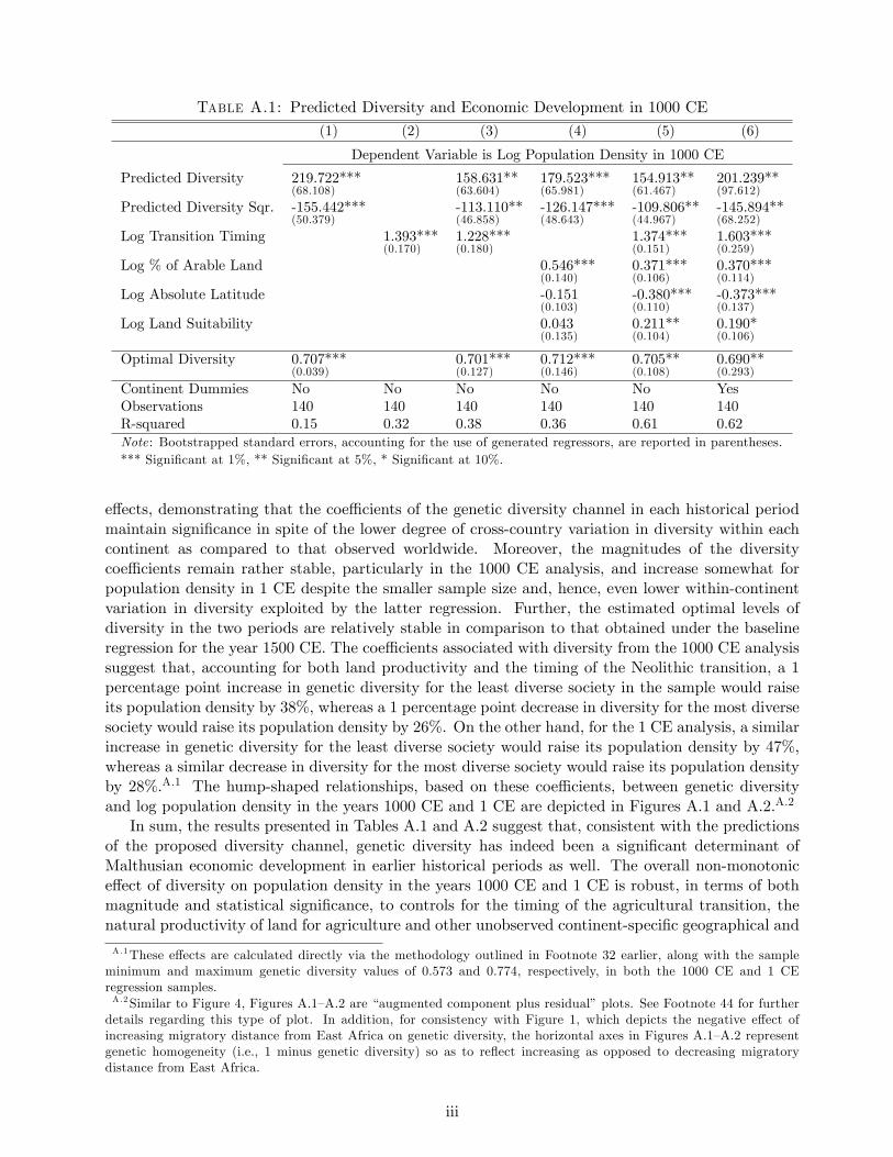
Table A.1: Predicted Diversity and Economic Development in 1000 CE
(1) (2) (3) (4) (5) (6)
Dependent Variable is Log Population Density in 1000 CE
Predicted Diversity 219.722*** 158.631** 179.523*** 154.913** 201.239**(68.108) (63.604) (65.981) (61.467) (97.612)
Predicted Diversity Sqr. -155.442*** -113.110** -126.147*** -109.806** -145.894**(50.379) (46.858) (48.643) (44.967) (68.252)
Log Transition Timing 1.393*** 1.228*** 1.374*** 1.603***(0.170) (0.180) (0.151) (0.259)
Log % of Arable Land 0.546*** 0.371*** 0.370***(0.140) (0.106) (0.114)
Log Absolute Latitude -0.151 -0.380*** -0.373***(0.103) (0.110) (0.137)
Log Land Suitability 0.043 0.211** 0.190*(0.135) (0.104) (0.106)
Optimal Diversity 0.707*** 0.701*** 0.712*** 0.705** 0.690**(0.039) (0.127) (0.146) (0.108) (0.293)
Continent Dummies No No No No No YesObservations 140 140 140 140 140 140R-squared 0.15 0.32 0.38 0.36 0.61 0.62Note : Bootstrapped standard errors, accounting for the use of generated regressors, are reported in parentheses.*** Signi�cant at 1%, ** Signi�cant at 5%, * Signi�cant at 10%.
e¤ects, demonstrating that the coe¢ cients of the genetic diversity channel in each historical periodmaintain signi�cance in spite of the lower degree of cross-country variation in diversity within eachcontinent as compared to that observed worldwide. Moreover, the magnitudes of the diversitycoe¢ cients remain rather stable, particularly in the 1000 CE analysis, and increase somewhat forpopulation density in 1 CE despite the smaller sample size and, hence, even lower within-continentvariation in diversity exploited by the latter regression. Further, the estimated optimal levels ofdiversity in the two periods are relatively stable in comparison to that obtained under the baselineregression for the year 1500 CE. The coe¢ cients associated with diversity from the 1000 CE analysissuggest that, accounting for both land productivity and the timing of the Neolithic transition, a 1percentage point increase in genetic diversity for the least diverse society in the sample would raiseits population density by 38%, whereas a 1 percentage point decrease in diversity for the most diversesociety would raise its population density by 26%. On the other hand, for the 1 CE analysis, a similarincrease in genetic diversity for the least diverse society would raise its population density by 47%,whereas a similar decrease in diversity for the most diverse society would raise its population densityby 28%.A.1 The hump-shaped relationships, based on these coe¢ cients, between genetic diversityand log population density in the years 1000 CE and 1 CE are depicted in Figures A.1 and A.2.A.2
In sum, the results presented in Tables A.1 and A.2 suggest that, consistent with the predictionsof the proposed diversity channel, genetic diversity has indeed been a signi�cant determinant ofMalthusian economic development in earlier historical periods as well. The overall non-monotonice¤ect of diversity on population density in the years 1000 CE and 1 CE is robust, in terms of bothmagnitude and statistical signi�cance, to controls for the timing of the agricultural transition, thenatural productivity of land for agriculture and other unobserved continent-speci�c geographical and
A.1These e¤ects are calculated directly via the methodology outlined in Footnote 32 earlier, along with the sampleminimum and maximum genetic diversity values of 0.573 and 0.774, respectively, in both the 1000 CE and 1 CEregression samples.A.2Similar to Figure 4, Figures A.1�A.2 are �augmented component plus residual�plots. See Footnote 44 for furtherdetails regarding this type of plot. In addition, for consistency with Figure 1, which depicts the negative e¤ect ofincreasing migratory distance from East Africa on genetic diversity, the horizontal axes in Figures A.1�A.2 representgenetic homogeneity (i.e., 1 minus genetic diversity) so as to re�ect increasing as opposed to decreasing migratorydistance from East Africa.
iii

Table A.2: Predicted Diversity and Economic Development in 1 CE
(1) (2) (3) (4) (5) (6)
Dependent Variable is Log Population Density in 1 CE
Predicted Diversity 227.826*** 183.142*** 129.180* 134.767** 231.689**(72.281) (57.772) (66.952) (59.772) (113.162)
Predicted Diversity Sqr. -160.351*** -132.373*** -88.040* -96.253** -166.859**(53.169) (42.177) (49.519) (43.718) (79.175)
Log Transition Timing 1.793*** 1.636*** 1.662*** 2.127***(0.217) (0.207) (0.209) (0.430)
Log % of Arable Land 0.377** 0.314** 0.348***(0.158) (0.125) (0.134)
Log Absolute Latitude 0.190 -0.121 -0.115(0.125) (0.119) (0.135)
Log Land Suitability 0.160 0.238* 0.210*(0.173) (0.124) (0.125)
Optimal Diversity 0.710*** 0.692*** 0.734** 0.700*** 0.694***(0.052) (0.027) (0.347) (0.188) (0.194)
Continent Dummies No No No No No YesObservations 126 126 126 126 126 126R-squared 0.16 0.42 0.46 0.32 0.59 0.61Note : Bootstrapped standard errors, accounting for the use of generated regressors, are reported in parentheses.*** Signi�cant at 1%, ** Signi�cant at 5%, * Signi�cant at 10%.
socioeconomic characteristics. More fundamentally, the analysis demonstrates the persistence of thediversity channel, along with the optimal level of diversity, over a long expanse of time during theagricultural stage of development.
A.2 Robustness to the Technology Di¤usion Hypothesis
The technology di¤usion hypothesis, as mentioned earlier, suggests that spatial proximity to globaland regional technological frontiers confers a bene�cial e¤ect on the development of less advancedsocieties by facilitating the di¤usion of new technologies from more advanced societies throughtrade as well as sociocultural and geopolitical in�uences. In particular, the technology di¤usionchannel implies that, ceteris paribus, the greater the geographic distance from the global and regionaltechnological �leaders� in a given period, the lower the level of economic development amongst the�followers� in that period. Indeed, several studies in international trade and economic geographyhave uncovered strong empirical support for this hypothesis in explaining comparative economicdevelopment in the contemporary era. This section examines the robustness of the e¤ects of ge-netic diversity on economic development during the pre-colonial era to controls for this additionalhypothesis.
The purpose of the current investigation is to ensure that the preceding analyses were not ascribingto genetic diversity the predictive power that should otherwise have been attributed to the technologydi¤usion channel. To be speci�c, one may identify some of the waypoints employed to construct theprehistorical migratory routes from East Africa (such as Cairo and Istanbul) as origins of spatialtechnology di¤usion during the pre-colonial era. This, coupled with the fact that genetic diversitydecreases with increasing migratory distance from East Africa, raises the concern that what hasso far been interpreted as evidence consistent with the bene�cial e¤ect of higher diversity may, inreality, simply be capturing the latent e¤ect of the omitted technology di¤usion channel in precedingregression speci�cations. As will become evident, however, while technology di¤usion is indeedfound to have been a signi�cant determinant of comparative development in the pre-colonial era,the baseline �ndings for genetic diversity remain robust to controls for this additional in�uentialhypothesis.
iv

Table A.3: The Regional Frontiers Identi�ed for each Historical Period
City and Modern Location Continent Sociopolitical Entity Relevant PeriodCairo, Egypt Africa Mamluk Sultanate 1500 CEFez, Morocco Africa Marinid Kingdom of Fez 1500 CELondon, UK Europe Tudor Dynasty 1500 CEParis, France Europe Valois-Orléans Dynasty 1500 CEConstantinople, Turkey Asia Ottoman Empire 1500 CEPeking, China Asia Ming Dynasty 1500 CETenochtitlan, Mexico Americas Aztec Civilization 1500 CECuzco, Peru Americas Inca Civilization 1500 CECairo, Egypt Africa Fatimid Caliphate 1000 CEKairwan, Tunisia Africa Berber Zirite Dynasty 1000 CEConstantinople, Turkey Europe Byzantine Empire 1000 CECordoba, Spain Europe Caliphate of Cordoba 1000 CEBaghdad, Iraq Asia Abbasid Caliphate 1000 CEKaifeng, China Asia Song Dynasty 1000 CETollan, Mexico Americas Classic Maya Civilization 1000 CEHuari, Peru Americas Huari Culture 1000 CEAlexandria, Egypt Africa Roman Empire 1 CECarthage, Tunisia Africa Roman Empire 1 CEAthens, Greece Europe Roman Empire 1 CERome, Italy Europe Roman Empire 1 CELuoyang, China Asia Han Dynasty 1 CESeleucia, Iraq Asia Seleucid Dynasty 1 CETeotihuacán, Mexico Americas Pre-classic Maya Civilization 1 CECahuachi, Peru Americas Nazca Culture 1 CE
To account for the technology di¤usion channel, the current analysis constructs, for each his-torical period examined, a control variable measuring the great circle distance from the closestregional technological frontier in that period. Following the well-accepted notion that the processof pre-industrial urban development was typically more pronounced in societies that enjoyed higheragricultural surpluses, the analysis adopts historical city population size as an appropriate metric toidentify the period-speci�c sets of regional technological frontiers. Speci�cally, based on historicalurban population data from Chandler (1987) and Modelski (2003), the procedure commences withassembling, for each period, a set of regional frontiers comprising the two largest cities, belonging todi¤erent civilizations or disparate sociopolitical entities, from each of Africa, Europe, Asia and theAmericas.A.3 The e¤ectiveness of this procedure in yielding an outcome that is consistent with whatone might expect from a general familiarity with world history is evident in the regional frontiersobtained for each period as shown in Table A.3.A.4 In constructing the variable measuring distanceto the closest regional frontier for a given historical period, the analysis then selects, for each countryin the corresponding regression sample, the smallest of the great circle distances from the regional
A.3The exclusion of Oceania from the list of continents employed is not a methodological restriction but a naturalresult arising from the fact that evidence of urbanization does not appear in the historical record of this continentuntil after European colonization. Moreover, the consideration of the Americas as a single unit is consistent with thehistorical evidence that this landmass only harbored two distinct major civilizational sequences �one in Mesoamericaand the other in the Andean region of South America. Indeed, the imposition of the criteria that the selected citiesin each continent (or landmass) should belong to di¤erent sociopolitical units is meant to capture the notion thattechnology di¤usion historically occurred due to civilizational in�uence, broadly de�ned, as opposed to the in�uenceof only major urban centers that were developed by these relatively advanced societies.A.4Note that for the year 1 CE there are four cities appearing within the territories of the Roman Empire, which at �rstglance seems to violate the criterion that the regional frontiers selected should belong to di¤erent sociopolitical entities.This is simply a by-product of the dominance of the Roman Empire in the Mediterranean basin during that period. Infact, historical evidence suggests that the cities of Athens, Carthage and Alexandria had long been serving as centersof regional di¤usion prior to their annexation to the Roman Empire. Moreover, the appearance of Constantinopleunder Europe in 1000 CE and Asia in 1500 CE is an innocuous classi�cation issue arising from the fact that the cityhistorically �uctuated between the dominions of European and Asian civilizations.
v

frontiers to the country�s capital city.To anticipate the robustness of the baseline results for predicted diversity to controls for the
technology di¤usion hypothesis, it may be noted that migratory distance from East Africa possessesa correlation coe¢ cient of only 0.02 with the great circle distance from the closest regional frontierin the 1500 CE sample. Furthermore, for the 1000 CE and 1 CE regression samples, migratorydistance is again weakly correlated with distance from the closest regional technological frontier ineach period, with the respective correlation coe¢ cients being -0.04 and 0.03.A.5 These encouraginglylow sample correlations are indicative of the fact that the earlier regression speci�cations estimatedby the analysis were indeed not simply attributing to genetic diversity the e¤ects possibly arisingfrom the technology di¤usion channel.
Column 1 of Table A.4 reports the results from estimating the baseline speci�cation for logpopulation density in 1500 CE, while controlling for technology di¤usion as originating from theregional frontiers identi�ed for this period. In comparison to the baseline estimates revealed inColumn 6 of Table 3, the regression coe¢ cients associated with the genetic diversity channel remainrelatively stable, decreasing only moderately in magnitude and statistical signi�cance. Some similarrobustness characteristics may be noted for the transition timing and land productivity channels aswell. Importantly, however, the estimate for the optimal level of diversity remains virtually unchangedand highly statistically signi�cant. Interestingly, the results also establish the technology di¤usionchannel as a signi�cant determinant of comparative development in the pre-colonial Malthusian era.In particular, a 1% increase in distance from the closest regional frontier is associated with a decreasein population density by 0.2%, an e¤ect that is statistically signi�cant at the 1% level.
Columns 2�3 establish the robustness of the diversity channel in 1000 CE and 1 CE to controlsfor technology di¤usion arising from the technological frontiers identi�ed for these earlier historicalperiods. Speci�cally, comparing Column 2 with the relevant baseline (i.e., Column 6 in Table A.1),the linear and quadratic coe¢ cients of genetic diversity for the 1000 CE regressions remain largelystable under controls for technology di¤usion, decreasing slightly in magnitude but maintainingstatistical signi�cance. A similar stability pattern also emerges for the coe¢ cients capturing thein�uence of the diversity channel in the 1 CE regressions. Indeed, the estimates for optimal diversityin these earlier periods remain rather stable relative to their respective baselines in Tables A.1and A.2. Finally, in line with the predictions of the technology di¤usion hypothesis, a statisticallysigni�cant negative e¤ect of distance from the closest regional frontier on economic development isobserved for these earlier historical periods as well.
The results uncovered herein demonstrate the persistence of the signi�cant non-monotonic e¤ectof diversity on comparative development over the period 1�1500 CE, despite controls for the clearlyin�uential role of technology di¤usion from technological frontiers that were relevant during thisperiod of world history. Indeed, these �ndings lend further credence to the proposed genetic diversitychannel by demonstrating that the empirical analyses thus far have not been ascribing to geneticdiversity the explanatory power that should otherwise have been attributed to the impact of spatialtechnology di¤usion.
A.3 Robustness to Microgeographic Factors
This section addresses concerns regarding the possibility that the baseline results for predictedgenetic diversity could in fact be re�ecting the latent impact of microgeographic factors, such as thedegree of variation in terrain and proximity to waterways, if these variables happen to be correlatedwith migratory distance from East Africa. There are several conceivable channels through whichsuch factors could a¤ect a society�s aggregate productivity and thus its population density in theMalthusian stage of development. For instance, the degree of terrain variation within a region can
A.5These correlations di¤er slightly from those presented in Table G.4 in Appendix G, where the correlations arepresented for the entire 145-country sample used in the regressions for 1500 CE.
vi

Table A.4: Robustness to the Technology Di¤usion Hypothesis
(1) (2) (3)
Dependent Variable isLog Population Density in:
1500 CE 1000 CE 1 CE
Predicted Diversity 156.736** 183.771** 215.858**(75.572) (88.577) (105.286)
Predicted Diversity Sqr. -114.626** -134.609** -157.724**(52.904) (61.718) (73.681)
Log Transition Timing 0.909*** 1.253*** 1.676***(0.254) (0.339) (0.434)
Log % of Arable Land 0.363*** 0.323*** 0.342***(0.104) (0.121) (0.131)
Log Absolute Latitude -0.492*** -0.454*** -0.212(0.134) (0.149) (0.142)
Log Land Suitability 0.275*** 0.239** 0.191(0.090) (0.105) (0.120)
Log Distance to Frontier -0.187***in 1500 CE (0.070)
Log Distance to Frontier -0.230*in 1000 CE (0.121)
Log Distance to Frontier -0.297***in 1 CE (0.102)
Optimal Diversity 0.684*** 0.683*** 0.684**(0.169) (0.218) (0.266)
Continent Dummies Yes Yes YesObservations 145 140 126R-squared 0.72 0.64 0.66Note : Bootstrapped standard errors, accounting for the use ofgenerated regressors, are reported in parentheses.*** Signi�cant at 1%, ** Signi�cant at 5%, * Signi�cant at 10%.
directly a¤ect its agricultural productivity by in�uencing the arability of land. Moreover, terrainruggedness may also have led to the spatial concentration of economic activity, which has been linkedwith increasing returns to scale and higher aggregate productivity through agglomeration by the neweconomic geography literature. On the other hand, by geographically isolating population subgroups,a rugged landscape could also have nurtured their ethnic di¤erentiation over time (Michalopoulos,2011), and may thus confer an adverse e¤ect on society�s aggregate productivity via the increasedlikelihood of ethnic con�ict. Similarly, while proximity to waterways can directly a¤ect crop yieldsby making bene�cial practices such as irrigation possible, it may also have augmented productivityindirectly by lowering transportation costs and, thereby, fostering urban development, trade andtechnology di¤usion.A.6
To ensure that the signi�cant e¤ects of genetic diversity in the baseline regressions are not simplyre�ecting the latent in�uence of microgeographic factors, the current analysis examines variants ofthe baseline speci�cation augmented with controls for terrain quality and proximity to waterways. Inparticular, the terrain controls are derived from the G-ECON data set compiled by Nordhaus (2006)and include mean elevation and a measure of surface roughness, aggregated up to the country levelfrom grid-level data at a granularity of 1� latitude x 1� longitude. In light of the possibility thatthe impact of terrain undulation could be non-monotonic, the speci�cations examined also controlfor the squared term of the roughness index. The control variables gauging access to waterways,obtained from the Gallup et al. (1999) data set, include the expected distance from any point withina country to the nearest coast or sea-navigable river as well as the percentage of a country�s land
A.6 Indeed, a signi�cant positive relationship between proximity to waterways and contemporary population densityhas been demonstrated by Gallup et al. (1999).
vii

Table A.5: Robustness to Microgeographic Factors
(1) (2) (3)
Dependent Variable isLog Population Density in 1500 CE
Predicted Diversity 160.346** 157.073** 157.059**(78.958) (79.071) (69.876)
Predicted Diversity Sqr. -118.716** -112.780** -114.994**(55.345) (55.694) (48.981)
Log Transition Timing 1.131*** 1.211*** 1.215***(0.225) (0.201) (0.197)
Log % of Arable Land 0.397*** 0.348*** 0.374***(0.099) (0.099) (0.087)
Log Absolute Latitude -0.358*** -0.354*** -0.352***(0.124) (0.132) (0.122)
Log Land Suitability 0.188* 0.248*** 0.160**(0.101) (0.082) (0.081)
Mean Elevation -0.404 0.502*(0.251) (0.273)
Terrain Roughness 5.938*** 4.076**(1.870) (1.840)
Terrain Roughness Sqr. -7.332** -7.627***(2.922) (2.906)
Mean Distance to Nearest -0.437** -0.390**Waterway (0.178) (0.181)
% of Land within 100 km 0.731** 1.175***of Waterway (0.310) (0.294)
Optimal Diversity 0.675*** 0.696*** 0.683***(0.224) (0.188) (0.083)
Continent Dummies Yes Yes YesObservations 145 145 145R-squared 0.72 0.75 0.78Note : Bootstrapped standard errors, accounting for the use of generatedregressors, are reported in parentheses.*** Signi�cant at 1%, ** Signi�cant at 5%, * Signi�cant at 10%.
area located within 100 km of a coast or sea-navigable river.A.7 Foreshadowing the robustness of thebaseline results, mean elevation, roughness and roughness square possess only moderate correlationcoe¢ cients of -0.11, 0.16 and 0.09, respectively, with migratory distance from East Africa. Moreover,migratory distance is also only moderately correlated with the measures of proximity to waterways,possessing sample correlations of -0.20 and 0.19 with the distance and land area variables describedabove.
The results from estimating augmented regression speci�cations for log population density in 1500CE, incorporating controls for either terrain quality or access to waterways, are shown in Columns1 and 2 of Table A.5. In each case, the coe¢ cients associated with the diversity channel remainstatistically signi�cant and relatively stable, experiencing only a moderate decrease in magnitude,when compared to the baseline results from Table 3. Interestingly, the control variables for terrainquality in Column 1 and those gauging access to waterways in Column 2 appear to confer statisticallysigni�cant e¤ects on population density in 1500 CE, and mostly in directions consistent with priors.The results suggest that terrain roughness does indeed have a non-monotonic impact on aggregateproductivity, with the bene�cial e¤ects dominating at relatively lower levels of terrain roughness andthe detrimental e¤ects dominating at higher levels. Further, regions with greater access to waterwaysare found to support higher population densities.
A.7For completeness, speci�cations controlling for the squared terms of the other microgeographic factors were alsoexamined. The results from these additional regressions, however, did not reveal any signi�cant non-linear e¤ects andare therefore not reported.
viii

The �nal column of Table A.5 examines the in�uence of the genetic diversity channel whensubjected to controls for both terrain quality and access to waterways. As anticipated by therobustness of the results from preceding columns, genetic diversity continues to exert a signi�cantnon-monotonic e¤ect on population density in 1500 CE, without exhibiting any drastic reductionsin the magnitude of its impact. Moreover, the estimate for the optimal level of diversity remainsfully intact in comparison to the baseline estimate from Column 6 in Table 3. The results of thissection therefore suggest that the signi�cant non-monotonic impact of genetic diversity on populationdensity in 1500 CE is indeed not a spurious relationship arising from the omission of microgeographicfactors in the baseline regression speci�cation.
A.4 Robustness to Exogenous Factors in the Diamond Hypothesis
This section demonstrates the robustness of the e¤ects of genetic diversity to additional controls forthe Neolithic transition timing channel. In particular, the analysis is intended to alleviate concernsthat the signi�cant e¤ects of genetic diversity presented in Section 3.2.2, although estimated whilecontrolling for the timing of the Neolithic Revolution, may still capture some latent in�uence of thisother explanatory channel if spurious correlations exist between migratory distance from East Africaand exogenous factors governing the timing of the Neolithic transition. The results from estimatingsome extended speci�cations, constructed by augmenting equation (8) with controls for the ultimatedeterminants in the Diamond hypothesis, for log population density in 1500 CE are presented inTable A.6.
Following the discussion in Section 3.1.3 on the geographic and biogeographic determinants in thetransition timing channel, the additional control variables employed by the current analysis include:(i) climate, measured as a discrete index with higher integer values assigned to countries in Köppen-Geiger climatic zones that are increasingly favorable to agriculture; (ii) orientation of continentalaxis, measured as the ratio of the longitudinal distance to the latitudinal distance of the continentor landmass to which a country belongs; (iii) size of continent, measured as the total land area ofthe country�s continent; (iv) the number of domesticable wild plant species known to have existed inprehistory in the region to which a country belongs; and (v) the number of domesticable wild animalspecies known to have been native to the region in prehistory, as reported in the data set of Olssonand Hibbs (2005).A.8
To demonstrate the robustness of the baseline e¤ects of genetic diversity across the variousextended speci�cations examined in this section, Column 1 �rst presents the results from estimatingthe baseline speci�cation for log population density in 1500 CE using the restricted 96-countrysample of Olsson and Hibbs (2005). Reassuringly, the highly signi�cant coe¢ cients associated withdiversity, as well as the other explanatory channels, remain rather stable in magnitude relative totheir estimates obtained with the unrestricted sample in Column 5 of Table 3, implying that anysampling bias that may have been introduced inadvertently by the use of the restricted sample in
A.8While the in�uence of the number of domesticable species on the likelihood of the emergence of agriculture isevident, the role of the geographic factors requires some elaboration. A larger size of the continent or landmass impliedgreater biodiversity and, hence, a greater likelihood that at least some species suitable for domestication would exist.In addition, a more pronounced East-West (relative to North-South) orientation of the major continental axis meant aneasier di¤usion of agricultural practices within the landmass, particularly among regions sharing similar latitudes and,hence, similar environments suitable for agriculture. This orientation factor is argued by Diamond (1997) to have playeda pivotal role in comparative economic development by favoring the early rise of complex agricultural civilizations onthe Eurasian landmass. Finally, certain climates are known to be more bene�cial for agriculture than others. Forinstance, moderate zones encompassing the Mediterranean and marine west coast subcategories in the Köppen-Geigerclimate classi�cation system are particularly amenable for growing annual, heavy grasses whereas humid subtropical,continental and wet tropical climates are less favorable in this regard, with agriculture being almost entirely infeasiblein dry and Polar climates. Indeed, the hypothesized in�uence of these exogenous factors on the Neolithic Revolutionhas been established empirically by Olsson and Hibbs (2005) and Putterman (2008).
ix

Table A.6: Robustness to Ultimate Determinants in the Diamond Hypothesis
(1) (2) (3) (4) (5)
Dependent Variable is Log Population Density in 1500 CE
Predicted Diversity 216.847*** 252.076*** 174.414*** 212.123*** 274.916***(62.764) (71.098) (62.505) (70.247) (73.197)
Predicted Diversity Sqr. -154.750*** -180.650*** -125.137*** -151.579*** -197.120***(45.680) (52.120) (45.568) (51.463) (53.186)
Log Transition Timing 1.300*** 1.160***(0.153) (0.298)
Log % of Arable Land 0.437*** 0.431*** 0.441*** 0.411*** 0.365***(0.116) (0.119) (0.111) (0.116) (0.112)
Log Absolute Latitude -0.212** -0.426*** -0.496*** -0.487*** -0.332**(0.102) (0.131) (0.154) (0.163) (0.145)
Log Land Suitability 0.288** 0.184 0.297** 0.242* 0.280**(0.135) (0.143) (0.146) (0.146) (0.122)
Climate 0.622*** 0.419 0.374*(0.137) (0.268) (0.225)
Orientation of Axis 0.281 0.040 -0.169(0.332) (0.294) (0.255)
Size of Continent -0.007 -0.005 -0.006(0.015) (0.013) (0.012)
Domesticable Plants 0.015 -0.005 0.003(0.019) (0.023) (0.021)
Domesticable Animals 0.154** 0.121 -0.013(0.063) (0.074) (0.073)
Optimal Diversity 0.701*** 0.698*** 0.697*** 0.700*** 0.697***(0.021) (0.019) (0.051) (0.078) (0.020)
Observations 96 96 96 96 96R-squared 0.74 0.70 0.70 0.72 0.78Note : Bootstrapped standard errors, accounting for the use of generated regressors, are reported inparentheses.*** Signi�cant at 1%, ** Signi�cant at 5%, * Signi�cant at 10%.
the current analysis is indeed negligible.A.9
Columns 2�4 reveal the results from estimating variants of the baseline speci�cation where theDiamond channel is controlled for not by its proximate determinant but by one or more of its ultimatedeterminants � i.e., either the set of geographical factors or the set of biogeographical factors orboth. The results indicate that the coe¢ cients associated with diversity continue to remain highlysigni�cant and relatively stable in magnitude in comparison to their baseline estimates of Column1. Interestingly, when controlling for only the geographical determinants of the Diamond channel inColumn 2, climate alone is signi�cant amongst the additional factors and likewise, when only thebiogeographical determinants are controlled for in Column 3, the number of domesticable animalspecies, rather than plants, appears to be important. In addition, none of the ultimate factors in theDiamond channel appear to possess statistical signi�cance when both geographic and biogeographicdeterminants are controlled for in Column 4, a result that possibly re�ects the high correlationsamongst these control variables. Regardless of these tangential issues, however, genetic diversity, asalready mentioned, continues to exert signi�cant in�uence in a manner consistent with theoreticalpredictions.
The �nal column in Table A.6 establishes the robustness of the e¤ects of genetic diversity onMalthusian development in 1500 CE to controls for both the proximate and ultimate determinantsin the Diamond channel. Perhaps unsurprisingly, the Neolithic transition timing variable, being the
A.9Note that the speci�cations estimated in the current analysis do not incorporate continental dummies since asizeable portion of possible continent-speci�c e¤ects are captured by some of the (bio)geographic variables in theDiamond channel that are measured at either continental or macro-regional levels. Augmenting the speci�cations withcontinental dummies, however, does not signi�cantly alter the results for genetic diversity.
x

proximate factor in this channel, captures most of the explanatory power of the ultimate exogenousdeterminants of comparative development in the Diamond hypothesis. More importantly, the linearand quadratic coe¢ cients of the diversity channel maintain relative stability, increasing slightly inmagnitude when compared to their baseline estimates, but remaining highly statistically signi�cantin their expected directions. Overall, the results in Table A.6 suggest that the baseline estimatesof the impact of genetic diversity presented in Section 3.2.2 earlier are indeed not simply re�ectingsome latent e¤ects of the in�uential agricultural transition timing channel.
xi

B The Index of Contemporary Population Diversity
This section discusses the methodology applied to construct the index of genetic diversity for con-temporary national populations such that it additionally accounts for the between-group componentof diversity. To this e¤ect, the index makes use of the concept of Fst genetic distance from �eld ofpopulation genetics.
Speci�cally, for any sub-population pair, the Fst genetic distance between the two sub-populationscaptures the proportion of their combined genetic diversity that is unexplained by the weightedaverage of their respective genetic diversities. Consider, for instance, a population comprised of twoethnic groups or sub-populations, A and B. The Fst genetic distance between A and B would thenbe de�ned as:
FABst = 1��AH
Aexp + �BH
Bexp
HABexp
, (B.1)
where �A and �B are the shares of groups A and B, respectively, in the combined population; HAexp
and HBexp are their respective expected heterozygosities; and H
ABexp is the expected heterozygosity of
the combined population. Thus, given (i) genetic distance, FABst , (ii) the expected heterozygositiesof the component sub-populations, HA
exp and HBexp, and (iii) their respective shares in the overall
population, �A and �B, the overall diversity of the combined population is:
HABexp =
�AHAexp + �BH
Bexp�
1� FABst� . (B.2)
In principle, the methodology described above could be applied recursively to arrive at a measureof overall diversity for any contemporary national population comprised of an arbitrary number ofethnic groups, provided su¢ cient data on the expected heterozygosities of all ethnicities worldwideas well as the genetic distances amongst them are available. In reality, however, the fact that theHGDP-CEPH sample provides such data for only 53 ethnic groups (or pairs thereof) implies thata straightforward application of this methodology would necessarily restrict the calculation of theindex of contemporary diversity to a small set of countries. Moreover, unlike the earlier historicalanalysis, exploiting the predictive power of migratory distance from East Africa for genetic diversitywould, by itself, be insu¢ cient since, while this would overcome the problem of data limitationswith respect to expected heterozygosities at the ethnic group level, it does not address the problemassociated with limited data on genetic distances.
To surmount this issue, the current analysis appeals to a second prediction of the serial-foundere¤ect regarding the genetic di¤erentiation of populations through isolation by geographical distance.Accordingly, in the process of the initial step-wise di¤usion of the human species from Africa intothe rest of the world, o¤shoot colonies residing at greater geographical distances from parentalones would also be more genetically di¤erentiated from them. This would arise due to the largernumber intervening migration steps, and a concomitantly larger number of genetic diversity sub-sampling events, that are associated with o¤shoots residing at locations farther away from parentalcolonies. Indeed, this second prediction of the serial-founder e¤ect is bourne out in the dataas well. Based on data from Ramachandran et al. (2005), Figure B.1 shows the strong positivecorrelation between pairwise migratory distances and pairwise genetic distances across all pairs ofethnic groups in the HGDP-CEPH sample. Speci�cally, according to the regression, variation inmigratory distance explains 78% of the variation in Fst genetic distance across the 1378 ethnic grouppairs. Moreover, the estimated OLS coe¢ cient is highly statistically signi�cant, possessing a t-statistic = 53.62, and suggests that predicted Fst genetic distance falls by 0.062 percentage points forevery 10,000 km increase in pairwise migratory distance. The construction of the index of diversityfor contemporary national populations thus employs Fst genetic distance values predicted by pairwise
xii

Figure B.1: Pairwise Fst Genetic and Migratory Distances in the HGDP-CEPH Sample
migratory distances.In particular, using the hypothetical example of a contemporary population comprised of two
groups whose ancestors originate from countries A and B, the overall diversity of the combinedpopulation would be calculated as:
HABexp =
�AHAexp (dA) + �BH
Bexp (dB)h
1� FABst (dAB)i , (B.3)
where, for i 2 fA;Bg, H iexp (di) denotes the expected heterozygosity predicted by the migratory
distance, di, of country i from East Africa (i.e., the predicted genetic diversity of country i in thehistorical analysis); and �i is the contribution of country i, as a result of post-Columbian migrations,to the combined population being considered. Moreover, FABst (dAB) is the genetic distance predictedby the migratory distance between countries A and B, obtained by applying the coe¢ cients associatedwith the regression line depicted in Figure B.1. In practice, since contemporary national populationsare typically composed of more than two ethnic groups, the procedure outlined in equation (B.3) isapplied recursively in order to incorporate a larger number of component ethnic groups in modernpopulations.
xiii

C Supplementary Figures
Figure C.1: Observed Genetic Diversity and Population Density in 1500 CE �The UnconditionalQuadratic and Cubic Spline Relationships
xiv

(a) Quadratic vs. Non-parametric
(b) Quadratic vs. Cubic Spline
Figure C.2: Predicted Genetic Diversity and Population Density in 1500 CE �The UnconditionalQuadratic, Non-parametric, and Cubic Spline Relationships
xv

(a) The First-Order E¤ect
(b) The Second-Order E¤ect
Figure C.3: The First- and Second-Order Partial E¤ects of Predicted Diversity on PopulationDensity in 1500 CE �Conditional on Transition Timing, Land Productivity, and Continental FixedE¤ects
xvi

(a) Quadratic vs. Non-parametric
(b) Quadratic vs. Cubic Spline
Figure C.4: Adjusted Genetic Diversity and Income Per Capita in 2000 CE �The UnconditionalQuadratic, Non-parametric, and Cubic Spline Relationships
xvii

(a) The First-Order E¤ect
(b) The Second-Order E¤ect
Figure C.5: The First- and Second-Order Partial E¤ects of Adjusted Diversity on Income PerCapita in 2000 CE � Conditional on Transition Timing, Land Productivity, Institutional andGeographical Determinants, and Continental Fixed E¤ects
xviii

(a) Migratory Distance and Skin Re�ectance
(b) Migratory Distance and Height
(c) Migratory Distance and Weight
Figure C.6: Ancestry-Adjusted Migratory Distance and Some Mean Physiological Characteristicsof Contemporary National Populations
xix

D Supplementary Results
Table D.1: Robustness of the Role of Migratory Distance in the Serial-Founder E¤ect
(1) (2) (3) (4) (5) (6)
Dependent Variable is Observed Genetic Diversity
Migratory Distance -0.799*** -0.825*** -0.798*** -0.796*** -0.799*** -0.689***(0.054) (0.062) (0.067) (0.072) (0.091) (0.148)
Absolute Latitude -0.015 -0.002 -0.003 -0.002 0.075(0.015) (0.017) (0.015) (0.022) (0.044)
% of Arable Land -0.014 -0.013 -0.009 -0.012 0.002(0.026) (0.031) (0.028) (0.040) (0.045)
Mean Land Suitability 1.883 -1.702 -1.347 -1.563 1.353(1.515) (5.575) (5.019) (6.466) (5.404)
Range of Land Suitability -0.932 -1.332 -1.104 -2.026(4.643) (4.393) (5.829) (5.722)
Land Suitability Gini -4.124 -4.273 -4.350 -4.121(4.936) (4.628) (5.030) (4.194)
Mean Elevation 0.877 0.839 -2.459(2.355) (2.394) (1.572)
Std. Dev. of Elevation -0.060 -0.026 3.416(2.285) (2.284) (2.134)
Mean Distance to Nearest -0.084 0.502Waterway (1.148) (0.986)
Continent Dummies No No No No No YesObservations 21 21 21 21 21 21R-squared 0.94 0.95 0.95 0.96 0.96 0.98Partial R2 of Mig. Dist. 0.94 0.93 0.93 0.90 0.81Note : Heteroskedasticity robust standard errors are reported in parentheses.*** Signi�cant at 1%, ** Signi�cant at 5%, * Signi�cant at 10%.
Table D.2: Results of Table 1 with Correction for Spatial Dependence in Errors
(1) (2) (3) (4) (5)
Dependent Variable is Log Population Density in 1500 CE
Observed Diversity 413.504*** 225.440*** 203.814***[85.389] [55.428] [65.681]
Observed Diversity Sqr. -302.647*** -161.158*** -145.717***[64.267] [42.211] [53.562]
Log Transition Timing 2.396*** 1.214*** 1.135***[0.249] [0.271] [0.367]
Log % of Arable Land 0.730*** 0.516*** 0.545***[0.263] [0.132] [0.178]
Log Absolute Latitude 0.145 -0.162* -0.129[0.180] [0.084] [0.101]
Log Land Suitability 0.734* 0.571** 0.587**[0.376] [0.240] [0.233]
Continent Dummies No No No No YesObservations 21 21 21 21 21R-squared 0.42 0.54 0.57 0.89 0.90Notes : Standard errors corrected for spatial autocorrelation, following Conley (1999), are reportedin brackets. To perform this correction, the spatial distribution of observations was speci�ed onthe Euclidean plane using aerial distances between all pairs in the sample, and the autocorrelationwas modelled as declining linearly away from each location upto a threshold of 5,000 km. Thisthreshold excludes spatial interactions between the Old World and the New World, which isappropriate given the historical period being considered.*** Signi�cant at 1%, ** Signi�cant at 5%, * Signi�cant at 10%.
xx

Table D.3: Results of Table 2 with Correction for Spatial Dependence in Errors
(1) (2) (3) (4) (5) (6)Spatial Spatial
OLS OLS OLS OLS GMM GMM
Dependent Variable is Log Population Density in 1500 CE
Observed Diversity 255.219*** 361.420*** 285.191*** 243.108***[77.933] [108.692] [81.538] [55.325]
Observed Diversity Sqr. -209.808*** -268.514*** -206.577*** -179.579***[58.315] [77.740] [61.906] [44.271]
Migratory Distance 0.505*** 0.070[0.110] [0.138]
Migratory Distance Sqr. -0.023*** -0.014*[0.004] [0.008]
Mobility Index 0.353*** 0.051[0.108] [0.125]
Mobility Index Sqr. -0.012*** -0.003[0.003] [0.005]
Log Transition Timing 1.014*** 1.119***[0.356] [0.370]
Log % of Arable Land 0.608*** 0.634***[0.187] [0.202]
Log Absolute Latitude -0.209** -0.133[0.107] [0.099]
Log Land Suitability 0.494** 0.549**[0.227] [0.242]
Continent Dummies No No No No No YesObservations 21 21 18 18 21 21R-squared 0.34 0.46 0.30 0.43 � �Notes : Standard errors corrected for spatial autocorrelation, following Conley (1999), are reported in brackets. Toperform this correction, the spatial distribution of observations was speci�ed on the Euclidean plane using aerialdistances between all pairs in the sample, and the autocorrelation was modelled as declining linearly away fromeach location upto a threshold of 5,000 km. This threshold e¤ectively excludes spatial interactions between the OldWorld and the New World, which is appropriate given the historical period being considered. Columns 5�6 presentthe results from estimating the corresponding 2SLS speci�cations in Table 2 using Conley�s (1999) spatial GMMestimation procedure.*** Signi�cant at 1%, ** Signi�cant at 5%, * Signi�cant at 10%.
xxi
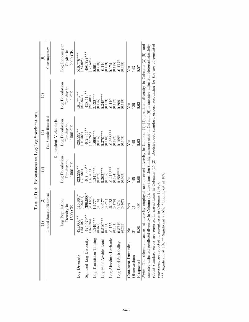
TableD.4:RobustnesstoLog-LogSpeci�cations
(1)
(2)
(3)
(4)
(5)
(6)
LimitedSampleHistorical
FullSampleHistorical
Contemporary
DependentVariableis:
LogPopulation
LogPopulation
LogPopulation
LogPopulation
LogIncomeper
Densityin
Densityin
Densityin
Densityin
Capitain
1500CE
1500CE
1000CE
1CE
2000CE
LogDiversity
451.066**
415.864*
423.298**
420.595**
481.771**
516.776***
(151.797)
(190.651)
(170.963)
(199.565)
(239.630)
(187.998)
SquaredLogDiversity
-425.579**
-396.906*
-407.990**
-402.344**
-458.413**
-480.727***
(150.883)
(204.655)
(159.515)
(185.258)
(222.306)
(176.526)
LogTransitionTiming
1.249***
1.177*
1.241***
1.606***
2.132***
0.061
(0.370)
(0.618)
(0.232)
(0.265)
(0.425)
(0.258)
Log%ofArableLand
0.510***
0.417*
0.392***
0.370***
0.348***
-0.119
(0.164)
(0.221)
(0.105)
(0.116)
(0.133)
(0.103)
LogAbsoluteLatitude
-0.155
-0.123
-0.413***
-0.368***
-0.110
0.174
(0.131)
(0.170)
(0.124)
(0.127)
(0.137)
(0.125)
LogLandSuitability
0.571*
0.674
0.256***
0.189*
0.209
-0.177*
(0.296)
(0.407)
(0.099)
(0.108)
(0.129)
(0.098)
ContinentDummies
No
Yes
Yes
Yes
Yes
Yes
Observations
2121
145
140
126
143
R-squared
0.89
0.91
0.69
0.62
0.62
0.57
Notes:TherelevantmeasuresofdiversityemployedareobserveddiversityinColumns(1)-(2),predicteddiversityinColumns(3)-(5),and
ancestry-adjustedpredicteddiversityinColumn(6).ThetransitiontimingmeasureusedinColumn(6)isancestryadjusted.Heteroskedasticity
robuststandarderrorsarereportedinparenthesesinColumns(1)-(2).Bootstrappedstandarderrors,accounting
fortheuseofgenerated
regressors,arereportedinparenthesesinColumns(3)-(6).
***Signi�cantat1%,**Signi�cantat5%,*Signi�cantat10%.
xxii

Table D.5: Robustness to Genetic Diversity Predicted by the Mobility Index
(1) (2) (3) (4)Full Sample Historical Contemporary
Dependent Variable is:
Log Population Log Population Log Population Log Income perDensity in Density in Density in Capita in1500 CE 1000 CE 1 CE 2000 CE
Diversity 152.163*** 146.551** 196.145** 176.090***(54.100) (64.082) (80.093) (67.405)
Diversity Squared -113.298*** -110.752** -148.569*** -120.996**(37.707) (44.392) (55.513) (47.536)
Log Transition Timing 1.553*** 2.052*** 3.242*** 0.047(0.255) (0.265) (0.349) (0.269)
Log % of Arable Land 0.362*** 0.314** 0.182 -0.144(0.111) (0.128) (0.126) (0.110)
Log Absolute Latitude -0.489*** -0.401*** -0.087 0.195(0.135) (0.146) (0.129) (0.142)
Log Land Suitability 0.256** 0.221* 0.301*** -0.148(0.101) (0.118) (0.116) (0.106)
Continent Dummies Yes Yes Yes YesObservations 127 123 113 125R-squared 0.71 0.66 0.69 0.55Notes : The relevant measures of diversity employed are genetic diversity predicted by the human-mobility indexin Columns (1)-(3), and its ancestry-adjusted counterpart in Column (4). The transition timing measure usedin Column (4) is ancestry adjusted as well. Bootstrapped standard errors, accounting for the use of generatedregressors, are reported in parentheses.*** Signi�cant at 1%, ** Signi�cant at 5%, * Signi�cant at 10%.
xxiii

TableD.6:Zeroth-andFirst-StageResultsof2SLSRegressions
(1)
(2)
(3)
(4)
(5)
(6)
Column5,Table2
Column6,Table2
0th-Stage
1st-Stage
0th-Stage
1st-Stage
DependentVariableis:
DependentVariableis:
Observed
Observed
Observed
Observed
Diversity
Observed
Observed
Diversity
Diversity
Diversity
Squared
Diversity
Diversity
Squared
2nd-StageExcludedInstr.:
MigratoryDistance
-0.814***
-5.143***
-5.841***
-0.657***
-3.992***
-4.234***
(0.064)
(0.686)
(0.959)
(0.196)
(0.850)
(1.053)
PredictedDiversitySqr.
�-3.937***
-4.327***
�-3.699***
-3.752***
(from0th-Stage)
(0.628)
(0.880)
(0.916)
(1.145)
2nd-StageControls:
LogTransitionTiming
-0.017**
-0.119***
-0.139***
-0.013**
-0.082***
-0.088***
(0.006)
(0.016)
(0.023)
(0.004)
(0.017)
(0.021)
Log%ofArableLand
0.000
0.004**
0.007**
0.002
0.015***
0.017***
(0.003)
(0.002)
(0.003)
(0.004)
(0.003)
(0.005)
LogAbsoluteLatitude
0.003*
0.018***
0.020***
0.005*
0.027***
0.028***
(0.002)
(0.002)
(0.003)
(0.002)
(0.006)
(0.007)
LogLandSuitability
0.005
0.032***
0.035***
0.005
0.031***
0.032***
(0.005)
(0.004)
(0.006)
(0.005)
(0.007)
(0.009)
ContinentDummies
No
No
No
Yes
Yes
Yes
Observations
2121
2121
2121
R-squared
0.96
0.99
0.99
0.98
0.99
0.99
Note:Heteroskedasticityrobuststandarderrorsarereportedinparentheses.
***Signi�cantat1%,**Signi�cantat5%,*Signi�cantat10%.
xxiv

TableD.7:RobustnesstotheEcologicalComponentsofLandProductivity
(1)
(2)
(3)
(4)
(5)
(6)
LimitedSampleHistorical
FullSampleHistorical
Contemporary
DependentVariableis:
LogPopulation
LogPopulation
LogPopulation
LogPopulation
LogIncomeper
Densityin
Densityin
Densityin
Densityin
Capitain
1500CE
1500CE
1000CE
1CE
2000CE
Diversity
236.192**
242.583**
171.881**
181.681**
195.610**
276.208***
(97.554)
(92.470)
(77.885)
(88.465)
(98.917)
(97.567)
DiversitySquared
-166.679**
-171.668**
-122.687**
-129.288**
-137.814**
-195.003***
(73.114)
(74.712)
(55.168)
(62.044)
(69.331)
(69.311)
LogTransitionTiming
1.565***
1.689*
1.214***
1.526***
1.839***
-0.027
(0.378)
(0.866)
(0.225)
(0.244)
(0.357)
(0.284)
Log%ofArableLand
0.547**
0.539
0.382***
0.338***
0.199*
-0.134
(0.192)
(0.313)
(0.091)
(0.093)
(0.104)
(0.089)
LogAbsoluteLatitude
0.183
0.221
-0.137
-0.124
0.292*
0.069
(0.160)
(0.289)
(0.166)
(0.170)
(0.150)
(0.164)
LogTemperature
1.520**
1.423
1.508***
1.971***
3.092***
-0.274
(0.591)
(0.993)
(0.535)
(0.558)
(0.580)
(0.458)
LogPrecipitation
0.714***
0.767*
0.358**
0.197
0.176
-0.236
(0.224)
(0.372)
(0.153)
(0.163)
(0.182)
(0.155)
LogSoilFertility
0.162
0.171
0.473
0.541
0.772**
-0.258
(0.554)
(0.579)
(0.303)
(0.329)
(0.359)
(0.297)
ContinentDummies
No
Yes
Yes
Yes
Yes
Yes
Observations
2121
145
140
126
143
R-squared
0.93
0.93
0.72
0.67
0.72
0.57
Notes:TherelevantmeasuresofdiversityemployedareobserveddiversityinColumns(1)-(2),predicteddiversityinColumns(3)-(5),and
ancestry-adjustedpredicteddiversityinColumn(6).ThetransitiontimingmeasureusedinColumn(6)isancestryadjusted.Themeasures
fortemperatureandprecipitationrepresenttheirrespectiveintertemporalaveragesduringthetimeperiod1961�1990andarecomputedusing
thegriddeddatasetofNew
etal.(2002).ThemeasureforsoilfertilityincoporatessoilcarbondensityandsoilpH,andisobtainedfrom
the
griddeddatasetofRamankuttyetal.(2002).Allthreemeasuresareaggregatedtothecountrylevelbyaveragingacrossthegridcellswithin
acountry.HeteroskedasticityrobuststandarderrorsarereportedinparenthesesinColumns(1)-(2).Bootstrappedstandarderrors,accounting
fortheuseofgeneratedregressors,arereportedinparenthesesinColumns(3)-(6).
***Signi�cantat1%,**Signi�cantat5%,*Signi�cantat10%.
xxv

TableD.8:RobustnesstotheSubsistenceModePrevalentin1000CE
(1)
(2)
(3)
(4)
(5)
(6)
LimitedSample1500CE
FullSample1500CE
FullSample1000CE
Baseline
w/Sub.Mode
Baseline
w/Sub.Mode
Baseline
w/Sub.Mode
DependentVariableis:
LogPopulation
LogPopulation
LogPopulation
Densityin
Densityin
Densityin
1500CE
1500CE
1000CE
Diversity
186.515**
180.340***
194.141**
196.984***
200.006**
241.019***
(67.317)
(51.275)
(76.265)
(56.215)
(96.042)
(60.902)
DiversitySquared
-131.922**
-129.882***
-142.349***
-144.055***
-145.722**
-173.861***
(51.717)
(39.681)
(53.585)
(40.161)
(66.585)
(42.845)
LogTransitionTiming
1.401
0.867
1.107***
1.013***
1.549***
1.388***
(0.826)
(0.849)
(0.254)
(0.210)
(0.320)
(0.252)
LogSubsistenceMode
1.678***
2.030***
2.543**
(0.465)
(0.730)
(0.996)
Log%ofArableLand
0.504**
0.453**
0.421***
0.458***
0.384***
0.447***
(0.191)
(0.150)
(0.101)
(0.097)
(0.123)
(0.114)
LogAbsoluteLatitude
-0.172
-0.158
-0.420***
-0.332***
-0.369***
-0.288**
(0.150)
(0.155)
(0.128)
(0.115)
(0.141)
(0.121)
LogLandSuitability
0.706**
0.413
0.226**
0.162*
0.173
0.067
(0.298)
(0.269)
(0.098)
(0.094)
(0.111)
(0.100)
ContinentDummies
Yes
Yes
Yes
Yes
Yes
Yes
Observations
2020
140
140
135
135
R-squared
0.90
0.92
0.67
0.72
0.58
0.67
Notes:Therelevantmeasuresofgeneticdiversityemployed
areobserved
diversityinColumns(1)-(2),andpredicteddiversityin
Columns(3)-(6).SubsistencemodeisacategoricalmeasurereportedatthelevelofaculturalgroupbyPeregrine(2003).Speci�cally,
themeasureassumesavalueof0intheabsenceofsedentaryagriculture,avalueof1/2whenagricultureispracticedbutonlyasa
secondarymodeofsubsistence,andavalueof1whenagricultureispracticedastheprimarymodeofsubsistence.Themeasureis
aggregatedtothecountrylevelbyaveragingacrosstheculturalgroupsthat,intheyear1000CE,residedinregionswithinthemodern
nationalbordersofacountry.HeteroskedasticityrobuststandarderrorsarereportedinparenthesesinColumns(1)-(2).Bootstrapped
standarderrors,accountingfortheuseofgeneratedregressors,arereportedinparenthesesinColumns(3)-(6).
***Signi�cantat1%,**Signi�cantat5%,*Signi�cantat10%.
xxvi

Table D.9: Adjusted Migratory Distance vs. Alternative Distances
(1) (2) (3) (4)
Dependent Variable isLog Income Per Capita in 2000 CE
Migratory Distance 0.601*** 0.499*** 0.532*** 0.564**(Ancestry Adjusted) (0.073) (0.124) (0.160) (0.235)
Migratory Distance Sqr. -0.030*** -0.026*** -0.027*** -0.029***(Ancestry Adjusted) (0.004) (0.006) (0.008) (0.010)
Migratory Distance 0.078(Unadjusted) (0.084)
Migratory Distance Sqr. -0.002(Unadjusted) (0.003)
Aerial Distance 0.064(Unadjusted) (0.201)
Aerial Distance Sqr. -0.002(Unadjusted) (0.011)
Aerial Distance 0.043(Ancestry Adjusted) (0.330)
Aerial Distance Sqr. -0.001(Ancestry Adjusted) (0.018)
Observations 109 109 109 109R-squared 0.28 0.29 0.29 0.29Note : Heteroskedasticity robust standard errors are reported in parentheses.*** Signi�cant at 1%, ** Signi�cant at 5%, * Signi�cant at 10%.
xxvii

TableD.10:RobustnesstoFstGeneticDistances
(1)
(2)
(3)
(4)
(5)
(6)
LimitedSampleHistorical
FullSampleHistorical
Contemporary
Baseline
w/Gen.Dist.
Baseline
w/Gen.Dist.
Baseline
w/Gen.Dist.
DependentVariableis:
LogPopulation
LogPopulation
LogIncomeper
Densityin
Densityin
Capitain
1500CE
1500CE
2000CE
Diversity
184.672**
201.230**
194.681**
194.743**
185.512**
212.380**
(63.338)
(65.970)
(81.638)
(85.603)
(86.160)
(99.759)
DiversitySquared
-130.466**
-144.435**
-142.204**
-145.347**
-128.045**
-150.435**
(48.774)
(50.450)
(57.192)
(60.802)
(61.150)
(71.184)
LogTransitionTiming
1.150*
1.044
1.236***
1.025***
-0.218
-0.122
(0.634)
(0.915)
(0.242)
(0.312)
(0.285)
(0.347)
Log%ofArableLand
0.433**
0.314
0.392***
0.362***
-0.155
-0.136
(0.172)
(0.396)
(0.099)
(0.107)
(0.100)
(0.102)
LogAbsoluteLatitude
-0.138
-0.160
-0.419***
-0.477***
0.068
0.077
(0.150)
(0.184)
(0.122)
(0.128)
(0.117)
(0.124)
LogLandSuitability
0.636*
0.778
0.259***
0.324***
-0.147
-0.148
(0.294)
(0.559)
(0.095)
(0.097)
(0.093)
(0.092)
GeneticDistancetotheU.K.
-0.014
-0.027
(1500match)
(0.049)
(0.027)
GeneticDistancetoEthiopia
-0.047
-0.069
(1500match)
(0.084)
(0.043)
GeneticDistancetotheU.S.
0.030
(weighted)
(0.037)
GeneticDistancetoEthiopia
-0.075*
(weighted)
(0.043)
ContinentDummies
Yes
Yes
Yes
Yes
Yes
Yes
Observations
2020
142
142
139
139
R-squared
0.91
0.91
0.69
0.71
0.61
0.62
Notes:TherelevantmeasuresofdiversityemployedareobserveddiversityinColumns(1)-(2),predicteddiversityinColumns(3)-(4),and
ancestry-adjustedpredicteddiversityinColumns(5)-(6).ThetransitiontimingmeasureusedinColumns(5)-(6)isancestryadjustedas
well.HeteroskedasticityrobuststandarderrorsarereportedinparenthesesinColumns(1)-(2).Bootstrappedstandarderrors,accounting
fortheuseofgeneratedregressors,arereportedinparenthesesinColumns(3)-(6).
***Signi�cantat1%,**Signi�cantat5%,*Signi�cantat10%.
xxviii

Table D.11: Robustness to Regional Fixed E¤ects and Sub-Sampling on Regional Clusters
(1) (2) (3) (4) (5)Full w/out w/out w/out SSA only SSA
Sample SSA LAC & LAC & LAC
Dependent Variable is Log Income Per Capita in 2000 CE
Predicted Diversity 299.370*** 285.108*** 492.169*** 597.082*** 250.578***(Ancestry Adjusted) (63.294) (89.612) (141.359) (194.662) (86.422)
Predicted Diversity Sqr. -209.044*** -199.109*** -342.630*** -415.660*** -175.074***(Ancestry Adjusted) (45.538) (65.355) (98.352) (137.757) (62.321)
Log Transition Timing 0.293* 0.023 0.352* -0.033 0.359(Ancestry Adjusted) (0.173) (0.236) (0.208) (0.269) (0.271)
Log % of Arable Land -0.188*** -0.195*** -0.192*** -0.152** -0.173**(0.048) (0.071) (0.043) (0.067) (0.070)
Log Absolute Latitude -0.044 0.131 -0.189 -0.173 -0.037(0.090) (0.120) (0.114) (0.153) (0.111)
Social Infrastructure 1.156** 0.790* 1.525** 0.868 0.413(0.465) (0.433) (0.601) (0.609) (0.920)
Ethnic Fractionalization -0.338 0.147 -0.739** -0.511* -0.282(0.257) (0.283) (0.284) (0.296) (0.450)
% of Population at Risk of -0.671** -0.561** -0.426 0.121 -1.135**Contracting Malaria (0.301) (0.267) (0.416) (0.320) (0.425)
% of Population Living in -0.307 -0.557*** -0.469** -0.976*** -0.129Tropical Zones (0.190) (0.192) (0.219) (0.265) (0.223)
Mean Distance to Nearest -0.384** -0.797*** -0.416*** -0.665** -0.275Waterway (0.180) (0.246) (0.149) (0.247) (0.240)
Optimal Diversity 0.716*** 0.716*** 0.718*** 0.718*** 0.716***(0.008) (0.011) (0.006) (0.007) (0.013)
Observations 109 71 87 49 60R-squared 0.90 0.89 0.93 0.94 0.80Notes : Bootstrapped standard errors, accounting for the use of generated regressors, are reported inparentheses. All regressions include controls for an OPEC dummy, legal origin dummies, and major religionshares, as well as regional dummies for (i) Sub-Saharan Africa (except Columns (2) and (4)), (ii) MiddleEast and North Africa, (iii) Europe and Central Asia, (iv) South Asia, (v) East Asia and Paci�c, and (vi)Latin America and Caribbean (except Columns (3)-(5)).*** Signi�cant at 1%, ** Signi�cant at 5%, * Signi�cant at 10%.
xxix

TableD.12:RobustnesstoPercentageofthePopulationofEuropeanDescent
(1)
(2)
(3)
(4)
(5)
(6)
(7)
(8)
Full
Full
Non
Non
w/oNeo
w/oNeo
Non
Non
Sample
Sample
OECD
OECD
Europes
Europes
European
European
DependentVariableisLogIncomePerCapitain2000CE
PredictedDiversity
277.342***
272.274***
271.979***
263.805**
261.367***
272.904***
280.902***
280.957**
(AncestryAdjusted)
(69.452)
(83.202)
(84.232)
(115.923)
(69.946)
(89.295)
(76.868)
(111.552)
PredictedDiversitySqr.
-192.386***
-188.868***
-188.974***
-183.258**
-181.811***
-189.886***
-195.093***
-195.132**
(AncestryAdjusted)
(49.056)
(58.239)
(59.200)
(80.816)
(49.261)
(62.495)
(54.133)
(77.587)
LogTransitionTiming
0.396*
0.383
0.390
0.373
0.355
0.386
0.480*
0.480
(AncestryAdjusted)
(0.233)
(0.242)
(0.281)
(0.302)
(0.231)
(0.249)
(0.278)
(0.299)
Log%ofArableLand
-0.183***
-0.183***
-0.236***
-0.235***
-0.201***
-0.202***
-0.198***
-0.198***
(0.051)
(0.051)
(0.060)
(0.060)
(0.055)
(0.055)
(0.055)
(0.055)
LogAbsoluteLatitude
0.009
0.007
-0.021
-0.022
-0.025
-0.024
0.016
0.016
(0.108)
(0.108)
(0.119)
(0.122)
(0.111)
(0.112)
(0.112)
(0.115)
SocialInfrastructure
1.826***
1.810***
1.313**
1.304**
1.416***
1.426***
1.790***
1.790***
(0.417)
(0.436)
(0.579)
(0.615)
(0.507)
(0.517)
(0.464)
(0.547)
EthnicFractionalization
-0.333
-0.336
-0.437
-0.446
-0.390
-0.386
-0.384
-0.384
(0.280)
(0.291)
(0.375)
(0.402)
(0.300)
(0.302)
(0.359)
(0.374)
%ofPopulationatRiskof
-0.502
-0.495
-0.605
-0.591
-0.591
-0.612
-0.511
-0.511
ContractingMalaria
(0.351)
(0.380)
(0.381)
(0.443)
(0.370)
(0.408)
(0.380)
(0.433)
%ofPopulationLivingin
-0.319
-0.312
-0.196
-0.184
-0.302
-0.318
-0.276
-0.276
TropicalZones
(0.204)
(0.212)
(0.239)
(0.257)
(0.219)
(0.228)
(0.232)
(0.254)
MeanDistancetoNearest
-0.368**
-0.367*
-0.387*
-0.382*
-0.452**
-0.461**
-0.315
-0.315
Waterway
(0.186)
(0.190)
(0.222)
(0.229)
(0.210)
(0.215)
(0.206)
(0.208)
%ofPopulationofEuropean
0.061
0.095
-0.157
-0.001
Descent
(0.621)
(0.902)
(0.700)
(0.891)
OptimalDiversity
0.721***
0.721***
0.720***
0.720***
0.719***
0.719***
0.720***
0.720***
(0.068)
(0.089)
(0.085)
(0.195)
(0.015)
(0.022)
(0.021)
(0.036)
Observations
109
109
8383
105
105
8888
R-squared
0.90
0.90
0.82
0.82
0.89
0.89
0.84
0.84
Notes:Bootstrappedstandarderrors,accountingfortheuseofgeneratedregressors,arereportedinparentheses.Allregressionsincludecontrolsformajor
religionsharesaswellasOPEC,legalorigin,sub-SaharanAfricaandcontinentdummies.
***Signi�cantat1%,**Signi�cantat5%,*Signi�cantat10%.
xxx

TableD.13:StandardizedBetasandPartialR-squaresintheBaselineRegressions
(1)
(2)
(3)
(4)
(5)
(6)
LimitedSampleHistorical
FullSampleHistorical
Contemporary
Tbl.1,Col.4
Tbl.1,Col.5
Tbl.3,Col.6
Tbl.A.1,Col.6
Tbl.A.2,Col.6
Tbl.6,Col.2
DependentVariableis:
LogPopulation
LogPopulation
LogPopulation
LogPopulation
LogIncome
Densityin
Densityin
Densityin
Densityin
perCapitain
1500CE
1500CE
1000CE
1CE
2000CE
Diversity
7.203
6.512
7.008
6.955
7.540
5.510
[0.32]
[0.21]
[0.07]
[0.06]
[0.06]
[0.03]
DiversitySquared
-6.913
-6.251
-6.936
-6.838
-7.364
-5.485
[0.30]
[0.18]
[0.07]
[0.06]
[0.06]
[0.03]
LogTransitionTiming
0.372
0.348
0.490
0.653
0.765
0.024
[0.35]
[0.24]
[0.20]
[0.28]
[0.34]
[0.00]
Log%ofArableLand
0.343
0.363
0.315
0.304
0.256
-0.120
[0.29]
[0.24]
[0.11]
[0.08]
[0.06]
[0.01]
LogAbsoluteLatitude
-0.109
-0.086
-0.257
-0.236
-0.069
0.136
[0.06]
[0.03]
[0.10]
[0.07]
[0.01]
[0.02]
LogLandSuitability
0.291
0.299
0.225
0.173
0.163
-0.201
[0.32]
[0.32]
[0.06]
[0.03]
[0.03]
[0.03]
ContinentDummies
No
Yes
Yes
Yes
Yes
Yes
Observations
2121
145
140
126
143
R-squared
0.89
0.90
0.69
0.62
0.61
0.57
Notes:TherelevantmeasuresofdiversityemployedareobserveddiversityinColumns(1)-(2),predicteddiversityinColumns(3)-(5),andancestry-
adjustedpredicteddiversityinColumn(6).ThetransitiontimingmeasureusedinColumn(6)isancestryadjusted.PartialR-squaresarereported
insquarebrackets.Thestandardizedbetasarereportedinunitsofastandarddeviationinthedependentvariable.
xxxi

Table D.14: Trust, Scienti�c Productivity, and Economic Development in 2000 CE
(1) (2) (3) (4) (5) (6)
Dependent Variable is Log Income Per Capita in 2000 CE
Interpersonal Trust 3.715*** 2.359*** 1.724***(0.702) (0.660) (0.591)
Scienti�c Articles 3.391*** 1.969*** 1.429***(0.312) (0.334) (0.292)
Log Transition Timing -0.239 -0.330 -0.113 -0.042(Ancestry Adjusted) (0.290) (0.294) (0.268) (0.187)
Log % of Arable Land -0.223* -0.226* -0.090 -0.026(0.119) (0.117) (0.098) (0.074)
Log Absolute Latitude 0.351** -0.201 0.166 0.014(0.135) (0.248) (0.105) (0.108)
Log Land Suitability 0.177 0.122 -0.101 -0.141*(0.110) (0.090) (0.112) (0.081)
Executive Constraints 0.163*** 0.109**(0.051) (0.044)
Ethnic Fractionalization -0.721** -0.667**(0.348) (0.332)
% of Population at Risk of -1.115*** -1.285***Contracting Malaria (0.407) (0.267)
% of Population Living in -0.559 0.086Tropical Zones (0.551) (0.253)
Mean Distance to Nearest 0.063 -0.176Waterway (0.096) (0.159)
Observations 73 73 73 125 125 125R-squared 0.27 0.68 0.84 0.41 0.68 0.80Notes : Heteroskedasticity robust standard errors are reported in parentheses. Columns (2)-(3) and (5)-(6)also include controls for sub-Saharan Africa and continent dummies. Columns (3) and (6) additionallyinclude controls for OPEC and legal origin dummies.*** Signi�cant at 1%, ** Signi�cant at 5%, * Signi�cant at 10%.
xxxii

E The HGDP-CEPH Sample of 53 Ethnic Groups
Ethnic Group Migratory Distance Country Region(in km)
Bantu (Kenya) 1,338.94 Kenya AfricaBantu (Southeast) 4,306.19 South Africa AfricaBantu (Southwest) 3,946.44 Namibia AfricaBiaka Pygmy 2,384.86 Central African Republic AfricaMandenka 5,469.91 Senegal AfricaMbuti Pygmy 1,335.50 Zaire AfricaSan 3,872.42 Namibia AfricaYoruba 3,629.65 Nigeria Africa
Bedouin 2,844.95 Israel Middle EastDruze 2,887.25 Israel Middle EastMozabite 4,418.17 Algeria Middle EastPalestinian 2,887.25 Israel Middle East
Adygei 4,155.03 Russia EuropeBasque 6,012.26 France EuropeFrench 5,857.48 France EuropeItalian 5,249.04 Italy EuropeOrcadian 6,636.69 United Kingdom EuropeRussian 5,956.40 Russia EuropeSardinian 5,305.81 Italy EuropeTuscan 5,118.37 Italy Europe
Balochi 5,842.06 Pakistan AsiaBrahui 5,842.06 Pakistan AsiaBurusho 6,475.60 Pakistan AsiaCambodian 10,260.55 Cambodia AsiaDai 9,343.96 China AsiaDaur 10,213.13 China AsiaHan 10,123.19 China AsiaHan (North China) 9,854.75 China AsiaHazara 6,132.57 Pakistan AsiaHezhen 10,896.21 China AsiaJapanese 11,762.11 Japan AsiaKalash 6,253.62 Pakistan AsiaLahu 9,299.63 China AsiaMakrani 5,705.00 Pakistan AsiaMiao 9,875.32 China AsiaMongola 9,869.85 China AsiaNaxi 9,131.37 China AsiaOroqen 10,290.53 China AsiaPathan 6,178.76 Pakistan AsiaShe 10,817.81 China AsiaSindhi 6,201.70 Pakistan AsiaTu 8,868.14 China AsiaTujia 9,832.50 China AsiaUygur 7,071.97 China AsiaXibo 7,110.29 China AsiaYakut 9,919.11 Russia (Siberia) AsiaYi 9,328.79 China Asia
Melanesian 16,168.51 Papua New Guinea OceaniaPapuan 14,843.12 Papua New Guinea Oceania
Colombian 22,662.78 Colombia AmericasKaritiana 24,177.34 Brazil AmericasMaya 19,825.71 Mexico AmericasPima 18,015.79 Mexico Americas
xxxiii

F Variable De�nitions and Sources
Outcome Variables:
Population Density in 1 CE, 1000 CE, and 1500 CE. Population density (in persons per square km)for given year is calculated as population in that year, as reported by McEvedy and Jones (1978), dividedby total land area, as reported by the World Bank�s World Development Indicators. The cross-sectional unitof observation in McEvedy and Jones�s (1978) data set is a region delineated by its international borders in1975. Historical population estimates are provided for regions corresponding to either individual countriesor, in some cases, to sets comprised of 2�3 neighboring countries (e.g., India, Pakistan and Bangladesh). Inthe latter case, a set-speci�c population density �gure is calculated based on total land area and the �gureis then assigned to each of the component countries in the set. The same methodology is also employed toobtain population density for countries that exist today but were part of a larger political unit (e.g., the formerYugoslavia) in 1975. The data reported by the authors are based on a wide variety of country and region-speci�c historical sources, the enumeration of which would be impractical for this appendix. The interestedreader is therefore referred to McEvedy and Jones (1978) for more details on the original data sources citedtherein.
Income Per Capita in 2000 CE. Real GDP per capita, in constant 2000 international dollars, as reportedby the Penn World Table, version 6.2.
Interpersonal Trust. The fraction of total respondents within a given country, from �ve di¤erent waves of theWorld Values Survey conducted during the time period 1981�2008, that responded with "Most people can betrusted" (as opposed to "Can�t be too careful") when answering the survey question "Generally speaking,wouldyou say that most people can be trusted or that you can�t be too careful in dealing with people?"
Scienti�c Articles. The mean, over the period 1981-2000, of the annual number of scienti�c articles percapita, calculated as the total number of scienti�c and technical articles published in a given year divided bythe total population in that year. The relevant data on the total number of articles and population in a givenyear are obtained from the World Bank�s World Development Indicators.
Genetic Diversity Variables:
Observed Genetic Diversity in the Limited Historical Sample. The average expected heterozygosityacross ethnic groups from the Human Genome Diversity Cell Line Panel that are located within a givencountry. The expected heterozygosities of the ethnic groups are from Ramachandran et al. (2005).
Predicted Genetic Diversity in the Extended Historical Sample. The expected heterozygosity (geneticdiversity) of a given country as predicted by (the extended sample de�nition of) migratory distance fromAddis Ababa (Ethiopia). This measure is calculated by applying the regression coe¢ cients obtained fromregressing expected heterozygosity on migratory distance at the ethnic group level, using the worldwide sampleof 53 ethnic groups from the Human Genome Diversity Cell Line Panel. The expected heterozygosities andgeographical coordinates of the ethnic groups are from Ramachandran et al. (2005).
Note that for Table D.5 in Appendix D, the migratory distance concept used to predict the genetic diversityof a country�s population is the human-mobility index, calculated for the journey from Addis Ababa (Ethiopia)to the country�s modern capital city, as opposed to the default waypoints-restricted migratory distance conceptused elsewhere. For additional details on how the human-mobility index is calculated, the interested reader isreferred to the de�nition of this variable further below.
Predicted Genetic Diversity (Ancestry Adjusted). The expected heterozygosity (genetic diversity) ofa country�s population, predicted by migratory distances from Addis Ababa (Ethiopia) to the year 1500 CElocations of the ancestral populations of the country�s component ethnic groups in 2000 CE, as well as by
xxxiv
pairwise migratory distances between these ancestral populations. The source countries of the year 1500 CEancestral populations are identi�ed from theWorld Migration Matrix, 1500�2000, discussed in Putterman andWeil (2010), and the modern capital cities of these countries are used to compute the aforementioned migratorydistances. The measure of genetic diversity is then calculated by applying (i) the regression coe¢ cients obtainedfrom regressing expected heterozygosity on migratory distance from Addis Ababa at the ethnic group level,using the worldwide sample of 53 ethnic groups from the Human Genome Diversity Cell Line Panel, (ii) theregression coe¢ cients obtained from regressing pairwise Fst genetic distances on pairwise migratory distancesbetween these ethnic groups, and (iii) the ancestry weights representing the fractions of the year 2000 CEpopulation (of the country for which the measure is being computed) that can trace their ancestral originsto di¤erent source countries in the year 1500 CE. The construction of this measure is discussed in detail inAppendix B. The expected heterozygosities, geographical coordinates, and pairwise Fst genetic distances ofthe 53 ethnic groups are from Ramachandran et al. (2005). The ancestry weights are from theWorld MigrationMatrix, 1500�2000.
Note that, in contrast to the default waypoints-restricted migratory distance concept used elsewhere, themigratory distance concept used to predict the ancestry-adjusted genetic diversity of a country�s population forTable D.5 in Appendix D is the human-mobility index, calculated for the journey from Addis Ababa (Ethiopia)to each of the year 1500 CE locations of the ancestral populations of the country�s component ethnic groups in2000 CE, as well as for the journey between each pair of these ancestral populations. For additional details onhow the human-mobility index is calculated, the interested reader is referred to the de�nition of this variablefurther below.
Distance Variables:
Migratory Distance from Addis Ababa in the Limited Historical Sample. The average migratorydistance across ethnic groups from the Human Genome Diversity Cell Line Panel that are located within a givencountry. The migratory distance of an ethnic group is the great circle distance from Addis Ababa (Ethiopia)to the location of the group, along a land-restricted path forced through one or more of �ve intercontinentalwaypoints, including Cairo (Egypt), Istanbul (Turkey), Phnom Penh (Cambodia), Anadyr (Russia) and PrinceRupert (Canada). Distances are calculated using the Haversine formula and are measured in units of 1,000 km.The geographical coordinates of the ethnic groups and the intercontinental waypoints are from Ramachandranet al. (2005).
Migratory Distance from Addis Ababa in the Extended Historical Sample. The great circle distancefrom Addis Ababa (Ethiopia) to the country�s modern capital city, along a land-restricted path forced throughone or more of �ve aforementioned intercontinental waypoints. Distances are calculated using the Haversineformula and are measured in units of 1,000 km. The geographical coordinates of the intercontinental waypointsare from Ramachandran et al. (2005), while those of the modern capital cities are from the CIA�s WorldFactbook.
Migratory Distance from Addis Ababa (Ancestry Adjusted). The cross-country weighted averageof (the extended sample de�nition of) migratory distance from Addis Ababa (Ethiopia), where the weightassociated with a given country in the calculation represents the fraction of the year 2000 CE population (ofthe country for which the measure is being computed) that can trace its ancestral origins to the given countryin the year 1500 CE. The ancestry weights are obtained from the World Migration Matrix, 1500�2000 ofPutterman and Weil (2010).
Migratory Distance from a �Placebo� Point of Origin. The great circle distance from a �placebo�location (i.e., other than Addis Ababa, Ethiopia) to the country�s modern capital city, along a land-restrictedpath forced through one or more of �ve aforementioned intercontinental waypoints. Distances are calculatedusing the Haversine formula and are measured in units of 1,000 km. The geographical coordinates of theintercontinental waypoints are from Ramachandran et al. (2005), while those of the modern capital cities are
xxxv

from the CIA�s World Factbook. The �placebo� locations for which results are presented in the text includeLondon (UK), Tokyo (Japan), and Mexico City (Mexico).
Aerial Distance from Addis Ababa. The great circle distance �as the crow �ies� from Addis Ababa(Ethiopia) to the country�s modern capital city. Distances are calculated using the Haversine formula andare measured in units of 1,000 km. The geographical coordinates of capital cities are from the CIA�s WorldFactbook.
Aerial Distance from Addis Ababa (Ancestry Adjusted). The cross-country weighted average of aerialdistance from Addis Ababa, where the weight associated with a given country in the calculation representsthe fraction of the year 2000 CE population (of the country for which the measure is being computed) thatcan trace its ancestral origins to the given country in the year 1500 CE. The ancestry weights are from theWorld Migration Matrix, 1500�2000 of Putterman and Weil (2010).
Distance to Frontier in 1 CE, 1000 CE, and 1500 CE. The great circle distance from a country�scapital city to the closest regional technological frontier for a given year. The year-speci�c set of regionalfrontiers comprises the two most populous cities, reported for that year and belonging to di¤erent civilizationsor sociopolitical entities, from each of Africa, Europe, Asia, and the Americas. Distances are calculated usingthe Haversine formula and are measured in km. The historical urban population data, used to identify thefrontiers, are obtained from Chandler (1987) and Modelski (2003), and the geographical coordinates of ancienturban centers are obtained using Wikipedia.
Human Mobility Index. The average migratory distance across ethnic groups from the Human GenomeDiversity Cell Line Panel that are located within a given country. The migratory distance of an ethnic groupis the distance from Addis Ababa (Ethiopia) to the location of the group, along an �optimal�land-restrictedpath that minimizes the time cost of travelling on the surface of the Earth in the absence of steam-poweredtransportation technologies. The optimality of a path is determined by incorporating information on naturalimpediments to human spatial mobility such as the meteorological and topographical conditions prevalentalong the path, as well as information on the time cost of travelling under such conditions as reported byHayes (1996). Distances are measured in weeks of travel time. The geographical coordinates of the ethnicgroups are from Ramachandran et al. (2005). The methodology underlying the construction of this index isdiscussed in greater detail by Ashraf et al. (2010) and Özak (2010).
Genetic Distance to the U.K./Ethiopia (1500 Match). The Fst genetic distance, as reported bySpolaore and Wacziarg (2009), between the year 1500 CE populations of a given country and the U.K. (orEthiopia), calculated as the genetic distance between the two ethnic groups comprising the largest shares ofeach country�s population in the year 1500 CE.
Genetic Distance to the U.S./Ethiopia (Weighted). The Fst genetic distance, as reported by Spolaoreand Wacziarg (2009), between the contemporary national populations of a given country and the U.S. (orEthiopia), calculated as the average pairwise genetic distance across all ethnic group pairs, where each paircomprises two distinct ethnic groups, one from each country, and is weighted by the product of the proportionalrepresentations of the two groups in their respective national populations.
Transition Timing and Subsistence Mode Variables:
Neolithic Transition Timing. The number of thousand years elapsed, until the year 2000, since the majorityof the population residing within a country�s modern national borders began practicing sedentary agricultureas the primary mode of subsistence. This measure, reported by Putterman (2008), is compiled using a widevariety of both regional and country-speci�c archaeological studies as well as more general encyclopedic workson the transition from hunting and gathering to agriculture during the Neolithic. The reader is referred to
xxxvi

the author�s web site for a detailed description of the primary and secondary data sources employed by theauthor in the construction of this variable.
Neolithic Transition Timing (Ancestry Adjusted). The cross-country weighted average of Neolithictransition timing, where the weight associated with a given country in the calculation represents the fractionof the year 2000 CE population (of the country for which the measure is being computed) that can trace itsancestral origins to the given country in the year 1500 CE. The ancestry weights are obtained from the WorldMigration Matrix, 1500�2000 of Putterman and Weil (2010).
Subsistence Mode in 1000 CE. An index in the [0,1]-interval that gauges the extent to which sedentaryagriculture was practiced, in the year 1000 CE, within a region delineated by a country�s modern internationalborders. This index is constructed using data from Peregrine�s (2003) Atlas of Cultural Evolution, whichreports, amongst other variables, a measure of the mode of subsistence on a 3-point categorical scale at the levelof a cultural group (or �archaeological tradition�) that existed in the year 1000 CE. Speci�cally, the measureis taken to assume a value of 0 in the absence of sedentary agriculture (i.e., if the cultural group exclusivelypracticed hunting and gathering), a value of 12 when agriculture was practiced but only as a secondary modeof subsistence, and a value of 1 when agriculture was practiced as the primary mode of subsistence. Giventhat the cross-sectional unit of observation in Peregrine�s (2003) data set is a cultural group, speci�c to a givenregion on the global map, and since spatial delineations of groups, as reported by Peregrine (2003), do notnecessarily correspond to contemporary international borders, the measure is aggregated to the country levelby averaging across those cultural groups that are reported to appear within the modern borders of a givencountry. For more details on the underlying data employed to construct this index, the interested reader isreferred to Peregrine (2003).
Geographical Variables:
Percentage of Arable Land. The fraction of a country�s total land area that is arable, as reported by theWorld Bank�s World Development Indicators.
Absolute Latitude. The absolute value of the latitude of a country�s approximate geodesic centroid, asreported by the CIA�s World Factbook.
Land Suitability for Agriculture. A geospatial index of the suitability of land for agriculture based onecological indicators of climate suitability for cultivation, such as growing degree days and the ratio of actualto potential evapotranspiration, as well as ecological indicators of soil suitability for cultivation, such as soilcarbon density and soil pH. This index was initially reported at a half-degree resolution by Ramankutty et al.(2002). Formally, Ramankutty et al. (2002) calculate the land suitability index (S) as the product of climatesuitability (Sclim) and soil suitability (Ssoil), i.e., S = Sclim � Ssoil. The climate suitability component isestimated to be a function of growing degree days (GDD) and a moisture index (�) gauging water availabilityto plants, calculated as the ratio of actual to potential evapotranspiration, i.e., Sclim = f1(GDD)f2(�). Thesoil suitability component, on the other hand, is estimated to be a function of soil carbon density (Csoil) and soilpH (pHsoil), i.e. Ssoil = g1(Csoil)g2(pHsoil). The functions, f1(GDD), f2(�), g1(Csoil), and g2(pHsoil)are chosen by Ramankutty et al. (2002) by empirically �tting functions to the observed relationships betweencropland areas, GDD, �, Csoil, and pHsoil. For more details on the speci�c functional forms chosen, theinterested reader is referred to Ramankutty et al. (2002). Since Ramankutty et al. (2002) report theland suitability index at a half-degree resolution, Michalopoulos (2011) aggregates the index to the countrylevel by averaging land suitability across grid cells within a country. This study employs the country-levelaggregate measure reported by Michalopoulos (2011) as the control for land suitability in the baseline regressionspeci�cations for both historical population density and contemporary income per capita.
Range of Land Suitability. The di¤erence between the maximum and minimum values of a land suitabilityindex, reported at a half-degree resolution by Ramankutty et al. (2002), across grid cells within a country. This
xxxvii

variable is obtained from the data set of Michalopoulos (2011). For additional details on the land suitabilityindex, the interested reader is referred to the de�nition of the land suitability variable above.
Land Suitability Gini. The Gini coe¢ cient based on the distribution of a land suitability index, reportedat a half-degree resolution by Ramankutty et al. (2002), across grid cells within a country. This variable isobtained from the data set of Michalopoulos (2011). For additional details on the land suitability index, theinterested reader is referred to the de�nition of the land suitability variable above.
Soil Fertility. The soil suitability component of an index of land suitability for agriculture, based on soilcarbon density and soil pH. The soil suitability data are reported at a half-degree resolution by Ramankuttyet al. (2000) and are aggregated to the country level by Michalopoulos (2011) by averaging across grid cellswithin a country. For additional details on the soil suitability component of the land suitability index, theinterested reader is referred to the de�nition of the land suitability variable above.
Mean Elevation. The mean elevation of a country in km above sea level, calculated using geospatial elevationdata reported by the G-ECON project (Nordhaus, 2006) at a 1-degree resolution, which, in turn, is based onsimilar but more spatially disaggregated data at a 10-minute resolution from New et al. (2002). The measureis thus the average elevation across the grid cells within a country. The interested reader is referred to theG-ECON project web site for additional details.
Standard Deviation of Elevation. The standard deviation of elevation across the grid cells within acountry in km above sea level, calculated using geospatial elevation data reported by the G-ECON project(Nordhaus, 2006) at a 1-degree resolution, which, in turn, is based on similar but more spatially disaggregateddata at a 10-minute resolution from New et al. (2002). The interested reader is referred to the G-ECONproject web site for additional details.
Terrain Roughness. The degree of terrain roughness of a country, calculated using geospatial surfaceundulation data reported by the G-ECON project (Nordhaus, 2006) at a 1-degree resolution, which is basedon more spatially disaggregated elevation data at a 10-minute resolution from New et al. (2002). The measureis thus the average degree of terrain roughness across the grid cells within a country. The interested reader isreferred to the G-ECON project web site for additional details.
Temperature. The intertemporal average monthly temperature of a country in degrees Celsius per monthover the 1961�1990 time period, calculated using geospatial average monthly temperature data for this periodreported by the G-ECON project (Nordhaus, 2006) at a 1-degree resolution, which, in turn, is based on similarbut more spatially disaggregated data at a 10-minute resolution from New et al. (2002). The measure is thusthe spatial mean of the intertemporal average monthly temperature across the grid cells within a country. Theinterested reader is referred to the G-ECON project web site for additional details.
Precipitation. The intertemporal average monthly precipitation of a country in mm per month over the 1961�1990 time period, calculated using geospatial average monthly precipitation data for this period reported bythe G-ECON project (Nordhaus, 2006) at a 1-degree resolution, which, in turn, is based on similar but morespatially disaggregated data at a 10-minute resolution from New et al. (2002). The measure is thus the spatialmean of the intertemporal average monthly precipitation across the grid cells within a country. The interestedreader is referred to the G-ECON project web site for additional details.
Mean Distance to Nearest Waterway. The distance, in thousands of km, from a GIS grid cell to thenearest ice-free coastline or sea-navigable river, averaged across the grid cells of a country. This variable wasoriginally constructed by Gallup et al. (1999) and is part of Harvard University�s CID Research Datasets onGeneral Measures of Geography.
xxxviii

Percentage of Land within 100 km of Waterway. The percentage of a country�s total land area that islocated within 100 km of an ice-free coastline or sea-navigable river. This variable was originally constructedby Gallup et al. (1999) and is part of Harvard University�s CID Research Datasets on General Measures ofGeography.
Percentage of Population Living in Tropical Zones. The percentage of a country�s population in 1995that resided in areas classi�ed as tropical by the Köppen-Geiger climate classi�cation system. This variablewas originally constructed by Gallup et al. (1999) and is part of Harvard University�s CID Research Datasetson General Measures of Geography.
Percentage of Population at Risk of Contracting Malaria. The percentage of a country�s population in1994 residing in regions of high malaria risk, multiplied by the proportion of national cases involving the fatalspecies of the malaria pathogen, P. falciparum (as opposed to other largely non-fatal species). This variablewas originally constructed by Gallup and Sachs (2001) and is part of Columbia University�s Earth Institutedata set on malaria.
Climate. An index of climatic suitability for agriculture, based on the Köppen-Geiger climate classi�cationsystem. This variable is obtained from the data set of Olsson and Hibbs (2005).
Orientation of Continental Axis. The orientation of a continent (or landmass) along a North-South orEast-West axis. This measure, reported in the data set of Olsson and Hibbs (2005), is calculated as the ratio ofthe largest longitudinal (East-West) distance to the largest latitudinal (North-South) distance of the continent(or landmass).
Size of Continent. The total land area of a continent (or landmass) as reported in the data set of Olssonand Hibbs (2005).
Domesticable Plants. The number of annual and perennial wild grass species, with a mean kernel weightexceeding 10 mg, that were prehistorically native to the region to which a country belongs. This variable isobtained from the data set of Olsson and Hibbs (2005).
Domesticable Animals. The number of domesticable large mammalian species, weighing in excess of 45kg, that were prehistorically native to the region to which a country belongs. This variable is obtained fromthe data set of Olsson and Hibbs (2005).
Institutional, Cultural, and Human Capital Variables:
Social Infrastructure. An index, calculated by Hall and Jones (1999), that quanti�es the wedge betweenprivate and social returns to productive activities. To elaborate, this measure is computed as the average oftwo separate indices. The �rst is a government anti-diversion policy (GADP) index, based on data from theInternational Country Risk Guide, that represents the average across �ve categories, each measured as themean over the 1986�1995 time period: (i) law and order, (ii) bureaucratic quality, (iii) corruption, (iv) riskof expropriation, and (v) government repudiation of contracts. The second is an index of openness, based onSachs and Warner (1995), that represents the fraction of years in the time period 1950�1994 that the economywas open to trade with other countries, where the criteria for being open in a given year includes: (i) non-tari¤barriers cover less than 40% of trade, (ii) average tari¤ rates are less than 40%, (iii) any black market premiumwas less than 20% during the 1970s and 80s, (iv) the country is not socialist, and (v) the government does notmonopolize over major exports.
Democracy. The 1960�2000 mean of an index that quanti�es the extent of institutionalized democracy, asreported in the Polity IV data set. The Polity IV democracy index for a given year is an 11-point categoricalvariable (from 0 to 10) that is additively derived from Polity IV codings on the (i) competitiveness of political
xxxix

participation, (ii) openness of executive recruitment, (iii) competitiveness of executive recruitment, and (iv)constraints on the chief executive.
Executive Constraints. The 1960�2000 mean of an index, reported annually as a 7-point categoricalvariable (from 1 to 7) by the Polity IV data set, quantifying the extent of institutionalized constraints on thedecision-making power of chief executives.
Legal Origins. A set of dummy variables, reported by La Porta et al. (1999), that identi�es the legal originof the Company Law or Commercial Code of a country. The �ve legal origin possibilities are: (i) EnglishCommon Law, (ii) French Commercial Code, (iii) German Commercial Code, (iv) Scandinavian CommercialCode, and (v) Socialist or Communist Laws.
Major Religion Shares. A set of variables, from La Porta et al. (1999), that identi�es the percentage of acountry�s population belonging to the three most widely spread religions of the world. The religions identi�edare: (i) Roman Catholic, (ii) Protestant, and (iii) Muslim.
Ethnic Fractionalization. A fractionalization index, constructed by Alesina et al. (2003), that capturesthe probability that two individuals, selected at random from a country�s population, will belong to di¤erentethnic groups.
Percentage of Population of European Descent. The fraction of the year 2000 CE population (of thecountry for which the measure is being computed) that can trace its ancestral origins to the European continentdue to migrations occurring as early as the year 1500 CE. This variable is constructed using data from theWorld Migration Matrix, 1500�2000 of Putterman and Weil (2010).
Average Years of Schooling. The mean, over the 1960�2000 time period, of the 5-yearly �gure, reportedby Barro and Lee (2001), on average years of schooling amongst the population aged 25 and over.
xl

G Descriptive Statistics
Table G.1: Summary Statistics for the 21-Country Historical SampleObs. Mean S.D. Min. Max.
Log Population Density in 1500 CE 21 1.169 1.756 -2.135 3.842Observed Genetic Diversity 21 0.713 0.056 0.552 0.770Migratory Distance from Addis Ababa 21 8.238 6.735 1.335 24.177Human Mobility Index 18 10.965 8.124 2.405 31.360Log Neolithic Transition Timing 21 8.342 0.539 7.131 9.259Log % of Arable Land 21 2.141 1.168 -0.799 3.512Log Absolute Latitude 21 2.739 1.178 0.000 4.094Log Land Suitability for Agriculture 21 -1.391 0.895 -3.219 -0.288
Table G.2: Pairwise Correlations for the 21-Country Historical Sample(1) (2) (3) (4) (5) (6) (7)
(1) Log Population Density in 1500 CE 1.000(2) Observed Genetic Diversity 0.244 1.000(3) Migratory Distance from Addis Ababa -0.226 -0.968 1.000(4) Human Mobility Index -0.273 -0.955 0.987 1.000(5) Log Neolithic Transition Timing 0.735 -0.117 0.024 0.011 1.000(6) Log % of Arable Land 0.670 0.172 -0.183 -0.032 0.521 1.000(7) Log Absolute Latitude 0.336 0.055 -0.012 0.044 0.392 0.453 1.000(8) Log Land Suitability for Agriculture 0.561 -0.218 0.282 0.245 0.299 0.376 0.049
xli

TableG.3:SummaryStatisticsforthe145-CountryHistoricalSample
Obs.
Mean
S.D.
Min.
Max.
LogPopulationDensityin1500CE
145
0.881
1.500
-3.817
3.842
LogPopulationDensityin1000CE
140
0.463
1.445
-4.510
2.989
LogPopulationDensityin1CE
126
-0.070
1.535
-4.510
3.170
PredictedGeneticDiversity
145
0.711
0.053
0.572
0.774
LogNeolithicTransitionTiming
145
8.343
0.595
5.991
9.259
Log%ofArableLand
145
2.232
1.203
-2.120
4.129
LogAbsoluteLatitude
145
3.003
0.924
0.000
4.159
LogLandSuitabilityforAgriculture
145
-1.409
1.313
-5.857
-0.041
LogDistancetoFrontierin1500CE
145
7.309
1.587
0.000
9.288
LogDistancetoFrontierin1000CE
145
7.406
1.215
0.000
9.258
LogDistancetoFrontierin1CE
145
7.389
1.307
0.000
9.261
MeanElevation
145
0.555
0.481
0.024
2.674
TerrainRoughness
145
0.178
0.135
0.013
0.602
MeanDistancetoNearestWaterway
145
0.350
0.456
0.014
2.386
%ofLandwithin100km
ofWaterway
145
0.437
0.368
0.000
1.000
Climate
961.531
1.046
0.000
3.000
OrientationofContinentalAxis
961.521
0.685
0.500
3.000
SizeofContinent
9630.608
13.605
0.065
44.614
DomesticablePlants
9613.260
13.416
2.000
33.000
DomesticableAnimals
963.771
4.136
0.000
9.000
MigratoryDistancefrom
AddisAbaba
145
8.399
6.970
0.000
26.771
AerialDistancefrom
AddisAbaba
145
6.003
3.558
0.000
14.420
MigratoryDistancefrom
London
145
8.884
7.104
0.000
26.860
MigratoryDistancefrom
Tokyo
145
11.076
3.785
0.000
19.310
MigratoryDistancefrom
MexicoCity
145
15.681
6.185
0.000
25.020
xlii

TableG.4:PairwiseCorrelationsforthe145-CountryHistoricalSample
(1)
(2)
(3)
(4)
(5)
(6)
(7)
(8)
(9)
(10)
(11)
(12)
(1)
LogPopulationDensityin1500CE
1.000
(2)
LogPopulationDensityin1000CE
0.963
1.000
(3)
LogPopulationDensityin1CE
0.876
0.936
1.000
(4)
PredictedGeneticDiversity
0.391
0.312
0.341
1.000
(5)
LogNeolithicTransitionTiming
0.511
0.567
0.645
0.275
1.000
(6)
Log%ofArableLand
0.582
0.501
0.455
0.132
0.157
1.000
(7)
LogAbsoluteLatitude
0.101
0.090
0.284
0.106
0.322
0.272
1.000
(8)
LogLandSuitabilityforAgriculture
0.364
0.302
0.248
-0.251
-0.133
0.649
-0.044
1.000
(9)
LogDistancetoFrontierin1500CE
-0.360
-0.367
-0.401
-0.021
-0.396
-0.188
-0.318
-0.012
1.000
(10)
LogDistancetoFrontierin1000CE
-0.243
-0.328
-0.389
-0.084
-0.522
-0.101
-0.307
0.175
0.606
1.000
(11)
LogDistancetoFrontierin1CE
-0.326
-0.390
-0.503
-0.082
-0.521
-0.177
-0.341
-0.002
0.457
0.703
1.000
(12)
MeanElevation
-0.028
-0.046
-0.047
0.106
0.069
-0.051
-0.026
0.018
0.018
0.033
0.028
1.000
(13)
TerrainRoughness
0.197
0.199
0.218
-0.161
0.215
0.126
0.068
0.287
-0.060
-0.110
-0.229
0.626
(14)
MeanDistancetoNearestWaterway
-0.305
-0.331
-0.366
0.195
-0.017
-0.178
-0.014
-0.230
0.155
0.118
0.170
0.429
(15)
%ofLandwithin100km
ofWaterway
0.383
0.362
0.391
-0.192
0.110
0.294
0.244
0.290
-0.210
-0.084
-0.219
-0.526
(16)
Climate
0.527
0.567
0.633
0.080
0.621
0.438
0.563
0.101
-0.414
-0.456
-0.460
-0.178
(17)
OrientationofContinentalAxis
0.479
0.500
0.573
0.159
0.644
0.302
0.453
0.066
-0.202
-0.241
-0.336
-0.019
(18)
SizeofContinent
0.308
0.339
0.408
0.465
0.454
0.244
0.327
-0.159
-0.125
-0.218
-0.267
0.148
(19)
DomesticablePlants
0.510
0.538
0.663
0.346
0.636
0.371
0.642
-0.112
-0.439
-0.507
-0.502
-0.197
(20)
DomesticableAnimals
0.580
0.615
0.699
0.249
0.768
0.366
0.640
-0.055
-0.427
-0.467
-0.461
-0.124
(21)
MigratoryDistancefrom
AddisAbaba
-0.391
-0.312
-0.341
-1.000
-0.275
-0.132
-0.106
0.251
0.021
0.084
0.082
-0.106
(22)
AerialDistancefrom
AddisAbaba
-0.287
-0.238
-0.283
-0.934
-0.331
-0.044
-0.017
0.334
-0.053
0.079
0.073
-0.153
(23)
MigratoryDistancefrom
London
-0.537
-0.473
-0.518
-0.899
-0.497
-0.271
-0.385
0.176
0.215
0.224
0.256
0.001
(24)
MigratoryDistancefrom
Tokyo
-0.420
-0.403
-0.353
-0.266
-0.559
-0.187
-0.316
0.056
0.164
0.227
0.224
-0.122
(25)
MigratoryDistancefrom
MexicoCity
0.198
0.128
0.167
0.822
-0.034
0.009
-0.006
-0.210
0.169
0.189
0.180
0.002
xliii

TableG.4:PairwiseCorrelationsforthe145-CountryHistoricalSample(Continued)
(13)
(14)
(15)
(16)
(17)
(18)
(19)
(20)
(21)
(22)
(23)
(24)
(13)
TerrainRoughness
1.000
(14)
MeanDistancetoNearestWaterway
-0.002
1.000
(15)
%ofLandwithin100km
ofWaterway
0.039
-0.665
1.000
(16)
Climate
0.147
-0.497
0.431
1.000
(17)
OrientationofContinentalAxis
0.260
-0.236
0.285
0.482
1.000
(18)
SizeofContinent
-0.079
0.104
-0.170
0.327
0.668
1.000
(19)
DomesticablePlants
0.074
-0.333
0.334
0.817
0.613
0.487
1.000
(20)
DomesticableAnimals
0.132
-0.322
0.349
0.778
0.743
0.516
0.878
1.000
(21)
MigratoryDistancefrom
AddisAbaba
0.161
-0.195
0.192
-0.080
-0.159
-0.465
-0.346
-0.249
1.000
(22)
AerialDistancefrom
AddisAbaba
0.170
-0.220
0.292
-0.074
-0.058
-0.429
-0.281
-0.191
0.934
1.000
(23)
MigratoryDistancefrom
London
0.088
-0.081
-0.042
-0.407
-0.455
-0.569
-0.683
-0.612
0.899
0.800
1.000
(24)
MigratoryDistancefrom
Tokyo
-0.264
-0.128
-0.118
-0.220
-0.672
-0.310
-0.309
-0.626
0.266
0.172
0.418
1.000
(25)
MigratoryDistancefrom
MexicoCity
-0.284
0.094
-0.194
-0.014
-0.035
0.268
0.148
0.075
-0.822
-0.759
-0.675
-0.025
TableG.5:SummaryStatisticsforthe143-CountryContemporarySample
Obs.
Mean
S.D.
Min.
Max.
LogIncomePerCapitain2000CE
143
8.416
1.165
6.158
10.445
LogPopulationDensityin1500CE
143
0.891
1.496
-3.817
3.842
PredictedGeneticDiversity(Unadjusted)
143
0.712
0.052
0.572
0.774
PredictedGeneticDiversity(AncestryAdjusted)
143
0.727
0.027
0.631
0.774
LogNeolithicTransitionTiming(Unadjusted)
143
8.343
0.599
5.991
9.259
LogNeolithicTransitionTiming(AncestryAdjusted)
143
8.498
0.455
7.213
9.250
Log%ofArableLand
143
2.251
1.180
-2.120
4.129
LogAbsoluteLatitude
143
3.014
0.921
0.000
4.159
LogLandSuitabilityforAgriculture
143
-1.416
1.321
-5.857
-0.041
xliv

TableG.6:PairwiseCorrelationsforthe143-CountryContemporarySample
(1)
(2)
(3)
(4)
(5)
(6)
(7)
(8)
(1)
LogIncomePerCapitain2000CE
1.000
(2)
LogPopulationDensityin1500CE
-0.011
1.000
(3)
PredictedGeneticDiversity(Unadjusted)
-0.212
0.378
1.000
(4)
PredictedGeneticDiversity(AncestryAdjusted)
-0.157
0.058
0.759
1.000
(5)
LogNeolithicTransitionTiming(Unadjusted)
0.191
0.512
0.276
0.006
1.000
(6)
LogNeolithicTransitionTiming(AncestryAdjusted)
0.440
0.241
-0.165
-0.161
0.756
1.000
(7)
Log%ofArableLand
-0.008
0.571
0.097
0.078
0.156
0.153
1.000
(8)
LogAbsoluteLatitude
0.502
0.083
0.082
0.035
0.322
0.411
0.248
1.000
(9)
LogLandSuitabilityforAgriculture
-0.105
0.369
-0.251
-0.240
-0.133
-0.078
0.670
-0.041
TableG.7:SummaryStatisticsforthe109-CountryContemporarySample
Obs.
Mean
S.D.
Min.
Max.
LogIncomePerCapitain2000CE
109
8.455
1.189
6.524
10.445
PredictedGeneticDiversity(AncestryAdjusted)
109
0.727
0.029
0.631
0.774
LogNeolithicTransitionTiming(AncestryAdjusted)
109
8.422
0.480
7.213
9.250
Log%ofArableLand
109
2.248
1.145
-2.120
4.129
LogAbsoluteLatitude
109
2.841
0.960
0.000
4.159
SocialInfrastructure
109
0.453
0.243
0.113
1.000
EthnicFractionalization
109
0.460
0.271
0.002
0.930
%ofPopulationatRiskofContractingMalaria
109
0.369
0.438
0.000
1.000
%ofPopulationLivinginTropicalZones
109
0.361
0.419
0.000
1.000
MeanDistancetoNearestWaterway
109
0.298
0.323
0.008
1.467
%ofPopulationofEuropeanDescent
109
0.318
0.407
0.000
1.000
AverageYearsofSchooling
944.527
2.776
0.409
10.862
MigratoryDistancefrom
AddisAbaba(Unadjusted)
109
9.081
7.715
0.000
26.771
MigratoryDistancefrom
AddisAbaba(AncestryAdjusted)
109
6.322
3.897
0.000
18.989
AerialDistancefrom
AddisAbaba(Unadjusted)
109
6.332
3.861
0.000
14.420
AerialDistancefrom
AddisAbaba(AncestryAdjusted)
109
5.161
2.425
0.000
12.180
xlv

TableG.8:PairwiseCorrelationsforthe109-CountryContemporarySample
(1)
(2)
(3)
(4)
(5)
(6)
(7)
(8)
(9)
(10)
(1)
LogIncomePerCapitain2000CE
1.000
(2)
PredictedGeneticDiversity(AncestryAdjusted)
-0.261
1.000
(3)
LogNeolithicTransitionTiming(AncestryAdjusted)
0.535
-0.241
1.000
(4)
Log%ofArableLand
0.050
0.087
0.214
1.000
(5)
LogAbsoluteLatitude
0.563
-0.014
0.367
0.242
1.000
(6)
SocialInfrastructure
0.808
-0.219
0.363
0.119
0.476
1.000
(7)
EthnicFractionalization
-0.644
0.195
-0.406
-0.255
-0.590
-0.468
1.000
(8)
%ofPopulationatRiskofContractingMalaria
-0.784
0.406
-0.628
-0.204
-0.599
-0.593
0.672
1.000
(9)
%ofPopulationLivinginTropicalZones
-0.418
-0.167
-0.256
-0.001
-0.723
-0.380
0.396
0.414
1.000
(10)
MeanDistancetoNearestWaterway
-0.444
0.331
-0.280
-0.189
-0.238
-0.309
0.417
0.443
-0.079
1.000
(11)
%ofPopulationofEuropeanDescent
0.729
-0.162
0.469
0.248
0.537
0.671
-0.531
-0.633
-0.369
-0.350
(12)
AverageYearsofSchooling
0.866
-0.138
0.426
0.138
0.556
0.758
-0.478
-0.665
-0.436
-0.360
(13)
MigratoryDistancefrom
AddisAbaba(Unadjusted)
0.284
-0.734
0.253
-0.099
-0.015
0.099
-0.168
-0.424
0.267
-0.279
(14)
MigratoryDistancefrom
AddisAbaba(AncestryAdjusted)
0.261
-1.000
0.241
-0.087
0.014
0.219
-0.195
-0.406
0.167
-0.331
(15)
AerialDistancefrom
AddisAbaba(Unadjusted)
0.335
-0.804
0.203
-0.047
0.064
0.195
-0.229
-0.443
0.239
-0.338
(16)
AerialDistancefrom
AddisAbaba(AncestryAdjusted)
0.328
-0.943
0.173
-0.021
0.131
0.297
-0.261
-0.406
0.108
-0.365
TableG.8:PairwiseCorrelationsforthe109-CountryContemporarySample(Continued)
(11)
(12)
(13)
(14)
(15)
(11)
%ofPopulationofEuropeanDescent
1.000
(12)
AverageYearsofSchooling
0.767
1.000
(13)
MigratoryDistancefrom
AddisAbaba(Unadjusted)
0.273
0.191
1.000
(14)
MigratoryDistancefrom
AddisAbaba(AncestryAdjusted)
0.162
0.138
0.734
1.000
(15)
AerialDistancefrom
AddisAbaba(Unadjusted)
0.304
0.261
0.939
0.804
1.000
(16)
AerialDistancefrom
AddisAbaba(AncestryAdjusted)
0.231
0.233
0.665
0.943
0.819
xlvi

H Evidence from Evolutionary Biology
The proposed diversity hypothesis suggests that there exists an aggregate socioeconomic trade-o¤with respect to genetic diversity within human populations. Speci�cally, higher diversity generatessocial bene�ts by enhancing society�s productivity through e¢ ciency gains via complementarityacross di¤erent types, by increasing society�s resilience against negative productivity shocks, and byfostering society�s adaptability to a change in the technological environment. Higher diversity alsogenerates social costs, however, by increasing the likelihood of miscoordination and distrust betweeninteracting agents, and by inhibiting the emergence and sustainability of cooperative behavior insociety. Indeed, the ideas underlying these channels ensue rather naturally from well-establishedconcepts in evolutionary biology.
The following narrative discusses some of the analogous arguments from the �eld of evolutionarybiology and presents supporting evidence from recent scienti�c studies. These studies typically focuson organisms, like ants, bees, wasps, and certain species of spiders and birds, that are not onlyamenable to laboratory experimentation, but also display a relatively high degree of social behaviorin nature, such as living in task-directed hierarchical societies, characterized by division of labor,or engaging in cooperative rearing of their young. The motivation behind studying such organismsis often related to the work of sociobiologists, such as Wilson (1978) and Hölldobler and Wilson(1990), who have argued that the application of evolutionary principles in explaining the behavior ofsocial insects lends key insights to the understanding of social behavior in more complex organismsincluding humans.
H.1 Bene�ts of Genetic Diversity
The notion that genetic diversity within a given population is bene�cial for individual reproductive�tness, and, hence, the adaptability and survivability of the population as a whole, is one of the centraltenets of Darwin�s (1859) theory of evolution. In the short term, by reducing the extent of inbreeding,genetic diversity prevents the propagation of potentially deleterious traits in the population overgenerations (Houle, 1994). In the long term, by permitting the force of natural selection to operateover a wider spectrum of traits, genetic diversity increases the population�s capacity to adapt tochanging environmental conditions (Frankham et al., 1999).
To further elaborate, the study by Frankham et al. (1999) provides clear experimental evidence forthe bene�cial e¤ect of genetic diversity in enhancing the survivability of populations under deleteriouschanges in the environment. In their experiment, populations of the common fruit �y, Drosophilamelanogaster, were subjected to di¤erent rates of inbreeding, and their ability to tolerate increasingconcentrations of sodium chloride, or common salt, which is harmful for this species of �ies, wascompared with those of outbred base populations. Indeed, the less diverse inbred populations becameextinct at signi�cantly lower concentrations of sodium chloride than the more genetically diverse basepopulations.
In related studies, Tarpy (2003) and Seeley and Tarpy (2007) employ the honeybee, Apis mellifera,to demonstrate that polyandry, i.e., the practise of mating with multiple male drones by queen bees,may be an adaptive strategy since the resultant increase in genetic diversity increases the colony�sresistance to disease. For instance, having established colonies headed by queens that had beenarti�cially inseminated by either one or ten drones, Seeley and Tarpy inoculated these colonies withspores of Paenibacillus larvae, the bacterium that causes a highly virulent disease of honeybee larvae.The researchers found that, on average, colonies headed by multiple-drone inseminated queens hadmarkedly lower disease intensity and higher colony strength relative to colonies headed by single-drone inseminated queens.
In addition to increasing disease resistance, it has been argued that genetic diversity withinhoneybee colonies provides them with a system of genetically-based task specialization, enabling
xlvii

diverse colonies (�2 � 0.22°C) (F603,603 �3.83, P � 0.001).
Our third experiment shows a necessarycondition for the task threshold model to berelevant to colony thermoregulation: Natural-ly occurring patrilines should vary markedlyin their threshold for the task of fanning. Weexposed two five-patriline colonies to in-creasing temperatures and collected fanningbees from the entrances. We then determinedthe paternity of the fanning workers by meansof genetic markers (Fig. 2). As required bythe task threshold model, the proportion offanning workers from each patriline variedsignificantly as temperature was increased(likelihood ratio test; Colony A: G � 70.5, df� 28, P � 0.001; Colony B: G � 44.07, df �24, P � 0.007). In both colonies tested, somepatrilines (Fig. 2, A2, A3, and B3) fanned inmuch higher proportions than other patrilinesfor many or all of the experimental tempera-tures. This supports the response thresholdmodel, as it suggests that these patrilines hadlower than average thresholds for fanning.
In both experimental colonies, there werealso significant differences in the proportionof workers of each patriline in the fanningsamples relative to the random samples atmost experimental temperatures (6 tempera-tures out of 8 in colony A and 4 out of 7 incolony B, G tests, P � 0.05, df � 4). To testthe possibility that these changes were causedby the time of day rather than by temperature,we conducted a control experiment using col-ony B in which ambient temperature was heldat a constant 37°C. Here, time of day did nothave a significant effect on the proportion ofworkers of each patriline fanning (G � 16.28,df � 12, P � 0.2).
The responses of different patrilines tochanges in ambient temperature show twoimportant phenomena. First, patrilines un-doubtedly vary in their responses to changingtemperature, a necessary condition for thetask threshold model. Second, the proportionof fanning workers from different patrilineschanges erratically with temperature. Thereare three likely reasons for the observed non-linearity of patrilineal responses to environ-mental changes. First, a patriline’s thresholdfor performing another thermoregulationtask, such as water collection, may be lowerthan that for fanning and therefore drawmembers of that patriline away from the taskof fanning. Second, the work of nest mates ofother patrilines must change the stimulus tofan. Finally, at least some of the apparentlyrandom changes in patriline proportions aredue to the way we have presented our data.Workers from any single patriline could infact be fanning in steady numbers, rather thanincreasing or decreasing, but as the number ofworkers fanning from another patriline in-creases, the number from the first patrilineappears to decrease proportionally. This arti-
fact could only be overcome if it were possi-ble to test the entire fanning population, rath-er than sampling a subset.
Why should advanced insect societiessuch as that of the honey bee rely on mul-tiple mating and a lottery of paternal geno-types to ensure that their nests are homeo-static? Polyandry probably evolved inhoney bees for reasons other than the taskallocation system. Because of the sex de-termination system of hymenoptera (24), aqueen that mates with a single male carry-ing the same sex allele as herself suffers a50% loss of her diploid brood. Queens canreduce the probability of this occurring bymating with many males, and this seems tohave been the primary cause of the evolu-tion of polyandry in some eusocial insects(25, 26). We argue that, as a secondarilyacquired phenomenon, genetic diversity inthe stimulus level required for an individualto begin a task contributes to overall colonyfitness by enhancing the task allocationsystem. We suggest that a genetically di-
verse colony can respond appropriately to agreater variety of environmental perturba-tions without overreacting. In contrast, col-onies with low genetic diversity (only oneor two patrilines) have a narrow range ofthresholds among their workers, and thiscan lead to perturbations in colony ho-meostasis because too many workers areallocated to those tasks for which the col-ony’s particular genotypes have a low taskthreshold (27, 28). Such colonies can expe-rience large oscillations above and belowthe optimal colony-level phenotype.
Evolutionary theory (29, 30) suggests thattraits related to fitness should exhibit lowgenetic variation, because selection shouldact to remove genetic variance from the pop-ulation. However, in insect societies, selec-tion acts at the level of the colony (31) tofavor those that can most precisely regulatethe internal conditions of the nest, includingthose with the ability to precisely regulatebrood nest temperature over a broad range ofambient temperatures. Without direct selec-
Fig. 1. Temperature variation ingenetically diverse and uniformhoney bee colonies. This graphshows the average hourly tem-perature for one representativepair of colonies in the first exper-imental week. Other colony pairscan be seen in Fig. S1.
Fig. 2. Patrilines vary in their fanning response to changing ambient temperatures. The twofive-patriline colonies studied each consisted of �5000 bees. We used five-patriline colonies toreduce the sample size required to produce adequate minimum expected values in a G test (32).Each colony was maintained in a two-frame observation hive in an insulated room in which thetemperature could be controlled to �1°C. Colonies were heated from 25°C to 40°C in 1°C steps.Fanning bees (50) were collected over each 2-degree interval from the entrance tube with forceps.A random sample of 50 bees was also taken from the colony after each experiment. To determinethe patriline of all workers sampled, we extracted DNA using the Chelex method (33, 34). DNA wasthen amplified by polymerase chain reaction with the microsatellite primers A76 (35) and A113(36) for colony 1 and A88 (36) and A113 for colony 2. Patrilines were then determined as outlinedby Estoup et al. (35).
R E P O R T S
www.sciencemag.org SCIENCE VOL 305 16 JULY 2004 403
on
Oct
ober
31,
200
8 w
ww
.sci
ence
mag
.org
Dow
nloa
ded
from
Figure H.1: Thermoregulation in Genetically Uniform vs. Diverse Honeybee Colonies(Source: Jones et al., 2004)
them to respond resiliently to environmental perturbation (Oldroyd and Fewell, 2007). Evidencesupporting this viewpoint is provided by the study of Jones et al. (2004). Honeybee colonies needto maintain their brood nest temperature between 32�C and 36�C, and optimally at 35�C, so thatthe brood develops normally. Workers regulate temperature by fanning hot air out of the nest whenthe temperature is perceived as being too high and clustering together and generating metabolicheat when the temperature is perceived to be too low. Ideally, a graded rather than precipitousresponse is required, so that the colony does not constantly oscillate between heating and coolingresponses. In their experiment, Jones et al. arti�cially constructed genetically uniform and diversehoneybee colonies and compared their thermoregulation performances under exposure to ambienttemperatures, �nding that, over a period of 2 weeks, the within-colony variance in temperaturesmaintained by the diverse colonies (0.047�C) was less than one-third of the within-colony varianceof the uniform ones (0.165�C) and signi�cantly di¤erent (F = 3.5, P < 0.001). Figure H.1 illustratesthe superior thermoregulation performance of a genetically diverse colony, in comparison to that ofa uniform one, in the Jones et al. experiment.
A popular hypothesis regarding the bene�ts of diversity, one that appears most analogous tothe arguments raised in this paper, suggests that genetically diverse honeybee colonies may operatemore e¢ ciently, by performing tasks better as a collective, and thereby gain a �tness advantage overcolonies with uniform gene pools (Robinson and Page, 1989). Results from the experimental study ofMattila and Seeley (2007) provide evidence supporting this hypothesis. Since the channel highlightedby this hypothesis is closely related to the idea proposed in the current study, the remainder of thissection is devoted to the Mattila and Seeley experiment.
A honeybee colony propagates its genes in two ways: by producing reproductive males (drones)and by producing swarms, when a reproductive female (queen) and several thousand infertile females(workers) leave and establish a new nest. Swarming is costly and perilous; with limited resourcesand labor, a swarm must construct new comb, build a food reserve, and begin rearing workers toreplace the aging work force. In temperate climates, newly founded colonies must operate e¢ cientlybecause there is limited time to acquire the resources to support these activities. Colony foundingis so di¢ cult that only 20% of swarms survive their �rst year; most do not gather adequate food to
xlviii

Genetically Diverse Genetically Uniform
Figure H.2: Comb Area Growth in Genetically Uniform vs. Diverse Honeybee Colonies(Source: Mattila and Seeley, 2007)
fuel the colony throughout the winter and die of starvation. With the challenges of successful colonyfounding in mind, Mattila and Seeley conducted a long-term study to compare the developmentcharacteristics of genetically diverse and genetically uniform colonies after a swarming event. Theresearchers began by creating genetically diverse colonies, using queens instrumentally inseminatedwith semen from multiple drones, and genetically uniform ones, using queens inseminated by onedrone. They then generated swarms arti�cially, selecting from each colony the queen and a randomsubset of her worker o¤spring, and allowed these swarms to found new colonies. The observationsin Mattila and Seeley�s experiment begin on June 11, 2006, when the swarms established their newnest sites. In particular, they document colony development by measuring comb construction, broodrearing, foraging activity, food storage, population size, and mean weight gain at regular intervals.
As depicted in Figure H.2, Mattila and Seeley found that, during the �rst two weeks of colonydevelopment, colonies with genetically diverse worker populations built about 30% more comb thancolonies with genetically uniform populations (F = 25.7, P < 0.001). Furthermore, as illustratedin Figure H.3, during the second week of colony founding, genetically diverse colonies maintainedforaging rates (measured as the number of workers returning to hive per minute for all workers and foronly those carrying pollen) that were between 27% and 78% higher than those of genetically uniformcolonies. Consequently, after two weeks of inhabiting their nest sites, genetically diverse coloniesstockpiled 39% more food than the uniform ones. The researchers also found that production of newworkers and brood rearing by existing workers were both signi�cantly higher in the genetically diversecolonies within the �rst month of colony development. As a result of these various accumulatedproductivity gains, the genetically diverse colonies all survived an unusually cold exposure, occurringtwo months after the establishment of their nest sites, that starved and killed about 50% of thegenetically uniform colonies in the Mattila and Seeley experiment. Based on their �ndings, theauthors conclude that collective productivity and �tness in honeybee colonies is indeed enhanced byintracolonial genetic diversity.
xlix

DiverseUniform
DiverseUniform
All Workers Workers Carrying Pollen
Figure H.3: Foraging Rates in Genetically Uniform vs. Diverse Honeybee Colonies(Source: Mattila and Seeley, 2007)
H.2 Bene�ts of Genetic Relatedness and Homogeneity
The notion that genetic relatedness between individuals, and genetic homogeneity within a group ingeneral, can be collectively bene�cial is highlighted in an extension of Darwinian evolutionary theoryknown as kin selection theory. In particular, the concept of �survival of the �ttest� in standardDarwinian theory implies that, over time, the world should be dominated by sel�sh behavior sincenatural selection favors genes that increase an organism�s ability to survive and reproduce. Thisimplication of evolutionary theory remained at odds with the observed prevalence of cooperativebehavior in nature until the formalization of kin selection theory by Hamilton (1964) and MaynardSmith (1964). According to this in�uential theory, the indirect �tness gains of genetic relatives canin some cases more than compensate for the private �tness loss incurred by individuals displayingaltruistic or cooperative behavior. Hence, given that relatives are more likely to share commontraits, including those responsible for altruism or cooperation, kin selection provides a rationale forthe propagation of cooperative behavior in nature.
An immediate implication of kin selection theory is that, when individuals can distinguishrelatives from non-relatives (kin recognition), altruists should preferentially direct aid towards theirrelatives (kin discrimination). The study by Russell and Hatchwell (2001) provides evidence of thisphenomenon in a species of cooperatively breeding birds, Aegithalos caudatus, commonly known asthe long-tailed tit. In this species, individuals distinguish between relatives and non-relatives onthe basis of vocal contact cues (Sharp et al., 2005) and failed breeders become potential helpersin rearing the young of successful breeders in the same social unit. In their research, Russell andHatchwell designed an experiment to investigate whether the presence of kin within the social unitwas necessary for altruistic behavior, and whether kin were preferred to non-kin when given thechoice. As depicted in Figure H.4, the researchers found that failed breeders did not actually becomehelpers when kin were absent from the social unit (panel a), but when both kin and non-kin werepresent in the same social unit, the majority of failed breeders provided brood-rearing assistance atthe nests of kin (panel b).
Kin selection also predicts that the extent of altruism should be positively correlated with
l

�� � �� ��� � ����� ���� �� � ����� ���� ������ � ���������� � ��������� ?������ ��� ������� ���� ��������� ����� �������� ��� ���� ��� �� ����� ������� ������� ������ �� �������� �� ��� ����� �� � ������� ��� ��� � � �������� �� �� ��� ��� ���"��� �� �� �#������ ���������� ���� ��� �� ������ ��� �� � ����� ��� �� ����� ��� ������� �� ��� ���� �� ���� ������� ���� ������� � � ���� �� �� �� ������� �� ����������� ��� �� ��� ��� ��� ������� �#������ �������
���� ������ �� ��� �� ��� ����������� �� ���������������� �� ������� �� ����� ���� � ��� �� ������ ��������� ���� ��� ��� ����� �� ��� ���� � �� �������� � � �� �� ��� ���� ���� �������� !��������� �� ������ ��� ��� �� �� ��� ������� �� ���� ������������ ���� ����� "����� ����"�� �� ����D����� ������������� ��������� ������� �� ���� ������ ��� ������ ��� ������� ��� ��� � ��� � ��� �������������� =������� �� ���� ���� � ��� ���������� ����������� ������ ������ ����������� �,������ �� � � :55("����� ���� ��� ���� ��� ���������� �� ��� ����� ������M���� ())5�� ��� ���� ��� ������������� �� ���� ����� ������ �� ��������� �� ��� �#������� ��#��� ������ ���� ����� ����� ����� ��� ����������� ������ �� ������� �� ���� �3���� ()))% ,������ �� � ! :55(��� ���������� ��� ����� ��� �� ���������� ��� ������� 4��� ����� �� ���� ���� �� ��� ��� ���������� ����������� ������ �� ��� �� ��� �� ��� �������� �� ��� ����������� �� ��� ����� �� �#����� ������ ���� �� �� ������ ���� ������ �� ���� ���� � �� ��
������ �� �� �� ��� ����� �� � ������� ���� ���� ��� ������ ��� ���� �� � �� ���� ����� � ��� ���� ������ ����� � ������ �� �����
��� ,����� ������� ��� ������ ����� ����� �� � ���� ��� ���� ��� �� ��� � ������ ����"� ��������� ���� �� ������ � ������ ���� ��� � ������ ���� ��� ��������� ��
���� >� ��������� ��������� ����� ��� ������ ������ ���� �� ��� ��� �� �� ���� �� ��� ���� ��� ������ �� � ��� �� ��������� �� ����� �������������� �E������ < M����� ())5% ,������ �� � �:555��
����� ��� ��� ��� �� ����������� ��� ��� ������� ����������� ����� � ���� �� �������� �� ���� �������� ���� ������� ��� ���������� � ������ ����� ����� �� ��� �� ���� ������"������ �� ����!����� �� � � ())+% 6����� < ,������ ()))��
$� ���� �������� �� ��� �� ������� �������������� �� ����� �������� �� � ��� ������� �� �� ��� 4�� �������� ����������� �� ���� ������ �� � �� �������� �� ���� �� �� �� ��� ���� ���� �� ���� �� ��� ��� � �� �� � ������� ,������ �� � � �:55("� ������ ���������� ���� ��� ��������� � �� ��� ������ �� � ���������� ��� �� ���� ������� ���� ��������� �� ���������� ������� ������ ��� ������� �� ��� ,������ ������ �� �������� �� ������� ���� �� �� ���� ��������� �1���� �� ���� �������� ����� �� ���� �� ���� ����������� �,������ �� � � :555�� ������ � � ������� ��������3���� ()))% '� E� ,������ � ���� ����� ������ >�������� �� � �� ������ �� ����� ���� ��� �� ����� ����������� �,������ < 3���� ()).�� �� �� ������ �M ��< ?���� ()**� ��� �� ������� ���� ������ ����� ����� ��� �� ����� ��� �3���� ()))�� >� ��������� �� ����� ���� � ������� �1��� �� ���� ����� ������������������� ����� ������ ��� ���� ���������� ����������3���� ()))% '� E� ,������ � ���� ����� ������ ��������� �� ���� ��� ������"�� ��� ������� ���� �� �������� ������ �� �� ��� �� ���� �� �� ������� �� ��������������� �� ����� ���� ���� �� ������ �� �� ���0������ ��� ���� ���� �� �� ����� ��� ������������ ��������� ������� �� �������� �� ����� ���� ������ � � ���� ������ ����� �������� �� ��� ��������� �� ��� �� ������ �� ��� ����������� �� ���������������� �� ���� �������2� � ��� ���� �������� �� �� ���� ����� �� � ������
���� �������� ���� ������ �������� �� ��� ���������� �� ��� ��� � ������ ���� ������� ��1������ �� �������� ����������� �� ��� ��� �������� -� �� < $����()**� ������ ����� �� ��� �� ���� � ������� ������������ ��� ���� �&���� " �'������ ��� �� ������ ����� � ���� �� �� ��� ���� �� ��� � ����� ��������� ��� ��
:(+: 4� � 3���� ��� '� E� ,������ ��� ���������� �� ��%��� �� ����
���! #! ��! $��! ' �:55(�
50
40
20
10
30
09765432 8
distance travelled to help (rank)
freq
uenc
y (%
)
1
���� @� ������� ����������� �� ��� ��� ��� �� ������������� ��� ��� ���� �� � �� �A� ��� ������� ������ ����� ���� �� ����� �� ������ � �� � ����� ( ��������� ��������� ����� : ��������� ��� ������ ������ ���� ��� �� ����
100
80
40
20
60
0
perc
enta
ge h
elpi
ng
kin presentsame clan
kin absentsame clan
kinsame clan
non-kinsame clan
(a) (b)
���� /� ��� ��� �������� �� ��� �� ��� ��������� ������� ��� �� ������� ��� ��� ������ �� ������� �� ������ �� �� ���� ��� ��� ����� ������ ��� ���� � ����� (+� ��� ������ ��� ��� ���� � �� ��� )� �������� ��������� ����� �� 5�559�� �"� ��� ������ �� ������� �� �� ���� �� �� �� ��� ����� �� ��� ��� ������� ���� ������� ���� �� � �� ��� ���� � �� ��� (+� �������� �� ������� ����� �� 5�55(��
Figure H.4: Preferential Bias of Cooperation with Kin in the Long-Tailed Tit(Source: Russell and Hatchwell, 2001)
genetic relatedness between potential helpers and bene�ciaries, and that this correlation should bestronger the greater the indirect �tness bene�t from altruism. Empirical support for this predictioncomes from the study by Gri¢ n and West (2003) where relevant data from 18 collectively breedingvertebrate species was used to test the relationship between the amount of help in brood rearingand relatedness, and how this correlation varied with the bene�t of helping (measured in terms ofrelatives�o¤spring production and survival). Speci�cally, the study exploited variation across socialunits, within each species, in genetic relatedness, the amount of help, and the indirect �tness bene�tof helping. Consistently with kin selection theory, the researchers found that the average acrossspecies in the within-species correlation between the amount of help and genetic relatedness was 0.33and signi�cantly larger than zero (P < 0.01). Moreover, the study also found that kin discrimination,i.e., the within-species correlation between the amount of help and relatedness, was higher in specieswhere the indirect �tness bene�ts from altruism were larger. Figure H.5 depicts the relationshipbetween kin discrimination and the bene�t from altruistic behavior across species in Gri¢ n andWest�s study.
While the studies discussed thus far provide evidence of the positive correlation between geneticrelatedness and altruism, they do not substantiate the e¤ect of relatedness on the other type of socialbehavior stressed in kin selection theory, that of mutually or collectively bene�cial cooperation. Thisconcept is directly associated with the classic problem of public goods provision due to the �tragedyof commons.� In particular, cooperation within groups that exploit a �nite resource can be proneto cheating whereby the sel�sh interests of individuals result in disadvantages for all members ofthe group. While cooperative behavior can be enforced through mechanisms such as reciprocity orpunishment, kin selection provides a natural alternative for the resolution of such social dilemmas. Byhelping relatives pass on shared genes to the next generation, cooperation between related individualscan be mutually bene�cial. Experimental evidence of the importance of genetic relatedness forcooperative behavior comes from the study by Schneider and Bilde (2008) that investigates the roleof kinship in cooperative feeding amongst the young in Stegodyphus lineatus, a species of spiderdisplaying sociality in juvenile stages.
Schneider and Bilde argue that communally feeding spiders are ideal to investigate the costsand bene�ts of cooperation because of their mode of feeding. These spiders hunt cooperatively, bybuilding and sharing a common capture web, but they also share large prey items. Since spiders
li

Indirect Fitness Benefit of Helping
Kin
Dis
crim
inat
ion
Figure H.5: Kin Discrimination and the Indirect Fitness Bene�t from Cooperation
(Source: Gri¢ n and West, 2003)
digest externally by �rst injecting their digestive enzymes and then extracting the liquidized preycontent, communal feeding involves everyone spitting into the same carcass and thereby exploiting acommon resource that was jointly created. Such a system is especially prone to cheating because eachfeeder can either invest in the digestion process by contributing enzymes or may cheat by suckingup the �uids with little prior investment. The outcomes of such con�icts in a collective can thus bequanti�ed by measuring feeding e¢ ciency and weight gain. In this case, kin selection theory predictsthat groups with higher mean genetic relatedness should outperform others on these biometrics dueto a relatively lower prevalence of such con�icts.
To test this prediction, Schneider and Bilde conducted an experiment with three treatment groupsof juvenile spiders: genetically related (sibs), genetically and socially unrelated (unfamiliar nonsibs),and genetically unrelated but socially related (familiar nonsibs). Social, as opposed to genetic,relatedness refers to familiarity gained through learned association as a result of being raised by thesame mother (either foster or biological) in pre-juvenile stages. The third treatment group thereforeallowed the researchers to control for nongenetic learned associations that could erroneously beinterpreted as kin-selected e¤ects. In their experiment, Schneider and Bilde followed two group-leveloutcomes over time. They measured growth as weight gained over a period of eight weeks andmeasured feeding e¢ ciency of the groups by quantifying the mass extracted from prey in repeatedtwo-hour assays of cooperative feeding. As depicted in Figure H.6, consistently with kin selection,sib groups gained signi�cantly more weight than unrelated groups (both familiar and unfamiliar)over the experimental period of 8 weeks (F = 9.31, P < 0.01), and while nonsib unfamiliar spidergroups had a higher start weight than the two other groups, sib groups overtook them by followinga signi�cantly steeper growth trajectory. Indeed, as Figure H.7 illustrates, this growth pattern wasbased on the higher feeding e¢ ciency of sib groups compared with nonsib groups, with kin groupsextracting signi�cantly more mass from their prey during a �xed feeding duration (F = 8.91, P< 0.01). Based on these �ndings, Schneider and Bilde conclude that genetic similarity facilitatescooperation by reducing cheating behavior and, thereby, alleviates the negative social impact ofexcessive competition.
lii

Sibs Familiar NonsibsUnfamiliar Nonsibs
Figure H.6: Weight Growth in Kin vs. Non-kin Groups of Cooperatively Feeding Spiders(Source: Schneider and Bilde, 2008)
Figure H.7: Feeding E¢ ciency in Kin vs. Non-kin Groups of Cooperatively Feeding Spiders(Source: Schneider and Bilde, 2008)
liii

Additional Works Cited in the Appendices
Barro, Robert J. and Jong-Wha Lee, �International Data on Educational Attainment: Updatesand Implications,�Oxford Economic Papers, July 2001, 53 (3), 541�563.
Chandler, Tertius, Four Thousand Years of Urban Growth: An Historical Census, Lewiston, NY:The Edwin Mellen Press, 1987.
Darwin, Charles, On the Origin of Species by Means of Natural Selection, London, UK: JohnMurray, 1859.
Frankham, Richard, Kelly Lees, Margaret E. Montgomery, Phillip R. England, EdwinH. Lowe, and David A. Briscoe, �Do Population Size Bottlenecks Reduce EvolutionaryPotential?,�Animal Conservation, November 1999, 2 (4), 255�260.
Gri¢ n, Ashleigh S. and Stuart A. West, �Kin Discrimination and the Bene�t of Helping inCooperatively Breeding Vertebrates,�Science, October 2003, 302 (5645), 634�636.
Hamilton, William D., �The Genetical Evolution of Social Behaviour I and II,� Journal ofTheoretical Biology, July 1964, 7 (1), 1�52.
Hayes, Theodore R., �Dismounted Infantry Movement Rate Study,�1996. Technical Report, U.S.Army Research Institute of Environmental Medicine.
Hölldobler, Bert and Edward O. Wilson, The Ants, Cambridge, MA: The Belknap Press ofHarvard University Press, 1990.
Houle, David, �Adaptive Distance and the Genetic Basis of Heterosis,�Evolution, August 1994,48 (4), 1410�1417.
Jones, Julia C., Mary R. Myerscough, Sonia Graham, and Benjamin P. Oldroyd, �HoneyBee Nest Thermoregulation: Diversity Promotes Stability,� Science, July 2004, 305 (5682),
402�404.
Mattila, Heather R. and Thomas D. Seeley, �Genetic Diversity in Honey Bee Colonies En-hances Productivity and Fitness,�Science, July 2007, 317 (5836), 362�364.
Maynard Smith, John, �Group Selection and Kin Selection,�Nature, March 1964, 201 (4924),1145�1147.
Modelski, George, World Cities: -3000 to 2000, Washington, DC: FAROS 2000, 2003.New, Mark, David Lister, Mike Hulme, and Ian Makin, �A High-Resolution Data Set of
Surface Climate Over Global Land Areas,�Climate Research, May 2002, 21 (1), 1�25.
Nordhaus, William D., �Geography and Macroeconomics: New Data and New Findings,�Pro-ceedings of the National Academy of Sciences, March 2006, 103 (10), 3510�3517.
Oldroyd, Benjamin P. and Jennifer H. Fewell, �Genetic Diversity Promotes Homeostasis inInsect Colonies,�Trends in Ecology and Evolution, August 2007, 22 (8), 408�413.
Özak, Ömer, �The Voyage of Homo-Oeconomicus: Some Economic Measures of Distance,�2010.Mimeo, Brown University.
Peregrine, Peter N., �Atlas of Cultural Evolution,�World Cultures: Journal of Comparative andCross-Cultural Research, Fall 2003, 14 (1), 1�75.
Russell, Andrew F. and Ben J. Hatchwell, �Experimental Evidence for Kin-Biased Helping ina Cooperatively Breeding Vertebrate,�Proceedings of the Royal Society: Biological Sciences,
liv
October 2001, 268 (1481), 2169�2174.
Sachs, Je¤rey D. and Andrew Warner, �Economic Reform and the Process of Global Integra-
tion,�Brookings Papers on Economic Activity, Spring 1995, 26 (1), 1�118.
Schneider, Jutta M. and Trine Bilde, �Bene�ts of Cooperation with Genetic Kin in a SubsocialSpider,�Proceedings of the National Academy of Sciences, August 2008, 105 (31), 10843�10846.
Seeley, Thomas D. and David R. Tarpy, �Queen Promiscuity Lowers Disease within HoneybeeColonies,� Proceedings of the Royal Society: Biological Sciences, January 2007, 274 (1606),
67�72.
Sharp, Stuart P., Andrew McGowan, Matthew J. Wood, and Ben J. Hatchwell, �LearnedKin Recognition Cues in a Social Bird,�Nature, April 2005, 434 (7037), 1127�1130.
Tarpy, David R., �Genetic Diversity within Honeybee Colonies Prevents Severe Infections andPromotes Colony Growth,�Proceedings of the Royal Society: Biological Sciences, January 2003,
270 (1510), 99�103.
Wilson, Edward O., On Human Nature, Cambridge, MA: Harvard University Press, 1978.
lv