The OSIRIS User Guide

3rd Edition

M.T.F.Telling and K.H.Andersen

ISIS Facility

Rutherford Appleton Laboratory

Chilton

Didcot

OX11 0QX

February 2008

2

PREFACE

This user guide contains all the information necessary to perform a successful neutron

scattering experiment on the OSIRIS spectrometer at ISIS, RAL, UK. Since OSIRIS is a

continually evolving and improving instrument some information contained within this

manual may become redundant. However, the basic instrument operating procedures should

remain essentially unchanged. While updated manuals will be produced when appropriate, the

most comprehensive source of information concerning OSIRIS is the Instrument Scientist

/Local Contact. It would be appreciated, however, if this user guide were the first point of call

should problems arise.

3

ACKNOWLEDGEMENTS

It is a pleasure to acknowledge all those who have contributed to the production of

this user guide. In particular, past and present members of the Molecular Spectroscopy Group

at the ISIS facility, UK, for fruitful discussion and comments.

4

CONTENTS

1. Introduction 6

1.1 The Instrument 6

1.2 Principle of Operation 10

1.2.1 Quasi / in-elastic neutron scattering 10

1.2.2 Diffraction 11

2. Performing an experiment on OSIRIS 12

2.1. Before arriving on OSIRIS 12

2.1.1. The User Office, film badges and swipe cards 12

2.1.2. Sample safety assessment 12

2.2. Selecting sample cans and scattering geometry 13

2.2.1. Flat plate cans for QENS/INS experiments 13

2.2.2. Cylindrical cans for QENS/INS experiments 14

2.2.3 Sample cans for diffraction experiments 15

2.3. Loading a sample into the neutron beam 15

2.4. The beam line shutter interlock system 15

2.5. OSIRIS computing overview 16

2.6. Suitable instrument settings 17

2.7. Data collection 18

2.7.1. CHANGE 18

2.7.2. BEGIN 18

5

2.7.3. Inspecting data 18

2.7.4. END and end of an experiment 19

3. OSIRIS Computing 20

3.1. Instrument Control 20

3.1.1. The Data Acquisition Electronics 20

3.1.2. Instrument Control 21

3.1.3. The Dashboard 22

3.1.4. S.E.C.I and Eurotherm 22

3.1.5. Temperature control 23

3.1.6. Command files 24

3.2 Data Visualisation and analysis 25

3.2.1. Data Analysis and Reduction Software 25

4. References 28 Appendix I QENS / INS Settings 29 Appendix II Diffraction Settings 30 Appendix III Instrument Parameters 34 Appendix IV P.I.D parameters 37 Appendix V Out of hours support 38 Appendix VI Useful telephone numbers 39

Appendix VII Useful diagrams 40 Appendix VIII S.E.C.I Information 46 Appendix IX Command Line Scripting 63

6

I. INTRODUCTION

This user guide contains all the information necessary to perform a successful neutron

scattering experiment on the OSIRIS spectrometer at the ISIS Facility, RAL, UK. However,

to ensure it is as concise as possible, other manuals and reports are referenced for specific

details. Copies of all referenced material is either available in the instrument cabin or on the

Internet at the given html address. Your Local Contact is also available for assistance and

discussion regarding the precise details of the experiment.

This first section highlights the basic underlying physics of OSIRIS operating as a

high-resolution quasi / in-elastic spectrometer and high-resolution long-wavelength

diffractometer. Section 2, 'Performing an experiment on OSIRIS', details a typical

experimental procedure. Finally, sections 3 and 4 discuss computer control as well as data

analysis and visualisation.

1.1 THE INSTRUMENT

OSIRIS can be used as either a high-resolution, long-wavelength diffractometer or for

high-resolution quasi / in - elastic neutron scattering spectroscopy. With regard spectroscopy,

it is an inverted geometry instrument such that neutrons scattered by the sample are energy-

analysed by means of Bragg scattering from large-area crystal-analyser array. In common

with other instruments at a pulsed neutron-source, the time-of-flight technique is used for data

analysis.

The instrument, situated on the N6(B) beam line at ISIS, views a liquid hydrogen

moderator cooled to 25 K and consequently has access to a large flux of long-wavelength

cold neutrons.

For the purpose of description, OSIRIS may be considered as consisting of two

coupled spectrometer components.

7

i) THE ‘PRIMARY’ SPECTROMETER ( BEAM TRANSPORT)

The ‘primary’ spectrometer is illustrated below in Figure 1.

Figure 1 The OSIRIS primary spectrometer

Neutron beam transport, from moderator to sample position, is achieved using a

curved neutron guide. Due to the curvature of the guide no neutron with a wavelength less

than approx 1.5 Å is transported. While the majority of the guide section consists of

accurately aligned m=2 super mirror sections (approx. 1m long and rectangular in cross-

section), a 1.5m-long converging m=3 guide piece terminates the end. The tapered component

helps focus the beam at the sample position (44 mm (high) by 22 mm (wide)) but also serves

to increase flux. The incident neutron flux at the sample position is approximately 2.7 x 107 n

cm-2 s-1 (white beam at full ISIS intensity) with the wavelength intensity distribution at the

sample position (up to 12Å) being illustrated in Figure 2. Note, however, that the flux at

longer wavelengths ( > 12 Å ) is still sufficient to detect Bragg peaks with d-spacing close to

17.5 Å ( corresponding to ~ 35Å neutrons !! ) without significant frame overlap.

8

Figure 2 Comparison of wavelength distributions on OSIRIS, IRIS and HRPD

The wavelength profile on OSIRIS is illustrated in Figure 2. The increased in

intensity on OSIRIS compared to that observed on IRIS is due to the use of the super mirror

guide sections from moderator to sample - at present IRIS consists of accurately aligned

nickel-plated glass tubes (approx. 1m long and rectangular in cross-section) terminated by a

2.5m-long converging nickel-titanium supermirror section. The flux on HRPD, though much

lower for cold neutrons, extends to shorter wavelengths since HRPD views the liquid methane

(CH4) moderator at 100K, which gives an intensity maximum around 2Å.

In practice, the wavelength distribution illustrated above bears little resemblance to

that observed in the incident beam monitor during an actual OSIRIS experiment since after

leaving the moderator, and depending upon incident energy, each neutron either passes, or is

absorbed by, one of two disc-choppers. In brief, the two choppers are used to define the range

of neutron energies incident upon the sample during the experiment. Located at approx 6.3m

(66 degree aperture) and 10m (98 degree aperture) from the moderator respectively, and

operating at either 50, 25, 16.6 or 10 Hz, the choppers themselves are constructed from

neutron absorbing material bar a small adjustable aperture through which the neutron may

pass. The lower and upper limits of the incident wavelength band are therefore defined by

adjusting the chopper phases, and hence opening times of each aperture, with respect to ‘t0’ (

the moment at which neutrons are produced in the target ). Wavelength-band selection

9

effectively defines the energy resolution and energy-transfer range (inelastic) or d-spacing

range (elastic) covered during an experiment. Both choppers are synchronised to the ISIS

operating frequency (50Hz) with the purpose of the 10m chopper being to avoid potentially

problematic ‘frame’ overlap.

ii) THE ‘SECONDARY’ SPECTROMETER

The secondary spectrometer (Figure 3) consists of a 2m diameter vacuum vessel

containing a pyrolytic graphite crystal analyser array, a 42-element 3He detector banks and a

8 module (962 ZnS tubes) diffraction detector bank oriented at 2θ ∼ 170o. The pyrolytic

graphite analyser bank is cooled (installation of the cooling circuit is scheduled for mid 2003)

close to liquid helium temperature to reduce background contributions from thermal diffuse

scattering.

Figure 3 The OSIRIS secondary spectrometer

The incident beam monitor is placed immediately after the Polariser Interchanger. There is

also a transmitted beam monitor in the 'get-lost' tube after the sample bin. Both are glass bead

monitors. There are five beads horizontally and 6 vertically and the active component is 6Lithium. The monitor efficiencies are wavelength-dependent, but always less than 1% over

the range of wavelengths accessible on OSIRIS.

10

1.2. PRINCIPLE OF OPERATION

1.2.1. QUASI / IN - ELASTIC NEUTRON SCATTERING

In brief, during quasi / in-elastic neutron scattering experiments, the scattered

neutrons are energy-analysed by means of Bragg-scattering from a large array of single

crystals (pyrolytic graphite or mica). Only those neutrons with the appropriate

wavelength/energy to satisfy the Bragg condition are directed towards the detector bank. By

recording the time-of-arrival of each analysed neutron in a detector relative to t0 , energy

gain/loss processes occurring within the sample may be investigated. The quasi / in-elastic

scattering process can be summarised mathematically as follows.

Figure 4 An indirect-geometry inelastic neutron scattering spectrometer.

During an OSIRIS experiment, the two disc choppers are used define the finite range

of neutron energies incident upon the sample, S,

2

21 vmE n= and

λhvmp n == (de Broglie) (1)

where mn is the mass of the neutron. Consequently, the time-of-flight, t1 , of each

neutron along the primary flight path, L1 , is variable. However, since only those neutrons

with a final energy, E2 , that satisfies the Bragg conditions,

θλ sind2= (Bragg) (2)

are scattered toward the detector bank, D, equations (1) and (2) can be re-formulated

to give:

11

2

an

2

ann

2n

2

2

2n2 sin2d

h2m

1h2m

1m2pvm

21

tL

m21E ⎟⎟

⎠

⎞⎜⎜⎝

⎛=⎟⎟

⎠

⎞⎜⎜⎝

⎛===⎟⎟

⎠

⎞⎜⎜⎝

⎛=

θλ

2

(3)

where da is the d-spacing of the analysing crystal.

The distance from the sample position to the detector bank (i.e. the secondary flight

path, L2) is accurately known. Consequently, the time, t2, it takes for a detected neutron of

energy E2 to travel a distance L 2 can be calculated using,

hsindL2m

t a2n θ=2 (4)

Should interactions within the sample lead to a loss/gain in neutron energy then a

distribution of arrival times will result. By measuring the total time-of-flight, t (=t1+t2), and by

having accurate knowledge of t2, L1 and L2, the energy exchange within the sample can be

determined:

( ) ⎥⎥⎦

⎤

⎢⎢⎣

⎡⎟⎟⎠

⎞⎜⎜⎝

⎛−⎟⎟

⎠

⎞⎜⎜⎝

⎛−

=−=Δ2

2

22

2

121 2

1tL

ttL

mEEE n (5)

1.2.2. DIFFRACTION

The diffraction detector bank on OSIRIS is used for either simultaneous measurement

of structure vs. quasi / in-inelastic information or purely crystallographic determination

during a diffraction experiment. Scattered neutrons reach the diffraction detectors directly and

time-of-flight analysis is used to determine the d-spacing of the observed Bragg reflections.

Here, the scattering geometry is simplified (Figure 5) with the scattering angle, 2θ, replacing

the scattering angle, φ shown in the Figure 4.

Figure 5 A simple diffraction experiment

12

From equations 1 and 2:

θλ sind2hh

tLm

sn ==⎟

⎠⎞

⎜⎝⎛ (6)

where L is the total flight-path, L1 + L2, t is the total flight-time, t1 + t2 , and ds

represents the set of d-spacings measured,

θsinLm2htd

ns = (7)

II. PERFORMING AN EXPERIMENT ON OSIRIS

2.1. BEFORE ARRIVING AT THE INSTRUMENT

There are a number of administrative procedures that MUST be followed before

arriving at the spectrometer. Failure to do so WILL delay the start of the experiment.

2.1.1. THE USER OFFICE, FILM BADGES AND SWIPE CARDS

Once at ISIS, the user should proceed directly to the User Office (U.O) in R3 to

register his/her arrival. First time users will be given an information pack detailing all safety

aspects at the facility. The user will also be required to watch the ISIS Safety Video. Once

registration is complete, the user will then be directed to the ISIS Main Control room (MCR)

in R 5.5 or perhaps the office of his/her Local Contact in R3. Outside office hours the MCR

will hand out safety information but at the earliest available opportunity arrival should be

registered at the U.O. Before entering building R55 a radiation badge and a 'swipe-card' (for

entry into the experimental hall) must be obtained from the MCR.

2.1.2. SAMPLE SAFETY ASSESSMENT

As part of the beam time application procedure the ‘Principal Proposer’ will have

submitted details concerning the chemical constitution of the sample(s) to be studied. This

information is used to perform a sample safety assessment and subsequently generate a

13

‘sample safety assessment sheet’ detailing possible chemical or radiological hazards

associated with the material. Recommended handling procedures after irradiation are also

listed and MUST be followed. Before beginning the experiment the user should collect

his/her sample safety assessment sheet from the filing cabinet in the Data Assessment Centre

(D.A.C, building R55 ) and display it in the pocket beside the sample environment enclosure

for the entire duration of the experiment. The user should have viewed the safety video and

also read the safety handouts given to them when they arrived.

2.2. SELECTING SAMPLE CANS AND SCATTERING GEOMETRY

Sample can selection is usually determined by the type of experiment to be performed

(i.e. diffraction or spectroscopy), form of the sample and/or the sample environment

equipment to be used. Two geometries are available: cylindrical or flat plate.

2.2.1. FLAT PLATE CANS FOR QENS/INS EXPERIMENTS

The flat plate cans used on OSIRIS are made of aluminium and allow for a sample

with a cross sectional area 40 x 40 mm but of variable thickness. The thickness itself is

governed by the sample’s ability to scatter neutrons - a 10-15% scatterer is the ideal since

multiple scattering is, in general, not a problem at this level. The optimal thickness of the

sample can be roughly calculated using:

)exp(0 tnII σ−= ⎟⎠⎞⎜

⎝⎛−=

0ln1

II

nt

σ

where I0 is the incident intensity, I is the transmitted intensity, n is the number of

scattering atoms per unit volume, σ is the 'average' scattering cross-section for the atoms in

the sample and t is the thickness of the sample. For example, for a transmission of 85%

(scattering of 15% ignoring absorption processes) then:

)85.0ln(1σn

t −=

More specifically, for polyatomic samples, nσ = (n1σ1+n2σ2+n3σ3+...). However, in

many cases all atoms bar hydrogen may be ignored since H has by far the largest incoherent

scattering cross-section.

14

Flat plate sample cans are sealed using either indium (low temperature work, less

than room temperature) or 'o'-rings (high temperature work) and may be used for liquids as

well as powders. The advantage of using such cans is that the design specifically incorporates

holes for cartridge heaters and temperature sensors enabling quick temperature changes and

fine control. However, since the heaters and sensors have to be shielded (using cadmium)

scattering in the plane of the sample will be greatly reduced and so sample orientation is

important. In general, the sample can is oriented at ±45° relative to the incident neutron beam

(straight-through is 0° with exact back scattering being 180° with angles on the graphite side

of the instrument are defined as being positive and the angles on the mica side are negative).

Which sample can orientation to use depends specifically upon the Q-range and energy-

resolution required for the experiment. Cases to consider are:

i) High-Q: If high-Q values are required then reflection geometry is best (e.g. plane of

sample at +45 such that the 'blind spot' occurs at low angles). Shielding the back of

the sample with cadmium will reduce background scattering from the sample

environment.

ii) Low-Q: If low-Q values are required then transmission geometry should be

employed. A sample orientation of +135° is ideal for some magnetic scattering

experiments in which the graphite 004 reflection is used (for its larger energy transfer

range) but optimising the scattering on the lowest possible Q-values where the

magnetic scattering is strongest. It should also be noted that spurious signals due to

Bragg scattering would be reduced at low angles.

2.2.2. CYLINDRICAL CANS FOR QENS/INS EXPERIMENTS

The cylindrical sample cans used on OSIRIS are made of aluminium and are 50mm

high by 20mm in diameter. For thin samples (0.5 to 2 mm), a hollow cylindrical insert may be

placed inside resulting in an annular cross section (as viewed from above). The advantage of

this sample geometry is that, unlike the flat plate cans, there are no edge effects and

potentially problematic multiple scattering effects are reduced. In addition, sample can

orientation is unimportant unless heaters and temperature sensors have been attached -

without heaters/sensors there are no 'blind spots' on the analysers.

15

2.2.3. SAMPLE CANS FOR DIFFRCATION EXPERIMENTS

Cylindrical and flat plate aluminium sample cans can be used for diffraction

experiments on OSIRIS. However, such cans should be used when the d spacing region of

interest is greater than 2.2 Angstroms since any diffraction pattern collected below this value

will exhibit a forest of strong Al Bragg reflections. Ideally, thin walled cylindrical vanadium

sample cans should be used. These vary in length from 50mm to 75mm and have diameters

ranging from 5mm to 11mm. When working with air sensitive samples they can be fitted with

Teflon "O" rings for measurements at room temperature, Cu "O" rings for use in furnaces or

indium seals for low temperature measurements.

2.3. LOADING A SAMPLE INTO THE NEUTRON BEAM

Most experiments on OSIRIS utilise the "Orange" cryostat - a card detailing its

operation can be found in the pocket attached to the cryostat trolley. If one is not available,

inform the Local Contact who will obtain a replacement and/or go through the operation of

the cryostat and sample loading procedure. However, should a different piece sample

environment equipment be requested (e.g. a CCR or Block heater) the Local Contact will

provide assistance loading samples etc. Note: only personnel with a crane operator's licence

(see Dennis Abbley for details, x 5455) are permitted to crane sample environment apparatus

into and out of the beam line.

2.4. THE BEAM LINE SHUTTER INTERLOCK SYSTEM

The OSIRIS beam line shutter interlock system comprises of two coupled

electronic/mechanical control systems; one to control the main shutter and which

consequently affects both the IRIS and OSIRIS beam lines (N6A and N6B) and the other

associated with only the OSIRIS intermediate shutter. There are very few occasions when it is

necessary to open/close the main shutter and this should ONLY be done under the supervision

of the Instrument Scientist or Local Contact. For information, main shutter controls can be

found beside the IRIS cabin. The user may, however, operate the intermediate shutter control

system after suitable instruction. The intermediate shutter control system, found on the

instrument platform, consist of three boxes (shutter control, ‘A’ key and master key) and of a

16

set of interlock keys (a master key (N6B-M) and three ‘A’-keys labelled N6B-A) with

corresponding locks.

The Local Contact will point out the location of these boxes and demonstrate how the

interlock system operates. However, to summarise, the intermediate shutter cannot be opened

unless all four keys are in their appropriate locks in the correct control boxes. Inserting and

turning (clockwise) all the ‘A-keys’ in the ‘A-key’ box releases the master key (N6B-M). The

master key can then be inserted into the lock in the side of the master key box. Once in

position, and turned, the intermediate shutter can be opened by pressing the ‘open’ button on

the shutter control box.

Upon pressing ‘open’ the master key is locked into position and cannot be removed

until the intermediate shutter is closed. In principle, this means that all active areas on the

OSIRIS beam line are inaccessible while the intermediate shutter is open. The area

underneath the instrument platform, for will require access for some future instrument

configurations, is only accessible with the main shutter has closed. Entry into this area is only

allowed under the supervision of the Local Contact or Instrument Scientist.

Regaining access to an interlocked area (e.g. the sample environment enclosure)

requires reversal of procedure outlined above. The shutter is closed, the master key is

removed and inserted into the ‘A-key’ box which subsequently releases all three the A-keys

for access to interlocked areas.

2.5. OSIRIS COMPUTING OVERVIEW

OSIRIS is controlled using a PC running LabView-based instrument and sample

environment control software referred to as S.E.C.I (Sample Environment and Control

Interface). Detailed information about the S.E.C.I interface can be found in Appendix VII

however the basic components of the S.E.C.I are shown in Figure 6. In addition, there is a PC

available for data analysis and visualization. RAW data files are copied to this PC once a

measurement has ended (files are copied to c:\osiris_raw_files\). The S.E.C.I system can be

configured to start only those sample environment and/or instrument control components (for

example chopper, cryomagnet, dilution refrigerator control software) needed for individual

experiments. Those instrument/sample environment components that are active are listed on

the left hand side of the S.E.C.I window. The status of the instrument and details about the

experiment is displayed on the 'Dashboard' found at the top of the screen (see 3.1.4).

Commands to control the instrument are entered into an OpenGenie window.

17

Figure 6 The OSIRIS S.E.C.I interface

2.6. SUITABLE INSTRUMENT SETTINGS

OSIRIS can be configured to match the scientific problem under investigation by

simply selecting an appropriate resolution and energy-transfer-range or, in the case of

diffraction, the appropriate d-spacing range(s). For quasi/in-elastic scattering experiments

instrument resolutions is dependant upon the different analyser reflection used. Selecting a

particular analyser reflection (and hence resolution) and energy-transfer-range is achieved by

defining:

a) the frequency and phases (time-delay settings relative to t0 ) of the two disc-

choppers and

b) the time-channel-boundaries (TCB's) for data acquisition.

The procedure is the same for selecting a particular d-spacing range when using the

instrument as a diffractometer. Common instrument settings can be found in the Appendix

18

along with corresponding chopper frequencies and phases. These settings are ‘loaded’ by

typing single word commands (also given in the Appendix) in the active Open Genie window.

However, occasion may arise when the nature of the problem under investigation warrants

modified setting i.e. the standard settings are inappropriate because of the presence of

spurious peaks. In this case seek advice from the Local Contact or Instrument Scientist.

2.7 DATA COLLECTION

2.7.1. CHANGE INSTRUMENT SETTINGS

As mentioned above, single command words (see Appendices) are used to 'load' the

different parameters for different instrument settings. Consequently, all that is required of the

User is to enter an appropriate title, User names and experiment RB number. No other input is

necessary although information such as type of sample can, orientation and scattering

geometry can also be stored. During the course of an experiment some simple alterations can

be made without aborting or ending a measurement. These can be typed into the active Open

Genie window or issued from a command file, regardless of the state of the DAE (section

3.1.1). For example, the following alters the title of the current experiment:

CHANGE TITLE = "An OSIRIS experiment" <CR>

.

2.7.2. BEGIN

To start a run type ‘BEGIN’ in the active Open Genie window. After a few seconds

the ‘Dashboard’ should indicate that ‘OSIRIS IS RUNNING’ and the total number of micro-

amps and the monitor counts will begin to increment.

2.7.3. INSPECTING DATA

To inspect a data set while it is still being collected, use the data visualisation

program OPENGENIE on the control PC. Visualisation, and simple manipulation, of spectra

is permissible by entering OPENGENIE commands in the active Open Genie window.

It is not advisable to perform full data analysis procedures on the instrument control PC.

19

For example, to display the monitor spectrum of the data set being collected enter

assign $dae followed by display s(1). Alternatively, to view spectrum 100 of a prior run

type: assign “d:\\users\\<cycle number>\\osi<run number>.raw” and the enter: display

s(100). The more common OpenGenie data manipulation commands are listed in 3.2.1.

Alternatively, the user can enter UPDATESTORE in the OpenGenie window. This

command suspends data collection by the DAE and copies the contents of the DAE to a file

OSI*****.S’number’ (where ***** = run number and number is incremented each time

UPDATESTORE is issued during a measurement). Data collection is then resumed and the

file, known as a SAV file, is copied to the OSIRIS analysis PC.

SAV and RAW files, which are copied to the analysis PC once a run is ended, can be

analysed in greater detail using MOSES / MSLICE (spectroscopy) or ARIEL (diffraction

data), see section 3.2.

2.7.4. ‘END’ AND END OF EXPERIMENT

Once the data collected is of sufficient quality for subsequent detailed analysis,

typing END will stop the run and store the data. The data is automatically archived and copies

to the OSIRIS analysis PC. However, before the User leaves the beam line at the end of a

scheduled experimental period, he/she MUST have all irradiated samples monitored for

induced radioactivity. Assistance and advice in this matter may be sought from the ISIS

Health Physics Office (6696) or the ISIS Main Control Room (6789).

How to treat radioactive samples (ISIS duty officer x6789) .

>10mSv/hour

Phone ISIS duty officer leave sample within interlocked area

>0.1mSv/hour

Store sample in OSIRIS active sample cupboard with sample record sheet. The sample may NOT be removed from its container. For removal from ISIS

contact the duty officer.

<0.1mSv/hour

The sample is not radioactive. For removal from ISIS contact the duty officer

20

If the sample is not active it should be removed from its can, the can cleaned ready

for the next Users and the sample dealt with as according to the sample safety assessment (i.e.

stored at ISIS, removed from ISIS or disposed of by ISIS staff). If removal of the sample

from ISIS is required but not immediately possible due to the level of induced activity,

arrangements should be made with the Local Contact to remove it at the earliest available

opportunity. All active samples should be stored in the ‘Active Sample’ cupboard and MUST

should be logged in (on storage) and out (upon removal) in the logbook located inside the

cupboard. It is not guaranteed that samples will remain stored at ISIS indefinitely so do not

forget do leave your e-mail address, so that we can contact you when the sample is safe for

you to bring back.. It may be possible, with the assistance of Radiation Protection (6696), to

package an active sample in such a way as to make its removal from ISIS safe. Before

leaving, all film badges and swipe cards should be returned to the MCR.

III. COMPUTING

3.1. INSTRUMENT CONTROL

3.1.1. DATA ACQUISITION ELECTRONICS

During the course of a run, data is accumulated in the Data Acquisition Electronics

(DAE) in a number of spectra, each spectrum corresponding to a particular detector. On

OSIRIS there are 1004 spectra. Spectra 1 and 2 are the incident and transmission beam

monitors respectively. Spectra 3 to 962 correspond to individual diffraction detectors. Spectra

963 to 1004 relate to the spectroscopy detector bank. Instrument parameters (i.e. flight path,

angle) associated with each spectrum are tabulated in the Appendicles. Each spectrum

contains a histogram of neutron counts versus time-of-flight. At the end of the run the

contents of the DAE are automatically copied to a file on the OSIRIS analysis PC called

OSI*****.RAW, where '*****' is a five figure run number incremented automatically at the

end of each run. Shortly after creation, this RAW file is also archived. The DAE has four

possible states:

SETUP Data not collected. Instrument parameters may be changed.

RUNNING Data is currently being collected and stored in the DAE

21

PAUSED Data collection is temporarily suspended by the User

WAITING Data collection is temporarily suspended for example, when

a cryostat temperature is outside defined limits

3.1.2. INSTRUMENT CONTROL

The instrument control PC is used to start and stop data collection. However, it also

allows data collection to be suspended temporarily to allow, for example, entry into an

interlocked area. Data collection can also be suspended automatically if the sample

environment control system (section 3.1.5) indicates that, for example, the temperature has

drifted outside of pre-defined limits. Commonly used instrument control commands include:

BEGIN Clears the DAE memory, sets parameters in the DAE to

those specified, instructs the DAE to start data collection.

Sets DAE state to RUNNING on the ‘dashborad’

PAUSE Suspends data collection by the DAE. Sets DAE state to

PAUSED

RESUME Resumes data collection by the DAE. Sets DAE state to

RUNNING

UPDATESTORE Suspends data collection by the DAE. Copies the contents of

the DAE. Restarts data collection by the DAE. The contents

of the DAE are written to the file OSI*****.S’number’ (

where ***** = run number and number is incremented each

time UPDATESTORE is issued during a measurement).

ABORT Stops data collection by the DAE. Does NOT store data. Sets

DAE state to SETUP.

END Stops data collection by the DAE. Copies the contents of the

DAE memory to file OSI*****.RAW. Increments the run

number ‘*****’. Sets DAE state to SETUP.

22

The ABORT command does not store the accumulated data and so should only be

used if it is certain that the data is not needed.

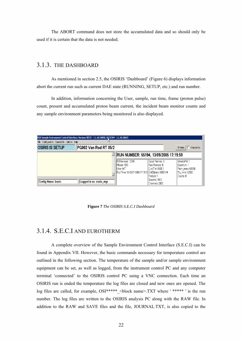
3.1.3. THE DASHBOARD

As mentioned in section 2.5, the OSIRIS ‘Dashboard’ (Figure 6) displays information

abort the current run such as current DAE state (RUNNING, SETUP, etc.) and run number.

In addition, information concerning the User, sample, run time, frame (proton pulse)

count, present and accumulated proton beam current, the incident beam monitor counts and

any sample environment parameters being monitored is also displayed.

Figure 7 The OSIRIS S.E.C.I Dashboard

3.1.4. S.E.C.I AND EUROTHERM

A complete overview of the Sample Environment Control Interface (S.E.C.I) can be

found in Appendix VII. However, the basic commands necessary for temperature control are

outlined in the following section. The temperature of the sample and/or sample environment

equipment can be set, as well as logged, from the instrument control PC and any computer

terminal ‘connected’ to the OSIRIS control PC using a VNC connection. Each time an

OSIRIS run is ended the temperature the log files are closed and new ones are opened. The

log files are called, for example, OSI*****_<block name>.TXT where ' ***** ' is the run

number. The log files are written to the OSIRIS analysis PC along with the RAW file. In

addition to the RAW and SAVE files and the file, JOURNAL.TXT, is also copied to the

23

analysis PC. JOURNAL.TXT contains a list (Date, Run No, Users, Title, Run Duration and

uamps) of all OSIRIS experiments performed to date.

In addition, data collection can be temporarily suspended when the temperature drifts

outside of a specified range. There are essentially three aspects to the temperature control

system. The control PC (for issuing the commands), the CAMAC unit (hardware/software

interface) and the Eurotherm temperature controllers. The temperature controllers measure

the millivolt output from resistance thermometers (Rh/Fe or Pt) or thermocouples (usually

type-K) and control the temperature at a specified set point using a 3-term control algorithm

(proportional band, integral time and derivative time - commonly referred to as PID control).

The conversion from millivolts to K or C is achieved using ‘look-up’ tables held on the

mainframe (each Rh/Fe sensor for example is calibrated at a number of points and has its own

conversion table and identification number). While the unit of temperature (K or C) depends

upon the sample environment equipment being used it would normally be Kelvin for a

cryostat and Celsius for a furnace. The ‘Dashboard’ usually displays both the millivolt

readings and the corresponding K or C value. TEMP1 and TEMP2 are examples of two

software temperature control blocks in S.E.C.I that correspond to the two EUROTHERM

temperature controllers.

3.1.6. TEMPERATURE CONTROL

Listed below are the more useful commands in the S.E.C.S relating to the control of

temperature: The controls are entered in the active Open Genie window.

CSET TEMP1=10 Sets temperature observed temperature control

block, TEMP1, to 10 K.

CSHOW TEMP1 Displays information about the current status of

TEMP1.

CSET/CONTROL TEMP1 = 15 LOWLIMIT = 10 HIGHLIMIT = 20

24

This command issues a set point value of 15 (K

or C) to temperature control block TEMP1. The

controller attempts to maintain a temperature of

15 +/- 5 (K or (C) as denoted by the ‘limits’.

LOWLIMIT and HIGHLOIMIT are used to

inhibit data collection because of the

/CONTROL prompt. If TEMP1 varies outside

this range OSIRIS go into the WAITING state

until the value returns into the range.

CSET/NOCONTROL TEMP1 Data collection vetoing is disabled if TEMP1

falls outside HIGHLIMIT or LOWLIMIT.

SETEURO1 P=1 D=1 I=1 Sets P.I.D values on Eurotherm controller No 1.

P=Proportional, I=Integral and D=Derivative

bands. Can also set max power (MP=100) and

auto tune (AT)

** Suitable P.I.D values for the different sample environment apparatus used on OSIRIS are listed in

Appendix IV

3.1.7. COMMAND FILES

Automatic control of OSIRIS can be achieved using a simple user written command

file. Based on OpenGenie code, command files are created using either Notepad or Wordpad

and saved as a .GCL file in the Users area on the U: drive. An simple example .GCL file is

given on the next page:

25

PROCEADURE Example

# Measure at T=1.5K on d-range 1 and T=10K on d-range 2

cset/control temp1=1.5 highlimit=3.0 lowlimit=1.0

drange 1

begin

change title = "An OSIRIS experiment at T=1.5K d1"

waitfor uAmps = 50

end

ENDPROCEADURE

To load a GCL command, type

LOAD “<file.gcl>”

into the active Open Genie window. A GCL command file will not run unless it loads into

Open Genie without error.

3.2. DATA VISUALISATION AND ANALYSIS

Data visualisation, and subsequent analysis, on OSIRIS utilises PC based software.

A brief description of the four main software packages, and links to further information, is

given below.

NOTE: DO NOT use the OSIRIS control PC for data analysis

3.2.1 DATA ANALYSIS AND REDUCTION SOFTWARE

• OPENGENIE

OPENGENIE is an ISIS developed data visualisation package common to all ISIS

instruments. It is used for displaying and manipulating spectra and data sets. A

comprehensive overview of OPENGENIE can be found at

http://www.isis.rl.ac.uk/OpenGENIE/

To start OPENGENIE click on the ‘OPENGENIE’ icon on the analysis PC desktop.

Useful data visualisation commands include (older GENIE syntax is also included):

26

GENIE v2 Command Open GENIE Command Description

a b N (N=1,2,3,…) a/b N alter binning

a m N a/m N alter markers

ass ass Assign

d/h/l/m/e d/h/l/m/e Display

l l Limits

m m Multiplot c/v/h c/v/h Cursor

ex ex Exit j “OS command” j “OS command” Jump

k/h k/h keep hardcopy

p/h/l/m/e p/h/l/m/e Plot reb reb Rebin

set disk my$disk set/disk “my$disk:” set disk

set dir [mydir] set/dir “[mydir]” set directory

set ext raw set/ext “raw” set extension

set inst ANY set/inst “ANY” set instrument set par setpar set wksp parameters

set title w1 w1.title= set title

sh data sh/data show data

sh par sh/par show parameters

sh def sh/def show defaults

u/? u/? Units

z z Zoom

• ARIEL

ARIEL is the preferred package for the reduction of diffraction data collected on

OSIRIS (i.e. reducing the data to GSAS, CCSL or some other portable format). ARIEL runs

under IDL. For details about how to use AREIL see:

http://www.isis.rl.ac.uk/disordered/gem/Software/Ariel3.1release.htm

27

• LAMP

LAMP is an alternative package for the reduction of diffraction data collected on

OSIRIS (i.e. reducing the data to GSAS, CCSL or some other portable format). LAMP runs

under IDL with a convenient syntax for manipulating neutron data. For details about how to

use LAMP see:

http://www.isis.rl.ac.uk/molecularspectroscopy/osiris/osiris_dataanalysis.htm

However, the LAMP code is no longer supported at ISIS and as a result this

package is to be superseded by ARIEL

• MOSES

MOSES is a suite of programs for the full reduction and analysis of OSIRIS

spectroscopy data. An online MOSES manual can be found at:

http://www.isis.rl.ac.uk/molecularspectroscopy/osiris/

A more in-depth descriptions of the individual analysis programs themselves can be

in the GUIDE and IDA manuals. These can be found online at:

http://sutekh.nd.rl.ac.uk/wsh/index.html

MOSES can be launched by typing clicking on the ‘MOSES' icon on the OSIRIS

analysis PC desktop

• MSLICE

MSLICE is a MatLab based analysis tool predominately used for the visualisation and

analysis of magnetic excitations. MOSES is used to convert the RAW data to a format that

can be read by MSLICE. Information about MSLICE can be found at:

http://www.isis.rl.ac.uk/excitations/index.htm

28

IV. REFERENCES

i) PUNCH user guide. R G Parry et al. RAL Report, RAL 88109 (1988).

ii) GUIDE – OSIRIS Data Analysis M.T.F.Telling and W.S.Howells RAL Report: RAL-

TR-2000-004, Jan 2000 (http://www-dienst.rl.ac.uk/library/2000/tr/raltr-2000004.pdf)

iii) GSAS user guides, software and information: http://public.lanl.gov/gsas/

iv) Cambridge Crystallography Subroutine Library (CCSL) information:

http://www.isis.rl.ac.uk/crystallography/documentation/CCSL/CCSLguideFra

mePage.htm

v) M.T.F.Telling and K.H.Andersen, Spectroscopic characteristics of the OSIRIS

near-backscattering crystal analyser spectrometer on the ISIS pulsed neutron

source, Phys Chem Chem Phys 7 1255-11261 (2005)

29

APPENDIX I - QUASI / IN ELASTIC SETTINGS.

Analyser

Fwhm (μeV)

ΔE

(meV)

Freq

Detector

TCB (μs)

Mon TCB (μs)

Mon

Bounds (μs)

Phases θ6.3/θ10

(μs)

Command

002

24.5

-0.4 to 0.4

50

51500.0 71500.0

45900.0 65900.0

58732.0 60732.0

8573 14250

PG002

“

“

-0.7 to 0.8

25

40200.0 80200.0

36800.0 76800.0

66177.0 68177.0

6052 11250

PG002_25Hz

“

“

-0.2 to 1.2

50

45500.0 65500.0

40400.0 60400.0

53055.0 55055.0

7500 12500

PG002_OFFSET

“

“

-0.7 to 0.1

50

58700.0 78700.0

52000.0 72000.0

65545.0 67545.0

9738 16166

PG002_OFFSET1

“

“

-1.0 to 0.1

25

57300.0 97300.0

49400.0 89400.0

64220.0 66220.0

8964 15211

PG002_OFFSET2_25Hz

“

“

-0.1 – 25.0

16.6

15000.0 75000.0

14000.0 75000.0

50817.0 52817.0

1500 2805

PG002_OFFSET3_16Hz

“

“

-0.05 to 2.0

50

40500.0 60500.0

35300.0 55300.0

48323.0 50323.0

6569 10861

PG002_OFFSET4

“

“

-0.3 to 1.0

50

48500.0 68500.0

43600.0 63600.0

48323.0 50323.0

8207 13502

PG002_OFFSET5

004

99

-3.0 to 4.0

50

22500.0 42500.0

19000.0339000.0

31291.0 33291.0

3717 5657

PG004

“

“

-2.0 to 7.0

50

20500.0 40500.0

16700.0 36700.0

29398.0 31398.0

3217 4904

PG004_OFFSET1

Table 1 Standard Quasi / In - elastic settings

30

APPENDIX II - DIFFRACTION SETTINGS.

The diffraction detectors are placed in a ring around the incident beam. They cover

the full range of scattering angles 2θ from 150º to 171º, providing a total solid angle coverage

of 0.67 steradians.

Figure 8: Diffraction modules as seen from the sample position

Module Detectors

1 3 - 122 2 123 - 242 3 243 - 362 4 363 - 482 5 483 - 602 6 603 - 722 7 723 - 842 8 843 - 962

The detectors are shown schematically above and as seen from the sample position.

They are scintillators and the full detector bank contains 8 modules, numbered according to

the order in which they were installed. Each module consists of 120 detector elements. The

first 20 are single detectors. Between 21 and 120 the even numbered detectors are still single

but the odd numbered are physically composed of one detector above and one below the

central strip, hardwired together, as shown for module 1 below.

31

Figure 9: Location of the 120 diffraction detectors in module 1

The choppers typically run at a frequency of 25 Hz, which allows a 4 Å wide

wavelength range to reach the sample with minimal contamination from other

wavelengths. The d-spacing measured are given by Bragg’s law: λ=2dsinθ and since the

diffraction detectors are close to backscattering (⇒ sinθ ≈ 1) the d-spacing is about half the

neutron wavelength. The range of d-spacing measured with the choppers at 25Hz is thus

about 2 Å wide. In order to measure a full range of d-spacing to properly characterise the

sample, a series of runs are usually performed with an incremental increase of the chopper

phasing. The data from these runs are then merged in software to create a data set that spans

the full range of d-spacing of interest in a continuous manner.

The combination of a cold moderator and a super mirror guide provides a high flux of cold

neutrons on OSIRIS. However, while neutron wavelengths of up to 70Å re accessible, 35Å is

the experimental limit. The reduction in flux at long wavelengths is partly compensated for by

the λ4 form factor that applies to Bragg peak intensities. The use of a super mirror guide

significantly enhances the neutron flux at all wavelengths, but at a price in beam divergence,

which increases substantially as a function of wavelength. This is why the diffraction

detectors on OSIRIS only cover the highest scattering angles, where beam divergence does

not contribute greatly to the instrumental d-spacing resolution. At Δd/d down to 2.5×10-3,

OSIRIS provides similar resolution to the HRPD 90° bank with the same counting rate as on

GEM. OSIRIS can reach d-spacings in excess of 30 Å with high resolution, but cannot access

d-spacing below about 0.9 Å, due to the curved guide cut off.

32

Total d-spacing

range (Å)

Ariel d-spacing

range (Å)

Q / Å-1 Time-channel-

boundaries (μ S)

Phases (μS)

θ6.3 / θ10

drange 1 0.70 - 2.90 0.7 – 2.5 8.9771 - 2.5136 11700 - 51700 1011/1566

drange 2 1.80 - 4.00 2.1 – 3.3 2.9924 - 1.9042 29400 - 69400 4599/7715

drange 3 2.90 - 4.90 3.1 - 4.3 2.0271 - 1.4614 47100 - 87100 7590/12859

drange 4 3.70 - 6.00 4.1 – 5.3 1.5327 - 1.1857 64800 - 104800 10407/17715

drange 5 4.90 - 7.00 5.2 – 6.2 1.2085 - 1.0135 82500 - 122500 13015/22800

drange 6 5.70 - 8.00 6.2 – 7.3 1.0135 - 0.8608 100200 - 140200 16100/27973

drange 7 7.00 - 9.00 7.3 – 8.3 0.8608 - 0.7571 117900 - 157900 19480/33251

drange 8 8.10 - 10.00 8.3 – 9.5 0.7571 - 0.6615 135500 - 175500 22571/38130

drange 9 8.70 - 11.00 9.4 – 10.6 0.6685 - 0.5928 153200 - 193200 26062/3609

drange 10 10.2 - 12.00 10.4 – 11.6 0.6042 - 0.5417 170900 - 210900 28953/8228

drange 11 10.80 - 13.00 11.0 – 12.5 0.5713 - 0.5027 188600 - 228600 32144/13367

/

Table 2 Standard Diffraction Settings at 25Hz

• drange is used to change chopper phases and load new time channel boundaries.

NB: include the string dN in the run title to enable Ariel to stitch the data sets together. For

example: “Aluminium d4 Room Temperature”

33

Figure 10: Low d-spacing background features observed when measuring i) the 5mm diameter

vanadium standard and b) the empty sample bin. The effect of coving the sample bin’s aluminium exit

window with gadolinium foil is also illustrated. Al = Aluminium, V = vanadium, Gd = gadolinium

34

APPENDIX III - INSTRUMENT PARAMETERS.

Operating vacuum: 2 x 10-6mb (instrument tank, analyser ON)

3 x 10-5mb (instrument tank, analyser OFF)

4 x 10-5mb (sample environment bin)

Primary instrument flight-path: L1 = 34.00 m

Inelastic:

Analysing energy (for graphite at 8K, PG002) 1.845 meV

Analysing energy (for graphite at 8K, PG004) 7.375 meV

Average secondary flight-path: L2 = 1.582 m

Angular coverage of 3He detector bank: 11° < 2θ <155°

Spectrum numbers: 963 to 1004

Diffraction:

Average secondary flight path: L 2 = 1.005m

Angular range of diffraction detectors: 167.1° < 2θ <172.4°

Resolution: . 5×10-3 < Δd/d < 6×10-3

Solid angle: 0.67 steradians

d-spacing range: 0.8 Å < d < ~35 Å

Spectrum numbers: 3 to 962

35

Figure 11: Momentum transfer vs. scattering angle for the OSIRIS pyrolytic graphite analyser bank.

The Q values are those calculated at the elastic line i.e. KI = KF Exact values are given in the table

below

36

Detector No.

Spectra Number

2θ (degrees)

Q Value (002)

Q Value (004)

963 963 11.50 0.18 0.37

964 964 14.82 0.24 0.48

965 965 18.15 0.29 0.59

966 966 21.48 0.35 0.69

967 967 24.81 0.40 0.80

968 968 28.14 0.45 0.91

969 969 31.47 0.51 1.01

970 970 34.80 0.56 1.12

971 971 38.17 0.61 1.22

972 972 41.46 0.66 1.32

973 973 44.79 0.71 1.43

974 974 48.12 0.76 1.53

975 975 51.45 0.81 1.62

976 976 54.78 0.86 1.72

977 977 58.10 0.91 1.82

978 978 61.43 0.96 1.91

979 979 64.76 1.00 2.01

980 980 68.09 1.05 2.10

981 981 71.42 1.09 2.19

982 982 74.75 1.14 2.27

983 984 78.08 1.18 2.36

984 984 81.41 1.22 2.44

985 985 84.74 1.26 2.52

986 986 88.07 1.30 2.60

987 987 91.40 1.34 2.68

988 988 94.73 1.38 2.76

989 989 98.06 1.42 2.83

990 990 101.30 1.45 2.90

991 991 104.71 1.49 2.97

992 992 108.04 1.52 3.03

993 993 111.37 1.55 3.10

994 994 114.70 1.58 3.16

995 995 118.03 1.61 3.21

996 996 121.36 1.64 3.27

997 997 124.69 1.66 3.32

998 998 128.02 1.69 3.39

999 999 131.35 1.71 3.42

1000 1000 134.68 1.73 3.46

1001 1001 138.01 1.75 3.50

1002 1002 141.34 1.77 3.54

1003 1003 144.67 1.79 3.57

1004 1004 148.00 1.81 3.60

37

APPENDIX IV - P.I.D PARAMETERS

PROP = PROPORTIONAL BAND

INT = INTEGRAL TIME

DERIV = DERIVATIVE TIME

** AS TEMPERATURE INCREASES ‘INT’ AND ‘DERIV’ SHOULD BE PROGRESSIVELY DECREASED BUT

KEEPING TO A 6:1 RATIO

Orange Cryostat Temp (K) 1 – 5 5 – 10 10 – 20 20 - 300

Prop (%) 3 3 1 1

Int (s) 1 10 10 50

Deriv (s) 0.17 1.67 1.67 8.3

Orange Cryostat (control on the sample) Temp (K) 1 - 20 20 - 50 50 - 100 150 - 300

Prop (%) 2 2 2 2

Int (s) 40 100 200 999

Deriv (s) 6.7 16.7 33.3 166.5

CCR Temp (K) 10 – 50 50 – 150 150 –300

Prop (%) 2 2 2

Int (s) 50 100 200

Deriv (s) 8.3 16.7 33.3

38

APPENDIX V - OUT OF HOURS SUPPORT

Normal working hours for most ISIS staff (apart from the ISIS crew who are on shift

duty) are from 08:30 to 17:00 (Mon to Fri). Outside these hours most local contacts at ISIS,

including many members of the technical support groups, voluntarily agree to provide some

form of out-of-hours User support. The first point of call (after this manual) should be the

Local Contact for the experiment, assistance being available during ‘reasonable’ hours. The

definition of ‘reasonable’ depends upon the individual concerned. However, as a general rule,

for local contacts on OSIRIS and members of the technical support groups, the hours between

08:00 and 23:00 would probably be deemed reasonable. Unless it has been agreed that a

person may be contacted outside of these hours then the following procedure should be

adopted:

i) Check the manual for possible solutions and explanations.

ii) Investigate whether the problem can be put off until a more reasonable time e.g.

can the experimental timetable can be adjusted by, perhaps, performing a

background or a resolution measurement?

iii) Is a member of the ISIS crew able to assist with the problem?

iv) If none of the above apply ensure that the experimental set-up is safe (the ISIS

duty officer in the MCR will advise if necessary) and wait until a more

reasonable time. Loss of beam time due to ISIS/OSIRIS/Sample Environment

problems is always dealt with sympathetically and, if appropriate, the lost beam

time will be is rescheduled at a later date.

39

APPENDIX VI - USEFUL TELEPHONE NUMBERS

General:

Accident/Emergency/Fire 2222

Health Physics (Radiation) 6696

ISIS Main Control Room (MCR) 6789

OSIRIS Cabin 6896

Main gate (Security) 5545

Computer support 1763

Office numbers:

Dr Mark Telling 5529

Dr Vicky Garcia-Sakai 6703

Dr Felix Fernandez-Alonso 8203

Dr Franz Demmel 8283

40

APPENDIX VII. – USEFUL DIAGRAMS

41

42

43

44

45

CAD drawing numbers for 50 mm x 40 mm OSIRIS flat plate sample cans

Flat plate (csk) Common to assemblies Si-4206-307 Window frame 0.1 mm Si-4206-308 Window frame 0.2 Si-4206-309 Window frame 0.3 Si-4206-310 Window frame 0.4 Si-4206-311 Window frame 0.5 Si-4206-312 Window frame 1.0 Si-4206-313 Window frame 2.0 Si-4206-314

CAD drawing numbers for 50 mm x 26 mm OSIRIS flat plate sample cans

Flat plate (csk) Common to assemblies Si-4206-322 Window frame 0.1 mm Si-4206-323 Window frame 0.2 Si-4206-324 Window frame 0.3 Si-4206-325 Window frame 0.4 Si-4206-326 Window frame 0.5 Si-4206-327 Window frame 1.0 Si-4206-328 Window frame 2.0 Si-4206-329

46

APPENDIX VIII - S.E.C.I INFORMATION

INTRODUCTION

The Sample Environment Control Interface (S.E.C.I) programme’s main role is to

manage the instrument control software; essentially, S.E.C.I is responsible for organising and

displaying the software that actually runs the experiment, such as Labview etc. S.E.C.I was

developed in-house at ISIS in an attempt to meet the unique requirements of the experiments

carried out on-site.

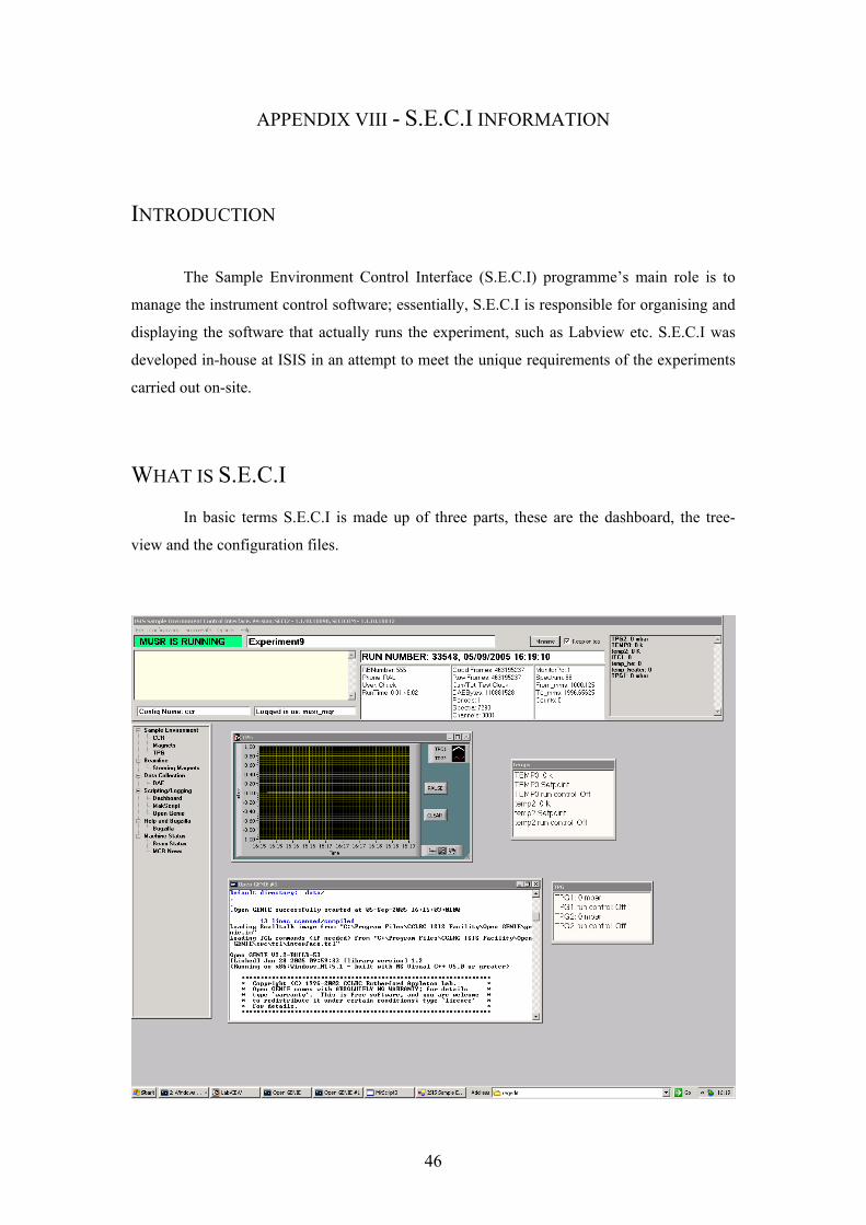
WHAT IS S.E.C.I

In basic terms S.E.C.I is made up of three parts, these are the dashboard, the tree-

view and the configuration files.

47

The dashboard appears at the top of the screen and provides an overview of the

instrument status. The dashboard itself is divided up into three main parts (from left to right):

• The error box - any errors that occur in the experiment are listed in this box

• The main status panel - lists a number of experimental values (examples: run-time,

beam current, number of counts etc) which are updated every two seconds.

• The block list – this area can be customised to list experimental values which are not

included in the main status panel.

The tree-view groups the experiment in to manageable pieces, which can be viewed

separately from each other. By selecting the appropriate node on the tree, S.E.C.I hides all the

other nodes and only displays the selected one. The contents of the nodes are customisable,

for example: all the control panels for the experiment can be grouped under one node or

alternatively, they could be grouped by type or even individually.

The configuration files are text files that are used to set-up S.E.C.I for different

experiments or instruments. The configurations are created by the instrument scientists

through S.E.C.I. The configuration file principally determines which nodes are available in

the tree-view, which programmes populate these nodes and which – if any – experimental

values are listed in the block list.

USING S.E.C.I

ACCOUNTS

The File menu is used for adding or removing user accounts and for logging in or out.

To log in you must have an S.E.C.I account and know the relevant password. There are three

types of account (in order of power): Administrator, Instrument Scientist and User. Of these,

the user and instrument scientist accounts are the most used.

48

The Administrator accounts have the following privileges:

• Create Administrator, Instrument Scientist and User accounts.

• Remove instrument scientist and user accounts.

• Overwrite or delete configurations saved by Administrators, Inst Sci,Users.

• Open any saved configuration.

• Create new configurations.

• Edit configurations and save them under a different filename.

• Minimise S.E.C.I.

The Instrument Scientist accounts have the following privileges:

• Overwrite or delete configurations saved by Instrument Scientists and Users.

• Open any saved configuration.

• Create new configurations.

• Edit configurations and save them under a different filename.

• Minimise S.E.C.I.

The User accounts have the following privileges:

• Overwrite or delete configurations saved by other Users.

• Open any saved configuration.

• Create new configurations.

• Edit configurations and save them under a different filename.

To add an account, select ‘Add User’ from the File menu (Administrator only). In the

dialog panel enter in the new account name and password, then select the type of account

required and click ‘OK.’ The new account is now added to the account database. Note: this

account will be valid for all instruments.

To remove an account, select ‘Remove User’ from the File menu (Administrator

only). In the dialog panel select the group of the user and then the user’s name from the list.

To delete the account click ‘OK.’

49

CONFIGURATIONS

As stated previously, configurations are used to configure S.E.C.I for different

experimental set-ups. They determine which programmes S.E.C.I loads (Labview,

OpenGENIE and so on), which initial values equipment take, and which nodes are available

on the tree-view. Through S.E.C.I it is possible to open different configurations, modify

existing configurations and create new configurations.

OPENING A CONFIGURATION

To open a configuration it is necessary to be logged in with a valid account. From the

Configuration menu select ‘Open Configuration,’ this will open a dialog form which lists all

the available configurations for the current instrument. From the list select the required

configuration and click ‘OK,’ S.E.C.I will now shutdown and restart in the new configuration.

This may take a minute or so.

ADDING A DISPLAY PAGE (A TREE-VIEW NODE)

To add a node to the tree-view, select ‘Display Pages’ from the Configuration menu

then from the sub-menu select ‘Add Display Page.’ A ‘New Display Page’ dialog form will

now be shown. The top list box shows the main nodes, the new page will be a sub-node of

one of these nodes. From the list of nodes select the required node, next it is necessary to

name the new sub-node. Finally, it is necessary to choose the page type, the options are:

• VI – this is short for Virtual Instrument, this means the display page will be used for

displaying Labview panels.

• Web – the page will be used for displaying web-pages

• Other – the page will be used other kinds of programmes.

Next, click ‘OK,’ the new page should now appear as a sub-node of one of the main nodes.

To make this change permanent the configuration will need to be saved.

50

REMOVING A DISPLAY PAGE

Firstly to remove a Display page it is necessary to remove any programmes (see

section 0) or Labview panels (see sections 0 and 0) from the page first. Then select ‘Display

Pages’ from the Configuration menu then from the sub-menu select ‘Remove Display Page.’

From the new window select the display page to remove then click ‘OK.’ The page should

now be removed, to make this removal permanent it is necessary to save the configuration.

RENAMING A DISPLAY PAGE

To rename an existing Display page select ‘Display Pages’ from the Configuration

menu then from the sub-menu select ‘Rename Display Page.’ From the new window select

the Display page to rename and then enter a new name, to finish click ‘OK.’ The Display

name will now have been changed, to make this change permanent the configuration must be

saved.

ADDING A LABVIEW PANEL TO AN EXISTING CONFIGURATION

To add a Labview panel to a configuration, it is necessary to have a node on the tree-

view for Labview panels, to do this see section 0.

To add a Labview panel select ‘Labview Panels’ from the Configuration menu and

from the sub-menu select ‘Add Labview Panel.’ A new ‘Add Labview’ dialog panel will open

from which the display page for the new Labview panel can be selected. When a display page

is chosen a File dialog box will open, from this select the desired Labview VI file and click

‘Open.’ The location of the new VI file will now be listed in the ‘Add Labview’ dialog panel,

click ‘Add’ to add the new Labview panel. A new dialog panel will open; from this dialog

panel it is possible to configure the behaviour of the Labview panel. The first option is

whether to add any associated INI files to the Labview panel. The INI files contain data for

initialising and configuring the Labview panels. The two other options available for the new

Labview panel are whether to start the panel running upon loading or to hide the panel. The

configuration will need to be saved to make this change permanent.

51

REMOVING A LABVIEW PANEL FROM EXISTING CONFIGURATIONS

To remove a Labview select ‘Labview Panels’ from the Configuration menu and

from the sub-menu select ‘Remove Labview Panel.’ A dialog panel will open; from this panel

select the Display page from which the Labview panel will be removed and then select the VI

to remove. Click ‘OK’ and the panel is removed from this instance of the configuration. The

configuration will need to be saved to make this change permanent.

CHANGING A LABVIEW PANEL’S ASSOCIATED FILES

From the Configuration menu select ‘Labview Panels’ and then select ‘Change

Associated files’ from the sub-menu. A new dialog window will open, from this select the

Display page of the Labview panel to be edited and then select the actual VI. It is now

possible to add or delete the associated INI file for the panel. To make any changes

permanent the configuration will need to be saved.

MOVING A LABVIEW PANEL TO A DIFFERENT DISPLAY PAGE

First it is necessary to select the Display page containing the Labview panel which is

to be moved. Then from the Configuration menu select ‘Labview Panels’ and then select

‘Move Labview Panel to Another Page’ from the sub-menu. The new window will list the

Labview panels available in the selected Display page, select the panel to move then choose

which Display page to move it to. Click ‘OK’ and the Labview panel will now be shown on

the chosen Display page. To make the change permanent the configuration will need to be

saved.

EDITING THE START-UP ORDER OF THE LABVIEW PANELS

The behaviour of one Labview panel may depend on one or more other Labview

panels, and subsequently the order in which the panels are loaded may be of significance. To

set the start-up order of the panels select from the Configuration menu ‘Labview Panels’ and

then choose ‘Set Properties for Panels’ from the sub-menu. A new window appears

containing a chart of the Labview panels in the configuration. In this chart it is possible to set

52

the order in which the Labview panels are loaded. Each panel must have a unique value for

the order. Any panels that have not been explicitly set an order number will be assigned an

order number greater than 10,000 by S.E.C.I. It is also possible to set a wait time for each

panel, this indicates how long after the previous panel has loaded should the panel wait before

loading. Once any editing has been completed click ‘OK’ to finish. To make any changes

permanent it is necessary to save the configuration.

SETTING THE VISIBILITY OF THE LABVIEW PANELS

It is possible to hide Labview panels when the user does not need to know about

them. The visibility of all the panels can be edited or reviewed in one window. To do this,

select from the Configuration menu ‘Labview Panels’ and then choose ‘Set Properties for

Panels’ from the sub-menu. A new window will appear (the same as in section 0). The

checkboxes in the ‘Visible?’ column show whether a panel is visible or not – checked for

visible, unchecked for not. The visibility of a Labview panel can be set by clicking on the

checkbox. When finished click ‘OK’ to close the window. The configuration will then have to

be saved to make any changes permanent.

SETTING A LABVIEW PANEL TO RUN AUTOMATICALLY

Labview panels can be set to run automatically after loading or not when S.E.C.I.

This property is set in the same window as discussed in sections 0 and 0. To open this

window, select from the Configuration menu ‘Labview Panels’ and then choose ‘Set

Properties for Panels’ from the sub-menu. In the new window there is a column called ‘Run at

Start-up?’ If the checkbox is checked for a Labview panel then it will start running when it is

loaded, if it is unchecked then it will load but will require the user to start it. By clicking the

checkbox this setting can be changed from on (checked) to off (unchecked). Click ‘OK’ to

keep the changes and close the window. To make these changes permanent the configuration

will need to be saved.

ADDING NON-LABVIEW PROGRAMMES TO CONFIGURATIONS

To add non-Labview programmes to a configuration it is necessary to add a Display

page for these programmes as shown in section 0. If this has been done then select ‘Other

53

Programmes’ from the Configuration menu, in the sub-menu select ‘Add Programme.’ In the

new window select the Display page to add the new programme to this will open a file dialog

window for selecting the new programme. Choose the programme to add then click ‘Open,’

this will close the file dialog window. Click ‘Add’ and the new programme will be added to

the Display page. The configuration will need to be saved to make this change permanent.

REMOVING OTHER PROGRAMMES

To remove a non-Labview programme from a configuration select ‘Other

programmes’ from the Configuration menu, in the sub-menu select ‘Remove Programme.’ In

the new window select the Display page of the programme to be removed then select the

actual programme. Click ‘OK’ to remove the programme. The configuration will then need to

be saved to make this change permanent.

ADDING A WEB VIEWER TO A CONFIGURATION

To add a web viewer to a configuration it is necessary to add a Display page for web

pages as discussed in section 0. Then select ‘Web Viewers’ from the Configuration menu, in

the sub-menu choose ‘Add Web Viewer.’ In the new form select the Display page to add the

viewer to and then type in the URL of the web-site to display. Finally, enter a title for the web

viewer window and click ‘Add.’ The new web viewer should now appear. To add this web

viewer permanently the configuration will need to be saved.

REMOVING A WEB VIEWER

To remove a web viewer, first select the Display page with the web viewer in. Then

select ‘Web Viewers’ from the Configuration menu, in the sub-menu choose ‘Remove Web

Viewer.’ From the dialog box select the web viewer to remove and click ‘OK.’ To remove

this viewer permanently the configuration will need to be saved.

54

SAVING, VIEWING AND DELETING CONFIGURATIONS

The options to save, view and delete configurations are all grouped together under the

‘Save/Delete/View Configurations’ option on the Configuration menu. Choosing this will

open a new window offering the choices for saving, viewing and deleting configurations.

There are three different options for saving a configuration, these are:

• Save Current Config – this will save the current configuration without changing the

configuration name (i.e. it will overwrite the configuration). This is permission based, for

example: a User use ‘Save Current Config’ is the current configuration was created or saved

by an Instrument Scientist.

• Save Current Config As – this will enable the current operator to save the current

configuration under a different or new name. Again this is permission based: a User would be

able to save a configuration under a new name, but may not be able to save over an existing

configuration.

• Save As Other User – this allows an Instrument Scientist or Administrator to save the

current configuration as a lower permissions group. For example: an Instrument Scientist

could save a configuration as a User, thus the User will be able to overwrite the configuration.

To use ‘Save Current Config,’ click that button; the configuration will then be saved

depending on the permissions. To use ‘Save Current Config As,’ click that button, the

window will then change. In the changed window either enter in a new configuration name or

select an existing one, then click ‘OK.’ The configuration will then by saved if the

permissions are correct.To use ‘Save As Other User,’ click that button, the window will then

change. In the changed window either enter in a new configuration name or select an existing

one. Then select the permission group and username with which the configuration is to be

saved. Finally, click ‘OK’ and the configuration will be saved provided the permissions are

right.

Viewing a configuration allows the operator to view the Labview panels in a chosen

configuration. To do this click the ‘View A Config’ button, this will change the window. In

the changed window select the configuration to be viewed, after a few seconds the list of

Labview panels will be displayed. Click ‘OK’ to exit.

55

Deleting a configuration allows the operator to delete a chosen configuration.

Clicking the ‘Delete A Config’ button changes the window form, then from the changed form

select the configuration to be deleted and click ‘OK.’ The configuration will then be deleted

provided the current operator has the correct permissions to delete the chosen configuration.

ADDING ONE CONFIGURATION TO ANOTHER

It is possible to add one configuration to the current configuration. To do this, from

the Configuration menu select ‘Add Configuration’ this will open a window with a list of

available configurations. From the list select a configuration and click ‘OK,’ the chosen

configuration should now get added to the current configuration. The new combined

configuration will have to be saved for the changes to be permanent.

CLOSING THE CONFIGURATION

Selecting ‘Close Configuration’ from the Configuration menu will cause the current

configuration to be closed and the current operator to be logged out.

S.E.C.I OPTIONS

ADDING OR EDITING CUSTOM BLOCKS AND LOG VALUES

S.E.C.I allows the operator to customise the dashboard so that it can monitor

experiment values (known as blocks) which are not included in the main status panel. These

blocks are added via the ‘Monitor and Log Values’ option on the Options menu. Selecting

this option opens a new window form which contains a grid containing the current blocks.

Select an existing block and click ‘Change’ to edit it or click ‘Add’ to create a new block,

both methods will cause a new windows form to appear. This new form allows the block to be

configured, it is recommended that when configuring a new block to start from the top-left

and work down to the bottom right. This guide will provide a walkthrough for creating a new

block starting from the top-left:

56

1. Choose a Display page from the available Labview Display pages; this will create a

list of the panels (VIs) available.

2. From the list of panels choose the panel which contains the value to be monitored.

Once a panel has been chosen, the three lists on the next row down will be populated.

3. The first list (working from left to right) contains all the values (and their type, i.e.

Boolean, integer etc.) that can be monitored on the chosen panel. Highlight the

required variable to continue.

4. (Optional) The second list allows a set variable to be assigned. This allows

OpenGENIE to send new values for this variable to the Labview panel.

5. (Optional) If a set variable is assigned it may be necessary for OpenGENIE to push a

Labview button to send the new value. The third list chooses which button to press.

6. A name for the block must be entered and the option to include is also available.

7. The next three parameters to set are the frequencies for logging the block values and

for updating the blocks in the dashboards. This is done by setting the intervals, in

seconds, which S.E.C.I will wait before logging the value or updating the dashboard.

A value of zero will mean that the logging or updating will be disabled.

8. The next option is to decide whether to turn ‘Run Control’ on, by default it is off. Run

control determines a range of values between which data is collected, for example: if

there was a temperature block, it may be possible that only data for temperatures

between 10°C and 20°C needs to be recorded.

9. There is an option to save the block value (toggle on or off), this is for when a block

does not change during the experiment, rather than logging an unchanging value, the

value of the block is saved once at the end of the run. (THIS CURRENTLY DOES

NOT WORK AS S.E.C.I DOESN’T KNOW WHEN AN EXPERIMENT ENDS!)

10. The final option is to enable or disable the block. If the block is disabled it will no

longer log or update the values. The dashboard will still show the block name but

with disabled written next to it. When the block has been configured, click ‘OK’ to

finish.

57

Blocks can also be deleted; to do this select the block in the grid and then click

“Delete.” The order in which blocks appear on the dashboard can also be set by clicking

“Change Order.” This will open a new window in which the all the blocks are listed. By

selecting a block and clicking the “Up” or “Down” button the block’s position can be

changed, as required. Click “OK” to accept the changes. To make any changes permanent it is

necessary to save the configuration.

DASHBOARD PAGE OPTIONS

This section refers to the dashboard page node of the tree-view, not the S.E.C.I

dashboard. To access the Dashboard page options, select ‘Dashboard Page Options’ from the

Options menu. This will opened the Dashboard options window; from this window the

following options are available:

• Add A Graph – this option sets up a graph plot to monitor a block value

• Change A Graph –allows the properties of an existing graph to be changed.

• Delete A Graph – this option will remove an existing graph from the Dashboard page.

• Show or hide the big dashboard – choose whether to show the big version of the

S.E.C.I dashboard on the Dashboard page.

• Show or hide the OpenGENIE scripting window – choose whether to add the

OpenGENIE scripting window to the Dashboard page

• Add A Block Display Box – this option will add a window box to the Dashboard

page which contains the value(s) for a chosen block or blocks.

• Change A Block Display Box – this option allows the properties of an existing

display box to be changed.

• Delete A Block Display Box – this option will remove an existing display box from

the Dashboard page.

58

When ‘Add A Graph’ is selected a new window opens, from this window select the

block to be plotted. Next, choose whether to plot the set point then enter a label for the Y-axis

and a name for the graph. Finally, choose whether to show another block on the same graph

and whether to increase or decrease the graph buffer size (the number of points stored). Click

‘OK’ to add the graph. Choosing ‘Change A Graph’ will open a new window, in this window

all the values set for the graph when adding the graph can be changed. Click ‘OK’ to accept

the changes. Selecting ‘Delete A Graph’ will open a window listing the existing graphs.

Select the graph to delete and click ‘OK.’ The graph will now be deleted.

When ‘Add A Block Display Box’ is selected a new window opens, first add a name

for the new display box and then choose which blocks to add to the box. To select a block to

add, choose the block from the list then click ‘Add Selected Block Now.’ If a wrong block is

added it can be removed by selecting it in the ‘Blocks To Be Displayed’ list and click

‘Remove Selected Block.’ When all the required blocks have be added click ‘OK’ to create

the display box. Choosing ‘Change A Block Display Box’ will open a new window. In this

window select the display box to be added, then blocks can be added or removed from this

box. Click ‘OK’ when finished to accept the changes. Selecting ‘Delete A Block Display

Box’ will open a new window. In the list of display boxes chose the box to be deleted and

click ‘OK’ to delete it.

For all the options in the ‘Dashboard Page Options’ it is necessary to save the

configuration afterwards to make the changes permanent.

LOGGING DISPLAY VALUES

It is possible to log the values listed in the main status panel. To do this, select ‘Log

Display Values’ from the options menu. A new dialog window will appear, in this window

select the value to log and click ‘Add.’ This can be repeated for as many values as required.

Click ‘OK’ when finished. The values will now be logged every 10 seconds in

C:\data\InstName_RunNum_ValueName.txt.

WEB/WAP DASHBOARD OPTIONS

The status of an experiment being run by S.E.C.I can be viewed on the web, either

through a standard internet browser or a WAP equipped mobile phone can be used. However,

59

there may be occasions when an experiment is of a sensitive nature and the user wants to limit

the web access. There are two web options that can be enable or disabled on S.E.C.I:

• Display web dashboard (by default this is enabled). This option sets whether the web

dashboard will show any information on the web/WAP page.

• Show title (by default this is disabled). This sets whether the title is shown on the

web/WAP page. Thus it is possible to display the experiment status (which anyone

can see) for remote viewing but not the title which may contain sensitive information.

These options can be set under ‘Web/WAP Dashboard Options’ in the ‘Options’

menu by checking the choices on the sub-menu. These settings are stored in the S.E.C.I.ini

file.

S.E.C.I.INI SETTINGS

There are number of options in S.E.C.I that can only be configured using the

S.E.C.I.ini file. These options are:

• last_user_config – this keeps a record of the last configuration used\set before S.E.C.I

was closed. S.E.C.I will automatically load this configuration on start-up. If a

configuration causes S.E.C.I to crash on starting then a different configuration can be

set here.

• username_file – this sets which user file is used to check passwords against. This

should never need to be changed.

• last_run_number – this records the last run number before S.E.C.I was closed. This

should never need to be changed.

• status_colours – this determines whether the status colours on the S.E.C.I dashboard

are activated. It must be set to true or false.

• last_user – this keeps a record of who was logged in when S.E.C.I was closed.

S.E.C.I will start with this user logged in.

60

• UseNewDAE – some instruments are using a newer version of the DAE software,

this Boolean determines whether this is the case.

• RunningICP – this Boolean determines whether ICP is being run.

• IsMuons – this Boolean is used to set whether the experiment is a Muon experiment.

If this is true then the monitor values are not shown on the S.E.C.I dashboard.

These options should only be changed if you are certain you know what you are

doing.

S.E.C.I EXAMPLES

CREATING A SIMPLE CONFIGURATION

In this example a simple dummy configuration will be created. Starting from a blank

configuration (no extra pages or Labview panels):

1. Select Configurations->Display Pages->Add Display Page. In the new window:

• Select Instrument as the Page Group.

• Type in ‘Eurotherm Page’ as the Display Name to Create.

• Choose ‘VI’ as the page type.

• Click ‘OK.’

2. Select Configurations->Labview Panels->Add Labview Panel. In the new window do

the following:

• Choose ‘Eurotherm Page’ as the display page.

• In the file dialog window navigate to ‘Muon Eurotherm Front Panel,’ in this

directory select ‘Eurotherm Front Panel.vi’ and click ‘Open.’

61

• Click ‘Add’ and a new window opens. Select ‘Run VI When Loaded’ and

click ‘OK.’ The Labview panel should now appear.

3. Repeat 1 but call the new page ‘ITC Page.’

4. Repeat 2 but for the ‘ITC Page and navigate to the ‘SOLOITCFRONTPANEL’

directory in the ‘Oxford Software’ directory and choose ‘SoloITC503 – 2.vi.’ Again,

select ‘Run VI When Loaded.’

5. For this example it is necessary that the SoloITC503 – 2.vi always loads first. Select

Configuration->Labview Panels->Set Panels Startup Order. A new window will

appear with the two VIs listed, change the order for the SoloITC503 – 2.vi from

10001 to 1 and click ‘OK.’

6. It is decided that it would be useful to display the Sample temperature from the

Eurotherm panel on the S.E.C.I dashboard. It is also required that the values are

logged in a text file. From the Options menu select ‘Monitor and Log Values’ a new

window will open. Click the ‘Add’ button and do the following (starting from the

top-left):

• Choose ‘Eurotherm Page’ from the list of display pages then select the VI.

• Select ‘Sample Temperature (Numeric)’ from the ‘Value to Read’ list.

• Ignore the optional parameters and enter ‘Sample_Temp’ as the name and K

as the units

• Leave the remaining settings as their default values and click ‘OK,’ then click

‘OK’ again to close the final window. The Sample Temperature should now

be displayed in the dashboard and be logged in c:\data\.

7. It is now decided that plotting a graph of the Samp_Temp on the Dashboard page

would be useful, to do this:

• Select Option->Dashboard Page Options.

62

• In the new window, click ‘Add A Graph.’

• Choose the Sample_Temp block and enter ‘Temperature’ for the Y-axis

name and Sample_Temp for the graph name. Then click OK. The graph

should now appear on the Dashboard page of the tree-view.

A simple configuration has now been created and this can be saved. Warning: do not

use this configuration on an instrument as it is only an example.

63

APPENDIX IX - COMMAND LINE SCRIPTING

Scripting on the PC is done via an Open GENIE window. The command style is very

similar to the VMS operating system i.e:

COMMAND/QUALIFIER value1 value2 keyword1=value3 keyword2=value4

For example:

CHANGE title=”new title” user=”new user”

CSET/WAIT temp1=4.0

There are a few important differences from VMS however. Character strings must

always be included in “” quotation marks – this is to distinguish them from words or

functions that form part of the GENIE language and so make interpreting the language easier

to program. For example, on VMS you could type:

CHANGE title something ! Works on old VMS system only

This was possible because a separate program interpreted each command – with the

GENIE processor we need to tell it that title and something are not variable names. Being

more explicit in this way allows more complicated expressions to be written in the language.

For example in GENIE you can change both the title and user in one command as shown

above.

In moving commands from VMS to the PC, commands will usually become of the

form name=value. A list of PC commands and their VMS alternative are tabulated below:

64

PC Command

(syntax / example)

Equivalent VMS

Command

Action

CHANGE title=String

CHANGE title=”new title”

CHANGE title something

CHANGE title “””new title”””

Change the current run title

CHANGE user=String

CHANGE user=”new user”

Changes the current user(s)

CHANGE rbno=Integer

CHANGE rbno=1236

Changes experiment RB

number

UPDATESTORE

UPDATE followed by STORE

Created a SAV file which is

copied to the analysis PC

CHANGE period=Integer

CHANGE period=2

CHANGE period 2

WAITFOR uamps=Real

WAITFOR uamps=5.3

WAITFOR 5.3 uamps

Sets number of uamps to

wait for

WAITFOR frames=Integer

WAITFOR frames=4000

WAITFOR seconds=Integer

WAITFOR seconds=10

WAIT 00:00:10

PC control waits for N

seconds before continuing

END

END

Creates RAW files and

copies it to analysis PC

65

PAUSE

PAUSE

RESUME

RESUME

ABORT

ABORT

CSHOW block_name

CSHOW temp1

CSHOW temp1

CSET block=value

CSET temp1=5.0

CSET temp1 5.0

CSET/CONTROL

block=value lowlimit=low

highlimit=high

CSET/CONTROL temp1=5.0

lowlimit=4.8 highlimit=5.2

Command files or control scripts can be run from an Open GENIE window on the

instrument computer. A script is basically a compiled Open GENIE procedure, which is

executed in the window. A procedure can be loaded in one of two ways depending on how it

is written.

(1) You can write a standard PROCEDURE … ENDPORCEDURE program … in which

case you use the LOAD or INCLUDE command

(2) You write a section of one line commands, in which you use the loadscript command.

The LOADSCRIPT command will take the command, wrap them in a

PROCEDURE … ENDPORCEDURE with the procedure name the same as the

filename passed to LOADSCRIPT

66

Whichever you use, you will get a command which you can type to begin running the

file. Procedure commands include all standard open genie commands with the following

additions:

BEGIN # start data collection

END # stop data collection

PAUSE

RESUME

UPDATESTORE # create a SAV file from the DAE

CHANGE title=String # e.g. CHANGE title=”new title”

CHANGE user=String # e.g. CHANGE user=”new user”

CHANGE period=Integer # e.g. CHANGE period=3

CHANGE rbno=Integer # e.g. CHANGE rbno=12345

WAITFOR frames=Integer

WAITFOR unames=Real

WAITFOR seconds=Ineger

WAITFOR time=

PUSHLABVIEWBUTTON “vi name” “button name” # push this button on a VI

PUSHLABVIEWBUTTON/WAIT “vi name” “button name” # push this button on a VI and

wait for it to pop back up

Value=GETLABVIEWVAR(“vi name”,“variable name”)

SETLABVIEWVAR “vi name” “variable name” value

CSHOW/ALL

CSHOW block

CSET block=value lowlimit=value range:low:high highlimit=value

CSET/WAIT block=value # wait for in range

CSET/CONTROL block

CSET/DISPLAY block

GETRUNSTATE() # function to return run state e.g. “SETUP”

WAITFORBOOLEAN/TRUE “vi name” “Boolean variable name”

WAITFORBOOLEAN/FALSE “vi name” “Boolean variable name”

WAITFORBUTTON “vi name” “button name” # wait for button to pop up

Note: do not create a variable with the same name as a CAMAC block

67

COMMAND FILE EXAMPLES:

Example 1

cset/control temp1=300.0 lowlimit=295.0 highlimit=305.0

cset/wait temp1=300.0 lowlimit=295.0 highlimit=305.0

cset wccr -150.0

change title="thiourea parabanic acid 300 K wccr=-150 Tilt OR2 j:15,10"

begin

sleep 60

waitfor uamps=30.0

updatestore

waitfor uamps=200.0

end

#

Example 2

PROCEDURE SXD_SUB

PARAMETERS ccr_val t1

LOCAL tmp

setlabviewvar "sxd ccr - front panel.vi" "Target" ccr_val

pushlabviewbutton "sxd ccr - front panel.vi" "Move"

LOOP

tmp = getlabviewvar("sxd ccr - front panel.vi", "Ready")

EXITIF tmp = 1

printin "waiting for ccr"

SLEEP 5

ENDLOOP

cset temp1=t1

LOOP

tmp = getlabviewvar("eurotherm controller - details.vi", "Temperature - 0")

EXITIF (abs(t1 - tmp) <= 20)

printin "waiting for eurotherm"

SLEEP 5

ENDLOOP

68

ENDPROCEDURE

#

PROCEDURE SXD_SCAN

sxd_sub -155.0 300.0

begin

waitfor uamps=60.0

end

sxd_sub -120.0 300.0

begin

waitfor uamps=60.0

end

printin "Finished"

ENDPROCEDURE

#