Embed Size (px)
Citation preview

ORNL/CON-343
THE ORNL MODULATING HEAT PUMPDESIGN TOOL — MARK IV USER’SGUIDE
C. K. Rice

DOCUMENT AVAILABILITY
Reports produced after January 1, 1996, are generally available free via the U.S. Department ofEnergy (DOE) Information Bridge:
Web site: http://www.osti.gov/bridge
Reports produced before January 1, 1996, may be purchased by members of the public from thefollowing source:
National Technical Information Service5285 Port Royal RoadSpringfield, VA 22161Telephone: 703-605-6000 (1-800-553-6847)TDD: 703-487-4639Fax: 703-605-6900E-mail: [email protected] site: http://www.ntis.gov/support/ordernowabout.htm
Reports are available to DOE employees, DOE contractors, Energy Technology Data Exchange(ETDE) representatives, and International Nuclear Information System (INIS) representativesfrom the following source:
Office of Scientific and Technical InformationP.O. Box 62Oak Ridge, TN 37831Telephone: 865-576-8401Fax: 865-576-5728E-mail: [email protected] site: http://www.osti.gov/contact.html
This report was prepared as an account of work sponsored by anagency of the United States government. Neither the United Statesgovernment nor any agency thereof, nor any of their employees,makes any warranty, express or implied, or assumes any legalliability or responsibility for the accuracy, completeness, orusefulness of any information, apparatus, product, or processdisclosed, or represents that its use would not infringe privatelyowned rights. Reference herein to any specific commercial product,process, or service by trade name, trademark, manufacturer, orotherwise, does not necessarily constitute or imply its endorsement,recommendation, or favoring by the United States government orany agency thereof. The views and opinions of authors expressedherein do not necessarily state or reflect those of the United Statesgovernment or any agency thereof.

ORNL/CON-343
THE ORNL MODULATING HEAT PUMP DESIGN TOOL —
MARK IV USER’S GUIDE
C. K. Rice
June 1991
Prepared for the
U.S. DEPARTMENT OF ENERGY
Prepared byOAK RIDGE NATIONAL LABORATORY
P.O. Box 2008Oak Ridge, Tennessee 37831-6285
managed byUT-Battelle, LLC
for theU.S. DEPARTMENT OF ENERGY
under contract DE-AC05-00OR22725


iii
TABLE OF CONTENTS
Page
LIST OF FIGURES . . . . . . . . . . . . . . . . . . . . . . . . . . . . . . . . . . . . . . . . . . . . . . . . . . . . . . . vii
LIST OF TABLES . . . . . . . . . . . . . . . . . . . . . . . . . . . . . . . . . . . . . . . . . . . . . . . . . . . . . . . . ix
LIST OF APPENDIX LISTINGS . . . . . . . . . . . . . . . . . . . . . . . . . . . . . . . . . . . . . . . . . . . . xi
EXECUTIVE SUMMARY . . . . . . . . . . . . . . . . . . . . . . . . . . . . . . . . . . . . . . . . . . . . . . . . . 1
Overview Of New Features . . . . . . . . . . . . . . . . . . . . . . . . . . . . . . . . . . . . . . . . . . . . . . 1
Validations and Applications . . . . . . . . . . . . . . . . . . . . . . . . . . . . . . . . . . . . . . . . . . . . . 2
VARIABLE-SPEED COMPRESSORS . . . . . . . . . . . . . . . . . . . . . . . . . . . . . . . . . . . . . . . 3
Basic Compressor Representation . . . . . . . . . . . . . . . . . . . . . . . . . . . . . . . . . . . . . . . . . 3
Modulating Compressor Performance . . . . . . . . . . . . . . . . . . . . . . . . . . . . . . . . . . . . . . 3
Compressor Map-Fitting Program . . . . . . . . . . . . . . . . . . . . . . . . . . . . . . . . . . . . . . . . . 4
Modulating Drive Options . . . . . . . . . . . . . . . . . . . . . . . . . . . . . . . . . . . . . . . . . . . . . . . 14
Drive Efficiency Options . . . . . . . . . . . . . . . . . . . . . . . . . . . . . . . . . . . . . . . . . . . . . 14IDIM Correction Factors . . . . . . . . . . . . . . . . . . . . . . . . . . . . . . . . . . . . . . . . . . . . . 14Induction-Motor (IM) to ECM Conversion . . . . . . . . . . . . . . . . . . . . . . . . . . . . . . . 15SWDIM Performance . . . . . . . . . . . . . . . . . . . . . . . . . . . . . . . . . . . . . . . . . . . . . . . 16ECM Performance . . . . . . . . . . . . . . . . . . . . . . . . . . . . . . . . . . . . . . . . . . . . . . . . . . 16ECM Operating Temperature Corrections . . . . . . . . . . . . . . . . . . . . . . . . . . . . . . . . 16IM-To-ECM Conversion Procedure . . . . . . . . . . . . . . . . . . . . . . . . . . . . . . . . . . . . 20Secondary Effects of Reduced Suction Gas Superheating . . . . . . . . . . . . . . . . . . . . 20
Motor Sizing/Loading Options . . . . . . . . . . . . . . . . . . . . . . . . . . . . . . . . . . . . . . . . . . . 20
Automatic Motor Sizing . . . . . . . . . . . . . . . . . . . . . . . . . . . . . . . . . . . . . . . . . . . . . 20Specified Motor Size . . . . . . . . . . . . . . . . . . . . . . . . . . . . . . . . . . . . . . . . . . . . . . . . 20

iv
Page
VARIABLE-SPEED BLOWERS . . . . . . . . . . . . . . . . . . . . . . . . . . . . . . . . . . . . . . . . . . . . 21
Modulating Blower Performance . . . . . . . . . . . . . . . . . . . . . . . . . . . . . . . . . . . . . . . . . . 21
Modeling Perspective Relative To That For The Compressor . . . . . . . . . . . . . . . . 21General Capabilities . . . . . . . . . . . . . . . . . . . . . . . . . . . . . . . . . . . . . . . . . . . . . . . . . 21Reference SWDIM . . . . . . . . . . . . . . . . . . . . . . . . . . . . . . . . . . . . . . . . . . . . . . . . . . 22First-Generation IDIM . . . . . . . . . . . . . . . . . . . . . . . . . . . . . . . . . . . . . . . . . . . . . . . 22SOA IDIM . . . . . . . . . . . . . . . . . . . . . . . . . . . . . . . . . . . . . . . . . . . . . . . . . . . . . . . . 23ECM Indoor Blower and Outdoor Fan Performance . . . . . . . . . . . . . . . . . . . . . . . . 23
Further Discussion of Blower and Fan Modeling Capabilities . . . . . . . . . . . . . . . . . . . 24
Model Calibration Options . . . . . . . . . . . . . . . . . . . . . . . . . . . . . . . . . . . . . . . . . . . 24Indoor Duct System Options . . . . . . . . . . . . . . . . . . . . . . . . . . . . . . . . . . . . . . . . . . 24ECM Motor Sizing Options . . . . . . . . . . . . . . . . . . . . . . . . . . . . . . . . . . . . . . . . . . . 24
AIR-SIDE CORRELATIONS FOR MODULATION AND ENHANCED SURFACES . . . . . . . . . . . . . . . . . . . . . . . . . . . . . . . . . . . . . . . . . . . . . . . . . 26
Advantages and Features . . . . . . . . . . . . . . . . . . . . . . . . . . . . . . . . . . . . . . . . . . . . . . . . 26
New Baseline Air-Side Correlations . . . . . . . . . . . . . . . . . . . . . . . . . . . . . . . . . . . . 26Correction Factor Format . . . . . . . . . . . . . . . . . . . . . . . . . . . . . . . . . . . . . . . . . . . . . 26New Geometry and Flow-Dependent Correction Factors . . . . . . . . . . . . . . . . . . . . 26Further Improvements In Pressure Drop Calculations . . . . . . . . . . . . . . . . . . . . . . . 27
CHARGE INVENTORY AND RELATED WIDE-RANGEFLOW CONTROL OPTIONS . . . . . . . . . . . . . . . . . . . . . . . . . . . . . . . . . . . . . . . . . . . . . . . 27
Advantages and Features . . . . . . . . . . . . . . . . . . . . . . . . . . . . . . . . . . . . . . . . . . . . . . . . 27
Overview . . . . . . . . . . . . . . . . . . . . . . . . . . . . . . . . . . . . . . . . . . . . . . . . . . . . . . . . . 27Charge-Balancing Option . . . . . . . . . . . . . . . . . . . . . . . . . . . . . . . . . . . . . . . . . . . . 28Charge-Determining Option . . . . . . . . . . . . . . . . . . . . . . . . . . . . . . . . . . . . . . . . . . 28Recommended Design Procedure . . . . . . . . . . . . . . . . . . . . . . . . . . . . . . . . . . . . . . 28Inventory Calculation Features . . . . . . . . . . . . . . . . . . . . . . . . . . . . . . . . . . . . . . . . 28
Modeling Interrelationships Between Refrigerant Charge and System Flow Control . . . . . . . . . . . . . . . . . . . . . . . . . . . . . . . . . . . . . . . . . . . . . . 29

v
Page
CHARGE INVENTORY AND RELATED WIDE-RANGEFLOW CONTROL OPTIONS (continued)
Discussion of TXV Modeling With and Without A Charge Inventory Balance . . . . . . . . . . . . . . . . . . . . . . . . . . . . . . . . . . . . . . . . . . . . . . 32
Potential Area Of Confusion . . . . . . . . . . . . . . . . . . . . . . . . . . . . . . . . . . . . . . . . . . 32Charge-Dependent Nature Of TXV Operation . . . . . . . . . . . . . . . . . . . . . . . . . . . . 32TXV Modeling Without A Charge Balance . . . . . . . . . . . . . . . . . . . . . . . . . . . . . . 33Explicit-Versus-Implicit TXV Modeling With A Charge Balance . . . . . . . . . . . . . 36Explicit TXV Model . . . . . . . . . . . . . . . . . . . . . . . . . . . . . . . . . . . . . . . . . . . . . . . . 36Implicit (Or Approximate) TXV Model . . . . . . . . . . . . . . . . . . . . . . . . . . . . . . . . . 36Subcool-Controlling Valves . . . . . . . . . . . . . . . . . . . . . . . . . . . . . . . . . . . . . . . . . . . 37
Adjustable- vs Fixed-Opening Flow Controls . . . . . . . . . . . . . . . . . . . . . . . . . . . . . . . . 37
MODEL VALIDATIONS, LIMITATIONS, AND RECOMMENDATIONS . . . . . . . . . . 37
Single-Speed Validation History . . . . . . . . . . . . . . . . . . . . . . . . . . . . . . . . . . . . . . . . . . 37ORNL Modulating Model Validations . . . . . . . . . . . . . . . . . . . . . . . . . . . . . . . . . . . . . 38Known Model Limitations . . . . . . . . . . . . . . . . . . . . . . . . . . . . . . . . . . . . . . . . . . . . . . . 38Further Caveats . . . . . . . . . . . . . . . . . . . . . . . . . . . . . . . . . . . . . . . . . . . . . . . . . . . . . . . 39Validation Procedure Recommendations . . . . . . . . . . . . . . . . . . . . . . . . . . . . . . . . . . . . 39
PARAMETRIC PERFORMANCE MAPPING . . . . . . . . . . . . . . . . . . . . . . . . . . . . . . . . . 40
Overview . . . . . . . . . . . . . . . . . . . . . . . . . . . . . . . . . . . . . . . . . . . . . . . . . . . . . . . . . . . . 40Design, Control, and Operating Variable Choices . . . . . . . . . . . . . . . . . . . . . . . . . . . . . 40Operational Control Relationships . . . . . . . . . . . . . . . . . . . . . . . . . . . . . . . . . . . . . . . . . 44Heat Pump Model Output Choices . . . . . . . . . . . . . . . . . . . . . . . . . . . . . . . . . . . . . . . . 45
MODULATING APPLICATIONS-TO-DATE . . . . . . . . . . . . . . . . . . . . . . . . . . . . . . . . . . 46
Engine-Driven Applications . . . . . . . . . . . . . . . . . . . . . . . . . . . . . . . . . . . . . . . . . . . . . 46
Stirling-Engine-Driven . . . . . . . . . . . . . . . . . . . . . . . . . . . . . . . . . . . . . . . . . . . . . . . 46Internal-Combustion-Engine-Driven . . . . . . . . . . . . . . . . . . . . . . . . . . . . . . . . . . . . 46
Electric-Driven Applications . . . . . . . . . . . . . . . . . . . . . . . . . . . . . . . . . . . . . . . . . . . . . 46
As An Aid To Experimental Testing . . . . . . . . . . . . . . . . . . . . . . . . . . . . . . . . . . . . 46As A Tool To Determine Potential Performance Levels For Residential Unitary Equipment . . . . . . . . . . . . . . . . . . . . . . . . . . . . . . . . . . . . . . . 47As A Tool To Assess Potential Of Variable-Speed-Drives For Commercial Unitary Equipment . . . . . . . . . . . . . . . . . . . . . . . . . . . . . . . . . . . . . . 48

vi
Page
USE WITH ALTERNATIVE REFRIGERANTS . . . . . . . . . . . . . . . . . . . . . . . . . . . . . . . . 48
MODEL AVAILABILITY . . . . . . . . . . . . . . . . . . . . . . . . . . . . . . . . . . . . . . . . . . . . . . . . . 48
REFERENCES . . . . . . . . . . . . . . . . . . . . . . . . . . . . . . . . . . . . . . . . . . . . . . . . . . . . . . . . . . 50
APPENDIX A: CONTOUR SELECTION DATA FILE ‘CONCHZ’ . . . . . . . . . . . . . . . . 53
Input Data Definitions and Format . . . . . . . . . . . . . . . . . . . . . . . . . . . . . . . . . . . . . . . . 53Sample Input File (Regular and Annotated) . . . . . . . . . . . . . . . . . . . . . . . . . . . . . . . . . 53
APPENDIX B: HEAT PUMP SPECIFICATION DATA FILE ‘HPDATA’ . . . . . . . . . . . 75
Input Data Definitions and Format . . . . . . . . . . . . . . . . . . . . . . . . . . . . . . . . . . . . . . . . 75Sample Input File (Regular and Annotated) . . . . . . . . . . . . . . . . . . . . . . . . . . . . . . . . . 75
APPENDIX C: SAMPLE PROGRAM RESULTS . . . . . . . . . . . . . . . . . . . . . . . . . . . . . . 105
Single-Point Cases . . . . . . . . . . . . . . . . . . . . . . . . . . . . . . . . . . . . . . . . . . . . . . . . . . . . . 105Parametric Case . . . . . . . . . . . . . . . . . . . . . . . . . . . . . . . . . . . . . . . . . . . . . . . . . . . . . . . 105
APPENDIX D: DEFINITION OF CONSTANTS ASSIGNED IN BLOCK DATA . . . . . 149
APPENDIX E: DESCRIPTION OF NEW SUBROUTINES ADDEDSINCE THE MARK III VERSION . . . . . . . . . . . . . . . . . . . . . . . . . . . . . 155
APPENDIX F: DESCRIPTION OF SUBROUTINES USED FORTHE BASIC ORNL HEAT PUMP MODEL . . . . . . . . . . . . . . . . . . . . . . 161
APPENDIX G: COMPRESSOR-MAP-FITTING PROGRAM ‘MAPFIT’ . . . . . . . . . . . 165
Input Data Definitions and Format . . . . . . . . . . . . . . . . . . . . . . . . . . . . . . . . . . . . . . . . 165Sample Input File (Regular and Annotated) . . . . . . . . . . . . . . . . . . . . . . . . . . . . . . . . . 165Sample Output Listing and File (Regular and Annotated) . . . . . . . . . . . . . . . . . . . . . . . 165
APPENDIX H: AMBIENT/SPEED/CONTROL DATA FILE ‘CONTRL’ FORSELECTED AND DUAL-MODE AMBIENT-vs-SPEEDPERFORMANCE MAPPING . . . . . . . . . . . . . . . . . . . . . . . . . . . . . . . . . 189
Input Data Definitions and Format . . . . . . . . . . . . . . . . . . . . . . . . . . . . . . . . . . . . . . . . 189Sample Input File (Regular and Annotated) . . . . . . . . . . . . . . . . . . . . . . . . . . . . . . . . . 189

vii
LIST OF FIGURES
Figure Page
1 Compressor Isentropic Efficiency As a Function of Evaporating and Condensing Temperatures At 30 Hz Frequency — From Curve-Fits To Basic Power and Refrigerant Mass Flow Rate Data . . . . 5
2 Compressor Volumetric Efficiency As a Function of Pressure Ratio and Condensing Pressure At 30 Hz Frequency — From Curve-Fits To Basic Power and Refrigerant Mass Flow Rate Data . . . . 6
3 Compressor Isentropic Efficiency As a Function of Evaporating and Condensing Temperatures At 30 Hz Frequency — From Curve-Fits To Derived Isentropic Efficiency Values . . . . . . . . . . . . . . . 7
4 Compressor Volumetric Efficiency As a Function of Pressure Ratio and Condensing Pressure At 30 Hz Frequency — From Curve-Fits To Derived Volumetric Efficiency Values . . . . . . . . . . . . . . 8
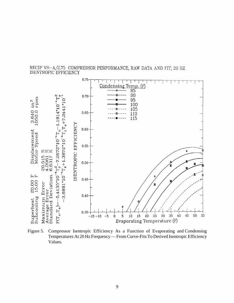
5 Compressor Isentropic Efficiency As a Function of Evaporating and Condensing Temperatures At 20 Hz Frequency — From Curve-Fits To Derived Isentropic Efficiency Values . . . . . . . . . . . . . . . 9
6 Compressor Isentropic Efficiency As a Function of Evaporating and Condensing Temperatures At 45 Hz Frequency — From Curve-Fits To Derived Isentropic Efficiency Values . . . . . . . . . . . . . . . 10
7 Compressor Isentropic Efficiency As a Function of Evaporating and Condensing Temperatures At 60 Hz Frequency — From Curve-Fits To Derived Isentropic Efficiency Values . . . . . . . . . . . . . . . 11
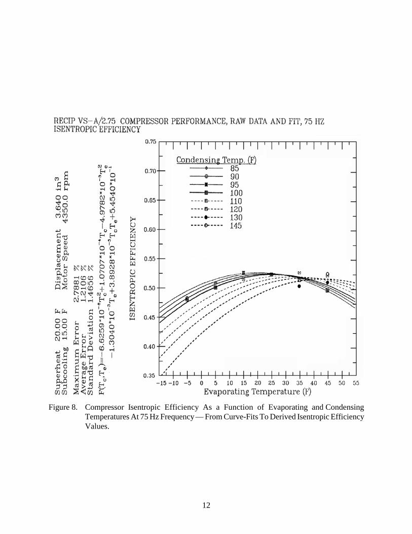
8 Compressor Isentropic Efficiency As a Function of Evaporating and Condensing Temperatures At 75 Hz Frequency — From Curve-Fits To Derived Isentropic Efficiency Values . . . . . . . . . . . . . . . 12
9 Compressor Isentropic Efficiency As a Function of Evaporating and Condensing Temperatures At 90 Hz Frequency — From Curve-Fits To Derived Isentropic Efficiency Values . . . . . . . . . . . . . . . 13
10 Modulating, Sine-Wave-Driven, Induction Motor (SWDIM) Efficiency— Reference 3-Phase, 2-Pole, 2.75 Hp Compressor Motor . . . . . . . . . . . . . . . . . 17
11 Modulating, Sine-Wave-Driven, Induction Motor (SWDIM) Slip Difference— Reference 3-Phase, 2-Pole, 2.75 Hp Compressor Motor . . . . . . . . . . . . . . . . . 18

viii
LIST OF FIGURES (continued)
Figure Page
12 Modulating Drive (Motor and Inverter) Efficiency of a Permanent-Magnet, Electronically-Commutated Motor (PM-ECM) — Reference 3-Phase, 4-Pole, 3 Hp Compressor Motor . . . . . . . . . . . . . . . . . . . 19
13 Modulating Drive (Motor and Inverter) Efficiency of a Permanent-Magnet, Electronically-Commutated Motor (PM-ECM)— Reference 3-Phase, 12-Pole, 1/5 Hp Blower Motor . . . . . . . . . . . . . . . . . . . . 25
14 Solution Logic of ORNL Modulating HPDM With Charge-Determining Option Selected . . . . . . . . . . . . . . . . . . . . . . . . . . . . . 30
15 Solution Logic of ORNL Modulating HPDM With Charge-Balancing Option Selected . . . . . . . . . . . . . . . . . . . . . . . . . . . . . . . 31
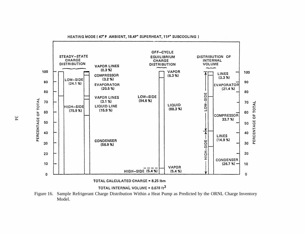
16 Sample Refrigerant Charge Distribution Within a Heat Pumpas Predicted by the ORNL Charge Inventory Model . . . . . . . . . . . . . . . . . . . . . . 34
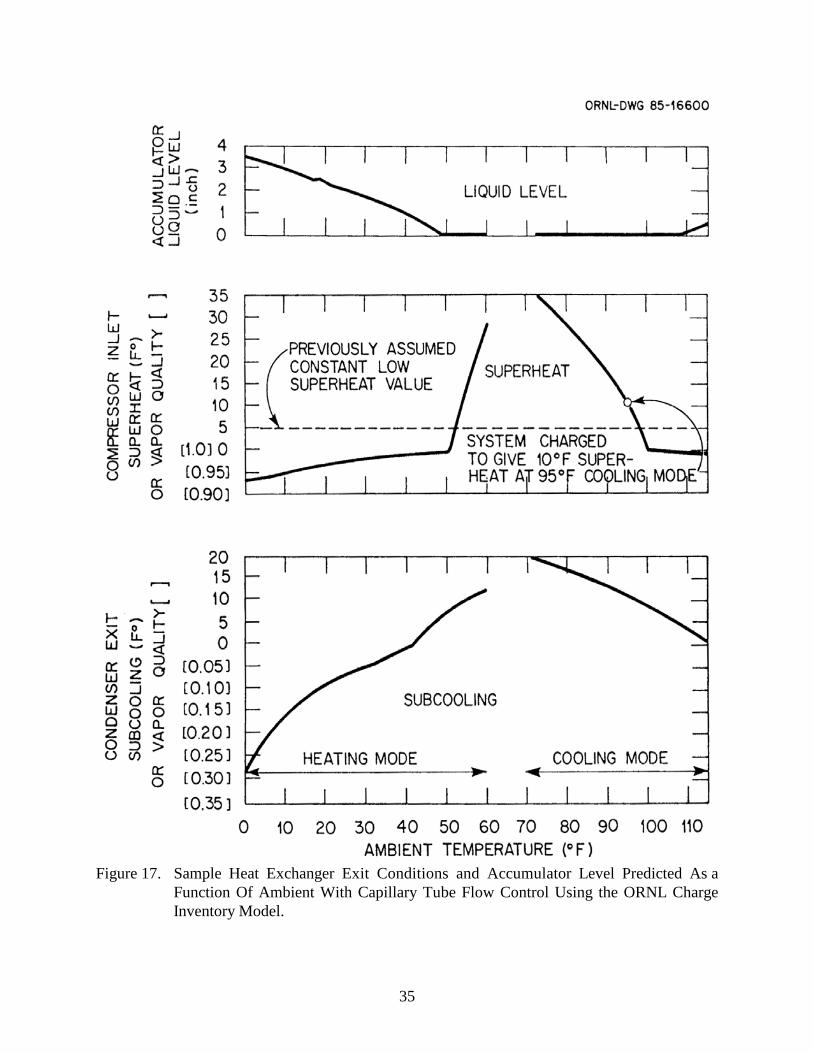
17 Sample Heat Exchanger Exit Conditions and Accumulator LevelPredicted As a Function Of Ambient With Capillary Tube Flow Control Using the ORNL Charge Inventory Model . . . . . . . . . . . . . . . . . . . . . . . . . . . . . . 35
18 Overall Structure of ORNL Modulating Contour Data Generating Program — MODCON . . . . . . . . . . . . . . . . . . . . . . . . 41
19 Detailed Structure of ORNL Modulating Heat Pump Design Model . . . . . . . . . . 42
20 Structure of Thermodynamic Supporting Routines for Refrigerant and Air Properties . . . . . . . . . . . . . . . . . . . . . . . . . . . . . . . . . . . . 43

ix
LIST OF TABLES
Table Page
1 Efficiency Degradation Multipliers For Compressor First-Generation IDIMs . . . 14
2 Efficiency Degradation Multipliers For Compressor SOA IDIMs . . . . . . . . . . . . 15
3 Reference SWDIM Efficiency For Blower Applications . . . . . . . . . . . . . . . . . . . 22
4 Efficiency Degradation Multipliers For Blower First-Generation IDIMs . . . . . . 23
5 Efficiency Degradation Multipliers For Blower State-Of-The-Art IDIMs . . . . . . 23
6 Definitions Of Charge Inventory Output Variables . . . . . . . . . . . . . . . . . . . . . . . 33
A.1 Description of CONCHZ Input Data to MODCON Program . . . . . . . . . . . . . . . . 55
A.2 Key to Independent Contour Variables Available for Selection in Input Data File CONCHZ . . . . . . . . . . . . . . . . . . . . . . . . . . . . . . . . . . . . . . . . . 59
A.3 Key to Steady-State Dependent Contour Variables Available for Selection in Input Data File CONCHZ . . . . . . . . . . . . . . . . . . . . . . 61
A.4 Key to Seasonal Dependent Contour Variables Available for Selection in Input Data File CONCHZ . . . . . . . . . . . . . . . . . . . . . . 65
A.5 Description of Output Contour Data File From MODCON . . . . . . . . . . . . . . . . . 67
B.1 Description of HPDATA Input to the MODCON Program . . . . . . . . . . . . . . . . . 77
H.1 Description of Optional CONTRL Input Data to MODCON Program . . . . . . . . 191


xi
LIST OF APPENDIX LISTINGS
Listing Page
A.1 Sample Contour Selection Data File ‘CONCHZ’ . . . . . . . . . . . . . . . . . . . . . . . . . 69
A.2 Annotated Sample Contour Selection Data File ‘CONCHZ’ . . . . . . . . . . . . . . . . 73
B.1 Sample Heat Pump Specification File ‘HPDATA’— 95�F Design Cooling Condition . . . . . . . . . . . . . . . . . . . . . . . . . . . . . . . . . . . 97
B.2 Sample Heat Pump Specification File ‘HPDATA’— 47�F Off-Design Heating Condition . . . . . . . . . . . . . . . . . . . . . . . . . . . . . . . . 99
B.3 Annotated Sample Heat Pump Specification File ‘HPDATA’— 95�F Design Cooling Condition . . . . . . . . . . . . . . . . . . . . . . . . . . . . . . . . . . . 101
C.1 Sample Single-Point Heat Pump Model Run— 95�F Design Cooling Condition — Summary Output . . . . . . . . . . . . . . . . . . . 107
C.2 Sample Single-Point Heat Pump Model Run— 47�F Off-Design Heating Condition — Summary Output . . . . . . . . . . . . . . . 119
C.3 Sample Parametric Heat Pump Model Run — Heating Mode, Compressor Frequency Vs Ambient — Abbreviated Output Listing . . . . . . . . . . 131
C.4 Sample Parametric Heat Pump Model Run — Heating Mode, Compressor Frequency Vs Ambient — Output Contour Data Generation File . . . . . . . . . . . . . . . . . . . . . . . . . . . . . . . . . . . . . . . . . . . . . . . . . . . 139
G.1 Input Format Description for MAPFIT Program . . . . . . . . . . . . . . . . . . . . . . . . . 167
G.2 Sample Input File for MAPFIT Program . . . . . . . . . . . . . . . . . . . . . . . . . . . . . . . 171
G.3 Sample Input File for MAPFIT Program — Annotated . . . . . . . . . . . . . . . . . . . . 173
G.4 Sample Output Listing for MAPFIT Program . . . . . . . . . . . . . . . . . . . . . . . . . . . 177
G.5 Output Format Description for MAPFIT Program . . . . . . . . . . . . . . . . . . . . . . . . 183
G.6 Sample Output File for MAPFIT Program . . . . . . . . . . . . . . . . . . . . . . . . . . . . . . 185
G.7 Sample Output File for MAPFIT Program — Annotated . . . . . . . . . . . . . . . . . . . 187

xii
LIST OF APPENDIX LISTINGS (continued)
Listing Page
H.1 Sample Control Data File ‘CONTRL’ —Selected Heating And Cooling Ambients With Operational-Variable Control . . . . . . . . . . . . . . . . . . . . . . . . . . . . . . . . . . . . . . . . 195
H.2 Annotated Sample Control Data File ‘CONTRL’ —Selected Heating and Cooling Ambients With Operational-Variable Control . . . . . . . . . . . . . . . . . . . . . . . . . . . . . . . . . . . . . . . . 197

1
THE ORNL MODULATING HEAT PUMP DESIGN TOOL —
MARK IV USER’S GUIDE
EXECUTIVE SUMMARY
The ORNL Modulating Heat Pump Design Tool consists of a Modulating HPDM (Heat PumpDesign Model) and a parametric-analysis (contour-data generating) front-end. Collectively theprogram is also referred to as MODCON which is in reference to the modulating and the contourdata generating capabilities. The program was developed by Oak Ridge National Laboratory for theDepartment of Energy to provide a publicly-available system design tool for variable- and single-speed heat pumps.
Overview Of New Features
MODCON predicts the steady-state heating and cooling performance of variable-speed electric-driven vapor compression air-to-air heat pumps for a wide range of system configuration andoperational variables. Engine-driven vapor-compression heat pump systems can also be modeledwith appropriate engine models supplied by the user. The present model is an extension of the(single-speed) ORNL Mark III HPDM (Fischer and Rice 1988) with the following key additionalcapabilities and improvements:
• variable-speed electric-driven compressors and/or fans with four levels of drivetechnology,
• substantially improved and extended air-side heat exchanger correlations formodulating applications,
• a refrigerant charge inventory option allowing the user to either specify or determinethe required charge,
• provision for variable-opening flow controls used in modulating heat pumps, e.g.,pulse-width-modulated (PWM) valves, stepper motors, thermal electric valves(TEV’s) and thermal expansion valves (TXV’s),
• provision for input selection of refrigerant and the addition of R134a to therefrigerant choices, and
• automated means to conduct parametric performance mappings of selected pairs ofindependent design variables.

2
The user can generate steady-state performance data sets at fixed ambients or as a function ofambient temperature. The range of selection options includes:
• 52 design and control variables for parametric analysis,
• 8 user-defined operational control relationships as functions of compressor speed orambient temperature, and
• over 100 possible heat pump model output parameters.
Basic modulating compressor performance is represented by the use of performance maps at discretespeeds with interpolations and extrapolations as necessary to represent a continuous range of speedcontrol. Continuously-variable-speed operation of both induction-motor and electronically-commutated-motor (ECM) types are modeled. Compressor motor performance of both types can besimulated based on a specified motor size or, alternatively, each motor can be sized automaticallyby the model to operate at a required percentage of rated load.
For modulating blowers and fans, required modulated power can be computed from first principlesor referenced to a specified nominal power at design speed. For ECM blowers and fans, a full rangeof motor sizing options is also available.
The combination of the above capabilities provides a general tool for system configuration designand operational control of variable-speed heat pumps. The tool can be used to automate thegeneration of extensive simulation datasets for design studies. These datasets, once generated, canbe accessed independently by other engineers to plot and analyze selected dependent performancevariables of interest in two- or three-dimensional space. The program execution time is sufficientlyfast so that a parametric evaluation in two variables can be performed in less than 30 seconds on aPentium III, 300 MHZ PC. An example of the use of the model for a complete design analysis of aECM-driven variable-speed system is given by Rice (1992).
Validations and Applications
Modulating model validations were conducted on an initial version of the ORNL Modulating HPDMusing measurements on a modified commercially-available variable-speed heat pump tested atORNL. The model was compared to experimental trends with respect to compressor and indoorblower speeds and also the basis of absolute COPs and capacities. The trends in COP and capacitywere generally well predicted as reported by Miller (1988a).
The results of the absolute comparisons over a range of speeds and ambients indicated that bestmodel agreement was obtained at the lower speeds in both heating and cooling mode, with increasingperformance overpredictions (to maximums of about 10% in both COP and capacity) occurring athigher speeds. This increase in model overprediction with speed occurs because of limitations of thesimplified models of refrigerant circuitry with the higher subcooled (and/or superheated), moreheavily loaded heat exchanger conditions.

3
Different versions of the single-speed model have been validated by various researchers for bothsingle-speed and dual-stroke heat pumps. The single-speed model has also been used by others inthe simulation of variable-speed engine-driven heat pumps (Fischer 1986b, Monahan 1986, and Rusk1990). With one exception, the validations of the original single-speed version in bothnonmodulating and modulating applications of sizes from 2 to 10 tons capacity have been reportedas satisfactory to excellent.
The electric-driven version has been used as 1) an aid in the experimental evaluation of optimalhardware control, 2) as a tool to determine potential performance levels for residential unitaryequipment, and 3) as a tool to assess the potential of variable-speed drives for commercial unitaryequipment.
The program has also been modified to be used with newer HFC refrigerant alternatives such asR134a. With this capability, the ORNL Modulating Heat Pump Design Tool is ready to be utilizedfor the equipment redesign issues facing heat pump manufacturers in the coming decade.
VARIABLE-SPEED COMPRESSORS
Basic Compressor Representation
Manufacturers’ compressor performance maps based on calorimeter tests are the starting point forthe modulating compressor model. These maps at a given drive frequency are functions ofcompressor inlet and exit conditions — typically defined by evaporating and condensing saturationtemperatures and suction superheat. The map-based option for compressor representation is the onlychoice developed for the modulating model (the other possible choice being the loss-and-efficiencymodel discussed previously in the ORNL report by Fischer and Rice 1983). Positive displacementcompressors of reciprocating, rotary, and scroll type for which manufacturers’ map data are availablecan be modeled. Single-speed, multiple-speed, and continuously-variable-speed compressors can beaccommodated if the appropriate performance maps are available.
With some adjustments, both low and high-side-cooled compressors with varying amounts of suctionsuperheat can be handled. As in earlier versions of the ORNL HPDM, the default suction gassuperheat corrections are somewhat specific to reciprocating compressors but can be generalized bysuitable adjustment of superheat correction factors set in BLOCK DATA. These corrections as wellas newer adjustments for motor efficiency effects on suction gas superheat assume low-side motorcooling as the default. However, this assumption can also be changed by suitable adjustment ofBLOCK DATA parameters.
Modulating Compressor Performance
Compressor performance as a function of speed is represented by the use of maps at discretefrequencies with interpolations and extrapolations as necessary to represent a continuous range ofspeed control. The modulating HPDM requires the user to input compressor map-based coefficientsfor power and mass flow rate (or alternatively, for derived isentropic and volumetric efficiency based

4
on compressor shell conditions) as functions of operating conditions at each speed for whichsufficient data are available.
In cases where minimal data are available, curve fits to the derived efficiency values have been foundto often give more reliable interpolations and extrapolations over speed than similar representationsbased on basic power and mass flow data. All the curve fit representations are biquadratic functionsof condenser and evaporator saturation temperatures except for volumetric efficiency. Because ofthis, all extrapolations of polynomial curve fits are inherently suspect and should be tested foracceptable behavior outside of the fitting data range. The latter is a linear function of pressure ratioand a quadratic function of discharge pressure. The specific forms of the curve-fitting equations aregiven in Table B.1 describing the required heat pump specification file. Further description of thepower and mass flow rate equations can be found in the ORNL report by Fischer and Rice (1983).
The interpolations in power and refrigerant mass flow rate (or in isentropic and volumetricefficiency) are presently done linearly with frequency. This can be rather easily changed to quadraticif desired by changing the value of NPT from 2 to 3 in the CMPMAP subroutine. Extrapolations,if necessary, are always done linearly.
Compressor Map-Fitting Program
A compressor-map-fitting program is provided with the HPDM to fit compressor manufacturers’available map data into either of the above representations. Appendix G describes the input data andformat requirements for the curve-fit program. Sample plots of curve fits by the two methods tocompressor data of a specified frequency of 30 Hz are shown in Figures 1 – 4. In Figures 5 – 9, curvefits to isentropic efficiency at other frequencies (20, 45, 60, 75, and 90 Hz) are shown. All plots arefor a reference sine-wave-driven, induction motor (SWDIM) compressor calorimeter-tested at ORNLby Miller (1989) and supplemented by data provided by the manufacturer. The curve-fit coefficientsfor this compressor are included in the sample data sets of Appendix B.
The map-fitting program also prints tabular results comparing the individual data points to theircorresponding curve fit values. Additional tables are generated for the direct power and mass flowrate curve-fits showing the differences between the resultant isentropic and volumetric efficienciesversus the values derived directly from the map data. With this information, the user can judge whichcurve-fitting approach is more suitable for their data.
The map-fitting program can be run for any number of speeds and will create a data file of curve-fitcoefficients of the format required by the heat pump specification file. This file can be imported intoan existing heat pump data file with only minor editing required. The program can also convert themaps to superheat or return gas temperature conditions other than those for which compressor mapdata are available.

5
Figure 1. Compressor Isentropic Efficiency As a Function of Evaporating and CondensingTemperatures At 30 Hz Frequency — From Curve-Fits To Basic Power and RefrigerantMass Flow Rate Data.

6
Figure 2. Compressor Volumetric Efficiency As a Function of Pressure Ratio and CondensingPressure At 30 Hz Frequency — From Curve-Fits To Basic Power and Refrigerant MassFlow Rate Data.

7
Figure 3. Compressor Isentropic Efficiency As a Function of Evaporating and CondensingTemperatures At 30 Hz Frequency — From Curve-Fits To Derived Isentropic EfficiencyValues.

8
Figure 4. Compressor Volumetric Efficiency As a Function of Pressure Ratio and CondensingPressure At 30 Hz Frequency — From Curve-Fits To Derived Volumetric EfficiencyValues.
9
Figure 5. Compressor Isentropic Efficiency As a Function of Evaporating and CondensingTemperatures At 20 Hz Frequency — From Curve-Fits To Derived Isentropic EfficiencyValues.

10
Figure 6. Compressor Isentropic Efficiency As a Function of Evaporating and CondensingTemperatures At 45 Hz Frequency — From Curve-Fits To Derived Isentropic EfficiencyValues.

11
Figure 7. Compressor Isentropic Efficiency As a Function of Evaporating and CondensingTemperatures At 60 Hz Frequency — From Curve-Fits To Derived Isentropic EfficiencyValues.
12
Figure 8. Compressor Isentropic Efficiency As a Function of Evaporating and CondensingTemperatures At 75 Hz Frequency — From Curve-Fits To Derived Isentropic EfficiencyValues.

13
Figure 9. Compressor Isentropic Efficiency As a Function of Evaporating and CondensingTemperatures At 90 Hz Frequency — From Curve-Fits To Derived Isentropic EfficiencyValues.

14
Modulating Drive Options
Drive Efficiency Options. Four drive efficiency conversion options are available in the program.They are:
1) a moderate-efficiency inverter drive (first-generation IDIM),
2) a high-efficiency inverter drive (state-of-the-art IDIM),
3) an ideal sine-wave-driven induction motor (SWDIM) [limiting case for modulating inductionmotor],
4) an electronically commutated motor (ECM) The user-supplied compressor data can be for an inverter-driven system (either IDIM or ECM) orfor a reference SWDIM compressor. The user selects whether this base compressor map is to remainunmodified or be converted to one of the above drive types.
If a conversion is to be made, the user must be especially careful to properly identify the suppliedmap with one of the four types so that the most accurate conversion is made. The potential errorinvolved in such conversions is reduced if the base map data is for a SWDIM drive. This is typicallyobtained by testing the compressor with a variable-frequency motor-generator set. The SWDIMoption is also useful in evaluating the total system loss resulting from the direct (inverter) andindirect (increased motor inefficiency and suction gas superheat) losses of inverter-driven inductionmotors.
IDIM Correction Factors. Efficiency reduction factors for first-generation IDIMs were based oncomparative 2.75-ton hermetic reciprocating compressor tests using alternately a voltage-source-inverter (VSI) and a motor-generator (m-g) set (the SWDIM reference) as described by Miller(1988b). From these tests conducted at representative modulating conditions, the followingefficiency multipliers of Table 1 were determined for the combined motor and inverter efficiencyof first-generation IDIMs relative to SWDIM efficiency:
Table 1. Efficiency Degradation Multipliers ForCompressor First-Generation IDIMs
Drive Frequency Heating Mode Cooling Mode
15 0.621 0.62530 0.784 0.80945 0.840 0.86060 0.868 0.84175 0.878 0.83 (est.)90 0.879 0.82 (est.)

15
By the nature of the tests, these factors include any suction gas heating differences between the twodrive types.
Similar multipliers were developed for the state-of-the-art IDIM option using bench efficiency dataon high-efficiency VSI inverter drives and model simulations of the corresponding referenceSWDIM efficiency — both obtained from Lloyd (1987). The efficiency degradation multipliersobtained from this information in shown in Table 2.
Table 2. Efficiency Degradation Multipliers ForCompressor SOA IDIMs
Drive Frequency Heating Mode Cooling Mode
15 0.82 (est.) 0.78 (est.)30 0.87 0.87245 0.908 0.91560 0.921 0.91975 0.929 0.920 (est.)90 0.946 0.920 (est.)
By the nature of this data, these factors do not include any suction gas heating differences betweenthe two drive types — although as these degradation factors are closer to unity, this secondary effectwould be expected to be small. In all the above cases, the motors were 2-pole with nominal speedsof 3450 – 3500 rpm.
Induction-Motor (IM) to ECM Conversion. The user can have the program simulate thereplacement of the drive used in an IDIM or SWDIM compressor drive with a PM-ECM drive. Thisreplacement option will allow the same basic modulating compressor characteristics to be appliedwith a different drive characteristic. In this way, calorimeter data with existing compressors anddrives can be used with more advanced drive combinations.
Most compressor maps are available only for induction-motor (IM) drives. Many of these are forsingle-speed motors (equivalent to the SWDIM option but only for one or at most two frequencies,i.e., 50 and 60 Hz). The variable-speed compressor data are usually for IDIMs of either the PWMor VSI type. Variable-speed SWDIM data are rather scarce. However, as this latter type of data hasfewer uncertainties with regard to the level of inverter-waveform-related losses, it is preferred forcases where a conversion of motor type is required.
To make such a conversion, it was necessary to provide to the model representative SWDIM andECM performance at least as a function of drive frequency. However, to avoid having to preselectan appropriate torque vs speed profile for the drives and to further provide for motor sizinggenerality, complete mappings of representative SWDIM and ECM performance as a function ofnormalized drive frequency and torque were incorporated.

16
SWDIM Performance. Performance information on a representative sine-wave-driven inductionmotor were obtained from Zigler (1987). He generated simulated sine-wave performance maps onan existing variable-speed motor for which the basic motor characteristics were well known and forwhich standard motor efficiency test data were available at the standard motor rating temperatureof 77�F (25�C).
From these empirical simulations, motor efficiency and slip were provided for a 2.75 hp (2.05 kW),2-pole, 3-phase motor over a range of frequencies from 15 to 90 Hz, a range of torques from 20 to200% of nominal, and a range of voltages from 90% to 110% of nominal. Nominal torque was at60 Hz frequency (3450 rpm). All simulated values were for estimated typical rotor and statortemperatures in a hermetic compressor environment. Motor windage and friction losses were notincluded in the motor efficiency values. Contour plots of the SWDIM performance mappings formotor efficiency and slip are shown in Figures 10 and 11.
To provide further analysis flexibility, the motor data were generalized in the model to apply to anormalized speed range of 25 to 150% of nominal and for motor sizes other than the original 2.75 hp(2.05 kW). However, the original basis for the data are provided here so that users can make theirown judgements as to whether or not such generalizations are sufficiently accurate for their specificanalysis purposes.
The SWDIM motor for which data were provided was, in fact, the same model motor used in thereference SWDIM compressor tested by Miller (1989). Therefore, when used together, these twodata sets provide a most consistent basis for extraction of the SWDIM performance and replacementwith ECM efficiency characteristics.
ECM Performance. Dynamometer performance data were obtained from Young (1990) on a pro-duction 4-pole, 3 hp (2.24 kW) ECM for a range of compressor speed and torque. As there is nomotor slip in an ECM motor, speed is directly proportional to drive frequency. Therefore, for ECMs,only motor efficiency as a function of speed and torque is needed to characterize motor performance.
The range of motor speed was from 1000 to 6250 rpm with a nominal speed of 5400 for anormalized speed range of 0.2 to 1.15 of nominal. The torque range was from about 20 to 190% ofthe nominal value. No windage and friction losses were included as for the SWDIM case; however,estimated magnetization losses due to the permanent magnet rotor were included.
Similarly as for the SWDIM motor data, the ECM performance data were generalized to apply fornominal speeds and motor sizes other than that for which the data were available. Contours ofcompressor ECM drive efficiency as a function of speed and fractional load are shown in Figure 12.
ECM Operating Temperature Corrections. The ECM data were taken at the standard motor ratingtemperature of 77�F (25�C). Therefore, to properly apply the data to a hermetic application,correction factors for motor temperature effects were developed. These were based on informationprovided by Zigler (1987) and supplemented by Young (1990) and are functions of stator and rotortemperature, winding resistances, the motor current vs torque relationship, and magnet fluxtemperature coefficients. Appropriate values for these parameters are specified in BLOCK DATA

17
Figure 10. Modulating, Sine-Wave-Driven, Induction Motor (SWDIM) Efficiency — Reference 3-Phase, 2-Pole, 2.75 HpCompressor Motor.

18
Figure 11. Modulating, Sine-Wave-Driven, Induction Motor (SWDIM) Slip Difference — Reference 3-Phase, 2-Pole,2.75 Hp Compressor Motor.

19
Figure 12. Modulating Drive (Motor and Inverter) Efficiency of a Permanent-Magnet, Electronically-Commutated Motor(PM-ECM) — Reference 3-Phase, 4-Pole, 3 Hp Compressor Motor.

20
for two nominal-speed designs; the corrections for other nominal speeds are determined byinterpolation.
IM-To-ECM Conversion Procedure. For given compressor operating conditions and operatingfrequency, the model first calculates the compressor input power for the base compressor map. Givenfrequency and drive input power, the motor operating speed, torque and efficiency can be found byiteration using the reference SWDIM performance maps (and the efficiency corrections for directand indirect inverter losses, depending on the type of compressor drive). The computed torque andthe specified frequency are next used with the ECM performance map to calculate the efficiency ofthe replacement motor. This difference in efficiency is then applied to the power requirementspredicted from the baseline compressor map. Corrections for the differences in speed between theSWDIM and the ECM operating at the same frequency are also applied to the power and refrigerantmass flow rate values.
Secondary Effects of Reduced Suction Gas Superheating. An approximate method was alsodeveloped to adjust for the performance effects of reduced suction gas superheating with the moreefficient ECM motor. The reduction in motor losses resulting from the use of a more efficient motoris calculated and an estimated portion of this is used to reduce suction gas heating from a computedbaseline level. The effect of this estimated superheat reduction on ideal compression work is appliedas a secondary correction ratio to the overall isentropic efficiency. The result is an approximatemeasure of the compounded benefit of conversion to the more efficient ECM drive.
Motor Sizing/Loading Options
Compressor motor performance of either IDIM, SWDIM, and ECM types can be simulated basedon a specified motor size or, alternatively, each motor can be sized automatically by the model tooperate at a required percentage of rated load.
Automatic Motor Sizing. In this option, users can investigate alternative motor sizing choices bydirectly selecting the degree of loading (percent of rated torque) at which they would like the motorto operate on the appropriate motor efficiency curve . This percentage is then specified in place ofmotor size and the model will determine the required size to maintain motor operation at thisloading.
This approach is advantageous when users know where they would like the motor to operate on itsperformance curve (i.e., the specific motor sizing strategies they would like to evaluate) and wouldlike to maintain that point (and efficiency) while various system configurations and/or operatingvariables (such as air flow rates) are being evaluated. Then once the system configuration is decidedupon, the program determines the required motor size.
Specified Motor Size. This option is most useful once the motor size has been fixed by a previousdesign analysis or when only certain sizes are available for consideration. The user directly specifiesthe desired motor size (in hp) for the selected drive type. The model uses the chosen size along withthe selected nominal speed to compute a nominal torque. This rated torque is then compared to therequired operating torque to determine the resultant fractional loading on the motor. The motor

21
performance curves are then used to determine the motor efficiency and speed (for IMs) at theoperating torque and drive frequency ratios.
In this approach, the motor efficiency at a given speed will change as the system configuration andoperating conditions change. Specified motor sizes are the preferred approach at off-designconditions during the design process and at all operating conditions once the system design has beenfinalized. It should be noted that if a compressor base displacement is scaled manually by the user,the specified motor size should be scaled similarly.
A recommended procedure for sizing compressor motors and simulating off-design performance fora modulating application using these options has been presented by Rice (1992).
VARIABLE-SPEED BLOWERS
Modulating Blower Performance
Modeling Perspective Relative To That For The Compressor. The modeling of variable-speeddrives for blowers and fans is somewhat more straightforward than for compressors. This is becausea combined blower(or fan)/motor/drive performance map is not required to be provided by the useras in the case of the compressor. Blower/fan performance is instead handled separately from that ofthe motor/drive combination.
Whereas compressor efficiency (both isentropic and volumetric) varies with speed, to a closeapproximation, blower and fan efficiencies remain constant with speed (from the fan laws).Therefore the modeling assumptions and options provided for modeling blower and fan efficienciesdiscussed by Fischer and Rice (1983) hold equally well for modulating air flows.
The primary added capability in the new model which relates to blower- and fan-only efficienciesis the new option of being able to specify a nominal power from an existing system and have theprogram internally compute and apply the implicit impeller efficiency (based on the calculated air-side pressure drop) to a new drive type.
General Capabilities. For modulating blowers and fans, the required fan power can be computedfrom first principles or referenced to a specified nominal power at design speed. The conversion-option categories available for modulating blowers and fans is similar in type to that provided forthe compressor drives — first generation and SOA IDIM, SWDIM, and ECM. For all drive types,the program will compute the required motor size (when the model is run at nominal speed).However, only for ECM blowers and fans is the full range of motor sizing options available —comparable to that provided for all drive types in the case of compressors.
The blower/fan drive models are based on:
• first-generation IDIM and SWDIM blower drive efficiency data derived from ORNLtests of a modulating heat pump conducted by Miller (1988b), and

22
• SOA IDIM versus SWDIM comparative efficiency data obtained from a motormanufacturer (Lloyd 1987),
Reference SWDIM. The reference SWDIM data built into the model was taken from combinedblower and motor tests of Miller (1988b) on a three-phase, six-pole, 1/3 hp (0.25 kW) air handler.A variable-frequency motor-generator was used for the baseline test and the volts/Hz ratio of themotor was adjusted at each tested frequency to maintain best efficiency.
A nominal efficiency of 75% was obtained from the motor manufacturer and used to determine ablower-only efficiency of 28% at nominal speed. By assuming the blower efficiency was constantwith speed, motor efficiencies were derived from measured blower power for the range of testedfrequencies from 25 Hz to 60 Hz. As the tests were performed in an actual air handler unit, theappropriate fan load for a modulating application was automatically provided.
The resultant reference SWDIM efficiencies taken from a curve-fit and extrapolation (where shownas estimated) of the derived efficiency points are tabulated in Table 3 as a function of drivefrequency. The function FANSWV contains a curve-fit representation of these data points.
Table 3. Reference SWDIM EfficiencyFor Blower Applications
Drive Frequency SWDIM Efficiency
15 0.40 (est.)20 0.52 (est.)25 0.58430 0.63735 0.68040 0.71245 0.73250 0.74555 0.75060 0.750
First-Generation IDIM. The same procedure was used to derive drive efficiencies from similar air-handler tests over a slightly wider speed range conducted by Miller (1988b) on the same motor witha first-generation VSI inverter drive. The derived IDIM efficiencies were divided by theircorresponding SWDIM values to obtain efficiency degradation factors due to the direct and indirectinverter losses (Miller 1988b). These multipliers are given in Table 4 — a curve fit of which is builtinto the model in function FANFGN.

23
Table 4. Efficiency Degradation MultipliersFor Blower First-Generation IDIMs
Drive Frequency Multiplier
15 0.13 (est.)20 0.23 (est.)25 0.3630 0.4735 0.5640 0.6245 0.6950 0.7555 0.8060 0.82
SOA IDIM. For state-of-the-art (SOA) IDIMs, bench test efficiency data taken under representativefan loading conditions were obtained from a motor manufacturer (Lloyd 1987). The correspondingSWDIM performance at the same conditions was also estimated by the manufacturer. From thesedata, consistent degradation factors for the SOA IDIMs were obtained. The resultant degradationfactors for SOA IDIMs are shown in Table 5 — a curve-fit representation of which is contained infunction FANSOA.
Table 5. Efficiency Degradation MultipliersFor Blower State-Of-The-Art IDIMs
Drive Frequency Multiplier
15 0.32 (est.)20 0.45 (est.)25 0.5830 0.6635 0.7340 0.7845 0.8350 0.8655 0.8960 0.92
ECM Indoor Blower and Outdoor Fan Performance. For both the indoor blower and outdoor fanmodulating drives, an efficiency map obtained from Young (1990) for a 12-pole, 1/5 hp (0.15 kW)production ECM as a function of speed and torque was used. The range of motor speed was from300 to 1300 rpm with a nominal speed of 1200 for a normalized speed range of 0.2 to 1.15 ofnominal. The torque range was from about 20 to 160% of the nominal value. Windage and friction

24
losses were included as were magnetization losses due to the permanent magnet rotor. A plot of theblower ECM performance mapping is shown in Figure 13.
The torque range for the 1/5 hp ECM was generalized in the model to be applicable for othernominal motor sizes as specified by the user. The ECM speed range was not normalized, however,as it was felt that it would be less likely to have a range of fan motors designed for different nominalspeeds available (in contrast to the compressor where a redesigned motor would have more potentialfor energy savings). By not normalizing the blower ECM speed range, it was also possible to moreeasily simulate the more common use of different speed taps on a single ECM drive to meet differentapplication requirements with the same nominal speed design. In this way, the same basic drivedesign can be applied to indoor blowers and outdoor fans with different nominal speeds (e.g.1080 rpm for the blower and 825 rpm for the outdoor fan).
Further Discussion of Blower and Fan Modeling Capabilities
Model Calibration Options. As noted earlier, there are two options for computing modulatingblower or fan power — by first principles or based on a baseline nominal power input. For aspecified operating frequency and drive type, the first principles approach uses model-calculated airflow, pressure drops, and blower and blower drive efficiencies to directly calculate required fanpower based on the given indoor or outdoor unit air-side configuration. If the computed values donot agree closely enough with available test data, the input values of blower efficiency and/or thecoil/system pressure drop multipliers can be adjusted at one test condition in each mode (to accountfor wet-to-dry coil effects) to calibrate the model.
An alternative approach which can be more convenient when comparing to existing hardware is tospecify known nominal power values for the indoor and/or outdoor units and the associated drivetypes. The model will compute the proper modulating fan power based on the fan laws and the ratioof drive efficiencies between the baseline and the selected drive types at the specified operatingfrequency. In this alternative approach, the calculated system pressure drop is not used directly inthe fan power calculations but is used to compute the implied blower efficiency and the requiredmotor size.
Indoor Duct System Options. The options for specifying the indoor duct system have been enhancedto provide more convenient ways to control the external pressure drop seen by the indoor blower fornominal design conditions. In place of a specified duct size, a fixed external pressure drop can nowbe specified to meet ARI minimum requirements (ARI 1989) or to agree with a measured value fora given test setup. The required duct size is also computed in this case so that this value can, in turn,be specified for an off-design-point calculation (Rice 1992).
Coil and indoor system (which includes the built-in heater and filter correlations) pressure dropmultipliers have been added to the input to provide further model calibration capability.
ECM Motor Sizing Options. For the blower and fan motors, speed versus torque maps are suppliedonly for the ECM drives. As a result, motor size or loading selections are possible only for theECMs. Otherwise, these options work the same as for the compressor case. A recommended

25
Figure 13. Modulating Drive (Motor and Inverter) Efficiency of a Permanent-Magnet, Electronically-Commutated Motor(PM-ECM) — Reference 3-Phase, 12-Pole, 1/5 Hp Blower Motor.

26
approach to sizing ECM blower and fan motors and simulating off-design performance for amodulating application using these options has been presented by Rice (1992).
AIR-SIDE CORRELATIONS FOR MODULATION AND ENHANCED SURFACES
Advantages and Features
A major update of air-side heat transfer and pressure drop calculations was completed for improvedprediction for modulating air flows based on work by Gray and Webb (1986). Other heat exchangermodeling improvements included the addition of augmentation treatments of wavy and louveredsurfaces dependent on Reynolds number and fin pattern specifics. The calculation of coil entranceand exit losses is now done explicitly rather than as just a percentage of the calculated loss.
The benefits of these changes are:
• improved low flow correlations over those used in the ORNL Mark III Model,
• added flow and geometry -dependent augmented surface analysis, and
• more consistent treatment of ancillary air-side pressure losses
New Baseline Air-Side Correlations. The baseline air-side heat transfer and pressure dropcorrelations (McQuiston 1981) used in the ORNL Mark III HPDM (Fischer and Rice 1983) werereplaced by more accurate representations by Gray and Webb (1986). These newer correlationsdeveloped for plain fin-and-tube heat exchangers are especially improved at low Reynolds numbersand for prediction of the row effect. This is primarily because Gray and Webb made corrections forexperimental error in the original data taken by earlier researchers which had been used byMcQuiston. Furthermore, the correlations are much better behaved at low flow rates, as areextrapolations beyond the available test range — which are sometimes needed with modulatingapplications when exploring the design envelope.
Correction Factor Format. The Gray and Webb smooth-fin correlations were used as the newreference base for plain, wavy, and louvered fin options in the ORNL Modulating HPDM. Allaugmented surface correlations were represented as correction factors (multipliers), of varyingdegrees of complexity, to the reference smooth fin equations. This is an especially useful format asmost reported data on improved surfaces are for a limited number of tube size, spacing, and rowconfigurations. The referencing of all the correlations to the general model for plain fins adds bothgenerality and consistency to the correlation predictions.
New Geometry and Flow-Dependent Correction Factors. The wavy- and louvered-fin enhancementchoices are now offered at two levels of complexity. The first level is as was done in the Mark IIIModel where constant multipliers are applied to the (new) baseline plain-fin equations. The secondlevel choices are to use multiplier correlations which are now dependent on Reynolds number andfin pattern specifics. For wavy (zig-zag) fins, correlations developed for ORNL by Beecher andFagan of Westinghouse R & D Center (1987) were used. For simple louvered fin patterns, the

27
multiplier correlations obtained from Makayama and Xu (1983) were used. These second-leveloptions require additional user input to specify the details of the fin patternations.
Further Improvements In Pressure Drop Calculations. The air-side pressure-drop correlations werefurther revised, beyond the change to newer reference plain-fin correlations, to improve theconsistency of the calculations for the various options. Explicit calculations were added of entranceand exit pressure losses and velocity head loss using expansion and contraction coefficients andmethodology from Kays and London (1974). User-supplied pressure-drop adjustment factors werealso added for optional application to the overall coil pressure drops and the indoor system pressuredrop.
CHARGE INVENTORYAND RELATED WIDE-RANGE FLOW CONTROL OPTIONS
Advantages and Features
Overview. A summary of the advantages of the charge inventory capability are as follows:
• Allows the user to either specify or determine refrigerant charge,
• Enables more realistic off-design predictions for a rangeof flow control types, and
• Accommodates variable-opening flow control devicesneeded for modulating heat pumps— e.g., PWM valve, stepper motor, TEV’s and TXV’s.
A major new feature of the ORNL Modulating HPDM is refrigerant charge (mass) inventorycapability. This capability can be used in the HPDM in two ways. The user can either specify ordetermine the refrigerant charge requirements. In the first option, the user specifies the refrigerantcharge and requires the model to adjust the operating conditions so that the system requires exactlythat amount of active charge (charge balancing). The latter approach is to specify desired operatingconditions and have the model calculate the required charge to obtain those conditions (chargedetermining).
The charge-balancing procedure is more useful in simulating system performance withpredetermined flow control hardware over a range of off-design operating conditions. The charge-determining alternative is useful in evaluating system charge and storage requirements in the designphase when the equipment is being evaluated for (or being controlled to obtain) optimum condensersubcooling or flow control sizing and evaporator superheat levels over a range of operatingconditions.
The charge inventory feature can also be turned off completely. In this case, the model calculationsare essentially the same as for the Mark III version.

28
Charge-Balancing Option. With a charge inventory balance, one can predict the effects of a givencharge level on systems with little or no charge storage capacity or predict the levels at which over-or under-charging effects begin to occur. The additional information about system charge-balancingrequirements enables more realistic off-design predictions for a range of flow control approaches.Existing and advanced (or idealized) variable-opening flow control devices, which are morenecessary in modulating systems, can be modeled more directly with the addition of a charge balance(which determines required condenser subcooling or evaporator superheat levels).
From a computational perspective, use of a charge balance requires an additional outermost iterativeloop in the heat pump solution scheme. As such, the model run-time is increased approximately bythe number of times the outermost loop must be repeated to obtain agreement between the specifiedand the calculated refrigerant charge. On each successive iteration, the evaporator exit superheat orthe condenser exit subcooling is adjusted (depending on the flow control type specified) so as tobring the calculated and specified charges into agreement.
Charge-Determining Option. In contrast, the charge-determining alternative has much lesscomputational overhead — at most a factor of about two. This option provides the designer withfeedback on how various heat exchanger size and control options affect the charge requirements butwithout prematurely limiting the range of possible system operating conditions with an additionalcharge constraint. Both the added flexibility and computational speed of the charge-determiningapproach make it a more suitable choice for initial scoping and more general system designoptimization studies.
Recommended Design Procedure. Once the optimum control conditions of the system areestablished, over a range of operating conditions without the constraints of charge inventory-balancing, the charge and flow control requirements of the idealized design can be evaluated andapproaches prescribed to approximate this in hardware. (Valve sizing information for various typesis provided in the model output.) At this stage, the charge-balancing model can be brought intoeffective use to evaluate the refrigerant charge levels needed for various flow-control types andsizings to most closely approach the thermodynamically-optimum design over the range of requiredoperating conditions. In this way, the available charge inventory options can be used in combinationto find a design which is not only workable but which also obtains the best performance out of theavailable hardware.
Flow diagrams of the HPDM solution logic for the charge-determining and the charge-balancingoptions are shown in Figures 14 and 15. The various options of specified flow control or heatexchanger exit conditions with and without a specified charge are discussed at some length in thesections to follow.
Inventory Calculation Features. The charge inventory calculational model includes the followingfeatures :
• user choice of inventory method ranging from simplified to SOA (Rice 1987). Thesimplified analytical formulation is provided for first-level analysis as it is muchfaster than the other more accurate methods that are included but which requirenumerical integration (Rice 1987),

29
• tabulations of the steady-state on- and off-cycle charge distributions in a heat pump,and
• a j-tube accumulator model adapted from the NIST mixed — refrigerant heat pumpsimulation (Domanski, 1985, 1986).
More specifics of the inventory choices and the accumulator model requirements can be found in thedescription of the HPDATA input file in Appendix B. Details of the available inventory methods,covering the different possible void fraction models and heat flux assumptions can be found in thepaper by Rice (1987). Recent heat pump validation tests with the different methods have beenreported by Damasceno et al (1991).
Modeling Interrelationships Between Refrigerant Charge and System Flow Control
As discussed in the preceding section, the inclusion of charge inventory capability in the ORNLModulating HPDM allows the user to either determine or specify the refrigerant charge inventory.The various options for specifying flow control devices or heat exchanger exit conditions with andwithout a specified charge are discussed in this section with reference to the flow diagrams shownin Figures 14 and 15. The charge-determining path is taken when refrigerant charge is not specifiedwhile the charge-balancing route is taken if a refrigerant charge level is provided.
If the refrigerant charge is not specified, the user must define, as input, values for
1) compressor inlet superheatand
2) either condenser exit subcooling directly or specific flow control devices(indirectly determining condenser subcooling).
If the refrigerant charge is specified, the user may only specify one of the above categories with theremaining category to be determined by a system charge balance. Otherwise, the system would beoverspecified. From a thermodynamic cycle perspective, either compressor inlet superheat orcondenser exit subcooling must be left as a free parameter to be determined by charge balancingwhen the refrigerant charge is an additional given quantity. If the compressor inlet superheat isspecified, the cycle is considered low-side-determined while if condenser exit subcooling (or a flowcontrol device) is specified the cycle is high-side-determined.
These choices are made in the HPDATA input data file (Appendix B) on Lines #4 and #5 where theCharge Inventory / Superheat Data and the Charge Inventory Calculational Data are specified.Related specification of condenser subcooling or specific flow control devices is made by the userunder Flow Control Device Data on Line #6.

30
Figure 14. Solution Logic of ORNL Modulating HPDM With Charge-Determining OptionSelected.

31
Figure 15. Solution Logic of ORNL Modulating HPDM With Charge-Balancing Option Selected.

32
If the refrigerant charge is to be determined,then ICHRGE is set to 0 on Line #4and IMASS is set to 1 on Line #5.
If the refrigerant charge is specified on Line #4 as REFCHG),then ICHRGE is set to 1 or 2 on Line #4 and either compressor inlet superheat
or condenser exit subcoolingis determined, respectively.
The refrigerant charge inventory values which are calculated for each system component andtabulated in the program output are given in Table 6. Listings C.1 and C.2 contain examples ofcomputed charge inventory values as listed in Table 6. Figures 16 and 17 provide some sampleresults using the charge inventory model for a heat pump system with capillary tubes and a suctionline accumulator.
If no refrigerant charge calculations are desired,then ICHRGE must be set to 0 on Line #4and IMASS is also set to 0 on Line #5.
In this latter case, the program runs as fast as the ORNL Mark III single-speed model and no charge-related output is provided.
Discussion of TXV Modeling With And Without A Charge Inventory Balance
Potential Area Of Confusion. A potential point of confusion in both the single- and variable-speedORNL heat pump models is the modeling of systems with thermal expansion valves (TXV’s). Suchvalves are often described as maintaining the compressor inlet superheat at a constant value. Becauseof this generalization, users of the single-speed model (without a charge inventory balance) oftenspecify a TXV valve and a constant compressor inlet superheat value and expect the model toproperly represent behavior of such a system over a range of operating conditions.
In reality, a TXV does not hold superheat at a constant value but requires that the superheat varyabove a prescribed minimum value as the operating conditions change. While the superheat valuerequired for proper control of the TXV does not vary a great deal (maybe 7 to 10 F�), the importantpoint from a system modeling perspective is that the change in TXV opening is tied to the changein superheat value from one ambient condition to the next.
Charge-Dependent Nature Of TXV Operation. As ambient conditions change and the TXV triesto maintain a design value of superheat, the condenser subcooling must change to adjust for the newsaturation temperatures and new amounts of refrigerant in the two-phase regions of the heatexchangers. This is accomplished as the TXV adjusts its opening trying to bring the superheat backas close as possible to its previous value until a new balance is obtained. This change in opening andthereby superheat with ambient is dependent on the system charge balance. Thus the change in TXVopening with ambient is charge-determined.

33
Table 6. Definitions Of Charge Inventory Output Variables
LINE #1 Descriptive Title Identifying Void Fraction Model Used(as selected with MVOID on card 4 of the HPDATA specification file)
LINE #2 Refrigerant Mass Totals (Steady-State)TREFMS Total calculated steady-state refrigerant mass in the heat pump (lbm)SSMSHI Steady-state refrigerant mass in the high side of the unit (lbm)SSMSLO Steady-state refrigerant mass in the low side of the unit (lbm)
LINE #3 Refrigerant Mass By Component (Steady-State)TMASSC Steady-state refrigerant mass in the condenser (lbm)TMASSE Steady-state refrigerant mass in the evaporator (lbm)CMPMAS Steady-state refrigerant mass in the compressor can (lbm)XMASLL Steady-state refrigerant mass in the liquid lines (lbm)ACCMAS Steady-state refrigerant mass in the accumulator (lbm)SSVPLO Steady-state refrigerant mass in the low-side vapor lines (lbm)SSVPHI Steady-state refrigerant mass in the high-side vapor lines (lbm)
LINE #4 Refrigerant Mass Totals (Off-Cycle Equilibrium)EQMSHI High-side refrigerant mass in the heap pump at off-cycle equilibrium (lbm)EQMSLO Low-side refrigerant mass in the heap pump at off-cycle equilibrium (lbm)XMSLQ Low-side refrigerant liquid in the heap pump at off-cycle equilibrium (lbm)XEQUIL Low-side refrigerant quality in the heap pump at off-cycle equilibrium
LINE #5 Refrigerant Internal VolumesVOLHI High-side internal volume (cu ft)VOLLOW Low-side internal volume (cu ft)VOLCND Condenser internal volume (cu ft)VOLEVP Evaporator internal volume (cu ft)VOLCMP Compressor internal volume (cu ft)VOLACC Accumulator internal volume (cu ft)XLEVEL Liquid level in accumulator (in.)
TXV Modeling Without A Charge Balance. In the single-speed model, which lacks a chargeinventory balance, specification of a TXV valve and constant superheat for a range of ambientconditions results in modeling a TXV operating at a fixed opening. Such a specification is suitableonly for making a single design point calculation and should be avoided if the intent is to model aTXV system over a range of ambients.
An alternative approach to modeling such a system (without use of the charge inventory model) isto specify an approximate average compressor inlet superheat and a range of condenser subcoolingvalues appropriate for different ambients. These would be obtained from experimental data on anoperating TXV system. Runs of the model set up in this way could serve as a basis for modelvalidation of overall system performance predictions. Predicted TXV sizes for such a system would
34
Figure 16. Sample Refrigerant Charge Distribution Within a Heat Pump as Predicted by the ORNL Charge InventoryModel.
35
Figure 17. Sample Heat Exchanger Exit Conditions and Accumulator Level Predicted As aFunction Of Ambient With Capillary Tube Flow Control Using the ORNL ChargeInventory Model.

36
then be compared to the actual valve used in the operating system. The obvious disadvantage of theabove approach is that experimental data over a range of ambient conditions are needed toaccurately simulate such a system.
Explicit–Versus–Implicit TXV Modeling With A Charge Balance. With the inclusion of the chargeinventory model, an additional known, the total refrigerant charge, is available for use in place ofknowledge of low-side superheat (when modeling non-adjustable, subcool-controlling or superheat-controlled valves explicitly) or high-side subcooling (superheat-controlling valves) to completelydetermine the system operating conditions. With reasonable values specified for TXV size and totalrefrigerant charge, a TXV system can be explicitly modeled (as superheat-controlled) over a rangeof ambient conditions. Alternatively, a TXV-controlled-system can be implicitly modeled (assuperheat-controlling) by using an approximate fixed design value for superheat and specifying thetotal system charge. This latter approach would be preferred for a system where not muchinformation is available about the TXV and/or distributor lines that may be used with it. In eithercase, the refrigerant charge model should be calibrated to a known design point (as was done byDomanski 1983 and by Damasceno et al 1991) to insure the best possible predictions.
Explicit TXV Model. With a TXV size and a total refrigerant charge specified, the model will tryto adjust the superheat level until the overall refrigerant mass calculation agrees with the specifiedcharge. However, care should be taken when specifying refrigerant charge and TXV sizes so that thevalues given will result in superheat values within the specified TXV operating range. A safe wayto approach such a simulation is by using as a starting point refrigerant charge values and TXV sizespredicted from a previous model run where reasonable values of low-side superheat and high-sidesubcooling were specified at a design point condition.
Also, by nature, the explicit TXV model tends to be rather unstable, since small changes in superheatresult in large changes in valve opening. To prevent the model from trying to close the TXV valvecompletely during the course of the refrigerant mass iteration, we presently recommend that an initialguess for superheat be used which is only about 1�F above the static superheat setting given on Line#6 of the input data. This should give an initial iteration point with a large degree of condensersubcooling and thereby a higher refrigerant charge requirement than specified for normal operation.Solution bracketing and subsequent iterations should then head in the safe direction away from totalvalve closure.
Implicit (Or Approximate) TXV Model. Using the ORNL charge inventory model, a fixed-chargesystem with constant low-side superheat can also be modeled directly. In this case, the condensersubcooling is allowed to float to meet system requirements over a range of ambient conditions. Overa certain range of ambient conditions, a properly-sized TXV system may be approximated by thiscontrol option. (Just what range can be determined by tabulating the computed required TXV sizesover the range of ambient conditions and determining if this range of sizes could be handled withone valve about its design point.) This approach is recommended for first-cut and idealized TXVanalyses and as a way to obtain good estimates of valve size and range requirements before runningwith the explicit TXV model. Recent advanced valves such as the pulse-width-modulated (PWM)valve as well as stepper motor and TEV valves controlled by low-side thermistors may be able tomore closely approach the performance predicted for this control option over a broader range ofambients.

37
Subcool-Controlling Valves. Systems which control on condenser subcooling can be simulated byspecifying refrigerant charge and subcooling. In this case, the low-side superheat is allowed to floatto meet the system fixed-charge requirements.
Adjustable- vs Fixed-Opening Flow Controls
For fixed-opening flow control choices such as capillary tubes and short-tube orifices, anaccumulator is needed to act as a storage reservoir for extra refrigerant at extreme ambients inheating and cooling mode. Otherwise, the values of low-side superheat and/or high-side subcoolingcan become excessive at these conditions.
With adjustable-opening flow control valves, the need for an accumulator is minimized from theperspective of the influence of fixed-charge requirements on the system steady-state operatingconditions. Such valves can maintain acceptable values of superheat and subcooling over a wide-range of ambient conditions. However, to provide the final degree of freedom to maintain optimumvalues of subcooling and superheat over a wide range of speeds and ambients, some type of chargereservoir would still be required.
Adjustable-opening valves as modeled in the ORNL program must be controlled by low-sidesuperheat or high-side subcooling. The system performance with adjustable-opening valvescontrolling on other system parameters, such as compressor discharge temperature, cannot behandled at present unless their effects can be translated into a relationship for high-side subcoolingor low-side superheat as a function of ambient temperature.
MODEL VALIDATIONS, LIMITATIONS, AND RECOMMENDATIONS
Single-Speed Validation History. Different versions of the single-speed model have been validatedby various researchers for both single-speed (Dabiri 1982, Fischer and Rice 1983, Fischer and Rice1985, Damasceno et al. 1990) and dual-stroke (Fagan et al.1987) heat pumps. The single-speedmodel has also been used in the simulation of variable-speed engine-driven heat pumps (Fischer1986b, Monahan 1986, and Rusk 1990). With the exception of the results obtained by Damasceno(1990), the validations of the original single-speed version in both nonmodulating and modulatingapplications of sizes from 2 to 10 tons capacity have been reported as satisfactory to excellent.

1The main difference (relating to the validation results) between the initial model and the presentversion was in the compressor map representation formulas. Triquadratic curve fits (with drivefrequency as the third variable) to available calorimeter and application data (Miller 1988b) for amotor-generator-driven reciprocating compressor were used in the initial model validations.However, a later evaluation by the author of the triquadratic-curve-fits to the compressor dataavailable at that time (Miller 1988a) indicated that some significant efficiency trends with speedwere not being represented adequately. Through experience gained from different curve fittingattempts to later reciprocating and scroll data, improved representations were achieved andimplemented in the first distribution version of the modulating HPDM. These representationsgenerally improved the absolute validation comparisons given by Miller (1988a), especially in theheating mode, where initial underpredictions were mainly due to compressor-data curve-fittingerrors.
2The unit was modified to allow manual control of the expansion valve opening and to bemodulated by a motor-generator set rather than the originally-supplied inverters.
3Some heating mode underpredictions also occurred but these were later traced to problems inan originally-used triquadratic curve-fit to the compressor map.
38
ORNL Modulating Model Validations. Limited model validations were conducted on an initial1
version of the ORNL Modulating HPDM using ORNL-obtained system laboratory data (Miller 1987and 1988a) on a modified2 commercially-available variable-speed heat pump. The model wascompared to experimental trends with respect to compressor and indoor blower speeds and also thebasis of absolute COPs and capacities. The trends in COP and capacity were generally well predictedas shown and discussed by Miller (1988a).
The results of the absolute comparisons over a range of speeds and ambients indicated that bestmodel agreement was obtained at the lower speeds in both heating and cooling mode, with increasingperformance overpredictions3 (to maximums of about 10% in both COP and capacity) occurring athigher speeds. This increase in model overprediction with speed occurs because of limitations of thesimplified circuiting models with the higher subcooled (and/or superheated), more heavily loadedheat exchanger conditions.
Known Model Limitations. This moderate overprediction at high subcooling and/or superheatconditions is consistent with the assumptions inherent in the original heat exchanger modelformulation developed by Hiller and Glicksman (1976) — who sought a model to represent the mostefficient cross-flow circuiting arrangement with respect to the single and two-phase refrigerantregions. Heat exchanger modeling simplifications include the assumption of equivalent parallelrefrigerant circuiting and that efficient coil circuiting is maintained in all operation modes relativeto the air flow direction.
Occasionally, these assumptions can be violated rather significantly at the more loaded operatingconditions in existing heat pump designs, generally due to complex circuiting patterns used by somemanufacturers to meet their design requirements within the limitations of refrigerant-flow-reversingheating and cooling mode operation. (This is because in a heat pump, the circuiting arrangementsmust serve double-duty with a reversal of refrigerant flow direction between heating and cooling.Consequently, the model should have better general applicability to air-conditioning-only units.)

39
These non-optimal air-to-refrigerant flow arrangements usually occur as a result of operatingconditions and speeds which require higher levels (and therefore greater occupied coil fractions) ofcondenser subcooling and evaporator superheat. These non-ideal flow arrangements cannot be fullyaccounted for in the more-simplified heat exchanger representation.
Further Caveats. Further difficulties can result if the equivalent number of refrigerant circuits isnot chosen carefully for each heat exchanger — resulting in poor predictions of refrigerant-sidepressure drops. In the tests reported by Damasceno (1990), for a system with capillary tube flowcontrol, the heating COP at 47�F was surprisingly underpredicted by almost 10% while at 95�F incooling, the COP was more expectedly overpredicted by 8%. Insufficient information on coilcircuiting and flow control was provided in the paper to fully determine the cause of the excessiveamount of condenser subcooling predicted in their heating test cases. However, it appears that thechoice of the number of equivalent circuits in the heat exchangers was not selected appropriately andthat the low-side pressure drop of the test unit was excessively large. This may account for why themodel underpredicted the heating COP in this instance instead of overpredicting as is more often thecase.
The results of Damasceno (1990) do point out that the model should be used with caution if tryingto predict the absolute and/or relative performance over a wide-efficiency-range with existingequipment. The ORNL Heat Pump Models were developed primarily for economical, generalized,system design analysis of high-efficiency electric air-to-air heat pumps. As such, the models are notalways well suited for detailed simulation purposes of all possible configurations and operatingconditions of existing unitary equipment. In these cases, more detailed (and consequently longerrunning) models such as those developed by Domanski (1983, 1986) may be more appropriate.
Validation Procedure Recommendations. The circuiting simplifications in the ORNL models canbe overcome to a large degree for many heat pumps (at least with regard to coil pressure-dropcalculations) by judicious selection of an appropriate number of equivalent circuits. This can initiallybe calculated algebraically by the user (similarly to equivalent resistance in parallel electricalcircuits) based on the relative lengths (resistance) of the various subcircuits to determine anequivalent-network-based number of circuits (which can be a non-integer value). As a furtherrefinement, we presently recommend to program users that, if coil pressure drop data are available,the number of equivalent circuits for each coil should be adjusted for best agreement with these data— using separate sets of adjusted circuit numbers for heating and cooling modes because of the flowreversal effects on circuit equivalence.
Validations should also be done, at least initially, using as much experimental data as is availableon the unit. For example, if measured values are available for compressor inlet superheat andcondenser exit subcooling, these should be used for the initial or first-level heat exchangervalidations. The agreement of the compressor map with the measured compressor data over the rangeof expected, operating conditions should be tabulated and any observed trends of over- orunderpredictions in power or mass flow rate identified. Specific flow control devices and therefrigerant charge used in the unit can then be added in second- and perhaps third-level validations.Charge calibration procedures (for both heating and cooling modes) such as those discussed byDamasceno et al (1991) are recommended as well to correct for various uncertainties in the chargecalculation process.

40
With this sequential approach, the accuracy of the various heat exchanger, compressor, flow-control,and charge inventory models can be individually evaluated and possibly corrected for on acomponent basis rather than on a system basis. Adjustments made at the component level are morelikely to be more broadly applicable over one manufacturer’s line of equipment than externallyapplied system correction factors. Some user-specified adjustment factors to the refrigerant- and air-side heat transfer and pressure drop predictions for the individual coils have been provided in thelatest version.
PARAMETRIC PERFORMANCE MAPPING
Overview. A key to the effective use of single-speed or modulating design models is a convenientyet flexible means to parametrically evaluate the effect of design, control, and operating variables.Such a “front-end” program is now included with the modulating HPDM for use in steady-statenominal- and off-design analysis. A flow diagram of the structure of the parametric front-end, thepossible input and output data sets, and the connections to basic heat pump model routines are shownin Figures 18, 19, and 20. Parametric evaluation of seasonal and annual performance using theORNL APF/Loads Model was planned to follow (as can be seen as dotted lines in the provided flowchart) but this portion has been deferred indefinitely.
The front-end program allows use of the modulating HPDM to parametrically generate sets ofsteady-state performance data suitable either for tabulation, for plotting y vs x1 for families of x2, orfor plotting y-contours for ranges of x1 vs x2. Such data, once generated on a reasonably-fast PC,workstation, or minicomputer, can be later analyzed with generally available PC 2-dimensional x-yor contouring packages or with 3-D visualization programs.
The parametric, or contour-data generating, front-end provides an automated means to conductparametric performance mappings of selected pairs of independent design variables. The user cangenerate steady-state performance data sets at fixed ambients or as a function of ambienttemperature. The range of selection options includes:
• 52 design, control , and operating (independent) variables for parametric analysis,
• 9 user-defined operational control relationships as functions of compressor speed orambient temperature, and
• over 100 possible heat pump model output (dependent) parameters.
Design, Control, and Operating Variable Choices. The 52 independent variable choices can beclassified under two main headings:
• flow rate or ambient variables and
• heat exchanger area variables
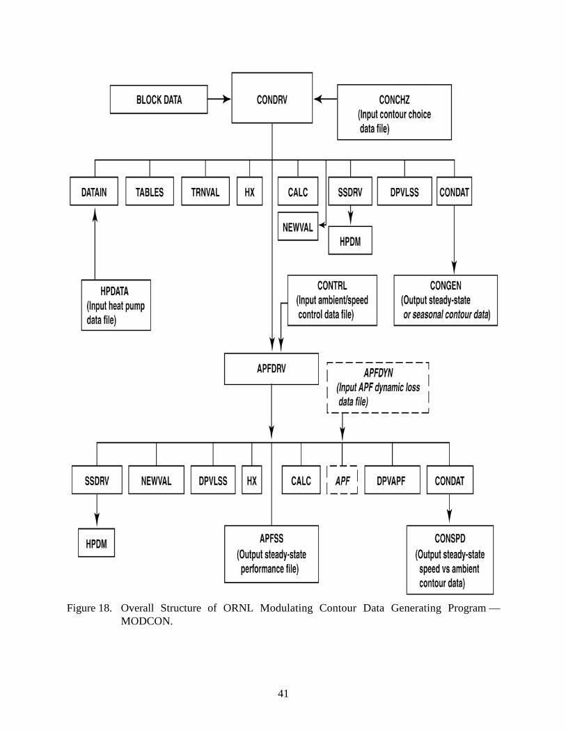
41
Figure 18. Overall Structure of ORNL Modulating Contour Data Generating Program —MODCON.

42
Figure 19. Detailed Structure of ORNL Modulating Heat Pump Design Model.

43
Figure 20. Structure of Thermodynamic Supporting Routines for Refrigerant and Air Properties.

44
Under the flow rate and ambient variables heading the following categories are covered:
• nominal refrigerant and air flows,
• nominal compressor and fan motor sizing,
• refrigerant- and air-side modulation variables,
• refrigerant flow/charge control, and
• air-side conditions
Twenty-five of the 52 independent design variables are in these categories. The remaining 27 areheat exchanger area variables either —
• with total area changing
— such as frontal areas, number of rows, fin pitch, or— total area multipliers — with constant fan power maintained
• or with total area fixed
— either with the indoor to outdoor area-split held constant – by making individual coil tradeoffs with two parameters varying
— or with the area-split changing– by making tradeoffs over both coils with one, two, or three
heat exchanger parameters varying
A listing of the individual parameters available for independent control are given in Table A.2 of theinput data description to the CONCHZ data file in Appendix A.
Operational Control Relationships. When either of the selected pair of independent parametersare ambient temperature or compressor speed, the user can simultaneously adjust up to 5 additionalcontrol variables. The available control variables are:
• compressor inlet superheat,• condenser exit subcooling,• indoor blower frequency,• outdoor fan frequency, or• building load.
User-defined operational control relationships can be defined in either the CONCHZ or theCONTRL input data sets as linear functions of compressor frequency and/or ambient temperature.

45
Heat Pump Model Output Choices. The user selects in the CONCHZ routine which of the morethan 100 available model output values to include in the generated contour data file. The availableoutput parameters are included in Table A.3 of Appendix A. The available categories of data includethe following:
• general heat pump performance data(COPs, EERs, total and sensible capacities, supply air temperatures)
• heat pump power requirements(total, compressor, fans, I2R)
• refrigerant-side conditions(saturation temperatures, flow rate, pressure drops, heat transfer coefficients)
• compressor values (speed, torque, efficiencies, motor size)— for the selected compressor— for the base compressor— compressor drive conversion factors
• indoor coil and blower values(flow rate, speed, torque, efficiencies, motor size, air-side heat transfer and pressure drop)
• outdoor coil and fan values(flow rate, speed, torque, efficiencies, motor size, air-side heat transfer and pressure drop)
• charge and flow control requirements
• flow control parameters (refrigerant temperatures and superheat and subcooling at potential control locations)
• indoor air-side pressure-drop-related values(indoor-component pressure-drop contributions and required duct size)
• additional derived compressor efficiency values
• additional dehumidification parameters
Up to 15 additional output parameters can be added to the model by the user in subroutine DPVLSSwithout having to increase the array sizes specified within the program.

4No doubt there is also an element of greater openness in the reporting of research on the engine-driven variable-speed units which are not yet commercially marketed — in contrast to the electric-driven field where discussion of variable-speed research is more guarded.
46
MODULATING APPLICATIONS-TO-DATE
The ORNL steady-state heat pump models have been applied to a number of modulating applicationsto date. Somewhat curiously, more outside uses of the models for modulating applications (that wehave been made aware of) have been for engine-driven heat pumps rather than for electric-driven.This can perhaps be attributed in part to the wider availability of variable-speed data for opencompressors than for hermetics.4 This lack of publicly available data for variable-speed hermeticcompressor was a significant factor in the ORNL laboratory testing of various IDIM and SWDIMcompressor drives as reported by Miller (1987, 1988a, 1988b).
Engine-Driven Applications
Stirling-Engine-Driven. Through a DOE Work-For-Others contract with Borg-Warner, ORNLadapted the Mark III HPDM to a variable-speed (1000 to 3000 rpm) Stirling-engine-driven heatpump application. This adaptation was accomplished using proprietary Borg-Warner / Stirling PowerSystems (SPS) engine, compressor, and radiator representations for a 10-ton commercial system. Themodified model was transferred to Borg Warner for their use in system design and control analysisfor the Gas Research Institute (GRI) as reported by Monahan (1986).
Internal-Combustion-Engine-Driven. We also provided the Mark III HPDM to Battelle ColumbusLaboratory for another variable-speed engine-driven heat pump application (again 1000 to 3000 rpm)under development for GRI. The ORNL program was selected by Fischer (1986a) as best suited toBattelle’s needs after review of available heat pump models and modified by their staff to modelresidential internal-combustion, engine-driven gas-fired heat pumps for use in another GRIdevelopment project (Fischer 1986b).
A third variable-speed engine-driven project using the ORNL Mark III model was conducted byRusk et al (1990) of Iowa State University. These researchers combined an extensive internalcombustion model with the ORNL program and reported performance values and trends withambient temperature which agreed well with earlier work reported by others using proprietarymodels.
Electric-Driven Applications
At ORNL, different versions of the modulating model have been used in analytical studies and asan aid in developing and guiding an experimental test plan on a variable-speed breadboard system.
As An Aid To Experimental Testing. Before the breadboard tests described by Miller (1987) wereactually conducted, the modulating model was used to conduct a parametric evaluation of theoptimal control scheme for the selected control variables of indoor and outdoor fan speed, condenser

5As the test unit had a suction-line accumulator, the predicted point of maximum required activecharge was used as the charging condition. At the other conditions of lesser required charge, theaccumulator was sufficient to store the excess.
47
subcooling and flow control openings at appropriate ambient and compressor speed combinations.The charge requirements over the range of conditions planned for the tests were also evaluated.
The predicted control-variable optimums were used to narrow the required test ranges for the controlvariables to those which would most likely bracket the final experimentally determined values. Therange of charge requirements similarly predicted were used to guide the experimental test procedureby indicating under which speed and operating conditions the unit should be charged.5 Using themodel in this manner, the experimental testing required to find the system optimums was minimized.As noted earlier in the section on validation, the model did a credible job of predicting the trends inCOP and capacity — as well as the relative charge requirements of the system.
As A Tool To Determine Potential Performance Levels For Residential Unitary Equipment. Thepresent version of the modulating design tool was used by Rice (1992) in a benchmark analysis topredict the maximum performance potential of a near-term modulating residential-size heat pump.Continuously-variable-speed ECMs were assumed to modulate the compressor and the indoor andoutdoor fans with ambient temperature in conjunction with existing modulating reciprocatingcompressor technology. The modulating heat pump design tool was used to optimize such an ECMBenchmark heat pump using speed ranges and total heat exchanger sizes per-unit-capacity equivalentto that used by the highest-SEER-rated variable-speed unit presently on the market. Parametricsteady-state performance optimization was conducted at a nominal design cooling ambient of 95�F(35�C) and three off-design ambients of 82�F (27.8�C) cooling and 47 and 17�F (8.3 and –8.3�C)heating.
The purpose of this near-term benchmark analysis was two-fold. One purpose was to evaluate thepotential performance improvement predicted by a modulating heat pump model with high-efficiencyheat exchangers and drives and current reciprocating compressor technology. The second was todemonstrate a methodology for using a modulating heat pump design tool for such a system designanalysis.
With regard to the first purpose, a potential increase in steady-state cooling performance rangingfrom 12 to 24% was found depending on the sensible-to-total capacity ratio constraints imposed.Steady-state heating performance improvements of 32 to 39% were also predicted compared to thereference commercially available residential unit.
Relating to the demonstration purpose, the experience with the benchmark analysis suggests that areasonably-optimized modulating system can be obtained using the-four-point design approachpresented there. Comparing this most recent design approach with a black-box optimizationapproach conducted in an earlier assessment of variable-speed potential (Rice and Fischer 1985), itwas found that the present approach was intuitively superior with regard to maintaining engineeringcontrol of the design process and by providing a visual (and tabular) mapping of the designobjectives and constraints about the vicinity of the optimums.
48
As A Tool To Assess Potential Of Variable-Speed-Drives For Commercial Unitary Equipment.The present version of the modulating design tool is also currently being used by an EPRI contractorto assess the potential of existing and advanced variable-speed-drives and control strategies forcommercial air-conditioners and heat pumps. In this analysis, special attention is being given to themotor sizing strategies by making use of the sizing options and the torque mapping capabilitiesunique to the ORNL modulating design tool. Some of these capabilities were demonstratedpreviously by Rice (1988a) where an earlier version of the modulating model was used to determinetorque requirements and potential efficiency levels for modulating drives in both heating and coolingmodes of operation.
USE WITH ALTERNATIVE REFRIGERANTS
The program has been modified to be capable of using the HFC R134a as a refrigerant. Theequations and coding necessary to add R134a using a modified form of the Martin-Hou (Martin1959) equation of state (EOS) were provided by an industry user of the program (Spatz 1990).Correlations for the thermophysical properties needed by the model were also included. (With theseadditions, the model can use EOS coefficients for two variations of the Martin-Hou EOS format.)The available thermodynamic property routines have been described by Kartsounes and Erth (1971)and are shown in Figure 20.
The user input has also been modified in the latest version of the modulating model to specify therefrigerant type directly. This is in anticipation of the increased need to evaluate refrigerantalternatives to R22. Presently, only five refrigerants (R12, R22, R114, R502, and R134a) areavailable to be called directly in the program although thermophysical properties for R11, R13, R21,R23, R113, and C318 are also included in subroutine MUKCP. Use of any of these other refrigerantsin the model requires only that the appropriate thermodynamic EOS constants given by Downing(1974) be added to the TABLES subroutine and that compressor maps for these refrigerants beavailable. The user should be aware that the flow control device models are also somewhat specificto R22, R12, and R502 (in the case of cap tubes and TXVs) and to R22 for short-tube orifices andtherefore condenser subcooling should be specified in lieu of specific devices until the flow controlmodels can be further generalized by the user.
Newer pure or azeotropic refrigerant alternatives to R22 can be added with minimal effort as theirthermodynamic and thermophysical properties become available. Provided that compressorperformance maps are also available for these candidate alternative refrigerants, the program couldbe used to determine their comparative performance in optimally configured-and-controlled single-or variable-speed air-to-air heat pump systems.
MODEL AVAILABILITY
The modulating design tool described in this report is available for use by the HVAC research anddevelopment community. An executable version for MS-DOS personal computers is provided.

49
The source program in FORTRAN can be made available under certain conditions and ismodularized so that manufacturers with proprietary compressor, motor, and/or drive information cancustomize the program to their needs.
The author can be contacted directly (e-mail: [email protected]) regarding specifics on how copiesof the model can be obtained for research and development purposes. It is hoped that the descriptionof the model capabilities in this report and the demonstration in a companion document (Rice 1992)of the use of the modulating design tool for the design of high-efficiency modulating heat pumps willencourage U.S. manufacturers to obtain the program and investigate further its use for this purpose.

50
REFERENCES
Air-Conditioning and Refrigeration Institute. 1989. Standard for Unitary Air-Conditioning and Air-Source Heat Pump Equipment, Standard 210/240-89. Arlington, Virginia
D. T. Beecher and T. J. Fagan, “The Effects of Fin Pattern on the Air-Side Heat Transfer Coefficientin Plate Finned-Tube Heat Exchangers,” ASHRAE Transactions, 93, Pt. 2, 1987.
Dabiri, A. E., 1982. “A Steady-State Computer Simulation Model for Air-To-Air Heat Pumps”,ASHRAE Transactions, 88, Pt. 2, pp. 973–987.
Damasceno, G. S., Goldschmidt, V. W., and Rooke, S. P., 1990. “Comparison of Three Steady-StateHeat Pump Computer Models”, ASHRAE Transactions, 96, Pt. 2.
Damasceno, G. S., Domanski, P.A., Rooke, S. P., Goldschmidt, V. W., 1991. “Refrigerant ChargeEffects On Heat Pump Performance”, ASHRAE Transactions, 97, Pt. 1.
Domanski, P.A., 1985. Personal communication, National Institute of Standards and Technology,Building Equipment Division, Gaithersburg, Maryland, August.
Domanski, P.A., 1986. Modeling Of a Heat Pump Charged With a Non-Azeotropic RefrigerantMixture, NBS Technical Note 1218, National Bureau of Standards / U. S. Department ofCommerce, January.
Domanski, P.A., 1988. Recommended Procedure for Rating and Testing of Variable Speed AirSource Unitary Air Conditioners and Heat Pumps, NBSIR 88-3781, National Bureau ofStandards, May.
Downing, R. C., 1974. “Refrigerant Equations”, ASHRAE Transactions, 80, Pt.2.
Fagan, T. J., Lucheta, R. A., and Beecher, D.T., 1987. Oak Ridge National Laboratory Heat PumpPerformance Prediction Computer Code: Additions and Verification, Westinghouse ResearchReport 87-9J8-MATHP-R1, November.
Fischer, R. D., 1986a. State-of-the-Art Review of Vapor-Compression Heat Pump System Models,Task 2.1-Technical Report, GRI, February 1986.
Fischer, R. D., 1986b. Gas Engine Heat Pump Cycle Analysis, Volume I. Model Description andGeneric Analysis, GRI-86/0235, October.
Fischer, S. K. and Rice, C. K. 1983. The Oak Ridge Heat Pump Models: I. A Steady-State ComputerDesign Model for Air-to-Air Heat Pumps, ORNL/CON-80/R1, August.
Fischer, S. K. and Rice, C. K. 1985. “System Design Optimization and Validation for Single-SpeedHeat Pumps”, ASHRAE Transactions, 91, Pt. 2B, pp. 509–523.

51
Fischer, S. K., Rice, C. K., and Jackson, W. L., 1988. The Oak Ridge Heat Pump Model: Mark IIIVersion Program Documentation, ORNL/TM-10192, Oak Ridge National Laboratory, March.
Gray, D. L. and Webb, R. L., 1986. “Heat Transfer and Friction Correlations for Plate Finned-TubeHeat Exchangers Having Plain Fins,” Proc. Eighth International Heat Transfer Conference, SanFrancisco, Heat Transfer 1986, Vol. 6, pp. 2745–2750, Hemisphere: New York
Hiller, C. C. and Glicksman, L. R., 1976. Improving Heat Pump Performance via CompressorCapacity Control – Analysis and Test, Vols. I and II, MIT Energy Laboratory Report No. MIT-EL 76–001.
Lloyd, J. D., 1987, Personal communication, Emerson Electric Company, Electronic Speed ControlDivision, Hazelwood, Missouri, April.
Kartsounes, G. T. and Erth, R. A., 1971. “Computer Calculation of the Thermodynamic Propertiesof Refrigerants 12, 22, and 502", ASHRAE Transactions, 77, Pt. 2.
Kays, W. M. and London, A. L., 1974. Compact Heat Exchangers, McGraw-Hill, New York.
Martin, J. J., 1959. “Correlations and Equations Used in Calculating Thermodynamic Properties of‘Freon’ Refrigerants”, Thermodynamic and Transport Properties of Gases, Liquids, and Solids,ASME, New York City, p.110.
Makayama, W. and Xu, L. P. , 1983. “Enhanced Fins for Air-Cooled Heat Exchangers -HeatTransfer and Friction Factor Correlations,” Proc. ASME-JSME Thermal Engineering JointConference, Hawaii, March 1983, eds. Yasuo Mori and Wen-Jei Yang, New York.
Miller, W. A. 1987. “Steady-State Refrigerant Flow and Airflow Control Experiments Conductedon a Continuously Variable Speed Air-to-Air Heat Pumps”, ASHRAE Transactions, 93, Pt. 2,pp. 1191–1204.
Miller, W. A. 1988a. “Laboratory Capacity Modulation Experiments, Analyses, and Validation”,Proceedings of the 2nd DOE/ORNL Heat Pump Conference: Research and Development onHeat Pumps for Space Conditioning Applications, CONF-8804100, Washington, D.C., April,pp. 7–21.
Miller, W.A. 1988b. “Modulating Heat Pump Component and Adjustable Speed Drive EfficienciesMeasured In The Laboratory”, ASHRAE Transactions, 94, Pt. 1, pp. 874–891.
Miller, W.A. 1988c. “Laboratory Examination and Seasonal Analyses of the Dynamic Losses for aContinuously Variable Speed Heat Pump”, ASHRAE Transactions, 94, Pt. 2, pp. 1246–1268.
Miller, W.A. 1989. Personal communication, Oak Ridge National Laboratory, Energy Division, OakRidge, Tennessee, January.

52
Monahan, R. E., 1986. Phase 1-B Development of Kinematic Stirling/Rankine Commercial Gas-Fired Heat Pump System , Final Report, GRI-86/0192, July.
Rice, C. K. and Fischer, S. K., 1985. “A Comparative Analysis of Single- and Continuously-Variable-Capacity Heat Pump Concepts”, Proceedings of the DOE/ORNL Heat PumpConference: Research and Development on Heat Pumps for Space Conditioning Applications,CONF-841231, Washington, D. C., pp. 57–65.
Rice, C. K., Fischer, S. K., and Emerson, C. J., 1985. The Oak Ridge Heat Pump Models: II. AnAnnual Performance Factor / Loads Model for Residential Air-Source Heat Pumps, ORNL-CON-160.
Rice, C. K. 1987. “The Effect Of Void Fraction Correlation and Heat Flux Assumption OnRefrigerant Charge Inventory Predictions”, ASHRAE Transactions, 93, Pt. 1, pp. 341–367.
Rice, C. K. 1988a. “Efficiency Characteristics of Speed-Modulated Drives at Predicted TorqueConditions for Air-To Air Heat Pumps”, ASHRAE Transactions, 93, Pt. 1, pp. 341–367.
Rice, C.K. 1988b. “Capacity Modulation Component Characterization and Design ToolDevelopment”, Proceedings of the 2nd DOE/ORNL Heat Pump Conference: Research andDevelopment on Heat Pumps for Space Conditioning Applications, CONF-8804100,Washington, D.C., April, pp. 23–33.
Rice, C.K., 1992. “Benchmark Performance Analysis Of An ECM-Modulated Air-To-Air-HeatPump With Reciprocating Compressor”, ASHRAE Transactions, 97, Pt.1.
Rusk, R. P., Van Gerpen, J. H., Nelson, R. M., Pate, M. B., 1990. “Development And Use Of aMathematical Model Of An Engine-Driven Heat Pump”, ASHRAE Transactions, 96, Pt. 2
Spatz, M., 1990. Personal communication, Allied-Signal Corporation, Buffalo, New York, April.
Young, G. 1990. Personal communication, General Electric, Motor Technology Department, FortWayne, Indiana, October.
Zigler, R. V. 1987. Personal communication, General Electric, Motor Technology Department, FortWayne, Indiana, May

53
APPENDIX A
CONTOUR SELECTION DATA FILE ‘CONCHZ’
Input Data Definitions and Format
Tables A.1 to A.4 describe the input data options for the parametric front-end to the ORNLModulating Heat Pump Model. The input format for the choice of independent and dependentvariables for parametric analysis is first given. This is supplemented by Tables A.2 through A.4which describe the choices of independent and dependent variables which are built into the program.Table A.5 describes the format of the output contour-data-generation file generated by the model forthe parameters selected by the user.
The ‘CONCHZ’ data file must always be the first input file to be read by Unit 5 — the default inputunit number. CONCHZ is followed by the heat pump specification file ‘HPDATA’ — also read byUnit 5 as default. The remaining (optional) input data file ‘CONTRL’ , which is described inAppendix H, has a default unit number of 24. The printed output is sent to unit 6 and the contour-data -generation file as described by Table A.5 is sent to unit 8 by default. All of the default inputand output unit number settings are specified in the BLOCK DATA routine and are described furtherat the beginning of Appendix D and at the end of Appendix E.
Sample Input File (Regular and Annotated)
This section contains regular and annotated listings, Listings A.1 and A.2, respectively, of a sample‘CONCHZ’ data file. The selected example is for a heat pump operating in the heating mode witha compressor frequency range from 180 Hz down to 50 Hz and for an ambient range from 17�F to47�F. All the available dependent variables were selected for this example.
The regular listing represents the data set as directly used by the model while the annotated versionof the same data set is labeled with the variable names as described in Table A.1. The annotatedlisting is provided as a visual reference to users modifying existing data sets.


55
Table A.1. Description of CONCHZ Input Data to MODCON Program
Variable Variable Description Sample ValueName
Selection of Operating Mode(s)
LINE 1 FORMAT(I3)
MODEGN operating mode selector 1= 0, bypass contour data generation front-end (omit remainder of data set)= 1, steady-state heating mode= 2, steady-state cooling mode= 3, annual, with seasonal breakdowns (not yet operational)= 4, steady-state heating and cooling modes (for use with CONTRL.DAT)= 5, steady-state heating, cooling, and annual modes,
with seasonal breakdowns (not yet operational)
Heading Identifiers For Selected Operating Mode(s)
LINE 2 FORMAT(10A8)
MTITLE(J) title heading(s) identifying contour data sets generated for HEATING MODEheating, cooling, and/or annual modes as appropriateJ=1 if MODEGN = 1 or 2,J=1, 2 if MODEGN = 4, orJ=1, 2, 3 if MODEGN = 3 or 5
Selection of X and Y Independent Variables
LINE 3 FORMAT(2I3, 5F10.0)
IDVARX ID number of X independent variable (refer to Table A.2) 18NX number of X values to be evaluated 6XLO minimum value of X variable 7.0XHI maximum value of X variable 57.0XREF(J) X reference point to mark on contour plots where 47.0
J=1 if MODEGN = 1 or 2,J=1, 2 if MODEGN = 4, orJ=1, 2, 3 if MODEGN = 3 or 5
LINE 4 FORMAT(2I3, 5F10.0)
IDVARY ID number of Y independent variable (refer to Table A.2) 21NY number of Y values to be evaluated (set to 0 for 1-D parameters) 6
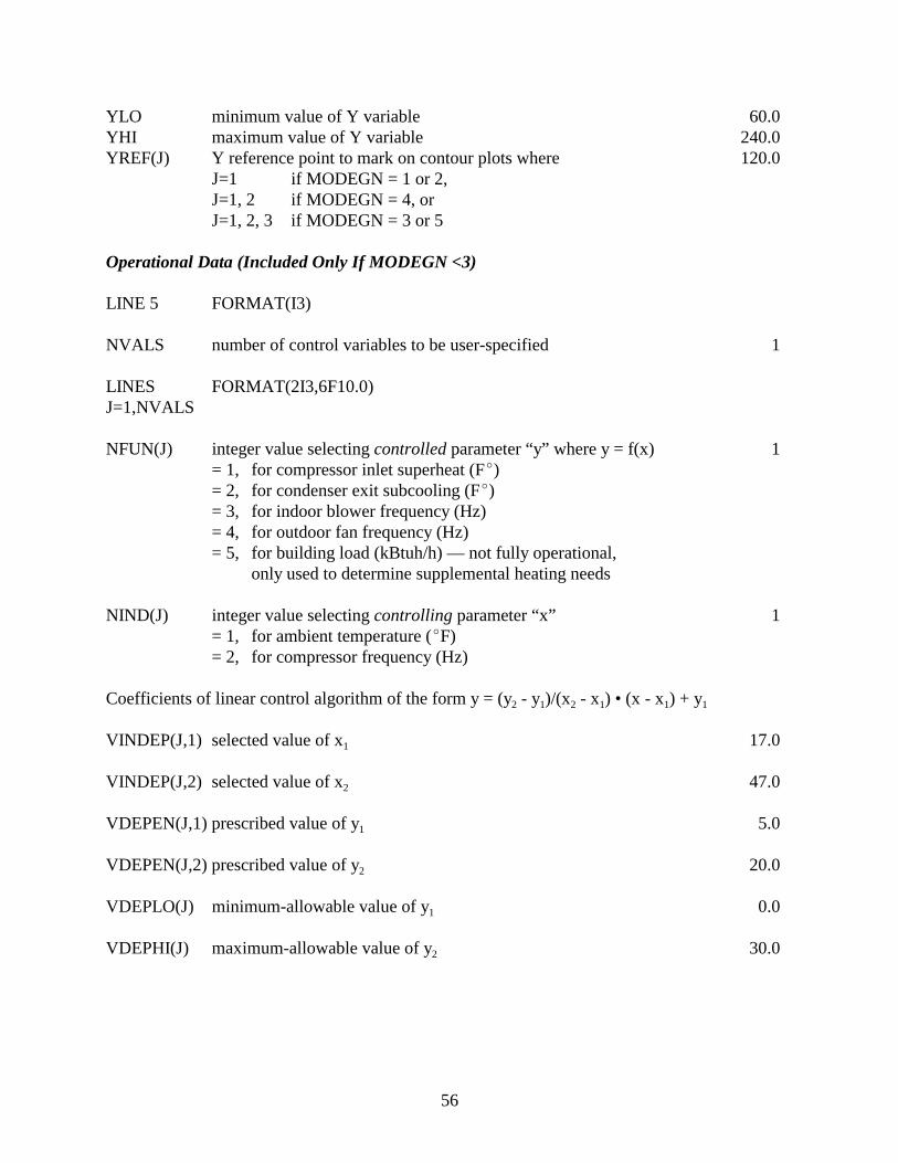
56
YLO minimum value of Y variable 60.0YHI maximum value of Y variable 240.0YREF(J) Y reference point to mark on contour plots where 120.0
J=1 if MODEGN = 1 or 2,J=1, 2 if MODEGN = 4, or J=1, 2, 3 if MODEGN = 3 or 5
Operational Data (Included Only If MODEGN <3)
LINE 5 FORMAT(I3)
NVALS number of control variables to be user-specified 1
LINES FORMAT(2I3,6F10.0)J=1,NVALS
NFUN(J) integer value selecting controlled parameter “y” where y = f(x) 1= 1, for compressor inlet superheat (F�)= 2, for condenser exit subcooling (F�)= 3, for indoor blower frequency (Hz)= 4, for outdoor fan frequency (Hz)= 5, for building load (kBtuh/h) — not fully operational, only used to determine supplemental heating needs
NIND(J) integer value selecting controlling parameter “x” 1= 1, for ambient temperature (�F)= 2, for compressor frequency (Hz)
Coefficients of linear control algorithm of the form y = (y2 - y1)/(x2 - x1) • (x - x1) + y1
VINDEP(J,1) selected value of x1 17.0
VINDEP(J,2) selected value of x2 47.0
VDEPEN(J,1) prescribed value of y1 5.0
VDEPEN(J,2) prescribed value of y2 20.0
VDEPLO(J) minimum-allowable value of y1 0.0
VDEPHI(J) maximum-allowable value of y2 30.0
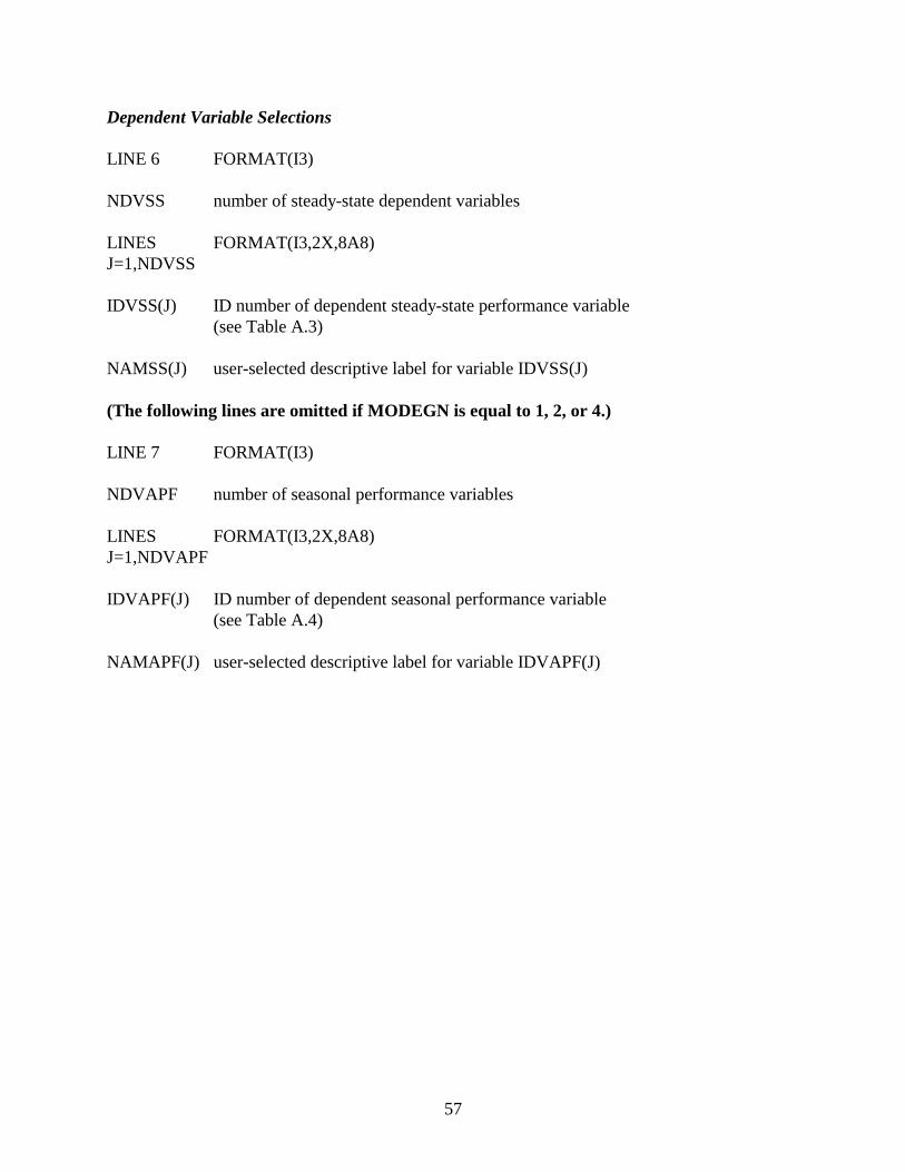
57
Dependent Variable Selections
LINE 6 FORMAT(I3)
NDVSS number of steady-state dependent variables
LINES FORMAT(I3,2X,8A8)J=1,NDVSS
IDVSS(J) ID number of dependent steady-state performance variable (see Table A.3)
NAMSS(J) user-selected descriptive label for variable IDVSS(J)
(The following lines are omitted if MODEGN is equal to 1, 2, or 4.)
LINE 7 FORMAT(I3)
NDVAPF number of seasonal performance variables
LINES FORMAT(I3,2X,8A8)J=1,NDVAPF
IDVAPF(J) ID number of dependent seasonal performance variable (see Table A.4)
NAMAPF(J) user-selected descriptive label for variable IDVAPF(J)


*See the HPDATA input description and the text description accompanying Table 1 for furtherdefinitions of the independent variables.
**Refrigerant circuiting adjusted to hold refrigerant-side pressure drop constant.
59
Table A.2. Key to Independent Contour Variables Availablefor Selection in Input Data File CONCHZ
ID # NAME INDEPENDENT CONTOUR VARIABLE*
Primary Refrigerant/Air Throughput Variables1 DISPL compressor displacement (in3)2 QANMI nominal indoor air flow rate (cfm)3 QANMO nominal outdoor air flow rate (cfm)
Primary Hx Area Variables (Where Total Hx Area Is Allowed To Vary)4 AAFI frontal area of indoor coil (ft2)5 AAFO frontal area of outdoor coil (ft2)6 NTI number of indoor refrigerant tube rows7 NTO number of outdoor refrigerant tube rows8 FPI air-side fin spacing in indoor coil (fins/inch)9 FPO air-side fin spacing in outdoor coil (fins/inch)10** HXMULT total Hx area multiplier relative to baseline values in the
heat pump data file ‘HPDATA’, Hx configurations adjustedto maintain approximately constant fan power requirements
Flow Control Variables11 DTROC refrigerant subcooling at condenser exit (F�)12 TXVRAT capacity of the TXV (tons)13 CAPFLO capillary tube flow factor14 ORIFD diameter of short-tube orifice (in.)
Charge Control Variables15 SUPER compressor inlet superheat (F�)16 REFCHG system refrigerant charge (lbm)
Air-Side-Condition Variables17 TAIII temperature of air entering indoor unit (�F)18 TAIIO temperature of air entering outdoor unit (�F)19 RHII indoor relative humidity20 RHIO outdoor relative humidity
Modulation Variables21 CMPFRQ operating compressor drive frequency (Hz)22 FRQIDF operating indoor blower frequency (Hz)23 FRQODF operating outdoor blower frequency (Hz)24 CFRQRT operating compressor drive frequency ratio (relative to nominal)25 FRQRTI operating indoor fan drive frequency ratio (relative to nominal)26 FRQRTO operating outdoor fan drive frequency ratio (relative to nominal)
Motor Sizing Variables27 CSIZMT nominal motor size for selected compressor (hp)28 SIZMTI nominal indoor blower motor size (hp)29 SIZMTO nominal outdoor fan motor size (hp)

60
Table A.2. Key to Independent Contour Variables Availablefor Selection in Input Data File CONCHZ (continued)
ID # NAME INDEPENDENT CONTOUR VARIABLE
Hx Design Variables (Where Total Hx Area For Both Coils Is Held Constant)
Independent of Total Hx Area30 NSECTI number of equivalent indoor circuits31 NSECTO number of equivalent outdoor circuits32 DDUCT indoor duct size (+in.) or external pressure drop (–in. H2O)
Fixed Area Ratio, Tradeoff Variables For Single Hx’s Holding Individual Hx Area Constant33 NTI (vs AAFI) # of indoor refrigerant tube rows vs frontal area — FPI held constant34 NTO (vs AAFO) # of outdoor refrigerant tube rows vs frontal area — FPO held constant35** FPI (vs AAFI) indoor fin pitch (fins/in) vs frontal area — NTI held constant36** FPO (vs AAFO) outdoor fin pitch (fins/in) vs frontal area — NTO held constant37** FPI (vs NTI) indoor fin pitch (fins/in) vs # of tube rows — AAFI held constant38** FPO (vs NTO) outdoor fin pitch (fins/in) vs # of tube rows — AAFO held constant
Adjustable Area Ratio, Tradeoff Variables Across Hx’s Holding Total Hx Area Constant
One-Variable-Adjustment39** FRACI fraction of total area in indoor coil, frontal area AAFI adjusted and
with AAFI offset by AAFO to maintain fixed total hx area — fixed NT and FP40** FRACO fraction of total area in outdoor coil, frontal area AAFO adjusted and
with AAFO offset by AAFI to maintain fixed total hx area — fixed NT and FP41** FRACI fraction of total area in indoor coil, # of tube rows NTI adjusted and
with NTI offset by NTO to maintain fixed total hx area — fixed AAF and FP42** FRACO fraction of total area in outdoor coil, # of tube rows NTO adjusted and
with NTO offset by NTI to maintain fixed total hx area — fixed AAF and FP43 FRACI fraction of total area in indoor coil, fin spacing FPI adjusted and
with FPI offset by FPO to maintain fixed total hx area — fixed AAF and NT44 FRACO fraction of total area in outdoor coil, fin spacing FPO adjusted and
with FPO offset by FPI to maintain fixed total hx area — fixed AAF and NT
Two-Variable-Adjustment45** FRACI with fraction of total area in indoor coil, AAFI and NTI adjusted and offset
AAFI and NTI by AAFO and NTO to maintain fixed total hx area — fixed FP46** FRACO with fraction of total area in outdoor coil, AAFO and NTO adjusted and offset
AAFO and NTO by AAFI and NTI to maintain fixed total hx area — fixed FP47** FRACI with fraction of total area in indoor coil, AAFI and FPI adjusted and offset
AAFI and FPI by AAFO and FPO to maintain fixed total hx area — fixed NT48** FRACO with fraction of total area in outdoor coil, AAFO and FPO adjusted and offset
AAFO and FPO by AAFI and FPI to maintain fixed total hx area — fixed NT49** FRACI with fraction of total area in indoor coil, NTI and FPI adjusted and offset
NTI and FPI by AAFO and FPO to maintain fixed total hx area — fixed AAF50** FRACO with fraction of total area in outdoor coil, NTO and FPO adjusted and offset
NTO and FPO by AAFI and FPI to maintain fixed total hx area — fixed AAF
Three-Variable-Adjustment (Maintains Approx. Constant Fan Powers)51** FRACI w/NTI, fraction of total area in indoor coil, NTI, AAFI, and FPI adjusted
AAFI and FPI and offset by NTO, AAFO, and FPO to maintain fixed total hx area52** FRACO w/NTO fraction of total area in outdoor coil, NTO, AAFO, and FPO adjusted
AAFO, and FPO and offset by NTI, AAFI, and FPI to maintain fixed total hx area
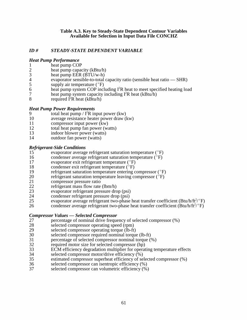
61
Table A.3. Key to Steady-State Dependent Contour VariablesAvailable for Selection in Input Data File CONCHZ
ID # STEADY-STATE DEPENDENT VARIABLE
Heat Pump Performance1 heat pump COP2 heat pump capacity (kBtu/h)3 heat pump EER (BTU/w-h)4 evaporator sensible-to-total capacity ratio (sensible heat ratio — SHR)5 supply air temperature (�F)6 heat pump system COP including I2R heat to meet specified heating load7 heat pump system capacity including I2R heat (kBtu/h)8 required I2R heat (kBtu/h)
Heat Pump Power Requirements9 total heat pump / I2R input power (kw) 10 average resistance heater power draw (kw) 11 compressor input power (kw) 12 total heat pump fan power (watts)13 indoor blower power (watts)14 outdoor fan power (watts)
Refrigerant-Side Conditions15 evaporator average refrigerant saturation temperature (�F)16 condenser average refrigerant saturation temperature (�F)17 evaporator exit refrigerant temperature (�F)18 condenser exit refrigerant temperature (�F)19 refrigerant saturation temperature entering compressor (�F)20 refrigerant saturation temperature leaving compressor (�F)21 compressor pressure ratio22 refrigerant mass flow rate (lbm/h)23 evaporator refrigerant pressure drop (psi)24 condenser refrigerant pressure drop (psi)25 evaporator average refrigerant two-phase heat transfer coefficient (Btu/h/ft2/�F)26 condenser average refrigerant two-phase heat transfer coefficient (Btu/h/ft2/�F)
Compressor Values — Selected Compressor27 percentage of nominal drive frequency of selected compressor (%)28 selected compressor operating speed (rpm)29 selected compressor operating torque (lb-ft)30 selected compressor required nominal torque (lb-ft)31 percentage of selected compressor nominal torque (%)32 required motor size for selected compressor (hp)33 ECM efficiency degradation multiplier for operating temperature effects34 selected compressor motor/drive efficiency (%)35 estimated compressor superheat efficiency of selected compressor (%)36 selected compressor can isentropic efficiency (%)37 selected compressor can volumetric efficiency (%)

62
Table A.3. Key to Steady-State Dependent Contour VariablesAvailable for Selection in Input Data File CONCHZ (continued)
Compressor Values — Base Compressor38 base compressor operating speed (rpm)39 base compressor operating torque (lb-ft)40 base compressor nominal torque (lb-ft)41 percentage of base compressor nominal torque (%)42 base compressor motor/drive efficiency (%)43 base compressor can isentropic efficiency (%)44 base compressor can volumetric efficiency (%)
Compressor Motor Conversion Multipliers45 ratio of selected (converted) to base compressor speed 46 ratio of selected (converted) to base motor/drive efficiency w/o suction gas heating
effects47 estimated suction gas superheating from base compressor motor (F�)48 estimated suction gas superheating from selected compressor motor (F�)49 efficiency multiplier due to differential suction gas heating effects50 mass flow rate multiplier due to differential suction gas heating effects51 ratio of selected (converted) to base motor/drive efficiency with suction gas heating
effects52 ratio of selected (converted) to base refrigerant mass flow rate with suction gas
heating effects 53 ratio of selected (converted) to base compressor power with suction gas heating
effects
Indoor Coil / Blower Values54 indoor air flow rate (cfm)55 indoor blower speed (rpm)56 percentage of nominal indoor blower frequency (%)57 indoor air face velocity (ft/min)58 indoor air surface velocity (ft/min)59 indoor air-side heat transfer coefficient (Btu/h/ft2/�F)60 indoor air-side total pressure drop (in. of H2O)61 indoor coil fin augmentation heat transfer multiplier62 indoor coil fin augmentation pressure drop multiplier63 indoor blower operating torque (oz-ft)64 percentage of selected indoor motor nominal torque (%)65 required nominal size of selected indoor motor (hp)66 motor/drive efficiency of selected indoor drive (%)67 motor/drive efficiency of base indoor drive (%)68 combined blower/motor/drive efficiency of selected indoor blower (%)
Outdoor Coil / Fan Values69 outdoor air flow rate (cfm)70 outdoor fan speed (rpm)71 percentage of nominal outdoor fan frequency (%)72 outdoor air face velocity (ft/min)73 outdoor air surface velocity (ft/min)74 outdoor air-side heat transfer coefficient (Btu/h/ft2/�F)75 outdoor air-side total pressure drop (in. of H2O)
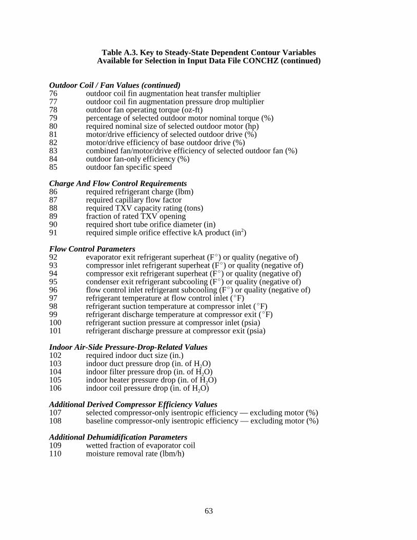
63
Table A.3. Key to Steady-State Dependent Contour VariablesAvailable for Selection in Input Data File CONCHZ (continued)
Outdoor Coil / Fan Values (continued)76 outdoor coil fin augmentation heat transfer multiplier77 outdoor coil fin augmentation pressure drop multiplier78 outdoor fan operating torque (oz-ft)79 percentage of selected outdoor motor nominal torque (%)80 required nominal size of selected outdoor motor (hp)81 motor/drive efficiency of selected outdoor drive (%)82 motor/drive efficiency of base outdoor drive (%)83 combined fan/motor/drive efficiency of selected outdoor fan (%)84 outdoor fan-only efficiency (%) 85 outdoor fan specific speed
Charge And Flow Control Requirements86 required refrigerant charge (lbm)87 required capillary flow factor88 required TXV capacity rating (tons)89 fraction of rated TXV opening90 required short tube orifice diameter (in)91 required simple orifice effective kA product (in2)
Flow Control Parameters92 evaporator exit refrigerant superheat (F�) or quality (negative of)93 compressor inlet refrigerant superheat (F�) or quality (negative of)94 compressor exit refrigerant superheat (F�) or quality (negative of)95 condenser exit refrigerant subcooling (F�) or quality (negative of)96 flow control inlet refrigerant subcooling (F�) or quality (negative of)97 refrigerant temperature at flow control inlet (�F)98 refrigerant suction temperature at compressor inlet (�F)99 refrigerant discharge temperature at compressor exit (�F)100 refrigerant suction pressure at compressor inlet (psia)101 refrigerant discharge pressure at compressor exit (psia)
Indoor Air-Side Pressure-Drop-Related Values102 required indoor duct size (in.)103 indoor duct pressure drop (in. of H2O)104 indoor filter pressure drop (in. of H2O)105 indoor heater pressure drop (in. of H2O)106 indoor coil pressure drop (in. of H2O)
Additional Derived Compressor Efficiency Values107 selected compressor-only isentropic efficiency — excluding motor (%)108 baseline compressor-only isentropic efficiency — excluding motor (%)
Additional Dehumidification Parameters109 wetted fraction of evaporator coil110 moisture removal rate (lbm/h)


65
Table A.4. Key to Seasonal Dependent Contour VariablesAvailable for Selection in Input Data File CONCHZ
(Not Yet Available)
ID # SEASONAL DEPENDENT VARIABLE
1 heating seasonal performance factor2 cooling seasonal performance factor3 annual performance factor4 heating seasonal energy load (kBtuh)5 cooling seasonal energy load (kBtuh)6 annual energy load (kBtuh)7 heating seasonal energy use (kWh or kBtuh)8 cooling seasonal energy use (kWh or kBtuh)9 annual energy use (kWh or kBtuh)10 heating seasonal parasitic energy use (kWh)11 cooling seasonal parasitic energy use (kWh)12 annual parasitic energy use (kWh)13 heating operating time (h)14 cooling operating time (h)15 annual operating time (h)16 supplemental heating energy use (kWh or kBtuh)17 defrost tempering energy use (kWh or kBtuh)18 defrost heat pump energy use (kWh or kBtuh)19 total defrost time (h)20 total number of defrosts


67
Table A.5. Description of Output Contour Data File From MODCON
Identifying Name for Data Set:RECORD 1 FORMAT (80A)
MTITLE data set identifier from line 2 of CONCHZ input data
Independent Variable (Parametric) Data:
Identification of X and Y Independent Variables
X-DataRECORD 2 FORMAT (2I3, 3F10.2)
IDVARX identifying ID number of X independent variable (refer to Table A.2)NX number of X values to be evaluatedXLO minimum value of X variableXHI maximum value of X variableXREF X coordinate of any specified reference point (to mark on contour plot)
Y-DataRECORD 3 FORMAT (2I3, 3F10.2)
IDVARY identifying ID number of Y independent variable (refer to Table A.2)NY number of Y values to be evaluatedYLO minimum value of Y variableYHI maximum value of Y variableYREF Y coordinate of any specified reference point (to mark on contour plot)
Dependent Variable (Performance) Data:
Number of Data SetsRECORD 4 FORMAT (I3)
NDVAR number of dependent variables for which data are generated
Records 5 and 6 are generated for each dependent variable (J = 1, NDVAR).
Identification of Dependent VariableRECORD 5 FORMAT (I3, 2X, 75A)
IDVARD(J) identifier number for dependent variable NAMDEP(J) descriptive label for dependent variable
Values of Dependent VariableRECORD 6 FORMAT (1P, 6E13.5)
VALDEP —> (IX, IY, IDVARD(J)) array of function values stored as vectorswith the X subscript increasing most rapidly and the Y subscript increasing least rapidly going from left to right and top to bottom, respectively.A new line starts each time the Y subscript changes.


69
Listing A.1. Sample Contour Selection Data File ‘CONCHZ’ —
File: H2118V.CHZ
01HEATING MODE PARAMETRIC EVALUATION — COMPRESSOR FREQUENCY VERSUS AMBIENT 21 06 180.0 50.0 180.0 18 03 17.0 47.0 47.0 05 1 2 50.0 180.0 1.0 1.0 1.0 1.0 2 2 50.0 180.0 10.0 24.0 10.0 24.0 3 2 50.0 180.0 64.8 95.0 64.8 95.0 4 2 50.0 180.0 37.1 55.3 37.1 55.3 5 1 17.0 62.0 20.0 0.0 0.0 50.0 110 1 Heat Pump COP 2 Heat Pump Capacity (KBtu/H) 3 Heat Pump EER (BTU/W-H) 4 Evaporator Sensible-To-Total Capacity Ratio 5 Supply Air Temperature (F) 6 Heat Pump System COP With I2R Heat To Meet Specified Heating Load 7 Heat Pump System Capacity Including I2R Heat (KBtu/H) 8 Required I2R Heat (KBtu/H) 9 Total Heat Pump/I2R Input Power (Kw) 10 Average Resistance Heater Power Draw (Kw) 11 Compressor Input Power (Kw) 12 Total Heat Pump Fan Power (Watts) 13 Indoor Blower Power (Watts) 14 Outdoor Fan Power (Watts) 15 Evaporator Average Refrigerant Saturation Temperature (F) 16 Condenser Average Refrigerant Saturation Temperature (F) 17 Evaporator Exit Refrigerant Temperature (F) 18 Condenser Exit Refrigerant Temperature (F) 19 Refrigerant Saturation Temperature Entering Compressor (F) 20 Refrigerant Saturation Temperature Leaving Compressor (F) 21 Compressor Pressure Ratio 22 Refrigerant Mass Flow Rate (lbm/h) 23 Evaporator Refrigerant Pressure Drop (psi) 24 Condenser Refrigerant Pressure Drop (psi) 25 Evaporator Refrigerant Two-Phase Heat Transfer Coef (Btu/h/ft2/F) 26 Condenser Refrigerant Two-Phase Heat Transfer Coef (Btu/h/ft2/F) 27 Percentage Of Nominal Drive Frequency Of Selected Compressor (%) 28 Selected Compressor Operating Speed (rpm) 29 Selected Compressor Operating Torque (lb-ft) 30 Selected Compressor Required Nominal Torque (lb-ft) 31 Percentage Of Selected Compressor Nominal Torque (%) 32 Required Motor Size For Selected Compressor (Hp) 33 ECM Efficiency Degradation Multiplier For Operating Temp Effects

70
Listing A.1. Sample Contour Selection Data File ‘CONCHZ’ —(continued)
34 Selected Compressor Motor/Drive Efficiency (%) 35 Estimated Compressor Superheat Efficiency Of Selected Comp (%) 36 Selected Compressor Can Isentropic Efficiency (%) 37 Selected Compressor Can Volumetric Efficiency (%) 38 Base Compressor Operating Speed (rpm) 39 Base Compressor Operating Torque (lb-ft) 40 Base Compressor Nominal Torque (lb-ft) 41 Percentage Of Base Compressor Nominal Torque (%) 42 Base Compressor Motor/Drive Efficiency (%) 43 Base Compressor Can Isentropic Efficiency (%) 44 Base Compressor Can Volumetric Efficiency (%) 45 Ratio Of Selected To Base Compressor Speed 46 Ratio Of Selected To Base Motor/Drive Efficiency W/O SGH Effects 47 Estimated Suction Gas Superheating From Base Compressor Motor (F) 48 Estimated Suction Gas Superheating From Selected Comp. Motor (F) 49 Efficiency Multiplier Due To Differential SGH Effects 50 Mass Flow Rate Multiplier Due To Differential SGH Effects 51 Ratio Of Selected To Base Motor/Drive Efficiency With SGH Effects 52 Ratio Of Selected To Base Refrig. Mass Flow Rate With SGH Effects 53 Ratio Of Selected To Base Compressor Power With SGH Effects 54 Indoor Air Flow Rate (cfm) 55 Indoor Blower Speed (rpm) 56 Percentage Of Nominal Indoor Blower Frequency (%) 57 Indoor Air Face Velocity (ft/min) 58 Indoor Air Surface Velocity (ft/min) 59 Indoor Air-Side Heat Transfer Coefficient (Btu/h/ft2/F) 60 Indoor Air-Side Pressure Drop (In Of H2O) 61 Indoor Coil Fin Patternation Heat Transfer Multiplier 62 Indoor Coil Fin Patternation Pressure Drop Multiplier 63 Indoor Blower Operating Torque (oz-ft) 64 Percentage Of Selected Indoor Motor Nominal Torque (%) 65 Required Nominal Size Of Selected Indoor Motor (Hp) 66 Motor/Drive Efficiency Of Selected Indoor Drive (%) 67 Motor/Drive Efficiency Of Base Indoor Drive (%) 68 Combined Blower/Motor/Drive Efficiency Of Selected Indoor Blower (%) 69 Outdoor Air Flow Rate (cfm) 70 Outdoor Fan Speed (rpm) 71 Percentage Of Nominal Outdoor Fan Frequency (%) 72 Outdoor Air Face Velocity (ft/min) 73 Outdoor Air Surface Velocity (ft/min) 74 Outdoor Air-Side Heat Transfer Coefficient (Btu/h/ft2/F) 75 Outdoor Air-Side Pressure Drop (In Of H2O) 76 Outdoor Coil Fin Patternation Heat Transfer Multiplier 77 Outdoor Coil Fin Patternation Pressure Drop Multiplier 78 Outdoor Fan Operating Torque (oz-ft) 79 Percentage Of Selected Outdoor Motor Nominal Torque (%) 80 Required Nominal Size Of Selected Outdoor Motor (Hp)

71
Listing A.1. Sample Contour Selection Data File ‘CONCHZ’ —(continued)
81 Motor/Drive Efficiency Of Selected Outdoor Drive (%) 82 Motor/Drive Efficiency Of Base Outdoor Drive (%) 83 Combined Fan/Motor/Drive Efficiency Of Selected Outdoor Fan (%) 84 Outdoor Fan-Only Efficiency (%) 85 Outdoor Fan Specific Speed 86 Required Refrigerant Charge (lbm) 87 Required Capillary Flow Factor 88 Required TXV Capacity Rating (tons) 89 Fraction Of Rated TXV Opening 90 Required Short Tube Orifice Diameter (In) 91 Required Simple Orifice Effective KA Product (In2) 92 Evaporator Exit Refrigerant Superheat (F) Or Quality (–) 93 Compressor Inlet Refrigerant Superheat (F) Or Quality (–) 94 Compressor Exit Refrigerant Superheat (F) Or Quality (–) 95 Condenser Exit Refrigerant Subcooling (F) Or Quality (–) 96 Flow Control Inlet Refrigerant Subcooling (F) Or Quality (–) 97 Refrigerant Temperature At Flow Control Inlet (F) 98 Refrigerant Suction Temperature At Compressor Inlet (F) 99 Refrigerant Discharge Temperature At Compressor Exit (F)100 Refrigerant Suction Pressure At Compressor Inlet (psia)101 Refrigerant Discharge Pressure At Compressor Exit (psia)102 Required Indoor Duct Size (Inches)103 Indoor Duct Pressure Drop (Inches of Water) 104 Indoor Filter Pressure Drop (Inches of Water) 105 Indoor Heater Pressure Drop (Inches of Water) 106 Indoor Coil Pressure Drop (Inches of Water) 107 Selected Compressor-Only Isentropic Efficiency — Excluding Motor (%)108 Baseline Compressor-Only Isentropic Efficiency — Excluding Motor (%)109 Wetted Fraction of Evaporator Coil110 Moisture Removal Rate (lbm/h)

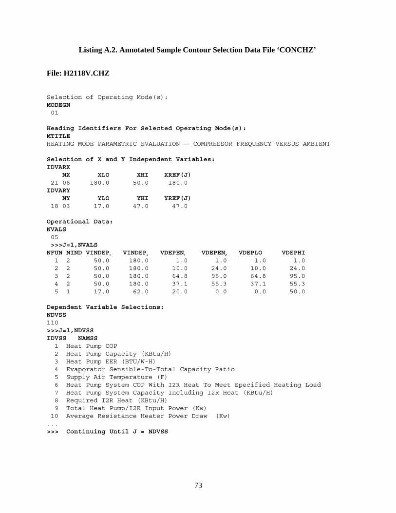
73
Listing A.2. Annotated Sample Contour Selection Data File ‘CONCHZ’
File: H2118V.CHZ
Selection of Operating Mode(s):MODEGN 01
Heading Identifiers For Selected Operating Mode(s):MTITLEHEATING MODE PARAMETRIC EVALUATION — COMPRESSOR FREQUENCY VERSUS AMBIENT
Selection of X and Y Independent Variables: IDVARX NX XLO XHI XREF(J) 21 06 180.0 50.0 180.0IDVARY NY YLO YHI YREF(J) 18 03 17.0 47.0 47.0
Operational Data:NVALS 05 >>>J=1,NVALSNFUN NIND VINDEP1 VINDEP2 VDEPEN1 VDEPEN2 VDEPLO VDEPHI 1 2 50.0 180.0 1.0 1.0 1.0 1.0 2 2 50.0 180.0 10.0 24.0 10.0 24.0 3 2 50.0 180.0 64.8 95.0 64.8 95.0 4 2 50.0 180.0 37.1 55.3 37.1 55.3 5 1 17.0 62.0 20.0 0.0 0.0 50.0
Dependent Variable Selections:NDVSS110>>>J=1,NDVSSIDVSS NAMSS 1 Heat Pump COP 2 Heat Pump Capacity (KBtu/H) 3 Heat Pump EER (BTU/W-H) 4 Evaporator Sensible-To-Total Capacity Ratio 5 Supply Air Temperature (F) 6 Heat Pump System COP With I2R Heat To Meet Specified Heating Load 7 Heat Pump System Capacity Including I2R Heat (KBtu/H) 8 Required I2R Heat (KBtu/H) 9 Total Heat Pump/I2R Input Power (Kw) 10 Average Resistance Heater Power Draw (Kw)...>>> Continuing Until J = NDVSS


75
APPENDIX B
HEAT PUMP SPECIFICATION DATA FILE ‘HPDATA’
Input Data Definitions and Format
In Table B.1, the input parameters and format requirements for the heat pump specification data fileare described. Changes from the ORNL Mark III Single-Speed Version are denoted by verticalchange bars in the extreme leftmost column.
The new data file format was designed to minimize changes required to update existing Mark III datasets. Most of the new input requirements are additive (either by appending to existing lines or byadding new lines). Extra lines for variable-speed compressors, specific augmented heat exchangersurfaces, charge inventory aspects, and convengence tolerances were the main additions. The optionsavailable to some previous entries have also been expanded.
Sample Input Files (Regular and Annotated)
This section contains regular Listings B.1 and B.2 and an annotated Listing B.3 of sample‘HPDATA’ files. The regular listings B.1 and B.2 are for the same heat pump but for differentambient conditions and analysis purposes.
Listing B.1 is a data set appropriate for use in initial design calculations where the compressor andfan motors sizes have not yet been selected. This example data set is for the 95�F design coolingcondition and the motors are to be sized by the model to meet user-specified percentages of nominalloading. The external pressure drop of the indoor duct system has also been specified by the user toimpose a constant value at the design condition.
Listing B.2 is a data set appropriate for use in off-design calculations once the compressor and fanmotors sizes and the indoor duct size have been selected. This example data set is for the 47�F off-design heating condition and the motors and indoor duct system were sized previously by the designcalculation at the 95�F condition.
The changes required to the data sets to switch from a design to an off-design calculation arehighlighted in bold type in Listings B.1 and B.2.
The regular listings represent the data set as directly used by the model while the annotated versionof the first data set is sectioned and labeled with the header types and variable names as describedin Table B.1. The annotated listing is provided as a visual reference to users modifying existing datasets.
The compressor curve-fit coefficients required for the ‘HPDATA’ file can be generated as an outputfile from the compressor map-fitting program described in Appendix G. This output file can beimported into an existing heat pump model data set with minimal editing when a differentcompressor needs to be modeled.

76
The example data set is for a fairly-representative modulating heat pump with total heat exchangersurface area approximately equivalent to that of a present-day commercially-available variable speedunit. The heat exchanger geometry details and compressor are that of a first-generation modulatingheat pump described by Miller (1987, 1988a, 1988b). However, the compressor curve-fits providedare for sine-wave-driven tests of the first-generation-modulating compressor rather than for theinverter-driven case. The sine-wave-driven modulating induction motor data built into the model isfor the same model motor used in the tested compressor. As such, the provided sample-compressor-data is the most consistent baseline for use in assessing the effect of the benefits of advanced drives.

77
Table B.1. Description of HPDATA Input to the MODCON Program
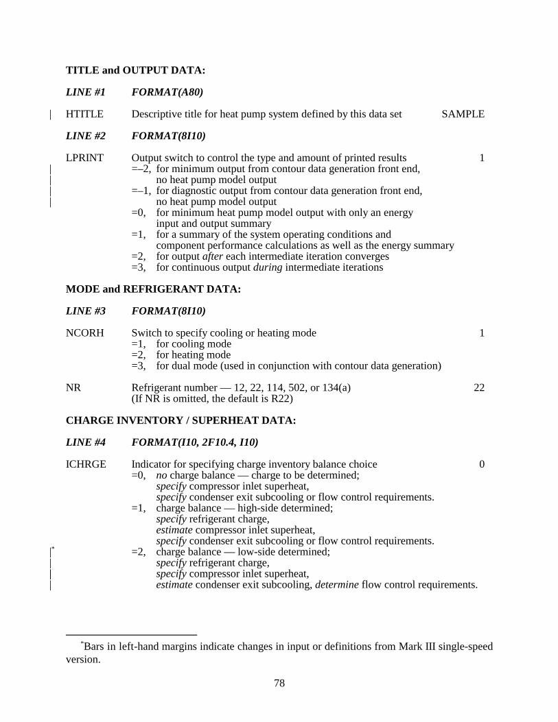
*Bars in left-hand margins indicate changes in input or definitions from Mark III single-speedversion.
78
TITLE and OUTPUT DATA:
LINE #1 FORMAT(A80)
| HTITLE Descriptive title for heat pump system defined by this data set SAMPLE
LINE #2 FORMAT(8I10)
LPRINT Output switch to control the type and amount of printed results 1| =–2, for minimum output from contour data generation front end,| no heat pump model output| =–1, for diagnostic output from contour data generation front end,| no heat pump model output
=0, for minimum heat pump model output with only an energy input and output summary
=1, for a summary of the system operating conditions and component performance calculations as well as the energy summary
=2, for output after each intermediate iteration converges=3, for continuous output during intermediate iterations
MODE and REFRIGERANT DATA:
LINE #3 FORMAT(8I10)
NCORH Switch to specify cooling or heating mode 1=1, for cooling mode=2, for heating mode=3, for dual mode (used in conjunction with contour data generation)
NR Refrigerant number — 12, 22, 114, 502, or 134(a) 22(If NR is omitted, the default is R22)
CHARGE INVENTORY / SUPERHEAT DATA:
LINE #4 FORMAT(I10, 2F10.4, I10)
ICHRGE Indicator for specifying charge inventory balance choice 0=0, no charge balance — charge to be determined;
specify compressor inlet superheat,specify condenser exit subcooling or flow control requirements.
=1, charge balance — high-side determined;specify refrigerant charge,estimate compressor inlet superheat,specify condenser exit subcooling or flow control requirements.
|* =2, charge balance — low-side determined;| specify refrigerant charge,|| specify compressor inlet superheat,| estimate condenser exit subcooling, determine flow control requirements.

*Presently configured only with R-22 surface tension properties.
79
SUPER Specified (if ICHRGE=0,2) or estimated (if ICHRGE=1) 10.0refrigerant superheat (or quality) at the compressor shell inlet (F� or negative of the desired quality fraction)
REFCHG Specified system refrigerant charge (lbm) (8.8)(not needed if ICHRGE=0)
| MVOID Switch to specify heat exchanger void fraction (slip) method 0| for charge inventory calculations| =0, default method — Zivi void fraction model| with analytical solution | for a constant heat flux approximation| >0, various user-selected void fraction models| with variable heat flux effects| (which require slower numerical solutions)| — mass-flow independent methods| =1, Homogeneous (no slip)| =2, Zivi| =3, Lockhart-Martinelli| =4, Thom| =5, Baroczy| — mass-flow dependent methods| =6, Hughmark| =7, Premoli*
| =8, Tandon|| CHARGE INVENTORY CALCULATIONAL DATA:|| LINE #5 FORMAT(I10, 7F10.4)|| IMASS Switch for option to omit refrigerant charge calculations, 1| only active for ICHRGE=0 case| =0, if charge calculations are to be omitted| =1, if charge calculations are to be made|| Compressor and Accumulator Geometry Values for Refrigerant Charge Calculations:| (not required if IMASS = 0 and ICHRGE = 0) | (if an accumulator is not used, set accumulator height ACCHGT to 0.0)|| VOLCMP Internal void space volume of compressor (cu. in.) 395.0|| ACCHGT Height of accumulator (in.) 10.0|| ACCDIA Internal diameter of accumulator (in.) 4.834|| OILDIA Inner diameter of oil return hole J-tube (in.) 0.035

80
| UPPDIA Inner diameter of upper hole in J-tube (in.) 0.040|| HOLDIS Vertical distance between holes (in.) 2.50|| ATBDIA Inner diameter of J-tube (in.) 0.680
FLOW CONTROL DEVICE DATA: (the variables on this line dependon the type of flow control device selected)
LINE #6 FORMAT(I10, 7F10.4)
| Specified or Estimated Condenser Subcooling:|| IREFC =0, for specified or estimated refrigerant subcooling 0| at the condenser exit|| DTROC Specified (if ICHRGE=0,1) or estimated (if ICHRGE=2) 16.0| refrigerant subcooling (or quality) at the condenser exit | (F�or negative of the desired quality fraction)
Thermostatic Expansion Valve:
IREFC =1, for a thermostatic expansion valve (TXV) 1
TXVRAT Rated capacity of the TXV (tons) 2.0
STATIC Static superheat setting for the TXV (F�) 6.0
SUPRAT TXV superheat at rating conditions (F�) 11.0
SUPMAX Maximum effective operating superheat (F�) 13.0
BLEEDF TXV bypass or bleed factor 1.15
NZTBOP Switch to omit TXV nozzle and tube pressure drop calculations 0.0=0.0, to omit tube and nozzle pressure drops=1.0, to include tube and nozzle pressure drop calculations
Capillary Tube:
IREFC =2, for a capillary tube(s) 2
CAPFLO Capillary tube flow factor, see ASHRAE Handbook, 3.8Equipment Vol. (1988), Fig. 39, p. 19.27
NCAP Number of capillary tubes in parallel 1.0
Short Tube Orifice:
IREFC =3, for a short tube orifice 3
ORIFD Diameter of the short-tube orifice (in.) 0.0544

81
ESTIMATES of the LOW- and HIGH-SIDE REFRIGERANT SATURATIONTEMPERATURES:
LINE #7 FORMAT(8F10.4)
TSICMP Estimate of the refrigerant saturation temperature 48.0at the compressor shell inlet (�F)
TSOCMP Estimate of the refrigerant saturation temperature 120.0at the compressor shell outlet (�F)
GENERAL COMPRESSOR DATA:
LINE #8 FORMAT(I10, 7F10.4)
ICOMP Switch to specify which compressor submodel is to be used, 2=1, for the efficiency-and-loss model (single-speed only)=2, for the map-based model (single- or variable-speed)
| DISPL Total piston displacement for selected compressor (cu. in.) 1.70|| CMPSPD Speed/frequency-determining-parameter for selected compressor —|| Operating frequency ratio (relative to nominal frequency on Line 9.1), 1.0| if value � 5 and ICOMP= 2;| Operating drive frequency (Hz), (180.0)| if value > 5 and ICOMP= 2,|
Synchronous compressor motor speed (rpm) (5400.)if ICOMP=1 and FLMOT is specified on LINE #9;
Rated compressor motor speed (rpm) (5250.)if ICOMP=1 and FLMOT is to be calculated
QCAN Compressor shell heat loss rate (Btu/h), 0.0used if CANFAC is 0.0
CANFAC Switch to control the method of specifying 1.0compressor shell heat loss rate, QCAN
=0.0, to specify QCAN explicitly<1.0, to calculate QCAN as a fraction of compressor input power,
POW, (i.e., QCAN = CANFAC * POW)| =1.0, QCAN is based on map submodel of CANFAC| (Map-based model only, Line 9.8)
>1.0, to calculate QCAN from the relationship :QCAN = 0.90 * [1 – {motor * mechanical }] * POW, (only if ICOMP = 1)

82
COMPRESSOR DATA FOR EFFICIENCY-AND-LOSS MODEL: (Lines 9.0 and 9.1)
LINE #9.0 FORMAT(8F10.4)
VR Compressor actual clearance volume ratio 0.06
EFFMMX Maximum efficiency of the compressor motor 0.82
ETAISN Isentropic efficiency of the compressor 0.70
ETAMEC Mechanical efficiency of the compressor 0.80
LINE #9.1 FORMAT(I10, 7F10.4)
MTRCLC Switch to determine whether to calculate the 0full load motor power (FLMOT) or to use the input value
=0, to calculate FLMOT=1, to use the input value of FLMOT
FLMOT Compressor motor output at full load (kW) ( )| (not used if MTRCLC = 0)
QHILO Heat transfer rate from the compressor inlet 300.0line to the inlet gas (Btu/h), used if HILOFC=0.0
HILOFC Switch to determine internal heat transfer 0.0from the high side to the low side, QHILO= 0.0, to specify QHILO explicitly< 1.0, to calculate QHILO = HILOFC * POW� 1.0, to calculate QHILO = 0.03 * POW
OR
| MAP-BASED COMPRESSOR MODEL INPUT DATA:| (Alternative Lines 9.0 through 9.6)|| LINE #9.0 FORMAT(A80)|| CTITLE Descriptive title for map-based compressor data MAP DATA|| LINE #9.1 FORMAT(3I10, 5F10.4)|| MODEDT Switch indicating type of compressor data representation 2| =1, curve fits to compressor input power | and refrigerant mass flow rate| =2, curve fits to compressor shell isentropic| and volumetric efficiencies

83
| ICMPDT Switch identifying drive efficiency level of base compressor data 2
| =0, first-generation inverter-driven induction-motor (IDIM) efficiency| =1, state-of-the-art IDIM efficiency| =2, ideal sine-wave-driven, induction motor (SWDIM) efficiency| =3, electronically-commutated motor (ECM) efficiency|| ICDVCH Switch choosing selected drive efficiency level 3| (to convert base compressor data)
| =0, first-generation IDIM efficiency| =1, state-of-the-art IDIM efficiency| =2, ideal SWDIM efficiency| =3, ECM efficiency|| CSIZMT If > 0.0, nominal motor size for selected compressor (hp), (2.27)| used to determine relative motor loading| and resultant motor efficiency|| If < 0.0, (negative of) specified percentage of nominal loading –130.0| at which the motor efficiency of the selected compressor | is to be evaluated, also (if CMPFRQ = CFRQNM) | the required motor size will be calculated (auto-sizing)|| CFRQNM Nominal frequency for selected motor rating (Hz) 180.0|| CVLTNM Nominal voltage for selected motor rating (Volts) 210.0| — induction motors only|| CVLHZM Selected operating volts/Hertz ratio multiplier (range of 0.85 to 1.15) 1.0| — induction motors only|| LINE #9.2 FORMAT(I10, 7F10.4)|| NHZ Number of frequencies for which compressor-data curve-fits 7| are available,|| DISPLB Base compressor displacement for compressor map (cubic inches) 3.64|| SUPERB Base ‘superheat’ value for compressor map,| If � 0, base superheat entering compressor (F�), 20.0| If < 0, negative of return gas temperature into compressor (�F) (–95.0)|| CSIZMB Motor size for base compressor (hp) 2.75|| CFRQNB Nominal frequency for base motor rating (Hz) 60.0|| CVLTNB Nominal voltage for base motor rating (volts) 210.0| — induction motors only

84
| MAP DATA AT SPECIFIED COMPRESSOR FREQUENCY (HZVAL):|| LINE #9.3 FORMAT(8F10.4)|| HZVAL Compressor frequency value (Hz) for which map data follow 15.0|| RPMVAL Nominal compressor speed at given frequency (rpm) 750.0| (to be used in volumetric efficiency calculations)|| VLTVAL Compressor motor voltage (volts) at given frequency 53.0| for which map data apply — induction motors only|| (If MODEDT = 1 on LINE 9.1)| POWADJ Adjustment factor to curve-fit for power at given frequency 1.0| (set to 1.0 if value is omitted)|| XMRADJ Adjustment factor to curve-fit for mass flow rate at given frequency 1.0| (set to 1.0 if value is omitted)|| (If MODEDT = 2 on LINE 9.1)| ETIADJ Adjustment factor to curve-fit for isentropic efficiency at given frequency 1.0| (set to 1.0 if value is omitted)|| ETVADJ Adjustment factor to curve-fit for volumetric efficiency at given frequency 1.0| (set to 1.0 if value is omitted)|| ( If MODEDT = 1 on Line 9.1, Read Lines 9.4 and 9.5 ) || LINE #9.4 FORMAT(6E10.3)|| CPOWER Coefficients for bi-quadratic fit to compressor power (kW)| as a function of compressor suction and discharge| saturation temperatures (�F), TSICMP and TSOCMP,| of the form —|| POWER(IHZ) = | CPOWER (1,IHZ) * TSOCMP2 + ( )| CPOWER (2,IHZ) * TSOCMP + ( )| CPOWER (3,IHZ) * TSICMP2 + ( )| CPOWER (4,IHZ) * TSICMP + ( )| CPOWER (5,IHZ) * TSOCMP * TSICMP + ( )| CPOWER (6,IHZ) ( )|| LINE #9.5 FORMAT(6E10.3)|| CMASSF Coefficients for bi-quadratic fit | to compressor mass flow rate (lbm/h) | as a function of compressor suction and discharge | saturation temperatures (�F),TSICMP and TSOCMP,| of the form —|

85
| XMR(IHZ) = | CMASSF (1,IHZ) * TSOCMP 2 + ( )| CMASSF (2,IHZ) * TSOCMP + ( )| CMASSF (3,IHZ) * TSICMP 2 + ( )| CMASSF (4,IHZ) * TSICMP + ( )| CMASSF (5,IHZ) * TSOCMP * TSICMP + ( )| CMASSF (6,IHZ) ( )|| (If MODEDT = 2 on Line 9.1, Read Lines 9.6 and 9.7)|| LINE #9.6 FORMAT(6E10.3)|| CETAIS Coefficients for bi-quadratic fit| to compressor shell isentropic efficiency | as a function of compressor suction and discharge | saturation temperatures (�F), TSICMP and TSOCMP,| of the form —| ETAISN(IHZ) =| CETAIS (1,IHZ) * TSOCMP 2 + –2.324E–04| CETAIS (2,IHZ) * TSOCMP + –5.143E–02| CETAIS (3,IHZ) * TSICMP 2 + –2.726E–04| CETAIS (4,IHZ2) * TSICMP + –9.975E–02| CETAIS (5,IHZ) * TSOCMP * TSICMP + 1.515E–03| CETAIS (6,IHZ) 5.760E+00|| LINE #9.7 FORMAT(6E10.3)|| CETAVL Coefficients for curve fit | to compressor shell volumetric efficiency| as a function of pressure ratio PR and discharge pressure PD (psia) | of the form —| ETAVOL(IHZ) =| CETAVL (1,IHZ) * (PR - 1.) + –6.560E+00| CETAVL (2,IHZ) * (PR - 1.) * PD + 7.350E–02| CETAVL (3,IHZ) * (PR - 1.) * PD * PD + –2.192E–04| CETAVL (4,IHZ) 1.176E+00|| (Repeat Lines 9.3 — 9.7 For Each Compressor Frequency, IHZ=1, NHZ)|| Compressor Shell Heat Loss Correlation :|| LINE #9.8 FORMAT(6E10.3)|| CQCAN Coefficients of quadratic fit to compressor shell heat loss | as a function of compressor dischargesaturation temperature (�F) | of the form —| CANFAC =| CQCAN (1) * TSOCMP + –1.704E–02| CQCAN (2) * TSOCMP 2 + 5.610E–05| CQCAN (3) 1.314E+00
(If CANFAC � 1 on Line #8, Line #9.8 must be omitted)

86
INDOOR UNIT DATA:
LINE #10 FORMAT(8F10.4)
Indoor Operating Conditions:
TAIII Air temperature entering the indoor unit (�F) 80.0
RHII Relative humidity of the air entering the indoor unit 0.52
| LINE #11 FORMAT(5F10.4,2I5,2F10.4)|| Indoor Blower:|| FRQIDF Operating frequency parameter for indoor blower —|| if � 5, operating frequency ratio relative to nominal given by FRQNMI 1.0| if > 5, operating frequency (Hz) (108.0)|| FRQNMI Nominal indoor blower frequency (Hz) 108.0|| QANMI Nominal air flow rate (cfm) 900.|| SIZMTI ECM blower motor sizing parameter —| (SIZMTI is only used if ICHIDF=3)|| > 0.0, nominal blower motor size (hp), (0.22)| used to determine relative motor loading| and resultant ECM efficiency|| < 0.0, (negative of) percentage of nominal loading –75.0| at which the ECM efficiency is to be evaluated,| also — if FRQIDF = FRQNMI —
the required motor size will be calculated (auto-sizing)|| FANEFI Fan / fan-motor efficiency parameter —|| � 1.0, specified fixed value of separate or combined| efficiencies of fan and/or drive: | (those values not explicitly specified by FANEFI | will be calculated based on ICHIDF selection)|| If ICHIDF < 0, specified value of (0.335)| combined fan / fan-motor efficiency|| If ICHIDF � 0, specified fan-only efficiency; 0.45|

87
| FANEFI... >1.0, directly-specified power (watts) of reference drive (148.0)| at nominal air flow rate (if available measured| power is not at selected nominal cfm, then ratio| the measured power by cube of cfm ratio),| at reference inlet air temperatures| of 70�F heating and 80�F cooling|| IRFIDF Integer switch to identify reference drive type 3| if FANEFI is used to specify nominal fan power| (only used if FANEFI > 1.0)|| < 0, No reference drive type to be used,| gives a constant implicit drive efficiency with speed|| � 0, Nominal input power is referenced to choice of following drives —| (drive efficiency will vary with speed)| =0, specifies a first-generation IDIM drive| =1, specifies a state-of-the-art IDIM drive| =2, specifies an ideal SWDIM drive| =3, specifies an ECM drive|| ICHIDF Integer switch for choosing selected drive type: 3| For use in combination with given FANEFI values| (If FANEFI � 1.0)| or| For conversion from reference IRFIDF values | to selected ICHIDF drive type| (If FANEFI > 1.0)|| < 0, drive efficiency assumed constant as explicitly | or implicitly given by FANEFI| (If IRFIDF < 0 and FANEFI > 1.0,| ICHIDF will be automatically set to –1)|| � 0, drive efficiency computed using choice of following drives — | (drive efficiency will vary with speed)| =0, specifies a first-generation IDIM drive| =1, specifies a state-of-the-art IDIM drive| =2, specifies an ideal SWDIM drive| =3, specifies an ECM drive
| DDUCT Indoor duct sizing parameter —If > 0, equivalent diameter of each of 6 identical air ducts (in.) (6.20)
— each with an equivalent length of 100 ft | If � 0, (negative of) specified external pressure drop of duct system –0.15| — independent of specified air flow rate or fan speed| (Note: DDUCT is not used in fan power calculations if FANEFI > 1.0)
FIXCAP House heating load (Btu/h), optional, used to calculate 0.0the necessary backup resistance heat in the heating mode

88
LINE #12 FORMAT(8F10.4)
Indoor Heat Exchanger Configuration:
AAFI Frontal (face) area of the coil (sq. ft.) 3.90
NTI Number of refrigerant tube rows in the direction of air flow 4.0
NSECTI Number of equivalent, parallel refrigerant circuits in heat exchanger 3.0
WTI Spacing of the refrigerant tubes in the direction of air flow (in.) 0.866
STI Spacing of the refrigerant tube passes 1.00perpendicular to the direction of air flow (in.)
RTBI Total number of return bends in heat exchanger (all circuits) 128.0
LINE #13.0 FORMAT(8F10.4)
Indoor Heat Exchanger Configuration (continued):
FINTYI Switch to specify the type of fin surface, 2.0=1.0, for smooth fins=2.0, for general wavy (sinusoidal) or zig-zag (corrugated) fins
— using multipliers to smooth fin equations=3.0, for general louvered (simple-strip) fins
— using multipliers to smooth fin equations| =4.0, for specific zig-zag fin designs| =5.0, for specific louvered (simple-strip) fin designs
FPI Fin pitch (fins/in.) 14.0
DELTAI Fin thickness (in.) 0.0050
DEAI Outside diameter of the refrigerant tubes (in.) 0.395
DERI Inside diameter of the refrigerant tubes (in.) 0.371
XKFI Thermal conductivity of the fins (Btu/h-ft-~F) 128.3
XKTI Thermal conductivity of the tubes (Btu/h-ft-~F) 225.0
HCONTI Fraction of the default computed contact conductance 999.999between the fins and tubes
| LINE #14 FORMAT(I10, 7F10.4)|| Fin Patternation Data for Indoor Coil:|| If FINTYI < 4.0, leave a blank line

89
| If FINTYI = 4.0,|| NFPZGI Number of fin patterns per row of tubes in flow direction (integer) 2|| FPDZGI Fin pattern depth (in) 0.045|| If FINTYI = 5.0,|| NSLVI Number of strips in an enhanced zone (integer) (4)|| XLSLVI Length of enhanced louvered zone (mm) (8.0)|| XWSLVI Width of single strip in flow direction (mm) (2.0)|| LINE #15 FORMAT(8F10.4)|| Heat Transfer and Pressure Drop Multipliers for Indoor Coil :|| HTRMLI Refrigerant-side heat transfer multiplier 1.0|| PDRMLI Refrigerant-side pressure-drop multiplier 1.0|| HTAMLI Air-side heat transfer multiplier 1.0|| PDAMLI Air-side coil pressure-drop multiplier 1.0|| CABMLI Air-side system pressure-drop multiplier 1.0|
OUTDOOR UNIT DATA:
LINE #16 FORMAT(8F10.4)
Outdoor Operating Conditions:
TAIIO Air temperature entering the heat exchanger (F) 95.0
RHIO Relative humidity of the air entering the heat exchanger 0.40
| LINE #17 FORMAT(5F10.4,2I5,I10)|| Outdoor Fan:|| FRQODF Operating frequency parameter for outdoor fan —|| if � 5, operating frequency ratio relative to nominal given by FRQNMO 1.0| if > 5, operating frequency (Hz) (82.5)|| FRQNMO Nominal outdoor fan frequency (Hz) 82.5|

90
| QANMO Nominal air flow rate (cfm) 2700.0|| SIZMTO ECM blower motor sizing parameter —| (SIZMTO is only used if ICHODF=3)|| > 0.0, nominal blower motor size (hp), (0.16)| used to determine relative motor loading| and resultant ECM efficiency|| < 0.0, (negative of) percentage of nominal loading –75.0| at which the ECM efficiency is to be evaluated,| also — if FRQODF = FRQNMO — | the required motor size will be calculated (auto-sizing)|| FANEFO Fan / fan motor efficiency parameter —|| � 1.0, specified fixed value of separate or combined| efficiencies of fan and/or drive: | (those values not explicitly specified by FANEFO | will be calculated based on MFANFT / ICHODF selections)|| If MFANFT = 0 and ICHODF < 0, specified value of (0.245)| combined fan / fan motor efficiency|| If MFANFT = 0 and ICHODF � 0, (0.35)| specified fan-only efficiency|| If MFANFT = 1 and ICHODF < 0, (0.70)| specified drive efficiency|| If MFANFT = 1 and ICHODF => 0, 0.00| specified value is ignored, | model calculates both fan and drive efficiencies|| >1.0, directly-specified power (watts) of reference drive 112.0| at nominal air flow rate (if available measured| power is not at selected nominal cfm, then ratio| the measured power by cube of cfm ratio),| at reference inlet air temperatures| of 47�F heating or 95�F cooling|| IRFODF Integer switch to identify reference drive type 3| if FANEFO is used to specify nominal fan power| (only used if FANEFO > 1.0)|| < 0, No reference drive type to be used,| gives a constant implicit drive efficiency with speed|
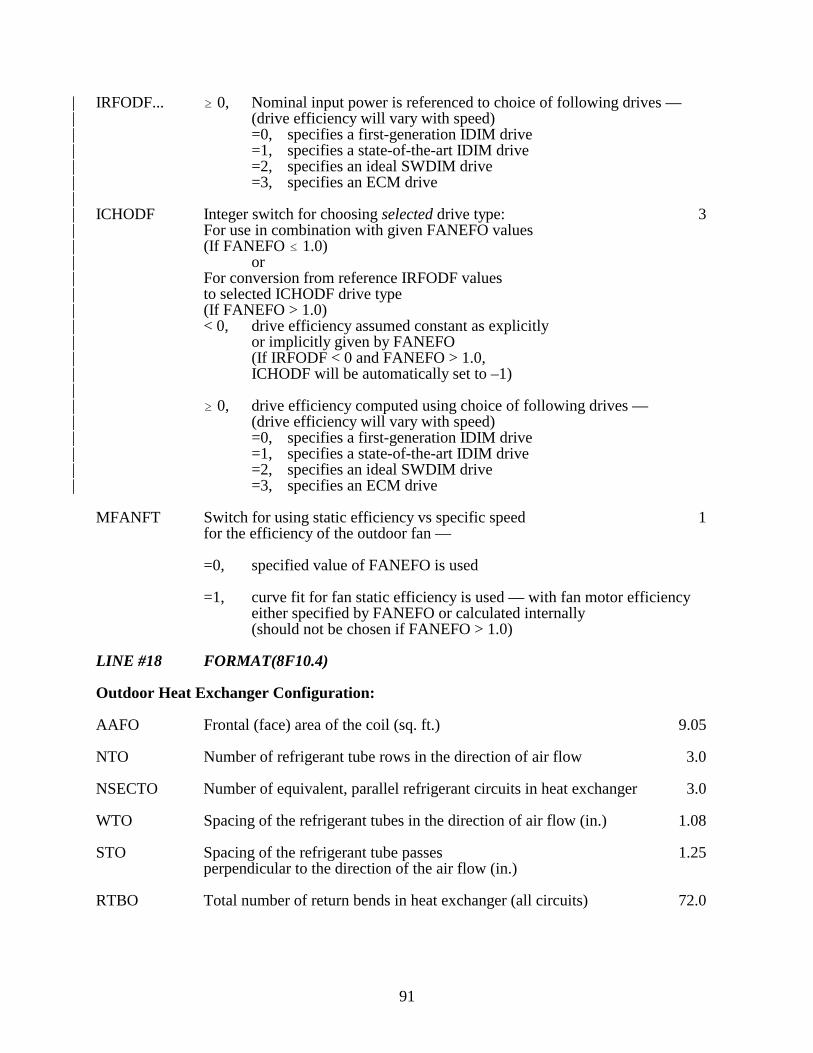
91
| IRFODF... � 0, Nominal input power is referenced to choice of following drives —| (drive efficiency will vary with speed)| =0, specifies a first-generation IDIM drive| =1, specifies a state-of-the-art IDIM drive| =2, specifies an ideal SWDIM drive| =3, specifies an ECM drive|| ICHODF Integer switch for choosing selected drive type: 3| For use in combination with given FANEFO values| (If FANEFO � 1.0)| or| For conversion from reference IRFODF values | to selected ICHODF drive type| (If FANEFO > 1.0)| < 0, drive efficiency assumed constant as explicitly | or implicitly given by FANEFO| (If IRFODF < 0 and FANEFO > 1.0,| ICHODF will be automatically set to –1)|| � 0, drive efficiency computed using choice of following drives — | (drive efficiency will vary with speed)| =0, specifies a first-generation IDIM drive| =1, specifies a state-of-the-art IDIM drive| =2, specifies an ideal SWDIM drive| =3, specifies an ECM drive
MFANFT Switch for using static efficiency vs specific speed 1for the efficiency of the outdoor fan —
=0, specified value of FANEFO is used
=1, curve fit for fan static efficiency is used — with fan motor efficiencyeither specified by FANEFO or calculated internally(should not be chosen if FANEFO > 1.0)
LINE #18 FORMAT(8F10.4)
Outdoor Heat Exchanger Configuration:
AAFO Frontal (face) area of the coil (sq. ft.) 9.05
NTO Number of refrigerant tube rows in the direction of air flow 3.0
NSECTO Number of equivalent, parallel refrigerant circuits in heat exchanger 3.0
WTO Spacing of the refrigerant tubes in the direction of air flow (in.) 1.08
STO Spacing of the refrigerant tube passes 1.25perpendicular to the direction of the air flow (in.)
RTBO Total number of return bends in heat exchanger (all circuits) 72.0

92
LINE #19.0 FORMAT(8F10.4)
Outdoor Heat Exchanger Configuration (continued):
FINTYO Switch to specify the type of fin surface, 2.0=1.0, for smooth fins=2.0, for general wavy (sinusoidal) or zig-zag (corrugated) fins
— using multipliers to smooth fin equations=3.0, for general louvered (simple-strip) fins
— using multipliers to smooth fin equations| =4.0, for specific zig-zag fin designs| =5.0, for specific louvered (simple-strip) fin designs
FPO Fin pitch (fins/in.) 13.0
DELTAO Fin thickness (in.) 0.006
DEAO Outside diameter of the refrigerant tubes (in.) 0.395
DERO Inside diameter of the refrigerant tubes (in.) 0.371
XKFO Thermal conductivity of the fins (Btu/h-ft-�F) 128.3
XKTO Thermal conductivity of the tubes (Btu/h-ft-�F) 225.0
HCONTO Fraction of the default computed contact conductance 999.999between the fins and tubes
Fin Patternation Data for Outdoor Coil:
| LINE # 20 FORMAT(I10, 7F10.4)|| If FINTYO < 4.0, leave a blank line|| If FINTYO = 4.0,|| NFPZGO Number of fin patterns per row of tubes in flow direction (integer) 2|| FPDZGO Fin pattern depth (in.) 0.045|| If FINTYO = 5.0,|| NSLVO Number of strips in an enhanced zone (integer) (4)|| XLSLVO Length of enhanced louvered zone (mm) (8.0)|| XWSLVO Width of single strip in flow direction (mm) (2.0)

93
| LINE #21 FORMAT(8F10.4)|| Heat Transfer and Pressure Drop Multipliers for Outdoor Coil :|| HTRMLO Refrigerant-side heat transfer multiplier 1.0|| PDRMLO Refrigerant-side pressure-drop multiplier 1.0|| HTAMLO Air-side heat transfer multiplier 1.0|| PDAMLO Air — side coil pressure-drop multiplier 1.0|| CABMLO Air — side system pressure-drop multiplier 1.0
CONFIGURATION OPTIONS DATA:
LINE #22 FORMAT(8I10)
MCMPOP Switch for adding compressor can heat loss to air in the outdoor coil 0=0, heat loss not added to outdoor air=1, heat loss added to air before crossing the outdoor coil=2, heat loss added to air after crossing the outdoor coil
MFANIN Switch for adding heat loss from the indoor fan to air stream, 2settings are similar to those for MCMPOP
MFANOU Switch for adding heat loss from the outdoor fan to air stream, 2settings are similar to those for MCMPOP
REFRIGERANT LINES DATA:
LINE #23 FORMAT(8F10.4)
Heat Transfer in Refrigerant Lines :
QSUCLN If > 0, rate of heat gain in the compressor suction line (Btu/h); 100.
If < 0, the negative of the desired temperature rise (–10.)in the suction line (F�)
QDISLN Rate of heat loss in the compressor discharge line (Btu/h) 700.
QLIQLN Rate of heat loss in the liquid line (Btu/h) 700.

94
LINE #24 FORMAT(8F10.4)
Lines Between Coils and from Reversing Valve to Coils:
DLL Inside diameter of the liquid line (in.) 0.2555
XLEQLL Equivalent length of the liquid line (ft.) 39.8
DLRVIC Inside diameter of the vapor line between the reversing valve 0.686and the indoor coil (in.)
XLRVIC Equivalent length of the vapor line between the reversing valve 31.0and the indoor coil (ft.)
DLRVOC Inside diameter of the vapor line between the reversing valve 0.686and the outdoor coil (in.)
XLRVOC Equivalent length of the vapor line between the reversing valve 2.0and the outdoor coil (ft.)
LINE #25 FORMAT(8F10.4)
Lines from the Reversing Valve to the Compressor:
DSLRV Inside diameter of the suction line from the reversing valve 0.793to the compressor inlet (in.)
XLEQLP Equivalent length of the low-pressure line from the reversing valve 5.0to the compressor inlet (ft.)
DDLRV Inside diameter of the discharge line from the compressor outlet 0.561to the reversing valve (in.)
XLEQHP Equivalent length of the high-pressure line from the compressor outlet 2.0to the reversing valve (ft.)

95
| SOLUTION CONVERGENCE CRITERIA :|| LINE #26 FORMAT(8F10.4)|| Iteration Convergence Parameters :|| AMBCON Convergence parameter for the iteration on evaporator inlet air 0.20| temperature (�F)|| CNDCON Convergence parameter for the iteration on condenser exit subcooling 0.20| (or on exit quality * 200) — used when IREFC = 0 on Line 6 (F�);| also the quantity {2 * CNDCON} is used as the convergence parameter | for the charge balancing iteration when ICHRGE =2|| FLOCON Convergence parameter for iteration on refrigerant mass flow rate 0.20| — used when IREFC › 0 on Line 6 (equivalent F�),| value is specified as if it were in degrees F and is scaled| internally (by 1/20th) to give a mass flow convergence factor||| EVPCON Convergence parameter for iteration on evaporator exit superheat (F�), 0.50| (or on exit quality * 500); | Also the quantity {2 * EVPCON} is used as the convergence parameter | for the charge balancing iteration when ICHRGE =1|| CONMST Convergence parameter for iterations on 0.003| evaporator tube wall temperatures in subroutine EVAP | and dew-point temperature in subroutine XMOIST (F�)|| CMPCON Convergence parameter for iteration on suction gas enthalpy 0.05| in the efficiency-and-loss compressor model (Btu/lbm) —| only used when ICOMP = 1 on Line 8|| TOLH Tolerance parameter used by refrigerant routines 0.001| in calculating properties of superheated vapor | when converging on a known enthalpy value (Btu/lbm)|| TOLS Tolerance parameter used by refrigerant routines 0.00005| in calculating properties of superheated vapor | when converging on a known entropy value (Btu/lbm/�R)


97
Listing B.1. Sample Heat Pump Specification File ‘HPDATA’— 95�F Design Cooling Condition —
File: DESIGN.HPS
SAMPLE ECM HEAT PUMP, 95 F DESIGN PT: AUTO-MOTOR + DUCT SIZING, FILE:DESIGN.HPS 1 1 22 0 10.0 0.0 0 1 395.0 10.0 4.834 0.035 0.040 2.5 0.68 0 16.0 0.0 0.0 0.0 0.0 0.0 48.0 120.0 2 1.700 1.0 0.0 1.0SWDIM RECIPROCATING COMPRESSOR — CURVE FITS FROM ORNL AND MANUF’S DATA 2 2 3 -130.0 180.0 210.0 1.0 7 3.64 20.0 2.75 60.0 210.0 15.0000 750.0000 53.0000 1.0 1.0-2.324E-04-5.143E-02-2.726E-04-9.975E-02 1.515E-03 5.760E+00-6.560E+00 7.350E-02-2.192E-04 1.176E+00 20.0000 1050.0000 70.0000 1.0 1.0-5.414E-05-7.267E-04-1.181E-04-3.888E-04 1.387E-04 7.244E-01-5.320E-01 4.385E-03-1.290E-05 9.773E-01 30.0000 1650.0000 107.0000 1.0 1.0-1.209E-04 1.976E-02-6.166E-05-8.747E-04 7.018E-05-3.318E-01-2.101E-01 1.104E-03-3.066E-06 9.595E-01 45.0000 2550.0000 156.0000 1.0 1.0-1.861E-05-3.855E-03-1.039E-04-6.916E-03 1.498E-04 1.004E+00-1.106E-01 3.117E-04-8.162E-07 8.922E-01 60.0000 3450.0000 208.0000 1.0 1.0-7.977E-05 1.039E-02-1.293E-04-9.867E-03 1.840E-04 1.825E-01-1.789E-01 4.585E-04-6.751E-07 9.523E-01 75.0000 4350.0000 208.0000 1.0 1.0-6.626E-06 1.071E-04-4.978E-05-1.304E-03 3.893E-05 5.454E-01-1.445E-01 4.353E-04-7.215E-07 8.580E-01 90.0000 5250.0000 208.0000 1.0 1.0-4.169E-05 7.656E-03-7.209E-05-4.765E-03 7.275E-05 1.228E-01-8.835E-02 1.966E-04-4.783E-07 7.990E-01-1.704E-02 5.610E-05 1.314E+00 80.0 0.52 1.0 108.0 900. -75.0 0.45 3 3 -0.15 0.0 3.900 4.0 3.00 0.866 1.00 128.0 1.0 2.0 14.0 0.0050 0.3950 0.3710 128.3 225.0 999.999 2 0.045 1.0 1.0 1.0 1.0 1.0 95.0 0.40 1.0 82.5 2700.0 -75.0 0.00 3 3 1 9.050 3.0 3.00 1.08 1.25 72.0 1.0 2.0 13.0 0.0060 0.3950 0.3710 128.3 225.0 999.999 3 0.092 1.0 1.0 1.0 1.0 1.0 0 2 2 100. 700. 700. 0.2555 39.8 0.6860 31.00 0.6860 2.00 0.7930 5.00 0.5610 2.00 0.05 0.05 0.40 0.10 0.0015 0.05 0.0005 0.00003


99
Listing B.2. Sample Heat Pump Specification File ‘HPDATA’— 47�F Off-Design Heating Condition —
File : OFFDES.HPS
SAMPLE ECM HEAT PUMP, OFF-DESIGN PT: SPECIFIED MOTORS AND DUCTS, FILE:OFFDES.HPS 1 2 22 0 1.0 0.0 0 1 395.0 10.0 4.834 0.035 0.040 2.5 0.68 0 10.0 0.0 0.0 0.0 0.0 0.0 40.0 100.0 2 1.700 50.0 0.0 1.0SWDIM RECIPROCATING COMPRESSOR — CURVE FITS FROM ORNL AND MANUF’S DATA 2 2 3 2.265 180.0 210.0 1.0 7 3.64 20.0 2.75 60.0 210.0 15.0000 750.0000 53.0000 1.0 1.0-2.324E-04-5.143E-02-2.726E-04-9.975E-02 1.515E-03 5.760E+00-6.560E+00 7.350E-02-2.192E-04 1.176E+00 20.0000 1050.0000 70.0000 1.0 1.0-5.414E-05-7.267E-04-1.181E-04-3.888E-04 1.387E-04 7.244E-01-5.320E-01 4.385E-03-1.290E-05 9.773E-01 30.0000 1650.0000 107.0000 1.0 1.0-1.209E-04 1.976E-02-6.166E-05-8.747E-04 7.018E-05-3.318E-01-2.101E-01 1.104E-03-3.066E-06 9.595E-01 45.0000 2550.0000 156.0000 1.0 1.0-1.861E-05-3.855E-03-1.039E-04-6.916E-03 1.498E-04 1.004E+00-1.106E-01 3.117E-04-8.162E-07 8.922E-01 60.0000 3450.0000 208.0000 1.0 1.0-7.977E-05 1.039E-02-1.293E-04-9.867E-03 1.840E-04 1.825E-01-1.789E-01 4.585E-04-6.751E-07 9.523E-01 75.0000 4350.0000 208.0000 1.0 1.0-6.626E-06 1.071E-04-4.978E-05-1.304E-03 3.893E-05 5.454E-01-1.445E-01 4.353E-04-7.215E-07 8.580E-01 90.0000 5250.0000 208.0000 1.0 1.0-4.169E-05 7.656E-03-7.209E-05-4.765E-03 7.275E-05 1.228E-01-8.835E-02 1.966E-04-4.783E-07 7.990E-01-1.704E-02 5.610E-05 1.314E+00 70.0 0.58 0.6 108.0 900. 0.215 0.45 3 3 6.22 0.0 3.900 4.0 3.00 0.866 1.00 128.0 1.0 2.0 14.0 0.0050 0.3950 0.3710 128.3 225.0 999.999 2 0.045 1.0 1.0 1.0 1.0 1.0 47.0 0.72 0.45 82.5 2700.0 0.157 0.35 3 3 1 9.050 3.0 3.00 1.08 1.25 72.0 1.0 2.0 13.0 0.0060 0.3950 0.3710 128.3 225.0 999.999 3 0.092 1.0 1.0 1.0 1.0 1.0 0 2 2 100. 700. 700. 0.2555 39.8 0.6860 31.00 0.6860 2.00 0.7930 5.00 0.5610 2.00 0.05 0.05 0.40 0.10 0.0015 0.05 0.0005 0.00003


101
Listing B.3. Annotated Sample Heat Pump Specification File ‘HPDATA’— 95�F Design Cooling Condition —
File: DESIGN.HPS
Title and Output Data: ITITLESAMPLE ECM HEAT PUMP, 95 F AMBIENT � DESIGN POINT CALCULATION,FILE:DESIGN.HPS LPRINT 1
Mode and Refrigerant Data: NCORH NR 1 22
Charge Inventory / Superheat Data: ICHRGE SUPER REFCHG MVOID 0 10.0 0.0 0Charge Inventory Calculational Data: IMASS VOLCMP ACCHGT ACCDIA OILDIA UPPDIA HOLDIS ATBDIA 1 395.0 10.0 4.834 0.035 0.040 2.5 0.68
Flow Control Device Data:–>>>IREFC 0 16.0 0.0 0.0 0.0 0.0 0.0 >>>IF =0 DTROC <<<--------------------------------- (Subcooling Control) >>>IF =1 TXVRAT STATIC SUPRAT SUPMAX BLEEDF NZTBOP <<<(TXV) >>>IF =2 CAPFLO NCAP <<<----------------------- (Capillary Tube) >>>IF =3 ORIFD <<<--------------------------------- (Short Tube Orifice)
Estimates of Low- and High-Side Refrigerant Saturation Temperatures: TSICMP TSOCMP 48.0 120.0
General Compressor Data:–>>>ICOMP DISPL CMPSPD QCAN CANFAC 2 1.700 1.0 0.0 1.0Compressor-Model(ICOMP)-Dependent Data: >>>IF =1, <<<----------------------- Loss-and-Efficiency-Based Model Loss-and-Efficiency-Based Compressor Data: VR EFFMMX ETAISN ETAMEC MTRCLC FLMOT QHILO HILOFC >>>IF =2, <<<----------------------- Map-Based Model

102
Listing B.3. Annotated Sample Heat Pump Specification File ‘HPDATA’— 95�F Design Cooling Condition —
(continued)
Compressor-Model(ICOMP)-Dependent Data (continued): Map-Based Compressor Data: CTITLE SWDIM RECIPROCATING COMPRESSOR — CURVE FITS FROM ORNL AND MANUF’S DATA MODEDT ICMPDT ICDVCH CSIZMT CFRQNM CVLTNM CVLHZM 2 2 3 -130.0 180.0 210.0 1.0—>>>>>NHZ DISPLB SUPERB CSIZMB CFRQNB CVLTNB 7 3.64 20.0 2.75 60.0 210.0 >>>IHZ=1,NHZ (POWADJ) (XMRADJ) >>HZVAL RPMVAL VLTVAL ETIADJ ETVADJ 15.0000 750.0000 53.0000 1.0 1.0 >>AND IF MODEDT = 1, CPOWER(1) CPOWER(2) CPOWER(3) CPOWER(4) CPOWER(5) CPOWER(6) CXMR(1) CXMR(2) CXMR(3) CXMR(4) CXMR(5) CXMR(6) >>OR IF MODEDT = 2, CETAIS(1) CETAIS(2) CETAIS(3) CETAIS(4) CETAIS(5) CETAIS(6) CETAVL(1) CETAVL(2) CETAVL(3) CETAVL(4) -2.324E-04-5.143E-02-2.726E-04-9.975E-02 1.515E-03 5.760E+00-6.560E+00 7.350E-02-2.192E-04 1.176E+00 >>>IHZ=2 20.0000 1050.0000 70.0000 1.0 1.0-5.414E-05-7.267E-04-1.181E-04-3.888E-04 1.387E-04 7.244E-01-5.320E-01 4.385E-03-1.290E-05 9.773E-01 >>>IHZ=3 30.0000 1650.0000 107.0000 1.0 1.0-1.209E-04 1.976E-02-6.166E-05-8.747E-04 7.018E-05-3.318E-01-2.101E-01 1.104E-03-3.066E-06 9.595E-01 >>>IHZ=4 45.0000 2550.0000 156.0000 1.0 1.0-1.861E-05-3.855E-03-1.039E-04-6.916E-03 1.498E-04 1.004E+00-1.106E-01 3.117E-04-8.162E-07 8.922E-01 >>>IHZ=5 60.0000 3450.0000 208.0000 1.0 1.0-7.977E-05 1.039E-02-1.293E-04-9.867E-03 1.840E-04 1.825E-01-1.789E-01 4.585E-04-6.751E-07 9.523E-01 >>>IHZ=6 75.0000 4350.0000 208.0000 1.0 1.0-6.626E-06 1.071E-04-4.978E-05-1.304E-03 3.893E-05 5.454E-01-1.445E-01 4.353E-04-7.215E-07 8.580E-01 >>>IHZ=7 90.0000 5250.0000 208.0000 1.0 1.0-4.169E-05 7.656E-03-7.209E-05-4.765E-03 7.275E-05 1.228E-01-8.835E-02 1.966E-04-4.783E-07 7.990E-01 Compressor Shell Heat Loss Correlation: CQCAN(1) CQCAN(2) CQCAN(3) -1.704E-02 5.610E-05 1.314E+00

103
Listing B.3. Annotated Sample Heat Pump Specification File ‘HPDATA’— 95�F Design Cooling Condition —
(continued)
Indoor Unit Data: Indoor Operating Conditions: TAIII RHII 80.0 0.52 Indoor Blower: IRFIDF FRQIDF FRQNMI QANMI SIZMTI FANEFI ^ ICHIDF DDUCT FIXCAP 1.0 108.0 900. -75.0 0.45 3 3 -0.15 0.0 Indoor Heat Exchanger Configuration: AAFI NTI NSECTI WTI STI RTBI 3.900 4.0 3.00 0.866 1.00 128.0–>>FINTYI FPI DELTAI DEAI DERI XKFI XKTI HCONTI 2.0 14.0 0.0050 0.3950 0.3710 128.3 225.0 999.999 Fin Patternation Data for Indoor Coil: >>IF<4.0, NEXT CARD IS NOT USED >>IF=4.0, (specific zig-zag fins) NFPZGI FPDZGI 2 0.045 >>IF=5.0, (specific louvered fins) NSLVI XLSLVI XWSLVI 4 8.0 2.0 Heat Transfer and Pressure Drop Adjustment Multipliers for Indoor Unit: HTRMLI PDRMLI HTAMLI PDAMLI CABMLI 1.0 1.0 1.0 1.0 1.0
Outdoor Unit Data: Outdoor Operating Conditions: TAIIO RHIO 95.0 0.40 Outdoor Blower: IRFODF FRQODF FRQNMO QANMO SIZMTO FANEFO ^ ICHODF MFANFT 1.0 82.5 2700.0 -75.0 0.00 3 3 1 Outdoor Heat Exchanger Configuration: AAFO NTO NSECTO WTO STO RTBO 9.050 3.0 3.00 1.08 1.25 72.0–>>FINTYO FPO DELTAO DEAO DERO XKFO XKTO HCONTO 2.0 13.0 0.0060 0.3950 0.3710 128.3 225.0 999.999 Fin Patternation Data for Outdoor Coil: >>IF<4.0, next card is not used >>IF=4.0, (specific zig-zag fins) NFPZGO FPDZGO 3 0.092 >>IF=5.0, (specific louvered fins) NSLVO XLSLVO XWSLVO 4 8.0 2.0Heat Transfer and Pressure Drop Adjustment Multipliers for Outdoor Unit: HTRMLO PDRMLO HTAMLO PDAMLO CABMLO 1.0 1.0 1.0 1.0 1.0

104
Listing B.3. Annotated Sample Heat Pump Specification File ‘HPDATA’— 95�F Design Cooling Condition —
(continued)
Configuration Options Data: MCMPOP MFANIN MFANOU 0 2 2
Refrigerant Lines Data: Heat Transfer in Refrigerant Lines: QSUCLN QDISLN QLIQLN 100.0 700.0 700.0 Lines Between Coils and from Reversing Valve to Coils: DLL XLEQLL DRVIC XLRVIC DLRVOC XLRVOC 0.2555 39.8 0.6860 31.00 0.6860 2.00 Lines from Reversing Valve to Compressor: DSLRV XLEQLP DDLRV XLEQHP 0.7930 5.00 0.5610 2.00

105
APPENDIX C
SAMPLE PROGRAM RESULTS
Single-Point Cases
Sample program output for single-case runs of the ORNL Modulating Design Tool are shown inListings C.1 and C.2 for the LPRINT = 3 summary output option. These cases are the results ofexecuting the model with the data files DESIGN.HPS and OFFDES.HPS as given in Listings B.1and B.2, respectively, with each file preceded by a null ‘CONCHZ’ data set (a single line with a zeroin column 3) indicating that no parametric analysis was desired. In these cases, no contour datageneration output file is created.
The two cases show, respectively, results for a maximum-speed, cooling-mode, design point casewith auto-motor sizing and a minimum-speed, heating-mode, off-design case with specified motorsizes and indoor duct system. For each run, the new output added since the Mark III single-speedmodel is indicated in bold type. New sections of printed output include a fan/blower performancesection and a tabulation of charge inventory computations by component (the latter as describedearlier in the report in Table CHG1).
Parametric Case
The outputs from an sample parametric analysis case are shown in Listings C.3 and C.4. For this run,the ‘CONCHZ’ data set H2118V.CHZ as given in Listing A.1 and the ‘HPDATA’ fileOFFDES.HPS as given in Listing B.2 were used. The selected example is for a heat pump operatingin the heating mode with a compressor frequency range from 180 Hz down to 50 Hz and for anambient range from 17�F to 47�F. All the available dependent variables were selected to begenerated for this example.
Listing C.3 gives the sample print output which includes a summary of the operational controlparameters specified by the user as a function of compressor frequency and ambient temperature. Inthis example, compressor inlet superheat, condenser outlet subcooling, and indoor and outdoor airflow rates are controlled as functions of compressor frequency and a building heating load line isgiven as a function of ambient temperature. The latter allows effects of resistance heat requirementsto be included in the system power and COP calculations.
Listing C.4 shows an example of the type of parametric sensitivity data sets that can be generatedby the ORNL Modulating Heat Pump Design Tool when the full available parameter list ofdependent variables is chosen. These data sets can be readily exported to PC’s for graphical analysisof selected parameters of interest. The output format of this data file is described in Table A.5.


107
Listing C.1. Sample Single-Point Heat Pump Model Run
— 95�F Design Cooling Condition —
Summary Output


109
***** CONTOUR DATA GENERATION INFORMATION *****
*** CONTOUR DATA GENERATOR FRONT-END IS BYPASSED ***
***** INPUT DATA ***** SAMPLE ECM HEAT PUMP, 95 F DESIGN PT: AUTO-MOTOR + DUCT SIZING, FILE:DESIGN.HPS SUMMARY OUTPUT COOLING MODE OF OPERATION THE REFRIGERANT IS R 22 REFRIGERANT CHARGE IS NOT SPECIFIED COMPRESSOR INLET SUPERHEAT IS SPECIFIED AT 10.00 F
CONDENSER EXIT SUBCOOLING IS SPECIFIED AT 16.00 F
ESTIMATE OF: SATURATION TEMPERATURE INTO COMPRESSOR 48.00 F SATURATION TEMPERATURE OUT OF COMPRESSOR 120.00 F
COMPRESSOR CHARACTERISTICS: OPERATING FREQUENCY RATIO 1.000 TOTAL DISPLACEMENT 1.700 CUBIC INCHES
SWDIM RECIPROCATING COMPRESSOR — CURVE FITS FROM ORNL AND MANUF’S DATA
DRIVE TYPE OF INPUT COMPRESSOR DATA IS SINE-WAVE-DRIVEN DRIVE TYPE IS TO BE CONVERTED TO PM-ECM-DRIVEN
SELECTED PERCENTAGE OF NOMINAL LOADING IS 130.0 % NOMINAL FREQUENCY FOR MOTOR RATING AT 180.0 HZ
BASE SUPERHEAT FOR COMPRESSOR MAP 20.000 F BASE DISPLACEMENT FOR COMPRESSOR MAP 3.640 CU IN
BASE MOTOR SIZE IS 2.75 HP NOMINAL FREQUENCY FOR BASE MOTOR RATING AT 60.0 HZ NOMINAL VOLTAGE FOR BASE MOTOR RATING AT 210.0 VOLTS
***** INPUT DATA *****
— USER PROVIDED COEFFICIENTS FOR COMPRESSOR SHELL ISENTROPIC AND VOLUMETRIC EFFICIENCY —
CURVE FIT REPRESENTATIONS AT 7 DISCRETE FREQUENCIES
CURVE FIT COEFFICIENTS AT 15.0 HZ FREQUENCY NOMINAL SPEED OF 750.0 RPM DRIVE VOLTAGE OF 53.0 VOLTS ISENTROPIC EFF = -2.324E-04*CONDENSING TEMPERATURE**2 + -5.143E-02*CONDENSING TEMPERATURE + -2.726E-04*EVAPORATING TEMPERATURE**2 + -9.975E-02*EVAPORATING TEMPERATURE + 1.515E-03*CONDENSING TEMPERATURE*EVAPORATING TEMPERATURE + 5.760E+00 VOLUMETRIC EFF = -6.560E+00*(PRESSURE RATIO - 1.) + 7.350E-02*(PRESSURE RATIO - 1.)*CONDENSING PRESSURE + -2.192E-04*(PRESSURE RATIO - 1.)*CONDENSING PRESSURE**2 + 1.176E+00

110
CURVE FIT COEFFICIENTS AT 20.0 HZ FREQUENCY NOMINAL SPEED OF 1050.0 RPM DRIVE VOLTAGE OF 70.0 VOLTS ISENTROPIC EFF = -5.414E-05*CONDENSING TEMPERATURE**2 + -7.267E-04*CONDENSING TEMPERATURE + -1.181E-04*EVAPORATING TEMPERATURE**2 + -3.888E-04*EVAPORATING TEMPERATURE + 1.387E-04*CONDENSING TEMPERATURE*EVAPORATING TEMPERATURE + 7.244E-01 VOLUMETRIC EFF = -5.320E-01*(PRESSURE RATIO - 1.) + 4.385E-03*(PRESSURE RATIO - 1.)*CONDENSING PRESSURE + -1.290E-05*(PRESSURE RATIO - 1.)*CONDENSING PRESSURE**2 + 9.773E-01
CURVE FIT COEFFICIENTS AT 30.0 HZ FREQUENCY NOMINAL SPEED OF 1650.0 RPM DRIVE VOLTAGE OF 107.0 VOLTS ISENTROPIC EFF = -1.209E-04*CONDENSING TEMPERATURE**2 + 1.976E-02*CONDENSING TEMPERATURE + -6.166E-05*EVAPORATING TEMPERATURE**2 + -8.747E-04*EVAPORATING TEMPERATURE + 7.018E-05*CONDENSING TEMPERATURE*EVAPORATING TEMPERATURE + -3.318E-01 VOLUMETRIC EFF = -2.101E-01*(PRESSURE RATIO - 1.) + 1.104E-03*(PRESSURE RATIO - 1.)*CONDENSING PRESSURE + -3.066E-06*(PRESSURE RATIO - 1.)*CONDENSING PRESSURE**2 + 9.595E-01
CURVE FIT COEFFICIENTS AT 45.0 HZ FREQUENCY NOMINAL SPEED OF 2550.0 RPM DRIVE VOLTAGE OF 156.0 VOLTS ISENTROPIC EFF = -1.861E-05*CONDENSING TEMPERATURE**2 + -3.855E-03*CONDENSING TEMPERATURE + -1.039E-04*EVAPORATING TEMPERATURE**2 + -6.916E-03*EVAPORATING TEMPERATURE + 1.498E-04*CONDENSING TEMPERATURE*EVAPORATING TEMPERATURE + 1.004E+00 VOLUMETRIC EFF = -1.106E-01*(PRESSURE RATIO - 1.) + 3.117E-04*(PRESSURE RATIO - 1.)*CONDENSING PRESSURE + -8.162E-07*(PRESSURE RATIO - 1.)*CONDENSING PRESSURE**2 + 8.922E-01
CURVE FIT COEFFICIENTS AT 60.0 HZ FREQUENCY NOMINAL SPEED OF 3450.0 RPM DRIVE VOLTAGE OF 208.0 VOLTS ISENTROPIC EFF = -7.977E-05*CONDENSING TEMPERATURE**2 + 1.039E-02*CONDENSING TEMPERATURE + -1.293E-04*EVAPORATING TEMPERATURE**2 + -9.867E-03*EVAPORATING TEMPERATURE + 1.840E-04*CONDENSING TEMPERATURE*EVAPORATING TEMPERATURE + 1.825E-01 VOLUMETRIC EFF = -1.789E-01*(PRESSURE RATIO - 1.) + 4.585E-04*(PRESSURE RATIO - 1.)*CONDENSING PRESSURE + -6.751E-07*(PRESSURE RATIO - 1.)*CONDENSING PRESSURE**2 + 9.523E-01
CURVE FIT COEFFICIENTS AT 75.0 HZ FREQUENCY NOMINAL SPEED OF 4350.0 RPM DRIVE VOLTAGE OF 208.0 VOLTS ISENTROPIC EFF = -6.626E-06*CONDENSING TEMPERATURE**2 + 1.071E-04*CONDENSING TEMPERATURE + -4.978E-05*EVAPORATING TEMPERATURE**2 + -1.304E-03*EVAPORATING TEMPERATURE + 3.893E-05*CONDENSING TEMPERATURE*EVAPORATING TEMPERATURE + 5.454E-01 VOLUMETRIC EFF = -1.445E-01*(PRESSURE RATIO - 1.) + 4.353E-04*(PRESSURE RATIO - 1.)*CONDENSING PRESSURE + -7.215E-07*(PRESSURE RATIO - 1.)*CONDENSING PRESSURE**2 + 8.580E-01
CURVE FIT COEFFICIENTS AT 90.0 HZ FREQUENCY NOMINAL SPEED OF 5250.0 RPM DRIVE VOLTAGE OF 208.0 VOLTS ISENTROPIC EFF = -4.169E-05*CONDENSING TEMPERATURE**2 + 7.656E-03*CONDENSING TEMPERATURE + -7.209E-05*EVAPORATING TEMPERATURE**2 + -4.765E-03*EVAPORATING TEMPERATURE + 7.275E-05*CONDENSING TEMPERATURE*EVAPORATING TEMPERATURE + 1.228E-01 VOLUMETRIC EFF = -8.835E-02*(PRESSURE RATIO - 1.) + 1.966E-04*(PRESSURE RATIO - 1.)*CONDENSING PRESSURE + -4.783E-07*(PRESSURE RATIO - 1.)*CONDENSING PRESSURE**2 + 7.990E-01
GENERAL SHELL HEAT LOSS CORRELATION IS SELECTED: CANFAC = -1.70400E-02*CONDENSING TEMPERATURE + 5.61000E-05*CONDENSING TEMPERATURE**2 + 1.31400E+00
SUPERHEAT CORRECTION TERMS (SET IN BLOCK DATA): SUCTION GAS HEATING FACTOR 0.330 VOLUMETRIC EFFICIENCY CORRECTION FACTOR 0.750 SUCTION SUPERHEAT HEAT TRANSFER FACTOR 0.050 SUCTION GAS HEAT PICKUP FRACTION 0.750

111
**** INPUT DATA *****
INDOOR UNIT: INLET AIR TEMPERATURE 80.000 F RELATIVE HUMIDITY 0.52000 FAN OPERATING FREQUENCY RATIO 1.00 FAN NOMINAL FREQUENCY 108.00 HZ NOMINAL AIRFLOW RATE 900.00 CFM FAN NOMINAL SPEED 1080.00 RPM NUMBER OF MOTOR POLES 12 PERCENT OF NOMINAL LOADING 75.0 % CONSTANT FAN-ONLY EFFICIENCY 0.45 SELECTED FAN DRIVE PM-ECM-DRIVEN SPECIFIED EXTERNAL (DUCT) PRESSURE DROP 0.15 IN H20 FRONTAL AREA OF HX 3.900 SQ FT GENERAL WAVY OR ZIG-ZAG FINS NUMBER OF TUBES IN DIRECTION OF AIR FLOW 4.00 FIN PITCH 14.00 FINS/IN NUMBER OF PARALLEL CIRCUITS 3.00 FIN THICKNESS 0.00500 IN OD OF TUBES IN HX 0.39500 IN THERMAL CONDUCTIVITY: FINS 128.30 BTU/H-FT-F ID OF TUBES IN HX 0.37100 IN THERMAL CONDUCTIVITY: TUBES 225.00 BTU/H-FT-F HORIZONTAL TUBE SPACING 0.866 IN FRACTION OF COMPUTED CONTACT CONDUCTANCE 999.999 VERTICAL TUBE SPACING 1.000 IN NUMBER OF RETURN BENDS 128.00 REF-SIDE HEAT-TRANSFER MULTIPLIER 1.000 AIR-SIDE HEAT-TRANSFER MULTIPLIER 1.000 REF-SIDE PRESSURE-DROP MULTIPLIER 1.000 AIR-SIDE PRESSURE-DROP MULTIPLIER — UNIT 1.000 AIR-SIDE PRESSURE-DROP MULTIPLIER — SYSTEM 1.000
OUTDOOR UNIT: INLET AIR TEMPERATURE 95.000 F RELATIVE HUMIDITY 0.40000 FAN OPERATING FREQUENCY RATIO 1.00 FAN NOMINAL FREQUENCY 82.50 HZ NOMINAL AIRFLOW RATE 2700.00 CFM FAN NOMINAL SPEED 825.00 RPM NUMBER OF MOTOR POLES 12 PERCENT OF NOMINAL LOADING 75.0 % FAN AND DRIVE EFFICIENCY CALCULATED SELECTED FAN DRIVE PM-ECM-DRIVEN FRONTAL AREA OF HX 9.050 SQ FT GENERAL WAVY OR ZIG-ZAG FINS NUMBER OF TUBES IN DIRECTION OF AIR FLOW 3.00 FIN PITCH 13.00 FINS/IN NUMBER OF PARALLEL CIRCUITS 3.00 FIN THICKNESS 0.00600 IN OD OF TUBES IN HX 0.39500 IN THERMAL CONDUCTIVITY: FINS 128.30 BTU/H-FT-F ID OF TUBES IN HX 0.37100 IN THERMAL CONDUCTIVITY: TUBES 225.00 BTU/H-FT-F HORIZONTAL TUBE SPACING 1.080 IN FRACTION OF COMPUTED CONTACT CONDUCTANCE 999.999 VERTICAL TUBE SPACING 1.250 IN NUMBER OF RETURN BENDS 72.00 REF-SIDE HEAT-TRANSFER MULTIPLIER 1.000 AIR-SIDE HEAT-TRANSFER MULTIPLIER 1.000 REF-SIDE PRESSURE-DROP MULTIPLIER 1.000 AIR-SIDE PRESSURE-DROP MULTIPLIER — UNIT 1.000 AIR-SIDE PRESSURE-DROP MULTIPLIER — SYSTEM 1.000 OUTDOOR UNIT: FAN FAN STATIC EFFICIENCY = -3.993E+00 + 4.266E+00 * LOG10(S/1000.) + -1.024E+00 * (LOG10(S/1000.))**2 WHERE SPECIFIC SPEED (S) = FAN RPM * (AIR FLOW CFM**0.5) / (COIL STATIC PRESSURE DROP**0.75) POWER TO THE INDOOR FAN ADDED TO AIR AFTER CROSSING THE INDOOR COIL. POWER TO THE OUTDOOR FAN ADDED TO AIR AFTER CROSSING THE OUTDOOR COIL.

112
***** INPUT DATA *****
LINE HEAT TRANSFER: HEAT GAIN IN SUCTION LINE 100.0 BTU/H HEAT LOSS IN DISCHARGE LINE 700.0 BTU/H HEAT LOSS IN LIQUID LINE 700.0 BTU/H
DESCRIPTION OF CONNECTING TUBING: LIQUID LINE FROM INDOOR TO OUTDOOR HEAT EXCHANGER ID 0.25550 IN EQUIVALENT LENGTH 39.80 FT FROM INDOOR COIL TO REVERSING VALVE FROM OUTDOOR COIL TO REVERSING VALVE ID 0.68600 IN ID 0.68600 IN EQUIVALENT LENGTH 31.00 FT EQUIVALENT LENGTH 2.00 FT FROM REVERSING VALVE TO COMPRESSOR INLET FROM REVERSING VALVE TO COMPRESSOR OUTLET ID 0.79300 IN ID 0.56100 IN EQUIVALENT LENGTH 5.00 FT EQUIVALENT LENGTH 2.00 FT COMPRESSOR AND ACCUMULATOR GEOMETRY DATA: VOLCMP = 395.00 CU IN ACCHGT = 10.00 IN ACCDIA = 4.83 IN ATBDIA = 0.6800 IN OILDIA = 0.035 IN UPPDIA = 0.040 IN HOLDIS = 2.50 IN
ITERATION TOLERANCES : AMBCON 0.050 F CMPCON 0.050 BTU/LBM TOLH 0.00050 BTU/LBM CNDCON 0.050 F FLOCON 0.400 F TOLS 0.00003 BTU/LBM-R EVPCON 0.100 F CONMST 0.002 F
***** CALCULATED HEAT PUMP PERFORMANCE ***** SYSTEM SUMMARY REFRIGERANT SATURATION REFRIGERANT REFRIGERANT REFRIGERANT AIR TEMPERATURE TEMPERATURE ENTHALPY QUALITY PRESSURE TEMPERATURE COMPRESSOR SUCTION LINE INLET 58.980 F 50.583 F 110.529 BTU/LBM 1.0000 99.696 PSIA SHELL INLET 59.876 49.876 110.764 1.0000 98.524 SHELL OUTLET 187.181 115.410 128.517 1.0000 258.800 CONDENSER INLET 179.280 F 115.373 F 126.869 BTU/LBM 1.0000 258.675 PSIA 95.000 F OUTLET 98.865 114.871 38.911 0.0000 256.994 107.948 EXPANSION DEVICE 93.553 F 112.896 F 37.263 BTU/LBM 0.0000 250.436 PSIA EVAPORATOR INLET 54.386 F 54.386 F 37.263 BTU/LBM 0.1400 106.176 PSIA 80.000 F OUTLET 58.980 50.583 110.529 1.0000 99.696 56.861

113
***** CALCULATED HEAT PUMP PERFORMANCE *****
DRIVE FREQUENCIES COMPRESSOR 180.0 HZ CONDENSER FAN 82.5 HZ EVAPORATOR FAN 108.0 HZ
COMPRESSOR PERFORMANCE COMPRESSOR EFFICIENCY COMPRESSOR DRIVE POWER 2.441 KW OVERALL ISENTROPIC 0.5406 REFRIGERANT MASS FLOW RATE 424.806 LBM/H VOLUMETRIC 0.7658 MOTOR OPERATING SPEED 5400.000 RPM AT A PRESSURE RATIO OF 2.627 % OF NOMINAL FREQUENCY 100.00 % MOTOR NOMINAL SIZE REQUIRED 2.265 HP MOTOR OPERATING TORQUE 45.818 OZ-FT DRIVE EFFICIENCY % OF SELECTED NOMINAL TORQUE 130.000 % SELECTED MOTOR/DRIVE 0.8982 % OF BASE NOMINAL TORQUE 146.459 % BASE MOTOR/DRIVE 0.7810 FLOW MULTIPLIER EFFICIENCY MULTIPLIER MOTOR HEAT 1.043 MOTOR HEAT 1.044 OVERALL DRIVE CHANGE 1.161 OVERALL DRIVE CHANGE 1.201 COMPRESSOR SHELL HEAT LOSS 788.339 BTU/H SUPERHEAT CORRECTION TERMS POWER 0.9936 MASS FLOW RATE 1.0183
FAN/BLOWER PERFORMANCE CONDENSER EVAPORATOR AIR FLOW RATE 2700.00 CFM 900.00 CFM FACE VELOCITY 298.34 FT/MIN 230.77 FT/MIN SURFACE VELOCITY 479.81 FT/MIN 417.04 FT/MIN UNIT PRESSURE DROP 0.098 IN H20 0.187 IN H20 DUCT PRESSURE DROP 0.150 IN H20 FILTER PRESSURE DROP 0.072 IN H20 HEATER PRESSURE DROP 0.103 IN H20 TOTAL PRESSURE DROP 0.098 IN H20 0.512 IN H20 MOTOR SPEED 825.00 RPM 1080.00 RPM % OF NOMINAL FREQUENCY 100.00 % 100.00 % DRIVE EFFICIENCY AT OPERATING SPEED 0.788 0.814 FAN MOTOR TORQUE 12.01 OZ-FT 12.55 OZ-FT % OF NOMINAL TORQUE 75.00 % 75.00 % NOMINAL MOTOR SIZE 0.157 HP 0.215 HP
COMBINED DRIVE & FAN EFFICIENCY 0.280 0.366
OUTDOOR FAN PERFORMANCE: SPECIFIC SPEED 243.88 E+03 FAN-ONLY EFFICIENCY 0.355
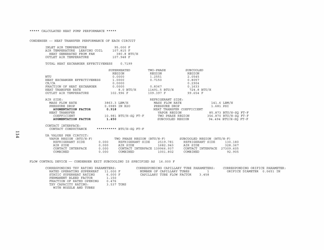
114
***** CALCULATED HEAT PUMP PERFORMANCE *****
CONDENSER — HEAT TRANSFER PERFORMANCE OF EACH CIRCUIT INLET AIR TEMPERATURE 95.000 F AIR TEMPERATURE LEAVING COIL 107.815 F HEAT GENERATED FROM FAN 380.8 BTU/H OUTLET AIR TEMPERATURE 107.948 F
TOTAL HEAT EXCHANGER EFFECTIVENESS 0.7199
SUPERHEATED TWO-PHASE SUBCOOLED REGION REGION REGION NTU 0.0000 1.2551 2.0545 HEAT EXCHANGER EFFECTIVENESS 1.0000 0.7150 0.8057 CR/CA 0.0000 0.2904 FRACTION OF HEAT EXCHANGER 0.0000 0.8367 0.1633 HEAT TRANSFER RATE 8.0 BTU/H 11491.5 BTU/H 724.8 BTU/H OUTLET AIR TEMPERATURE 102.996 F 109.397 F 99.654 F
AIR SIDE: REFRIGERANT SIDE: MASS FLOW RATE 3863.3 LBM/H MASS FLOW RATE 141.6 LBM/H PRESSURE DROP 0.0985 IN H2O PRESSURE DROP 1.681 PSI AUGMENTATION FACTOR 0.918 HEAT TRANSFER COEFFICIENT HEAT TRANSFER VAPOR REGION 85.873 BTU/H-SQ FT-F COEFFICIENT 10.981 BTU/H-SQ FT-F TWO PHASE REGION 356.870 BTU/H-SQ FT-F AUGMENTATION FACTOR 1.450 SUBCOOLED REGION 94.494 BTU/H-SQ FT-F
CONTACT INTERFACE: CONTACT CONDUCTANCE ********** BTU/H-SQ FT-F UA VALUES PER CIRCUIT: VAPOR REGION (BTU/H-F) TWO PHASE REGION (BTU/H-F) SUBCOOLED REGION (BTU/H-F) REFRIGERANT SIDE 0.000 REFRIGERANT SIDE 2519.781 REFRIGERANT SIDE 130.180 AIR SIDE 0.000 AIR SIDE 1682.943 AIR SIDE 328.367 CONTACT INTERFACE 0.000 CONTACT INTERFACE 139966.937 CONTACT INTERFACE 27309.605 COMBINED 0.000 COMBINED 1001.802 COMBINED 92.905
FLOW CONTROL DEVICE — CONDENSER EXIT SUBCOOLING IS SPECIFIED AS 16.000 F CORRESPONDING TXV RATING PARAMETERS: CORRESPONDING CAPILLARY TUBE PARAMETERS: CORRESPONDING ORIFICE PARAMETER: RATED OPERATING SUPERHEAT 11.000 F NUMBER OF CAPILLARY TUBES 1 ORIFICE DIAMETER 0.0651 IN STATIC SUPERHEAT RATING 6.000 F CAPILLARY TUBE FLOW FACTOR 3.458 PERMANENT BLEED FACTOR 1.150 FRACTION OF RATED OPENING 0.476 TXV CAPACITY RATING: 3.537 TONS WITH NOZZLE AND TUBES

115
***** CALCULATED HEAT PUMP PERFORMANCE *****
EVAPORATOR — HEAT TRANSFER PERFORMANCE OF EACH CIRCUIT INLET AIR TEMPERATURE 80.000 F AIR TEMPERATURE LEAVING COIL 56.344 F HEAT GENERATED FROM FAN 504.4 BTU/H OUTLET AIR TEMPERATURE 56.861 F
MOISTURE REMOVAL OCCURS
SUMMARY OF DEHUMIDIFICATION PERFORMANCE (TWO-PHASE REGION)
LEADING EDGE POINT WHERE MOISTURE OF COIL REMOVAL BEGINS LEAVING EDGE OF COIL AIR AIR WALL AIR WALL DRY BULB TEMPERATURE 80.000 F 80.000 F 60.792 F 55.951 F 54.170 F HUMIDITY RATIO 0.01136 0.01136 0.01136 0.00936 0.00891 ENTHALPY 31.696 BTU/LBM 31.696 BTU/LBM 26.975 BTU/LBM 23.617 BTU/LBM 22.696 BTU/LBM
RATE OF MOISTURE REMOVAL 2.5355 LBM/H FRACTION OF EVAPORATOR THAT IS WET 1.0000 LATENT HEAT TRANSFER RATE IN TWO-PHASE REGION 2689. BTU/H SENSIBLE HEAT TRANSFER RATE IN TWO-PHASE REGION 7471. BTU/H SENSIBLE TO TOTAL HEAT TRANSFER RATIO FOR TWO-PHASE REGION 0.7353 OVERALL SENSIBLE TO TOTAL HEAT TRANSFER RATIO 0.7408
OVERALL CONDITIONS ACROSS COIL ENTERING EXITING AIR AIR DRY BULB TEMPERATURE 80.000 F 56.344 F WET BULB TEMPERATURE 67.074 F 55.975 F RELATIVE HUMIDITY 0.520 0.979 HUMIDITY RATIO 0.01136 0.00945
TOTAL HEAT EXCHANGER EFFECTIVENESS (SENSIBLE) 0.8819
SUPERHEATED TWO-PHASE REGION REGION NTU 0.9049 2.3051 HEAT EXCHANGER EFFECTIVENESS 0.5164 0.9002 CR/CA 1.8442 FRACTION OF HEAT EXCHANGER 0.0438 0.9562 HEAT TRANSFER RATE 214.7 BTU/H 10160.3 BTU/H AIR MASS FLOW RATE 58.02 LBM/H 1265.55 LBM/H OUTLET AIR TEMPERATURE 64.923 F 55.951 F

116
EVAPORATOR — HEAT TRANSFER PERFORMANCE OF EACH CIRCUIT
AIR SIDE: REFRIGERANT SIDE: MASS FLOW RATE 1323.6 LBM/H MASS FLOW RATE 141.6 LBM/H PRESSURE DROP 0.512 IN H2O PRESSURE DROP 6.480 PSI AUGMENTATION FACTOR 1.112 HEAT TRANSFER COEFFICIENT HEAT TRANSFER COEFFICIENT DRY COIL 9.196 BTU/H-SQ FT-F VAPOR REGION 71.709 BTU/H-SQ FT-F WET COIL 9.973 BTU/H-SQ FT-F TWO PHASE REGION 702.501 BTU/H-SQ FT-F AUGMENTATION FACTOR 1.450
CONTACT INTERFACE: CONTACT CONDUCTANCE 983204.125 BTU/H-SQ FT-F DRY FIN EFFICIENCY 0.877 WET FIN EFFICIENCY (AVERAGE) 0.814 WET CONTACT FACTOR (AVERAGE) 1.330
UA VALUES PER CIRCUIT:VAPOR TWO PHASE REGION REGION REFRIGERANT SIDE 19.051 4071.052 BTU/H-F AIR SIDE DRY COIL 40.119 0.000 BTU/H-F WET COIL 880.400 BTU/H-F CONTACT INTERFACE DRY COIL 5659.703 0.000 BTU/H-F WET COIL 124081.250 BTU/H-F COMBINED DRY COIL 12.888 0.000 BTU/H-F WET COIL 719.661 BTU/H-F

117
***** SUMMARY OF ENERGY INPUT AND OUTPUT *****
SAMPLE ECM HEAT PUMP, 95 F DESIGN PT: AUTO-MOTOR + DUCT SIZING, FILE:DESIGN.HPS
OPERATING CONDITIONS: AIR TEMPERATURE INTO EVAPORATOR 80.00 F AIR TEMPERATURE INTO CONDENSER 95.00 F SATURATION TEMP INTO COMPRESSOR 49.88 F SATURATION TEMP OUT OF COMPRESSOR 115.41 F
DRIVE FREQUENCIES: COMPRESSOR 180.00 HZ INDOOR FAN 108.00 HZ OUTDOOR FAN 82.50 HZ
DRIVE FREQUENCY RATIOS: COMPRESSOR 1.00 INDOOR FAN 1.00 OUTDOOR FAN 1.00
ENERGY INPUT SUMMARY: HEAT PUMPED FROM AIR SOURCE 31125.1 BTU/H POWER TO INDOOR FAN MOTOR 147.8 WATTS POWER TO OUTDOOR FAN MOTOR 111.6 WATTS TOTAL PARASITIC POWER 259.4 WATTS POWER TO COMPRESSOR MOTOR 2440.7 WATTS TOTAL INPUT POWER 2700.0 WATTS
REFRIGERANT-SIDE SUMMARY: HEAT GAIN TO EVAPORATOR FROM AIR 31125.1 BTU/H HEAT GAIN TO SUCTION LINE 100.0 BTU/H ENERGY INPUT TO COMPRESSOR 8330.0 BTU/H HEAT LOSS FROM COMPRESSOR SHELL 788.3 BTU/H HEAT LOSS FROM DISCHARGE LINE 700.0 BTU/H HEAT LOSS FROM CONDENSER TO AIR 36672.8 BTU/H HEAT LOSS FROM LIQUID LINE 700.0 BTU/H
ENERGY OUTPUT SUMMARY: HEAT RATE FROM REFRIGERANT TO INDOOR AIR 31125.1 BTU/H HEAT RATE FROM FAN TO INDOOR AIR 504.4 BTU/H TOTAL HEAT RATE TO/FROM INDOOR AIR 30620.8 BTU/H
COOLING PERFORMANCE: COP 3.323 EER 11.341 BTU/H-W CAPACITY 30620.8 BTU/H

118
***** CHARGE INVENTORY RESULTS ***** ANALYTICAL SOLUTION OF ZIVI’S METHODFOR A CONSTANT HEAT FLUX APPROXIMATION
STEADY-STATE REFRIGERANT MASS DISTRIBUTION (LBM)TREFMS = 8.790 SSMSHI = 6.771 SSMSLO = 2.019TMASSC = 5.720 TMASSE = 1.267 CMPMAS = 0.398 XMASLL = 1.017 ACCMAS = 0.185 SSVPLO = 0.170 SSVPHI = 0.033 EQUILIBRIUM REFRIGERANT MASS DISTRIBUTION (LBM)EQMSHI = 0.623 EQMSLO = 8.166 XMSLQ = 6.740 XEQUIL = 0.1746 HI/LO AND COMPONENT INTERNAL VOLUMES (CU FT), ACCUMULATOR LIQUID LEVEL (INCHES)VOLHI = 0.227 VOLLOW = 0.585 VOLCND = 0.205 VOLEVP = 0.153 VOLCMP = 0.229 VOLACC = 0.106 XLEVEL = 0.000 IN

119
Listing C.2. Sample Single-Point Heat Pump Model Run
— 47�F Off-Design Heating Condition —
Summary Output


121
***** CONTOUR DATA GENERATION INFORMATION *****
*** CONTOUR DATA GENERATOR FRONT-END IS BYPASSED ***
***** INPUT DATA *****
SAMPLE ECM HEAT PUMP, OFF-DESIGN PT: SPECIFIED MOTORS AND DUCTS, FILE:OFFDES.HPS SUMMARY OUTPUT HEATING MODE OF OPERATION THE REFRIGERANT IS R 22 REFRIGERANT CHARGE IS NOT SPECIFIED COMPRESSOR INLET SUPERHEAT IS SPECIFIED AT 1.00 F
CONDENSER EXIT SUBCOOLING IS SPECIFIED AT 10.00 F
ESTIMATE OF: SATURATION TEMPERATURE INTO COMPRESSOR 40.00 F SATURATION TEMPERATURE OUT OF COMPRESSOR 100.00 F
COMPRESSOR CHARACTERISTICS: OPERATING FREQUENCY 50.000 HZ TOTAL DISPLACEMENT 1.700 CUBIC INCHES
SWDIM RECIPROCATING COMPRESSOR — CURVE FITS FROM ORNL AND MANUF’S DATA
DRIVE TYPE OF INPUT COMPRESSOR DATA IS SINE-WAVE-DRIVEN DRIVE TYPE IS TO BE CONVERTED TO PM-ECM-DRIVEN
SELECTED MOTOR SIZE IS 2.27 HP NOMINAL FREQUENCY FOR MOTOR RATING AT 180.0 HZ
BASE SUPERHEAT FOR COMPRESSOR MAP 20.000 F BASE DISPLACEMENT FOR COMPRESSOR MAP 3.640 CU IN
BASE MOTOR SIZE IS 2.75 HP NOMINAL FREQUENCY FOR BASE MOTOR RATING AT 60.0 HZ NOMINAL VOLTAGE FOR BASE MOTOR RATING AT 210.0 VOLTS ***** INPUT DATA *****
— USER PROVIDED COEFFICIENTS FOR COMPRESSOR SHELL ISENTROPIC AND VOLUMETRIC EFFICIENCY —
CURVE FIT REPRESENTATIONS AT 7 DISCRETE FREQUENCIES
CURVE FIT COEFFICIENTS AT 15.0 HZ FREQUENCY NOMINAL SPEED OF 750.0 RPM DRIVE VOLTAGE OF 53.0 VOLTS ISENTROPIC EFF = -2.324E-04*CONDENSING TEMPERATURE**2 + -5.143E-02*CONDENSING TEMPERATURE + -2.726E-04*EVAPORATING TEMPERATURE**2 + -9.975E-02*EVAPORATING TEMPERATURE + 1.515E-03*CONDENSING TEMPERATURE*EVAPORATING TEMPERATURE + 5.760E+00 VOLUMETRIC EFF = -6.560E+00*(PRESSURE RATIO - 1.) + 7.350E-02*(PRESSURE RATIO - 1.)*CONDENSING PRESSURE + -2.192E-04*(PRESSURE RATIO - 1.)*CONDENSING PRESSURE**2 + 1.176E+00

122
CURVE FIT COEFFICIENTS AT 20.0 HZ FREQUENCY NOMINAL SPEED OF 1050.0 RPM DRIVE VOLTAGE OF 70.0 VOLTS ISENTROPIC EFF = -5.414E-05*CONDENSING TEMPERATURE**2 + -7.267E-04*CONDENSING TEMPERATURE + -1.181E-04*EVAPORATING TEMPERATURE**2 + -3.888E-04*EVAPORATING TEMPERATURE + 1.387E-04*CONDENSING TEMPERATURE*EVAPORATING TEMPERATURE + 7.244E-01 VOLUMETRIC EFF = -5.320E-01*(PRESSURE RATIO - 1.) + 4.385E-03*(PRESSURE RATIO - 1.)*CONDENSING PRESSURE + -1.290E-05*(PRESSURE RATIO - 1.)*CONDENSING PRESSURE**2 + 9.773E-01
CURVE FIT COEFFICIENTS AT 30.0 HZ FREQUENCY NOMINAL SPEED OF 1650.0 RPM DRIVE VOLTAGE OF 107.0 VOLTS ISENTROPIC EFF = -1.209E-04*CONDENSING TEMPERATURE**2 + 1.976E-02*CONDENSING TEMPERATURE + -6.166E-05*EVAPORATING TEMPERATURE**2 + -8.747E-04*EVAPORATING TEMPERATURE + 7.018E-05*CONDENSING TEMPERATURE*EVAPORATING TEMPERATURE + -3.318E-01 VOLUMETRIC EFF = -2.101E-01*(PRESSURE RATIO - 1.) + 1.104E-03*(PRESSURE RATIO - 1.)*CONDENSING PRESSURE + -3.066E-06*(PRESSURE RATIO - 1.)*CONDENSING PRESSURE**2 + 9.595E-01
CURVE FIT COEFFICIENTS AT 45.0 HZ FREQUENCY NOMINAL SPEED OF 2550.0 RPM DRIVE VOLTAGE OF 156.0 VOLTS ISENTROPIC EFF = -1.861E-05*CONDENSING TEMPERATURE**2 + -3.855E-03*CONDENSING TEMPERATURE + -1.039E-04*EVAPORATING TEMPERATURE**2 + -6.916E-03*EVAPORATING TEMPERATURE + 1.498E-04*CONDENSING TEMPERATURE*EVAPORATING TEMPERATURE + 1.004E+00 VOLUMETRIC EFF = -1.106E-01*(PRESSURE RATIO - 1.) + 3.117E-04*(PRESSURE RATIO - 1.)*CONDENSING PRESSURE + -8.162E-07*(PRESSURE RATIO - 1.)*CONDENSING PRESSURE**2 + 8.922E-01
CURVE FIT COEFFICIENTS AT 60.0 HZ FREQUENCY NOMINAL SPEED OF 3450.0 RPM DRIVE VOLTAGE OF 208.0 VOLTS ISENTROPIC EFF = -7.977E-05*CONDENSING TEMPERATURE**2 + 1.039E-02*CONDENSING TEMPERATURE + -1.293E-04*EVAPORATING TEMPERATURE**2 + -9.867E-03*EVAPORATING TEMPERATURE + 1.840E-04*CONDENSING TEMPERATURE*EVAPORATING TEMPERATURE + 1.825E-01 VOLUMETRIC EFF = -1.789E-01*(PRESSURE RATIO - 1.) + 4.585E-04*(PRESSURE RATIO - 1.)*CONDENSING PRESSURE + -6.751E-07*(PRESSURE RATIO - 1.)*CONDENSING PRESSURE**2 + 9.523E-01
CURVE FIT COEFFICIENTS AT 75.0 HZ FREQUENCY NOMINAL SPEED OF 4350.0 RPM DRIVE VOLTAGE OF 208.0 VOLTS ISENTROPIC EFF = -6.626E-06*CONDENSING TEMPERATURE**2 + 1.071E-04*CONDENSING TEMPERATURE + -4.978E-05*EVAPORATING TEMPERATURE**2 + -1.304E-03*EVAPORATING TEMPERATURE + 3.893E-05*CONDENSING TEMPERATURE*EVAPORATING TEMPERATURE + 5.454E-01 VOLUMETRIC EFF = -1.445E-01*(PRESSURE RATIO - 1.) + 4.353E-04*(PRESSURE RATIO - 1.)*CONDENSING PRESSURE + -7.215E-07*(PRESSURE RATIO - 1.)*CONDENSING PRESSURE**2 + 8.580E-01
CURVE FIT COEFFICIENTS AT 90.0 HZ FREQUENCY NOMINAL SPEED OF 5250.0 RPM DRIVE VOLTAGE OF 208.0 VOLTS ISENTROPIC EFF = -4.169E-05*CONDENSING TEMPERATURE**2 + 7.656E-03*CONDENSING TEMPERATURE + -7.209E-05*EVAPORATING TEMPERATURE**2 + -4.765E-03*EVAPORATING TEMPERATURE + 7.275E-05*CONDENSING TEMPERATURE*EVAPORATING TEMPERATURE + 1.228E-01 VOLUMETRIC EFF = -8.835E-02*(PRESSURE RATIO - 1.) + 1.966E-04*(PRESSURE RATIO - 1.)*CONDENSING PRESSURE + -4.783E-07*(PRESSURE RATIO - 1.)*CONDENSING PRESSURE**2 + 7.990E-01
GENERAL SHELL HEAT LOSS CORRELATION IS SELECTED: CANFAC = -1.70400E-02*CONDENSING TEMPERATURE + 5.61000E-05*CONDENSING TEMPERATURE**2 + 1.31400E+00
SUPERHEAT CORRECTION TERMS (SET IN BLOCK DATA): SUCTION GAS HEATING FACTOR 0.330 VOLUMETRIC EFFICIENCY CORRECTION FACTOR 0.750 SUCTION SUPERHEAT HEAT TRANSFER FACTOR 0.050 SUCTION GAS HEAT PICKUP FRACTION 0.750

123
***** INPUT DATA *****
INDOOR UNIT: INLET AIR TEMPERATURE 70.000 F RELATIVE HUMIDITY 0.58000 FAN OPERATING FREQUENCY RATIO 0.60 FAN NOMINAL FREQUENCY 108.00 HZ NOMINAL AIRFLOW RATE 900.00 CFM FAN NOMINAL SPEED 1080.00 RPM NUMBER OF MOTOR POLES 12 NOMINAL MOTOR SIZE 0.21 HP CONSTANT FAN-ONLY EFFICIENCY 0.45 SELECTED FAN DRIVE PM-ECM-DRIVEN ID OF EACH OF 6 EQUIVALENT DUCTS 6.22 IN FRONTAL AREA OF HX 3.900 SQ FT GENERAL WAVY OR ZIG-ZAG FINS NUMBER OF TUBES IN DIRECTION OF AIR FLOW 4.00 FIN PITCH 14.00 FINS/IN NUMBER OF PARALLEL CIRCUITS 3.00 FIN THICKNESS 0.00500 IN OD OF TUBES IN HX 0.39500 IN THERMAL CONDUCTIVITY: FINS 128.30 BTU/H-FT-F ID OF TUBES IN HX 0.37100 IN THERMAL CONDUCTIVITY: TUBES 225.00 BTU/H-FT-F HORIZONTAL TUBE SPACING 0.866 IN FRACTION OF COMPUTED CONTACT CONDUCTANCE 999.999 VERTICAL TUBE SPACING 1.000 IN NUMBER OF RETURN BENDS 128.00 REF-SIDE HEAT-TRANSFER MULTIPLIER 1.000 AIR-SIDE HEAT-TRANSFER MULTIPLIER 1.000 REF-SIDE PRESSURE-DROP MULTIPLIER 1.000 AIR-SIDE PRESSURE-DROP MULTIPLIER — UNIT 1.000 AIR-SIDE PRESSURE-DROP MULTIPLIER — SYSTEM 1.000
OUTDOOR UNIT: INLET AIR TEMPERATURE 47.000 F RELATIVE HUMIDITY 0.72000 FAN OPERATING FREQUENCY RATIO 0.45 FAN NOMINAL FREQUENCY 82.50 HZ NOMINAL AIRFLOW RATE 2700.00 CFM FAN NOMINAL SPEED 825.00 RPM NUMBER OF MOTOR POLES 12 NOMINAL MOTOR SIZE 0.16 HP FAN AND DRIVE EFFICIENCY CALCULATED SELECTED FAN DRIVE PM-ECM-DRIVEN FRONTAL AREA OF HX 9.050 SQ FT GENERAL WAVY OR ZIG-ZAG FINS NUMBER OF TUBES IN DIRECTION OF AIR FLOW 3.00 FIN PITCH 13.00 FINS/IN NUMBER OF PARALLEL CIRCUITS 3.00 FIN THICKNESS 0.00600 IN OD OF TUBES IN HX 0.39500 IN THERMAL CONDUCTIVITY: FINS 128.30 BTU/H-FT-F ID OF TUBES IN HX 0.37100 IN THERMAL CONDUCTIVITY: TUBES 225.00 BTU/H-FT-F HORIZONTAL TUBE SPACING 1.080 IN FRACTION OF COMPUTED CONTACT CONDUCTANCE 999.999 VERTICAL TUBE SPACING 1.250 IN NUMBER OF RETURN BENDS 72.00 REF-SIDE HEAT-TRANSFER MULTIPLIER 1.000 AIR-SIDE HEAT-TRANSFER MULTIPLIER 1.000 REF-SIDE PRESSURE-DROP MULTIPLIER 1.000 AIR-SIDE PRESSURE-DROP MULTIPLIER — UNIT 1.000 AIR-SIDE PRESSURE-DROP MULTIPLIER — SYSTEM 1.000 OUTDOOR UNIT: FAN FAN STATIC EFFICIENCY = -3.993E+00 + 4.266E+00 * LOG10(S/1000.) + -1.024E+00 * (LOG10(S/1000.))**2 WHERE SPECIFIC SPEED (S) = FAN RPM * (AIR FLOW CFM**0.5) / (COIL STATIC PRESSURE DROP**0.75) POWER TO THE INDOOR FAN ADDED TO AIR AFTER CROSSING THE INDOOR COIL. POWER TO THE OUTDOOR FAN ADDED TO AIR AFTER CROSSING THE OUTDOOR COIL.

124
***** INPUT DATA *****
LINE HEAT TRANSFER: HEAT GAIN IN SUCTION LINE 100.0 BTU/H HEAT LOSS IN DISCHARGE LINE 700.0 BTU/H HEAT LOSS IN LIQUID LINE 700.0 BTU/H
DESCRIPTION OF CONNECTING TUBING: LIQUID LINE FROM INDOOR TO OUTDOOR HEAT EXCHANGER ID 0.25550 IN EQUIVALENT LENGTH 39.80 FT FROM INDOOR COIL TO REVERSING VALVE FROM OUTDOOR COIL TO REVERSING VALVE ID 0.68600 IN ID 0.68600 IN EQUIVALENT LENGTH 31.00 FT EQUIVALENT LENGTH 2.00 FT FROM REVERSING VALVE TO COMPRESSOR INLET FROM REVERSING VALVE TO COMPRESSOR OUTLET ID 0.79300 IN ID 0.56100 IN EQUIVALENT LENGTH 5.00 FT EQUIVALENT LENGTH 2.00 FT COMPRESSOR AND ACCUMULATOR GEOMETRY DATA: VOLCMP = 395.00 CU IN ACCHGT = 10.00 IN ACCDIA = 4.83 IN ATBDIA = 0.6800 IN OILDIA = 0.035 IN UPPDIA = 0.040 IN HOLDIS = 2.50 IN
ITERATION TOLERANCES : AMBCON 0.050 F CMPCON 0.050 BTU/LBM TOLH 0.00050 BTU/LBM CNDCON 0.050 F FLOCON 0.400 F TOLS 0.00003 BTU/LBM-R EVPCON 0.100 F CONMST 0.002 F ***** CALCULATED HEAT PUMP PERFORMANCE ***** SYSTEM SUMMARY REFRIGERANT SATURATION REFRIGERANT REFRIGERANT REFRIGERANT AIR TEMPERATURE TEMPERATURE ENTHALPY QUALITY PRESSURE TEMPERATURE COMPRESSOR SUCTION LINE INLET 39.142 F 39.142 F 107.292 BTU/LBM 0.9911 81.966 PSIA SHELL INLET 40.132 39.132 108.245 1.0000 81.952 SHELL OUTLET 125.886 87.735 119.289 1.0000 177.250 CONDENSER INLET 93.042 F 87.710 F 112.616 BTU/LBM 1.0000 177.188 PSIA 70.000 F OUTLET 77.639 87.645 32.398 0.0000 177.022 84.374 EXPANSION DEVICE 54.886 F 87.439 F 25.725 BTU/LBM 0.0000 176.497 PSIA EVAPORATOR INLET 39.491 F 39.491 F 25.725 BTU/LBM 0.0512 82.469 PSIA 47.002 F OUTLET 39.142 39.142 107.292 0.9911 81.966 40.864

125
***** CALCULATED HEAT PUMP PERFORMANCE *****
DRIVE FREQUENCIES COMPRESSOR 50.0 HZ CONDENSER FAN 64.8 HZ EVAPORATOR FAN 37.1 HZ
COMPRESSOR PERFORMANCE COMPRESSOR EFFICIENCY COMPRESSOR DRIVE POWER 0.453 KW OVERALL ISENTROPIC 0.5543 REFRIGERANT MASS FLOW RATE 104.908 LBM/H VOLUMETRIC 0.7931 MOTOR OPERATING SPEED 1500.000 RPM AT A PRESSURE RATIO OF 2.163 % OF NOMINAL FREQUENCY 27.78 % MOTOR OPERATING TORQUE 26.636 OZ-FT DRIVE EFFICIENCY % OF SELECTED NOMINAL TORQUE 75.569 % SELECTED MOTOR/DRIVE 0.7823 % OF BASE NOMINAL TORQUE 85.145 % BASE MOTOR/DRIVE 0.7832 FLOW MULTIPLIER EFFICIENCY MULTIPLIER MOTOR HEAT 1.008 MOTOR HEAT 1.008 OVERALL DRIVE CHANGE 1.107 OVERALL DRIVE CHANGE 1.007 COMPRESSOR SHELL HEAT LOSS 387.865 BTU/H SUPERHEAT CORRECTION TERMS POWER 0.9875 MASS FLOW RATE 1.0371
FAN/BLOWER PERFORMANCE CONDENSER EVAPORATOR AIR FLOW RATE 540.00 CFM 1215.00 CFM FACE VELOCITY 138.46 FT/MIN 134.25 FT/MIN SURFACE VELOCITY 250.22 FT/MIN 215.91 FT/MIN UNIT PRESSURE DROP 0.036 IN H20 0.028 IN H20 DUCT PRESSURE DROP 0.057 IN H20 FILTER PRESSURE DROP 0.025 IN H20 HEATER PRESSURE DROP 0.036 IN H20 TOTAL PRESSURE DROP 0.154 IN H20 0.028 IN H20 MOTOR SPEED 648.00 RPM 371.25 RPM % OF NOMINAL FREQUENCY 60.00 % 45.00 % DRIVE EFFICIENCY AT OPERATING SPEED 0.637 0.572 FAN MOTOR TORQUE 3.77 OZ-FT 2.94 OZ-FT % OF NOMINAL TORQUE 22.53 % 18.36 % NOMINAL MOTOR SIZE 0.215 HP 0.157 HP
COMBINED DRIVE & FAN EFFICIENCY 0.287 0.235
OUTDOOR FAN PERFORMANCE: SPECIFIC SPEED 189.85 E+03 FAN-ONLY EFFICIENCY 0.411

126
***** CALCULATED HEAT PUMP PERFORMANCE *****
CONDENSER — HEAT TRANSFER PERFORMANCE OF EACH CIRCUIT INLET AIR TEMPERATURE 70.000 F AIR TEMPERATURE LEAVING COIL 84.179 F HEAT GENERATED FROM FAN 116.1 BTU/H OUTLET AIR TEMPERATURE 84.374 F
TOTAL HEAT EXCHANGER EFFECTIVENESS 0.8262
SUPERHEATED TWO-PHASE SUBCOOLED REGION REGION REGION NTU 0.0000 1.8411 1.1495 HEAT EXCHANGER EFFECTIVENESS 1.0000 0.8414 0.5671 CR/CA 0.0000 0.6477 FRACTION OF HEAT EXCHANGER 0.0000 0.9172 0.0828 HEAT TRANSFER RATE 0.0 BTU/H 2699.0 BTU/H 106.2 BTU/H OUTLET AIR TEMPERATURE 70.000 F 84.873 F 76.482 F
AIR SIDE: REFRIGERANT SIDE: MASS FLOW RATE 809.1 LBM/H MASS FLOW RATE 35.0 LBM/H PRESSURE DROP 0.1537 IN H2O PRESSURE DROP 0.166 PSI AUGMENTATION FACTOR 0.914 HEAT TRANSFER COEFFICIENT HEAT TRANSFER VAPOR REGION 23.821 BTU/H-SQ FT-F COEFFICIENT 6.668 BTU/H-SQ FT-F TWO PHASE REGION 128.887 BTU/H-SQ FT-F AUGMENTATION FACTOR 1.450 SUBCOOLED REGION 30.996 BTU/H-SQ FT-F
CONTACT INTERFACE: CONTACT CONDUCTANCE 983204.125 BTU/H-SQ FT-F UA VALUES PER CIRCUIT: VAPOR REGION (BTU/H-F) TWO PHASE REGION (BTU/H-F) SUBCOOLED REGION (BTU/H-F) REFRIGERANT SIDE 0.000 REFRIGERANT SIDE 716.460 REFRIGERANT SIDE 15.557 AIR SIDE 0.000 AIR SIDE 629.362 AIR SIDE 56.826 CONTACT INTERFACE 0.000 CONTACT INTERFACE 118421.875 CONTACT INTERFACE 10692.523 COMBINED 0.000 COMBINED 334.101 COMBINED 12.200
FLOW CONTROL DEVICE — CONDENSER EXIT SUBCOOLING IS SPECIFIED AS 10.000 F CORRESPONDING TXV RATING PARAMETERS: CORRESPONDING CAPILLARY TUBE PARAMETERS: CORRESPONDING ORIFICE PARAMETER: RATED OPERATING SUPERHEAT 11.000 F NUMBER OF CAPILLARY TUBES 1 ORIFICE DIAMETER 0.0318 IN STATIC SUPERHEAT RATING 6.000 F CAPILLARY TUBE FLOW FACTOR 0.891 PERMANENT BLEED FACTOR 1.150 FRACTION OF RATED OPENING 1.000 TXV CAPACITY RATING: 0.535 TONS WITH NOZZLE AND TUBES CALCULATED SUPERHEAT IS BELOW THE OPERATING RANGE: TXV SIZE BASED ON RATED RATHER THAN ACTUAL EVAPORATOR EXIT SUPERHEAT

127
***** CALCULATED HEAT PUMP PERFORMANCE *****
EVAPORATOR — HEAT TRANSFER PERFORMANCE OF EACH CIRCUIT INLET AIR TEMPERATURE 47.002 F AIR TEMPERATURE LEAVING COIL 40.823 F HEAT GENERATED FROM FAN 57.8 BTU/H OUTLET AIR TEMPERATURE 40.864 F
NO MOISTURE REMOVAL OCCURS
TOTAL HEAT EXCHANGER EFFECTIVENESS (SENSIBLE) 0.8040
SUPERHEATED TWO-PHASE REGION REGION NTU 0.0000 1.6298 HEAT EXCHANGER EFFECTIVENESS 0.0000 0.8040 CR/CA 0.0000 FRACTION OF HEAT EXCHANGER 0.0000 1.0000 HEAT TRANSFER RATE 0.0 BTU/H 2852.6 BTU/H AIR MASS FLOW RATE 0.00 LBM/H 1903.18 LBM/H OUTLET AIR TEMPERATURE 47.002 F 40.823 F
AIR SIDE: REFRIGERANT SIDE: MASS FLOW RATE 1903.2 LBM/H MASS FLOW RATE 35.0 LBM/H PRESSURE DROP 0.028 IN H2O PRESSURE DROP 0.503 PSI AUGMENTATION FACTOR 0.900 HEAT TRANSFER COEFFICIENT HEAT TRANSFER COEFFICIENT DRY COIL 6.773 BTU/H-SQ FT-F VAPOR REGION 22.764 BTU/H-SQ FT-F WET COIL 6.954 BTU/H-SQ FT-F TWO PHASE REGION 202.501 BTU/H-SQ FT-F AUGMENTATION FACTOR 1.450
CONTACT INTERFACE: CONTACT CONDUCTANCE ********** BTU/H-SQ FT-F DRY FIN EFFICIENCY 0.840 WET FIN EFFICIENCY (AVERAGE) 0.000 WET CONTACT FACTOR (AVERAGE) 1.000
UA VALUES PER CIRCUIT:VAPOR TWO PHASE REGION REGION REFRIGERANT SIDE 0.000 1708.794 BTU/H-F AIR SIDE DRY COIL 0.000 1355.053 BTU/H-F WET COIL 0.000 BTU/H-F CONTACT INTERFACE DRY COIL 0.000 167276.562 BTU/H-F WET COIL 0.000 BTU/H-F COMBINED DRY COIL 0.000 752.352 BTU/H-F WET COIL 0.000 BTU/H-F

128
***** SUMMARY OF ENERGY INPUT AND OUTPUT *****
SAMPLE ECM HEAT PUMP, OFF-DESIGN PT: SPECIFIED MOTORS AND DUCTS, FILE:OFFDES.HPS
OPERATING CONDITIONS: AIR TEMPERATURE INTO EVAPORATOR 47.00 F AIR TEMPERATURE INTO CONDENSER 70.00 F SATURATION TEMP INTO COMPRESSOR 39.13 F SATURATION TEMP OUT OF COMPRESSOR 87.73 F
DRIVE FREQUENCIES: COMPRESSOR 50.00 HZ INDOOR FAN 64.80 HZ OUTDOOR FAN 37.12 HZ
DRIVE FREQUENCY RATIOS: COMPRESSOR 0.28 INDOOR FAN 0.60 OUTDOOR FAN 0.45
ENERGY INPUT SUMMARY: HEAT PUMPED FROM AIR SOURCE 8557.9 BTU/H POWER TO INDOOR FAN MOTOR 34.0 WATTS POWER TO OUTDOOR FAN MOTOR 16.9 WATTS TOTAL PARASITIC POWER 51.0 WATTS POWER TO COMPRESSOR MOTOR 453.1 WATTS TOTAL INPUT POWER 504.0 WATTS
REFRIGERANT-SIDE SUMMARY: HEAT GAIN TO EVAPORATOR FROM AIR 8557.9 BTU/H HEAT GAIN TO SUCTION LINE 100.0 BTU/H ENERGY INPUT TO COMPRESSOR 1546.4 BTU/H HEAT LOSS FROM COMPRESSOR SHELL 387.9 BTU/H HEAT LOSS FROM DISCHARGE LINE 700.0 BTU/H HEAT LOSS FROM CONDENSER TO AIR 8415.6 BTU/H HEAT LOSS FROM LIQUID LINE 700.0 BTU/H
ENERGY OUTPUT SUMMARY: HEAT RATE FROM REFRIGERANT TO INDOOR AIR 8415.6 BTU/H HEAT RATE FROM FAN TO INDOOR AIR 116.1 BTU/H TOTAL HEAT RATE TO/FROM INDOOR AIR 8531.7 BTU/H
HEATING PERFORMANCE: HEAT PUMP COP 4.960 HEAT PUMP CAPACITY 8531.7 BTU/H

129
***** CHARGE INVENTORY RESULTS ***** ANALYTICAL SOLUTION OF ZIVI’S METHODFOR A CONSTANT HEAT FLUX APPROXIMATION
STEADY-STATE REFRIGERANT MASS DISTRIBUTION (LBM)TREFMS = 7.230 SSMSHI = 4.647 SSMSLO = 2.583TMASSC = 3.320 TMASSE = 2.049 CMPMAS = 0.342 XMASLL = 1.076 ACCMAS = 0.159 SSVPLO = 0.033 SSVPHI = 0.251 EQUILIBRIUM REFRIGERANT MASS DISTRIBUTION (LBM)EQMSHI = 0.400 EQMSLO = 6.830 XMSLQ = 5.999 XEQUIL = 0.1215 HI/LO AND COMPONENT INTERNAL VOLUMES (CU FT), ACCUMULATOR LIQUID LEVEL (INCHES)VOLHI = 0.250 VOLLOW = 0.562 VOLCND = 0.153 VOLEVP = 0.205 VOLCMP = 0.229 VOLACC = 0.106 XLEVEL = 0.000 IN


131
Listing C.3. Sample Parametric Heat Pump Model Run
— Heating Mode, Compressor Frequency Vs Ambient —
Abbreviated Output Listing


133
***** CONTOUR DATA GENERATION INFORMATION ***** STEADY-STATE HEATING MODE DATA CONTOUR DATA FILE TITLES — HEATING MODE PARAMETRIC EVALUATION — COMPRESSOR FREQUENCY VERSUS AMBIENT INDEPENDENT VARIABLE SPECIFICATION — ID# # OF PTS. XLO XHI CONTOUR REFERENCE POINTS HEATING COOLING SEASONAL X 21 6 180.000 50.000 180.000 Y 18 3 17.000 47.000 47.000
DESIGN PARAMETERS, FUNCTIONS, AND RANGES: PARAMETER (Y) FUNCTION OF (X) X1 X2 Y1 Y2 Y LO Y HI HEATING MODE: 1. SUPERHEAT COMPRESSOR FREQ. 50.00 180.00 1.00 1.00 1.00 1.00 2. SUBCOOLING COMPRESSOR FREQ. 50.00 180.00 10.00 24.00 10.00 24.00 3. INDOOR FAN HZ COMPRESSOR FREQ. 50.00 180.00 64.80 95.00 64.80 95.00 4. OUTDOOR FAN HZ COMPRESSOR FREQ. 50.00 180.00 37.10 55.30 37.10 55.30 5. BUILDING LOAD AMBIENT TEMP 17.00 62.00 20.00 0.00 0.00 50.00 DEPENDENT VARIABLE ID#’S AND LABELS — STEADY-STATE DATA — 1 Heat Pump COP 2 Heat Pump Capacity (KBtu/H) 3 Heat Pump EER (BTU/W-H) 4 Evaporator Sensible-To-Total Capacity Ratio 5 Supply Air Temperature (F) 6 Heat Pump System COP With I2R Heat To Meet Specified Heating Load 7 Heat Pump System Capacity Including I2R Heat (KBtu/H) 8 Required I2R Heat (KBtu/H) 9 Total Heat Pump/I2R Input Power (Kw) 10 Average Resistance Heater Power Draw (Kw) 11 Compressor Input Power (Kw) 12 Total Heat Pump Fan Power (Watts) 13 Indoor Blower Power (Watts) 14 Outdoor Fan Power (Watts) 15 Evaporator Average Refrigerant Saturation Temperature (F) 16 Condenser Average Refrigerant Saturation Temperature (F) 17 Evaporator Exit Refrigerant Temperature (F) 18 Condenser Exit Refrigerant Temperature (F) 19 Refrigerant Saturation Temperature Entering Compressor (F)

134
20 Refrigerant Saturation Temperature Leaving Compressor (F) 21 Compressor Pressure Ratio 22 Refrigerant Mass Flow Rate (lbm/h) 23 Evaporator Refrigerant Pressure Drop (psi) 24 Condenser Refrigerant Pressure Drop (psi) 25 Evaporator Refrigerant Two-Phase Heat Transfer Coef (Btu/h/ft2/F) 26 Condenser Refrigerant Two-Phase Heat Transfer Coef (Btu/h/ft2/F) 27 Percentage Of Nominal Drive Frequency Of Selected Compressor (%) 28 Selected Compressor Operating Speed (rpm) 29 Selected Compressor Operating Torque (lb-ft) 30 Selected Compressor Required Nominal Torque (lb-ft) 31 Percentage Of Selected Compressor Nominal Torque (%) 32 Required Motor Size For Selected Compressor (Hp) 33 ECM Efficiency Degradation Multiplier For Operating Temp Effects 34 Selected Compressor Motor/Drive Efficiency (%) 35 Estimated Compressor Superheat Efficiency Of Selected Comp (%) 36 Selected Compressor Can Isentropic Efficiency (%) 37 Selected Compressor Can Volumetric Efficiency (%) 38 Base Compressor Operating Speed (rpm) 39 Base Compressor Operating Torque (lb-ft) 40 Base Compressor Nominal Torque (lb-ft) 41 Percentage Of Base Compressor Nominal Torque (%) 42 Base Compressor Motor/Drive Efficiency (%) 43 Base Compressor Can Isentropic Efficiency (%) 44 Base Compressor Can Volumetric Efficiency (%) 45 Ratio Of Selected To Base Compressor Speed 46 Ratio Of Selected To Base Motor/Drive Efficiency W/O SGH Effects 47 Estimated Suction Gas Superheating From Base Compressor Motor (F) 48 Estimated Suction Gas Superheating From Selected Comp. Motor (F) 49 Efficiency Multiplier Due To Differential SGH Effects 50 Mass Flow Rate Multiplier Due To Differential SGH Effects 51 Ratio Of Selected To Base Motor/Drive Efficiency With SGH Effects 52 Ratio Of Selected To Base Refrig. Mass Flow Rate With SGH Effects 53 Ratio Of Selected To Base Compressor Power With SGH Effects 54 Indoor Air Flow Rate (cfm) 55 Indoor Blower Speed (rpm) 56 Percentage Of Nominal Indoor Blower Frequency (%) 57 Indoor Air Face Velocity (ft/min) 58 Indoor Air Surface Velocity (ft/min) 59 Indoor Air-Side Heat Transfer Coefficient (Btu/h/ft2/F) 60 Indoor Air-Side Pressure Drop (In Of H2O) 61 Indoor Coil Fin Patternation Heat Transfer Multiplier 62 Indoor Coil Fin Patternation Pressure Drop Multiplier 63 Indoor Blower Operating Torque (oz-ft) 64 Percentage Of Selected Indoor Motor Nominal Torque (%) 65 Required Nominal Size Of Selected Indoor Motor (Hp) 66 Motor/Drive Efficiency Of Selected Indoor Drive (%) 67 Motor/Drive Efficiency Of Base Indoor Drive (%)

135
68 Combined Blower/Motor/Drive Efficiency Of Selected Indoor Blower (%) 69 Outdoor Air Flow Rate (cfm) 70 Outdoor Fan Speed (rpm) 71 Percentage Of Nominal Outdoor Fan Frequency (%) 72 Outdoor Air Face Velocity (ft/min) 73 Outdoor Air Surface Velocity (ft/min) 74 Outdoor Air-Side Heat Transfer Coefficient (Btu/h/ft2/F) 75 Outdoor Air-Side Pressure Drop (In Of H2O) 76 Outdoor Coil Fin Patternation Heat Transfer Multiplier 77 Outdoor Coil Fin Patternation Pressure Drop Multiplier 78 Outdoor Fan Operating Torque (oz-ft) 79 Percentage Of Selected Outdoor Motor Nominal Torque (%) 80 Required Nominal Size Of Selected Outdoor Motor (Hp) 81 Motor/Drive Efficiency Of Selected Outdoor Drive (%) 82 Motor/Drive Efficiency Of Base Outdoor Drive (%) 83 Combined Fan/Motor/Drive Efficiency Of Selected Outdoor Fan (%) 84 Outdoor Fan-Only Efficiency (%) 85 Outdoor Fan Specific Speed 86 Required Refrigerant Charge (lbm) 87 Required Capillary Flow Factor 88 Required TXV Capacity Rating (Tons) 89 Fraction Of Rated TXV Opening 90 Required Short Tube Orifice Diameter (In) 91 Required Simple Orifice Effective KA Product (In2) 92 Evaporator Exit Refrigerant Superheat (F) Or Quality (–) 93 Compressor Inlet Refrigerant Superheat (F) Or Quality (–) 94 Compressor Exit Refrigerant Superheat (F) Or Quality (–) 95 Condenser Exit Refrigerant Subcooling (F) Or Quality (–) 96 Flow Control Inlet Refrigerant Subcooling (F) Or Quality (–) 97 Refrigerant Temperature At Flow Control Inlet (F) 98 Refrigerant Suction Temperature At Compressor Inlet (F) 99 Refrigerant Discharge Temperature At Compressor Exit (F) 100 Refrigerant Suction Pressure At Compressor Inlet (psia) 101 Refrigerant Discharge Pressure At Compressor Exit (psia) 102 Required Indoor Duct Size (Inches) 103 Indoor Duct Pressure Drop (Inches of Water) 104 Indoor Filter Pressure Drop (Inches of Water) 105 Indoor Heater Pressure Drop (Inches of Water) 106 Indoor Coil Pressure Drop (Inches of Water) 107 Selected Compressor-Only Isentropic Efficiency — Excluding Motor (%) 108 Baseline Compressor-Only Isentropic Efficiency — Excluding Motor (%) 109 Wetted Fraction of Evaporator Coil 110 Moisture Removal Rate (lbm/h)

136
***** INPUT DATA ***** SAMPLE ECM HEAT PUMP, OFF-DESIGN PT: SPECIFIED MOTORS AND DUCTS, FILE:OFFDES.HPS NO HEAT PUMP MODEL OUTPUT HEATING MODE OF OPERATION THE REFRIGERANT IS R 22 REFRIGERANT CHARGE IS NOT SPECIFIED COMPRESSOR INLET SUPERHEAT IS SPECIFIED AT 1.00 F
CONDENSER EXIT SUBCOOLING IS SPECIFIED AT 10.00 F
ESTIMATE OF: SATURATION TEMPERATURE INTO COMPRESSOR 40.00 F SATURATION TEMPERATURE OUT OF COMPRESSOR 100.00 F
COMPRESSOR CHARACTERISTICS: OPERATING FREQUENCY 50.000 HZ TOTAL DISPLACEMENT 1.700 CUBIC INCHES
SWDIM RECIPROCATING COMPRESSOR — CURVE FITS FROM ORNL AND MANUF’S DATA
DRIVE TYPE OF INPUT COMPRESSOR DATA IS SINE-WAVE-DRIVEN DRIVE TYPE IS TO BE CONVERTED TO PM-ECM-DRIVEN
SELECTED MOTOR SIZE IS 2.27 HP NOMINAL FREQUENCY FOR MOTOR RATING AT 180.0 HZ
BASE SUPERHEAT FOR COMPRESSOR MAP 20.000 F BASE DISPLACEMENT FOR COMPRESSOR MAP 3.640 CU IN
BASE MOTOR SIZE IS 2.75 HP NOMINAL FREQUENCY FOR BASE MOTOR RATING AT 60.0 HZ NOMINAL VOLTAGE FOR BASE MOTOR RATING AT 210.0 VOLTS .....
REMAINING INPUT ECHO OMITTED FROM LISTING FOR SAKE OF BREVITY (SAME AS FOR THE OFF-DESIGN RUN SHOWN PREVIOUSLY) .....

137
SELECTED OUTPUT FROM PARAMETRIC RUNS — LPRINT = –1 , INTERMEDIATE-FREQUENCY RESULTS OMITTED IDX = 21 XVAL = 180.000 — MAXIMUM FREQUENCY CASE
IDY = 18 YVAL = 17.000 STARTING GUESSES FOR — TSICMP = 40.00 TSOCMP =100.00 COMPRESSOR INLET SUPERHEAT 1.000 F DEG CONDENSER EXIT SUBCOOLING 24.000 F DEG INDOOR FAN FREQUENCY 95.000 HZ OUTDOOR FAN FREQUENCY 55.300 HZ
COMPRESSOR INLET SAT. TEMP. 8.49 F COMPRESSOR EXIT SAT. TEMP. 96.75 F
COP 2.85 HEAT PUMP CAPACITY 15629.9 BTU/H SYSTEM COP 2.03 SYSTEM CAPACITY 20000.0 BTU/H IDY = 18 YVAL = 32.000 STARTING GUESSES FOR — TSICMP = 8.49 TSOCMP = 96.75 COMPRESSOR INLET SUPERHEAT 1.000 F DEG CONDENSER EXIT SUBCOOLING 24.000 F DEG INDOOR FAN FREQUENCY 95.000 HZ OUTDOOR FAN FREQUENCY 55.300 HZ
COMPRESSOR INLET SAT. TEMP. 21.18 F COMPRESSOR EXIT SAT. TEMP. 102.30 F
COP 3.28 HEAT PUMP CAPACITY 21184.5 BTU/H SYSTEM COP 3.28 SYSTEM CAPACITY 21184.5 BTU/H IDY = 18 YVAL = 47.000 STARTING GUESSES FOR — TSICMP = 21.18 TSOCMP =102.30 COMPRESSOR INLET SUPERHEAT 1.000 F DEG CONDENSER EXIT SUBCOOLING 24.000 F DEG INDOOR FAN FREQUENCY 95.000 HZ OUTDOOR FAN FREQUENCY 55.300 HZ
COMPRESSOR INLET SAT. TEMP. 33.58 F COMPRESSOR EXIT SAT. TEMP. 109.69 F
COP 3.70 HEAT PUMP CAPACITY 27529.0 BTU/H SYSTEM COP 3.70 SYSTEM CAPACITY 27529.0 BTU/H
..... OMITTING INTERMEDIATE SPEED RESULTS


139
Listing C.4. Sample Parametric Heat Pump Model Run
— Heating Mode, Compressor Frequency Vs Ambient —
Output Contour Data Generation File


141
HEATING MODE PARAMETRIC EVALUATION — COMPRESSOR FREQUENCY VERSUS AMBIENT 21 6 180.00 50.00 180.00 18 3 17.00 47.00 47.00 110 1 Heat Pump COP 2.85280E+00 2.90026E+00 2.93676E+00 3.09406E+00 3.12847E+00 2.77553E+00 3.28126E+00 3.35696E+00 3.48342E+00 3.70628E+00 3.91786E+00 3.81673E+00 3.69837E+00 3.79894E+00 4.02963E+00 4.36367E+00 4.64315E+00 4.96039E+00 2 Heat Pump Capacity (KBtu/H) 1.56299E+01 1.32235E+01 1.10660E+01 9.18317E+00 6.93581E+00 4.38348E+00 2.11845E+01 1.82562E+01 1.54548E+01 1.25808E+01 9.54213E+00 6.33130E+00 2.75289E+01 2.39991E+01 2.04695E+01 1.65360E+01 1.25191E+01 8.53238E+00 3 Heat Pump EER (BTU/W-H) 9.73661E+00 9.89859E+00 1.00232E+01 1.05600E+01 1.06775E+01 9.47289E+00 1.11989E+01 1.14573E+01 1.18889E+01 1.26495E+01 1.33717E+01 1.30265E+01 1.26225E+01 1.29658E+01 1.37531E+01 1.48932E+01 1.58471E+01 1.69298E+01 4 Evaporator Sensible-To-Total Capacity Ratio 1.00000E+00 1.00000E+00 1.00000E+00 1.00000E+00 1.00000E+00 1.00000E+00 9.32079E-01 9.48764E-01 9.67407E-01 9.89548E-01 1.00000E+00 1.00000E+00 8.82553E-01 8.99782E-01 9.19839E-01 9.54408E-01 9.99949E-01 1.00000E+00 5 Supply Air Temperature (F) 9.30711E+01 9.46909E+01 9.65405E+01 9.86737E+01 1.01180E+02 1.04163E+02 9.43409E+01 9.24014E+01 9.03461E+01 8.89520E+01 9.06520E+01 9.26736E+01 1.01627E+02 9.94453E+01 9.69454E+01 9.34789E+01 8.92923E+01 8.43753E+01 6 Heat Pump System COP With I2R Heat To Meet Specified Heating Load 2.03069E+00 1.76431E+00 1.57455E+00 1.45087E+00 1.30880E+00 1.16307E+00 3.28126E+00 3.35696E+00 3.48342E+00 3.21517E+00 2.14130E+00 1.53949E+00 3.69837E+00 3.79894E+00 4.02963E+00 4.36367E+00 4.64315E+00 4.96039E+00 7 Heat Pump System Capacity Including I2R Heat (KBtu/H) 2.00000E+01 2.00000E+01 2.00000E+01 2.00000E+01 2.00000E+01 2.00000E+01 2.11845E+01 1.82562E+01 1.54548E+01 1.33333E+01 1.33333E+01 1.33333E+01 2.75289E+01 2.39991E+01 2.04695E+01 1.65360E+01 1.25191E+01 8.53238E+00 8 Required I2R Heat (KBtu/H) 4.37009E+00 6.77646E+00 8.93396E+00 1.08168E+01 1.30642E+01 1.56165E+01 0.00000E+00 0.00000E+00 0.00000E+00 7.52551E-01 3.79120E+00 7.00203E+00 0.00000E+00 0.00000E+00 0.00000E+00 0.00000E+00 0.00000E+00 0.00000E+00 9 Total Heat Pump/I2R Input Power (Kw) 2.88570E+00 3.32139E+00 3.72167E+00 4.03892E+00 4.47734E+00 5.03834E+00 1.89166E+00 1.59341E+00 1.29993E+00 1.21506E+00 1.82442E+00 2.53761E+00 2.18094E+00 1.85096E+00 1.48836E+00 1.11030E+00 7.89991E-01 5.03985E-01 10 Average Resistance Heater Power Draw (Kw) 1.28043E+00 1.98549E+00 2.61763E+00 3.16930E+00 3.82777E+00 4.57560E+00 0.00000E+00 0.00000E+00 0.00000E+00 2.20495E-01 1.11081E+00 2.05157E+00 0.00000E+00 0.00000E+00 0.00000E+00 0.00000E+00 0.00000E+00 0.00000E+00 11 Compressor Input Power (Kw) 1.47967E+00 1.22852E+00 1.01265E+00 7.92457E-01 5.85831E-01 4.11033E-01 1.73378E+00 1.45941E+00 1.18687E+00 9.00207E-01 6.50345E-01 4.34714E-01 2.02575E+00 1.71914E+00 1.37702E+00 1.01742E+00 7.13560E-01 4.53062E-01 12 Total Heat Pump Fan Power (Watts) 1.25604E+02 1.07381E+02 9.13921E+01 7.71595E+01 6.37429E+01 5.17066E+01 1.57881E+02 1.33996E+02 1.13066E+02 9.43589E+01 6.32632E+01 5.13195E+01 1.55192E+02 1.31813E+02 1.11336E+02 9.28835E+01 7.64318E+01 5.09238E+01 13 Indoor Blower Power (Watts) 8.24440E+01 7.04991E+01 5.99193E+01 5.07496E+01 4.20471E+01 3.42236E+01 8.20553E+01 7.01818E+01 5.96924E+01 5.05706E+01 4.19164E+01 3.41407E+01 8.14857E+01 6.97304E+01 5.93816E+01 5.03317E+01 4.17463E+01 3.40253E+01 14 Outdoor Fan Power (Watts) 4.31604E+01 3.68816E+01 3.14728E+01 2.64098E+01 2.16958E+01 1.74830E+01 7.58258E+01 6.38142E+01 5.33737E+01 4.37883E+01 2.13468E+01 1.71789E+01 7.37063E+01 6.20826E+01 5.19544E+01 4.25518E+01 3.46855E+01 1.68984E+01 15 Evaporator Average Refrigerant Saturation Temperature (F) 9.61646E+00 1.01013E+01 1.05586E+01 1.09650E+01 1.16335E+01 1.25725E+01 2.25566E+01 2.29604E+01 2.33883E+01 2.39264E+01 2.48405E+01 2.61246E+01 3.51951E+01 3.56101E+01 3.60504E+01 3.67019E+01 3.77039E+01 3.93224E+01 16 Condenser Average Refrigerant Saturation Temperature (F) 9.66539E+01 9.37096E+01 9.08684E+01 8.82113E+01 8.49531E+01 8.09836E+01 1.02134E+02 9.91447E+01 9.61207E+01 9.27286E+01 8.87361E+01 8.39456E+01 1.09440E+02 1.06268E+02 1.02819E+02 9.84340E+01 9.33960E+01 8.76752E+01

142
17 Evaporator Exit Refrigerant Temperature (F) 8.54395E+00 9.30420E+00 9.97437E+00 1.06777E+01 1.14329E+01 1.24617E+01 2.12480E+01 2.19614E+01 2.26416E+01 2.34006E+01 2.45217E+01 2.60149E+01 3.36582E+01 3.44246E+01 3.51587E+01 3.60945E+01 3.73440E+01 3.91467E+01 18 Condenser Exit Refrigerant Temperature (F) 7.25892E+01 7.24459E+01 7.24343E+01 7.25811E+01 7.21320E+01 7.09678E+01 7.80250E+01 7.78655E+01 7.76589E+01 7.70749E+01 7.59065E+01 7.39243E+01 8.53083E+01 8.49496E+01 8.43157E+01 8.27603E+01 8.05282E+01 7.76489E+01 19 Refrigerant Saturation Temperature Entering Compressor (F) 8.48881E+00 9.26110E+00 9.94286E+00 1.06559E+01 1.14196E+01 1.24561E+01 2.11796E+01 2.19095E+01 2.26031E+01 2.33723E+01 2.45040E+01 2.60074E+01 3.35797E+01 3.43631E+01 3.51113E+01 3.60616E+01 3.73258E+01 3.91378E+01 20 Refrigerant Saturation Temperature Leaving Compressor (F) 9.67543E+01 9.37920E+01 9.09345E+01 8.82650E+01 8.49906E+01 8.10005E+01 1.02302E+02 9.92842E+01 9.62369E+01 9.28204E+01 8.88006E+01 8.39718E+01 1.09689E+02 1.06481E+02 1.02994E+02 9.85713E+01 9.34909E+01 8.77343E+01 21 Compressor Pressure Ratio 4.37329E+00 4.13109E+00 3.91360E+00 3.71400E+00 3.48881E+00 3.22371E+00 3.68115E+00 3.48355E+00 3.29594E+00 3.09654E+00 2.86301E+00 2.59622E+00 3.23271E+00 3.05389E+00 2.87469E+00 2.66015E+00 2.42340E+00 2.16257E+00 22 Refrigerant Mass Flow Rate (lbm/h) 1.60387E+02 1.38809E+02 1.18978E+02 1.02608E+02 8.04722E+01 5.28560E+01 2.24178E+02 1.96721E+02 1.70530E+02 1.43351E+02 1.12131E+02 7.70910E+01 2.99332E+02 2.64791E+02 2.31223E+02 1.91991E+02 1.49094E+02 1.04922E+02 23 Evaporator Refrigerant Pressure Drop (psi) 2.02725E+00 1.51884E+00 1.12068E+00 5.56054E-01 3.89868E-01 2.17310E-01 2.99837E+00 2.30301E+00 1.72956E+00 1.22753E+00 7.53081E-01 2.65485E-01 4.19297E+00 3.25357E+00 2.46372E+00 1.69233E+00 1.01569E+00 5.02802E-01 24 Condenser Refrigerant Pressure Drop (psi) 2.73726E-01 2.21252E-01 1.76553E-01 1.43476E-01 9.70379E-02 3.86269E-02 5.24219E-01 4.31084E-01 3.47616E-01 2.65944E-01 1.79377E-01 6.32774E-02 8.73084E-01 7.24401E-01 5.89035E-01 4.40344E-01 2.94312E-01 1.65935E-01 25 Evaporator Refrigerant Two-Phase Heat Transfer Coef (Btu/h/ft2/F) 4.01368E+02 3.51625E+02 3.04917E+02 2.65340E+02 2.08270E+02 1.27868E+02 4.88006E+02 4.34132E+02 3.81412E+02 3.24267E+02 2.54626E+02 1.69554E+02 5.74677E+02 5.14956E+02 4.55064E+02 3.81247E+02 2.96527E+02 2.02525E+02 26 Condenser Refrigerant Two-Phase Heat Transfer Coef (Btu/h/ft2/F) 1.74848E+02 1.57507E+02 1.40772E+02 1.26381E+02 1.05480E+02 7.69657E+01 2.24290E+02 2.04599E+02 1.84206E+02 1.62341E+02 1.35417E+02 1.02364E+02 2.74392E+02 2.51827E+02 2.29103E+02 2.00726E+02 1.67023E+02 1.28900E+02 27 Percentage Of Nominal Drive Frequency Of Selected Compressor (%) 1.00000E+02 8.55555E+01 7.11111E+01 5.66667E+01 4.22222E+01 2.77778E+01 1.00000E+02 8.55555E+01 7.11111E+01 5.66667E+01 4.22222E+01 2.77778E+01 1.00000E+02 8.55555E+01 7.11111E+01 5.66667E+01 4.22222E+01 2.77778E+01 28 Selected Compressor Operating Speed (rpm) 5.40000E+03 4.62000E+03 3.84000E+03 3.06000E+03 2.28000E+03 1.50000E+03 5.40000E+03 4.62000E+03 3.84000E+03 3.06000E+03 2.28000E+03 1.50000E+03 5.40000E+03 4.62000E+03 3.84000E+03 3.06000E+03 2.28000E+03 1.50000E+03 29 Selected Compressor Operating Torque (lb-ft) 2.76560E+01 2.64968E+01 2.60417E+01 2.50233E+01 2.41361E+01 2.42023E+01 3.23984E+01 3.14337E+01 3.03634E+01 2.84753E+01 2.67702E+01 2.56163E+01 3.79672E+01 3.70762E+01 3.53536E+01 3.21991E+01 2.92285E+01 2.66348E+01 30 Selected Compressor Required Nominal Torque (lb-ft) 3.52475E+01 3.52475E+01 3.52475E+01 3.52475E+01 3.52475E+01 3.52475E+01 3.52475E+01 3.52475E+01 3.52475E+01 3.52475E+01 3.52475E+01 3.52475E+01 3.52475E+01 3.52475E+01 3.52475E+01 3.52475E+01 3.52475E+01 3.52475E+01 31 Percentage Of Selected Compressor Nominal Torque (%) 7.84622E+01 7.51735E+01 7.38823E+01 7.09931E+01 6.84759E+01 6.86637E+01 9.19167E+01 8.91799E+01 8.61433E+01 8.07866E+01 7.59491E+01 7.26754E+01 1.07716E+02 1.05188E+02 1.00301E+02 9.13514E+01 8.29234E+01 7.55650E+01 32 Required Motor Size For Selected Compressor (Hp) 0.00000E+00 0.00000E+00 0.00000E+00 0.00000E+00 0.00000E+00 0.00000E+00 0.00000E+00 0.00000E+00 0.00000E+00 0.00000E+00 0.00000E+00 0.00000E+00 0.00000E+00 0.00000E+00 0.00000E+00 0.00000E+00 0.00000E+00 0.00000E+00 33 ECM Efficiency Degradation Multiplier For Operating Temp Effects 9.95791E-01 9.95316E-01 9.94497E-01 9.93466E-01 9.91728E-01 9.88151E-01 9.95178E-01 9.94585E-01 9.93757E-01 9.92695E-01 9.90983E-01 9.87580E-01 9.94439E-01 9.93731E-01 9.92844E-01 9.91874E-01 9.90327E-01 9.87178E-01

143
34 Selected Compressor Motor/Drive Efficiency (%) 8.95347E+01 8.84005E+01 8.76109E+01 8.57273E+01 8.33369E+01 7.83589E+01 8.94826E+01 8.82643E+01 8.71501E+01 8.58840E+01 8.32646E+01 7.83146E+01 8.97150E+01 8.83654E+01 8.74543E+01 8.59080E+01 8.28573E+01 7.82292E+01 35 Estimated Compressor Superheat Efficiency Of Selected Comp (%) 9.51716E+01 9.50292E+01 9.49821E+01 9.50380E+01 9.48605E+01 9.32442E+01 9.58791E+01 9.57345E+01 9.57177E+01 9.58784E+01 9.58407E+01 9.49875E+01 9.64016E+01 9.62428E+01 9.63593E+01 9.65454E+01 9.64497E+01 9.61843E+01 36 Selected Compressor Can Isentropic Efficiency (%) 5.09431E+01 5.09158E+01 5.07952E+01 5.36976E+01 5.40884E+01 4.72510E+01 5.34288E+01 5.32070E+01 5.40603E+01 5.66160E+01 5.68402E+01 5.27842E+01 5.47364E+01 5.41536E+01 5.56896E+01 5.77860E+01 5.76444E+01 5.54343E+01 37 Selected Compressor Can Volumetric Efficiency (%) 5.86451E+01 5.84508E+01 5.94960E+01 6.35216E+01 6.58961E+01 6.45083E+01 6.46291E+01 6.54146E+01 6.73674E+01 7.00827E+01 7.20846E+01 7.33221E+01 6.91780E+01 7.05587E+01 7.31720E+01 7.50034E+01 7.64872E+01 7.93124E+01 38 Base Compressor Operating Speed (rpm) 5.10541E+03 4.42087E+03 3.70692E+03 2.94909E+03 2.18307E+03 1.38034E+03 5.04538E+03 4.37942E+03 3.68341E+03 2.93277E+03 2.17198E+03 1.37203E+03 4.96805E+03 4.32825E+03 3.65496E+03 2.91477E+03 2.16148E+03 1.36594E+03 39 Base Compressor Operating Torque (lb-ft) 2.76560E+01 2.64968E+01 2.60417E+01 2.50233E+01 2.41361E+01 2.42023E+01 3.23984E+01 3.14337E+01 3.03634E+01 2.84753E+01 2.67702E+01 2.56163E+01 3.79672E+01 3.70762E+01 3.53536E+01 3.21991E+01 2.92285E+01 2.66348E+01 40 Base Compressor Nominal Torque (lb-ft) 3.12835E+01 3.12835E+01 3.12835E+01 3.12835E+01 3.12835E+01 3.12835E+01 3.12835E+01 3.12835E+01 3.12835E+01 3.12835E+01 3.12835E+01 3.12835E+01 3.12835E+01 3.12835E+01 3.12835E+01 3.12835E+01 3.12835E+01 3.12835E+01 41 Percentage Of Base Compressor Nominal Torque (%) 8.84045E+01 8.46990E+01 8.32442E+01 7.99889E+01 7.71527E+01 7.73643E+01 1.03564E+02 1.00480E+02 9.70589E+01 9.10233E+01 8.55729E+01 8.18844E+01 1.21365E+02 1.18517E+02 1.13010E+02 1.02927E+02 9.34310E+01 8.51401E+01 42 Base Compressor Motor/Drive Efficiency (%) 8.66268E+01 8.85265E+01 8.92690E+01 8.81688E+01 8.59727E+01 7.90773E+01 8.42405E+01 8.64345E+01 8.77669E+01 8.73952E+01 8.56310E+01 7.86714E+01 8.19207E+01 8.48757E+01 8.68669E+01 8.60083E+01 8.49297E+01 7.83188E+01 43 Base Compressor Can Isentropic Efficiency (%) 4.87382E+01 5.10943E+01 5.21693E+01 5.57029E+01 5.61939E+01 4.76488E+01 4.94079E+01 5.18706E+01 5.46596E+01 5.78477E+01 5.87916E+01 5.29165E+01 4.87645E+01 5.15482E+01 5.53651E+01 5.79361E+01 5.93505E+01 5.53786E+01 44 Base Compressor Can Volumetric Efficiency (%) 5.69091E+01 5.84668E+01 6.08202E+01 6.55704E+01 6.86914E+01 6.65601E+01 6.16107E+01 6.44396E+01 6.81999E+01 7.17233E+01 7.46926E+01 7.52438E+01 6.45573E+01 6.84450E+01 7.32972E+01 7.60474E+01 7.88380E+01 8.10995E+01 45 Ratio Of Selected To Base Compressor Speed 1.05770E+00 1.04504E+00 1.03590E+00 1.03761E+00 1.04440E+00 1.08669E+00 1.07028E+00 1.05493E+00 1.04251E+00 1.04338E+00 1.04974E+00 1.09327E+00 1.08695E+00 1.06740E+00 1.05063E+00 1.04982E+00 1.05483E+00 1.09815E+00 46 Ratio Of Selected To Base Motor/Drive Efficiency W/O SGH Effects 1.03357E+00 9.98576E-01 9.81426E-01 9.72309E-01 9.69342E-01 9.90916E-01 1.06223E+00 1.02117E+00 9.92973E-01 9.82709E-01 9.72365E-01 9.95464E-01 1.69554E+00 1.02117E+00 1.00676E+00 9.98833E-01 9.75599E-01 9.98854E-01 47 Estimated Suction Gas Superheating From Base Compressor Motor (F) 2.73914E+01 2.24473E+01 2.01112E+01 1.92578E+01 2.04035E+01 3.04001E+01 2.59180E+01 2.10590E+01 1.76504E+01 1.60270E+01 1.60266E+01 2.16923E+01 2.52542E+01 1.97235E+01 1.55796E+01 1.43302E+01 1.32426E+01 1.62114E+01 48 Estimated Suction Gas Superheating From Selected Comp. Motor (F) 1.80946E+01 1.86559E+01 1.88381E+01 1.86052E+01 1.93147E+01 2.59263E+01 1.48152E+01 1.53599E+01 1.54188E+01 1.45074E+01 1.49230E+01 1.81631E+01 1.23538E+01 1.29229E+01 1.24968E+01 1.18184E+01 1.21496E+01 1.34000E+01 49 Efficiency Multiplier Due To Differential SGH Effects 1.02429E+00 1.00994E+00 1.00334E+00 1.00172E+00 1.00286E+00 1.01142E+00 1.03026E+00 1.01556E+00 1.00611E+00 1.00408E+00 1.00303E+00 1.01084E+00 1.03666E+00 1.01936E+00 1.00882E+00 1.00722E+00 1.00315E+00 1.00804E+00 50 Mass Flow Rate Multiplier Due To Differential SGH Effects 1.02412E+00 1.00986E+00 1.00332E+00 1.00170E+00 1.00284E+00 1.01135E+00 1.02972E+00 1.01530E+00 1.00602E+00 1.00412E+00 1.00300E+00 1.00945E+00 1.03574E+00 1.01893E+00 1.00865E+00 1.00709E+00 1.00309E+00 1.00793E+00

144
51 Ratio Of Selected To Base Motor/Drive Efficiency With SGH Effects 1.05867E+00 1.00850E+00 9.84704E-01 9.73978E-01 9.72111E-01 1.00223E+00 1.09437E+00 1.03706E+00 9.99038E-01 9.86715E-01 9.75312E-01 1.00625E+00 1.13529E+00 1.06127E+00 1.01564E+00 1.00605E+00 9.78673E-01 1.00689E+00 52 Ratio Of Selected To Base Refrig. Mass Flow Rate With SGH Effects 1.08322E+00 1.05534E+00 1.03934E+00 1.03938E+00 1.04737E+00 1.09903E+00 1.10210E+00 1.07108E+00 1.04878E+00 1.04768E+00 1.05288E+00 1.10360E+00 1.12579E+00 1.08761E+00 1.05971E+00 1.05727E+00 1.05809E+00 1.10686E+00 53 Ratio Of Selected To Base Compressor Power With SGH Effects 9.99838E-01 9.99924E-01 9.99976E-01 9.99988E-01 9.99981E-01 9.99937E-01 9.99483E-01 9.99750E-01 9.99908E-01 1.00004E+00 9.99965E-01 9.98629E-01 9.99118E-01 9.99584E-01 9.99825E-01 9.99866E-01 9.99943E-01 9.99888E-01 54 Indoor Air Flow Rate (cfm) 7.91666E+02 7.41333E+02 6.91000E+02 6.40666E+02 5.90333E+02 5.40000E+02 7.91666E+02 7.41333E+02 6.91000E+02 6.40666E+02 5.90333E+02 5.40000E+02 7.91666E+02 7.41333E+02 6.91000E+02 6.40666E+02 5.90333E+02 5.40000E+02 55 Indoor Blower Speed (rpm) 9.50000E+02 8.89600E+02 8.29199E+02 7.68800E+02 7.08400E+02 6.48000E+02 9.50000E+02 8.89600E+02 8.29199E+02 7.68800E+02 7.08400E+02 6.48000E+02 9.50000E+02 8.89600E+02 8.29199E+02 7.68800E+02 7.08400E+02 6.48000E+02 56 Percentage Of Nominal Indoor Blower Frequency (%) 8.79629E+01 8.23703E+01 7.67778E+01 7.11852E+01 6.55926E+01 6.00000E+01 8.79629E+01 8.23703E+01 7.67778E+01 7.11852E+01 6.55926E+01 6.00000E+01 8.79629E+01 8.23703E+01 7.67778E+01 7.11852E+01 6.55926E+01 6.00000E+01 57 Indoor Air Face Velocity (ft/min) 2.02991E+02 1.90085E+02 1.77179E+02 1.64273E+02 1.51367E+02 1.38462E+02 2.02991E+02 1.90085E+02 1.77179E+02 1.64273E+02 1.51367E+02 1.38462E+02 2.02991E+02 1.90085E+02 1.77179E+02 1.64273E+02 1.51367E+02 1.38462E+02 58 Indoor Air Surface Velocity (ft/min) 3.66841E+02 3.43517E+02 3.20194E+02 2.96871E+02 2.73547E+02 2.50224E+02 3.66841E+02 3.43517E+02 3.20194E+02 2.96871E+02 2.73547E+02 2.50224E+02 3.66841E+02 3.43517E+02 3.20194E+02 2.96871E+02 2.73547E+02 2.50224E+02 59 Indoor Air-Side Heat Transfer Coefficient (Btu/h/ft2/F) 8.64594E+00 8.26366E+00 7.87398E+00 7.48083E+00 7.07170E+00 6.65072E+00 8.66051E+00 8.27794E+00 7.88764E+00 7.48802E+00 7.08169E+00 6.65777E+00 8.68213E+00 8.29844E+00 7.90642E+00 7.50344E+00 7.08953E+00 6.66761E+00 60 Indoor Air-Side Pressure Drop (In Of H2O) 3.12028E-01 2.76706E-01 2.43259E-01 2.11685E-01 1.82203E-01 1.54813E-01 3.10366E-01 2.75196E-01 2.41926E-01 2.10656E-01 1.81454E-01 1.54335E-01 3.07921E-01 2.73044E-01 2.40106E-01 2.09286E-01 1.80481E-01 1.53672E-01 61 Indoor Coil Fin Patternation Heat Transfer Multiplier 1.45000E+00 1.45000E+00 1.45000E+00 1.45000E+00 1.45000E+00 1.45000E+00 1.45000E+00 1.45000E+00 1.45000E+00 1.45000E+00 1.45000E+00 1.45000E+00 1.45000E+00 1.45000E+00 1.45000E+00 1.45000E+00 1.45000E+00 1.45000E+00 62 Indoor Coil Fin Patternation Pressure Drop Multiplier 9.54029E–01 9.50904E–01 9.46794E–01 9.41115E–01 9.35715E–01 9.30559E–01 9.41551E–01 9.38170E–01 9.34063E–01 9.29880E–01 9.26271E–01 9.23507E–01 9.23368E–01 9.20193E–01 9.16848E–01 9.15060E–01 9.14087E–01 9.13764E–01 63 Indoor Blower Operating Torque (oz-ft) 7.65280E+00 6.78649E+00 5.96616E+00 5.19180E+00 4.46872E+00 3.79694E+00 7.61203E+00 6.74946E+00 5.93346E+00 5.16654E+00 4.45035E+00 3.78523E+00 7.55206E+00 6.69668E+00 5.88885E+00 5.13296E+00 4.42649E+00 3.76896E+00 64 Percentage Of Selected Indoor Motor Nominal Torque (%) 4.57458E+01 4.05673E+01 3.56637E+01 3.10348E+01 2.67125E+01 2.26968E+01 4.55021E+01 4.03460E+01 3.54682E+01 3.08838E+01 2.66026E+01 2.26268E+01 4.51436E+01 4.00305E+01 3.52015E+01 3.06830E+01 2.64600E+01 2.25295E+01 65 Required Nominal Size Of Selected Indoor Motor (Hp) 2.15000E–01 2.15000E–01 2.15000E–01 2.15000E–01 2.15000E–01 2.15000E–01 2.15000E–01 2.15000E–01 2.15000E–01 2.15000E–01 2.15000E–01 2.15000E–01 2.15000E–01 2.15000E–01 2.15000E–01 2.15000E–01 2.15000E–01 2.15000E–01 66 Motor/Drive Efficiency Of Selected Indoor Drive (%) 7.82382E+01 7.59784E+01 7.32523E+01 6.97801E+01 6.67974E+01 6.37849E+01 7.81900E+01 7.59055E+01 7.31278E+01 6.96866E+01 6.67302E+01 6.37425E+01 7.81162E+01 7.57995E+01 7.29577E+01 6.95622E+01 6.66428E+01 6.36837E+01 67 Motor/Drive Efficiency Of Base Indoor Drive (%) 1.00000E+02 1.00000E+02 1.00000E+02 1.00000E+02 1.00000E+02 1.00000E+02 1.00000E+02 1.00000E+02 1.00000E+02 1.00000E+02 1.00000E+02 1.00000E+02 1.00000E+02 1.00000E+02 1.00000E+02 1.00000E+02 1.00000E+02 1.00000E+02
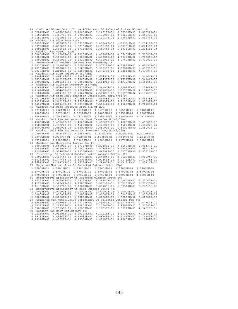
145
68 Combined Blower/Motor/Drive Efficiency Of Selected Indoor Blower (%) 3.52072E+01 3.41903E+01 3.29636E+01 3.14011E+01 3.00588E+01 2.87032E+01 3.51855E+01 3.41575E+01 3.29075E+01 3.13590E+01 3.00286E+01 2.86841E+01 3.51523E+01 3.41098E+01 3.28310E+01 3.13030E+01 2.99893E+01 2.86576E+01 69 Outdoor Air Flow Rate (cfm) 1.80982E+03 1.69069E+03 1.57156E+03 1.45244E+03 1.33331E+03 1.21418E+03 1.80982E+03 1.69069E+03 1.57156E+03 1.45244E+03 1.33331E+03 1.21418E+03 1.80982E+03 1.69069E+03 1.57156E+03 1.45244E+03 1.33331E+03 1.21418E+03 70 Outdoor Fan Speed (rpm) 5.53000E+02 5.16600E+02 4.80200E+02 4.43800E+02 4.07400E+02 3.71000E+02 5.53000E+02 5.16600E+02 4.80200E+02 4.43800E+02 4.07400E+02 3.71000E+02 5.53000E+02 5.16600E+02 4.80200E+02 4.43800E+02 4.07400E+02 3.71000E+02 71 Percentage Of Nominal Outdoor Fan Frequency (%) 6.70303E+01 6.26182E+01 5.82060E+01 5.37939E+01 4.93818E+01 4.49697E+01 6.70303E+01 6.26182E+01 5.82060E+01 5.37939E+01 4.93818E+01 4.49697E+01 6.70303E+01 6.26182E+01 5.82060E+01 5.37939E+01 4.93818E+01 4.49697E+01 72 Outdoor Air Face Velocity (ft/min) 1.99980E+02 1.86816E+02 1.73653E+02 1.60490E+02 1.47327E+02 1.34164E+02 1.99980E+02 1.86816E+02 1.73653E+02 1.60490E+02 1.47327E+02 1.34164E+02 1.99980E+02 1.86816E+02 1.73653E+02 1.60490E+02 1.47327E+02 1.34164E+02 73 Outdoor Air Surface Velocity (ft/min) 3.21616E+02 3.00446E+02 2.79277E+02 2.58107E+02 2.36937E+02 2.15768E+02 3.21616E+02 3.00446E+02 2.79277E+02 2.58107E+02 2.36937E+02 2.15768E+02 3.21616E+02 3.00446E+02 2.79277E+02 2.58107E+02 2.36937E+02 2.15768E+02 74 Outdoor Air-Side Heat Transfer Coefficient (Btu/h/ft2/F) 8.76709E+00 8.40844E+00 8.03981E+00 7.65958E+00 7.26841E+00 6.86478E+00 8.70135E+00 8.34511E+00 7.97908E+00 7.60258E+00 7.21500E+00 6.81509E+00 8.64127E+00 8.28743E+00 7.92388E+00 7.55044E+00 7.16607E+00 6.76987E+00 75 Outdoor Air-Side Pressure Drop (In Of H2O) 5.87446E–02 5.22247E–02 4.60349E–02 4.01795E–02 3.46544E–02 2.94661E–02 1.18865E–01 1.05761E–01 9.32996E–02 8.14870E–02 3.36568E–02 2.86096E–02 1.15640E–01 1.02893E–01 9.07717E–02 7.92681E–02 6.83920E–02 2.78116E–02 76 Outdoor Coil Fin Patternation Heat Transfer Multiplier 1.45000E+00 1.45000E+00 1.45000E+00 1.45000E+00 1.45000E+00 1.45000E+00 1.45000E+00 1.45000E+00 1.45000E+00 1.45000E+00 1.45000E+00 1.45000E+00 1.45000E+00 1.45000E+00 1.45000E+00 1.45000E+00 1.45000E+00 1.45000E+00 77 Outdoor Coil Fin Patternation Pressure Drop Multiplier 1.02962E+00 1.01449E+00 9.98597E–01 9.81952E–01 9.63252E–01 9.42008E–01 1.00735E+00 9.92773E–01 9.77275E–01 9.60453E–01 9.41497E–01 9.20002E–01 9.87129E–01 9.72867E–01 9.57699E–01 9.40830E–01 9.21763E–01 8.99878E–01 78 Outdoor Fan Operating Torque (oz-ft) 6.30075E+00 5.56590E+00 4.87387E+00 4.22481E+00 3.61823E+00 3.05437E+00 1.14560E+01 1.01991E+01 9.00501E+00 7.87388E+00 3.54560E+00 2.99110E+00 1.11390E+01 9.91460E+00 8.75164E+00 7.64894E+00 6.60708E+00 2.93315E+00 79 Percentage Of Selected Outdoor Motor Nominal Torque (%) 3.93996E+01 3.48044E+01 3.04771E+01 2.64184E+01 2.26254E+01 1.90994E+01 7.16361E+01 6.37766E+01 5.63098E+01 4.92366E+01 2.21712E+01 1.87038E+01 6.96542E+01 6.19976E+01 5.47254E+01 4.78300E+01 4.13151E+01 1.83414E+01 80 Required Nominal Size Of Selected Outdoor Motor (Hp) 1.57000E–01 1.57000E–01 1.57000E–01 1.57000E–01 1.57000E–01 1.57000E–01 1.57000E–01 1.57000E–01 1.57000E–01 1.57000E–01 1.57000E–01 1.57000E–01 1.57000E–01 1.57000E–01 1.57000E–01 1.57000E–01 1.57000E–01 1.57000E–01 81 Motor/Drive Efficiency Of Selected Outdoor Drive (%) 7.16252E+01 6.91693E+01 6.59773E+01 6.29887E+01 6.02802E+01 5.75060E+01 7.41266E+01 7.32542E+01 7.18807E+01 7.08031E+01 6.00360E+01 5.73119E+01 7.41484E+01 7.31971E+01 7.17668E+01 7.07789E+01 6.88519E+01 5.71341E+01 82 Motor/Drive Efficiency Of Base Outdoor Drive (%) 1.00000E+02 1.00000E+02 1.00000E+02 1.00000E+02 1.00000E+02 1.00000E+02 1.00000E+02 1.00000E+02 1.00000E+02 1.00000E+02 1.00000E+02 1.00000E+02 1.00000E+02 1.00000E+02 1.00000E+02 1.00000E+02 1.00000E+02 1.00000E+02 83 Combined Fan/Motor/Drive Efficiency Of Selected Outdoor Fan (%) 2.89449E+01 2.81309E+01 2.70108E+01 2.59651E+01 2.50245E+01 2.40461E+01 3.33371E+01 3.29250E+01 3.22803E+01 3.17601E+01 2.47016E+01 2.37605E+01 3.33650E+01 3.29256E+01 3.22637E+01 3.17930E+01 3.08917E+01 2.34811E+01 84 Outdoor Fan-Only Efficiency (%) 4.04116E+01 4.06696E+01 4.09396E+01 4.12218E+01 4.15137E+01 4.18149E+01 4.49732E+01 4.49462E+01 4.49082E+01 4.48569E+01 4.11447E+01 4.14582E+01 4.49976E+01 4.49821E+01 4.49564E+01 4.49187E+01 4.48669E+01 4.10982E+01

146
85 Outdoor Fan Specific Speed 1.97159E+05 1.94437E+05 1.91545E+05 1.88466E+05 1.85211E+05 1.81771E+05 1.16212E+05 1.14536E+05 1.12766E+05 1.10897E+05 1.89313E+05 1.85836E+05 1.18635E+05 1.16922E+05 1.15113E+05 1.13217E+05 1.11232E+05 1.89821E+05 86 Required Refrigerant Charge (lbm) 7.50985E+00 7.35836E+00 7.17066E+00 6.96274E+00 6.91199E+00 7.33606E+00 7.30869E+00 7.15395E+00 7.00757E+00 6.89639E+00 6.85434E+00 7.02440E+00 7.47282E+00 7.33289E+00 7.20861E+00 7.12385E+00 7.09869E+00 7.22922E+00 87 Required Capillary Flow Factor 1.21600E+00 1.07633E+00 9.39395E–01 8.21744E–01 6.39803E–01 3.85069E–01 1.70160E+00 1.53953E+00 1.37303E+00 1.18212E+00 9.33278E–01 6.24370E–01 2.22647E+00 2.04173E+00 1.85073E+00 1.59404E+00 1.26948E+00 8.91257E–01 88 Required TXV Capacity Rating (Tons) 6.52690E–01 5.73228E–01 5.02736E–01 4.44119E–01 3.57799E–01 2.42071E–01 9.17941E–01 8.24142E–01 7.32112E–01 6.33391E–01 5.13124E–01 3.68625E–01 1.23416E+00 1.11726E+00 1.00307E+00 8.65020E–01 7.05802E–01 5.30161E–01 89 Fraction Of Rated TXV Opening 1.00000E+00 1.00000E+00 1.00000E+00 1.00000E+00 1.00000E+00 1.00000E+00 1.00000E+00 1.00000E+00 1.00000E+00 1.00000E+00 1.00000E+00 1.00000E+00 1.00000E+00 1.00000E+00 1.00000E+00 1.00000E+00 1.00000E+00 1.00000E+00 90 Required Short Tube Orifice Diameter (In) 3.53549E–02 3.31155E–02 3.08688E–02 2.88252E–02 2.59381E–02 2.06967E–02 4.28018E–02 4.06544E–02 3.83227E–02 3.54764E–02 3.14364E–02 2.55628E–02 5.02921E–02 4.80838E–02 4.56756E–02 4.22660E–02 3.76798E–02 3.16748E–02 91 Required Simple Orifice Effective KA Product (In2) 6.19236E–04 5.45346E–04 4.79289E–04 4.24049E–04 3.42261E–04 2.31951E–04 8.63958E–04 7.78723E–04 6.94135E–04 6.02487E–04 4.89690E–04 3.52787E–04 1.14839E–03 1.04565E–03 9.43637E–04 8.18356E–04 6.71279E–04 5.06409E–04 92 Evaporator Exit Refrigerant Superheat (F) Or Quality (–) –9.94918E–01 –9.93846E–01 –9.92568E–01 –9.91164E–01 –9.88259E–01 –9.81177E–01 –9.96792E–01 –9.96136E–01 –9.95254E–01 –9.94095E–01 –9.91847E–01 –9.87365E–01 –9.98036E–01 –9.97576E–01 –9.97055E–01 –9.95913E–01 –9.94326E–01 –9.90960E–01 93 Compressor Inlet Refrigerant Superheat (F) Or Quality (–) 1.00000E+00 1.00000E+00 1.00000E+00 1.00000E+00 1.00000E+00 1.00000E+00 1.00000E+00 1.00000E+00 1.00000E+00 1.00000E+00 1.00000E+00 1.00000E+00 1.00000E+00 1.00000E+00 1.00000E+00 1.00000E+00 1.00000E+00 1.00000E+00 94 Compressor Exit Refrigerant Superheat (F) Or Quality (–) 9.28456E+01 8.66525E+01 8.09977E+01 6.95736E+01 6.26807E+01 6.74081E+01 7.96038E+01 7.47014E+01 6.78053E+01 5.79722E+01 5.10873E+01 4.83998E+01 7.22503E+01 6.82708E+01 6.05123E+01 5.12229E+01 4.41918E+01 3.81429E+01 95 Condenser Exit Refrigerant Subcooling (F) Or Quality (–) 2.40163E+01 2.12248E+01 1.84009E+01 1.56017E+01 1.28011E+01 1.00077E+01 2.40206E+01 2.12044E+01 1.84000E+01 1.56053E+01 1.27939E+01 1.00085E+01 2.39942E+01 2.12010E+01 1.84050E+01 1.55967E+01 1.28134E+01 9.99316E+00 96 Flow Control Inlet Refrigerant Subcooling (F) Or Quality (–) 3.85271E+01 3.81667E+01 3.83289E+01 3.88500E+01 4.27128E+01 5.62174E+01 3.38741E+01 3.26723E+01 3.18529E+01 3.18533E+01 3.38842E+01 4.11991E+01 3.06879E+01 2.91100E+01 2.77840E+01 2.72814E+01 2.83031E+01 3.25375E+01 97 Refrigerant Temperature At Flow Control Inlet (F) 5.76814E+01 5.51873E+01 5.22573E+01 4.91361E+01 4.20865E+01 2.46884E+01 6.74846E+01 6.58362E+01 6.37567E+01 6.04868E+01 5.45868E+01 4.26087E+01 7.75333E+01 7.61461E+01 7.42104E+01 7.05335E+01 6.46754E+01 5.48985E+01 98 Refrigerant Suction Temperature At Compressor Inlet (F) 9.48881E+00 1.02611E+01 1.09429E+01 1.16559E+01 1.24196E+01 1.34561E+01 2.21796E+01 2.29095E+01 2.36031E+01 2.43723E+01 2.55040E+01 2.70074E+01 3.45797E+01 3.53631E+01 3.61113E+01 3.70616E+01 3.83258E+01 4.01378E+01 99 Refrigerant Discharge Temperature At Compressor Exit (F) 1.89600E+02 1.80445E+02 1.71932E+02 1.57839E+02 1.47671E+02 1.48409E+02 1.81906E+02 1.73986E+02 1.64042E+02 1.50793E+02 1.39888E+02 1.32372E+02 1.81940E+02 1.74752E+02 1.63507E+02 1.49794E+02 1.37683E+02 1.25877E+02 100 Refrigerant Suction Pressure At Compressor Inlet (psia) 4.60435E+01 4.67660E+01 4.74104E+01 4.80901E+01 4.88288E+01 4.98450E+01 5.90421E+01 5.98642E+01 6.06562E+01 6.15417E+01 6.28641E+01 6.46526E+01 7.42568E+01 7.53082E+01 7.63236E+01 7.76244E+01 7.93839E+01 8.19598E+01 101 Refrigerant Discharge Pressure At Compressor Exit (psia) 2.01361E+02 1.93195E+02 1.85546E+02 1.78606E+02 1.70355E+02 1.60686E+02 2.17343E+02 2.08540E+02 1.99919E+02 1.90566E+02 1.79980E+02 1.67852E+02 2.40050E+02 2.29983E+02 2.19407E+02 2.06492E+02 1.92379E+02 1.77244E+02

147
102 Required Indoor Duct Size (Inches) 6.22000E+00 6.22000E+00 6.22000E+00 6.22000E+00 6.22000E+00 6.22000E+00 6.22000E+00 6.22000E+00 6.22000E+00 6.22000E+00 6.22000E+00 6.22000E+00 6.22000E+00 6.22000E+00 6.22000E+00 6.22000E+00 6.22000E+00 6.22000E+00 103 Indoor Duct Pressure Drop (Inches of Water) 1.13635E–01 1.01056E–01 8.91031E–02 7.77764E–02 6.71618E–02 5.72620E–02 1.13004E–01 1.00482E–01 8.85949E–02 7.73830E–02 6.68748E–02 5.70785E–02 1.12076E–01 9.96637E–02 8.79012E–02 7.68597E–02 6.65021E–02 5.68237E–02 104 Indoor Filter Pressure Drop (Inches of Water) 5.30885E–02 4.67183E–02 4.07315E–02 3.51262E–02 2.99378E–02 2.51635E–02 5.27938E–02 4.64529E–02 4.04992E–02 3.49485E–02 2.98099E–02 2.50829E–02 5.23602E–02 4.60744E–02 4.01821E–02 3.47121E–02 2.96437E–02 2.49709E–02 105 Indoor Heater Pressure Drop (Inches of Water) 7.62020E–02 6.70585E–02 5.84651E–02 5.04193E–02 4.29720E–02 3.61192E–02 7.57790E–02 6.66775E–02 5.81317E–02 5.01643E–02 4.27884E–02 3.60034E–02 7.51567E–02 6.61343E–02 5.76765E–02 4.98250E–02 4.25499E–02 3.58427E–02 106 Indoor Coil Pressure Drop (Inches of Water) 6.91029E–02 6.18728E–02 5.49590E–02 4.83635E–02 4.21319E–02 3.62685E–02 6.87890E–02 6.15836E–02 5.46998E–02 4.81601E–02 4.19813E–02 3.61706E–02 6.83279E–02 6.11719E–02 5.43464E–02 4.78897E–02 4.17858E–02 3.60348E–02 107 Selected Compressor–Only Isentropic Efficiency — Excluding Motor (%) 5.68977E+01 5.75967E+01 5.79781E+01 6.26377E+01 6.49033E+01 6.03007E+01 5.97086E+01 6.02815E+01 6.20312E+01 6.59214E+01 6.82646E+01 6.74002E+01 6.10114E+01 6.12838E+01 6.36784E+01 6.72649E+01 6.95707E+01 7.08615E+01 108 Baseline Compressor-Only Isentropic Efficiency — Excluding Motor (%) 5.62622E+01 5.77164E+01 5.84405E+01 6.31776E+01 6.53625E+01 6.02560E+01 5.86510E+01 6.00114E+01 6.22781E+01 6.61910E+01 6.86569E+01 6.72627E+01 5.95264E+01 6.07337E+01 6.37356E+01 6.73611E+01 6.98819E+01 7.07092E+01 109 Wetted Fraction of Evaporator Coil 0.00000E+00 0.00000E+00 0.00000E+00 0.00000E+00 0.00000E+00 0.00000E+00 6.74810E–01 5.79088E–01 4.50076E–01 2.08695E–01 0.00000E+00 0.00000E+00 7.86742E–01 7.24058E–01 6.44594E–01 4.79373E–01 1.54217E–02 0.00000E+00 110 Moisture Removal Rate (lbm/h) 0.00000E+00 0.00000E+00 0.00000E+00 0.00000E+00 0.00000E+00 0.00000E+00 3.61055E–01 2.40540E–01 1.33662E–01 3.64602E–02 0.00000E+00 0.00000E+00 8.20077E–01 6.22692E–01 4.38385E–01 2.09952E–01 2.02284E–04 0.00000E+00


149
APPENDIX D
DEFINITIONS OF CONSTANTS ASSIGNED IN BLOCK DATA
A number of variables and constants are used by the Heat Pump Design Model that are unlikely tobe changed very often, and consequently they are simply assigned values rather than being specifiedwith each set of input data. They have been brought together in the BLOCK DATA subroutine andgiven values which are in turn passed to the subroutines where they are used via common blocks.These data are divided into several categories organized by function.
Assignment of Unit Numbers for Input and Output
Input Unit Numbers
IOCHZR for reading ‘CONCHZ’ and ‘HPDATA’ data files, 5
IOCNTR for reading ‘CONTRL’ data files (optional), 24
Output Unit Numbers
IOCONW for printing the input echo and the output listing, 6
IOSSP for punching a steady-state performance data file of the form required for the ORNLAnnual Performance Factor Model, 7
IOCONP for punching contour data files ‘CONGEN’ or ‘CONSPD’ (from Figure CDG1), 8
Physical Air-Side Parameters
PA atmospheric pressure, 14.7 lbf/in.2
RAU universal gas constant, 53.34 ft-lbf/lbm-�R
AFILTR flow area of filter on indoor unit, 2.78 ft2
AHEATR cross-sectional area of resistance heater section in indoor unit, (usually equal toindoor blower exit area), 1.28 ft2
RACKS number of resistance heater racks, 3.0
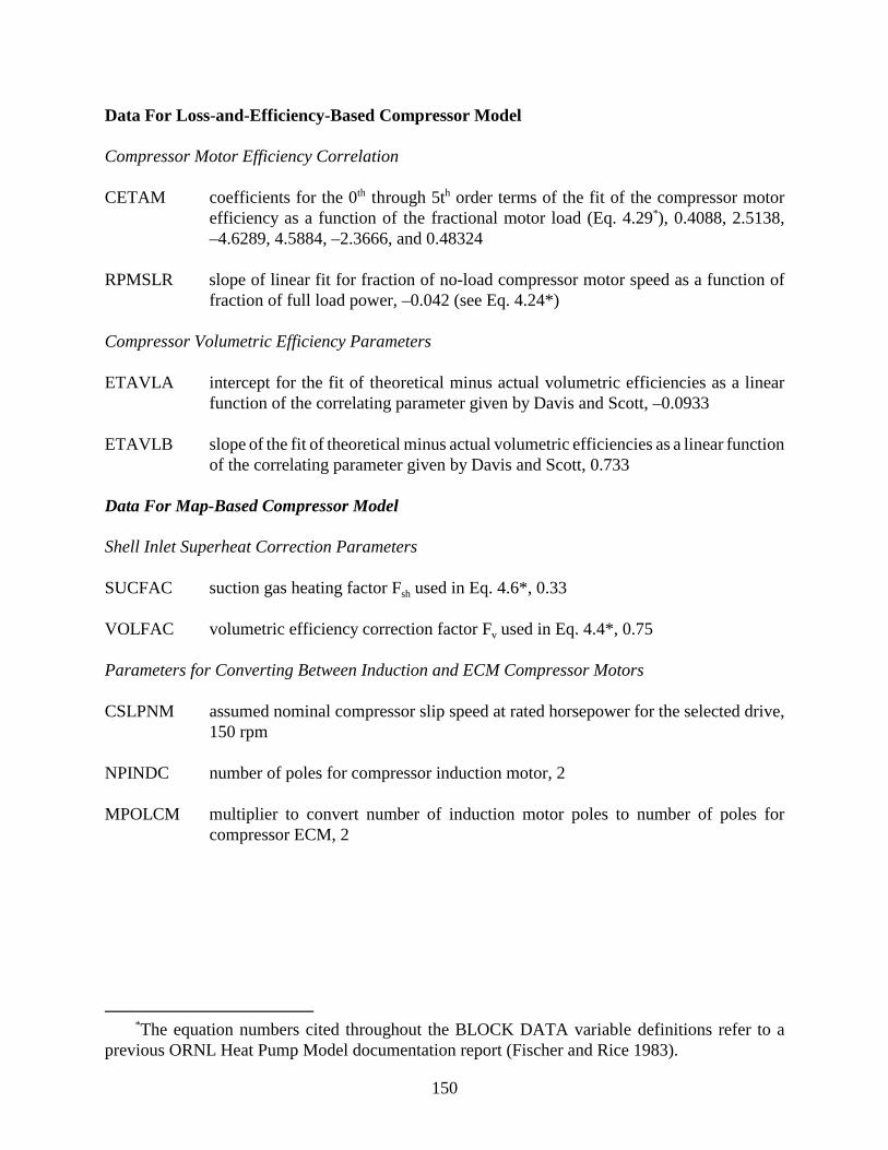
*The equation numbers cited throughout the BLOCK DATA variable definitions refer to aprevious ORNL Heat Pump Model documentation report (Fischer and Rice 1983).
150
Data For Loss-and-Efficiency-Based Compressor Model
Compressor Motor Efficiency Correlation
CETAM coefficients for the 0th through 5th order terms of the fit of the compressor motorefficiency as a function of the fractional motor load (Eq. 4.29*), 0.4088, 2.5138,–4.6289, 4.5884, –2.3666, and 0.48324
RPMSLR slope of linear fit for fraction of no-load compressor motor speed as a function offraction of full load power, –0.042 (see Eq. 4.24*)
Compressor Volumetric Efficiency Parameters
ETAVLA intercept for the fit of theoretical minus actual volumetric efficiencies as a linearfunction of the correlating parameter given by Davis and Scott, –0.0933
ETAVLB slope of the fit of theoretical minus actual volumetric efficiencies as a linear functionof the correlating parameter given by Davis and Scott, 0.733
Data For Map-Based Compressor Model
Shell Inlet Superheat Correction Parameters
SUCFAC suction gas heating factor Fsh used in Eq. 4.6*, 0.33
VOLFAC volumetric efficiency correction factor Fv used in Eq. 4.4*, 0.75
Parameters for Converting Between Induction and ECM Compressor Motors
CSLPNM assumed nominal compressor slip speed at rated horsepower for the selected drive,150 rpm
NPINDC number of poles for compressor induction motor, 2
MPOLCM multiplier to convert number of induction motor poles to number of poles forcompressor ECM, 2

151
Factors For Estimating Suction Gas Superheat Effects Of Different Motors
LOCOOL logical variable used to omit suction gas superheat corrections if motor is not low-side cooled, .TRUE.
HTFRAC estimated fraction of the shaft input power (heat from non-motor sources) thatcontributes to suction gas heating, 0.05
DAMPER damping factor on total suction gas heating from motor cooling and from heattransfer from the compressor body and discharge line, 0.75
PM-ECM Motor Characteristics (Used for Motor Temperature Corrections)
ETSTAT estimate of motor stator temperature, 40.0 �C
ETROTR estimate of motor rotor temperature, 55.0 �C
ETREF reference temperature for motor data, 25.0 �C
ETCOEF magnet flux temperature coefficient (–0.20% / �C)
EFORMF approximate average form factor, 1.01
ESPDNM(J) motor nominal speed (rpm), 5400., 6900.
ETQRAT(J) rating point (design cooling load) torque (oz-ft), 64.0, 50.0
ERTREF(J) motor stator resistance (line-line) at reference temperature (ohms), 0.648, 0.371
EACOEF(J) slope of torque / current relationship, 0.205, 0.263
EBCOEF(J) intercept of torque / current relationship, 0.6, 0.3where ( I = A * T + B ) for two motor speeds J = 1,2 which provide 2 points from which to interpolate to other nominal speeds
Fan and Fan Motor Parameters
Data for Outdoor Fan Efficiency Representation
COFAN constant term for the fit of outdoor fan static efficiency to fan specific speed, –3.993
ClFAN coefficient for the linear term of the fit of outdoor fan static efficiency to the fanspecific speed, 4.266
C2FAN coefficient for the quadratic term of the fit of outdoor fan static efficiency to fanspecific speed, –1.024

152
Fan Power Reference Temperatures
TRFIDF(1) reference temperature for indoor fan power in cooling mode, 80.0�F
TRFIDF(2) reference temperature for indoor fan power in heating mode, 70.0�F
TRFODF(1) reference temperature for outdoor fan power in cooling mode, 95.0�F
TRFODF(2) reference temperature for outdoor fan power in heating mode, 47.0�F
Parameters for Converting Between Induction and ECM Fan Motors
SLPNMI indoor-blower assumed nominal slip speed at rated horsepower, 120 rpm
SLPNMI outdoor-fan assumed nominal slip speed at rated horsepower, 120 rpm
NPOLEI number of poles for indoor-blower induction motor, 6
NPOLEO number of poles for outdoor-fan induction motor, 6
MPOLEI multiplier to convert number of induction motor poles to number of poles for indoor-blower ECM, 2
MPOLEO multiplier to convert number of induction motor poles to number of poles foroutdoor-fan ECM, 2
Iteration Convergence Criteria (Default Values)
AMBCON Convergence parameter for the iteration on evaporator inlet air temperature, 0.20�F
CNDCON Convergence parameter for the iteration on condenser exit subcooling(or on exitquality * 200) — used when IREFC = 0 on Line 6 (F�); also the quantity {2 *CNDCON} is used as the convergence parameter for the charge balancing iterationwhen ICHRGE =2, 0.20�F
FLOCON Convergence parameter for iteration on refrigerant mass flow rate — used whenIREFC › 0 on Line 6 (equivalent F�) value is specified as if it were in degrees F andis scaled internally (by 1/20th) to give a mass flow convergence factor, 0.20 F�
EVPCON Convergence parameter for iteration on evaporator exit superheat (or on exit quality* 500); Also the quantity {2 * EVPCON} is used as the convergence parameter forthe charge balancing iteration when ICHRGE =1, 0.50 F�
CONMST Convergence parameter for iterations on evaporator tube wall temperatures insubroutine EVAP and dew-point temperature in subroutine XMOIST, 0.003 F�

153
Iteration Convergence Criteria (continued)
CMPCON Convergence parameter for iteration on suction gas enthalpy in the efficiency-and-loss compressor model (Btu/lbm) — only used when ICOMP = 1 on Line 8, 0.05 F�
TOLH Tolerance parameter used by refrigerant routines in calculating properties ofsuperheated vapor when converging on a known enthalpy value (Btu/lbm), 0.001
TOLS Tolerance parameter used by refrigerant routines in calculating properties ofsuperheated vapor when converging on a known entropy value (Btu/lbm/�R),0.00005
Refrigerant Specification (Default)
NR refrigerant number, 22
Refrigerant-Side Heat Transfer Correlation for Condenser Vapor Region
ClR, C3R, and C5R coefficients for single-phase heat transfer coefficient(Eq. 6.2*), 1.10647, 3.5194 × 10⁻⁷, and 0.01080
C2R, C4R, and C6Rexponents for single-phase heat transfer coefficient (Eq. 6.3*), –0.78992, 1.03804, and –0.13750
XLLR lower limit on the Reynolds number for laminar flow of refrigerant, 3,500
ULR upper limit for the Reynolds number for turbulent flow of refrigerant, 6,000
Refrigerant Tubing Parameter
E roughness of interior tube walls, 5 × 10⁻⁶ ft
Evaporator Dryout Criterion
XDO refrigerant quality at which dryout occurs in the evaporator, 0.75

154
Refrigerant Flow Control Parameters
Thermostatic Expansion Valve Constants (Set for R22 as Default)
BLEEDF bypass or bleed factor coefficient used to compute TXV parameters when condensersubcooling is held fixed, 1.15
DPRAT rated pressure drop across the TXV at the design conditions, 100 psi for R-22 andR-502, 60 psi for R-12
NZTBOP switch to bypass nozzle and distributor tube pressure drop calculations whencalculating TXV parameters if the condenser subcooling is held fixed, 0
STATIC static superheat setting used to compute the TXV parameters when the condensersubcooling is held fixed, 6.0 F�
SUPRAT rated operating superheat used to compute the TXV parameters when the condensersubcooling is held fixed, 11.0 F�
TERAT rated evaporating temperature for the TXV, 40.0�F
TLQRAT rated liquid refrigerant temperature at the inlet to the TXV, 100.0�F
XLTUBE length of distributor tubes (if used), 30 inches
Capillary Tube Parameter
NCAP number of capillary tubes used to compute capillary tube flow factor, , whencondenser subcooling is held fixed, 1

155
APPENDIX E
DESCRIPTION OF NEW SUBROUTINES ADDEDSINCE THE MARK III VERSION
New Compressor-Drive-Performance Routines — Inverter- and Sine-Wave-Driven Induction Motors (IDIM and SWDIMs) and Permanent-Magnet-Electronically-Commutated-Motors (PM-ECMs)
(in general order of increasing drive efficiency)
CMPFGN computes efficiency reduction factor for first generation inverter drives compared topure sine wave performance at the same frequency — function of compressorfrequency (15 to 90 Hz) and operation mode (heating or cooling) — integral Hp size
CMPSOA computes efficiency reduction factor for state-of-the-art inverter drives compared topure sine wave performance at the same frequency — function of compressorfrequency (15 to 90 Hz) and operation mode (heating or cooling) — integral Hp size
SWDIM interpolates the motor efficiency and speed of a variable-frequency, 2-pole hermetic,sine-wave-driven induction motor (SWDIM) as a function of fractional full load (0.2to 2.0), frequency ratio (0.25 to 1.5), and Volts/Hz multiplier (0.9 to 1.1) — integralHp size
ITRIND iterates to find sine-wave-driven induction motor efficiency and speed givenelectrical input power and drive frequency
ITRECM iterates to find PM-ECM motor efficiency given electrical input power and drivespeed
ECMCMP interpolates the combined drive/motor efficiency of a variable-frequency compressorPM-ECM (4-pole hermetic) as a function of fractional full load (0.2 to 1.9 of fullload) and drive frequency ratio (0.2 to 1.15 of nominal) — integral Hp size
ECMTMP corrects ECM motor efficiency for hermetic operating temperature effects as afunction of fractional rated torque and operating speed ratio
PROPCM computes refrigerant property values needed to convert compressor-map isentropicand volumetric efficiency values to power and mass flow rate, respectively
New Fan-Drive-Performance Routines — Inverter- and Sine-Wave-Driven Induction Motors (IDIM and SWDIMs) and Permanent-Magnet-Electronically-Commutated-Motors (PM-ECMs)
(in general order of increasing drive efficiency)

156
New Fan-Drive-Performance Routines — (continued)
FANFGN computes modulating blower combined-motor-and-drive efficiency for a firstgeneration inverter-driven system (fractional Hp size)
FANSOA computes modulating blower combined-motor-and-drive efficiency for a state-of-the-art inverter-driven system (fractional Hp size)
FANSWV computes modulating blower combined-motor-and-drive efficiency for a sine-wave-driven system (fractional Hp size)
ECMBLW interpolates the combined drive/motor efficiency of a variable-frequency blower PM-ECM (12-pole) as a function of fractional full load (0.2 to 1.6 of full load) and drivespeed (300 to 1300 rpm)
ECMTRQ routine to calculate PM-ECM fan drive efficiency as a function of drive speed andair-side pressure drop (similar in function to ITRIND AND ITRECM for thecompressor except that iteration is not required because blower torque is calculateddirectly from first principles rather than derived from required power input in thecase of the compressor); also calculates required motor size if user-requested
Refrigerant-Charge-Inventory-Related Routines
(in order of occurrence in structure diagram of heat pump model)
General Charge Inventory Computations
INVENT calculates total low- and high-side refrigerant mass at steady-state and equilibrium(off-cycle) conditions, prints summary of refrigerant mass in each component
ZEROCH root-finding routine for the charge balancing outermost iteration loop of the heatpump model
GUESS1 routine which determines two values of evaporator superheat (or condensersubcooling) which require refrigerant charges that bracket the required charge
CHARGM function routine called by ZEROCH and GUESS1 which in turn calls the heat pumpmodel subroutine HPDM and calculates and prints, as required, the difference inrefrigerant charge between the calculated and the specified values
ACCUML calculates refrigerant liquid level and mass in a suction line accumulator —accommodates j-tube holes at two user-specified heights
HXCHRG general purpose routine to calculate refrigerant mass in single and two-phase sectionsof a tube-and-fin heat exchanger
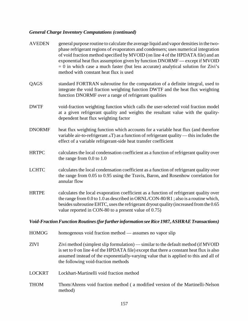
157
General Charge Inventory Computations (continued)
AVEDEN general purpose routine to calculate the average liquid and vapor densities in the two-phase refrigerant regions of evaporators and condensers; uses numerical integrationof void fraction method specified by MVOID (on line 4 of the HPDATA file) and anexponential heat flux assumption given by function DNORMF — except if MVOID= 0 in which case a much faster (but less accurate) analytical solution for Zivi’smethod with constant heat flux is used
QAGS standard FORTRAN subroutine for the computation of a definite integral, used tointegrate the void fraction weighting function DWTF and the heat flux weightingfunction DNORMF over a range of refrigerant qualities
DWTF void-fraction weighting function which calls the user-selected void fraction modelat a given refrigerant quality and weights the resultant value with the quality-dependent heat flux weighting factor
DNORMF heat flux weighting function which accounts for a variable heat flux (and thereforevariable air-to-refrigerant �T) as a function of refrigerant quality — this includes theeffect of a variable refrigerant-side heat transfer coefficient
HRTPC calculates the local condensation coefficient as a function of refrigerant quality overthe range from 0.0 to 1.0
LCHTC calculates the local condensation coefficient as a function of refrigerant quality overthe range from 0.05 to 0.95 using the Travis, Baron, and Rosenhow correlation forannular flow
HRTPE calculates the local evaporation coefficient as a function of refrigerant quality overthe range from 0.0 to 1.0 as described in ORNL/CON-80/R1 ; also is a routine which,besides subroutine EHTC, uses the refrigerant dryout quality (increased from the 0.65value reported in CON-80 to a present value of 0.75)
Void-Fraction Function Routines (for further information see Rice 1987, ASHRAE Transactions)
HOMOG homogenous void fraction method — assumes no vapor slip
ZIVI Zivi method (simplest slip formulation) — similar to the default method (if MVOIDis set to 0 on line 4 of the HPDATA file) except that there a constant heat flux is alsoassumed instead of the exponentially-varying value that is applied to this and all ofthe following void-fraction methods
LOCKRT Lockhart-Martinelli void fraction method
THOM Thom/Ahrens void fraction method ( a modified version of the Martinelli-Nelsonmethod)

158
Void-Fraction Function Routines (for further information see Rice 1987, ASHRAE Transactions)(continued)
BARCZY Baroczy void fraction method
PREMOL Premoli void fraction method (mass-flux dependent), only configured at present forR22 — needs surface tension properties for use with other refrigerants)
TANDON Tandon void fraction method (mass-flux dependent)
HUGHMK Hughmark void fraction method (mass-flux dependent)
ZEROZM zero-finding routine for internal iterations required in Hughmark void fractionmethod
ZMATCH computes the functional values of the Hughmark void fraction method based on built-in tables
Air-Side Heat-Transfer and Pressure-Drop Correlations
Air-Side Heat Transfer
ZIGHTM calculates augmentation factor for the air-side heat transfer coefficient due to finpatternation with specific zig-zag fin designs
NUAFF used in function ZIGHTM to correct a Nussult number ratio as a function of finspacing and Graetz number
SINTRP interpolation in a single independent variable using a three point lagrangian method(for use with function ZIGHTM)
Air-Side Pressure Drop
KLOSS calculates contraction and expansion losses entering and leaving a finned heatexchanger (based on Kays and London correlations)
ZIGPDM calculates a multiplying factor for air pressure drop of specific zig-zag fin surfacesrelative to an unpatterned fin
Front-End Routines For Contour Data Generation
CONDRV main program and first-level driving routine, reads CONCHZ input data file directlyand calls DATAIN to read HPDATA file, also calls CONDAT to punch generalcontour data files

159
Front-End Routines For Contour Data Generation (continued)
APFDRV second-level driver routine, reads ambient / speed / control data file ‘CONTRL’ andperforms selected and dual-mode ambient-vs-speed performance mapping, can punchdata file of the form required for the ORNL Annual Performance Factor Model; cangenerate contour data sets for selected indoor and outdoor ambients and relativehumidities whereas with CONCHZ users can only select ambients with a uniformgrid and fixed relative humidity
SSDRV third-level driver routine controlling the individual calls to the ORNL ModulatingHeat Pump Design Model
DATAIN modified version of original DATAIN which is now called from CONDRV anddefers assignment of input values for the condenser and the evaporator to subroutineHX
HX converts indoor and outdoor heat exchanger data from input file HPDATA intocondenser and evaporator values
TRNVAL assigns contour grid values of independent variables (defined in Table XXX)specified in CONCHZ to the appropriate program variables and performs anynecessary adjustment of related parameters (such as to maintain a constant total heatexchanger area)
NEWVAL routine that provides user-specified operational control of design variables as afunction of either outdoor ambient temperature or compressor frequency
DPVLSS saves values of steady-state dependent parameters (defined in Table YYY) computedby the heat pump model — in arrays suitable for use by CONDAT in selecting whichare to be punched in output data sets
APF (presently not included) calculates annual performance factor (APF) for set of speedversus ambient data generated by APFDRV
DPVAPF (presently not used) saves values of seasonal performance variables computed by theORNL Annual Performance Factor Model — in arrays suitable for use by CONDATin selecting which are to be punched in output data sets
CONDAT generalized routine for punching contour data sets of parameters that have been user-selected in input data set CONCHZ

160
All Input/Output Data Files and Default Unit Numbers (Set in BLOCK DATA )
(as identified on structure diagram of MODCON program)
Input* Unit Numbers Purpose
CONCHZ 5 Contour Selection Data File
HPDATA 5 Heat Pump Specification Data File
CONTRL 24 (optional) Ambient / Speed / Control Data File For Selected and Dual-Mode Ambient-Vs-Speed Performance Mapping
Output Unit Numbers Purpose
PRINT 6 Program Input Echo and Output Listing of Type Selected in Data File HPDATA
APFSS 7 (optional) Steady-State Performance Data File of the Form Requiredfor the ORNL Annual Performance Factor Model
CONGEN 8 Contour Data Generation File of the Independent andDependent Variables Selected in Data File CONCHZ
CONSPD 8 (optional) Contour Data Generation File of the Independent andDependent Variables Selected in Data File CONTRL
APFDYN not yet in use Dynamic Loss Data Needed along with Data File APFSSto run the ORNL Annual Performance Factor Model
____________ *The order of input data file calls is CONCHZ, HPDATA, then CONTRL. However, design andoperating parameters set initially in HPDATA, if selected as parametric variables, are overridden incalls to routine TRNVAL, defined by the selected parametric inputs set in CONCHZ, and optionallyby calls to input data file CONTRL from routine APFDRV.

161
APPENDIX F
DESCRIPTION OF SUBROUTINES USED FOR THEBASIC ORNL HEAT PUMP MODEL
HPDM original main program which serves as driving program for high- and low-sidecomputations and contains iterative loop converging on evaporator inlet airtemperature
BLOCK DATA assigns default values, values to constants, and infrequently changed parameters
CALC calculates geometric constants for both heat exchangers
CAPTUB refrigerant flow control model for capillary tube flow rate or sizing
CHTC calculates refrigerant-side heat transfer coefficient for the two-phase region of thecondenser
CMPMAP computes refrigerant mass flow and compressor power consumption fromcompressor map data
CNDNSR serves as driving routine for COMP, COND and FLOBAL and returns thedifference between the calculated and specified condenser subcooling or betweenthe compressor and expansion device refrigerant mass flow rates
COMP computes refrigerant mass flow rate and compressor power consumption fromefficiency and loss parameters
COND calculates total condenser heat transfer rate, air and refrigerant properties andrefrigerant and air-side pressure drops for fixed inlet refrigerant conditions
DPF determines an approximate dew-point temperature for a given vapor pressure ofmoist air
DPFSOL calculates the difference between the known saturation pressure of water vaporat the tube wall and the saturation pressure corresponding to an estimated, orgiven tube wall temperature
DPLINE determines the single-phase pressure drop in the refrigerant lines
EFFCT computes the difference in condenser effectiveness values between the generaleffectiveness equation and the specific cross-flow effectiveness equation as afunction of the fraction of the coil, fv, containing superheated refrigerant vapor

162
EHTC calculates refrigerant-side heat transfer coefficient for the two-phase region of theevaporator
EVAP determines the heat transfer, moisture removal, outlet air temperatures andhumidities from one circuit of the evaporator for given heat transfer coefficientsand saturation temperatures at the beginning and end of the two-phase region
EVAPR calculates evaporator heat transfer rate, air and refrigerant properties, andrefrigerant and air-side pressure drops for fixed exit refrigerant conditions
EVPTR serves as a driving routine for EVAPR and returns the difference between thespecified evaporator superheat and the calculated value
EXCH determines the heat transfer and outlet temperatures for one circuit of thecondenser for given heat transfer coefficients and saturation temperatures at thebeginning and end of the two-phase region
EXF determines the effectiveness of a cross-flow heat exchanger using theeffectiveness — NTU method
FANFIT calculates combined fan-fan motor efficiency given air-side pressure drop andvolumetric air-flow rate
FLOBAL determines refrigerant conditions at the inlet to the flow control device and drivesthe expansion device models
FRICT computes the general Moody friction factor for single phase flow in tubes
GUESS2 brackets a solution prior to using a root finder by shifting end points by factorsof 10
GUESS3 brackets a solution prior to using a root finder by shifting end points by constantstep
INTER interpolate in a single dimension using Lagrangian polynomial
HAIR computes air-side heat transfer coefficient for smooth fin and tube geometry
MUKCP calculates viscosity, thermal conductivity, and specific heat of 14 refrigerants
MUKCPA calculates viscosity, thermal conductivity, and specific heat of air
ORIFIC refrigerant flow control model for computing the refrigerant mass flow rate orsizing of a short-tube orifice
OUTPUT prints a detailed summary of output data

163
PDAIR calculates air-side pressure drop for smooth, wavy, or louvered fin-and-tube heatexchangers
PDROP determines single- and two-phase pressure drops for flow in heat exchanger tubes
PVSF calculates partial pressure of water vapor in saturated air
SATPRP evaluates the saturation thermodynamic properties of a specified refrigerant
SEFF determines surface efficiency for a hexagonal shaped fin surface
SLAG computes single-precision Lagrangian interpolation in two dimensions fromtabulated data
SPFHT calculates refrigerant specific heats at constant pressure and volume and specificheat ratio
SPHTC computes single-phase heat transfer coefficient for laminar, transition, orturbulent gas flow from an abrupt contraction entrance
SPHTC2 computes single-phase heat transfer coefficient for fully developed liquid or gasflow
SPVOL evaluates specific volume of superheated refrigerant
SUPCOR calculates power and mass flow correction factors for map-based compressormodel to correct for superheat level
TABLES assigns constants for selected refrigerant for use in the thermodynamic propertysubroutines
TAOSOL computes the exit air temperature from the region of the evaporator wheremoisture removal occurs
TRIAL determines thermodynamic properties of superheated refrigerant vapor given twoknown properties
TSAT calculates saturation temperature of refrigerant given saturation pressure
TWISOL used to compute the wall temperature at which moisture removal begins on theleading edge of the evaporator
TWOSOL used to compute the wall temperature at the exit from the evaporator
TXV refrigerant flow control model for computing the refrigerant mass flow rate orsizing for a thermostatic expansion valve

164
VAPOR determines thermodynamic properties of superheated refrigerant vapor giventemperature and pressure
WBF determines wet-bulb temperature of moist air
WTSFIT computes coefficients for a quadratic fit of wall temperature to enthalpy of moistair
XMOIST calculates dew point temperature, humidity ratio enthalpy, and wet-bulbtemperature or relative humidity of moist air
ZERO’s each of these routines solves for the root, or zero, of a function from two pointswhich bracket the solution using bisection and Newton’s method

165
APPENDIX G
COMPRESSOR-MAP-FITTING PROGRAM ‘MAPFIT’
This program is used to generate the compressor map performance coefficients for use with themodel. The program requires power and mass flow rate (or capacity) data as a function of saturatedcondensing and evaporating temperatures (MAPIN.DAT). The resulting sets of coefficients representbiquadratic representations of power and mass flow rate as a function of saturation temperatures.Alternative representations of isentropic efficiency as a function of saturation temperature andvolumetric efficiency as a function of discharge pressure and pressure ratio can also be generated byproper setting of the input options.
This version of MAPFIT can process compressor data for single or multiple speeds. The programcan also accept map data where either the superheat or return gas temperature is specified and it canconvert the data to another user-specified superheat level prior to the curve fitting.
In addition to an output listing (MAPOUT.DAT) showing the results of the curve fitting for a samplecase, a file is generated (MAPCOEF.DAT) of the form needed for insertion into the heat pumpspecification data file ‘HPDATA’ given in Table B.1 for lines 9.0–9.7.
Input Data Definitions and Format
Listing G.1 describes the specific input data and format requirements for single- or variable-speeddata sets. A number of input switches are provided to identify the type of compressor data providedand the type of curve fits and data conversions desired.
Sample Input File (Regular and Annotated)
A sample MAPFIT input file for a single-speed compressor is given in Listing G.2 followed by anannotated version in Listing G.3 which includes the input variable names referenced in Listing G.1.
Sample Output Listing and File (Regular and Annotated)
A sample of the tabular output from the program is given in Listing G.4 where the input map dataare echoed followed by tables and summary statistics comparing the calculated values for power,mass flow, isentropic, and volumetric efficiency with those from the biquadratic curve fitrepresentation. Last, the output file generated by the program for use as input to the heat pump modelis described in Listing G.5 with actual and annotated versions of the sample file given in Listings G.6and G.7.


167
Listing G.1. Input Format Description for MAPFIT Program
INPUT DESCRIPTION FOR PROGRAM MAPFIT
C Program To —C 1) GENERATE and PUNCH COEFFICIENTS of the form C needed for the ORNL Modulating Heat Pump Design ModelC 2) TABULATE CURVE FITTING RESULTS For Power and Mass Flow Rates,C Isentropic And Volumetric EfficienciesC 3) COMPARE CURVE FITTING OPTIONS For Most Accurately RepresentingC Isentropic And Volumetric EfficienciesCC ** Free-Format Input (Except For Title Lines)CC** C** PROGRAM BEGINS WITH INTERACTIVE QUERIES FOR INPUT AND OUTPUT FILE NAMESCC ***** SPECIFY Input and Output Filenames ***********C The default names for input/output files are: MAPIN.DAT - Input file for the curve-fitting program, MAPOUT.DAT - Echo-printed input plus curve fit results, and MAPCOEF.DAT - Curve-fit coefs in the format used by the HPDATA file Any of these file names can be interactively redefined at the start of the program.
CC ** FORMAT OF DEFAULT INPUT FILE — MAPIN.DAT **CC READ OPTIONS-SELECTION-DATACC**Line 1 - Free Format C READ(IOREAD,*) NHZ,MPOW,MCAP,MODEDT,MCOMPT,MSUPERCC NHZ - Number Of Frequencies For Which Pairs Of Power C and Capacity DataC (or Power and Mass Flow Rate Data) Are To Be Provided (MAXIMUM OF 10 FREQUENCIES)C MPOW - identifier for first input map data setC =1, to identify data as power in wattsC =2, to identify data as power in KwC MCAP - identifier for second input map data setC =1, to identify data as capacity (KBTU/H) C =2, to identify data as mass flow rate (LBM/H) C MODEDT - Type Of Curve Fits To Be Performed, Corresponds To MODEDTC on Card #9.1 Of Heat Pump Data Specification File —C =1, to specify curve fits to compressor powerC and refrigerant mass flow rateC =2, to specify curve fits to compressor-shell isentropic-C and volumetric-efficiencies

168
C MCOMPT - Switch to select if compressor efficiency test tabulationC is to be generated —C =1, to generate compressor efficiency test tabulationC =2, to omit compressor efficiency test tabulationC MSUPER - Switch to identify if map data is to be converted C to new superheat levelC = 0, no conversionC > 0, conversion to specified superheat valueCC The following value is read interactively if MSUPER >0 :CC SUPERN - Superheat to which map data is to be convertedC >= 0, degrees of superheat (F deg)C < 0, negative of desired return gas temperature (deg F)CC C**Line 2 - FORMAT(A80)C READ (IOREAD,1001) TITLED1001 FORMAT(A80)C C TITLED - Title to be used for identifying line CTITLE C for Map-Coefficients Data Set for transfer C into a HPDATA file for the MODCON programC ->> FOR EACH DRIVE FREQUENCY
C READ FREQUENCY DEPENDENT AND REFERENCE COMPRESSOR DATACC**Line 3 - FORMAT(A80) C**Line 4 - FORMAT(A80)C READ(IOREAD,1001) BLANK READ(IOREAD,1001) TITLEC C BLANK - Blank Line To Identifying Start Of Compressor Data For A New Freq.C TITLE - Title To Be Used For Identifying Compressor Data For A Given Freq.C CC**Line 5 - Free FormatC**Line 6 - Free FormatC**Line 7 - Free FormatC READ(IOREAD,*) HZVAL,RPMVAL,VLTVAL READ(IOREAD,*) CFRQNB,CSIZMB,CVLTNB READ(IOREAD,*) NR,DISPLB,SUPERB,SUBCLBC

169
C The Following Input Data Are Defined Consistent With Lines 9.2 And 9.3 C Of The HPDATA InputCC MAP DATA AT SPECIFIED COMPRESSOR FREQUENCYCC HZVAL - compressor frequency value (Hz) for which map data follow,C RPMVAL - nominal compressor speed at given frequency (rpm)C (only used for volumetric efficiency calculations)C VLTVAL - compressor motor voltage (V) at specified frequencyC for which map data apply � only used for induction motorsCC MAP DATA AT RATED COMPRESSOR FREQUENCYCC CFRQNB - nominal frequency for base motor rating (Hz)C CSIZMB - motor size rating of base compressor (Hp)C CVLTNB - nominal voltage for base motor rating (Volts)C - only used for induction motorsCC REFRIGERANT-RELATED COMPRESSOR MAP DATACC NR - Refrigerant for which compressor map applies C -12,134(a),22,114, or 502C DISPLB - Compressor displacement (cu in)C SUPERB - Compressor inlet superheat for the compressor map data — C >= 0, degrees of superheat (F deg)C < 0, negative of desired return gas temperature (deg F)C SUBCLB - Condenser subcooling (F deg) for the compressor map data — C used only if capacity data needs to be converted C to refrigerant mass flow ratesCCC READ GRID DESCRIPTION OF AVAILABLE DATACC**Line 8 - Free FormatC**Line 9 - Free FormatC**Line 10 - Free Format
C XNX - Number Of Condensing Temps For Which Map Data Are To Be Provided C (MAXIMUM OF 12)C XNY - Number Of Evaporating Temps For Which Map Data Are To Be ProvidedC (MAXIMUM OF 12)C TSATC - Values of Condensing Temps I= 1,XNX (deg F)C TSATE - Values of Evaporating Temps I= 1,XNY (deg F)C READ(IOREAD,*) XNX,XNY NX=XNX NY=XNY READ(IOREAD,*) (TSATC(I),I=1,NX) READ(IOREAD,*) (TSATE(J),J=1,NY)C C

170
C READ DATA FOR COMPRESSOR POWER CONSUMPTIONCC**Line 11 - FORMAT(A80)C**Line 12 - Free FormatC**Line 13 - Free FormatCC TITLE1- Title To Be Used For Identifying POWER Data At A Given FrequencyC POWER - Values of Compressor Power (In Watts or kWatts)C - Determined By The Value Of The Variable MPOW On Line 2 - C To Be Given By Increasing Evaporating Temp TSATE C For Each Level Of Condensing Temperature TSATCC WGHT1 - Corresponding Curve Fitting Weighting Factors For Each C Map Data PointC READ(IOREAD,1001) TITLE1 DO 10 I=1,NX READ(IOREAD,*) (POWER(J,I),J=1,NY)10 CONTINUE DO 20 I=1,NX20 READ(IOREAD,*) (WGHT1(J,I),J=1,NY)CC READ DATA FOR REFRIGERANT MASS FLOW RATE OR CAPACITY.CC**Line 14 - FORMAT(A80)C**Line 15 - Free FormatC**Line 16 - Free FormatCC TITLE2 - Title To Be Used For Identifying Refrigerant Mass Flow Rate C Or Capacity Data At A Given FrequencyC XMR - Values of Refrigerant Mass Flow Rate Or Capacity (lbm/h or kBtuh)C - Determined By The Value Of The Variable MCAP On Line 2 - C To Be Given By Increasing Evaporating Temp TSATE C For Each Level Of Condensing Temperature TSATCC WGHT2 - Corresponding Curve Fitting Weighting Factors For Each C Map Data PointC READ(IOREAD,1001) TITLE2 DO 40 I=1,NX READ(IOREAD,*) (XMR(J,I),J=1,NY)40 CONTINUE DO 50 I=1,NX50 READ(IOREAD,*) (WGHT2(J,I),J=1,NY)
–>> REPEAT ABOVE DATA FOR NEXT DRIVE FREQUENCY

171
Listing G.2. Sample Input File for MAPFIT Program
FILE: MAPIN.DAT
1 1 2 1 1 0SAMPLE SINGLE-SPEED RECIP COMPRESSOR, HEATING MODE DATA
SAMPLE SINGLE-SPEED RECIP COMPRESSOR, 60 HZ CALORIMETER DATA60. 3450. 240.60. 2.75 240. R-22 3.64 10. 15. 4.0000 12.000 80.000 90.000 100.00 110.00 -20.00 -15.00 -10.00 -5.000 0.0000 5.0000 10.000 15.000 20.000 25.000 30.000 35.000SAMPLE MAP DATA FOR POWER CONSUMPTION (W) FOR HEATING MODE OPERATION 1467.4 1605.0 1725.2 1860.6 1980.8 2092.3 2195.1 2293.5 2381.1 2464.4 2538.9 2606.9 1454.4 1598.5 1731.7 1871.5 2002.5 2124.9 2236.4 2345.7 2442.0 2536.1 2621.5 2698.2 1439.2 1587.6 1740.4 1888.9 2028.6 2164.0 2295.1 2417.4 2531.1 2644.8 2743.2 2841.7 1419.6 1583.3 1751.3 1910.6 2063.4 2216.2 2358.1 2500.1 2635.5 2768.7 2886.7 3000.4 1.0000 1.0000 1.0000 1.0000 1.0000 1.0000 1.0000 1.0000 1.0000 1.0000 1.0000 1.0000 1.0000 1.0000 1.0000 1.0000 1.0000 1.0000 1.0000 1.0000 1.0000 1.0000 1.0000 1.0000 1.0000 1.0000 1.0000 1.0000 1.0000 1.0000 1.0000 1.0000 1.0000 1.0000 1.0000 1.0000 1.0000 1.0000 1.0000 1.0000 1.0000 1.0000 1.0000 1.0000 1.0000 1.0000 1.0000 1.0000SAMPLE MAP DATA FOR MASS FLOW RATE (LBM/HR) FOR HEATING MODE OPERATION 87.926 108.84 131.94 160.48 189.55 224.63 263.50 306.73 355.40 410.06 467.43 534.06 80.308 100.13 123.77 152.32 181.94 217.01 253.71 293.67 339.08 387.75 438.05 495.43 71.602 91.430 115.07 142.52 171.05 204.49 241.19 280.06 323.30 371.42 421.18 476.38 62.349 83.268 106.36 133.82 161.80 194.70 230.31 266.46 308.61 353.47 399.41 452.44 1.0000 1.0000 1.0000 1.0000 1.0000 1.0000 1.0000 1.0000 1.0000 1.0000 1.0000 1.0000 1.0000 1.0000 1.0000 1.0000 1.0000 1.0000 1.0000 1.0000 1.0000 1.0000 1.0000 1.0000 1.0000 1.0000 1.0000 1.0000 1.0000 1.0000 1.0000 1.0000 1.0000 1.0000 1.0000 1.0000 1.0000 1.0000 1.0000 1.0000 1.0000 1.0000 1.0000 1.0000 1.0000 1.0000 1.0000 1.0000

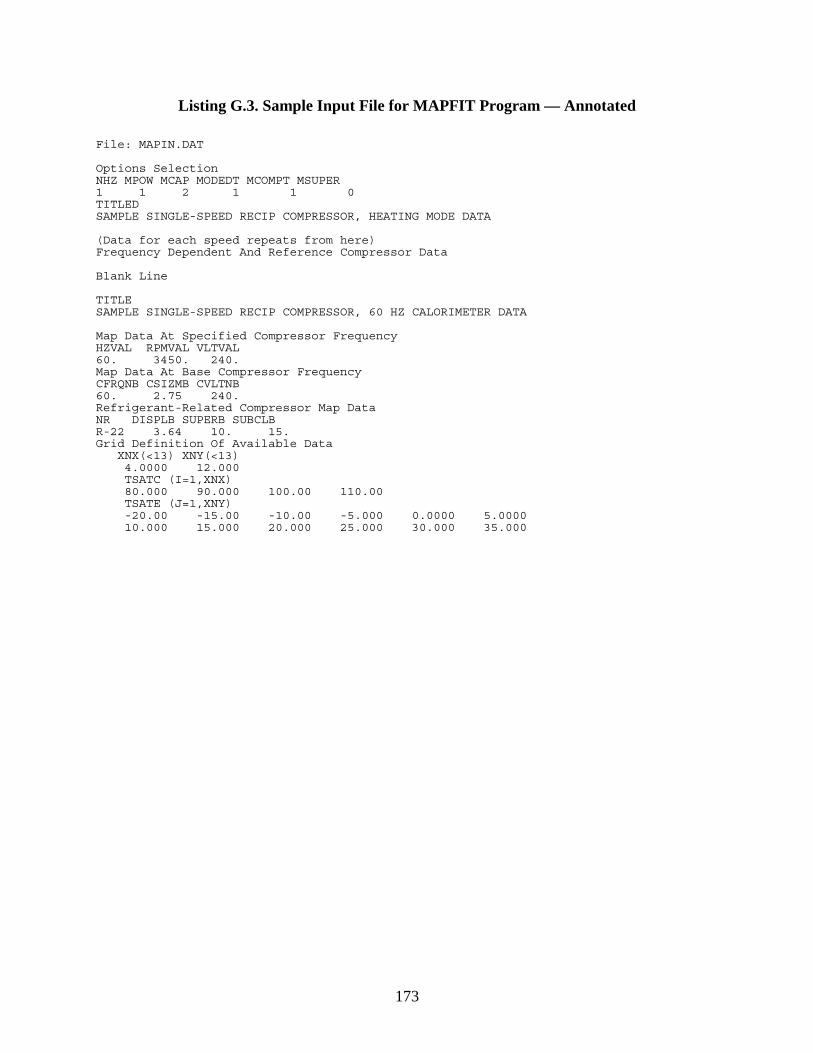
173
Listing G.3. Sample Input File for MAPFIT Program — Annotated
File: MAPIN.DAT
Options SelectionNHZ MPOW MCAP MODEDT MCOMPT MSUPER1 1 2 1 1 0TITLEDSAMPLE SINGLE-SPEED RECIP COMPRESSOR, HEATING MODE DATA
(Data for each speed repeats from here)Frequency Dependent And Reference Compressor Data
Blank Line
TITLESAMPLE SINGLE-SPEED RECIP COMPRESSOR, 60 HZ CALORIMETER DATA
Map Data At Specified Compressor Frequency HZVAL RPMVAL VLTVAL60. 3450. 240.Map Data At Base Compressor Frequency CFRQNB CSIZMB CVLTNB60. 2.75 240. Refrigerant-Related Compressor Map DataNR DISPLB SUPERB SUBCLBR-22 3.64 10. 15. Grid Definition Of Available Data XNX(<13) XNY(<13) 4.0000 12.000 TSATC (I=1,XNX) 80.000 90.000 100.00 110.00 TSATE (J=1,XNY) -20.00 -15.00 -10.00 -5.000 0.0000 5.0000 10.000 15.000 20.000 25.000 30.000 35.000

174
Listing G.3. Sample Input File for MAPFIT Program — Annotated (continued)
Data For Compressor Power Consumption
TITLE1 (for power data)SAMPLE MAP DATA FOR POWER CONSUMPTION (W) FOR HEATING MODE OPERATIONPower Data (W or kW as selected by MPOW on line 1)POWER(XNY,1) 1467.4 1605.0 1725.2 1860.6 1980.8 2092.3 2195.1 2293.5 2381.1 2464.4 2538.9 2606.9POWER(XNY,2) 1454.4 1598.5 1731.7 1871.5 2002.5 2124.9 2236.4 2345.7 2442.0 2536.1 2621.5 2698.2POWER(XNY,3) 1439.2 1587.6 1740.4 1888.9 2028.6 2164.0 2295.1 2417.4 2531.1 2644.8 2743.2 2841.7POWER(XNY,XNX) 1419.6 1583.3 1751.3 1910.6 2063.4 2216.2 2358.1 2500.1 2635.5 2768.7 2886.7 3000.4Weighting DataWGHT1(XNY,1) 1.0000 1.0000 1.0000 1.0000 1.0000 1.0000 1.0000 1.0000 1.0000 1.0000 1.0000 1.0000WGHT1(XNY,2) 1.0000 1.0000 1.0000 1.0000 1.0000 1.0000 1.0000 1.0000 1.0000 1.0000 1.0000 1.0000WGHT1(XNY,3) 1.0000 1.0000 1.0000 1.0000 1.0000 1.0000 1.0000 1.0000 1.0000 1.0000 1.0000 1.0000WGHT1(XNY,XNX) 1.0000 1.0000 1.0000 1.0000 1.0000 1.0000 1.0000 1.0000 1.0000 1.0000 1.0000 1.0000

175
Listing G.3. Sample Input File for MAPFIT Program — Annotated (continued)
Data For Refrigerant Mass Flow Rate Or Capacity
TITLE2 (for mass flow data)SAMPLE MAP DATA FOR MASS FLOW RATE (LBM/HR) FOR HEATING MODE OPERATION Mass Flow(lbm/h) or Capacity(kBtuh) Data (as selected by MCAP on line 1)XMR(XNY,1) 87.926 108.84 131.94 160.48 189.55 224.63 263.50 306.73 355.40 410.06 467.43 534.06 XMR(XNY,2) 80.308 100.13 123.77 152.32 181.94 217.01 253.71 293.67 339.08 387.75 438.05 495.43 XMR(XNY,3) 71.602 91.430 115.07 142.52 171.05 204.49 241.19 280.06 323.30 371.42 421.18 476.38 XMR(XNY,XNX) 62.349 83.268 106.36 133.82 161.80 194.70 230.31 266.46 308.61 353.47 399.41 452.44Weighting Data WGHT2(XNY,1) 1.0000 1.0000 1.0000 1.0000 1.0000 1.0000 1.0000 1.0000 1.0000 1.0000 1.0000 1.0000WGHT2(XNY,2) 1.0000 1.0000 1.0000 1.0000 1.0000 1.0000 1.0000 1.0000 1.0000 1.0000 1.0000 1.0000WGHT2(XNY,3) 1.0000 1.0000 1.0000 1.0000 1.0000 1.0000 1.0000 1.0000 1.0000 1.0000 1.0000 1.0000WGHT2(XNY,XNX) 1.0000 1.0000 1.0000 1.0000 1.0000 1.0000 1.0000 1.0000 1.0000 1.0000 1.0000 1.0000
Repeat data for additional speeds (N=1,NHZ)


177
Listing G.4. Sample Output Listing for MAPFIT Program
FILE: MAPOUT.DAT
SAMPLE SINGLE-SPEED RECIP COMPRESSOR, HEATING MODE DATA
SAMPLE MAP DATA FOR POWER CONSUMPTION (W) FOR HEATING MODE OPERATION INPUT DATA FOR MAP COMPRESSOR POWER CONSUMPTION:
MOTOR DRIVE FREQUENCY 60.0 HZ MOTOR NOMINAL SPEED 3450.0 RPM MOTOR VOLTAGE 240.0 VOLTS REFRIGERANT R-22 COMPRESSOR DISPLACEMENT 3.6400 CU IN MAP SUBCOOLING VALUE 15.00 F MAP SUPERHEAT VALUE 10.00 F
COMPRESSOR POWER CONSUMPTION INPUT DATA IS IN WATTS — IT HAS BEEN CONVERTED TOKILOWATTSEVAPORATING CONDENSING TEMPERATURE (F)TEMPERATURE (F) 80.00 90.00 100.00 110.00 _______________ _________ _________ _________ _________ -20.0 I DATA 1.4674 1.4544 1.4392 1.4196 I WEIGHT 1.0000 1.0000 1.0000 1.0000 -15.0 I DATA 1.6050 1.5985 1.5876 1.5833 I WEIGHT 1.0000 1.0000 1.0000 1.0000 -10.0 I DATA 1.7252 1.7317 1.7404 1.7513 I WEIGHT 1.0000 1.0000 1.0000 1.0000 -5.0 I DATA 1.8606 1.8715 1.8889 1.9106 I WEIGHT 1.0000 1.0000 1.0000 1.0000 .0 I DATA 1.9808 2.0025 2.0286 2.0634 I WEIGHT 1.0000 1.0000 1.0000 1.0000 5.0 I DATA 2.0923 2.1249 2.1640 2.2162 I WEIGHT 1.0000 1.0000 1.0000 1.0000 10.0 I DATA 2.1951 2.2364 2.2951 2.3581 I WEIGHT 1.0000 1.0000 1.0000 1.0000 15.0 I DATA 2.2935 2.3457 2.4174 2.5001 I WEIGHT 1.0000 1.0000 1.0000 1.0000 20.0 I DATA 2.3811 2.4420 2.5311 2.6355 I WEIGHT 1.0000 1.0000 1.0000 1.0000 25.0 I DATA 2.4644 2.5361 2.6448 2.7687 I WEIGHT 1.0000 1.0000 1.0000 1.0000 30.0 I DATA 2.5389 2.6215 2.7432 2.8867 I WEIGHT 1.0000 1.0000 1.0000 1.0000 35.0 I DATA 2.6069 2.6982 2.8417 3.0004 I WEIGHT 1.0000 1.0000 1.0000 1.0000

178
Listing G.4. Sample Output Listing for MAPFIT Program (continued)
SAMPLE MAP DATA FOR MASS FLOW RATE (LBM/HR) FOR HEATING MODE OPERATION INPUT (OR DERIVED) DATA FOR REFRIGERANT MASS FLOW RATE:
MOTOR DRIVE FREQUENCY 60.0 HZ MOTOR NOMINAL SPEED 3450.0 RPM MOTOR VOLTAGE 240.0 VOLTS REFRIGERANT R-22 COMPRESSOR DISPLACEMENT 3.6400 CU IN MAP SUBCOOLING VALUE 15.00 F MAP SUPERHEAT VALUE 10.00 F
EVAPORATING CONDENSING TEMPERATURE (F) TEMPERATURE (F) 80.00 90.00 100.00 110.00 _______________ _________ _________ _________ _________ -20.0 I DATA 87.9260 80.3080 71.6020 62.3490 I WEIGHT 1.0000 1.0000 1.0000 1.0000 -15.0 I DATA 108.8400 100.1300 91.4300 83.2680 I WEIGHT 1.0000 1.0000 1.0000 1.0000 -10.0 I DATA 131.9400 123.7700 115.0700 106.3600 I WEIGHT 1.0000 1.0000 1.0000 1.0000 -5.0 I DATA 160.4800 152.3200 142.5200 133.8200 I WEIGHT 1.0000 1.0000 1.0000 1.0000 .0 I DATA 189.5500 181.9400 171.0500 161.8000 I WEIGHT 1.0000 1.0000 1.0000 1.0000 5.0 I DATA 224.6300 217.0100 204.4900 194.7000 I WEIGHT 1.0000 1.0000 1.0000 1.0000 10.0 I DATA 263.5000 253.7100 241.1900 230.3100 I WEIGHT 1.0000 1.0000 1.0000 1.0000 15.0 I DATA 306.7300 293.6700 280.0600 266.4600 I WEIGHT 1.0000 1.0000 1.0000 1.0000 20.0 I DATA 355.4000 339.0800 323.3000 308.6100 I WEIGHT 1.0000 1.0000 1.0000 1.0000 25.0 I DATA 410.0600 387.7500 371.4200 353.4700 I WEIGHT 1.0000 1.0000 1.0000 1.0000 30.0 I DATA 467.4300 438.0500 421.1800 399.4100 I WEIGHT 1.0000 1.0000 1.0000 1.0000 35.0 I DATA 534.0600 495.4300 476.3800 452.4400 I WEIGHT 1.0000 1.0000 1.0000 1.0000

179
Listing G.4. Sample Output Listing for MAPFIT Program (continued)
SAMPLE SINGLE-SPEED RECIP COMPRESSOR, 60 HZ CALORIMETER DATA POWER CONSUMPTION (KW) COEFFICIENTS FOR BI-QUADRATIC FIT:
F(X,Y)= 6.6604E-05*X*X + -9.4360E-03*X + -1.2626E-04*Y*Y + 6.1468E-04*Y + 2.7157E-04*X*Y + 2.3063E+00
EVAPORATING CONDENSING TEMPERATURE (F) TEMPERATURE (F) 80.00 90.00 100.00 110.00 _______________ _________ _________ _________ _________ -20.0 I FIT 1.4804 1.4449 1.4228 1.4140 I MAP 1.4674 1.4544 1.4392 1.4196 I % .8856 -.6499 -1.1381 -.3934 -15.0 I FIT 1.6142 1.5923 1.5838 1.5885 I MAP 1.6050 1.5985 1.5876 1.5833 I % .5728 -.3864 -.2409 .3315 -10.0 I FIT 1.7417 1.7334 1.7384 1.7568 I MAP 1.7252 1.7317 1.7404 1.7513 I % .9551 .0974 -.1139 .3123 -5.0 I FIT 1.8628 1.8681 1.8867 1.9187 I MAP 1.8606 1.8715 1.8889 1.9106 I % .1209 -.1796 -.1140 .4228 .0 I FIT 1.9777 1.9966 2.0288 2.0743 I MAP 1.9808 2.0025 2.0286 2.0634 I % -.1561 -.2958 .0081 .5269 5.0 I FIT 2.0863 2.1187 2.1645 2.2236 I MAP 2.0923 2.1249 2.1640 2.2162 I % -.2889 -.2917 .0216 .3319 10.0 I FIT 2.1885 2.2345 2.2939 2.3665 I MAP 2.1951 2.2364 2.2951 2.3581 I % -.3012 -.0844 -.0542 .3572 15.0 I FIT 2.2844 2.3440 2.4169 2.5032 I MAP 2.2935 2.3457 2.4174 2.5001 I % -.3964 -.0720 -.0193 .1232 20.0 I FIT 2.3740 2.4472 2.5337 2.6335 I MAP 2.3811 2.4420 2.5311 2.6355 I % -.2976 .2128 .1027 -.0750 25.0 I FIT 2.4573 2.5441 2.6442 2.7576 I MAP 2.4644 2.5361 2.6448 2.7687 I % -.2877 .3142 -.0246 -.4026 30.0 I FIT 2.5343 2.6346 2.7483 2.8753 I MAP 2.5389 2.6215 2.7432 2.8867 I % -.1816 .5008 .1855 -.3960 35.0 I FIT 2.6050 2.7189 2.8461 2.9867 I MAP 2.6069 2.6982 2.8417 3.0004 I % -.0745 .7663 .1553 -.4575
THE MAXIMUM % VARIATION FROM THE MAP VALUE 1.1381 THE WEIGHTED AVERAGE OF THE ABSOLUTE VALUES OF THE % VARIATIONS .3058 THE WEIGHTED AVERAGE OF THE % VARIATIONS -.0014 THE STANDARD DEVIATION FROM THE AVERAGE % VARIATION .3980

180
Listing G.4. Sample Output Listing for MAPFIT Program (continued)
SAMPLE SINGLE-SPEED RECIP COMPRESSOR, 60 HZ CALORIMETER DATA MASS FLOW RATE (LB/H) COEFFICIENTS FOR BI-QUADRATIC FIT:
F(X,Y)= 4.3090E-03*X*X + -1.9373E+00*X + 7.1893E-02*Y*Y + 9.2904E+00*Y + -3.0419E-02*X*Y + 3.2045E+02
EVAPORATING CONDENSING TEMPERATURE (F) TEMPERATURE (F) 80.00 90.00 100.00 110.00 _______________ _________ _________ _________ _________ -20.0 I FIT 84.6637 78.6994 73.5970 69.3563 I MAP 87.9260 80.3080 71.6020 62.3490 I % -3.7103 -2.0030 2.7862 11.2388 -15.0 I FIT 106.3667 98.8815 92.2581 86.4965 I MAP 108.8400 100.1300 91.4300 83.2680 I % -2.2724 -1.2469 .9057 3.8772 -10.0 I FIT 131.6644 122.6583 114.5139 107.2313 I MAP 131.9400 123.7700 115.0700 106.3600 I % -.2089 -.8982 -.4833 .8192 -5.0 I FIT 160.5568 150.0297 140.3643 131.5608 I MAP 160.4800 152.3200 142.5200 133.8200 I % .0478 -1.5036 -1.5125 -1.6882 .0 I FIT 193.0438 180.9957 169.8095 159.4850 I MAP 189.5500 181.9400 171.0500 161.8000 I % 1.8432 -.5190 -.7252 -1.4308 5.0 I FIT 229.1255 215.5565 202.8492 191.0038 I MAP 224.6300 217.0100 204.4900 194.7000 I % 2.0013 -.6698 -.8024 -1.8984 10.0 I FIT 268.8018 253.7118 239.4837 226.1173 I MAP 263.5000 253.7100 241.1900 230.3100 I % 2.0121 .0007 -.7075 -1.8205 15.0 I FIT 312.0728 295.4619 279.7128 264.8254 I MAP 306.7300 293.6700 280.0600 266.4600 I % 1.7419 .6102 -.1240 -.6134 20.0 I FIT 358.9385 340.8066 323.5365 307.1283 I MAP 355.4000 339.0800 323.3000 308.6100 I % .9956 .5092 .0732 -.4801 25.0 I FIT 409.3988 389.7460 370.9550 353.0257 I MAP 410.0600 387.7500 371.4200 353.4700 I % -.1612 .5148 -.1252 -.1257 30.0 I FIT 463.4538 442.2800 421.9681 402.5179 I MAP 467.4300 438.0500 421.1800 399.4100 I % -.8507 .9657 .1871 .7781 35.0 I FIT 521.1035 498.4088 476.5758 455.6047 I MAP 534.0600 495.4300 476.3800 452.4400 I % -2.4260 .6012 .0411 .6995
THE MAXIMUM % VARIATION FROM THE MAP VALUE 11.2388 THE WEIGHTED AVERAGE OF THE ABSOLUTE VALUES OF THE % VARIATIONS 1.2970 THE WEIGHTED AVERAGE OF THE % VARIATIONS .0884 THE STANDARD DEVIATION FROM THE AVERAGE % VARIATION 2.1667

181
Listing G.4. Sample Output Listing for MAPFIT Program (continued)
SAMPLE SINGLE-SPEED RECIP COMPRESSOR, 60 HZ CALORIMETER DATA
COMPARISON TABLE OF VALUES DERIVED FROM POWER / MASS FLOW CURVE FITS VERSUS DATA-BASED(MAP) VALUES
ISENTROPIC EFFICIENCY EVAPORATING CONDENSING TEMPERATURE (F) TEMPERATURE (F) 80.00 90.00 100.00 110.00 _______________ _________ _________ _________ _________ -20.0 I CAL .3467 .3592 .3680 .3739 I MAP .3633 .3642 .3540 .3348 I I % -4.5555 -1.3619 3.9695 11.6782 -15.0 I CAL .3737 .3850 .3911 .3929 I MAP .3846 .3883 .3867 .3795 I I % -2.8289 -.8638 1.1494 3.5340 -10.0 I CAL .4001 .4115 .4166 .4164 I MAP .4047 .4156 .4182 .4143 I I % -1.1530 -.9947 -.3698 .5053 -5.0 I CAL .4244 .4370 .4423 .4415 I MAP .4247 .4428 .4486 .4509 I I % -.0730 -1.3264 -1.4002 -2.1021 .0 I CAL .4457 .4604 .4669 .4664 I MAP .4369 .4614 .4703 .4756 I I % 2.0024 -.2238 -.7333 -1.9475 5.0 I CAL .4633 .4808 .4893 .4900 I MAP .4529 .4826 .4934 .5011 I I % 2.2968 -.3792 -.8238 -2.2229 10.0 I CAL .4766 .4977 .5088 .5114 I MAP .4658 .4972 .5122 .5227 I I % 2.3203 .0852 -.6537 -2.1699 15.0 I CAL .4852 .5105 .5250 .5301 I MAP .4750 .5070 .5255 .5340 I I % 2.1468 .6827 -.1047 -.7357 20.0 I CAL .4886 .5189 .5373 .5455 I MAP .4824 .5174 .5375 .5478 I I % 1.2971 .2958 -.0295 -.4054 25.0 I CAL .4866 .5225 .5455 .5574 I MAP .4860 .5215 .5461 .5559 I I % .1269 .1999 -.1006 .2781 30.0 I CAL .4788 .5211 .5493 .5655 I MAP .4820 .5187 .5493 .5589 I I % -.6703 .4625 .0016 1.1788 35.0 I CAL .4648 .5143 .5485 .5695 I MAP .4760 .5152 .5491 .5630 I I % -2.3533 -.1638 -.1140 1.1623
THE MAXIMUM % VARIATION FROM THE MAP VALUE 11.6782 THE WEIGHTED AVERAGE OF THE ABSOLUTE VALUES OF THE % VARIATIONS 1.3799 THE WEIGHTED AVERAGE OF THE % VARIATIONS .0940 THE STANDARD DEVIATION FROM THE AVERAGE % VARIATION 2.3264

182
Listing G.4. Sample Output Listing for MAPFIT Program (continued)
SAMPLE SINGLE-SPEED RECIP COMPRESSOR, 60 HZ CALORIMETER DATA
COMPARISON TABLE OF VALUES DERIVED FROM POWER / MASS FLOW CURVE FITS VERSUS DATA-BASED(MAP) VALUES
VOLUMETRIC EFFICIENCY EVAPORATING CONDENSING TEMPERATURE (F) TEMPERATURE (F) 80.00 90.00 100.00 110.00 _______________ _________ _________ _________ _________ -20.0 I CAL .4153 .3861 .3610 .3402 I MAP .4313 .3940 .3513 .3059 I I % -3.7103 -2.0030 2.7862 11.2389 -15.0 I CAL .4685 .4355 .4063 .3810 I MAP .4794 .4410 .4027 .3667 I I % -2.2724 -1.2469 .9057 3.8772 -10.0 I CAL .5219 .4862 .4539 .4251 I MAP .5230 .4906 .4562 .4216 I I % -.2089 -.8982 -.4833 .8192 -5.0 I CAL .5742 .5366 .5020 .4705 I MAP .5740 .5448 .5097 .4786 I I % .0478 -1.5036 -1.5125 -1.6882 .0 I CAL .6244 .5854 .5492 .5158 I MAP .6131 .5884 .5532 .5233 I I % 1.8432 -.5190 -.7253 -1.4308 5.0 I CAL .6716 .6318 .5946 .5599 I MAP .6584 .6361 .5994 .5707 I I % 2.0013 -.6698 -.8024 -1.8984 10.0 I CAL .7156 .6754 .6375 .6020 I MAP .7015 .6754 .6421 .6131 I I % 2.0121 .0007 -.7075 -1.8205 15.0 I CAL .7560 .7158 .6776 .6416 I MAP .7431 .7115 .6785 .6455 I I % 1.7419 .6102 -.1240 -.6134 20.0 I CAL .7929 .7528 .7147 .6784 I MAP .7850 .7490 .7141 .6817 I I % .9956 .5092 .0732 -.4801 25.0 I CAL .8260 .7864 .7485 .7123 I MAP .8274 .7824 .7494 .7132 I I % -.1612 .5148 -.1252 -.1257 30.0 I CAL .8557 .8166 .7791 .7432 I MAP .8630 .8088 .7776 .7374 I I % -.8506 .9657 .1871 .7781 35.0 I CAL .8818 .8434 .8065 .7710 I MAP .9038 .8384 .8062 .7656 I I % -2.4260 .6012 .0411 .6995
THE MAXIMUM % VARIATION FROM THE MAP VALUE 11.2389 THE WEIGHTED AVERAGE OF THE ABSOLUTE VALUES OF THE % VARIATIONS 1.2970 THE WEIGHTED AVERAGE OF THE % VARIATIONS .0884 THE STANDARD DEVIATION FROM THE AVERAGE % VARIATION 2.1667

183
Listing G.5. Output Format Description for MAPFIT Program
C ** DATA FORMAT OF MAP-FIT COEFFICIENTS FOR TRANSFER TO HPDATA FILE **CC SET DEFAULT VALUES FOR PARAMETERS NOT PROVIDED IN MAPIN.DATCC For Definitions of the Following DEFAULTS,C Refer to Line 9.1 Of The HPDATA Input Description, Table B.1C ICMPDT = 2 ICDVCH = 2 CSIZMT = CSIZMB CFRQNM = CFRQNB CVLTNM = CVLTNB CVLHZM = 1.0 ADJ1 = 1.0 ADJ2 = 1.0 C Besides the selected value for MODEDT,C Line 9.1 also requires values for — ICMPDT, ICDVCH, CSIZMT, CFRQNM, C CVLTNM, and CVLHZM. These additional data, defined in Table B.1, C identify both the base and selected compressor maps as to drive type C and the nominal characteristics of the selected compressor drive. C WRITE(IODATA,1001) TITLED WRITE(IODATA,1211) MODEDT,ICMPDT,ICDVCH, & CSIZMT,CFRQNM,CVLTNM,CVLHZM WRITE(IODATA,1210) NHZ, DISPLB, SUPERN, & CSIZMB,CFRQNB,CVLTNBC–>> FOR EACH DRIVE FREQUENCY
WRITE(IODATA,1209) HZVAL, RPMVAL, VLTVAL, ADJ1, ADJ2
–>IF MODEDT = 1
C PUNCH CURVE-FIT COEFFICIENTS FOR POWER AND MASS FLOW RATEC IN THE FORM READ BY ORNL HEAT PUMP MODELC WRITE(IODATA,1208) (CPOWER(I,IHZ),I=1,6) WRITE(IODATA,1208) (CMASSF(I,IHZ),I=1,6)C –>IF MODEDT = 2CC PUNCH CURVE FIT COEFFICIENTS FOR ISENTROPIC AND VOLUMETRIC EFFICIENCIESC IN FORM READ BY ORNL HEAT PUMP MODELC WRITE(IODATA,1208) (CETAIS(I,IHZ),I=1,6) WRITE(IODATA,1208) (CETAVL(I,IHZ),I=1,4)CC Note: The data file punched to file MAPCOEF.DAT or the user-named C alternative file can be inserted as Lines 9.0 - 9.7 of the HPDATA file as C described in Table B.1 of Appendix B of the ORNL MODCON User’s Guide.
C Only Line 9.1 may need adjustment by the user of the default valuesC depending on what type of compressor drive and displacement the user


185
Listing G.6. Sample Output File for MAPFIT Program
FILE: MAPCOEF.DAT
*** SAMPLE OUTPUT DATA FILE FROM ORNL MAPFIT PROGRAM IN FORMAT NEEDED FOR USE IN ORNL HEAT PUMP DATA INPUT
SAMPLE SINGLE-SPEED RECIP COMPRESSOR, HEATING MODE DATA 1 2 2 2.7500 60.0000 240.0000 1.0000 1 3.6400 10.0000 2.7500 60.0000 240.0000 60.0000 3450.0000 240.0000 1.0000 1.0000 6.660E-05-9.436E-03-1.263E-04 6.147E-04 2.716E-04 2.306E+00 4.309E-03-1.937E+00 7.189E-02 9.290E+00-3.042E-02 3.205E+02


187
Listing G.7. Sample Output File for MAPFIT Program — Annotated
FILE: MAPCOEF.DAT
*** SAMPLE OUTPUT DATA FILE FROM ORNL MAPFIT PROGRAM IN FORMAT NEEDED FOR USE IN ORNL HEAT PUMP DATA INPUT
TITLEDSAMPLE SINGLE-SPEED RECIP COMPRESSOR, HEATING MODE DATA
MODEDT ICMPDT ICDVCH CSIZMT CFRQNM CVLTNM CVLHZM 1 2 2 2.7500 60.0000 240.0000 1.0000
NHZ DISPLB SUPERB CSIZMB CFRQNB CVLTNB 1 3.6400 10.0000 2.7500 60.0000 240.0000
HZVAL RPMVAL VLTVAL ADJ1 ADJ260.0000 3450.0000 240.0000 1.0000 1.0000
(CPOWER(I,IHZ),I=1,6) 6.660E-05-9.436E-03-1.263E-04 6.147E-04 2.716E-04 2.306E+00and(CMASSF(I,IHZ),I=1,6) 4.309E-03-1.937E+00 7.189E-02 9.290E+00-3.042E-02 3.205E+02
orif MODEDT=2,(CETAIS(I,IHZ),I=1,6) and(CETAVL(I,IHZ),I=1,4)


189
APPENDIX H
AMBIENT/SPEED/CONTROL DATA FILE ‘CONTRL’FOR SELECTED AND DUAL–MODE
AMBIENT–vs–SPEED PERFORMANCE MAPPING
Input Data Definitions and Format
The ‘CONTRL’ data file is an optional additional input file which can be used in specialcircumstances when more control in needed over the ambient temperatures and relative humiditiesat which heat pump performance is to be evaluated. It can also be used to generate ambient vscompressor speed data sets for both heating and cooling conditions in one run with full operationalvariable control. The data file was developed originally to provide a means of generatingperformance data suitable for the ORNL Annual Performance Factor / Loads Model. As such, it isprovided more as a special purpose option than as an integral part of the basic design tool package.
Table H.1 describes the input data requirements for the optional CONTRL data file. The operationalvariable specification used in CONTRL is identical to that for the CONCHZ data file (althoughpotential users should note that the required data format is different). This input data file is read bythe default unit number of 24 although this can be easily changed in the BLOCK DATA routine withreference to Appendix D.
One known inconsistency with the present version is that if temperatures are selected that are not onregular grid intervals, a set of performance data will be punched which contains the starting andending temperature values and the number of temperatures but no information about what actualtemperatures were used within the temperature range. As such, these data sets should not be usedto generate contour plots unless the header values are edited to reflect the actual temperatures usedfor each grid location. Alternatively, a separate version of the CONDAT routine could be written topass the correct, more detailed, heading information to the version of the CONDAT routine calledfrom the APFDRV routine (to generate the CONSPD dataset as shown in Figure CDG1).
Sample Input File (Regular and Annotated)
This section contains regular and annotated listings, Listings H.1 and H.2, respectively, of a sample‘CONTRL’ data file. The regular listing represents the data set as directly used by the model whilethe annotated version of the same data set is labeled with the variable names as described inTable H.1. The annotated listing is provided as a visual reference to users modifying existing datasets.
The selected example given by file RATING.CTL can be used to generate heating and coolingperformance data at the DOE rating conditions for variable speed heat pumps. Operationalcharacteristics which are approximately optimal for the sample heat pump given by the heat pumpspecification file OFFDES.HPS are included in the CONTRL data set. (These were obtained fromthe benchmark performance analysis of Rice [1991].) The resultant performance data at low,intermediate, and high speeds, as required for the various ambients, can be used to generate DOEHSPF and SEER ratings for selected DOE regions.


191
Table H.1. Description of Optional CONTRL Input Data to MODCON Program
(Required Only If MODEGN = 3,4, or 5 in CONCHZ Data File)
Variable Name Variable Description Sample Value
OPERATIONAL CONTROL DATA
>>> Loop Over Heating and Cooling Mode Data — –> M=1, 2
>>>>> Heating Mode Data (M=1)
a) Ambient Data
Operational Line #1 FORMAT(I3)
NTMPSS(M) number of ambient temperatures for which 2heating (M=1) or cooling (M=2) performance is required
Operational Lines“I=1,NTPMSS(M)” FORMAT(6F8.3)
TOUT(I,M) ambient temperature (�F) 17.0RHOUT(I,M) ambient relative humidity 0.70TIN(I,M) indoor thermostat setting (�F) 70.0RHIN(I,M) indoor design relative humidity 0.50TSE(I,M) estimate of compressor inlet saturation temperature (�F) 10.0TSC(I,M) estimate of compressor outlet saturation temperature (�F) 10.0
b) Compressor Frequency Data
Operational Line #“NTPMSS(M)+2" FORMAT(I3)
NFRQSS(M) number of compressor speeds at which steady-stateheating-mode 4(M=1) or cooling-mode (M=2) heat pump data are required;
– value is set to 1 internally if load/frequency iteration is used
Operational Line # “NTPMSS(M)+3" FORMAT(6F8.3)
CMFRLO(M) lowest compressor frequency (Hz) 60.0CMFRHI(M) highest compressor frequency (Hz) 240.0CMFRRF(M) reference compressor frequency (Hz) for frequency ratio calculation 120.0
– if load/frequency iteration is not used;initial guess for required compressor frequency (Hz)
– if load/frequency iteration is used (not yet operational)

192
c) Control Variable Data
Operational Line # “NTPMSS(M)+4" FORMAT(I3)
NVAL(M) number of control variables to be user-specified 1
Operational Lines “J=1,NVAL(M)” FORMAT(2I3,2X,6F8.3)
NFUN(J,M) integer value selecting controlled parameter “y” where y = f(x) 1= 1, for compressor inlet superheat (F�)= 2, for condenser exit subcooling (F�)= 3, for indoor blower frequency (Hz)= 4, for outdoor fan frequency (Hz)= 5, for building load (kBtuh/h) — not fully operational
NIND(J,M) integer value selecting controlling parameter “x” 1= 1, for ambient temperature (�F)= 2, for compressor frequency (Hz)
Coefficients of linear control algorithm of the form y = (y2 – y1)/(x2 – x1) • (x – x1) + y1
VINDEP(J,1,M) selected value of x1 17.0
VINDEP(J,2,M) selected value of x2 47.0
VDEPEN(J,1,M) prescribed value of y1 5.0
VDEPEN(J,2,M) prescribed value of y2 20.0
VDEPLO(J,M) minimum-allowable value of y1 0.0
VDEPHI(J,M) maximum-allowable value of y2 30.0
>>>>> Repeat For Cooling Mode Data (M=2)
a) Ambient Data :NTMPSS(M),Lines I=1, NTMPSS(M)
TOUT(I,M),RHOUT(I,M),TIN(I,M),RHIN(I,M),TSE(I,M),TSC(I, M)
b) Compressor Frequency Data :
NFRQSS(M)CMFRLO(M), CMFRHI(M), CMFRRF(M)

193
c) Control Variable Data :
NVAL(M)Lines J=1, NVAL(M)
NFUN(J,M),NIND(J,M),VINDEP(J,1,M),VINDEP(J,2,M), . . .. . .VDEPEN(J,1,M),VDEPEN(J,2,M),VDEPLO(J,M),VDEPHI(J,M)
>>> Loop Complete Over Operational Parameter Data
OUTPUT CONTROL DATA
Steady-State Performance Data Output
Output Line #1 FORMAT(I3)
IPUNCH Integer flag to select if steady-state performance data file is to be created 1
� 1, no data file is desired= 1, steady-state data file will be created in a format suitable for use
in the ORNL APF Model
Supplemental Contour Data Sets
>>> Loop Over Heating and Cooling Mode Data — –> M=1, 2
>>>>> Heating Mode Data (M=1)
a) Ambients :
Output Line #2 FORMAT(I3,F8.3)
NAMBCN(M) If � 0, number of supplemental ambients 1If = –1, indicates value of REFX(M) is to be readIf = –99, shortcut way to indicate that no supplemental ambient
or frequency data sets are desired
REFX(M) Reference ambient value for secondary ambient-vs-frequencycontour data set [only used if NAMBCN(M) = –1]
Output Line #3 FORMAT(20I3)(if NAMBCN(M) > 0)
IAMBCN(M) Ordinal numbers of selected ambients relative to NTMPSS(M) 2

194
b) Compressor Frequencies :
Output Line #4 FORMAT(I3,F8.3)
NFRQCN(M) If � 0, number of supplemental frequencies 1If = –1, indicates value of REFY(M) is to be read
REFY(M) Reference frequency value for secondary ambient-vs-frequencycontour data set [only used if NFRQCN(M) = –1]
Output Line #5 FORMAT(20I3)(if NFRQCN(M) > 0)
IFRQCN(M) Ordinal numbers of selected frequencies relative to NFRQSS(M) 2
>>>>> Repeat For Cooling Mode Data (M=2), If NAMBCN(1) > –99
a) Ambients : NAMBCN(M), REFX(M)IAMBCN(M)
b) Compressor Frequencies :
NFRQCN(M), REFY(M)IFRQCN(M)
>>> Loop Complete Over Output Data

195
Listing H.1. Sample Control Data File ‘CONTRL’ —Selected Heating And Cooling Ambients With Operational-Variable Control
File: RATING.CTL
0417.0 0.68 70.0 0.58 8.0 95.035.0 0.70 70.0 0.58 28.0 95.047.0 0.72 70.0 0.58 40.0 90.062.0 0.72 70.0 0.58 55.0 90.0 06 50.0 180.0 180.0 04 1 2 50.0 180.0 1.0 1.0 1.0 1.0 2 2 50.0 180.0 10.0 24.0 10.0 24.0 3 2 50.0 180.0 64.8 95.0 64.8 95.0 4 2 50.0 180.0 37.1 55.3 37.1 55.3 0467.0 0.40 80.0 0.52 55.0 90.082.0 0.40 80.0 0.52 55.0 90.087.0 0.40 80.0 0.52 48.0 115.095.0 0.40 80.0 0.52 48.0 115.0 06 50.0 180.0 180.0 04 1 2 50.0 180.0 10.0 10.0 10.0 10.0 2 2 50.0 180.0 5.0 15.0 5.0 15.0 3 2 50.0 180.0 45.6 108.0 45.6 108.0 4 2 50.0 180.0 53.0 82.5 53.0 82.5 01 -1 17.0 -1 180.0 -1 95.0 -1 180.0


197
Listing H.2. Annotated Sample Control Data File ‘CONTRL’ —Selected Heating and Cooling Ambients With Operational-Variable Control
File: RATING.CTL
OPERATIONAL CONTROL DATA:>>> Loop Over Heating and Cooling Mode Data >>>>> Heating Mode Data
Ambient Data — Heating Mode:Number Of AmbientsNTMPSS 04Ambient Conditions and Sat. Temp. Guesses >>>I=1,NTPMSSTOUT RHOUT TIN RHIN TSE TSC17.0 0.68 70.0 0.58 8.0 95.035.0 0.70 70.0 0.58 28.0 95.047.0 0.72 70.0 0.58 40.0 90.062.0 0.72 70.0 0.58 55.0 90.0
Compressor Frequency Data — Heating Mode:Number Of Compressor FrequenciesNFRQSS 06Minimum, Maximum, and Reference Frequencies CMFRLO CMFRHI CMFRRF 50.0 180.0 180.0
Operational Data — Heating Mode:NVALS 04 >>>J=1,NVALSNFUN NIND VINDEP1 VINDEP2 VDEPEN1 VDEPEN2 VDEPLO VDEPHI 1 2 50.0 180.0 1.0 1.0 1.0 1.0 2 2 50.0 180.0 10.0 24.0 10.0 24.0 3 2 50.0 180.0 64.8 95.0 64.8 95.0 4 2 50.0 180.0 37.1 55.3 37.1 55.3

198
Listing H.2. Annotated Sample Control Data File ‘CONTRL’ —Selected Heating And Cooling Ambients With Operational-Variable Control
(continued)
>>>>> Cooling Mode Data
Ambient Data — Cooling Mode:Number Of AmbientsNTMPSS 04Ambient Conditions and Sat. Temp. Guesses >>>I=1,NTPMSSTOUT RHOUT TIN RHIN TSE TSC67.0 0.40 80.0 0.52 55.0 90.082.0 0.40 80.0 0.52 55.0 90.087.0 0.40 80.0 0.52 48.0 115.095.0 0.40 80.0 0.52 48.0 115.0
Compressor Frequency Data — Cooling Mode:Number Of Compressor Frequencies — Cooling ModeNFRQSS 06Minimum, Maximum, and Reference Frequencies CMFRLO CMFRHI CMFRRF 50.0 180.0 180.0
Operational Data — Cooling Mode:NVALS 04 >>>J=1,NVALSNFUN NIND VINDEP1 VINDEP2 VDEPEN1 VDEPEN2 VDEPLO VDEPHI 1 2 50.0 180.0 10.0 10.0 10.0 10.0 2 2 50.0 180.0 5.0 15.0 5.0 15.0 3 2 50.0 180.0 45.6 108.0 45.6 108.0 4 2 50.0 180.0 53.0 82.5 53.0 82.5
>>> End Of Operational Data Loop Over Heating and Cooling Modes

199
Listing H.2. Annotated Sample Control Data File ‘CONTRL’ —Selected Heating And Cooling Ambients With Operational-Variable Control
(continued)
OUTPUT CONTROL DATA:
Steady-State Performance Data OutputIPUNCH 01
SUPPLEMENTAL CONTOUR DATA SETS:
>>> Loop Over Heating and Cooling Mode Data
>>>>> Heating Mode DataReference Heating Ambient NAMBCN REFX -1 17.0Reference Heating Compressor FrequencyNFRQCN REFY -1 180.0
>>>>> Cooling Mode DataReference Cooling Ambient NAMBCN REFX-1 95.0Reference Cooling Compressor FrequencyNFRQCN REFY -1 180.0
>>> End Of Supplemental Contour Data Loop Over Heating and Cooling Modes