Embed Size (px)
Citation preview

Intro Lit Contr Shocks Tree EM Likelihood Results Goodness of Fit More IRR Distr Option Costs Contr
The Option Value of Educational Choices
And the Rate of Return to Educational Choices
James Heckman Sergio UrzuaUniversity of Chicago Northwestern University
University College Dublin
Institute for Computational Economics LectureUniversity of Chicago
August 1, 2008

Intro Lit Contr Shocks Tree EM Likelihood Results Goodness of Fit More IRR Distr Option Costs Contr
Introduction
Conventional models of rates of return to schooling followBecker (1964).
Assume perfect certainty.
Compare two earnings streams associated with schooling s ands ′, s < s ′:
Y (s, t) = earnings at schooling s at age t
Y (s ′, t) = earnings at schooling s ′ at age t
Usually years of schooling are assumed to be ordered.
Intro Lit Contr Shocks Tree EM Likelihood Results Goodness of Fit More IRR Distr Option Costs Contr
Introduction
Rate of return is computed from pairwise comparisons ofearnings streams.
Define costs of going from s → s ′ at time t as C (s ′, s, t),
0 =T∑
t=0
Y (s ′, t)− Y (s, t)− C (s ′, s, t)
(1 + ρ(s ′, s))t
Assumes pairwise earnings profiles cross, but only once.
ρ(s ′, s) is the pairwise rate of return.

Intro Lit Contr Shocks Tree EM Likelihood Results Goodness of Fit More IRR Distr Option Costs Contr
The “Mincer” model of earnings approximates ρ(s, s ′) underspecial conditions which are tested and rejected in U.S. data(Heckman, Lochner and Todd, 2006, 2008).
Main reasons for rejection:
(i) additive separability in log Y (s, t) between work experienceand schooling is violated,
(ii) the costs of schooling are more than earnings foregone andearnings in school do not cover tuition costs,
(iii) Cunha, Heckman and Navarro (2005) and Cunha andHeckman (2007,2008) document that huge “psychic costs” arerequired to rationalize schooling choices in an expected incomemaximizing model.

Intro Lit Contr Shocks Tree EM Likelihood Results Goodness of Fit More IRR Distr Option Costs Contr
As noted by Weisbrod (1962), pairwise comparisons betweenearnings streams associated with s and s ′ miss an importantcomponent of the return to the transition s to s ′.
Getting to s ′ means you have the option to go on to s ′′ > s ′.
The option value as defined by Weisbrod is the return thatarises from not having to stop at s ′ (to go onto higher levels ofeducation).
There is some confusion because Weisbrod’s “option value” isnot the value of an (American option).
Option values as defined by Weisbrod can arise even in anenvironment of prefect certainty.
True rates of return are underestimated by internal rates ofreturn.

Intro Lit Contr Shocks Tree EM Likelihood Results Goodness of Fit More IRR Distr Option Costs Contr
Heckman, Lochner and Todd (2006) show that the internalrate of return, ex ante is not in general the proper rate ofreturn criterion in a multiperiod (T ≥ 3) model withuncertainty and more than two schooling choices even ifearnings profiles cross only once in terms of age.
Discounted alternative earnings streams associated with valuefunction branches can cross multiply even if, for pairwiseschooling levels, they cross only once.
Intro Lit Contr Shocks Tree EM Likelihood Results Goodness of Fit More IRR Distr Option Costs Contr
Need a more general rate of return concept based on valuefunctions.
The rate of return cannot be defined independently of theinterest rate as in the simple Becker model.
IRR ≷ r does not answer the question whether there isunder-investment or over-investment in schooling.

Intro Lit Contr Shocks Tree EM Likelihood Results Goodness of Fit More IRR Distr Option Costs Contr
Summary of Current State of the Empirical Literature onReturns to Education
Preoccupation of most of the empirical literature with internalrates of return — IRR — in an environment of perfect certainty.
IRR a la Becker misses learning and option values arising fromlearning and nonlinearity in payoffs of education in years ofschooling
Mincer model seeks to approximate IRR and in general fails toidentify even IRR.
Need a model to capture these features plus psychic costs ofschooling.

Intro Lit Contr Shocks Tree EM Likelihood Results Goodness of Fit More IRR Distr Option Costs Contr
Need a model that recognizes that many educational choicesare not simply summarized by “years of schooling” as in theMincer model.
Thus {s} is not necessarily ordered: job training, etc.
In addition, people can drop in and drop out of school.
There are multiple decisions:
(a) Whether to move to a feasible schooling state(b) When to move
Both create options and we can define option values for each.

Intro Lit Contr Shocks Tree EM Likelihood Results Goodness of Fit More IRR Distr Option Costs Contr
Theoretical Contributions of this Paper
A dynamic sequential model of educational choices amongdiscrete states with option values arising from learning andnonlinearity of reward functions at different stages of the lifecycle.
We build a model of schooling connecting high school droppingout, GED attainment, delay, college choices and returns.
Define the correct concept of the rate of return to schooling ina dynamic model with uncertainty, nonlinearity and delay.
Builds on previous work on dynamic selection into schooling(Altonji, 1993; Keane and Wolpin, 1997, 2001; Eckstein andWolpin, 1999; Arcidiacono, 2004; Cameron and Heckman,1998, 2001).
Like Arcidiacono (2004), we model learning about persistentshocks (see also Miller, 1984; Pakes, 1986; and others).

Intro Lit Contr Shocks Tree EM Likelihood Results Goodness of Fit More IRR Distr Option Costs Contr
Our Model:
Agents are risk neutral.
Model is identified semiparametrically:
(i) non-parametric identification of distributions of unobservablesthat are serially persistent;
(ii) earnings equations parametric (but flexible functional forms).

Intro Lit Contr Shocks Tree EM Likelihood Results Goodness of Fit More IRR Distr Option Costs Contr
Empirical Contributions of This Paper
Estimate true rates of return and compare with IRR.
Decompose option values by stages (educational choices andtimes choices are made; account for delay).
Estimate at each stage the respective contributions ofnon-linearity and learning to option values and rates of return.
Estimate contributions of both cognitive and noncognitive skillsto returns and costs.
We analyze jointly high school dropout and GED returns, aswell as returns to two year and four year colleges(Eckstein-Wolpin, 1999).
Intro Lit Contr Shocks Tree EM Likelihood Results Goodness of Fit More IRR Distr Option Costs Contr
Relationship to Previous Work
Like Weisbrod (1962) and Altonji (1993), we recognize theoption value that comes from educational choices.
Like Levhari and Weiss (1974) and Keane and Wolpin (1997),we recognize uncertainty in post-educational earnings.
Like Altonji (1993), Arcidiacono (2004) and Santos (2008), werocognize the learning value of schooling.
Unlike Keane and Wolpin (1997, 2001), we consider seriallypersistent shocks which agents learn about (as in Miller 1984and Pakes 1986)
This produces much greater estimated option values than anindependent shock model.
We define and estimate the appropriate rate of return for adynamic model with serially persistent shocks, nonlinearity andlearning.

Intro Lit Contr Shocks Tree EM Likelihood Results Goodness of Fit More IRR Distr Option Costs Contr
Rate of Return to Schooling with Uncertainty, Learning AboutState-specific Shocks
Simple Model
Consider a simple economic model as prologue.
The model we estimate is much richer. This simple modelmotivates our analysis.
Periods and schooling levels are assumed to be the same.

Intro Lit Contr Shocks Tree EM Likelihood Results Goodness of Fit More IRR Distr Option Costs Contr
Each schooling level s characterized by a shock, εs .
More precisely, suppose that there is uncertainty about netearnings conditional on s, so that actual discounted lifetimeearnings for someone with s years of school are
Ys =
[T∑
x=0
(1 + r)−xY (s, x)
]εs .

Intro Lit Contr Shocks Tree EM Likelihood Results Goodness of Fit More IRR Distr Option Costs Contr
Rate of Return to Schooling with Uncertainty, Learning AboutState-specific Shocks
s is ordered; s ′ > s means more schooling in s.
A one time, schooling (state) specific shock.
Assume that E (εs | Is−1) = 1 and define expected earningsassociated with schooling s conditional on current schoolings − 1,
Ys = E (Ys | Is−1).

Intro Lit Contr Shocks Tree EM Likelihood Results Goodness of Fit More IRR Distr Option Costs Contr
Rate of Return to Schooling with Uncertainty, Learning AboutState-specific Shocks
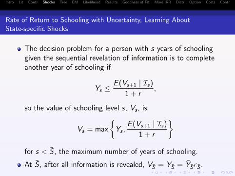
The decision problem for a person with s years of schoolinggiven the sequential revelation of information is to completeanother year of schooling if
Ys ≤E (Vs+1 | Is)
1 + r,
so the value of schooling level s, Vs , is
Vs = max
{Ys ,
E (Vs+1 | Is)
1 + r
}for s < S , the maximum number of years of schooling.
At S , after all information is revealed, VS = YS = YSεS .
Intro Lit Contr Shocks Tree EM Likelihood Results Goodness of Fit More IRR Distr Option Costs Contr
Rate of Return to Schooling with Uncertainty, Learning AboutState-specific Shocks
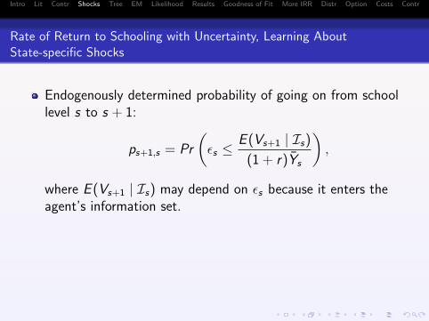
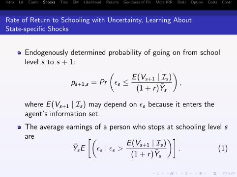
Endogenously determined probability of going on from schoollevel s to s + 1:
ps+1,s = Pr
(εs ≤
E (Vs+1 | Is)
(1 + r)Ys
),
where E (Vs+1 | Is) may depend on εs because it enters theagent’s information set.
The average earnings of a person who stops at schooling level sare
YsE
[(εs | εs >
E (Vs+1 | Is)
(1 + r)Ys
)]. (1)
Intro Lit Contr Shocks Tree EM Likelihood Results Goodness of Fit More IRR Distr Option Costs Contr
Rate of Return to Schooling with Uncertainty, Learning AboutState-specific Shocks
Endogenously determined probability of going on from schoollevel s to s + 1:
ps+1,s = Pr
(εs ≤
E (Vs+1 | Is)
(1 + r)Ys
),
where E (Vs+1 | Is) may depend on εs because it enters theagent’s information set.
The average earnings of a person who stops at schooling level sare
YsE
[(εs | εs >
E (Vs+1 | Is)
(1 + r)Ys
)]. (1)

Intro Lit Contr Shocks Tree EM Likelihood Results Goodness of Fit More IRR Distr Option Costs Contr
Rate of Return to Schooling with Uncertainty, Learning AboutState-specific Shocks
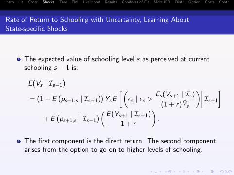
The expected value of schooling level s as perceived at currentschooling s − 1 is:
E (Vs | Is−1)
= (1− E (ps+1,s | Is−1)) YsE
[(εs | εs >
Es(Vs+1 | Is)
(1 + r)Ys
)∣∣∣∣ Is−1
]+ E (ps+1,s | Is−1)
(E (Vs+1 | Is−1)
1 + r
).
The first component is the direct return. The second componentarises from the option to go on to higher levels of schooling.
Intro Lit Contr Shocks Tree EM Likelihood Results Goodness of Fit More IRR Distr Option Costs Contr
Rate of Return to Schooling with Uncertainty, Learning AboutState-specific Shocks
The expected value of schooling level s as perceived at currentschooling s − 1 is:
E (Vs | Is−1)
= (1− E (ps+1,s | Is−1)) YsE
[(εs | εs >
Es(Vs+1 | Is)
(1 + r)Ys
)∣∣∣∣ Is−1
]+ E (ps+1,s | Is−1)
(E (Vs+1 | Is−1)
1 + r
).
The first component is the direct return. The second componentarises from the option to go on to higher levels of schooling.

Intro Lit Contr Shocks Tree EM Likelihood Results Goodness of Fit More IRR Distr Option Costs Contr
Rate of Return to Schooling with Uncertainty, Learning AboutState-specific Shocks
If schooling choices are irreversible, the option value ofschooling s, as perceived after completing s − 1 levels ofschooling is
Os,s−1 = E ([Vs − Ys ] | Is−1) .
Value of schooling is E (Vs | Is−1).

Intro Lit Contr Shocks Tree EM Likelihood Results Goodness of Fit More IRR Distr Option Costs Contr
Rate of Return to Schooling with Uncertainty, Learning AboutState-specific Shocks
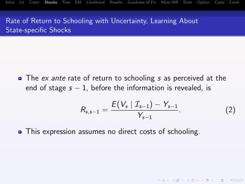
The ex ante rate of return to schooling s as perceived at theend of stage s − 1, before the information is revealed, is
Rs,s−1 =E (Vs | Is−1)− Ys−1
Ys−1. (2)
This expression assumes no direct costs of schooling.
Intro Lit Contr Shocks Tree EM Likelihood Results Goodness of Fit More IRR Distr Option Costs Contr
Rate of Return to Schooling with Uncertainty, Learning AboutState-specific Shocks
The ex ante rate of return to schooling s as perceived at theend of stage s − 1, before the information is revealed, is
Rs,s−1 =E (Vs | Is−1)− Ys−1
Ys−1. (2)
This expression assumes no direct costs of schooling.

Intro Lit Contr Shocks Tree EM Likelihood Results Goodness of Fit More IRR Distr Option Costs Contr
Rate of Return to Schooling with Uncertainty, Learning AboutState-specific Shocks
If there are up-front direct costs of schooling, Cs−1, to advancebeyond level s − 1, the ex ante return is
Rs,s−1 =E (Vs | Is−1)− (Ys−1 + Cs−1)
Ys−1 + Cs−1.
This expression assumes that tuition or direct costs are incurredup front and that returns are revealed one period later.
Intro Lit Contr Shocks Tree EM Likelihood Results Goodness of Fit More IRR Distr Option Costs Contr
Rate of Return to Schooling with Uncertainty, Learning AboutState-specific Shocks
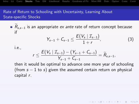
Rs,s−1 is an appropriate ex ante rate of return concept becauseif
Ys−1 + Cs−1 ≤E (Vs | Is−1)
1 + r, (3)
i.e.,
r ≤ E (Vs | Is−1)− (Ys−1 + Cs−1)
Ys−1 + Cs−1= Rs,s−1,
then it would be optimal to advance one more year of schooling(from s − 1 to s) given the assumed certain return on physicalcapital r .
The ex post return as of period s is
Vs − (Ys−1 + Cs−1)
Ys−1 + Cs−1.

Intro Lit Contr Shocks Tree EM Likelihood Results Goodness of Fit More IRR Distr Option Costs Contr
Rate of Return to Schooling with Uncertainty, Learning AboutState-specific Shocks
The distinction between ex ante and ex post returns toschooling is an important one that is not made in theconventional literature on “returns to schooling” surveyed inWillis (1986) or Katz and Autor (1999).
Levhari and Weiss (1974) and Altonji (1993) make thisdistinction.

Intro Lit Contr Shocks Tree EM Likelihood Results Goodness of Fit More IRR Distr Option Costs Contr
Example
Illustrate the role of uncertainty and non-linearity of logearnings in terms of schooling.
Simulate a five schooling-level version of the model withuncertainty.
Assume an interest rate of r = 0.1.
Further assume that εs is independent and identicallydistributed log-normal: log(εs) ∼ N(0, σ) for all s.
Assume that σ = 0.1 in the results presented in the tables.

Intro Lit Contr Shocks Tree EM Likelihood Results Goodness of Fit More IRR Distr Option Costs Contr
Simulated Returns under Uncertainty with Option Values
(Log Wages Linear in Schooling: Ys+1 = (1 + r)Ys)
Educ. Transition Proportional Proportional Option/ Avg. Return
Level Probability Increase Increase in Total Value E(Rs,s−1 | Is ) Treatment Treatment
(s) (ps,s−1) in Y ObservedOs,s−1
E(Vs | Is−1)on on
Earnings Treated Untreated
2 0.796 0.100 0.086 0.075 0.201 0.242 0.0413 0.746 0.100 0.082 0.060 0.182 0.231 0.0374 0.669 0.100 0.072 0.038 0.155 0.216 0.0325 0.520 0.100 0.016 0.000 0.111 0.196 0.019
OLS (Mincer) estimate of the rate of return is 0.063.
(Sheepskin Effects: Ys+1 = (1 + ρs+1)Ys with ρ2 = 0.1, ρ3 = 0.3, ρ4 = 0.1, ρ5 = 0.2)
2 0.997 0.100 0.101 0.239 0.459 0.460 0.0683 0.997 0.300 0.116 0.100 0.459 0.460 0.0684 0.846 0.100 0.092 0.093 0.224 0.257 0.0455 0.822 0.200 0.041 0.000 0.212 0.249 0.043
OLS (Mincer) estimate of the rate of return is 0.060.
Intro Lit Contr Shocks Tree EM Likelihood Results Goodness of Fit More IRR Distr Option Costs Contr
Notes
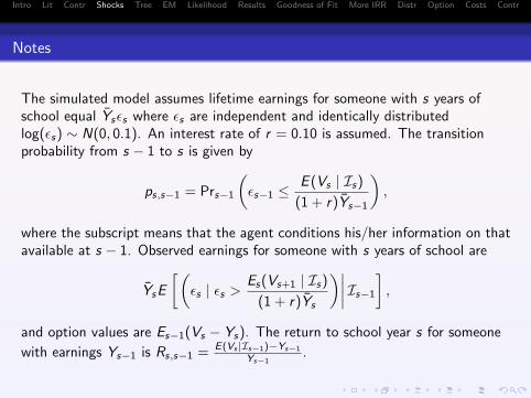
The simulated model assumes lifetime earnings for someone with s years ofschool equal Ysεs where εs are independent and identically distributedlog(εs) ∼ N(0, 0.1). An interest rate of r = 0.10 is assumed. The transitionprobability from s − 1 to s is given by
ps,s−1 = Prs−1
(εs−1 ≤
E (Vs | Is)
(1 + r)Ys−1
),
where the subscript means that the agent conditions his/her information on thatavailable at s − 1. Observed earnings for someone with s years of school are
YsE
[(εs | εs >
Es(Vs+1 | Is)
(1 + r)Ys
)∣∣∣∣ Is−1
],
and option values are Es−1(Vs − Ys). The return to school year s for someone
with earnings Ys−1 is Rs,s−1 = E(Vs |Is−1)−Ys−1
Ys−1.

Intro Lit Contr Shocks Tree EM Likelihood Results Goodness of Fit More IRR Distr Option Costs Contr
Notes (cont.)
Average returns reflect the expected return over the full distribution of Ys−1, orEs−1[Rs,s−1]. “Treatment on Treated” reflects returns for those who continueto grade s, or
E
[Rs,s−1 | εs−1 ≤
Es−1(Vs | Is)
(1 + r)Ys−1
∣∣∣∣ Is−1
].
“Treatment on Untreated” reflects returns for those who do not continue tograde s, or
E
[Rs,s−1 | εs−1 >
Es−1(Vs | Is)
(1 + r)Ys−1
∣∣∣∣ Is−1
].
The marginal treatment effect equals r = 0.10. OLS (Mincer) estimate is thecoefficient on schooling in a log earnings regression (the Mincer return).

Intro Lit Contr Shocks Tree EM Likelihood Results Goodness of Fit More IRR Distr Option Costs Contr
A More General Model with Delay, Dropout and Return
Our Data: The Decision Tree Agents Face
Educational choice s is made at time t, t ∈ {1, . . . ,T}.
The set {s(1), . . . , s(T )} is not necessarily ordered.

Given High School Enrollment at Age 18 — Top of TreeFigure 1. Evolution of Education AchievedNLSY79 - White Males
14s1 17s1 18s2 19s1 – 24s2 26s2
EHS (1954)
HSD (210)
HSD (188)
HSD (172)
HSD (156) HSD (156) HSD (156)
GED (16)
GED (11) GED (11)
ECO (5) COL (5)
GED (16)
GED (11) GED (11) GED (11)
ECO (5) COL (5) COL (5)
GED (22)
GED (9) GED (9) GED (9) GED (9)
ECO (13) COL (13) COL (13) COL (13)
EHS (1744)
EHS (433)
HSD (159)
HSD (111) HSD (111) HSD (111)
GED (48)
GED (33) GED (33)
ECO (15) COG (15)
HSG (274)
HSG (163) HSG (163) HSG (163)
ECO (111)
SCO (98) SCO (98)
COG (13) COG (13)
HSG (1311)
HSG (579)
HSG (437) HSG (437) HSG (437)
ECO (142)
SCO (103) SCO (103)
COG (39) COG (39)
ECO (732)
SCO (171) SCO (171) SCO (171)
COG (561) COG (561) COG (561)
14s1 17s1 18s2 20s2 22s2 24s2 26s2
EHS = Enrolled in High School HSG = High School GraduateHSD = High School Dropout ECO = Enrolled in CollegeSCO = Some College Completed GED = GED Completed
Note: All figures are in 2000 US Dollars.
1

Given High School Enrollment at Age 19 — Bottom of Tree
Figure 1. Evolution of Education AchievedNLSY79 - White Males
14s1 17s1 18s2 19s1 – 24s2 26s2
EHS (1954)
HSD (210)
HSD (188)
HSD (172)
HSD (156) HSD (156) HSD (156)
GED (16)
GED (11) GED (11)
ECO (5) COL (5)
GED (16)
GED (11) GED (11) GED (11)
ECO (5) COL (5) COL (5)
GED (22)
GED (9) GED (9) GED (9) GED (9)
ECO (13) COL (13) COL (13) COL (13)
EHS (1744)
EHS (433)
HSD (159)
GED (48)
GED (33) GED (33)
ECO (15) COG (15)
HSG (274)
HSG (163) HSG (163) HSG (163)
ECO (111)
SCO (98) SCO (98)
COG (13) COG (13)
HSG (1311)
HSG (579)
HSG (437) HSG (437) HSG (437)
ECO (142)
SCO (103) SCO (103)
COG (39) COG (39)
ECO (732)
SCO (171) SCO (171) SCO (171)
COG (561) COG (561) COG (561)
14s1 17s1 18s2 20s2 22s2 24s2 26s2
EHS = Enrolled in High School HSG = High School GraduateHSD = High School Dropout ECO = Enrolled in CollegeSCO = Some College Completed GED = GED Completed
Note: All figures are in 2000 US Dollars.
1

Evolution of Schooling AttainmentGiven High School Enrollment at Age 19 — Top of Tree
NLSY79 — White MalesEvolution of Schooling AttainmentGiven High School Enrollment at Age 19–Top of Tree
NLSY79 - White Males, June 9, 2008
HSGr579
EnCo142
E4Co67
4Co 39 4Co 39
S4Co28
S4Co28
E2Co75
2Co 32 2Co 32 2Co 32
S2Co43
S2Co43
S2Co43
HSGr437
HSGr437
HSGr437
HSGr437
Age 19 Age 20 Age 20 Age 21 Age 22 Age 23 Age 24 Age 26
HSGr = High School Graduate EnCo = Enrolled in CollegeEnNCo = Enrolled in N -Year College SNCO = Some N -Year CollegeNCo = N -Year College Completed
1

Intro Lit Contr Shocks Tree EM Likelihood Results Goodness of Fit More IRR Distr Option Costs Contr
State Space
(1) Information may arrive in each state and at each age;
(2) Information can be state specific (e.g. you learn somethingabout yourself by going to college but you do not learn if you donot go to college).
(3) I(s, t) is the information set.
(4) Specify a (state)×(age) specification (s, t).

Intro Lit Contr Shocks Tree EM Likelihood Results Goodness of Fit More IRR Distr Option Costs Contr
Economic Model
At each age t and state s there is a current period net reward.
R(s, t), s ∈ S, t ∈ {1, . . . ,T}
Assume exponential discounting for this paper.
This is relaxed in work underway.
I(s, t) is the information set in state s at time t.
s(t) ∈ S is the choice agents make at age t.
Full state at t is (s(t), t, I(s, t)).
Assume a non-stochastic discount rate r .
κ(s, t) is choice set open to a person when they are at schooling sat time t.

Intro Lit Contr Shocks Tree EM Likelihood Results Goodness of Fit More IRR Distr Option Costs Contr
At time t in state s, agent has a sequence of possible future choices.
κ(s, t) depends on current information I(s, t).
The agent’s value function at time t is
V (s(t), t | I(s, t)) = max[s(τ) ∈ κ(s, τ)]τ≥t
E
T∑τ≥t
R(s(τ), τ)
(1 + r)τ−t
∣∣∣∣ I(s, t)
.
Intro Lit Contr Shocks Tree EM Likelihood Results Goodness of Fit More IRR Distr Option Costs Contr
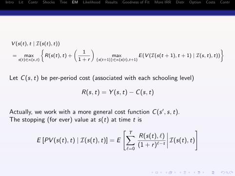
V (s(t), t | I(s(t), t))
= maxs(t)∈κ(s,t)
{R(s(t), t) +
(1
1 + r
)max
{s(t+1)}∈κ(s(t),t+1)E(V (I(s(t + 1), t + 1) | I(s, t), t))
}
Let C (s, t) be per-period cost (associated with each schooling level)
R(s, t) = Y (s, t)− C (s, t)
Actually, we work with a more general cost function C (s ′, s, t).The stopping (for ever) value at s(t) at time t is
E [PV (s(t), t) | I(s(t), t)] = E
[T∑
`=0
R(s(t), `)
(1 + r)`−t
∣∣∣∣ I(s(t), t)
]

Intro Lit Contr Shocks Tree EM Likelihood Results Goodness of Fit More IRR Distr Option Costs Contr
There are a variety of possible option values.
Consider a simple schooling model that illustrates our main points.

Intro Lit Contr Shocks Tree EM Likelihood Results Goodness of Fit More IRR Distr Option Costs Contr
Figure: American Option
Buy
Strike
... ...
Strike Strike Strike Strike Strike
0 1 2 3 4 5ContinueContinueContinueContinueContinueContinue
Period
Option value: What you pay to have the “right to strike” indifferent periods. (Initial price given initial information.)
If you strike, you get the value of the portfolio in that period.
You get no current flow if you continue.
Option value is price of this stream at date “0”
Continuation values can be computed at each stage.

Intro Lit Contr Shocks Tree EM Likelihood Results Goodness of Fit More IRR Distr Option Costs Contr
Figure: Standard Schooling Model with Irreversible Choices (Once youstop, you cannot return)
... ...
0 1 2 3 4 5
Enroll
DDDD DD
C CCCC CC
D = Dropout C = Continue
Each stage is one period.
This is the “standard” framework (consistent with Mincer).
By analogy with the American options literature, one definition of the option value isthe value of the program associated with enrolling and being able to drop out.
Unlike that case, you can get a flow if you continue.
The option value can be computed up front or at each stage. (continuation value)
The pairwise internal rates of return compare one of the many branches with the other.

Intro Lit Contr Shocks Tree EM Likelihood Results Goodness of Fit More IRR Distr Option Costs Contr
Figure:
... ...
0 1 2 3 4 5
Enroll
DDDD DD
C CCCC CC
... ...
0 1 2 3 4 5
Enroll
DDDD DD
C CCCC CC
= A = B
Compare A with B (two of many possible choices)

Intro Lit Contr Shocks Tree EM Likelihood Results Goodness of Fit More IRR Distr Option Costs Contr
Figure: More General
... ...
0
1
Enroll
D
DD
C CC
CR
R
D = Dropout C = Continue
R = Re-enroll
DD ... ...
... ...
... ...
2 3
D
C
Two dimensions: Level attained and when it is attainedCan define “option value” as return to the more general programOr value of“options” open up by attaining a level of schooling

Intro Lit Contr Shocks Tree EM Likelihood Results Goodness of Fit More IRR Distr Option Costs Contr
Option Value of College Calculation Schematic
Traditional High School Path
EnHS
EnHS
HSGr
Coll Coll
HSGrColl
HSGr
Drop
GEDColl
GED
Drop Drop
Drop
GED
Coll Coll
GEDColl
GED
Drop
GEDColl
GED
DropGED
Drop
14 16 18 20 22
3

Intro Lit Contr Shocks Tree EM Likelihood Results Goodness of Fit More IRR Distr Option Costs Contr
Option Value of College Calculation Schematic
Traditional College Path
EnHS
EnHS
HSGr
Coll Coll
HSGrColl
HSGr
Drop
GEDColl
GED
Drop Drop
Drop
GED
Coll Coll
GEDColl
GED
Drop
GEDColl
GED
DropGED
Drop
14 16 18 20 22
2

Intro Lit Contr Shocks Tree EM Likelihood Results Goodness of Fit More IRR Distr Option Costs Contr
Distinguish the option value of delaying one period.
Option value of being a high school grad at time t + 1 as perceivedat time t:
E max [V (College(t + 1)),V (HS(t + 1)) | Enrolled, t, I(enrolled, t)]
− E [V (HS(t + 1)) | Enrolled, t, I(enrolled, t)]
Option value of ever being a high school graduate is computedacross all branches (compare values of staying on in high school).
Can be compared to value of remaining as high school dropout.

Intro Lit Contr Shocks Tree EM Likelihood Results Goodness of Fit More IRR Distr Option Costs Contr
Option Value of College Calculation SchematicOption Value of College Calculation Schematic
EnHS
EnHS
HSGr
Coll Coll
HSGrColl
HSGr
Drop
GEDColl
GED
Drop Drop
Drop
GED
Coll Coll
GEDColl
GED
Drop
GEDColl
GED
DropGED
Drop
14 16 18 20 22
1
Intro Lit Contr Shocks Tree EM Likelihood Results Goodness of Fit More IRR Distr Option Costs Contr
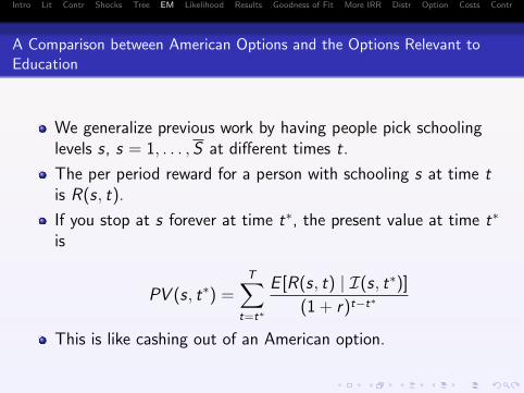
A Comparison between American Options and the Options Relevant toEducation
We generalize previous work by having people pick schoolinglevels s, s = 1, . . . , S at different times t.
The per period reward for a person with schooling s at time tis R(s, t).
If you stop at s forever at time t∗, the present value at time t∗
is
PV (s, t∗) =T∑
t=t∗
E [R(s, t) | I(s, t∗)]
(1 + r)t−t∗
This is like cashing out of an American option.

Intro Lit Contr Shocks Tree EM Likelihood Results Goodness of Fit More IRR Distr Option Costs Contr
If you stop at s at time t∗, and then go on to s ′ the nextperiod, the return evaluated at time t at state s ′ is
R(s, t∗) +1
1 + rE [V (s ′, t + 1) | I(s, t)].
Similarly, there is the strategy that has the agent stay on at sfor two periods then moves, etc.
R(s, t∗) +E [R(s, t∗ + 1) | I(s, t∗)]
1 + r
+1
(1 + r)2E [V (s ′, t∗ + 2) | I(s, t∗)].
Intro Lit Contr Shocks Tree EM Likelihood Results Goodness of Fit More IRR Distr Option Costs Contr
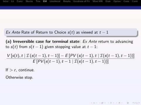
Ex Ante Rate of Return to Choice s(t) as viewed at t − 1
(a) Irreversible case for terminal state: Ex Ante return to advancingto s(t) from s(t − 1) given stopping value at t − 1:
V [s(t), t | I (s(t − 1), t − 1)]− E [PV (s(t − 1), t | I(s(t − 1), t − 1))]
E [PV (s(t − 1), t − 1 | I(s(t − 1), t − 1))]
If > r , continue.
Otherwise stop.
Intro Lit Contr Shocks Tree EM Likelihood Results Goodness of Fit More IRR Distr Option Costs Contr
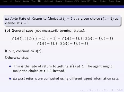
Ex Ante Rate of Return to Choice s(t) = s at t given choice s(t − 1) asviewed at t − 1
(b) General case (not necessarily terminal states):
V (s(t), t | I(s(t − 1), t − 1)− V (s(t − 1), t | I(s(t − 1), t − 1)
V (s(t − 1), t | I(s(t − 1), t − 1)
If > r , continue to s(t).
Otherwise stop.
This is the rate of return to getting s(t) at t. The agent mightmake the choice at t + 1 instead.
Ex post returns are computed using different agent information sets.

Intro Lit Contr Shocks Tree EM Likelihood Results Goodness of Fit More IRR Distr Option Costs Contr
In Summary, in Our Model
Two distinct concepts.
(i) Ever making the choice(ii) Making the choice at t
The traditional approach (Becker-Mincer) assumes schoolingdecisions are made at fixed ages and are irreversible.
Compares two streams only
Our evidence shows the opposite is true. A lot of fluidity —delay, dropping in and out.

Intro Lit Contr Shocks Tree EM Likelihood Results Goodness of Fit More IRR Distr Option Costs Contr
Ingredients
Econometric Model
We postulate a factor structure for arrival of information.
Let Θ be set of factors.
Agents update information using the factor structure.
Occupying a state can reveal a factor.

Intro Lit Contr Shocks Tree EM Likelihood Results Goodness of Fit More IRR Distr Option Costs Contr
Ingredients
Model’s Ingredients
Earnings:
Yi (s, t, θ) = αt(s) + βt(s)θi + εYt,i (s) for s ∈ S
where εYt,i (s) ⊥⊥ θi ,∀t, and εYt,i (s) ⊥⊥ εYt′,i ′(s)∀t, t ′, i , i ′
Schooling Costs: Cost of going from s(t) to s(t + 1)
Ci (s(t), s(t + 1), t, θ) = λt(s(t), s(t + 1)) + λθt (s(t), s(t + 1))θi
+ εCt,i (s(t), s(t + 1))
where εCt,i (s(t), s(t + 1)) ⊥⊥ θi ,εCt,i (s(t), s(t + 1)) ⊥⊥ εCt′,i ′(s(t), s(t + 1)) for any t, t ′ (t 6= t ′ forindividual i) and individuals i , i ′.

Intro Lit Contr Shocks Tree EM Likelihood Results Goodness of Fit More IRR Distr Option Costs Contr
Ingredients
Model Ingredients
In a data set with truncated earnings histories due to upperlimits on the length of panels, the estimated “cost” is true costminus the discounted earnings history after truncation.
Model is identified using the analysis of Abbring and Heckman(2007) and Heckman and Navarro (2007).
Identification and interpretation of the factor structure modelsare facilitated by test score equations.

Intro Lit Contr Shocks Tree EM Likelihood Results Goodness of Fit More IRR Distr Option Costs Contr
Ingredients
Model’s Ingredients
Measurement System: For agent i the test score j is:
Ti(j , θ) = π(j) + πTθ (j)θi + ei(j)
where ei(j) ⊥⊥ θ, and e ′i (j′) ⊥⊥ ei(j).
Test scores include cognitive and non-cognitive terms.
Test Score: Arithmetic Reasoning, Word Knowledge, ParagraphComprehension, Mathematical Knowledge, NumericalOperations, Coding Speed, Rotter Locus of Control Scale,Rosenberg Self-Esteem Scale.

Intro Lit Contr Shocks Tree EM Likelihood Results Goodness of Fit More IRR Distr Option Costs Contr
Ingredients
Model’s Ingredients
Relies on “full support” conditions (identification at infinity)which we check.
Information updating:
1 Agents know the X .2 They know the parameters including factor loadings in cost
and outcome equations.3 They learn about the e (ex ante set to zero).4 They learn about components of θ which arrive when states
are experienced (ex ante expected θ are zero).

Intro Lit Contr Shocks Tree EM Likelihood Results Goodness of Fit More IRR Distr Option Costs Contr
Solution: Backward Induction
There are terminal states and solve by backward induction.
Intro Lit Contr Shocks Tree EM Likelihood Results Goodness of Fit More IRR Distr Option Costs Contr
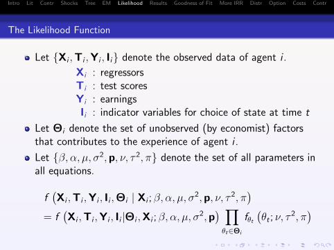
The Likelihood Function
Let {Xi ,Ti ,Yi , Ii} denote the observed data of agent i .
Xi : regressorsTi : test scoresYi : earningsIi : indicator variables for choice of state at time t
Let Θi denote the set of unobserved (by economist) factorsthat contributes to the experience of agent i .
Let {β, α, µ, σ2,p, ν, τ 2, π} denote the set of all parameters inall equations.
f(Xi ,Ti ,Yi , Ii ,Θi | Xi ; β, α, µ, σ
2,p, ν, τ 2, π)
= f(Xi ,Ti ,Yi , Ii |Θi ,Xi ; β, α, µ, σ
2,p) ∏θt∈Θi
fθt(θt ; ν, τ
2, π)
Intro Lit Contr Shocks Tree EM Likelihood Results Goodness of Fit More IRR Distr Option Costs Contr
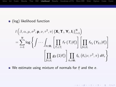
(log) likelihood function
l(β, α, µ, σ2,p, ν, τ 2, π| {Xi ,Ti ,Yi , Ii}Ni=1
)=
N∑i=1
log
{∫· · ·∫θ∈Θi
[∏Ti∈Ti
fT (Ti |θ′i)
][∏S∈Si
fYS(YS,i |θ′i)
][∏
S∈Si
gS (1|θ′i)
] ∏θt∈Θi
fθr(θr |ν, τ 2, π
)dθr
}
We estimate using mixture of normals for θ˜ and the e.
Intro Lit Contr Shocks Tree EM Likelihood Results Goodness of Fit More IRR Distr Option Costs Contr
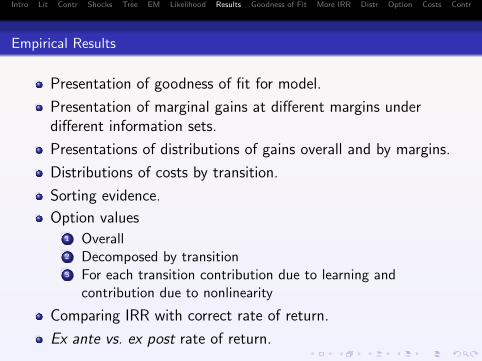
Empirical Results
Presentation of goodness of fit for model.
Presentation of marginal gains at different margins underdifferent information sets.
Presentations of distributions of gains overall and by margins.
Distributions of costs by transition.
Sorting evidence.
Option values1 Overall2 Decomposed by transition3 For each transition contribution due to learning and
contribution due to nonlinearity
Comparing IRR with correct rate of return.
Ex ante vs. ex post rate of return.

Intro Lit Contr Shocks Tree EM Likelihood Results Goodness of Fit More IRR Distr Option Costs Contr
Goodness of Fit

Intro Lit Contr Shocks Tree EM Likelihood Results Goodness of Fit More IRR Distr Option Costs Contr
The Data
NLSY
Some background statistics on the evolution of schooling.

Intro Lit Contr Shocks Tree EM Likelihood Results Goodness of Fit More IRR Distr Option Costs Contr
0
20
40
60
80
100
Perc
enta
ge
14s1
17s2
18s2
19s1
19s2
20s1
20s2
21s2
22s2
23s2
24s2
Note: .
NLSY79 − Sample of White Males
Figure 1. Evolution of Schooling Attainment
Enrolled in HS HS Dropouts HS Graduates GEDs
GED+Some College Enrolled in College Some 2YC (Not Enrolled) Some 4YC (Not Enrolled)
AA Degree BA/BS Degree

Intro Lit Contr Shocks Tree EM Likelihood Results Goodness of Fit More IRR Distr Option Costs Contr
0
20
40
60
80
100
Perc
enta
ge
14s1
17s2
18s2
19s1
19s2
20s1
20s2
21s2
22s2
23s2
24s2
Note: .
NLSY79 − Simulated Sample
Figure 2. Evolution of Schooling Attainment
Enrolled in HS HS Dropouts HS Graduates GEDs
GED+Some College Enrolled in College Some 2YC (Not Enrolled) Some 4YC (Not Enrolled)
AA Degree BA/BS Degree

Intro Lit Contr Shocks Tree EM Likelihood Results Goodness of Fit More IRR Distr Option Costs Contr
GED
Paths to the GEDActual and Simulated Data
EHSActualSimul.
EHS89.4%89.6 %
EHS24.8%24.6%
HSD36.7%34.3%
GED30.2%35.5%
HSD69.8%64.5%
HSD10.6%10.4%
GED10.2%12.2%
GED
HSD89.8%87.8%
GED9.2%11.2%
GED
HSD90.8%88.8%
GED24.4%25.0%
HSD75.6%75.0%
Age 14 Age 17 Age 18 Age 20 Age 22 Age 34
EHS = Enrolled in High SchoolHSD = High School DropoutGED = GED Recipient
1

Intro Lit Contr Shocks Tree EM Likelihood Results Goodness of Fit More IRR Distr Option Costs Contr
GED
Traditional Rates of Return and the Model Estimated Rate ofReturn (Including Option Value Incentives)

Intro Lit Contr Shocks Tree EM Likelihood Results Goodness of Fit More IRR Distr Option Costs Contr
GED
Earnings per Age/Semester Ever High School Graduates versus EverFour Year College Graduates Model versus Data
Earnings per Age/SemesterEver High School Graduates versus Ever Four Year College Graduates
Model versus Data
0
5
10
15
20
25
30
18s1
18s2
19s1
19s2
20s1
20s2
21s1
21s2
22s1
22s2
23s1
23s2
24s1
24s2 s5s
125
s226
s126
s227
s127
s228
s128
s229
s129
s230
s130
s231
s131
s232
s132
s233
s133
s234
s134
s235
s135
s236
s1
Age/Semester
Thou
sand
s of D
ollar
s
High School Graduates Data Four Year College Graduates DataHigh School Graduates Model Four Year College Graduates Model

Intro Lit Contr Shocks Tree EM Likelihood Results Goodness of Fit More IRR Distr Option Costs Contr
GED
Present Discounted Value of Earnings, Rate of Returns and InternalRate of Returns High School Graduates versus Four Year CollegeGraduates
High School Four Year High School Four YearGraduates College Grad Graduates College Grad
Present Value of Earnings (a) 379.994 459.014 377.188 450.795Rate of ReturnIRRMincer Coefficient (Age 30)Note: (a) We assume an annual discount rate of 3%.
9.45% 8.9%
20.8%9%
19.5%9%
PV of Earnings, Rate of Returns, Mincer Coefficient and Internal Rate of ReturnsHigh School Graduates versus Four Year College Graduates
Data Model

Given High School Enrollment at Age 18 — Top of TreeFigure 1. Evolution of Education AchievedNLSY79 - White Males
14s1 17s1 18s2 19s1 – 24s2 26s2
EHS (1954)
HSD (210)
HSD (188)
HSD (172)
HSD (156) HSD (156) HSD (156)
GED (16)
GED (11) GED (11)
ECO (5) COL (5)
GED (16)
GED (11) GED (11) GED (11)
ECO (5) COL (5) COL (5)
GED (22)
GED (9) GED (9) GED (9) GED (9)
ECO (13) COL (13) COL (13) COL (13)
EHS (1744)
EHS (433)
HSD (159)
HSD (111) HSD (111) HSD (111)
GED (48)
GED (33) GED (33)
ECO (15) COG (15)
HSG (274)
HSG (163) HSG (163) HSG (163)
ECO (111)
SCO (98) SCO (98)
COG (13) COG (13)
HSG (1311)
HSG (579)
HSG (437) HSG (437) HSG (437)
ECO (142)
SCO (103) SCO (103)
COG (39) COG (39)
ECO (732)
SCO (171) SCO (171) SCO (171)
COG (561) COG (561) COG (561)
14s1 17s1 18s2 20s2 22s2 24s2 26s2
EHS = Enrolled in High School HSG = High School GraduateHSD = High School Dropout ECO = Enrolled in CollegeSCO = Some College Completed GED = GED Completed
Note: All figures are in 2000 US Dollars.
1

Intro Lit Contr Shocks Tree EM Likelihood Results Goodness of Fit More IRR Distr Option Costs Contr
Present Discounted Value of Earnings, Rate of Returns and InternalRate of Returns High School Graduates versus Four Year CollegeGraduates
High School Four Year High School Four Year High School Four YearGraduates College Grad Graduates College Grad Graduates College Grad
Present Value of Earnings (a) 377.188 450.795 394.413 509.991 482.037 551.627Rate of ReturnIRR
Note: (a) We assume an annual discount rate of 3%.
29.3%19.5%11%9%
Four Year Ever Four Year
Present Discounted Value of Earnings, Rate of Returns and Internal Rate of ReturnsHigh School Graduates versus Four Year College Graduates
Ever Four Year
14.4%6%
College Grad. College Grad. On Time College Grad. - Top Cognitive Ability

Intro Lit Contr Shocks Tree EM Likelihood Results Goodness of Fit More IRR Distr Option Costs Contr
Earning Profiles for High School Graduates at Age 18 Ever FourYear College Grad. Versus High School Grad. Top Decile ofCognitive Ability (fC > dC
10).Earning Profiles for High School Graduates at Age 18
Ever Four Year College Grad. Versus High School Grad.Top Decile of Cognitive Ability (fC>d10
C)
0
5
10
15
20
25
30
35
40
18s2 19s1 19s2 21s1 22s2 24s2 26s2 28s2 30s2 32s2 34s2
Age/Semester
Thou
sand
s of D
ollar
s
College Grad. High School Grad.

Intro Lit Contr Shocks Tree EM Likelihood Results Goodness of Fit More IRR Distr Option Costs Contr
Estimated Distributions of Abilities
First, overall distributions.
Evidence on sorting by ability type.

Intro Lit Contr Shocks Tree EM Likelihood Results Goodness of Fit More IRR Distr Option Costs Contr
0.2
.4.6
.81
Fact
or
−3 −2 −1 0 1 2Density
Four Year College Some Four Year College Two Year College Some Two Year College
High School Graduate GED with Some College GED High School Dropout
Note:
NLSY79 − Sample of White Males
Figure 1. Distribution of Cognitive FactorBy Final Schooling Level (overall)

Intro Lit Contr Shocks Tree EM Likelihood Results Goodness of Fit More IRR Distr Option Costs Contr
0.2
.4.6
.81
Fact
or
−2 −1 0 1 2Density
Four Year College Some Four Year College Two Year College Some Two Year College
High School Graduate GED with Some College GED High School Dropout
Note:
NLSY79 − Sample of White Males
Figure 2. Distribution of Non−Cognitive FactorBy Final Schooling Level (overall)

Intro Lit Contr Shocks Tree EM Likelihood Results Goodness of Fit More IRR Distr Option Costs Contr
1 2 3 4 5 6 7 8 9 100
0.1
0.2
0.3
0.4
0.5
0.6
0.7
0.8
0.9
1Schooling Levels by Decile of Cognitive Ability
Decile
Frac
tion
4-YCollege Some 4-YCollege 2-YCollege Some 2-YCollege GED with Some College HS Diploma GED HS Dropout

Intro Lit Contr Shocks Tree EM Likelihood Results Goodness of Fit More IRR Distr Option Costs Contr
1 2 3 4 5 6 7 8 9 100
0.1
0.2
0.3
0.4
0.5
0.6
0.7
0.8
0.9
1Schooling Levels by Decile of Personality Trait
Decile
Frac
tion
4-YCollege Some 4-YCollege 2-YCollege Some 2-YCollege GED with Some College HS Diploma GED HS Dropout

Intro Lit Contr Shocks Tree EM Likelihood Results Goodness of Fit More IRR Distr Option Costs Contr
0.2
.4.6
.81
Fact
or
−3 −2 −1 0 1 2Density
High School Dropout Late HSD, Late GED Early HSD, Early GED Early HSD, GED
Early HSD, Late GED GED with Some College
Note:
NLSY79 − Sample of White Males
Figure 3. Distribution of Cognitive FactorBy Final Schooling Level: HSD, GED, GED with Some College

Intro Lit Contr Shocks Tree EM Likelihood Results Goodness of Fit More IRR Distr Option Costs Contr
0.2
.4.6
.81
Fact
or
−2 −1 0 1 2Density
High School Dropout Late HSD, Late GED Early HSD, Early GED Early HSD, GED
Early HSD, Late GED GED with Some College
Note:
NLSY79 − Sample of White Males
Figure 4. Distribution of Non−Cognitive FactorBy Final Schooling Level: HSD, GED, GED with Some College

Intro Lit Contr Shocks Tree EM Likelihood Results Goodness of Fit More IRR Distr Option Costs Contr
Schooling
Sorting of People into Schools Based on Cognitive and NoncognitiveAbilities

Intro Lit Contr Shocks Tree EM Likelihood Results Goodness of Fit More IRR Distr Option Costs Contr
Schooling
A. Enrolled in High School at Age 17 B. High School Dropout at Age 17
Distribution of Unobserved Abilities by Schooling Level at Age 17: Transition from "Enrolled in HS" (Age 14) to "Enrolled in HS" or "HS Dropout"
Cognitive Cognitive Noncognitive Noncognitive
Note: We use the convention that decile 1 enters the lowest ability levels,whereas decile 10 contains the highest ability levels. The levels are computedusing the overall distribution.

Intro Lit Contr Shocks Tree EM Likelihood Results Goodness of Fit More IRR Distr Option Costs Contr
Schooling
Distribution of Unobserved Abilities: Transition from "High School Graduate at Age 18" to "College Enrollment at Age 19" or "High School Graduate at Age 19"
A. Hich School Graduates at Age 18
B1. College Enrollment at Age 19 B2. High School Graduates at Age 19
CognitiveNoncognitive
CognitiveCognitive NoncognitiveNoncognitive
Intro Lit Contr Shocks Tree EM Likelihood Results Goodness of Fit More IRR Distr Option Costs Contr
Schooling
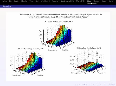
Distribution of Unobserved Abilities: Transition from "Enrolled in a Four Year College at Age 19/2st Sem." to "Four Year College Graduate at Age 22" or "Some Four Year College at Age 22"
A. Enrolled in a Four Year College at Age 19
B1. Four Year College Grad. at Age 22 B2. Some Four Year College at Age 22CognitiveNoncognitive
CognitiveCognitive
NoncognitiveNoncognitive

Intro Lit Contr Shocks Tree EM Likelihood Results Goodness of Fit More IRR Distr Option Costs Contr
Schooling
Distribution of Unobserved Abilities: Transition from "High School Graduate at Age 19/HS Diploma at Age 18" to "Enrolled in College at Age 20" or "High School Graduate at Age 20"
A. High School Grad. at Age 19
B1. Enrolled in College at Age 20 B2. High School Grad. at Age 20Cognitive
CognitiveCognitiveNoncognitiveNoncognitive
Noncognitive

Intro Lit Contr Shocks Tree EM Likelihood Results Goodness of Fit More IRR Distr Option Costs Contr
Schooling
Distribution of Unobserved Abilities: Transition from "Enrolled in Four Year College at Age 20/2nd Sem. / HS Diploma at Age 18" to "Four Year College Grad. at Age 23" or "Some Four Year College at Age 23"
A. Enrolled in Four Year College at Age 20
B1. Four Year College Grad. at Age 23 B2. Some Four Year College at Age 23
Cognitive
Cognitive
Cognitive NoncognitiveNoncognitive
Noncognitive
Intro Lit Contr Shocks Tree EM Likelihood Results Goodness of Fit More IRR Distr Option Costs Contr
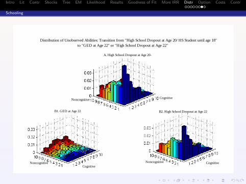
Schooling
Distribution of Unobserved Abilities: Transition from "High School Dropout at Age 20/HS Student until age 18" to "GED at Age 22" or "High School Dropout at Age 22"
A. High School Dropout at Age 20-
B1. GED at Age 22 B2. High School Dropout at Age 22
CognitiveNoncognitive
CognitiveCognitive
NoncognitiveNoncognitive
Intro Lit Contr Shocks Tree EM Likelihood Results Goodness of Fit More IRR Distr Option Costs Contr
Schooling
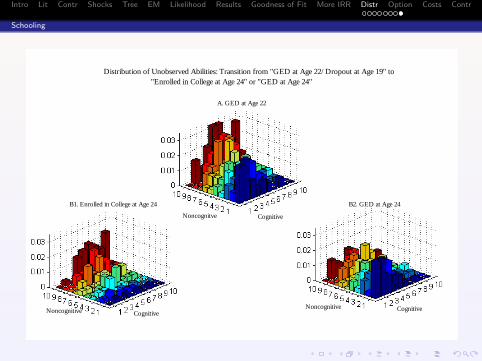
Distribution of Unobserved Abilities: Transition from "GED at Age 22/Dropout at Age 19" to "Enrolled in College at Age 24" or "GED at Age 24"
A. GED at Age 22
B1. Enrolled in College at Age 24 B2. GED at Age 24
Cognitive
CognitiveCognitive
Noncognitive
Noncognitve
Noncognitive

Intro Lit Contr Shocks Tree EM Likelihood Results Goodness of Fit More IRR Distr Option Costs Contr
Option Values of Various Educational States
Consider estimating the option value of the GED as part of ageneral project to estimate the option value of different typesof schooling and training.
A stochastic dynamic programming model with informationupdating.
A few people benefit. Most do not.

Intro Lit Contr Shocks Tree EM Likelihood Results Goodness of Fit More IRR Distr Option Costs Contr
First consider option values for enrollment in a state at one agecompared to another state at that age.
We later consider the value of having the option whenever it isused.

Distribution of Option Values - Early GED
0.1
.2.3
.4D
ensit
y
0 2 4 6 8Thousands of Dollars
Note: Source Heckman and Urzua (2008).
Early High School Dropouts (age 17) - Sample of White Males
Distribution of Option Values - Early GED
Pr(Option Value<$220)=5% Pr(Option Value<$400)=10%Pr(Option Value<$846)=25% Pr(Option Value<$1,620)=50%Pr(Option Value<$2,800)=75%

Intro Lit Contr Shocks Tree EM Likelihood Results Goodness of Fit More IRR Distr Option Costs Contr

Intro Lit Contr Shocks Tree EM Likelihood Results Goodness of Fit More IRR Distr Option Costs Contr
0.2
.4.6
Opt
ion
Val
ue
0 2 4 6Thousands of Dollars
Note: Source Heckman and Urzua (2008).
For High School Dropouts at Age 18 who dropped out by Age 17 − White Males
Distribution of Option Values Associated with GED at Age 20
Pr(Option Value<$123)=5% Pr(Option Value<$225)=10%Pr(Option Value<$480)=25% Pr(Option Value<$941)=50%Pr(Option Value<$1,735)=75%
21

Intro Lit Contr Shocks Tree EM Likelihood Results Goodness of Fit More IRR Distr Option Costs Contr
For High School Dropouts at Age 18 who dropped out by Age 17 − White Males Average Option Value Associated with GED at Age 20, by Deciles of Ability Levels
Cognitive
Noncognitive
22
Intro Lit Contr Shocks Tree EM Likelihood Results Goodness of Fit More IRR Distr Option Costs Contr
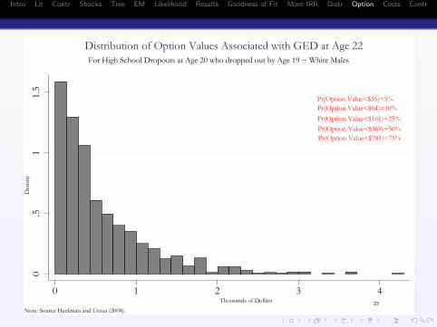
0.5
11.
5D
ensit
y
0 1 2 3 4Thousands of Dollars
Note: Source Heckman and Urzua (2008).
For High School Dropouts at Age 20 who dropped out by Age 19 − White Males
Distribution of Option Values Associated with GED at Age 22
Pr(Option Value<$35)=5% Pr(Option Value<$64)=10%Pr(Option Value<$161)=25% Pr(Option Value<$369)=50%Pr(Option Value<$781)=75%
23

Intro Lit Contr Shocks Tree EM Likelihood Results Goodness of Fit More IRR Distr Option Costs Contr
0.5
11.
52
2.5
Den
sity
0 .5 1 1.5 2 2.5Thousands of Dollars
Note: Source Heckman and Urzua (2008).
For High School Dropouts at Age 20 who dropped out by Age 17 − White Males
Distribution of Option Values Associated with GED at Age 22
Pr(Option Value<$89)=10%Pr(Option Value<$105)=25%Pr(Option Value<$228)=50%
25

Intro Lit Contr Shocks Tree EM Likelihood Results Goodness of Fit More IRR Distr Option Costs Contr
Simulation Exercise: The Effects of Eliminating the GEDa
aNote: The numbers in columns (1) and (2) are computed as fractions ofthe overall population.
Schooling Level Simulated No GED Change in Rate % Change (1) (2) (2)-(1) ((2)/(1) - 1)%
Four Year College 26.4% 28.0% 1.6% 6.1%Some Four Year College 7.0% 7.8% 0.8% 11.4%Two Year College 5.8% 6.3% 0.5% 8.5%Some Two Year College 9.3% 9.8% 0.5% 5.0%Some College GED 2.9% - - -High School Graduates 32.8% 35.0% 2.1% 6.5%GEDs 3.6% - - -High School Dropouts 12.1% 13.1% 1.0% 8.4%
Simulation Exercise: The Effects of Eliminating the GED (a)
Note: (a) The numbers in columns (1) and (2) are computed as fractions of the overall population.

Intro Lit Contr Shocks Tree EM Likelihood Results Goodness of Fit More IRR Distr Option Costs Contr
Decompose: High School vs. College (enrollment)
(a) Option values by contribution from each transition.
(b) Sources: learning and nonlinearity.
(c) True Rate of return by age and by transition (perceived atdifferent ages and transitions).

Intro Lit Contr Shocks Tree EM Likelihood Results Goodness of Fit More IRR Distr Option Costs Contr
Option Value and Its Decomposition UnconditionalfC<d1
C fC>d10C fN<d1
N fN>d10N fC<d1
C fC>d10C
fN<d1N fN>d10
N
Overall Option Value Associated with College Enrollment=(1)+(2)+(3)+(4) 27,474 6,574 61,179 12,903 90,045 1,297 171,680Decomposition:
(1) College Enrollment at Age 19 (on time) 16,604 395 50,036 11,683 27,151 659 77,486after Graduating from HS at Age 18 (on time) (b)
(2) College Enrollment at Age 20 (delayed) 5,390 1,490 7,244 960 24,185 271 55,900after Graduating from HS at Age 18 (on time)
(3) College Enrollment at Age 20 (delayed) 5,452 4,685 3,869 223 38,696 353 38,264after Graduating from HS at Age 19 (delayed)
(4) College Enrollement at Age 24 28 4 30 37 13 14 30after dropping out from HS at Age 19 and
obtaining GED at age 22
Notes: (a) All the numbers are in thousands of dollars at age 17; (b) In this case the option value is generated imposing that the agent cannot go back to college in thefuture. The option value associated with this possibility is presented in (2); (c ) dj
k denotes the j-th decile associated with factor k. The deciles are computed from the overalldistributions of abilities.
The Option Value of College EnrollmentHigh School Students at Age 17 (a)
Dynamic Schooling Model with Learning (I ={fC,fN,θ} )
Cognitive Ability ( c) Noncognitive Ability ( c) Both Abilities ( c)

Intro Lit Contr Shocks Tree EM Likelihood Results Goodness of Fit More IRR Distr Option Costs Contr
Option Value and Its Decomposition Learning No Learning DifferenceI={fC,fN,θ} I={fC,fN}
Overall Option Value Associated with College Enrollment=(1)+(2)+(3)+(4) 27,474 14,408 13,066Decomposition:
(1) College Enrollment at Age 19 (on time) 16,604 8,861 7,743after Graduating from HS at Age 18 (on time) (b)
(2) College Enrollment at Age 20 (delayed) 5,390 1,745 3,645after Graduating from HS at Age 18 (on time)
(3) College Enrollment at Age 20 (delayed) 5,452 3,784 1,668after Graduating from HS at Age 19 (delayed)
(4) College Enrollement at Age 24 28 18 10after dropping out from HS at Age 19 and
obtaining GED at age 22
Notes: (a) All the numbers are in thousands of dollars at age 17. The sample is unchanged across simulations, that is, thenumbers are computed for those agents enrolled in high school at age 17 under the three factor model.; (b) In this case theoption value is generated imposing that the agent cannot go back to college in the future. The option value associated withthis possibility is presented in (2).
The Contribution of Learning to the Option Value of College EnrollmentHigh School Students at Age 17 (a)
Dynamic Schooling Model with Learning vs. without Learning

Intro Lit Contr Shocks Tree EM Likelihood Results Goodness of Fit More IRR Distr Option Costs Contr
Initial State Average Treatment Treament on Treatment on theEffect the Treated Untreated
(1) High School Grad. At Age 18Ever 4.80% 18.27% -12.20%
Once for All 12.60% 20.25% 2.90%(2) High School Grad. At Age 19 -51.30% 160% -127%
Grad. High School at Age 18(3) High School Grad. At Age 19 45.05% 487% -175%
Enrolled in HS at Age 18
(1) High School Grad. At Age 18Ever -2.92% 9.06% -9.02%
Once for All -2.72% 9.64% -9.01%(2) High School Grad. At Age 19 -111.90% 38% -125.20%
Grad. High School at Age 18(3) High School Grad. At Age 19 -118.80% 36.40% -136.20%
Enrolled in HS at Age 18
(1) High School Grad. At Age 18Ever 7.14% 20.52% -13.57%
Once for All 20.12% 23.32% 15.17%(2) High School Grad. At Age 19 -6.65% 183.20% -117.50%
Grad. High School at Age 18(3) High School Grad. At Age 19 221.10% 566.50% -138.40%
Enrolled in HS at Age 18
Low Ability Individuals (fC<d5C and fN<d5
N)
High Ability Individuals (fC>d4C and fN>d4
N)
Unconditional
High School Grad. versus. College EnrollmentTrue Rate of Return

Intro Lit Contr Shocks Tree EM Likelihood Results Goodness of Fit More IRR Distr Option Costs Contr
Costs

Intro Lit Contr Shocks Tree EM Likelihood Results Goodness of Fit More IRR Distr Option Costs Contr
0.0
02.0
04.0
06.0
08.0
1
−300 −200 −100 0 100
Note: Source Heckman and Urzua (2008).
Distribution of Costs: Transition from "High School Dropout at Age 17" to "GED at Age 18"
Thousands of Dollars

Intro Lit Contr Shocks Tree EM Likelihood Results Goodness of Fit More IRR Distr Option Costs Contr
0.0
02.0
04.0
06.0
08.0
1
−150 −100 −50 0 50 100
Note: Source Heckman and Urzua (2008).
Distribution of Costs: Transition from "High School Dropout at Age 20/HS student until Age 19" to "GED at Age 22"
Thousands of Dollars

Intro Lit Contr Shocks Tree EM Likelihood Results Goodness of Fit More IRR Distr Option Costs Contr
0.0
05.0
1.0
15
150 100 50 0 50
Note: Source Heckman and Urzua (2008).
Distribution of Costs: Transition from "High School Dropout at Age 22/HS dropout at Age 17" to "GED at Age 22"
Thousands of Dollars

Intro Lit Contr Shocks Tree EM Likelihood Results Goodness of Fit More IRR Distr Option Costs Contr
Support Conditions Satisfied?

Intro Lit Contr Shocks Tree EM Likelihood Results Goodness of Fit More IRR Distr Option Costs Contr
Figure. Support Conditions for the Analysis of High School Graduation
A. Overall Sample
0.5
11.
52
2.5
33.
54
Freq
uenc
y
0 .2 .4 .6 .8 1Probability of Graduating from High School
B. Sample of High School Graduates C. Sample of High School Dropouts
0.5
11.
52
2.5
33.
54
Freq
uenc
y
.2 .4 .6 .8 1Probability of Graduating from High School
0.5
11.
52
2.5
33.
54
Freq
uenc
y
0 .2 .4 .6 .8 1Probability of Graduating from High School
Notes: Each panel presents the distribution of the probability of graduating from high school. This probability isestimated from the structural model, and consequently, it is estimated taking into the account the dynamic schoolingdecisions as well as unoberserved heterogeneity.

Intro Lit Contr Shocks Tree EM Likelihood Results Goodness of Fit More IRR Distr Option Costs Contr
Summary
We develop a model of educational choices with uncertainty,learning about serially correlated shocks, dropout and delay.
We consider high school, dropout, GED and college choicesjointly.
We generalize the rate of return and show the inadequacy ofthe IRR and rates of return in this more general setting.
Option values are computed by stage and due to nonlinearityand uncertainty.
Ex ante/ex post distinctions are substantial.
They are substantial and raise the rate of return substantiallybeyond traditional measures.

Intro Lit Contr Shocks Tree EM Likelihood Results Goodness of Fit More IRR Distr Option Costs Contr
Theoretical Contributions of this Paper
A dynamic sequential model of educational choices amongdiscrete states with option values arising from learning andnonlinearity of reward functions at different stages of the lifecycle.
We build a model of schooling connecting high school droppingout, GED attainment, delay, college choices and returns.
Define the correct concept of the rate of return to schooling ina dynamic model with uncertainty, nonlinearity and delay.
Builds on previous work on dynamic selection into schooling(Altonji, 1993; Keane and Wolpin, 1997, 2001; Eckstein andWolpin, 1999; Arcidiacono, 2004; Cameron and Heckman,1998, 2001).
Like Arcidiacono (2004), we model learning about persistentshocks (see also Miller, 1984; Pakes, 1986; and others).

Intro Lit Contr Shocks Tree EM Likelihood Results Goodness of Fit More IRR Distr Option Costs Contr
Agents are risk neutral.
Our model is identified semiparametrically:
(i) non-parametric identification of distributions of unobservablesthat are serially persistent;
(ii) earnings equations parametric (but flexible functional forms).

Intro Lit Contr Shocks Tree EM Likelihood Results Goodness of Fit More IRR Distr Option Costs Contr
Empirical Contributions of This Paper
Estimate true rates of return and compare with IRR.
Decompose option values by stages (educational choices andtimes choices are made; account for delay).
Estimate at each stage the respective contributions ofnon-linearity and learning to option values and rates of return.
Estimate contributions of both cognitive and noncognitive skillsto returns and costs.
We analyze jointly high school dropout and GED returns, aswell as returns to two year and four year colleges(Eckstein-Wolpin, 1999).
Schooling states s need not be ordered.