Embed Size (px)
Citation preview

THE OPERATION PLATFORM RECOMMENDATION FOR THE
DEREGULATED UTILITY INDUSTRY IN THAILAND
by
CHAI CHOMPOO-INWAI
Presented to the Faculty of the Graduate School of
The University of Texas at Arlington in Partial Fulfillment
of the Requirements
for the Degree of
DOCTOR OF PHILOSOPHY
THE UNIVERSITY OF TEXAS AT ARLINGTON
August 2005

ACKNOWLEDGEMENTS
Sincere appreciation is expressed to Dr.Wei-Jen Lee, Dr. Raymond R. Shoults,
Dr. William E. Dillon, Dr. Kai Yeung, and Dr. Atilla Dogan for their guidance as
members of the author’s graduate committee, in particularly to the author’s supervising
professor, Dr. Wei-Jen Lee for his full advice, full support, and full encouragement
throughout the time of the author’s graduate study.
The author would also want to express appreciation to all members of Energy
System Research Center, ESRC, The University of Texas at Arlington for all their
valuable assistances, discussions, and enjoyable association. Besides, a special gratitude
is reserved for all my friends from the Thai Student Association. Their careful review,
helpful suggestions and discussions in this dissertation are sincerely appreciated.
Furthermore, the author would like to thank the Energy Policy and Planning
Organization, EPPO for fully granting the author the time required for his PH.D., and a
further thank you to Electricity Generating Authority of Thailand, EGAT for providing
system data.
Finally, the author is most grateful to his family: his father, Mr. Prasit, his
mother Mrs. Junsom, and his brother Mr. Chow for their full support, patience, and
understanding during my graduate academic period.
May 8, 2005
ii
ABSTRACT
THE OPERATION PLATFORM RECOMMENDATION OF THE
DEREGULATED UTILITY INDUSTRY IN THAILAND
Publication No. ______
Chai Chompoo-inwai, PhD.
The University of Texas at Arlington, 2005
Supervising Professor: Dr. Wei-Jen Lee
Transmission Congestion Management (TCM) plays a significant role in power
system operation under today deregulated environment. It has two major functions of an
apparatus to keep power system running within acceptable security limits, and of a tool
allocating financial obligation to market participants then paying back to transmission
grid investors. TCM issue has been widely debating during a past decade, until now, it
is still an opened issue extensively discussed in the current structure of competitive
environment.
In the United State, there are existing two successful stories of TCM under
different operation schemes, the former is PJM with Nodal Congestion Management
(NCM) based on the renowned Location Marginal Price (LMP), while the latter is Zonal iii

Congestion Management (ZCM) deploying in Electricity Reliability Council of Texas
(ERCOT). Though PJM model is adopted in some developing countries where the
processes of restructuring of Electricity Supply Industry (ESI) is still under the
beginning phase, many concerns such as: advance in an information technology, energy
security, social equity, price volatility, and the need to subsidize the poor consumers,
are necessary to be considered before the establishment of TCM and settlement
processes.
Thailand is a developing country located in the heart of South-east Asia, and
now being on the processes of transformation in ESI structure. Although the first
initiation in this issue has been discussed since 1999 by government and related
agencies, however, there is still unclear direction for the new reforming paradigm.
Taking into account all above concerns, together with the studying of Transmission
Congestion Management Techniques, Power System Security, and System wide
economic benefit, this dissertation proposes a recommendation platform of the
deregulated utility industry in Thailand during its transformation stage in order to have
a smooth transition moving from the traditional vertically integrated system to a new
competitive environment.
iv
TABLE OF CONTENTS
ACKNOWLEDGEMENTS....................................................................................... ii ABSTRACT .............................................................................................................. iii LIST OF ILLUSTRATIONS..................................................................................... xi LIST OF TABLES..................................................................................................... xiii Chapter 1. INTRODUCTION………. ............................................................................ 1 1.1 Background and emerging problems ....................................................... 1 1.2 Chronology of events in Electricity Supply Industry .............................. 3 1.3 Survey of literatures……......................................................................... 5 1.4 Motivations, Objectives, and Approaches ............................................... 12 1.5 Synopsis of chapters ............................................................................... 16
2. TRANSMISSION CONGESTION MANAGEMENT ................................. 18 2.1 Introduction and problem in Regulatory System .................................... 18 2.2 Power system operation in Competitive Environment ............................ 19 2.3 Congestion Management process and two settlement system................. 21 2.4 Market-based Congestion Management .................................................. 23 2.4.1 Centralized approach based on Locational Marginal Pricing……. ........................................... 23 2.4.2 Decentralized approach based on Zonal Pricing ...................... 24 v

2.5 Zonal Congestion Management............................................................... 25 2.5.1 ERCOT System ........................................................................ 25 2.5.2 ERCOT Congestion Management ............................................ 26 2.5.3 Market for Transmission Congestion Rights............................ 26 2.5.4 Process to implement Zonal Congestion Management in ERCOT ..…. ........................................................................ 27 2.6 Nodal Congestion Management .............................................................. 32 2.6.1 PJM System .............................................................................. 32 2.6.2 Congestion Management and Locational Marginal Pricing .................................................... 33 2.6.3 Market for Fixed Transmission Rights ..................................... 33 2.6.4 Process to implement Nonal Congestion Management and LMPs in PJM..................................................................... 34 2.7 Chapter summary…………..................................................................... 36 3. METHODOLOGIES FOR ASSESSMENT ................................................. 37 3.1 Introduction……………………………………………………………… 37 3.2 Security Assessment……………………………………………………. 37 3.2.1 Classification of Power System Stability ................................. 38 3.2.2 Rotor Angle Stability................................................................ 40 3.2.3 Study approaches and Theoretical Background ....................... 44 3.2.4 Linearized system technique for Frequency Domain Analysis. ................................................... 46 3.2.5 Transient Stability Study for Time Domain Analysis .............. 50
vi

3.3 Economy and Financial Assessment ....................................................... 56 3.3.1 Marginal Analysis..................................................................... 56 3.3.2 Game Theory ............................................................................ 60 4. THE STUDY OF THAILAND POWER SYSTEM...................................... 64 4.1 Introduction…………………….............................................................. 64 4.2 Overview of Thailand Power System...................................................... 64 4.2.1 Current Electricity Infra-Structures .......................................... 64 4.2.2 Existing Electricity Supply Industry......................................... 66 4.2.3 Competitive ESI models proposed by EPPO............................ 67 4.2.4 Generation and Demand Forecasting........................................ 70 4.2.5 Power Development Plan ......................................................... 71 4.3 Thailand Power System: Steady State Power Flow Study ...................... 72 4.3.1 Basic Assumptions.................................................................... 72 4.3.2 Processes of Power Flow Study for a Long Term Planning.............................................................. 73 4.3.3 Systematic method to create a Power Flow Base Cases........... 76 4.3.4 Generation expansion techniques for a uniform Demand Growth ...................................................... 77 4.4 Steady State Power Flow Result.............................................................. 79 4.4.1 Summer peak demand and generation requirement.................. 79 4.4.2 Area distribution of generation and load .................................. 80 4.4.3 Area interchange during normal condition ............................... 82 4.4.4 Major lines flow during normal condition................................ 84
vii
4.4.5 Major lines flow during N-1 contingency condition ................ 89 4.5 Chapter summary....…………………..................................................... 94
5. PROPOSED TCM MODELS DURING TRANSITION PERIOD............... 95
5.1 Introduction and relevant limitations....................................................... 95 5.2 Proposal of modified ERCOT model of RTO/ISO core-functions ......... 96 5.3 Discussion on typical Market Structures ................................................. 98 5.3.1 Day-Ahead Market ................................................................... 98 5.3.2 Real Time Energy Balancing Market ....................................... 99 5.4 Basic Assumptions…............................................................................... 101 5.4.1 Power Flow Study..................................................................... 101 5.4.2 Optimal Power Flow Study ...................................................... 101 5.5 Implementation of Zonal Congestion Management in Thailand System…. ............................................................................. 104 5.5.1 Required Data ........................................................................... 104 5.5.2 Congestion Management Zones Determination Processes (ERCOT’s Method).................................................................. 105 5.6 Implementation of Nodal Congestion Management in Thailand System…. ............................................................................. 117 5.7 Generation cost comparison and discussion on different generation dispatching patterns................................................................ 119 5.8 Chapter summary…………..................................................................... 121 6. THAILAND POWER SYSTEM STABILITY STUDY............................... 123 6.1 Brief review of Power System Stability Study ........................................ 123
viii

6.2 Stability Study Processes…..................................................................... 124 6.3 Frequency Domain Analysis…................................................................ 125 6.3.1 Objectives…….. ....................................................................... 125 6.3.2 Scenarios creation..................................................................... 126 6.3.3 Define small perturbation for SSSA......................................... 127 6.3.4 Small signal stability result....................................................... 127 6.4 Time Domain Analysis ........................................................................... 133 6.4.1 Objectives….. ........................................................................... 133 6.4.2 Scenarios creation..................................................................... 133 6.4.3 Define severe disturbances for TSA......................................... 134 6.44 Transient stability result ............................................................ 134 6.5 Chapter summary….. …………………................................................... 145 7. VISIONS FOR ELECTRICITY SUPPLY INDUSTRY OF THAILAND…………………………………………............................. 146 7.1 Introduction………….............................................................................. 146 7.2 Marginal Analysis (An Economic Index for a supply side) .................... 148 7.2.1 Basic assumptions..................................................................... 148 7.2.2 Study results.............................................................................. 150 7.3 Game Theory (A Transformation Matrix)............................................... 154 7.3.1 Basic assumptions..................................................................... 154 7.3.2 Define payoff for each player ................................................... 155 7.3.3 Study results.............................................................................. 157
ix

7.4 The Operation Framework Recommendation for ESI Restructuring in Thailand……. ........................................................ 159 8. CONCLUSION………………….................................................................. 162 8.1 Contributions……….. ............................................................................. 163 8.2 Possible Future Researches...................................................................... 164 REFERENCES .......................................................................................................... 166 BIOGRAPHICAL INFORMATION......................................................................... 173
x

LIST OF ILLUSTRATIONS
Figure Page 1.1 Chronology of Events in Electricity Supply Industry ..................................... 5 1.2 Study approach and hierarchy ......................................................................... 15 2.1 Congestion Management processes ................................................................ 22 3.1 Classification of Power System Stability ........................................................ 39 3.2 Rotor angles of stable and unstable of a 4-machines power system: a) Stable system and b) unstable system ......................................................... 51 3.3 Implicit Integration Methods........................................................................... 55 3.4 Marginal Analysis (Input demand Curve)....................................................... 59 4.1 Thailand’s map of current EGAT regional divisions ...................................... 65 4.2 Current ESI Structure (Year 2004).................................................................. 66 4.3 Price based Power Pool Model........................................................................ 68 4.4 NESA model ................................................................................................... 69 4.5 Power flow study processes for a long term planning .................................... 75 4.6 Systematic methods to create power flow base case....................................... 76 4.7 Generation expansion procedures ................................................................... 78 5.1 RTO/ISO core-functions ................................................................................. 97 5.2 Typical cost components for all MPs.............................................................. 98 5.3 Typical Day-Ahead market structure .............................................................. 99 5.4 Typical real time balancing energy market structure ...................................... 100
xi

xii
6.1 Process of stability study................................................................................. 125 6.2 Example of eigenvalues result (scenario no.8)................................................ 131 6.3 Participation factor result of the selected modes............................................. 132 6.4 Initial condition checks for TSA (2004) ........................................................ 136 6.5 Momentary fault at a generator bus in load center area (2004) ..................... 137 6.6 Fault at a generator bus in load center area followed by unit trip (2004) ...... 138 6.7 Momentary fault at the largest generator bus (2004) ..................................... 139 6.8 Fault at the largest generator bus followed by unit trip (2004) ...................... 139 6.9 Fault at the heaviest loading tie line followed by line trip (2004) ................. 140 6.10 Initial condition checks for TSA (2008) ........................................................ 141 6.11 Temporary fault at a generator bus in load center area (2008) ...................... 142 6.12 Fault at a generator bus in load center area followed by unit trip (2008) ...... 142 6.13 Temporary fault at the largest generator bus (2008) ...................................... 143 6.14 Fault at the largest generator bus followed by unit trip (2008) ...................... 143 6.15 Fault at the heaviest loading tie line followed by line trip (2008) ................. 144 7.1 Four different types of market structure ......................................................... 149 7.2 EGAT total revenue and total cost estimation ............................................... 152 7.3 Marginal analysis: graphical result ................................................................. 152 7.4 Marginal analysis: graphical result (exclude administration cost).................. 153 7.5 Marginal analysis: graphical result (include uncertainty of fuel cost) ............ 154

xiii
LIST OF TABLES
Table Page 3.1 Standard format of payoff table in game theory (2 players) ........................... 62 4.1 Peak demand forecast by load forecasting subcommittee, EPPO................... 70 4.2 Projects listed in PDP 03-04 ........................................................................... 71 4.3 System peak demand forecast and generation requirement ............................ 80 4.4 Area distribution of generation and load (2004 peak load)............................. 80 4.5 Area distribution of generation and load (2006 peak load)............................. 81 4.6 Area distribution of generation and load (2008 peak load)............................. 82 4.7 Area interchange under normal condition (2004 peak load)........................... 82 4.8 Area interchange under normal condition (2006 peak load)........................... 83 4.9 Area interchange under normal condition (2008 peak load)........................... 83 4.10 Major lines flow during 2004 normal condition (above 230kV) .................... 85 4.11 Major lines flow during 2006 normal condition (above 230kV) .................... 86 4.12 Major lines flow during 2008 normal condition (above 230kV) .................... 88 4.13 Contingency event, screening and ranking result (year 2006) ........................ 89 4.14 Major lines flow during N-1 contingency (year 2006) ................................... 91 4.15 Contingency event, screening and ranking result (year 2008) ........................ 92 4.16 Major lines flow during N-1 contingency (year 2008) ................................... 93

xiv
5.1 Inter-area power transfer from area 1 (year 2006) .......................................... 107 5.2 Inter-area power transfer from area 2 (year 2006) .......................................... 108 5.3 Inter-area power transfer from area 3 (year 2006) .......................................... 109 5.4 Inter-area power transfer from area 4 (year 2006) .......................................... 109 5.5 Inter-area power transfer from area 5 (year 2006) .......................................... 110 5.6 CSCs candidacies for year 2006...................................................................... 110 5.7 Example of PTDF or SF calculation for each CSC......................................... 112 5.8 Optional CMZs result due to selection of 2 CSCs .......................................... 113 5.9 Optional CMZs result due to selection of 3 CSCs .......................................... 114 5.10 Optional CMZs result due to selection of 4 CSCs .......................................... 114 5.11 Generation cost comparison for 2 CMZs (Geographical clustering) .............. 120 5.12 Generation cost comparison for 3 CMZs (CSCs clustering)........................... 120 6.1 Scenarios for SSSA and interarea modes of oscillation.................................. 128 6.2 Scenarios for SSSA and intraarea modes of oscillation.................................. 130 6.3 List of studied scenarios for TSA.................................................................... 135 7.1 Marginal analysis result (supply perspective)................................................. 151 7.2 Transformation table (year 2004 payoff table) ............................................... 157 7.3 Transformation table (year 2006 payoff table) ............................................... 157 7.4 Transformation table (year 2008 payoff table) ............................................... 158
7.5 Recommendation framework for ESI transformation in Thailand in comparing to FERC’s SMD and ERCOT market ....................................... 160

1
CHAPTER 1
INTRODUCTION
1.1 Background and emerging problems
Almost all the Electricity Supply Industries (ESI) around the world is currently
under the developing and restructuring stage to a competitive environment. The
traditional vertically integrated utility setting is unavoidably being changed with the
believing in better efficiency of the new competitive structure. The power system
operation will become more aggressive and many challenges will arise due to the
dynamic and unpredictable of power flow pattern. The traditional philosophy of power
system planning and operation are now being revolutionized by applying new concepts
in the unit commitment (UC) and economic dispatch (ED). Conventionally, a major task
of system operators under the traditional vertically integrated system is to operate and
maintain system security providing a minimum operation and maintenance (O&M) cost
to maximize the social welfare. In the new era, additional tasks of managing the system
congestion and allocating a fair congestion cost to all market participants (MPs) are new
challenges under the competitive environment.
For the past decade, rapid economic growth in Thailand has resulted in the
exponential growth of electricity demand especially in load center areas. Unfortunately,
the transmission infrastructure and the generation supply of the whole country did not

2
follow the suite. It requires transferring a bulk of energy over the long transmission grid
to serve the demand in the load center. Consequently, the transmission congestion issue
arises. To address this problem, the National Energy Policy and Planning (EPPO) issued
a new rule of Power Purchase Agreement (PPA). Under this rule, Electricity Generating
Authority of Thailand (EGAT) has to purchase the power from the Independent Power
Producers (IPPs), and Small Power Producers (SPPs) then resell bulk power to the
customer. This scheme encourages the involvement of private entities in power
generation business. Traditional Thailand system, the electricity price is based on the
“embedded costs” which is the average cost of electricity production and transmission.
In 1997, the year of economy crisis, the momentum of ESI restructuring was
accelerated because it is believed to be the best solution to improve the efficiency of
Thailand’s ESI.
Moving to the new environment of highly competitive paradigm, the huge
generation companies (GENCOs) with their economic scale can exercise their market
power to create unpredictable power flow patterns. With large number of power
transactions among market participants, maintaining power flow within a satisfied
security limit throughout power system presents challenges to the system operators.
To mitigate the transmission constraints problems, Transmission Congestion
Management (TCM) seems to be a crucial mechanism to maintain the system security
under the competitive market. It is not only reflects the transmission usage cost but also
allocates the cost to all market participants in the justice fashion. It is fair to say that

3
TCM creates a financial incentive to market participants by changing the approach of
electricity pricing.
1.2 Chronology of events in Electricity Supply Industry
In the past, almost all of traditional power system is operated and controlled
under the vertically integrated system. In some countries, to ensure the security level of
infra-structure utilization both on the generation or transmission facilities, therefore
majority of generation and transmission belong to state-owned enterprises. The natural
monopoly structure of the vertically integrated system is in a way such that utilities
bundled with generation, transmission, and distribution, and obligated to provide
electricity to all customers. On the other hand, electricity consumer had only one choice
of electricity provider, and the energy price was regulated by the regulatory body.
Deregulation of power industry has initially implemented in Chile in 1982 [1-3],
followed by the United Kingdom in 1988 when UK Department of Energy issued a
white paper which set out the proposal to deregulate power industry of England and
Wales [4]. A more concrete structure of UK system was written in legal framework for
the electricity industry 1989. Originally, main purpose of power industry deregulation is
to promote competition in generation industry. Mostly, transmission and distribution
system are not the major intention of deregulation. They are expected to be the second
or third stage of deregulation. Therefore, these businesses are usually seen as regulated
business under supervision of non-profit organization or nondiscriminatory transmission
providers.

4
After the introduction of deregulated in 1989, the unbundled processes of
generation, transmission, and distribution entities has transformed the traditional
paradigm to newly competitive environment. It is believed that, from the demand side,
many benefits will arise under the new operation paradigm, i.e. more choices of supply,
better services, and lower electricity prices. At the meantime, cost reduction through
efficient electricity production process is the ultimate goal of the electricity supply side.
Figure 1.1 shows the sequence of transformation processes of the three systems.
In the United State, the Federal Energy Regulatory Commission (FERC) issued the
Order No. 888 to initiate the processes of deregulation by requiring all public utilities to
provide open access to transmission facilities. Three years later, FERC issued the Order
No. 2000 to request all transmission owning entities placing their transmission facilities
under the control of Regional Transmission Organizations (RTOs). At the first stage,
FERC has defined ten RTOs to cover the whole country. The initiation of Standard
Market Design (SMD) was also set off in the year 2002.
In response to Order 888, Electric Reliability Council of Texas (ERCOT) ISO
was formed in 1996. Governor Bush signed the Senate Bill 7 (SB7) to initiate the
restructuring electricity utilities in the state of Texas in June 1999. As a result, ERCOT
response to this action by preparing and modifying the traditional power system
structure before the opening of the retail market in January 1, 2002. Whereas in
Thailand, there was an initial discussion about restructuring model in 1996, Energy
Policy and Planning Organization (EPPO) was the key organization taking care of the
feasibility study of this issue. In 1997, the economic crisis in Asia has accelerated the

momentum of deregulated in the country. EPPO has asked Arthur Anderson Consultant
and Kema Consultant to prepare feasibility study of ESI deregulation in the country in
2000 and 2002 respectively. However, till now, the final structure of the utility
deregulation has not yet been determined.
Figure 1.1 Chronologies of events in Electricity Supply Industry
1.3 Survey of literatures
Electricity deregulation is a blistering issue which has been widely debating
around the world since 1980s. Even now, it is still an open topic that has drawn a wide
area of interesting from many power engineers and other related fields. There are many
5

6
related areas regarding to ESI deregulation both in the revolutionized of the traditional
operation, and newly operation ideas emerged after the new paradigm was introduced.
This process has revitalized both technical senses and economic perspectives.
Therefore, wide areas of power engineering study were directly influenced by this new
ESI transformation. This is including power system modeling, operations and planning,
congestion management techniques, power system security, and also power system
economic.
Before deregulation, most electric power utilities throughout the world operated
with one controlling authority. The utility operated the generation, transmission and
distribution system in a fixed geographic area under a vertically integrate monopoly
system [5]. The initiated key issue that triggered the deregulated activity was from the
question of inefficient operating under the monopoly system. Encouraged by the
economic benefit from the deregulation of other industries such as telecommunication
and airlines, Chile was the first country to implement the idea of deregulation of power
industry in 1982, followed by the United Kingdom in 1988. A more concrete structure
of UK system was written in legal framework for the electricity industry 1989. The
deregulation followed in Norway, Australia, and New Zealand respectively, and until
1992, National Energy Policy Act (NEPA) in the United States was originally formed.
A wide area discussion of deregulation activities in many countries including the United
States were report in [6]. These topics include debating about the potential impacts of
electricity deregulation to market participants (MPs) in the system both the power
industry sector and other industrial sectors. Under the new competitive environment, the

7
traditional designed structure of transmission grid would not be able to fully support a
bulk of power transactions therefore the problem of transmission congestion arises. In
order to relief the congestion and operate power system within an acceptable security
level, researchers have studied and proposed many transmission congestion
management schemes. According to [7-9], the review of transmission congestion
management (TCM) in the competitive market regarding to TCM modeling have been
discussed and implemented. Moreover, the comparison of cost associated with
transmission constraints between nodal pricing and cost allocation procedures for a
bilateral model was also presented. In North America, FERC Order 888 requires all
public utilities to file open access nondiscriminatory transmission tariffs and
functionally unbundled wholesale power services [10], and Order 889 requires all
public utilities establish or participate in an Open Access Same-Time Information
System (OASIS) that meets certain specifications [11]. As a result, [12] identifies the
roles of different players in a restructured system, and suggests the decision support
tools for each player based on their roles. In 2002, FERC initiated the implementation
of standardized market design (SMD), and the evolution toward the SMD is presented
and discussed in [13] with references to the market development in New Zealand,
Australia, PJM, NE-ISO, and ERCOT. In that discussion, two main objectives of SMD,
market liquidity facilitating bilateral trading and pricing efficiency facilitating
congestion management, have been pursued. Furthermore, the SMD recognizes several
functions essential for operating a robust and competitive electricity market as well as
maintaining reliable and secure operation of a power system. Thus, SMD may include

8
several key functions such as: an LMP-based energy market with security constraint
economic dispatch (SCED), an ancillary service market, and a transmission right
market. Likewise, the future of electronic scheduling and congestion management in
North America was also discussed in [14].
In the United States, the debating of problems and challenges for implementing
market-Based congestion management is still being discussed. Although there are
several alternative proposals for incorporating congestion management into competitive
markets for a bulk power, they can be divided into two types: centralized and
decentralized system [15]. The centralized approach is exemplified by the PJM
Interconnection which is considered to be the largest centrally dispatched system in
North America. PJM achieves CM through its centralized control of generation
resources. The system operator utilizes a computer program to minimize the cost of
dispatching generation resources subject to the transmission constraints. Market
incentives for power generation and transmission are combined through the Locational
Marginal Prices (LMPs). On the other hand, for a decentralized system implementing in
ERCOT relies on forward market that generates bilateral transactions as key factor for
efficient operation. ERCOT is one of the successful stories of a decentralized market. It
defines transmission right based on flow-gates or Commercially Significant Constraints
(CSCs). Zones may be defined based on areas in which there tends to be relatively little
congestion inside the zone (intra-zonal congestion). As a result, only congestion
between the zones (inter-zonal congestion) must be priced and allocated as opposed to
all potentially congested paths. Whether a centralized or decentralized system is better
9
for congestion management is debatable because of their distinguish characteristics.
Researchers in [16] have discussed the congestion management and transmission rights
(TRs) in centralized electric markets while the framework to design and analysis the
congestion revenue rights (CRRs) is discussed in [17]. In addition, a proposed method
to provide detailed description of nodal price and its components were offered in [18].
In the different perspective of zonal congestion management, scholarly article
[19] proposed the new zonal/cluster-based congestion management approach based on
the sensitivity indexes of real power transmission congestion distribution factors
(PTCDFs) and reactive transmission congestion distribution factors (QTCDFs). The
author states that the proposed approach is simple but computationally efficient as it
utilizes the sensitivity factors which easily to update the dispatching pattern. In addition,
the study results of [20] claim that the new scheme of area-decomposed OPF to multi-
zone congestion management can give an efficient way to relieve inter/intra-zonal
congestion without exchanging too much information between zonal operators.
Additionally, one of the good successful models of Zonal Congestion Management
(ZCM) implemented by ERCOT was presented and discussed in [21-22]. The detail
description of ZCM, basic assumptions, objective functions, and procedures of real time
balancing energy and settlement processes were presented.
Under the various proposed model of TCMs, the secure operation of the power
system is the basic requirement. Because the load is more uncertainty, and keeps
changing under the new environment, this situation potentially creates a disturbance to
power system. As a result, system with insufficient damping torque, together with weak

10
transmission resources, may experience with dynamic instability problems. Therefore,
power system dynamic study becomes more important issue for power engineering
under newly competitive environment. It should be noted that all key terms, definition
and classification of power system stability mentioned in this dissertation will base on
[23].
Natural characteristic of power system is related to both linear and non-linear
function, and many constraints can cause an uncertainty to its behavior. Practically, in
real time operation, demand subjects to change due to the many voluntary factors i.e. set
index forecast, load forecast, and weather forecast. Therefore, in order to guarantee the
dynamic stability of power system, the Small Signal Stability Analysis (SSSA) is an
important study topic. Normally, SSSA or eigen analysis is used to study the damping
of the power system. Theoretically basic concepts and details can be found in [23-25].
Since power system turn into more dynamic and more complicate due to its scale, the
technique to calculate eigenvalues of a large system happen to be difficulty and time
consuming. Study result of [26] shows the investigation of the instability problem in the
industrial power system due to the interconnection of new cogenerations. The study
applies both time domain and frequency domain analysis to determine the fundamental
characteristics of system and major problem causing system oscillation. In addition,
[27] proposed methodologies for calculation of critical eigenvalues in the small signal
stability analysis of large power systems, while [28] presented a comprehensive
evaluation of the performance of the reduction techniques and established procedures
for model reduction to be utilized in dynamic reduction of large scale power system.

11
Moreover, the study report of [29] is a complete example of SSSA under deregulated
environment. Another employment of SSSA is found in [30] for purpose of more
accurately calculation of available transfer capability (ATC). The author proposed the
sensitivity-based rescheduling methods to dispatch the system generation to maximize
the power transfer subject to the small-signal stability constraint under a set of
contingencies. In addition, [31] proposed a method of rescheduling, based on the
sensitivity of the corrected transient energy margin (CTEM) in order to enhance the
dynamic security in power-market systems.
In Thailand, majority of scholarly articles have been discussed about
conventional system operation i.e., [32] propose a neural network based power system
stabilizer (PSS) model to obtain a better system damping in both local and inter-area
mode of oscillation as compare to the conventional PSS. Furthermore, the conventional
operation issue of units commitment was reinforced by using adaptive lagrangian
relaxation (ELR) technique yield both lower generation production cost, and consume
less CPU time [33]. In addition, some articles have been discussing issue of moving to
the new environment. The transmission pricing issue will become more serious due to
the possible cost component of congestion and how to allocating transmission cost to
MPs in the justice fashion. A good example and commonly used wheeling calculation
methods used by utility companies in the United State have been summarized in [34],
whereas in Thailand, the comparison of transmission pricing techniques both before and
after the emerging of power pool are to presented in [35]. In addition, to allocate a fair
transmission usage cost to all MPs, it is required to know the contribution from each

12
parties to the power flow in the transmission line. Hence, the concept of transmission
pricing method based on electricity tracing was studied and presented in Thailand
system [36]. Another related topic to the newly deregulated environment is of the
system reliability. System operators (SOs) need to balance generation resources and
demand of the entire the system to maintain system frequency. In this sense, reliability
must run (RMR) units play this important role to assure a satisfied reliability level of
system. In [37], the procedures to determine the RMR units and their amount of
capacities were proposed and verified by Thailand power system.
Although many scholars have studied in various areas regarding electricity
supply industry (ESI) after deregulation in Thailand, none of them have done the
comprehensive study about the appropriate timing, methods, and implementation
procedure of potentially transmission congestion management models which can be
utilized in Thailand system. Therefore, it is believed that this dissertation is the first
extensive discussion in detail processes of ESI restructuring during the transition period
in Thailand.
1.4 Motivations, Objectives, and Approaches
Under the new deregulated archetype, it is clear that Electricity Supply Industry
will become more competitive, and all power system facilities will be forced to operate
closer to their limits. As a result, the security level of the system is declining. The
situation can become worse when many private parties of generation companies i.e.,
Independent Power Producers (IPPs) and Small Power Producers (SPPs), have an
opened opportunity in joining the new market environment. The reason is because they

13
may cause a stability problem to the original system after experienced with
disturbances. The impact study result of interconnection of 120 MW wind generation
and utility system shows the possibility of voltage stability problem which can be
developed by the new generation units after system experience a disturbance [38].
Another possibility of operation and stability problem results from interconnection of
new generation facilities into the system can be found in [39]. This study reveals that
the intermittent of wind speed can cause the fluctuation of power turbine output.
Unfortunately, majority of wind farm will install fixed capacitor to compensate the
reactive power. Then, this situation may develop the voltage problem to power system.
Therefore, although integration on new generation facilities to the system yields the
benefit of secure system reserve margin, it should also noted that those new units might
create the operation or stability problem to the original system if they experience with
some disturbances.
According to Power Development Plan 2003-2004 (PDP03-04), Thailand has
plans to upgrade the existing infrastructure both in the generation and transmission
facilities. Up to the year 2010 planning, the whole country plans to have approximately
15 percent generation reserve, and plan to build more transmission lines to relief the
congestion problem both in the load center areas, and in the bottleneck areas of the
country. However, it requires a large amount of time and financial investment to
implement this planning action. Therefore, it is important to investigate the potential
problems, develop possible solutions or remedy actions regarding power system
operation and planning including transmission congestion issues.

14
The main objective of this dissertation is to propose the recommendation
framework of the Electricity Supply Industry deregulation in Thailand system. Two
keys questions have to be answered for this proposed framework. The first question is
to find the proper timing for Thailand system to move to the new competitive
environment. The second question is to find out a proper starting recommendation
model of Transmission Congestion Management for a smooth transition to all market
participants (MPs) in Thailand system.
To answer those two questions, this dissertation performs four main studied
areas covering both the power engineering technical ground and the economic financial
aspect. As shown in figure 1.2, the first study is of generation planning and demand
growth for long term planning. Then, the study of various transmission congestion
management techniques potentially to be utilized in Thailand system during the
transformation periods are to be implemented in Thailand system. Result of different
generation patterns from different operation strategies obtained from the second study
will be an input for power system security analysis. To guarantee the security system
operation, this dissertation will cover power system stability in both transient and
dynamic stability analysis in which system subjects to severe disturbance and small
disturbance respectively. This security analysis will be achieved in both frequency
domain and time domain analysis. Finally, in the economic perspective, two concepts in
economic theory are used as the decision tools for justifying a proper timing of ESI
restructuring for Thailand system.

As discussion in section above, four main studies will be implemented in this
dissertation. The hierarchy of the entire processes and the flow direction of raw data,
studied data, and simulation result are presented in figure 1.2.
Figure 1.2 Study approach and hierarchy
It should be noted that the raw data of power system network topology is
obtained from EGAT, the power development plan data is acquired from EPPO, and the
statistical data of several types of fuel prices for generation are received from National
15

16
Statistical Office (NSO). All study results presented in this dissertation are base on the
current available data at the time of doing this dissertation in the year 2004.
1.5 Synopsis of chapters
The material in this dissertation is organized as follows:
Chapter 1 introduces the general background and the chronology of deregulated
events in the US and in Thailand. The problem emerging in Thailand deregulation
situations are discussed and the ideas of possible remedy are proposed. Besides, the
motivations, objectives, and study approaches of this dissertation are also illustrated.
Chapter 2 discusses the general idea of two TCMs in such the way of their
purposes, modeling techniques, congestion management schemes, and congestion cost
allocation. The implementation procedure of these two TCMs: zonal approach and
nodal approach are focused.
Chapter 3 provides the two main methodologies of assessment. The system
security is a mandatory, and is a pre-requisite before study in the financial perspective.
In security study, the Small Signal Stability Analysis (SSSA) is the major tool to reflect
the security level of power system under the competitive fashion. Time domain
simulation also use for verify the result of SSSA. In an economy perspective, two
studies of marginal analysis and game theory are used as decision making tools.
Chapter 4 initiates with the introduction of current status of Thailand Electricity
Supply Industry, and then result of steady state power flow study following the Power
Development Plan (PDP03-04) was reported in the sequential manner. The complete

17
steady state power flow study including long term generation and load growth, area
interchange, and N-1 contingency study were performed and reported.
Chapter 5 first proposes the model of RTO/ISO functions in the deregulated
environment. The typical day ahead and real time energy balancing market structure are
also focused. The pre assumptions to set up the candidacy of Commercially Significant
Constraints (CSCs) were proposed. Then, the implementation of both TCMs models
(Zonal and Nodal) are applied to Thailand system. Result of generation cost obtained
from different dispatching pattern of traditional operation mode, zonal congestion
management, and nodal congestion management are to be compared.
Chapter 6 is the study of power system stability. This security study includes
both frequency domain and time domain analysis. Power system respond subjects to
severe and small disturbance are to be focused. The creation of different scenarios of
disturbances is performed to observe the system behavior after experiencing with
disturbances to guarantee the secure operation.
Chapter 7 is the proposed framework for the deregulated utility industry in
Thailand. Proper timing and recommendation platform are presented together with
economic supporting tools. Finally, chapter 8 provides dissertation conclusions,
contributions and possible further works.
18
CHAPTER 2
TRANSMISSION CONGESTION MANAGEMENT
2.1 Introduction and problem in Regulatory System
The electricity supply industries (ESI) all over the world have been operated in
the vertically integrated system since the originating of power industry. Under this
regulatory structure, utilities bundled with generation, transmission, distribution and
obligated to provide electricity to all customers. Due to generation and transmission are
bundled, the transmission planning is closely coupled to generation planning. Utilities
(or monopolists) can optimize investments across both kinds of assets. Basic function of
operating power system under this structure is to minimize total system cost while
maintaining system security operation. To achieve these goals, utilities regularly
schedule generation in day-ahead and re-dispatch generating units in real time
operation. As a result, costs of those activities were spread out to all customers as an
average tariff rate depending on utilities’ aggregated cost during a period of time under
the control of the regulatory agency. Under the tradition system, customers have only
one choice of electricity provider, in other word, utilities operate in the monopoly
fashion.
Similar to other business firm, profit maximization is the ultimate goal for
utilities. There exists a conflict between regulators and monopolists. The regulator is

19
trying to maximize social welfare while monopolist is trying to maximize their profit.
The regulator controls the price by providing many options for monopolists to perform
a cost minimization. The cost of service regulation seems to be the most popular
mechanism that can hold electricity price down to long run average cost however it is
lack of incentive to minimize the cost. Another method is using price cap regulation, but
issue of how to set cap is the key question. Usually, it is found that the final electricity
price for this strategy is higher than long run cost as well. Therefore, vertically
integrated utilities can recover their costs no matter they operate system in efficient way
or not.
These emerging problems have trigged the idea of electricity supply industry
deregulation with considering that it can lead to efficiency improvement in system
operation. It is also believe that under the new unbundling structure of generation,
transmission and distribution, many benefits to customers will emerge. These may
include more choices in service providers, cheaper electricity price, and better service
quality.
2.2 Power system operation in Competitive Environment
Under the unbundled electricity market, due to generation, transmission, and
system control are owned and operated by different players therefore operating power
system becomes much more complex. During the restructuring phase of the electric
power industry, the traditional vertically integrated utility environment is inevitably
being changed. The power system operation will become more competitive and many
challenges will arise [38]. Moreover, the significant number of transactions among MPs

20
can also complicate the system, and cause a difficulty in power flow prediction. It is
found that under the highly competitive environment, transmission lines are pushed to
operate close to their limit, and it is most likely to introduce a congestion situation.
Practically, Transmission congestion is referred to the situation that no
additional power can be transferred through interfaces and/or transmission lines.
Therefore, more expensive generating units have to be online to serve the demand. The
raise of congestion management concept is to solve this congestion problem. This
process can be accomplished by re-dispatching generation pattern, modifying demand,
or both combinations to avoid the overload in congested transmission lines. Definitely,
there is a cost corresponding to solve the congestion. System operators (SOs) need to
minimize this cost while maintain the security operation requirement. A proper
allocation of this congestion cost is also the main responsibility of ISO/SOs.
Therefore, Transmission Congestion Management (TCM) plays a significant
role in power system operation under today deregulated environment. It has two major
functions of a tool to keep power system operating within acceptable security limits,
and of a tool collecting monetary responsibilities from MPs then pay back to
transmission grid investors. In regarding to transmission pricing, issues of how to
allocate transmission usage cost and congestion cost are the main challenge for
ISO/SOs. Normally, transmission usage cost is referred to the capital investment cost
including operation and maintenance (O&M) cost. This cost component is collected by
transmission grid investor to reimburse their investment and operating cost, and to
obtain a reasonable profit. Apparently, there are several methods of transmission usage

21
cost allocation for example postage-stamp method, contract part method, MW Mile
method, unused transmission capacity method, MVA-mile method and counter-flow
method etc. Transmission congestion cost, on the other hand, is the additional costs
when more expensive units have to be online in order to solve the transmission
congestion problem. It should be noted that this cost component are not collected by
transmission owners. This cost component plays a key role in managing transmission
usage under the competitive environment. Therefore, this dissertation will focus on this
cost component and their structures.
This chapter discusses the two successful stories of transmission congestion
managements (TCMs) utilized in the US. The first is, the Electric Reliability Council of
Texas (ERCOT) with zonal congestion management (ZCM), and the second is PJM
with nodal congestion management (NCM) base on renowned location marginal price
(LMP). Their key structures, requirements, methods of operation will be discussed, and
to be employed for the study of ESI deregulation in Thailand system.
2.3 Congestion Management process and two settlement system
Theoretically, managing transmission congestion in real world situation, MPs
should have freedom to employ various mechanisms to maximize their profit.
Therefore, the combination of several basic methods corresponding to time frames
should be offered to all MPs. Figure 2.1 show the overall transmission congestion
management process. According to the figure, three different time scales are
categorized as followed.

a) Long term transmission capacity reservation
This process could be made yearly, monthly, weekly or daily. MPs can obtain
the transmission rights from ISO through a centralized auction or exchange. The
transmission rights can be either physical or financial. After occupying transmission
right, MPs can create new, or revise existing bilateral transaction.
Figure 2.1 Congestion Management processes [40]
b) Short term scheduling in the day-ahead spot market
These schedules are accomplished by considering transmission constraints.
Input data can be composed of the signed bilateral contract, generation offers, and
demand bids in the spot market. This contact can be curtailed if congestion occurs.
c) Real time dispatching in real-time balancing market
In real time, transmission congestion may occur due to the uncertainty of
demand. Therefore, a centralized balancing mechanism is needed to relieve real-time
congestion to maintain system frequency. It should be noted that although this process
is considered as market-based method, ISO have a right to take actions to maintain
system security in emergency cases.
22

23
According to the above discussion, trading for the power delivered in any
particular time begins year in advance, month in advance and continues until before real
time will be classified as forward market whereas spot market which often include day-
ahead (DA) and hour-ahead (HA) markets can be referred to as real time (RT) market. It
should be noted that all markets except RT market are financial markets which mean
delivery of power is optional. In this forward market, traders need not to own a
generator to sell power. The RT market, on the other hand is the physical market which
depending on power flow. It reflects the operational realities and related prices of
generation and transmission. In conclusion, RT price are true marginal cost at a
particular snapshot time, while forward prices are the predictions of future averaging
RT prices for the particular length of the contract. Consequently, RT prices always
differ from forward prices. This arrangement is called a two settlement system. Since
RT price is reflect the operational realities, therefore this dissertation will focus on this
price as to be discussed in chapter 5.
2.4 Market-based Congestion Management
Currently, there are many alternatives for incorporating congestion management
into competitive markets. However, they can be categorized into two main structures
which are decentralized and centralize market base.
2.4.1 Centralized approach based on Locational Marginal Pricing
The centralized market is exemplified by The PJM interconnection. Historically,
PJM has been a centrally dispatched power pool. MPs put their generation resources at
the pool then they are centrally dispatched to minimize system costs. PJM achieves

24
congestion management through its centralized control. Market incentive for electric
power and transmission are combined through a Locational Marginal Prices (LMPs).
These LMPs are determined for all buses in the PJM system. They reflect the system
marginal generating cost plus the shadow price on the transmission constraints at
specific location of generation and load buses. These LMPs are posted on the OASIS
system every five minutes to notify MPs on real time base.
2.4.2 Decentralized approach based on Zonal Pricing
Practically, the decentralized market relies on forward markets that generate
bilateral contract based on some form of transmission right. This market combines with
a centralized spot market to do a balancing adjustment for the scheduled transmission.
Defining transmission right is a key factor of efficiently operated market. This
transmission right must be reflect the marginal value of transmission availability and
need to be clearly understood and accepted by MPs. The current successfully
decentralized market is exemplified in ERCOT. Transmission rights are defined based
on flow-gates or Commercially Significant Constraints (CSCs) or interfaces that may
potentially become congested.
Debating whether a centralized or decentralized system is better for congestion
management has generated a significant difficulty to answer. Each ISO with their
congestion management scheme has their owned benefit. PJM’s centralized system can
provide a very accurate accounting congestion costs for the entire system if the costs to
dispatch generation resources are accurate. However, under this mechanism, congestion
charge can only be known after transactions have taken place, thus this situation do not

25
allow the advantage for the forward markets where MPs can negotiate the price of
transmission prior to the transaction. Decentralized market on the other hand, are
criticized as potentially unworkable without significant uplift charges for unanticipated
congestion. However, it is believe to be a good model for MPs due to its simplicity.
MPs can have more flexibility to control their financial risk during the real time market.
In summary, due to the difference in physical systems of geographic layout,
generation mix and historical of formation, therefore both ISOs put the guidance
provided by FERC and NERC into the practice under different schemes. The
implementation of both congestion management schemes are discussed below. Sections
cover a generalized summary of important concepts of both ISOs and their specific
congestion management models.
2.5 Zonal Congestion Management
2.5.1 ERCOT System
ERCOT is a unique system as it is an interconnection, a NERC region, and also
an ISO. ERCOT’s service area covers the area within the borders of Texas, serving
approximately 85 percent of the state’s electric load with around 70,000 MW. of
generation. Because there is no synchronously interconnect across state lines, thus
ERCOT is not under FERC’s jurisdiction. Instead, ERCOT is under the control of a
single Public Utility Commission of Texas (PUCT). Historically, ERCOT’s role as a
regional reliability council was to maintain the reliability of the bulk power system in
Texas. At the present time, as an ISO, ECCOT is responsible for providing a fair and
open market for wholesale and retail competition [41].

26
ERCOT has operated DA ancillary service markets and the RT balancing
energy market since July 31, 2001. ERCOT began monthly and annual Transmission
Congestion Rights (TCRs) auction market in February 2002. ERCOT major Day-Ahead
ancillary services include services of regulation up, regulation down, responsive
(spinning) reserves, and non-spinning reserves.
2.5.2 ERCOT Congestion Management
ERCOT employs a zonal commercial model and two steps to manage zonal and
local congestion in conjunction with a security-constraint dispatch. In the first step,
ERCOT clear the predefined CSCs congestion, dispatches zonal balancing energy, and
determine the market clearing price for each congestion zone. The balancing Energy
Service offers are obtained by ERCOT in each zone for zonal load balancing and for
inter-zonal congestion relief. Then Market Clearing Price for Energy (MCPE) is
determined in each zone based on the zonal offer curves for balancing energy. If there is
no interzonal congestion, the MCPE is the same for the entire ERCOT region. The
second step is for local congestion. ERCOT uses resource specific premiums to clear
local constraints and to issue resource specific instructions to relieve local congestion.
Generators submit resource-specific premium that specify the additional payments
(other than the zonal MCPE) that they require for the deployment of incremental (INC)
or detrimental (DEC) balancing energy from the resources.
2.5.3 Markets for Transmission Congestion Rights
For MPs to hedge against the risk of volatile price in the RT balancing energy,
ERCOT implemented Transmission Congestion Rights (TCRs) along with

27
implementation of direct assignment of interzonal congestion charges since February
2002. ERCOT initially adopted a simple flow-based transmission right approach and
flow-based congestion charges. ERCOT is moving toward a combination auction of
TCRs. Congestion charge are obliged on QSEs based on the flow that their scheduled
interzonal transactions induce on constraint on pre-defined CSCs. ERCOT provides
MPs and annual and monthly based TCR auctions.
2.5.4 Processes to implement Zonal Congestion Management in ERCOT
As state earlier, ERCOT use a flow-based zonal approach to manage congestion
in their system. The congestion management zones (CMZs) are defined such that each
generator or load within the zone has a similar effect on the loading of transmission
lines between zones. Once CMZs are defined, the imbalance between generation and
load within zone is assumed to have the same impact on inter-zonal congestion. There
are four sequential steps to determine ERCOT’s CMZs for each fiscal year. Analysis of
zone boundaries is reexamined annually due to the change in generation, load, and
transmission facilities. An advisory committee then analyzes the lists of constraints and
determines which are the commercially significant. A DC power flow model is then
used to determine the impact of each generation and load change for each buses in
system on the predefined CSCs. Statistical clustering is then used to aggregate buses
into zones based on their having similar impacts on the congestion paths (CSCs). The
last step is to determine the number of CMZs. The main objective is to obtain a
balancing between minimum number of CMZs while still accurately capturing the
impact of each load and generation on the CSCs. Once the CMZs are defined, the zonal

28
shift factors (ZSF) or zonal average weighted shift factor are calculated to obtain the
impacts of each load and generation within the zone on each CSCs. It should be noted
that these ZSFs are calculated base on the peak load condition, and to be recalculated
annually. They will be significant tools in calculating congestion charge for each
defined CMZs, for each MPs. Followings are four sequential steps of ERCOT’s
congestion management zones determinations processes [42]. The similar process will
be implemented for Thailand system for purpose of TCM study and completely studied
result are presented in chapter 5.
2.5.4.1 Determination of CSCs
For ERCOT system, this step is annually accomplished by July of each
operating year. Due to it is a subjective step, thus it requires an engineering judgment
base on annual analysis by ERCOT subcommittee. When implemented in Thailand,
since it is an initial stage moving toward deregulation, it should take a more
conservative approach in determining CSCs, and EPPO subcommittee should take a
main responsible for this action. The new CSCs for the upcoming year, as well as the
electrical network topology, should be defined annually by September 30th to match the
fiscal year of the Thailand. The analysis should based on “Summer Peak Load Flow
Case” and performing AC line contingencies, steady state power flow, and dynamic
stability analysis. Load flow case used in determining CSCs should be posted on the
ISO’s website. From the operation record, the preliminary potential candidacy for CSCs
in Thailand system will be focused on the high voltage transmission level of 230 kV.
and 500 kV.

2.5.4.2 Calculation of Generation Shift Factor (GSFs)
Unlike the previous step, step 2 is purely mathematical processes. The main
purpose of calculating the generation shift factor (GSF) is to determine the impact of
transferring one MW of real power from a specific bus to the system slack/reference bus
on the power flow of each interface (CSC).
The GSF are to be calculated for all buses for the entire studied system. The
theoretical background for a GSF can be found in [43-44]. The generation shift factor is
defined as equation (2.1)
)()(, kmmikikm
mikiikm BXX
XXX
GSF −×−=−
= (2.1)
Where, : generation shift factor on CSCikmGSF , km to reference bus i
k, i : from bus, and to bus index respectively
kiX : element of inverse of B’ matrix. (If i = swing bus number, kiX = 0)
miX : element of inverse of B’ matrix. (If i = swing bus number, miX = 0)
Bkm : element of B matrix
Xkm: reactance of line (from bus k to bus m)
The full AC power flow (ACPF) equation is defined in equation (2.2), and the
process for linear approximation DC model for Thailand reference bus are shown in
equation (2.3) through (2.11).
)sin()cos(2ikikikikkikikk EEEEggEP θθθθ −−−−Σ= (2.2)
Where, Pk: active power into bus k
29 Qk : reactive power into bus k

Ek: complex voltage at bus k
Yki: complex admittance between bus k and i
Ykk: complex admittance between bus k and reference bus
Iki: complex current from bus k to i
Following three assumptions are used for linear a DC approximation:
1. The bus voltages are all near 1 pu. , thus 1=kE
2. The line resistance is small compared to the reactance, thus the Y
terms become
2222kiki
ki
kiki
kikikiki xr
jxxr
rjbgY
+
−+
+=+= (2.3)
Where, r, x: is per unit line resistance, reactance respectively.
0≈kig and ki
ki xb 1
= (2.4)
3. The angle across the lines are small, thus
ikik θθθθ −=− )sin( , and 1)cos( ≈− ik θθ (2.5)
According to the above three assumptions, the full AC power flow equation in
(2.2) can be reduced to the linear DC power flow shown in (2.6) and (2.7)
∑ −= )(1ik
kik x
P θθ (2.6)
or ∑ ′= ikik BP θ (2.7)
30

In addition, with the setting of zero to the slack bus, the DC power flow
equation and the bus angle equation can be reduced to equations (2.8) and (2.9)
respectively.
∑= ikik BP θ (2.8)
∑= ikik PXθ (2.9)
Where kiX is the inverse of the Bki matrix. The power flow from bus k to m can
be expressed in equation (2.10)
( )∑ −i km
imiiki xPXPX 1* = ( )
ii km
miki Px
XX *∑ − (2.10)
Equation (2.10) shows that the term in front of Pi is refer to the GSF therefore
the DC line flow on a particular line is equal to the summation of the shift factor at each
individual bus in the system multiplied by the power injected at that bus (equation
2.11).
∑ ×i
iikm PGSF , (2.11)
It should be noted that the output of step 2 would be the set of GSFs of
approximately 1500 buses (for Thailand) impact on CSCs candidacies as mentioned in
step 1.
2.5.4.3 Clustering GSFs
The purpose of the clustering analysis is to group the shift factors into zones or
clusters. This is also a non-subjective step. Basically, clusters are defined by
31

minimizing the “in-cluster” sum of squares for each shift factor within a cluster while
simultaneously maximizing the variance between the cluster means.
In Thailand situation, for the initial stage of deregulation, it is recommended
the minimum number of 2 – 4 clusters. These numbers of cluster could be changed due
to the appearance of new CSCs in the up coming year.
2.5.4.4 Defining the number of CMZs
The last step is the most subjective step in the entire process. This step involves
reviewing and interpreting the data from step 3 and determining the appropriate number
of zones that will define the annual commercial model.
Since the result of this step will directly affect the financial obligation for all
MPs in the system, the final decision should be left up to a task force with members
from ISO, academia, stakeholders, and EPPO (for Thailand situation). Once the number
of CMZs are defined, the Average Weighted Shift Factor (AWSF) or Zonal Shift
Factor, used to predict potential congestion on CSCs can be calculated by equation
(2.12)
∑∑ ×
=Z Gi
Z GiiCSCCSC P
PSFAWSF
Z ][
)]([ (2.12)
Where, AWSFCSCz: the average weighted shift factor for CSC for zone z.
SFiCSC : the shift factor at bus i for CSC
PGi: the generation at bus i
i: all busses in zone z
32

33
After finishing all four steps, the annual data of the next year CSCs would be
posted to MPs on the OASIS.
2.6 Nodal Congestion Management
2.6.1 PJM System
PJM market covers the area of Pennsylvania, New Jersey, and Maryland. PJM
interconnection became the first operational ISO in the U.S. since January 1998. PJM
operates the DA energy market, RT energy market, daily capacity market, monthly and
multi-monthly capacity markets, regulation market and the monthly Financial
Transmission Rights (FTRs) auction market. The PJM staff centrally forecasts,
schedules and coordinates the operation of generation units, bilateral transactions, and
the spot energy market to meet demand requirement. It should be noted that PJM’s two
settlement system consists of DA market and RT balancing market which separatelly
accounting settlements are performed for each market [45].
2.6.2 Congestion Management and Locational Marginal Pricing
PJM manages congestion through a market design based on Locational
Marginal Pricing (LMPs). The LMP is defined as “the marginal cost of supplying the
next increment of electric demand at a specific location on the system with taking into
account both generation marginal cost and the physical aspects of transmission system”
[46]. In practical system, LMPs are calculated based on the actual system conditions
obtained from system state estimator at five minute interval and immediately posted on
PJM’s OASIS.
34
2.6.3 Markets for Fixed Transmission Rights
The Fixed Transmission Rights (FTRs) is not a physical right to transmission
service. It actually gives the holder the right to be compensated for the difference
between the LMP at generation source and the LMP at the load. FTRs are originally
obtained in auctions by network transmission service holders or with Firm Point-to-
Point transmission reservation. They can be traded in secondary market. These FTRs
provide MPs to hedge against their risk from congestion cost
2.6.4 Processes to implement Nodal Congestion Management and LMPs in PJM
In PJM, the LMPs are calculated for 1,750 PJM buses plus 5 interface busses
into the PJM control area. When there are no congestion constraints in the PJM system,
LMPs are the same for all buses and equal to the marginal cost to serve load in the
control area. Since LMPs are calculated by minimizing the difference between the bids
for generation and load subject to transmission constraints. Therefore, for buses where
there are transmission constraints, the dispatched units will have higher costs than the
lowest marginal cost generating unit.
This dissertation discusses the LMPs calculation processes based on [46].
Equation (2.13)-(2.18) used to calculate of bus LMP. All steps of calculation were
discussed below:
LMPi = LMPref + LMPiloss + LMPi
cong (2.13)
Where, LMPref : Incremental fuel cost at the Reference bus.
LMPiloss : Incremental fuel cost at bus “i” associated with losses.
LMPicong : Incremental fuel cost at bus “i” associated with congestion.

The loss and congestion components are defined as follows:
refi
lossi LMPDFLMP ×−= )1( (2.14)
∑∈
×−=Kk
kikcong
i GSFLMP )( β (2.15)
Where,
⎟⎟⎠
⎞⎜⎜⎝
⎛∂∂
−=i
Li P
PDF 1 : Delivery factor of bus “i” relative to the reference bus
GSFki : Generation Shift Factor at bus “i” on line “k”. This is also referred to as
the sensitivity factor relating a change in flow in line “k” when a 1 MW
injection change occurs at bus “i” [i.e., S(k),i]
kβ : Constraint incremental cost (shadow price) associated with line “k”.
K: Set of congested transmission lines (i.e., lines with binding constraints).
Substituting the definition for DFi into equation (2.14) yields the following:
ref
i
Lref
i
Llossi LMP
PPLMP
PPLMP ×
∂∂
−=×⎟⎟⎠
⎞⎜⎜⎝
⎛−
∂∂
−= 11 (2.16)
Add the first two terms for LMPi in equation (2.13) yields the equation (2.17)
i
refref
iref
i
Llossi
ref
PFLMPLMPDFLMP
PPLMPLMP =×=×⎟⎟
⎠
⎞⎜⎜⎝
⎛∂∂
−=+ 1 (2.17)
Where, PFi : The Penalty Factor term for bus “i”.
∑∈
×−=Kk
kiki
ref
i GSFPF
LMPLMP )( β (2.18)
Finally, combining equation (2.16) and (2.17) result in equation (2.18) which
uses to calculate the buses LMP for the entire system.
35

36
2.7 Chapter summary
Two distinguish stories of transmission congestion management (TCM) in the
United State have been implemented in ERCOT and PJM market. Due to the difference
in physical systems of geographic layout, generation mix and historical of their
formation, therefore both ISOs put the guidance provided by FERC and NERC into the
practice in different fashions. ERCOT implements decentralized market while PJM
employ centralized market. Both TCM models provide their owned advantages and
disadvantages. None of ISOs have yet finished developing their perfect TCM
procedures. They are still trying to develop for a better system. At the present time, the
implementation of both TCM models has been considered as imperfect model. They
both are considered as the second best model compare to the ideal perfect model.
However, both markets are widely accepted as successful markets in the world.
Therefore, these two TCM models will be used as a guidance for the study of ESI
deregulation in Thailand. Studying procedure, pre-assumptions, and complete studied
result of these two congestion management schemes applied to Thailand system will be
presented in chapter 5.

37
CHAPTER 3
METHODOLOGIES FOR ASSESSMENT
3.1 Introduction
The entire study processes of power industry deregulation especially regarding
to transmission congestion management (TCM) involve a wide area of knowledge.
Therefore, many disciplines will be mentioned and discussed in this chapter. Unlike the
goal of other business agents to maximize their profit, security concern is the first
priority for power system operation. Decision making on any business activities that
would impact to Electricity Supply Industry (ESI) requires a security assessment as a
pre-requisite. Since the transformation of traditional operating structure to the newly
deregulated environment involves a significant amount of monetary investment from
the government, economic and financial analysis is also an area of interest. Following
sections discuss two methodologies of assessment for ESI deregulation in Thailand.
3.2 Security Assessment
Power system stability has been recognized as an important problem for secure
system operation since the 1920s [47], [48]. Many major blackouts caused by power
system instability have illustrated the importance of this phenomenon [49]. According
to [23], power system stability is the ability of an electric power system, for a given
initial operating condition, to regain a state of operating equilibrium after being

38
subjected to a physical disturbance, with most system variables bounded so that
practically the entire system remains intact.
Since synchronous generator is the major source of electricity generation. Then,
traditional power system stability was focused on the ability of synchronous generator
to maintain synchronous operation among generators. A stable system should satisfy
necessary conditions that all generators and coherent machines [50] in the system
remain in synchronism at any circumstances. This study referred to as rotor angle
stability.
In modern power system operation, instability may occur even when machines
remain in synchronism [51]. Combined characteristics of load with high proportion of
motor may result in difficulties in control of voltage if reactive power requirement is
insufficient. This situation may cause instability problem by substantially reduce in
voltage magnitude while synchronism of synchronous machines are maintained. In this
fashion, instability is not influenced by generators synchronism but rather by the ability
to supply reactive power to load which known as voltage stability problem.
Security assessment studies in this chapter start with the classification of power
system stability including important terms used in this dissertation. Basic concepts of
stability phenomena as well as factors affecting system stability are also discussed.
Finally, summary of theoretical backgrounds are provided.
3.2.1 Classification of Power System Stability
A typical modern power system is a high-order multivariable process whose
dynamic response is influenced by a wide array of devices with different characteristics

and response rates. Power system stability, therefore, is a condition of equilibrium
between opposing forces depending on network topology, system operating condition,
and form of disturbances. This dissertation classifies power system stability problem
into two main categories and subcategories as shown in figure 3.1. All terms and
definitions exploited in the entire dissertation will base upon this chart.
Figure 3.1 Classification of Power System Stability
Figure 3.1 presents the categories of power system stability studies based on
following considerations: the physical nature of the resulting mode of instability, the
size of considering disturbances, and processes and time span that taken into
consideration to assess stability. Taking into account these considerations, this
dissertation addresses power system stability problem into two main issues as followed.
39

40
A. Rotor Angle Stability
Rotor angle stability refers to the ability of synchronous machines of an
interconnected power system to remain in synchronism after being subjected to a
disturbance [23]. Since major concern in this dissertation is on system wide security,
therefore rotor angle stability will be focused. The studies will include small signal
stability analysis, transient and dynamic stability analysis. Further detail definitions,
descriptions, and study procedures for rotor angle stability used in the whole
dissertation are discussed in section 3.2.2.
B. Voltage Stability
Voltage stability refers to the ability of a power system to maintain steady
voltages at all buses in the system after being subjected to a disturbance from a given
initial operating condition [23]. Since the dispatching pattern study in chapter 5 is base
on DC power flow (DCPF) then steady state voltage problem will be ignored.
3.2.2 Rotor Angle Stability
Basically, operating point of power system is the equilibrium between two
opposing forces [51], a force tend to decelerate one or more synchronous generators that
caused by load and the counter force produced by synchronous generators. When
conditions in power system changed, system will try to re-adjust itself to a new
operating equilibrium. However, this capability of power system is applicable within a
specific range depend on generation and transmission capacity. When the load is
increased, a generator or a group of generators tend to respond and increase angular
separation. If this situation continues, it may lead to loss of synchronism of generators

or “fall out of step” result in isolating these generators from the system by protective
devices.
In electric power system, the change of the electrical torque in synchronous
generator comes from torque change due to rotor angle perturbation δ∆ and rotor speed
perturbation ω∆ that can be expressed as follows:
ωδ ∆+∆=∆ DSe TTT (3.1) Where,
δ∆ST : Torque change due to rotor angle perturbation
ω∆DT : Torque change due to rotor speed perturbation
δ∆ : Rotor angle perturbation
ω∆ : Rotor speed perturbation
ST : Synchronizing torque coefficient
DT : Damping torque coefficient
The first component in equation (3.1) is related to rotor angle separation that
determines the synchronism of generators in the system, thus this term is also known as
“Synchronizing Torque”. Similarly, the second term is called “Damping toque” since it
is the result from the change in rotor speed compared to the synchronous speed that is
controlled by damping coefficient of generators.
The evaluation of stability problems requires studying the respond of power
system during and after the disturbances. As shown in figure 3.1, this dissertation
characterizes rotor angle stability in terms of the two different subcategories.
41
42
3.2.2.1 Small signal stability
This topic concentrates on the respond of power system when disturbances are
small and continuously such as slightly change in load demand or generation dispatch.
It should be noted that disturbances are considered to be sufficient small so that the
linearization of system equations is allowable for purposes of analysis.
Normally, power system instability can be characterized into two different
unstable types. They are usually found as 1) increasing in rotor angle through a non-
oscillatory or aperiodic mode due to lack of synchronizing torque, or 2) increasing in
amplitude of rotor oscillation due to lack of sufficient damping torque. Basically, non-
oscillatory instability can be alleviated or eliminated by the operation of automatic
voltage regulator (AVR) since this equipment maintains suitable voltage magnitude at
generators terminal for delivering sufficient power to supply load. As soon as load
demand is satisfied, generator’s rotor angle is controllable. Since AVR is the basic
equipment in generator control loop, non-oscillatory instability problem is not a
significant stability problem in modern power system [51].
On the contrary, oscillatory instability due to insufficient damping torque is the
most frequently seen of the small signal stability in power system. This problem,
ranging from oscillation to instability, may be categorized in several modes depend on
the characteristics of instability as the following:
A. Local mode oscillations
This mode of rotor angle stability normally involves a small part of power
system, and usually represents the swinging of generators inside a power plant against

43
the rest of the system. The stability of this mode depends on the strength of the
transmission system seen by the power plant, excitation system, and plant output.
B. Interarea mode oscillations
This mode is caused by interactions among large groups of generators and has
widespread effects. Interarea oscillation occurs when at least two groups of generation
units in different areas are swinging against each other. This situation is normally taken
place when two groups of machine are interconnected by weak transmission system. In
addition, load characteristics are the other influences on the stability of interarea mode.
Due to the above reasons, small signal stability studied in this dissertation will
focus on the oscillatory instability of Thailand power system. All study result of small
signal stability problem found in Thailand will be presented and discussed in Chapter 6.
3.2.2.2 Transient stability
Transient stability phenomenon is the respond of power system when it subjects
to severe disturbances. This phenomenon is about the period of time during which the
action of the governor is not yet effective [52]. Generally, large disturbances cover
several abnormal conditions that may occur in the system such as short circuit, heavy
load switching etc. However, three-phase to ground fault is accepted as the standard
simulation condition for general transient stability study since it is the most severe case
of system disturbance. Therefore, this fault will be used as a standard simulation
condition in transient stability study throughout this dissertation. These disturbances
result in large electromechanical transient in the system that may exceed the withstand
ability of generators. Many factors, such as initial conditions, generators parameters,

44
strength of transmission lines, and protection scheme determine the stability of power
system under this circumstance.
Transient stability study focuses on the moment 3 to 5 seconds [51] following
the disturbances. Instability may occur within the first swing of transient stability period
that rotor angle increase progressively until loss of synchronism. Another possibility is
the action of stable during the first swing but contains the oscillations in the extended
time scale. However, first swing instability is relatively rare in practical system,
association between oscillations during the first swing and the extended time period are
regularly recognized as the common transient instability in practical power system.
3.2.2.3 Dynamic stability
Dynamic stability refers to the ability of the power system to remain in
synchronism after the several initial swings of the rotor. This take place after the
governor begins to function [52]. Usually, dynamic stability starts about 1 second after
disturbance and continues until several seconds to several minutes. In this dissertation,
dynamic stability study is of the extended studying time of transient stability to 15
seconds.
3.2.3 Study approaches and Theoretical Background
Historically, the most common form of power system instability between
interconnected generators was a loss of synchronism in the first few seconds following
a large disturbance. This instability is caused by the non-linear nature of interconnected
generators, therefore understanding this phenomenon requires solving incremental time
step of non-linear differential equations of the system. Newsday, modern power systems

45
are getting more complex due to many fast response control devices have been installed.
As a result, low damping and low frequency oscillation becomes an observable problem
in many power utility’s system. Though it involves some nonlinear phenomenon of the
power system, using linearized model to perform frequency domain analysis is a
commonly adopted technique to obtain useful information and explain the nature of this
problem.
In this dissertation, rotor angle stability study is approached by both time
domain and frequency domain analysis. Time domain analysis provides the behavior of
the system quantities such as voltage, frequency, and generator speed etc. On the other
hand, frequency domain analysis provides system eigenvalues, eigenvectors and
participation factors which describe oscillation modes and the contribution of each state
variable to oscillation modes. Since frequency domain analysis is to calculate
eigenvalues and eigenvectors of power system based on linearization system model,
therefore this analysis is sometimes called eigen analysis or small signal analysis.
Throughout this dissertation, theses two terms may be used interchangeable.
The stability study of a medium size power system such as Thailand in this
dissertation will start with frequency domain analysis. Performing this study yield the
necessary information about system oscillation modes. Then, time domain analysis will
be used to verify results of frequency domain analysis and to observe system responses
from potentially contingencies and severe disturbances. The following two sections
include the theoretically background, and basic assumptions regarding the frequency
domain and time domain analysis respectively.

3.2.4 Linearized system technique for Frequency Domain Analysis
3.2.4.1 State space formulation
Physical nature of power system is nonlinear which composes of a number of
nonlinear and algebraic equations. However, the stability of nonlinear system can be
approximated to the properties of linearized system at a certain operating point when
system subjects to small disturbance. In this manner, dynamic performances of system
can be represented by a set of differential equations and algebraic equations as
followed.
BuAxx +=& (3.2)
FuHxv += (3.3)
Where, x: real state vector of generators and their controllers
u: real input vector or disturbance
v: vector of real system outputs or measured variables
A: the system state matrix
B: the input matrix
H: the output coefficient matrix
F: the direct feed forward matrix
The first step in linear system analysis is to form system state equations. This
process is known as state space formulation. Equation 3.2 and 3.3 are system state
equations. Both equations are considered to be linear time invariant (LTI) if system
coefficient matrices A, B, H, and F are constant. Otherwise, these linear state equations
would be linear time variant (LTV).
46

3.2.4.2 Eigenvalues and system stability
The solution of state equations in (3.2) and (3.3) can be obtained by taking
Laplace Transforms. Thus,
[ ] [ ][ ])(
)()()0()()0()()( 1
ASIDetASIAdjsBuxsBuxASIsx
−−+
=+−= − (3.4)
[ ] )()()0()()( 1 sFusBuxASIHsY ++−= − (3.5)
Where, I: the identity matrix of the same dimensions as matrix A
Det(SI-A): the determinant matrix of (SI-A)
Adj(SI-A): the ad-joint of matrix (SI-A)
x(0): state at time = 0
It should be noted that eigenvalues or poles of x(s) are the roots of equation
(3.6). The eigenvalues, typically denoted by λ, are function of the system state matrix A.
The number of eigenvalues is equal to the number of system states.
0)( =− ASIDet or 0)( =− SIADet (3.6)
The stability of system can be determined by the eigenvalues in two different
perspectives. From frequency domain viewpoint, eigenvalues are good indicator of
system characteristics. A system is stable if all poles are in the left half of S-plane. In
other word, if there is one pole on the right half side of S-plane then the system is
unstable. Theoretically, time dependent characteristic of a mode for each eigenvalue (λi)
can be given by eλi as shown in equation (3.7). This time function normally provides
solution for state equations in time domain. It is usual to associate each eigenvalue with
47

a mode of system state matrix A therefore eigenvalue is sometime called modal
frequency.
)sin(cos)( tteCeCeC iit
it
it
iiiii ββαβαλ +== −+−− (3.7)
Where, x(t): is the solution for state equations in time domain
Ci: constant coefficient
From time domain viewpoint, if all eigenvalues have a negative real part, then
system modes will decay with time and system is said to be stable. On the other hand, if
there is any mode with positive real part, the corresponding mode will grow with time
and dominates system behaviors. This system is said to be unstable.
In summary, the stability of system determined by eigenvalues can be
categorized into two following types:
a) A real eigenvalue corresponds to a non-oscillatory mode. A negative real part
represents a decaying mode while the positive real part implies aperiodic instability.
b) Complex conjugate eigenvalue corresponds to an oscillatory mode. The real
component gives the damping while imaginary component provide angular frequency of
oscillation. Thus for any complex pair of eigenvalues in equation (3.7), there exists the
frequency of oscillation, and damping ration as shown in equation (3.8) and (3.9)
respectively.
βαλ j+= (3.7)
πβ
πω
22==f (3.8)
10022×
+
−=
ωα
αξ (3.9)
48

Where, f: the actual frequency of oscillation or damping frequency
ζ: the damping ratio (in percent)
3.2.4.3 Eigenvectors and mode shape
The mode shape is the relative activity of the state variables when a particular
mode is excited. Normally, for each eigenvalue (mode) there exists a vector, ti which
satisfied the equation (3.10)
iii tAt λ= (3.10)
The vector ti is called a right eigenvector of system matrix A associates with
eigenvalue λi. There is another row vector satisfying equation (3.11). This vector is
called a left eigenvector of a system matrix A.
iii ZAZ λ= (3.11)
While a right eigenvector gives a mode shape of system telling how each mode
of the system is distributed throughout the state vector, a left eigenvector on the other
hand provides the magnitude of mode.
3.2.4.4 Participation factors
Practically, it is helpful to determine the magnitude of the influence of a
particular state on any particular mode because it provides a proper location for install a
controller for the interested mode of oscillations. The participation factor is defined as
kiikik ZtP = (3.12)
Where, Pik: participation factor measure influence of state i on mode k
tik: the ith element of the kth column of matrix t
Zki: the ith element of the kth row of matrix Z 49
50
The above discussion is a brief review of basic concept of linear system analysis
which will be applied in small signal stability analysis (SSSA) in this dissertation. The
detail theoretically background can be found in [51]. Difficulty in formulation of system
state matrix and calculation of eigenvalues for a large scale power system are the two
main challenges for SSSA. The basic assumptions, studying procedures, scenarios
creation, and studied result of Thailand SSSA will be discussed in chapter 6.
3.2.5 Transient Stability Study for Time Domain Analysis
Transient stability is the ability of power system to maintain synchronism after
severe disturbances. General speaking, severe disturbances in transient stability study
represent the situation when power system loss a significant facility such as
transmission line, generator, or large load due to short circuit of equipment (faults).
These interruptions result in electromechanical transient that may cause stability
problem in the systems. Since transient stability study considers the system behavior
right after the disturbances, only generator and network response are fast enough to
react to this change and become two major factors to affect the ability of power system
to remain stable conditions.
Differ from voltage stability, transient stability is a rotor-angle stability problem
that results in loss of synchronism of generator. A transient instability situation is
observed by the uncontrollable increasing of rotor angles that finally trigger the
protection system to disconnect generator from the system before it is damaged. Figure
3.2 presents a comparison between power system under transient stability stable and
transient stability unstable situations. It is seen that rotor angles among buses clearly

explain the phenomena of transient stability. In figure 3.2 a), rotor angles of machines
system remain in synchronism, whereas in b) there is a rotor angle separation between
two groups of machine referred to as rotor angle instability.
Figure 3.2 Rotor angles of stable and unstable of a 4-machines power system [53]: a) Stable system and b) unstable system.
Disturbances of power system during transient period are represented by short-
circuit which results in outage of transmission line and/or generator. Though more than
70% of transmission lines faults are single-line-to-ground-fault, the most severe fault,
three phases to ground fault, is used to simulate the transient respond of the system.
This dissertation will focus on the situation when transmission line or generator is
disconnected from the system due to the fault.
There are many well established techniques to analyze the characteristics and
responses of power system during transient period. Equal-area criterion and direct
method are two well-known approaches where responses of power system after the
major disturbance are presented by graphical and numerical approaches respectively.
However, the equal-area criterion is not suitable for calculation of large-scale power
51

52
system due to difficulty in formulating of system components into consideration. Time
domain simulation is the most practical method to study transient stability since
response of power system due to major disturbances is dominant in very short period of
time after the incidents. Therefore, details of numerical approaches which considered as
a useful technique in time-domain analysis will be discussed below.
3.2.5.1 Numerical methods
Numerical approach is the most practical tools based on step-by-step integration
to analyze power system transient stability. Since power system is highly nonlinear,
accurate responds of power system can be obtained by time-domain analysis starting
from pre-fault operating point until post-fault period. From this approach, non-linearity
characteristics of power system are automatically included in the results.
There are several numerical techniques in time-domain analysis used for
transient stability study. Explicit methods such as Euler method, Modified Euler method
and Runge-Kutta method are examples of well-known methods that result of the next
step calculation (n+1) based on the current solution (n). On the other hand, the implicit
method is an alternative way to calculate the result by employing interpolation
technique. In this section, the Runge-Kutta (R-K) methods and implicit integration
methods will be explained as example of practical methods for Transient Stability
study.
3.2.5.2 Runge-Kutta (R-K) Method
Development of the R-K method is based on Taylor series expansion. R-K
method is divided into several methods depend on the order of solution. Second-order

R-K method and Fourth-order R-K method will be mentioned as the foundation of
transient stability study. Primary, before the calculation, changes in power system can
be modeled by different functions
),( txfdtdx
= (3.13)
Where,
x: the state vector (rotor angle, voltage, current, etc)
Equation (3.13) gives information of a function at the initial condition. In order
to calculate the next movement of calculation (time domain), second-order R-K can be
applied as shown below
221
001kkxxxx +
+=∆+= (3.14)
Where,
ttxfk nn ∆= ),(1
tttkxfk ∆∆++= ),( 0102
It is seen that second-order R-K method employs second order derivative to
calculate the next solution. Error given in this method is in the order 3(x3). For more
accurate R-K method, an appropriate technique must be applied to this formula. The
general formula of fourth-order R-K which rely on higher order of derivative and
weighting technique is shown below
)22(61
43211 kkkkxx nn ++++=+ (3.15)
Where,
: Slope at the beginning ttxfk nn ∆= ),(1
53

tttkxfk nn ∆∆
++= )2
,2
( 12 : Slope at the mid-step
tttkxfk nn ∆∆
++= )2
,2
( 23 : Slope at the mid-step
tttxxfk nn ∆∆++= ),( 34 : Slope at the end
Equation (3.15) is therefore, used to calculate time domain characteristics of the
system for the next step of simulation time interval. Another technique to calculate the
next solution function can be found in the following discussion.
3.2.5.3 Implicit Integration Method (IIM)
IIM calculate the next solution of function by employing interpolation
technique. The simplest approach of IIM approximates the next solution by Trapezoidal
rule [51]. Integration of a function is calculated by area under the integral as shown in
figure 3.3.
Normally, the transient respond of any state variable in the system can be found
in the form of differential equation shown in (3.16)
),( txfdtdx
= (3.16)
The answer of power system in the next incremental time ∆t is obtained by
integration of equation (3.16)
∫+=1
0
),(01
t
tdxfxx ττ (3.17)
54

)t,x(f
)t,x(f 00 )t,x(f 11
t0t 1tt∆
Figure 3.3 Implicit Integration Methods
Applying Trapezoidal rule, the integral of equation (3.17) is equal to
[ ),(),(2 110001 txftxftxx + ]∆
+= (3.18)
Since transient stability study by numerical method based on iterative
calculation. The general form on the answer at time (t+1) compared to the answer at
time t is given by
[ ),(),(2 111 +++ + ]∆
+= nnnnnn txftxftxx (3.19)
It should be noted that equation (3.15) and (3.19) are widely utilized in today
available commercial software to handle a calculation problem of a large scale power
system. Calculation time depends significantly on the size of the studied system,
including the system conditions. All time domain simulation result in this dissertation is
obtained through this numerical calculation technique.
55

56
3.3 Economy and Financial Assessment
The ultimate goal of power system operation is to maintain power balance
between supply and demand under the secure and reliable operation. Historical reports
show that the electricity blackouts impact both power system and social activities
including the economy structure. Therefore, system security is the first priority and pre-
requisite when concerning issue of power system operation and control. However,
similar to other business entities, generation companies (GenCos) are seeking profits for
their operation. Therefore, many decision making tools in economic theory have been
utilized to formulate the objective function.
In this dissertation, the proposed frameworks of moving ESI structure in
Thailand from traditional operation to deregulated environment requires feasibility
studies to cover both security and economy/financial aspects. Following sections
introduce two economic concepts used as decision making tools for a smooth transition
in Thailand deregulation process.
3.3.1 Marginal Analysis
In running any business activities, since resources are scare thus firms can not
easily generate maximum profit as they want. The trade off between economic choices
must be made through difficulty in decision [54-55]. One of the most powerful tools for
an economic decision making is to weight marginal benefit against marginal cost. This
idea is known as marginal analysis. Its key profits composed of 1) analysis organization
cost and benefit, 2) evaluating economic efficiency and 3) maximizing organization
profits and utility. Marginal analysis is based on the principal of utilitarianism saying

that key principal for any decision making is to achieve “the greatest good for the
greatest number” [56].
Mathematically, marginal analysis can be started from the concept of profit
maximization of product’s output and input. Since this dissertation treats EGAT as a
monopoly in electricity generation for the whole country, the employment of decision
making under monopoly situation is therefore valid for the whole study. Profit
maximization of any business agent under monopoly market structure can be addressed
by an optimization principal as
Profit = Total revenue - Total cost (3.20)
Mathematically, we can treat equation (3.20) as the set of optimization
equations as followed
)()( xCxxPx −⋅=π (3.21)
Where, π: the profit of business agent
x: unit of output (product or service)
Px(x): unit price of output
C(x): capital cost of output
Taking derivative of equation (3.21) to obtain the maximum value of the
function, thus
0)()( =−+=dx
xdCdx
dPxxPxdxdπ (3.22)
dxxdC
Pxx
dxdPxPx )()1(0 −⋅+= (3.23)
57

)()11(0 xMCEd
Px −+= (3.24)
)()(0 xMCxMR −= (3.25)
Where, MR(x): is defined as the change in total revenue that is derived
from undertaking some economic activity.
MC(x): is defined as the change in total cost that occurs
from undertaking some economic activity
As a result, the criterion for profit maximization is obtained when the marginal
revenue (MR) equal to marginal cost (MC), or
Marginal revenue – Marginal cost = 0 (3.26)
Further discussion on monopoly structure can be viewed from another
perspective of elasticity of demand side. Let’s define the term demand elastic side by
Ed, thus term in equation (3.23) can be viewed as:
)(Px
dPxx
dxx
PxdPxdxEd =⋅= (3.27)
Where, Ed is the elastic in demand refer to the rate of change in output
(products or services) corresponds to the change rate in output’s price. It should be
noted from equation (3.24) that at the point Ed= -1, yield marginal revenue of the firm =
0, while Ed > -1 result in the firm negative marginal revenue. From the economic
viewpoint, the situation of Ed > -1 refers to as the inelastic in demand whereas Ed < -1
represents elastic demand. The monopoly market will not operate in the inelastic range
of demand curve.
58

Figure 3.4 Marginal Analysis
Marginal analysis can be viewed as another perspective of the factor demand
curve (input demand curve). As shown in figure 3.4, total revenue (TR) and total cost
(TC) of any business agent can be a function of output quantities (Q) per time period.
The trend of both TR and TC curve is increase when firms increase the output
quantities. Marginal cost (MC) is the additional cost imposed when one more unit of
output is produced. The slope of MC tends to rise when the output is increased. This
situation can be true because the growing in business structure yield the more difficult
in organization management, and problem of resource constraints can arise when
produce more output. Marginal revenue (MR) on the other hand, is the additional
revenue received when one more unit of output is produced. The slope of MR tends to
fall when the consumption of output or product is increased. This is because customers
prefer to have a variety in consuming the product or services. Main observation from
59

60
this curve is that the economic efficiency occurs where the MR and MC curves
intersects. In other word, the efficient output level is obtained at the point of MR equals
to MC. In this graph, if firm produces the output quantities at Qb, this output level will
result in profit maximization.
In summary, the business entities should expand their economic activity when
marginal revenue is greater than marginal cost. On the other hand, they should reduce
business activity when marginal revenue falls behind marginal cost. When apply this
marginal concept to Thailand situation, it is important to have both historical financial
data and the future forecasted data. The full study result for Thailand situation is
provided in chapter 7.
3.3.2 Game Theory
Game theory is one of the economic strategies that useful for decision making
process. Economists use this technique to approach the study of human behavior. The
disciplines involved in game theory may include mathematics, economics, and other
social behavior science [57-58]. Originally, game theory was founded by
mathematician, John von Newmann. Since then, game theory was contributed by many
research scholars. There are two main types of games i.e. cooperative and non-
cooperative games. A cooperative game is situation in which players collude or
coordinate their actions. On the other hand, players in the non-cooperative game will
play the game independently with recognize that their payoff depends on the action of
other players. Since this dissertation will use game theory to justify when will be a good
time for ESI transformation in Thailand, the model of a non-cooperative game of two

players is adopted The first player in the game is the electricity supply side (EGAT),
while the second player is demand side which refers to customers all the whole country
in this respect.
To identify equilibrium strategies for each player is the key idea of game
solution. Many techniques can be used to find this balance point. The following section
presents two techniques to find equilibrium solution. Mathematics terms and definition
will be first explained. This dissertation then employs the arrow technique which
typically used in “payoff table” to determine the equilibrium point for each player in
Thailand deregulated situation.
3.3.2.1 Equilibrium in non-cooperative games
The normal form of an N-players game [59] consist of a set of N players, N
strategy sets Xi, i=1,…,N and the N-tuple payoff function G(X1,…,XN). The value of
Gi(x1,…,xN) is the payoff function of player i when player 1 plays the mixed strategy
x1∈ X1,…, while player N plays the strategy xN∈ XN. Each player can choose only one
strategy in this manner. An N-tuple of strategies x1,…,xN is an equilibrium N-tuple if the
condition in equation (3.28) is true for all i, for all strategies yi for player i.
Gi(x1,…,yi,…,xN) ≤ Gi(x1,…,xN) (3.28)
In a two-players game, the two-dimensional set G = {G1(X1,X2),G2(X1,X2)} is
called the non-cooperative payoff region. The points in G are called payoff pairs. If
(u,v) and (u’,v’) are two payoff pairs, (u,v) dominates (u’,v’) if u ≥ v and v ≥ v’.
Typically, the characteristic function or the max-min value gives player 1 the expected
61

payoff by assuming that player 2 will act to minimize player 1’s payoff as shown in
equation (3.29).
),(minmax 211121
XXGvXX
= (3.29)
Where, v1: characteristic function of player 1
X1, X2: range over all mixed strategies for player 1 and 2 respectively
v2: is defined in a similar way of v1
However, it is possible for player 2 to think in the way of maximizing his payoff
instead of minimizing player 1’s payoff. This situation found to be true in the study of
Thailand situation presented in chapter 7.
3.3.2.2 Arrow techniques
The arrow technique applied in the payoff matrix is found to be a promising tool
and simple to understand. A typically format of payoff table (table 3.1) is originally
proposed in the famous example of the game theorist, A.W. Tucker. His remarkable
invention of Prisoner’s dilemma example is considered to be a most influential
illustration in social science in the latter half of twentieth century [58].
Table 3.1 Standard format of payoff table in game theory (2 players)
Al (Player 2) Two players game Confess Don’t confess
Confess 10,10 0,20 Bob (Player1) Don’t confess 20,0 1,1
In this table, player 1 chooses the row, while player 2 chooses column. The
number in the in each cell indicate the payoff for both player when corresponding pair
of strategies is chosen. The left number belong to player 1 and right number belong to
62

63
player 2. In this prisoner’s dilemma example, numbers in the cell are the number of
years for each prisoner to be put in jail. Therefore, solution for this game will be based
on a rational strategy of both prisoners to minimize their time in jail. Final strategies for
both of them will fall into the category of both prisoners confess. In this situation, both
prisoners choose their own strategy to maximize their payoff and it is found that the
same strategy is chosen from both players. This situation referred to the dominant
strategy. Beside, it is possible for some games to have two optimal equilibrium
solutions. This is referred to as Nash equilibrium. Other techniques can also be used to
find optimal solution in game theory such as focal point equilibrium, mixed strategies,
sequential interaction etc. This dissertation proposes the payoff matrix for the two
players in Thailand system and employs the dominant strategy or Nash equilibrium to
justify the optimal solution for both players.

64
CHAPTER 4
THE STUDY OF THAILAND POWER SYSTEM
4.1 Introduction
Thailand is a developing country located at the heart of Southeast Asia with
about 65 million of population as of 2004. The ESI structure under the government of
Thailand has been managed by the Electricity Generating Authority of Thailand
(EGAT), Metropolitan Electricity Authority (MEA), and Provincial Electricity
Authority (PEA) for almost 50 years. EGAT is responsible for electricity generation and
operating transmission system in the entire country, while MEA and PEA’s
responsibilities are in the distribution system. MEA handles electric power to Bangkok
and its vicinity, whereas PEA serves the customers for the rest of the country.
4.2 Overview of Thailand Power System
4.2.1 Current Electricity Infra-Structures
As of August 2004, the whole country total generating installed capacity is
approximately 25,969 MW with 19325 MW of peak demand. Approximately 59.11% of
installed capacity owned by EGAT whereas another 38.43% belongs to other domestic
IPPs and SPPs, and 2.5% imports from neighboring countries. EGAT’s generating
capacities consist of 24.53% thermal plants, 18.08% combine cycle, 13% hydro power
plants, and 3% gas turbine and other renewable energy [60]. EGAT system is

geographically divided into seven regions, as shown in figure 4.1, R1, R2, R3, R4, R5,
R6, and R7. R1 covers the capital city, Bangkok, and 4 provinces at its vicinity. R2, R3,
R4, R5, R6, and R7 cover northeastern (19 provinces), southern (16 provinces),
northern (14 provinces), central (11 provinces), eastern (7 provinces), and western (5
provinces) part of Thailand, respectively. In addition, there are two regions belongs to
the neighboring countries. R8 is Laos, which locating on the east side of Thailand.
EGAT imports power from hydro units from Laos to serve their load in area 2. For
security reason, there is an HV DC links between area 3 and Malaysia which considered
as area 9.
Figure 4.1 Thailand’s map of current EGAT regional divisions
65
EGAT manages all transmission lines with various voltage levels ranged from
500 kV, 230 kV, 132 kV, 115 kV, and 69 kV. On the other hand, MEA is responsible
for distribution level of 24 kV and 12 kV, while PEA’s voltage levels are 33 kV and 22

kV. The 500 kV backbone transmission line connects the northern and the central
regions. However, the rest of inter-regional transmission line is at 230 kV. Due to their
transfer capability, 500 kV and 230 kV transmission lines would be the candidacy for
commercially significant constraints (CSC) selection in chapter 5.
4.2.2 Existing Electricity Supply Industry
EGAT has been being a monopoly in controlling bulk power generation, and
transmission since 1968. EGAT gathers electric power from its owned generations,
power purchase agreement (IPPs, and SPPs), and import power from neighboring
countries as shown in figure 4.2. EGAT then resells all power to the distribution bodies,
i.e., MEA and PEA, and to its direct customers. In this manner, EGAT is the single
buyer in the system. EGAT is also responsible for system power balance, along with
transmission lines management.
Figure 4.2 Current ESI structure (year 2004)
66

67
4.2.3 Competitive ESI models proposed by EPPO
Since 1998, after the economic crisis, the cabinet approved a Master Plan for
privatization of state enterprises in fours sectors including energy sector. NEPO
responded to this situation by commission the international consultant company for ESI
reform study. In the year 2000, NEPO first introduced a restructuring model based on
the model used in UK prior to 2002, known as prices-based power pool model.
4.2.3.1 Price based Power Pool [61-63]
Under this proposed model, consumers have choices to buy power either from
the regulated regional retailers (SupplyCo) or competitive retailers (RetailCos) by using
the distributed facilities of the Regulated Electricity Delivery Company (REDCo). The
power pool serves as a place for power trading controlled by Independent System
Operator (ISO) with two main functions as system operator (SO), and settlement
administrator (SA). ISO is responsible for managing physical transactions of electricity
according to economic merit order dispatch, ensuring system security, physically
balancing the system, and managing financial settlement for bulk power purchases. In
this model, as shown in figure 4.3, the pool is compulsory. Generators compete to sell
electricity to the pool, and receive energy payment according to the market clearing
price (MCP) or system marginal price from the pool. It is possible to trade power
outside the pool by using the physical bilateral contracts or financial contract. In order
to minimize a disagreement of interest in operation, it was recommended that the
transmission owner (GridCo) need to be separated from the ISO. In the retail sector, the
Spot Price Pass through by the REDCo, through its supply function (SupplyCo), was

recommended. As a result, customers will buy electricity at wholesale price plus the
regulated charges for wires and other services.
P o w er P o o l
R e g u la ted E lec tr ic ity D e liv ery C o(R E D C o )
T h e P r ic e -b a se E S I S tr u c tu r e
C o n su m er
D isC o s S u p p lyC o sR eta ilC o s
IS O /S O
S A
T ra d er s
G en C o s
G r id C o
M W h
M W h
M W h
In fo
S p o t $ $ $
C o n tra c t $ $ $
C o n tra c t $ $ $
S p o t $ $ $S p o t $ $ $In fo
$ $ $
Figure 4.3 Price-based Power Pool model
However, the price-based model gets strong objections from the utilities, and
other participants. There are concerns regarding the price volatility, system reliability,
and the complexity of physical power system of the proposed model. Moreover, factors
regarding to energy security, social equity, and the need to subsidize rural and poor
customers, are also the main subjects of debating. Therefore, NEPO revised its proposal
and proposed a new develop model called NESA which is similar to NETA model
adopted in UK since 2001.
4.2.3.2 New Electricity Supply Arrangement (NESA) [63-65]
Unlike price-based model, the NESA model allows buyers and sellers entering
bilateral contracts to ensure sufficient supply and achieve price stability. In the
68

proposed NESA model, the SO takes care of all bids and offers in a balancing market
called Power Exchange (PE). Power imbalance needs to be reported to Energy Contract
Volume Notification Agent (ECVNA) for imbalance settlement before the gate closure.
In addition, the power exchange will provide signal to market participants through the
announced prices. These prices include system selling price (SSP), system buying price
(SBP), average traded price from the power exchange, and average price from future
markets.
Figure 4.4 NESA Model
In this proposed model, EGAT’s generators are categorized into three
generation companies for future competition while hydro power plants will stay with
transmission entity and will be maintained as a state enterprise as shown in figure 4.4
The GenCos are subjected to sell power to retailers and SupplyCo which is restructured
69

70
from MEA and PEA. Finally, it is expected that consumers will have choices to buy
power at both retailing and generating levels.
4.2.4 Generation and Demand Forecasting
In January 2004, the load forecasting subcommittee at EPPO has issued the new
peak demand forecasting result based on Low, Medium, and Targeted Economic
Growth (LEG, MEG, and TEG respectively) scenarios. The forecast result is described
in table 4.1. MEG will be used in studied cases throughout this dissertation.
Table 4.1 Peak demand forecast by load forecasting subcommittee, EPPO
January 2004 LEG
January 2004 MEG
January 2004 TEG
Year
Installed Capacity
(MW)
Reserve Margin
(%)
Peak Demand (MW)
Load Factor
(%)
Peak Demand (MW)
Load Factor
(%)
Peak Demand (MW)
Load Factor
(%)
2002 25 16,681* 76.17* 16,681* 76.17* 16,681* 76.17* 2003 25,480 25 18,121* 74.57* 18,121* 74.57* 18,121* 74.57* 2004 26,073 25 19,326* 73.90 19,326* 73.86 19,326* 73.84* 2005 26,093 20 20,162 73.94 21,143 73.85 22,262 73.86 2006 26,766 17 21,123 74.31 22,738 74.13 24,290 74.03 2007 27,824 15 22,129 74.40 24,344 74.19 26,359 74.06 2008 29,924 15 23,132 74.47 26,048 74.19 28,534 74.06 2009 32,024 15 24,192 74.49 27,852 74.16 30,869 74.03 2010 33,644 15 25,274 74.50 29,808 74.12 33,471 73.97 2011 35,744 15 26,404 74.53 31,844 74.09 36,190 73.93 2012 37,844 15 27,546 74.56 33,945 74.07 39,039 73.89 2013 39,944 15 28,740 74.61 36,173 74.06 42,119 73.86 2014 42,044 15 29,972 74.66 38,515 74.05 45,410 73.83 2015 44,844 15 31,225 74.71 40,978 74.04 48,948 73.80 2016 15 32,489 74.77 43,558 74.03 52,720 73.76
Average Growth
Year Increase (%)
Increase (%)
Increase (%)
9th plan 02-06 5.55 7.11 8.54 10th plan 07-11 4.56 6.97 8.3 11th plan 12-16 4.23 6.47 7.81 Actual data* Thailand load forecast subcommittee, Energy Policy and Planning Office, January 2004[66]

71
This dissertation covers the study period from year 2002-2011 (Nation Budget
Plan 9th – 10th). It is clear from table 4.1 that the average growth in demand during the
studying period is approximately 7 percent per year (MEG). It should also be noted that
data of year 2002 – 2004 is the actual data. Therefore, actual summer peak demand of
year 2004, latest actual data, will be used as a system base case for steady state power
flow and stability study.
4.2.5 Power Development Plan 2003-2004 [60]
According to power development plan, EGAT plans to upgrade its infrastructure
on both generation and transmission facilities. Most of new thermal generation units to
be online will use the natural gas as the primary fuel due to their economical and
environmental benefits. Table 4.2 shows the list of projects following the PDP 03-04.
Table 4.2 Projects list in PDP 03-04
Total MW increasing during fiscal year (MW) Project and Capacity 2004 2005 2006 2007 2008 2009 2010
Lam Takhong #1-2 each 250MW, SPP 93, 20 MW
593
BLCP#1 (673 MW)
673
BLCP#2 (673 MW), Khanom (385 MW)
1,058
Gulf#1, Union#1, and Southern (3x700 MW)
2,100
North Bkk, South Bkk, Union#2 (3x700 MW)
2,100
NT II (920 MW), Bang Pakong#5 (700 MW)
1,620
New Capacity (3x700 MW)
2,100
Total Install capacity (MW)
26,073 26,093 26,766 27,824 29,924 32,024 33,644

72
For the purpose of long term planning, the study of generation and demand
growth in section 4.3 will focus on the power flow case start from year 2004 since it is
the most recently available data at the time of this study. However, the study will limit
up to year 2010 power flow case because it is the last year that the installed location of
new generation facilities are given.
4.3 Thailand Power System: Steady State Power Flow Study
4.3.1 Basic Assumptions
4.3.1.1 Hydro Units
From the historical data, hydro unit has served around 6% of the total demand.
Practically, the primary objective of hydro units in Thailand system is to serve the
agricultural purposes. Due to its quick response, to fulfill the demand during the peak
hour is the secondary function of the hydro units. Therefore, in this study, hydro units
are treated as a fixed cost, and excluded from the automatic generation control (AGC)
procedures.
4.3.1.2 Pattern and rate of load growth
According to load forecasting data from EPPO as shown in table 4.1, it is
assumed that the uniform load growth for the whole country. Therefore, an identical
scaling factor will be applied to all load buses throughout the system. From the
conservative viewpoint, the medium economic growth (MEG) will be used in this study.
4.3.1.3 Transmission line limit
According to the definition of NERC, the term transmission capacity differs
from transfer capability. Capacity refers to a specific limit of thermal or voltage that

73
describes a single component of transformer or line whereas capability refers to the
ability of a system to transfer power and usually depends on the configuration of
generations, demands, and transmission systems. Therefore, capability is more like in
the dynamic term while capacity is a static term. In this power flow study, the
transmission normal operating limit (Rate A) will use as a benchmark.
4.3.2 Processes of Power Flow Study for a Long Term Planning
Figure 4.5 shows the entire processes of steady state power flow study for a long
term planning proposed in this dissertation. This dissertation comply required data from
three main sources. The first is the Thailand Power Development Plan (PDP) from
EPPO which consists of the planning year’s summer peak loads, the planning year’s
scheduled generating units addition, retirement and rating, and the planning year’s
scheduled transmission facilities addition, retirement, and re-rating. The other two are
Thailand power system network data and topology from EGAT and Thailand statistical
data of fuel consumption from NSO. Fundamentally, the initial step in power flow study
is to generate an acceptable base case. In this study, as discussed in 4.2.5, summer peak
load of 2004 was selected to be a power flow base case for the entire study. This
dissertation proposes a systematic procedure to create a reasonable base case as
described in section 4.3.3 and the flow chart is presented in figure 4.6. Since the study
boundary ranges from year 2004 to 2010, the scaling techniques of loads and
generations need to be considered in order to reflect the system growth pattern and
guarantee converged power flow base cases after year 2004. To do so, the generation
expansion technique corresponding to assumed uniform load growth is discussed in

74
section 4.3.4. Result from this study would be the input to the dispatching study in
chapter 5. In addition, to assure system security, it is recommended to perform
contingency analysis in order to observe security level of system. Therefore, N-1
contingency study is applied to all power flow base case from year 2006 to 2008.

Figure 4.5 Power flow study processes for a long term planning
75

4.3.3. Systematic method to create a Power Flow Base Case
Power flow study is the most commonly used tool in transmission planning
process. Its two basic functions are to calculate steady state flow through lines and
transformers, and bus voltages throughout power system under normal or contingency
conditions.
Figure 4.6 Systematic methods to create reasonable power flow base case.
76

77
The first step of power flow study is to generate a reasonable base case with
acceptable mismatch level and violation free operation condition. Normally, possible
major violations, emerged after system planner performs power flow study, include
high voltage bus, low voltage bus, and transmission overload problems. During the
process of generating 2004 power flow base case, several repetitive steps of capacitors
and reactors switching need to be executed in order to bring the bus voltage within the
range from 0.95 per unit to 1.05 per unit and eliminate any transmission thermal rating
violation.
As shown in the second block of figure 4.6, all system data including network
topology and 2004 summer peak load are first manually checked and verified.
Consistencies of system base MVA, base kV, and base frequency are the primary
concerns. Of course, there are violations after the initial execution of full AC power
flow (ACPF). The procedure described in figure 4.6 is followed to eliminate high
voltage, low voltage, and overloading situations through capacitor/reactor switching, re-
dispatching, load curtailment and/or generation rejection.
4.3.4. Generation expansion techniques for a uniform Demand Growth
The process of scaling up the system load based on the assumption of uniform
load growth starts from year 2004 summer peak load with 184 generators. According to
PDP 03-04 in table 4.2, 195 generators are scheduled to be online by 2010. In other
words, 11 new generations will be online between year 2004 and 2010. Normally, study
is needed to investigate the potential impact of the new generation facilities on the
existing system before parallel operation.

Figure 4.7 Generation expansion procedures
Once obtaining the required information, it is necessary to perform steady state
power flow study with the integration of the new unit(s) according to the scheduling
78

79
plan. A readjustment participation factor of online units is necessary to obtain a
reasonable solution. The process of uniformly scaling up load is then performed
followed by scaling up generators to maintain the area control error (ACE) as constant.
During performing a full ACPF, it is common to get a diverged solution due to
system constraints. One of the most important factors to cause the divergence is the
reactive power limit (MVAR limit) of the online generators. Therefore, if necessary, it
may need to relax MVAR limit of some generators to obtain the converged ACPF case.
Following the converged ACPF case, converting process to DC optimal power flow
(DCOPF) case is the next importance because later on, these series of DCOPF cases
will be used in the congestion management study. Due to the unavailable installed
location of the new generation facilities of totally 2100 MW in year 2010, therefore the
converged power flow case for this year can not be accurately generated. However, for
the comparison purpose, the generation pattern of year 2008 will be adopted and apply
to year 2010.
4.4 Steady State Power Flow Result
4.4.1 Summer peak demand forecast and generation requirement
Following the proposed procedures in figures 4.5 – 4.7, the result of generation
requirements for each studied year from 2004-2010 are presented in table 4.3
The study starts at year 2004 power flow base case. There are 184 online
generators to serve 19326 MW and 8495 MVAR of peak demand with 449 MW of
system losses. Result from table 4.3 shows that system reserve margin is decreasing
from 25 percent to 15 percent during the year 2004 to 2010. It can be found that while

80
the reserve margin observed to decrease, on the other hand total system loss increase.
As a result, the system may encounter difficulty if contingency situations persist.
Table 4.3 System peak demand forecast and generation requirement
Peak Demand Forecast (MEG)
Generation Requirement
Year
MW MVAR MW MVAR
System Losses (MW)
Install Shunt
(MVAR)
Reserve Margin
(%)
Online Units
2004 19,326 8495 19775 4108 449 5678 25 184 2006 22,738 10015 23439 8306 731 6260 17 189 2008 26,048 11483 27152 14763 1108 6254 15 193 2010 29,808 - - - - - 15 194
4.4.2 Area distribution of generation and load
Showing in table 4.4, 4.5 and 4.6 are results of area distribution for generation
and load in the year 2004, 2006, and 2008 respectively.
Table 4.4 Area distribution of Generation and Load (2004 peak load)
Load Generation Area number & name
# of Buses MW MVAR MW MVAR
Losses MW
Inter-change
1.Metropolitan 223 8038.77 3986.35 1609.3 764.46 72.1 -6501.57 2.North-eastern 217 1675.96 516.48 1085.82 -41.31 74.41 -664.55
3.Southern 173 1280.22 331.29 1196.84 -30.65 38.73 -122.1 4.Northern 222 1713.97 592.69 1910.21 287.87 50.35 145.9 5.Central 126 1943.84 876.53 2280.15 671.34 44.13 292.18 6.Eastern 282 2540.67 1219.9 6287.62 1301.22 89.08 3657.87 7.Western 186 2034.58 914.99 5018.73 1173.61 74.44 2909.71
8.Laos 23 98.08 56.84 356.64 18.5 6 252.56 9.Malaysia 3 0 0 30 -54.84 0 30
Total 1455 19326.1 8495.07 19775.3 4090.2 449.24 0
In the year 2004, it can be seen that the area 1, 2, 3 are the power importers,
while area 4, 5, 6, 7, 8 and 9 are the exporter. However, as states previously, area 8 and
9 are Thailand’s neighboring country, therefore, majority of discussion will focus only
on area 1-7. Although, area 1 the biggest importer because it serves a significant
number of demand in the metropolitan area, however, its in-area generation capacity is
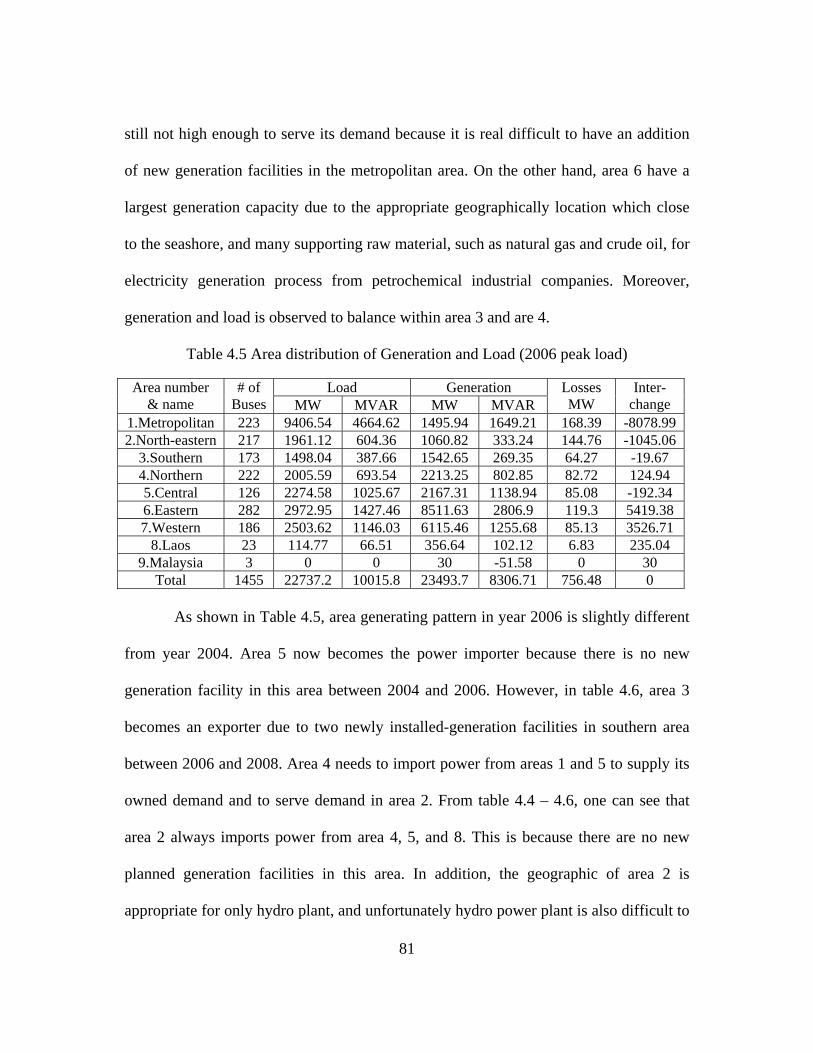
81
still not high enough to serve its demand because it is real difficult to have an addition
of new generation facilities in the metropolitan area. On the other hand, area 6 have a
largest generation capacity due to the appropriate geographically location which close
to the seashore, and many supporting raw material, such as natural gas and crude oil, for
electricity generation process from petrochemical industrial companies. Moreover,
generation and load is observed to balance within area 3 and are 4.
Table 4.5 Area distribution of Generation and Load (2006 peak load)
Load Generation Area number & name
# of Buses MW MVAR MW MVAR
Losses MW
Inter-change
1.Metropolitan 223 9406.54 4664.62 1495.94 1649.21 168.39 -8078.99 2.North-eastern 217 1961.12 604.36 1060.82 333.24 144.76 -1045.06
3.Southern 173 1498.04 387.66 1542.65 269.35 64.27 -19.67 4.Northern 222 2005.59 693.54 2213.25 802.85 82.72 124.94 5.Central 126 2274.58 1025.67 2167.31 1138.94 85.08 -192.34 6.Eastern 282 2972.95 1427.46 8511.63 2806.9 119.3 5419.38 7.Western 186 2503.62 1146.03 6115.46 1255.68 85.13 3526.71
8.Laos 23 114.77 66.51 356.64 102.12 6.83 235.04 9.Malaysia 3 0 0 30 -51.58 0 30
Total 1455 22737.2 10015.8 23493.7 8306.71 756.48 0
As shown in Table 4.5, area generating pattern in year 2006 is slightly different
from year 2004. Area 5 now becomes the power importer because there is no new
generation facility in this area between 2004 and 2006. However, in table 4.6, area 3
becomes an exporter due to two newly installed-generation facilities in southern area
between 2006 and 2008. Area 4 needs to import power from areas 1 and 5 to supply its
owned demand and to serve demand in area 2. From table 4.4 – 4.6, one can see that
area 2 always imports power from area 4, 5, and 8. This is because there are no new
planned generation facilities in this area. In addition, the geographic of area 2 is
appropriate for only hydro plant, and unfortunately hydro power plant is also difficult to

82
implement in system due to the conservative reason. Therefore, there is a high
possibility for the tie lines between area 2 and area 4 to experience with the congestion
problem in the near future. It should be a good indicator for those distributed generators,
or other novel sources of electricity generation from renewable energy to get promoting
in area 2 to alleviate the possible transmission congestion problem.
Table 4.6 Area distribution of Generation and Load (2008 peak load)
Load Generation Area number & name
# of Buses MW MVAR MW MVAR
Losses MW
Inter-change
1.Metropolitan 223 10789.5 5358.19 2879.85 3229.75 133.56 -8043.19 2.North-eastern 217 2244.21 691.6 1103.17 1220.64 270.01 -1411.06
3.Southern 173 1716.97 444.96 2073.23 1133.38 117.87 238.39 4.Northern 222 2295.11 793.65 2391.81 1613.25 134.03 -37.33 5.Central 126 2602.92 1173.72 2294.9 2066.85 138.11 -446.13 6.Eastern 282 3402.11 1633.52 9415.01 3428.61 179.04 5833.85 7.Western 186 2865.03 1311.46 6582.48 1744.16 120.86 3596.59
8.Laos 23 131.34 76.11 381.88 381.72 11.67 238.86 9.Malaysia 3 0 0 30 -54.84 0 30
Total 1455 26047.1 11483.2 27152.3 14763.5 1105.15 0
4.4.3 Area interchange during normal condition
In this section, detail of area interchange between 9 studied areas are
summarized and presented in tables 4.7 – 4.9.
Table 4.7 Area interchange under normal condition (2004 peak load)
Actual tie lines flow (MW) Area To
From Area1 Area2 Area3 Area4 Area5 Area6 Area7 Area8 Area9
Area1 89.5 -876 -3302 -2412 Area2 -483.1 71.1 -252.6 Area3 -92.1 -30 Area4 -89.5 483.1 247.8 Area5 876 -71.1 247.8 -355.2 -405.3 Area6 3302 355.2 Area7 2412 92.1 405.3 Area8 252.6 Area9 30
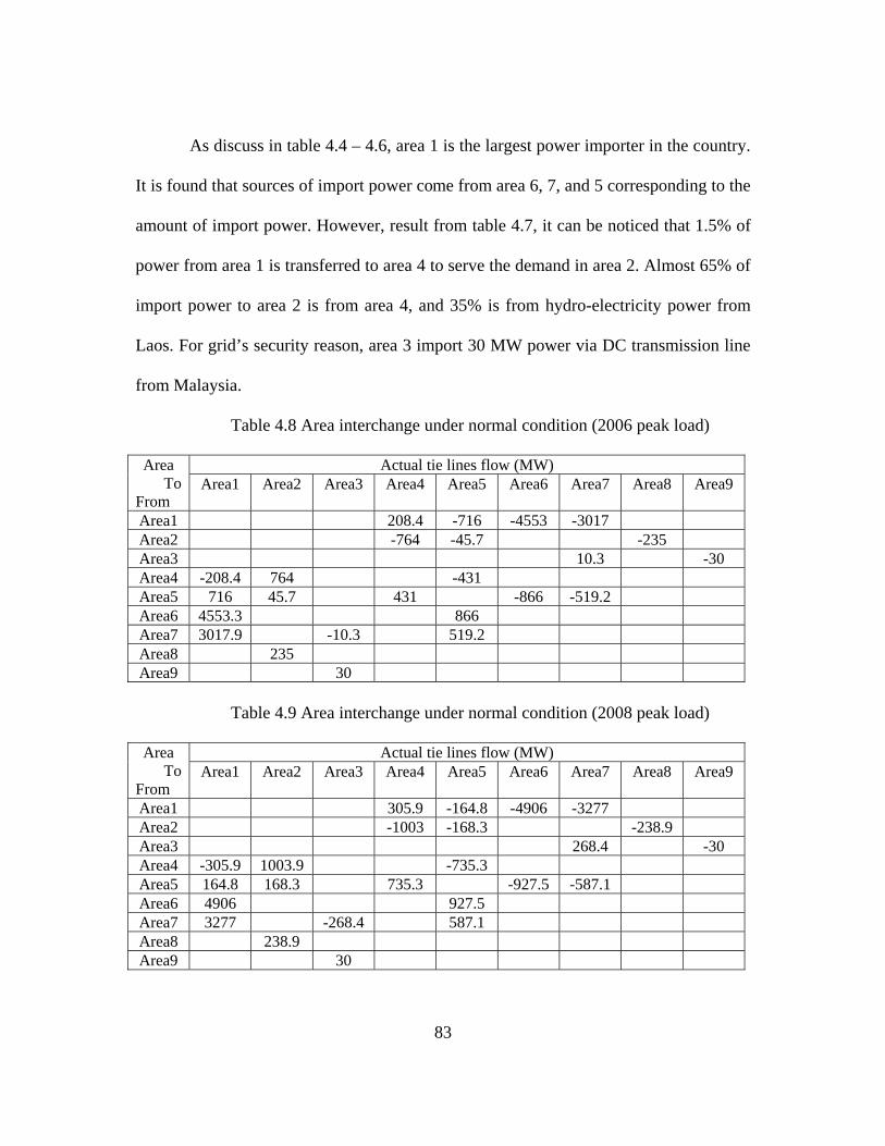
83
As discuss in table 4.4 – 4.6, area 1 is the largest power importer in the country.
It is found that sources of import power come from area 6, 7, and 5 corresponding to the
amount of import power. However, result from table 4.7, it can be noticed that 1.5% of
power from area 1 is transferred to area 4 to serve the demand in area 2. Almost 65% of
import power to area 2 is from area 4, and 35% is from hydro-electricity power from
Laos. For grid’s security reason, area 3 import 30 MW power via DC transmission line
from Malaysia.
Table 4.8 Area interchange under normal condition (2006 peak load)
Actual tie lines flow (MW) Area To
From Area1 Area2 Area3 Area4 Area5 Area6 Area7 Area8 Area9
Area1 208.4 -716 -4553 -3017 Area2 -764 -45.7 -235 Area3 10.3 -30 Area4 -208.4 764 -431 Area5 716 45.7 431 -866 -519.2 Area6 4553.3 866 Area7 3017.9 -10.3 519.2 Area8 235 Area9 30
Table 4.9 Area interchange under normal condition (2008 peak load)
Actual tie lines flow (MW) Area To
From Area1 Area2 Area3 Area4 Area5 Area6 Area7 Area8 Area9
Area1 305.9 -164.8 -4906 -3277 Area2 -1003 -168.3 -238.9 Area3 268.4 -30 Area4 -305.9 1003.9 -735.3 Area5 164.8 168.3 735.3 -927.5 -587.1 Area6 4906 927.5 Area7 3277 -268.4 587.1 Area8 238.9 Area9 30

84
The trend of power flow pattern in year 2006 – 2008 remains almost the same as
of year 2004. Therefore, in the long term, there is a high possibility for an inter-area tie
line to have a congestion problem, especially tie lines between area 1 and 6, and tie
lines between area 1 and 7. It is recommended to keep monitoring those lines closely to
prevent any incident situations.
4.4.4 Major lines flow during normal condition
Since EGAT manages all its owned transmission lines by transferring bulk
power among their operating-regions via 500 kV and 230 kV transmission lines
however, study result shows that most of 500 kV lines are currently use only 30 percent
of their limit. Therefore, these 500 kV line level have a less chances to face with
congestion problem compare to 230 kV lines. As a result, major lines flow result
discussing in table 4.10 – 4.12 will focus on major 230 kV lines.
Result from 2004 base case shows that there is no overloading on the
transmission lines. Major tie lines that transfer power from area 5, 6, and 7 to area 1 are
still operated approximately at 66 percent of their ratings. However, in 2006, the
loadings of nine 230 kV lines reach 80 percent of their limit. As shown in table 4.11,
two of them are using exceed 100 percent of their limit. Therefore, they have already
experienced with an overloading situations. The overloading situations become worst
when system experience with contingency condition as shown in table 4.14.

85
Table 4.10 Major lines flow during 2004 normal condition (above 230 kV)
Lines Percent use of line limit (%) (under normal condition)
From bus To bus Year no. kV no. kV
Circuit
Line limit
(MVA)2004 2006 2008 2010
6802 6802 6801 6801 6802 6802 1804 1804 2801 2801 6802 5804 5804 6804 6804 1807 6891 1809 1809 1811 7801 7801 7801 7801 1810
234.8 234.8 231.8 231.8 234.8 234.8 229.4 229.4 228.7 228.7 234.8 229.9 229.9 235.1 235.1 228.9 233.4 230.4 230.4 229.8 228.6 228.6 228.6 228.6 234
6891 6891 6802 6802 6806 6806 6801 6801 2807 2807 6804 5806 5806 6807 6807 7816 18111 1835 1835 6891 7804 7804 7804 7804 6891
233.4 233.4 234.8 234.8 235.5 235.5 231.8 231.8 230 230
235.1 233.4 233.4 235.1 235.1 225
229.8 229.4 229.4 233.4 236.9 236.9 236.9 236.9 233.4
2 1 1 2 1 2 1 2 1 2 1 2 1 2 1 1 2 2 1 1 1 2 3 4 1
429.4 429.4 429.4 429.4 429.4 429.4 858.9 858.9 429.4 429.4 429.4 858.9 858.9 858.9 858.9 858.9 858.9
1717.7 1717.7 858.9 429.4 429.4 429.4 429.4 858.9
81.4 81.4 80 80
72.7 72.7 66 66
61.5 61.5 61
53.3 53.3 52.8 52.8 50.6 49.6 49.6 49.6 49.6 49.2 49.2 48.8 48.8 48
- - -
Other two tie lines that become more important in year 2006 are tie lines that
link between area 1 to area 5, and area 2 to area 4. This circumstance happen because
area 4 will need to import power from area 1 via transmission line in area 5, then export
the excess power to area 2. This situation becomes clearer in the year 2008 of which
lines usage reach to 90 percent of their limit shown in table 4.12.

86
Table 4.11 Major lines flow during 2006 normal condition (above 230 kV)
Lines Percent use of line limit (%) (under normal condition)
From bus To bus Year no. kV no. kV
Circuit
Line limit
(MVA)2004 2006 2008 2010
6801 6801 6802 6802 6802 6802 6802 1804 1804 2801 2801 5804 5804 1808 1808 1811 6891 1807 3802 3802 2802 2802 1810 1809 1809 1803 1803 6808 6808 1803 1803 3803 3803 6806 6806
231.8 231.8 234.5 234.5 234.5 234.5 234.5 227.9 227.9 223.6 223.6 228.4 228.4 230.3 230.3 226.8 233.4 226.2 236 236
230.9 230.9 231.1 227.7 227.7 225.2 225.2 230.5 230.5 225.2 225.2 237.5 237.5 235.4 235.4
6802 6802 6806 6806 6891 6891 6804 6801 6801 2807 2807 5806 5806 5802 5802 6891 18111 7816 3803 3803 4804 4804 6891 1835 1835 18111 18111 6823 6823 1811 1811 3804 3804 6824 6824
234.5 234.5 235.4 235.4 233.4 233.4 235.1 231.8 231.8 230 230
233.5 233.5 229.8 229.8 233.4 226.8 221.9 237.5 237.5 240.5 240.5 233.4 226.2 226.2 226.8 226.8 234.4 234.4 226.8 226.8 232.7 232.7 235.6 235.6
2 1 1 2 1 2 1 2 1 1 2 1 2 1 2 1 2 1 1 2 1 2 1 1 2 4 3 1 2 2 1 1 2 1 2
429.4 429.4 429.4 429.4 429.4 429.4 429.4 858.9 858.9 429.4 429.4 858.9 858.9 429.4 429.4 858.9 858.9 858.9 429.4 429.4 429.4 429.4 858.9
1717.7 1717.7 858.9 858.9 429.4 429.4 858.9 858.9 429.4 429.4 858.9 858.9
- 102.5 102.5 96.7 96.7 95.6 95.6 81.2 81.1 81.1 71.8 71.8 65.3 65.3 63.7 63.7 62.4 62.4 59.9 59.6 59.6 57.7 57.7 57 57 57
56.9 56.9 56.7 56.7 56.3 56.3 54.6 54.6 54.2 54.2
- -
Showing in year 2008, at least four major 230 kV lines in area 6 will experience
congestion situation. Moreover, power flow for those two tie lines between areas 1 to 5

87
and tie line between areas 2 to 4 become more stress as seen from percent of lines
loading has been increased from 60% in year 2006 to 90% in year 2008.
Main observation from load growth study is that , if monitoring at the same
transmission lines, the average load growth is approximately 14 percent for every two
years (7 percent a year according to MER), while the increasing in line loading is about
10 percent every two years. Therefore, there is a high possibility, for Thailand system,
to have at least ten 230 kV transmission lines facing the congestion problem within the
next few years. The lines flow study under system normal operation presents that, major
transmission lines in area 6 and those inter-area tie lines link with area 1 have a high
possibility, in the near future, to confront with congestion problem. Although all of
them found not to be a severe congestion case at the present time, yet the conditions
become more serious if the system happens to experience with any single contingency,
worse contingencies, or unexpected severe fault.

88
Table 4.12 Major lines flow during 2008 normal condition (above 230 kV)
Lines Percent use of line limit (%) (under normal condition)
From bus To bus Year no. kV no. kV
Circuit
Line limit
(MVA)2004 2006 2008 2010
6801 6801 6802 6802 6802 6802 2801 2801 1808 1808 5804 5804 1804 1804 6802 2802 2802 3802 3802 1811 6891 1810 1803 1803 1807 1803 1803 5802 5802 1805 6808 6808 5801 5801 1805 1805 3808 3808 6806
237.7 237.7 234.8 234.8 234.8 234.8 208.7 208.7 232.7 232.7 230 230
234.1 234.1 234.8 214.1 214.1 228.6 228.6 230.4 237.4 233.9 228.2 228.2 231.7 228.2 228.2 222.7 222.7 242.3 235.8 235.8 224.3 224.3 242.3 242.3 222.3 222.3 235.2
6802 6802 6806 6806 6891 6891 2807 2807 5802 5802 5806 5806 6801 6801 6804 4804 4804 3803 3803 6891 18111 6891 18111 18111 7816 1811 1811 5805 5805 1806 6823 6823 5804 5804 1806 1806 3811 3811 6824
234.8 234.8 235.2 235.2 237.4 237.4 228.5 228.5 222.7 222.7 239.4 239.4 237.7 237.7 235.1 231.5 231.5 237.5 237.5 237.4 230.4 237.4 230.4 230.4 227.2 230.4 230.4 218.1 218.1 234.2 239.8 239.8 230 230
234.2 234.2 227 227
235.5
1 2 2 1 1 2 1 2 1 2 1 2 1 2 1 2 1 2 1 1 2 1 4 3 1 2 1 2 1 1 1 2 2 1 3 2 2 1 2
429.4 429.4 429.4 429.4 429.4 429.4 429.4 429.4 429.4 429.4 858.9 858.9 858.9 858.9 429.4 429.4 429.4 429.4 429.4 858.9 858.9 858.9 858.9 858.9 858.9 858.9 858.9 429.4 429.4 858.9 429.4 429.4 429.4 429.4 858.9 858.9 429.4 429.4 858.9
- - 108.9 108.9 100.3 100.3 96.7 96.7 91.3 91.3 90.9 90.9 86.3 86.3 85 85
80.1 76.2 76.2 72 72
69.5 69.5 66.8 65.7 65.7 65.1 65 65
64.3 64.3 63
61.2 61.2 60.4 60.4 59.7 59.7 59.5 59.5 58.8
-
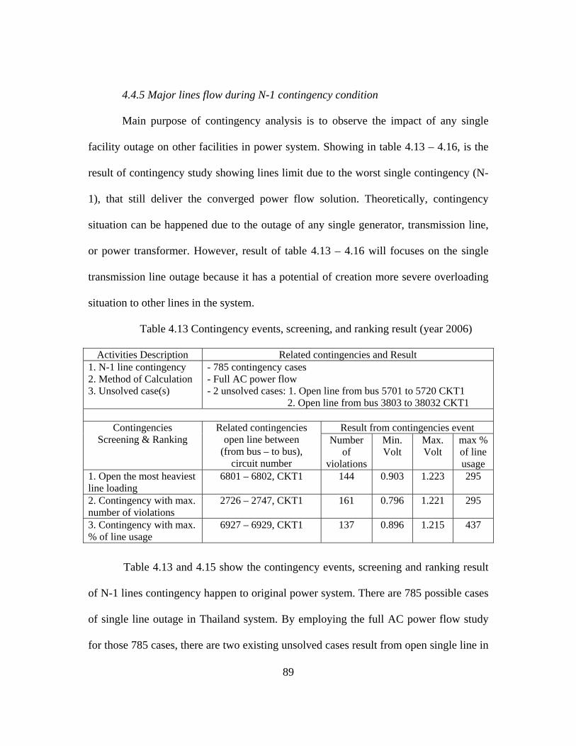
89
4.4.5 Major lines flow during N-1 contingency condition
Main purpose of contingency analysis is to observe the impact of any single
facility outage on other facilities in power system. Showing in table 4.13 – 4.16, is the
result of contingency study showing lines limit due to the worst single contingency (N-
1), that still deliver the converged power flow solution. Theoretically, contingency
situation can be happened due to the outage of any single generator, transmission line,
or power transformer. However, result of table 4.13 – 4.16 will focuses on the single
transmission line outage because it has a potential of creation more severe overloading
situation to other lines in the system.
Table 4.13 Contingency events, screening, and ranking result (year 2006)
Activities Description Related contingencies and Result 1. N-1 line contingency 2. Method of Calculation 3. Unsolved case(s)
- 785 contingency cases - Full AC power flow - 2 unsolved cases: 1. Open line from bus 5701 to 5720 CKT1 2. Open line from bus 3803 to 38032 CKT1
Result from contingencies event Contingencies
Screening & Ranking Related contingencies
open line between (from bus – to bus),
circuit number
Number of
violations
Min. Volt
Max. Volt
max % of line usage
1. Open the most heaviest line loading
6801 – 6802, CKT1
144 0.903 1.223 295
2. Contingency with max. number of violations
2726 – 2747, CKT1
161 0.796 1.221 295
3. Contingency with max. % of line usage
6927 – 6929, CKT1
137 0.896 1.215 437
Table 4.13 and 4.15 show the contingency events, screening and ranking result
of N-1 lines contingency happen to original power system. There are 785 possible cases
of single line outage in Thailand system. By employing the full AC power flow study
for those 785 cases, there are two existing unsolved cases result from open single line in

90
area 5 and area 3 respectively. Due to a large number of contingency cases, techniques
of contingency screening and ranking need to be deployed in order to reduce the
number of studied-cases. Thus, in this dissertation, three contingency scenarios are
focused i.e. 1) open single line with the largest line loading, 2) open one line with
generating the maximum number of violations, and 3) open a line with causing other
lines to confront with the most severe overloading. The result of contingencies
screening in table 4.13 and 4.14 shows that opening a single line in area 6 appears to
create more severe violation cases of lines overloading, and to increase the loading level
of other lines in the same area.
The similar trend of contingency events is found in table 4.15 and 4.16 for the
year 2008. There are 785 cases of N-1 line contingencies to be considered. After
performing a full ACPF for all contingency cases, there are 8 cases of diverged power
flow solutions. This situation implies the more complexity of power system pattern in
year 2008 compare to year 2006, and some delicate quantities need to be addressed such
as: reactive power supply and voltage issue, power system protection issues, and power
quality issue.

91
Table 4.14 Major lines power flow during N-1 contingency (year 2006)
Lines Percent use of line limit (%) (under contingency condition)
From bus To bus Year no. kV no. kV
Circuit
Line limit
(MVA)2004 2006 2008 2010
6801 6802 6802 6802 6802 2801 2801 1804 1804 6802 6891 1811 5804 5804 1808 1808 1810 1807 3802 3802 2802 2802 6808 6808 1803 1803 1809 1809 1803 1803 3803 3803 6806 6806 1804 1804 7801
233.4 234.6 234.6 234.6 234.6 224.4 224.4 229.9 229.9 234.6 235.4 228.7 229.9 229.9 231.5 231.5 232.6 227.9 236.1 236.1 232.4 232.4 232 232
227.2 227.2 229.2 229.2 227.2 227.2 237.5 237.5 235.7 235.7 229.9 229.9 226.4
6802 6891 6891 6806 6806 2807 2807 6801 6801 6804 18111 6891 5806 5806 5802 5802 6891 7816 3803 3803 4804 4804 6823 6823 18111 18111 1835 1835 1811 1811 3804 3804 6824 6824 1813 1813 7804
234.6 235.4 235.4 235.7 235.7 230 230
233.4 233.4 235.4 228.7 235.4 234.7 234.7 230.9 230.9 235.4 223.7 237.5 237.5 241.6 241.6 236 236
228.7 228.7 227.8 227.8 228.7 228.7 232.8 232.8 235.9 235.9 230.8 230.8 236.9
2 1 2 2 1 2 1 2 1 1 2 1 1 2 2 1 1 1 2 1 1 2 1 2 4 3 2 1 2 1 2 1 1 2 2 1 1
429.4 429.4 429.4 429.4 429.4 429.4 429.4 858.9 858.9 429.4 858.9 858.9 858.9 858.9 429.4 429.4 858.9 858.9 429.4 429.4 429.4 429.4 429.4 429.4 858.9 858.9
1717.7 1717.7 858.9 858.9 429.4 429.4 858.9 858.9 858.9 858.9 429.4
143.5 112.8 112.8 91.3 91.3 71.1 71.1 71 71
69.8 66.9 66.9 64.4 64.4 62.7 62.7 62.1 59.6 59.5 59.5 57.1 57.1 56.6 56.6 56.5 56.5 56.1 56.1 55.9 55.9 54.3 54.3 54 54
51.8 51.8 49.1

92
Table 4.15 Contingency events, screening, and ranking result (year 2008)
Activities Description Related contingencies and Result 1. N-1 line contingency 2. Method of Calculation 3. Unsolved case(s)
- 785 contingencies - Full AC power flow - 8 unsolved cases: 1. Open line from bus 2726 to 2747 CKT1 2. Open line from bus 7706 to 7707 CKT1 3. Open line from bus 4741 to 4744 CKT1 4. Open line from bus 2705 to 2707 CKT1 5. Open line from bus 4808 to 4812 CKT1 6. Open line from bus 4808 to 4812 CKT2 7. Open line from bus 5701 to 5720 CKT1 8. Open line from bus 7706 to 7708 CKT1
Result from contingencies event Contingencies
Screening & Ranking Related contingencies
open line between (from bus – to bus),
circuit number
Number of
violations
Min. Volt
Max. Volt
max % of line usage
1. Open most heaviest line loading
6801 – 6802, CKT1
600 0.502 1.361 865.8
2. Contingency with max. number of violations
6908 – 6909, CKT1
602 0.463 1.362 865.2
3. Contingency with max. % of line usage
2726 – 2746, CKT2
589 0.440 1.361 872.3
Due to the higher in electricity demand, and uncertainty of newly installed
generation locations, result of N-1 contingencies cases from table 4.15 – 4.16 of year
2008 is more severe than those cases in year 2006. Comparing result of 4.13 and 4.15, it
is found that 2008 contingency cases potentially create up to 600 violations while only
150 violations were observed in year 2006. Besides, two major observations obtained
from these contingency studies are 1) single transmission facilities outage in area 6
tends to create the overloading problem to system due to inadequate transmission lines
to transfer power to load center and 2) single transmission outage in area 2 is likely to
create low voltage problem due to insufficient generation facilities within this area. This

93
outcome can be verified from table 4.9 where 1000 MW of transfers from area 4 to area
2.
Table 4.16 Major lines power flow during N-1 contingency (year 2008)
Lines Percent use of line limit (%) (under contingency condition)
From bus To bus Year no. kV no. kV
Circuit
Line limit
(MVA)2004 2006 2008 2010
6801 6802 6802 6802 6802 2801 2801 1808 1808 5804 5804 2802 2802 1811 6891 1804 1804 1810 3802 3802 6802 1803 1803 1807 1803 1803 5802 5802 1805 1804 1804 6808 6808 5801 5801 1805 1805
239.7 234.7 234.7 234.7 234.7 209.3 209.3 233.6 233.6 231.4 231.4 214.4 214.4 231.2 237.2 235.5 235.5 234.5 229.2 229.2 234.7 229.1 229.1 233.1 229.1 229.1 223.8 223.8 243.7 235.5 235.5 237.7 237.7 226.2 226.2 243.7 243.7
6802 6891 6891 6806 6806 2807 2807 5802 5802 5806 5806 4804 4804 6891 18111 6801 6801 6891 3803 3803 6804 18111 18111 7816 1811 1811 5805 5805 1806 1811 18111 6823 6823 5804 5804 1806 1806
234.7 237.2 237.2 235.2 235.2 229.2 229.2 223.8 223.8 240.5 240.5 232.4 232.4 237.2 231.2 239.7 239.7 237.2 237.5 237.5 234.8 231.2 231.2 228.7 231.2 231.2 219.2 219.2 235.6 231.2 231.2 241.7 241.7 231.4 231.4 235.6 235.6
2 1 2 2 1 2 1 1 2 1 2 1 2 1 2 2 1 1 2 1 1 4 3 1 2 1 2 1 1 1 2 1 2 2 1 3 2
429.4 429.4 429.4 429.4 429.4 429.4 429.4 429.4 429.4 858.9 858.9 429.4 429.4 858.9 858.9 858.9 858.9 858.9 429.4 429.4 429.4 858.9 858.9 858.9 858.9 858.9 429.4 429.4 858.9 429.4 429.4 429.4 429.4 429.4 429.4 858.9 858.9
157.2 113.8 113.8 95.4 95.4 91.6 91.6 90.6 90.6 85.7 85.7 76.4 76.4 75.2 75.2 75.2 75.2 73.7 71.8 71.8 68.8 65.6 65.6 65
64.9 64.9 64.2 64.2 62.9 62.1 61.9 61.3 61.3 59.7 59.7 59.7 59.7

94
4.5 Chapter summary
The study of steady state power flow in Thailand system, according to EPPO’s
load forecasting result and Thailand power development plan (PDP03-04) indicate that,
under the traditional operation, the country could experience with transmission
congestion problem in year 2006. The situations become worse if system will
experience with any contingency conditions. All result in section 4.4 designates the
power balance between generation and load in each pre-defined study areas. Area 1,
metropolitan and its vicinity is the biggest power importer area, while area 2 located in
the north-east part of the country is showing consistent growing in power importer since
there is no new generation facilities projects to be online within this area. Area 6 and
area 7 have a similar ratio of generation and demand within their areas and considered
to be a significant power supplier for other areas in the country. Moreover, due to a high
transfer between area 1 and its supplier areas (area 5, 6, and 7), it is most likely for
interfaces between area 1 and its supplier can be good candidacies for CSCs selection.
Finally, all study result in chapter 4 including: converged power flow cases, area
distribution of generations and loads, and tie lines flow study, will be used as primary
input for the transmission congestion management study in chapter 5.

95
CHAPTER 5
PROPOSED TCM MODELS DURING TRANSITION PERIOD
5.1 Introduction and relevant limitations
Changing from the traditional vertically integrated system to a deregulated
environment creates numerous challenging tasks to system operators (SOs). Significant
number of electricity transactions both in day ahead and real time market lead to the
difficulty in power flow prediction. Therefore, the concept of congestion management is
emerged. Theoretically, the idea of TCM is to alleviate the amount of power flow in the
congested transmission lines by changing the flow pattern. This process of re-dispatch
can be done by modifying generation, or modifying load, or both without compromising
the system security and service quality [15].
As a developing country with the gross income disparity among the population,
social equity policy should and would be pursued by the government. In this respect,
equitable access to electricity irrespective of geographical location is desirable and
some form of subsidy for lower income groups should still be implemented [61]. In
addition, the current structure of OASIS, computer information technology including
the high speed internet services is still under the developing stage. These factors could
become vital limitations for congestion management processes proposed in this chapter.

96
Main ideas of this chapter are to discuss and propose the implementation
procedures of two CM schemes which are Zonal Congestion Management (ZCM) and
Nodal Congestion Management (NCM). Chapter starts with the proposed modified
ERCOT-model regarding to RTO/ISO’s core businesses. Then, required-data and
implementation procedures of ZCM and NCM will be proposed, followed by generation
cost comparison of three dispatching scenarios which results from different CM
schemes. These three scenarios are composed of 1) EGAT stays with traditional
operation mode, 2) EGAT moves to deregulated environment with NCM, and 3) EGAT
utilizes ZCM for managing transmission congestion.
5.2 Proposed modified-ERCOT model for RTO/ISO core-functions
The deregulated power market is a brand-new concept to MPs in Thailand.
Without well defined rules to control and monitor all MPs, it can lead to another
disaster similar to California crisis in 2000. Hence, it is a root important to establish a
structure of core-functions responsible by the regulatory body. Fig. 5.1 is the typical
core-functions of Regional Transmission Organization/Independent System Operator
(RTO/ISO). According to this chart, the primary mission of RTO/ISO is to ensure
security of system operation. According to the operation timeframe of ISO, the bilateral
contract market and load forecasting would be main charges for ISO in the pre-Day
ahead market. Day Ahead (DA) energy market, DA ancillary services, and DA
reliability unit commitment are three main tasks in the Day Ahead Market. The
balancing energy market would be implemented on real time (RT) market with the

ancillary services deployment. Finally, settlement process (SA) will be handled after the
real time market.
Figure 5.1 RTO/ISO core-functions [modified 41]
For all MPs, financial incentive is the most important factor for them to justify
whether to join the market at the particular time. Typically, there are at least 4 main cost
components for each MP. As shown in Fig. 5.2, the basement of this cost component is
bilateral contract cost between two parties. DA cost component will be provided to all
MPs after DA clearing process. Since the real time cost can vary significantly, MPs can
control their risk in real time pricing by using other options such as FTR or TCR. The
last component is from the uninstructed resource charge. Depending on the different
between actual and scheduling power in which they commit to provide and/or consume,
this element can cost or award MPs.
97

Figure 5.2 Typical cost components for all MPs
5.3 Discussion on typical Market Structures
5.3.1 Day-Ahead Market
The primary objective of DA market is to create a financial binding schedule for
both energy and ancillary service. According to ERCOT 95% confidence level, ERCOT
has obtained energy market as close to 95% after settled DA transactions. In this
manner, ERCOT can operate system with a high level of security confident. At the
mean time, for MPs, knowing 95% of scheduling transaction would provide less risk in
their financial obligation. Typically, there are two types of DA market i.e., DA with
transmission constraints and without transmission constraints. The former is more
complicate due to ISO needs to know all outage scheduling and run all contingency
cases. The latter is less complicate because ISO will clear market base on network
topology as well as supply and demand bids.
For the DA market in the ISO/RTO, Security Constraints Unit Commitment
(SCUC) will be used as a main tool to assure the adequacy of generation resources for
the next-day in order to have a good solution of economic dispatch (ED) in RT market.
98

Then, Security Constraint Economic Dispatch (SCED) is deployed to obtain the
converged power flow case and a good dispatching pattern. During the DA price
calculation, the process can be different depending on whether ZCM or NCM be
utilized in the system. In addition, DA price components in the settlement bill can
include energy price, transmission price, load zone price, HUB price, and Point to Point
price. Figure 5.3 shows the typical structure of DA market mentioned above.
Figure 5.3 Typical Day Ahead market structure
To apply in the Thailand system, it is recommend that DA market structure with
considering transmission constraints be used because it reflects more realistic situations
and ISO can have better confidence in operating and controlling system.
5.3.2 Real Time Energy Balancing Market
In order to maintain the system frequency in real time operation, ISO needs to
keep balancing between generation resources and demand for the entire the system.
Therefore, RT market can be considered as the most important market because it
provides the last resource of energy transaction to generations and consumers. It is clear 99

from figure 5.3 and 5.4 that typical structure of RT and DA markets are similar. In the
RT operation, real time data from SCADA system would be the basic data for the RT
market clearing price process. ISO then, deploys SCED subject to unit ramp rate,
energy reserve, and energy balance constraints to obtain a feasible, and fast enough
dispatching instruction. The SCED solution will be used in the process of RT price
calculation. Similar to DA market, RT pricing can be based on either ZCM or NCM
depend on the system congestion management structure. Throughout the process of
SCED, ISO will use bid curve from MPs instead of heat rate curve as used in the
traditional ED. Since it requires fast converged solution, all calculation will base only
on real power flow concept. Figure 5.4 illustrates the typical configuration of RT
market.
Figure 5.4 Typical Real Time Balancing Energy market structure
100

101
5.4 Basic Assumptions
5.4.1 Power Flow Study
As stated in chapter 4, power flow study is to determine the 1) steady-state
flows through lines and transformers and 2) bus voltages throughout the system under
specific conditions. These values are examined to assure that no line flow is above its
normal limits (95 percent of the nominal limit) and no bus voltage is outside its normal
operating range (0.95 pu. to 1.05 pu.). It should be noted that the summer peak load was
selected as the power flow base case for the entire dissertation since it has higher
possibility to cause transmission congestion problem.
5.4.2 Optimal Power Flow Study
Theoretically, the main purpose of Optimal Power Flow (OPF) is to optimize
the objective function which is total operating cost in this dissertation. This objective
function is accomplished by changing different system control variables while meeting
power balance constraints and enforcing operating limits. OPF program will adjust the
generation level automatically to find the least-cost or least-price generation dispatch
while observing the transmission limits. Thus, while power flow simulates performance
of system under specified conditions, the OPF optimizes system performance to meet
specified objective function.
In general, solving optimization problems involve two types of constraints
which are equality and inequality constraints. Equality constraints always have to be
enforced such as real and reactive power balance equations and area MW interchanges
constraints. Inequality constraints, on the other hand, may or may not be binding. For

example, a line MVA flow or generator real power output may or may not be at its
maximum limit. Since OPF is solved by iterating between a power flow (PF) solution
and linear programming (LP) solution, therefore it is possible for some constraints to be
enforced during PF solution, and some constraints are enforced during LP solution.
In order to solve a nonlinear and constraints-optimization problem, OPF
requires the cost curve of each generator to perform an economically optimal power
flow. In this dissertation, linear piecewise cost curves are the input data of the OPF
study processes. In addition, to guarantee a converged and fast power flow solution
during the real time operating condition, a DC power flow (DCPF) model was utilized.
Therefore, for comparison purpose, a DCPF model will be used for the traditional
operation pattern. On the other hand, DCOPF model will be applied for both ZCM and
NCM. Following objective function and constraints will be taken into consideration
when performing DCOPF.
5.4.2.1 OPF objective function
A main objective function for this dissertation is to maximize social welfare. In
other words, it is to minimize total generation cost from all online generating units. This
objective function can be expressed as,
(5.1) ∑=
=NG
iii PCJ
1)(min
Where, J: total system generation cost
Ci(Pi): units’ generating cost
NG: set of all generating units including slack bus.
102

5.4.2.2 Network equations
Since the study of generation cost comparison in this dissertation is based on
DC model, real power generation equation at each node obtained from basic Kirchoff’s
Laws will be included in the OPF problem. These real power balance equations can be
treated as equality constraints and can be expressed as,
( )∑ −+=−j
ijjijijiii YVVPDP δδθ ,, cos slackiNi ∉=∀ :,...,1 (5.2)
Where, V: the bus voltage
δ : the angle associated with V
: the element of bus admittance matrix jiY ,
θ : the angle associated with jiY ,
Pi: real power generation at bus i
PDi: real power demand at bus i
N: the number of buses in system
5.4.2.3 Generation limits
The generation real power limit is considered to be an inequality constraint
which may or may not be binding, and can be presented as,
maxminiii PPP ≤≤ NGi∈∀ (5.3)
Where, Pmin and Pmax: the lower and upper limits on real power generation
103

5.4.2.4 Transmission lines limits
In this study, transmission line limit is based on rate A (normal operating) which
is usually determined by the thermal limit capacity of lines. This limit is considered as
an inequality constraints and can be expressed as,
Maxjiji PP ,, ≤ 0, ≠∀ jiY (5.4)
Where, Pi,j : the power flow over a line i-j
PMaxi,j : the maximum limit on power flow over the line.
5.5 Implementation of Zonal Congestion Management in Thailand System
Main purposes of ZCM are to 1) predict potential congestion on those
Commercial Significant Constraints (CSCs), 2) perform necessary adjustment in the
day-ahead market and notify the market participants, and 3) determine if replacement
resources should be purchased in a congestion zone [67]. When implement in Thailand
system, ISO will have the responsibilities to manage transmission congestion, and will
categorize the cost of congestion as either Zonal Congestion Management (ZCM), or
Local Congestion Management (LCM). ZCM costs are those costs that ISO used to
manage congestion on CSCs.
5.5.1 Required Data
The most important data required before performing CMZs determination is the
power flow base case data. The responsible-committee or working group needs to
provide the upcoming year’s summer peak power flow base case (planning data). This
power flow base case should contain following important information:
104

105
a) The planning year’s peak summer load.
b) The planning year’s scheduled generating unit additions, retirement, and
ratings.
c) The planning year’s scheduled transmission facility additions, retirement, and
ratings.
d) The list of actual contingency events over the past twelve months, with
associated cost impact on the system. This data, if provided, will be used as a
pilot data for CSCs determination processes.
It should be noted that if there is no significant system changes for the upcoming
year and there is no significant cost impact from contingencies, the upcoming year’s
CMZs will remain the same. Otherwise, it is ISO’s responsibility to determine the
potential CSCs and re-clustering new CMZs to be used in the upcoming year.
5.5.2 CM Zones Determination based on ERCOT’s Method
In this section, the proposed steps of defining CMZs within Thailand system
will be similar to processes in ERCOT [42, 67-68]. CMZs are to be determined by
subjectively evaluating results of cluster analysis. The input data for the cluster analysis
is a set of Generation Shift Factors (GSFs) which obtains from a DCPF analysis. The
shift factors are associated with each bus in the system and collectively determine the
line flow on the CSC [42]. Following are four main steps in CMZs determination
proposed in this dissertation:

106
5.5.2.1 Determination of CSCs
Since Thailand is at its initial stage moving toward deregulation, it should take a
more conservative approach in determining CSCs. Because CSC determination is a
subjective step, it requires engineering judgment based on the annual technical and
financial analysis. A subcommittee from ISO and EPPO should be a proper starter team
to take the responsibility of this task. New CSCs for the upcoming year, as well as the
electrical network topology, should be defined annually by September 30th to match the
fiscal year of Thailand. The analysis should be based on “Summer Peak Load Flow
Case” and performing steady state power flow, contingency analysis, and dynamic
stability analysis. After the completion of all studies, load flow cases used in
determining CSCs should be posted on the ISO’s website.
Since this is the first time that the zonal congestion management is implemented
in Thailand, it is recommend that a minimum number of congestion zones be
implemented to minimize the complexity in operation and control for SO and simple for
MPs. The selection of CSCs candidacies will be start at year 2006 because there is a
first emergence of transmission congestion problem. The same CSCs candidacies will
be used in the CMZs determination for year 2008 as well.
The simulation results in table 5.1 indicate that the loading of the 500 kV lines
are approximately 20% of their limit, therefore these 500 kV lines are unlikely to have
congestion problem in the near future. According to the results from table 5.1 – 5.5, the
potential candidates for CSCs should be the major high voltage inter-area tie lines
which carry heavy flows. Although there are 9 studied regions for the original system as

107
introduced in Chapter 4, area 8 and 9 are the neighboring countries. Therefore, only 7
domestic regions will be focused in CSCs determination processes. It is found that all 7
areas can generate 12 combination scenarios of tie lines flow as listed in table 5.1 – 5.5.
Table 5.1Inter-area power transfer from area 1 (Year 2006)
Scenarios of Interfaces or CSCs candidacies
From bus
From bus To bus No.
Area kV No. Area kV No.
Circuit
Line limit
(MVA) Actual MW Flow
% use of
MVA 1 1
1 1 1 1 1 1 1 1
230.3 230.3 227.7 227.7 227.7 227.7 500.6 500.6 500.6
1808 1808 1809 1809 1809 1809 1908 1908 1908
5 5 5 5 5 5 5 5 5
229.8 229.8 234.7 234.7 233.5 233.5 503.4 503.4 503.4
5802 5802 58061 58061 5806 5806 5906 5906 5906
1 2 3 4 2 1 1 3 2
429.4 429.4 858.9 858.9 858.9 858.9
3734.1 3734.1 3734.1
273.1 273.1 -389.2 -389
-248.8 -248.8 147.7 120.7 147.7
63.7 63.7 47 47
30.4 30.4 5.4 4.6 4.6
2 1 1 1 1 1 1 1
227.9 227.9 226.8 231.1 498.6 227.7 227.7
1804 1804 1811 1810 6661 1809 1809
6 6 6 6 6 6 6
231.8 231.8 233.4 233.4 501.5 230.5 230.5
6801 6801 6891 6891 6911 6808 6808
2 1 1 1 1 2 1
858.9 858.9 858.9 858.9
2833.6 858.9 858.9
-683.9 -683.9 -521.8 -484
-1085 -282 -282
81.1 81.1 62.4 57
38.8 33.2 33.2
3 1 1 1 1 1 1 1
226.2 227.2 226.4 226.4 500.6 500.6 500.6
1807 1806
25 24
1908 1908 1908
7 7 7 7 7 7 7
221.9 221.9 225.9 225.9 509.2 509.2 509.2
7816 7816 7801 7801 7902 7902 7902
1 1 2 1 3 2 1
858.9 858.9
1717.7 1717.7 3734.1 3734.1 3734.1
444.5 243.9 -506.3 -506.3 -897.9 -897.9 -897.9
59.9 38.2 29.7 29.7 24.8 24.5 24.5
Scenario 1 – 3 in table 5.1 is potentially CSCs candidates between area 1 and
areas 5, 6, and 7. The most likely CSC candidates within table 5.1 are two lines link
between area 1 and area 6 from in scenario no. 2. This CSC candidacy currently reaches
81 percent of its 860 MVA limit. Another possible candidacy is the interface from
scenario no. 1 which is the 230 kV lines between bus 1808 and bus 5802. The loading

108
of this line is 65 percent of its maximum 430 MVA limit. The last possible candidacy is
the interface from scenario no. 3 which is the 230 kV line between bus 1807 and bus
7816 with the current loading at 60 percent of its maximum 860 MVA.
Table 5.2 Inter-area power transfer from area 2 (Year 2006)
Scenarios of Interfaces or CSCs candidacies
From bus
From bus To bus No.
Area kV No. Area kV No.
Circuit
Line limit
(MVA) Actual MW Flow
% use of
MVA 4 2
2 2 2
230.9 230.9 231.4 231.4
2802 2802 2803 2803
4 4 4 4
230.9 230.9 231.4 231.4
4804 4804 4807 4807
1 2 1 2
429.4 429.4 429.4 429.4
-237.6 -237.6 -132.3 -132.3
57.7 57.7 32.1 32.1
5 2 2 2 2
112.7 113.8 230 230
2701 2702 2807 2807
5 5 5 5
117.8 117.8 229.3 229.3
5708 5708 5803 5803
1 1 2 1
117.5 117.5 429.4 429.4
-77.9 -55.5 46.8 46.8
69.2 49.8 11 11
6 2 2 2 2 2 2 2 2 2
116.9 113
237.2 230.6 230.6 117.5 113
114.2 237.9
2723 2736 2811 2808 2808 2740 2736 2733 2810
8 8 8 8 8 8 8 8 8
118 112.6 237.9 230 230
117.6 113.1 113.1 237.9
2888 8736 8000 8004 8004 8705 8734 8734 8000
1 1 1 1 2 1 1 1 1
119.5 57.1
429.4 429.4 429.4 119.5 119.5 119.5 429.4
16.6 2
-77.4 -65 -65
-18.6 -11.2 8.7 -25
33 24.4 18.4 16.4 16.4 15.8 9.9 7.5 6.3
Results of table 5.2 are tie lines link between area 2 and its supply areas.
Majority of import power comes from area 4, therefore, the most likely to be a
candidacy for CSC should be lines between bus 2802 and 4804. The loading of these
230 kV lines are 60 percent of their 430 MVA maximum limit.
It is clear from scenario no. 7 in table 5.3 that the tie line between area 3 and
area 7 still has enough room for transferring power in the near future. Therefore, this
scenario will not create any CSC candidacy in this year.

109
Table 5.3 Inter-area power transfer from area 3 (Year 2006)
Scenarios of Interfaces or CSCs candidacies
From bus
From bus To bus No.
Area kV No. Area kV No.
Circuit
Line limit
(MVA) Actual MW Flow
% use of
MVA 7 3
3 3 3
116.7 116.7 236 236
3701 3701 3802 3802
7 7 7 7
117.4 117.4 243.2 243.2
7721 7721 7829 7829
1 2 2 1
119.5 119.5 429.4 429.4
-22.7 -22.7 27.9 27.9
19.6 19.6 11.2 11.2
Table 5.4 Inter-area power transfer from area 4 (Year 2006)
Scenarios of Interfaces or CSCs candidacies
From bus
From bus To bus No.
Area kV No. Area kV No.
Circuit
Line limit
(MVA) Actual MW Flow
% use of
MVA 8 4 502.7 4441 1 498.6 6661 1 2833.6 -232.4 9.8 9 4
4 4 4 4 4 4 4
240.5 240.5 240.5 240.5 502.7 502.7 237.4 237.4
4804 4804 4804 4804 4441 4441 4803 4803
5 5 5 5 5 5 5 5
227.5 227.5 230.4 230.4 503.4 503.4 229.8 229.8
5805 5805 5801 5801 5906 5906 5802 5802
2 1 2 1 2 1 2 1
858.9 858.9 429.4 429.4
2833.6 2833.6 429.4 429.4
191.5 191.5 -25.6 -25.6
-392.2 -392.2
8.5 8.5
23.8 23.8 14.6 14.6 14.4 14.4 9.8 9.8
Results of table 5.4 and 5.5 show no potential line to be a CSC candidacy. In
summary, from the operation record and power transfer study result shown in table 5.1
– 5.5, the most likely potential interfaces to become CSCs candidacies in Thailand
system can be priority listed as shown in table 5.6

110
Table 5.5 Inter-area power transfer from area 5 (Year 2006)
Scenarios of Interfaces or CSCs candidacies
From bus
From bus To bus No.
Area kV No. Area kV No.
Circuit
Line limit
(MVA) Actual MW Flow
% use of
MVA 10 5
5 503.4 503.4
5906 5906
1 1
498.6 498.6
6661 6661
2 1
2833.6 2833.6
201.4 201.4
9.6 8.6
11 5 503.4 5906 6 501.5 6911 1 2833.6 -866 30.8 12 5 503.4 5906 7 509.2 7902 1 3734 -519.2 14.3
Table 5.6 CSCs candidacies for Year 2006
MVA CSC no. CSC Name Scenario, (circuit)
Between Areas
Loading (MW) Limit %Loading
CSC1 CSC Metro-East 2, (2) 1 and 6 684 860 81 CSC2 CSC Metro-West 3, (1) 1 and 7 444 860 60 CSC3 CSC Metro-Central 1, (2) 1 and 5 273 430 65 CSC4 CSC North-North East 4, (2) 4 and 2 238 430 58
After finishing CSCs determination process in step 1, it is necessary to calculate
generation shift factor and re-cluster the system to create new CMZs if there is any
potential for new lines or interfaces to experience congestion problems in the coming
year.
5.5.2.2 Power Transfer Distribution Factor (PTDF) or Shift Factor Calculation
Unlike the previous step, this step is mathematical processes. The main purpose
of calculating the Power Transfer Distribution Factor (PTDF) or shift factor (SF) is to
determine the impact of transferring one MW from a specific bus to the system
slack/reference bus on the power flow of each pre-defined interfaces (CSCs) from
previous step. Two existing concepts for SFs calculations are explained below [67]:

111
Type 1—defines as effect of 1 MW of transfer from a particular bus to system
slack bus on a specified line or CSC.
Type 2—defines as effect of 1 MW of transfer from a particular bus to a
designated reference bus on a specified line or CSC.
This dissertation adopts the type 1 SF calculation for Thailand system in the
initial stage of classifying CMZs. It should be noted that for Thailand system, the
system slack bus is located in area 6. The SFs are to be calculated for all buses for the
entire system. Since 1 MW will not change the system operation condition significantly,
linear lossless DC model is used for calculating PTDF for proposed CSCs interfaces.
Currently, there are almost 1500 buses in Thailand system. It can generate a
large number of numerical results of shift factors therefore not all of them will be listed
in this dissertation. Table 5.7 shows some of PTDFs impact on four pre-defined CSCs
(table 5.6). The shift factors listed in Table 5.7 are the impact of transferring additional
1 MW from a particular bus to system slack bus (bus 6003 in area 6) on four CSCs. For
example, if 1 MW transfers from bus 7005 to system slack bus, it will increase flow by
0.038 MW, 0.03 MW, and 0.198 MW on CSC1, CSC2, and CSC4 respectively.
However, this 1 MW transfer will, at the same time, reduce the flow on CSC3 by 0.225
MW.

112
Table 5.7 Example of PTDF or SF calculating for each CSC
Power Transfer Distribution Factor (PTDF) or Generation Shift Factor (GSF) on CSCs
Bus No. Bus Name Area No.
CSC1 Metro to
East
CSC2 Metro to
West
CSC3 Metro to Central
CSC4 North east to North
1013 1021 1022 1023 1031 1032 1033
SB-T3 SB-C11 SB-C12 SB-C10 SB-C21 SB-C22 SB-C20
1 1 1 1 1 1 1
-0.113 -0.113 -0.113 -0.113 -0.113 -0.113 -0.113
0.032 0.032 0.032 0.032 0.032 0.032 0.032
-0.333 -0.313 -0.299 -0.299 -0.298 -0.298 -0.29
0.199 0.271 0.321 0.321 0.323 0.323 0.335
2011 2012 2014 2203 2204 2205 2206
LTK-H1 LTK-H2 LTK-H4
SKI-1 SKI-2 NR2-1 NR2-2
2 2 2 2 2 2 2
-0.001 -0.001 -0.001 -0.001 -0.001 -0.001 -0.001
0.031 0.031 0.031 0.031 0.031 0.031 0.031
-0.257 -0.257 -0.257 -0.257 -0.257 -0.257 -0.257
0.386 0.386 0.386 0.387 0.387 0.387 0.387
6001 6002 6801 631 632 633
6104
BPK-T1 BPK-T2 BPK-A KLM-1J KLM-2J KLM-3J
EPEC-CC1
6 6 6 6 6 6 6
0.445 0.445 0.445 0.405 0.405 0.405 0.405
0.032 0.032 0.032 0.032 0.032 0.032 0.031
-0.001 -0.001 -0.001 -0.001 -0.001 -0.001 -0.256
0 0 0 0 0 0
0.389 7005 7006 7011 7007 7804 7723 7720
SNR-H5 TTN-H1 VRK-H1 TTN-H2
SNR RB3-WP
PKK
7 7 7 7 7 7 7
0.038 0.037 0.038 0.037 0.038 0.028 0.025
0.03 0.03 0.03 0.03 0.033 0.033 0.033
-0.225 -0.225 -0.221 -0.221 -0.354 -0.354 -0.354
0.198 0.198 0.169 0.169 0.125 0.125 0.125
5.5.2.3 Clustering the SFs
The purpose of the cluster analysis is to group SFs into zones or clusters. The
SFs within the same zone will have a similar effect on CSCs. This is a non-subjective
step. Usually, criterion for clustering is defined by minimizing the “within-cluster”
variance while simultaneously maximizing the “between-cluster” variance [69].

113
However, additional criterions for final CMZs determination will be included and
discussed in the next section. In this dissertation, Statistical Analysis System (SAS) is
used as a main tool to perform clustering analysis. During the clustering procedure,
disjoint clustering technique is utilized to ensure that any bus in the system only lies in
one CMZ. The main input of clustering analysis is four set of SFs based on pre-defined
CSCs which obtained from the previous step. The recommended number of CMZs for
each studied cases should lie between the number of CSCs and CSCs+2 zones to
minimize number of CMZs during the transition period.
Table 5.8 Optional CMZs result due to selection of 2 CSCs
Congestion Management Zone’s Properties Scenario no.
Number of CMZs Number of
buses Number of generators
Total MW generation
Total MW load
Approx. Expected
Overall R2
1 2 Z1 = 1156 Z2 = 65
181 9
21975 1494
19618 3118
0.38447
2 3 Z1 = 17 Z2 = 63 Z3 = 1141
- 17
173
- 3774 19696
680 1457 20599
0.66777
3 4 Z1 = 1095 Z2 = 96 Z3 = 17 Z4 = 13
175 9 - 6
20247 1494
- 1728
15816 5608 680 632
0.75129
Since it will be an initial phase of electricity deregulation in Thailand, this
dissertation recommends the minimum number of clusters to be implemented. 2 to 4
clusters should be a good start number for Thailand system because it is less complicate
for MPs. The number of cluster could be changed due to the appearance of new CSCs in
the future year. The summary results of optional CMZs scenarios are presented in table
5.8 – 5.10.

114
Table 5.9 Optional CMZs result due to selection of 3 CSCs
Congestion Management Zone’s Properties Scenario no.
Number of CMZs Number of
buses Number of generators
Total MW generation
Total MW load
Approx. Expected
Overall R2
4 2 Z1 = 1204 Z2 = 17
190 -
23469 -
22056 680
0.44686
5 3 Z1 = 727 Z2 = 17 Z3 = 477
146 -
44
20699 -
2770
15940 680
6155
0.56932
6 4 Z1 = 17 Z2 = 676 Z3 = 465 Z4 = 63
- 130 43 17
- 17036 2659 3774
680 15098 5500 1457
0.65634
Table 5.10 Optional CMZs result due to selection of 4 CSCs
Congestion Management Zone’s Properties Scenario no.
Number of CMZs Number of
buses Number of generators
Total MW generation
Total MW load
Approx. Expected
Overall R2
7 2 Z1 = 1063 Z2 = 158
173 17
20922 2547
22678 7660
0.32137
8 3 Z1 = 843 Z2 = 265 Z3 = 113
162 19 9
20306 1668 1495
13124 3323 6288
0.51501
9 4 Z1 = 225 Z2 = 717 Z3 = 262 Z4 = 17
69 102 19 -
6066 15734 1668
-
3474 15289 3292 680
0.58082
Followings are three main observations obtained from the results of clustering
analysis in table 5.8 – 5.10.
a) Comparing the number of CSCs selection, it is found that the less number of
CSCs yield the uneven number of buses within the studied-zones. For example, in table
5.8, if 2 CSCs were selected, result from SAS will show one dominant zone that
comprise of more than one thousand buses while other zones will have a small number

115
of buses. This situation is found to be true for all cases of CMZs defined. As a result, a
small zone (less generation) will have less flexibility in power transaction if deregulated
environment is implemented.
b) Comparing the cases with the same number of CSCs it is observed that
defines higher number of CMZs yield an evenly distributed buses and generation
facilities between CMZs. These properties can be verified from result in table 5.9 and
5.10.
c) The Approximated Expected Over-all Variance, R2, shown in all three tables
can be used as a statistical index to justify the appropriate number of CMZs to be
defined. The higher value of R2 is more recommended because this R2 value reflects the
objective function of minimizing the “within-cluster” variance while simultaneously
maximizing the “between-cluster” variance as mentioned before.
This dissertation suggests that this cluster may need to be redefined if SAS
output indicates a cluster with less than twenty buses. Moreover, the number of CMZs
should not change significantly from one year to the next year without justifiable
reasons.
5.5.2.4 Define number of CMZs
The last step is the most subjective step in the entire process. This step involves
reviewing and interpreting the result data from the previous step and determining the
appropriate number of zones that will be used to define the annual commercial model. It
should be noted that clustering analysis partitions the set of input data into mutually
exclusive groupings, but it is not able to guarantee the validity of these groupings.

116
Therefore, following additional criterions should be considered to ensure the validity of
clustering result.
a) Each CMZ should contain both generation and load buses.
b) Maintain the minimum number of CMZs necessary to generate a reasonable
market price signal.
c) Maintain power balance between generations and load within CMZ to
minimize potentially inter-zonal congestion.
d) Preparing the generation capacity within the CMZ capable of providing at
least 3 independent balancing energy bids to minimize market power of some big
Gencos.
Since the result of this step will directly affect the financial obligation of MPs in
the country, the final decision should be left up to a task force with members from ISO,
academia, stakeholders, and EPPO. Once the number of CMZs are defined, the Average
Weighted Shift Factor (AWSF) or Zonal Shift Factor, used to predict potential
congestion on CSCs can be calculated by using the equation 2.11.
After taking into account the social concerns, relevant limitation in section 5.1,
and the above criterions, it is recommend that a minimum number of congestion zones
be used because it is less complex in operation and control for ISO and simpler for
MPs. This dissertation thus, selects scenario number 9 in table 5.10 to be a reference
case for dispatching study. In this reference case, after performing some adjustment
results from SAS, final output for clustering analysis will base on 4 CSCs selection and

117
3 final CMZs. This scenario is recommended for the first implementation in Thailand
system.
5.6 Implementation of Nodal Congestion Management in Thailand System
It has been widely accepted that the concept of ZCM provides a good benefit for
MPs because of its simplicity and flexibility to control the financial risks. With fewer
defined zones and smaller price differences within the entire system at the initial phase,
MPs will be able to familiar with the new environment and hedge against the risk from
price volatility. Since it reflects actual system operation and provides better price signal
for generations and transmission investment, it is recommended that Nodal Congestion
Management (NCM) should be implemented after MPs in Thailand are familiar with the
semi-competitive environment under ZCM. Similar to the PJM approach, the proposed
Thailand NCM is also composed of two settlement system to deal with the day-ahead
and real time energy market. This two settlement structures offer key benefits to system
in the form of enhancing robustness and competitive market, providing additional price
certainty to market participants, and offering financial binding of day-ahead schedule.
LMP has to be calculated for both day-ahead energy market (DAEM) and real time
energy market (RTEM). The important tool in DAEM is Security Constrained Unit
Commitment (SCUC), whereas Security Constrained Economic Dispatch (SCED)
utilized in RTEM. Theoretically, LMP is an integrated dispatch/spot market process that
uses voluntary bids to simultaneously determine the security constrained economic
dispatch and the price for energy (PA) at each grid node A [70-71]. Practically, LMP is
the marginal price of the cost to serve the next MW of load at a specific location using

118
the lowest production cost of all available generation and observing all transmission
limits. Therefore, the proposed NCM with two settlement structures, LMP term can be
previewed as equation (5.5)
LMPi = LMPref + LMPiloss + LMPi
cong (5.5)
Where, LMPref = Incremental fuel cost at the Reference bus.
LMPiloss = Incremental fuel cost at bus “i” associated with losses
LMPicong = Incremental fuel cost at bus “i” associated with congestion
In addition to LMP, Financial Transmission Right (FTR) should also be
included into the new paradigm. FTR is a financial risk-hedge instrument against
congestion. FTR entitles the holders to be charged or receive compensation, depending
on whether the FTR is an option or obligation, for congestion costs that arise when
transmission grid is congested.
Once NCM is implemented in Thailand, then ISO will need to achieve
congestion management through the centralized control of generation resources. In the
other word, single control area will be implemented instead of several CMZs in ZCM.
In this manner, ISO should deploy the computer program to minimize the cost of
dispatching generation patterns subject to transmission constraints. Therefore, this
dissertation will calculate the generation production cost of NCM base on a single
control area for the entire country. Similar to the procedure of ZCM, DCOPF subject to
transmission constraints will be a main tool for this generation cost calculation.

119
5.7 Generation cost comparison and discussion on different generation dispatching patterns
Data of peak demand forecast from EPPO 2004 and power development plan
(PDP04) from EGAT, are two main sources for a long term steady state power flow
study for Thailand power system. In this study, year 2004 is selected to be the base case
with peak demand of 19326 MW. Steady state power flow study for year 2006, 2008,
and 2010 are performed respectively. The results were previously shown in Table 4.8
and 4.9
As states in section 5.2, to guarantee a converged power flow solution case that
fast enough for RT market clearing process DCPF is applied for all cases of traditional
dispatching patterns. While, handling the total generation cost with different dispatching
patterns under deregulated environment (both NCM and ZCM), OPF base DCPF is
deployed.
Table 5.11 shows the generation cost comparison for 1) EGAT stays with
traditional operation mode, 2) EGAT moves to deregulated environment with NCM,
and 3) EGAT utilizes ZCM for congestion management. The difference between Table
5.11 and 5.12 is the number of congestion management zones (CMZs) which obtained
from different clustering methods. In table 5.11, result of two CMZs acquired from the
geographical clustering while result of three CMZs in table 5.12 achieved from the
similar processes of ERCOT congestion management zones determination discussed in
section 5.5.2.

120
Table 5.11 Generation Cost Comparison for 2 CMZs (Geographical Clustering)
Generation Production Cost at Different Generation Patterns ($/hour) Traditional Nodal Zonal (2 Zones) Reference
Year Demand Forecast
(MW) ACPF DCPF DCOPF DCOPF w/o line limit*
DCOPF DCOPF w/o line limit*
ACOPF
2004
19326
213763 210380 197153 192775 200959 195189 202209
2006 22738
238114 234252 222335 214122 222754 214911 230185
2008 26048
270916 262921 258043 236455 258499 232767 269814
2010 29808
- 284751 286108 253288 286248 254918 -
Table 5.12 Generation Cost Comparison for 3 CMZs (CSCs Clustering)
Generation Production Cost at Different Generation Patterns ($/hour) Traditional Nodal Zonal (3 CMZs) Reference
Year Demand Forecast
(MW) ACPF DCPF DCOPF DCOPF w/o line limit*
DCOPF DCOPF w/o line limit*
ACOPF
2004
19326
213763 210380 197153 192775 202316 196477 202209
2006 22738
238114 234252 222335 214122 223106 215662 230185
2008 26048
270916 262921 258043 236455 258204 234482 269814
2010 29808
- 284751 286108 253288 285810 256652 -
Results from table 5.11 and 5.12 reveal several key points that can be discussed
below:
a) To create a reference case for this study, ACOPF is a tool used for calculating
the optimal dispatching pattern solution for all online units in Thailand system. It can be
seen from both tables that generation costs obtained from ACOPF will consistently less
than generation costs from traditional dispatching patterns because OPF can help to
create the minimum generation cost.

121
b) Comparing various generation cost patterns acquired from deregulated
environment, NCM show consistently less cost than ZCM. Moreover, it can be seen that
if transmission lines limit can be relief, total generation cost can be reduce up to 10%
for both types of CM schemes.
c) The results in both Table 5.11 and 5.12 indicate that total generation cost
under deregulated environment is consistently less than the traditional operation mode
during year 2004 to 2008. In addition, lower generation cost is observed with smaller
number of CMZs. However, the results in year 2010 show the opposite trend due to lack
of generation and transmission facilities in the system. This is a good indicator for
infrastructure improvement.

122
5.8 Chapter summary
This Chapter implements two TCM models for the electrical utility industry in
Thailand during the transition period to the deregulated environment. Taking into
account several social concerns and relevant limitations in the country. These concerns
are addressing of an advance in an information technology, energy security, social
equity, price volatility, and the need to subsidize poor consumers in the rural areas. The
proposed model of ISO/RTO core functions is first introduced and discussed.
Subsequently, proposed models of two market structures, DA and RT, are presented.
Main idea and implementation procedures of ZCM are then proposed together with
detail of basic assumptions, related equations, and studying results. Considering the
above concerns, the 3 CMZs model is recommended for Thailand system during the
transitioning stage to regulated environment. On the other hand, if NCM would be
implemented in Thailand, two market settlement system to deal with the day-ahead and
real time energy market is to be a recommended model. Finally in this Chapter, the
generation cost comparison due to different dispatching patterns is compared. Result of
less generation cost is consistently found under the deregulated environment both NCM
and ZCM compare to the traditional operation model.

123
CHAPTER 6
THAILAND POWER SYSTEM STABILITY STUDY
6.1 Brief review of Power System Stability Study
The stability problem has been developed for a long time since the development
of power industry. Traditionally, stability study focuses on the ability of synchronous
generator to maintain synchronous operation during the first swing after severe
disturbance. In modern power system, due to many fast response devices have been
installed for a better control purpose. This focus has been shifted to deal with those
situations that may create a low frequency oscillation due to insufficient damping torque
as discussed in chapter 3. The evaluation of stability problems then requires the study of
power system responds during the transient period right after fault, the post fault
condition, and during the steady state operation condition. In addition to the information
that is required for power flow study, information concerning the dynamic response of
generators and their controller devices, including generator inertia, transient and sub-
transient impedance, governor-control (GOV) characteristic, automatic voltage
regulator (AVR) characteristics, and protective device response time, are necessary for
stability analysis. It should be noted that the accuracy of the input parameters will affect
the simulation results significantly.

124
Therefore, analyzing power system’s dynamic stability is more complex than
modeling steady-state performance because it requires a simulation tools that can
handle large amount of algebra and differential equations.
6.2 Stability Study Process
The main objective of this chapter is to perform a full stability study for
Thailand power system in various system conditions ranging from normal operation,
and during and after fault conditions. While the power flow study result in chapter 4
examines the power system under steady-state conditions, dynamic study inspects for
the system responds to various types of disturbance. These dynamic studies analyze
system behavior over time intervals ranging from cycles to seconds.
The whole processes of stability studies proposed in this dissertation are
presented in figure 6.1. Frequency domain analysis will be first executed. Typically,
issues of identifying initial condition, formulating system state matrix A and calculating
eigenvalues for a large scale system are three main challenges for engineers. Through
this process, eigenvalues and the mode of oscillation for each scenario will be
presented. In addition, system damping factor and oscillation modes for each scenario
will be compared.
Result from frequency domain analysis will be verified by time domain
analysis. Issues of initial condition, boundary condition, types and location of
disturbances, and time consuming are basic problems causing a difficulty in generating
the case. This dissertation will use the provided generation patterns of the 2004 summer
peak as the base case. 2006 and 2008 summer peak power flow cases will then be
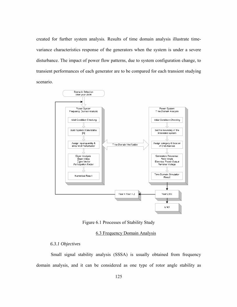
created for further system analysis. Results of time domain analysis illustrate time-
variance characteristics response of the generators when the system is under a severe
disturbance. The impact of power flow patterns, due to system configuration change, to
transient performances of each generator are to be compared for each transient studying
scenario.
Figure 6.1 Processes of Stability Study
6.3 Frequency Domain Analysis
6.3.1 Objectives
Small signal stability analysis (SSSA) is usually obtained from frequency
domain analysis, and it can be considered as one type of rotor angle stability as
125

126
mentioned in chapter 3. The problem usually appears in the form of poorly damped or
undamped oscillations in the system. Since disturbance is assumed to be sufficient small
so that the system can be linearized. Therefore, modal analysis based on eigenvalues
technique is the enabling tool. The main objective of this study is to examine the small
signal stability behavior of the Thailand interconnected system.
6.3.2 Scenarios creation
Since this study examines the Thailand interconnected system from SSSA
perspective, critical modes should be identified for various system loading conditions,
configurations, and contingencies. In this dissertation, a scenario is defined as the
combination of system re-configurations and/or contingencies that change system
operating condition. Based on the available base case data of year 2004, 9 scenarios
have been created to cover configurations change and N-1 contingencies.
In contingencies study, the unavailability of single facility is focused on the
large generation facility near Bangkok area and those heavily loaded lines in the system.
These two types of contingencies have a high potential to cause system instability.
Following are the definition of factors affecting to each scenario.
a) Configuration changes scenario
Scenarios which include changes in loading conditions, generation patterns, and
available transmission lines will refer to as “configuration change scenarios”.
b) Contingencies changes scenario
Scenarios which result from the change in generation patterns and available
transmission lines due to contingencies will refer to as “contingency change scenarios”.

127
6.3.3 Define small perturbation for SSSA
The process of defining location and amount of small perturbation is important
for creation of a system state matrix A. Since SSSA employs the linearized technique
regarding to a small disturbance. This small disturbance can usually be treated as a
small load change or generation level change to balance the load. For simulation
purpose, a small variation of mechanical power input was applied to an online unit near
Bangkok area to create a small perturbation to a system.
Since the main objective of this study is to examine the oscillation modes in
Thailand power system, only complex conjugate eigenvalues will be focused. The
criterions for oscillation modes justification used in this dissertation are as following:
a) Interarea or global mode oscillation
These phenomena involve a group of generators in one area swinging against
another group of generators in another area. The typical oscillation frequency is
approximately 0.1 – 0.4 Hz.
b) Intraarea or local mode oscillation
Generally, local mode oscillation is the behavior of one machine swinging
against the rest of the system. The typical oscillation frequency for this type of
oscillation is approximately 1.0 – 2.0 Hz.
6.3.4 Small signal stability result
6.3.4.1 Interarea or global mode
As mention in section 6.3.2, there are 9 scenarios to be included in this SSSA.
Table 6.1 shows all scenarios and their descriptions.

128
Table 6.1 Scenarios for SSSA and interarea modes of oscillation
Contingencies Interarea Oscillation no. Cases Description Config. change N-1
Gen. N-1 Line
Freq. (Hz)
Damping (%)
Stable Location of
Modes 1 Y04 Base case × × × 0.42 2.78 Yes South1 2 Y04 N-1 Gen × √ × 0.43 2.52 Yes South1 3 Y04 N-1 Line × × √ 0.41 3.68 Yes South1 4 Y06 Normal √ × × 0.36 8.39 Yes South2 5 Y06 N-1 Gen √ √ × 0.42 3.10 Yes South2 6 Y06 N-1 Line √ × √ 0.4 4.73 Yes South2 7 Y08 Normal √ × × 0.41 2.67 Yes South2 8 Y08 N-1 Gen √ √ × 0.44 0.23 Yes South2 9 Y08 N-1 Line √ × √ 0.4 4.3 Yes South2
The 2004 summer peak power flow case is used as a base case. Various
scenarios showing in table 6.1 are result from configurations changes and system
contingencies. The scenario no. 2, Y04 N-1 Gen, referred to as the unavailability of the
largest generation facility in system (in area 7), while scenario no. 3 represents the
absence of the heaviest tie line (between area 6 and Bangkok) in the system. The
creation of these scenarios was intended to investigate the impact of unavailability of a
significant facility on the interarea oscillation mode. Base on the current available data,
when compare result for year 2004, the oscillation frequency for the interarea mode is
approximately 0.41 Hz, with less than 3 percent of system damping. The group of
generator in the southern part is dominant in this mode. System damping for cases of
year 2006 found to be improved when compare to year 2004. The possible reason is the
installation of new units during year 2004 to 2006. However, the unavailability of
largest generator in year 2008 results in the worst case situation with the system
damping at only 0.23 percent. It can be seen for most of cases that major oscillation
modes are located at the southern part of Thailand. In addition, the absence of

129
generation facility deteriorates system damping factor worse than the line does. The
main reason is because the selected base case is the summer peak load which means
generator facilities become very important.
In summary, generators in the southern area have a significant effect on
interarea oscillation modes in Thailand system. The observable oscillation is around 0.4
Hz with less than 4 percent damping factor. In other word, generation plants in the
southern area should be a good location for install power system stabilizers (PSSs). Of
course, further system analysis for PSS’s parameter selection should be performed
before real implementation.
6.3.4.2 Intraarea or local mode
Similar to scenarios in table 6.1, all cases description remain the same yet the
result of table 6.2 focus on intraarea or local oscillation modes. It is found in year 2004
that generators in the central and east part of the country experience intraarea mode with
1.9 Hz of oscillation frequency at around 6.6 percent of damping factor. The same
oscillation frequency was observed for year 2006, but generating units in the northern
happen to encounter with this oscillation problem. It should be noted that, similar to the
trend in interarea mode, the unavailability of any single generation have a tendency of
giving a poor damping to a system when compare to the case of an absence of
transmission lines.

130
Table 6.2 Scenarios for SSSA and intraarea modes of oscillation
Contingencies Interarea Oscillation Freq & Location (1)
Interarea Oscillation Freq & Location (2)
no. Cases Description Config. Change
N-1 Gen.
N-1 Line
Freq. (Hz)
Damping (%)
Freq. (Hz)
Damping (%)
1 Y04 Base case × × × 1.65 East
6.56 1.27 West
6.87
2 Y04 N-1 Gen × √ × 1.93 Central
6.24 1.92 East
6.60
3 Y04 N-1 Line × × √ 1.93 East
6.50 1.92 Central
6.70
4 Y06 Normal √ × × 1.96 North
6.47 1.94 North
6.74
5 Y06 N-1 Gen √ √ × 1.95 North
6.19 1.94 North
6.85
6 Y06 N-1 Line √ × √ 1.96 North
6.40 1.94 North
6.75
7 Y08 Normal √ × × 2.00 East
5.93 1.97 North
6.35
8 Y08 N-1 Gen √ √ × 1.98 East
5.90 1.97 North
6.50
9 Y08 N-1 Line √ × √ 2.00 East
8.25 1.97 North
9.26
6.3.4.3 Observation of worst case scenario
Figure 6.2 is the partial list of the eigenvalues while figure 6.3 shows the
corresponding participation factor of the selected modes. According to result in table
6.1, scenario no. 8 can be considered as a worst case scenario because it has a worst
damping factor of 0.23 percent. As presented in figure 6.2, mode no. 248 is
corresponding to this damping factor. For a selected mode of interest, their top ten
corresponding participation factors are presented in figure 6.3. It is found that the
generator which has a significant effect on mode no. 248 is the generator at bus no.
3051 located in the southern part of the country.

131
a) Eigenvalues result (partial listed)
2008 SUMMER PEAK LOAD PEAK LOAD AT 26048 MW. EIGENVALUES: MODE REAL IMAG DAMP FREQ 1 -2.7044 19.126 0.14000 3.0440 2 -2.7044 -19.126 0.14000 3.0440 3 -2.4607 18.456 0.13216 2.9373 4 -2.4607 -18.456 0.13216 2.9373 5 -1.6889 17.131 0.98115E-01 2.7264 6 -1.6889 -17.131 0.98115E-01 2.7264 7 -2.1624 13.369 0.15967 2.1277 8 -2.1624 -13.369 0.15967 2.1277 9 -0.98878 12.456 0.79132E-01 1.9824 10 -0.98878 -12.456 0.79132E-01 1.9824 11 -1.1242 12.399 0.90299E-01 1.9733 12 -1.1242 -12.399 0.90299E-01 1.9733 13 -1.1241 12.399 0.90297E-01 1.9733 14 -1.1241 -12.399 0.90297E-01 1.9733 ......... ......... 243 -0.33464 4.7672 0.70024E-01 0.75873 244 -0.33464 -4.7672 0.70024E-01 0.75873 245 -0.85413E-01 3.4013 0.25104E-01 0.54133 246 -0.85413E-01 -3.4013 0.25104E-01 0.54133 247 -0.62695E-02 2.7529 0.22774E-02 0.43814 248 -0.62695E-02 -2.7529 0.22774E-02 0.43814
Figure 6.2 Example of eigenvalues result (scenario no.8)

132
b) Modes of interest and top ten participation factor result (partial listed)
2008 SUMMER PEAK LOAD PEAK LOAD AT 26048 MW. NORMALIZED PARTICIPATION FACTORS FOR MODE 248: -0.62695E-02 -2.7529 FACTOR ROW STATE MODEL BUS X-- NAME --X ID 1.00000 198 K+5 GENROU 3051 KA-T1 24.0 1 0.99881 197 K+4 GENROU 3051 KA-T1 24.0 1 0.97928 164 K+5 GENROU 3013 KN-C13 11.5 13 0.97925 152 K+5 GENROU 3011 KN-C11 11.5 11 0.97918 163 K+4 GENROU 3013 KN-C13 11.5 13 0.97918 158 K+5 GENROU 3012 KN-C12 11.5 12 0.97916 151 K+4 GENROU 3011 KN-C11 11.5 11 0.97909 157 K+4 GENROU 3012 KN-C12 11.5 12 0.67472 170 K+5 GENROU 3015 KN-C10 15.0 10 0.67402 169 K+4 GENROU 3015 KN-C10 15.0 10 NORMALIZED PARTICIPATION FACTORS FOR MODE 9: -0.98878 12.456 FACTOR ROW STATE MODEL BUS X-- NAME --X ID 1.00000 433 K+4 GENROU 6001 BPK-T1 22.0 1 0.99985 439 K+4 GENROU 6002 BPK-T2 22.0 2 0.99903 434 K+5 GENROU 6001 BPK-T1 22.0 1 0.99889 440 K+5 GENROU 6002 BPK-T2 22.0 2 0.05605 432 K+3 GENROU 6001 BPK-T1 22.0 1 0.05604 438 K+3 GENROU 6002 BPK-T2 22.0 2 0.03579 430 K+1 GENROU 6001 BPK-T1 22.0 1 0.03579 436 K+1 GENROU 6002 BPK-T2 22.0 2 0.03295 431 K+2 GENROU 6001 BPK-T1 22.0 1 0.03294 437 K+2 GENROU 6002 BPK-T2 22.0 2 NORMALIZED PARTICIPATION FACTORS FOR MODE 10: -0.98878 -12.456 FACTOR ROW STATE MODEL BUS X-- NAME --X ID 1.00000 433 K+4 GENROU 6001 BPK-T1 22.0 1 0.99985 439 K+4 GENROU 6002 BPK-T2 22.0 2 0.99903 434 K+5 GENROU 6001 BPK-T1 22.0 1 0.99889 440 K+5 GENROU 6002 BPK-T2 22.0 2 0.05605 432 K+3 GENROU 6001 BPK-T1 22.0 1 0.05604 438 K+3 GENROU 6002 BPK-T2 22.0 2 0.03579 430 K+1 GENROU 6001 BPK-T1 22.0 1 0.03579 436 K+1 GENROU 6002 BPK-T2 22.0 2 0.03295 431 K+2 GENROU 6001 BPK-T1 22.0 1 0.03294 437 K+2 GENROU 6002 BPK-T2 22.0 2
Figure 6.3 Participation Factor Result of interested modes

133
6.4 Time Domain Analysis
6.4.1 Objectives
Transient stability analysis was performed to determine the potential stability
problems due to system configurations changed following severe disturbances. The
transmission line base case model used in this study was the 2004 summer peak
condition. Main objective of this transient stability study is to examine the system
response, especially for important generation units, following a severe disturbance. This
process is accomplished by time domain simulation technique.
6.4.2 Scenarios creation
Similar to processes in SSSA, this transient stability study shall be performed
for various system loading conditions, configurations, and contingencies. A scenario is
defined as a combination of configuration changes and/or contingencies that alter
system operating condition. Based on the available base case data and the creation of
two subsequent years, 18 scenarios were created and compared the result. Similar to the
SSSA, same terms of factor affecting each scenario were adopted for this transient
study.
a) Configuration changes scenario
Scenarios which include changes in loading condition, generation patterns, and
available transmission lines will refer to as “configuration change scenarios”.
b) Contingencies changes scenario
Scenarios which result from the change in generation patterns and available
transmission lines due to contingencies will refer to as “contingency change scenarios”.

134
6.4.3 Define severe disturbances for TSA
Various system configurations and faults were considered to determine the
possible stability issues. In this dissertation, similar to typical standard simulation for a
severe disturbance, a 5 cycle three-phase fault is deployed for the study cases.
Followings are two main types of disturbances focused in this study.
a) The unavailability of single generation facility is focused on the outage of two
main generation units. The first one is the unit in the load center (Bangkok) and another
one is the largest generator in the system (in area 7). The disturbances were based on a
5-cycles three-phase fault on those two generators’ buses followed by tripping the unit
for the system protection.
b) Another contingency is concentrated on the outage of heaviest tie line
following critical disturbances. The disturbance was also based on a 5-cycles three-
phase fault on the line followed by removing the fault through tripping the line.
6.4.4 Transient stability result
6.4.4.1 Scenarios summary
As mention in section 6.4.2, there are 18 scenarios to be included in this TSA.
Table 6.3 shows all cases study (scenarios) and their disturbances’ description including
summary of transient simulation result

135
Table 6.3 List of studied scenarios for TSA
Types of Disturbances no. Cases Description Configu-ration change
Gen1 Fault
Gen1 Fault &
Trip
Gen2 Fault
Gen2 Fault &
Trip
Tie line Fault &
Trip
System Stable?
1 Y04 Base case × Yes 2 Y04 Fault 1 × √ Yes 3 Y04 Fault 2 × √ Yes 4 Y04 Fault 3 × √ Yes 5 Y04 Fault 4 × √ Yes 6 Y04 Fault 5 × √ Yes 7 Y06 Base case √ Yes 8 Y06 Fault 1 √ √ Yes 9 Y06 Fault 2 √ √ Yes
10 Y06 Fault 3 √ √ Yes 11 Y06 Fault 4 √ √ Yes 12 Y06 Fault 5 √ √ Yes 13 Y08 Base case √ Yes 14 Y08 Fault 1 √ √ Yes 15 Y08 Fault 2 √ √ Yes 16 Y08 Fault 3 √ √ Yes 17 Y08 Fault 4 √ √ Yes 18 Y08 Fault 5 √ √ Yes
Base on available data of the 2004 peak summer load and the result of different
traditional dispatching patterns from chapter 5, the first stability case is “Y04 Base
case”. The reason to generate scenario no.1 (table 6.3) is to assure the accuracy of initial
condition of the system. For each studied case, to guarantee if there is enough time for
system to achieve the new equilibrium after disturbance, the extended simulation time
to 15 seconds was performed.
It is clear from table 6.3 that power system can regain to the new equilibrium
point following disturbance in most of studied cases. The following sections show
simulation results and detail discussions regarding to scenarios in table 6.3.

6.4.4.2 Time domain simulation result for year 2004
Showing in figure 6.4 to 6.9 are time domain simulation results for year 2004
scenarios. As a basic rule, initial condition checking is a pre-requisite. Showing in
figure 6.4, power output of 6 generation units located in the metropolitan, eastern,
western, northern, central, and southern areas are monitored. This dissertation will
monitor these 6 units for all the transient stability study cases.
Figure 6.4 Initial condition checks for TSA (2004)
From figure 6.4, one can see that all generation units are in the equilibrium
initial condition. It should be noted that the largest generation delivers 520 MW for the
peak demand of year 2004.
136

Figure 6.5 Momentary fault at a generator in load center area (2004)
Figure 6.5 is the response of the system due to a momentary fault at a generator
bus near the load center. The power swings decay very quick which indicate a good
system damping. The system can still regain to the new equilibrium point if this
particular generator has experienced with a permanent fault and is taken out of service.
However, as shown in figure 6.6, two units from the eastern and western area deliver
more power to make up the generation deficiency due to the tripping of a generation
unit at the load center.
137

Figure 6.6 Fault at a generator in load center area followed by unit trip (2004)
In figure 6.7, a temporally fault at the largest generation unit gives a more
severe oscillation of power output compare to the figure 6.5. This is because the largest
generation can have a more contribution in fault current. In other word, it has a higher
potential to create a more unbalance situation to the system. In figure 6.8, it can be seen
that the similar trend of two units in eastern and western area deliver more power to
make up the generation deficiency due to the tripping of a largest generation unit in area
7.
138

Figure 6.7 Momentary fault at a largest generator (2004)
Figure 6.8 Fault at a largest generator followed by unit trip (2004)
139

Figure 6.9 Fault at a heaviest loading tie line followed by line trip (2004)
The last case for transient stability case of year 2004 is the response of system
when a severe disturbance happens at the heaviest tie line following trip the line to clear
the fault. Showing in figure 6.9, it is found that this case create more oscillation to
system when compare with previous cases. However, the system can still recover to the
new stable point in approximately 12 seconds.
140

6.4.4.3 Time domain simulation result for year 2006 and 2008
The simulation result for the year 2006 and 2008 are basically the same trend as
presented in year 2004. The observable difference is an output level of the units. At the
normal operating condition, output power delivered from the largest unit of year 2004,
2006 and 2008 are at 520 MW, 560 MW, and 720 MW respectively. This situation
causes the higher amplitude of oscillation for those cases in year 2008 compare to those
cases in year 2004. Time domain simulation result for all cases in year 2008 can be
found in figure 6.10 – 6.15.
Figure 6.10 Initial condition checks for TSA (2008)
141

Figure 6.11 Momentary fault at a generator in load center area (2008)
Figure 6.12 Fault at a generator in load center area followed by unit trip (2008)
142

Figure 6.13 Momentary fault at a largest generator (2008)
Figure 6.14 Fault at a largest generator followed by unit trip (2008)
143

Figure 6.15 Fault at a heaviest tie line followed by line trip (2008)
144

145
6.5 Chapter summary
Frequency domain analysis or small signal analysis is first performed in this
chapter. The main objective is to examine the possible low frequency oscillation mode
in Thailand system. Throughout the whole study, there is no positive complex
eigenvalue emerge on the right side of S-plan. However, there is potential interarea low
frequency oscillation at 0.4 Hz with damping factor less than 4 percent. Most of the
cases, generators in the southern area have more influence on interarea oscillation
modes. The critical scenario is observed when the largest generation unit is tripped in
year 2008. According to the simulation results, system will experience a relatively poor
damping factor of 0.23 percent.
Time domain analysis was performed to determine the potential stability
problems that can be originated by the system configurations changed following severe
disturbances. There are five categories of disturbance of interest. Base on the available
actual data of year 2004, and study result from chapter 5, it is found that system can
regain to the new equilibrium condition following severe disturbances.
In conclusion, base on the available data of summer peak 2004 case, all stability
study results in both frequency domain and time domain analysis for Thailand power
system indicate that Thailand power system still has a stability safety margin until 2008.
Simulation results reveal that the unavailability of generation facilities can cause more
severe problem to system than transmission facility does.

146
CHAPTER 7
VISION FOR ELECTRICITY SUPPLY INDUSTRY OF THAILAND
7.1 Introduction
Since 1998, right after the economic crisis, the cabinet of Thailand approved a
master plan for privatization of state enterprises in fours sectors including energy sector.
Similar to any other businesses agency, the electricity supply industry in Thailand have
to perform a comprehensive study not only a technical side but also a financial aspect to
assure the minimum impact from this privatization and/or transformation planning. The
concerns for demand side are more important for the government because the new
operation structure may fail or may be difficult to implement without the acceptance
from the customers in the country.
The main objective of this chapter is to propose a possible procedure as a
decision tool to determine the proper timing for the new operating paradigm. The
possible framework for ESI structure is also recommended. In this dissertation, two
main justifications for the transformation are proposed. The first one is based on system
security, and second one is economic and financial justification. As stated in chapter 3,
security assessment is the pre-requisite before any paradigm change. Therefore, before
any deregulation activities take action, system-wide operation conditions have to meet
minimum security requirements as discussed in chapter 4 and 6. The economic and

147
financial analysis is then become the second significant issue. Usually, the financial
incentive is the most powerful tool for controlling all market participants (MPs). Any
strong objection, or support for the new market structure will depend directly on the
financial impact to MPs. It should be noted that the more acceptance from MPs, the
better the possibility to success in the new operation paradigm.
To accomplish the objective function, this dissertation classifies two types of
market participants (players) in Thailand power system for the purpose of the
justification. It should be noted that this procedure is only to determine when to
transform the system to the new environment. Later, different participants’ rights and
roles have to be re-defined by the regulatory before the new structure can be operated.
In this manner, player 1 is the electricity supply side which refers to the Electricity
Generating Authority of Thailand (EGAT). The second player is the demand side which
refers to as the electricity consumers in the whole country.
This chapter deploys the economic concept to identify a proper transformation
year to new market environment. It should be the year where the equilibrium between
both players in the system is met. From the perspective of supply side, the concept of
marginal analysis will be used as a decision-tool for answer this question. For demand
side, result of generation dispatching costs from chapter 5 which directly reflect their
electricity bill, will be used as an indicator to decide when to enter the new market
operation. It needs to reach an optimization condition between these two parties because
they hold the responsibilities for power system security operation and financial
obligation for all MPs. Therefore, the game theory is utilized for creating the

148
transformation matrix. This matrix reasonably determines the proper timing for a
smooth transformation.
7.2 Marginal Analysis (An Economy Index for a supply side)
It is to be noted that this marginal analysis is based on financial aspect of the
supply side only. The consideration of technical part is excluded. Historical data from
EGAT annual reports [60], energy consumption forecasted data from EPPO including
the trend of fuel cost for electricity generation are main sources of this analysis. Since
the final ruling requires more extensive analysis, results from this study only provide a
general recommendation procedure for the study.
7.2.1 Basic assumptions
Three main assumptions are required before accomplishing the study processes.
a) EGAT as a monopoly in ESI structure
In economic theory, there are usually four main types of market structure as
shown in figure 7.1. They composed of monopoly, oligopoly, monopolistic competition,
and perfect competition. The marginal analysis can be more successful when applying
to the monopoly market structure rather than the others. Historical data from EGAT’s
annual reports show that EGAT has produced more than 60 percent of total energy
consumption in the whole country at the present time. In addition, with the power
purchase agreement (PPAs), EGAT has the right to buy produced-energy from other
IPPs and SPPs and then resell them to other customers. In this respect, EGAT is the
single buyer in the system. Therefore, this dissertation considers EGAT as a monopoly
in the electricity supply industry in Thailand system.

Figure 7.1 Four different types of market structure
b) Electricity generation department is dominance
Though there are many sub-organizations and departments inside EGAT, the
electricity generation department is considered as the most significant division because
more than 90 percent of EGAT total revenue is generated from this department.
Therefore, this dissertation will treat this department as one independent business
organization and its ultimate goal is profit maximization.
c) Other correlated considerations
Usually, there are many factors related to financial analysis for any business
organization. This dissertation tries to simplify the calculation analysis yet still obtain
the reasonable result. Therefore, other related assumptions were included prior to have a
final result in table 7.1. The following are of those considerations.
c.1 Demand forecast is based on the 2004 EPPO load forecast subcommittee.
The demand growth rate is approximately 7% per year according to MEG.
c.2 The calculation of total revenue (TR) is based on EGAT average selling
price to customer, assuming that this selling price is 5% increasing each year.
c.3 Four types of fuel cost are used for estimating EGAT’s total generation cost.
They composed of natural gas (NG), fuel oil (FO), lignite (LN), and diesel oil (DO).
c.4 Considering total cost (TC) of electricity generation department, there are
two main cost components i.e. electricity generation cost and administration cost. 149

150
Electricity generation cost composed of four cost components, which are purchase
energy cost (55%), fuel cost (30%), generation cost (10%) and transmission cost (5%).
c.5 The cost of hydro units can be covered by the difference between revenue
from selling power and expense from purchasing power from IPPs and SPPs.
c.6 According to ten years planning in PDP 03-04, starting at year 2003, EGAT
plans to reduce the market share of its own generation from 50% down to 42% at the
end of year 2011. This action implies 1% declining in generation capacity each year.
c.7 Though lignite provides the least expensive generation cost (0.75 – 1.0
cent/kWh), almost of new generation units will base on the natural gas (2.0 – 2.5
cents/kWh) due to the economic and environmental reasons (PDP 04).
Based on these assumptions, complete marginal analysis result both in
numerical and graphic format are presented in the following sections.
7.2.2 Study results
Table 7.1 shows the financial result after performing marginal analysis. It can be
observed that EGAT can maximize net profit when its marginal revenue is equal to its
marginal cost. Theoretically (refer to chapter 3), the marginal revenue is defined as “the
change in total revenue that are derived from undertaking some economic activity”,
while marginal cost is defined as “the change in total cost that occurs from undertaking
some economic activity”. Ideally, if marginal revenue still greater than marginal cost,
this situation imply the expansion of an economic activity. On the other hand, when
marginal revenue is less than marginal cost, the downsizing of economic activity should

151
be applied. However, if they are equal, it reaches the stage of profit maximization.
Therefore, the business organization should maintain their current economic status.
Table 7.1 Marginal analysis result (supply perspective)
Fiscal Year Energy Demand Forecast (M kWh)
Estimated Total
Revenue
(M Baht)
Estimated Total Cost
(M Baht)
Marginal Revenue
(M Baht)
Marginal Cost
(M Baht)
2000 98536 160240.49 111615.31 - - 2001 103868 185509.49 131557.09 25269 19941 2002 111299 211335.87 154320.42 25826 22763 2003 118374 231445.23 180182.91 20109 25862 2004 126811 257477.05 203201.24 26031 23018 2005 136784 288012.39 232840.01 30535 29638 2006 147658 322012.56 266482.74 34000 33642 2007 158212 356926.30 302160.40 34913 35677 2008 169280 394625.50 341538.10 37699 39377 2009 180942 435418.80 385039.50 40793 43501 2010 193530 480264.00 433697.50 44845 48658
From the supply perspective, results from table 7.1 imply that EGAT should
modify their operation strategy after year 2007 because its marginal revenue will fall
below marginal cost. Figure 7.2 show the graphical result of estimated EGAT total
revenue and total cost, while figure 7.3 presents the marginal analysis result.

Forecasted EGAT total Revenue and total cost
0
100
200
300
400
500
600
2000 2001 2002 2003 2004 2005 2006 2007 2008 2009 2010
Thou
sand
s
Year
Bah
t
Total Rev.
Total Cost
Figure 7.2 EGAT total revenue and total cost estimation
Marginal Analysis
0
10
20
30
40
50
60
2001 2002 2003 2004 2005 2006 2007 2008 2009 2010
Thou
sand
s
Year
Bah
t
MarginalRev.MarginalCost
Figure 7.3 Marginal analysis graphical results
Additional discussions on the marginal analysis focus on factors that could have
significant impact on the result. The analysis outcomes were presented in figure 7.4 and
7.5. In figure 7.4, if EGAT could have a re-engineering process within its organization,
152

the administration cost and depreciation cost can be reduced. Thus, it is found from
figure 7.4 that EGAT can delay process of transformation from year 2007 to year 2009.
Marginal Analysis (exclude admin & depreciation)
05
101520253035404550
2001 2002 2003 2004 2005 2006 2007 2008 2009 2010
Thou
sand
s
Year
Bah
t
MarginalRevMarginalCost
Figure 7.4 Marginal analysis graphical result (exclude administration cost)
However, due to majority of EGAT expense is come from the fuel cost, these
fuels cost depend the foreign factors such as supply and demand, world economy
situation etc. In other word, these factors are uncontrollable and they can be considered
as uncertainty factors. Therefore, taking into account the uncertainty of fuel cost, result
of marginal analysis can be obtained in a more conservative fashion. If the fuel cost is
increasing 5% more than expected value, year 2008 is the optimal year for EGAT to
modify their operation strategy to maintain the ultimate economic goal.
153

Marginal Analysis (5% increasing in Fuel Cost from 2004)
05
101520253035404550
2001 2002 2003 2004 2005 2006 2007 2008 2009 2010
Thou
sand
s
Year
Bah
t
MarginalRev.MarginalCost
Figure 7.5 Marginal analysis graphical result (include effect of uncertainty in fuel cost)
7.3 Game theory (A transformation matrix)
One of the powerful tools in economic strategy is the game theory. The main
idea is to identify the equilibrium situation or solution among several players in the
game. As discuss in chapter 3, the arrow technique is utilized in this dissertation due to
its simplicity yet powerful characteristic for determining optimal strategy. Usually,
many situations can happen among players in the game. Dominant strategy seems to be
the easiest way to identify the solution. On the other hand, if there is existing more than
one dominant solution in some game, then the concept of Nash equilibrium can be used
to handle this situation.
7.3.1 Basic assumptions
It is first assumed a two-player game during a decision stage to determine the
timing to transform the ESI structure in Thailand. This dissertation applies the concept
of payoff table in game theory to create the so called “transformation matrix”. The
154
155
purpose of such matrix is to identify the optimal year for both players in Thailand
system for a smooth transition to the new environment. Final result of this problem can
be found in table 7.2 to 7.4. Since the result of this game will create a direct impact to
all MPs in Thailand, it is recommended that dominant strategy should be the best
solution for this game.
7.3.2 Define payoff for each player
The most significant component in creating transformation (payoff) matrix is to
find the payoff for each player. It is found that the common indicator which can
represent payoff for both players is their satisfied level. In this dissertation, payoff for
each player is defined as the level of satisfaction corresponding to their financial
obligation. Following are considerations for assigning payoff to each player.
7.3.2.1 Payoff for the supply side
In this respect, the supply side is referred to as EGAT who is a single buyer in
Thailand system. The marginal analysis result from section 7.1 concludes that EGAT
should modify their operation strategy at year 2008. This situation implies that before
year 2008, EGAT satisfies with their traditional operation due to their MR is greater
than MC. Therefore, if EGAT keeps staying in the same course, thus their payoff is
equal to 1 (satisfy). In other word, if EGAT has to move to the new operation strategy
before year 2008, its payoff will be -1 (dissatisfy). However, after year 2008, the
situation is reversed. EGAT will be satisfied under the deregulated environment because
they can accomplish their profit maximization. Whereas, if EGAT stay in the traditional
operation, they will generate less profit yield the dissatisfy situation.

156
7.3.2.2 Payoff for the demand side
This dissertation assumes that the financial obligation of electricity consumers
depend on the total cost of electricity generation from EGAT. Therefore, the generation
pattern that offer the least generation cost will provide the highest level of satisfaction
for consumers. From the system-wide viewpoint, the least electricity generation cost
yield the maximizing in social welfare. The generation cost resulted from different
dispatching patterns in chapter 5 will be the significant indicator for the demand side to
find their willingness time frame to accept the new operation paradigm. Result from
table 5.11 and 5.12 reveal that under deregulated environment, ISO/SO utilizes optimal
power flow (OPF) to find the optimal generation dispatching patterns. As a result, better
instruction dispatching patterns (cheaper in generation cost) were accomplished.
Therefore, for demand side, as soon as the time of implementing new environment, they
should have more benefits when compare to the traditional operation. These benefits
may include the lower in electricity price, more choices of electricity supplier, and
better service quality. Thus, according to the result in chapter 5, year 2006 should be the
first year for demand side to feel comfortable to accept the new operation environment.
This situation means that the payoff for demand side should be 1 (satisfy) after year
2006 if the new operation strategy successfully implemented. On the other hand, -1
(dissatisfy) should be assigned in the payoff matrix for demand side if traditional
operation still valid.

157
7.3.3 Study results
Based on all economic assumptions, technical considerations, and defined
payoff values, these factors can be used to form the transformation matrix as shown in
table 7.2 to table 7.4. Table 7.2 shows the transformation matrix of year 2004. It is clear
that player 1 (supply) will choose traditional operation strategy because it gives a better
payoff for them. Whereas, player 2 (demand) will prefer the deregulation environment
due to the lower in electricity price. As a result, there is no equilibrium result between
these two players.
Table 7.2 Transformation table (year 2004 payoff table)
Demand Player 2
Year 2004
Traditional Deregulation Traditional
1 -1 1 1
Supply Player 1
Deregulation -1 -1 -1 1
Table 7.3 is transformation matrix for year 2006. It can be found that the same
payoff for both players as in a year 2004. Therefore, there is also no dominant solution
for this year either.
Table 7.3 Transformation table (year 2006 payoff table)
Demand Player 2
Year 2006
Traditional Deregulation Traditional
1 -1 1 1
Supply Player 1
Deregulation -1 -1 -1 1

158
Unlike previous years result, payoff table for year 2008 reveals that supply side
is willing to move to deregulated environment, while demand side also feels
comfortable to accept the new deregulated market. Therefore, the dominant strategy
was found. Applying arrow technique, it is clear that both players will get 1 (satisfy) for
their payoff. This situation creates dominant strategy to be an optimal solution for
Thailand system.
Table 7.4 Transformation table (year 2008 payoff table)
Demand Player 2
Year 2008
Traditional Deregulation Traditional
-1 -1 -1 1
Supply Player 1
Deregulation 1 -1 1 1
In conclusion, the equilibrium year for both players of this game should be in
the year 2008 because both players accomplish their level of satisfaction. However,
others concerns of secure operation considerations, operation frameworks, possible
settlement processes should be addressed before the real implementation of the new
system. The following section proposes and discusses the possible operation framework
by taking into account all the relevant limitations including social concerns in Thailand
system. Summarized table of the recommendation framework is presented in table 7.5

159
7.4 The operation framework recommendation for ESI restructuring in Thailand during the transition stage
Although transmission congestion management (TCM) issue has been widely
debated for the decade, it is still an opened issue extensively discussed in the current
competitive environment. For Thailand, the processes of restructuring of Electricity
Supply Industry is still under the beginning phase, many concerns, such as advance in
an information technology, energy security, social equity, price volatility, and the need
to subsidize poor consumers, are necessary to be considered before the establishment of
TCM and settlement processes.
Taking into account the gross income disparity among the population, social
equity policy should and would be pursued by the government. In this respect, equitable
access to electricity irrespective of geographical location is desirable and the need to
subsidy for lower income groups should still be implemented. In addition, the current
structure of OASIS, computer information technology including the high speed internet
services is still under the developing stage. It may take a while for Thailand to fully
upgrading the computer information technology especially the high speed internet to
support the operation requirement (OASIS) under competitive environment.
Following section summarizes the proposed recommendation framework for the
utility industry deregulation processes in Thailand. For simplicity, this summary will
base upon FERC’s standard market design (SMD), and market design of ERCOT.
Table 7.5 presents the proposed framework of ESI structure during the transition
period in Thailand. The first recommended market element is about the requirement of
balancing schedule. This element creates more confident in operation and control for
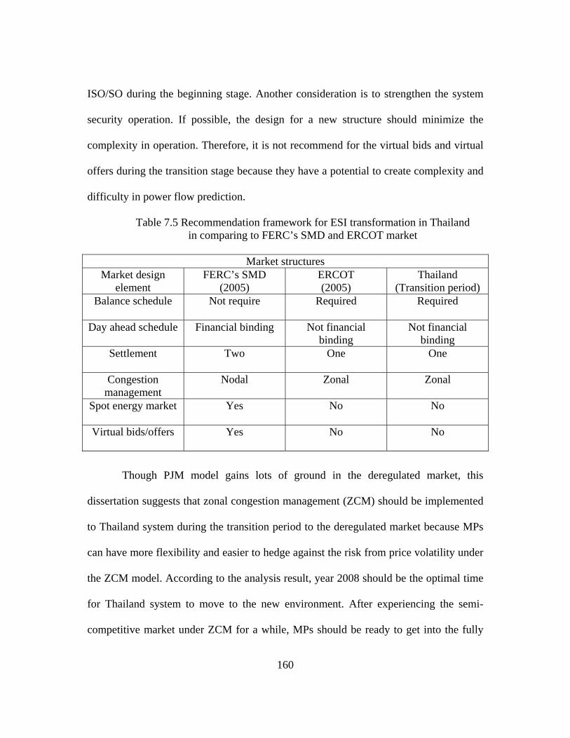
160
ISO/SO during the beginning stage. Another consideration is to strengthen the system
security operation. If possible, the design for a new structure should minimize the
complexity in operation. Therefore, it is not recommend for the virtual bids and virtual
offers during the transition stage because they have a potential to create complexity and
difficulty in power flow prediction.
Table 7.5 Recommendation framework for ESI transformation in Thailand in comparing to FERC’s SMD and ERCOT market
Market structures
Market design element
FERC’s SMD (2005)
ERCOT (2005)
Thailand (Transition period)
Balance schedule
Not require Required Required
Day ahead schedule Financial binding Not financial binding
Not financial binding
Settlement
Two One One
Congestion management
Nodal Zonal Zonal
Spot energy market
Yes No No
Virtual bids/offers
Yes No No
Though PJM model gains lots of ground in the deregulated market, this
dissertation suggests that zonal congestion management (ZCM) should be implemented
to Thailand system during the transition period to the deregulated market because MPs
can have more flexibility and easier to hedge against the risk from price volatility under
the ZCM model. According to the analysis result, year 2008 should be the optimal time
for Thailand system to move to the new environment. After experiencing the semi-
competitive market under ZCM for a while, MPs should be ready to get into the fully

161
competitive environment in which Nodal congestion management (NCM) would be
employed in the TCM process due to a superior in accurate indicating for future system
expansion and planning.

162
CHAPTER 8
CONCLUSION
Transmission congestion management (TCM) issue has been widely debated
during the past decade. It is still an opened issue extensively discussed in the current
competitive environment. In the United State, PJM with nodal congestion management
(NCM) base on renowned location marginal price (LMP) and the Electric Reliability
Council of Texas (ERCOT) with zonal congestion management (ZCM) are two
successful stories of TCM under different operation schemes. Though PJM model is
adopted in some developing countries where the processes of restructuring of Electricity
Supply Industry (ESI) is still under the beginning phase, many concerns, such as
advance in an information technology, energy security, social equity, price volatility,
and the need to subsidize poor consumers, are necessary to be considered before the
establishment of TCM and settlement processes.
For Thailand, as a developing country with the gross income disparity among
the population, social equity policy should and would be pursued by the government. In
this respect, equitable access to electricity irrespective of geographical location is
desirable and some form of subsidy for lower income groups should still be
implemented. In addition, the current structure of OASIS, computer information
technology including the high speed internet services is still under the developing stage.

163
Taking into account the above concerns, this dissertation proposes the
recommendation framework for transmission congestion management scheme that
would be possible to implement in Thailand during its transformation to deregulated
environment. Although NCM model gains lots of ground in the deregulated market
better than ZCM model, price uncertainties at different locations can complicate the
situations. From the conservative viewpoint, ZCM would be a better starting tool for
managing congestion in Thailand system. Adopting the concept from ERCOT, this
dissertation proposes four sequential steps to define the congestion zones for the entire
system. After the transition period, NCM should be utilized for the fully competitive
environment due to its theoretically sound and ability to accurately reflect the operation
conditions of the system.
8.1 Contributions
It is believed that this dissertation will be the first comprehensive study
addressing to Electricity Supply Industry (ESI) deregulation in Thailand. Though some
of proposed concepts and pre-assumptions might not be complete due to realities
situations require more update and more precisely data. In addition, operation rules and
operation situations may be different from reported in this dissertation. Therefore
overall detail process may need to carry out by committee which can be composed of
the Government, EPPO, EGAT, stakeholders, and academia. Since the main objective
of this dissertation is to help the transition from current traditional operation to the new
deregulated environment go smoothly in Thailand, therefore all the frameworks, system

164
security study result, and economic and financial study result reported in this
dissertation make the following contributions to ESI deregulation in Thailand system.
a) Main contribution is the proposed framework study for ESI deregulation in
Thailand system which integrating both security and economy concerns into proposed
framework. This study framework can be applied to other systems which trying to move
to the new deregulated environment.
b) The defined and proposed ISO/RTO’s role, responsibilities, and operation
function in the new deregulated environment. This is including the proposed idea of two
market settlement for the transition stage in Thailand.
c) Security study for a long term planning in Thailand system has been
implemented in both time domain and frequency domain analysis. The detail analysis of
system stability both from a severe disturbance and small signal disturbance can help
SOs to understand and beware the system weak point. This study result also gives the
idea to SOs for a location to install PSS devices or others system protection devices.
8.2 Possible Future Researches
Since this dissertation provide the recommendation guideline and framework in
the deregulated issue in Thailand. There still have a plenty room of research related area
for other scholars which can be partial listed as followed:
a) The detail development of TCM scheme and the settlement processes.
b) Development of SCUC and SCED process to optimize system cost
c) The technique to calculate LMPs including the effect of system losses

165
d) The optimization of DA energy market together with an ancillary service
market.
e) System state estimation for determine real time Available Transfer
Capability (ATC).
f) Reactive power dispatching and control under the deregulated environment.
g) The study of interconnection of new generation facility to improve a
reliability of the system.

REFERENCES
[1] Hugh Rudnick, “The Electricity Market Restructuring in South America: Successes and Failures on Market Design”, Plenary Session, Harvard Electricity Policy Group, presented in San Diego CA, Jan. 29-30, 1998, page(s): 1 – 7.
[2] M. Ilic, F. Galiana and L. Fink. 1998 Power Systems Restructuring: Engineering
& Economics., 10-200. Kluwer Academic Publishers. [3] Electric Power Research Institute. 1999. Real and Reactive Power Tracing: Proof
of Concept and Fesibility Study., 7-30. EPRI Press. [4] California Independent System Operator (Cal-ISO). 1996. What is the California
Independent System Operator (Cal-ISO) Organization Information [available online] http://www.caiso.com/
[5] Richard D. Christie, Bruce F. Wollenberg, and IVAR WANGENSTEEN,
“Transmission Management in the Deregulated Environment”, Invited Paper, Proceeding of the IEEE, Vol. 88, no. 2, February 2000, page(s): 170 – 195.
[6] W.J. Lee, and C.H. Lin, “Utility Deregulation and Its Impact on the Industrial
Power System,” IEEE I&CPS 1997 Annual Conference, 11-16 May 1997, page(s): 217 – 222.
[7] Harry Singh, Shangyou Hao, and Alex Papalexopoulos, “Transmission
Congestion Management in Competitive Electricity Markets”, IEEE Transaction on Power Systems, vol. 13, No.2, May 1998, page(s): 672 – 680.
[8] R.S. Fang and A.K David, “Transmission Congestion Management in an
Electricity Market”, IEEE Transaction on Power Systems, vol. 14, No.3, August 1999, page(s): 877 – 883
[9] Le Anh Tuan, Kankar Bhattacharya, and Jaap Daalder, “A Review on Congestion
Management Methods in Deregulated Electricity Markets”, IEEE Proceeding of Power and Energy System, PES 2004 at Clear Water Beach, FL, Nov 28 – Dec 1, 2004.
166

[10] “Promoting Wholesale Competition Through Open Access Non-Discriminatory Transmission Services by Public Utilities and Recovery of Stranded Costs by Public Utilities and Transmitting Utilities”, Order no.888, 61 FR 21, 540, May 10, 1996.
[11] “Open Access Same-Time Information System (Formerly Real-Time Information
Networks) and Standards of Conduct”, Order no.889, 61 FR 21, 737, May 10, 1996.
[12] Ebrahim Vaahedi and Mohammad Shahidehpour, “Decision Support Tools in
Restructured Electricity Systems: An Overview”, IEEE Transaction on Power Systems, vol. xx, no. xxxx, month 2004, page(s): 1 – 7.
[13] Xingwang ma, David I. Sun, and Kwok W. Cheung, “Evolution Toward
Standardized Market Design”, IEEE Transaction on Power Systems, vol. 18, no. 2, May 2003, page(s): 460 – 469.
[14] Guillermo D.Irisarri, James R. Latimer, et al., “The Future of Electronic
Scheduling and Congestion Management in North America”, IEEE Transaction on Power Systems, vol.18, no. 2, May 2003, page(s): 444 – 451.
[15] B. J. Kirby, J.W. Van Dyke Oak Ridge National Laboratory and C. Martinez,
A.Rodriguez Southern California Edison, “Congestion Management Requirements, Methods and Performance Indices”, ORNL/TM-2002/119, June 2002, page(s): 1-31.
[16] Roberto Mendez and Hugh Rudnick, “Congestion Management and Transmission
Rights in Centralized Electric Markets”, IEEE Transaction on Power Systems, vol. 19, no. 2, May 2004, page(s): 889 – 896.
[17] Minghai Liu, and George Gross, “Framework for the Design and Analysis of
Congestion Revenue Rights”, IEEE Transaction on Power Systems, vol. 19, no. 1, February 2004, page(s): 243 – 251.
[18] Luonan Chen, Hideki Suzuki, Tsunehisa Wachi, and Yukihiro Shimura,
“Components of Nodal Prices for Electric Power Systems”, IEEE Transaction on Power Systems, vol. 17, no. 1, February 2002, page (s): 41 – 49.
[19] Ashwani Kumar, S.C. Srivastava, and S.N.Singh, “A Zonal Congestion
Management Approach Using Real and Reactive Power Rescheduling”, IEEE Transaction on Power Systems, vol. 19, no.1, February 2004, page(s): 554 – 562.
167

[20] Xing Wang and Y.H.Song, “Apply Lagrangian Relaxation to Multi-Zone Congestion Management”, IEEE PES winter meeting 2001, vol 2, 28 Jan. – 1 Feb. 2001, page (s): 399 – 404.
[21] Jun Yu, “ERCOT Zonal Congestion Management”, IEEE Conference paper, PES
Summer Meeting 2002, vol. 3, 21-25 July 2002, page(s): 1339 – 1344. [22] Jun Yu, “Market Solution in ERCOT Balancing Energy Market”, IEEE
Conference paper, PES Summer Meeting 2002, vol. 3, 21-25 July 2002, page(s): 1348 – 1353.
[23] Prabha Kundar and IEEE/CIGRE Joint Task Force, “Definition and Classification
of Power System Stability”, IEEE Transaction on Power Systems, July 8, 2004, page(s): 1 – 15.
[24] D.Y Wong, G.J. Rogers, B. Porretta, and P. Kundur, “Eigen Analysis of Very
Large Power Systems”, IEEE Transaction on Power System, vol. 3, no. 2, May 1988, page(s): 472 – 480.
[25] Power System Dynamic Performance Committee, “Damping Representation for
Power System Stability Studies”, IEEE Transaction on Power System, Vol. 14, no. 1, February 1999, page (s): 151 – 157.
[26] Wei-Jen Lee, Mo-Shing Chen, Jae-Hyeon Gim, Kenji Yoshimura and S. Ping
Wang, “Dynamic Stability Analysis of an Industrial Power System”, IEEE Transaction on Industrial Application, vol. 31, no. 4, July/August 1995, page(s): 675 – 681.
[27] G. Angelidis, and A. Semlyen, “Improved Methodologies for the Calculation of
Critical Eigenvalues in Small Signal Stability Analysis”, IEEE Transaction on Power System, vol. 11, no. 3, August 1996, page(s): 1209 – 1217.
[28] Lei Wang, Meir Klein, S. Yirga, and P. Kundur, “Dynamic Reduction of Large
Power System for Stability Studies”, IEEE Transaction on Power System, vol. 12, no. 2, May 1997, page(s): 889 – 895.
[29] Lei Wang and Kip Morison Powertech Labs Inc., “Small Signal Stability Analysis
and Power System Stabilizer Tuning For ERCOT”, Final Report, January 2002, page(s): 1 – 81.
168

[30] C.Y. Chung, Lei Wang, F. Howell, and P. Kundur, “Generation Rescheduling Methods to Improve Power Transfer Capability Constrained by Small-Signal Stability”, IEEE Transaction on Power System, vol. 19, no. 1, February 2004, page(s): 524 – 530.
[31] Kumar David and Xujun Lin, “Dynamic Security Enhancement in Power-Market
Systems”, IEEE Transaction on Power Systems, vol. 17, no. 2, May 2002, page(s): 431 – 438.
[32] B. Changaroon, S. C. Srivastava, and D. Thukaram, “A Neural Network Based
Power System Stabilizer Suitable for On-Line Training – A Practical Case Study for EGAT System”, IEEE Transaction on Energy Conversion, Vol. 15, no. 1, March 2000, page(s): 103 – 109.
[33] W. Ongsakul, and Nit Petcharaks, “Unit Commitment by Enhanced Adaptive
Lagrangian Relaxation”, IEEE Transaction on Power Systems, Vol. 19, no. 1, February 2004, page(s): 620 – 628.
[34] Wei-Jen Lee, C.H.Lin, and Larry D.Swift, “Wheeling Charge Under a
Deregulated Environment”, IEEE Transaction on Industry Applications, Vol. 37, Jan./Feb. 2001, page(s): 178 – 183.
[35] S. Tipmabutr and C. Krurungrodrat, “Comparison Study of Transmission Pricing
Techniques in Thailand”, Power Industry Computer Applications, 2001. PICA 2001. Innovative Computing for Power - Electric Energy Meets the Market. 22nd IEEE Power Engineering Society International Conference on 20-24 May 2001, page(s):166 - 170
[36] T. Limpasuwan, W. Ongsakul, and B. Limmeechokchai, “A Transmission Pricing
Method Based on Electricity Tracing in Thailand”, Research Article in ScienceAsia, vol. 28, 2002, page(s): 77 – 85.
[37] P. Didsayabutra, Wei-Jen Lee, and B. Eua-Arporn, “Defining the Must-Run and
Must-Take Units in a Deregulated Market”, IEEE Transaction on Industry Applications, Vol. 38, no. 2, March/April 2002, page(s): 596 – 601.
[38] Chai Chompoo-inwai, W.J. Lee, P. Fuangfoo, M. Williams, and J.Liao, “System
Impact Study for the Interconnection of Wind Generation and Utility System,” IEEE Transaction on Industrial Application, vol. 41, issue 1, Jan. – Feb. 2005, page(s): 163 – 168.
169

[39] Chai Chompoo-inwai, C. Yingvivatanapong, K.Methaprayoon, and W.J. Lee, “Reactive Compensation Techniques to Improve the Ride-Through of Induction Generator During Disturbance”, IEEE Transaction on Industrial Application, vol. 41, issue 3, May –June 2005, page(s): 666 – 672.
[40] Yong-Hua Song and Xi Fan Wang, Operation of Market-oriented Power Systems,
Springer-Verlag, London Berlin Heidelberg, 2003, pp. 151 – 152. [41] ERCOT 2001, Congestion Protocol, Electricity Reliability Council of Texas
[available online] www.ercot.com [42] Lance B. Cunningham, Shams Siddiqi, and Reliant Energy, “ERCOT Commercial
Zone Definition Process, Operation Working Group”, July 2000. [43] Stoll and Harry G., “Least-Cost Electricity Utility Planning”, John Wiley & Sons,
Inc., 1989. [44] M. Shahidehpour, H.Yamin, and Zuyi Li, “Market Operations in Electric Power
Systems, Forecasting, Schedualing, and Risk management”, John Wiley & Sons Inc,
[45] PJM, M-28 Operating Agreement Accounting: definition of Locational marginal
price, [available online] http://pubs.pjm.com/dynaweb/PJMpubp/m28/@GenericBookTextView/589
[46] A.L. Ott, PJM Locationla Marginal Pricing model, PJM interconnection, L.L.C.
July 30, 1998 [available online] http://www.pjm.com/training/downloads/ferc_pres.pdf.
[47] C.P. Steinmetz, “Power control and stability of electric generating stations,” AIEE
Trans., vol. XXXIX, Part II, pp. 1215 – 1287, July 1920. [48] AIEE Subcommittee on Interconnections and Stability Factors, “First report of
power system stability,” AIEE Trans., pp. 51 – 80, 1926. [49] G.S. Vassell, “Northeast blackout of 1965,” IEEE Power Engineering Review, pp.
4 – 8, Jan. 1991. [50] P.W. Sauer and M.A. Pai. 1998. Power System Dynamics and Stability. Prentice
Hall Publishing. [51] P.Kundar, Power System Stability and Control. New York: McGraw Hill, 1998.
170

[52] Mo-Shing Chen, Modeling and Analysis of Modern Power System, Energy Systems Research Center, The University of Texas at Arlington, 1968.
[53] Mo Shing Chen, Raymond R. Shoults, Terry Kumono, Old short course notes:
Class note EE 5308 Fall 2000, Part II Introduction of Stability, The University of Texas at Arlington, pp. 12-25.
[54] Mcguigan, Moyer, and Harris, Managerial Economic, 8th Edition, South-Westen
College publishing, 1999, Marginal analysis pp. 30 – 45. [55] P.M. Hayashi, Managerial Economic Class note, fall 2004, The University of
Texas at Arlington. [56] T. Yeager, Marginal Analysis and Utilitarianism, Dell Computer Cooperation,
[available online] http://sorrel.humboldt.edu/~economic/econ104/marginal/ppt/sld002.htm
[57] David K.Lewine, Economic and Game Theory: What is Game Theory,
Department of Economic, UCLA. [available online] http://levine.sscnet.ucla.edu/general/whatis.htm
[58] Roger A. Mcclan, Strategy and Conflict: An Introductory of Game Theory,
[available online] http://william-king.www.drexel.edu/top/eco/game/game.html
[59] M.Shahidehpour, H.Yamin, and Z. Li, Market Operations in Electric Power
Systems: Forecast, Scheduling, and Risk Management, IEEE, Inc. New York, Wiley Interscience, Game Theory Concept, pp. 483 – 485.
[60] EGAT, “EGAT Annual Report 2000, 2001, 2002, 2003, and 2004”, [available
online] http://pr.egat.co.th/prweb/new/generation.htm
[61] S.Chirarattananon and S.Nirukkanaporn, “Deregulation of ESI and privatization
of state electric utilities in Thailand”, ELSEVIER, Energy Policy, 2004 Elsevier Ltd.
[62] M.Pipattanasomporn, W. Ongsakul, R.Pacudan, and T.Lefevre, "Electricity Prices
in a Competitive market: a preliminary analysis of the deregulated Thai Electricity Industry”, Pergamon, Utilities Policy 9 (2000), pp. 171-179. 2002 Elsevier Science Ltd.
171

[63] NEPO, 2000a. Electricity Supply Industry Reform and Thailand Power Pool, The National Energy Policy Office.
[64] NEPO, 2000b. Thailand Power Pool and Electricity Supply Industry Reform
Study-Phase 1, Final Report, The National Energy Policy Office. [65] EPPO, 2002. The Electricity Supply Industry Reform, A Presentation in a
Seminar of the Electricity Supply Industry reform at Sofitel Central Plaza, Nov 23, 2002, The Energy Policy and Planning Office.
[66] EPPO, 2004, Thailand Load Forecast Subcommittee, Jaunary 17, 2004 [available
online] http://www.eppo.go.th/load/load-forecast/index.html
[67] James J.Teixeira, “Commercially Significant Constraint Determination, Shift
factor calculation, Congestion Management (CM) Zone Determination, and Closely Related Element (CRE) Determination”, ERCOT, July 1, 2003.
[68] ERCOT, “Managing Congestion at ERCOT”, ERCOT market participant,
prepared for ERCOT by KEMA Inc., July 31, 2003. [69] SAS OnlineDoc®, Version 8, SAS Institute Inc., Cary, NC, USA. 1999 [available
online] http://www.id.unizh.ch/software/unix/statmath/sas/sasdoc/stat/chap8/sect1.htm
[70] Jun Yu, “Locational Marginal Price & Financial Transmission Right in ERCOT”,
presented at The University of Texas at Arlington, Nov 8, 2004 [71] ERCOT, “Managing Congestion at ERCOT”, ERCOT market participant,
prepared for ERCOT by KEMA Inc., July 31, 2003.
172

BIOGRAPHICAL INFORMATION
Chai Chompoo-inwai received the Bachelor and Master degrees in Electrical
Engineering from Department of Electrical Engineering, Faculty of Engineering, King
Mongkut’s Institute Technology of Ladkrabang (KMITL) Bangkok, Thailand in 1995
and 1997 respectively. He has joined KMITL as a faculty in Electrical Engineering
Department since 1995. He has been involved in distributed system, particular in
Illumination engineering.
He pursued his Ph.D. program at the Energy Systems Research Center (ESRC),
The University of Texas at Arlington since 2001. His major interests include electric
power system analysis, deregulated power system, power system transient and dynamic
stability, and Congestion Management Schemes in power system.
173