Send Orders for Reprints to reprints@benthamscience.ae

The Open Statistics & Probability Journal, 2017, 08, 27-38 27

1876-5270/17 2017 Bentham Open

The Open Statistics & ProbabilityJournal

Content list available at: www.benthamopen.com/TOSPJ/

DOI: 10.2174/1876527001708010027

RESEARCH ARTICLE

Bayesian Inference for Three Bivariate Beta Binomial Models

David Peter Michael Scollnik*

Department of Mathematics and Statistics, University of Calgary, Calgary, Canada

Received: June 02, 2017 Revised: August 16, 2017 Accepted: August 22, 2017

Abstract:

Background:

This paper considers three two-dimensional beta binomial models previously introduced in the literature. These were proposed ascandidate models for modelling forms of correlated and overdispersed bivariate count data. However, the first model has acomplicated form of bivariate probability mass function involving a generalized hypergeometric function and the remaining two donot have closed forms of probability mass functions and are not amenable to analysis using maximum likelihood. This limited theirapplicability.

Objective:

In this paper, we will discuss how the Bayesian analyses of these models may go forward using Markov chain Monte Carlo and dataaugmentation.

Results:

An illustrative example having to do with student achievement in two related university courses is included. Posterior and posteriorpredictive inferences and predictive information criteria are discussed.

Keywords: Bayesian, Bivariate beta binomial, Data augmentation, MCMC, Negative hypergeometric, OpenBUGS, Overdispersion.

1. INTRODUCTION

The univariate beta binomial model allows for extra binomial variation, i.e. overdispersion relative to the binomialmodel. It is constructed by taking a binomial model and assigning the binomial probability parameter p a betadistribution with parameters α and β. This model’s probability mass function is

(1.1)

where α > 0, β > 0, and B is the beta function. This beta binomial distribution is known by other names, includingthe negative hypergeometric distribution and the inverse hypergeometric distribution. A summary of the model’sdevelopment and early use is given in Johnson, Kotz, and Kemp [1]. To cite a few examples, Skellam [2] applied themodel to the association of chromosomes and to traffic clusters and Ishii and Hayakawa [3] used it as a model for thesex composition of families and for the absence of students.

Models that recognise overdispersion in the case of correlated bivariate count data are also naturally useful. Thealternative of failing to recognise such overdispersion may lead to faulty statistical inferences and inaccurateconclusions due to an underestimation of the variability of the data. Some examples in the literature involvingcorrelated overdispersed bivariate count data are Bibby and Væth [4], who examined counts of diseased second

* Address correspondence to this author at the Department of Mathematics and Statistics, University of, Calgary, 2500 University Drive NW,Calgary, Alberta, Canada, T2N 1N4; Tel: 001-403-220-5210; E-mail: scollnik@ucalgary.ca

f(x|α, β) =

(n

x

)B(α + x, β + n− x)

B(α, β), x = 0, 1, . . . , n,

28 The Open Statistics & Probability Journal, 2017, Volume 08 David Peter Michael Scollnik

premolars and second molars in Danish children’s upper jaws, and Danahar and Hardie [5], who examined the numberof bacon and eggs purchases made by households and also the joint readership of two magazines.

Bibby and Væth [4] developed a two-dimensional beta binomial distribution based on the two-dimensional betadistribution introduced in Jones [6], using a construction similar to that in Skellam [2] for the one-dimensional case.Properties of this distribution were given and its estimation and computational aspects were also discussed. A numberof additional two-dimensional beta binomial models were also presented. However, these additional models did nothave closed forms of probability mass functions and thus were not amenable to analysis using maximum likelihood.This limited their applicability. Such as, they were not considered in detail nor were they applied to any data.

In this paper, we will consider the Bayesian analysis of all three models appearing in Bibby and Væth [4], includingthe two with intractable forms. These models will be applied to a real data set describing student performances on testsin two related university courses. In Sections 2 and 3, the models under consideration will be presented. In Section 4,we discuss how a Bayesian analysis for any of these models may proceed on the basis of a Markov chain Monte Carlo(MCMC) set-up using data augmentation. The real data set will be analyzed in Section 5, where various approaches tomodel selection including the use of predictive information criteria will also be illustrated. OpenBUGS code associatedwith the numerical example appears in the Appendix.

2. THE TWO-DIMENSIONAL BETA BINOMIAL MODEL

Jones [6] introduced the two-dimensional beta distribution described below. Let W0 , W1, and W2 be mutuallyindependent random variables such that Wi χ2(2νi), i.e. Γ(νi, 1), for νi > 0. Now define

(2.2)

Then the resulting Bi is Beta(νi, ν0 )-distributed, for i = 1, 2. The two-dimensional beta distribution describes the jointdistribution of B1 and B2, and its probability density function is given by Γ(ν)

(2.3)

for 0 < b1< 1, 0 < b2< 1, and ν = ν1 + ν2 + ν0 .

Bibby and Væth [1] developed a two-dimensional beta binomial distribution in terms of the two-dimensional betadistribution in a manner analogous to the one dimensional case.

Let p = (p1, p2) be a two-dimensional beta random variable with parameters ν1, ν2, and ν0 . Given p, let X1 and X2 betwo independent binomially distributed random variables, with Xi| p bin(ni, pi) for i = 1, 2. Then the jointdistribution of X = (X1, X2) is known as the two-dimensional beta binomial distribution and its probability mass functionis given by

(2.4)

for x1 = 0, 1, . . ., n1 and x2 = 0, 1, . . ., n2. This bivariate distribution will be denoted as

(2.5)

The form of the probability mass function given above in (2.4) is significantly complicated by the presence of a

fB(b1, b2) =Γ(ν)

Γ(ν1) Γ(ν2) Γ(ν0)

bν1−11 (1− b1)ν2+ν0−1bν2−12 (1− b2)ν1+ν0−1

(1− b1b2)ν

fX(x1, x2) =

(n1

x1

)(n2

x2

)Γ(ν)

Γ(ν1) Γ(ν2) Γ(ν0)

× Γ(x1 + ν1) Γ(n1 − x1 + ν − ν1)Γ(n1 + ν)

Γ(x2 + ν2) Γ(n2 − x2 + ν − ν2)Γ(n2 + ν)

× 3F2(ν, x1 + ν1, x2 + ν2;n1 + ν, n2 + ν; 1)

∼

(X1, X2) ∼ biv beta binomial(n1, n2; ν1, ν2, ν0) .

∼

Bi =Wi

Wi +W0

, i = 1, 2.

Bayesian Inference for Three The Open Statistics & Probability Journal, 2017, Volume 08 29

generalized hypergeometric function, denoted by 3F2 . The definition of this generalized hypergeometric function isgiven by

(2.6)

where the (a)k are the Pochhammer symbols

with (a)0 = 1. The series in (2.6) is convergent at the point z = 1 if and only if b1 + b2> a1 + a2 + a3. This convergencecondition is always met in the context of the probability mass function in (2.4). See Bailey [7] for additional details.Bibby and Væth [4] observed that the calculation of the generalized hypergeometric function at the argument 1 isnumerically unstable. This presents some problems when estimating the parameters of the two-dimensional betabinomial model using maximum likelihood. The Bayesian method presented later in this paper does not suffer from thesame problems, as it circumvents the calculation of the generalized hypergeometric function entirely.

The two-dimensional beta binomial distribution is such that its marginal distributions are univariate beta binomial,that is

(2.7)

for i = 1, 2. The marginal mean and variance are given by

(2.8)

(2.9)

From Bibby and Væth [1], the correlation between the two marginals is given by

(2.10)

and this correlation is always positive with a strictly positive lower bound, that is

(2.11)

3. TWO ADDITIONAL TWO-DIMENSIONAL BETA BINOMIAL MODELS

Several other two-dimensional beta binomial distributions were briefly considered in Bibby and Væth [4], two ofwhich are of interest here and will be reviewed below. Whereas the two- dimensional beta binomial distribution of thelast section has a positive correlation between the marginals that is positive and bounded away from zero, the modelsintroduced in this section include independent beta binomial marginal distributions as special cases.

The second two-dimensional beta binomial model replaces B1 and B2 in (2.2) with

(3.12)

3F2(a1, a2, a3; b1, b2; z) =∞∑k=0

(a1)k (a2)k (a3)k(b1)k (b2)k

zk

k!

(a)k =Γ(a+ k)

Γ(a)= a(a+ 1) · · · (a+ k − 1)

Xi ∼ beta binomial(ni; νi, ν0)

E(Xi) =niνiνi + ν0

V ar(Xi) =niνiν0(ni + νi + ν0)

(νi + νo)2(νi + ν0 + 1).

Corr(X1, X2) =

√n1n2ν1ν2(ν1 + ν0 + 1)(ν2 + ν0 + 1)

ν20(n1 + ν1 + ν0)(n2 + ν2 + ν0)

× {3F2(1, 1, ν0; ν1 + ν0 + 1, ν2 + ν0 + 1; 1)− 1},

Corr(X1, X2) >

√n1n2ν1ν2

(n1 + ν1 + ν0)(ν1 + ν0 + 1)(n2 + ν2 + ν0)(ν2 + ν0 + 1).

B1 =U1

U1 + V1

30 The Open Statistics & Probability Journal, 2017, Volume 08 David Peter Michael Scollnik

(3.13)

where Ui Γ(νi, 1) and Vi Γ(ν0 , 1), for i = 1, 2, are all mutually independent. Let p = (p1, p2) be a two-dimensional random variable defined in accordance with (3.12) and (3.13). Given p, let X1 and X2 be two independentbinomially distributed random variables as before, with Xi| p bin(ni, pi) for i = 1, 2. Then the resulting model for thejoint distribution of X = (X1, X2) includes the two-dimensional beta binomial distribution (2.5) as a special case whenθ = 1, and two independent univariate beta binomial distributions as another when θ = 0. As yet, there appears to be noclosed form expression available for this model’s probability mass function and it may be that one does not exist.

The third of the two-dimensional beta binomial models uses

(3.14)

(3.15)

where Ui Γ(µi, 1) and Vi Γ(νi, 1), for i = 1, 2, W Γ(ω, 1), and Ui, Vi, and W are all mutually independent. Inthis case, the resulting Bi random variables are Beta(µi, νi + ω)- distributed, for i = 1, 2. Let p = (p1, p2) be defined inaccordance with (3.14) and (3.15) and let Xi| p bin(ni, pi), for i = 1, 2. Then the resulting model for the jointdistribution of X = (X1, X2) includes the product of two independent beta binomial distributions as a limiting case whenω → 0. However, the joint density of B1 and B2 involves an integral of a product of two confluent hypergeometricfunctions leading to an intractable joint probability mass function for (X1, X2). Note, the third model’s construction bearssome similarity to that of the previous two models and so it might casually be described as an extension of the first orsecond models. However, technically speaking the first and second models are not special cases of (i.e. are not nestedwithin) the third.

As noted, the second and third models were introduced and briefly discussed in Bibby and Væth [4]. However,neither model was used in the context of a numerical illustration. Indeed, these additional models do not have closedforms of probability mass functions and are not amenable to analysis using maximum likelihood. However, theBayesian estimation method presented in the next section for the two-dimensional beta binomial distribution can beeasily modified and applied.

4. BAYESIAN ESTIMATION VIA MCMC AND DATA AUGMENTATION

Estimation of the parameters appearing in the two-dimensional beta binomial model (2.5) using maximumlikelihood is complicated by the presence of the generalized hypergeometric function in that model’s probability massfunction. The additional two models presented in the last section pose even greater challenges for this estimationmethod. A Bayesian estimation method using MCMC and data augmentation can circumvent these challenges.

Consider a random sample of size N from a two-dimensional beta binomial distribution. Denote this sample asX = (X1, X2, . . ., XN ), where Xi = (Xi1, Xi2) is distributed according to the distribution in (2.4). The probability model

(4.16)

for i = 1, . . ., N and j = 1, 2, can be represented with the use of latent variables P and W as

(4.17)

(4.18)

(4.19)

for i = 1, . . ., N, j = 1, 2, and k = 0, 1, 2, in accordance with the development presented in Section 2.

B2 =U2

U2 + θV1 + (1− θ)V2

B1 =U1

U1 + V1 +W

B2 =U2

U2 + V2 +W

(Xi1, Xi2) ∼ biv beta binomial(n1, n2; ν1, ν2, ν0)

Xij ∼ binomial(nj;Pij)

Pij ←Wij

Wij +Wi0

Wik ∼ χ2(2νk)

∼

∼∼

∼

∼∼∼

Bayesian Inference for Three The Open Statistics & Probability Journal, 2017, Volume 08 31

It remains to assign a prior density specification to the unknown parameters νk , k = 0, 1, 2, and then implement aMCMC analysis (given the observed data) of the resulting full probability model based on (4.17) to (4.19). This may beaccomplished with the assistance of any of a number of statistical computing packages presently available to implementGibbs sampling or other more advanced forms of MCMC. For example in this paper, the OpenBUGS package wasused. The OpenBUGS package is available at www.openbugs.net.

Illustrative OpenBUGS code corresponding to the example appearing in the next section is provided in theAppendix. With suitable elementary adjustments to the code, the two additional models presented in Section 3 can beanalyzed in a likely manner. Some of the foundational papers on Gibbs sampling include Geman and Geman [8] andGelfand and Smith [9]. Any readers requiring information on how to implement, monitor, and analyse the results of aMCMC simulation are directed to Congdon [10], Gelman et al. [11], and the user manual that accompanies (i.e.accessible within) OpenBUGS. Manuals and additional resources are also available atwww.openbugs.net/w/Documentation.

5. EXAMPLE

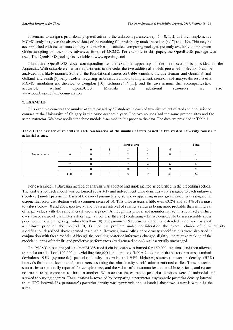
This example concerns the number of tests passed by 52 students in each of two distinct but related actuarial sciencecourses at the University of Calgary in the same academic year. The two courses had the same prerequisites and thesame instructor. We have applied the three models discussed in this paper to the data. The data are provided in Table 1.

Table 1. The number of students in each combination of the number of tests passed in two related university courses inactuarial science.

First course Total0 1 2 3 4

Second course 0 0 0 2 2 0 41 0 0 2 2 1 52 0 0 2 4 6 123 0 0 0 5 26 31

Total 0 0 6 13 33 52

For each model, a Bayesian method of analysis was adopted and implemented as described in the preceding section.The analysis for each model was performed separately and independent prior densities were assigned to each unknown(top-level) model parameter. Each of the model parameters νi, µi, and ω appearing in any given model was assigned anexponential prior distribution with a common mean of 10. This prior assigns a little over 63.2% and 86.4% of its massto values below 10 and 20, respectively, and treats an interval of smaller values as being more probable than an intervalof larger values with the same interval width, a priori. Although this prior is not noninformative, it is relatively diffuseover a large range of parameter values (e.g., values less than 20) containing what we consider to be a reasonable and apriori probable subrange (e.g., values less than 10). The parameter θ appearing in the first extended model was assigneda uniform prior on the interval (0, 1). For the problem under consideration the overall choice of prior densityspecification described above seemed reasonable. However, some other prior density specifications were also tried inconjunction with these models. Although the resulting posterior inferences changed slightly, the relative ranking of themodels in terms of their fits and predictive performances (as discussed below) was essentially unchanged.

The MCMC based analysis in OpenBUGS used 4 chains, each was burned for 150,000 iterations, and then allowedto run for an additional 100,000 thus yielding 400,000 kept iterations. Tables 2 to 4 report the posterior means, standarddeviations, 95% (symmetric) posterior density intervals, and 95% highest (i.e. shortest) posterior density (HPD)intervals for the top-level model parameters assuming the prior density specification mentioned earlier. These posteriorsummaries are primarily reported for completeness, and the values of the summaries in one table (e.g. for ν1 and ν2) arenot meant to be compared to those in another. We note that the estimated posterior densities were all unimodal andskewed to varying degrees. The skewness is revealed by comparing a parameter’s symmetric posterior density intervalto its HPD interval. If a parameter’s posterior density was symmetric and unimodal, these two intervals would be thesame.

32 The Open Statistics & Probability Journal, 2017, Volume 08 David Peter Michael Scollnik

Table 2. Posterior summaries for parameters in the first model.

Parameter Mean Std. Dev. 95% Interval 95% HPD Intervalν1

ν2

ν0

5.7162.7280.707

2.5261.2010.295

(2.383, 11.98)(1.175, 5.683)(0.323, 1.433)

(1.843, 10.75)(0.937, 5.105)(0.259, 1.291)

Table 3. Posterior summaries for parameters in the second model.

Parameter Mean Std. Dev. 95% Interval 95% HPD Intervalν1

ν2

ν0

θ

5.8792.9190.7190.862

3.0731.4770.37030.140

(2.239, 13.52)(1.208, 6.617)(0.289, 1.625)(0.471, 0.997)

(1.695, 11.61)(0.939, 5.66)(0.221, 1.39)(0.572, 1.00)

Table 4. Posterior summaries for parameters in the third model.

Parameter Mean Std. Dev. 95% Interval 95% HPD Intervalµ1

µ2

ν1

ν2

ω

8.5943.9770.3040.2570.810

5.3502.2470.6060.3400.430

(2.876, 23.18)(1.455, 9.722)(0.017, 2.020)(0.035, 1.146)(0.274, 1.907)

(2.07, 20.79)(0.988, 8.756)(0.011, 1.644)(0.0165, 0.925)(0.163, 1.722)

Recall that the data set contains 52 observations. As part of the MCMC based analysis, a predictive replicatedsample of size 52 was generated from the model at each iteration. Summaries of these predictive replicated samples arereported in Tables 5 to 7. Specifically, these tables report the estimated predicted expected value and standard deviationof the number of students (assuming a cohort size of 52 students) in each combination of the number of tests passed inthe two related actuarial science courses, under each model. One may observe that each model’s predicted row andcolumn totals are (for the most part) generally in agreement with those for the original data in Table 1.

Table 5. The predicted expected value (and standard deviation) of the number of students in eachcombination of the number of tests passed in the two related courses under a Bayesian analysis using the firstmodel.

Table 6. The predicted expected value (and standard deviation) of the number of students in eachcombination of the number of tests passed in the two related courses under a Bayesian analysis using the secondmodel.

First course

0 1 2 3 4 Total

0 0.21 (0.49) 0.45 (0.70) 0.75 (0.90) 1.09 (1.10) 1.32 (1.31) 3.82 (2.42)

Second 1 0.18 (0.44) 0.47 (0.70) 0.94 (0.98) 1.66 (1.32) 2.48 (1.66) 5.74 (2.48)

course 2 0.15 (0.40) 0.44 (0.68) 1.07 (1.07) 2.48 (1.66) 5.68 (2.54) 9.82 (3.37)

3 0.09 (0.31) 0.31 (0.57) 0.96 (1.03) 3.44 (2.00) 27.83 (4.94) 32.62 (4.6)

Total 0.64 (0.91) 1.66 (1.41) 3.73 (2.03) 8.67 (3.15) 37.30 (4.13) 52

First course

0 1 2 3 4 Total

0 0.05 (0.23) 0.18 (0.44) 0.40 (0.66) 0.68 (0.87) 0.84 (1.02) 2.14 (1.77)

Second 1 0.08 (0.29) 0.33 (0.59) 0.89 (0.97) 1.88 (1.42) 2.97 (1.87) 6.14 (2.67)

course 2 0.08 (0.29) 0.39 (0.65) 1.33 (1.20) 3.66 (2.01) 8.51 (3.01) 13.97 (3.73)

3 0.05 (0.23) 0.28 (0.56) 1.23 (1.18) 4.84 (2.36) 23.34 (5.05) 29.75 (4.84)

Total 0.26 (0.56) 1.18 (1.22) 3.85 (2.14) 11.06 (3.49) 35.65 (4.52) 52

Bayesian Inference for Three The Open Statistics & Probability Journal, 2017, Volume 08 33

Table 7. The predicted expected value (and standard deviation) of the number of students in eachcombination of the number of tests passed in the two related courses under a Bayesian analysis using the thirdmodel.

Table 8 summarizes the means and standard deviations of the number of tests passed in each course, along with thecorrelation between the two. The first rows of numerical values in this table are the empirical values associated with theobserved data. These are followed by the Bayesian predictive values associated with the three models underconsideration. In this example, it appears that while all three models generally replicate the empirical means andstandard deviations, the first model does a much better job at replicating the correlation than either the second or third.

Table 8. The means and standard deviations of the number of tests passed in each of the two courses, along with thecorrelation between the two courses. The first line gives the observed values corresponding to Table 1; the estimatedpredictive values associated with the first, second, and third models follow.

First course Second course CorrelationMean Std. Dev. Mean Std. Dev.

Observed 3.519 0.699 2.346 0.947 0.667First model 3.545 0.855 2.370 0.946 0.412

Second model 3.551 0.769 2.371 0.847 0.284Third model 3.533 0.752 2.355 0.843 0.246

When the goal is to pick a model with the best out-of-sample predictive power then selection can be made on thebasis of the deviance information criterion (DIC), which is a combined measure of goodness of fit and modelcomplexity. The DIC and its calculation are discussed in Spiegelhalter et al. [12]. See also Chapter 7 in Gelman et al.[11]. The DIC is implemented in OpenBUGS and according to the OpenBUGS User Manual, “the model with thesmallest DIC is estimated to be the model that would best predict a replicate dataset of the same structure as thatcurrently observed”. The values of the DIC corresponding to the models represented in Tables 5 to 7 are 162.9, 164.7,and 169.1, respectively. So based on this criterion, the first of the three models under consideration is the preferredmodel.

Although the DIC is conveniently incorporated in OpenBUGS, it is not without its problems. For instance, it canproduce negative estimates of the effective number of parameters in its evaluation of a model’s complexity and it is notdefined for singular models. See Celeux et al. [13], Gelman et al. [14], Plummer [15], and Spiegelhalter et al. [16]. TheWAIC (Watanabe- Akaike or widely applicable information criterion; Watanabe [17]) is another measure of a model’spredictive accuracy. This criterion is fully Bayesian and works for singular models and may be viewed as animprovement on the DIC (however, the WAIC is not without its own difficulties; see Gelman et al. [14]).Unfortunately, the WAIC is not directly calculated by OpenBUGS, but it is not too difficult to evaluate it using outputfrom OpenBUGS. We did so, using the definition for the version of WAIC found in Gelman et al. [14] The values ofthe WAIC corresponding to the models represented in Tables 5 to 7 are 173.5, 177.4, and 185.7, respectively.Therefore, of the models under consideration, the first again exhibits the best predictive accuracy for the data in Table 1, this time according to the WAIC. We note that other predictive information criteria for Bayesian models doexist, several of which are reviewed by Gelman et al. [14].

Another approach to checking model fit involves focusing attention on a particular test quantity or discrepancymeasure of interest. This test quantity may be a function of the known and unknown parameters as well as of the data.Let such a test quantity be denoted as T (D, φ), with D denoting the data and φ the model parameters. If D pred denotes apredicted replicated data set generated from the model, then the predictive Bayesian p-value is defined as

First course

0 1 2 3 4 Total

0 0.03 (0.18) 0.12 (0.37) 0.33 (0.60) 0.65 (0.86) 0.89 (1.06) 2.03 (1.73)

Second 1 0.05 (0.23) 0.26 (0.53) 0.84 (0.95) 1.99 (1.46) 3.29 (1.96) 6.44 (2.74)

course 2 0.06 (0.25) 0.35 (0.61) 1.36 (1.22) 4.02 (2.10) 8.80 (3.07) 14.59 (3.82)

3 0.04 (0.21) 0.31 (0.58) 1.47 (1.31) 5.74 (2.63) 21.38 (4.95) 28.94 (4.86)

Total 0.18 (0.46) 1.05 (1.14) 4.00 (2.20) 12.41 (3.68) 34.36 (4.64) 52

34 The Open Statistics & Probability Journal, 2017, Volume 08 David Peter Michael Scollnik

(5.20)

where the probability is taken over the posterior distribution of φ and the posterior predictive distribution of D pred.Extreme values of T (D pred, φ) relative to T (D, φ) are evidence of discrepancy between the model and the data. Thus, aBayesian p-value near 0 or 1 provides evidence of model discrepancy. See Gelman et al. [11] for a more detaileddiscussion of Bayesian p-values.

In the present context of an example involving correlated bivariate data, a sensible and meaningful discrepancymeasure is the sample correlation. In the original data set, the sample correlation r = T (D, φ) is equal to 0.667. Recall,as part of our MCMC based analysis, a predictive replicated sample of size 52 was generated from the model understudy at each iteration. For each model, we monitored the posterior predictive distribution of the sample correlation forthe replicated data, i.e. r pred = T (D pred, φ), and monitored its relation to the sample correlation of the original data. Theresults are presented in Table 9, and lend further support to the conclusion that the first of the three models underconsideration is a better fit to the data than either of the two extended models.

Table 9. Posterior predictive summaries for the sample correlation coefficient r pred for the replicated data associated witheach of the two-dimensional beta binomial models.

Model Mean Std. Dev. 95% Interval Bayesian p-valueFirst model 0.412 0.152 (0.097, 0.688) 0.037

Second model 0.284 0.163 (−0.043, 0.589) 0.005Third model 0.246 0.159 (−0.070, 0.547) 0.002

One final check of predictive model performance was performed. For each predictive replicated sample, the sum ofsquared deviations between the predicted and observed cell counts was calculated over the original non-empty cells.Denote this statistic as SS pred. When comparing models, smaller values of this statistic are indicative of a better fit. Theestimated posterior predictive summaries for SS pred are reported in Table 10. Once again, the first of the three modelsunder consideration comes out on top.

Table 10. Posterior predictive summaries for SS pred for the replicated data asso- ciated with each of the two-dimensional betabinomial models.

Model Mean Std. Dev. 95% IntervalFirst model

Second modelThird model

61.1176.5696.1

43.9258.8973.03

(15, 182)(17, 238)(19, 291)

CONCLUSION

This paper considered three two-dimensional beta binomial models. Two of these models do not have closed formsof probability mass functions and are not amenable to analysis using maximum likelihood. Instead, a Bayesian analysisof each model was implemented using MCMC with data augmentation.

In the example contained within this paper, the first of the two-dimensional beta binomial models was the bestperforming model of the three considered. Of course, this does not necessarily mean that it will always perform betterthan the other two. However, as yet we have not run across an actual data set for which the first model did not performat least as well as one of the others.

APPENDIX

This BUGS code can be used with OpenBUGS to implement a Bayesian analysis of the two- dimensional beta binomialmodel presented in Bibby and Væth [4]. The manner of variable indexing and data formatting used in this code is suchthat tables containing cells with zero counts may be conveniently analysed. Only cells with non-zero counts are read inas data.

Pr(T (D pred, φ) ≥ T (D,φ) |D ) ,

Bayesian Inference for Three The Open Statistics & Probability Journal, 2017, Volume 08 35

model{

# Define the model including the prior.

for( cell in 1:cells ) {

for( k in 1:N[cell,3] ) {

for( l in 1:2 ) {

x[cell,k,l] <- N[cell,l] - 1

x[cell,k,l] ~ dbin(p[cell,k,l],n[l])

p[cell,k,l] <- w[cell,k,l] / (w[cell,k,l] + w[cell,k,3])

}

for( l in 1:3 ) {

w[cell,k,l] ~ dchisqr(df.w[l])

}

}

}

for( l in 1:3 ) {

df.w[l] <- 2 * nu.w[l]

nu.w[l] ~ dexp(0.1)

}

# Replicated sample for posterior predictive inference.

for( rep in 1:nobs ) {

for( k in 1:2 ) {

xp[rep,k] ~ dbin(pp[rep,k],n[k])

pp[rep,k] <- wp[rep,k] / (wp[rep,k] + wp[rep,3])

}

for( l in 1:3 ) {

wp[rep,l] ~ dchisqr(nu.w[l])

}

}

for( i in 1:n[1] + 1 ) {

36 The Open Statistics & Probability Journal, 2017, Volume 08 David Peter Michael Scollnik

for( j in 1:n[2] + 1 ) {

for( rep in 1:nobs ) {

np[rep,i,j] <- equals(i,xp[rep,1] + 1) * equals(j,xp[rep,2] + 1)

}

nc[i,j] <- sum(np[1:nobs,i,j])

}

}

for( i in 1:n[1] + 1 ) {

col[i] <- sum(nc[i,1:n[2] + 1])

}

for( j in 1:n[2] + 1 ) {

row[j] <- sum(nc[1:n[1] + 1,j])

}

# Posterior predictive model check.

r.obs <- 0.6672033

r.pred <- ( inprod( xp[,1],xp[,2] ) -

nobs * mean( xp[,1] ) * mean( xp[,2] ) ) /

( ( nobs - 1 ) * sd( xp[,1] ) * sd( xp[,2] ) )

post.pred <- step( r.pred - r.obs )

# Another posterior predictive model check statistic.

for( cell in 1:cells ) {

nc2[cell] <- pow(N[cell,3] - ncsub[cell],2)

ncsub[cell] <- nc[N[cell,1],N[cell,2]]

}

# nc2[cells + 1] is referred to as SS.pred in the main body of the paper.

nc2[cells + 1] <- sum(nc2[1:cells])

ncsub[cells + 1] <- sum(ncsub[1:cells])

Bayesian Inference for Three The Open Statistics & Probability Journal, 2017, Volume 08 37

CONSENT FOR PUBLICATION

Not applicable.

CONFLICT OF INTEREST

The author declares no conflict of interest, financial or otherwise.

ACKNOWLEDGEMENTS

This research was supported by a Discovery Grant from the Natural Sciences and Engineering Research Council ofCanada (NSERC).

REFERENCES

[1] N.L. Johnson, A.W. Kemp, and S. Kotz, Univariate Discrete Distributions., 3rd ed John Wiley & Sons Inc.: New York, 2005.[http://dx.doi.org/10.1002/0471715816]

[2] J.G. Skellam, "A probability distribution derived from the binomial distribution by regarding the probability of success as variable betweenthe sets of trials", J. R. Stat. Soc. B, vol. 10, pp. 257-261, 1948.

[3] G. Ishii, and R. Hayakawa, "On the compound binomial distribution", Annals of the Institute of Statistical Mathematics, Tokyo, vol. 12, pp.

nc2[cells + 2] <- nc2[cells + 1] + pow(nobs - ncsub[cells + 1],2)

}

list( cells = 10, n = c(4,3), nobs = 52, N=structure(

.Data = c(

3, 1, 2,

4, 1, 2,

3, 2, 2,

4, 2, 2,

5, 2, 1,

3, 3, 2,

4, 3, 4,

5, 3, 6,

4, 4, 5,

5, 4, 26

),

.Dim=c(10,3)

)

)

38 The Open Statistics & Probability Journal, 2017, Volume 08 David Peter Michael Scollnik

69-80, 1960.[http://dx.doi.org/10.1007/BF01577666]

[4] B.M. Bibby, and M. Væth, "The two-dimensional beta binomial distribution", Stat. Probab. Lett., vol. 81, pp. 884-891, 2011.[http://dx.doi.org/10.1016/j.spl.2010.12.019]

[5] P.J. Danaher, and B.G. Hardie, "Bacon with your eggs? Applications of a new bivariate beta-binomial distribution", Am. Stat., vol. 59, no. 4,pp. 282-286, 2005.[http://dx.doi.org/10.1198/000313005X70939]

[6] M. Jones, "Multivariate t and beta distributions associated with the multivariate t dis- tribution", Metrika, vol. 54, pp. 215-231, 2001.[http://dx.doi.org/10.1007/s184-002-8365-4]

[7] W.N. Bailey, "Generalized Hypergeometric Series", In: Cambridge Tracts in Mathematics and Mathematical Physics, vol. 32. CambridgeUniversity Press, 1935.

[8] S. Geman, and D. Geman, "Stochastic relaxation, gibbs distributions, and the bayesian restoration of images", IEEE Trans. Pattern Anal.Mach. Intell., vol. 6, no. 6, pp. 721-741, 1984.[http://dx.doi.org/10.1109/TPAMI.1984.4767596] [PMID: 22499653]

[9] A.E. Gelfand, and A.F. Smith, "Sampling-based approaches to calculating marginal densities", J. Am. Stat. Assoc., vol. 85, no. 410, pp.398-409, 1990.[http://dx.doi.org/10.1080/01621459.1990.10476213]

[10] P. Congdon, Bayesian Statistical Modelling., 2nd ed John Wiley & Sons Ltd: West Sussex, 2006.[http://dx.doi.org/10.1002/9780470035948]

[11] A. Gelman, J.B. Carlin, H.S. Stern, D.B. Dunson, A. Vehtari, D.B. Rubin, Bayesian Data Analysis., 3rd ed Chapman & Hall / CRC: NewYork, 2014.

[12] D.J. Spiegelhalter, N.G. Best, B.P. Carlin, and A. van der Linde, "Bayesian measures of model complexity and fit (with discussion)", J. R.Stat. Soc. B, vol. 64, pp. 583-640, 2002.[http://dx.doi.org/10.1111/1467-9868.00353]

[13] G. Celeux, F. Forbes, C. Robert, and D. Titterington, "Deviance information criteria for missing data models", Bayesian Anal., vol. 1, pp.651-706, 2006.[http://dx.doi.org/10.1214/06-BA122]

[14] A. Gelman, J. Hwang, and A. Vehtari, "Understanding predictive information criteria for Bayesian models", Stat. Comput., vol. 24, pp.997-1016, 2014.[http://dx.doi.org/10.1007/s11222-013-9416-2]

[15] M. Plummer, "Penalized loss functions for Bayesian model comparison", Biostatistics, vol. 9, no. 3, pp. 523-539, 2008.[http://dx.doi.org/10.1093/biostatistics/kxm049] [PMID: 18209015]

[16] D.J. Spiegelhalter, N.G. Best, B.P. Carlin, and A. van der Linde, "The deviance information criterion: 12 years on", J. R. Stat. Soc. B, vol. 76,pp. 485-493, 2014.[http://dx.doi.org/10.1111/rssb.12062]

[17] S. Watanabe, "Asymptotic equivalence of Bayes cross validation and widely applicable information criterion in singular learning theory", J.Mach. Learn. Res., vol. 11, pp. 3571-3591, 2010.

© 2017 David Peter Michael Scollnik.

This is an open access article distributed under the terms of the Creative Commons Attribution 4.0 International Public License (CC-BY 4.0), acopy of which is available at: https://creativecommons.org/licenses/by/4.0/legalcode. This license permits unrestricted use, distribution, andreproduction in any medium, provided the original author and source are credited.