The Online Journal of Science and Technology · The Online Journal of Science and Technology - October 2016Volume 6, Issue 4 ... 2Technical University of Liberec, Institute for Nanomaterials,

The Online Journal of Science and Technology

Prof. Dr. Aytekin İşman Editor‐in‐Chief

Prof. Dr. Mustafa Şahin Dündar Editor

Hüseyin Eski Technical Editor

www.tojsat.net October 2016

ISSN 2146‐7390

Copyright © 2016 ‐ THE ONLINE JOURNAL OF SCIENCE AND TECHNOLOGY

All rights reserved. No part of TOJSAT’s articles may be reproduced or utilized in any form or by any means, electronic or mechanical, including photocopying, recording, or by any information storage and retrieval system, without permission in writing from the publisher. Published in TURKEY

Contact Address:

Prof. Dr. Mustafa Şahin Dündar ‐ TOJSAT, Editor Sakarya‐Turkey

The Online Journal of Science and Technology - October 2016 Volume 6, Issue 4

www.tojsat.net Copyright © The Online Journal of Science and Technology

Message from the Editor-in-Chief

Dear Colleagues, TOJSAT welcomes you. TOJSAT would like to thank you for your online journal interest. The online journal system has been diffused very fast for last ten years. We are delighted that a lot of academicians from around the world have visited TOJSAT. It means that TOJSAT has continued to diffuse new trends in science and technology to all over the world since January, 2011. We hope that the volume 6, issue 4 will also successfully accomplish our global science and technology goal. TOJSAT is confident that readers will learn and get different aspects on science and technology. Any views expressed in this publication are the views of the authors and are not the views of the Editor and TOJSAT. TOJSAT thanks and appreciate the editorial board who have acted as reviewers for one or more submissions of this issue for their valuable contributions. TOJSAT will organize ISTEC-2016- International Science & Technology Conference (www.iste-c.net) between July 17-19, 2017 in Berlin, Germany. This conference is now a well-known science and technology event. It promotes the development and dissemination of theoretical knowledge, conceptual research, and professional knowledge through conference activities. Its focus is to create and disseminate knowledge about science and technology. ISTEC-conference books have been published at http://www.iste-c.net/istecpubs For any suggestions and comments on the international online journal TOJSAT, please do not hesitate to fill out the comments & suggestion form. Call for Papers TOJSAT invites you article contributions. Submitted articles should be about all aspects of science and technology. The articles should be original, unpublished, and not in consideration for publication elsewhere at the time of submission to TOJSAT. Manuscripts must be submitted in English. TOJSAT is guided by it’s editors, guest editors and advisory boards. If you are interested in contributing to TOJSAT as an author, guest editor or reviewer, please send your cv to editor. October 01, 2016 Prof. Dr. Aytekin ISMAN Editor-in-Chief Sakarya University



Message from the Editor

Dear Tojsat Readers,

Today, we have reached to the end of sixth volume of our journal. With the sixth volume six years past from the journals’ first issue published on-line. Our goal is to rewiev and accept multi disciplinary research papers, rewiev articles, etc. for the journal from scientific World such as “Computational Design Optimization of Road Speed Bump”, “Adsorption Characteristics of Surfactants on Different Petroleum Reservoir Materials” in this issue of journal.

I will thank to the readers all around the World for supports by sending their valuable scientific studies to publish in Tojsat journal.

Prof. Dr. M. Şahin DÜNDAR

Editor



Editor‐in‐Chief

Prof. Dr. Aytekin İŞMAN ‐ Sakarya University, Turkey

Editor

Prof. Dr. Mustafa Şahin DÜNDAR ‐ Sakarya University, Turkey

Technical Editor

Hüseyin Eski, Sakarya University, Turkey

Editorial Board

Prof. Dr. Ahmet APAY,Sakarya University,Turkey

Prof. Dr. Antoinette J. MUNTJEWERFF,University of Amsterdam,Netherlands

Prof. Dr. Arvind SINGHAL,University of Texas,United States

Prof. Dr. Aytekin İŞMAN,Sakarya University,Turkey

Prof. Dr. Bilal GÜNEŞ,Gazi University,Turkey

Prof. Dr. Brent G. WILSON,University of Colorado at Denver,United States

Prof. Dr. Cafer ÇELİK,Ataturk University,Turkey

Prof. Dr. Chih‐Kai CHANG,National University of Taiwan,Taiwan

Prof. Dr. Chin‐Min HSIUNG,National Pingtung University,Taiwan

Prof. Dr. Colin LATCHEM,Open Learning Consultant,Australia

Prof. Dr. Deborah E. BORDELON,Governors State University,United States

Prof. Dr. Don M. FLOURNOY,Ohio University,United States

Prof. Dr. Feng‐Chiao CHUNG,National Pingtung University,Taiwan

Prof. Dr. Finland CHENG,National Pingtung University,Taiwan

Prof. Dr. Francine Shuchat SHAW,New York University,United States

Prof. Dr. Frank S.C. TSENG,National Kaohsiung First University os Science and Technology,Taiwan

Prof. Dr. Gianni Viardo VERCELLI ,University of Genova,Italy

Prof. Dr. Gilbert Mbotho MASITSA,Universirty of The Free State,South Africa

Prof. Dr. Gregory ALEXANDER,University of The Free State,South Africa

Prof. Dr. Gwo‐Dong CHEN,National Central University Chung‐Li,Taiwan

Prof. Dr. Gwo‐Jen HWANG,National Taiwan University od Science and Technology,Taiwan

Prof. Dr. Hellmuth STACHEL,Vienna University of Technology,Austria

Prof. Dr. J. Ana DONALDSON,AECT Former President,United States

Prof. Dr. Mehmet Ali YALÇIN,Sakarya University,Turkey

Prof. Dr. Mustafa S. DUNDAR,Sakarya University,Turkey

Prof. Dr. Nabi Bux JUMANI,International Islamic University,Pakistan

Prof. Dr. Orhan TORKUL,Sakarya University,Turkey

Prof. Dr. Paolo Di Sia,University of Verona,Italy

Prof. Dr. Ümit KOCABIÇAK,Sakarya University,Turkey

Assist. Prof. Dr. Engin CAN,Sakarya University,Turkey

Assist. Prof. Dr. Hüseyin Ozan Tekin,Üsküdar University,Turkey

Assist. Prof. Dr. Tuncer KORUVATAN,Turkish Military Academy,Turkey

Dr. Abdul Mutalib LEMAN,Universiti Tun Hussein Onn Malaysia,Malaysia

Dr. Abdülkadir MASKAN,Dicle University,Turkey

Dr. Alper Tolga KUMTEPE,Anadolu University,Turkey



Dr. Atilla YILMAZ,Hacettepe University,Turkey

Dr. Bekir SALIH,Hacettepe University,Turkey

Dr. Berrin ÖZCELİK,Gazi University,Turkey

Dr. Burhan TURKSEN,TOBB University of Economics and Technology,Turkey

Dr. Chua Yan PIAW,University of Malaya,Malaysia

Dr. Constantino Mendes REI,Instituto Politecnico da Guarda,Portugal

Dr. Daniel KIM,The State University of New York,South Korea

Dr. Dong‐Hoon OH,Universiy of Seoul,South Korea

Dr. Evrim GENÇ KUMTEPE,Anadolu University,Turkey

Dr. Fabricio M. DE ALMEIDA

Dr. Fahad N. ALFAHAD,King Saud University,Saudi Arabia

Dr. Fatimah HASHIM,Universiti Malaya,Malaysia

Dr. Fatma AYAZ,Gazi University,Turkey

Dr. Fonk SOON FOOK,Universiti Sains Malaysia,Malaysia

Dr. Galip AKAYDIN,Hacettepe University,Turkey

Dr. Hasan MUJAJ,University of Prishtina,Kosovo

Dr. Hasan KIRMIZIBEKMEZ,Yeditepe University,Turkey

Dr. Hasan OKUYUCU,Gazi University,Turkey

Dr. Ho Sooon MIN,INTI International University,Malaysia

Dr. Ho‐Joon CHOI,Kyonggi University,South Korea

Dr. HyoJin KOO,Woosuk University,South Korea

Dr. Jae‐Eun LEE,Kyonggi University,South Korea

Dr. Jaroslav Vesely,BRNO UNIVERSITY OF TECHNOLOGY,Czech Republic

Dr. Jon Chao HONG,National Taiwan Normal University,Taiwan

Dr. Joseph S. LEE,National Central University,Taiwan

Dr. Kendra A. WEBER,University of Minnesota,United States

Dr. Kim Sun HEE,Woosuk University,South Korea

Dr. Latif KURT,Ankara University,Turkey

Dr. Li YING,China Central Radio and TV University,China

Dr. Man‐Ki MOON,Chung‐Ang University,South Korea

Dr. Martha PILAR MéNDEZ BAUTISTA,EAN University, Bogotá,Colombia

Dr. Md Nor Noorsuhada,Universiti Teknologi MARA Pulau Pinang,Malaysia

Dr. Mohamad BIN BILAL ALI,Universiti Teknologi Malaysia,Malaysia

Dr. Mohamed BOUOUDINA,University of Bahrain,Bahrain

Dr. Mohammad Reza NAGHAVI,University of Tehran,Iran

Dr. Mohd Roslan MODH NOR,University of Malaya,Malaysia

Dr. Muhammed JAVED,Islamia University of Bahawalpur,Pakistan

Dr. Murat DİKER,Hacettepe University,Turkey

Dr. Mustafa KALKAN,Dokuz Eylül Universiy,Turkey

Dr. Nihat AYCAN,Muğla University,Turkey

Dr. Nilgün TOSUN,Trakya University,Turkey

Dr. Nursen SUCSUZ,Trakya University,Turkey

Dr. Osman ANKET,Gülhane Askeri Tıp Akademisi,Turkey

Dr. Piotr TOMSKI,Czestochowa University of Technology,Poland

Dr. Raja Rizwan HUSSAIN,King Saud University,Saudi Arabia

Dr. Ramdane YOUNSI,Polytechnic University,Canada

Dr. Rıdvan KARAPINAR,Yuzuncu Yıl University,Turkey

Dr. Rıfat EFE,Dicle University,Turkey

Dr. Ruzman Md. NOOR,Universiti Malaya,Malaysia

Dr. Sandeep KUMAR,Suny Downstate Medical Center,United States

Dr. Sanjeev Kumar SRIVASTAVA,Mitchell Cancer Institute,United States

Dr. Selahattin GÖNEN,Dicle University,Turkey

Dr. Senay CETINUS,Cumhuriyet University,Turkey

Dr. Sharifah Norul AKMAR,University of Malaya,,Malaysia

Dr. Sheng QUEN YU,Beijing Normal University,China

Dr. Sun Young PARK,Konkuk University,South Korea

Dr. Tery L. ALLISON,Governors State University,United States



Dr. Türkay DERELİ,Gaziantep University,Turkey

Dr. Uner KAYABAS,Inonu University,Turkey

Dr. Wan Mohd Hirwani WAN HUSSAIN,Universiti Kebangsaan Malaysia,Malaysia

Dr. Wan Zah WAN ALI,Universiti Putra Malaysia,Malaysia

Dr. Yueah Miao CHEN,National Chung Cheng University,Taiwan

Dr. Yusup HASHIM,Asia University,Malaysia

Dr. Zawawi ISMAIL,University of Malaya,Malaysia

Dr. Zekai SEN,Istanbul Technical University,Turkey



Table of Contents

A COMPARISON OF CURVE INTERPOLATION ALGORITHMS FOR LOW CURVATURE CURVES 1

Vojtech Wrnata, Petr Kretschmer

ADSORPTION CHARACTERISTICS OF SURFACTANTS ON DIFFERENT PETROLUEM RESERVOIR MATERIALS 6

Samya D. Elias, Ademola M. Rabiu, Oyekola Oluwaseun, Beverly Seima

AN APPLICATION FOR THE DEVELOPMENT OF PROCESS CONTROL TRAINING SET 17

Aydın GÜLLÜ, Hilmi KUŞÇU, M. Ozan AKI

ASSESMENT OF THE USE OF DIATOMITE AND PUMICE IN STONE MASTIC ASPHALT AS STABILIZER 22

Bekir AKTAŞ, Şevket ASLAN

AUTOMATIC GENERATION OF CONFUSABLE SETS IN SMART SPELL CHECKING FOR KOREAN LEARNERS OF ENGLISH

26

Kong Joo Lee, Jee Eun Kim

CLASSIFYING HAND SIGNS USING IMAGE PROCESSING 32

Ozan AKI, Aydın GÜLLÜ

COMPUTATIONAL DESIGN OPTIMIZATION OF ROAD SPEED BUMPS 36

Hakan ERSOY, Kayra KURŞUN

FINITE ELEMENT SOLUTION OF DIM DAM UNDER STATIC LOADING USING DUNCAN CHANG MODELLING 42

Ergin ERAYMAN, Mustafa YILDIZ, Uğur Ş. ÇAVUŞ, Ali YILDIZ

TIME‐DEPENDENT CHANGE OF SEISMIC VELOCITIES ON LOWSTRENGTH CONCRETE 49

Nevbahar SABBAĞ, Osman UYANIK

WAVELENGTH DIVISION MULTIPLEXING AND ENERGY EFFICIENCY 58

Öznur ŞENGEL, Muhammed Ali AYDIN



A COMPARISON OF CURVE INTERPOLATION ALGORITHMS FOR LOW CURVATURE CURVES

Vojtech Wrnata1, Petr Kretschmer2

1Technical University of Liberec, Faculty of Mechatronics, Informatics and Interdisciplinary Studies, Studentska 1402/2, 461 17, Liberec, Czech Republic

[email protected]

2Technical University of Liberec, Institute for Nanomaterials, Advanced Technology and Innovation, Studentska 1402/2, 461 17, Liberec, Czech Republic

[email protected]

Abstract:This paper presents a comparison of two algorithms for low curvature curves. The two compared algorithms are: linear interpolation and interpolation with Bézier curves. The comparison of the interpolation accuracy is verified on a calculation of the length of the reference curve with different curvature and degree of discretization. Arcs of a circle are used as reference curves. The comparison of the accuracy of the length of an interpolled curve and arc shows that interpolation with Bézier curves is always more accurate regardless the curve curvature.

Keywords: Algorithm, Arc length, Bézier, Curves, Interpolation

Introduction When modelling nanofiber or microfilament structures an image analysis is used to acquire the geometry of fibre layers. Single fibres are represented by points, which the fibres intersect. These points are then interpolled with curves. An observation of real structures points at the fact that fibres in a structure are laid so that they create curves with low curvature. This paper aims to compare two interpolation algorithms - linear interpolation and interpolation with Bézier curves - in order to find out which algorithm is more accurate for fibre interpolation. The accuracy of the algorithms is verified on a calculation of the length of reference curves with different curvature and discretization.

REFERENCE CURVES CURVE CURVATURE Curve curvature C was defined as the ratio of height H and length L, C = H/L, see Fig. 1. The curvature in range 0.2-0.02 was chosen for the curves tested in the article. The range reflects the real material fibres in fibre layers. Fig. 1 shows a curve with curvature 0.2.


www.tojsat.net Copyright © The Online Journal of Science and Technology 1

Fig. 1. Reference curve with curvature 0.2

REFERENCE CURVES An arc of a circle was chosen as a reference curve. The arc’s curvature was changed in the 0.2-0.02 range. The arc of a circle was chosen due to its easy calculation of its length and easy discretization. The discretization step was chosen in the range 5-20. This range reflects real characteristics of interpolled fibres, i.e. it reflects the way how the interpolled points are obtained from real fibre structures. The arc was chosen so that it always intersects the [0.0, 0.0] and [0.1, 0.0] points. The radius of the circle was calculated so that the centre of the circle was laid on the x coordinate 0.5, y coordinate of the circle centre was calculated for the given curvature of the arc. The length of the curve was calculated from the known coordinate of the circle centre. Table 1 contains data of 10 reference arcs.

Table 1. Reference arcs

Curvature Arc length Centre Angle α 0.02 1.0010663255671826 [0.5, -6.2399] 0.15991474849316017 0.04 1.0042612202599455 [0.5, -3.105] 0.31931994284894927 0.06 1.009572521275021 [0.5, -2.0533] 0.4777157040733537 0.08 1.016980230614833 [0.5, -1.5225] 0.6346210487456057 0.10 1.02645691121938 [0.5, -1.2] 0.789582239399523 0.12 1.0379682150432712 [0.5, -0.9816] 0.9421799228834535 0.14 1.051473519316817 [0.5, -0.8229] 1.0920348123468426 0.16 1.0669266439487615 [0.5, -0.7012] 1.2388117781698247 0.18 1.0842766217363944 [0.5, -0.6044] 1.3822223223268484 0.20 1.103468493625858 [0.5, -0.525] 1.5220255084494594

ARC DISCRETIZATION The interpolation points are acquired by the arc discretization into a required number of parts. The discretization is conducted by an equidistant partition of the angle α, see Fig. 2. The coordinates of points are calculated as an intersection of the reference arc and circle 2 2 2, where r is the distance from the [0.0, 0.0] point to point, see Fig. 2. The distance is calculated from the reference arc parameters. The calculation is based on the discretization into 5-20 parts.



Fig. 2. Arc discretization

INTERPOLATION ALGORITHMS LINEAR INTERPOLATION Linear interpolation joints points by abscissae. The length of the arc is calculated as a sum of the lengths of each part, accordingly to the following pattern:

∑ (1)

where is the number of parts and is the length of - part. The length of the part is calculated accordingly:

(2)

where , are or coordinates of the - part or 1 part of the arc.

INTERPOLATION WITH B-SPLINE CURVES Segments of cubic Bézier curves in connection with were used for the interpolation. A segment from a cubic Bézier curve is created between each two points. Its control points are calculated with the help of so-called "A-frame". The algorithm for calculating the control points is described in detail, for example, in chapter 5 of [1] or [2]. The length of the B-spline curve is calculated accordingly to pattern (1), where is the length of an segment of the B-spline curve. The length of the segment is calculated with the help of linear interpolation with step 20.

Results The results of the algorithms comparison are presented in graphs. The graph in Fig. 3 shows the dependence of relative length deviation ε on the degree of discretization (the number of discretization steps), for the curvature 0.02, 0.1 and 0.2. The graph in Fig. 4 shows the dependence of relative length deviation ε on curve curvature, for discretization 5, 10 and 20. Fig. 5 shows the dependence ration of relative deviations of linear interpolation and B-spline curve interpolation on the degree of discretization (a number of discretization steps), for curve curvature 0.02, 0.1 and 0.2. The ration of relative deviations is defined as:

(3)

where ε is a relative length deviation of linear interpolation and ε relative length deviation of B-

spline curve interpolation. The ration of relative deviations ε is defined accordingly:

ε (4)

where is a calculated length and is a real length.



Fig. 3. The dependence of the relative length deviation ε on the degree of discretization for curvature 0.02, 0.1

and 0.2.

Fig. 4. The dependence of relative length deviation ε on the curve curvature for linear interpolation and B-spline

curve interpolation.



Fig. 5. The dependence ratio of relative length deviations of linear interpolation and B-spline curve interpolation

on the degree of discretization, for curve curvature 0.02, 0.1 and 0.2.

Conclusions The comparison of the algorithms has proved the assumption B-spline curve interpolation is more accurate. The accuracy of the interpolation was verified on ten arcs with curvature from 0.02 to 0.2. The algorithms were verified on all arcs with the discretization range 5-20. The utilization of B-spline curve interpolation was more accurate in all cases.

Acknowledgements The work of Vojtech Wrnata was supported by the Ministry of Education of the Czech Republic within the SGS project no. 21066/115 on the Technical University of Liberec. The work of Petr Kretschmer was obtained through the financial support of the Ministry of Education, Youth and Sports in the framework of the targeted support of the "National Programme for Sustainability I" and the OPR\&DI project Centre for Nanomaterials, Advanced Technologies and Innovation CZ.1.05/2.1.00/01.0005.

References Baker, K.A., The Mathematics of Computer Graphics, Cubic spline curves, Department of Mathematics, UCLA,

Los Angeles, 2002, url = http://www.math.ucla.edu/~baker/149.1.02w/handouts/dd_splines.pdf Sederberg, T.W., Computer aided geometric design, Department of Computer Science, Brigham Young

University, 2014, url = http://tom.cs.byu.edu/~557/text/cagd.pdf



ADSORPTION CHARACTERISTICS OF SURFACTANTS ON DIFFERENT PETROLUEM RESERVOIR MATERIALS

Samya D. Elias, Ademola M. Rabiu, Oyekola Oluwaseun and Beverly Seima

Department of Chemical Engineering, Cape Peninsula University of Technology

Bellville, Cape Town 7535, South Africa [email protected]

Abstract: The loss of injected chemical(s) in the reservoir during injection due to the adsorption of the surfactant (and co-surfactants) unto the rock materials weighs heavily on the economics and environmental footprint of the process and remains a focus of research attention. It is necessary that the surfactant loss in the reservoir during injection is minimized to improve on the process economics and ensure its wider application. In this study the adsorption of cationic and anionic surfactants onto the common reservoir rock material and drilling mud weighing agent is investigated at various surfactant concentration and salinity. The effect of pH was also studied by formulating an alkaline-surfactant mixture using various concentration of NaOH. The indirect method of residual equilibrium surfactant concentration measurement was employed to obtain the adsorption isotherm of cetyltrimethyl-ammonium bromide (CTAB) and sodium dodecyl sulfate (SDS) on kaolin, silica, alumina and ilmenite. Surfactant concentration was varied from 50-600 ppm and the conductivity of the equilibrated media at room temperature is measured at various brine concentration and pH. Both surfactants were found to adsorb strongly onto the rock materials while stabilization in the level of adsorption in the region above the CMC was observed as the monomer concentration falls due to micelles formation. At same level of salinity, it was found that cationic surfactant adsorbed more strongly on the rock materials that the anionic surfactant. The volume adsorbed was found to increase up to a maximum of 1.170 mg/g and 1.8249 mg/g for SDS and CTAB respectively on kaolin and ilmenite for instance, as the concentration was increased at constant salinity. The same trend was noted as the brine concentration was varied with adsorption increasing with salinity for anionic surfactant. As pH increases the volume adsorption for SDS decreases while the opposite was the case with the cationic surfactant, CTAB which increase with the alkalinity of the solution. Keywords:Adsorption, Surfactant, Petrolium Reservoir

Introduction Surfactant flooding is widely employ to manipulate the phase behaviour of the reservoir fluids to counteract the high capillary force trapping oil in the pores of the reservoir during enhanced oil recovery process (Babu et al., 2015;Kamari et al., 2015;Zargartalebi et al., 2015). The surface active chemical promote the formation of microemulsions at the crude oil and the displacing fluid (mostly water) interface (Ahmadi & Shadizadeh, 2015;Spildo et al., 2014) thus causing a significant lowering of the fluids interfacial tension (IFT). This is required to efficiently mobilize a substantial percentage of the residual oil towards the production wells to enhance overall crude recovery (Lu et al., 2014). The major problem that affects the efficiency of tertiary oil recovery during micellar flooding, steam-surfactant flooding, alkaline-surfactant (AS), surfactant-polymer (SP) or alkaline-surfactant-polymer (ASP) is the loss of surfactant through interaction with reservoir rock (Ponce F et al., 2014), along with surfactant partitioning into the oil interface (Bera et al., 2013). In surfactant-water-solid systems, the quantity of surfactant adsorbed depends on the rock properties (surface charge for instance), the character of the surfactant (kind of surfactant, the chain structure), temperature, salinity in addition to the pH (Qiao et al., 2012;Sheng, 2011). Other mechanisms that may cause surfactant losses include precipitation of surfactant when in the presence of electrolyte ions and surfactant diffusion in to dead-end pores (ShamsiJazeyi et al., 2014;Tichelkamp et al., 2015). High adsorption of surfactants onto the reservoir rock causes surfactant chromatographic retardation while they are carried through a reservoir formation, thus turning the EOR project unproductive and economically not viable (Ma et al., 2013). Dynamic and balanced surfactants adsorption at the solid/liquid interface is mainly dependent on the surfactants nature as well as on the nature of the reservoir rock surface



(Hosna Talebian et al., 2015;Romero-Zerón & Kittisrisawai, 2015;Zhang & Somasundaran, 2006). Hence, the choice and selection of surfactant for Chemical Enhanced Oil Recovery (CEOR) operation is influenced by the oil reservoir materials and conditions as well (Kamari et al., 2015). Depending on the rock formation, oil reservoirs are typically categorized into two types: carbonate and sandstone (Dandekar, 2013;Lashkarbolooki et al., 2014). Anionic surfactants are generally preferred in sandstone reservoir formations owing to the fact that they are relatively less adsorbed in comparison to any of nonionics, cationics as well as zwitterionics surfactants (Ma et al., 2013). These reservoirs comprises of huge quantities of quartz (silica) and less of silicate and carbonate rock crystals and the arrangement is dependent on the sedimentology of the reservoir formation. The majority of solid surfaces of reservoir rocks are charged, for instance silica is predominantly negative charge, while calcite, alumina and dolomite are positively charged at neutral pH (Cappelletti et al., 2006;Yoshihara et al., 1996). If the surfactant being injected and the reservoir material (adsorbent) have different charges, the degree of adsorption is very rapid and the time of equilibrium time is reduced (Muherei & Junin, 2009). In contrast, if the surfactant and the reservoir material have the same charge, repulsive interaction occur which results in negligible adsorption (Wesson & Harwell, 2010). Surfactant adsorption has been found to increase as the surface charge of the reservoir rock increases in the direction of the more positive charges (Pei et al., 2014), which is in accordance with the mechanism of electrostatic. Bastrzyk and Sadowski (2012) reported that CTAB exhibited higher adsorption comparing to SDS on both natural dolomite and magnesite in a low-salinity solution consisting of 0.0001 M of sodium chloride. Significant adsorption of cationic surfactants may be expected to occur if the carbonate formation is rich in clay and/or silica (Ma et al., 2013). To fully comprehend the scheme of surfactant adsorption taking place on carbonates and precisely select the right surfactants for CEOR processes in carbonate rock formations, Ma et al. (2013) studied the adsorption of anionic and cationic surfactants using natural and synthetic carbonate materials. They also looked into likely impurities in natural carbonate, for example clay and silica. Sodium dodecyl sulfate (SDS) and cetylpyridinium chloride (CPC) were selected as the cationic and anionic surfactants, correspondingly. CPC showed insignificant adsorption when synthetic calcite was used but then again quite high adsorption on a number of natural carbonates. It was observed that the adsorption plateau of CPC on carbonates was highly dependent on the amount of silica in the carbonate samples as a result of the strong electrostatic interaction among CPC and the negative binding sites in clay and/or silica. Other researchers have studied the effect of pH and salinity on the adsorption of surfactants (Delshad et al., 2013;Dong et al., 2013;Olajire, 2014;Sheng, 2013a; 2013b;Yuan et al., 2015;Zhao et al., 2015). Generally, addition of alkali to raise the pH is able to change the surface charge to alter the adsorption quantity; the salinity may alter the electrical potential of surface sites for the adsorption (Wesson & Harwell, 2010;Yuan et al., 2015). Adding salts of multivalent cations can sometimes cause a significant increase in the adsorption of anionic surfactants but a considerably decrease in the adsorption of cationic surfactants (Salari et al., 2011). In general, the most used technique to determine the surfactant loss through adsorption onto the porous medium during a surfactant core flood, is the method of depletion, where the change in the amount of surfactant after it comes in contact with adsorbents is registered and said to be adsorbed. The results obtained from determining the adsorption experimentally are usually represented as adsorption isotherms, where the quantity of surfactant adsorbed is given as a function of equilibrium concentrations (Bera et al., 2013;Salari et al., 2011;Xiao et al., 2003). Adsorption isotherms are determined by maintaining solution environment states, for instance pH, temperature and ionic strength constant (Touhami et al., 1998). When determining surfactant adsorption in dispersed systems, a known quantity of surfactant is added to the system and allowed to reach equilibrium. Afterwards the dispersed solids are separated and the surfactant concentration in the solution measured (Salari et al., 2011). Surfactant adsorption is given by the relationship:

Γ 10 (1)

where,

is the adsorption density (mg/g), is the initial surfactant concentration (ppm), is the equilibrium surfactant concentration in solution (ppm), is the mass of the surfactant solution (g) and is the mass of the dry absorbents (g). Adsorption models are normally needed to estimate the loading on the adsorption medium at a certain concentration of the element being studied. The two most common adsorption isotherms which are utilized to model the equilibrium



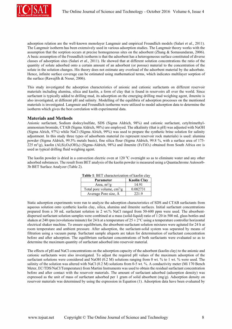
adsorption relation are the well-known monolayer Langmuir and empirical Freundlich models (Salari et al., 2011). The Langmuir isotherm has been extensively used in various adsorption studies. The Langmuir theory works with the assumption that the sorption occurs at precise homogeneous sites on the adsorbent (Zhang & Somasundaran, 2006). A basic assumption of the Freundlich isotherm is that the adsorbent has a heterogeneous surface constituted of diverse classes of adsorption sites (Salari et al., 2011). He showed that at different solution concentrations the ratio of the quantity of solute adsorbed onto a certain amount of an adsorbent (or porous) material to the concentration of the solute in the solution changes. His theory does not estimate any overload of the adsorbent material by the adsorbate. Hence, infinite surface coverage can be estimated using mathematical terms, which indicates multilayer sorption of the surface (Rawajfih & Nsour, 2006). This study investigated the adsorption characteristics of anionic and cationic surfactants on different reservoir materials including alumina, silica and kaolin, a form of clay that is found in reservoirs all over the world. Since surfactant is typically added to drilling mud, its adsorption on the emerging drilling mud weighing agent, ilmenite is also investigated, at different pH and salinity. Modelling of the equilibria of adsorption processes on the mentioned materials is investigated. Langmuir and Freundlich isotherms were utilized to model adsorption data to determine the isotherm which gives the best correlation with experimental data. Materials and Methods Anionic surfactant, Sodium dodecylsulfate, SDS (Sigma Aldrich, 98%) and cationic surfactant, cetyltrimethyl-ammonium bromide, CTAB (Sigma Aldrich, 98%) are employed. The alkalinity (that is pH) was adjusted with NaOH (Sigma Alrich, 97%) while NaCl (Sigma Alrich, 99%) was used to prepare the synthetic brine solution for salinity adjustment. In this study three types of adsorbents material (to represent reservoir rock materials) is used: alumina powder (Sigma Aldrich, 99.5% metals basis), fine silica flour (Sigma Aldrich, 99.8 %, with a surface area of 175-225 m2/g), kaolin (Al2Si2O5(OH)4) (Sigma-Aldrich, 98%) and ilmenite (FeTiO3) obtained from South Africa ore is used as typical drilling fluid weighing agent. The kaolin powder is dried in a convection electric oven at 120 0C overnight so as to eliminate water and any other adsorbed substances. The result from BET analysis of the kaolin powder is measured using a Quantachrome Autosorb-3b BET Surface Analyzer (Table 2).

Table 1: BET characterization of kaolin clay Parameter Kaolin Clay Area, m2/g 14.91

Total pore volume, cm3/g 0.082731 Average Pore size, Å 221.9

Static adsorption experiments were run to analyze the adsorption characteristics of SDS and CTAB surfactants from aqueous solution onto synthetic kaolin clay, silica, alumina and ilmenite surfaces. Initial surfactant concentrations prepared from a 30 mL surfactant solution in 2 wt.% NaCl ranged from 50-600 ppm were used. The absorbent-dispersed surfactant solution samples were combined at a mass (solid-liquid) ratio of 1:20 in 500 mL glass bottles and shaken at 240 rpm (revolutions/minute) for 24 h at a temperature of 25 ± 2°C using a temperature controller horizontal electrical shaker machine. To ensure equilibrium, the absorbent-surfactant solution mixtures were agitated for 24 h at room temperature and ambient pressure. After adsorption, the surfactant-solid system was separated by means of filtration using a vacuum pump. Surfactant sample aliquots are taken for determination of surfactant concentration before and after adsorption. The equilibrium surfactant concentrations of both surfactants were evaluated so as to determine the maximum quantity of surfactant adsorbed into reservoir material. The effects of pH and NaCl concentrations on the adsorption capacity of the adsorbent (kaolin clay) to the anionic and cationic surfactants were also investigated. To adjust the required pH values of the maximum adsorption of the surfactant solutions were considered and NaOH (0.2 M) solutions ranging from 0 wt. % to 1 wt. % were used. The salinity of the solution was altered with NaCl (0.2 M) solutions from 0-5 wt. %. A conductivity meter (Mi 170 Bench Meter, EC/TDS/NaCl/Temperature) from Martini Instruments was used to obtain the residual surfactant concentration before and after contact with the reservoir materials. The amount of surfactant adsorbed (adsorption density) was expressed as the unit of mass of surfactant adsorbed per 1 gram of solid absorbent (mg/g). Adsorption density on reservoir materials was determined by using the expression in Equation (1). Adsorption data have been evaluated by



fitting with Langmuir and Freundlich isotherm models. Findings In Figures 1 and through 4 illustrates the adsorption isotherm for SDS and CTAB on the representative reservoir rock materials, that is, synthetic kaolin powder, alumina and silica and the weighing agent, ilmenite at ambient temperature and constant pH of 6.0. The solution salinity was kept constant with 2 vol % NaCl solution. It could be seen from the Figure 1 that both the anionic and cationic surfactant exhibit significant adsorption unto the kaolin clay. This is due to the presence of both negative and positive binding sites happen on this mineral surface at the prevailing pH. This was reported to be the case in other published works (for instance, (Xu et al., 1991), Zhou and Gunter (1992), Jiang et al. (2010), Ma et al. (2013)). The same happened when ilmenite was used (see Figure 2) as its surface is net negatively charged. With an increase in surfactant concentration, it could be seen that SDS adsorption density increased from 0.3960 mg/g at 50 ppm to 1.170 mg/g at surfactant concentration of 250 ppm when kaolin clay was used. On ilmenite however, a very small increase in the adsorption of SDS is observed from 0.27 mg/g to 0.99 mg/g over 50 to 300 ppm.

Figure 1: Static adsorption on Kaolin clay Figure 2: Static adsorption on Ilmenite

Figure 3: Static adsorption on Silica Figure 4: Static adsorption on Alumina At low surfactant concentration, adsorption takes places mostly because of individual ion interchange without contact between the adsorbed molecules (Tichelkamp et al., 2015). SDS can be adsorbed by kaolin clay as well as on ilmenite

0,0

0,5

1,0

1,5

2,0

2,5

0 100 200 300 400 500 600 700

Γ(m

g/g)

Surfactant concentration (ppm)

SDS CTAB

0,0

0,5

1,0

1,5

2,0

2,5

0 100 200 300 400 500 600

Γ(m

g/g)


SDS CTAB

0,0

0,5

1,0

1,5

2,0

2,5

0 100 200 300 400 500 600

Γ(m

g/g)


SDS CTAB

0,0

0,5

1,0

1,5

2,0

2,5

0 100 200 300 400 500 600 700

Γ(m

g/g)


CTAB SDS



as an anion due to the capability of the mineral to generate a variable charge and to adsorb totally disassociated anions by means of ligand exchange Sastry, 1995 #329; Ko, 2014 #564. An increase of surfactant monomer adsorption happens for all the rock crystals as soon as the surfactant concentration in solution rises up to a point when the surfactant concentration in the equilibrium solution attains a value near to or somewhat higher than the CMC (Liljeblad, 2006). Initially SDS adsorption occurs through scatter interactions between the hydrophobic kaolin surface and the non-polar hydrocarbon chain of the probe particle. Then, as the SDS concentration exceeded 250 ppm, the adsorption became more stabilized with the escalation in the amount of surfactant. This shows that the adsorption overcome the electrostatic repulsion between the anionic heads groups of the SDS and the alike charges existing on the edge surface of the kaolin and ilmenite mineral until saturation adsorption is attained. The adsorption isotherm also indicates that once the SDS surfactant concentration reaches 600 ppm, the volume adsorbed peaked and stabilized. However, SDS exhibits a lower adsorption plateau compare to CTAB, which is most probably because of the strong electrostatic repulsion between the anionic SDS and the negatively-charged kaolin ions. The maximum amount of SDS surfactant adsorbed on the kaolin clay and ilmenite surfaces is found to be 1.17 mg/g at concentration of 250 ppm and 0.99 g and attained at concentration of 300 ppm, respectively. In case of CTAB, a higher and substantial increase in adsorption density with surfactant concentration in contrast to SDS can be observed from 0.3975 mg/g to 1.8249 mg/g while on ilmenite was 0.3675mg/g to 1.6233 mg/g from at concentrations of 50 ppm to 275 ppm. The basal planes of kaolin clay, ilmenite as well as silica are totally negatively charged, which causes a significant adsorption of CTAB (Ma et al., 2013) as presented in Fig. 1, 2 and 3. The CTAB adsorption occurs mostly due to the presence of some charged components of kaolin and ilmenite particles such as silica (on kaolin) and TiO2 (on ilmenite) which are negative in nature at neutral pH or in water. Salari et al. (2011) also noticed the same pattern where the CTAB adsorption density increase with surfactant concentration on carbonate material. According to Ma et al. (2013) if kaolin is present as a contaminant in natural carbonate material, its negative binding sites possibly will cause substantial CTAB adsorption particularly in alkaline systems. Here, the adsorption occurs via electrostatic interaction between the positively charged CTAB head groups and the negatively charged kaolin surfaces. This attraction follows Henry’s law that the adsorption increases linearly with concentration (Paria & Khilar, 2004). From Figures 1 and 2, CTAB adsorption attains its maximum and equilibrium state at 350 ppm and 275 ppm with an adsorption density of 1.8871 mg/g-kaolin and 1.6233 mg/g-ilmenite, respectively. It can be said that the adsorption density in this system is a function of the amount and availability of CTAB, as well as kaolin clay and ilmenite to surfactant solution proportion (Salari et al., 2011). As the hydrophobic mass increases, the hydrophobic attraction between the surfactant and the absorbent molecules increases which in turn also causes an increase in the adsorption density. Here, increasing the surfactant concentrations appears to also cause an increase in the quantity of surfactant adsorbed. As the CMC is attained, the adsorption density stabilizes (or saturates) owing to the surfactant ions having filled all of the kaolin surface sites as well as the chemical potential of the surfactant monomers present in solution are practically steady beyond the CMC (Liljeblad, 2006). In this region as additional surfactant is injected beyond the CMC, a slight or no increase in adsorption with increasing surfactant concentration is observed. The micelle concentration (MC) increases and begin to agglomerate in bulk solution but then again the concentration of monomer stays almost steady because these micelles act as a chemical potential sink for any additional surfactant introduced into the system. The positively-charged CTAB is also strongly adsorbed onto synthetic silica whereas the negatively-charged SDS shows minor adsorption (Fig. 3). The high adsorption capacity of CTAB on silica particles can be described on grounds of electrostatic interaction which happens between the positively-charged head group of CTAB and the negatively-charged silica (Bera et al., 2013). Silica is mostly negatively charged over a large range of pH and at that pH of 6 the surface of the silica is strongly negatively charged, which goes in accordance with the literature of Ma et al. (2013). Thus, the electrostatic repulsion among the formation containing silica material and the anionic surfactant constrains the adsorption. The behaviour of SDS is totally different over alumina is used as the solid material (Fig. 4). At low CTAB concentrations the surfactant adsorbs randomly, with no associated structure. As the surfactant concentration increases, the existence of hemimicelles on the surface is noticed. Consequently, if natural carbonates have a considerable quantity of silica, substantial adsorption of CTAB may be expected to take place. The adsorption plateau of CTAB is slightly similar to that exhibited on kaolin, however it is to some extent higher with and adsorption density



of 2.2305 mg/g at surfactant concentration of 300 ppm and the maximum adsorption for SDS surfactant was 0.19 mg/g at 325 ppm. However, SDS adsorption on synthetic alumina is higher in comparison to that of CTAB as presented in Fig. 5, which is in compliance with the literature (Paria and Khilar, 2004). This is because negatively charged surfactant strongly adsorbs on positively charged alumina at pH 6. The adsorption of CTAB on alumina is quite low due to the fact that its concentration in the vicinity of alumina surface is inferior to that in the bulk. This is probably attributed to the resilient electrostatic repulsion among the cationic CTAB surfactant and the positively-charged aluminium ions on alumina. The pH of the aqueous solution is one of the key controlling factors during surfactant adsorption to the reservoir rocks. In Fig. 5 the effect of pH on the adsorption isotherms of the two different surfactants (anionic and cationic) on synthetic kaolin clay surface is represented. Different sodium hydroxide (NaOH) concentrations ranging from 0 wt. % to 1 wt. % were used in this study and measurement carried out at ambient temperature. The SDS and CTAB surfactant concentrations was kept constant at 250 ppm and 350 ppm, correspondingly.

Figure 5: Adsorption isotherms of SDS and CTAB on kaolin at different pH

The adsorption of anionic surfactants decreases with the increase in concentration of alkali to raise the pH (to about 10-12). This makes the mineral surface (absorbent) more negatively charged; which in turn repulses the anionic surfactant and drive more surfactant to the solution, causing a decrease in the adsorption. Fig 5 shows that at an alkali concentration of 0.2 wt %, the SDS surfactant adsorption was instantly decreased from 1.17 mg/g-kaolin to 0.99 mg/g-kaolin. Then as the alkali concentration exceeded 0.6 wt. %, the adsorption of the surfactant on kaolin reaches saturation and its maximum adsorption is assessed to be about 0.4305 mg/g-kaolin. However in case of CTAB, as the pH of the solution increases the CTAB adsorption capacity also increases due to the fact that the cationic surfactant positively-charged head groups are strongly attracted at high pH with negatively-charged kaolin clay surface. Fig 5 also shows that at alkali concentration of 0.2 wt %, the CTAB surfactant adsorption increased from 1.887 mg/g-kaolin to 1.974 mg/g-kaolin. When the alkali concentration is raised to 0.6wt. %, the adsorption of the cationic surfactant on kaolin clay attains equilibrium and its maximum adsorption is evaluated to be around 2.523 mg/g-kaolin. Consequently, it can be concluded that ionic surfactant adsorption on mineral rock surfaces can be minimized or modified by adjusting the pH of the solution which is a very crucial to the economic viability of surfactant use in EOR processes. Generally, Enhanced Oil Recovery (EOR) is carried out using brine injection or sea water which contains hard ions. In actual fact, nought concentration of divalent ions in a genuine application of an EOR process is very uncommon. For that reason, it is indispensable to study the effect of divalent ions on surfactant adsorption. Adsorption isotherms for SDS and CTAB surfactant solutions at different salinities on synthetic kaolin clay is presented in Figure 6. The addition of salts of multivalent cations may in some instances originate a substantial increase in the anionic surfactants adsorption while causing a decrease in the adsorption capacity of cationic surfactants (Bera et al., 2013). At the interface between surfactant and the kaolin particles, there is always an imbalanced dispersal of electrical

0,0

0,5

1,0

1,5

2,0

2,5

3,0

0 0,2 0,4 0,6 0,8 1 1,2

Γ(m

g/g-

kaol

in

Alkali concentration, %

SDS CTAB



charges. This uneven charge distribution contributes to the rise of a potential through the interface and creates a so-called electrical double layer (Pethkar and Paknikar, 1998). When the concentration of NaCl is increased, the electrical double layer on the adsorbent’s surface is compressed, thus causing a decrease in the electrostatic repulsion between the adsorbed surfactant species and the absorbent. This results in an increase of adsorption capacity of anionic surfactants. Thus, there is a monotonic increase in the adsorption capacity of SDS as more NaCl solution is added. This is attributed to the fact that the concentration of divalent ions (Na+) in the solution increases with increase in the added quantity of sodium chloride. A raise of the adsorption plateau of anionic surfactants with increase in the equilibrium amount of hard ions was reported by (Bera et al., 2013). However a different trend is observed with CTAB, increase in the NaCl salt concentration causes the electrostatic attraction between the adsorbed surfactant species to fall resulting in the decrease of the adsorption capacity for CTAB. The surface of the kaolin clay becomes more positively-charged and as a result it repulses the cationic surfactant, thus causing a decrease in its adsorption.

Figure 6: Adsorption isotherms of SDS and CTAB on kaolin at different salinity Adsorption data obtained were fitted to Freundlich and Langmuir models and suitability of the isotherm equations were related by comparing the correlation coefficients, R2. The best-fitted parameters in conjunction with the regression coefficients for the anionic and cationic-surfactant systems adsorbed in synthetic kaolin clay, silica, alumina and ilmenite are presented in Tables 2 through 5 (for Langmuir models) and Table 6 through 8 (for Freundlich models).

Table 2: Parameters for Langmuir model fitted to synthetic kaolin clay data

Surfactants Fitted Langmuir Equation RL2 Γmax (mg/g) KL (g/L)

SDS (1/Γ) = 52.397×1/Ce+0.7469 0.7364 1.17 29.58 CTAB (1/Γ) = 60.0.72×1/Ce+0.407 0.7877 1.89 200.66

Table 3: Parameters for Langmuir model fitted to silica data


SDS (1/Γ) = 61.109×1/Ce+6.9879 0.0324 0.19 -253.21 CTAB (1/Γ) = 19.233×1/Ce+0.5654 0.5031 2.23 187.70

Table 4: Parameters for Langmuir model fitted to alumina data


SDS (1/Γ) = 53.41×1/Ce+0.8787 0.9191 2.17 214.51 CTAB (1/Γ) = 58.277×1/Ce+0.3687 0.7461 0.92 -11.2

Table 5: Parameters for Langmuir model fitted to ilmenite data


SDS (1/Γ) = 121.69×1/Ce+1.0542 0.715 0.99 -2.355 CTAB (1/Γ) = 64.109×1/Ce+0.4755 0.9152 1.6233 105.20

0,0

0,5

1,0

1,5

2,0

2,5

3,0

0 1 2 3 4 5 6

Γ(m

g/g-

kaol

in)

NaCl concentration, wt.%

SDS CTAB



Table 6: Parameters for Freundlich model fitted to synthetic kaolin clay data Surfactants Fitted Freundlich Equation RF

2 1/n KF (L/Kg) SDS Log(Γ) = 0.4488×LogCe-1.0448 0.8521 2.23 0.1157

CTAB Log(Γ) = 0.6363×LogCe-1.2975 0.834 1.57 0.0597

Table 7: Parameters for Freundlich model fitted to silica data Surfactants Fitted Freundlich Equation RF


CTAB Log(Γ) = 0.5191×LogCe-0.9422 0.7884 1.93 0.1648

Table 8: Parameters for Freundlich model fitted to alumina data Surfactants Fitted Freundlich Equation RF


CTAB Log(Γ) = 0.6787×LogCe-1.3523 0.8253 1.47 0.0318

Table 9: Parameters for Freundlich model fitted to ilmenite data Surfactants Fitted Freundlich Equation RF


CTAB Log(Γ) = 0.5803×LogCe-1.2463 0.8903 1.72 0.0823 The adsorption data acquired from the two surfactant-systems were fitted to the Langmuir model by plotting 1/Γ against 1/Ce which gives a slope of 1/(ΓmaxKL) and a intercept of 1/Γmax. Langmuir isotherm makes possible to evaluate the adsorption grade through the aforementioned KL and Γmax factors. KL is a constant in the Langmuir model which shows the adsorption capability of the solid material to the corresponding solutes: the higher the KF/KL the higher the Γ value. KL values of SDS on alumina and CTAB on kaolin are by far higher than those of SDS on silica and ilmenite and CTAB on the alumina surface. This due to the fact that on these minerals their adsorption capacity is almost negligible. The adsorption data was also fitted to the Freundlich isotherm by plotting a graph of logΓ against logCe which yields a slope = 1/n and an intercept = log KF. KF is equivalent to KL in the Langmuir model which is related to the bonding energy. KF can be described as an adsorption coefficient plus it denotes the amount of adsorbate adsorbed on adsorbents for a unit equilibrium concentration. Alike the Langmuir isotherm model, from Tables 6 to 9, the KF values of SDS on alumina and CTAB surfactant when it is adsorbed on silica are the highest. From the obtained results it can be noticed that there is a high adsorption capacity of alumina for the anionic surfactants in comparison to silica. The slope 1/n, starting from 0.9422 to 1.5353 is an indication of the surface heterogeneity and intensity of adsorption and as its value approximate to zero. According to Muherei (2009) if the value of 1/n is lower than 1, the Freundlich/Langmuir isotherm is considered to be normal whereas if it is above 1 means that there was cooperative adsorption. Moreover, a greater value of n (and considerably small slope) is an indication that the adsorption is good over the series of concentrations studied, but a low value of n (and sharp slope) reveals that the adsorption is good at high concentration but then again is considered to be much poorer at very low concentrations. From Tables 2 to 9 it can be concluded that the adsorption of adsorption of SDS onto ilmenite involves cooperative adsorption (1/n=1.5353). The Langmuir constant, Γmax, is an indication of the highest amount of the surfactant adsorbed. As observed in Table 4 to 7, Γmax values are higher for CTAB adsorbed on silica and SDS on alumina which indicates silica and alumina higher capacity to adsorb cationic and anionic surfactants. Conclusions In summary, the amount of adsorption in terms of mass per unit surface area varies a lot with different minerals. From this study, it can be concluded that cationic surfactants had a tendency to be strongly adsorbed to silica > kaolin > ilmenite surfaces compared with the anionic surfactant. With increase in the surfactant concentration, adsorption on the surface of reservoir materials particles increases until the saturation point is reached. With increasing alkali concentration (pH) of the solution the anionic surfactant adsorption on synthetic kaolin clay surface decreases on



account of an increase in the electrostatic repulsive forces among the absorbent and the adsorbed surfactant molecules whereas the contrary occurs when cationic surfactant is used. With the addition of NaCl salt to the surfactant solution, the adsorption of anionic surfactant on synthetic kaolin clay surface increases owing to the low electrostatic repulsion between the adsorbed surfactant species and the reservoir material surface. While an opposite trend was observed in the adsorption plateau of the cationic surfactant. Thus, these facts suggests that the adsorption capacity of anionic surfactant increases (or is favoured) with the increase in salinity while the adsorption capacity of cationic surfactant is favoured with the increase in alkalinity of the system at ambient temperature. Adsorption factors for the Langmuir and Freundlich isotherms were determined thru the use of adsorption experimental data. References Ahmadi, M.A.& Shadizadeh, S.R. (2015). Experimental investigation of a natural surfactant adsorption on shale-

sandstone reservoir rocks: Static and dynamic conditions. Fuel, 159, (pp 15-26). doi: http://dx.doi.org/10.1016/j.fuel.2015.06.035

Babu, K., Pal, N., Bera, A., Saxena, V.K.& Mandal, A. (2015). Studies on interfacial tension and contact angle of synthesized surfactant and polymeric from castor oil for enhanced oil recovery. Applied Surface Science, 353, (pp 1126-1136). doi: http://dx.doi.org/10.1016/j.apsusc.2015.06.196

Bastrzyk, A.P.I.S.E.& Sadowski, Z. (2012). Adsorption and co-adsorption of peo-ppo-peo block copolymers and surfactants and their influence on zeta potential of magnesite and dolomite. Physicochemical Problems of Mineral Processing, 48(1), (pp 281).

Bera, A., Kumar, T., Ojha, K.& Mandal, A. (2013). Adsorption of surfactants on sand surface in enhanced oil recovery: Isotherms, kinetics and thermodynamic studies. Applied Surface Science, 284, (pp 87-99). doi: http://dx.doi.org/10.1016/j.apsusc.2013.07.029

Cappelletti, G., Bianchi, C.L.& Ardizzone, S. (2006). Xps study of the surfactant film adsorbed onto growing titania nanoparticles. Applied Surface Science, 253(2), (pp 519-524). doi: http://dx.doi.org/10.1016/j.apsusc.2005.12.098

Dandekar, A.Y. (2013). Petroleum reservoir rock and fluid properties, 2nd edition. Boca Raton, FL: Taylor & Francis.

Delshad, M., Han, C., Veedu, F.K.& Pope, G.A. (2013). A simplified model for simulations of alkaline–surfactant–polymer floods. Journal of Petroleum Science and Engineering, 108, (pp 1-9). doi: http://dx.doi.org/10.1016/j.petrol.2013.04.006

Dong, Z., Wang, X., Liu, Z., Xu, B.& Zhao, J. (2013). Synthesis and physic-chemical properties of anion–nonionic surfactants under the influence of alkali/salt. Colloids and Surfaces A: Physicochemical and Engineering Aspects, 419, (pp 233-237). doi: http://dx.doi.org/10.1016/j.colsurfa.2012.11.062

Hosna Talebian, S., Mohd Tan, I., Sagir, M.& Muhammad, M. (2015). Static and dynamic foam/oil interactions: Potential of CO2-philic surfactants as mobility control agents. Journal of Petroleum Science and Engineering, 135, (pp 118-126). doi: http://dx.doi.org/10.1016/j.petrol.2015.08.011

Jiang, T., Hirasaki, G.J.& Miller, C.A. (2010). Characterization of kaolinite ζ potential for interpretation of wettability alteration in diluted bitumen emulsion separation. Energy & Fuels, 24(4), (pp 2350-2360). doi: 10.1021/ef900999h

Kamari, A., Sattari, M., Mohammadi, A.H.& Ramjugernath, D. (2015). Reliable method for the determination of surfactant retention in porous media during chemical flooding oil recovery. Fuel, 158, (pp 122-128). doi: http://dx.doi.org/10.1016/j.fuel.2015.05.013

Lashkarbolooki, M., Ayatollahi, S.& Riazi, M. (2014). The impacts of aqueous ions on interfacial tension and wettability of an asphaltenic–acidic crude oil reservoir during smart water injection. Journal of Chemical & Engineering Data, 59(11), (pp 3624-3634). doi: 10.1021/je500730e

Lu, J., Goudarzi, A., Chen, P., Kim, D.H., Delshad, M., Mohanty, K.K., Sepehrnoori, K., Weerasooriya, U.P.& Pope, G.A. (2014). Enhanced oil recovery from high-temperature, high-salinity naturally fractured carbonate reservoirs by surfactant flood. Journal of Petroleum Science and Engineering, 124, (pp 122-131). doi: http://dx.doi.org/10.1016/j.petrol.2014.10.016

Ma, K., Cui, L., Dong, Y., Wang, T., Da, C., Hirasaki, G.J.& Biswal, S.L. (2013). Adsorption of cationic and anionic surfactants on natural and synthetic carbonate materials. Journal of Colloid and Interface Science, 408, (pp 164-172). doi: http://dx.doi.org/10.1016/j.jcis.2013.07.006

Muherei, M.& Junin, R. (2009). Equilibrium adsorption isotherms of anionic, nonionic surfactants and their mixtures to shale and sandstone. Modern Applied Science, 3(2), (pp 158-167).



Olajire, A.A. (2014). Review of ASP EOR (alkaline surfactant polymer enhanced oil recovery) technology in the petroleum industry: Prospects and challenges. Energy, 77, (pp 963-982). doi: http://dx.doi.org/10.1016/j.energy.2014.09.005

Paria, S.& Khilar, K.C. (2004). A review on experimental studies of surfactant adsorption at the hydrophilic solid–water interface. Advances in Colloid and Interface Science, 110(3), (pp 75-95). doi: http://dx.doi.org/10.1016/j.cis.2004.03.001

Pei, X.M., Yu, J.J., Hu, X.& Cui, Z.G. (2014). Performance of palmitoyl diglycol amide and its anionic and nonionic derivatives in reducing crude oil/water interfacial tension in absence of alkali. Colloids and Surfaces A: Physicochemical and Engineering Aspects, 444, (pp 269-275). doi: http://dx.doi.org/10.1016/j.colsurfa.2013.12.068

Ponce F, R.V., Carvalho, M.S.& Alvarado, V. (2014). Oil recovery modeling of macro-emulsion flooding at low capillary number. Journal of Petroleum Science and Engineering, 119, (pp 112-122). doi: http://dx.doi.org/10.1016/j.petrol.2014.04.020

Qiao, W., Cui, Y., Zhu, Y.& Cai, H. (2012). Dynamic interfacial tension behaviors between guerbet betaine surfactants solution and daqing crude oil. Fuel, 102, (pp 746-750). doi: http://dx.doi.org/10.1016/j.fuel.2012.05.046

Rawajfih, Z.& Nsour, N. (2006). Characteristics of phenol and chlorinated phenols sorption onto surfactant-modified bentonite. Journal of Colloid Interface Sci, 298, (pp 39-49).

Romero-Zerón, L.B.& Kittisrisawai, S. (2015). Evaluation of a surfactant carrier for the effective propagation and target release of surfactants within porous media during enhanced oil recovery. Part I: Dynamic adsorption study. Fuel, 148, (pp 238-245). doi: http://dx.doi.org/10.1016/j.fuel.2015.01.034

Salari, Z., Ahmadi, M.A., Kharrat, R.& Abbaszadeh, S.A. (2011). Experimental studies of cationic surfactant adsorption onto carbonate rocks. 5(12), (pp 808-813).

ShamsiJazeyi, H., Verduzco, R.& Hirasaki, G.J. (2014). Reducing adsorption of anionic surfactant for enhanced oil recovery: Part I. Competitive adsorption mechanism. Colloids and Surfaces A: Physicochemical and Engineering Aspects, 453, (pp 162-167). doi: http://dx.doi.org/10.1016/j.colsurfa.2013.10.042

Sheng, J.J. (2011). Chapter 12 - alkaline-surfactant flooding. In J. J. Sheng (Ed.), Modern chemical enhanced oil recovery (pp 473-500). Boston: Gulf Professional Publishing.

Sheng, J.J. (2013a). Chapter 8 - alkaline-surfactant flooding. In J. J. Sheng (Ed.), Enhanced oil recovery field case studies (pp 179-188). Boston: Gulf Professional Publishing.

Sheng, J.J. (2013b). Chapter 9 - ASP fundamentals and field cases outside china. In J. J. Sheng (Ed.), Enhanced oil recovery field case studies (pp 189-201). Boston: Gulf Professional Publishing.

Spildo, K., Sun, L., Djurhuus, K.& Skauge, A. (2014). A strategy for low cost, effective surfactant injection. Journal of Petroleum Science and Engineering, 117, (pp 8-14). doi: http://dx.doi.org/10.1016/j.petrol.2014.03.006

Tichelkamp, T., Teigen, E., Nourani, M.& Øye, G. (2015). Systematic study of the effect of electrolyte composition on interfacial tensions between surfactant solutions and crude oils. Chemical Engineering Science, 132, (pp 244-249). doi: http://dx.doi.org/10.1016/j.ces.2015.04.032

Touhami, Y., Hornof, V.& Neale, G.H. (1998). Dynamic interfacial tension behavior of acidified oil/surfactant-enhanced alkaline systems 2. Theoretical studies. Colloids and Surfaces A: Physicochemical and Engineering Aspects, 133(3), (pp 211-231). doi: http://dx.doi.org/10.1016/S0927-7757(97)00166-0

Wesson, L.L.& Harwell, J.H. (2010). “Surfactant adsorption in porous media”, surfactants: Fundamentals and applications in the petroleum industry". University Press Cambrigde.

Xiao, L., Xu, G., Zhang, Z., Wang, Y.& Li, G. (2003). Adsorption of sodium oleate at the interface of oil sand/aqueous solution. Colloids and Surfaces A: Physicochemical and Engineering Aspects, 224(1–3), (pp 199-206). doi: http://dx.doi.org/10.1016/S0927-7757(03)00328-5

Xu, Q., Vasudevan, T.V.& Somasundaran, P. (1991). Adsorption of anionic—nonionic and cationic—nonionic surfactant mixtures on kaolinite. Journal of Colloid and Interface Science, 142(2), (pp 528-534). doi: http://dx.doi.org/10.1016/0021-9797(91)90083-K

Yoshihara, K., Momozawa, N., Watanabe, T., Kamogawa, K., Sakai, H.& Abe, M. (1996). Determination of binding constants of sodium and chloride ions and aggregation numbers of amphoteric surfactant microemulsions by a novel numerical analysis. Colloids and Surfaces A: Physicochemical and Engineering Aspects, 109, (pp 235-243). doi: http://dx.doi.org/10.1016/0927-7757(95)03457-9

Yuan, F.-Q., Cheng, Y.-Q., Wang, H.-Y., Xu, Z.-C., Zhang, L., Zhang, L.& Zhao, S. (2015). Effect of organic alkali on interfacial tensions of surfactant solutions against crude oils. Colloids and Surfaces A: Physicochemical and Engineering Aspects, 470, (pp 171-178). doi: http://dx.doi.org/10.1016/j.colsurfa.2015.01.059



Zargartalebi, M., Kharrat, R.& Barati, N. (2015). Enhancement of surfactant flooding performance by the use of silica nanoparticles. Fuel, 143, (pp 21-27). doi: http://dx.doi.org/10.1016/j.fuel.2014.11.040

Zhang, R.& Somasundaran, P. (2006). Advances in adsorption of surfactants and their mixtures at solid/solution interfaces. Advances in Colloid and Interface Science, 123-126(SPEC. ISS.), (pp 213-229). doi: 10.1016/j.cis.2006.07.004

Zhao, F., Ma, Y., Hou, J., Tang, J.& Xie, D. (2015). Feasibility and mechanism of compound flooding of high-temperature reservoirs using organic alkali. Journal of Petroleum Science and Engineering, 135, (pp 88-100). doi: http://dx.doi.org/10.1016/j.petrol.2015.08.014



AN APPLICATION FOR THE DEVELOPMENT OF PROCESS CONTROL TRAINING SET

Aydın GÜLLÜ Electronics and Automation Department

Trakya University Ipsala Vocational School Edirne, Turkey

[email protected]

Hilmi KUŞÇU Mechanical Engineering Department

Trakya University Faculty of Engineering Edirne, Turkey

[email protected]

M. Ozan AKI Electronics and Automation Department,

Trakya University Ipsala Vocational School Edirne, Turkey

[email protected]

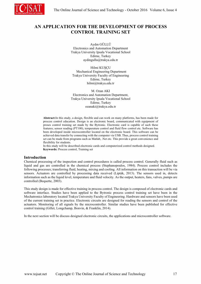
Abstract:In this study, a design, flexible and can work on many platforms, has been made for process control education. Design is an electronic board, communicated with equipment of proses control training set made by the Bytronic. Electronic card is capable of such these features; sensor reading (PT100), temperature control and fluid flow control etc. Software has been developed inside microcontroller located on the electronic board. This software can be achieved data transfer by connecting with the computer via USB. Thus, process control training set can be made from programs such as Matlab, .Net etc. This provide a great convenience and flexibility for students. In this study will be described electronic cards and computerized control methods designed. Keywords: Process control, Training set

Introduction Chemical processing of the inspection and control procedures is called process control. Generally fluid such as liquid and gas are controlled in the chemical process (Stephanopoulos, 1984). Process control includes the following processes; transferring fluid, heating, mixing and cooling. All information on this transaction will be via sensors. Actuators are controlled by processing data received (Lipták, 2013). The sensors used in, detects information such as the liquid level, temperature and fluid velocity. As the output, heaters, fans, valves, pumps are controlled (Bequette, 2003). This study design is made for effective training in process control. The design is composed of electronic cards and software interface. Studies have been applied to the Bytronic process control training set have been in the Mechatronics laboratory located Trakya University Faculty of Engineering. Hardware and sensors have been used of the current training set in practice. Electronic circuits are designed for reading the sensors and control of the actuators. Monitoring of all signals by the microcontroller. Similar studies have been published for effective control training (Gillet, Longchamp, Bonvin, & Franklin, 2014). In the next section will be discuss designed electronic circuits, the applications and microcontroller software.



Material and Method This paper studies will be discussed in two categories namely software and hardware. Hardware; It consists of electrical circuits which is designed and produced. Software is interface, developed on different platforms for process control function.

Figure 1: Process Control Training Set

Electronic Circuit In this study developed electronic circuits for reading the sensor and controlling the actuator on the process control training set. The sensors contained in the system; PT100 temperature meter, analog liquid level meter, flowmeter, limit sensors. The output elements are mixer (DC motors), pump (DC15V), valves (DC 24V), heater (AC220V), radiator coolant -fan (DC24) and lamps. All signals are processed by microcontroller. In addition, the microcontroller communicates with the computer, providing data transfer. Designed circuit will be discussed below. Temperature Measurement (PT100) Pt100 is a sensor, a resistance varying with temperature ("PT100," 2015). 0-100 °C change in resistance is 100-138.51Ω. An operational amplifier (opamp) circuit is designed to read this small change (Ding, 2015). First circuit makes extraction, after than circuit increases signals. There are three PT100 temperature sensor for temperature measurement in training set. There are two of them in two separate tank. The other measures the coolant exit temperature.

Figure 2: PT100 Reading Circuit

Liquid Level Meter Liquid level is measured in the mixing tank. Exchange of the liquid level sensor value is changing linearly. This value is read analog (Jiang & Xiao, 2015). This value is connected to the microcontroller by filtration. It is also made filter in the software. Heater Control 220V 2200W heater is used. Solid state relay used for heater control. Control is done by observing the AC phase



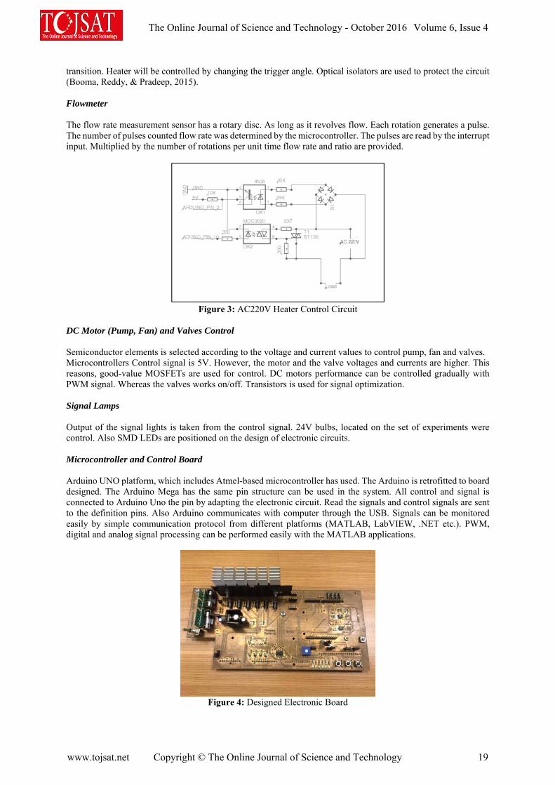
transition. Heater will be controlled by changing the trigger angle. Optical isolators are used to protect the circuit (Booma, Reddy, & Pradeep, 2015). Flowmeter The flow rate measurement sensor has a rotary disc. As long as it revolves flow. Each rotation generates a pulse. The number of pulses counted flow rate was determined by the microcontroller. The pulses are read by the interrupt input. Multiplied by the number of rotations per unit time flow rate and ratio are provided.

Figure 3: AC220V Heater Control Circuit

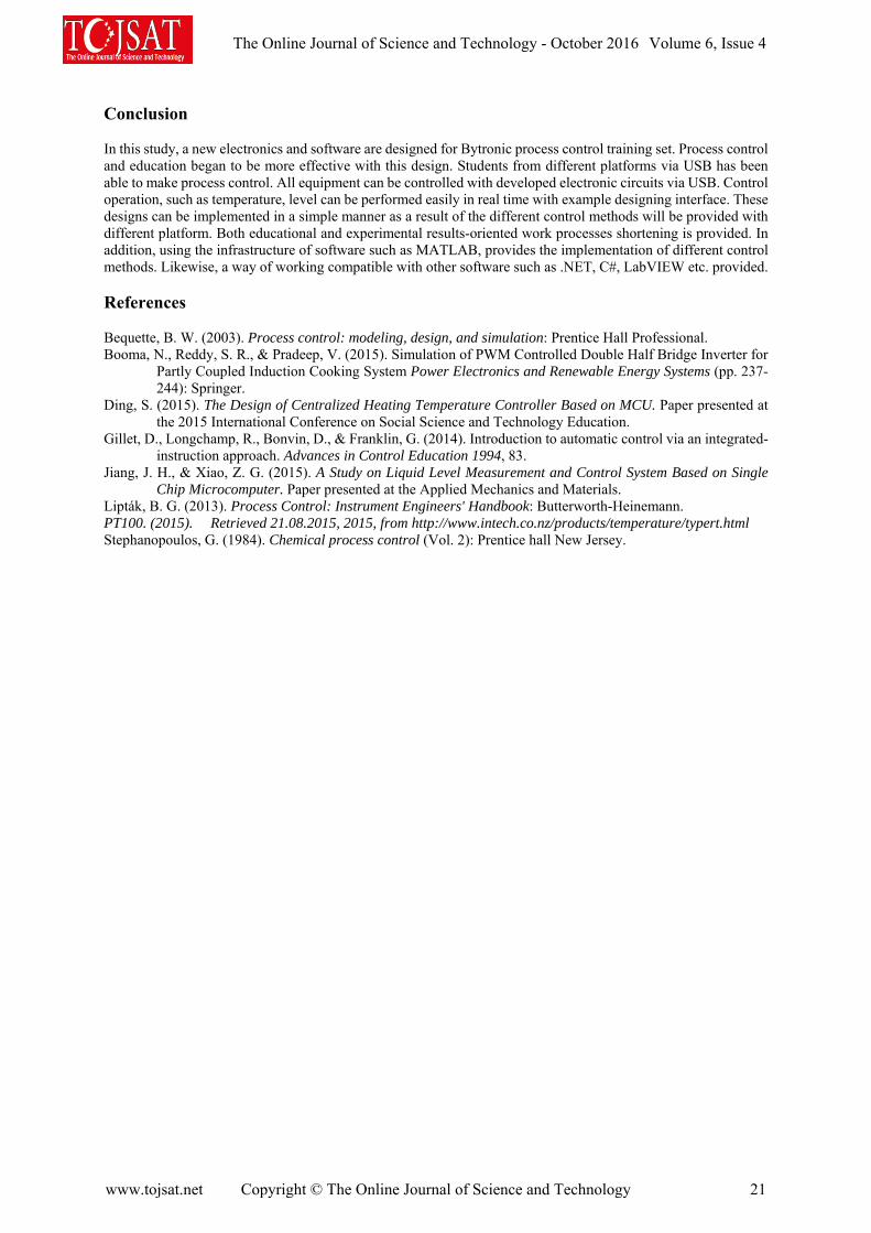
DC Motor (Pump, Fan) and Valves Control Semiconductor elements is selected according to the voltage and current values to control pump, fan and valves. Microcontrollers Control signal is 5V. However, the motor and the valve voltages and currents are higher. This reasons, good-value MOSFETs are used for control. DC motors performance can be controlled gradually with PWM signal. Whereas the valves works on/off. Transistors is used for signal optimization. Signal Lamps Output of the signal lights is taken from the control signal. 24V bulbs, located on the set of experiments were control. Also SMD LEDs are positioned on the design of electronic circuits. Microcontroller and Control Board Arduino UNO platform, which includes Atmel-based microcontroller has used. The Arduino is retrofitted to board designed. The Arduino Mega has the same pin structure can be used in the system. All control and signal is connected to Arduino Uno the pin by adapting the electronic circuit. Read the signals and control signals are sent to the definition pins. Also Arduino communicates with computer through the USB. Signals can be monitored easily by simple communication protocol from different platforms (MATLAB, LabVIEW, .NET etc.). PWM, digital and analog signal processing can be performed easily with the MATLAB applications.

Figure 4: Designed Electronic Board



Software The software consists of two stages. First of them is signal optimization software developed on the Arduino. The other is the control software can be developed on different platforms. Arduino is programmed differently for MATLAB and .NET programs. Switching between these two platforms can be made by means of a jumper. Arduino The Arduino software includes within its scope the following; reading of analog signals, reading of digital signals and to be sent digital signals. It is also made in the mathematical transformation for convenience later, like these data; liquid level, temperature and flow rate. Processed and calculated signals are sent via USB in real-time to program will be used. Again, the signals coming from the program perceived in the Arduino side outputs are controlled. Matlab (Simulink) Software is developed to perform control operations. It allows to quickly control to process the available control blocks located in Matlab. Input and output signals can be taken directly to the Arduino. Also it can be achieved communication via the serial port with improved communication protocol. The same time is used at .NET. The figure below shows the routine for process control fluid level, developed in MATLAB environment.

Figure 5: Matlab Simulink PID Level Control Interface

.Net (C #) As in Matlab interface communication is provided via USB. The required equipment can be controlled by means of visual or console software. For this, there is no need for an additional library. The following figure shows an example for PID temperature control interface.

Figure 6: Heater control interface with C#



Conclusion In this study, a new electronics and software are designed for Bytronic process control training set. Process control and education began to be more effective with this design. Students from different platforms via USB has been able to make process control. All equipment can be controlled with developed electronic circuits via USB. Control operation, such as temperature, level can be performed easily in real time with example designing interface. These designs can be implemented in a simple manner as a result of the different control methods will be provided with different platform. Both educational and experimental results-oriented work processes shortening is provided. In addition, using the infrastructure of software such as MATLAB, provides the implementation of different control methods. Likewise, a way of working compatible with other software such as .NET, C#, LabVIEW etc. provided. References Bequette, B. W. (2003). Process control: modeling, design, and simulation: Prentice Hall Professional. Booma, N., Reddy, S. R., & Pradeep, V. (2015). Simulation of PWM Controlled Double Half Bridge Inverter for

Partly Coupled Induction Cooking System Power Electronics and Renewable Energy Systems (pp. 237-244): Springer.

Ding, S. (2015). The Design of Centralized Heating Temperature Controller Based on MCU. Paper presented at the 2015 International Conference on Social Science and Technology Education.

Gillet, D., Longchamp, R., Bonvin, D., & Franklin, G. (2014). Introduction to automatic control via an integrated-instruction approach. Advances in Control Education 1994, 83.

Jiang, J. H., & Xiao, Z. G. (2015). A Study on Liquid Level Measurement and Control System Based on Single Chip Microcomputer. Paper presented at the Applied Mechanics and Materials.

Lipták, B. G. (2013). Process Control: Instrument Engineers' Handbook: Butterworth-Heinemann. PT100. (2015). Retrieved 21.08.2015, 2015, from http://www.intech.co.nz/products/temperature/typert.html Stephanopoulos, G. (1984). Chemical process control (Vol. 2): Prentice hall New Jersey.



ASSESMENT OF THE USE OF DIATOMITE AND PUMICE IN STONE MASTIC ASPHALT AS STABILIZER

Bekir AKTAŞ, Şevket ASLAN

Department of Civil Engineering, Erciyes University, Turkey

[email protected]; [email protected]

Abstract: Stone Matrix Asphalt (SMA) has been preferred to start because of its better resistance to rutting due to slow, heavy and high volume of traffic. Structure of SMA consists of high coarse aggregate, high asphalt contents and fiber additives as stabilizers. The stabilizing additives generally composed of cellulose fibers, mineral fibers or polymers are added to SMA mixtures to prevent draindown from the mixture. In this study, usability of diatomite and pumice are investigated in SMA as stabilizer. Initially, Marshall samples of SMA mixtures with cellulose fibers with varying binder content are prepared. The optimum binder content is determined keeping the suggested air void content in the mix. Thereafter, the draindown characteristics are studied with diatomite and pumice added SMA mixtures. It is observed that there is a high possibility use of 0.25 % diatomite and 0.20 % pumice in SMA at determined optimum binder as stabilizer. Keywords: Stone Mastic, Asphalt, Stabilizer

Introduction SMA has been accepted to be more advantageous than dense graded mixes for high volume roads. It was firstly developed in Germany in the 1960s, to resist the damage caused by studded tires. As SMA showed good rutting by heavy traffic and high volume roads at high temperatures, its use has been continued even after that. SMA also improved resistance to fatigue effects and cracking at low temperatures, increased durability, reduced permeability and sensitivity to moisture of Hot Mix Asphalts.

SMA has gap graded mixture. This makes it possible for the SMA mixtures to have higher amount of voids. Therefore, stabilizing additives are used in the SMA mixture to prevent bitumen draindown and to provide better binding. Initially, asbestos fiber has been used in SMA successfully. Later, its use was restricted for health and environmental reasons. Nowadays, commonly polypropylene, polyester, mineral and cellulose fibers are used in SMA.

Investigation of alternative stabilizers in SMA mixtures has an important topic for researchers. Waste and natural materials have remarkable potentials for this aim. Brown et al. (1996) studied cellulose, rock wool and slag wool as fiber in SMA. They reported that fibers have a very important role especially at higher temperatures to prevent the draindown of asphalt cement during production and lay out of SMA mixtures. Putman et al. (2004) investigated use of waste tire and carpet fibers in SMA mixtures and compared cellulose fibers. Authors reported that there is no significant difference in permanent deformation or moisture susceptibility between waste fibers and cellulose fibers. They also concluded that tire, carpet and polyester fibers significantly improved the toughness of the mixture than cellulose fibers. Kumar et al. (2007) used jute fibers coated with low viscosity binder as alternative fibers and compared conventional fibers in SMA. Authors concluded that results of strength tests with jute fiber samples comparable to the patented fibers according to Marshall stability tests, rutting test and fatigue life test. They also reported that jute fiber adding samples have better aging index than prepared with patented fibers. In this study two natural materials, dytomite and pumice were used in SMA mixture as stabilizer and investigated draindrown capacity of these materials according to specifications.

Materials and Methods Cellulose fiber Cellulose fiber most commonly preferred in SMA mixtures. The most commonly adopted fibers in SMA mixtures are cellulose fibers. The main component of this fiber is cellulose, a polysaccharide. Cellulose fibers are commonly obtained from plants. It is harmless for human and environment because produced of purely natural cellulose resources. To stabilize the SMA mixture very small amount of cellulose fiber (about 0.3%) is required.



Diatomite Diatomite (kizelgur), formed with the cumulation of the diatom shells and having a composition of SiO2.nH2O, is a light material and it can be easily crumbled. In other words, diatomite is comprised from watermosses and it is an organic solution. Diatomite can be found in the nature easily and its color is generally white. Also, when it is crushed, it changes to a very thin and white-beige dust. This dust has an effect of corrosive and it is light because of its foam-like structure. Diatomite is formed from the fossil of silika and diatom. Diatom is an algae type with hard shells. (Crangle, 2009). The most important features of diatomit are high porosity, low bulk specific gravity and whiteness. When it is dry, the specific gravity is in between 0.15-0.40 g/cm3. Opal hardness in 4.5-6.0 and the hardness of it is not more than 1.5. Generally it is loose and it may be broken by hand easily. The color is light beige, white and sometimes gray. However, the diatomite having rich materials can be brown, dark green or black. (Brady ve Clauser, 1991). Except for the potential areas, it is seen that the reservoir of the World is 2 billion tons. The well-known and biggest diatomite reservoirs are closely located in the Lompoc area, California, USA. The production of diatomite is especially made in USA, France, Spain, Denmark, South Korea, Mexico, Romania and Italy (Breese, 1994). Diatomite, commonly used in all over Turkey, is found especially in Hırka village in terms of size of rezerves. Although the existence of the diatomite material is known since 1900’s, the use of diatomite as a construction material has never been taken into consideration. Pumice There are two types of pumice in the nature. One of them is callded acidic pumice. The other one is called basic pumice. The most common pumice type is acidic pumice. Acidic pumice is also widely used in many areas. The amount of SiO2 determines whether the pumice is acidic or basic. If the amount of SiO2 is increased, this means the pumice is getting more acidic. In this case, as the amount of SiO2 increases, the stability of pumice increases. Moreover, when the amount of Al2O3 is more, it can be said that pumice has more resistancy to fire and heat. In the construction sector, generally it is expected pumice should be acidic and have low amount of Fe2O3 and high

amount of Al2O3. Chemical composition of diatomite and pumice that used in this study are seen in Table 1.

Table 1. Chemical Composition of Diatomite and Pumice

SiO2 Fe2O3 Al2O3 CaO MgO Na2O K2O SO3 KK

Diatomite 85,2 1,85 3,83 1,49 0,45 0,47 0,44 0 0

Pumice 72,03 1,02 12,34 1,09 0,34 5,15 4,62 0,08 3,93 Experimental Work Marshall Test The SMA samples were fabricated according to the Marshall Test procedure specified in ASTM D 6927-06. The coarse, fine aggregates and mineral filler with 0.3 cellulose fiber were mixed according to the Type II gradation as given in Figure 1. SMA samples were prepared in different proportions in the mixes starting from 5.5% to 8.0% with an increasing of 0.5% of the total mix to obtain the optimum binder requirement. After mixing the materials the mixture was poured in to preheated Marshall moulds and the samples were fabricated using a compactive effort of 50 blows on each side. The specimens were kept over night for cooling to room temperature. Then the samples were extracted and tested at 60°C according to the standard testing procedure.



Figure 1. Gradation curve of SMA design

Marshall mix design has been used to determine optimum bitumen content and characterization of bituminous mixes. This design method has also been used to test SMA mixes. Considering Marshall parameters such as Marshall stability, flow value, unit weight, air voids, VMA, VFA optimum binder content of the SMA mixture with 0.3 cellulosic fiber is determined 7.05%. Draindown Test SMA is gap grading hence draindown of binder is a major problem for these mixtures. To learn draindown behavior of SMA is very important to study for SMA mixture. There are many version methods to evaluate the draindown characteristics of SMA mixtures. In this study the Schellenberg draindown test was used. This method commonly used in Europe. It is conducted on approximately 1 kg mixture. The prepared mixture is poured into a 1000 ml glass beaker and weighed. The glass beaker with the mixture is then kept in an oven for 60 minutes at 170°C. Then the mixture is removed from the beaker and placed by quickly turning the beaker upside down without shaking. The final weight of the mixture is taken and the percentage draindown is calculated. Losses greater than 0.3% indicate that segregation problem may be occurred in SMA mix (ASTM D6390, 2011). After determined the optimum binder content of SMA mixture, various amount of diatomite and pumice added mixtures were prepared with optimum bitumen content for draindown test. Diatomite and pumice are added to SMA mixtures as percentages of 0.5%, 1.0%, 1.5% and 2.0% of dry aggregates. Obtained pictures and charts after draindown test are seen in Figure 2.

Figure 2. Remaining materials in the glass beakers after the Schellenberg draindown test



Figure 3. Schellenberg draindown test results of diatomite and pumice added SMA specimens. It is clearly seen in Figures 3, draindown losses without any fiber additives 0.50% which is out of specifications. According to Turkish Highway Specifications, draindown loss using by Schellenberg method is allowed maximum 0.3%. When examined both charts those are diatomite and pumice added samples, it is obtained that a decreasing trend is clearly seen with the increase of stabilizer material. To find possible suitable diatomite and pumice amount regarding 0.3% maximum allowed limit, it can be seen that 0.25% and 0.20% diatomite and pumice can ben use in the SMA mixture respectively. However, it must be noted that other Marshall parameters must be investigated when adding these materials. Conclusions Stone Mastic Asphalt has good rutting performance by heavy traffic and high volume roads at high temperatures. It also has better fatigue resistance and cracking at low temperatures, durability, permeability and sensitivity to moisture than Hot Mix Asphalts. Because of SMA has gap graded mixture, it has higher amount of voids in the mix. Therefore, stabilizing additives are used in the SMA mixture to prevent bitumen draindown and to provide better binding. In this paper, usability of dytomite and pumice are investigated in SMA as stabilizer using by Schellenberg draindown method. According the results there is a high possibility use of 0.25 % diatomite and 0.20 % pumice in SMA at determined optimum binder as stabilizer. However, it must be noted that other Marshall parameters and performance characteristics of SMA must be investigated when adding these alternative stabilize materials.

References ASTM D 6927 (2006). Standard test method for Marshall Stability and flow of bituminous mixtures., West

Conshohocken, PA ASTM D6390 (2011). Standard Test Method for Determination of Draindown Characteristics in Uncompacted

Asphalt Mixtures, ASTM International, West Conshohocken, PA. BRADY G. S.,1991, Clauser, H. R., “Materials Handbook”, Mc Graw, New York BREESE R.O.Y., 1994, Diyatomite, Industrial Minerals and Rocks, Carr (Ed), 397-412, Colarado, USA.. Brown E.R., Haddock J.E. and Crawford C. (1996), “Investigation of Stone Matrix Asphalt Mortars”, TRR 1530,

National Research Council, TRB, USA, pp 95 ±102 Crangle, R.D., Jr., 2010, Diatomite: U.S. Geological Survey Mineral Commodity Summaries 2010. Kumar Pawan, Chandra Satish and Bose Sunil (2007), 'Laboratory Investigations on SMA mixes with Different

Additives', International Journal of Pavement Engineering, Volume 8, Issue1, pp 11-18 Putman B.J. and Amirkhanian S.N. (2004), “Utilization of Waste Fibers in Stone Matrix Asphalt Mixtures”,

Resources, Conservation and Recycling, Volume 42, Issue 3, pp 265-274

y = -1.643,88x3 + 69,12x2 - 0,97x + 0,01R² = 0,99

0,00%

0,10%

0,20%

0,30%

0,40%

0,50%

0,60%

0,0% 0,5% 1,0% 1,5% 2,0%

Dra

ind

own

Los

s

Rate of Diatomite

y = -2.621,03x3 + 99,67x2 - 1,16x + 0,01R² = 0,98

0,00%

0,10%

0,20%

0,30%

0,40%

0,50%

0,60%

0,0% 0,5% 1,0% 1,5% 2,0%

Dra

ind

own

Los

s

Rate of Pumice



AUTOMATIC GENERATION OF CONFUSABLE SETS IN SMART SPELL CHECKING FOR KOREAN LEARNERS OF ENGLISH

Kong Joo Lee & iJee Eun Kim

Dept. of Information Communications Engineering Chungnam National University, Korea

[email protected] i Dept. of English Linguistics

Hankuk University of Foreign Studies, Korea [email protected]

Abstract: This paper presents an automatically generated English confusable word set to be used for smart spell checking. A confusable set includes pairs or subsets of frequently misused English words. When Koreans learn English as L2, they produce various types of errors, some of which are caused by negative language transfer. The language system of Korean interferes with English which results in creating a peculiar system. In particular, Korean and English present distinct phonetic and phonemic inventories from each other. The distinctions influence not only the pronunciation of a word, but also its spelling. For certain types of spelling errors, smarter suggestions can be provided when a confusable set is modified for Korean learners. The Double Metaphone algorithm is adopted and revised to implement the phonetic and phonemic properties of Korean. The result is used to automatically generate a confusable set which provides customized suggestions to be used in spell checking. Keywords: Smart Spell checking, Korean learner, English

Introduction Spell checking techniques become smarter as human language technology develops. Its fundamental algorithm is to check whether a word is known and correctly spelled. A word in its use is supposed to be identical to the lemma or one of its morphologically legitimate variants. When the word is not identified as one of those forms, it is determined as an error. When an error is detected, the spell checker suggests a list of candidates to correct the error, which is generated based on the dictionary entries and various heuristics. Semantically anomalous errors, however, cannot be identified as an error because they are spelled correctly and the error detecting scope is beyond the capacity of the spell checker. These errors are legitimate dictionary entries and occur in a morphologically grammatical form. They are classified as usage errors which occur when a word does not fit in the context. This type of errors can be resolved effectively by utilizing a confusable word set. Usage errors are produced by the following causes: people choose an inappropriate word because a) they are unfamiliar with the word implying the intended meaning, b) they are not certain of the contextually appropriate form of the word, and c) they are confused with the spelling or the pronunciation of the word in question. These types of errors can be detected only when the scope of spell checking expands to the context from a single word.

1) Our holiday house is among/between the mountains and the sea. The ancient fountain was hidden among/between the trees.

2) Can I borrow/lend your dictionary? I never borrow/lend my books to anyone.

In example 1) and 2), only one of the underlined words is grammatical in the context although they are semantically related and occur in an appropriate form with the correct spelling. The underlined pair of words in example 1) implies the same meaning, but one has to be selected depending on the quantity of the following noun phrase. The pair in example 2) is also semantically related, but in antonymic relation. A word of the pair can be chosen only when the intended meaning of the sentence is comprehended. In other words, selecting an appropriate word is context-sensitive in both examples. In order to detect these types of errors, the speller needs to figure out the contextual meaning of the word, which requires expanding the scope of the speller, from a single word to a bigger unit such as a phrase or a sentence.



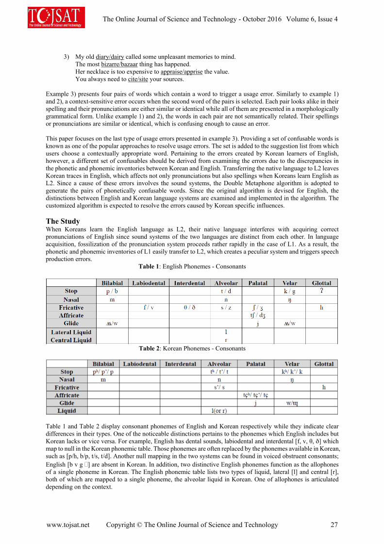
3) My old diary/dairy called some unpleasant memories to mind.

The most bizarre/bazaar thing has happened. Her necklace is too expensive to appraise/apprise the value. You always need to cite/site your sources.

Example 3) presents four pairs of words which contain a word to trigger a usage error. Similarly to example 1) and 2), a context-sensitive error occurs when the second word of the pairs is selected. Each pair looks alike in their spelling and their pronunciations are either similar or identical while all of them are presented in a morphologically grammatical form. Unlike example 1) and 2), the words in each pair are not semantically related. Their spellings or pronunciations are similar or identical, which is confusing enough to cause an error. This paper focuses on the last type of usage errors presented in example 3). Providing a set of confusable words is known as one of the popular approaches to resolve usage errors. The set is added to the suggestion list from which users choose a contextually appropriate word. Pertaining to the errors created by Korean learners of English, however, a different set of confusables should be derived from examining the errors due to the discrepancies in the phonetic and phonemic inventories between Korean and English. Transferring the native language to L2 leaves Korean traces in English, which affects not only pronunciations but also spellings when Koreans learn English as L2. Since a cause of these errors involves the sound systems, the Double Metaphone algorithm is adopted to generate the pairs of phonetically confusable words. Since the original algorithm is devised for English, the distinctions between English and Korean language systems are examined and implemented in the algorithm. The customized algorithm is expected to resolve the errors caused by Korean specific influences. The Study When Koreans learn the English language as L2, their native language interferes with acquiring correct pronunciations of English since sound systems of the two languages are distinct from each other. In language acquisition, fossilization of the pronunciation system proceeds rather rapidly in the case of L1. As a result, the phonetic and phonemic inventories of L1 easily transfer to L2, which creates a peculiar system and triggers speech production errors.

Table 1: English Phonemes - Consonants

Table 2: Korean Phonemes - Consonants

Table 1 and Table 2 display consonant phonemes of English and Korean respectively while they indicate clear differences in their types. One of the noticeable distinctions pertains to the phonemes which English includes but Korean lacks or vice versa. For example, English has dental sounds, labiodental and interdental [f, v, θ, ð] which map to null in the Korean phonemic table. Those phonemes are often replaced by the phonemes available in Korean, such as [p/h, b/p, t/s, t/d]. Another null mapping in the two systems can be found in voiced obstruent consonants; English [b v g ] are absent in Korean. In addition, two distinctive English phonemes function as the allophones of a single phoneme in Korean. The English phonemic table lists two types of liquid, lateral [l] and central [r], both of which are mapped to a single phoneme, the alveolar liquid in Korean. One of allophones is articulated depending on the context.



Because of the differences in the language systems, the Korean language interferes with learning English, which is known as negative language transfer in L2 acquisition. Flege(1987) claims that the L2 learners classify the sounds of L2 based on the L1 sound system, which may result in a new and peculiar system. Accordingly, the resultant system induces various types of production errors. Jang(2005) has categorized the sounds produced by negative language transfer which progresses while Koreans learn English. Since he focuses on speech including phonetic and phonemic representations, the classification has to be revised to include the relation between the pronunciations and the spellings. The main goal of this research is to provide a set of Korean pronunciation influenced confusable words for spell checking. Since a confusable set by definition is composed of approximately suitable words to be used as suggestion candidates, mapping between the scripts and their pronunciations has to be redefined, also considering the errors produced by Korean learners. In order to customize the set for Koreans, the Double Metaphone algorithm is adopted and revised to satisfy the research need. Double Metaphone refers to the second generation of phonetic encoding algorithm designed for indexing English words according to their pronunciations. The goal of the original algorithm is to reduce the discrepancies between the spelling and pronunciation of English words. The algorithm is found to be effective in identifying words with similar pronunciations. In addition, Double Metaphone is known for working best with recognizing proper names. Even native speakers of English produce different pronunciations for the same name, which frequently results in spelling errors when converting the speech to the text. More than one acceptable pronunciation can be mapped to a proper name. The Double Metaphone algorithm is designed to allow dual scripts for a single string, primary and secondary encodings in order to capture those script variants and an ambiguity which the string may presents in terms of its pronunciation. The algorithm adopts a single representative script for similar sounds. It attempts to encode all the English words using four consonant metaphones to the maximum, ignoring vowels although the number of metaphones can be adjusted as necessary.

Table 3: English Primary Encoding in Double Metaphone

ALPHABET PRIMARY ALPHABET PRIMARY a/e/i/o/u/y A (at first position)

ignore (others) n N

b P p P or F(ph) c K(chorus) or S(caesar) or

X(chair) or KS(accident) q K

d J(edge) or TK(edgar) or T(width) r R f F s X(sugar) or S(smith) or SK(school) g K(baggy) or J(agile) or F(cough) or

KN(ignite) or N(gnarl) or KL(glide) t T or X(tion) or 0(th)

h H v F j J(jet) or H(Jose) w R(wr-) or A(Womo) or

TS(filipowicz) or F(Arnow) k K x S(first character) or

ignore or KS(breaux) l L z S or J(Zhang) m M

Table 3 presents the representative primary encoding for each English alphabet while summarizing the encoding rules of the algorithm. Some of the alphabets such k and m are mapped to a single pronunciation. In other cases, an alphabet is represented with multiple metaphones encoding similar pronunciations. For example, a letter c is represented by 4 different metaphones including K, S, X or KS depending on its pronunciation within a word.



Table 4: English Double Metaphone Examples

METAPHONE

PRIMARY ENCODING EXAMPLES

FNRL venereal, funereal, funeral FN fawn, feign, finny, vino, vain, vine, faun, fain, fine, funny, van, fen, fin, von,

phony, phone, fan, vein, venue, fanny, fun, vane, fauna PST basset, past, best, bust, beside, baste, boost, biocide, bast,

paucity, bestow, beast, pasta, post, paste, beset, peseta, boast, pest, posit, pasty FTLT futility, vitality, fatality, fidelity, feedlot KKTR cockatrice, coquetry FNN vinyon, phonon SNTF centavo, cenotaph, scientific, sendoff

Table 4 displays examples generated utilizing Double Metaphone primary encoding described in Table 3. It also shows the pairs of words which share the same metaphone encodings. Native speakers of English often produce pronunciation errors by articulating the counterpart of a sound, with the same phonetic features but voicing. Two consonant phonemes, p and b are encoded as P since they are identical in their articulatory properties except for voicing. For example, pest is frequently pronounced when bast is intended. This confirms that native speakers of English tend to get confused with voicing. Findings The coverage of the Double Metaphone algorithm has to be expanded to add a set of Korean influenced confusable words since the algorithm is intended for the sake of the native speakers or the experts of English. In order to add Korean specific rules to the algorithm, the errors produced by Korean learners have been examined. One of the most noticeable errors is incorrectly used English liquids. The Korean phonemic system includes a single liquid which allows two allophones mapped to the two distinctive liquids, lateral and central in the English system. Korean allophonic distinctions of the liquid can be recognized by considering the context; the central liquid is pronounced at the syllable initial position whereas the lateral is articulated elsewhere. Since the Korean liquids are not phonemically distinctive, Koreans often fail in distinguishing one English liquid from the other. For example, the pairs of words such as right/light and lead/reed are pronounced the same, selecting either one of the pair. Another difference of worth noticing is that voiced obstruent consonants are not available in the Korean sound system, which enforces the learners to replace them with their voiceless counterparts. For example, [p] is articulated for [b] as in [pai] pronounced for buy. Similarly, English dental sounds are replaced with Korean phonemes which are not very phonetically similar. For example, [v] in veil is articulated as [b] and [f] in fight is pronounced as either [p] or [hw]. Not all of the distinctions in the phonetic/phonemic inventories, however, result in spelling errors. Null mapping to English voiced obstruents causes speech errors depending on the position. Only a word initially occurring voiced obstruent is frequently replaced with its voiceless counterpart. For example, a word gag is often pronounced as [kag]; a word initially occurring [g] as tends to be pronounced as [k] whereas the word final g usually remains as [g]. However, this particular phonemic gap between the two systems does not seem to interfere with spelling L2 words. With considering the characteristics of various Korean influenced pronunciation errors, the Double Metaphone algorithm is revised to provide an effective confusable set. In order to minimize the revision, only the secondary encoding is modified while adopting the primary as is.

Table 5: Korean Encoding in Double Metaphone

ALPHABET PRIMARY ENCODING

(Original Metaphone) SECONDARY ENCODING

(Modified For Korean) f F F v F B b P B p P F l L L r R L



Table 5 presents the changes in the secondary encoding to represent the influence of Korean pronunciation on English. A metaphone B is added to map v and b and L to represent r. Based on the revision with the secondary encoding, an algorithm is created to check whether a word is qualified for one of the confusable pair.

Table 6: Algorithm to Determine Confusables

IsConfusable(word a, word b) if metaphone(a) == metaphone(b)

and minimum_edit_distance(a, b) < Threshold and hasSameStem(a,b) == False: return True;

Table 6 presents a function called IsConfusable(word a, word b) describing the procedure to check whether the two input words, a and b compose a confusable pair. They are determined as a pair if they satisfy all of the following conditions: 1) their metaphone encodings are identical, 2) their minimum edit distance is less than the threshold, and 3) they do not share the same stem. The embedded function hasSameStem(a, b) checks their stems and returns ‘True’ when they have the same stem. For example, given with the two words, replicate and replicator, the function IsConfusable returns “False” determining that they are not a confusable pair. They have the same metaphone encoding and their minimum edit distance is below the threshold. However, they share the same stem replicate, which enforces the embedded function to return ‘True’.

Table 7: Confusable Words for Korean Learners of English

CONFUSABLES FOR ENGLISH USING PRIMARY ENCODIGN

FOR KOREAN USING SECONDARY ENCODING

COMMON

base, past bast, past fine, vine rebel, repel

fast, past fine, pine bast, vast rebel, revel

PRIMARY ONLY (English Speakers)

funereal, venereal backing, packing backoff, pickoff fatality, vitality file, vile

SECONDARY ONLY

(Korean Speakers)

bane, vane bang, vang flat, plat read, lead lace, race lasting, resting lavish, ravish level, revel

Table 7 presents a set of confusable words produced as the output of the current research. The confusables are automatically generated using the algorithm described in Table 6. The first column lists the pairs of confusable words generated by implementing the original primary encoding of Double Metaphone while the second column displays the pairs for Koreans produced utilizing the secondary encoding. The row led by COMMON displays the pairs of confusables which can be shared by both English and Korean speakers. The pairs in the PRIMARY ONLY row are the words generated solely for English speakers. The row with SECONDARY ONLY presents the confusables which Korean speakers would benefit from. Table 7 suggests clear differences between English and Korean regarding the types of confusables. For example, English speakers mistake fine for vine or vice versa, from which the misused phoneme can be predicted using English phonetic/phonemic features. In addition to this confusable pair, Korean speakers get confused with fine for pine more often, which is created by the influence of Korean phonetic/phonemic system. Unlike the English pair, the replaced phoneme such as [p] for [f] cannot be predicted while causing frequent spelling errors. Accordingly, the customized confusables for Koreans are expected to be effective in providing refined suggestions for common spelling errors when they are added to the existing list in spell checking. Similarly, smart spell checking implemented with context-sensitivity can suggest revel over repel for an error rebel since, for Korean speakers, confusion between the pair, rebel/revel causes a usage error more frequently than the pair rebel/repel. In addition, the speller can provide an updated pair, read/lead, for another common usage error.



Conclusions This paper has introduced an automatically generated confusable set to be implemented in smart spell checking. The set is created utilizing the customized Double Metaphone algorithm for Korean learners of English. Double Metaphone is useful in capturing the representative scripts of an alphabet which may be mapped to multiple pronunciations caused by either phonological convention of English or speech production errors. Mapping multiple pronunciations to a single metaphone is effective in creating a set of confusables to be used as suggestion candidates in spelling checking. Since Koreans produce different sets of pronunciation errors from those made by native speakers of English, the secondary encoding in the Double Metaphone algorithm is complemented with a list of confusable words customized for Koreans. Implementing the modified algorithm in spell checking is expected to provide an improved set of suggestion candidates. Additionally, the revised Double Metaphone algorithm can be adopted to create a suggestion list for proper names whose spelling may be confusing or unknown. For example, a smart speller implemented with the algorithm can suggest Pausini for Fausini inputted by a Korean to search an Italian singer Laura Pausini while Vausini would be a more effective candidate to be paired with Pausini for English speakers. As the next step of the research, the revised algorithm will be implemented to generate accurate spellings of proper names which are known only with their pronunciations. It is expected to be useful since spelling proper names is often difficult for the learners of English as well as the native speakers. The performance accuracy will be evaluated in comparison with different approaches. Acknowledgements This work was supported by Hankuk University of Foreign Studies Research Fund of 2015. ReferencesFlege, J. E. (1987) The production of new and similar phones in a foreign language: evidence for the effect of

equivalence classification, in Journal of Phonetics. 15: 47-65. Fromkin, V., R. Rodman & N. Hyams (2011). An Introduction to Language. 9th ed. Wadsworth. Jang, T. Y. (2005). Construction of an English speech database for Korean learners of English", Language and

Linguistics, Vol 35: 293-310. Language Research Institute. Hankuk University of Foreign Studies. (in Korean)

Phillips, Lawrence (1990). "Hanging on the Metaphone", Computer Language, 7(12). Phillips, Lawrence (2000). "The Double Metaphone Search Algorithm", C/C++ Users Journal, 18(6). The Soundex Algorithm, available online at

http://www.archives.gov/research_room/genealogy/census/soundex.html UzZaman, N., & M. Khan (2005). A double metaphone encoding for Bangla and its application in spelling

checker. In Natural Language Processing and Knowledge Engineering, 2005.

i Corresponding author.



CLASSIFYING HAND SIGNS USING IMAGE PROCESSING

Ozan AKI Trakya University

Turkey [email protected]

Aydın GÜLLÜ

Trakya University Turkey

[email protected]

Abstract: In this study, we aimed to classifying basic hand signs with image processing techniques. Hand images were obtained from a camera and each signs were classified manually for creating learning samples. Gabor wavelets were used to extract features of each hand sign image. Meaningful features were selected for teaching machine learning algorithms while weak features were rejected. Some well-known machine learning algorithm results were compared and best one were selected for real time testing. Keywords: Hand Sign, Image Processing

Introduction Hand movements and hand signs has become a novel way to interact smart devices. Many time these methods are just funny and alternative ways to use devices such computers, smartphones, smart TV sets and game consoles. But on the other hand, these alternative interact methods may aid patients, disabled people, machine operators. Patients may call nurse by simply a hand gesture. Disabled people may call elevator by a hand movement. Machine operators may work safely by checking if hands are in safe. In this study, we aim to classifying some specific hand shapes by using image processing and machine learning techniques. Hand shape images obtained by a webcam camera. Each shape of hand images were extracted from live video stream and saved as images with different orientation and different variations. We stored each hand shape images in named subfolder. After collecting all classified images, developed application was calculate Gabor wavelet transformation for all images and built an ARFF (Attribute Related File Format) file using by Weka (Machine Learning Group at the University of Waikato) machine learning application. ARFF file format was used for selecting meaningful features and evaluating machine learning algorithms. Finally, most successful machine learning algorithm was selected by comparing each other. Materials and Methods Image Database In this study, only five group of specific hand shape images were used. For simplicity, each group of hand shape shows numbers with fingers. Hand shape images were obtained from solid black background platform using Microsoft LifeCam camera. Sample images were grabbed from camera every 10 frame interval with different angle and variations. Thus total 1569 images collected. Each group has 300 images approximately.

Figure 1: Hand shape groups that indicate numbers

Each group of hand shape images will used for machine learning afterwards. Thus hereafter each group will be called as class. Each classes of hand shape images were saved in sub-folders that named as class name. Thus, hand shape images database were created. Feature Extraction



Image processing consists of several stages. Preparing images for processing is the first stage. In this stage, Gaussian filter has been applied to images for reducing noises. Then these images has been converted to grayscale that contains only illumination information instead colors (Bradski & Kaehler, 2008). Thus, image database has been prepared for feature extraction processes. Gabor filters, in other words Gabor wavelet transforms can extract time and frequency information from multi-dimensional signals like images. Also multi-resolution analysis can be done with adjustable kernel sizes. Gabor filters are mostly using in image processing applications such as facial expression classification, face recognition, texture classification (Chao, 2011; Ilonen, Kämäräinen, & Kälviäinen, 2005). A two dimensional Gabor wavelet defined as in Equation 1 and Equation 2.

, ∙∙

∙ (1)

, ∙∙

∙ (2)

Where , defines center frequency and , the spread of the Gaussian window (Derpanis, 2007).

Figure 2: Eight angles and five scale Gabor kernel images

In this study, Gabor wavelet transforms were used for extract features of images for learning and classification. Five different scale for eight different angle (0°, 22,5°, 45°, 67,5°, 90°, 112,5°, 135°, 157,5°) Gabor kernels has been calculated for each images. Gabor kernels were shown in Figure 2. Convolving each kernel with image results real, imaginary, amplitude and phase components. Thus 160 feature per image has been calculated.

Figure 3: Input image convolving with Gabor kernel

Gabor wavelet transforms are calculating by convolving whole image with Gabor kernel and resulting an image. Figure 3 shows a result of convolving input image with a specific Gabor kernel. Each kernel transforms calculates separately for an image. Developed application scans all sub directories and calculates all 160 feature for each image automatically. At the same time, this application builds an ARFF file that each calculated image features has been a data line. ARFF files are using by Weka application for machine learning processes (M. Hall et al., 2009). Figure 4 shows developed application's screen capture while working. This application detects number of core of CPU (Central Processing Unit) and processes same number of images concurrently.



Figure 4: Developed application for automated feature extraction

Machine Learning Machine learning is simply described as turning data into information (Bradski & Kaehler, 2008). For doing this, machine learning looks for patterns within data by training and afterwards we can ask questions about new upcoming data never seen before (Witten & Frank, 2005). Classifiers are machine learning algorithms. These algorithms are using for classifying unknown data based on trained data before. Evaluation of classifiers results some metrics. Most of these metrics calculates from confusion matrix. Confusion matrix shows number of correctly and incorrectly classified data for each classes. In confusion matrix, number of correctly classified positive data are called as TP (True Positive) and number of incorrectly classified positive data are called as FP (False Positive). Similarly, number of correctly classified negative data are called as TN (True Negative) and number of incorrectly classified negative data are called as FN (False Negative). Hereby, accuracy is calculated as in Equation 3.

(3)

Accuracy shows percentage of correctly classified instances both positive and negative (Kılıçaslan, Güner, & Yıldırım, 2009). Precision is calculating as in Equation 4.

(4)

Precision rate shows errors which are caused by classifying negative instances as being positive (Kılıçaslan et al., 2009). Recall is calculating as in Equation 5.

(5)

Recall rate shows errors which are caused by classifying positive instances as being negative (Kılıçaslan et al., 2009). f-measure is calculating as in Equation 6.

∙ ∙

(6)

The f-measure combines precision and recall by calculating their harmonic mean (Kılıçaslan et al., 2009). ROC (Receiver Operating Characteristic) area is a calculated area under curve that plot recall versus FPR (False Positive Rate). FPR is calculating as in Equation 7.

(7)

Gabor wavelet transformation results used for evaluation some well-known classifiers. Weka (version 3.6.11) application were used for evaluation of machine learning algorithms. Weka is an application that have collection of machine learning algorithms for data mining tasks (M. Hall et al., 2009).



Results and Conclusions Gabor wavelet transforms or Gabor filters are useful for extract image features. In this study, all possible Gabor kernels were used for experimental purposes. Extraction all possible features from all images needs much processor power and takes much longer time. Using all possible features will not be practical for real time classifying. For efficient calculation and saving time, less-meaningful features can be ignored. Therefore, there are two different experiments in this study. In the experiment 1, all the features that total of 160 were calculated for each image in the image database. In the experiment 2, only selected features that total of 34 were calculated for reduce computing time. Features were selected by using CFS (Correlation-based Feature Selection) attribute evaluator and best first search algorithm with default parameters in Weka application (M. A. Hall, 1999). Results of experiment 1 and experiment 2 and difference between experiments were shown in Table 1. All classifiers were used with default parameters as defined in Weka application. Cross-validation fold was used as 10. Only high rated classifiers were accepted for comparing.

Table 1: Evaluation of classifiers

Classifier Experiment Accuracy

(%) Precision Recall f-Measure Kappa ROC Area

Naïve Bayes 1 81.47 0.820 0.815 0.814 0.7644 0.972 2 88.09 0.885 0.881 0.880 0.8491 0.986 ∆ +6.62 +0.065 +0.066 +0.066 +0.0847 +0.014

IBk 1 99.49 0.995 0.995 0.995 0.9935 0.998 2 99.30 0.993 0.993 0.993 0.9911 0.996 ∆ -0.19 -0.002 -0.002 -0.002 -0.0024 -0.002

J48 Decision Tree

1 96.56 0.966 0.966 0.966 0.9564 0.984 2 95.92 0.959 0.959 0.959 0.9483 0.982 ∆ -0.64 -0.007 -0.007 -0.007 -0.0081 -0.002

RBF Network 1 93.82 0.939 0.938 0.938 0.9217 0.987 2 95.92 0.959 0.959 0.959 0.9483 0.993 ∆ +2.10 +0.02 +0.021 +0.021 +0.0266 +0.006

Bagging 1 97.77 0.978 0.978 0.978 0.9718 0.998 2 96.88 0.969 0.969 0.969 0.9605 0.998 ∆ -0.89 -0.009 -0.009 -0.009 -0.0113 0.000

Random Forest

1 98.98 0.990 0.990 0.990 0.9871 0.999 2 98.85 0.989 0.989 0.989 0.9855 0.998 ∆ -0.13 -0.001 -0.001 -0.001 -0.0016 -0.001

By ignoring eliminated features with selection algorithm, Naïve Bayes and RBF Network classifiers’ accuracy were increased while others decreased. When inspecting the changing rates of accuracies, it is evident that the decreasing accuracies' changing rates are quite small. On the other hand, serious computation power savings (78.75%) are obtained by reducing number of features from 160 to 34. By inspecting Table 1, most accurate classifier is IBk algorithm and can be used for real time testing with only selected attributes. References Bradski, G., & Kaehler, A. (2008). Learning OpenCV: Computer vision with the OpenCV library: " O'Reilly

Media, Inc.". Chao, W.-l. (2011). Gabor wavelet transform and its application. R98942073. Derpanis, K. G. (2007). Gabor filters. Hall, M., Frank, E., Holmes, G., Pfahringer, B., Reutemann, P., & Witten, I. H. (2009). The WEKA data mining

software: an update. ACM SIGKDD explorations newsletter, 11(1), 10-18. Hall, M. A. (1999). Correlation-based feature selection for machine learning. The University of Waikato. Ilonen, J., Kämäräinen, J.-K., & Kälviäinen, H. (2005). Efficient computation of Gabor features: Lappeenranta

University of Technology. Kılıçaslan, Y., Güner, E. S., & Yıldırım, S. (2009). Learning-based pronoun resolution for Turkish with a

comparative evaluation. Computer Speech & Language, 23(3), 311-331. Witten, I. H., & Frank, E. (2005). Data Mining: Practical machine learning tools and techniques: Morgan

Kaufmann.



COMPUTATIONAL DESIGN OPTIMIZATION OF ROAD SPEED BUMPS

Hakan ERSOY, Kayra KURŞUN

Akdeniz University Mechanical Engineering Department, Antalya, Turkey [email protected]

Abstract:In this study, for urban traffic control; several speed bump forms are proposed as novel designs by the usage of design optimization algorithm. A generic automobile suspension and standard speed bump relations are modeled as dynamic systems and processed in a computerized simulation. In established simulation model, the speed bump form is assumed as road input and its cross section curve is polynomial. The optimization algorithm minimizes the vehicle oscillation when the vehicle passes over the speed bump within the range of determined speed limits and elevates the vehicle oscillation to a safe but higher pre-defined value when the vehicle passes over the speed bump with much higher speeds. Optimization is carried out by entering the required parameters to design optimization toolbox and the obtained simulation and optimization values provides different speed bump forms for different speeds. Keywords: Road Speed Bump, Computational Design

Introduction The increase of the human population in cities lead to congestion of the urban traffic elements. Also it is an indisputably fact that the unavoidable increase in the count of motorized vehicles impacts this situation badly. When any component within a system causes this much concentration, some variety of methods, rules and protocols must be established in order to regulate their relations with each other. Therefore when this situation considered under the traffic regulations, the thing that first comes to mind is general traffic rules. But determining regulators of this rules cannot enforce these effectively all the time, so some enforcing precaution applications must be developed. To control motorized vehicles - mostly automobile speeds in urban areas, some mandatory speed reducing methods are applied on several roads. These are called traffic calming devices and there are several different types such as speed humps, speed bumps, raised intersection, raised pedestrian crossings, chokers etc. Speed bumps or humps are much widely used comparing to others. However, commonly used speed bumps hardly fulfill their functions on applied roads. The expected functions from these devices are; when vehicles pass them over at the speed limit or lower, there should not be very high amplitude and / or very high frequency oscillations on the vehicle body, so the passengers and the driver feel little discomfort and when vehicles pass them over with a speed higher than the limit, there will be considerable discomfort level but those oscillations amplitude and frequencies should not be as high as they could cause injuries on the passengers. However this is hardly the case. Even if vehicles pass some types of this bumps over with very low speeds for speed limits, there could be some high level of discomfort. Contrarily to this situation, when vehicles pass same type bumps over with high speeds than the limit, passengers could feel much less discomfort. Apart from these problems, if a driver realizes these bumps at the last moment, they could break suddenly or could not break at all and vehicles could pass over some bumps unbalanced or passengers in an unexpected sitting position could experience sudden vertical accelerations. As a result of these, accidents and variety form of injuries may occur. Besides, drivers who realize these problems develop a bad driving habit which is slowing down swiftly while approaching a bump and as soon as vehicle passes over the bump accelerating at once. This driving cycle increases fuel consumption and the release of harmful emission gases compared to normal driving. In order to solve these problems some design propositions are made in the literature by researchers. Moreno et. al. (2012) developed a novel traffic calming device which is called speed kidney and by this design it is aimed that general problems with current designs can be minimized. As the name suggests, this device is a kidney-shaped speed hump. If a vehicle passes over this hump with a straight path, one or two wheels of the vehicle passes over the hump. After that, the driver and the passengers would experience discomfort. Therefore driver would be forced to slow down the vehicle. On the other and if vehicle passes the hump with a curved path with an appropriate speed which is close the limit, there would be no discomfort. By this maneuver, discomfort levels can be reduced on speed limits and other negativities can be prevented. Pedersen (1998) optimized the shape of a speed bump (sleeping policeman) with respect to the response characteristic of a car going over the bump. The shape of the bump is controlled by amplitudes of basic functions that are orthogonal in the sense that each contributes something



new to the design space. Optimization is performed with numerical sensitivities, from a planar multibody system simulation. Khorsid and Alfrared (2004) proposed an optimum speed hump design by using second degree sequential programming method. Dynamic behavior of the automobile and drive components are theoretically inspected while the vehicle passing over the hump and vehicle – passenger model is presented as a 12 degrees of freedom mathematical model. A comfort criteria is defined for comfortable or uncomfortable drive, and it is modeled using driver’s vertical head acceleration. Three types of humps are discussed and evaluated in the optimization technique. These humps are Watts, flat-topped and polynomial humps. The global design is selected from 42 optimal designs which are found by combining different rise/return profiles for the three types of humps. Ardeh et. al. (2008) proposed an approach which is based on multiobjective genetic optimization of the hump profile. A 6-degree of freedom non-linear dynamic model is used to identify the speeds at which separation occurs, and three independent objective functions are selected for optimization. As a result, two optimal designs were found and a Pareto front of at least ten optimal points is achieved for each of the two hump profile types.

The Study In this study, first of all 5 degrees of freedom mathematical model is created (Figure 1). To solve the differential equations which are obtained from the model, the boundary conditions should be determined.

Figure 1. 5 degrees of freedom dynamic half automobile model

The dimensions of 45 mm x 600 mm (height x width) standard PVC speed bump as vertical coordinates, and the passing over the bump times at different velocities of 30 km/h, 50 km/h and 70 km/h as horizontal time coordinates inserted to the curve fitting algorithm. As a result of evaluating this algorithm three different form of input Cartesian coordinate groups are obtained as curve graphics (Figure 2).

Figure 2. The input signals



Equations of motions derived from Newton’s second law are given below. Vertical movement of the vehicle body on the front wheels:

(1)

Vertical movement of the unsprung mass on the front wheels:

(2)

Vertical movement of the vehicle body on the rear wheels:

(3)

Vertical movement of the unsprung mass on the rear wheels:

(4)

The numerical values of these parameters are given below (Table 1).

Table 1. The numerical parameter values which are used in the 5 degrees of freedom automobile model Parameter Verbal equivalent Value

Vehicle mass on the front wheels 300 kg Unsprung mass on the front wheels 70 kg Vehicle mass on the rear wheels 300 kg Unsprung mass on the rear wheels 60 kg Spring constant of the front suspension 25000 N/m Spring constant of the front wheels 200000 N/m Spring constant of the rear suspension 22000 N/m Spring constant of the real wheels 180000 N/m Damper constant of the front wheels 1900 N.s/m Damper constant of the real wheels 1600 N.s/m Front suspension distance from center of gravity 1.2 m Rear suspension distance from center of gravity 0.9 m Road input Polynomial signal

Findings The simulation of the mathematical model carried out for 4 seconds, and the graphical results of vertical displacements for different velocity values are shown at figures 3, 4 and 5.

Figure 3. Vertical displacement of a vehicle which passes over a standard bump with a velocity of 30 km/h





At the last phase of this study, an optimization algorithm developed based on vertical displacement results. For this algorithm, non-linear dynamic system parameters inserted into the design optimization technique. This technique uses least squares method to solve curve fitting problems as shown below. ‖ ‖ ⋯ (5) Optionally x’s components lb and ub can be lower and upper bounds. x, lb, and ub can be vectors or matrices. Rather than to compute the ‖ ‖ , it is required that user-defined function to compute the vector-valued function (6).

..

(6)

An optimized response result for 50 km/h velocity is shown below (Figure 6).



Figure 6. Optimized vs. Simulated Responses for 50 km/h velocity

Conclusions The simulation result data for respectively 30 km/h and 70 km/h velocities are shown at figure 3 and figure 5. When these graphics carefully examined, it’s clear to notice that related speed bump causes a response quite the opposite of what is expected to. Also, vertical displacements at low velocity are higher than high velocity and it seems that the damping of the system takes longer than at low velocity. The obtained optimum forms are given at figure 7. The obtained optimum solutions provides different forms for different speed limits. In this graph, red line shows the original standard bump form, black line is for low speed limit roads (30 km/h – 50 km/h) and blue line is for high speed limit roads (70 km/h and above). When these forms are used in appropriate ways, it is expected to provide considerable advantages over the currently used forms and it is also expected that the situation of speed bumps have not been fulfilling their functions properly would be substantially neutralized.

Figure 7. Optimum speed bump forms for low and high speeds

References Ardeh, H.A., Shariatpanahi M. and Bahrami M.N. 2008. Multiobjective shape optimization of speed humps.

Structural and Multidisciplinary Optimization, 37: 203–214 Khorshid, E. and Alfares, M. 2004. A numerical study on the optimal geometric design of speed control humps.

Engineering Optimization, 36 (1): 77–100.



Khorshid, E., Alkalbyb F. and Kamal H. 2007. Measurement of whole-body vibration exposure from speed control humps. Journal of Sound and Vibration, 304: 640–659.

Kurşun, K. 2015. Araç Hızlarının Kontrol Edilmesine Yönelik Olarak Optimum Forma Sahip Hız Banketlerinin Geliştirilmesi. Makine Mühendisliği Anabilim Dalı Yüksek Lisans Tezi, Akdeniz Üniversitesi. 74 p. Moreno, A.T., Romero, M.A. and Garcia, A. 2012. A New Traffic Calming Device: Speed Kidney, ITE Journal. Pedersen N.L. 1998. Shape optimization of a vehicle speed control bump. Mechanics of Structures and Machines,

26(3) : 319-342.



FINITE ELEMENT SOLUTION OF DIM DAM UNDER STATIC LOADING USING DUNCAN CHANG MODELLING

Ergin ERAYMAN1, Mustafa YILDIZ2, Uğur Ş. ÇAVUŞ3, Ali YILDIZ4

1EÜAŞ General Directorate, Ankara, Turkey

2Department of Civil Engineering, Selcuk University, Konya, Turkey 3Department of Civil Engineering, Suleyman Demirel University, Isparta, Turkey

4Department of Civil Engineering, Selcuk University, Konya, Turkey

[email protected]

Abstract: Concrete faced rockfill dams (CFRD) are modern dam types have been started constracting worldwide after invention and usage of vibratory rollers for the rockfill construction which caused so much decrease post construction settlements of the dams comparing to the dumped rockfill dams. Cethana dam in Austraila is the first high dam among these type dams. Dim dam in Alanya having a 135 m height from foundation level is the first designed concrete faced rockfill dam in Turkey (designed between 1993 and 1994). However, Kürtün dam is the first CFRD dam wherein its construction completed before Dim dam. CFRD provides economy and minimizes costs due to its steeper rockfill slopes which leads a decrease in embankment volume and shorten derivation and spillway structure lengths. In general, post construction crest settlements of such type dams should be less than 20 cm for the behavior of stress-strain of the concrete face. Design and construction criteriums of those type dams are also quite different than the conventional clay core rockfill or earthfill dams. In this study, to provide an example for dam designers, stresses and deformations of 135 m heigh Dim Dam located in Turkey is modelled by Duncan Chang and analyzed by FEM using program ANSYS WB. Then, amount of crest settlements are obtained. As a result, it is illustrated that all deformations found from this study are within acceptable amounts for this type dams. Keywords: Alanya Dim Dam (Turkey), Concrete faced rockfill dams, Duncan Chang hyperbolic model, ANSYS, finite element.

Introduction Concrete faced rockfilled dams (CFRD) is being built since mid-19th century. Cooke (1984), divided evolution of dams in to three stage which are early period, growing period and modern period. Heights of the CFRD, which were constructed in early and growing period, reach up to 75 m and 110 m. With developing construction techniques and increasing performance of CFRD, taller CFRD are constructed such as Shuibuya Dam (223 m) China. In the design phase of CFRD, empirical methods are used generally. Deformations, which will occur on the crest and concrete slab, are calculated from some formulas get by analyzing performance of early constructed dams. Estimating behavior of dams in the design stage has a great importance due to safe and economic design. Therefore numerical model using for design should be compatible for real structure. Finite Element Method is the most common technique for numerical modeling of structures.The most important factor for simulating the behavior of dam body, three axial stress parameters of fill materials should be considered. Experimental data for CFRD are not available sometimes because size of rock fill materials can reach 120 cm and testing of these materials requires special laboratory conditions. Nevertheless, experimental parameters got from earlier studies (Marsal (1967), Fumagalli (1969), Leps (1970), Marachi vd. (1972), De Mello (1977), Duncan vd. (1980)) indicate that stress-strain behavior of rock fill materials is nonlinear, strain-dependent and inelastic. To represent behavior of rock fill materials, Duncan and Chang (1970) is one of the most widely used material model. The mechanical properties of rock fill material have been shown in many of the analysis made by the hyperbolic model today. Saboya (1993), make comparison in Foz do Areia dam between deformations find by hyperbolic model and real deformations measured from site, he find that deformations are compatible with each other. Similarly, Khalid vd. (1990) conducted an analysis of deformations of Cethana Dam of same model. In this study, a non-linear static analysis of 2-D plane strain deformations was made for post-construction of Dim Dam. Dim Dam was built at 2009 in Turkey and has a height of 135 m. Results are compared with measurements



made measured made at dam site and it is aimed to show how much chosen material parameters and modeling are compatible with earlier studies. On the other hand, in Turkey, CFRD dam is built energy and irrigation purposes in recent years. Dim dam will contribute to future designing in terms of being an example of a great dam when considered lack of laboratory facilities for Material parameters. Material parameters for non-linear analysis are selected from earlier studies. Dim Dam 2.1. Dam Characteristics Dim Dam built in 2009 in the Alanya district of Antalya province in Turkey is located on Dim River. Dim Dam has height of 135 m from foundation, 123 m from thalweg and is designed for multipurpose such as water supply, irrigation, energy produce and flood control. Its crest length is 365 m and wide is 7.81 m also dam body contains 5 million m3 embankment volume. Dim Hydroelectric Power Plant has 38.3 MW installed capacity and produces 123 GWh yearly. Besides the energy production, Dim Dam provides 47.3 million m3 water Alanya and Tourism centers for consumption. Location and typical section of Dim Dam are given in Figure-1 and Figure-2 respectively.

Figure 1. Location of Dim Dam

Figure 2. Typical section of Dim Dam (Çavuş, 1994)

2.2. Geology of Dam Soil under the foundation is containing limestone and schistous rock. Construction site is located on metamorphic Alanya Massive rocks. The soil is formed by early Paleozoic basement rock units, limestone(Pbk) and schist(Pbs) which are highly affected by tectonics.

ANK

AntDim



Limestone is composed of dolomite Cebireis and Bahçeli Formation limestones. Bahçeli Formation schist are formed by mica schist, chlorite schist, graphite schist. Schist may include limestone and calcschist layers. Stream bas is containing Quaternary alluvium(Qal) (Figure 2). Construction site is classified as IV degree seismic zone.

Figure 3. Geological map of Dim Dam (Koçbay, 2010)

2.3. Properties of Embankment Materials Dim dam, which constructed as CFRD, has upstream and downstream slopes of embankment are respectively 1.4H:1V and 1.5H:1V. The embankment volume is 5 hm3 and dam body is created by 4 zones. Typical section of dam is given in Figure-2. Location, compaction, gradation and water content of materials forming zones are given by Table-1.

Table 1. Embankment materials of Dim Dam

Modelling and Analysis 3.1. Duncan-Chang Hyperbolic Model of Soil Kondner(1963) for the first time mention about hyperbolic model showing non-linear soil behavior then model is improved by Duncan and Chang (1970). The model is based on principal of hyperbolic stress-strain relation and was developed with tri-axial soil tests. In present, most of the experiments conducted on rock fill embankment explain mechanical properties of materials by Hyperbolic Model. Saboya(1993) made a compared between deformation calculated by hyperbolic model and deformation measured from real structure and he find out that deformation result are compatible. Similarly, Khalid vd. (1990) calculated deformations in Cethana Dam with hyperbılic model. Hyperbolic strees-straan relation is shown by equation below. σ σ

εε

σ σ

(1)

Where σ1 and σ3 are the major and minor princible stresses, ε1 is the major princible strain (axial strain), Ei is the intial tangent modulus and (σ1-σ3)u ultimate deviator stress.

Location,

Max.grain size (mm)

Material Layer thickness (m)

Compaction Water amount (litre)

2B 80 Pass 0.40 5-6 pas / 16 ton 100

2C 200 Pass 0.40 5-6 pas / 16 ton 100

3A 500 Rockfill 0.80 5 pas / 16 ton 150

3B 800 Rockfill 1.10 4 pas / 16 ton 150



Figure 4. Hyberbolic stress-strain curve

Janbu (1963) is summarized relation between Ei the intial tangent modulus and σ3 confining pressure with this equation.

E K ∙ P (2)

Where Pa is the atmosphere pressure(Pa=101,325), Ei is the intial tangent modulus, σ3 is the confining(cell) stress, K is the bulk modulus number and n is the bulk modulus exponent. K and n is non- dimensional parameters. The relation between (σ1- σ3)u ultimate deviator stress and (σ1- σ3)f deviator stress at failure are shown below. σ σ R σ σ (3)

Where Rf is the failure ratio and value of Rf is always less than or equal 1.0 and veries from 0.5 to 0.9 for most soils. Duncan and Chang show relation between classical Mohr-Coulomb shear stress and (σ1- σ3)f deviator stress at failure and σ3 confining stress below.

σ σ∙ ∅ ∙ ∅

∅ (4)

Where c and φ are the effective stress Mohr-Coulomb cohesion intercept and friction angle respectively. This equation is used with others to determine slope of any point on the strain hyperbola. The resulting equation for the tangent modulus is

E 1∅

∙ ∅ ∙ ∅K ∙ P (5)

This equation is used for calculate Young’s modulus under any stress for Duncan-Chang hyperbolic model of soil. While conducting analsis, Duncan-Chang hyperbolic model of soil parameters are collected from previous studies(Khalid vd. 1990). The bulk modulus number K=2500, the bulk modulus exponent n=0.25, the failure ratio Rf=0.75 and effective stress Mohr-Coulomb cohesion c=0 are choosen. 3.2. Finite Elements Model Parameters which are found by Duncan-Chang hyperbolic model of soil are used in ANSYS in order to conduct a analysis for 2-D plane strain deformation. While establishing numerical model, behavior of concrete crust where placed upstream side of dam is defined linear elastic and embankment fill materials are defined non-linear. Foundation is not included in to numerical model because of containing very stiff materials such as massive granite. Dam body is divided in to 10 layer each of has a thickness of 10 m. Rectangular and square components are used in analysis. Total amount of components is 9496 and total amount of node is 21706. General schemas of finite elements are given in Figure-6.



Figure 5. Dam body is divided in to 10 layer

Figure 6. General schemas of finite elements

3.3. Analysis and Results A non-linear static analysis, uses Duncan-Chang hyperbolic model, was made for “post-construction” of Dim Dam. 3.3.1. Parameters of Materials Parameters related to rock fill materials and hyperbolicmodel are taken from literature. Since there is no laboratory test data related model parameters, parameters are obtained from Khalid vd. (1990) and Saboya (1993). They verified compliance of parameters with experimental data and analysis. For each of the 13 layer intial tangent modulus is calculated by equation 2. Boundary conditions and loading situations for post-construction and the maximum and minimum deformation occurring in the dam body is shown in Figure-7 and Figure-8 respectively. Moduli of elasticity for concrete crust is 2.80*107 kN/m2, Poisson’s ratio is 0.20 and unit volume weight is 25kN/m3 are used. 3.3.2. Post-Construction State At post-construction, dam body and upstream face of dam is completed but dam haven’t retain water yet. Dam is only influenced by its self weight. In a such case, additional the rock fill embankment deformation, there will be settlements in crest and dam body until concrete crust completed and dam will start retain water. The parameters used for post-construction state are given in table-2

Table 2. Hyperbolic model and material parameters

Parametre γ

kN/m3 υ

E kN/m2

c kN/m2

K n Rf Pa

kN/m2

Zon C 22 0.22 - - 46 2500 0.25 0.75 101.325

Concrete Face 25 0.20 2.8*107 - - - - - -



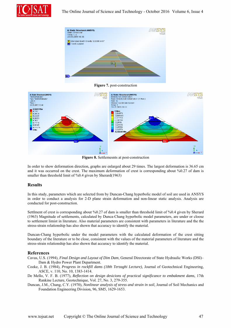
Figure 7. post-construction

Figure 8. Settlemesnts at post-construction

In order to show deformation direction, graphs are enlarged about 29 times. The largest deformation is 36.65 cm and it was occurred on the crest. The maximum deformation of crest is corresponding about %0.27 of dam is smaller than threshold limit of %0.4 given by Sherard(1963) Results In this study, parameters which are selected from by Duncan-Chang hyperbolic model of soil are used in ANSYS in order to conduct a analysis for 2-D plane strain deformation and non-linear static analysis. Analysis are conducted for post-construction. Settlment of crest is corresponding about %0.27 of dam is smaller than threshold limit of %0.4 given by Sherard (1963) Magnitude of settlements, calculated by Dunca-Chang hyperbolic model parameters, are under or cloose to settlement limist in literature. Also material parameters are consistent with parameters in literature and the the stress-strain relationship has also shown that accuracy to identify the material. Duncan-Chang hyperbolic under the model parameters with the calculated deformation of the crest sitting boundary of the literature or to be close, consistent with the values of the material parameters of literature and the stress-strain relationship has also shown that accuracy to identify the material. References Cavus, U.S. (1994), Final Design and Layout of Dim Dam, General Directorate of State Hydraulic Works (DSI)–

Dam & Hydro Power Plant Department. Cooke, J. B. (1984), Progress in rockfill dams (18th Terzaghi Lecture), Journal of Geotechnical Engineering,

ASCE, v. 110, No. 10, 1383-1414. De Mello, V. F. B. (1977), Reflection on design desicions of practical significance to embakment dams, 17th

Rankine Lecture, Geotechnique, Vol. 27, No. 3, 279-355. Duncan, J.M., Chang, C.Y. (1970), Nonlinear analysis of stress and strain in soil, Journal of Soil Mechanics and

Foundation Engineering Division, 96, SM5, 1629-1653.



Duncan, J.M., Byrne, P., Wong, K.S. and Babry, P. (1980), Strength, stress-strain and bulk modulus parameters for finite element analyses of stresses and movements in soil masses, in Report No: UCB/GT/80–01, University of California at Berkeley.

Fumagalli, E. (1969), Test on cohesionless materials for rockfill dams, Journal of Soil Mechanics and Foundation Engineering Division, ASCE, 95, SM1, 313-332.

Janbu, N. (1963), Soil compressibility as determined by oedometer and triaxial tests, Proceedings, European Conference on Soil Mechanics and. FoundationEngineering, Wiesbaden, West Germany, Vol. 1, pp. 19-25.

Khalid, S., Singh, B., Nayak, G.C., and Jain, O.P. (1990), Nonlinear analysis of concrete face rockfill dam, Journal of Geotechnical Engineering, ASCE, Vol.116, No.5, pp.822-837

Kocbay, A. (2010), Concrete faced rockfill dams example: Dim Dam (Antalya-Turkey), Conference Paper, ISRM International Symposium - 6th Asian Rock Mechanics Symposium, 23-27 October, New Delhi, India.

Kondner, R. (1963), Hyperbolic Stress-Straim Response of Cohesive Soils, Journal of Soil Mechanics and Foundation Engineering Division, ASCE, Vol.89, SM1, 115-143.

Leps, T. M. (1970), Review of shearing strength of rockfill, Journal of Soil Mechanics and Foundation Engineering Division, ASCE, 96, SM4, 1159-1170.

Marachi, N. D., Chan, C. K. and Seed, H. B. (1972), Evaluations of properties of rockfill materials, Journal of Soil Mechanics and Foundation Engineering Division, ASCE, 98, SM1, 95-114.

Marsal, R. J. (1967), Large scale testing of rockfill materials, Journal of Soil Mechanics and Foundation Engineering Division, ASCE, 93, SM2, 27-43.

Saboya, F. Jr. and Byrne, P.M. (1993), Parameters for stress and deformation analysis of rockfill dams, Canadian Geotechnical Journal, 30, 690–701.

Sherard, J. L., Woodward, R. J., Gizienski, S. F., and Clevenges, W. A. (1963), Earth and Earth-Rock Dams, John Wiley & Sons, New York.



TIME-DEPENDENT CHANGE OF SEISMIC VELOCITIES ON LOW-STRENGTH CONCRETE

Nevbahar SABBAĞ1, Osman UYANIK1

1 Suleyman Demirel University, Faculty of Eng., Depart. of Geophysical Eng. Isparta/TURKEY

[email protected]

Abstract: In this study, time-dependent change of Seismic velocities on low-strength concrete samples was investigated. For this purpose, 150x150x150 mm sizes 9 cubic samples were prepared for each of 4 different concrete designs. Water cure was applied on prepared samples. Seismic Ultrasonic P and S waves travel time measurements were made on the two opposed surfaces of the samples for 90 days during specific time periods and P and S wave velocities were calculated. Time dependent curves of Seismic velocity values that obtained from performed these studies depending on the time were formed. While Seismic velocities of saturated samples increased depending on the time, thought to be after 72nd day very few decline in Seismic velocities were observed. Reasons of this decrease in Seismic velocity values, bring thought of samples remain more water than required and the long-term exposed to water adversely affect characteristics of concrete samples. *This study was supported with OYP05277-DR-14 Project No. by SDU Project No.Keywords: Concrete, Cubic sample, P wave, S wave, Water cure, Time

INTRODUCTION

Concrete strength is determined with coring and subjected this core to the compressive strength test destructively. To determine the time-dependent change of the same sample is not possible with the conventional method as compressive strength test. But alternatively determining the time-dependent change of the concrete strength is possible non-destructively by Seismic velocities. At the result of several studies concrete strength can be determined from the Seismic pressure wave (P) velocity. However, the P wave velocity is affected with water or gas saturated voids or fractures of the concrete. So, it is clear that a third parameter is needed which unaffected from the water or gas saturation and controller of the relationship between P wave velocity and concrete strength dispersion. This parameter may be shear (S) wave velocity which depends on several features such as concrete strength, aggregate type and cement properties. Also by using of pressure and shear wave velocities together can be interpreted pores of the concrete to dry or water saturated. We can identify cracks, voids and decomposition situation in the concrete with Seismic Ultrasonic method. After determining P and S wave velocities of the concrete the dynamic elastic properties of concrete (shear modulus, Poisson ratio, modulus of elasticity, bulk modulus) can be determined from the elasticity theory (Bahadır, 1984; Swamy, 1984; Keiller, 1985; Jenkins, 1985; Akça, 1991; Uyanık, 1991, Uyanık et al., 2013).

Before prepared cubic concrete samples of being subjected to Uniaxial Compressive Strength test, the effect of time-dependent change of the pressure (P) and shear (S) wave measurements have been tried to be observed by the Seismic Ultrasonic method. In the literature, time-dependent change of concrete samples was evaluated from different points of view. Relationship between concrete strength and aggregate gradation, different water/cement rates, cement type, moisture and temperature, effect of shrinkage and creep events were tried to be observed time-dependently on concrete samples (Istanbulluoğlu, 1988; Cheng et al., 2004; Kerr, 2007; Phan and Carino, 2001; Keleştemur and Star, 2005; Vittorio, 2011; Soykan and Özel, 2014). However, determining the time-dependent change of Seismic Ultrasonic P and S wave measurements were not done before. Performed study constitutes a first in this regard. Scope of the study three different concrete designs indicates low strength approximately 5, 10 and 15 MPa were compared to one prepared concrete design with normal strength approximately 30 MPa (Taşdemir et al., 2004). Thus, the effect of Seismic velocities on low-strength concrete could be put forward more clearly.

ULTRASONIC SEISMIC METHOD

Non-destructive Ultrasonic Seismic method can be used for determine the mechanical properties of concrete in-situ and in laboratory. In this method, Seismic P wave known as sound wave, as well as Seismic S wave measurements are made. P-waves, also known as primary, longitudinal, pressure or sound wave, move compress and dilates to the particles. These waves can be spread in the solid, liquid and gas environment. But S waves can only spread in environments that resistant to the change of shape. As is known, S waves are not propagation in



these liquid and gas environments due to absence of resistant against the change of shape. This wave velocity values depend on the rigidity and density of their spreading body (Uyanık, 1991; Öztürk, 1993; Pampal, 2000). Zero setting of the device should be performed before starting of the P and S wave measurement by ultrasonic equipment. Zero setting is process of receive the electric pulse and convert to a Seismic pulse by transducer. This process takes a few micro-seconds and this delay should be removed. However, the zero setting must be carried out separately for P and S waves.

Fig. 1 Seismic Ultrasonic P and S wave measurement equipment and taking measures

After zero setting is finished, the required settings from the P or S wave options are made. So, it is possible to pass the P or S wave travel time measurements. Ultrasonic energy has been delayed by an air gap. Therefore, to provide a very good transmission is necessary between the sample and the receiver-transmitter probe. In order to ensure fully transmission must be used improver transmission substance grease oil, etc. However, such materials should not be used in the S-wave travel time measurement. Smooth and even surface of the samples is one of the most important factors affecting the measurement. Transmitter and receiver probes are available in Seismic Ultrasonic devices. The arrival time is recorded one side by sending a wave the other side of the sample (Figure 1). The velocity (V) is determined from ratio of the distance (length) between the transmitter and receiver probes (L) to the arrival time (t) (Uyanık, 1991; IAEA, 2002; Sabbağ et. al., 2014).

(1)

Ultrasonic Seismic P and S wave measurements can be done on samples in laboratory or in-situ. By this method measurement can be determined cracks, void and alteration situation of the concrete, as well as to the mechanical properties of concrete (Figure 2). One of the most important features of the method is to achieve results quickly without any damage to the structure. However, it is important for the interpretation of the concrete quality that to determine whether it is received on the reinforcement in-situ measurement. After the determination P and S wave velocities of concrete, elastic properties of the concrete (modulus of elasticity, shear modulus, bulk modulus, Poisson ratio) are determined from the elasticity theory (Uyanık, 2012).



Fig. 2 Ultrasonic Seismic P and S waves travel time records (Uyanık et. al., 2015b) Voids in the concrete are the most important factor of affecting the Seismic velocities. As is known, passing of the Seismic P waves in the porous material of the concrete are slow. Therefore, height of the Seismic velocity indicating that the concrete quality is high, low of the Seismic velocity indicating that the quality is low. Also, because of S waves are not spread in the voids and the available liquid in the voids provide to us having a review about the concrete is stringent or loose (Leslie and Cheesman, 1950; Whitehurst, 1951; Uyanık, 2012). UNIAXIAL COMPRESSIVE STRENGTH TEST Most commonly used of non-destructive method is receiving of cylindrical samples (cores) from the concrete of the structure and subjected to breakage effect under the axial force. This method gives concrete strength in structure/in-situ with highest reliance despite of drawbacks such as cost, speed and its ruin in the structure (Arıoğlu and Arıoğlu, 1998; Erdoğan, 2003, Başka, 2006; Uyanık et. al., 2015a). Unless otherwise indicated Compressive strength is determined at 28 days samples. Uniaxial compressive strength of the concrete sample is described as its resistance of against breakage. According to the standard of related to sample sizes length/diameter ratio of cylindrical samples should be 2- 2.5 in the test. Generally for this 150x300mm size cylindrical or 150x150x150mm dimensional cubes are used. Because of the size effect, visible strengths of material vary for different sizes examples. Small of the sample size is relatively increases strength and leads to increasing volatility in the results.

Fig. 3 Applying Uniaxial Compressive Strength Test on samples (Sabbag and Uyanık, 2015) The prepared samples are placed between the steel plates of the hydraulic press. If load of applying at the time of sample breakage is called P and the surface area of the sample is called A, Uniaxial Compressive Strength is found as P/A (Figure 3). The water content of the sample can significantly influence the compressive strength test results during the test. After preparation, samples must be kept under normal atmospheric conditions at room temperature



until testing is performed. In order to make the compressive strength test, samples are dried in an oven at 105 ± 5 °C until the weights unchanged. Different water content ratio of the sample may be required to be tested. Compressive strength varies with coming stress of perpendicular or parallel direction to the discontinuities and layer surface. Strength in perpendicular direction to the discontinuity surface is greater than the strength of obtained in parallel (Köse and Kahraman, 1998). The compressive strength of concrete is affected by changes of loading speed. While the applied speed of application stress to the concrete sample decreases (load is applied upon a longer period) the sample is broken under a smaller stress. In other words, the pressure obtaining in the low-load speed of the sample strength is lower. This case occurs with the amount of creep due to the load stay longer on the sample. On the other hand, the high loading rate applied on samples is broken under a big load, that is, higher compressive strength value is obtained (Erdoğan, 2003; Felekoğlu and Türkel, 2004). THE EFFECT OF WATER CONTENT The water content of the concrete (w) is expressed as the ratio of the water mass in the concrete to the mass of solid particles. The amount of water contained in unit volume of material can be expressed by mass or volume. Concrete strength decreases with increasing water/cement ratio (Mertol, 2010). Also the water must fill the spaces between particles except from the particle surfaces absorption. The excess water provides fluidity as separating of the particle by a water layer. Increasing the amount of water will increase fluidity and will provide that concrete to be compressed easily. Indeed, the total water content is the most important parameter that provides the main binding. However, the excess water is reduced the binding and causes decomposition and desorption. There are two types of voids in cement paste. One of these is small void between the gel particles; the other is large capillary void between gel particles and aggregates. In order to the hydration of cement using redundant water remains in the space of mass concrete and can significantly affect the durability of concrete. The excess water is lost along with the drying of the concrete and reduces the resistance when causing an increase in the porosity of the concrete. Interconnected voids which create channels to pass of harmful substances from outside and thus interconnected spaces increase the permeability of concrete. Because of the void ratio and therefore permeability of concrete are very high, unable to protect the reinforcement (Bayazıt and Yalçın, 1970). DATA PROCESSING Concrete is a composite building material which obtained as a result of gaining strength harden over time of different sizes aggregates such as sand, gravel, granular mineral materials (gravel etc.) mixing with water and cement paste. In this study the type of aggregate was used as crushed stone aggregate. The rocks broken and crushed desired sizes of form which taken from the quarry of near Antalya Boyali pond by stone crusher, so that the aggregate was formed by using materials such as crystallized limestone, marble etc. taken from rock stockyard, per unit volume mass, specific weight, mass of water absorption, volume of water absorption, pressure loss after freeze, determination of the frost strength with sodium sulfate, Los Angeles abrasion (100 rpm/500 rpm) laboratory tests were carried out. 25% coarse aggregate, 23% medium gravel, 52% sand prepared using aggregate grain size of the largest aggregate Dmax = 63 mm. A kind of cement as CEM II/B-LL composite Portland cement (limestone (total organic carbon): 0.2%) were used for preparation of the designs. As chemical additives Aermix was used for air-entraining admixture and Fluico was used for super plasticizer concrete admixture. The mixtures were prepared by using of the potable water supply. Slump (crash) test value was taken as 12 for all mixtures. This study was conducted with the different mixing ratio of concrete. Accordingly, showing different concrete strength four designs 150x150x150mm size cubic samples were prepared. 9 cubic samples were available for each design. Scope of study three different concrete designs indicates low strength approximately 5, 10 and 15 MPa were compared to one prepared concrete design with normal strength approximately 30 MPa (Taşdemir et al., 2004). Thus the effect of Seismic Velocities on low strength concrete could be more clearly.



Fig. 4 Drying in an oven and applying water cure of the samples for the determination of water content

In order to preparation of the cubic samples, different proportions of water, cement, aggregates and additives were used with approximately 5 MPa, 10 MPa and 15 MPa three low-strength concrete designs and with approximately 30 MPa normal strength concrete design. After the determination of the weight and density Ultrasonic seismic P and S wave measurements were taken from two opposing surfaces of the samples for determine the water content of the samples 3rd, 7th, 28th, 41st, 56th, 65th, 72nd and 90th days. Then it dried in an oven at 105oC for 24 hour. Then removed dry form weight measurements of samples made enacted, Seismic Ultrasonic measurements were taken. The data were grouped for monitoring velocity changes depending on the time. Until specified time period of the measurement day samples are waited in the curing pool (Figure 4). 3 samples of each design were broken 7th, 28th and 90th days by Uniaxial Compressive Strength Test and averages of values were obtained. EVALUATIONS The studies carried out on 4 different concrete designs that the first arrival times of P and S records were determined by Seismic Ultrasonic device before samples being subjected to uniaxial compressive test. Seismic velocities were obtained by using size and the first arrival time of these samples. Measurements have repeated at predetermined time intervals in order to observe the time-dependent change of these velocities. In this context, it is possible to observe the change of the samples in Figure 5.

Fig. 5 Time-dependent change of Seismic P wave Velocity (a) Seismic S wave Velocity (b) and Seismic Velocities ratio (c) for 4 designs



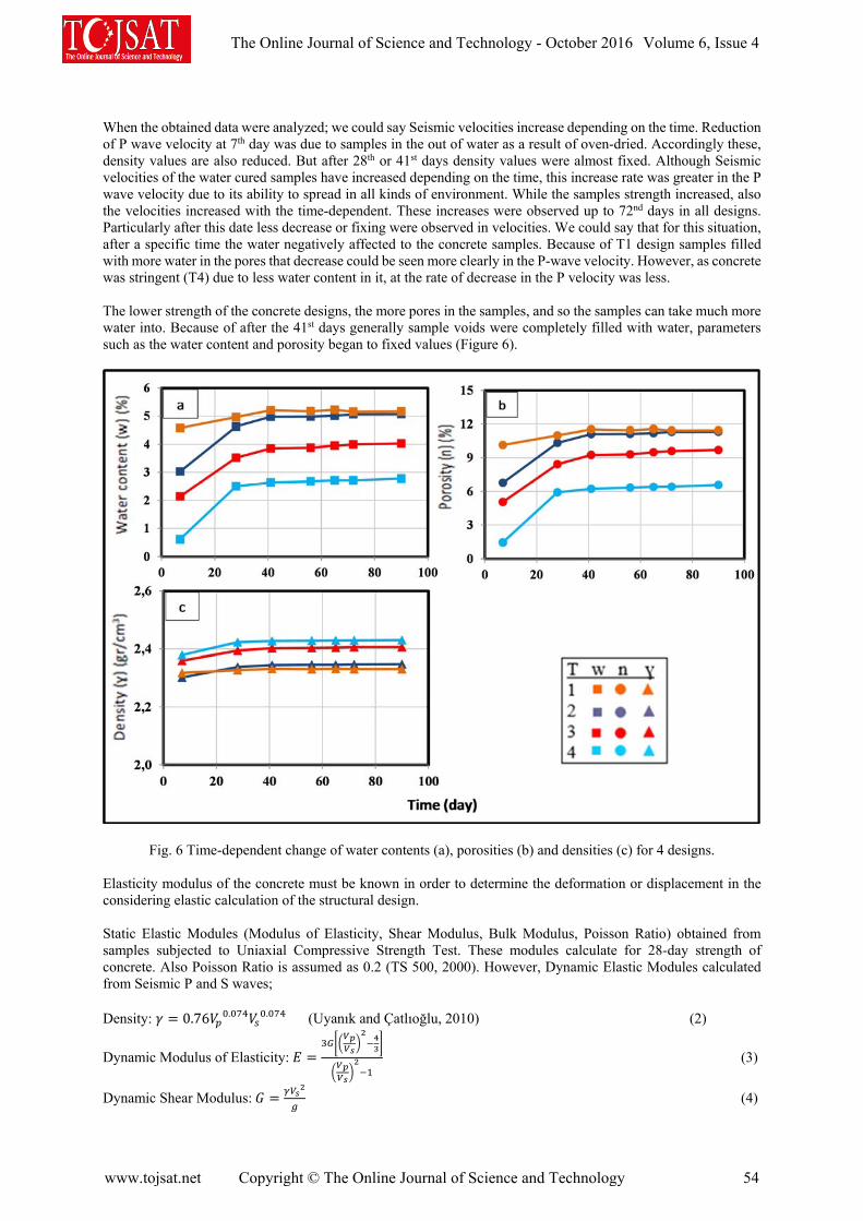
When the obtained data were analyzed; we could say Seismic velocities increase depending on the time. Reduction of P wave velocity at 7th day was due to samples in the out of water as a result of oven-dried. Accordingly these, density values are also reduced. But after 28th or 41st days density values were almost fixed. Although Seismic velocities of the water cured samples have increased depending on the time, this increase rate was greater in the P wave velocity due to its ability to spread in all kinds of environment. While the samples strength increased, also the velocities increased with the time-dependent. These increases were observed up to 72nd days in all designs. Particularly after this date less decrease or fixing were observed in velocities. We could say that for this situation, after a specific time the water negatively affected to the concrete samples. Because of T1 design samples filled with more water in the pores that decrease could be seen more clearly in the P-wave velocity. However, as concrete was stringent (T4) due to less water content in it, at the rate of decrease in the P velocity was less. The lower strength of the concrete designs, the more pores in the samples, and so the samples can take much more water into. Because of after the 41st days generally sample voids were completely filled with water, parameters such as the water content and porosity began to fixed values (Figure 6).

Fig. 6 Time-dependent change of water contents (a), porosities (b) and densities (c) for 4 designs. Elasticity modulus of the concrete must be known in order to determine the deformation or displacement in the considering elastic calculation of the structural design. Static Elastic Modules (Modulus of Elasticity, Shear Modulus, Bulk Modulus, Poisson Ratio) obtained from samples subjected to Uniaxial Compressive Strength Test. These modules calculate for 28-day strength of concrete. Also Poisson Ratio is assumed as 0.2 (TS 500, 2000). However, Dynamic Elastic Modules calculated from Seismic P and S waves; Density: 0.76 . . (Uyanık and Çatlıoğlu, 2010) (2)

Dynamic Modulus of Elasticity: (3)

Dynamic Shear Modulus: (4)



Dynamic Bulk Modulus: (5)

Poisson Ratio:μ (6)

Dynamic modulus of elasticity is equal to changing of a very small deformation. Usually this is greater than static modulus of elasticity from 20% to 40% by Sonic Resonant frequency method. The initial static modulus of elasticity is approximately equal to dynamic modulus of elasticity. Using the dynamic modulus is suitable for Seismic and blast loadings of structures (Mc Cormac and Nelson, 2005). While Static Elastic Modules calculated from Uniaxial Compressive Strength test destructively, Dynamic Elastic Modules calculated from Seismic P and S wave velocities non-destructively. Dynamic Elastic modules calculate for the same concrete samples every time. For this purpose, these modules could be calculated up to 90 days. As well as the P-wave velocity also obtaining of S-wave velocity enables to reach dynamic elastic parameters (Figure 7).

Fig. 7 Time-dependent change of (a) Dynamic Elasticity Modulus (b) Dynamic Shear modulus (c) Dynamic Bulk Modulus and (d) Poisson Ratio for 4 designs.

CONCLUSIONS Seismic velocities of same water-saturated concrete increase depend on time. P and S wave velocities of water-saturated concrete designe under 50MPa change between 2.8-4.6km/s and 1.6-2.5 km/s, respectively. Densities increases depend on concrete strength time dependently. After saturation (41st days) water content and porosity are fixed depend on time. Dynamic modules are increases with increasing of strength time dependently. Dynamic Elasticity modulus (Ed) change between 18-40 GPa, Dynamic Shear modulus change between (Gd) 8-16 GPa, Dynamic Bulk modulus change between 10-37 GPa for low-strength concretes. Poisson Ratio changes



between 0.22-0.35 depend on time. This result show that Poisson ratio not stable as agreed 0.2 value in static elastic module accounts of concrete. Poisson ratio changes with water saturation of concrete. Concrete strength can be calculated from Seismic velocities (P and S wave) non-destructively. Moreover, dynamic elastic modules are also calculated from Seismic velocities easily. Also, this study is a first for determining of dynamic elasticity modules by Ultrasonic Seismic method and time dependent change of these modules. Dynamic modules of water-saturated concrete take different values depend on time. REFERENCES Akça, A. (1991). Investigation Factors of the Affecting Core Strength That Used to Determine Concrete Strength,

Master Thesis, KTU. Science and Technology Institute, Trabzon. Arıoğlu, E. and Arıoğlu, N. (1998). Concrete Core Test and Evaluation of The Upper and Lower Structure, Evrim

Publisher. Istanbul. Bahadır, M. (1984). Detection of Concrete Strength by Aid of Core, Master Thesis, KTU, Institute of Science and

Technology, Trabzon. Cheng, F.P., Kodur, V.K.R. and Wang, T.C. (2004). Stress-Strain Curves for High Strength Concrete at Elevated

Temperatures, Journal of Materials in Civil Engineering, V.16, No.1, pp. 84-90. Erdoğan, T. (2003). Concrete, METU edition. Felekoğlu, B. and Türkel, S. (2004). Use of overdose plasticizer effect on Fresh and Hardened Concrete

Admixtures. Dokuz Eylul University, Faculty of Engineering and Science Engineering Journal, 6, 1, 77-89. IAEA (International Atomic Energy Agency). (2002). Guidebook on non-destructive testing of concrete structures,

Training Course Series No. 17, VIENNA. Istanbulluoğlu, S. (1988). Factors Affecting The Concrete Compressive Strength And A Study On Selection Of

Ramble Concrete, Mining Journal, 27(3). Jenkins R.S. (1985). Non Destructive Testing: An Evaluation Tool, Concrete International: Design and

Construction, Vol. 7, no. 2, Feb., pp. 22-26. Keiller A. P. (1985). Assessing The Strength Of The In Situ Concrete, Concrete International: Design And

Construction, Vol. 7, no. 2, Feb. pp. 15-21. Kerr, E. A. (2007). Damage Mechanisms and Repairability of High Strength Concrete Exposed to Elevated

Temperatures, University of Notre Dame. Köse, H., Kahraman, B. (1999). Rock Mechanic. Dokuz Eylul University press, No: 177. Leslie, J. R., Cheesman, W. J. (1950). An Ultrasonic Method of Studying Deterioration and Cracking In Concrete

Structures, ACI Journal Proceedings, 46, 17-36. McCormac, J.C. and Nelson, J.K. (2005). Design of Reinforced Concrete, 6th Edition. Mertol, H., C. (2010). The Comparison of Normal and High Strength Concrete Used in The Design, 5th National

Congress and Exhibition of Building Materials Presentations. Öztürk, K. (1993). Prospecting Geophysics (Seismic), Istanbul University Faculty of Engineering, Istanbul. Pampal, S. (2000). The Effect of the Earthquake, Earthquakes, alpha / current Bookstores, Ankara Phan, L. T. and Carino, N. J. (2001). Mechanical Properties of High-Strength Concrete at Elevated Temperatures,

NISTIR 6726, Building and Fire Research Laboratory, National Institute of Standards and Technology, Gaithersburg, MD.

Sabbağ, N. and Uyanık, O. (2015). Investigating Effect of Reinforcement on Concrete Strength by Seismic Velocities, Young Geoscientist Congress, 5-7 June, Izmir

Sabbağ N., Ekinci,B., Uyanık O., Öncü Z., Akdemir S., Türker E. (2014). Developing Strength Chart Of Saturated Concrete By Using Seismic P and S-Wave Velocities in Laboratory. AGU Fall Meeting, USA.

Soykan, O. and Özel, C. (2014). Effect of Polymer Physical and Mechanical Properties of Concrete Curing Time, Cumhuriyet University, Journal of Science (CFD), Vol.35, No. 2 (2014), ISSN: 1300-1949.

Swamy R. N. (1984). Aliamah Assessment Of In Situ Concrete Strength By Various Non-Destructive Tests, Non Destructive Testing International, Vol. 17 no.3, pp. 139-146.

TS 500. (2000). Standard of Design and Constructions Rules of Concrete Structure. Uyanık, O. (1991). Rock Mechanics and Geophysics Laboratory Association Importance of Parameters, Dokuz

Eylul University, Faculty of Engineering and Architecture, Geophysical Eng. Department, Izmir. Uyanık, O. and Çatlıoğlu, B. (2010). Determination of Density from Seismic Velocities, The 19th International

Geophysical Congress and Exhibition of Turkey, 23 – 26 November Ankara. Uyanık, O. 2012. Determination of Concrete Strength with Seismic Velocity, Geophy. Bulletin. 23(70): 25-30. Uyanık, O., Şenli, G. and Çatlıoğlu, B. (2013). Building of The Non-Destructive Geophysical Methods

Determination of Concrete Quality, SDU International Journal of Technological Sciences 5 (2): 156-165.



Uyanık, O., Sabbağ, N., Ekinci, B., Öncü, Z. (2015a). The Importance of Using Seismic Ultrasonic Velocities together in Determining of Concrete Strength, ICENS2015, Makedonya.

Uyanık, O., Ekinci, B., Sabbağ, N., Öncü, Z. (2015b). Investigation of Concrete Strength by using P and S Wave Velocities, Young Geoscientist Congress, 5-7 June, Izmir.

Vittorio, S. D. (2011). Time-Dependent Behaviour of Reinforced Concrete Slabs, Alma Mater Studiorum - University of Bologna Faculty of Engineering, International Master Course in Civil Engineering, DICAM, Civil, Environmental and Materials Engineering, Advanced Design of Structures Thesis.

Whitehurst, E. A. (1951). Soniscope Test Concrete Structures, ACI Journal Proceedings, 47, 443-444.



WAVELENGTH DIVISION MULTIPLEXING AND ENERGY EFFICIENCY

Öznur ŞENGEL

İstanbul Kültür University Computer Engineering

Bakırköy-İstanbul/Turkey [email protected]

Muhammed Ali AYDIN İstanbul University

Computer Engineering Avcılar-İstanbul/Turkey [email protected]

Abstract: Energy is hot topic in the improvements of the technology because energy efficiency topic is very important for future generations with the growing population in the world. Recently, hardware and functional structures in network are provided more data transmission with less energy and improvement the usage of communication tools on the internet. Telecommunications companies lean in to develop their infrastructure with energy efficiency. Hardware and functional routing methods are developed for energy efficiency and quality of service while fiber infrastructure with WDM networks is preferred to provide fast communication. This study gives information about Optical Circuit Switching (OCS), Optical Packet Switching (OPS), Optical Burst Switching (OBS), and Parallel Optical Burst Switching (POBS) in Wavelength Division Multiplexing (WDM) networks and their strategies, methods and studies to improve energy efficiency. Keywords: Energy Efficiency, Wavelength Division Multiplexing (WDM), Optical Circuit Switching (OCS), Optical Packet Switching (OPS), Optical Burst Switching (OBS), Parallel Optical Burst Switching (POBS)

Introduction Nowadays, communication on the internet are increasing, the economic and environmental impact of this situation has been discussed. According to a survey in United States, 1-7% of the electricity is consumed by internet tools (Tucker, 2009) and this rate increase about 50% in each year (Plepys, 2002). The usage of the internet is increasing 40% day by day in North America (Kilper, 2011). Increment of communication over the internet is seemed small scale now, but it is expected to reach significant number in the near future. As long as this increment is continued, energy consumption will be increase evenly. The increment of the usage of internet means not only increment on network users but also increment of the bandwidth for each user (Tucker, 2012). Researchers start to improve more energy efficient system to balance energy consumption on the usage of internet. Also, they study with energy network technologies. Nowadays, qualified and full time communication is very important. The means of more quickly communication is faster computer components and more energy consumption. The existing network infrastructure such as servers, amplifiers, routers, filters, storage devices and communication links must strengthen to ensure fast and quality communication. Although reinforcement of the network infrastructures provides desired bandwidth, it consumes more energy. This situation makes energy efficiency topic more popular among researchers. Energy consumption originated from internet is increased day by day in developed and developing nations (Hinton, 2011). Society in economic growth is concerned to improve communication units with the same rate of increment on communication. This recovery means that function of the communication tools must improve and at the same time more energy is consumed for each developing units. As long as communication over internet is increasing, power consumption is increased. Telecom companies make their infrastructures more suitable with new technology to provide fast data transmission. First choice of the telecom companies is optical network that provides faster data transmission. Network capacity can be increased with different wavelengths instead of placing more fiber lines. Therefore, wavelength division multiplexing are the most popular systems for telecom companies.



Energy is conserved 45% in wavelength division multiplexing (Shen, 2009). It can be possible with using wavelength grooming mechanism to transmit lightpaths in optical domain. It equals to save about 500 million dollars in a year for middle networks. WAVELENGTH DIVISION MULTIPLEXING (WDM) Wavelength Division Multiplexing is composed more than one different wavelength in a fiber. Each wavelength is accepted one channel. WDM includes multiplexer that gather signals, demultiplexer that separate signals and amplifiers. Each light source has different wavelength output in WDM network. Optical signals, which come from different wavelength transmitters, are multiplexed to transmit one fiber by wavelength multiplexer (see Figure 1). On the other hand, wavelength multiplexed lights from fiber is separated to different wavelength by demultiplexer and each wavelength transmit to receiver. During the transmission, amplifier can be used to strengthen signals before demultiplexer and after multiplexer.

Figure 1. Wavelength Division Multiplexing (WDM)

Wavelength number on a fiber is increased with WDM network and it is the cheapest way for data transmission. Increasing fiber number is more expensive than increasing channel number in fiber (Aydın, 2009). So, WDM network is become popular among telecom companies and was established telecommunications backbone network. Telecom companies try to find cheaper solution inadequacy existing infrastructure to rapid development of the internet and incremental bandwidth requirements. Fast transmission with Wavelength Division Multiplexing communication systems is provided by using fiber infrastructure, improving network capacity is provided by wavelength with using little fiber cable. Although working on WDM is complicate and expensive at the first time, to develop WDM network has become cheaper with the understanding of the dynamic structure of WDM. Bandwidth requirements in optical network have been solved with OCS (Optical Circuit Switching), OPS (Optical Packet Switching), and OBS (Optical Burst Switching). OPTICAL CIRCUIT SWITCHING (OCS) Lightpaths are built between network nodes in Optical Circuit Switching that is the one of optical network technologies (see Figure 2). There are different wavelengths in each lightpath. Packet in network is transferred in optical form from ingress node to egress node. Wavelengths are reserved to generate a lightpath to transmit packet from one node to another. Reserved path are released after packet is received. Not only same wavelength but also different wavelength is reserved between nodes. This can be with wavelength converter. If the wavelength converter does not exist, same wavelength can reserve.

Figure 2. Lightpath in OCS



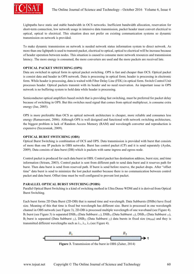
Lightpaths have static and stable bandwidth in OCS networks. Inefficient bandwidth allocation, reservation for short-term connection, low network usage in intensive data transmission, packet header must convert electrical to optical, optical to electrical. This situation does not prefer on existing communication systems so dynamic transmission on network is provided. To make dynamic transmission on network is needed network status information system to direct network. As more than one lightpath is used to transmit packet, electrical to optical, optical to electrical will be increase because of header operation between nodes. This situation is caused to consume more network resources and transmission latency. The more energy is consumed, the more converters are used and the more packets are received late. OPTICAL PACKET SWITCHING (OPS) Data are switched in optical form in optical packet switching. OPS is fast and cheaper than OCS. Optical packet is consist data and header in OPS network. Data is processing in optical form; header is processing in electronic form. While header is processing, data is waited with Fiber Delay Line (FDL) in optical form. Switch Control Unit processes header. Optical packets transmit with its header and no need reservation. An important issue in OPS network is no buffering system to hold data while header is processing. Semiconductor optical amplifiers based switch that is providing fast switching, must be preferred for packet delay because of switching in OPS. But this switches need signal that comes from optical multiplexer, is consume extra energy (Jue, 2005). OPS is more preferable than OCS as optical network architecture is cheaper, more reliable and consumes less energy (Ramaswami, 2006). Although OPS is well designed and functional with network switching architecture, the biggest problem is lack of Random Access Memory (RAM) and wavelength converter and reproduction is expensive (Szczesniak, 2009). OPTICAL BURST SWITCHING (OBS) Optical Burst Switching is combination of OCS and OPS. Data transmission is provided with burst that consists of more than one IP packets in OBS networks. Burst has control packet (CP) and it is send separately (Aydın, 2009). Data consists of data burst (DB) which is packets with same ingress and egress node. Control packet is produced for each data burst in OBS. Control packet has destination address, burst size, and time information (Sriram, 2003). Control packet is sent from different path to send data burst and it reserves path for burst. Then data burst is send from reserved path. If burst is send before reserve, the packet drops. After “offset time” data burst is send to minimize the lost packet number because there is no communication between control packet and data burst. Offset time must be well configured to prevent lost packet. PARALLEL OPTICAL BURST SWITCHING (POBS) Parallel Optical Burst Switching is a kind of switching method in Ultra Dense WDM and it is derived from Optical Burst Switching. Each burst forms 2D Data Burst (2D-DB) that is named time and wavelength. Data Subbursts (DSBs) have fixed size. Meaning of this that time is fixed but wavelength has different size. Burst is processed in one wavelength channel in OBS network (see Figure 3), 2D-DB is processed multiple wavelength of one waveband (see Figure 4). B1 burst (see Figure 3) is separated DSB11 (Data Subburst 11), DSB12 (Data Subburst 12), DSB13 (Data Subburst 13), B2 burst is separated (Data Subburst 21), DSB22 (Data Subburst 22) data bursts in fixed size (mDSB) and they is

transmitted different wavelengths such as 1, 2, 3 (see Figure 4).

Figure 3. Transmission of the burst in OBS (Zaiter, 2014)



Figure 4. Transmission of the burst in POBS (Zaiter, 2014)

Optical Signal in fiber is analyzed B1, B2, ..., BM waveband with Fiber to Band (FTB) burst multiplexer (see Figure 5). B1, B2, ..., BM waveband with Band to Fiber (BTF) burst multiplexer is analyzed to exit fiber. Control

packet is transmitted separately with Control Channel (c). First of all, control packet converts optical to electrical (O\E) and then is processing in Switching Control Unit (SCU). Lastly, it is converts electrical to optical (E\O) to turn optical environment. Wavelengths with same source- destination node uses one port to switch multiple wavelengths are grouped in one waveband and exit from ingress node (Guo, 2009, Huang, 2007).

Figure 5. Architecture of a POBS core node (Zaiter, 2014)

ENERGY EFFICIENCY IN WAVELENGTH DIVISION MULTIPLEXING To find which equipment on network infrastructures cause more energy consumption is important to manage energy consumption over internet (Hinton, 2011). It depends on changing all old tools of network operator over internet. Aim of the all researches is to get more network performance with low energy. Researchers try to get result from simulation of the new network models, network architecture and protocols that is analyzed and constructed in different network technology. Internet that is using in resident is more than internet that is using in public access such as subway. Also power consumption on internet differs according to building structure. According to Kazovsky (2013) research, power consumption on office and resident in United States of America differs from each other. Energy in office buildings is consumed about 45% on Network Interface Card as increasing of the user number. Energy consumption in resident is changed according to connection type and Wireline LAN interface (Ethernet) is consumed the most energy as we see Figure 6. To construct optical network with high bit rate and use protocols in Passive Optical Network is specified as solutions to provide energy efficiency (Kazovsky, 2013).



Figure 6. Power consumption distribution for current residential networks (Kazovsky, 2013)

The advantages of optical network transmission provide more efficiency (Bathula, 2009a). Energy consumption increases along with increasing transmission data so well constructed network architecture and well routing algorithm in optical network must be specified (Bathula, 2009a). Some researcher specify that optical packet switching (Yoo, 2006) and optical burst switching (Qiao,1999) network are get better solution to electronic routing. Qualified router is consumed approximately10 nj for each bit of data (Baliga, 2009). Optical packet and burst switching need to consume 1 nj for each bit (Tucker, 2006). Furthermore, size of the IP packet affect energy consumption in router. If the IP packet is transmitted with small size, energy will be consumed further. Therefore, router must optimize IP packet size when the IP packet routing schema is transmitted from router to provide energy efficiency (Zhang, 2010). The most energy is consumed on header processing and the transmission of the header. Therefore, burst switching technique that has little header processing is the best alternative. According to Peng (2010), edge switching number must be four times than core switching number, so that burst switching will consume less energy than packet switching. Although, edge burst switches is consumed 20% more energy than edge packet switch, burst switching network is improvable with its other advantages on energy efficiency (Peng, 2010). Energy consumption in optical network calculates summation of power consumption of signal, power consumption of main router and power consumption in amplifiers. Laser resources number that is used and the situation (active or inactive) of optical amplifiers are necessary to reduce power consumption (Bade, 2015). Moreover, to set sleepy mode part of the modem/ONU reduces power consumption significantly (Baliga, 2009). Optical Network Unit (ONU) and Optical Line Terminal (OLT) in Passive Optical Network (PON) always must be active so there are different approaches for sleep mode. According to Turna (2015), data transmission is done over one of two OLT cards until data traffic reduces while the other is stay in deep sleep mode. There are more routing algorithms to develop Quality of Services (QoS) while energy efficiency is improved in optical network. According to Bathula (2009a), new routing algorithm that is specified some node as sleep with threshold and is checked suitable of wavelength is developed. When this methods is compared with shortest path algorithm, this method is given good result both packet delay and energy efficiency. A waveband consists different wavelength with POBS network to improve energy efficiency in OBS network. OBS is consume 15% more energy than parallel optical burst switching with the same scenario (Zaiter, 2014). Energy consumption can be minimized when the value of Burstification Time (BT) and waveband size (Waveband Granularity) is high. According to Zaiter’s (2014) simulation, the network must be configured with high value of Burstification Time and Waveband Granularity in POBS network to reduce energy consumption and drop packet number.



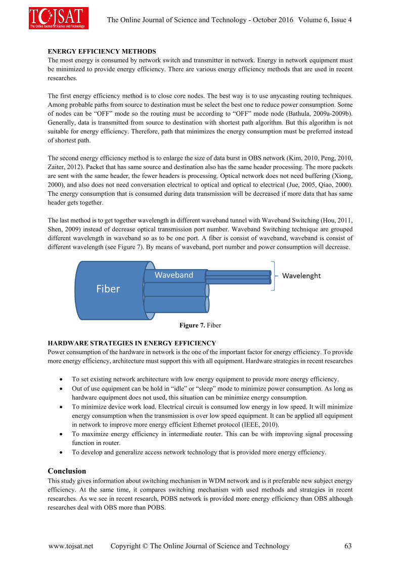
ENERGY EFFICIENCY METHODS The most energy is consumed by network switch and transmitter in network. Energy in network equipment must be minimized to provide energy efficiency. There are various energy efficiency methods that are used in recent researches. The first energy efficiency method is to close core nodes. The best way is to use anycasting routing techniques. Among probable paths from source to destination must be select the best one to reduce power consumption. Some of nodes can be “OFF” mode so the routing must be according to “OFF” mode node (Bathula, 2009a-2009b). Generally, data is transmitted from source to destination with shortest path algorithm. But this algorithm is not suitable for energy efficiency. Therefore, path that minimizes the energy consumption must be preferred instead of shortest path. The second energy efficiency method is to enlarge the size of data burst in OBS network (Kim, 2010, Peng, 2010, Zaiter, 2012). Packet that has same source and destination also has the same header processing. The more packets are sent with the same header, the fewer headers is processing. Optical network does not need buffering (Xiong, 2000), and also does not need conversation electrical to optical and optical to electrical (Jue, 2005, Qiao, 2000). The energy consumption that is consumed during data transmission will be decreased if more data that has same header gets together. The last method is to get together wavelength in different waveband tunnel with Waveband Switching (Hou, 2011, Shen, 2009) instead of decrease optical transmission port number. Waveband Switching technique are grouped different wavelength in waveband so as to be one port. A fiber is consist of waveband, waveband is consist of different wavelength (see Figure 7). By means of waveband, port number and power consumption will decrease.

Figure 7. Fiber

HARDWARE STRATEGIES IN ENERGY EFFICIENCY Power consumption of the hardware in network is the one of the important factor for energy efficiency. To provide more energy efficiency, architecture must support this with all equipment. Hardware strategies in recent researches

To set existing network architecture with low energy equipment to provide more energy efficiency.

Out of use equipment can be hold in “idle” or “sleep” mode to minimize power consumption. As long as hardware equipment does not used, this situation can be minimize energy consumption.

To minimize device work load. Electrical circuit is consumed low energy in low speed. It will minimize energy consumption when the transmission is over low speed equipment. It can be applied all equipment in network to improve more energy efficient Ethernet protocol (IEEE, 2010).

To maximize energy efficiency in intermediate router. This can be with improving signal processing function in router.

To develop and generalize access network technology that is provided more energy efficiency.

Conclusion This study gives information about switching mechanism in WDM network and is it preferable new subject energy efficiency. At the same time, it compares switching mechanism with used methods and strategies in recent researches. As we see in recent research, POBS network is provided more energy efficiency than OBS although researches deal with OBS more than POBS.



Quality of services such as loss packet, latency and usability come into question while aiming to minimize power consumption. Hybrid structure can be improved in POBS network with less packet delay, buffer memory methods and construct infrastructure to improve energy efficiency in the future.

References Aydın, M.A. (2009). Optik Çoğuşma Anahtarlamalı Sistemlerin Analizi. Doctoral Thesis, İ.Ü. Institute of Science. Bade, M.G., Toycan, M., Walker, S.D. (2015). Cost and energy efficient operation of converged, reconfigurable

optical wireless networks. Optical Switching and Networking. Vol.18, Pages 71-80. Baliga, J., Ayre, R., Hinton, K., Sorin, W. V. & Tucker, R. S. (2009). OSA, Energy Consumption in Optical IP

Networks. Journal Of Lightwave Technology. Vol. 27, No. 13, July 1. Bathula, B.G. & Elmirghani, J.M. (2009a). Energy efficient Optical Burst Switched (OBS) Networks. Proceeding

of the IEEE GLOBECOM Workshops, pp: 1-6. Bathula, B.G. & Elmirghani, J.M. (2009b). Green networks: Energy efficient design for optical networks.

Proceeding of the IFIP International Conference on Wireless and Optical Communications Networks (WOCN'09).

Guo, L., X. Wang, W. Ji, W. Hou & T. Yang. (2009). A new waveband switching method for reducing the number of ports in wavelength-divisionmultiplexing optical networks. Opt. Fiber Technol., 15(1): 5-9.

Hinton, K., Baliga, J., Feng, M., Ayre, R. & Tucker, R. S. (2011). Power Consumption and Energy Efficiency in the Internet. IEEE Network. March/April.

Hou, W., L. Guo & X. Wei. (2011). Robust and integrated grooming for power-and port-cost-efficient design in IP over WDM networks. J. Lightwave Technol., 29(20): 3035-3047.

Huang, Y., Heritage, J.P. & Mukherjee, B. (2007). A new node architecture employing wavebandselective switching for optical burst-switched networks. IEEE Commun. Lett., 11(9): 756-758.

IEEE 802.3az-(2010). Energy Efficient Ethernet. http://www.ieee802. org/3/az/index.html. Jue, J.P. & Vokkarane, V.M. (2005). Optical Burst Switched Networks. Springer, Optical Networks Series. United

States of America, 0-387-23756-9. Kazovsky, L. G., Ayhan, T., Gowda, A., Albeyoglu, K. M., Yang, H. & Ng’Oma, A. (2013). How to Design an

Energy Efficient Fiber-Wireless Network. OFC/NFOEC Technical Digest. Kilper D. (2011). Energy Efficient Networks. OFC. Kim, Y., Lee , C. & Rhee, J.K.K. (2010). Analysis of energy consumption in packet burst switching networks.

Proceeding of the 9th International Conference on Optical Internet (COIN), pp: 1-3. Peng, S., Hinton, K.J., Baliga, J., Tucker, R.S., Li, Z. & Xu, A. (2010). Burst switching for energy efficiency in

optical networks. Proceeding of the 2010 Conference on (OFC/NFOEC) Optical Fiber Communication (OFC), Collocated National Fiber Optic Engineers Conference, pp: 1-3.

Plepys A. (2002). The grey side of ICT. Journal of Environmental Impact Assessment Review, vol. 22, no. 5, pp. 509–523.

Qiao, C. & Yoo, M. (1999). Optical burst switching (OBS)—A new paradigm for an optical Internet. J. High Speed Netw., vol. 8, pp. 69–84.

Qiao, C. & Yoo, M. (2000). Choices, features and issues in optical burst switching. Opt. Netw. Mag., 1(2): 36-44. Ramaswami, R. (2006). Optical networking technologies: what worked and what didn’t. IEEE Communications

Magazine, vol. 44, 9, pp. 132-139, September. Shen, G. & R.S. Tucker. (2009). Energy-minimized design for IP over WDM networks. IEEE/OSA J. Opt.

Commun. Netw., 1(1): 176-186. Sriram, K., Griffith, D. W., Lee, S. & Golmie, N. T. (2003). Optical Burst Switching: Benefits and Challenges. Szczesniak, I. (2009). Overview of optical packet switching. Theoretical and Applied Informatics. ISSN 1896–

5334 Vol.21 (2009), no. 3-4, pp. 167–180, November. Tucker R., Ayre, R. & Hinton, K. (2012). Charting a Path to Sustainable and Scalable ICT Networks. GreenTouch

June Open Forum. Tucker, R. S. (2006). The role of optics and electronics in high-capacity routers. J. Lightw. Technol., vol. 24, pp.

4655–4673, Dec.



Tucker, R.S., Parthiban, R., Baliga, J., Hinton, K., Ayre, R.W. & Sorin, W.V. (2009). Evolution of WDM optical IP networks: A cost and energy perspective. J. Lightwave Technol. 27(3): 243-252.

Turna, Ö.C., Aydın, M.A., Atmaca, T. (2015). A Dynamic Energy Efficient Optical Line Terminal Design for Optical Access Network., vol. 522, pp 260-269.

Xiong, Y., Vandenhoute, M. & Cankaya, H.C. (2000). Control architecture in optical burst-switched WDM networks. IEEE J. Sel. Area. Comm., 18(10): 1838-1851.

Yoo, S. J. B. (2006). Optical packet and burst switching technologies for the future photonic Internet. J. Lightw. Technol., vol. 24, pp. 4468–4492, Dec.

Zaiter, M. J., Yussof, S., Abdelouhahab, A., Cheah, C.L. & Saher, A. (2012). On the energy consumption in Optical Burst Switching (OBS) networks. Proceeding of the IEEE Symposium on Computer Applications and Industrial Electronics (ISCAIE, 2012), pp: 233-236.

Zaiter, M. J., Yussof, S., Cheah, C. L., Abdelouhahab, A. & Salih, A. I. (2014). Energy Efficient Parallel Optical Burst Switching (POBS) Networks. Research Journal of Applied Sciences, Engineering and Technology. 8(2): 253-262.

Zhang, Y., Chowdhury, P., Tornatore, M. & Mukherjee, B. (2010). Energy Efficiency in Telecom Optical Networks. IEEE Communications Surveys & Tutorials. Vol. 12, No. 4, Fourth Quarter.



Documents

The Online Journal of Science and Technology · The Online Journal of Science and Technology - October 2016Volume 6, Issue 4 ... 2Technical University of Liberec, Institute for Nanomaterials,